An Introduction to Univariate GARCHModels

Timo TeräsvirtaSchool of Economics and Management

University of AarhusBuilding 1322, DK-8000 Aarhus C

andDepartment of Economic StatisticsStockholm School of EconomicsBox 6501, SE-113 83 Stockholm

SSE/EFI Working Papers in Economics and Finance, No. 646

December 7, 2006

Abstract

This paper contains a survey of univariate models of conditionalheteroskedasticity. The classical ARCH model is mentioned, and var-ious extensions of the standard Generalized ARCH model are high-lighted. This includes the Exponential GARCH model. Stochasticvolatility models remain outside this review.

Keywords: ARCH; conditional heteroskedasticity; GARCH; non-linear GARCH; volatility modelling

JEL Code: C22

Acknowledgements. This research has been supported by JanWallander�s and Tom Hedelius�s Foundation, Grant No. P2005-0033:1.A part of the work for the chapter was done when the author was vis-iting Sonderforschungsbereich 649 at the Humboldt University Berlin.Comments from Changli He, Marcelo Medeiros and Thomas Mikosch(editor) are gratefully acknowledged. Any shortcomings and errorsare the author�s sole responsibility.

1

1 Introduction

Financial economists are concerned with modelling volatility in asset returns.This is important as volatility is considered a measure of risk, and investorswant a premium for investing in risky assets. Banks and other �nancial insti-tutions apply so-called value-at-risk models to assess their risks. Modellingand forecasting volatility or, in other words, the covariance structure of assetreturns, is therefore important.The fact that volatility in returns �uctuates over time has been known for

a long time. Originally, the emphasis was on another aspect of return series:their marginal distributions were found to be leptokurtic. Returns were mod-elled as independent and identically distributed over time. In a classic work,Mandelbrot (1963) and Mandelbrot and Taylor (1967) applied so-called sta-ble Paretian distributions to characterize the distribution of returns. Rachevand Mittnik (2000) contains an informative discussion of stable Paretian dis-tributions and their use in �nance and econometrics.Observations in return series of �nancial assets observed at weekly and

higher frequencies are in fact not independent. While observations in theseseries are uncorrelated or nearly uncorrelated, the series contain higher-order dependence. Models of Autoregressive Conditional Heteroskedastic-ity (ARCH) form the most popular way of parameterizing this dependence.There are several articles in this Handbook devoted to di¤erent aspects ofARCH models. This article provides an overview of di¤erent parameteriza-tions of these models and thus serves as an introduction to autoregressiveconditional heteroskedasticity. The article is organized as follows. Section2 introduces the classic ARCH model. Its generalization, the GeneralizedARCH (GARCH) model is presented in Section 3. This section also de-scribes a number of extensions to the standard GARCH models. Section 4considers the Exponential GARCH model whose structure is rather di¤er-ent from that of the standard GARCH model, and Section 5 discusses waysof comparing EGARCH models with GARCH ones. Suggestions for furtherreading can be found at the end.

2 The ARCH model

The autoregressive conditional heteroskedasticity (ARCH) model is the �rstmodel of conditional heteroskedasticity. According to Engle (2004), the orig-inal idea was to �nd a model that could assess the validity of the conjectureof Friedman (1977) that the unpredictability of in�ation was a primary causeof business cycles. Uncertainty due to this unpredictability would a¤ect the

2

investors�behaviour. Pursuing this idea required a model in which this un-certainty could change over time. Engle (1982) applied his resulting ARCHmodel to parameterizing conditional heteroskedasticity in a wage-price equa-tion for the United Kingdom. Let "t be a random variable that has a meanand a variance conditionally on the information set Ft�1 (the �-�eld gener-ated by "t�j; j � 1): The ARCH model of "t has the following properties.First, Ef"tjFt�1g = 0 and, second, the conditional variance ht = Ef"2t jFt�1gis a nontrivial positive-valued parametric function of Ft�1: The sequence {"tgmay be observed directly, or it may be an error or innovation sequence of aneconometric model. In the latter case,

"t = yt � �t(yt) (1)

where yt is an observable random variable and �t(yt) = EfytjFt�1g; the con-ditional mean of yt given Ft�1: Engle�s (1982) application was of this type.In what follows, the focus will be on parametric forms of ht; and �t(yt) willbe ignored.Engle assumed that "t can be decomposed as follows:

"t = zth1=2t (2)

where {ztg is a sequence of independent, identically distributed (iid) randomvariables with zero mean and unit variance. This implies "tjFt�1 � D(0; ht)where D stands for the distribution (typically assumed to be a normal or aleptokurtic one). The following conditional variance de�nes an ARCH modelof order q:

ht = �0 +

qXj=1

�j"2t�j (3)

where �0 > 0; �j � 0; j = 1; :::; q� 1; and �q > 0: The parameter restrictionsin (3) form a necessary and su¢ cient condition for positivity of the condi-tional variance. Suppose the unconditional variance E"2t = �2 < 1. Thede�nition of "t through the decomposition (2) involving zt then guaranteesthe white noise property of the sequence {"tg; since {ztg is a sequence of iidvariables. Although the application in Engle (1982) was not a �nancial one,Engle and others soon realized the potential of the ARCH model in �nancialapplications that required forecasting volatility.The ARCH model and its generalizations are thus applied to modelling,

among other things, interest rates, exchange rates and stock and stock in-dex returns. Bollerslev, Chou and Kroner (1992) already listed a variety ofapplications in their survey of these models. Forecasting volatility of theseseries is di¤erent from forecasting the conditional mean of a process because

3

volatility, the object to be forecast, is not observed. The question then ishow volatility should be measured. Using "2t is an obvious but not necessarilya very good solution if data of higher frequency are available; see Andersenand Bollerslev (1998) and 2007ANDERSEN for discussion.

3 The Generalized ARCH model

3.1 Why Generalized ARCH?

In applications, the ARCH model has been replaced by the so-called gen-eralized ARCH (GARCH) model that Bollerslev (1986) and Taylor (1986)proposed independently of each other. In this model, the conditional vari-ance is also a linear function of its own lags and has the form

ht = �0 +

qXj=1

�j"2t�j +

pXj=1

�jht�j: (4)

The conditional variance de�ned by (4) has the property that the uncondi-tional autocorrelation function of "2t ; if it exists, can decay slowly, albeit stillexponentially. For the ARCH family, the decay rate is too rapid comparedto what is typically observed in �nancial time series, unless the maximumlag q in (3) is long. As (4) is a more parsimonious model of the conditionalvariance than a high-order ARCH model, most users prefer it to the simplerARCH alternative.The overwhelmingly most popular GARCH model in applications has

been the GARCH(1,1) model, that is, p = q = 1 in (4). A su¢ cient conditionfor the conditional variance to be positive with probability one is �0 > 0; �j �0; j = 1; :::; q; �j � 0; j = 1; :::; p: The necessary and su¢ cient conditionsfor positivity of the conditional variance in higher-order GARCH models aremore complicated than the su¢ cient conditions just mentioned and have beengiven in Nelson and Cao (1992). The GARCH(2,2) case has been studied indetail by He and Teräsvirta (1999b). Note that for the GARCH model tobe identi�ed if at least one �j > 0 (the model is a genuine GARCH model)one has to require that also at least one �j > 0: If �1 = ::: = �q = 0;the conditional and unconditional variances of "t are equal and �1; :::; �pare unidenti�ed nuisance parameters. The GARCH(p,q) process is weaklystationary if and only if

Pqj=1 �j +

Ppj=1 �j < 1:

The stationary GARCH model has been slightly simpli�ed by �variancetargeting�, see Engle and Mezrich (1996). This implies replacing the inter-cept �0 in (4) by (1�

Pqj=1 �j �

Ppj=1 �j)�

2 where �2 = E"2t : The estimate

4

b�2 = T�1PT

t=1 "2t is substituted for �

2 before estimating the other parame-ters. As a result, the conditional variance converges towards the �long-run�unconditional variance, and the model contains one parameter less than thestandard GARCH(p,q) model.It may be pointed out that the GARCH model is a special case of an

in�nite-order (ARCH(1)) model (2) with

ht = �0 +1Xj=1

�j"2t�j: (5)

The ARCH(1) representation is useful in considering properties of ARCHand GARCH models such as the existence of moments and long memory;see Giraitis, Kokoszka and Leipus (2000). The moment structure of GARCHmodels is considered in detail in 2007LINDNER.

3.2 Families of univariate GARCH models

Since its introduction the GARCH model has been generalized and extendedin various directions. This has been done to increase the �exibility of theoriginal model. For example, the original GARCH speci�cation assumes theresponse of the variance to a shock to be independent of the sign of theshock and just be a function of the size of the shock. Several extensions ofthe GARCH model aim at accommodating the asymmetry in the response.These include the GJR-GARCH model of Glosten, Jagannathan and Runkle(1993), the asymmetric GARCH models of Engle and Ng (1993) and thequadratic GARCH of Sentana (1995). The GJR-GARCH model has theform (2) ; where

ht = �0 +

qXj=1

f�j + �jI("t�j > 0)g"2t�j +pXj=1

�jht�j: (6)

In (6) ; I("t�j > 0) is an indicator function obtaining value one when theargument is true and zero otherwise.In the asymmetric models of both Engle and Ng, and Sentana, the centre

of symmetry of the response to shocks is shifted away from zero. For example,

ht = �0 + �1("t�1 � )2 + �1ht�1 (7)

with 6= 0 in Engle and Ng (1993). The conditional variance in Sentana�sQuadratic ARCH (QARCH) model (the model is presented in the ARCHform) is de�ned as follows:

ht = �0+�0"t�1+"

0t�1A"t�1 (8)

5

where "t = ("t; :::; "t�q+1)0 is a q � 1 vector, � = (�1; :::; �q)

0 is a q � 1parameter vector and A a q � q symmetric parameter matrix. In (8), notonly squares of "t�i but also cross-products "t�i"t�j; i 6= j; contribute tothe conditional variance. When �6= 0; the QARCH generates asymmetricresponses. The ARCH equivalent of (7) is a special case of Sentana�s model.Coinstraints on parameters required for positivity of ht in (8) become clearby rewriting (8) as follows:

ht =�"t�1 1

�0 � A �=2�0=2 �0

� �"t�11

�: (9)

The conditional variance ht is positive if and only if the matrix in thequadratic form on the right-hand side of (9) is positive de�nite.Some authors have suggested modelling the conditional standard devia-

tion instead of the conditional variance: see Taylor (1986), Schwert (1990),and for an asymmetric version, Zakoïan (1994). A further generalizationof this idea appeared in Ding, Granger and Engle (1993). These authorsproposed a GARCH model for hkt where k > 0 is also a parameter to beestimated. Their power GARCH model is (2) with

hkt = �0 +

qXj=1

�jj"t�jj2k +pXj=1

�jhkt�j; k > 0: (10)

The authors argued that this extension provides �exibility lacking in theoriginal GARCH speci�cation of Bollerslev (1986) and Taylor (1986).The proliferation of GARCH models has inspired some authors to de�ne

families of GARCH models that would accommodate as many individualmodels as possible. Hentschel (1995) de�ned one such family. The �rst-orderGARCH model has the general form

h�=2t � 1�

= ! + �h�=2t�1f

�(zt�1) + �h�=2t�1 � 1�

(11)

wheref �(zt) = jzt � bj � c(zt � b):

Family (11) contains a large number of well-known GARCH models. TheBox-Cox type transformation of the conditional standard deviation h1=2t makesit possible, by allowing � ! 0; to accommodate models in which the loga-rithm of the conditional variance is parameterized, such as the exponentialGARCH model to be considered in Section 4. Parameters b and c in f v(zt)allow the inclusion of di¤erent asymmetric GARCH models such as the GJR-GARCH or threshold GARCH models in (11).

6

Another family of GARCH models that is of interest is the one He andTeräsvirta (1999a) de�ned as follows:

hkt =

qXj=1

g(zt�j) +

qXj=1

cj(zt�j)hkt�j; k > 0 (12)

where fg(zt)g and {c(zt)g are sequences of independent and identically dis-tributed random variables. In fact, the family was originally de�ned for q = 1;but the de�nition can be generalized to higher-order models. For example,the standard GARCH(q; q) model is obtained by setting g(zt) = �0=q andcj(zt�j) = �jz

2t�j +�j; j = 1; :::; q; in (12) : Many other GARCH models such

as the GJR-GARCH, the absolute-value GARCH, the Quadratic GARCHand the power GARCH model belong to this family.Note that the power GARCHmodel itself nests several well-known GARCH

models; see Ding et al. (1993) for details. De�nition (12) has been used forderiving expressions of fourth moments, kurtosis and the autocorrelationfunction of "2t for a number of �rst-order GARCH models and the standardGARCH(p; q) model.The family of augmented GARCH models, de�ned by Duan (1997), is a

rather general family. The �rst-order augmented GARCH model is de�nedas follows. Consider (2) and assume that

ht =

�j��t � �� 1j if � 6= 0expf�t � 1g if � = 0

(13)

where�t = �0 + �1;t�1�t�1 + �2;t�1: (14)

In (14), (�1t; �2t) is a strictly stationary sequence of random vectors with acontinuous distribution, measurable with respect to the available informationuntil t: Duan de�ned an augmented GARCH(1,1) process as (2) with (13)and (14), such that

�1t = �1 + �2j"t � cj� + �3max(0; c� "t)�

�2t = �4j"t � cj� � 1

�+ �5

max(0; c� "t)� � 1

�:

This process contains as special cases all the GARCH models previouslymentioned, as well as the Exponential GARCH model to be considered inSection 4. Duan (1997) generalized this family to the GARCH(p; q) caseand derived su¢ cient conditions for strict stationarity for this general familyas well as conditions for the existence of the unconditional variance of "t.Furthermore, he suggested misspeci�cation tests for the augmented GARCHmodel.

7

3.3 Nonlinear GARCH

3.3.1 Smooth transition GARCH

As mentioned above, the GARCH model has been extended to characterizeasymmetric responses to shocks. The GJR-GARCH model, obtained as set-ting g(zt) = �0 and cj(zt�j) = (�j + !jI(zt�j > 0))z

2t�j + �j; j = 1; :::; q; in

(12), is an example of that. A nonlinear version of the GJR-GARCHmodel isobtained by making the transition between regimes smooth. Hagerud (1997),Gonzalez-Rivera (1998) and Anderson, Nam and Vahid (1999) proposed thisextension. A smooth transition GARCH (STGARCH) model may be de�nedas equation (2) with

ht = �10 +

qXj=1

�1j"2t�j + (�20 +

qXj=1

�2j"2t�j)G( ; c; "t�j) +

pXj=1

�jht�j

(15)

where the transition function

G( ; c; "t�j) = (1 + expf� KYk=1

("t�j � ck)g)�1; > 0: (16)

When K = 1; (16) is a simple logistic function that controls the changeof the coe¢ cient of "2t�j from �1j to �1j + �2j as a function of "t�j; andsimilarly for the intercept. In that case, as ! 1; the transition functionbecomes a step function and represents an abrupt switch from one regimeto the other. Furthermore, at the same time setting c1 = 0 yields the GJR-GARCH model because "t and zt have the same sign. When K = 2 and, inaddition, c1 = �c2 in (16), the resulting smooth transition GARCH modelis still symmetric about zero, but the response of the conditional varianceto a shock is a nonlinear function of lags of "2t : Smooth transition GARCHmodels are useful in situations where the assumption of two distinct regimesis too rough an approximation to the asymmetric behaviour of the conditionalvariance. Hagerud (1997) also discussed a speci�cation strategy that allowsthe investigator to choose between K = 1 and K = 2 in (16). Values ofK > 2 may also be considered, but they are likely to be less common inapplications than the two simplest cases.The smooth transition GARCHmodel (15) withK = 1 in (16) is designed

for modelling asymmetric responses to shocks. On the other hand, the stan-dard GARCH model has the undesirable property that the estimated modeloften exaggerates the persistence in volatility (the estimated sum of the �-

8

and �-coe¢ cients is close to one). This in turn results in poor volatilityforecasts. In order to remedy this problem, Lanne and Saikkonen (2005)proposed a smooth transition GARCH model whose �rst-order version hasthe form

ht = �0 + �1"2t�1 + �1G1(�;ht�1) + �1ht�1: (17)

In (17) ; G1(�;ht�1) is a continuous bounded function such as (16): Lanne andSaikkonen use the cumulative distribution function of the gamma-distribution.A major di¤erence between (15) and (17) is that in the latter model the tran-sition variable is a lagged conditional variance. In empirical examples givenin the paper, this parameterization clearly alleviates the problem of exag-gerated persistence. The model may also be generalized to include a termof the form G1(�;ht�1)ht�1; but according to the authors, such an extensionappeared unnecessary in practice.

3.3.2 Threshold GARCH and extensions

If (15) is de�ned as a model for the conditional standard deviation suchthat ht is replaced by h

1=2t ; ht�j by h

1=2t�j; j = 1; :::; p; and "2t�j by j"t�jj;

j = 1; :::; q; then choosing K = 1; c1 = 0 and letting ! 1 in (16) yieldsthe threshold GARCH (TGARCH) model that Zakoïan (1994) considered.The TGARCH(p; q)model is thus the counterpart of the GJR-GARCHmodelin the case where the entity to be modelled is the conditional standard devi-ation instead of the conditional variance. Note that in both of these models,the threshold parameter has a known value (zero). In Zakoïan (1994), theconditional standard deviation is de�ned as follows:

h1=2t = �0 +

qXj=1

(�+j "+t�j � ��j "

�t�j) +

qXj=1

�jh1=2t�j (18)

where "+t�j = max("t�j; 0) and "�t�j = min("t�j; 0): Rabemananjara and Za-

koïan (1993) introduced an even more general model in which h1=2t can obtainnegative values, but it has not gained wide acceptance. Nevertheless, theseauthors provide evidence of asymmetry in the French stock market by �ttingthe TGARCH model (18) to the daily return series of stocks included in theCAC 40 index of the Paris Bourse.The TGARCH model is linear in parameters because the threshold para-

meter is assumed to equal zero. A genuine nonlinear threshold model is theDouble Threshold ARCH (DTARCH) model of Li and Li (1996). It is calleda double threshold model because both the autoregressive conditional meanand the conditional variance have a threshold-type structure as de�ned in

9

Tong (1990). The conditional mean is de�ned as follows:

yt =KXk=1

(�0k +

pkXj=1

�jkyt�j)I(c(m)k�1 < yt�b � c

(m)k ) + "t (19)

and the conditional variance has the form

ht =LX`=1

(�0` +

pX̀j=1

�j`"2t�j)I(c

(v)`�1 < yt�d � c

(v)` ): (20)

Furthermore, k = 1; :::; K; ` = 1; :::; L; and b and d are delay parameters,b; d � 1: The number of regimes in (19) and (20) ; K and L; respectively,need not be the same, nor do the two threshold variables have to be equal.Other threshold variables than lags of yt are possible. For example, replacingyt�d in (20) by "t�d or "2t�d may sometimes be an interesting possibility.Another variant of the DTARCH model is the model that Audrino and

Bühlmann (2001) who introduced it called the Tree-Structured GARCHmodel. It has an autoregressive conditional mean:

yt = �yt�1 + "t (21)

where "t is decomposed as in (2), and the �rst-order conditional variance

ht =KXk=1

(�0k + �1ky2t�1 + �kht�1)If(yt�1; ht�1) 2 Rkg: (22)

In (22), Rk is a subset in a partition P = fR1; :::;RKg of the sample spaceof (yt�1; ht�1): For example, if K = 2; either R1 = fyt�1 > cy; ht�1 > 0gor R1 = f�1 < yt�1 < 1; ht�1 > chg; ch > 0; and R2 is the complementof R1: Note that, strictly speaking, equation (22) does not de�ne a GARCHmodel unless � = 0 in (21), because the squared variable in the equationis y2t�1; not "

2t�1. A practical problem is that the tree-growing strategy of

Audrino and Bühlmann (2001) does not seem to prevent underidenti�cation:if K is chosen too large, (22) is not identi�ed. A similar problem is presentin the DTARCH model as well as in the STGARCH one. Hagerud (1997)and Gonzalez-Rivera (1998), however, do provide linearity tests in order toavoid this problem in the STGARCH framework.

3.4 Time-varying GARCH

An argument brought forward in the literature, see for instance Mikosch andSt¼aric¼a (2004), is that in applications the assumption of the GARCH models

10

having constant parameters may not be appropriate when the series to bemodelled are long. Parameter constancy is a testable proposition, and if it isrejected, the model can be generalized. One possibility is to assume that theparameters change at speci�c points of time, divide the series into subseriesaccording to the location of the break-points, and �t separate GARCHmodelsto the subseries. The main statistical problem is then �nding the numberof break-points and their location because they are normally not known inadvance. Chu (1995) has developed tests for this purpose.Another possibility is to modify the smooth transition GARCH model

(15) to �t this situation. This is done by de�ning the transition function(16) as a function of time:

G( ; c; t�) = (1 + expf� KYk=1

(t� � ck)g)�1; > 0

where t� = t=T: Standardizing the time variable between zero and unitymakes interpretation of the parameters ck; k = 1; :::; K; easy as they indicatewhere in relative terms the changes in the process occur. The resulting time-varying parameter GARCH (TV-GARCH) model has the form

ht = �0(t) +

qXj=1

�j(t)"2t�j +

pXj=1

�j(t)ht�j (23)

where �0(t) = �01 + �02G( ; c; t�); �j(t) = �j1 + �j2G( ; c; t

�); j = 1; :::; q;and �j(t) = �j1 + �j2G( ; c; t

�); j = 1; :::; p: This is the most �exible para-meterization. Some of the time-varying parameters in (23) may be restrictedto constants a priori. For example, it may be assumed that only the in-tercept �0(t) is time-varying. This implies that the �baseline volatility�orunconditional variance is changing over time. If change is allowed in theother GARCH parameters then the model is capable of accommodating sys-tematic changes in the amplitude of the volatility clusters that cannot beexplained by a constant-parameter GARCH model.This type of time-varying GARCH is mentioned here because it is a spe-

cial case of the smooth transition GARCH model. Other time-varying para-meter models of conditional heteroskedasticity, such as nonstationary ARCHmodels with locally changing parameters, are discussed in 2007SPOKOINY.

3.5 Markov-switching ARCH and GARCH

Markov-switching or hidden Markov models of conditional heteroskedasticityconstitute another class of nonlinear models of volatility. These models are

11

an alternative way of modelling volatility processes that contains breaks.Hamilton and Susmel (1994) argued that very large shocks, such as the onea¤ecting the stocks in October 1987, may have consequences for subsequentvolatility so di¤erent from consequences of small shocks that a standardARCH or GARCH model cannot describe them properly. Their Markov-switching ARCH model is de�ned as follows:

ht =kXi=1

(�(i)0 +

qXj=1

�(i)j "

2t�j)I(st = i) (24)

where st is a discrete unobservable random variable obtaining values fromthe set S = f1; :::; kg. It follows a (usually �rst-order) homogeneous Markovchain:

Prfst = jjst = ig = pij; i; j = 1; :::; k:

Cai (1994) considered a special case of (24) in which only the intercept �(i)0is switching, and k = 2: But then, his model also contains a switching con-ditional mean. Furthermore, Rydén, Teräsvirta and Åsbrink (1998) showedthat a simpli�ed version of (24) where �(i)j = 0 for j � 1 and all i; is alreadycapable of generating data that display most of the stylized facts that Grangerand Ding (1995) ascribe to high-frequency, daily, say, �nancial return series.This suggests that a Markov-switching variance alone without any ARCHstructure may in many cases explain a large portion of the variation in theseseries.Nevertheless, it can be argued that shocks drive economic processes, and

this motivates the ARCH structure. If the shocks have a persistent e¤ect onvolatility, however, a parsimonious GARCH representation may be preferredto (24) : Generalizing (24) into a GARCHmodel involves one major di¢ culty.A straightforward (�rst-order) generalization would have the following form:

ht = (�(i)0 + �

(i)1 "

2t�1 + �

(i)1 ht�1)I(st = i): (25)

From the autoregressive structure of (25) it follows that ht is completelypath-dependent: its value depends on the unobservable st�j; j = 0; 1; 2; ::::t:This makes the model practically impossible to estimate because in orderto evaluate the log-likelihood, these unobservables have to be integrated outof this function. Simpli�cations of the model that circumvent this problemcan be found in Gray (1996) and Klaassen (2002). A good discussion abouttheir models can be found in Haas, Mittnik and Paolella (2004). These au-thors present another Markov-switching (MS-) GARCH model whose fourth-moment structure they are able to work out. That does not seem possible

12

for the other models. The MS-GARCH model of Haas et al. (2004) is de�nedas follows:

"t = zt

kXi=1

h1=2it I(st = i)

where st is de�ned as in (24). Furthermore,

ht = �0 +�1"2t�1 +Bht�1

where ht = (h1t; :::; h1k)0;�i = (�i1; :::; �ik)0; i = 0; 1; andB = diag(�11; :::; �1k)0:

Thus, each volatility regime has its own GARCH equation. The conditionalvariance in a given regime is only a function of the lagged conditional vari-ance in the same regime, which is not the case in the other models. Theidenti�cation problem mentioned in Section 3.3.2 is present here as well. Ifthe true model has fewer regimes than the speci�ed one, the latter containsunidenti�ed nuisance parameters. Liu (2006) provides a number of results,including conditions for strict stationarity and the existence of higher-ordermoments, for this MS-GARCH model.More information about Markov-switching ARCH and GARCH models

can be found in Lange and Rahbek (2007).

3.6 Integrated and fractionally integrated GARCH

In applications it often occurs that the estimated sum of the parameters�1 and �1 in the standard �rst-order GARCH model (4) with p = q = 1is close to unity. Engle and Bollerslev (1986), who �rst paid attention tothis phenomenon, suggested imposing the restriction �1 + �1 = 1 and calledthe ensuing model an integrated GARCH (IGARCH) model. The IGARCHprocess is not weakly stationary as E"2t is not �nite. Nevertheless, the term�integrated GARCH�may be somewhat misleading as the IGARCH processis strongly stationary. Nelson (1991) showed that under mild conditions for{ztg and assuming �0 > 0; the GARCH(1,1) process is strongly stationary if

E ln(�1 + �1z2t ) < 0: (26)

The IGARCH process satis�es (26). The analogy with integrated processes,that is, ones with a unit root, is therefore not as straightforward as one mightthink. For a general discussion of stationarity conditions in GARCH models,see 2007LINDNER.Nelson (1991) also showed that when an IGARCH process is started at

some �nite time point, its behaviour depends on the intercept �0: On theone hand, if the intercept is positive then the unconditional variance of the

13

process grows linearly with time. In practice this means that the amplitudeof the clusters of volatility to be parameterized by the model on the averageincreases over time. The rate of increase need not, however, be particularlyrapid. One may thus think that in applications with, say, a few thousandobservations, IGARCH processes nevertheless provide a reasonable approxi-mation to the true data-generating volatility process. On the other hand, if�0 = 0 in the IGARCH model, the realizations from the process collapse tozero almost surely. How rapidly this happens, depends on the parameter �1:Although the investigator may be prepared to accept an IGARCH model

as an approximation, a potentially disturbing fact is that this means assumingthat the unconditional variance of the process to be modelled does not exist.It is not clear that this is what one always wants to do. There exist otherexplanations to the fact that the sum �1 + �1 estimates to one or very closeto one. First Diebold (1986) and later Lamoureux and Lastrapes (1990)suggested that this often happens if there is a switch in the intercept of aGARCH model during the estimation period. This may not be surprising assuch a switch means that the underlying GARCH process is not stationary.Another, perhaps more puzzling, observation is related to exponential

GARCH models to be considered in Section 4. Malmsten (2004) noticedthat if a GARCH(1,1) model is �tted to a time series generated by a sta-tionary �rst-order exponential GARCH model (see Section 4), the probabil-ity of the estimated sum �1 + �1 exceeding unity can sometimes be ratherlarge. In short, if the estimated sum of these two parameters in a standardGARCH(1,1) model is close to unity, imposing the restriction �1 + �1 = 1without further investigation may not necessarily be the most reasonableaction to take.Assuming p = q = 1; the GARCH(p; q) equation (4) can also be written

in the �ARMA(1,1) form�by adding "2t to both sides and moving ht to theright-hand side:

"2t = �0 + (�1 + �1)"2t�1 + �t � �1�t�1 (27)

where {�tg = f"2t � htg is a martingale di¤erence sequence with respect toht: For the IGARCH process, (27) has the �ARIMA(0,1,1) form�

(1� L)"2t = �0 + �t � �1�t�1: (28)

Equation (28) has served as a starting-point for the fractionally integratedGARCH (FIGARCH) model. The FIGARCH(1,d; 0) model is obtained from(28) by replacing the di¤erence operator by a fractional di¤erence operator:

(1� L)d"2t = �0 + �t � �1�t�1: (29)

14

The FIGARCH equation (29) can be written as an in�nite-order ARCHmodel by applying the de�nition �t = "2t � ht to it. This yields

ht = �0(1� �1)�1 + �(L)"2t

where �(L) = f1 � (1 � L)d(1 � �1L)�1g"2t =

P1j=1 �jL

j"2t ; and �j � 0 forall j: Expanding the fractional di¤erence operator into an in�nite sum yieldsthe result that for long lags j;

�j = f(1� �1)�(d)�1gj�(1�d) = cj�(1�d); c > 0 (30)

where d 2 (0; 1) and �(d) is the gamma function. From (30) it is seen thatthe e¤ect of the lagged "2t on the conditional variance decays hyperbolicallyas a function of the lag length. This is the reason why Baillie, Bollerslev andMikkelsen (1996) introduced the FIGARCH model, as it would convenientlyexplain the apparent slow decay in autocorrelation functions of squared ob-servations of many daily return series. The FIGARCH model thus o¤ers acompeting view to the one according to which changes in parameters in aGARCH model are the main cause of the slow decay in the autocorrelations.The �rst-order FIGARCH model (29) can of course be generalized into aFIGARCH(p; d; q) model.The probabilistic properties of FIGARCH processes such as stationar-

ity, still an open question, are quite complex, see, for example, Davidson(2004) and 2007GIRAITIS for discussion. The hyperbolic GARCH modelintroduced in the �rst-mentioned paper contains the standard GARCH andthe FIGARCH models as two extreme special cases; for details see Davidson(2004).

3.7 Semi- and nonparametric ARCH models

The ARCH decomposition of returns (2) has also been used in a semi- ornonparametric approach. The semiparametric approach is typically employedin situations where the distribution of zt is left unspeci�ed and is estimatednonparametrically. In nonparametric models, the issue is the estimation ofthe functional form of the relationship between "2t and "

2t�1; :::; "

2t�q: Semi-

and nonparametric ARCH models are considered in detail in Linton (2007).

3.8 GARCH-in-mean model

GARCH models are often used for predicting the risk of a portfolio at agiven point of time. From this it follows that the GARCH type conditionalvariance could be useful as a representation of the time-varying risk premium

15

in explaining excess returns, that is, returns compared to the return of ariskless asset. An excess return would be a combination of the unforecastabledi¤erence "t between the ex ante and ex post rates of return and a functionof the conditional variance of the portfolio. Thus, if yt is the excess returnat time t,

yt = "t + � + g(ht)� Eg(ht) (31)

where ht is de�ned as a GARCH process (4) and g(ht) is a positive-valuedfunction. Engle, Lilien and Robins (1987) originally de�ned g(ht) = �h

1=2t ; � >

0; which corresponds to the assumption that changes in the conditional stan-dard deviation appear less than proportionally in the mean. The alternativeg(ht) = �ht has also appeared in the literature. Equations (31) and (4) formthe GARCH-in-mean or GARCH-M model. It has been quite frequentlyapplied in the applied econometrics and �nance literature. Glosten et al.(1993) developed their asymmetric GARCH model as a generalization of theGARCH-M model.The GARCH-M process has an interesting moment structure: Assume

that Ez3t = 0 and E"4t < 1: From (31) it follows that the kth order autoco-

variance

E(yt � Eyt)(yt�k � Eyt) = E"t�kg(ht) + cov(g(ht); g(ht�k)) 6= 0:

This means that there is forecastable structure in yt; which may contradictsome economic theory if yt is a return series. Hong (1991) showed this ina special case where g(ht) = �ht; E"

4t < 1; and ht follows a GARCH(p,q)

model. In that situation, all autocorrelations of yt are nonzero. Furthermore,

E(yt � Eyt)3 = 3Ehtfg(ht)� Eg(ht)g+ Efg(ht)� Eg(ht)g3 6= 0: (32)

It follows from (32) that a GARCH-M model implies postulating a skewedmarginal distribution for yt unless g(ht) � constant: For example, if g(ht) =�h

1=2t ; � < 0; this marginal distribution is negatively skewed. If the model

builder is not prepared to make this assumption or the one of forecastablestructure in yt; the GARCH-M model, despite its theoretical motivation,does not seem an appropriate alternative to use. For more discussion of thissituation, see He, Silvennoinen and Teräsvirta (2006).

3.9 Stylized facts and the �rst-order GARCH model

As already mentioned, �nancial time series such as high-frequency returnseries constitute the most common �eld of applications for GARCH models.These series typically display rather high kurtosis. At the same time, the

16

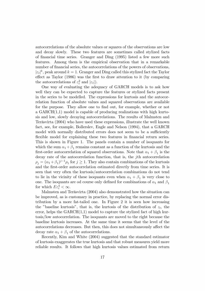
autocorrelations of the absolute values or squares of the observations are lowand decay slowly. These two features are sometimes called stylized factsof �nancial time series. Granger and Ding (1995) listed a few more suchfeatures. Among them is the empirical observation that in a remarkablenumber of �nancial series, the autocorrelations of the powers of observations,j"tjk, peak around k = 1:Granger and Ding called this stylized fact the Taylore¤ect as Taylor (1986) was the �rst to draw attention to it (by comparingthe autocorrelations of "2t and j"tj):One way of evaluating the adequacy of GARCH models is to ask how

well they can be expected to capture the features or stylized facts presentin the series to be modelled. The expressions for kurtosis and the autocor-relation function of absolute values and squared observations are availablefor the purpose. They allow one to �nd out, for example, whether or nota GARCH(1,1) model is capable of producing realizations with high kurto-sis and low, slowly decaying autocorrelations. The results of Malmsten andTeräsvirta (2004) who have used these expressions, illustrate the well knownfact, see, for example, Bollerslev, Engle and Nelson (1994), that a GARCHmodel with normally distributed errors does not seem to be a su¢ ciently�exible model for explaining these two features in �nancial return series.This is shown in Figure 1. The panels contain a number of isoquants forwhich the sum �1+�1 remains constant as a function of the kurtosis and the�rst-order autocorrelation of squared observations. Note that �1 + �1 is thedecay rate of the autocorrelation function, that is, the jth autocorrelation�j = (�1+�1)

j�1�1 for j � 1: They also contain combinations of the kurtosisand the �rst-order autocorrelation estimated directly from time series. It isseen that very often the kurtosis/autocorrelation combinations do not tendto lie in the vicinity of these isoquants even when �1 + �1 is very close toone. The isoquants are od course only de�ned for combinations of �1 and �1for which E"4t <1:Malmsten and Teräsvirta (2004) also demonstrated how the situation can

be improved, as is customary in practice, by replacing the normal error dis-tribution by a more fat-tailed one. In Figure 2 it is seen how increasingthe �baseline kurtosis�, that is, the kurtosis of the distribution of zt; theerror, helps the GARCH(1,1) model to capture the stylized fact of high kur-tosis/low autocorrelation. The isoquants are moved to the right because thebaseline kurtosis increases. At the same time it seems that the level of theautocorrelations decreases. But then, this does not simultaneously a¤ect thedecay rate �1 + �1 of the autocorrelations.Recently, Kim and White (2004) suggested that the standard estimator

of kurtosis exaggerates the true kurtosis and that robust measures yield morereliable results. It follows that high kurtosis values estimated from return

17

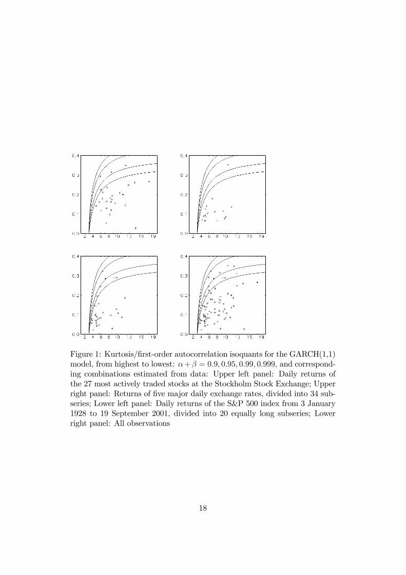
Figure 1: Kurtosis/�rst-order autocorrelation isoquants for the GARCH(1,1)model, from highest to lowest: �+� = 0:9; 0:95; 0:99; 0:999; and correspond-ing combinations estimated from data: Upper left panel: Daily returns ofthe 27 most actively traded stocks at the Stockholm Stock Exchange; Upperright panel: Returns of �ve major daily exchange rates, divided into 34 sub-series; Lower left panel: Daily returns of the S&P 500 index from 3 January1928 to 19 September 2001, divided into 20 equally long subseries; Lowerright panel: All observations

18

Figure 2: Isoquants of pairs of kurtosis and �rst-order autocorrelation ofsquared observations in the GARCH(1,1) model with t(7)-distributed (left-hand panel) and t(5)-distributed errors (right-hand panel), for (from above)�+� = 0:90; 0.95, 0.99 and 0.999, and corresponding observations (the sameones as in the lower right panel of Figure 1)

series are a result of a limited number of outliers. If this is the case, thenthe use of a non-normal (heavy-tailed) error distribution may not necessarilybe an optimal extension to the standard normal-error GARCH model. How-ever, Teräsvirta and Zhao (2006) recently studied 160 daily return series and,following Kim and White (2004), used robust kurtosis and autocorrelationestimates instead of standard ones. Their results indicate that leptokurticdistributions for zt are needed in capturing the kurtosis-autocorrelation styl-ized fact even when the in�uence of extreme observations is dampened bythe use of robust estimates.As to the Taylor e¤ect, He and Teräsvirta (1999a) de�ned a correspond-

ing theoretical property, the Taylor property, as follows. Let �(j"tjk; j"t�jjk)be the jth order autocorrelation of fj"tjkg: The stochastic process has theTaylor property when �(j"tjk; j"t�jjk) is maximized for k = 1 for j = 1; 2; :::. In practice, He and Teräsvirta (1999a) were able to �nd analytical re-sults for the AVGARCH(1,1) model, but they were restricted to compar-ing the �rst-order autocorrelations for k = 1 and k = 2. For this model,�(j"tj; j"t�1j) > �("2t ; "

2t�1) when the kurtosis of the process is su¢ ciently

high. The corresponding results for the standard GARCH(1,1) model (4)with p = q = 1 and normal errors are not available as the autocorrelationfunction of fj"tjg cannot be derived analytically. Simulations conducted byHe and Teräsvirta (1999a) showed that the GARCH(1,1) model probably

19

does not possess the Taylor property, which may seem disappointing. Butthen, the results of Teräsvirta and Zhao (2006) show that if the standard kur-tosis and autocorrelation estimates are replaced by robust ones, the evidenceof the Taylor e¤ect completely disappears. This stylized fact may thus be aconsequence of just a small number of extreme observations in the series.

4 Family of Exponential GARCH models

4.1 De�nition and properties

The Exponential GARCH (EGARCH) model is another popular GARCHmodel. Nelson (1991) who introduced it had three criticisms of the standardGARCH model in mind. First, parameter restrictions are required to ensurepositivity of the conditional variance at every point of time. Second, thestandard GARCH model does not allow an asymmetric response to shocks.Third, if the model is an IGARCH one, measuring the persistence is di¢ cultsince this model is strongly but not weakly stationary. Shocks may be viewedpersistent as the IGARCH process looks like a random walk. However, theIGARCH model with �0 > 0 is strictly stationary and ergodic, and when�0 = 0; the realizations collapse into zero almost surely, as already indicatedin Section 3.6. The second drawback has since been removed as asymmet-ric GARCH models such as GJR-GARCH (Glosten et al. (1993)) or smoothtransition GARCH have become available. A family of EGARCH(p; q) mod-els may be de�ned as in (2) with

lnht = �0 +

qXj=1

gj(zt�j) +

pXj=1

�j lnht�j: (33)

When gj(zt�j) = �jzt�j + j(jzt�jj � Ejzt�jj); j = 1; :::; q; (33) becomes theEGARCH model of Nelson (1991). It is seen from (33) that no parameter re-strictions are necessary to ensure positivity of ht: Parameters �j; j = 1; :::; q;make an asymmetric response to shocks possible.When gj(zt�j) = �j ln z

2t�j; j = 1; :::; q; (2) and (33) form the logarithmic

GARCH (LGARCH) model that Geweke (1986) and Pantula (1986) pro-posed. The LGARCH model has not become popular among practitioners.A principal reason for this may be that for parameter values encounteredin practice, the theoretical values of the �rst few autocorrelations of {"2tg atshort lags tend to be so high that such autocorrelations can hardly be foundin �nancial series such as return series. This being the case, the LGARCHmodel cannot be expected to provide an acceptable �t when applied to �-

20

nancial series. Another reason are the occasional small values of ln "2t thatcomplicate the estimation of parameters.As in the standard GARCH case, the �rst-order model is the most popu-

lar EGARCH model in practice. Nelson (1991) derived existence conditionsfor moments of the general in�nite-order Exponential ARCH model. Trans-lated to the case of the EGARCH model (2) and (33) such that gj(zt�j) =�jzt�j + j(jzt�jj � Ejzt�jj), j = 1; :::; q; where not all �j and j equalzero, the conditions imply that if the error process {ztg has all moments andPp

j=1 �2j < 1 in (33), then all moments for the EGARCH process {"tg exist.

For example, if {ztg is a sequence of independent standard normal variablesthen the restrictions on �j; j = 1; :::; p; are necessary and su¢ cient for theexistence of all moments simultaneously. This is di¤erent from the family(12) of GARCH models considered in Section 3.2. For those models, the mo-ment conditions become more and more stringent for higher and higher evenmoments. The expressions for moments of the �rst-order EGARCH processcan be found in He, Teräsvirta and Malmsten (2002); for the more generalcase, see He (2000).

4.2 Stylized facts and the �rst-order EGARCH model

In Section 3.9 we considered the capability of �rst-order GARCH models tocharacterize certain stylized facts in �nancial time series. It is instructive todo the same for EGARCH models. For the �rst-order EGARCH model, thedecay of autocorrelations of squared observations is faster than exponential inthe beginning before it slows down towards an exponential rate; see He et al.(2002). Thus it does not appear possible to use a standard EGARCH(1,1)model to characterize processes with very slowly decaying autocorrelations.Malmsten and Teräsvirta (2004) showed that the symmetric EGARCH(1,1)model with normal errors is not su¢ ciently �exible either for characterizingseries with high kurtosis and slowly decaying autocorrelations. As in thestandard GARCH case, assuming normal errors means that the �rst-orderautocorrelation of squared observations increases quite rapidly as a functionof kurtosis for any �xed �1 before the increase slows down. Analogouslyto GARCH, the observed kurtosis/autocorrelation combinations cannot bereached by the EGARCH(1,1) model with standard normal errors. The asym-metry parameter is unlikely to change things much.Nelson (1991) recommended the use of the so-called Generalized Error

Distribution (GED) for the errors. It contains the normal distribution as aspecial case but also allows heavier tails than the ones in the normal distri-bution. Nelson (1991) also pointed out that a t-distribution for the errorsmay imply in�nite unconditional variance for {"tg: As in the case of the

21

GARCH(1,1) model, an error distribution with fatter tails than the normalone helps to increase the kurtosis and, at the same time, lower the autocor-relations of squared observations or absolute values.Because of analytical expressions of the autocorrelations for k > 0 given

in He et al. (2002) it is possible to study the existence of the Taylor propertyin EGARCH models. Using the formulas for the autocorrelations of {j"tjkg;k > 0; it is possible to �nd parameter combinations for which these autocor-relations peak in a neighbourhood of k = 1. A subset of �rst-order EGARCHmodels thus has the Taylor property. This subset is also a relevant one inpractice in the sense that it contains EGARCH processes with the kurtosis ofthe magnitude frequently found in �nancial time series. For more discussionon stylized facts and the EGARCH(1,1) model, see Malmsten and Teräsvirta(2004).

4.3 Stochastic volatility

The EGARCH equation may be modi�ed by replacing gj(zt�j) by gj(st�j)where {stg is a sequence of continuous unobservable independent randomvariables that are often assumed independent of zt at all lags. Typically inapplications, p = q = 1 and g1(st�1) = �st�1 where � is a parameter to beestimated: This generalization is called the autoregressive stochastic volatil-ity (SV) model, and it substantially increases the �exibility of the EGARCHparameterization. For evidence of this, see Malmsten and Teräsvirta (2004)and Carnero, Peña and Ruiz (2004). A disadvantage is that model evalua-tion becomes more complicated than that of EGARCH models because theestimation does not yield residuals. Several articles in this Handbook aredevoted to SV models.

5 Comparing EGARCH with GARCH

The standard GARCH model is probably the most frequently applied pa-rameterization of conditional heteroskedasticity. This being the case, it isnatural to evaluate an estimated EGARCH model by testing it against thecorresponding GARCH model. Since the EGARCH model can characterizeasymmetric responses to shocks, a GARCH model with the same property,such as the GJR-GARCH or the smooth transition GARCH model, wouldbe a natural counterpart in such a comparison. If the aim of the comparisonis to choose between these models, they may be compared by an appropriatemodel selection criterion as in Shephard (1996). Since the GJR-GARCH andthe EGARCH model of the same order have equally many parameters, this

22

amounts to comparing their maximized likelihoods.If the investigator has a preferred model or is just interested in knowing

if there are signi�cant di¤erences in the �t between the two, the models maybe tested against each other. The testing problem is a non-standard onebecause the two models do not nest each other. Several approaches havebeen suggested for this situation. Engle and Ng (1993) proposed combiningthe two models into an encompassing model. If the GARCHmodel is an GJR-GARCH(p; q) one (both models can account for asymmetries), this leads tothe following speci�cation of the conditional variance:

lnht =

qXj=1

f��jzt�j + �j(jzt�jj � Ejzt�jj)g+pXj=1

��j lnht�j

+ ln(�0 +

qXj=1

f�j + !jI("t�j)g"2t�j +pXj=1

�jht�j): (34)

Setting (�j; !j) = (0; 0); j = 1; :::; q; and �j = 0; j = 1; :::; p; in (34) yieldsan EGARCH(p; q) model. Correspondingly, the restrictions (��j ;

�j) = (0; 0);

j = 1; :::; q; and ��j = 0; j = 1; :::; p; de�ne the GJR-GARCH(p; q) model.Testing the models against each other amounts to testing the appropriaterestrictions in (34) : A Lagrange Multiplier test may be constructed for thepurpose. The test may also be viewed as another misspeci�cation test andnot only as a test against the alternative model.Another way of testing the EGARCH model against GARCH consists of

forming the likelihood ratio statistic despite the fact that the null model isnot nested in the alternative. This is discussed in Lee and Brorsen (1997) andKim, Shephard and Chib (1998). LetM0 be the EGARCH model andM1

the GARCH one, and let the corresponding log-likelihoods be LT (";M0;�0)and LT (";M1;�1); respectively. The test statistic is

LR = 2fLT (";M1; b�1)� LT (";M0; e�0)g: (35)

The asymptotic null distribution of (35) is unknown but can be approxi-mated by simulation. Assuming that the EGARCH model is the null modeland that e�0 is the true parameter, one generates N realizations of T obser-vations from this model and estimates both models and calculates the valueof (35) using each realization. Ranking the N values gives an empirical dis-tribution with which one compares the original value of (35) : The true valueof �0 is unknown, but the approximation error due to the use of e�0 as areplacement vanishes asymptotically as T !1. If the value of (35) exceedsthe 100(1� �)% quantile of the empirical distribution, the null model is re-jected at signi�cance level �: Note that the models under comparison need

23

not have the same number of parameters, and the value of the statistic canalso be negative. Reversing the roles of the models, one can test GARCHmodels against EGARCH ones.Chen and Kuan (2002) proposed yet another method based on the pseudo-

score, whose estimator under the null hypothesis and assuming the custom-ary regularity conditions is asymptotically normally distributed. This resultforms the basis for a �2-distributed test statistic; see Chen and Kuan (2002)for details.Results of small-sample simulations in Malmsten (2004) indicate that

the pseudo-score test tends to be oversized. Furthermore, the Monte Carlolikelihood ratio statistic seems to have consistently higher power than theencompassing test, which suggests that the former rather than the lattershould be applied in practice.

6 Final remarks and further reading

The literature on univariate GARCH models is quite voluminous, and it isnot possible to incorporate all developments and extensions of the originalmodel in the present text. Several articles of this Handbook provide detailedanalyses of various aspects of GARCH models. Modern econometrics textscontain accounts of conditional heteroskedasticity. A number of surveys ofGARCH models exist as well. Bollerslev et al. (1994), Diebold and Lopez(1995), Palm (1996), and Guégan (1994, Ch. 5), survey developments tillthe early 1990s; see Giraitis, Leipus and Surgailis (2006) for a very recentsurvey. Shephard (1996) considers both univariate GARCH and stochasticvolatility models. The focus in Gouriéroux (1996) lies on both univariateand multivariate ARCH models. The survey by Bollerslev et al. (1992) alsoreviews applications to �nancial series. The focus in Straumann (2004) is onestimation in models of conditional heteroskedasticity. Theoretical results ontime series models with conditional heteroskedasticity are also reviewed inLi, Ling and McAleer (2002). Engle (1995) contains a selection of the mostimportant articles on ARCH and GARCH models up until 1993.Multivariate GARCHmodels are not included in this article. There exists

a recent survey by Bauwens, Laurent and Rombouts (2006), and these modelsare also considered in Silvennoinen and Teräsvirta (2007).

24

References

Andersen, T. G. and Bollerslev, T.: 1998, Answering the skeptics: Yes,standard volatility models provide accurate forecasts, International Eco-nomic Review 39, 885�905.

Anderson, H. M., Nam, K. and Vahid, F.: 1999, Asymmetric nonlinearsmooth transition GARCHmodels, in P. Rothman (ed.), Nonlinear timeseries analysis of economic and �nancial data, Kluwer, Boston, pp. 191�207.

Audrino, F. and Bühlmann, P.: 2001, Tree-structured generalized autoregres-sive conditional heteroscedastic models, Journal of the Royal StatisticalSociety B 63, 727�744.

Baillie, R. T., Bollerslev, T. and Mikkelsen, H. O.: 1996, Fractionally inte-grated generalized autoregressive conditional heteroskedasticity, Journalof Econometrics 74, 3�30.

Bauwens, L., Laurent, S. and Rombouts, J. V. K.: 2006, MultivariateGARCH models: A survey, Journal of Applied Econometrics 21, 79�109.

Bollerslev, T.: 1986, Generalized autoregressive conditional heteroskedastic-ity, Journal of Econometrics 31, 307�327.

Bollerslev, T., Chou, R. Y. and Kroner, K. F.: 1992, ARCH modeling in �-nance. A review of the theory and empirical evidence, Journal of Econo-metrics 52, 5�59.

Bollerslev, T., Engle, R. F. and Nelson, D. B.: 1994, ARCH models, in R. F.Engle and D. L. McFadden (eds), Handbook of Econometrics, Vol. 4,North-Holland, Amsterdam, pp. 2959�3038.

Cai, J.: 1994, A Markov model of switching-regime ARCH, Journal of Busi-ness and Economic Statistics 12, 309�316.

Carnero, M. A., Peña, D. and Ruiz, E.: 2004, Persistence and kurtosis inGARCH and stochastic volatility models, Journal of Financial Econo-metrics 2, 319�342.

Chen, Y.-T. and Kuan, C.-M.: 2002, The pseudo-true score encompassingtest for non-nested hypotheses, Journal of Econometrics 106, 271�295.

25

Chu, C.-S. J.: 1995, Detecting parameter shift in GARCH models, Econo-metric Reviews 14, 241�266.

Davidson, J.: 2004, Moment and memory properties of linear conditionalheteroscedasticity models, and a new model, Journal of Business andEconomic Statistics 22, 16�29.

Diebold, F. X.: 1986, Modeling the persistence of conditional variances: Acomment, Econometric Reviews 5, 51�56.

Diebold, F. X. and Lopez, J. A.: 1995, Modeling volatility dynamics, inK. D. Hoover (ed.), Macroeconometrics: Developments, Tensions, andProspects, Kluwer, Boston, pp. 427�472.

Ding, Z., Granger, C. W. J. and Engle, R. F.: 1993, A long memory propertyof stock market returns and a new model, Journal of Empirical Finance1, 83�106.

Duan, J.-C.: 1997, Augmented GARCH(p,q) process and its di¤usion limit,Journal of Econometrics 79, 97�127.

Engle, R. F.: 1982, Autoregressive conditional heteroscedasticity with es-timates of the variance of United Kingdom in�ation, Econometrica50, 987�1007.

Engle, R. F.: 2004, Risk and volatility: Econometric models and �nancialpractice, American Economic Review 94, 405�420.

Engle, R. F. and Bollerslev, T.: 1986, Modeling the persistence of conditionalvariances, Econometric Reviews 5, 1�50.

Engle, R. F. (ed.): 1995, ARCH. Selected Readings, Oxford University Press,Oxford.

Engle, R. F., Lilien, D. M. and Robins, R. P.: 1987, Estimating time-varyingrisk premia in the term structure: The ARCH-M model, Econometrica55, 391�407.

Engle, R. F. and Mezrich, J.: 1996, GARCH for groups, Risk 9(8), 36�40.

Engle, R. F. and Ng, V. K.: 1993, Measuring and testing the impact of newson volatility, Journal of Finance 48, 1749�1777.

Friedman, M.: 1977, Nobel lecture: In�ation and unemployment, Journal ofPolitical Economy 85, 451�472.

26

Geweke, J.: 1986, Modeling the persistence of conditional variances: A com-ment, Econometric Reviews 5, 57�61.

Giraitis, L., Kokoszka, P. and Leipus, R.: 2000, Stationary ARCH models:Dependence structure and central limit theorem, Econometric Theory16, 3�22.

Giraitis, L., Leipus, R. and Surgailis, D.: 2006, Recent advances in ARCHmodelling, in A. Kirman and G. Teyssiere (eds), Long Memory in Eco-nomics, Springer, Berlin.

Glosten, L., Jagannathan, R. and Runkle, D.: 1993, On the relation betweenexpected value and the volatility of the nominal excess return on stocks,Journal of Finance 48, 1779�1801.

Gonzalez-Rivera, G.: 1998, Smooth transition GARCH models, Studies inNonlinear Dynamics and Econometrics 3, 161�178.

Gouriéroux, C.: 1996, ARCH Models and Financial Applications, Springer,Berlin.

Granger, C. W. J. and Ding, Z.: 1995, Some properties of absolute returns.An alternative measure of risk, Annales d�économie et de statistique40, 67�92.

Gray, S. F.: 1996, Modeling the conditional distribution of interest rates asa regime-switching process, Journal of Financial Economics 42, 27�62.

Guégan, D.: 1994, Séries chronologiques non linéaires à temps discret, Eco-nomica, Paris.

Haas, M., Mittnik, S. and Paolella, M. S.: 2004, A new approach to Markov-switching GARCH models, Journal of Financial Econometrics 4, 493�530.

Hagerud, G.: 1997, A New Non-Linear GARCH Model, EFI Economic Re-search Institute, Stockholm.

Hamilton, J. D. and Susmel, R.: 1994, Autoregressive conditional het-eroskedasticity and changes in regime, Journal of Econometrics 64, 307�333.

He, C.: 2000, Moments and the autocorrelation structure of the exponentialGARCH(p; q) process., SSE/EFI Working Paper Series in Economicsand Finance 359, Stockholm School of Economics.

27

He, C., Silvennoinen, A. and Teräsvirta, T.: 2006, Parameterizing uncondi-tional skewness in models for �nancial time series, Unpublished paper,Stockholm School of Economics.

He, C. and Teräsvirta, T.: 1999a, Properties of moments of a family ofGARCH processes, Journal of Econometrics 92, 173�192.

He, C. and Teräsvirta, T.: 1999b, Properties of the autocorrelation functionof squared observations for second order GARCH processes under twosets of parameter constraints, Journal of Time Series Analysis 20, 23�30.

He, C., Teräsvirta, T. and Malmsten, H.: 2002, Moment structure of a familyof �rst-order exponential GARCHmodels, Econometric Theory 18, 868�885.

Hentschel, L.: 1995, All in the family. Nesting symmetric and asymmetricGARCH models, Journal of Financial Economics 39, 71�104.

Hong, E. P.: 1991, The autocorrelation structure for the GARCH-M process,Economics Letters 37, 129�132.

Kim, S., Shephard, N. and Chib, S.: 1998, Stochastic volatility: Likeli-hood inference and comparison with ARCHmodels, Review of EconomicStudies 65, 361�393.

Kim, T.-H. and White, H.: 2004, On more robust estimation of skewnessand kurtosis, Finance Research Letters 1, 56�73.

Klaassen, F.: 2002, Improving GARCH volatility forecasts with regime-switching GARCH, Empirical Economics 27, 363�394.

Lamoureux, C. G. and Lastrapes, W. G.: 1990, Persistence in variance, struc-tural change and the GARCHmodel, Journal of Business and EconomicStatistics 8, 225�234.

Lange, T. and Rahbek, A.: 2007, An introduction to regime switching timeseries, in T. G. Andersen, R. A. Davis, J.-P. Kreiss and T. Mikosch(eds), Handbook of Financial Time Series, Springer, New York.

Lanne, M. and Saikkonen, P.: 2005, Nonlinear GARCH models for highlypersistent volatility, Econometrics Journal 8, 251�276.

Lee, J.-H. and Brorsen, B. W.: 1997, A non-nested test of GARCH vs.EGARCH models, Applied Economics Letters 4, 765�768.

28

Li, C. W. and Li, W. K.: 1996, On a double threshold autoregressiveheteroskedasticity time series model, Journal of Applied Econometrics11, 253�274.

Li, W. K., Ling, S. and McAleer, M.: 2002, Recent theoretical results fortime series models with GARCH errors, Journal of Economic Surveys16, 245�269.

Linton, O.: 2007, Semi- and nonparametric ARCH/GARCH-Modelling, inT. G. Andersen, R. A. Davis, J.-P. Kreiss and T. Mikosch (eds), Handookof Financial Time Series, Springer, New York.

Liu, J.-C.: 2006, Stationarity of a Markov-switching GARCH model, Journalof Financial Econometrics 4, 573�593.

Malmsten, H.: 2004, Evaluating Exponential GARCH models, SSE/EFIWorking Paper Series in Economics and Finance 564, Stockholm Schoolof Economics.

Malmsten, H. and Teräsvirta, T.: 2004, Stylized facts of �nancial time seriesand three popular models of volatility, SSE/EFI Working Paper Seriesin Economics and Finance 563, Stockholm School of Economics.

Mandelbrot, B.: 1963, The variation of certain speculative prices, Journal ofBusiness 36, 394�419.

Mandelbrot, B. and Taylor, H.: 1967, On the distribution of stock pricedi¤erences, Operations Research 15, 1057�1062.

Mikosch, T. and Starica, C.: 2004, Nonstationarities in �nancial time se-ries, the long-range dependence, and the IGARCH e¤ects, Review ofEconomics and Statistics 86, 378�390.

Nelson, D. B.: 1991, Conditional heteroskedasticity in asset returns: A newapproach, Econometrica 59, 347�370.

Nelson, D. B. and Cao, C. Q.: 1992, Inequality constraints in the univariateGARCH model, Journal of Business and Economic Statistics 10, 229�235.

Palm, F. C.: 1996, GARCH models of volatility, in G. Maddala and C. Rao(eds), Handbook of Statistics: Statistical Methods in Finance, Vol. 14,Elsevier, Amsterdam, pp. 209�240.

29

Pantula, S. G.: 1986, Modeling the persistence of conditional variances: Acomment, Econometric Reviews 5, 71�74.

Rabemananjara, R. and Zakoïan, J. M.: 1993, Threshold ARCH models andasymmetries in volatility, Journal of Applied Econometrics 8, 31�49.

Rachev, S. and Mittnik, S.: 2000, Stable Paretian Models in Finance, Wiley,Chichester.

Rydén, T., Teräsvirta, T. and Åsbrink, S.: 1998, Stylized facts of daily returnseries and the hidden Markov model, Journal of Applied Econometrics13, 217�244.

Schwert, G. W.: 1990, Stock volatility and the crash of �87, Review of Fi-nancial Studies 3, 77�102.

Sentana, E.: 1995, Quadratic ARCH models, Review of Economic Studies62, 639�661.

Shephard, N. G.: 1996, Statistical aspects of ARCH and stochastic volatility,in D. R. Cox, D. V. Hinkley and O. E. Barndor¤-Nielsen (eds), TimeSeries Models. In Econometrics, Finance and Other Fields, Chapmanand Hall, London, pp. 1�67.

Silvennoinen, A. and Teräsvirta, T.: 2007, Multivariate GARCH models,in T. G. Andersen, R. A. Davis, J.-P. Kreiss and T. Mikosch (eds),Handbook of Financial Time Series, Springer, New York.

Straumann, D.: 2004, Estimation in Conditionally Heteroscedastic Time Se-ries Models, Springer, New York.

Taylor, S.: 1986, Modelling Financial Time Series, Wiley, Chichester.

Teräsvirta, T. and Zhao, Z.: 2006, Stylized facts of return series, robustestimates, and three popular models of volatility, Unpublished paper,Stockholm School of Economics.

Tong, H.: 1990, Non-Linear Time Series. A Dynamical System Approach,Oxford University Press, Oxford.

Zakoïan, J.-M.: 1994, Threshold heteroskedastic models, Journal of Eco-nomic Dynamics and Control 18, 931�955.

30