an introduction to winbugs and boa. outline zintroduction zquick review of bayesian statistical...
Post on 21-Dec-2015
220 views
TRANSCRIPT

An Introduction to WinBUGS and BOA

Outline
Introduction Quick review of Bayesian statistical analysis The WinBUGS language Convergence diagnostics and BOA (Bayesian
Output Analysis).
Illustration with example --- Meta - analysis

Introduction
What is WinBUGS? joint endeavor between the MRC Biostatistics
Unit in Cambridge and the Department of Epidemiology and Public Health of Imperial College, at St Mary's Hospital London
BUGS: Bayesian Inference Using Gibbs Sampling
WinBUGS: DoodleBUGS (graphical representation of model) and window interface
for controlling the analysis.

Introduction
WinBUGS can handle analysis for complex statistical models Missing data Measurement error No closed form for posterior distribution
Bayesian posterior inference achieved via Markov chain Monte Carlo (MCMC) Integration Useful when no closed form exists.

Bayesian Inference
Suppose we have data x , and unknowns which might be model parameters missing data events we did not observe directly or exactly (e. g.,
latent variables)
Bayesian approach concerns making statements about given data x.
Recall Bayes theorem:
)|()(
)|()()|()(
arg
xpp
dxppxpp
inalmlikelihoodprior
Posterior

Bayesian Inference Components of Bayesian inference
The prior distribution p(). Use probability as means of quantifying uncertainty about before taking into account the data.
The likelihood p(x|). Relate all variables into a “full probability model”.
The posterior distribution p(|x). Express uncertainty about
after taking into account the data. Utilities --- required for decision making and not discussed here.
Given a posterior distribution p(|x), we may want mean, standard deviations, medians etc. probability of exceeding certain thresholds, p( > 0|x). Inference on arbitrary functions of unknown model parameters.
And they are easily to be implemented in WinBUGS.

Priors Where does the prior come from?
It is in principle subjective. It might be elicited from experts. It might be more convincing to be based on existing
data. But the assumed relevance is still a subjective judgement.
There are various “objective” approaches. Conjugacy is useful but no longer necessary. It might be assumed unknown (full Bayes) or
“estimated” (Empirical Bayes). “Non-informative” priors

Priors “ Non-informative” priors
also known as vague, ignorance, flat, diffuse and so on There could exist a prior that reproduces the classical
results. Often improper. Usually quite unrealistic. However, always useful to report likelihood-based results
as arising from a ‘reference’ prior. WinBUGS does not allow improper priors. General idea: by sensitivity analysis to a community of
priors, one can assess whether the current results will be convincing to a broad spectrum of opinion.

Bayesian Inference
Probabilities of parameters are based on all available information.
Some theoretical advantages (Spiegelhalter D. 1999) Only need probability theory as basis for inference. No need to worry about statistical ‘principles’ such as:
unbiasedness, efficiency, sufficiency, ancillarity, consistency, asymptotics and so on.
No need to worry about significance tests, stopping rules, p - values.
Models can be as complex as reality demands (But WinBUGS still has its limitations).
Integrates with planning decisions. Tell us what is desired: how should this piece of evidence
change what we currently believe?

Bayesian Inference
Some practical difficulties (Spiegelhalter D. 1999) Inferences need to be justified to an outside world
(reviewers, regulatory bodies, the public and so on): in particular
Where did the prior come from?Is the model for the data appropriate (standard diagnostics)?If making decisions, whose utilities?
Although huge progress has been made, computational problems can still be considerable.
Cannot overcome basic deficiencies in design. Standards are needed for Bayesian analysis and reporting.

MCMC --- To Achieve Bayesian Inference
MCMC --- Markov chain Monte Carlo. Usually we are interested in studying a vector of
unknown , say, with k components and the posterior distribution for or components of might not be able to simplify to known distribution forms.
Remedy: Sampling from a Markov chain with p( |x) as its stationary
distribution. Gibbs Sampling: sampling from full conditional distribution
p(j|1,…,j-1,j+1,…k , x) Methods have been developed to implement sampling.

Sampling methods used in WinBUGS
The sampling methods are used in the following hierarchies:
Continuous targetdistribution
Method
Conjugate Direct sampling using standard algorithms
Log-concave Derivative - free adaptive rejection sampling(Gilks, 1992)
Restricted range Slice sampling (Neal, 1997)
Unrestricted range Current point Metropolis
Discrete targetdistribution
Method
Finite upper bound Inversion
Shifted poisson Direct sampling using standard algorithm

MCMC --- To Achieve Bayesian Inference
Inference may be achieve via Monte Carlo integration. Monte Carlo integration
Suppose we can draw samples from the joint posterior distribution for , i.e. (1), (2), …, (n) ~ p( |x)
Then
Result: really easy to make inference on an arbitrary function of parameters!!
)(1
)|()())((
)(
1
in
ig
n
dxpggE
Bayesian Graphical Modeling
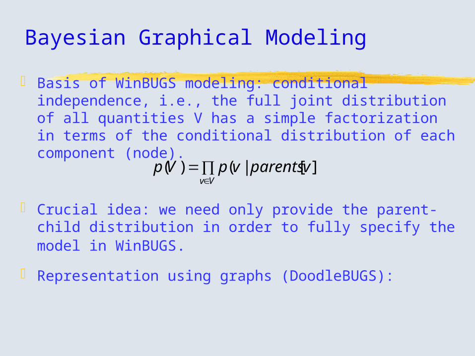
Basis of WinBUGS modeling: conditional independence, i.e., the full joint distribution of all quantities V has a simple factorization in terms of the conditional distribution of each component (node).
Crucial idea: we need only provide the parent-child distribution in order to fully specify the model in WinBUGS.
Representation using graphs (DoodleBUGS):
Vv
vparentsvpVp ])[|()(

Recap: Bayesian inference
Bayesian inference is based on the posterior distribution, which is derived from prior distribution and likelihood through Bayes theorem.
Bayesian inference is achieved through Monte Carlo integration where samples of posterior distribution can be obtained from MCMC simulation.

Analysis using WinBUGS
Three basic parts of a WinBUGS file: Model specification
BUGS language: Similar to S - Plus.Graphical language: Using DoodleBUGS
• It is good practice to construct a directed graphical model to communicate the structure of the problem.
• However, there are some features in BUGS language that could not be represented by DoodleBUGS. Examples of DoodleBUGS are given but no more details.
• For tutorial purpose, see http://www.mrc-bsu.cam.ac.uk/bugs/winbugs/winbugs-demo.pdf for “WinBUGS Demo” and “Doodle help” in WinBUGS13 help.
Data Initial values for unknowns .

Expressing model in the BUGS language Lexical conventions
Quantity (node) names. Characters: letters, numbers and period.Starting with a letter, not ending with a period.Upper or lower case or mixed, but case is important.Length restriction: 32 characters.
IndexingVectors and matrices are indexed within square brackets [..].No limitation on dimensionality of arrays.
NumbersStandard or exponential notation.A decimal point must be included in the exponential format.Legal notion for 0.0001: .0001, 0.0001, 1.0E-4, 1.0e-4, 1.E-4, 1.0E-
04, but NOT 1E-4.

Expressing model in the BUGS language
Model statementmodel{ text-based statements to describe model in BUGS
language}
Arbitrary spaces may be used in statements. Multiple statements may appear in a single line as well as
one statement may extend over several lines. Comment line is followed by a #.

Expressing model in the BUGS language
Model description Constant: fixed by the design of study. Stochastic nodes: variables (data or parameters) that
are given a distribution x ~ dbin(p,n)
where ~ means “distributed as”.The parameters of a distribution must be explicit. Scalar
parameters can be numerical constants but function expressions are not allowed.
Currently, WinBUGS could handle 20 distributions.(See Appendix A, Table I)

Expressing model in the BUGS language
Model description (cont.) Deterministic nodes: logical functions of other nodes.
pred <- beta0 + beta1 * xor Log(p) <-
where <- means “to be replaced by”.Can not be given initial values or data except for data
transformation facility (discussed below).Logical expressions can be built using: +, – , * , / and
unitary minus.Functions in Table II (Appendix B) could also be used in
logical expressions.

Expressing model in the BUGS language
for loops Allow repetitive structures to be concisely
described. Same syntax as that of S - plus:
for (name in expression1:expression2) {
statements }
The two expressions need to be evaluated to be fixed integer quantities.
Possibly as functions using + – * /.
Expressing model in the BUGS language
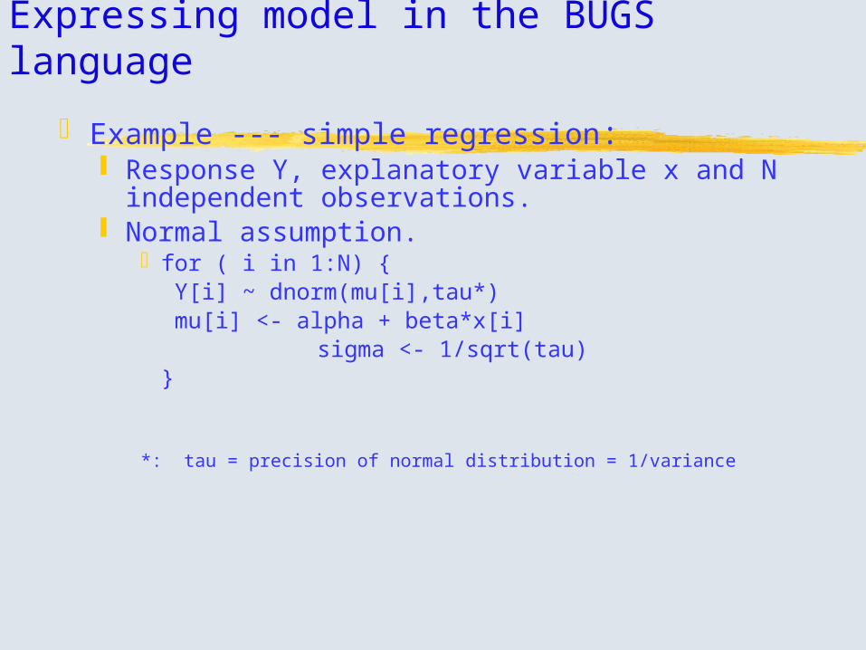
Example --- simple regression: Response Y, explanatory variable x and N
independent observations. Normal assumption.
for ( i in 1:N) { Y[i] ~ dnorm(mu[i],tau*) mu[i] <- alpha + beta*x[i]
sigma <- 1/sqrt(tau)}
*: tau = precision of normal distribution = 1/variance

Example of graphical modeling
for(i IN 1 : N)
sigma
taubetaalpha
mu[i]
Y[i]Y[i]
name: Y[i] type: stochastic density: dnormmean mu[i] precision tau lower bound upper bound
Ellipses: stochastic or deterministic node solid arrow: a stochastic dependence hollow arrow: a logical function. Plate: repeated structure

More on Stochastic nodes
Multivariate Nodes Using distributions unlisted in Table I. Censoring and truncation

More on Stochastic nodes Multivariate Nodes
Dirichlet, multinomial, multivariate normal and Wishart.
Contiguous elements: Multivariate nodes must form contiguous elements in an array. For example, to define a set of 3-dim multivariate normal variables x as a bidimensional array, we could write:
for (i in 1:K) {X[i,1:3] ~dmnorm (mu[1:3], prec[1:3,1:3])}
No missing data: missing values are not allowed in data defined as multivariate normal or multinomial.
Possible remedy: re-express the multivariate likelihood as a sequence of conditional univariate normal or binomial distributions.

More on Stochastic nodes
Multivariate Nodes (cont.) Conjugate updating:
Dirichlet: only as prior (parent) of multinomial probs.Wishart: only as prior (parent) of multivariate normal
precision matrix.Parameters of Dirichlet and Wishart must be specified
explicitly and can not be given prior distribution. Structured precision matrices for multivariate normals:
If a Wishart prior is not used for the precision matrix of a multivariate node, then the elements of the precision matrix are updated univariately and it is the user’s responsibility to specify a positive-definite matrix.

More on Stochastic nodes
Using distributions unlisted in Table I. Suppose data y is a vector of length n and for
unknown , it is desired to fit the model p (y) = f (y, ) and f is the formula of the density that is not currently handled by BUGS, the following trick could be used:
for (i in 1:n) {ones[i] <- 1ones[i] <- dbern(p[i])p[i] <- f (y[i], ) / K
}Where K is a sufficiently large constant to ensure p[i] <- 1.

More on Stochastic nodes Censoring and truncation
Censoringinterval censored: y ~ ddist()I(lower, upper)right censored: y ~ ddist()I(lower,)left censored: y ~ ddist()I(, upper)
For unknown , the sampling will only be correct if the bounds are conditionally independent of given y.
This construct should NOT be used for modeling truncated distribution. Truncated distribution may be handled by working out a usually complex algebraic form for the likelihood and using the technique for arbitrary distributions just discussed.
Check: If you knew y, would knowing (lower, upper) tell you anything further about ? --- Yes so, inappropriate construct of I.
More on Model specification
The declarative structure of model specification in BUGS language requires each node appears once and only once on the left hand side of a node.
Data transformation is the only exception. Indexing

More on Model specification
Data transformation Suppose we have data y and want to model , the following
statements could be used:for (i in 1:N) {
z[i] <- sqrt(y[i])
z[i] ~ dnorm(mu, tau)
}
Advantage: No need to create a separate variable in data.
No missing data is allowed. Example: leuk; endo
y
yz

More on Model specification
Indexing Functions as an index
+ – * / and appropriate bracketing. e.g. y[(I+J)*K]On the left hand side of a relation, a constant or a
function of data that always evaluates to a fixed value is allowed.
On the right hand side of a relation, a fixed value or a named node (nested indexing) is allowed.
No function of unobserved nodes allowed.• Intermediate deterministic nodes.
Implicit indexing: broadly following conventions of S - plus. n:m represents n, n+1 ,..., m . x[] represents all values of a vector x.y[,3] indicates all values of the third column of a two-dimensional
array y.

More on Model specification Indexing (cont.)
Nested indexingcan be very effective. e.g., suppose there are N studies and each study have
different number of treatments, S[N] is a vector contains information about the treatments across studies. Then “treatment” coefficients beta[I] can be declared and fitted using beta[S[i]] in a regression model.
Example: eyes.
Multidimensional arrays are handled as one-dimensional arrays with a constructed index. Thus functions defined on arrays must be over equally spaced nodes within an array: for example sum(i,1:4,k) .

Data and Initial Values Files Formatting of data.
S - plus format or rectangular format.S - plus format
• Scalars and arrays are named and given values in a single structure.
• Headed by Keyword list. There must be no space after list. • Example:
list(xbar = 22, N = 30, T = 5,
x = c(8.0, 15.0, 22.0, 29.0, 36.0),
Y = structure(.Data =
c(151, 199, 246, 283, 320,
145, 199, 249, 293, 354,
..........
137, 180, 219, 258, 291,
153, 200, 244, 286, 324),
.Dim = c(30,5) )
)

Data and Initial Values Files Formatting of data (cont.)
S - plus format or rectangular format.Rectangular format
• Headed by array name.• The array need to be of equal size.• The array names must have explicit brackets. • The first index position must be empty.• Example:
age[] sex[]
26 0
52 1
.…• Example of multi-dimensional arrays:
Y[,1] Y[,2] Y[,3] Y[,4] Y[,5]
151 199 246 283 320
145 199 249 293 354
....

Data and Initial Values Files Formatting of data (cont.).
S - plus format or rectangular format. The whole data must be specified in the file --- it is not
possible just to specify selected components. Missing values are represented as NA. All variables in a data file must be defined in a model. It is possible to load a mixture of rectangular and S -
plus format data for the same model. Initial values are specified following the same rules.

Example --- Meta Analysis
Problem: Lau et al. (1992) 33 trials evaluated the use of intravenous
streptokinase as thrombolyic therapy for myocardial infarction from 1959 to 1988.
Treatments: IV - SK vs. Placebo (Control).
Data: No. of death out of total subjects for each group.
Goal: Access the efficacy of IV - SK.

Example --- Meta AnalysisStudy Mortality: deaths (r) / total(n)
IV-SK PlaceboFletcher 1/12 4/11Dewar 4/21 7/21European_1 20/83 15/84European_2 69/373 94/357Heikinheimo 22/219 17/207Italian 19/164 18/157Australian 1 26/264 32/253Frankfurt_2 13/102 29/104NHLBI_SMIT 7/53 3/54Frank 6/55 6/53Valere 11/49 9/42Klein 4/14 1/9UK_Collab 38/302 40/293Austrian 37/352 65/376Australian 2 25/123 31/107Lasierra 1/13 3/11N_gerCollab 63/249 51/234
Study Mortality: deaths (r) / total(n)IV-SK Placebo
Witchitz 5/32 5/26European_3 18/156 30/159ISAM 54/859 63/882GissI-1 628/5860
758/5852Olson 1/28 2/24Baroffio 0/29 6/30Schreiber 1/19 3/19Cribier 1/21 1/23Sainsous 3/49 6/49Durand 3/35 4/29White 2/107 12/112Bassand 4/52 7/55Vlay 1/13 2/12Kennedy 12/191 17/177ISIS-2 791/8592
1029/8595Wisenberg 2/41 5/25

Example --- Meta Analysis A full Bayes Model.
Logistic regression. Measure of efficacy: difference of log-odds ratios. It is reasonable to assume the treatment effects from each trial
are similar but not exactly the same --- exchangeable. Exchangeability allows differences from study to study, but such
that the differences are not expected a priori to have predictable effects favoring one study or another,
Likelihood:
Placebo: riC ~ binomial (ni
C, piC)
IV - SK : riT ~ binomial (ni
T, piT)
logit(piC) = i
logit(piT) = i + i
Primary interest: i.

Example --- Meta Analysis A full Bayes Model(cont.).
Priors --- exchangeability
i ~ normal (d, )
i ~ normal (0, 1.0E-5)
Hyper priors
d ~ normal (0, 1.0E-6 )
~ gamma(0.001, 0.001)
“non-informative” priors are given for the 's, d and .
BUGS requires that a full probability model is defined, and hence forces all priors to be proper.
Not standard non-informative priors which usually are improper.

Example --- Meta Analysis
Likelihood:
riC ~ binomial (ni
C, piC)
riT ~ binomial (ni
T, piT)
logit(piC) = i
logit(piT) = i + i
Priors
i ~ normal (d, )
i ~ normal (0, 1.0E-5)
Hyper priors
d ~ normal (0, 1.0E-6 )
~ gamma(0.001, 0.001)
model
{
for( i in 1 : NoTrial) {
rc[i] ~ dbin(pc[i], nc[i])
rt[i] ~ dbin(pt[i], nt[i])
logit(pc[i]) <- mu[i]
logit(pt[i]) <- mu[i] + delta[i]
mu[i] ~ dnorm(0.0,1.0E-5)
delta[i] ~ dnorm(d, tau)
}
d ~ dnorm(0.0,1.0E-6)
tau ~ dgamma(0.001,0.001)
sigma <- 1 / sqrt(tau)
}
Specifying model in the BUGS language.

WinBUGS Demo
File: SK1.odc (Appendix C) Compound document --- nice interface
A file contains various types of information(formatted text, tables, plots, graphs etc) with special rectangular embedded regions or elements.
Each region could be manipulated by standard word-processing tools.
The Attributes menu: changes the style, size, font and color of the selected text.
The Text menu: changes the vertical offset of the selection. WinBUGS does not provided detailed information about how
to use these editing tools.

Running the Model in WinBUGS.
Under the Model Menu Click specification check model: Highlight the word
model in model statement and click the button “check model” to check the syntax of model.On the status line (lower left corner of screen) Model is syntactically correct. Or Error information.
load data: Highlight list (S - plus format) or the first array name (rectangular format) and click button to load data. Data Loaded. Error information.
check model load data
compile num of chains 1
load inits for chain 1
get inits

Running the Model in WinBUGS.
Under the Model Menu Click specification
Num of chains: Specify the number of chains to be simulated. The default number is one chain. Enter the number of chains desired
to be simulated. Multiple chains are needed for
convergence diagnostic. compile: Click to Build the data
structures needed to carry out Gibbs sampling. The model is checked for completeness and consistency with data. Model Compiled. Error information.
check model load data
compile num of chains 1
load inits for chain 1
get inits

Running the Model in WinBUGS. Under the Model Menu
Click specification
load inits: Click to load initial values of the nodes in the exactly same way as data.
gen inits: Generate initial values by sampling from the prior.
When specifying initial values, If some elements in an array are known, e.g.
constraints in a parameterization, those elements are specified as missing (NA) in the initial value files.
Initial values for each chain should be well dispersed. Generally it is recommended to load initial values for all
fixed effects model for all chains, initial values for random effects can be generated using the gen inits button.
Status line information: Initial values loaded: model contains uninitialized nodes
--- try gen inits. Initial values loaded: model initialized --- now model
ready to update. Error information.
check model load data
compile num of chains 1
load inits for chain 1
get inits
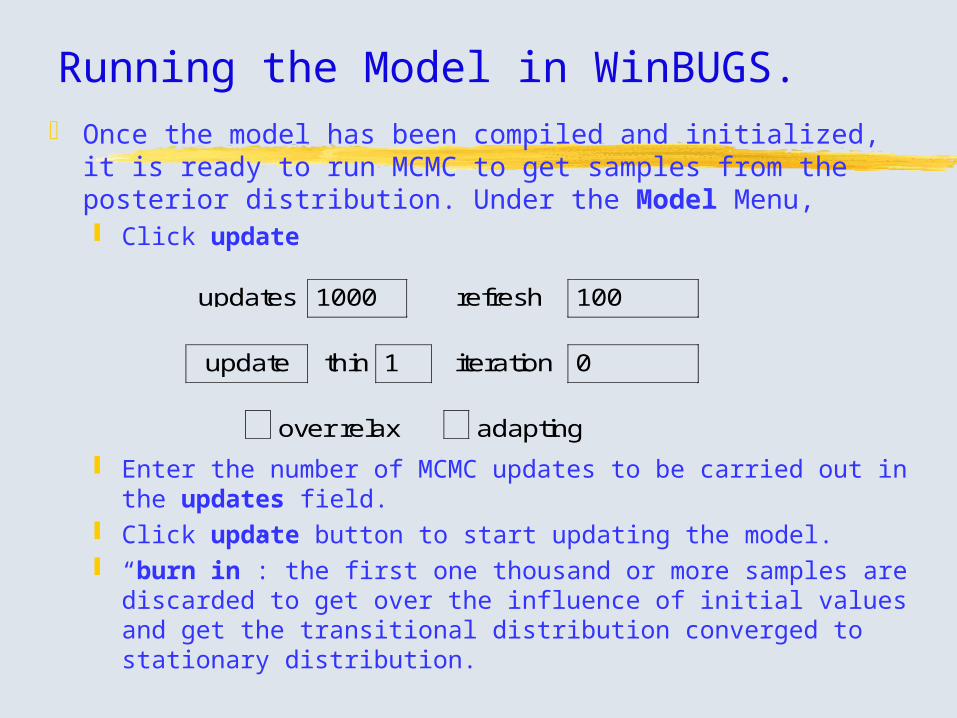
Running the Model in WinBUGS. Once the model has been compiled and initialized, it is ready to
run MCMC to get samples from the posterior distribution. Under the Model Menu, Click update
Enter the number of MCMC updates to be carried out in the updates field.
Click update button to start updating the model. “burn in”: the first one thousand or more samples are discarded to
get over the influence of initial values and get the transitional distribution converged to stationary distribution.
updates 1000 refresh 100
update thin 1 iteration 0
over relax adapting

Running the Model in WinBUGS. Other specifications about update.
refresh: the number of updates between redrawing the screen. thin: enter k in the field to store every kth iteration. No real
advantage except reducing storage requirement for very long run. over relax: In each iteration, generates multiple samples and
selects one that is negatively correlated with the current one. Reduce within chain autocorrelation not always effective.
adapting: indicates the initial tuning of Metropolis or slice-sampling algorithm. The first 4000 and 500 are discarded respectively.
updates 1000 refresh 100
update thin 1 iteration 0
over relax adapting

Bayesian Inference using WinBUGS
Under the Inference Menu and click Samplings:
Nodes: The variable of interest must be typed in this text field before updating to be monitored.
“ * “ serves as shorthand for all the stored samples. “deviance”, minus twice of log-likelihood is automatically calculated for
each iteration and can be monitored by typing in deviance.
set: click to finish the specification of interested variable.
Node chains 1 to 1 percentiles
beg 1 end 1000000 thin 1
clear set trace history density
stats coda quantiles GR diag autoC

Bayesian Inference using WinBUGS Under the Inference Menu and click Samplings:
beg and end: select a subset of the stored samples for analysis. chains and to: select chains for analysis. thin: select every kth iteration of each chain for analysis.
The sample for each chain are not independent. This dependence gets smaller when samples are getting further apart. Approximately independent samples could be obtained by checking the
autoC plot and looking for the appropriate lag.
Clear: removes the stored values of the variable.
Node chains 1 to 1 percentiles
beg 1 end 1000000 thin 1
clear set trace history density
stats coda quantiles GR diag autoC

Bayesian Inference using WinBUGS --- the meta-analysis example
Trace: dynamic plot of the variable value against iteration number. Redrawn each time when the the screen is redrawn.
d chains 3:1
iteration499004985049800
-1.0 -0.5 0.0 0.5 1.0
sigma chains 3:1
iteration499004985049800
0.0 1.0 2.0 3.0 4.0
delta[1] chains 3:1
iteration499004985049800
-3.0 -2.0 -1.0 0.0 1.0
delta[2] chains 3:1
iteration499004985049800
-1.5 -1.0 -0.5 0.0 0.5 1.0

Bayesian Inference using WinBUGS --- the meta-analysis example
quantiles: plots the running mean with running 95% confidence interval (credible set) against iteration number.
d chains 3:1
iteration10032 10200 10400 10600
-0.6 -0.5 -0.4 -0.3 -0.2 -0.1
sigma chains 3:1
iteration10032 10200 10400 10600
0.0 0.1 0.2 0.3 0.4
delta[1] chains 3:1
iteration10032 10200 10400 10600
-1.5
-1.0
-0.5
0.0delta[2] chains 3:1
iteration10032 10200 10400 10600
-1.5
-1.0
-0.5
0.0

Bayesian Inference using WinBUGS --- the meta-analysis example
History: complete trace of the variabled chains 1:3
iteration10000 20000 30000 40000
-0.8
-0.6
-0.4
-0.2
-5.55112E-17
sigma chains 1:3
iteration10000 20000 30000 40000
0.0
0.2
0.4
0.6

Bayesian Inference using WinBUGS --- the meta-analysis example
autoC: plots the autocorrelation function of the variable out to lag 50. Autocorrelation plot for every 10th sample.
d chains 1:3
lag0 20 40
-1.0 -0.5 0.0 0.5 1.0
sigma chains 1:3
lag0 20 40
-1.0 -0.5 0.0 0.5 1.0
delta[1] chains 1:3
lag0 20 40
-1.0 -0.5 0.0 0.5 1.0
delta[2] chains 1:3
lag0 20 40
-1.0 -0.5 0.0 0.5 1.0

Bayesian Inference using WinBUGS --- the meta-analysis example
More on autoC The autocorrelation
coefficient could be listed to a window by double-clicking on the plot followed by ctrl-left-mouse-click.
Helps to determine the thinning number of a chain to get independent samples.
Autocorrelation coefficient for d to lag 15 for 3 chains.
1 0.2887 0.3027 0.31022 0.1154 0.1181 0.15123 0.0398 0.07144 0.078874 0.0108 0.02785 0.065155 0.008905 0.02874 0.045986 0.009483 0.01345 0.042247 -0.007061 0.02338 0.036998 9.585E-4 0.007169 0.030519 -0.002919 -0.009028 0.0295810 0.00248 0.006675 0.0126711 0.004878 0.008473 0.0248812 -0.003961 0.006836 0.007014
13 -0.001721 0.004822 0.008959
14 0.002111 -0.004585 0.00799615 -0.002157 -0.008235 -0.01987

Bayesian Inference using WinBUGS --- the meta-analysis example
Autocorrelation coefficient for delta[1] to lag 15 for 3 chains.
1 0.07055 0.08014 0.14042 0.05591 0.05691 0.1073 0.006094 0.02561 0.05764 0.01724 0.02399 0.049935 0.001357 0.02152 0.023436 -0.008961 0.03044 0.030617 9.379E-4 -0.001046 -0.024198 -3.373E-5 -0.01555 -0.017279 -0.00459 -0.005384 0.0129810 0.005225 0.01231 -0.0183411 -0.005177 0.01187 -0.0138812 -5.76E-4 0.01402 -0.0159713 0.004723 -0.03354 0.0354614 -0.004878 -0.01139 0.019415 -0.004111 -0.0138 -0.02436
Autocorrelation coefficient for sigma to lag 15 for 3 chains.
1 0.6678 0.6736 0.68852 0.4721 0.4826 0.4883 0.3311 0.3435 0.34814 0.2239 0.2473 0.26965 0.1372 0.1785 0.21536 0.08719 0.1312 0.16577 0.0492 0.1041 0.12488 0.03393 0.08406 0.092599 0.02685 0.04674 0.0697110 0.009531 0.02381 0.0497411 -0.002295 0.01176 0.0377712 -0.001109 0.01447 0.0343413 0.02182 -0.02547 0.0326514 0.02012 0.02873 -0.0416815 0.02329 0.02946 -0.03077

Bayesian Inference using WinBUGS --- the meta-analysis example
autoC: Autocorrelation plot for every 50th sample for get more independent sample.
d chains 1:3
lag0 20 40
-1.0 -0.5 0.0 0.5 1.0
delta[1] chains 1:3
lag0 20 40
-1.0 -0.5 0.0 0.5 1.0
sigma chains 1:3
lag0 20 40
-1.0 -0.5 0.0 0.5 1.0
delta[2] chains 1:3
lag0 20 40
-1.0 -0.5 0.0 0.5 1.0

Bayesian Inference using WinBUGS --- the meta-analysis example
GR diag: Gelman-Rubin convergence statistic, as modified by Brooks and Gelman (1998). Green line: the width of the central 80% interval of the pooled runs. Blue line: The average width of the 80% interval within the
individual runs. The pooled and within interval widths are normalized to be less
than 1 for plotting purpose. Red line: the ratio of pooled/within (= R) calculated in bins of length
50. Convergence diagnostic
R converges to 1.Both the pooled and within interval widths converge to stability.

Bayesian Inference using WinBUGS--- the meta-analysis example
GR diag: Gelman-Rubin convergence statistic.
sigma chains 1:3
iteration1 20000 40000
0.0
0.5
1.0
1.5
delta[1] chains 1:3
iteration1 20000 40000
0.0
0.5
1.0delta[2] chains 1:3
iteration1 20000 40000
0.0
0.5
1.0
d chains 1:3
iteration1 20000 40000
0.0
0.5
1.0
1.5

Bayesian Inference using WinBUGS
coda: dumps out an ASCII representation of the monitored values suitable for use in BOA (or CODA) S - plus diagnostic package. Output file for each chain: .out file Description of the .out file: .ind file
Or the data could be extracted and transformed into right format for any further desired analysis.
After checking autocorrlation and convergence, now it is ready to make inference:
Inference about parameters must be based on independentsamples drawing from the stationary distribution.

Bayesian Inference using WinBUGS--- the meta-analysis example
Stats: summary statistics for the variable, pooling over the chains selected.
Selected results of the IV-SK studies Estimates are produced by a 15000 iterations burn in followed by further
40000 iterations with selecting every 50th sample pooling over 3 chains.node mean sd MC error 2.5% median97.5% start
sampled -0.2851 0.05887 0.00141 -0.4148 -0.2807 -0.1785 15000 2100sigma 0.1138 0.08088 0.001875 0.02374 0.0891 0.3281 15000 2100delta[1] -0.3125 0.1533 0.003321 -0.6663 -0.2942 -0.0542515000 2100delta[2] -0.3027 0.15 0.003294 -0.6508 -0.2878 -0.0309915000 2100delta[3] -0.2199 0.1433 0.003155 -0.4538 -0.2425 0.1471 15000 2100delta[4] -0.3283 0.1119 0.002649 -0.5945 -0.3132 -0.1312 15000 2100delta[5] -0.2184 0.1345 0.00256 -0.4335 -0.2388 0.1209 15000 2100
…………

Bayesian Inference using WinBUGS--- the meta-analysis example
density: plots a smoothed kernel density estimate for the variable if continuous and a histogram if discrete.
d chains 1:3 sample: 2100
-0.8 -0.6 -0.4 -0.2
0.0 2.5 5.0 7.5 10.0
sigma chains 1:3 sample: 2100
-0.2 0.0 0.2 0.4
0.0 2.5 5.0 7.5 10.0
delta[1] chains 1:3 sample: 2100
-2.0 -1.5 -1.0 -0.5 0.0
0.0
2.0
4.0
6.0delta[2] chains 1:3 sample: 2100
-2.0 -1.0 0.0
0.0
2.0
4.0
6.0
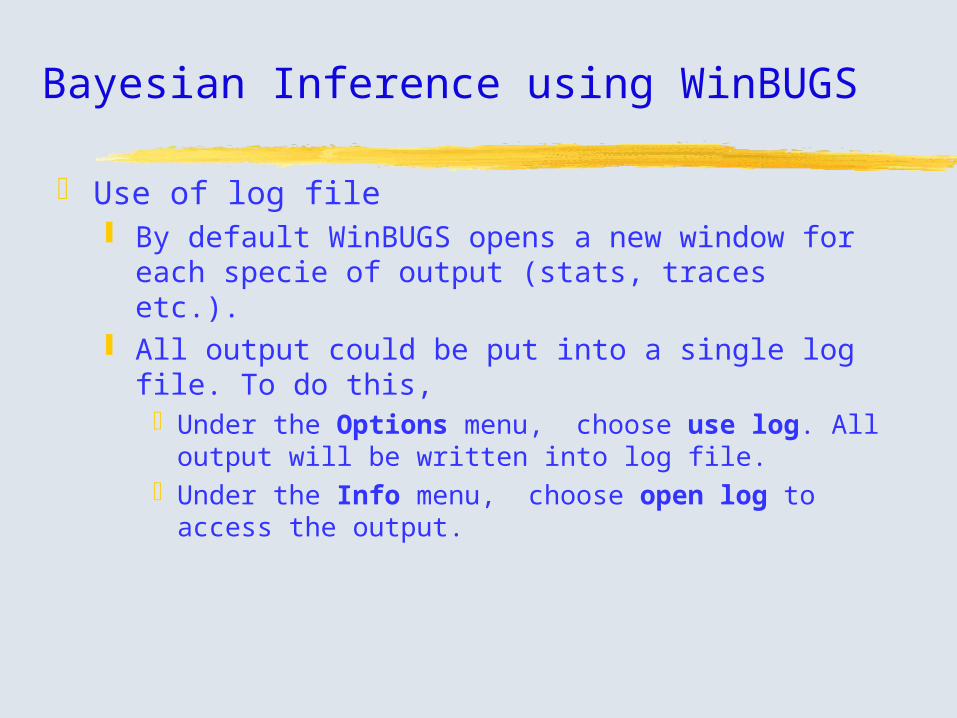
Bayesian Inference using WinBUGS
Use of log file By default WinBUGS opens a new window for each
specie of output (stats, traces etc.). All output could be put into a single log file. To do
this,Under the Options menu, choose use log. All
output will be written into log file. Under the Info menu, choose open log to access
the output.
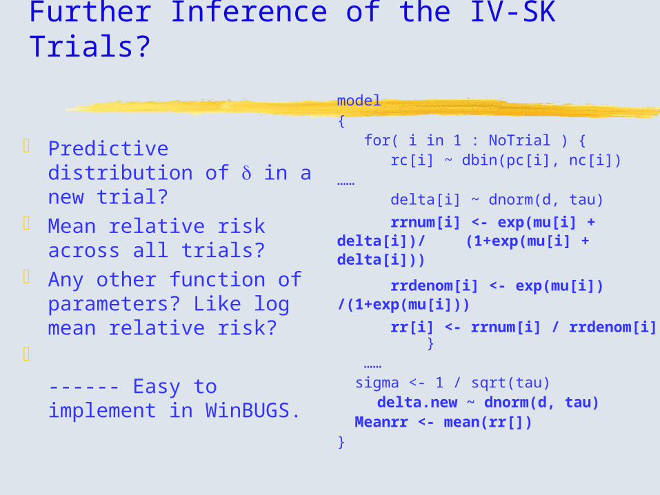
Further Inference of the IV-SK Trials?
Predictive distribution of in a new trial?
Mean relative risk across all trials?
Any other function of parameters? Like log mean relative risk?
------ Easy to implement in WinBUGS.
model{ for( i in 1 : NoTrial ) { rc[i] ~ dbin(pc[i], nc[i])…… delta[i] ~ dnorm(d, tau)
rrnum[i] <- exp(mu[i] + delta[i])/ (1+exp(mu[i] + delta[i]))
rrdenom[i] <- exp(mu[i]) /(1+exp(mu[i]))
rr[i] <- rrnum[i] / rrdenom[i] }
…… sigma <- 1 / sqrt(tau)
delta.new ~ dnorm(d, tau) Meanrr <- mean(rr[])}
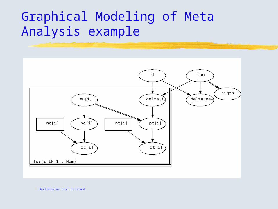
Graphical Modeling of Meta Analysis example
for(i IN 1 : Num)
sigma
taud
delta.newmu[i] delta[i]
pt[i]nt[i]pc[i]nc[i]
rt[i]rc[i]
Rectangular box: constant

Further Inference of the IV-SK Trials
delta.new chains 1:3
iteration10000 20000 30000 40000
-1.5
-1.0
-0.5
0.0
0.5
1.0
History: time series of the samples.
Meanrr chains 1:3
iteration10000 20000 30000 40000
0.6
0.7
0.8
0.9
1.0

Further Inference of the IV-SK Trials
Meanrr chains 3:1
iteration10032 10200 10400 10600
0.7 0.75 0.8 0.85 0.9
delta.new chains 3:1
iteration10032 10200 10400 10600
-1.0 -0.75 -0.5 -0.25 0.0 0.25
Meanrr chains 1:3
lag0 20 40
-1.0 -0.5 0.0 0.5 1.0
delta.new chains 1:3
lag0 20 40
-1.0 -0.5 0.0 0.5 1.0
Meanrr chains 1:3
iteration10000 20000 30000 40000
0.0
0.5
1.0delta.new chains 1:3
iteration10000 20000 30000 40000
0.0
0.5
1.0
Credible sets, autocorrelation (every 50th sample) and convergence diagnostics

Further Inference of the IV-SK Trials
Summary Statistics:
node mean sd MC error 2.5% median 97.5% start sample Meanrr 0.78830.035147.334E-4 0.7207 0.7883 0.8598 10000 2400delta.new -0.2857 0.1482 0.00275 -0.6109 -0.2812 -0.007317 10000
2400
delta.new chains 1:3 sample: 2400
-1.5 -1.0 -0.5 0.0 0.5
0.0
2.0
4.0
6.0Meanrr chains 1:3 sample: 2400
0.6 0.7 0.8 0.9
0.0
5.0
10.0
15.0

Compare with Frequentist results?
Three possibilities of classical approach: the studies are identical replications of each other
Estimate an overall treatment mean from the study The studies are completely unrelated
Estimate one treatment effect for each study. The studies are related to each other
Random effects model --- meta analysisAssume exchangeability but interest often focuses on the
estimate of overall mean. The Bayesian approach:
Uncertainty about the probable effect in a particular population where a study has not been performed might be more represented by inference for a new study effect, exchangeable from those for which studies have been performed, rather than for the over mean.
The effect is predicted by delta.new.

Sensitivity Analysis Sensitivity analysis are often carried out to investigate how much
impact on posterior inference within reasonable modification of priors.
Prior specification Posterior inference
Node Mean 2.5% Median 97.5%
Mu[i] ~ Normal((0.0,1.0E-5)d ~ Normal((0.0,1.0E-6)tau ~ gamma(0.001,0.001)
ddelta.new
sigma
-0.287-0.28430.1165
-0.4161-0.61840.02573
-0.2842-0.27680.09292
-0.1750.046990.3323
Mu[i] ~ Normal((0.0,1.0E-5)d ~ Normal((0.0,1.0E-6)tau ~ gamma(0.1,0.1)
ddelta.new
sigma
-0.3222-0.32440.2932
-0.5131-0.98420.1597
-0.3195-0.31950.2786
-0.14290.33480.4984
Mu[i] ~ Normal((0.0,1.0E-3)d ~ Normal((0.0,1.0E-4)tau ~ gamma(0.001,0.001)
ddelta.new
sigma
-0.2871-0.28580.1178
-0.4232-0.635
0.02386
-0.2814-0.27840.09111
-0.17450.029630.3454
Mu[i] ~ Normal((0.0,1.0E-3)d ~ Normal((0.0,1.0E-4)tau ~ gamma(0.1,0.1)
ddelta.new
sigma
-0.3238-0.31390.2915
-0.5179-0.93970.1581
-0.322-0.31530.2797
-0.14840.30610.4997
Mu[i] ~ Normal((0.0,1.0E-3)d ~ Normal((0.0,1.0E-4)tau ~ gamma(0.01,0.01)
ddelta.new
sigma
-0.2989-0.3016
0.18
-0.4539-0.734
0.06276
-0.2947-0.29350.1611
-0.16540.11630.402

Other features of WinBUGS Under Model menu
Monitor Metropolis: shows minimum, maximum and average acceptance rate of metropolis algorithm.
Save state: shows the current state of all the stochastic variables. Seed: shows and changes the seed of random number generator.
Under Inference menu Fit: looks at model fit, predicted value and residuals of longitudinal data. Correlation: scatter plots and correlation between monitored variables. Summary: mean and standard deviation of variables. Simplified version
of Samples. Ranks: shows the ranks of the simulated values in an array.
Under Info menu Node info: current value, sampling method, type of the node, etc. Components: displays all the components in use.
Doodle menu: graphical representation of the model.
BOA --- Bayesian Output Analysis
Available at: http://www.public-health.uiowa.edu/BOA. Modified version of CODA --- Convergence Diagnostic
and Output Analysis. A set of S-Plus functions which serves as an output
processor for the WinBUGS(BUGS) software. S - plus windows users could open BOA as an script file
and run the file from the script window. Analysis could be done by using
Menu-Driven User Interface Or Command line (shown here).
BOA --- Bayesian Output Analysis
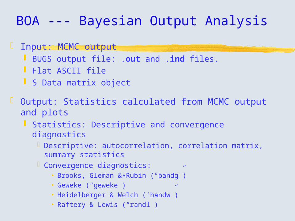
Input: MCMC output BUGS output file: .out and .ind files. Flat ASCII file S Data matrix object
Output: Statistics calculated from MCMC output and plots Statistics: Descriptive and convergence diagnostics
Descriptive: autocorrelation, correlation matrix, summary statistics
Convergence diagnostics:• Brooks, Gleman & Rubin (“bandg”)• Geweke (“geweke”)• Heidelberger & Welch (‘handw”)• Raftery & Lewis (“randl”)

BOA --- Bayesian Output Analysis
Output: Statistics calculated from MCMC output and plots Statistics Plots: Descriptive and convergence diagnostics
Descriptive: autocorrelation, density, running mean and traceConvergence diagnostics: Brooks, Gleman & Rubin ; Geweke ;
Heidelberger & Welch; Raftery & Lewis(“randl”) The descriptive information could be obtained from WinBUGS.
There are options to manage data and change parameter specifications.

BOA: the IV - SK trials------ More convergence diagnostics
To show the diagnostic work of BOA, convergence was check for parameters d and sigma over three chains from the meta - analysis example of the IV - SK trials.
WinBUGS output files: sk1out1: sk1out1.out and sk1out1.ind sk1out2: sk1out2.out and sk1out2.ind sk1out3: sk1out3.out and sk1out3.ind sk1out1.ind, sk1out2.ind, sk1out3.ind are the same index
file produced by CODA in Samples of WinBUGS. Saved three times under three names to facilitate its use in BOA.
Using of BOA through command line Copy boa.s into the script file window and run the file. Start BOA sessions with a call to boa.start().

BOA: the IV - SK trials------ More convergence diagnostics
Sk1_boa.ssc (Appendix D) Start the BOA session.
> boa.start()
Bayesian Output Analysis Program (BOA)
Version 0.99.1 for Windows S-PLUS
Copyright (c) 2001 Brian J. Smith <[email protected]>
………… At this point the global parameters have been assigned default values.
Specify the path where the MCMC output is located.
> boa.par(path = "C:\\Program Files\\WinBUGS13
\\rongwei's files\\",title = "IV-SK Trials")
BOA: the IV - SK trials------ More convergence diagnostics
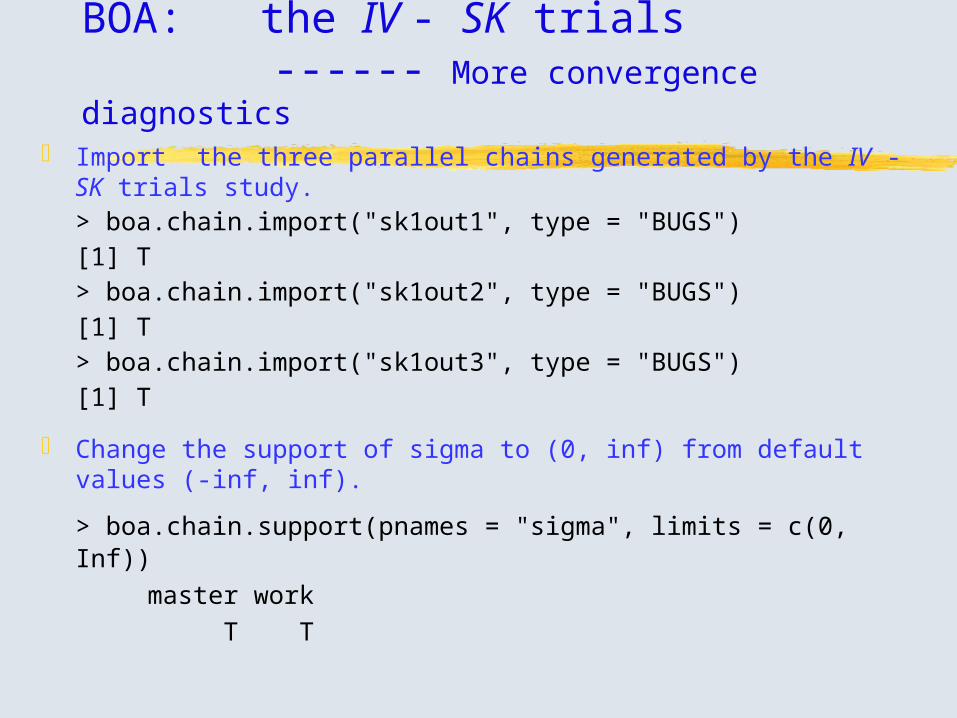
Import the three parallel chains generated by the IV - SK trials study.> boa.chain.import("sk1out1", type = "BUGS")[1] T> boa.chain.import("sk1out2", type = "BUGS")[1] T> boa.chain.import("sk1out3", type = "BUGS")[1] T
Change the support of sigma to (0, inf) from default values (-inf, inf).
> boa.chain.support(pnames = "sigma", limits = c(0, Inf))
master work
T T

BOA: the IV - SK trials------ More convergence diagnostics
Display summary information about the input data --- data check. > boa.print.info()
CHAIN SUMMARY INFORMATION:==========================Iterations:+++++++++++
Min Max Sample sk1out1 1 10000 10000sk1out2 1 10000 10000sk1out3 1 10000 10000
Support: sk1out1----------------
d sigma Min -Inf 0Max Inf Inf
(Cont. from left)
Support: sk1out2----------------
d sigma Min -Inf 0Max Inf Inf
Support: sk1out3----------------
d sigma Min -Inf 0Max Inf Inf

BOA: the IV - SK trials------ More convergence diagnostics
Brooks, Gelman & Rubin Convergence Diagnostic The diagnostic was originally proposed by Gelman and Rubin (1992). Appropriate for the analysis of two or more parallel chains, each with
different starting values which are overdispersed with respect to the target distribution.
Based on a comparison of the within and between chain variance for each variable to estimate the potential scale reduction factor (PSRF) which might be reduced if the chains were run to infinity.
Brooks and Gelman (1998) proposed the corrected scale reduction factor (CSRF) to adjust for the sampling variability in the variance estimates.
Only the second half of the samples is used to compute the reduction factors.
If the estimates are approximately equal to one (or, as a rule of thumb, the 0.975 quantile is < 1.2), the samples may be considered to have arisen from the stationary distribution.

BOA: the IV - SK trials------ More convergence diagnostics
Brooks, Gelman & Rubin Convergence Diagnostic Estimate of PSRF --- very close to 1 and 97.5% quantile < 1.2.
> boa.print.gandr()BROOKS, GELMAN AND RUBIN CONVERGENCE DIAGNOSTICS:===============================================Iterations used = 5001:10000
Potential Scale Reduction Factors--------------------------------- d sigma 1.005053 1.001255Multivariate Potential Scale Reduction Factor = 1.0048224Corrected Scale Reduction Factors--------------------------------- Estimate 0.975 d 1.006186 1.019995sigma 1.002439 1.006100

BOA: the IV - SK trials------ More convergence diagnostics
Brooks, Gelman & Rubin Convergence Diagnostic plots of CSRF
> boa.plot("gandr")
[1] T
Last Iteration in Segment
Sh
rin
k F
acto
r
0 2000 4000 6000 8000 10000
1.0
01
.04
1.0
8 d0.975Median
Gelman & Rubin Shrink Factors
IV-SK Trials
Last Iteration in Segment
Sh
rin
k F
acto
r
0 2000 4000 6000 8000 10000
1.0
1.2
1.4
1.6
sigma0.975Median
Gelman & Rubin Shrink Factors
IV-SK Trials
BOA: the IV - SK trials------ More convergence diagnostics
Geweke convergence diagnostic The diagnostic was proposed by Geweke (1992). Appropriate for the analysis of individual chains when
convergence of the mean of some function of the sampled parameters is of interest.
The chain is divided into two "windows" containing a set fraction of the first and the last iterations.
A Z statistic was calculated to compare the means of the two “windows”.
As the number of iterations approaches infinity, the Z statistic approaches the N(0,1) if the chain has converged.
There is evidence against convergence when the p-value is less than 0.05. Otherwise, the test does not provide any evidence against convergence. This does not, however, prove that the chain has converged.

BOA: the IV - SK trials------ More convergence diagnostics
Geweke Convergence Diagnostic Estimate of Z - statistic --- against convergence of mean
> boa.print.geweke()
GEWEKE CONVERGENCE DIAGNOSTIC:
=============================
Fraction in first window = 0.1
Fraction in last window = 0.5
Chain: sk1out1
--------------
d sigma
Z-Score -3.5375257704 4.26733872093
p-value 0.0004038948 0.00001978187

BOA: the IV - SK trials------ More convergence diagnostics
Geweke Convergence Diagnostic Estimate of Z - statistic --- against convergence, more runs?
> boa.print.geweke() (cont.)
GEWEKE CONVERGENCE DIAGNOSTIC:=============================Chain: sk1out2-------------- d sigma Z-Score -1.73801549 3.9334628119p-value 0.08220808 0.0000837308
Chain: sk1out3-------------- d sigma Z-Score 0.7641664 -3.5127337258p-value 0.4447681 0.0004435217
BOA: the IV - SK trials------ More convergence diagnostics
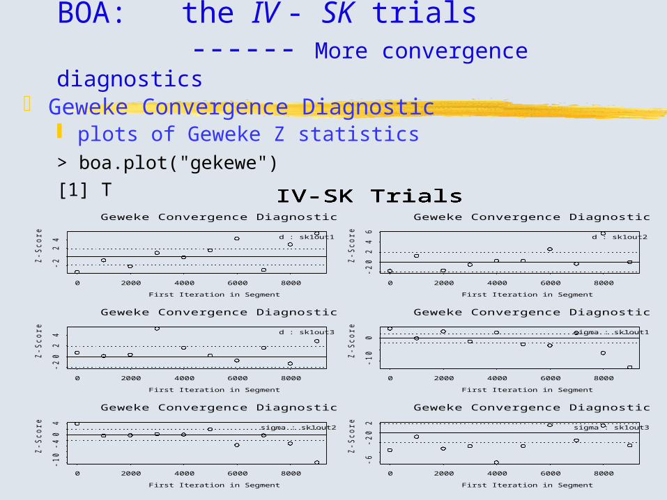
Geweke Convergence Diagnostic plots of Geweke Z statistics> boa.plot("gekewe")
[1] T
First Iteration in Segment
Z-S
co
re
0 2000 4000 6000 8000
-22
4 d : sk1out1
Geweke Convergence Diagnostic
IV-SK Trials
First Iteration in Segment
Z-S
co
re
0 2000 4000 6000 8000
-20
24
6
d : sk1out2
Geweke Convergence Diagnostic
IV-SK Trials
First Iteration in Segment
Z-S
co
re
0 2000 4000 6000 8000
-20
24 d : sk1out3
Geweke Convergence Diagnostic
IV-SK Trials
First Iteration in Segment
Z-S
co
re
0 2000 4000 6000 8000
-10
0
sigma : sk1out1
Geweke Convergence Diagnostic
IV-SK Trials
First Iteration in Segment
Z-S
co
re
0 2000 4000 6000 8000
-10
-40
4
sigma : sk1out2
Geweke Convergence Diagnostic
IV-SK Trials
First Iteration in Segment
Z-S
co
re
0 2000 4000 6000 8000
-6-2
02
sigma : sk1out3
Geweke Convergence Diagnostic
IV-SK Trials

BOA: the IV - SK trials------ More convergence diagnostics
Heidelberger and Welch convergence diagnostic The diagnostic was proposed by Heidelberger and Welch
(1983). Appropriate for the analysis of individual chains.
Based on Brownian bridge theory and uses the Cramer-von-Mises statistic.
If there is evidence of non-stationarity, the test is repeated after discarding the first 10% of the iterations and continues until the resulting chain passes the test or more than 50% of the iterations have been discarded.
BOA reports the number of iterations that were kept, the number of iterations that were discarded, and the Cramer-von-Mises statistic. Failure of the chain to pass this test indicates that a longer run of the MCMC sampler is needed in order to achieve convergence.

BOA: the IV - SK trials------ More convergence diagnostics
Heidelberger and Welch convergence diagnostic (cont.) A halfwidth test is performed on the portion of the chain
that passes the stationarity test for each variable.
Spectral density estimation is used to compute the asymptotic standard error of the mean.
If the half-width of the confidence interval for the mean is less than a specified fraction (accuracy) of this mean, the halfwidth test indicates that the mean is estimated with acceptable accuracy.
Failure of the halfwidth test implies that a longer run of the MCMC sampler is needed to increase the accuracy of the estimated posterior mean.

BOA: the IV - SK trials------ More convergence diagnostics
Heidelberger and Welch Convergence Diagnostic Estimate of diagnostic statistics
> boa.print.handw()
HEIDLEBERGER AND WELCH STATIONARITY AND INTERVAL HALFWIDTH TESTS:
===================================================
Halfwidth test accuracy = 0.1
Chain: sk1out1--------------
Stationarity Test Keep Discard C-von-M d passed 9000 1000 0.2703470sigma passed 7000 3000 0.3615584
Halfwidth Test Mean Halfwidth d passed -0.2853485 0.004450549sigma passed 0.1171427 0.007776577

BOA: the IV - SK trials------ More convergence diagnostics
Heidelberger and Welch Convergence Diagnostic Estimate of diagnostic statistics
> boa.print.handw()(cont.)
Chain: sk1out2--------------
Stationarity Test Keep Discard C-von-M d passed 10000 0 0.07425641sigma passed 10000 0 0.34860040
Halfwidth Test Mean Halfwidth d passed -0.2876464 0.004084248sigma passed 0.1211367 0.007508664

BOA: the IV - SK trials------ More convergence diagnostics
Heidelberger and Welch Convergence Diagnostic Estimate of diagnostic statistics
> boa.print.handw()(cont.)
Chain: sk1out3--------------
Stationarity Test Keep Discard C-von-M d passed 10000 0 0.4266263sigma passed 5000 5000 0.1765119
Halfwidth Test Mean Halfwidth d passed -0.2878423 0.004138602sigma passed 0.1247507 0.010573640

BOA: the IV - SK trials------ More convergence diagnostics
Raftery and Lewis convergence diagnostic was proposed by Raftery and Lewis (1992b). Appropriate for the analysis of individual chains. The diagnostic tests for convergence to the stationary
distribution and estimates the run-lengths needed to accurately estimate quantiles of functions of the parameters.
BOA computes the "lower bound" - the number of iterations needed to estimate the specified quantile to the desired accuracy using independent samples.
If sufficient MCMC iterations are available, BOA lists the lower bound, the total number of iterations needed for each parameter, the number of initial iterations to discard as the burn-in set, and the thinning interval to be used.
The dependence factor measures the multiplicative increase in the number of iterations needed to reach convergence due to within-chain correlation.
Dependence factors greater than 5.0 often indicate convergence failure and a need to reparameterize the model (Raftery and Lewis, 1992a).

BOA: the IV - SK trials------ More convergence diagnostics
Raftery and Lewis Convergence Diagnostic Estimate of dependence factor --- against convergence
> boa.print.randl()
RAFTERY AND LEWIS CONVERGENCE DIAGNOSTIC:
=========================================
Quantile = 0.025
Accuracy = +/- 0.005
Probability = 0.95
Chain: sk1out1
--------------
Thin Burn-in Total Lower Bound Dependence Factor
d 7 21 32781 3746 8.750934
sigma 7 28 27083 3746 7.229845

BOA: the IV - SK trials------ More convergence diagnostics
Raftery and Lewis Convergence Diagnostic Estimate of dependence factor --- against convergence
> boa.print.randl()(cont.)
Chain: sk1out2
--------------
Thin Burn-in Total Lower Bound Dependence Factor
d 6 18 24816 3746 6.624666
sigma 9 36 42363 3746 11.308863
Chain: sk1out3
--------------
Thin Burn-in Total Lower Bound Dependence Factor
d 8 40 50600 3746 13.507742
sigma 10 30 28020 3746 7.479979

More BUGS Sources Website of BUGS: for all information
http://www.mrc-bsu.cam.ac.uk/bugs/winbugs/contents.shtml Two add add-ons:
PKBUGSComplex population pharmacokinetic/pharmacodynamic
(PK/PD) modeling http://www.med.ic.ac.uk/divisions/60/pkbugs_web/home.html
GeoBUGSa demonstrator version for epidemiological mapping studiesfits spatial models and produces a range of maps as output.http://www.mrc-bsu.cam.ac.uk/bugs/winbugs/geobugs.shtml
BUGS on the web Features examples of BUGS or WinBUGS in different disciplines. http://www.mrc-bsu.cam.ac.uk/bugs/weblinks/
webresource.shtml

Last reminder
I am the BUGS!
Hoped I had entertained you!Last reminder: Beware - MCMC sampling
can be dangerous in WinBUGS!
Selected Reference
Brooks, S.P. and Gelman A. 1998. General methods for monitoring convergence of iterative simulations. J. Comp. Graph. Statist. 7., 434-455.
Gelman, A. and Rubin, D. B. (1992). Inference from iterative simulation using multiple sequences. Statistical Science, 7, 457-72.
Gilks, W. R. (1992). Derivative-free adaptive rejection sampling for gibbs sampling. In Bayesian Statistics 4, (ed. J. M. Bernardo, J. O. Berger, A. P. Dawid, and A. F. M. Smith), pp. 169-94. Clarendon Press, Oxford, UK.
Geweke, J. (1992). Evaluating the accuracy of sampling-based approaches to calcualting posterior moments. In Bayesian Statistics 4, (ed. J. M. Bernardo, J. O. Berger, A. P. Dawid, and A. F. M. Smith). Clarendon Press, Oxford, UK.
Heidelberger, P. and Welch, P.D. 1983. Simulation run length control in the presence of an initial transient . Operations Research, 31, 1109-1144.
Neal, R.M. (1997). Markov chain Monte Carlo methods based on ‘slicing’ the density function. Technical Report No. 9722, Dept of Statistics, University of Toronto.
Raftery, A.E. and Lewis, S. 1992a? How many iterations is the Gibbs sampler? In Bayesian Statistics 4, J.M . Bernardo, J. O. Berger, A. P. Dawid, and A.F. M. Smith, eds., Oxford: Oxford University Press, pp.763-773.