An inverse modelling technique for glass

forming by gravity sagging

Y. Agnon a Y.M. Stokes b,∗

aDepartment of Civil and Environmental Engineering, Technion, Israel Institute of

Technology, 32000 Haifa, Israel.

bApplied Mathematics, School of Mathematical Sciences, University of Adelaide,

5005 Australia.

Abstract

Some optical surfaces are formed by gravity sagging of molten glass. A glass sheetsupported on a ceramic former is heated; the glass becomes a very viscous fluid andsags under its own weight until the lower surface is in full contact with the former.The smooth upper free surface is the required optical surface. Its shape is dependenton the initial geometry and, in optical terms, differs significantly from the formershape. The inverse problem is to determine the shape of the former that producesa prescribed upper surface. This is a difficult, highly nonlinear problem. A finiteelement algorithm has been developed to compute gravity sagging for any giveninitial geometry (the forward problem). The present work describes a successfuliterative method, which uses the output from a number of forward problems todetermine the required former shape.

Key words: Inverse problem, creeping flow, free surface, glass forming

1 Introduction

Thermal replication is a process used in the production of aspheric opticalcomponents as described in [9,12] and shown in Figure 1. A glass workpiece orpre-form is placed on a ceramic former which has been previously machined toa given shape. This combination is heated in an oven so that the glass meltsand sags, or ‘slumps’, under its own weight into the former. On cooling theglass component is removed from the former. Its lower surface is rough due to

∗ Corresponding author. Tel.: +61-8-8303-4808; fax: +61-8-8303-3696.Email address: ystokes@maths.adelaide.edu.au (Y.M. Stokes).

Preprint submitted to Elsevier Science 26 May 2004

z = F (r, θ)6

¤¤¤²R0

-a (= 1)

- r

6z

s

?6d?6h

ceramic former

glass workpiece

(a) Before slumping; with geometrical

notation.

ceramic former

mould

progressive surface M(r, θ)¢¢®

(b) After slumping; top surface has

curvature profile M(r, θ).

Fig. 1. The thermal replication process.

contact with the rough former, but the upper surface is smooth and may beused, for example, as a mirror surface or as a mould surface for casting plasticophthalmic lenses; the curvature of this surface must meet the design criteriato sufficient optical precision. The process takes its name from the idea of‘replicating’ the basic shape of the ceramic former on the upper glass surfacewhile smoothing out any small scale imperfections in the former surface arisingfrom machining. However, the transfer of even the basic former shape to theglass is not exact, especially in terms of surface curvature which is the quantityof primary interest for optical components.

This is an example of a highly nonlinear inverse problem. The process designermust determine the geometry of the former and pre-form and the temperature-time profile to yield the required product; the product designer must ensurethat the product is achievable by thermal replication. Solving this inverseproblem is much more difficult than solving the forward problem of determin-ing the product yielded by a given geometrical setup and temperature-timehistory.

Such inverse problems are important in industrial forming processes. Theyarise, for example, in the manufacture of automotive windscreens [3,5], inthermoforming of plastics [1,2,14,20] and in forging [7,13,21], to name a fewwhich appear in the literature. For these examples temperature is an impor-tant control on the product being produced and much of the literature isconcerned with inverse methods for determining suitable temperature profilesin space and time [1,2,5,11,20]. In relation to geometrical controls, work onshape optimisation of an initial workpiece or preform includes [13,14] while[7,21] consider the optimisation of die shape design to minimise forming loadand achieve deformation uniformity respectively. This paper presents a methodfor determining mould (or former) shapes to yield a desired product shape.While we specifically focus on thermal replication of optical components, themethod described has more general applicability.

It is generally accepted that molten glass may be modelled as a very viscousNewtonian fluid [10]; non-Newtonian behaviour is important in only relatively

2

few situations (see, for example, [6]). In the problem of present interest the flowis very slow with a time scale of hours. Working temperatures are around 700◦Cwith glass viscosity µ of the order of 106 Pa.s. Slumping velocities scale likeρga2/µ, where ρ ∼ 2500 kg/m3, g and a are density, gravitational accelerationand a typical length scale, respectively. Here the length scale a is the pre-formradius, about 45 mm. Then, the Reynolds number ρ2ga3/µ2 ∼ 6×10−6 is verysmall and, as in many other glass-forming processes [4,8,18,19], we are justifiedin neglecting the inertial terms in the Navier-Stokes equation and solving theNewtonian creeping-flow (or Stokes flow) equations

−∇p + ∇ · (µ∇u) − ρg k = 0

together with the continuity equation

∇ · u = 0,

where p and u are pressure and velocity respectively, and k is the unit vectorpointing vertically up.

We are also justified in neglecting surface tension, since the Capillary numberis large, scaling as ρga2/σ, where σ ≈ 0.3 N/m is the coefficient of surfacetension for glass. Thus we must solve the creeping-flow equations subject tono-slip conditions (u = 0) where the molten glass is in contact with a solidboundary, and zero-stress and kinematic conditions on the free-surface bound-aries elsewhere.

Thermal replication clearly involves heat flow in addition to fluid flow. How-ever, the glass-former combination is heated in a closed oven in which spatialtemperature variations over distances comparable to the pre-form diameterare small, so that we may assume that the temperature, and hence the vis-cosity µ, in the glass is a function of time t only. Further, as explained in [17]a consequence of using a creeping-flow model is that temporal changes in theviscosity affect only the slump time, but not the final product. Then, we mayeffectively account for a time-varying viscosity within the time scale and, fora given constant value of the dimensionless slump time

T = ρg∫ 1

µ(t)dt,

the shape of the optical surface resulting from a given initial geometrical setupis determined by solving for the flow of the molten glass assuming a constantviscosity, such that T = ρgt/µ; there is no need to solve a coupled heat andfluid flow problem.

Solution of the forward problem of determining the top surface shape of theglass for a given (axisymmetric) former shape and initial pre-form geometry isdiscussed in detail in [15–17] and we give just a brief summary of the methods

3

used here. The Newtonian creeping-flow equations are solved in the glass,subject to no-slip where the glass is in contact with the former and zero-stressconditions on free surfaces, using a finite-element method. Lagrangian time-stepping is used to track the changing geometry of the glass over time. Atthe end of the process, when the lower surface of the glass workpiece is in fullcontact with the ceramic former, the curvature profile of the upper surface iscomputed using a least-squares quintic B-spline fit to surface coordinate data.We assume here that the forward problem is solved satisfactorily in this way.

We are, therefore, left with the inverse problem: to determine the geometricalsetup to give the required optical surface. Both the former and preform shapesinfluence the final outcome, but the former shape is by far the most impor-tant control and adjusting its shape the best mechanism for modifying theoptical surface. Our primary focus is therefore on determining former shape.At present this is done by a time-consuming, iterative experimental procedureand we here propose a computational approach which can be used to investi-gate the range of surface profiles that can be made by thermal replication andwhich may be developed into a tool that can replace experiments and reduceprocess design time.

2 Notation

We consider a glass disc pre-form of radius a, thickness h and initial radius ofcurvature R0, and a former of radius a, with cavity surface described in termsof elevation z = F (r, θ) such that there is a maximum distance d between theformer and the lower pre-form surface, as shown in Figure 1. We shall workin cylindrical polar coordinates (r, θ, z) where z = 0 is the plane of support ofthe glass. Next, we non-dimensionalise using a as the length scale, equivalentto setting a = 1. Then h becomes the aspect ratio of the pre-form and dthe aspect ratio of the former cavity. The desired curvature profile on the topsurface of the glass is K(r, θ), while the actual curvature profile after slumpingis M(r, θ).

We here restrict our attention to axisymmetric geometries, although we usenotation applicable to general three-dimensional problems to which our meth-ods are, in principle, readily extended. Then we may use the symmetry of theproblem and restrict our computational domain to one radius of the geometry.Information supplied by the industry indicates that the glass thickness is suchthat 0.04 ≤ h ≤ 0.15 covers the full range of possibilities for the pre-form as-pect ratio, while 0.01 ≤ d ≤ 0.10 is a suitable parameter range for the aspectratio of the former cavity; R0, the initial curvature of the pre-form, is chosenso that d does not exceed this range. Typically h = 0.1333 and d = 0.0444.Unless otherwise stated, we use R0 = ∞ corresponding to a flat pre-form.

4

3 A zeroth-order solution

A zeroth-order estimate of the transfer function from former to glass is ob-tained assuming that, at the end of the slumping process, the glass forms alayer of uniform thickness h over the former surface F (r, θ). Such a simpleshift function is not sufficiently accurate for optical products where the cur-vature is important. Rather, the transfer function is a complex function thathas nonlinear dependence on geometrical parameters, such as the depth of themould and the thickness of the pre-form.

The solution method we will describe is based on approximate linear super-position, starting from an initial estimate of the solution such as provided bythe zeroth-order solution and, hence, we begin by looking more closely at thissolution. We note that curvature is itself a nonlinear function (z′′/(1+z′2)3/2,where z is surface elevation and primes denote differentiation with respectto r) and, strictly, cannot be obtained by superposition. However, the slopeof the surfaces considered are small, so that the curvature is almost identi-cal with the second derivative of the surface which can be obtained by linearsuperposition. Hence we will use the second derivative everywhere in placeof curvature, while retaining the name “curvature”, although we could alsouse the curvature function itself since the error introduced is small relative toother components of the error.

Suppose that we wish to obtain a constant curvature on the glass by slump-ing into a spherically shaped former. Then, to zeroth-order we expect thecurvature of the top glass surface to be constant at K = 1/(Rf − h), whereRf = (1 + d2)/(2d) is the radius of curvature of the former. Let K be the de-sired curvature profile. The error E(r, θ) is the difference between the actualsurface curvature M and the desired curvature, i.e. E = M − K, and |E| isconstrained by some industry-prescribed tolerance function. Usually, the tol-erance is smaller at the centre and increases towards the edge. Since the glassis edge trimmed after slumping, we need only be concerned with E over somerange 0 ≤ r < b, b < a, although to minimise waste it is desirable that b beas close to the glass and former radius a as possible.

Noting that both d and h are typically small, we may write

K =2d

1 + d2 − 2dh≈ 2d, (1)

from which we might expect the actual curvature profile M to be, not onlynear constant, but also reasonably linearly dependent on the aspect ratio ofthe former cavity d and independent of h. Thus we might expect there to bea function f(r) ≈ 2 such that M(r)/d ≈ f(r).

5

Figure 2 shows the scaled curvature profile M(r)/d for different values ofd ∈ [0.01, 0.10] and for a flat pre-form of fixed aspect ratio h = 0.1333; thesolution of the forward problem was taken when full contact of the lower glasssurface with the mould had been attained, which occurs at different times forthe different formers. We see that, in the central region r < 0.1 and near theedge r > 0.6, M/d varies from two by an amount greater than can be accountedfor by the approximation (1). Also, we note that M/d reduces to almost thesame curve in the central region of the disc, showing that M increases almostlinearly with d in this region for each of the four cases considered. However,elsewhere M depends on d in a more nonlinear manner.

Figure 3 shows the effect of the pre-form aspect ratio on the scaled curvatureM/d for slumping into a former with cavity aspect ratio d = 0.05; for thisfigure the solution to the forward problem was taken at the same time foreach of the cases considered and when there was full contact of the lowerglass surface with the former. Clearly, the deviation of M from (1) is quitedependent on h and the smaller h the better is the approximation M/d = 2.For the thinnest glass h = 0.05, the top surface curvature profile is noticeablyless smooth than the curves for the thicker pre-forms. We believe this to be dueto mould roughness (due to a piecewise linear mould representation) and/orroughness resulting from contact events between the glass and former, whichis not sufficiently smoothed out when the glass is thin.

It is evident that the inaccuracy of the zeroth-order method for determiningthe former profile F to yield a desired curvature profile K on the glass increaseswith both the cavity aspect ratio of the former d and the aspect ratio of the pre-form h. Not unexpectedly, thinner glass more accurately replicates the formercurvature; but defects in the former surface are more likely to be transferred tothe glass also. Since a sufficiently thick glass pre-form must be used to dampout small-scale imperfections in the former, our task is to devise a methodfor modifying the former profile to reduce the curvature error E, given thepre-form aspect ratio h.

4 Former modification: linearised approach

The idea used is essentially that of the multivariable Newton-Raphson method.Our zeroth-order method gives an estimate of the former elevation profilez = F (r, θ) for a given desired curvature K(r, θ) on the top surface of theglass. On slumping we find that the actual curvature profile is M(r, θ). Wedenote this

F (r, θ) ⇒ M(r, θ).

6

1.9

1.95

2

2.05

2.1

2.15

2.2

2.25

2.3

0 0.2 0.4 0.6 0.8 1

M/d

r

d = 0.0250.0500.0750.100

Fig. 2. M/d for a glass pre-form of aspect ratio h = 0.1333 slumping into sphericalformers of different cavity aspect ratio d. The curves were computed after full mouldcontact at times t = 0.075, 0.100, 0.125, 0.150 for d = 0.025, 0.050, 0.075, 0.100respectively.

1.9

1.95

2

2.05

2.1

2.15

2.2

2.25

2.3

0 0.2 0.4 0.6 0.8 1

M/d

r

h = 0.050.10

0.13330.15

Fig. 3. M/d for glass pre-forms of different aspect ratio h slumping into a sphericalformer with cavity aspect ratio d = 0.05. The curves were all computed at timet = 0.100 by which time full mould contact had been established in each case.

If M is sufficiently close to K then

K(r, θ) = M(r, θ) + δM(r, θ),

where δM is a small perturbation of M , and we need to find a small pertur-bation δF of F such that

F (r, θ) + δF (r, θ) ⇒ M(r, θ) + δM(r, θ).

We define δM to be the target and δF to be the solution. Now, we maysolve the forward problem for each of a ‘basis’ set of m former perturbationsδi(r, θ), i = 1,m, and determine the corresponding glass surface perturbations

7

µi(r, θ), i = 1,m, i.e.

F (r, θ) + δi(r, θ) ⇒ M(r, θ) + µi(r, θ).

Then, assuming a (nearly) linear response we have

F (r, θ) +m∑

i=1

αiδi(r, θ) ⇒ M(r, θ) +m∑

i=1

αiµi(r, θ),

and we need only determine the coefficients αi such that

δM(r, θ) ≈m∑

i=1

αiµi(r, θ).

These are found by taking J ≥ m collocation points rj, j = 1, J , in the regionof interest (0 ≤ r ≤ b), and determining the best-least-squares solution to theresulting J × m system of equations. The solution is then given by

δF (r, θ) =m∑

i=1

αiδi(r, θ),

and the new former shape is F = F + δF . Setting F = F we may repeat thisprocedure, iterating until M is sufficiently close to K, i.e. |E| = | − δM | issufficiently small over 0 ≤ r ≤ b, or until we are unable to reduce the errorany further.

Now, we may think of the former perturbation as being comprised of a (pos-sibly infinite) linear combination of Fourier components, i.e. δF =

∑i αiδi

with each of the δi contributing a component of a different wavenumber. Asmall wavenumber (long wavelength) former perturbation δi is expected toproduce an essentially small wavenumber perturbation µi on the glass, so thatthe target δM can be similarly considered as a Fourier series. Assuming thatthe target is a well-behaved function, small wavenumber components will beof larger amplitude and more linear than larger wavenumber components andshould be determined first and removed from the target to give a new targetcomprised of the larger wavenumber components. Hence, we adopt an itera-tive approach. We first rank the δi from smallest to largest wavenumber. Thenat iteration m we use the above described procedure with the set of formerperturbations δi, i = 1,m. From the solution δF obtained we obtain a newformer and a new target to be used at iteration m + 1. This new target is,essentially, comprised of Fourier components µi, i > m of larger wavenumberthan already considered, having a solution comprised of Fourier componentsδi, i > m. The physics of slumping, which is designed to smooth out smallscale perturbations on the former, also supports this iterative approach andindicates that there will be a limit on the size and amplitude of perturbationthat can be used effectively.

8

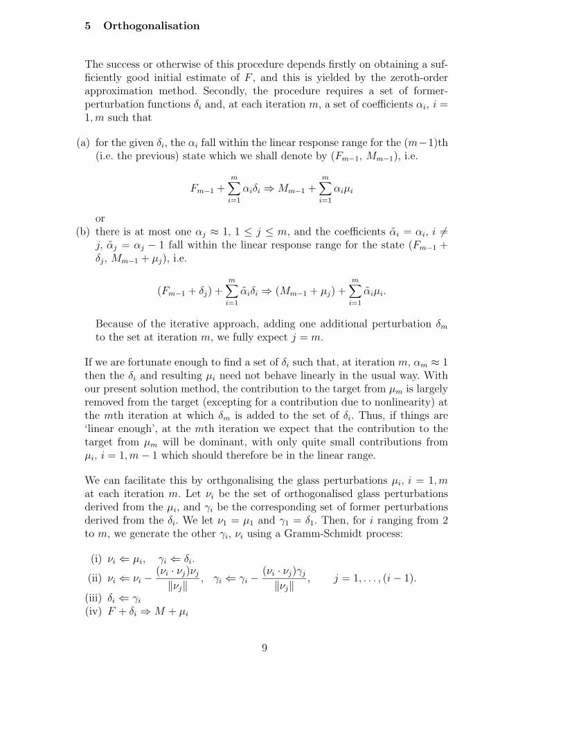
5 Orthogonalisation

The success or otherwise of this procedure depends firstly on obtaining a suf-ficiently good initial estimate of F , and this is yielded by the zeroth-orderapproximation method. Secondly, the procedure requires a set of former-perturbation functions δi and, at each iteration m, a set of coefficients αi, i =1,m such that

(a) for the given δi, the αi fall within the linear response range for the (m−1)th(i.e. the previous) state which we shall denote by (Fm−1, Mm−1), i.e.

Fm−1 +m∑

i=1

αiδi ⇒ Mm−1 +m∑

i=1

αiµi

or(b) there is at most one αj ≈ 1, 1 ≤ j ≤ m, and the coefficients αi = αi, i 6=

j, αj = αj − 1 fall within the linear response range for the state (Fm−1 +δj, Mm−1 + µj), i.e.

(Fm−1 + δj) +m∑

i=1

αiδi ⇒ (Mm−1 + µj) +m∑

i=1

αiµi.

Because of the iterative approach, adding one additional perturbation δm

to the set at iteration m, we fully expect j = m.

If we are fortunate enough to find a set of δi such that, at iteration m, αm ≈ 1then the δi and resulting µi need not behave linearly in the usual way. Withour present solution method, the contribution to the target from µm is largelyremoved from the target (excepting for a contribution due to nonlinearity) atthe mth iteration at which δm is added to the set of δi. Thus, if things are‘linear enough’, at the mth iteration we expect that the contribution to thetarget from µm will be dominant, with only quite small contributions fromµi, i = 1,m − 1 which should therefore be in the linear range.

We can facilitate this by orthgonalising the glass perturbations µi, i = 1,mat each iteration m. Let νi be the set of orthogonalised glass perturbationsderived from the µi, and γi be the corresponding set of former perturbationsderived from the δi. We let ν1 = µ1 and γ1 = δ1. Then, for i ranging from 2to m, we generate the other γi, νi using a Gramm-Schmidt process:

(i) νi ⇐ µi, γi ⇐ δi.

(ii) νi ⇐ νi −(νi · νj)νj

‖νj‖, γi ⇐ γi −

(νi · νj)γj

‖νj‖, j = 1, . . . , (i − 1).

(iii) δi ⇐ γi

(iv) F + δi ⇒ M + µi

9

Note that having obtained new former perturbations δi at (iii) we must slumpagain using these at (iv) to find the corresponding glass perturbations µi, whichare therefore not exactly orthogonal. We may iterate to improve orthogonality,the trade-off being the large amount of computing time that this involves.However, we can check orthogonality as we proceed and perform only as manyiterations as necessary. For the cases considered herein, one to three were used.

Our final algorithm incorporating all of the features discussed to date is givenin Appendix A.

6 Linearity of response

Since the effectiveness of our solution method depends on the validity of ourlinearity assumptions, we next explore the issue of linearity.

For this we consider a pre-form of aspect ratio h = 0.1333 slumping into aformer which has cavity surface elevation z = F +δi, where z = F (r, θ) definesa spherical cavity surface with cavity aspect ratio d = 0.05 and δi is a smallperturbation of this surface. Let us consider the set of small perturbations

δi =ǫ

2(1 + (−1)i+1 cos(iπr)), i = 1, 2, . . . , (2)

where ǫ is a small number determining the amplitude of the perturbation andi = 2/λ is the number of wavelengths of length λ across the diameter of theformer, i.e. k = iπ = 2π/λ is the wavenumber. The functions δi have theproperty of zero perturbation of the former at its edge r = 1, which is takenas a fixed reference. Then linearity of the response demands that

F + (αδi + βδj) ⇒ M + µi,α;j,β,

where

µi,α;j,β = µi,α + µj,β = αµi + βµj,

after a fixed slump time, which we take to be a little more than the time forthe glass to achieve full contact with the unperturbed former.

We first consider multiplicative linearity by setting β = 0 and, for values ofi and ǫ, compute the response µi,α for perturbations αδi for various values α.Linearity demands that µi,α = αµi and hence can be measured by computingeN = µi,α − αµi. Then for a given i we need to determine a value of ǫ and therange of values of α such that |eN | is small. Because the glass is edge trimmed,we are not concerned too much with nonlinearity near the edge and may focusattention on the inner region. In fact these linearity computations will givean indication of the amount of edge trim required. We shall notionally allow

10

-0.005

-0.004

-0.003

-0.002

-0.001

0

0.001

0.002

0.003

0.004

0.005

0 0.2 0.4 0.6 0.8 1

µi

r

i = 125

Fig. 4. Slumping of a pre-form of aspect ratio h = 0.1333 into a base spherical mouldwith d = 0.05 at t = 0.1. Response µi to former perturbations δi with ǫ = 0.001/i2

for i = 1, 2, 5.

-0.003

-0.0025

-0.002

-0.0015

-0.001

-0.0005

0

0.0005

0.001

0.0015

0.002

0 0.2 0.4 0.6 0.8 1

e N

r

Fig. 5. Slumping of a pre-form of aspect ratio h = 0.1333 into a base spheri-cal mould with d = 0.05 at t = 0.1. Error eN = µi,α − αµi for i = 1, 2, 5 andα = ±1,±6,±7, . . . ,±10.

|eN | ∼ 0.001, based on very approximate information from the industry andnoting that the permissible tolerance varies greatly with position on the lensmould. For this reason and because of the iterative nature of our method,this is not a rigid tolerance and more nonlinearity may be permissible in someareas and/or a tighter tolerance in others.

After some experimenting, we have found ǫ = 0.001 i−2 to be a suitable scalingfor δi. The i−2 factor is not too surprising, since it cancels the i2 factor in theformer curvature perturbation function δ′′i = (iπ)2(−1)i+2(ǫ/2) cos(iπr) andhence keeps the magnitude of the former curvature perturbation (and hencethat of the glass curvature) from growing with the wavenumber of the pertur-bation. Figure 4 shows the curvature perturbations µi resulting from formerperturbations δi, i = 1, 2, 5, and Figure 5 shows the error due to nonlinearity

11

eN for αδi, i = 1, 2, 5, and values of α in the range −10 ≤ α ≤ 10. These re-sults were obtained after a slump time of t = 0.1 when there was full contactbetween the glass and former. Note that full contact is important; linearity isconsiderably worse where this is not achieved. The largest error at the centre(|eN | ∼ 0.1) corresponds to the case i = 2, α = 10, and the sudden increasein error in the central region signals that we are entering a highly nonlinearzone. For other perturbations the error is very small at the centre and growstowards the edge. The increased error around r ∼ 0.8 and beyond is an effectof the physical former edge.

Outside of the ‘linear’ response range, eN depends in a complex manner onboth the wavelength and amplitude of the perturbation, due to the differingways in which the glass contacts the former. Excluding the error curve fori = 2, α = 10, the results shown in Figures 4 and 5 are for a glass componentthat first contacts the former at the centre and then progressively from thecentre up and the edge down. However, depending on the location and sizeof humps and holes in the former, initial contact may occur at some otherposition, significantly slowing the sag rate and resulting in different sequencesof contact events, often with the result that full contact between glass andformer is not achieved in the slump time. This, in turn, results in significantlydifferent curvature profiles on the glass and much nonlinearity. The case i =2, α = 10, shown in Figure 5, is an example of such a change in the sequenceof contact events, leading to a change in the nature of the error curve. To keepclose to linear, the perturbation functions should be such that initial contactis at the centre of the former and the glass fully contacts the former in theslump time.

Next we consider perturbations αδi+βδj, i 6= j for which linearity is measuredby eN = µi,α;j,β − αµi − βµj. Curvature perturbations for i = 1, j = 2 andα = ±1, β = ±1 are given in Figure 6 and show a fair degree of symmetry,which is interesting. Plots for i, j = 1, 5 and i, j = 2, 5 show similar symmetryand curvature perturbations of a similar order of magnitude, although thecurves, of course, differ significantly from those shown for i, j = 1, 2. Thecorresponding curves of eN versus r for each of these i, j combinations aregiven in Figure 7, and show the error due to nonlinearity to be very small forthese former perturbations. In general, the error will be worse where the effectof αδi and βδj on the former is additive, which is most likely where α and βhave the same sign. Hence in Figure 8 we look at the degree of nonlinearityfor various values of α = β. We find nonlinearity to increase significantly forsome combinations of i, j with α = β smaller than -8 and larger than 6.

We have found a set of functions δi and range of coefficients αi such that weexpect a reasonably linear response to mould perturbations δ =

∑i αiδi to the

base spherical former F0, and hence we have reason to believe that our solutionmethod will work for suitable choices of target and initial geometry. Of course,

12

-0.01

-0.008

-0.006

-0.004

-0.002

0

0.002

0.004

0.006

0.008

0.01

0 0.2 0.4 0.6 0.8 1

µi,α;j

,β

r

−1,−1

1, 1

α, β = −1, 1

1,−1

Fig. 6. Response µi,α;j,β to former perturbations αδi + βδj for i = 1, j = 2 andα = ±1, β = ±1.

-0.0002

-0.00015

-0.0001

-5e-05

0

5e-05

0.0001

0.00015

0.0002

0 0.2 0.4 0.6 0.8 1

e N

r

Fig. 7. Slumping of a pre-form of aspect ratio h = 0.1333 into a base sphericalmould with d = 0.05. Error eN = µi,α;j,β − αµi − βµj for i, j = 1, 2; 1, 5; 2, 5 andα = ±1, β = ±1.

-0.004

-0.003

-0.002

-0.001

0

0.001

0.002

0 0.2 0.4 0.6 0.8 1

e N

r

Fig. 8. Slumping of a pre-form of aspect ratio h = 0.1333 into a base sphericalmould with d = 0.05. Error eN = µi,α;j,β − αµi − βµj for i, j = 1, 2; 1, 5; 2, 5 andα = β = −8,−7,±6,±1.

13

in practice, for given target, initial geometry and perturbation functions δi,we have no way to ensure that the coefficients αi fall in the accepted linearrange and, further, this range may change as the former shape is modified ateach iteration. Hence, rather than be too concerned with the magnitude ofthe coefficients, we prefer to compute the error eN due to nonlinearity at eachiteration, which, at the mth iteration, is given exactly by

eN = Mm − Mm−1 −m∑

i=1

αiµi,

and is an easily computed measure of linearity; the closer to zero, the betteris the linearity of the transfer function from former to glass.

Not all of the error in our method is due to nonlinearity. There is also acomponent eL due to the least-squares fit to the target given, at the mthiteration, by

eL =m∑

i=1

αiµi − δMm =m∑

i=1

αiµi − (K − Mm−1).

The total error at iteration m is equal to the sum of these two components,i.e. eT = Mm − K = eN + eL = −δMm+1.

So far we have, somewhat arbitrarily, used the cosine functions (2) to defineour former perturbation basis functions. This seems a natural choice, althoughthere may be other suitable alternatives such as Bessel functions. Whatever weuse, we must ensure enough degrees of freedom for our method to work while atthe same time restricting the wavenumbers to the range that will be effectivelytransferable to the glass. This restriction on wavenumber is due to the factthat slumping smooths out small-scale perturbations on the former. Now, withthe basis set (2) we must allow functions ranging up to large wavenumber soas to provide sufficient degrees of freedom for our method, which is clearly notsatisfactory. Therefore, while continuing to use these functions to define theperturbations, we divide them into segments of one wavelength, each segmentcorresponding to a separate perturbation δi which adds a bump to the formersurface for αi > 0 and a hole for αi < 0. This greatly increases the number ofuseful degrees of freedom available to us.

7 Example: Constant Curvature

We are now ready to use our method for an example problem. We continue toconsider an initially flat glass disc with h = 0.1333 slumping into the initiallyspherical mould with d = 0.05, Rf = 10.025 which is the zeroth-order formersolution for the desired constant curvature K = 0.101095 on the top surface

14

of the glass. The curvature profile M produced by this former is shown inFigure 2. We wish to modify the former shape to reduce the error in thecurvature profile.

In our earlier linearity computations we saw the error increasing significantlyaround r ∼ 0.8, an effect of the physical edge of the former. Hence, we chooseto ignore the outer annular region and look to get closer to our target overthe inner region r ≤ 0.8. Thus, we choose our collocation points for determin-ing the coefficients αi in this range, taking 81 uniformly spaced points over0 ≤ r ≤ 0.8. We use as basis perturbation functions, segments of the cosinefunctions (2) with ǫ scaled as for the linearity calculations of the previous sec-tion. For the first six iterations, the orthogonalised curvature perturbationsνi, i = 1, . . . , 6 were obtained using the Gramm-Schmidt process just once. Atthis stage the relative magnitudes of the coefficients αi, i = 1, . . . , 6 indicatedsome loss of orthogonality between the νi and so the number of iterations ofthe Gramm-Schmidt process used to compute all of the νi was increased to twofor iterations seven to twelve. For the same reason, the number of iterations ofthe Gramm-Schmidt process was increased to three at the thirteenth iterationwhich, however, failed to yield the desired dominant coefficient αm with allother αi, i = 1, . . . , (m − 1), relatively small for m ≥ 13. Computation wascontinued for twenty iterations, using twenty former-perturbation functions δi

having wavelengths varying from the longest possible (i.e. the former diameter= 2) to one quarter of the former radius (= 1/4). These were ordered fromlongest to shortest wavelength and, within a set of perturbations of the samewavelength, the order was from the centre to the edge of the former.

Figure 9 shows the target for the next iteration δMm+1 at the end of itera-tions m = 6, 12 and 16. Also shown is the initial target (m = 0). The errorcomponents due to nonlinearity (eN) and the least-squares fit (eL) are givenin Figures 10 and 11. Note that, at iteration m, −δMm+1 = eN + eL, thetotal error. We see a consistent decrease in the error due to the least-squaresfit with increasing m (Figure 11) and this continues out to m = 20 where weceased computation. By contrast, the error due to nonlinearity (Figure 10) re-mains quite small to m = 12 and then increases substantially; in fact this errorcomponent is larger at iterations m = 13 − 15 than that shown for m = 16.For further iterations (m = 17 − 20) this error component grows by severalorders of magnitude. The effect of this, in combination with the decreasingleast-squares error component, is that the total error (Figure 9) decreases tom = 13, increases for m = 14 and 15, decreases to the best overall result atm = 16 and then becomes very large at further iterations.

Nevertheless, while nonlinearity prevents further improvement on the resultsshown, at iterations m = 12 and 16 we have solutions that are a great im-provement on the zeroth-order approximation.

15

-0.014

-0.012

-0.01

-0.008

-0.006

-0.004

-0.002

0.0

0.002

0.004

0.0 0.1 0.2 0.3 0.4 0.5 0.6 0.7 0.8

δMm

+1

r

m = 06

1216

Fig. 9. Desired curvature K = 0.101095. New target δMm+1 = K − Mm, afteriteration m; equivalently −eT where eT = eN + eL = Mm − K is the total error atiteration m.

-0.0005

-0.0004

-0.0003

-0.0002

-0.0001

0.0

0.0001

0.0002

0.0003

0.0 0.1 0.2 0.3 0.4 0.5 0.6 0.7 0.8

e N

r

m = 61216

Fig. 10. Desired curvature K = 0.101095. Error due to nonlinearityeN = Mm+1 − Mm −

∑mi=1 αiµi, at iteration m.

-0.004

-0.003

-0.002

-0.001

0.0

0.001

0.002

0.003

0.004

0.0 0.1 0.2 0.3 0.4 0.5 0.6 0.7 0.8

e L

r

m = 61216

Fig. 11. Desired curvature K = 0.101095. Error due to least squares fiteL =

∑mi=1 αiµi − δMm, at iteration m.

16

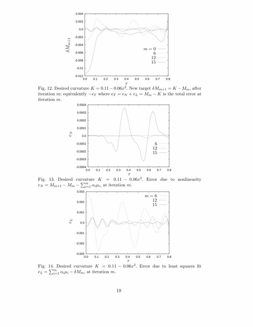
8 Example: Quadratic Curvature

Obtaining a constant curvature on the glass by thermal replication is, practi-cally speaking, unrealistic since there are better ways to obtain such a surface.Hence we consider the more realistic task of determining the former shape togive a quadratic curvature profile across the radius of the glass, with high-est curvature in the centre, lowest curvature at the edge. Since we are takingcurvature to be the second derivative, this means the former will be approx-imately described by a quartic polynomial. We consider the initial formerelevation profile

F (r) = 0.05(r2 − 1)(1 − 0.1r2)

which gives a maximum cavity depth of d = 0.05 at the centre as for thespherical former already considered. We continue to use an initially flat glassdisc with h = 0.1333 and we take F (r) to be the zeroth-order former solutionfor the desired curvature profile on the glass K = (F + h)′′, i.e. the quadraticcurvature profile

K = 0.11 − 0.06r2.

Note that this is a slightly different and less accurate definition of the zeroth-order solution than discussed earlier, obtained by simply translating the de-sired top surface of the glass vertically down by an amount equal to the glassthickness. Thus, we are starting with a less accurate estimate of the former ge-ometry for our desired curvature profile compared to that used in the previousexample.

Apart from the changed initial former geometry and desired curvature profile,we proceed exactly as for the previous example. Our results are shown inFigures 12–14. As for the constant curvature example considered first, anexcellent solution is obtained after twelve iterations, after which error due tononlinearity begins to grow and impact strongly on the results. As a result,the total error at m = 13 reduces a little compared to that at m = 12 but thenincreases substantially at m = 14. Depending on the importance of reducingerror near r = 0.8, the solution at iteration m = 15 might be considered betterthan that at m = 12 or 13, but at subsequent iterations the error due tononlinearity, and hence the total error, grows by several orders of magnitude.

The curves of new target δMm+1, error due to nonlinearity eN and error dueto least-squares fitting eL are quite similar in both appearance and magnitudefor both examples, despite the fact that we started with a less accurate es-timate of the solution for the quadratic-curvature case (compare the curvesfor m = 0, i.e. the initial error, in Figures 9 and 12). In both examples thegrowth in nonlinearity eventually prevents further improvment in the solutionby including smaller wavelength perturbations in our basis set and continuingto iterate.

17

-0.012

-0.01

-0.008

-0.006

-0.004

-0.002

0.0

0.002

0.004

0.0 0.1 0.2 0.3 0.4 0.5 0.6 0.7 0.8

δMm

+1

r

m = 06

1215

Fig. 12. Desired curvature K = 0.11− 0.06x2. New target δMm+1 = K −Mm, afteriteration m; equivalently −eT where eT = eN + eL = Mm − K is the total error atiteration m.

-0.0004

-0.0003

-0.0002

-0.0001

0.0

0.0001

0.0002

0.0003

0.0004

0.0 0.1 0.2 0.3 0.4 0.5 0.6 0.7 0.8

e N

r

61215

Fig. 13. Desired curvature K = 0.11 − 0.06x2. Error due to nonlinearityeN = Mm+1 − Mm −

∑mi=1 αiµi, at iteration m.

-0.003

-0.002

-0.001

0.0

0.001

0.002

0.003

0.0 0.1 0.2 0.3 0.4 0.5 0.6 0.7 0.8

e L

r

m = 61215

Fig. 14. Desired curvature K = 0.11 − 0.06x2. Error due to least squares fiteL =

∑mi=1 αiµi − δMm, at iteration m.

18

9 Conclusions

We have applied the finite-element method to the Stokes Equation in orderto solve the inverse problem of slumping of molten glass. This is a highlynonlinear problem. The slumping time required to achieve full contact, wasdetermined first as achieving full contact between glass and former was foundto be important to minimise nonlinearity. Then the shape of the ceramic for-mer that produces a prescribed top surface curvature profile was sought, usinga variant of the multivariable Newton-Raphson method. Choosing an appro-priate set of basis perturbation functions for the former, a corresponding setof perturbation functions for the upper free surface of the glass is obtainedby solving the forward slumping problem for each of the former perturbationfunctions. Then the lower former surface and desired upper free surface on theglass can be approximated by linear combinations of each of these sets of basisfunctions respectively. Thus the mapping is reduced to the finite-dimensionalproblem of solving for the set of coefficients in these linear combinations.Gramm-Schmidt orthogonalisation of the perturbation functions for the glasswas carried out, to reduce the effect of nonlinear interaction.

We have studied the effect of the various parameters on the nonlinearity of thismapping. The nonlinearity was found to increase with the ratio of the glassthickness to the perturbation scale. Short-scale perturbations and thick glass,increase the nonlinearity. The steepness of the perturbation also increases non-linearity. One of the challenges was to maintain a sufficient number of degreesof freedom to represent the required surfaces, while avoiding the strongly non-linear short scales. This was achieved by introducing ‘hump shaped’ basisfunctions. These, being localized, also had (in general) less nonlinear interac-tions among them than, say, full cosine perturbations.

It is preferable to remove first the long-scale perturbations. These have largeramplitudes, for a given steepness, and behave more linearly. However, theyinteract in a strongly nonlinear way with shorter perturbations. Once thelong-scale errors are reduced, the short-scale errors are easier to eliminate.Increasingly shorter-scale perturbations were gradually added.

The residual errors are largest near the outer edge of the former, which is usu-ally trimmed in the industrial process. In fact, in addition to determining theformer geometry to achieve the desired glass product, we can also determinethe extent of edge trimming required for a given tolerance profile on the finalproduct. Our results indicate that a trimming value of r = 0.8 is a reasonablechoice.

This process reduced the error in curvature, within 12 iterations, from a mag-nitude of 1.3 × 10−2 (1.1 × 10−2) to 3.5 × 10−4 (3.8 × 10−4) at the centre and

19

6.1 × 10−3 (3.0 × 10−3) to 6.2 × 10−4 (4.3 × 10−4) at r = 0.75 for the con-stant (quadratic) curvature case. After 12 iterations, the maximum error over0 ≤ r ≤ 0.75 was 6.2 × 10−4 (6.3 × 10−4) at r = 0.75 (0.64) respectively; itincreases to 1.6 × 10−3 (1.3 × 10−3) at r = 0.8 where trimming would almostcertainly be appropriate. While these are excellent results, modifications maybe required if there is need to further reduce the error, especially at shorterscales. Strategies for enhancing the method are currently being explored.

Acknowledgements

This research was supported by The Fund for the Promotion of Research atthe Technion and a visit by YMS to the Technion was supported by the SwissFund. YMS thanks YA for both financial support and hospitality while visitingthe Technion.

A Computational algorithm

Final computational algorithm for determining the former F (r, θ) for the de-sired curvature profile K(r, θ):

1. Estimate/guess the former profile F0(r, θ) that will yield K.F0(r, θ) ⇒ M0(r, θ).

2. Do m = 1, N2.1 Target δMm = K − Mm−1.2.2 If |δMm| < tolerance, 0 ≤ r ≤ b then stop.2.3 Do i = 1, m

(a) Fm−1 + δi ⇒ Mm−1 + µi.(b) Do j=1, 1(2, 3)

(i) νi ⇐ µi, γi ⇐ δi

(ii) Do k = 1, (i − 1)

νi ⇐ νi −(νi · νk)νk

‖νk‖, γi ⇐ γi −

(νi · νk)γk

‖νk‖.

(iii) δi ⇐ γi, Fm−1 + δi ⇒ Mm−1 + µi

2.4 Solve δMm ≈m∑

i=1

αiµi for αi, i = 1, . . . ,m.

2.5 Fm = Fm−1 +m∑

i=1

αiδi.

2.6 Fm ⇒ Mm

20

References

[1] F.M. Duarte and J.A. Covas, IR sheet heating in roll fed thermoforming Part 1- Solving direct and inverse heating problems, Plast. Rubber Compos. 31 (2002)307–317.

[2] F.M. Duarte and J.A. Covas, Infrared sheet heating in roll fed thermoformingPart 2 - Factors influencing inverse heating solution, Plast. Rubber Compos. 32(2003) 32–39.

[3] H.W. Engl and P. Kugler, The influence of the equation type on iterativeparameter identification problems which are elliptic or hyperbolic in theparameter, Eur. J. Appl. Math. 14 (2003) 129-163.

[4] P.D. Howell, Models for thin viscous sheets, Eur. J. Appl. Math. 9 (1998) 93–93.

[5] R. Hunt, Numerical solution of the flow of thin viscous sheets under gravityand the inverse windscreen sagging problem, Int. J. Numer. Meth. Fl. 38 (2002)533-553.

[6] M. Hyre, Numerical simulation of glass forming and conditioning, J. Amer.Ceramic Soc. 85 (2002) 1047–1056.

[7] M.S. Joun and S.M. Hwang, Die shape optimal design in three-dimensionalshape metal extrusion by the finite element method, Int. J. Numer. Meth. Eng.42 (1998) 1343–1390.

[8] K. Laevsky and R.M.M. Mattheij, Determining the velocity as a kinematicboundary condition in a glass pressing problem, J. Comp. Meth. Sci. Eng. 2(2003) 285–298.

[9] H.M. Pollicove, Survey of present lens molding techniques, In Riedl, M.J.(ed), Replication and Molding of Optical Components, Vol 896, Proceedingsof The Society of Photo-Optical Instrumentation Engineers, Washington, 1988,pp. 158–159.

[10] H. Scholze and N.J. Kreidl, Technological aspects of viscosity, In Uhlmann,D.R. and Kreidl, N.J. (eds), Glass Science and Technology, Vol 3 Viscosity andRelaxation, Academic Press, Orlando, 1986, pp. 233–273.

[11] N. Siedow and M. Brinkmann, Direct and inverse temperature reconstructionof hot glass, in Proceedings of the 2nd International Colloquium “Modelling ofGlass Forming and Tempering”, Valenciennes 23 - 25 January 2002, pp. 173-177.

[12] L. Smith, R.J. Tillen and J. Winthrop, New directions in aspherics: glass andplastic, in Riedl, M.J. (ed), Replication and Molding of Optical Components,Vol 896, Proceedings of The Society of Photo-Optical InstrumentationEngineers, Washington, 1988, pp. 160–166.

[13] L.C. Sousa, C.F. Castro, C.A.C. Antonio and A.D. Santos, Inverse methodsin design of industrial forging processes, J. Mater. Process. Tech. 128 (2002)266–273.

21

[14] J. Sprekels, H. Goldberg and F. Troltzsch, Numerical treatment ofa shape optimization problem in thermoelasticity, DFG-Preprint series“Anwendungsbezogene Optimierung und Steuerung”, Report No. 520.

[15] Y.M. Stokes, Thermal replication: a comparison of numerical and experimentalresults, in Tuck, E.O., Stott, J.A.K. (eds) Proceedings of the 3rd BiennialEngineering Mathematics and Applications Conference: EMAC98, Institutionof Engineers, Australia, 1998, pp. 471–474.

[16] Y.M. Stokes, Very viscous flows driven by gravity with particular applicationto slumping of molten glass, PhD Thesis, Department of Applied Mathematics,University of Adelaide, July 1998.

[17] Y.M. Stokes, Numerical design tools for thermal replication of optical surfaces,Comput. Fluids 29 (2000) 401–414.

[18] E.O. Tuck, Y.M. Stokes and L.W. Schwartz, Slow slumping of a very viscousliquid bridge, J. Eng. Math. 32 (1997) 27–40.

[19] B.W. van de Fliert, P.D. Howell and J.R. Ockendon, Pressure-driven flow of athin viscous sheet, J. Fluid Mech. 292 (1995) 359–376.

[20] C.H. Wang and H.F. Nied, Temperature optimization for improved thicknesscontrol in thermoforming, J. Mater. Process. Manu. 8 (1999) 113–126.

[21] X. Zhao, G. Zhao, G. Wang and T. Wang, Preform die shape design foruniformity of deformation in forging based on preform sensitivity analysis, J.Mater. Process. Tech. 128 (2002) 25–32.

22