an inversion of acoustical attenuation measurements to

An Inversion of Acoustical Attenuation Measurements to Deduce Bubble Populations

H. CZERSKI

Institute of Sound and Vibration Research, University of Southampton, Highfield, Southampton, United Kingdom

(Manuscript received 16 September 2011, in final form 3 February 2012)

ABSTRACT

Measurement of natural bubble populations is required for many areas of ocean science. Acousticalmethods have considerable potential for achieving this goal because bubbles scatter sound strongly close totheir natural frequency, which depends largely on the bubble radius. The principle of using bulk acousticalattenuation caused by a bubble population to infer the number and size of bubbles present is well established,and appropriate methods for measuring broadband acoustical attenuation are also well developed. However,the numerical methods currently used to invert the acoustical attenuation to get the bubble size distributionare complex and time consuming. In this paper, a method for the inversion is presented that uses the physics ofbubble resonance to restructure the problem so that it can be accurately carried out using a simple matrixinversion. This inversion method produces results that are correct to within a few percent over two orders ofmagnitude of bubble size. The most significant remaining issue for acoustical bubble measurement is thepotential presence of bubbles that are resonant outside the measurement frequency range. The mathematicalstructure outlined here considerably simplifies the investigation of this problem, and calculations are pre-sented that show this effect to be minor in many cases.

1. Introduction

The presence of bubbles in a liquid can have a consid-erable influence on that liquid’s optical and acousticalproperties, as well as providing opportunities for the ex-change of gases across the bubble boundary. Conse-quently, accurate measurement of the number and sizeof the bubbles present is desirable in many fields ofscience, for example, chemical engineering, medicine,and oceanography. The aim of the research presented inthis paper is to improve the measurement of the naturalbubble populations in the ocean, and it was motivated bythe increasing interest in measuring bubbles with radiiless than 50 mm. However, the principle described maybe useful in other applications as well.

It is now four decades since Medwin (1970) introducedthe concept of measuring oceanic bubble populations byusing the bulk acoustical properties of the bubbly water toinfer the bubble size distribution present. The mainadvantages of the technique are that the instrumentationis relatively simple, nonintrusive, and robust enough to be

deployed in rough conditions at sea. In addition, mea-surements can be made continuously at 1 Hz or faster,which is sufficient to follow the evolution of bubble cloudsfrom a breaking wave once the initial intense period ofturbulence and very high void fraction is over. Over thelength of time that this technique has been in use, therehave been several proposed methods for inverting theacoustical attenuation to infer the bubble populationpresent. The reason for this is that even though thecontribution to acoustical attenuation made by a singlesize of bubble is greatest at its natural frequency, theeffects at other frequencies may still be significant. Thiscomplicates the calculation of the bubble size distribu-tion, and to date a universally satisfactory method forcarrying out the inversion has not been found.

Medwin (1977) and Breitz and Medwin (1989) laid thetheoretical foundations for the inversion process. Twoequivalent sets of units are used in the literature foracoustical attenuation: decibels, which are commonlyused by acousticians, and a pressure amplitude attenu-ation coefficient b in nepers per meter, which is morecommonly used by physicists. Here we will use b be-cause it is simpler to express, but both will be set outbelow for clarity. The total acoustical power attenua-tion adB in decibels per meter at a given frequency f isexpressed as

Corresponding author address: H. Czerski, Institute for Soundand Vibration Research, Highfield, University of Southampton,SO17 1BJ, United Kingdom.E-mail: [email protected]

AUGUST 2012 C Z E R S K I 1139

DOI: 10.1175/JTECH-D-11-00170.1

! 2012 American Meteorological Society

adB( f ) 5 4:34

ð‘

0sext( f , a)n(a) da, (1a)

where n(a)da is the number of bubbles with radii betweena and a 1 da per unit volume. The factor of 4.34 comesfrom the conversion to decibels (Medwin 2005; Leighton1994, p. 28), where I 5 I0102(adBx=10), where I0 and I arethe initial and final intensities and x is the distance trav-eled. For calculations using the construction I 5 I0e2ax,this factor is not needed, and the attenuation referred toin this paper will be calculated in this way. In these units,the power attenuation coefficient a is given by a 5 2b, sothat the correct version of Eq. (1) for our purposes is

a( f ) 5ð‘

0sext( f , a)n(a) da. (1b)

The extinction cross section sext(v, a0) resulting from abubble of radius a0 at angular frequency v (where v 52pf ) is given by Eqs. (4.27) and (4.31) in Leighton (1994) as

sext(v, a0) 5dtot

drad

4pa20"

v0

v

# $22 1

%21

2btot

v

& '2, (2)

where dtot is the total damping constant, drad is theradiation damping constant, a0 is the bubble equilibriumradius, v0 is its resonant frequency, v is the frequency ofinterest, and btot is the total resistive constant leading todamping. Equation (2) is a complete description of theacoustical extinction and includes both resonant andgeometric effects. Geometric scattering is that due to thepurely cross-sectional area of the bubble, separate fromany resonant effects, and it increases as a2

0. In theory, ifthe attenuation with frequency is known, Eqs. (1) and

(2) could be inverted to calculate n(a)da. Consequently,a single broadband measurement could be used to inferthe bubble population over a wide radius range.

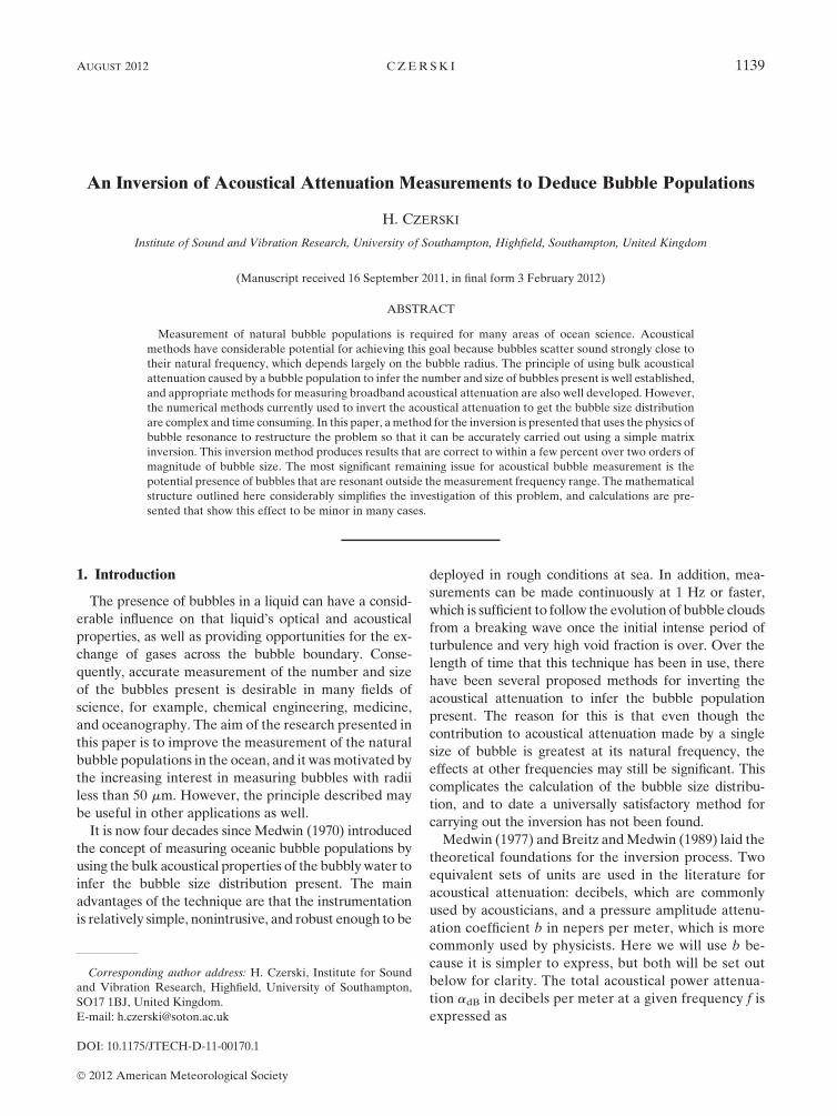
Figure 1 shows two aspects of the extinction crosssection: the variation with radius at a single frequency(217 kHz) and the variation with frequency for a bubble offixed radius (15 mm). The steadily rising slope on the rightof the resonant peak in Fig. 1a represents geometric scat-tering, which is the acoustic scattering resulting from thephysical size of a bubble (Leighton 1994). The difficultythat this geometric scattering causes is that at a single rel-atively high frequency, attenuation can potentially be dueto either small resonant bubbles or the geometric scattering(effectively the acoustic shadow) from a range of muchlarger bubbles. Figure 1b illustrates that a bubble of a singlesize causes attenuation over a narrow range of frequencies,not just its resonant frequency. Here, this range is referredto as the bubble bandwidth. A solution to Eqs. (1) and (2)must take both of these features into account.

A solution to first order was derived by Medwin (1977),by assuming that the measured attenuation was domi-nated by resonant scattering only (commonly referred toas the resonant bubble approximation). A simplifiedexpression was derived that directly related measuredattenuation to the number of resonant bubbles present.The limitations of this approach were investigated byCommander and Moritz (1989), and they concluded thatthe off-resonant contributions to scattering needed to beincluded in future inversion methods.

Several methods have been proposed to take theoff-resonant contributions into account. The most widelyused method (Terrill and Melville 2000; Farmer et al.1998) is that of Commander and McDonald (1991). Notingthat Eq. (1) is a Fredholm integral of the first kind, they

FIG. 1. Extinction cross sections: (a) variation in cross section with radius for 217 kHz, which is the resonantfrequency for a 15-mm bubble, and (b) variation with frequency for a single bubble with a radius of 15 mm.

1140 J O U R N A L O F A T M O S P H E R I C A N D O C E A N I C T E C H N O L O G Y VOLUME 29

found a numerical solution to the integral by using afinite-element method, and then regularization was usedto produce a stable result. This method is computationallyexpensive, since it requires an iterative procedure tosmooth the result.

Caruthers et al. (1999) and Elmore and Caruthers(2003) proposed and developed a simpler alternativesolution. They used the resonant approximation toproduce a first-order solution and then made iterativecorrections using the full forward attenuation calcula-tion. A different numerical solution using both attenu-ation and phase velocity was developed by Duraiswamyet al. (1998). Choi and Yoon (2001) also proposed aniterative scheme using both the attenuation and thephase velocity to find a stable result.

In general, these methods are all computationallyexpensive and time consuming to carry out. In addition,these studies all have two things in common. First, they allset out to produce a general mathematical solution toEq. (1), without considering the physical phenomenadescribed by the kernel s. Consideration of the physicalmeaning of that term and the shape of the function itdescribes leads to a solution specific to bubble inversion.Previous solution methods have been inefficient becausethey have all been very general mathematical treatmentsthat would work for any kernel. Second, in the caseswhere an artificial bubble population was simulated anda full forward calculation of attenuation was carried outso that the inversion method could be tested, the issue ofbinning bubbles before the attenuation was calculatedwas not addressed, as far as the author is aware. Duringconsideration of possible inversion methods for bubblemeasurements using an acoustical resonator, it becameapparent that there is a simpler method for inversion,which takes account of the two points above and isconsiderably quicker to implement than previousmethods. In addition, it removes some systematic errorsthat may have been overlooked in previous inversions.

2. Method description

As discussed above, the attenuation resulting from asingle bubble resonance is significant over a finite fre-quency range, quantified by the bandwidth of the bubbleresonance. Consequently, the attenuation measured at anysingle frequency is a sum of attenuation caused by bubbleswith a resonant response close to the frequency of mea-surement and possibly also attenuation caused by geome-tric scattering from larger bubbles. Figure 2 demonstratesthe problem for a flat bubble distribution (i.e., one forwhich there are equal numbers of bubbles in each radiusincrement). The acoustic cross section is shown with fre-quency for several bubbles at equal radius increments

around 3 mm in radius. The total measured attenuation willbe proportional to the sum of all of these cross sections, andit can be seen that the resonance width is a crucial pa-rameter in determining how much overlap there is betweenbubbles separated by a fixed radius increment. This reso-nant bandwidth depends on the damping associated withthe resonance. For all the calculations described in thispaper, the damping coefficients were calculated usingProsperetti’s (1977) method. For bubbles with smallerradii (which resonate at higher frequencies), this resonantbandwidth is generally greater than that for larger bub-bles. There is a small contribution to this bandwidth in-crease from the decrease in resonance quality factor asbubbles get smaller, but most of the bandwidth increase isjust due to the definition of quality factor,

Q 5v0

Dv, (3)

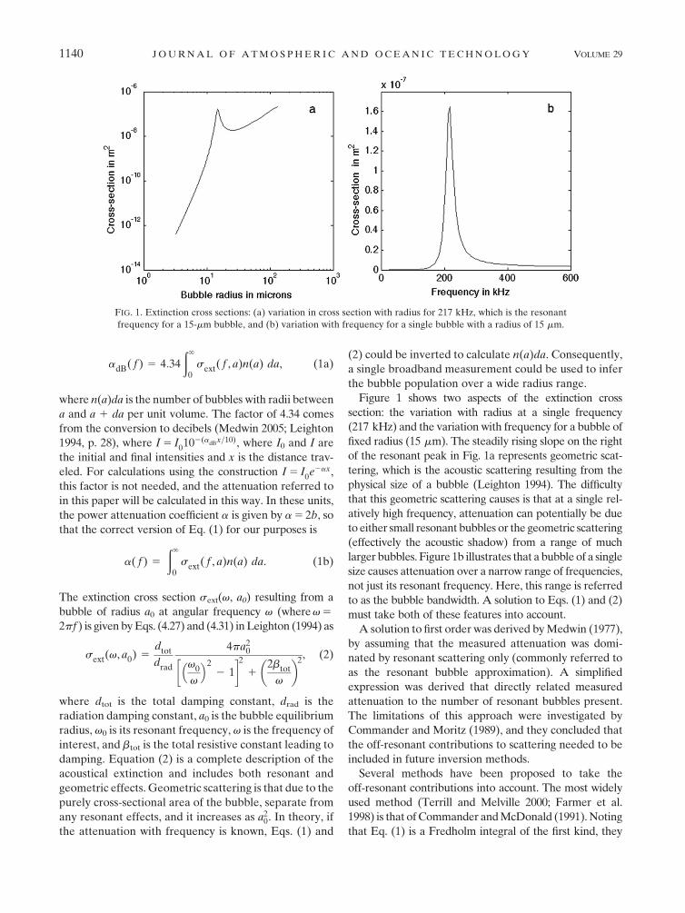
where Q is the bubble resonance quality factor, v0 is itsresonant angular frequency, and Dv is the resonancebandwidth. As the resonant frequency increases, thebandwidth increases for the same quality factor. Figure 3shows the normalized cross sections with frequency forfour different bubble sizes. Each one is normalized to itsmaximum value.

Most attenuation measurements are equally spaced infrequency space, and it is evident from Fig. 3 that there areimplications for the inversion if inversion points werechosen with this equal frequency spacing. An attenuationmeasurement at the lower frequencies would be influ-enced by only a small number of the bubbles in the cor-responding bin, while at the higher frequencies theattenuation measurement would include a significantportion from bubbles in other bins. It seems that this ap-proach could generate a systematic error. Most previouspublications do not discuss the spacing of the inversionpoints used, but a large part of the effort that has been

FIG. 2. A sample plot of the many individual cross sections thatmight add up to form the total attenuation. Most of the measuredattenuation is due to bubbles that are not responding exactly attheir resonance frequency, but resonate within approximatelya bandwidth of the frequency of interest.


expended on the inversion of Eq. (1) is compensating forthis effect. It also seems to be the major reason for thefailure of singular value decomposition inversion methodsto produce stable solutions; if the inversion points arechosen with equal frequency spacing, then there aremany possible combinations at the higher frequenciesthat can produce the same overall attenuation. Thismeans that the matrix inversion does not have a uniquesolution and no stable result can be found.

The central theme of this paper is that the inversionaccuracy and stability will be considerably improved ifthe spacing of the points used in the inversion is chosen sothat the frequency bins each have a width in frequencyspace that matches the bandwidth of their central bubble.Figure 4 shows part of the frequency spectrum split up intobins with this spacing. Using this method, every bubble willbe resonant in a bin (so the full forward attenuation cal-culation will include the correct number of bubbles), butthe bin width reflects the frequency range that can beinfluenced by the bubbles inside that bin. This means thata matrix inversion method can be used, and that thesolution will be smooth and stable because the mathe-matical construction reflects the physics of the process.

The bandwidth of each bubble resonance can be de-rived by comparing Eq. (3) with Eq. (2); 1=Q is equivalentto 2btot=v0, so the width of each bin in hertz is given by

Df 5btot

p. (4)

Prosperetti’s (1977) method is used to calculate theacoustic, thermal, and viscous effective viscosities m.Then, btot was calculated using Eq. (5) as

btot 52(mviscous 1 macoustic 1 mthemal)

rwatera20

, (5)

where rwater is the density of the liquid and a0 is thebubble radius.

Once the central bin frequencies are known, thena matrix of cross-sectional contributions can be calculatedfor these frequencies and the corresponding bubble radiiby using Eq. (2). The resulting matrix equation is

2

664

s(a1, f1) s(a2, f1) s(a3, f1) . . .s(a1, f2) s(a2, f2) s(a1, f2)s(a1, f3) s(a2, f3) s(a1, f3)

. . .

3

775

2

664

n(a1)n(a2)n(a3). . .

3

775 5

2

664

a( f1)a( f2)a( f3). . .

3

775, (6)

where fi are the central frequencies of the frequency bins,and ai are the radii of the resonant bubbles at those fre-quencies. The values of a( fi) are interpolated from themeasured data points, and this matrix equation is solvedusing singular value decomposition to get the values n(ai).

The final stage is to divide the calculated n(ai) by thenumber of micron radius increments that are included inthe corresponding frequency bin to get the bubblenumber per unit volume per micron radius increment.

3. Method justification

If there were no geometrical scattering by larger bub-bles, this method would just consist of dividing the atten-uation at the center frequency of each bin by the resonantcross section of the central bubble. The reason that a ma-trix formulation is needed is to take into account thegeometrical scattering caused by bubbles larger than thosein the bin of interest. Even though the matrix inversion is

FIG. 3. The variation of extinction cross section with frequencyfor different bubble sizes, normalized to their maximum value. Thebubble radii are (a) 50, (b) 20, (c) 10, and (d) 5 mm.

FIG. 4. A region of the spectrum showing the suggested fre-quency bin spacing and the cross section of the central bubble foreach bin. Dotted vertical lines represent the frequency boundariesfor the bins. The attenuation values used in the inversion will be atthe frequency of the center of each bin (black filled circles), usinginterpolation between the measured acoustic data points.


stable, we have not yet shown this will give the correctnumber of bubbles in the bin rather than a value that isproportional to the correct number. However, a simplephysical argument presented in this section and the resultsin section 4 show that this is indeed the case. Considera bubble in a frequency bin that is not necessarily resonantat the central frequency of that bin. There will also beattenuation at the measurement frequency from bubblesin the bins on either side, although their contribution willnot dominate the measured attenuation. Let us supposethat for each bubble in a bin, we can find another bubblethat is resonant at one bandwidth above, and a third that isresonant one bandwidth below the bubble of interest (sothese two are contained within the bins on either side ofthe bin of interest), and that the influence of any otherbubbles is small. We will call the bubble of interest herethe ‘‘middle bubble’’ of the three, to distinguish it from thecentral bubble of the bin. It is a reasonable assumption fora continuous distribution that two such symmetrical cor-responding bubbles can be found for any single middlebubble. Figure 5 shows this situation. The peak resonanceof the middle bubble can be anywhere inside the bin. Theaverage contribution that a bubble in this bin would makeis therefore the mean value of the total attenuation at all

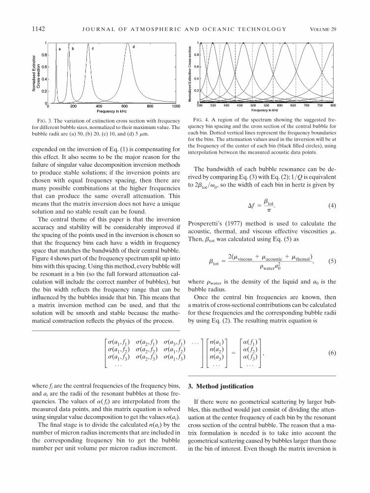
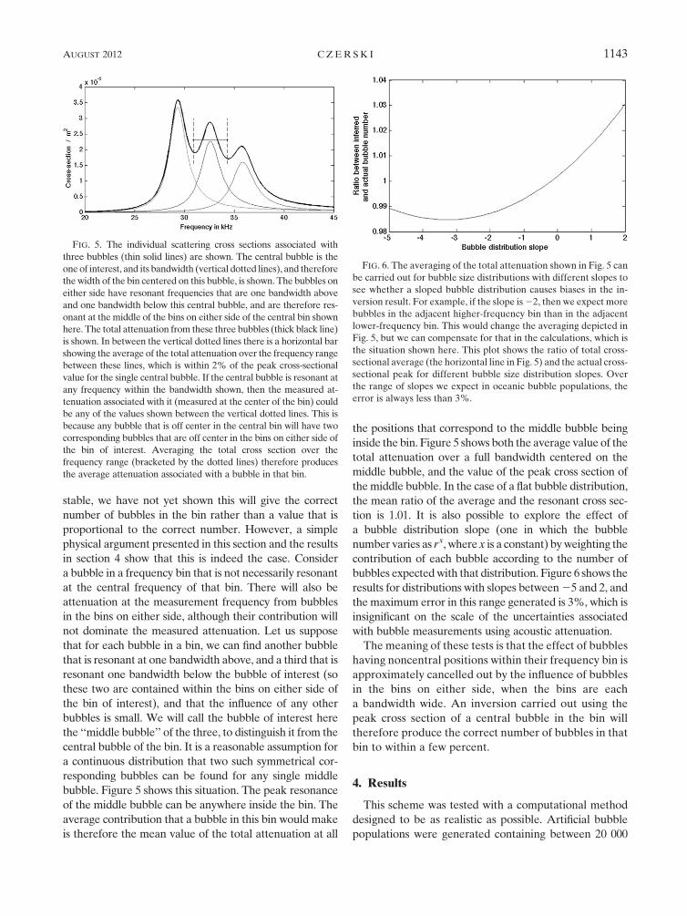
the positions that correspond to the middle bubble beinginside the bin. Figure 5 shows both the average value of thetotal attenuation over a full bandwidth centered on themiddle bubble, and the value of the peak cross section ofthe middle bubble. In the case of a flat bubble distribution,the mean ratio of the average and the resonant cross sec-tion is 1.01. It is also possible to explore the effect ofa bubble distribution slope (one in which the bubblenumber varies as rx, where x is a constant) by weighting thecontribution of each bubble according to the number ofbubbles expected with that distribution. Figure 6 shows theresults for distributions with slopes between 25 and 2, andthe maximum error in this range generated is 3%, which isinsignificant on the scale of the uncertainties associatedwith bubble measurements using acoustic attenuation.

The meaning of these tests is that the effect of bubbleshaving noncentral positions within their frequency bin isapproximately cancelled out by the influence of bubblesin the bins on either side, when the bins are eacha bandwidth wide. An inversion carried out using thepeak cross section of a central bubble in the bin willtherefore produce the correct number of bubbles in thatbin to within a few percent.

4. Results

This scheme was tested with a computational methoddesigned to be as realistic as possible. Artificial bubblepopulations were generated containing between 20 000

FIG. 5. The individual scattering cross sections associated withthree bubbles (thin solid lines) are shown. The central bubble is theone of interest, and its bandwidth (vertical dotted lines), and thereforethe width of the bin centered on this bubble, is shown. The bubbles oneither side have resonant frequencies that are one bandwidth aboveand one bandwidth below this central bubble, and are therefore res-onant at the middle of the bins on either side of the central bin shownhere. The total attenuation from these three bubbles (thick black line)is shown. In between the vertical dotted lines there is a horizontal barshowing the average of the total attenuation over the frequency rangebetween these lines, which is within 2% of the peak cross-sectionalvalue for the single central bubble. If the central bubble is resonant atany frequency within the bandwidth shown, then the measured at-tenuation associated with it (measured at the center of the bin) couldbe any of the values shown between the vertical dotted lines. This isbecause any bubble that is off center in the central bin will have twocorresponding bubbles that are off center in the bins on either side ofthe bin of interest. Averaging the total cross section over thefrequency range (bracketed by the dotted lines) therefore producesthe average attenuation associated with a bubble in that bin.

FIG. 6. The averaging of the total attenuation shown in Fig. 5 canbe carried out for bubble size distributions with different slopes tosee whether a sloped bubble distribution causes biases in the in-version result. For example, if the slope is 22, then we expect morebubbles in the adjacent higher-frequency bin than in the adjacentlower-frequency bin. This would change the averaging depicted inFig. 5, but we can compensate for that in the calculations, which isthe situation shown here. This plot shows the ratio of total cross-sectional average (the horizontal line in Fig. 5) and the actual cross-sectional peak for different bubble size distribution slopes. Overthe range of slopes we expect in oceanic bubble populations, theerror is always less than 3%.


and 200 000 bubbles, with a distribution of sizes that fit thechosen bubble population distribution. The populationwas constructed by finding the number of bubbles re-quired in each micron radius increment at radius R inorder to fit the distribution. A random number between0 and 1 (designated B) was generated for each individualbubble, and that bubble was given a radius r 5 R 1 BDr,where Dr is 1 mm. Significantly, this meant that manydifferent bubble radii were included within each fre-quency bin used for the inversion. ‘‘Measurement’’ fre-quencies were chosen, and the total attenuation wascalculated at each chosen frequency by using the exactbubble radii for each bubble without any binning. This isequivalent to carrying out the sum represented by theintegral in Eq. (1). This attenuation was then invertedusing the method described here to test its accuracy.

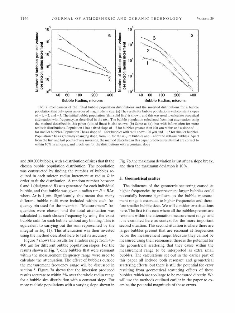
Figure 7 shows the results for a radius range from 40–400 mm for different bubble population slopes. For theresults shown in Fig. 7, only bubbles that were resonantwithin the measurement frequency range were used tocalculate the attenuation. The effect of bubbles outsidethe measurement frequency range will be discussed insection 5. Figure 7a shows that the inversion producedresults accurate to within 2% over the whole radius rangefor a bubble size distribution with a constant slope. Formore realistic populations with a varying slope shown in

Fig. 7b, the maximum deviation is just after a slope break,and then the maximum deviation is 10%.

5. Geometrical scatter

The influence of the geometric scattering caused athigher frequencies by nonresonant larger bubbles couldpotentially become significant as the bubble measure-ment range is extended to higher frequencies and there-fore smaller bubble sizes. We will consider two situationshere. The first is the case where all the bubbles present areresonant within the attenuation measurement range, andit is examined here as context for the more importantsecond situation. This second situation is where there arelarger bubbles present that are resonant at frequenciesbelow the measurement range. Because they cannot bemeasured using their resonance, there is the potential forthe geometrical scattering that they cause within themeasurement range to be interpreted as extra smallbubbles. The calculations set out in the earlier part ofthis paper all include both resonant and geometricalscattering effects, but there is still the potential for errorresulting from geometrical scattering effects of thesebubbles, which are too large to be measured directly. Wewill use the methods outlined earlier in the paper to ex-amine the potential magnitude of these errors.

FIG. 7. Comparison of the initial bubble population distributions and the inverted distributions for a bubblepopulation that only spans an order of magnitude in size. (a) The results for bubble populations with constant slopesof 21, 22, and 23. The initial bubble population (thin solid line) is shown, and this was used to calculate acousticalattenuation with frequency, as described in the text. The bubble population calculated from that attenuation usingthe method described in this paper (dotted lines) is also shown. (b) Same as (a), but with information for morerealistic distributions. Population 1 has a fixed slope of 23 for bubbles greater than 100-mm radius and a slope of 21for smaller bubbles. Population 2 has a slope of 24 for bubbles with radii above 100 mm and 21.5 for smaller bubbles.Population 3 has a gradually changing slope, from 21 for the 40-mm bubbles and 24 for the 400-mm bubbles. Apartfrom the first and last points of any inversion, the method described in this paper produces results that are correct towithin 10% in all cases, and much less for the distributions with a constant slope


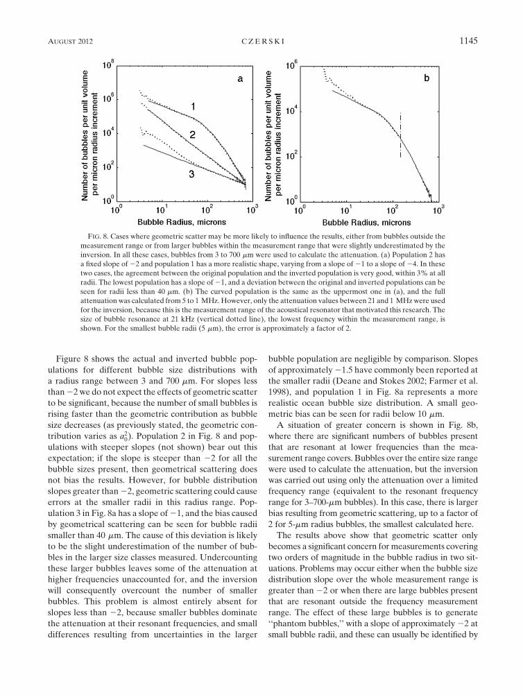
Figure 8 shows the actual and inverted bubble pop-ulations for different bubble size distributions witha radius range between 3 and 700 mm. For slopes lessthan 22 we do not expect the effects of geometric scatterto be significant, because the number of small bubbles isrising faster than the geometric contribution as bubblesize decreases (as previously stated, the geometric con-tribution varies as a2

0). Population 2 in Fig. 8 and pop-ulations with steeper slopes (not shown) bear out thisexpectation; if the slope is steeper than 22 for all thebubble sizes present, then geometrical scattering doesnot bias the results. However, for bubble distributionslopes greater than 22, geometric scattering could causeerrors at the smaller radii in this radius range. Pop-ulation 3 in Fig. 8a has a slope of 21, and the bias causedby geometrical scattering can be seen for bubble radiismaller than 40 mm. The cause of this deviation is likelyto be the slight underestimation of the number of bub-bles in the larger size classes measured. Undercountingthese larger bubbles leaves some of the attenuation athigher frequencies unaccounted for, and the inversionwill consequently overcount the number of smallerbubbles. This problem is almost entirely absent forslopes less than 22, because smaller bubbles dominatethe attenuation at their resonant frequencies, and smalldifferences resulting from uncertainties in the larger

bubble population are negligible by comparison. Slopesof approximately 21.5 have commonly been reported atthe smaller radii (Deane and Stokes 2002; Farmer et al.1998), and population 1 in Fig. 8a represents a morerealistic ocean bubble size distribution. A small geo-metric bias can be seen for radii below 10 mm.

A situation of greater concern is shown in Fig. 8b,where there are significant numbers of bubbles presentthat are resonant at lower frequencies than the mea-surement range covers. Bubbles over the entire size rangewere used to calculate the attenuation, but the inversionwas carried out using only the attenuation over a limitedfrequency range (equivalent to the resonant frequencyrange for 3–700-mm bubbles). In this case, there is largerbias resulting from geometric scattering, up to a factor of2 for 5-mm radius bubbles, the smallest calculated here.

The results above show that geometric scatter onlybecomes a significant concern for measurements coveringtwo orders of magnitude in the bubble radius in two sit-uations. Problems may occur either when the bubble sizedistribution slope over the whole measurement range isgreater than 22 or when there are large bubbles presentthat are resonant outside the frequency measurementrange. The effect of these large bubbles is to generate‘‘phantom bubbles,’’ with a slope of approximately 22 atsmall bubble radii, and these can usually be identified by

FIG. 8. Cases where geometric scatter may be more likely to influence the results, either from bubbles outside themeasurement range or from larger bubbles within the measurement range that were slightly underestimated by theinversion. In all these cases, bubbles from 3 to 700 mm were used to calculate the attenuation. (a) Population 2 hasa fixed slope of 22 and population 1 has a more realistic shape, varying from a slope of 21 to a slope of 24. In thesetwo cases, the agreement between the original population and the inverted population is very good, within 3% at allradii. The lowest population has a slope of 21, and a deviation between the original and inverted populations can beseen for radii less than 40 mm. (b) The curved population is the same as the uppermost one in (a), and the fullattenuation was calculated from 5 to 1 MHz. However, only the attenuation values between 21 and 1 MHz were usedfor the inversion, because this is the measurement range of the acoustical resonator that motivated this research. Thesize of bubble resonance at 21 kHz (vertical dotted line), the lowest frequency within the measurement range, isshown. For the smallest bubble radii (5 mm), the error is approximately a factor of 2.


an inflection in the bubble slope at the radius at which theinverted population starts to differ from the actual bubblepopulation. These indications may suggest, after the in-version has been done, that geometric scattering isa problem. No direct solution for this problem is offeredhere, although some straightforward modeling based onthe individual populations measured could provideenough information to rule out geometrical scattering asa problem in some cases. For example, as shown in Fig.8b, the population of larger bubbles that resonates out-side the ‘‘measured’’ frequency range could reasonablyhave a slope between 23 and 25. A simple forward cal-culation of the attenuation generated by the postulatedlarge bubbles over the whole frequency range, followedby inversion using only the measurement frequencyrange, shows the number of phantom bubbles that thepresence of larger bubbles could generate. An estimate oftheir importance can then be made. In the cases studiedby the author using real bubble populations, the steepnessof the bubble size distribution at the largest radii usuallysuggests that geometric scattering does not bias the in-version results. In practice, the tiny amount of attenuationcaused by even a large number of bubbles less than 5 mmin radius may be below the noise level of the detectionhardware, and in our studies to date this instrument noiseis the limitation on measurements of the smallest bubblesand not geometric scattering. However, for bubble pop-ulations that have slopes greater than 22 over a large sizerange, geometric scattering could be an insurmountableproblem, and other techniques may be required to makesimultaneous measurements in order to extend the bubblemeasurement range to smaller radii. The author suggeststhat the best approach may be to model the possiblepopulation of large bubbles for each individual bubblesize distribution measurement in order to judge theextent to which geometric scattering could interferewith the results.

6. Conclusions

A simple and accurate method for inverting acousticattenuation to infer the bubble population present ina liquid has been described. By spacing the inversionpoints so that each bubble bin has the same width infrequency space as the bandwidth of its central bubble,a simple matrix inversion can be used to infer the bubblepopulation. Over a bubble radius range of an order ofmagnitude (with no bubbles present outside this range),this method is accurate to within 3%. When thereare bubbles present that are resonant outside the mea-surement frequency range, the simplicity of the methodallows for a straightforward check for whether geometricscattering is likely to influence the final results.

Acknowledgments. This research was funded by theOffice of Naval Research, Contract N00014-06-1-0072.The author is grateful to David Farmer for helpful dis-cussions as the project progressed.

APPENDIX

Damping Calculations

The calculation of Eq. (2) is not straightforward fornonresonant bubbles because of the considerable po-tential for confusion about the correct damping co-efficients to use. The method used for this study isoutlined here, accompanied by a brief discussion of themost up-to-date literature on this topic and summary ofthe situations where these subtleties may produce sig-nificant changes to the overall result. This information isprovided in an appendix because it does not affect themethod described in this paper, although anyone usingthis method must carry out these calculations. Therecent publications by Ainslie and Leighton (2009, 2011)have summarized some of the inconsistencies in theliterature surrounding the damping calculations andprovide advice on the most appropriate methods indifferent circumstances.

Damping for this study was calculated using the methodof Prosperetti (1977), which leads directly to the values forbth, brad, and bvis (i.e., the thermal, radiative, and viscousdamping constants). These constants b are the dampingfactors, defined by their use in the equation of motion forlinear steady-state bubble oscillations,

€a 1 2btot _a 1 K(a 2 a0) 5 Feivt, (A1)

where K is the stiffness parameter, F is the amplitude ofthe forcing at frequency v over time t, a is the bubbleradius, and the dots denote time derivatives [see Ainslieand Leighton (2011), Eq. (62) for further details aboutthese terms].

Here, btot is the sum of the three b terms; btot is useddirectly in Eq. (2), and this is relatively straightforward.Table A1 shows the physical constants used for thesecalculations. The terms mth, mrad, and m used in Eq. (5) ofthis paper are effective viscosities that Prosperetti (1977)uses in the calculation of b. The more complex part of thedamping discussion revolves around the terms dtot, drad,dvis, and dth. These are used in Eq. (2) only to scale theattenuation coefficient in order to convert it to an ex-tinction coefficient.

For the calculations described in this paper, thed terms were all calculated using Prosperetti’s (1977)method, laid out in Eqs. (4.204)–(4.206) of Leighton(1994). These equations are not repeated here, because


very recent work has suggested that another approach ismore appropriate, and repeating the equation riskspropagating past errors in the literature. For the pur-poses of this paper, the approach used was sufficient todemonstrate the new technique described. The limita-tions of this simplification will now be described.

There are two issues: whether it is appropriate to used at all, and whether the available calculations are ap-propriate far from resonance. The first issue has beendescribed in detail by Ainslie and Leighton (2011). Theyconclude that use of d or d, the damping coefficient, isinappropriate in general because the choice of dampingcoefficient is dependent on the chosen definition for theresonance frequency and other parameters, and noentirely self-consistent set of definitions is available. Thismatters most far from resonance, so the well-knownequations (as used in this paper) are still accurate for theconsideration of bubbles close to resonance. However, onthe basis of this new work, it seems that the most appro-priate approach for the bubble size range discussed in thispaper may be a modified one. This approach is laid out inAinslie’s paper in Eqs. (107) and (108) for larger bubbleswhere viscosity can be neglected, and in Eqs. (112) and(113) for smaller bubbles where the liquid can beconsidered incompressible. Future studies using a widebubble size range should use these equations.

The second issue matters here because the matrixdescribed by Eq. (6) in this paper could include theextreme case of large bubbles responding to high fre-quencies, that is, a 2-mm-radius bubble responding toa 300-kHz signal. Zhang and Li (2010) investigate theimplications of a simplification in Prosperetti’s (1977)method for bubbles far above their resonance frequencyand define parameter ranges where it is appropriate.

That study suggests that for the range of bubble radiiused in this paper, Prosperetti’s method is appropriate,but just outside that range (e.g., a 2-mm bubble re-sponding to 650-kHz sound) it will start to fail.

The method of using broadband acoustic attenuationto measure a wide bubble size range is one of the fewapplications where these subtleties could become sig-nificant. Any future research into extending the meas-ureable bubble size range beyond that used in this papershould take account of these complexities.

REFERENCES

Ainslie, M. A., and T. G. Leighton, 2009: Near-resonant bubbleacoustic cross-section corrections, including examples fromoceanography, volcanology and biomedical ultrasound.J. Acoust. Soc. Amer., 126, 2163–2175.

——, and ——, 2011: Review of scattering and extinction cross-sections, damping factors and resonance frequencies ofa spherical gas bubble. J. Acoust. Soc. Amer., 130, 3184–3208.

Breitz, N., and H. Medwin, 1989: Instrumentation for in situacoustical measurements of bubble spectra under breakingwaves. J. Acoust. Soc. Amer., 86, 739–743.

Caruthers, J. W., P. A. Elmore, J. C. Novarini, and R. R. Goodman,1999: An iterative approach for approximating bubble distri-butions from attenuation measurements. J. Acoust. Soc.Amer., 106, 185–189.

Choi, B. K., and S. W. Yoon, 2001: Acoustic bubble countingtechnique using sound speed extracted from sound attenua-tion. IEEE J. Oceanic Eng., 26, 125–130.

Commander, K., and E. Moritz, 1989: Off-resonant contributions toacoustical bubble spectra. J. Acoust. Soc. Amer., 85, 2665–2669.

——, and R. J. McDonald, 1991: Finite element solution of theinverse problem in bubble swarm acoustics. J. Acoust. Soc.Amer., 89, 592–597.

Deane, G. B., and M. D. Stokes, 2002: Scale dependence ofbubble creation mechanisms in breaking waves. Nature, 418,839–844.

TABLE A1. List of parameter values used to calculate acoustic cross sections for the examples shown in this paper.

Parameter, definition Value Units

r, density of water 1000 kg m23

rg, density of air 1.18 kg m23

g, the ratio of specific heat capacities of air 1.4 —m, viscosity of water 8.9 3 1024 Pa sDg, thermal diffusivity of gas 2.371 3 1025 m2 s21

s, surface tension of water 0.07 N m21

Dl, thermal diffusivity of water 1.4 3 1027 m2 s21

kg, thermal conductivity of the gas 0.024 W m21 K21

kl, thermal conductivity of water 0.58 W m21 K21

T, temperature 298 Kc, speed of sound in water at 298 K 1497 m s21

cg, speed of sound in air at 298 K 345 m s21

cp,w, heat capacity of water 4200 J K21

cp,air, heat capacity of air 1012 J K21

M, molar mass of gas 0.029 kg mol21

p0, ambient pressure 1 3 1025 N m22

Rg, molar gas constant 8.31 J K21 mol21


Duraiswamy, R., S. Prabhukumar, and G. L. Chahine, 1998: Bub-ble counting using an inverse acoustic scattering method.J. Acoust. Soc. Amer., 104, 2700–2017.

Elmore, P. A., and J. W. Caruthers, 2003: Higher-order correctionsto an iterative approach for approximating bubble distribu-tions from attenuation measurements. IEEE J. Oceanic Eng.,28, 117–120.

Farmer, D. M., S. Vagle, and A. D. Booth, 1998: A free-floodingresonator for measurement of bubble size distributions.J. Atmos. Oceanic Technol., 15, 1132–1146.

Leighton, T. G., 1994: The Acoustic Bubble. Academic Press, 296 pp.Medwin, H., 1970: In situ acoustic measurements of bubble pop-

ulations in coastal ocean waters. J. Geophys. Res., 75 (3), 599–611.

——, 1977: Acoustical determinations of bubble size spectra.J. Acoust. Soc. Amer., 62, 1041–1044.

——, 2005: Sounds in the Sea. Cambridge University Press, 196 pp.Prosperetti, A., 1977: Thermal effects and damping mechanisms in

the forced radial oscillations of gas bubbles in liquids.J. Acoust. Soc. Amer., 61, 17–27.

Terrill, E. J., and W. K. Melville, 2000: A broadband acoustictechnique for measuring bubble size distributions: Laboratoryand shallow water measurements. J. Atmos. Oceanic Technol.,17, 220–239.

Zhang, Y., and S. C. Li, 2010: Notes on radial oscillations of gasbubbles in liquids: Thermal effects. J. Acoust. Soc. Amer., 128,EL306–EL309.


an inversion of acoustical attenuation measurements to

Documents