an investigation into earthquake ground motion
TRANSCRIPT

AN INVESTIGATION INTO EARTHQUAKE GROUND MOTION CHARACTERISTICS
IN JAPAN WITH EMPHASIS ON THE 2011 M9.0 TOHOKU EARTHQUAKE
(Spine title: Ground Motions from the 2011 M9.0 Tohoku, Japan earthquake)
(Thesis format: Integrated Article)
by
Hadi Ghofrani
Graduate Program in Geophysics
A thesis submitted in partial fulfillment
of the requirements for the degree of
Doctor of Philosophy
The School of Graduate and Postdoctoral Studies
The University of Western Ontario
London, Ontario, Canada
© Hadi Ghofrani, 2012

ii
THE UNIVERSITY OF WESTERN ONTARIO
School of Graduate and Postdoctoral Studies
CERTIFICATE OF EXAMINATION
Supervisor
Dr. Gail M. Atkinson
______________________________
Supervisory Committee
______________________________
______________________________
Examiners
Dr. Roger Borcherdt
______________________________
Dr. Hanping Hong
______________________________
Dr. Kristy F. Tiampo
______________________________
Dr. Robert Shcherbakov
______________________________
The thesis by
Hadi Ghofrani
entitled:
An investigation into earthquake ground motion characteristics in Japan
with emphasis on the 2011 M9.0 Tohoku earthquake
is accepted in partial fulfillment of the
requirements for the degree of
Doctor of Philosophy
______________________ _______________________________
Date Chair of the Thesis Examination Board

iii
Abstract
In this integrated study, ground-motion characteristics of one of the most devastating
earthquakes in history, the 11th
March 2011 Tohoku-oki earthquake (moment magnitude (M)
9.0), are investigated. The investigation centers on developing empirical and simulated-based
ground-motion prediction models for this earthquake. These models allow prediction of
expected ground motions from large interface (mega-thrust) earthquakes and estimation of
their variability due to variability in input parameters, specifically source characteristics (e.g.
slip distributions), propagation path, and site effects.
This research work can be divided into two main parts. In the first part, the influence of
regional geologic structure, in particular the attenuation effects of seismic wave amplitudes
with distance while traveling through a volcanic arc region (forearc versus backarc
attenuation), is empirically evaluated using regression analysis of Fourier amplitude spectra
(FAS) of well-recorded Japanese events. It is concluded that the separation of forearc and
backarc travel paths results in a significant reduction in the standard deviation (“sigma”) of
ground motion predictions (by as much as 0.05 log10 units). The distinction between forearc
and backarc attenuation has important implications for hazard analysis in subduction regions.
In the second part, the ground-motion characteristics of the 2011 Tohoku earthquake are
investigated. First, site response in Japan is thoroughly characterized using thousands of
surface and borehole recordings. Site amplification effects are found to be very strong at
most sites, often exceeding a factor of five. It is concluded that the large observed ground-
motion amplitudes at high frequencies during the Tohoku event are mainly due to the
prevalence of shallow-soil conditions in Japan that amplified higher frequencies.
A stochastic finite-fault model was used to simulate average response spectra of the
Tohoku earthquake, for comparison with observed ground motions. The simulation results
show that use of a source model comprised of several rupture asperities produces ground
motions that are in good agreement with the observations at both high- and low-frequency
ranges, and also provides an accurate description of the temporal characteristics of observed
ground motions. The calibrated model for the 2011 Tohoku earthquake can be utilized to
predict ground motions for future large events in other regions, such as the Cascadia region
of North America, by suitable modifications of the regional attenuation and site parameters.

iv
Keywords: Source, path, and site effects; surface-to-borehole spectral ratios;
horizontal-to-vertical spectral ratios; stochastic finite-fault simulations; ground-motion
prediction equations

v
Co-Authorship Statement
The material present in Chapters 2, 3, 4, and 5 of this thesis have been previously published
or submitted for publication to peer-reviewed journals (Bulletin of Seismological Society of
America and Bulletin of Earthquake Engineering). This thesis contains only the original
results of research conducted by the candidate under supervision of his mentor. The original
contributions are summarized as follows:
Strong ground-motion data retrieving/acquisition and archiving from the K-NET (1996-
2011) and KiK-NET (1998-2011) networks (M ≥ 5.5); Data processing and signal analysis of
the recorded earthquake waveforms for Japan region; Determining/calculation/estimation of
peak ground-motion parameters and response spectral ordinates (FAS and PSA);
Development of a new form of ground-motion prediction equations for subduction zones by
implementing dummy variables for forearc and backarc stations; Site effect studies ( linear
and non-linear) for all the Japanese seismic stations; Estimating VS30 for KiK-NET stations;
Deriving f0 from H/V spectral ratios and extracting depth-to-bedrock from the shear-wave
velocity profiles for all KiK-NET stations; Determining nonlinear thresholds for stations
shown nonlinear behavior; Developing empirical relations for predicting the “true” site
amplification factors based on horizontal-to-vertical (H/V) spectral ratios; Simulation of
acceleration time-series of the Tohoku earthquake by stochastic finite-fault modeling.
Professor Atkinson was my co-author in all the articles presented in this thesis. She provided
instruction, guidance, and mentorship on the challenges and peculiarities of processing,
interpreting and simulating of earthquake ground-motion data.
The co-author of Chapters 3 and 5 is Dr. Goda who provided great discussions about site
studies and simulations of ground-motions. He also provided the complex source model
parameters for the simulations from his personal communication with Professor Irikura. Dr.
Goda was also helpful in translating information from Japanese.
The co-author of Chapter 5 is Dr. Assatourians. Dr. Assatourians provided great
discussions/instruction on processing of seismic data and also detailed information about
input parameters for simulation.

vi
Acknowledgments
“Knowledge is in the end based on acknowledgement”. Ludwig Wittgenstein (1889-1951)
I would like to give my hearty thanks to the following people. Without them, the
completion of this thesis would be impossible.
I would thank my supervisor, Professor Gail M. Atkinson, for her continuous
encouragement, support, and advice throughout the course of the study program. Throughout
my four years at UWO, she has guided me with her vast knowledge, great enthusiasm and
dedication to scientific research and teaching. Besides the continuous support she offered me,
she was a role model of what an academic researcher should be: precise and honest in every
argumentation, serious about what is false and true knowledge, and above all, eager to share
her expertise. Her advices made the thesis prominent.
I would like to express my gratitude to my master supervisor, Professor Shoja-Taheri,
whose expertise, understanding, and patience, added considerably to my graduate experience.
Professor Shoja-Taheri is the one professor/teacher who truly made a difference in my life. It
was under his tutelage that I developed a focus and became interested in geophysics. He
provided me with direction, technical support and became more of a mentor and friend, than
a professor. It was though his, persistence, understanding and kindness that I completed my
master degree and was encouraged to apply for PhD. I doubt that I will ever be able to
convey my appreciation fully, but I owe him my eternal gratitude.
I appreciate Dr. Karen Assatourians and Dr. Katsuichiro Goda who are my co-authors,
instructors, and friends. They both generously provided me with useful information and
suggestions for this body of work. Discussions and cooperation with them made my research
move forward.

vii
I would like to thank my thesis committee members and examiners, Professors Kristy F.
Tiampo, Robert Shcherbakov, Roger Borcherdt, and Hanping Hong, for following my
progress and reviewing this thesis. I am grateful to all of these astute scientists, and it is a
privilege to have had my work refined by their hands and minds. Professor Tiampo deserves
a special mention for her kindness, enthusiasm, and thoughtful, articulate advices.
During the period of my studies in Canada, I was lucky to get to know very special
persons; I would prefer to call them "angles" that enriched my life with humor, sympathy and
joy. In particular, among them I would like to thank: Mary Rice, for her kindness, integrity
and sense of quality; John Brunet, for a level of loyalty which is truly uncommon; Marie
Schell, for her constant love, interest, insights and purity of soul; and my special friend
Soushynat, for sharing my joys and tears, listening to my complaints and helping me to get
on with life.
I wish to thank the National Research Institute for Earth Science and Disaster Prevention
(NIED) for making the K- and KiK-net data available. The clarity and completeness of the
Chapter 1 was improved by reviews from Dr. John Zhao and Dr. Raúl R. Castro. Special
thanks also to Professor David M. Boore for his helpful comments about the results of
Chapter 3 and Professor Charles Mueller who kindly provided the RATLLE code.
The fellow graduate students and the personnel in the department of Earth Sciences at the
Western University are owed my thanks as well.
I would last, but not least, thank my parents and my lovely sisters: Homa, Hanieh, and
Haleh, for their patient, encouragement, and constant support in one way or the other
throughout my every adventure, including graduate school. Their unconditional love reminds
me that my value as a person does not hinge upon my completion of this degree or upon
professional accolades.

viii
To my parents: Mina and Ali

ix
Table of Contents
CERTIFICATE OF EXAMINATION ........................................................................... ii
Abstract ............................................................................................................................. iii
Co-Authorship Statement.................................................................................................... v
Acknowledgments.............................................................................................................. vi
Table of Contents ............................................................................................................... ix
List of Tables ................................................................................................................... xiii
List of Figures .................................................................................................................. xiv
List of Appendices .......................................................................................................... xxii
List of frequently-used symbols and acronyms ............................................................. xxiii
Chapter 1 ........................................................................................................................... 1
1.1 Introduction ............................................................................................................. 1
1.2 Earthquake ground motion forecasts ...................................................................... 2
1.2.1 Generic forecast .......................................................................................... 3
1.2.2 Specific forecast .......................................................................................... 3
1.3 Purpose of Study ..................................................................................................... 4
1.4 Organization of Work ............................................................................................. 5
1.5 References ............................................................................................................... 5
Chapter 2 ........................................................................................................................... 6
2 Forearc versus Backarc Attenuation of Earthquake Ground Motion .................... 6
2.1 Introduction ............................................................................................................. 6
2.2 Data ....................................................................................................................... 10
2.3 Overall Characteristics of Data in Forearc and Backarc Regions ......................... 13
2.4 Regression Analysis .............................................................................................. 16
2.4.1 Functional Form ........................................................................................ 18
x
2.5 Results ................................................................................................................... 22
2.6 Discussion and Conclusion ................................................................................... 28
2.7 References ............................................................................................................. 33
Chapter 3 ......................................................................................................................... 37
3 Implications of the 2011 M9.0 Tohoku Japan Earthquake for the Treatment of
Site Effects in Large Earthquakes ............................................................................ 37
3.1 Introduction ........................................................................................................... 37
3.2 Strong ground motion data and record processing ............................................... 42
3.3 Calculation of site response using surface-to-borehole spectral ratio (S/B) ......... 43
3.4 Relationship between amplification and site parameters ...................................... 49
3.4.1 Linear site amplification ........................................................................... 49
3.4.1.1 Regional site amplification factors ............................................. 60
3.4.1.2 Additional site factor: kappa filter .............................................. 62
3.4.1.3 Using H/V[surface] as an extra parameter to estimate site
amplification function ................................................................ 63
3.5 Non-linear site amplification ................................................................................ 67
3.5.1 Time-frequency analysis of borehole data to assess nonlinearity ............. 69
3.6 Overall characteristics of Tohoku ground motions ............................................... 73
3.7 Conclusions ........................................................................................................... 77
3.8 References ............................................................................................................. 79
Chapter 4 ......................................................................................................................... 85
4 Duration of the 2011 Tohoku Earthquake Ground Motions ................................. 85
4.1 Introduction ........................................................................................................... 85
4.2 Brief overview of definitions of strong ground-motion duration ......................... 86
4.2.1 Significant duration ................................................................................... 87
4.2.2 RMS duration ............................................................................................ 87
4.2.3 RVT duration ............................................................................................ 87

xi
4.3 Strong ground-motion data and processing .......................................................... 88
4.4 Results ................................................................................................................... 94
4.4.1 Comparison of different duration definitions ........................................... 94
4.4.2 RVT versus significant duration ............................................................... 96
4.4.3 Duration model for the Tohoku earthquake .............................................. 98
4.4.4 Durations of aftershocks ........................................................................... 99
4.5 Conclusions ......................................................................................................... 103
4.6 References ........................................................................................................... 104
Chapter 5 ....................................................................................................................... 106
5 Stochastic Finite-Fault Simulations of the 11th
March Tohoku, Japan,
Earthquake ............................................................................................................... 106
5.1 Introduction ......................................................................................................... 106
5.2 Methodology ....................................................................................................... 108
5.2.1 Stochastic Finite-Fault Simulation Technique ........................................ 108
5.3 Data ..................................................................................................................... 109
5.4 Parameters of the Stochastic Finite-Fault Model ................................................ 111
5.4.1 Source effects .......................................................................................... 113
5.4.2 Path effects .............................................................................................. 114
5.4.2.1 Duration .................................................................................... 114
5.4.2.2 Site effects ................................................................................ 115
5.5 Simulation Results .............................................................................................. 118
5.5.1 Comparison of residuals for different source models ............................. 123
5.6 Conclusions ......................................................................................................... 126
5.7 References ........................................................................................................... 127
Chapter 6 ....................................................................................................................... 130
6 Conclusions and Future Studies ............................................................................. 130

xii
6.1 Summary and Conclusions ................................................................................. 130
6.2 Suggestions for future study ............................................................................... 135
Appendices ...................................................................................................................... 137
Curriculum Vitae ............................................................................................................ 140

xiii
List of Tables
Table 2.1: Selected in-slab and crustal events. ....................................................................... 12
Table 2.2: Q values at specific frequencies of f = 0.5, 1.0, 5.0, and 10.0 (Hz) in forearc and
backarc regions for all in-slab and crustal events. Rmax is the applied cut-off distance. ......... 18
Table 2.3: Regression coefficients for the five well-recorded events considering the fixed
geometrical spreading of -1.0 (R ≤ 50 km) and -0.5 (R > 50 km). ∆σ is stress-drop and Rmax is
the hypocentral cut-off distance considered for each event. ................................................... 28
Table 3.1: Coefficients for site correction factors, horizontal component ............................. 51
Table 3.2: Regression coefficients of corrected site amplifications relative to the fundamental
site frequency (a and b) and depth-to-bedrock (c and d), respectively. .................................. 59
Table 3.3: Ratio of horizontal to vertical component of ground-motion at depth, evaluated for
the reference B/C boundary site condition (VS[depth] = 760 m/s) ......................................... 61
Table 3.4: Regression coefficients for predicting site amplification (S/B᾿) using Equation
3.12.......................................................................................................................................... 65
Table 3.5: Regression coefficients for FAS and PSA (geometric mean of horizontal
components) ............................................................................................................................ 74
Table 4.1: Aftershock parameters ......................................................................................... 100
Table 5.1: Input parameters for the stochastic simulations of the 2011 Tohoku earthquake 112
Table 5.2: Statistics of residuals using different slip distribution models ............................ 124

xiv
List of Figures
Figure 2.1: Schematic illustration of sample ray paths from two events within the subducting
slab. Amplitudes at A1 will be lower than those at station B1, for the same hypocentral
distance. Seismic waves registered at backarc stations (A1) pass through a low-velocity, high-
attenuation mantle wedge shown by shaded areas. The bright gray area surrounded by a
dashed line represents the extended low-velocity, low-Q structure underneath backarc
regions due to the spreading of volcanoes to the western coastlines in the central part of
Japan. (Modified from Hasegawa et al., 1994.) ........................................................................ 9
Figure 2.2: Epicenters of crustal (squares) and in-slab (circles) study events. Sizes of symbols
represent the magnitudes of the events. .................................................................................. 11
Figure 2.3: Comparison of horizontal-component Fourier Amplitude Spectrum (FAS) of an
in-slab event (2 December 2001, 22:02:00, M6.4, h = 119 km) at two stations. AKT023 is a
backarc station at 55 km, and IWT010 is a forearc station at 53 km from the epicenter. VS30 =
429 m/s and VS30 = 668 m/s at AKT023 and IWT010, respectively. The spectra of the
strongest shaking part of the signals, as shown by the black window, are compared. ........... 14
Figure 2.4: Comparison of forearc and backarc attenuation for representative crustal and in-
slab events at frequencies of ∼0.5 and 7.0 Hz. All the records are normalized (as explained in
the text) to a common source amplitude and a common reference site condition with VS30 =
300 m/s. ................................................................................................................................... 15
Figure 2.5: Average trends of PGA for events of M5.4 and M6.9. Small symbols are
individual records, while large symbols are geometric-mean values in log-distance bins. Note
apparent flattening for M5.4 at R > 100 km. Amplitudes for M6.9 are reliable to R ≅ 250 km.
................................................................................................................................................. 17
Figure 2.6: Comparison of PGA in forearc and backarc regions. In this figure, symbols
represent normalized observed ground motions for VS30 = 300 m/s. The geometrical
spreading factor in the adopted bilinear form is fixed to -1 for Rij ≤ 50 km and -0.5 for Rij >
50 km. ..................................................................................................................................... 20

xv
Figure 2.7: Attenuation (Fourier acceleration spectrum at 7 Hz, in cm/s) and Q for M7.0 in-
slab event of 26 May 2003. (a) Solid line is best fit for forearc motions; dashed line is best fit
for backarc motions. (b) Symbols show Q values from this study; lines show Q values from
previous studies in Japan. ....................................................................................................... 23
Figure 2.8: Attenuation (7 Hz) and Q for M6.8 in-slab event of 24 July 2008. (a) Solid line is
best fit for forearc motions; dashed line is best fit for backarc motions. (b) Symbols show Q
values from this study; lines show Q values from previous studies in Japan. ........................ 23
Figure 2.9: Attenuation (7 Hz) and Q for M5.4 crustal event of 26 July 2003. (a) Solid line is
best fit for forearc motions; dashed line is best fit for backarc motions. (b) Symbols show Q
values from this study; lines show Q values from previous studies in Japan. ........................ 24
Figure 2.10: Attenuation (7 Hz) and Q for M6.0 crustal event of 26 July 2003. (a) Solid line
is best fit for forearc motions; dashed line is best fit for backarc motions. (b) Symbols show
Q values from this study; lines show Q values from previous studies in Japan. .................... 24
Figure 2.11: Attenuation (7 Hz) and Q for M6.9 in-slab event of 14 June 2008. (a) Solid line
is best fit for forearc motions; dashed line is best fit for backarc motions. (b) Symbols show
Q values from this study; lines show Q values from previous studies in Japan. .................... 25
Figure 2.12: (a) Displacement spectra and (b) acceleration spectra of five well-recorded
events compared with the Brune source model at Rref = 1 km. The spectrum at each station is
corrected back to the source considering geometrical spreading and the average quality factor
estimated from all crustal and in-slab events in the dataset. The long-period level is fixed by
the known seismic moment. The stress-parameter which best matches the high-frequency flat
part of the acceleration spectrum is inferred for each event. .................................................. 26
Figure 2.13: The double-bump feature in the spectrum (26 July 2003, 07:13:00) is persistent
across a wide range of distances and azimuths (Az.). ............................................................. 27
Figure 2.14: Comparison of quality factors for all (a) in-slab events and (b) crustal events in
the dataset. A quadratic polynomial function is fitted to forearc (solid line) and backarc
(dashed line) attenuation results. Symbols are the average values of quality factors; error bars
show standard deviation (±1σ) around the mean. ................................................................... 29

xvi
Figure 2.15: Empirical relation between quality factors as a function of focal depth. Symbols
represent Q-values for each event at 10 Hz. The solid line is the best fit for the forearc region
[log10Q(10 Hz) = 0.1827log(h)2 - 0.1894log(h) + 2.8] and the dashed line is the relation
describing the trend of Q versus focal depth for the backarc region [log10Q(10 Hz) =
0.3303log(h)2 - 0.2342log(h) + 2.8]. ....................................................................................... 30
Figure 2. 2.16: Illustration of reduction of intraevent variability in (a) crustal events and (b)
in-slab event by considering separate quality factors for forearc and backarc regions. The
symbols are the mean value of σ for the two cases. The open horizontal squares are average
residuals at each frequency considering a single quality factor. The filled black vertical
squares are the average residuals using separate forearc and backarc anelastic attenuation
terms. ....................................................................................................................................... 32
Figure 3.1: Comparison of observed surface and borehole ground motions for MYGH04
station of the KiK-NET. The values at the end of each trace list the peak ground acceleration
in cm/s2 for East-West (EW), North-South (NS), and Vertical (UD) components,
respectively. All the records are plotted on the same scale. Time series in black are recorded
on the surface, and those in green are recorded in the borehole. The plot on the right is the
shear-wave velocity profile of the corresponding site. The site is at ~91 km from the fault
plane and categorized as NEHRP site class C (very dense soil and soft rock), with VS30 = 850
m/s. The seismometer is installed at a depth of 100 m at this station. .................................... 40
Figure 3.2: The spatial distribution of all KiK-NET stations (black dots) and those stations
recorded the Tohoku event (green dots). The star is the epicenter. The major tectonic
boundaries – the trench and the volcanic front – are represented by dashed black and red
lines, respectively. A blue rectangle shows the fault plane obtained from the GPS Earth
Observation Network System (GEONET) data analysis (http://www.gsi.go.jp/) ................... 41
Figure 3.3: Schematic representation of site amplification. Soil profile consists of n layers
where incident and reflected waves for each layer are denoted as Ai and Bi (i = 1 to n),
respectively. Amplification can be defined as the surface-to-borehole (S/B) spectral ratio
(Equation 3.1) or surface-to-outcrop (standard) spectral ratio (SSR: 2A1/2An) ..................... 44

xvii
Figure 3.4: Comparing the amplification functions at two different stations. The top row is
showing S/B ratio (horizontal component) for the Tohoku event data (green line) along with
the corresponding average for all KiK-NET data (solid black line), and its 1σ bounds
(shaded gray). The bottom row plots the FAS of horizontal components (geomean) for
Tohoku, for both surface and borehole ground motions. The solid lines are the smoothed
spectra. .................................................................................................................................... 46
Figure 3.5: Comparing the RATTLE computations (red) with the theoretical transfer function
for SH-waves (surface/borehole in green and surface/outcrop in purple), and S/B’ ratios
(black) at three representative KiK-NET stations. The grey jagged line in the background is
H-S/H-B before smoothing. .................................................................................................... 49
Figure 3.6: Amplification S/B’ (horizontal components) for the KiK-NET stations relative to
VS30, using all events from 1998 to 2009. Sites are categorized into four groups based on
their VS[depth] which is shear wave velocity at the depth of installation. The amplification of
the vertical component S/B’(vert) is also plotted versus VS30. ............................................... 52
Figure 3.7: Fundamental site frequency as a function of VS30. Gray squares are observations
for which a clear peak frequency is indicated by the H/V ratio. The green triangles are
fundamental site frequencies calculated using the equation f0 = VS/4HB, where HB is the
known depth-to-bedrock. The blue circles are observed fundamental frequencies of NGA
data. Lines are the best linear fit to f0 as a function of VS30 for each dataset. ......................... 55
Figure 3.8: Depth-to-bedrock as a function of VS30. Gray squares are the depth to VS760 m/s
and purple circles are Z1.0 (depth to VS1000 m/s) from velocity profiles of the KiK-NET
stations. The dotted line is the best fit to the Z1.0 values from the NGA database. The dashed
line is the estimated model for predicting Z1.0 in Japan. Note deeper bedrock for NGA
database. .................................................................................................................................. 57
Figure 3.9: Corrected site amplifications (horizontal components) versus depth-to-bedrock, at
frequency = 0.34, 1.1, and 3.7 Hz. The symbols are binned into different groups based on
VS30. ........................................................................................................................................ 58

xviii
Figure 3.10: Amplification (S/B’) for different NEHRP site classes (soft soil profile in solid
black; stiff soil profile in red; and very dense soil and soft rock in green). The estimated
amplification for a reference velocity of 760 m/s is shown in black (dashed line). ............... 60
Figure 3.11: Spectral shapes from initial regression of FAS (Tohoku mainshock) after site
correction in log-linear scale. The shape is consistent for different effective distances (Reff) of
10, 20, and 50 km. The slope of the fitted lines (dashed lines) for frequencies > 2 Hz provides
an estimated κ = 0.044. ........................................................................................................... 63
Figure 3.12: Comparison of S/B’ ratios using cross-spectral ratios (solid black line) for
sample sites (NGNH11, NGNH14, and NGNH20) with mean H/V ratios (dashed black line).
Transfer functions are overlaid by prediction model using VS30 and f0 as predictor parameters
and adding H/V as an extra parameter (green line). ............................................................... 66
Figure 3.13: Residuals of predicting corrected observed amplifications at different site
classes (varying VS30) using f0, depth-to-bedrock, and H/V as an extra parameter (Equation
3.12). Bars are indicating ±1σ around the mean. .................................................................... 66
Figure 3.14: Amplification (S/B) of the East-West (EW) and North-South (NS) components
at MYGH04 for the S-window of the first arrival (tick solid red), S-window of the second
arrivals (dashed light red), and coda-window (blue) .............................................................. 68
Figure 3.15: Amplification (S/B) of the East-West (EW) and North-South (NS) components
at TCGH16 for the S-window (red) and coda-window (blue) ................................................ 69
Figure 3.16: Temporal evolution of S/B for the MYGH04 station. The drop of amplitude and
shifting of the fundamental frequency to lower-frequencies during strong shaking can be seen
clearly in this figure. ............................................................................................................... 70
Figure 3.17: Spectral ratios versus recorded PGA for MYGH04. The threshold ground
motion for nonlinear behavior is PGA[surface] ~25 cm/s2. ................................................... 71
Figure 3.18: Nonlinearity symptoms: decrease in the predominant frequency (fMS/fref) and/or
amplification amplitude (AMS/Aref) as a function of PGAref (predicted PGA for VS30 = 760
[m/s]). NEHRP site classes are shown with different colors ((a) and (b)) and trend lines are

xix
shown as solid black lines. Grey dots in background show values for sites that did not exhibit
nonlinearity symptoms. ........................................................................................................... 73
Figure 3.19: Comparing event-specific prediction equation for the site corrected Tohoku
ground-motions (B/C) with other GMPEs (Kan06 = Kanno et al., 2006; Zea06 = Zhao et al.,
2006; AM09 = Atkinson and Macias, 2009; and GA09 = Goda and Atkinson, 2009) at four
frequencies. Forearc stations are shown with blue circles and backarc stations are in magenta.
................................................................................................................................................. 76
Figure 4.1: The spatial distribution of all KiK-NET and K-NET stations (black dots) that
recorded the Tohoku event. The star is the epicenter of the earthquake. The major tectonic
boundaries – the trench and the volcanic front – are represented by dashed black lines. A
hatched rectangle shows the fault plane obtained from the GPS Earth Observation Network
System (GEONET) data analysis (http://www.gsi.go.jp/, last accessed June 2012). ............. 90
Figure 4.2: Comparing different duration definitions (RMS, Significant, and RVT) at selected
stations (rectangles in Figure 4.1). The stations show different characteristics including: a
single pulse (first phase is not visible), dominant first phase, two distinct phases, and
dominant second phase. Dashed lines show RMS window. ................................................... 93
Figure 4.3: Comparison of observed (S-window) and estimated duration parameter based on
several definitions (RVT, significant, and RMS durations) using KiK-NET surface ground-
motions. ................................................................................................................................... 95
Figure 4.4: The total duration of ground-motions recorded on KiK-NET stations (surface and
borehole) as a function of closest distance to fault (Rcd). Light gray dots in the background
are duration values estimated using the RVT method; their corresponding mean values are
shown by white squares with ±1 standard deviation error bars. Dark circles show significant
duration (5-75%). .................................................................................................................... 97
Figure 4.5: Duration model as a function of hypocentral distance (left) and closest-distance to
fault (right) for the vertical component of ground-motions at K-NET and KiK-NET stations.
The best fitted lines are shown in solid black line. ................................................................. 98

xx
Figure 4.6: Comparison of manually picked S-window duration of vertical components of
four Tohoku aftershocks recorded by K-NET stations with the RVT (gray circles) and
significant durations (light gray squares). ............................................................................. 101
Figure 4.7: Slope (left) and intercept (right) of the manually picked duration as a function of
distance. The fitted line is of the form of T = c2 + c1.R where c1 and c2 represent the distance-
dependent and the source term, respectively. ....................................................................... 102
Figure 5.1: Map showing fault plane and stations used for the simulations (black dots) at
closest distance from the fault plane ranging from 41 to 420 km. A graphical representation
of the background fault plane (hatched rectangle) for the mainshock, adopted from GSI’s
finite-fault model is also shown. The hypocenter of the mainshock is indicated with the large
star close to the trench. Other dashed rectangles indicate five asperities from EGF
simulations (Kurahashi and Irikura, 2011); the star in each strong-motion generation area
(SMGA) shows the nucleation point in each asperity. Details of the source model are given in
Table 5.1. .............................................................................................................................. 110
Figure 5.2: Total observed duration of ground motion as a function of hypocentral distance
(gray circles). Solid black line is the best-fit line to the data (from Ghofrani and Atkinson,
2012). .................................................................................................................................... 115
Figure 5.3: Amplification (surface-to-borehole spectral ratios corrected for destructive
interference effects) for different National Earthquake Hazards Reduction Program (NEHRP)
site classes (soft soil profile in solid black; stiff soil profile in gray; and very dense soil and
soft rock in light gray). The estimated amplification for a reference velocity of 760 m/s at the
bedrock is shown in black (dashed line) (from Table 1 of Ghofrani et al., 2012). ............... 116
Figure 5.4: Estimated kappa (κ) for all the borehole stations. The line suggests a zero-
distance intercept (κ0) of ≈ 0.03 s. ........................................................................................ 117
Figure 5.5: Comparison of observed (borehole) and simulated PSA for two selected stations.
Simulated PSAs are the average of 30 trials for each case (single-event models with random
and prescribed slip, and multiple-event model). Depths of borehole installation for FKSH04
and AOMH18 are: 268, and 100 m, respectively. ................................................................ 118

xxi
Figure 5.6: Comparison of sample horizontal-component acceleration time histories at
MYGH04 for EXSIM stochastic simulations of M9.0 earthquakes at Rcd = 91 km. ............ 119
Figure 5.7: Comparison of observed (black) and simulated (gray) time histories of ground
motion at selected stations (rectangles in Figure 5.1), using the complex source model. On
the left, acceleration time series and on the right, velocity time-series are shown. Numbers at
the end of traces are the peak ground-motions (on the left panel: PGAs and on the right
panel: PGVs). ........................................................................................................................ 121
Figure 5.8: Attenuation of 5%-damped PSA (horizontal component of borehole ground-
motions) for M9.0 simulated motions, using the single-event model with random slip,
compared to the observed ground motions of M9.0 Tohoku earthquake. Observed data points
(geometric mean of two horizontal components) at forearc and backarc stations are shown
with open squares and circles, respectively. Black dots are simulated data points. Left = 0.48
Hz. Right = 5.20 Hz. Solid and dashed black lines are regression equations for forearc and
backarc based on observed PSAs. ......................................................................................... 122
Figure 5.9: Attenuation of 5%-damped PSA (horizontal component of borehole ground-
motions) for M9.0 simulated motions using the multiple-event model with five SMGAs,
compared to the observed ground-motions of M9.0 Tohoku earthquake. Observed data points
(geometric mean of two horizontal components) at forearc and backarc stations are shown
with open squares and circles, respectively. Black dots are simulated data points. Left = 0.48
Hz. Right = 5.20 Hz. Solid and dashed black lines are regression equations for forearc and
backarc based on observed PSAs. ......................................................................................... 123
Figure 5.10: Average PSA residuals as a function of frequency, in log units, for the M9.0
Tohoku earthquake using: (a) the random slip distribution; (b) Yagi’s slip distribution; and
(c) the complex source model. The squares are mean residual values of PSAs at each
frequency (light gray dots) and the black bars are one standard deviation. ...................... 125

xxii
List of Appendices
Appendix A: Nonlinearity thresholds for the selected KiK-NET stations ........................... 137
Appendix B: Supplementary materials ................................................................................. 139

xxiii
List of frequently-used symbols and acronyms
f Frequency in Hertz (Hz).
f0 Fundamental resonance frequency.
fd1 Destructive interference frequency.
FAS(f) Fourier amplitude spectrum of ground acceleration (i.e. the absolute
value of the Fourier transform of an acceleration time series).
FAS[surface] and
FAS[depth]
FAS at the surface and bottom of borehole, respectively.
GMPE Ground motion prediction equation.
H/V ratio The ratio of the horizontal to the vertical component of ground-
motion.
H/V[surface] and
H/V[depth]
H/V at surface and at the bottom of the borehole, respectively.
K-NET Kyoshin network which consists of 1034 strong-motion seismographs
settled on ground surface.
KiK-NET KIBAN kyoshin network which consists of 660 strong-motion
observation stations installed both on the ground surface and at the
bottom of boreholes.
M Moment magnitude, which is defined by the seismic moment of an
earthquake (Kanamori and Hanks, 1979).
NIED National Research Institute for Earth Science and Disaster Prevention
(Japan).
NEHRP National Earthquake Hazards Reduction Program
NGA Next Generation of Ground-Motion Attenuation Models
PGA Peak ground acceleration (i.e. maximum value of the ground
acceleration, in the time domain).
PGAref Predicted median PGA by the Tohoku regression equation for VS30 =
760 m/s (reference).
PGV Peak ground velocity (i.e. maximum value of the ground velocity, in
the time domain).
PSA(f) Pseudo-spectral acceleration, defined as the maximum displacement of
a single-degree-of-freedom oscillator of specified frequency and
damping, times (2πf)2 (Chopra, 1981).
Q The quality factor, which is inversely proportional to anelastic
attenuation.
Residual The misfit between an observed data point and the corresponding
theoretical prediction for the point.

xxiv
S-waves Shear waves generated by an earthquake and propagated through the
earth.
Sigma (σ) The random variability of ground motions; the standard deviation of
residuals about a median ground-motion prediction equation.
SSR Standard spectral ratios (ratio of the motions recorded on a soil site to
those recorded on a nearby rock site).
S/B Surface-to-borehole spectral ratio (“site amplification”).
S/B’ and S/B’(vert) S/B corrected for depth effect for horizontal and vertical component,
respectively.
VS[depth] Shear-wave velocity at the bottom of the borehole.
VS30 Time-averaged shear-wave velocity over top 30 m.
ρ Crustal density (g/cm3).
β Shear wave velocity (km/s).

1
Chapter 1
“Nature uses only the longest threads to weave her patterns,
so that each small piece of her fabric reveals the organization
of the entire tapestry.” (Richard P. Feynman)
1.1 Introduction
Subduction zones are complex tectonic regions that produce a variety of earthquake
types: in-slab; interface; crustal; and off-shore (oceanic). The mega-thrust earthquakes
that occur within these regions are among Earth's most powerful and deadly natural
hazards. Examples of very recent mega-thrust earthquakes include 2004 M9.1 Sumatra-
Andaman earthquake ("Indian Ocean earthquake"); 2010 M8.8 Maule earthquake ("Chile
earthquake"), and 2011 M9.0 Tohoku earthquake and tsunami.
In many parts of the world, ground-motion prediction equations (GMPEs) for
subduction events play an important role as the key input to seismic-hazard analyses. For
example, along the southwest coast of Canada and the northwest Pacific coast of the
United states, which is dominated by the Cascadia subduction zone (Washington,
Oregon, northern California, and British Columbia), in addition to the hazard from
shallow earthquakes, there is a significant hazard from large earthquakes along the
subduction boundary and from large events within the subducting slab. There is a clearly
established potential for large subduction-zone earthquakes in the Pacific Northwest,
based on paleoseismology evidence of past such events in this region, and the well-
documented occurrences of such earthquakes in Alaska and other regions of the world.
This argues for the importance of knowledge of the detailed properties and characteristics
of strong earthquake ground motions from subduction-zone earthquakes.
The prediction of strong ground shaking in most of the subduction zones around the
world has been hampered by a lack of adequate empirical data, but in the last decade the

2
available data have grown significantly in some regions, such as Japan. Japan is one of
the most seismically active and well-instrumented regions in the world. As more ground
motion records are obtained, it is possible to improve our understanding of earthquake
processes in subduction zones. The large dataset of earthquake records provided by dense
Japanese seismic networks enables improved determination of attenuation parameters and
magnitude scaling, as well as improved discrimination of site effects and other factors
such as event type and focal depth.
In particular, study of the mega-thrust M9.0 Tohoku-Oki earthquake, that occurred
on March 11, 2011 in NE Japan, given the large spatial coverage and density of
its records, represents a unique opportunity to gain knowledge about ground-
motion attenuation and source scaling properties with magnitude for subduction
earthquakes. The information gained may increase knowledge not just of ground-
motion processes for Japan but, by analogy, for similar events in other regions, such as
Cascadia.
1.2 Earthquake ground motion forecasts
Earthquake ground motion is the result of propagation of seismic waves in the earth
medium, which originate at a seismic source. A number of parameters are used to
characterize the nature of the earthquake ground-motion detected on an accelerogram,
although none of them is able to fully represent all of the important features separately.
When expected ground motions are correctly predicted, design to accommodate the
motions and loads is possible. Therefore the challenge is to predict the ground motions;
this is the goal of engineering seismologists, and also defines the seismology-engineering
interface. This goal can be achieved via two main streams:
1. Empirical ground-motion prediction equations (GMPEs) to describe shaking
in seismic hazard analysis (generic forecast)
2. Simulations to predict motions at a site for a particular rupture scenario
(specific forecast)

3
1.2.1 Generic forecast
Ground-motion prediction equations are used to estimate strong ground motion for many
engineering and seismological applications. Where strong-motion recordings are
abundant, these relations are developed empirically from strong-motion recordings.
Where recordings are limited, they are often developed from seismological models using
stochastic or other more rigorous theoretical methods.
Ground-motion forecasting requires analysis/interpretation of earthquake source, path
and site processes. Typically, forecasting of earthquake ground motion is implemented
using empirical regression analysis [i.e. Shaking = F(Magnitude, Distance, Frequency)]
or model-based interpretation (theoretical prediction).
Ground motion prediction equations (GMPEs) are used for the estimation of the mean
ground motion intensity measures such as peak ground motions or response spectra as a
function of common predictor variables like the earthquake magnitude, distance from the
fault to the site and general site condition parameter (and perhaps other parameters).
These models can be used to investigate the detailed attenuation patterns and play back
ground motions to estimate the “true” level of shaking at the source. Because ground
motion prediction equations are a key component of probabilistic seismic hazard analyses
(PSHA), it is clear that their development will be an important part of seismological
research for some time to come.
1.2.2 Specific forecast
Ground motions may be forecast in a more specific way than is used in GMPEs, by using
a simulation-based method to predict ground motions for specific source, path and site
conditions. Similar to the empirical prediction of ground motion, there are many uses for
theoretical or simulation-based predictions, both in seismology and engineering.
Simulations can be used to specify a suite of time series for use in dynamic structural
analysis; they can also provide estimates of ground-motion parameters in geographic
regions or portions of magnitude-distance space lacking observations. Finally, they can
be used as an essential part of understanding the physics of earthquake sources and wave
propagation. The stochastic method (McGuire and Hanks, 1980; Hanks and McGuire,

4
1981; Boore, 1983; McGuire et al. 1984; Boore, 1986) is a simple, yet powerful, means
for simulating ground motions. It is particularly useful for obtaining ground motions at
frequencies of interest to earthquake engineers, and it has been widely applied in this
context. The basic idea of the method is that the ground motion is represented by
windowed and filtered white noise, with the average spectral content and the duration
over which the motion lasts being determined by a seismological description of seismic
radiation that depends on source size.
1.3 Purpose of Study
The main objectives in this research are to study the ground-motion source, path and site
effects for the 2011 Tohoku -Oki earthquake, and generalize the lessons learned to the
problem of predicting ground-motions for future great interface earthquakes in other
subduction zones. I pursue these objectives through several linked studies:
1. More accurate prediction of path effects, and a reduction in ground-motions
variability (sigma), is explored by implementing an extra attenuation factor for
backarc stations into GMPEs.
2. Empirical analyses of ground-motion acceleration records and the
corresponding Fourier acceleration spectra and response spectra, for the M9.0
Tohoku-Oki event, are performed to define source, path and site parameters
for this seismic sequence.
3. Site effects are studied in detail and simple models are developed based on
common site variables such as shear-wave velocity.
4. Stochastic finite-fault modeling techniques are used to explore ground-
motion scaling with magnitude, distance and site conditions, and calibrate the
simulation model for the 2011, M9.0 Tohoku -Oki earthquake. This includes
recognizing/exploring parameters which are affecting/causing the variability of
ground-motions.

5
1.4 Organization of Work
The integrated research work presented in this thesis is organized in six chapters. The
introductory chapter outlines the problem addressed and specific objectives of this work.
Chapter 2 compares forearc versus backarc ground-motions and provides a new form of
GMPEs which takes an extra attenuation term in backarc regions into account. In Chapter
3, I describe the detailed site effect analysis conducted for Japanese stations, considering
all the records in the period of 1996-2011, including the 2011 Tohoku earthquake.
Chapter 4 characterizes the duration of ground motions during the Tohoku earthquake
and compares the applicability of different models to predict duration. Chapter 5
describes the procedure and results for the simulations of response spectral amplitudes for
the Tohoku mainshock. Chapter 6 discusses those aspects of the research work that I
think should be explored in more detail and provides suggestions for future study.
1.5 References
Boore, D. M. (1983). Stochastic simulation of high-frequency ground motions based on
seismological models of the radiated spectra, Bull. Seismol. Soc. Am. 73, 1865-
1894.
Boore, D. M. (1986). Short-period P- and S-wave radiation from large earthquakes:
Implications for spectral scaling relations, Bull. Seismol. Soc. Am. 76, 43-64.
Hanks, T. C. and R. K. McGuire (1981). The character of high frequency strong ground
motion, Bull. Seismol. Soc. Am. 71, 2071-2095.
McGuire, R. K. and T. C. Hanks (1980). RMS accelerations and spectral amplitudes of
strong ground motion during the San Fernando, California earthquake, Bull.
Seismol. Soc. Am. 70, 1907-1919.
McGuire, R. K., A. M. Becket, and N. C. Donovan (1984). Spectral estimates of seismic
shear waves, Bull. Seismol. Soc. Am. 74, 1427-1440.

6
Chapter 2
“All analyses are based on some assumptions which are not
quite in accordance with the facts. From this, however, it
does not follow that the conclusions of the analysis are not
very close to the facts.” (Hardy Cross, 1926)
2 Forearc versus Backarc Attenuation of
Earthquake Ground Motion1
2.1 Introduction
Seismic waves propagate from the earthquake hypocenter to the site through a
heterogeneous medium in a highly complicated manner. A ground-motion record
manifests the characteristics of the source, transmission path, and site effects, all of which
are often encapsulated together in empirical ground-motion prediction equations
(GMPEs). Many seismologists have studied the source, path, and site effects to model
and predict strong ground motions for earthquake engineering needs (e.g., Burger et al.,
1987; Frankel et al., 1990; Boatwright, 1994; Hatzidimitriou, 1995; Del Pezzo et al.,
1995; Atkinson and Chen, 1997; Frankel et al., 1999; Zhao, 2010). Generally, ground
motion will decrease (attenuate) with distance. But wave propagation in a layered earth
suggests more complicated behavior. Multiple reflections and refractions of traveling
wave motions result in spatial and time fluctuations of their amplitude and phase
characteristics: attenuation causes frequency-dependent amplitude reduction and phase
1 A version of this chapter has been published. Ghofrani H. and G. M. Atkinson (2011). “Forearc versus
Backarc Attenuation of Earthquake Ground Motion,” Bulletin of the Seismological Society of America, 101,
3032-3045, doi:10.1785/0120110067

7
shifts; scattering produces complicated superpositions of wavelets with different paths;
reverberation in shallow sedimentary layers causes frequency-dependent amplification;
and finally, the recording system and the sampling process produce additional signal
distortions (Scherbaum, 1994). All of these factors can be regarded as filters or transfer
functions along the path in the sense of signal processing.
The wave propagation terms in GMPEs commonly express the effect of geometrical
spreading and anelastic and scattering attenuation on ground-motion amplitudes. Due to
the trade-offs between these parameters in the adopted form of GMPEs, it is not an easy
task to estimate each of them separately. However, this interaction between the estimates
of the parameters can be mitigated by some simple physical assumptions. For example,
the geometrical spreading factor at low frequencies is relatively unaffected by anelastic
attenuation and scattering at short source-receiver distances (e.g., Atkinson, 2004). Thus,
we may estimate the geometrical spreading factor based on the attenuation of low-
frequency ground motions and then estimate the corresponding quality-factor through
regression analysis with the geometric spreading fixed. The path effect estimated by this
method is an overall average of the factors affecting ground motions propagating through
the medium. A simple average model is plausible for many tectonic settings, especially at
regional distances. But in complicated geologic regimes such as subduction zones (e.g.,
Cascadia, Japan, Mexico), where rays are travelling across complex structural features,
describing path effects by simple functions may be inadequate. Knowing the true shape
of the average attenuation curve is important for two reasons. First, we need this
knowledge to reliably infer source properties from distant observations. Second, the
shape of the curve is an important consideration in seismic hazard analyses, particularly
for sites at distances important for engineering purposes (< 200 km) from an active
seismic source. In this study we investigate attenuation effects due to wave passage
through a volcanic front in the subduction zone environment of Japan. We focus on the
differences in attenuation between forearc and backarc regions.
The volcanic front is defined by the geological formation of volcanoes in subduction
zones, generally above the slab and parallel to the trench axis (Sugimura, 1960). It is
well-known that the volcanic structures in the crust and mantle may affect attenuation in

8
subduction zones by dividing the region into forearc and backarc regions; for example, in
northern Japan, the volcanic front acts as a natural boundary and results in heterogeneous
attenuation structure beneath this region (e.g., Hasegawa et al., 1994; Yoshimoto et al.,
2006). The mantle wedge in the backarc regions has low seismic velocity and a low
quality factor (Q), where Q is the inverse of anelastic attenuation. This wedge filters out
the high-frequency content of motions propagating from deepfocus in-slab events that
traverse the wedge (Kanno et al., 2006; Zhao, 2010). Figure 2.1 is a schematic illustration
of the problem. In this figure, the shaded area represents the hot and low-Q area due to
the volcanic zone. To date, GMPEs have tried to introduce correction factors to take into
the heterogeneous attenuation structure causing the anomalous intensity in northern Japan
(Morikawa et al., 2006; Kanno et al., 2006; Dhakal et al., 2008; Zhao, 2010). In this
study, we aim to improve on previous approaches by analyzing data that are optimal in
terms of their potential to define the attenuation differences quantitatively.

9
Figure 2.1: Schematic illustration of sample ray paths from two events within the
subducting slab. Amplitudes at A1 will be lower than those at station B1, for the same
hypocentral distance. Seismic waves registered at backarc stations (A1) pass through a
low-velocity, high-attenuation mantle wedge shown by shaded areas. The bright gray
area surrounded by a dashed line represents the extended low-velocity, low-Q structure
underneath backarc regions due to the spreading of volcanoes to the western coastlines in
the central part of Japan. (Modified from Hasegawa et al., 1994.)

10
We use Fourier amplitude data to examine the shape of the attenuation curve for
selected crustal and in-slab events propagating in forearc and backarc regions. We
develop separate Q models to describe the ground motions in forearc and backarc regions
in Japan and show that this path distinction reduces aleatory variability in ground
motions.
2.2 Data
To study the behavior of ground motions in forearc and backarc regions, we have
selected 22 events of moment magnitude (M) > 5.0 that lie close to the volcanic arc in
Japan, and thus provide an approximately symmetrical distribution of stations for each
event relative to the volcanic front, as shown in Figure 2.2. To compare the
characteristics of shallow and deep events, we have included both crustal and in-slab
events in our dataset. The total number of records for the 14 selected in-slab events is
2992 and for the 8 well-recorded crustal events is 1052 (overall 4044). After applying
cutoff distance criteria (as discussed in Regression Analysis), the total number of records
is reduced to 2244, which includes 575 records for crustal and 1669 records for in-slab
events. Details of the selected events are summarized in Table 2.1.

11
Figure 2.2: Epicenters of crustal (squares) and in-slab (circles) study events. Sizes of
symbols represent the magnitudes of the events.

12
Table 2.1: Selected in-slab and crustal events.
*Events in bold are highlighted study events.
†The depth values in parentheses are those estimated through fault plane modeling.
‡Total number of stations that recorded the event where known (not the number of records used for the regression
analysis).
§Fault plane solution is based on the reports by Geographical Survey Institute (GSI). For the GSI’s reports, latitude,
longitude, and depth correspond to a corner of the fault plane, whereas for the EIC notes, latitude, longitude, and depth
correspond to the center of the fault plane.
∥Fault plane solution is based on the EIC Seismological Note by M. Kikuchi and Y. Yamanaka (see Data and
Resources).
Strong ground-motion time-series were downloaded from the Kyoshin network (K-
NET; see Data and Resources). Focal depth information is adopted from K-NET reports.
The assigned M for each event is that reported by the Global CMT catalog. As the soil
profiles are generally available for only the top 10 or 20 m, the time-averaged velocity to
a depth of 30 m (VS30) for each site is calculated from the site velocity profile extended to
30 m using the model given by Boore (2004). VS30 has become the most common
parameter for the simplified classification of a site in terms of its seismic response
(National Earthquake Hazards Reduction Program [NEHRP], 2000; Eurocode 8, 2004;
National Building Code of Canada [NBCC], 2005). Variability of ground motion due to
site amplification is considered by a linear function of VS30. Any stations for which the
shear-wave velocity profile is not available are not used in the analysis.
The data processing procedure for all records includes baseline correction (removing
DC-the average of the time-series, and trend) and band-pass filtering. Signals are zero-

13
padded at both ends to a sufficient duration for reliable processing, considering the corner
frequency of the filter (Converse and Brady, 1992). We have applied noncausal, band-
pass Butterworth filters with an order of 4. The selected frequency range of analysis is
0.1 to 15 Hz. The lower frequency limit was selected after inspecting many records and
determining that this value is appropriate to provide well-shaped displacement time-
series, and displacement spectra with a flat portion at low frequencies. The upper band is
chosen considering the cut-off frequency of the seismograph response spectrum (15 Hz).
To make the energy of the signal zero at the beginning and the end, a 5% cosine taper is
applied to both ends. For each record, the geometric-mean horizontal-component peak
ground acceleration (PGA) and Fourier amplitude spectrum (FAS) are calculated. Log
(10) amplitudes of the spectra are tabulated at frequencies having a spacing of 0.1 log
frequency units, where the log(10) amplitudes were averaged within each frequency bin
centered about the tabulated frequency.
2.3 Overall Characteristics of Data in Forearc and Backarc
Regions
To gain an initial impression of the ground motions in forearc and backarc regions, we
compare the FAS for two such stations at equal epicentral distance from a given
earthquake, as shown in Figure 2.3. Because the epicenter of the event is very close to the
volcanic front, these two stations are also at about the same distance from the arc. It is
clear from Figure 2.3 that the station located on the forearc side records much higher
energy at high frequencies compared with the backarc station, due to a difference in the
slope of the spectra versus frequency. Both stations are NEHRP Class C. While the
backarc station, AKT023, is slightly softer (VS30 = 429 m/s) than the forearc station,
IWT010 (VS30 = 668 m/s), this modest difference in shear-wave velocity would not likely
account for the pronounced differences (factor of 4) in high-frequency amplitudes and
spectral shape. we conclude that the observed differences are not likely to be due to site
effects.

14
Figure 2.3: Comparison of horizontal-component Fourier Amplitude Spectrum (FAS) of
an in-slab event (2 December 2001, 22:02:00, M6.4, h = 119 km) at two stations.
AKT023 is a backarc station at 55 km, and IWT010 is a forearc station at 53 km from the
epicenter. VS30 = 429 m/s and VS30 = 668 m/s at AKT023 and IWT010, respectively. The
spectra of the strongest shaking part of the signals, as shown by the black window, are
compared.
We plot the geometric mean of the horizontal component FAS for two well-recorded
sample events as a function of distance in Figure 2.4. The data have been normalized to a
common VS30 = 300 m/s and a common source amplitude. The normalization is
performed based on the terms of the regression analysis for these parameters, as
described in the next section. The different distance-decay rates for the forearc and the
backarc stations can be clearly seen in this figure, for both the crustal and in-slab events.
Ground motions at low frequency (0.5 Hz) show similar levels of FAS, but at high
frequency (7 Hz), the ground-motion decay trends diverge. As expected, high-frequency
ground motions decay more rapidly with distance than do low-frequency motions,
especially for backarc stations.

15
Figure 2.4: Comparison of forearc and backarc attenuation for representative crustal and
in-slab events at frequencies of ∼0.5 and 7.0 Hz. All the records are normalized (as
explained in the text) to a common source amplitude and a common reference site
condition with VS30 = 300 m/s.

16
2.4 Regression Analysis
We use regression analysis to quantify the effects seen in Figures 2.3 and 2.4. Japan’s
K-NET strong-motion seismic network provides an invaluable opportunity to study these
effects. However, the K-NET database may need filtering to remove weak-motion data at
distance (which are not reliably recorded), in order to prevent a biased estimate of
attenuation. From visualizing the database, it appears there is a flattening of amplitudes
around 70 km for moderate events, which has been interpreted as due to instrument
limitations (Strasser and Bommer, 2005; Kanno et al., 2006), or alternatively as a bias
due to untriggered stations (Zhao et al., 2006). This may be equivalent to the low-
amplitude quantization noise problem mentioned by Atkinson (2004). The potential bias
is greatest at large distances from the source, where accelerations are low. To determine
the cut-off distances to use to ensure reliable amplitude data, we examined the five best-
recorded events (which contain ∼40% of the total number of records). For each event, we
went through all the records visually and selected the S-wave window; we used only
those records with enough pre-event memory to estimate the background noise level and
establish acceptable signal-to-noise ratio (> 2). We plot the attenuation of amplitudes to
establish the distance beyond which the average acceleration level is predicted to be less
than the minimum-resolvable level plus one standard deviation. Because this distance is
magnitude-dependent (with larger events producing reliable amplitudes to larger
distances), the prediction is made by inspecting the trend of peak ground accelerations for
each event versus hypocentral distance. Figure 2.5 illustrates how this procedure is used
to determine a cut-off distance of Rmax = 100 and 250 for the M5.4 and M6.9 events,
respectively (see also Figure 2.4). The cut-off distances used for each event in the
regression analysis are given in Table 2.2.

17
Figure 2.5: Average trends of PGA for events of M5.4 and M6.9. Small symbols are
individual records, while large symbols are geometric-mean values in log-distance bins.
Note apparent flattening for M5.4 at R > 100 km. Amplitudes for M6.9 are reliable to R
≅ 250 km.

18
Table 2.2: Q values at specific frequencies of f = 0.5, 1.0, 5.0, and 10.0 (Hz) in forearc
and backarc regions for all in-slab and crustal events. Rmax is the applied cut-off distance.
*Rmax is the applied cut-off distance.
†NA, not applicable.
2.4.1 Functional Form
A general empirical attenuation form for a specific event is often written as:
log A = log A0 – b log R – c R (2.1)
where A0 is source amplitude, b is the apparent geometric spreading, c is the anelastic
attenuation coefficient and R is a distance measure. Theoretically b = 1 for body waves in
a whole-space, and c = 0 for a perfectly elastic earth. Generally, c increases with
frequency, while b is approximately frequency-independent. The regional quality factor,
Q, is proportional to the inverse of anelastic attenuation (c) (Trifunac, 1976):
fQ
effc 10log (2.2)
where β is the velocity of shear-wave along the propagation path, assumed here to be 3.5
(km/s). The frequency dependence of Q can be generally expressed in an exponential
form as Q = Q0f n
(e.g., Rautian and Khalturin, 1978), although a polynomial form is

19
sometimes used to better accommodate the trend of Q values often observed at lower
frequency (e.g., Aki, 1980; Cormier, 1982; Boore, 1983, 2003; Atkinson, 2004). It should
be mentioned that Q in Equation (2.2) is defined in terms of the ratio of the peak energy
density stored to the loss in energy density per cycle of forced oscillation for S-waves.
Assuming that low frequencies are relatively unaffected by anelastic attenuation and
scattering at short source-receiver distances (Atkinson, 2004), one can estimate the
geometrical spreading from the apparent decay slope at low frequencies. Explanatory
plots of ground motion parameters versus distance, as shown on Figure 2.4, suggested
that a hinged bilinear geometrical spreading function will describe the behavior of the
data for crustal events (e.g., Ordaz and Singh, 1992; Castro et al., 1996). For in-slab
events, data are sparse in the direct-wave distance range (<70 km), so the functional form
cannot be reliably discerned.
In Figure 2.6 we have plotted two representative events to illustrate the decay
characteristics of different types of events. Data are normalized to a specific reference
site condition (VS30 = 300 m/s) as follows:
logobsnormal = logobs – logpred + logprednormal (2.3)
where obs is the observed amplitude of ground motion, obsnormal is the normalized
amplitude, pred is the predicted value for identical values of the predictive variables as in
the observed data, and prednormal is the predicted value under the normalization conditions
(Fukushima et al., 2003). The predicted values are those given by the regression
equations described in the following. For both types of events, we have deduced by
inspection that a bilinear geometrical spreading factor with a crossover distance of 50 km
will adequately describe the decay.

20
Figure 2.6: Comparison of PGA in forearc and backarc regions. In this figure, symbols
represent normalized observed ground motions for VS30 = 300 m/s. The geometrical
spreading factor in the adopted bilinear form is fixed to -1 for Rij ≤ 50 km and -0.5 for Rij
> 50 km.
For crustal events, the slope of FAS values versus distance appears to follow the
theoretical value of -1 corresponding to attenuation of the direct wave in a whole-space at
< 50 km at low frequency; the amplitudes at distances beyond 50 km decrease more
slowly, as the direct wave joined by postcritical reflections off the base of the crust. This
is due to the Moho-bounce effect, which has been shown to be important in
characterizing ground motions at regional distances (e.g., Burger et al., 1987; Somerville
and Yoshimura, 1990; Somerville et al., 1990; Campbell, 1991; Atkinson and Mereu,
1992; Somerville et al., 2001; Bay et al. 2003; Atkinson, 2004). We assume that the
geometric spreading rate is -0.5 beyond 50 km. This rate is appropriate for the decay of
amplitudes for postcritical reflected waves and Lg phase in a half-space at regional
distances (Hasegawa et al., 1985; Chun et al., 1987; Shin and Herrmann, 1987). The
dominant part of the signal at these distances is multiply reflected and refracted shear
waves that attenuate as surface waves because they are trapped within the crustal
waveguide (Ou and Herrmann, 1990).With the slopes fixed, we find the best value for the

21
crossover distance is ∼50 km. This distance provides minimal attenuation residuals and
near-source spectral amplitudes in reasonable agreement with expected values based on
the seismic moment.
For the in-slab events, most of the records are at distances greater than ∼100 km. In
concept, we might expect the crossover distance to be larger for the in-slab events due to
their greater focal depth, or we might not establish Lg-spreading at all for deep events.
However, there are insufficient data at < 100 km to establish the behavior empirically.
Therefore, we assume the same hinged bilinear form as used for crustal events for
consistency in deriving the anelastic attenuation. We note, though, that the decay within
100 km is not constrained by data for in-slab events, and that the assumed crossover
distance of 50 km might bias source-parameter estimates for in-slab events, if the actual
geometrical spreading is different from that assumed. Furthermore, the estimated
anelastic attenuation coefficients for the in-slab events are referenced to a geometric
spreading coefficient of -0.5; different Q values would be obtained if a spreading rate of -
1 were assumed for all distances.
To examine attenuation differences between forearc and backarc regions, we used
separate anelastic attenuation factors. Thus, the following functional form is adopted for
the regression of ground-motion amplitudes, Y (Boore et al., 2009):
(2.4)
where Rij is the hypocentral distance from event i to station j and R0 is the fixed crossover
distance (= 50 km). The coefficients c2 and c3 are fixed at -1 and -0.5, respectively. The
anelastic coefficients c41 and c42 are for forearc and backarc regions, respectively. ARC is
a dummy variable that is set to 1 for forearc and 0 for backarc stations. The site

22
amplification is assumed to be linearly dependent on VS30 and is specified relative to
motions that would be recorded on an NEHRP B-C site condition (Vref = 760 m/s).
2.5 Results
We performed the regression analysis separately for each event of the database to gain
insight into the variability of the attenuation. Figures 2.7 to 2.11 show the attenuation
results for five well-recorded events. Higher Q values and lesser attenuation are readily
apparent for the forearc stations at high frequencies (≥ 2 Hz) for all events. Table 2.2 lists
attenuation results for all events, while Table 2.3 provides all regression coefficients. It
may be noted in Figures 2.7 to 2.11 that the Q values of this study tend to differ
significantly from those of previous studies (Kobayashi et al., 2000; Zhao et al., 2006;
Macias et al., 2008). This may be largely due to the use of 1/R attenuation at all distances
in the previous studies, whereas in this study we use 1/√R attenuation beyond 50 km.
Because anelastic attenuation and geometric spreading are coupled, the Q values in this
study are not directly comparable with those of the previous studies. Different distance
ranges for the analysis will also affect the results. Finally, the differences could also be
partly due to the fact that the anelastic attenuation rates derived from response spectra are
not necessarily the same for the Fourier spectra. The important result obtained here is not
the absolute values of Q, but rather its dependence on whether the travel path represents
forearc or backarc attenuation. It should be noted that we are looking at Q values for
single events, whereas the other studies have determined combined Q values for multiple
events. For this reason, we have not attempted to define error bars for our single-event Q
values; they are inherently different kinds of estimates than those obtained from a
multiple-event regression.

23
Figure 2.7: Attenuation (Fourier acceleration spectrum at 7 Hz, in cm/s) and Q for M7.0
in-slab event of 26 May 2003. (a) Solid line is best fit for forearc motions; dashed line is
best fit for backarc motions. (b) Symbols show Q values from this study; lines show Q
values from previous studies in Japan.
Figure 2.8: Attenuation (7 Hz) and Q for M6.8 in-slab event of 24 July 2008. (a) Solid
line is best fit for forearc motions; dashed line is best fit for backarc motions. (b)
Symbols show Q values from this study; lines show Q values from previous studies in
Japan.

24
Figure 2.9: Attenuation (7 Hz) and Q for M5.4 crustal event of 26 July 2003. (a) Solid
line is best fit for forearc motions; dashed line is best fit for backarc motions. (b)
Symbols show Q values from this study; lines show Q values from previous studies in
Japan.
Figure 2.10: Attenuation (7 Hz) and Q for M6.0 crustal event of 26 July 2003. (a) Solid
line is best fit for forearc motions; dashed line is best fit for backarc motions. (b)
Symbols show Q values from this study; lines show Q values from previous studies in
Japan.

25
Figure 2.11: Attenuation (7 Hz) and Q for M6.9 in-slab event of 14 June 2008. (a) Solid
line is best fit for forearc motions; dashed line is best fit for backarc motions. (b)
Symbols show Q values from this study; lines show Q values from previous studies in
Japan.
The attenuation for each event can be used to play back each recording to a reference
near-source distance, allowing an average apparent source spectrum to be obtained for
each event. Figure 2.12 compares these apparent source spectra with a theoretical Brune
model spectrum (Brune, 1970, 1971) for the known seismic moment; the stress drop is
chosen to provide a match to the high-frequency level of the acceleration spectrum
(Boore, 1983). The apparent source spectra of two crustal events (M5.5 and M6.2) show
a slump at intermediate frequencies (∼0.4 Hz), compared with the theoretical Brune
model. We examined possible factors that could be responsible for this feature by looking
at time-series and their spectra. As seen in Figure 2.13, the same feature is apparent at
individual stations across a wide range of distances and azimuths and is thus unlikely to
be a propagation effect. The most likely explanation is source complexity, or there might
be two slip patches close together that make up the total moment of the event (possible
double-event). Inspection of the time series at the closest stations suggests that this might
be the case; there is a suggestion of two pulses at some nearby stations, but not all.
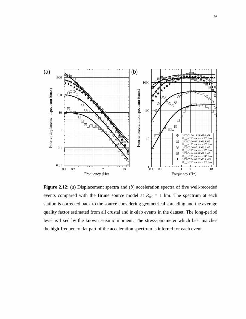
26
Figure 2.12: (a) Displacement spectra and (b) acceleration spectra of five well-recorded
events compared with the Brune source model at Rref = 1 km. The spectrum at each
station is corrected back to the source considering geometrical spreading and the average
quality factor estimated from all crustal and in-slab events in the dataset. The long-period
level is fixed by the known seismic moment. The stress-parameter which best matches
the high-frequency flat part of the acceleration spectrum is inferred for each event.

27
Figure 2.13: The double-bump feature in the spectrum (26 July 2003, 07:13:00) is
persistent across a wide range of distances and azimuths (Az.).

28
Table 2.3: Regression coefficients for the five well-recorded events considering the fixed
geometrical spreading of -1.0 (R ≤ 50 km) and -0.5 (R > 50 km). ∆σ is stress-drop and
Rmax is the hypocentral cut-off distance considered for each event.
2.6 Discussion and Conclusion
The results show, with a very high level of confidence, that attenuation is greater in
the backarc than in the forearc direction, especially at higher frequencies. These results
are summarized in Figure 2.14. After calculating Q-values for each event, the average
and the standard deviation of Q-values at each frequency is calculated for all In-slab and
Crustal events at forearc and backarc regions. The regional quality factor can be
expressed as log10Q(f) = -0.0504log10(f)2 + 1.0096log10(f) + 2.3771 for forearc regions, in
comparison with log10Q(f) = -0.0394log10(f)2 + 0.7888log10(f) + 2.2987 for backarc
regions, considering all in-slab events (depth range from 60 to 150 km). For crustal
events, the quality factor can be described by log10Q(f) = -0.7805log10(f)2 + 1.6918log10(f)
+ 2.1838 for forearc regions and log10Q(f) = -0.3280log10(f)2 + 1.0714log10(f) + 2.0668

29
for backarc regions. An interesting feature is that the quality factor saturates at high
frequencies for crustal events (∼1000), while it continues to increase with frequency for
in-slab events. Attenuation studies in other regions (Leary and Abercrombie, 1994;
Abercrombie, 1995; Castro et al., 2004) have also found that Q has weak frequency
dependence at high frequencies. Castro et al. (2004) associated the change in frequency
dependence of Q at high frequencies with the presence of faults in the crust. By contrast
with the crustal attenuation, in-slab events show efficient propagation of high-frequency
radiation.
Figure 2.14: Comparison of quality factors for all (a) in-slab events and (b) crustal
events in the dataset. A quadratic polynomial function is fitted to forearc (solid line) and
backarc (dashed line) attenuation results. Symbols are the average values of quality
factors; error bars show standard deviation (±1σ) around the mean.
The apparent efficiency of high-frequency propagation for in-slab events, as
evidenced by the quality factor, increases with focal depth as shown in Figure 2.15.
Furthermore, the greater the depth of the event, the greater is the difference between the
quality factors for forearc and backarc paths.

30
Figure 2.15: Empirical relation between quality factors as a function of focal depth.
Symbols represent Q-values for each event at 10 Hz. The solid line is the best fit for the
forearc region [log10Q(10 Hz) = 0.1827log(h)2 - 0.1894log(h) + 2.8] and the dashed line
is the relation describing the trend of Q versus focal depth for the backarc region
[log10Q(10 Hz) = 0.3303log(h)2 - 0.2342log(h) + 2.8].
A possible mechanism for the difference between the Q-values for forearc and
backarc travel paths, for in-slab events, is the portion of wave propagation path within the
high-Q slab, as shown schematically in Figure 2.1 and supported by the results in Figure
2.15. Deep-focus in-slab events have greater path lengths within the high-Q, high-
velocity slab, for the forearc stations (Zhao, 2010). For crustal and in-slab events
recorded by stations in the backarc region, the decrease in Q value along the wave travel
path may be caused by the hot melted rocks below the volcanoes. For events having a
mixed travel path, it is possible to estimate the additional anelastic attenuation for the
estimated length of the wave path within the low Q volcanic zone (Zhao, 2010).
The dependence of Q on travel path type has implications for seismic hazard analysis.
In probabilistic seismic hazard analysis, generally two types of uncertainty are

31
distinguished: epistemic uncertainty (due to lack of data and knowledge) and aleatory
uncertainty (random variability) (Toro et al., 1997). In ground-motion prediction
equations (GMPEs), the standard deviation of the residuals (where the residual is the
difference between the logarithm of an observation and the logarithm of an estimated
value), denoted by σ, is treated as aleatory variability and integrated across in the hazard
analysis. Sigma has a significant influence on the results of seismic hazard analyses,
particularly for low probabilities (Atkinson and Charlwood, 1983; Restrepo-Vélez and
Bommer, 2003; Bommer and Abrahamson, 2006).
To examine the component of σ associated with the distinction of forearc versus
backarc paths, we calculated the standard deviation of residuals for each event in the
dataset, separately. The separation of forearc and backarc travel paths results in a
significant reduction in the standard deviation (σ) of ground-motion predictions. In
Figure 2.16 the intraevent variability of crustal and in-slab events is shown. The symbols
represent the average value of residuals at each frequency for all the events. It can be
clearly seen from this figure that using separate quality factors for forearc/backarc
regions reduces σ, particularly for in-slab events at higher-frequencies, which are most
greatly affected by the heterogeneous attenuation structures of subduction zones. It is also
noted that the intraevent variability is greater at high frequencies for in-slab events, in
comparison with that for crustal events. This may be because the apparent in-slab
attenuation at high frequencies depends on focal depth (Figure 2.15), so that the mixing
of focal depths within the in-slab database leads to increased variability.

32
Figure 2.2.16: Illustration of reduction of intraevent variability in (a) crustal events and
(b) in-slab event by considering separate quality factors for forearc and backarc regions.
The symbols are the mean value of σ for the two cases. The open horizontal squares are
average residuals at each frequency considering a single quality factor. The filled black
vertical squares are the average residuals using separate forearc and backarc anelastic
attenuation terms.

33
2.7 References
Abercrombie, R. (1995), Earthquake source scaling relationships from -1 to 5 ML using
seismograms recorded at 2.5 km depth, J. Geophys. Res., 100, 24,015-24,036.
Aki, K. (1980). Attenuation of shear waves in the lithosphere for frequencies from 0.05 to
25 Hz, Phys. Earth Planet. Inter., 21, 50-60.
Atkinson, G. M. (2004). Empirical attenuation of ground motion spectral amplitudes in
southeastern Canada and the northeastern United States, Bull. Seism. Soc. Am. 94,
1079–1095.
Atkinson G. M. and R. G. Charlwood (1983). Uncertainties in probabilistic seismic
hazard assessment as a function of probability level: A case history for
Vancouver, British Columbia. Bull. Seism. Soc. Am., 73, 1225 - 1241.
Atkinson, G. M. and S. Chen (1997). Regional seismograms from historical earthquakes
in southeastern Canada. Seism. Res. L., 68, 797-807.
Atkinson, G. M. and R. Mereu (1992). The shape of ground motion attenuation curves in
Southeastern Canada, Bull. Seism. Soc. Am. 82, 2014-2031.
Bay, F., D. Fah, L. Malagnini, and D. Giardini (2003). Spectral shear-wave ground
motion scaling in Switzerland, Bull. Seism. Soc. Am. 93, 414–429.
Boatwright, J. (1994). Regional propagation characteristics and source parameters of
earthquakes in eastern North America, Bull. Seism. Soc. Am. 84, 1–15.
Bommer J. J. and N. A. Abrahamson (2006). Why do modern probabilistic seismic-
hazard analyses often lead to increased hazard estimates? Bull. Seism. Soc. Am.
96, 1967 - 1977.
Boore, D. (2003). Simulation of ground motion using the stochastic method, Pure Appl.
Geophys. 160, 636–676.
Boore, D. (2004). Estimating 30sV (or NEHRP site classes) from shallow velocity
models (depths <30 m), Bull. Seism. Soc. Am. 94, 591-597.
Boore, D. M., A. Skarlatoudis, B. Margaris, C. Papazachos, and C. Ventouzi, (2009).
Along-arc and backarc attenuation, site response, and source spectrum for the
intermediate-depth 8 January 2006 M 6.7 Kythera, Greece, earthquake, Bull.
Seism. Soc. Am. 99, 2410-2434.
Boore, D. (1983). Stochastic simulation of high-frequency ground motions based on
seismological models of the radiated spectra, Bull. Seism. Soc. Am. 73, 1865-
1894.
Brune, J. N. (1970). Tectonic stress and the spectra of seismic shear waves from
earthquakes, J. Geophys. Res. 75, 4997-5009.
Brune, J. N. (1971). Tectonic stress and the spectra of seismic shear waves from
earthquakes: correction, J. Geophys. Res. 76, 5002.

34
Burger, R., P. Somerville, J. Barker, R. Herrmann, and D. Helmberger (1987). The effect
of crustal structure on strong ground motion attenuation relations in eastern North
America, Bull. Seism. Soc. Am. 77, 420–439.
Campbell, K. (1991). An empirical analysis of peak horizontal acceleration for the Loma
Prieta, California, earthquake of 18 October, 1989, Bull. Seism. Soc. Am. 81,
1838-1858.
Castro, R. R., F. Pacor, A. Sala and C. Petrungaro (1996). S-wave attenuation and site
effects in the region of Friuli, Italy, J. Geophys. Res. 101, 22355-22369.
Castro, R.R., Gallipoli, M.R. and Mucciarelli, M. (2004). An attenuation study in
southern Italy using local and regional earthquakes recorded by the seismic
network of Basilicata, Ann. Geophysics, 47, 1597-1608.
Chun, K.-Y., G. F. West, R. J. Kokoski, and C. Samson (1987). A novel technique for
measuring Lg attenuation—results from eastern Canada between 1 to 10 Hz, Bull.
Seism. Soc. Am.77 ,398 –419.
Converse, A. M., and A. G. Brady (1992). BAP: basic strong-motion accelerogram
processing software, version 1.0, U.S. Geol. Surv. Open-File Rept. 92-296A, 174
Cormier, V. (1982). The effect of attenuation on seismic body waves, Bull. Seism. Soc.
Am. 72, S169–S200.
Dhakal Y. P., N. Takai, and T. Sasatani (2008). Path effects on prediction equations of
pseudo-response spectra in northern Japan, The 14th
World Conference on
Earthquake Engineering, October 12-17, 2008, Beijing, China
Eurocode 8 (2004). Design of structures for earthquake resistance, part 1: General rules,
seismic actions and rules for buildings, EN 1998-1, European Committee for
Standardization (CEN), http://www.cen.eu/cenorm/homepage.htm.
Frankel, A., D. Carver, E. Cranswick, M. Meremonte, T. Bice, and D. Overturf (1999).
Site responses for Seattle and source parameters of earthquakes in the Puget
Sound region, Bull. Seism. Soc. Am. 89, 468–483.
Frankel, A., A. McGarr, J. Bicknell, J. Mori, L. Seeber, and E. Cranswick (1990).
Attenuation of high-frequency shear waves in the crust: measurements from New
York State, South Africa, and southern California, J. Geophys. Res. 95(B11),
17,441–17,457.
Fukushima, Y., C. Berge-Thierry, P. Volant, D. Griot-Pommera, and F. Cotton (2003).
Attenuation relation for West Eurasia determined with recent near-fault records
from California, Japan and Turkey, J. Earthquake Eng. 7, 573-598.
Hasegawa, A., S. Horiuchi, and N. Umino (1994). Seismic structure of the northeastern
Japan convergent margin: A synthesis, J. Geophys. Res., 99, 22295–22311
Hasegawa, A., N. Umino, and A. Takagi (1985). Seismicity in the northeastern Japan arc
and seismicity patterns before large earthquakes, Earthquake Predict. Res., 3,
607-626

35
Hatzidimitriou, P. M. (1995). S-wave attenuation in the crust in northern Greece, Bull.
Seism. Soc. Am. 85, 1381–1387.
Kanno, T., Narita, A., Morikawa, N., Fujiwara, H. and Fukushima, Y. (2006). A new
attenuation relation for strong ground motion in Japan based on recorded data.
Bull. Seism. Soc. Am. 96, 879-897.
Kobayashi, S., Takahashi, T., Matruzaki, S., Mori, M., Fukushima, Y., Zhao, J.X. and
Somerville, P.G. (2000), A spectral attenuation model for Japan using digital
strong motion records of JMA87 type, 12th
World Conference of Earthquake
Engineering, 2000, Auckland, New Zealand.
Leary, P.C. and Abercrombie, R.E. (1994), Frequency-dependent crustal scattering and
absorption at 5-160 Hz from coda decay observed at 2.5 km depth, Geophys. Res.
Lett. 21, 971-974.
Morikawa N., Kanno, T., Narita A., Fujiwara, H. and Fukushima, Y. (2006). New
additional correction terms for attenuation relations of peak amplitudes and
response spectra corresponding to the anomalous seismic intensity in northeastern
Japan. Journal of Japan Association of Earthquake Engineering 6, 23-40 (in
Japanese with English abstract).
Macias, M., G. M. Atkinson, and D. Motazedian (2008). Ground motion Attenuation,
Source, and Site Effects for the 26 September 2003 M 8.1 Tokachi-Oki
Earthquake Sequence, Bull. Seism. Soc. Am. 98, 1947–1963.
NBCC (2005) National Building Code of Canada. National Research Council of Canada,
Ottawa, NRCC 47666.
NEHRP (2000). NEHRP Recommended provisions for seismic regulations for new
buildings and other structures, Part 1, Provisions, FEMA 368, Washington, D. C.:
Federal Emergency Management Agency.
Ordaz, M., and S. K. Singh (1992). Source spectra and spectral attenuation of seismic
waves from Mexican earthquakes, and evidence of amplification in the hill zone
of Mexico City, Bull. Seism. Soc. Am. 82, 24-43.
Pezzo, E. D., J. Ibanez, J. Morales, A. Akinci, and R. Maresca (1995). Measurements of
intrinsic and scattering seismic attenuation in the crust, Bull. Seism. Soc. Am. 85,
1373–1380.
Rautian, T. G. and Khalturin, V. I. (1978). The use of the coda for determination of the
earthquake source spectrum. Bull. Seism. Soc. Am. 68, 923-948.
Restrepo-Velez, L.F. and Bommer, J.J. (2003) An exploration of the nature of the scatter
in ground motion prediction equations and the implications for seismic hazard
assessment, Journal of Earthquake Engineering, 7 (Special Issue 1), 171-199.
Scherbaum, F. (1994). Basic Concepts in Digital Signal Processing for Seismologists,
Springer-Verlag, Berlin, 158 pp.
Shin, T.-C. and R. B. Herrmann (1987). Lg attenuation and source studies using 1982
Mirimichi data, Bull. Seism. Soc. Am. 77, 384-397.

36
Somerville, P. and J. Yoshimura (1990). The influence of critical Moho reflections on
strong ground motions recorded in San Francisco and Oakland during the 1989
Loma Prieta earthquake, Geophys. Res. Lett. 17, 1203-1206.
Somerville, P.G., J.P. McLaren, C.K. Saikia, and D.V. Helmberger (1990). The
November 25, 1988 Saguenay, Quebec earthquake: source parameters and the
attenuation of strong ground motion. Bull. Seism. Soc. Am., 80, 1118-1143.
Somerville, P., N. Collins, N. Abrahamson, R. Graves, and C. Saikia (2001). Earthquake
source scaling and ground motion attenuation relations for the central and eastern
United States. U.S. Geological Survey Final Report Award No. 99HQGR0098.
Strasser, F. O., and J. J. Bommer (2005). Analysis of intra-event ground motion residuals
from K-NET and KiK-NET data, Department of Civil and Environmental
Engineering, Geotechnics Section, Research report 05-003-SM, Imperial College,
London.
Sugimura, A. (1960). Zonal arrangement of some geophysical and petrological features in
Japan and its environs, J. Fac. Sci. Univ. Tokyo (Sect. 2) 12, 133–153.
Toro, G., N. Abrahamson, and J. Schneider (1997). Model of strong ground motions from
earthquake in central and eastern North America: best estimates and uncertainties,
Seism. Res. Lett. 68, 41–57.
Trifunac, M. D. (1976). Preliminary empirical model for scaling Fourier amplitude
spectra of strong ground acceleration in terms of earthquake magnitude, source-
to-station distance, and recording site conditions. Bull. Seism. Soc. Am. 66, 1343-
1373.
Yoshimoto, K., Wegler, U. and Korn, M. (2006). A volcanic front as a boundary of
seismic attenuation structures in northeastern Honshu, Japan. Bull. Seism. Soc.
Am. 96, 637-646.
Zhao J. X (2010). Geometric spreading functions and modeling of volcanic zones for
strong-motion attenuation models derived from records in Japan, Bull. Seism. Soc.
Am. 100, 721–732.
Zhao J. X., J. Zhang, A. Asano, Y. Ohno, T. Oouchi, T. Takahashi, H. Ogawa, K. Irikura,
H. K. Thio, P. G. Somerville, Y. Fukushima, and Y. Fukushima (2006).
Attenuation relations of strong ground motion in Japan using site classification
based on predominant period, Bull. Seism. Soc. Am. 96, 898–913.

37
Chapter 3
"It is an easy matter to select two stations within 1,000 feet of
each other where the average range of horizontal motion at the
one station shall be five times, and even ten times, greater than
it is at the other” John Milne, (1898, Seismology)
3 Implications of the 2011 M9.0 Tohoku Japan Earthquake for
the Treatment of Site Effects in Large Earthquakes2
3.1 Introduction
Site amplification, or the increase in amplitudes of seismic waves as they traverse soft
soil layers near the Earth’s surface, is a major factor influencing the extent of earthquake
damage to structures (Borcherdt 1970; Nakamura 1989; Lermo and Ch´avez-Garc´ıa
1994; Field and Jacob 1995). Thus an understanding of site-specific amplification effects
and their role in determining ground motions is important for the design of engineered
structures. The methods utilized for site effect analysis from recorded motions can be
divided into three general approaches. A classical method of estimating site response, the
standard spectral ratio (SSR) approach, has been to determine the ratio of the motions
recorded on a soil site to those recorded on a nearby reference rock site (e.g., Borcherdt,
1970; Hartzell, 1992; Field and Jacob, 1995; Kato et al. 1995; Field, 1996; Hartzell et al.
1996; Su et al. 1996; Bonilla et al. 1997). In this method, it is assumed that the reference
rock site does not amplify ground motion. However, it is difficult to find a true reference
site due to the prevalence of a weathered layer near the surface everywhere (Steidl et al.
2 A version of this chapter has been submitted for publication. Ghofrani H., G. M. Atkinson, and K. Goda
(2012). “Implications of the 2011 M9.0 Tohoku Japan Earthquake for the Treatment of Site Effects in
Large Earthquakes,” Bulletin of Earthquake Engineering

38
1996); the reference rock site may also have significant amplification due to impedance
effects associated with its shear-wave velocity gradient. Moreover, if the reference rock
site is not very close to the soil site, then the incident wave field may not have the same
characteristics. Other variants of the spectral ratio approach include the use of cross-
spectral ratios (Safak, 1991; Steidl, 1993), response spectral ratios (e.g., Kitagawa et al.
1992), ratios of peak, RMS (root-mean-square), or effective accelerations (e.g., Borcherdt
and Wenworth, 1995), and blind deconvolution techniques (Zerva et al., 1995).
The second method uses generalized inversion techniques to characterize site
amplification. In this method, the source, path, and site characteristics are identified
simultaneously (e.g., Andrews, 1986; Boatwright et al., 1991; Hartzell, 1992); reviews of
this method can be found in Bard (1994) and Field and Jacob (1995). The advantage of
this method is that it provides the absolute amplification/de-amplification of body waves
(S-wave) at a site. However, like the SSR technique, the generalized inversion method
also suffers from the need to define a reference site.
The third common method of quantifying the site effects is known as the single-station
method (Langston, 1979; Nakamura, 1989). This technique is based on the horizontal-to-
vertical spectral ratio of the motions at a site, which makes it convenient in cases where
no reference site is available. Reviews of this method can be found in Lachet and Bard
(1994), Field and Jacob (1995), and Atakan (1995).
In this study, we are able to use a more direct variant of the SSR approach, in which
the reference site is at the bottom of a borehole, directly below the soil site. Borehole data
are very useful in measuring site effects. For example, borehole measurements have
provided direct in situ evidence of nonlinearity (e.g., Seed and Idriss, 1970; Wen et al.,
1994; Zeghal and Elgamal, 1994; Iai et al., 1995; Sato et al., 1996; Aguirre and Irikura,
1997; Satoh et al., 2001a); for surface-rock recordings they can be used as input motion
to soil columns (e.g. Satoh et al., 1995; Steidl et al., 1996; Boore and Joyner, 1997), and
they have provided information about scaling of earthquakes of different magnitudes
(e.g., Kinoshita, 1992; Abercrombie, 1997). The problems associated with using borehole
data as the input to a site transfer function were discussed by Cadet et al. (2011). The

39
most significant effect is the interference between the incident wave and the reflection
from the surface and any other velocity contrasts (discontinuities) in the soil column. The
destructive interference of the incident wave field and the downgoing waves may produce
holes in the ground-motion spectral ratio (Steidl et al., 1996). Consequently, a direct
spectral ratio between the surface and the total motion at depth generally produces
pseudo-resonances where these holes are present. These phenomena are referred to as the
depth effect (Cadet et al., 2011). These effects should be taken into account when using
surface-to-borehole spectral ratios (S/B) for computing the transfer function of a site.
Site amplification effects were profound for the 2011 M9.0 Tohoku event. As an
illustration, Figure 3.1 compares surface and borehole ground motions at station
MYGH04 (The location of this station relative to the fault plane is indicated by a black
square in Figure 3.2). Amplitudes of ground motions at the borehole level (~0.1g) are
amplified by a factor of 5 at the surface; this large amplification is due to the presence of
a shallow low-velocity layer, about 4 m thick, that overlies stiff bedrock.

40
Figure 3.1: Comparison of observed surface and borehole ground motions for MYGH04
station of the KiK-NET. The values at the end of each trace list the peak ground
acceleration in cm/s2 for East-West (EW), North-South (NS), and Vertical (UD)
components, respectively. All the records are plotted on the same scale. Time series in
black are recorded on the surface, and those in green are recorded in the borehole. The
plot on the right is the shear-wave velocity profile of the corresponding site. The site is at
~91 km from the fault plane and categorized as NEHRP site class C (very dense soil and
soft rock), with VS30 = 850 m/s. The seismometer is installed at a depth of 100 m at this
station.

41
Figure 3.2: The spatial distribution of all KiK-NET stations (black dots) and those
stations recorded the Tohoku event (green dots). The star is the epicenter. The major
tectonic boundaries – the trench and the volcanic front – are represented by dashed black
and red lines, respectively. A blue rectangle shows the fault plane obtained from the GPS
Earth Observation Network System (GEONET) data analysis (http://www.gsi.go.jp/)
In this study, we perform a thorough analysis of site amplification during the Tohoku
event (as well as other Japanese events of M > 5.5). We take advantage of the vertical
array of KiK-NET (KIBAN kyoshin network: http://www.kik.bosai.go.jp/) including the
enriched database of NIED (National Research Institute for Earth Science and Disaster
Prevention: http://www.bosai.go.jp/e/) to estimate the site transfer functions for all sites,
considering both linear and nonlinear site effects. The applicability of the horizontal-to-

42
vertical (H/V) spectral ratio technique as an alternative tool to estimate site response is
evaluated by modeling the relationship between H/V ratios and S/B ratios, as a function
of physical site properties. We develop a suite of simple, useful, and reliable models for
prediction of site amplification effects based on readily-obtainable site parameters.
Finally, we develop an empirical model of ground motions for the Tohoku earthquake
(including site effects) and compare it to the predictions of several existing ground
motion prediction equations (GMPEs) commonly used in seismic hazard analysis
applications.
3.2 Strong ground motion data and record processing
The strong-motion data used in this study were collected from the KiK-NET network of
the National Research Institute for Earth Science and Disaster Prevention (NIED) of
Japan. KiK-NET consists of 687 strong-motion observation stations installed both on the
ground surface and at the bottom of boreholes (directly below the surface site). Figure 3.2
shows the distribution of KiK-NET stations triggered by the Tohoku event.
To enable a statistically-robust and meaningful analysis of site effects, we supplement
the Tohoku-event data by adding all other events of M ≥ 5.5 that were recorded on all
KiK-NET stations from 1998 to 2009. For 687 KiK-NET stations, we have processed and
analyzed 30,453 records from 258 earthquakes in total. The number of events for each
station varies from 4 to 150. The processing procedure for all records includes
windowing, correction for baseline trends and band-pass filtering. We have applied non-
causal, band-pass Butterworth filters with an order of 4. The selected frequency range of
analysis is 0.1 to 15 Hz. The lower frequency limit was selected by inspecting many
records, and concluding that this value is appropriate to produce well-shaped
displacement time series, with a flat portion of the displacement spectrum at low
frequencies. The upper limit is chosen by considering the cut-off frequency of the
seismograph response spectrum (15 Hz). For each record, we compute the instrument-
corrected Fourier amplitude spectrum of acceleration (FAS).

43
3.3 Calculation of site response using surface-to-borehole
spectral ratio (S/B)
Surface-to-borehole spectral ratios (S/B) are used to provide a direct measure of site
response. However, destructive interference between the up-going incident wave field
and down-going reflected waves from the surface at specific frequencies can produce a
notch in the FAS of the borehole recording (Shearer and Orcutt, 1987; Steidl et al., 1996).
The existence of this hole in the borehole spectrum could produce peaks in the spectral
ratios that could be misinterpreted as site-response peaks. Figure 3.3 schematically
illustrates the problem. In this figure, the amplitude spectrum of incident waves is
denoted “A”, while that of the reflections is denoted “B”. It is assumed that the soil
profile consists of n layers overlying bedrock. As the incident and reflected waves always
constructively interfere at the surface, the total amplitude for the outcrop rock would be
2An, while for the station over the soil column it would be 2A1. The ratio of motions
recorded at the surface on soil to those on bedrock can be defined as:
nn BA
A
B
S
12
, (3.1)
The factor two in the numerator represents the free-surface amplification. At the
borehole level, the downgoing reflected waves are interfering destructively and will
reduce the apparent amplitude of the incident waves, thus obscuring the actual site
response.

44
Figure 3.3: Schematic representation of site amplification. Soil profile consists of n
layers where incident and reflected waves for each layer are denoted as Ai and Bi (i = 1 to
n), respectively. Amplification can be defined as the surface-to-borehole (S/B) spectral
ratio (Equation 3.1) or surface-to-outcrop (standard) spectral ratio (SSR: 2A1/2An)
A possible solution to the destructive interference problem involves the use of cross-
spectrum techniques (Bendat and Piersol, 2006; Safak, 1991; Field et al., 1992; Steidl,
1993), which consider the coherency of the waveforms at the surface and down-hole.
Taking into account the effect of the reflected wave-field, S/B ratios are multiplied by the
coherence (C2) between surface and borehole recordings (following Steidl et al., 1996).
The coherence is defined as:
fSfS
fSC
2211
2
122 , (3.2)
and thus the depth-corrected cross spectral ratios are given by:
BSCBS 2'/ , (3.3)
where S11(f) and S22(f) are the power spectral densities of the seismograms recorded at
the surface and downhole, respectively, S12(f) is the cross-power-spectral density function
(Steidl et al., 1996), and S/B’ is the S/B ratio corrected for the depth effect. It should be
mentioned that a loss in coherence could be due to the site response itself, and not solely
to the destructive interference effect.

45
Another possible way to correct the S/B ratio for the depth effect is to use empirical
correction factors as proposed recently by Cadet et al., (2011). The key parameter in their
correction factors is the fundamental resonance frequency (f0) of a site. In their paper, the
fundamental resonance frequency was defined as the frequency corresponding to the first
(i.e., lowest frequency) peak of the S/B ratio. A “peak” is defined as a specific local
maximum with amplitude larger than 2 in a statistical sense (Cadet et al., 2011). Knowing
the average shear wave velocity (VS) over the depth of the borehole (Db), the so-called
first destructive interference frequency (fd1) of the soil column can also be estimated
using fd1 = Vs/4Db.
To illustrate the issues, Figure 3.4 shows recorded FAS and S/B ratios for two
representative sites (ABSH10 and AICH12). Based on the definition of resonance
frequency (f0) given by Cadet et al. (2011) (i.e. the lowest frequency peak with amplitude
> 2.0), we might choose f0 ~2.0 Hz for both stations. Referring to Figure 3.4, we can see
that the increase in the amplitude of S/B for ABSH10 near 2.0 Hz is due to a
corresponding drop of FAS at the borehole level because of downward reflections.
However, the significant amplification at the surface in AICH12 near 2.0 Hz is clearly
due to actual site amplification; it is not due to interference of incident and reflected
waves at the borehole, and should therefore not be reduced using correction factors. We
found that, in general, empirical correction factors and cross-spectral ratio techniques
produced similar results in terms of eliminating depth effects. However, we prefer the
cross-spectral ratio techniques as it is easier to apply and less subject to
misinterpretations due to problems, such as that illustrated in Figure 3.4. We therefore
used the cross-spectral ratio techniques to calculate S/B’ as defined by Equation 3.3.

46
Figure 3.4: Comparing the amplification functions at two different stations. The top row
is showing S/B ratio (horizontal component) for the Tohoku event data (green line) along
with the corresponding average for all KiK-NET data (solid black line), and its 1σ
bounds (shaded gray). The bottom row plots the FAS of horizontal components
(geomean) for Tohoku, for both surface and borehole ground motions. The solid lines are
the smoothed spectra.
We performed some checks as to how the amplifications derived using S/B’ ratios
compare to those computed theoretically. In order to estimate the theoretical site response
we use the RATTLE program (C. Mueller, U. S. Geological Survey), which calculates
the one-dimensional (1D) transfer function of a layered, damped soil over an elastic

47
bedrock, for a vertically propagating shear-wave (SH), using Haskell's approach (Haskell,
1960). The input data for RATTLE are the layered velocity model, specifying the
thickness, density, shear-wave velocity, and Q factor for each layer. For density and Q
factor we used values as reported by Cadet et al. (2011). The other input parameters are
the velocity and density of the half-space, incident angle, and the depth with respect to
which the transfer function is calculated. This reference depth is just the depth of
installation for borehole sensors. We compared the fundamental frequencies and
amplitude of amplification as obtained from the theoretical transfer function with the
corresponding values as deduced from the S/B’ ratios (after correction for depth effects),
for 167 sites for which there is a clear, statistically-significant single peak in their H/V
ratio. We found close agreement between the theoretical transfer functions and
observations, in agreement with similar results from other studies (Steidl et al., 1996;
Cadet et al., 2011). Observed and predicted fundamental frequencies are strongly
correlated (correlation coefficient of 0.95), with standard deviation of residuals (empirical
S/B’ – theoretical S/B’) of σresidual = 0.08 (log base 10). The agreement between S/B’ and
theoretical amplification amplitude is not as close as that for the fundamental frequencies,
with a mean residual of almost zero and σresidual = 0.23. The mismatch between observed
and theoretical site response amplitudes could be the result of errors in the parameters
specifying the velocity profiles, densities and Q factors used for computing the transfer
functions. Figure 3.5 shows some examples of the RATTLE computations comparing to
the theoretical transfer function for SH-waves (Kramer, 1996), and S/B’ ratios.

48

49
Figure 3.5: Comparing the RATTLE computations (red) with the theoretical transfer
function for SH-waves (surface/borehole in green and surface/outcrop in purple), and
S/B’ ratios (black) at three representative KiK-NET stations. The grey jagged line in the
background is H-S/H-B before smoothing.
3.4 Relationship between amplification and site parameters
3.4.1 Linear site amplification
In this section, we examine the relationship between site amplification (as given by S/B’
ratios) and site variables describing the depth and stiffness of the deposit. As a
commonly-used index parameter for the shear-wave velocity profile, we use the average
shear-wave velocity in the uppermost 30 m (Borcherdt, 1992; 1994):
N
i i
iS
v
dV
1
30 30 , (3.4)
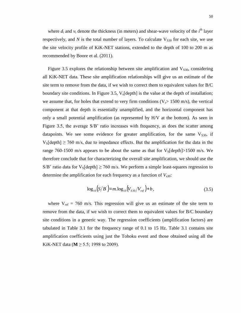
50
where di and vi denote the thickness (in meters) and shear-wave velocity of the ith
layer
respectively, and N is the total number of layers. To calculate VS30 for each site, we use
the site velocity profile of KiK-NET stations, extended to the depth of 100 to 200 m as
recommended by Boore et al. (2011).
Figure 3.5 explores the relationship between site amplification and VS30, considering
all KiK-NET data. These site amplification relationships will give us an estimate of the
site term to remove from the data, if we wish to correct them to equivalent values for B/C
boundary site conditions. In Figure 3.5, Vs[depth] is the value at the depth of installation;
we assume that, for holes that extend to very firm conditions (Vs> 1500 m/s), the vertical
component at that depth is essentially unamplified, and the horizontal component has
only a small potential amplification (as represented by H/V at the bottom). As seen in
Figure 3.5, the average S/B’ ratio increases with frequency, as does the scatter among
datapoints. We see some evidence for greater amplification, for the same VS30, if
VS[depth] ≥ 760 m/s, due to impedance effects. But the amplification for the data in the
range 760-1500 m/s appears to be about the same as that for VS[depth]>1500 m/s. We
therefore conclude that for characterizing the overall site amplification, we should use the
S/B’ ratio data for VS[depth] ≥ 760 m/s. We perform a simple least-squares regression to
determine the amplification for each frequency as a function of Vs30:
bVVmBS refS 3010
'
10 log.log , (3.5)
where Vref = 760 m/s. This regression will give us an estimate of the site term to
remove from the data, if we wish to correct them to equivalent values for B/C boundary
site conditions in a generic way. The regression coefficients (amplification factors) are
tabulated in Table 3.1 for the frequency range of 0.1 to 15 Hz. Table 3.1 contains site
amplification coefficients using just the Tohoku event and those obtained using all the
KiK-NET data (M ≥ 5.5; 1998 to 2009).
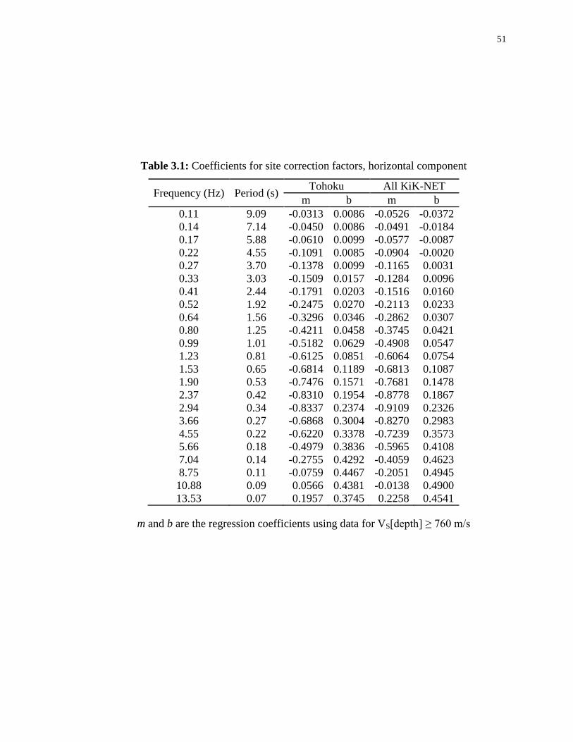
51
Table 3.1: Coefficients for site correction factors, horizontal component
Frequency (Hz) Period (s) Tohoku All KiK-NET
m b m b
0.11 9.09 -0.0313 0.0086 -0.0526 -0.0372
0.14 7.14 -0.0450 0.0086 -0.0491 -0.0184
0.17 5.88 -0.0610 0.0099 -0.0577 -0.0087
0.22 4.55 -0.1091 0.0085 -0.0904 -0.0020
0.27 3.70 -0.1378 0.0099 -0.1165 0.0031
0.33 3.03 -0.1509 0.0157 -0.1284 0.0096
0.41 2.44 -0.1791 0.0203 -0.1516 0.0160
0.52 1.92 -0.2475 0.0270 -0.2113 0.0233
0.64 1.56 -0.3296 0.0346 -0.2862 0.0307
0.80 1.25 -0.4211 0.0458 -0.3745 0.0421
0.99 1.01 -0.5182 0.0629 -0.4908 0.0547
1.23 0.81 -0.6125 0.0851 -0.6064 0.0754
1.53 0.65 -0.6814 0.1189 -0.6813 0.1087
1.90 0.53 -0.7476 0.1571 -0.7681 0.1478
2.37 0.42 -0.8310 0.1954 -0.8778 0.1867
2.94 0.34 -0.8337 0.2374 -0.9109 0.2326
3.66 0.27 -0.6868 0.3004 -0.8270 0.2983
4.55 0.22 -0.6220 0.3378 -0.7239 0.3573
5.66 0.18 -0.4979 0.3836 -0.5965 0.4108
7.04 0.14 -0.2755 0.4292 -0.4059 0.4623
8.75 0.11 -0.0759 0.4467 -0.2051 0.4945
10.88 0.09 0.0566 0.4381 -0.0138 0.4900
13.53 0.07 0.1957 0.3745 0.2258 0.4541
m and b are the regression coefficients using data for VS[depth] ≥ 760 m/s

52
Figure 3.6: Amplification S/B’ (horizontal components) for the KiK-NET stations
relative to VS30, using all events from 1998 to 2009. Sites are categorized into four groups
based on their VS[depth] which is shear wave velocity at the depth of installation. The
amplification of the vertical component S/B’(vert) is also plotted versus VS30.
Another important site parameter, in addition to site stiffness, is the fundamental
resonance frequency. The fundamental frequency depends on both layer depth and its
stiffness. The mapping of predominant frequency of amplification facilitates the
characterization of risk in seismic-prone areas (Lachet and Bard, 1994). Furthermore,
fundamental frequency may carry information on the deeper part of the soil column, in
comparison to VS30 which considers only the top 30 m. The fundamental frequency is
obtained for the KiK-NET data using the peak of the horizontal-to-vertical (H/V) spectral
ratios of the recorded strong motions at the sites (Lermo and Chávez-García, 1993;
Theodulidis and Bard, 1995; Zhao et al., 2006a; Fukushima et al., 2007), considering all

53
events of M ≥ 5.5 recorded at each station from 1998 to 2009. Only those stations that
recorded at least three events are considered. The peak of the H/V ratio may be
ambiguous as an indicator of fundamental frequency in the case of close proximity to
sources or in the absence of a marked impedance contrast at some depth. However, when
averaged over multiple events, the H/V peak provides a stable estimate of fundamental
frequency that is well-correlated with that obtained from the peak of the S/B’ ratio.
Considering all events recorded at each station, we have calculated the mean value of
horizontal-to-vertical spectral ratios at both surface H/V[surface] and at the bottom of the
borehole H/V[depth]. The latter is helpful in detecting the possible presence of a large
impedance contrast at deeper sections of the borehole. To determine the H/V ratios the
following procedure was applied:
1) Apply a 5% cosine taper function to the signal window;
2) Calculate Fourier amplitude spectra (FAS) of the three components (NS, EW,
UD), for both surface and borehole ground-motions;
3) Smooth the FASs using a Konno-Ohmachi window with bandwidth parameter of
20 (Konno and Ohmachi, 1998)
4) Obtain the geometric mean of the two horizontal components
((FASEWFASNS)0.5
);
5) Calculate the ratio of FAS(H) to FAS(V) at the surface and the borehole
(H/V[surface] and H/V[depth]).
Despite varying amplitudes and predominant frequencies, the H/V[surface] ratios can
be grouped based on their overall shape. About 60% of the stations show a single clear
H/V “peak” which is associated with the fundamental frequency of the site; a peak is
defined as a local maximum where the amplitude is greater than twice the mean level of
H/V[surface]. The rest of the spectral ratios can be divided into groups having two peaks
(20%), more than two peaks (jagged shape), or no significant peak.
At the bottom of the borehole, we would expect H/V[depth] to be unity, if this is at
bedrock level (Nakamura, 1989; Theodulidis et al., 1996). However, for the KiK-NET
stations the borehole sensor in not always placed at bedrock. By inspection of H/V[depth]

54
compared to H/V[surface], there are often peaks at very low-frequencies, which could be
due to significant velocity contrast beneath the downhole sensor (Cadet et al., 2011)
We would expect the fundamental frequency (f0) to be related to the depth-to-bedrock
(i.e. f0 = VS/4HB (Dobry et al., 2000)). Depth-to-bedrock, defined by the depth of a layer
with VS 760 m/s, or to a significant impedance contrast between surface soil deposits
and material with VS 760 m/s, is obtained for each site from the velocity profile. Figure
3.6 plots the fundamental site frequency as a function of VS30. As VS30 is a common site
parameter in engineering seismology, its relationship with other site parameters is
important and useful. It is interesting that Vs30 is a good proxy to estimate the natural
frequency of a site. Furthermore, the fundamental frequency inferred from the H/V ratios
matches well with that derived from the theoretical relation (f0 = VS /4HB). In Figure 3.6,
the upper limit on site frequency at 10 Hz may be artificial due to the limitations of the
instruments and filtering - we would not be able to see peaks at shorter periods clearly.

55
Figure 3.7: Fundamental site frequency as a function of VS30. Gray squares are
observations for which a clear peak frequency is indicated by the H/V ratio. The green
triangles are fundamental site frequencies calculated using the equation f0 = VS/4HB,
where HB is the known depth-to-bedrock. The blue circles are observed fundamental
frequencies of NGA data. Lines are the best linear fit to f0 as a function of VS30 for each
dataset.
To check if the VS30-f0 correlation is region-specific, or the observed relation may be
valid in other tectonic regions, we use the 2005 Pacific Earthquake Engineering Research
Center (PEER) ground motion database which was developed for the 2008 NGA West
project (http://peer.berkeley.edu/smcat/). The PEER-NGA database is the most complete
source of high-quality ground-motion data compiled from active tectonic regions. The
database consists of 3551 multi-component records from 173 shallow crustal earthquakes
(M4.2-7.9). We calculate the H/V ratios for all sites in the database and pick the
fundamental frequencies, considering just those stations that show a clear single peak and
that recorded at least 3 events. As there are relatively few NGA stations having multiple
56
recordings, the slope of the VS30-f0 relation is less significant (0.64 0.10) than that for
Japan (1.33 0.12). The systematically-lower values of f0 for the NGA data, in
comparison to the Japanese data, can be attributed to deeper bedrock (for the same VS30)
for most regions that comprise the NGA database.
Figure 3.7 plots the fundamental site frequency as a function of depth-to-bedrock,
which is interrelated to VS30. We also show in Figure 3.7 the corresponding relationship
for the PEER-NGA strong motion dataset; for the PEER-NGA data, the “depth to
bedrock” is assumed to be the depth to VS = 1.0 km/s (Z1.0), as it is the closest proxy to
our selected VS760 m/s. The Japan and PEER-NGA data show similar trends, but there is
a higher intercept for the PEER-NGA data, probably because they are referenced to
stiffer, deeper bedrock. We also show the estimated Z1.0 from the velocity profiles of
KiK-NET stations in Figure 3.7. We find that with an approximate adjustment, one can
estimate the Z1.0 in Japan and California by using the VS30 and depth-to-bedrock relation
for Japan.

57
Figure 3.8: Depth-to-bedrock as a function of VS30. Gray squares are the depth to VS760
m/s and purple circles are Z1.0 (depth to VS1000 m/s) from velocity profiles of the KiK-
NET stations. The dotted line is the best fit to the Z1.0 values from the NGA database.
The dashed line is the estimated model for predicting Z1.0 in Japan. Note deeper bedrock
for NGA database.
The correlations for fundamental site frequency (f0) and depth-to-bedrock (HB) with
VS30 can be described for Japan by the following linear regressions:
9066.0log331.1log 30
10010
ref
S
V
Vf , (3.6)
9136.0log729.1log 30
1010
ref
S
BV
VH ,
(3.7)
In Figure 3.8, we examine the factors influencing site amplification, specifically
depth-to-bedrock, and VS30. At low frequencies, as we would expect, the large
wavelengths see (sample) only deep deposits. At higher frequencies, we are sampling

58
more of the near-surface materials. Note that shallow sites are relatively stiff in terms of
VS30, and generally show less amplification (except for shallow soil sites at high
frequency).
Figure 3.9: Corrected site amplifications (horizontal components) versus depth-to-
bedrock, at frequency = 0.34, 1.1, and 3.7 Hz. The symbols are binned into different
groups based on VS30.
We developed empirical relationships between site amplification, depth-to-bedrock
and fundamental site frequency, of the following form:
bfaBS 010
'
10 log.log , (3.8)
dHcBS B 10
'
10 log.log ,
(3.9)
where S/B’ is the corrected S/B for depth effect (horizontal component), HB is the
depth-to-bedrock, and f0 is the fundamental frequency of a site. a, b, c, and d are
regression coefficients. The regression coefficients are summarized in Table 3.2.

59
Table 3.2: Regression coefficients of corrected site amplifications relative to the
fundamental site frequency (a and b) and depth-to-bedrock (c and d), respectively.
Frequency (Hz) Period (s) Fundamental frequency (f0) Depth-to-bedrock (HB)
a b c d
0.11 9.09 -0.0670 0.0157 0.0467 -0.0875
0.14 7.14 -0.0678 0.0329 0.0513 -0.0768
0.17 5.88 -0.0650 0.0418 0.0522 -0.0673
0.22 4.55 -0.0716 0.0584 0.0603 -0.0655
0.27 3.70 -0.0971 0.0860 0.0822 -0.0826
0.33 3.03 -0.1304 0.1188 0.1076 -0.1039
0.41 2.44 -0.1534 0.1464 0.1277 -0.1170
0.52 1.92 -0.1966 0.1936 0.1626 -0.1427
0.64 1.56 -0.2208 0.2272 0.1832 -0.1512
0.80 1.25 -0.2398 0.2652 0.2041 -0.1526
0.99 1.01 -0.2615 0.3142 0.2288 -0.1496
1.23 0.81 -0.2956 0.3827 0.2618 -0.1457
1.53 0.65 -0.3099 0.4472 0.2788 -0.1124
1.90 0.53 -0.3011 0.5065 0.2807 -0.0503
2.37 0.42 -0.2849 0.5747 0.2673 0.0457
2.94 0.34 -0.2534 0.6231 0.2280 0.1655
3.66 0.27 -0.1492 0.6166 0.1316 0.3506
4.55 0.22 -0.0655 0.6160 0.0796 0.4705
5.66 0.18 0.0308 0.5980 0.0120 0.6013
7.04 0.14 0.1411 0.5522 -0.0854 0.7523
8.75 0.11 0.2375 0.4801 -0.1683 0.8493
10.88 0.09 0.2731 0.3997 -0.2032 0.8370
13.53 0.07 0.2666 0.2935 -0.2277 0.7590

60
3.4.1.1 Regional site amplification factors
Figure 3.9 plots the average site amplification factors for sites with VS30 of 180, 360, and
600 m/s, respectively, where the amplifications are derived using the coefficients of
Table 3.1 (all KiK-NET data). We also show our estimate of what a representative site
amplification curve should look like for the reference velocity of 760 m/s. Table 3.3
shows the amplifications that come from the regression of log(H/V[depth]) vs.
log(Vs[depth]), evaluated at Vs = 760 m/s (black line in Figure 3.9).
Figure 3.10: Amplification (S/B’) for different NEHRP site classes (soft soil profile in
solid black; stiff soil profile in red; and very dense soil and soft rock in green). The
estimated amplification for a reference velocity of 760 m/s is shown in black (dashed
line).

61
Table 3.3: Ratio of horizontal to vertical component of ground-motion at depth,
evaluated for the reference B/C boundary site condition (VS[depth] = 760 m/s)
Frequency (Hz) Period (s) H/V[depth] for VS[depth] =760 m/s
[Regional site amplification]
0.11 9.09 1.2867
0.14 7.14 1.3798
0.17 5.88 1.5423
0.22 4.55 1.6225
0.27 3.70 1.5661
0.33 3.03 1.4982
0.41 2.44 1.4688
0.52 1.92 1.3020
0.64 1.56 1.1416
0.80 1.25 1.0644
0.99 1.01 0.9900
1.23 0.81 0.9548
1.53 0.65 1.0047
1.90 0.53 1.0716
2.37 0.42 1.1443
2.94 0.34 1.2378
3.66 0.27 1.3490
4.55 0.22 1.3419
5.66 0.18 1.2740
7.04 0.14 1.1415
8.75 0.11 1.0423
10.88 0.09 0.9765
13.53 0.07 0.9845
62
3.4.1.2 Additional site factor: kappa filter
The attenuation of site amplifications at high frequency, as seen in Figure 3.9, is often
represented by the high-frequency attenuation operator, kappa κ (Anderson and Hough,
1984). This high-frequency decay of ground-motions can be modeled by multiplying the
spectrum by the factor P(f):
ffP exp , (3.10)
where κ is a region-dependent or site-dependent parameter. In general, κ will increase
with distance due to path effects; its zero-distance intercept, sometimes referred to as κ0,
is considered to represent path-independent near-surface attenuation of seismic waves.
After correcting ground motions from the Tohoku mainshock for regional site effects
using the coefficients given in Table 3.1, we performed a simple regression analysis to
estimate the anelastic attenuation factor, assuming a fixed geometrical spreading with
slope of -1 over all distance ranges:
cdeff RcRcFAS 110010 loglog , (3.11)
where 22 10 cdeff RR and Rcd is the closest-distance to the fault plane. Based on FAS
regressions, we evaluated and plotted out the spectral shape on a log-linear plot for a few
values of near-source distances, as shown in Figure 3.10. We infer κ = 0.044 from these
spectral shapes.

63
Figure 3.11: Spectral shapes from initial regression of FAS (Tohoku mainshock) after
site correction in log-linear scale. The shape is consistent for different effective distances
(Reff) of 10, 20, and 50 km. The slope of the fitted lines (dashed lines) for frequencies > 2
Hz provides an estimated κ = 0.044.
3.4.1.3 Using H/V[surface] as an extra parameter to estimate site
amplification function
The horizontal-to-vertical (H/V) spectral ratio has been widely used to provide a
preliminary estimate of site amplification (Kanai and Tanaka, 1961; Nogoshi and
Igarashi, 1971; Nakamura, 1989). H/V ratios on soft soil sites generally exhibit a clear,
stable peak that is correlated with the fundamental resonant frequency (Ohmachi et al.,
1991; Field and Jacob 1993, 1995; Lermo and Chavez-Garcia 1994; Lachet et al., 1996;
Bonnefoy-Claudet et al., 2006). However, H/V typically underestimates the site
amplification factor (Field and Jacob, 1995; Bonilla et al., 1997; Satoh et al., 2001b).

64
Considering these findings, we explore the use of H/V as an amplification function for
the KiK-NET data. This will be useful for other applications where H/V is known but
borehole data are not available to constrain site amplification.
We performed a linear regression using:
301023010110 log.760log.log afaVaY S , (3.12)
in which Y is the ratio of the “true” site amplification (S/B’) to an estimate obtained as
the average of H/V[surface] over many events, and f0 is the fundamental frequency of a
site as measured from its average H/V peak frequency. Figure 3.11 shows the
performance of Equation 3.12 as a predictor of site amplification; Table 3.4 summarizes
the regression coefficients for 23 logarithmically spaced frequencies. By using H/V and
VS30 with Equation 3.12, we obtain an excellent match to the observed site transfer
functions for the whole range of frequencies. Applying this new model, over all KiK-
NET stations, the residuals (log(obs) – log(pred)) of site amplification as a function of
VS30 is plotted in Figure 3.12. Using the combination of f0 as determined from H/V and
VS30 gives near-zero residuals for prediction of site amplification for a wide range of site
classes. The advantage of this method could be significant for assessing the site effects by
using a single station or in an area where a rock reference site cannot be found.

65
Table 3.4: Regression coefficients for predicting site amplification (S/B᾿) using Equation
3.12
Frequency (Hz) Period (s) a1 a2 a3
0.11 9.09 0.148 -0.0430 0.001
0.14 7.14 0.143 -0.0334 -0.015
0.17 5.88 0.155 -0.0314 -0.025
0.22 4.55 0.122 -0.0356 -0.028
0.27 3.70 0.103 -0.0317 -0.029
0.33 3.03 0.093 -0.0377 -0.023
0.41 2.44 0.083 -0.0401 -0.014
0.52 1.92 0.075 -0.0646 0.018
0.64 1.56 0.057 -0.0929 0.051
0.80 1.25 0.044 -0.0862 0.057
0.99 1.01 0.020 -0.0842 0.065
1.23 0.81 -0.012 -0.1122 0.099
1.53 0.65 -0.028 -0.1211 0.131
1.90 0.53 -0.087 -0.1345 0.166
2.37 0.42 -0.180 -0.1287 0.179
2.94 0.34 -0.214 -0.1344 0.208
3.66 0.27 -0.260 -0.1328 0.229
4.55 0.22 -0.358 -0.1445 0.253
5.66 0.18 -0.381 -0.1534 0.284
7.04 0.14 -0.372 -0.1343 0.288
8.75 0.11 -0.323 -0.1053 0.302
10.88 0.09 -0.260 -0.0608 0.312
13.53 0.07 -0.155 -0.0171 0.314

66
Figure 3.12: Comparison of S/B’ ratios using cross-spectral ratios (solid black line) for
sample sites (NGNH11, NGNH14, and NGNH20) with mean H/V ratios (dashed black
line). Transfer functions are overlaid by prediction model using VS30 and f0 as predictor
parameters and adding H/V as an extra parameter (green line).
Figure 3.13: Residuals of predicting corrected observed amplifications at different site
classes (varying VS30) using f0, depth-to-bedrock, and H/V as an extra parameter
(Equation 3.12). Bars are indicating ±1σ around the mean.

67
3.5 Non-linear site amplification
To this point, we have assumed linear soil behavior in assessing average site
amplification. Under weak motions, the stress-strain relationship of soil is linear stress =
G strain, where G is the shear modulus. Under strong shaking, soil shows nonlinear and
hysteretic behavior, with the effective modulus G decreasing at high strain (Beresnev and
Wen, 1996). Since the shear-wave velocity is given by GVs (where ρ is density)
the effective shear-wave velocity decreases as the strain increases. On the other hand,
amplification decreases due to damping (loss of energy) in hysteresis. Overall,
nonlinearity will result in a shift of the resonance frequency to lower values, and the
reduction in amplification, as the amplitude of motions increases (Silva, 1986; Beresnev
and Wen, 1996; Field et al., 1997; Dimitriu et al., 2000).
Figure 3.13 shows the nonlinear behavior of a site subjected to strong seismic shaking
(PGA~ 530 cm/s2) during the Tohoku event. The spectral ratio of the stations (MYGH04
from KiK-NET, with VS30 = 850 m/s) is compared for the strongest part of the signal and
the coda-window, noting that the shaking during the coda is a representative of weak-
motion (Chin and Aki, 1991). We hypothesize that the linear-elastic soil response is
restored after the termination of the strong shaking portion. We have assumed that the
coda window starts at the lapse time later than seven times the S-wave arrival time. If
nonlinear behavior exists, it should appear as a discrepancy in site response
characteristics between weak and strong motions. From Figure 3.13, a clear shift of the
peak amplitude frequency (fundamental frequency) to lower frequencies during the
strong shaking portion of the record can be seen. Also, the amplitudes are reduced for the
S-window spectral ratios in comparison with the coda-window spectral ratios. However,
it should be mentioned that the coda-window does not necessarily behave in a completely
linear fashion. If soil behaves nonlinearly, some residual deformation will remain, and it
takes at least some time to reconsolidate to the original state (Wu et al., 2010). Thus the
coda may also be affected by soil nonlinearity (residual deformation). For Tohoku, at
some sites the dissipation of pore pressure due to ground shaking might have taken a long
time because of the long duration of shaking. Extensive liquefaction effects from Tohoku

68
are hypothesized to be related to the number of cycles that soil underwent during this
event (Bhattacharya et al., 2011).
Figure 3.14: Amplification (S/B) of the East-West (EW) and North-South (NS)
components at MYGH04 for the S-window of the first arrival (tick solid red), S-window
of the second arrivals (dashed light red), and coda-window (blue)
By contrast to the nonlinear behavior noted in Figure 3.13, we observe linear behavior
in Figure 3.14, which shows similar amplification of S- and coda-window for station
TCGH16. The VS30 for this site is 213 m/s and the borehole is at the depth of 112 m, in a
layer with shear-wave velocity 680 m/s. The ground-motions reached PGA of 1197 cm/s2
in the EW component on the surface, and the PGA of the vertical component at the
borehole level is 137 cm/s2; this is above a common threshold level of ~100 cm/s
2 often
cited for nonlinearity (Beresnev and Wen, 1996).

69
Figure 3.15: Amplification (S/B) of the East-West (EW) and North-South (NS)
components at TCGH16 for the S-window (red) and coda-window (blue)
3.5.1 Time-frequency analysis of borehole data to assess nonlinearity
We apply the moving-window method of Sawazaki et al. (2006, 2009) and Wu et al.
(2009, 2011) to detect the PGA threshold of nonlinearity for each station. This technique
uses Welch's periodogram method of spectral estimation. The short-time Fourier
transform (STFT) of a moving window is calculated for both surface and borehole time
series. Then, the spectra are plotted versus evolution time. This way, a decrease of
fundamental frequency and amplitude due to the nonlinear behavior of a site can be
detected within the strong part of the signal, relative to the coda window and background
noise (representing weak motions). A sample application of the technique is depicted in
Figure 3.15.

70
Figure 3.16: Temporal evolution of S/B for the MYGH04 station. The drop of amplitude
and shifting of the fundamental frequency to lower-frequencies during strong shaking can
be seen clearly in this figure.
In our implementation, we used a moving window with a length of 6 s to examine all
Tohoku waveforms recorded by the surface and borehole stations. Successive windows
have 75% overlap (windows are moved forward by 2 s intervals). The employed 6 s
window appears to offer a good balance between temporal resolution and stability (Wu et
al., 2009; 2010). We remove any linear trend and apply a 5% cosine-taper to both ends of
each window, and compute the Fourier amplitude spectrum (FAS) of the two horizontal
components. The spectra is then smoothed using a Konno-Ohmachi window (b = 20).
The spectral ratios (S/B’) are obtained by dividing the geometric mean of horizontal

71
spectra of surface stations by the corresponding spectra of the borehole stations, tabulated
for 50 frequencies logarithmically spaced between 0.1 to 25 Hz. To estimate the
threshold of nonlinear behavior, we plot the S/B’ ratios as a function of sorted PGA
values obtained from each record. PGA values are binned into 100 classes.
Figure 3.16 illustrates the changes of S/B’ relative to the peak ground acceleration for
site MYGH04, which displays nonlinear behavior. Note the reduction in the fundamental
frequency and the amplification with increasing PGA. The threshold for nonlinearity at
this station is ~25 cm/s2. The threshold values for nonlinearity based on PGA[surface]
and PGA[borehole] are estimated and tabulated for 49 KiK-NET stations in the Appendix
2.
Figure 3.17: Spectral ratios versus recorded PGA for MYGH04. The threshold ground
motion for nonlinear behavior is PGA[surface] ~25 cm/s2.

72
To examine the relative degree of nonlinearity during the Tohoku mainshock, in
comparison to that exhibited during smaller earthquakes, we calculate the average
amplification (S/B᾿) at each station over all events (Aref) and the frequency of that peak
(fref).The same procedure is also applied for just the Tohoku mainshock ground motions.
In this case, the maximum amplitude is called AMS and the fundamental frequency is
called fMS. We consider stations that show a clear-single peak (with an amplitude > 2) in
the H/V at the surface (or S/B᾿ ratio). In total, 225 out of 475 stations passed these
criteria and among them only 42 stations showed nonlinear behavior (shifting of the
fundamental frequency to lower frequencies, and a decrease in amplitude, as deduced
from the moving window technique). To quantify the degree of nonlinearity for these 42
stations, we plot the ratio AMS/Aref and fMS/fref as a function of PGAref, where this is the
predicted median PGA by the Tohoku regression Equation 3.13 (derived below), for VS30
= 760 m/s (reference), on Figure 3.17 (values for other sites, not identified as being
nonlinear, as shown in the background). It is interesting that nonlinear effects are seen for
all soil types. Probably this is because the C sites are typically soft shallow soil over rock.
The plots are showing that there is a clear, steady trend of increasing nonlinearity with
increasing PGA. We fit a linear trend line (for the sites showing nonlinearity) and obtain
the significance of slope and intercept for AMS/Aref and fMS/fref ratios. The p-value of the 2-
tailed t-test for the slope (Figure 3.17a) is 0.22, which is significantly different from 0 at
the 95% confidence level. The standard error (SE) on the slope for AMS/Aref is 0.0014. For
the fMS/fref ratio, the p-value of the slope is 0.0048, which means is also significantly
different from 0 (with SE = 9.3e-4).

73
Figure 3.18: Nonlinearity symptoms: decrease in the predominant frequency (fMS/fref)
and/or amplification amplitude (AMS/Aref) as a function of PGAref (predicted PGA for VS30
= 760 [m/s]). NEHRP site classes are shown with different colors ((a) and (b)) and trend
lines are shown as solid black lines. Grey dots in background show values for sites that
did not exhibit nonlinearity symptoms.
In summary, we found some localized nonlinear soil behavior (such as stations
MYGH04 and IBRH18), and the degree of nonlinearity increases with the intensity of
shaking as would be expected (Figure 3.17). However, nonlinearity was not a pervasive
phenomenon during the Tohoku event, with only a small fraction of sites showing
significant changes in amplification and its peak frequency. On the other hand, it should
be mentioned that there are many cases of liquefaction-related damage during the Tohoku
earthquake, which is clearly evidence of nonlinearity, and that some nonlinearity was also
observed at K-NET sites (Tokimatsu et al., 2011).
3.6 Overall characteristics of Tohoku ground motions
Having evaluated site amplification for the Tohoku motions, we can now examine what
the underlying motions would be without these effects. We fit the Tohoku motions to:
cdcdfactoreff RBcRFccsiteRY ....loglog 2101010 , (3.13)

74
where 22 10 cdeff RR and Rcd is the closest distance to the fault rupture surface. For
stations in the forearc region, F = 1 and B = 0, otherwise (for backarc stations) F = 0 and
B = 1 (Ghofrani and Atkinson, 2011). The sitefactor is m.log(VS30/Vref) + b using
coefficients in Table 3.1. The regression coefficients are given for both FAS and pseudo-
spectral acceleration (PSA) in Table 3.5.
Table 3.5: Regression coefficients for FAS and PSA (geometric mean of horizontal
components)
FAS (cm/s) PSA (cm/s2)
Frequency (Hz) Period (s) c0 c1 c2 c0 c1 c2
0.11 9.09 3.4456 -0.0002 -0.0005 3.1224 -0.0001 -0.0005
0.14 7.14 3.5413 -- -0.0005 3.2570 -- -0.0005
0.17 5.88 3.5787 -- -0.0006 3.3658 -- -0.0006
0.22 4.55 3.6569 -0.0003 -0.0008 3.5190 -0.0001 -0.0008
0.27 3.70 3.7003 -0.0002 -0.0009 3.6427 -0.0002 -0.0009
0.33 3.03 3.7444 -0.0002 -0.0011 3.7505 -0.0002 -0.0010
0.41 2.44 3.7880 -0.0004 -0.0012 3.8629 -0.0003 -0.0011
0.52 1.92 3.8023 -0.0005 -0.0013 3.9604 -0.0005 -0.0013
0.64 1.56 3.8171 -0.0008 -0.0016 4.0347 -0.0007 -0.0015
0.80 1.25 3.8331 -0.0009 -0.0018 4.1204 -0.0008 -0.0017
0.99 1.01 3.8313 -0.0010 -0.0020 4.1890 -0.0009 -0.0019
1.23 0.81 3.8248 -0.0011 -0.0022 4.2362 -0.0009 -0.0020
1.53 0.65 3.7907 -0.0011 -0.0024 4.2714 -0.0010 -0.0022
1.90 0.53 3.7632 -0.0013 -0.0026 4.3027 -0.0011 -0.0024
2.37 0.42 3.7127 -0.0015 -0.0029 4.3138 -0.0012 -0.0025
2.94 0.34 3.6796 -0.0016 -0.0031 4.3263 -0.0013 -0.0027
3.66 0.27 3.6362 -0.0017 -0.0034 4.3306 -0.0013 -0.0028
4.55 0.22 3.5738 -0.0017 -0.0036 4.3269 -0.0013 -0.0028
5.66 0.18 3.4999 -0.0017 -0.0037 4.3150 -0.0012 -0.0029
7.04 0.14 3.3856 -0.0015 -0.0037 4.3025 -0.0011 -0.0028
8.75 0.11 3.2471 -0.0014 -0.0037 4.2814 -0.0010 -0.0028
10.88 0.09 3.0018 -0.0011 -0.0035 4.2322 -0.0009 -0.0027
13.53 0.07 2.6419 -0.0008 -0.0032 4.2188 -0.0008 -0.0025

75
A comparison between the event-specific Tohoku prediction equation and the motions
prescribed by regional ground motion prediction equations (GMPEs) for Japan (Zhao et
al., 2006b; Kanno et al., 2006; Atkinson and Macias, 2009; Goda and Atkinson, 2009) is
shown in Figure 3.18. In this Figure, AM09 is in fact a GMPE for Cascadia which is
adjusted for Japan by multiplying Cascadia motions by the ratio of Japan/Cascadia site
factors (as given by Macias et al., 2008; Atkinson and Macias, 2009, respectively). The
observed PSA values are corrected for site amplification using coefficients from Table
3.1, before comparison with GMPEs for a reference condition of B/C. The Zae06 (Zhao
et al., 2006) and Kan06 (Kanno et al., 2006) GMPEs are over-predicting Tohoku ground
motions at 1 Hz, while AM09 (Atkinson and Macias, 2009) is similar to the new Tohoku
equation for the backarc stations. It is clear from Figure 3.18 that the attenuation (slope
and curvature) of single Q-factor GMPEs is controlled mostly by the backarc stations.

76
Figure 3.19: Comparing event-specific prediction equation for the site corrected Tohoku
ground-motions (B/C) with other GMPEs (Kan06 = Kanno et al., 2006; Zea06 = Zhao et
al., 2006; AM09 = Atkinson and Macias, 2009; and GA09 = Goda and Atkinson, 2009) at
four frequencies. Forearc stations are shown with blue circles and backarc stations are in
magenta.

77
3.7 Conclusions
The M9.0 2011 Tohoku earthquake has provided important new quantitative information
on site response that will be invaluable in refining seismic hazard analysis and mitigation
efforts. Conclusions from our study of site effects are as follows:
1. Site amplification effects in Japan are very large at f > 2 Hz, with amplification
factors of 4 to 8, even for relatively strong shaking. At high frequencies, median
peak ground accelerations from the Tohoku event were near 30%g at 100 km, for
NEHRP C sites, largely due to high-frequency site effects. The site amplifications
were much greater than those indicated by standard building code factors based
on NEHRP site class. In part, the large amplitudes at high frequencies are due to
the prevalence in Japan of shallow-soil conditions over a stiffer layer. Accounting
for site amplification is critical to interpretation of motions.
2. Ratios of motions recorded on the surface to those at depth in boreholes are a
good way of obtaining site response at stations, but should be corrected for “depth
effects” (interference of upgoing and downgoing waves). A cross-spectral ratio
technique for correcting the depth effect of the surface-to-borehole ratios is
effective.
3. We estimated the frequency-dependent site amplification factors that relate the
recorded motions to equivalent values for B/C boundary site conditions. The
regression coefficients (amplification factors) are derived for the Tohoku event
and for all the KiK-NET data (M ≥ 5.5; 1998 to 2009) for the frequency range of
0.1 to 15 Hz; see Table 3.1.
4. We developed empirical relationships between site amplification, depth-to-
bedrock and fundamental site frequency. It is interesting that VS30 is a good proxy
to estimate the natural frequency of a site. Furthermore, the fundamental
frequency inferred from H/V matches well with that derived from the theoretical
relation (f0 = VS /4H).
5. Nonlinear site response was not pervasive during the 2011 M9.0 Tohoku
earthquake. No specific dependence of nonlinearity on the site properties (e.g.
VS30) was observed. This may be because VS30 is not providing a good measure of
soil stiffness in Japan, as the stiffer sites are mostly just shallow soft soil.

78
6. We can obtain an excellent match to the observed site transfer functions for the
whole range of frequencies by using H/V and VS30, with Equation 3.12. Using the
combination of f0 as determined from H/V and VS30 gives near-zero residuals for
prediction of site amplification for wide range of site classes. The advantage of
this method could be significant for assessing the site effects by using a single
station or in an area where a rock reference site cannot be found.
7. Generic GMPEs developed for subduction regions appear to underestimate the
Tohoku motions if soil amplification effects are not removed. However, once site
effects are taken into account the agreement is improved.

79
3.8 References
Abercrombie, R. E. (1997). Near-surface attenuation and site effects from comparison of
surface and deep borehole recording, Bull. Seism. Soc. Am. 87,731–744.
Aguirre, J., and K. Irikura (1997). Nonlinearity, liquefaction, and velocity variation of
soft soil layers in Port Island, Kobe, during the HyogokenNanbu earthquake, Bull.
Seism. Soc. Am. 87,1244–1258.
Anderson J. G. and S. E. Hough (1984). A model for the shape of the Fourier amplitude
spectrum of acceleration at high frequencies, Bull. Seism. Soc. Am.74, 1969-1994.
Andrews D. J. (1986). Objective determination of source parameters and similarity of
earthquakes of different size, in Earthquake Source Mechanics, Das S. Scholz C.
H.(Editors), 259-267 (1998).
Atakan, K. (1995). A review of the type of data and techniques used in the empirical
estimation of local site response, in Proceedings of the Fifth International
Conference on Seismic Zonation, Oct. 17-19, 1995, Vol. II, Nice, France,
OuestÉditions, Presses Académiques, 1451-1460.
Atkinson, G. M., and R. Casey (2003). A comparison of ground motions from the 2001
M6.1 in-slab earthquakes in Cascadia and Japan. Bull. Seism. Soc. Am., 93, 1823-
1831.
Atkinson G. M. and M. Macias (2009).Predicted ground motions for great interface
earthquakes in the Cascadia subduction zone.Bull. Seism. Soc. Am. 99, 1552-
1578.
Bard P-Y. (1994). Effects of surface geology on ground motion: Recent results and
remaining issues. Proc. of the 10th European Conference on Earthquake
Engineering, Aug.28-Sept.2, Vienna, Austria, Vol.1, pp.305-323.
Bhattacharya, S., M, Hyodo, K. Goda, T. Tazoh, and C. A. Taylor (2011). Liquefaction
of soil in the Tokyo Bayarea from the 2011 Tohoku (Japan) earthquake, Soil
Dynam. Earthquake Eng. 31, 1618-1628.
Bendat, J. S. and A. G. Piersol, (1980).Engineering Applications of Correlation and
Spectral Analysis. John Wiley & Sons, New York.
Beresnev I. A. and K.-L.Wen (1996). The accuracy of soil response estimates using soil-
to-rock spectral ratios, Bull. Seism. Soc. Am. 86, 519-523.
Boatwright, J., J. B. Fletcher, and T. E. Fumal (1991). A general inversion scheme for
source, site and propagation characteristics using multiply recorded sets of
moderate-sized earthquakes, Bull. Seism. Soc. Am. 81, 1754-1782.
Bonilla, L. F., J. H. Steidl, G. T. Lindley, A. G. Tumarkin, and R. J. Archuleta (1997).
Site amplification in the San Fernando Valley, California: variability of site-effect
estimation using the S-wave, coda, and H/V methods, Bull. Seism. Soc. Am. 87,
710–730.

80
Bonnefoy-Claudet, S., Cornou,C., Bard, P.-Y., Cotton, F., Moczo, P., Kristek, J. and Fah,
D. (2006). H/V ratio: a tool for site effects evaluation. Results from 1-D noise
simulations, Geophys. J. Int., 167, 827-837.
Boore, D. M., and W. B. Joyner (1997). Site amplification for generic rock sites, Bull.
Seism. Soc. Am. 87, 327–341.
Boore, D. M., E. M. Thompson, and H. Cadet, (2011). Regional correlations of VS30 and
velocities averaged over depths less than and greater than 30 meters, Bull.
Seism.Soc. Am.101, 3046-3059.
Borcherdt, R. D. (1970). Effects of local geology on ground motion near San Francisco
Bay, Bull. Seism. Soc. Am. 60, 29-61.
Borcherdt, R. D. (1992). Simplified site classes and empirical amplification factors for
site-dependent code provisions, NCEER, SEAOC, BSSC workshop on site
response during earthquakes and seismic code provisions Procs., Univ. Southern
California, Los Angeles, CA, Nov. 18 - 20, 1992.
Borcherdt, R.D. (1994). Estimates of site-dependent response spectra for design
(methodology and justification), Earthquake Spectra, EERI, 10, 617-653.
Borcherdt, R. D. and Wentworth, C. W. (1995). Strong-ground motion generated by the
Northridge earthquake of January 17, 1994, Implications for seismic design
coefficients and seismic zonation, Fifth Int’l. Conf. on Seismic Zonation Procs.,
Nice, France, II, 964 - 971.
Beresnev, I. & Wen, K., 1996. Nonlinear soil response - A reality?, Bull. Seism. Soc. Am.
86, 1964–1978.
Cadet H, P.-Y. Bard, A. Rodriguez-Marek (2011). Site effect assessment using KiK-NET
data: Part 1. A simple correction procedure for surface/downhole spectral ratios,
Bulletin of Earthquake Engineering, 1-28.
Chin, B.H. and K. Aki (1991). Simultaneous study of the source, path, and site effects on
strong ground motion during the 1989 Loma Prieta earthquake: a preliminary
result on pervasive nonlinear site effects. Bull. Seism. Soc. Am., 81,1859-1884.
Dimitriu, P., N. Theodulidis, and P.-Y.Bard (2000).Evidence of nonlinear site response in
HVSR from SMART1 (Taiwan) data, Soil Dyn. Earthquake Eng. 20, 155–165.
Dobry, R., R. Borcherdt, C. Crouse, I. Idriss, W. Joyner, G. Martin, M. Power, E. Rinne,
and R. Seed(2000). New site coefficients and site classification system used in
recent building seismic code provisions, Earthquake Spectra 16, 41–67.
Electric Power Research Institute (EPRI) (1993). Guidelines for determining design basis
ground motions: method and guidelines for estimating earthquake ground motion
in Eastern North America, report EPRI TR- 102293, Vol. 1, Palo Alto, California.
Field, E. H. (1996). Spectral amplification in a sediment-filled valley exhibiting clear
basin-edge induced waves, Bull. Seism. Soc. Am. 86, 991-1005.
Field, E.H., K.H. Jacob and S.E. Hough (1992). Earthquake site response estimation: a
weak-motion case study. Bull. Seism. Soc. Am., 82, 2283-2307.

81
Field, E.H. and K. Jacob, 1993.The theoretical response of sedimentary layers to ambient
seismic noise. Geophysical Res. Lett. 20-24, 2925-2928.
Field, E. H., and K. H. Jacob (1995). A comparison and test of various site-response
estimation techniques, including three that are not reference site dependent, Bull.
Seism. Soc. Am. 85, 1127–1143.
Field, E. H., P. A. Johnson, I. A. Beresnev, and Y. Zeng (1997).Nonlinear ground-motion
amplification by sediments during the 1994 Northridge earthquake, Nature 390,
599–602.
Fukushima Y, Bonilla LF, Scotti O, Douglas J (2007) Site classification using horizontal-
to-vertical response spectral ratios and its impact when deriving empirical ground
motion prediction equations. Journal of Earthquake Engineering 11, 712–724.
Ghofrani, H., and G. M. Atkinson (2011). Forearc versus backarcattenuation of
earthquake ground motion. Bull. Seism. Soc. Am. 101, 3032–3045.
Goda, K., and G. M. Atkinson (2009).Probabilistic characterization of spatially-
correlated response spectra for earthquakes in Japan, Bull. Seism. Soc. Am. 99,
3003–3020.
Hartzell, S., A. Leeds, A. Frankel, and J. Michael (1996).Site response for urban Los
Angeles using aftershocks of the Northridge earthquake, Bull. Seism. Soc. Am. 86,
S168–S192.
Hartzell, S. H. (1992). Site Response Estimation from Earthquake Data. Bull. Seism. Soc.
Am. 82, 2308-2327.
Haskell, N. A., 1960. Crustal reflection of plane SH waves, J. Geophys. Res., 65, 4147-
4150.
Iai, S., T. Morita, T. Kameoka, Y. Matsunaga, and K. Abiko (1995).Response of a dense
sand deposit during 1993 Kushiro-Oki Earthquake, Soils Foundations 35, 115–
131.
Joyner, W. B., R. E. Warrick, and T. E. Fumal (1981). The effect of quaternary alluvium
on strong ground motion in the Coyote Lake, California, earthquake of 1979, Bull.
Seism. Soc. Am.71, 1333–1349.
Kanai, K., and T. Tanaka (1961). On microtremors VIII., Bull. Earthquake Res. Inst. 39,
97–114.
Kanno T., A. Narita, N. Morikawa, H. Fujiwara, and Y. Fukushima (2006). A new
attenuation relation for strong ground motion in Japan based on recorded data.
Bull. Seism. Soc. Am. 96, 879–897.
Kato, K., K. Aki, and M. Takemura (1995). Site amplification from codawaves:
validation and application to S-wave site response, Bull. Seism. Soc. Am. 85, 467–
477.
Kinoshita, S. (1992). Local characteristic of the fmax of bedrock motion in the Tokyo
metropolitan area, Japan, J. Phys. Earth 40,487–515.

82
Kitagawa, I., et al., (1992), Observation and Analyses of Dense Strong Ground Motions
at Sites with Different Geological Conditions in Sendai, Proceedings of the
International Symposium on the Effects of Surface Geology on Seismic Motion,
Odawara, 1, 311-316.
Lachet, C. and Bard, P.Y. (1994), .Numerical and Theoretical Investigations on the
Possibilities and Limitations of Nakamura‘s Technique., J. Phys. Earth, 42, 377-
397.
Lachet, C., D. Hatzfeld, P.-Y.Bard, N. Theodulidis, C. Papaioannou, and A. Savvaidis
(1996). Site effects and microzonation in the city of Thessaloniki (Greece):
comparison of different approaches, Bull. Seism. Soc. Am. 86, 1692–1703.
Langston, C. A., 1979. Structure under Mount Rainier, Washington, inferred from
teleseismic body waves, J. Geophys. Res., 84, 4749-4762.
Lermo and Chávez-García (1993). Site effects evaluation using spectral ratios with only
one station, Bull. Seism. Soc. Am., 83, 1574 – 1594.
Lermo, J., and F. J. Chavez-Garcia (1994). Are microtremors useful in site response
evaluation? Bull. Seism. Soc. Am. 84, 1350–1364.
Macias, M., G. M. Atkinson, and D. Motazedian (2008). Ground-motion attenuation,
source, and site effects for the 26 September 2003 M8.1 Tokachi-Oki Earthquake
Sequence. Bull. Seism. Soc. Am. 98, 1947-1963.
Nakamura, Y. (1989). A Method for Dynamic Characteristics Estimation of Subsurface
using Microtremor on the ground surface, Quarterly Report of RTRI, 30, 25-33.
NogoshiM., and T. Igarashi (1971). On the amplitude characteristics of microtremor.Part
2.Zisin (J. Seism. Soc. Japan) 24, 26–40 (in Japanese with English abstract).
Ohmachi, T., Y. Nakamura, and T. Toshinawa, (1991). Ground Motion Characteristics in
the San Francisco Bay Area detected by Microtremor Measurements, Proceedings
of 2nd International Conference on Recent Adv. In Geot.Earth. Eng. And Soil
Dyn., 11–15 March, St. Louis, Missouri, 1643–1648.
Safak, E. (1991). Problems with using spectral ratios to estimate site amplification, in
Proc. of the Fourth International Conference on Seismic Zonation, Vol. II, EERI,
Oakland, 277-284.
Satoh, T., H. Kawase, and T. Sato (1995). Evaluation of local site effects and their
removal from borehole records observed in the Sendai region, Japan, Bull. Seism.
Soc. Am. 85, 1770–1789.
Sato, K., T. Kokusho, M. Matsumoto, and E. Yamada (1996). Nonlinear seismic response
and soil property during strong motion, in Special Issue of Soils and Foundations
in Geotechnical Aspects of the January 17, 1995, Hyogoken-Nambu Earthquakes,
41–52.
Satoh, T., M. Fushimi, and Y. Tatsumi (2001a).Inversion of strain-dependent nonlinear
characteristics of soils using weak and strong motions observed by boreholes sites
in Japan, Bull. Seism. Soc. Am. 91, 365–380.

83
Satoh, T., H. Kawase, and S. Matsushima (2001). Estimation of S-wave velocity
structures in and around the Sendai basin, Japan, using array records of
microtremors, Bull. Seism. Soc. Am. 91, 206-218.
Sawazaki, K., H. Sato, H. Nakahara, and T. Nishimura (2006). Temporal change in site
response caused by earthquake strong motion as revealed from coda spectral ratio
measurement, Geophys. Res. Lett., 33, L21303.
Sawazaki, K., H. Sato, H. Nakahara and T. Nishimura (2009). Time-lapse changes of
seismic velocity in the shallow ground caused by strong ground motion shock of
the 2000 Western-Tottori earthquake, Japan, as revealed from coda deconvolution
analysis, Bull. seism. Soc. Am., 99, 352–366.
Seed, H. B., and I. M. Idriss (1970). Analyses of Ground Motions at Union Bay, Seattle
during earthquakes and distant nuclear blasts, Bull. Seism. Soc. Am. 60, 125–136.
Shearer, P. M. and J. A. Orcutt (1987).Surface and near-surface effects on seismic waves-
--~eory and borehole seismometer results, Bull. Seism. Soc. Am.77, 1168-1196.
Silva, W. J. (1986). Soil response to earthquake ground motion, report prepared for
Electric Power Research Institute, EPRI Research Project RP 2556-07.
Steidl J. H. (1993). Variation of site response at the UCSB dense array of portable
accelerometers, Earthquake Spectra 9, 289-302.
Steidl, J. H., A. G. Tumarkin, and R. J. Archuleta (1996). What is a reference site? Bull.
Seism. Soc. Am. 86, 1733–1748.
Su, F., J. G. Anderson, J. N. Brune, and Y. Zeng (1996). A comparison of direct S-wave
and coda wave site amplification determined from aftershocks of Little Skull
Mountain earthquake, Bull. Seism. Soc. Am. 86, 1006–1018.
Theodulidis, N. and P.-Y.Bard (1995). Horizontal to vertical spectral ratio and geological
conditions: an analysis of strong motion data from Greece and Taiwan (SMART-
I), Soil Dyn. Earthquake Eng 14, 177- 197.
Theodulidis, N., P.-Y.Bard, R. J. Archuleta and M. Bouchon (1996). “Horizontal-to-
vertical spectra ratio and geological conditions: the case of Garner valley
downhole array in southern California” Bull. Seism. Soc. Am., 86, 306-319.
Tokimatsu, K., S. Tamura, H. Suzuki, and K. Katsumata (2011) Quick Report on
Geotechnical Problems in the 2011 Tohoku Pacific Ocean Earthquake. Research
Reports on Earthquake Engineering, CUEE, Tokyo Institute of Technology 118,
21-47
Wen, K., I. Beresnev, and Y. T. Yeh (1994). Nonlinear soil amplification inferred from
down hole strong seismic motion data, Geophys. Res. Lett. 21, 2625–2628.
Wu, C., Z. Peng and D. Assimaki (2009). Temporal changes in site response associated
with strong ground motion of 2004 Mw6. 6 mid-Niigata earthquake sequences in
Japan, Bull. seism. Soc. Am., 99, 3487–3495.

84
Wu, C., Z. Peng, and Y. Ben-Zion (2010). Refined thresholds for nonlinear ground
motion and temporal changes of site response associated with medium size
earthquakes, Geophys. J. Int., 183, 1567-1576.
Zeghal, M., and A. W. Elgamal (1994).Analysis of Site Liquefaction Using Earthquake
Records, J. Geotech. Eng. 120, 996–1017.
Zerva A, Petropulu AP, Abeyratne U. (1995). Blind deconvolution of seismic signals in
site response analysis. In: Proceedings of the Fifth International Conference on
Seismic Zonation, Nice, France.
Zhao, J. X., K. Irikura, J. Zhang, Y. Fukushima, P. G. Somerville, A. Asano, Y. Ohno, T.
Oouchi, T. Takahashi and H. Ogawa (2006a). An Empirical Site-Classification
Method for Strong-Motion Stations in Japan Using H/V Response Spectral Ratio,
Bull. Seism. Soc. Am. 96, 914-925.
Zhao J. X., J. Zhang, A. Asano, Y. Ohno, T. Oouchi, T. Takahashi, H. Ogawa, K. Irikura,
H. K. Thio, P. G. Somerville, Y. Fukushima, and Y. Fukushima (2006b).
Attenuation relations of strong ground motion in Japan using site classification
based on predominant period. Bull. Seism. Soc. Am. 96, 898–913.

85
Chapter 4
“The key factor is the length of time involved in shaking; in
other words, how long is the acceleration applied”. (Charles
Francis Richter)
4 Duration of the 2011 Tohoku Earthquake Ground Motions3
4.1 Introduction
The 2011 M9.0 Tohoku earthquake and its aftershocks have provided important new
quantitative information on ground-motion parameters that will be invaluable in refining
seismic hazard analysis and mitigation efforts in subduction-zone regions. An important
parameter that relates to the damage potential of the earthquake is the duration of strong
ground shaking. In this study, we examine ground-motion duration, including how it
scales with moment magnitude (M) and distance.
Peak ground-motion parameters such as peak ground acceleration (PGA), peak ground
velocity (PGV), and response spectra are often used as measures of the damage potential
of motions. However, it is widely recognized that the duration of shaking could
determine the degree of damage for a structural system responding in the nonlinear range.
If an earthquake causes a large response amplitude over a short duration impulse, it may
not be very damaging, as most of the impulse may be absorbed by the inertia of the
structure with little deformation. On the other hand, a motion with moderate amplitude
3 A version of this chapter has been submitted for publication. Ghofrani H. and G. M. Atkinson (2012).
“Duration of the 2011 Tohoku Earthquake Ground Motions,” Bulletin of the Seismological Society of
America

86
but long duration can produce enough load reversals to cause significant damage
(Kramer, 1996).
Duration of shaking also plays an important role in liquefaction, which can lead to
significant damage. Liquefaction of soil deposits (i.e. large reduction of shear strength
due to pore pressure buildup) may occur if the level and duration of shaking are sufficient
to overcome the shear resistance of sandy soils. The shear resistance of soil against
liquefaction depends significantly on the number of stress cycles during an earthquake.
With a longer duration time, the number of loading cycles is larger. In the Tohoku
earthquake, dissipation of pore pressure may have been slow due to the long duration of
shaking. The volume of sand boils attributed to this event was massive – it is
hypothesized that this could be related to the number of cycles that soil underwent during
this event (Bhattacharya et al., 2011).
Despite the seismological and geotechnical importance of duration, there is no
consensus as to how to best describe the duration of ground motion at a specific site. A
review of the proposed definitions is provided by Bommer and Martinez-Pereira (1999).
We select the most commonly-used duration definitions and assess their applicability to
the Tohoku earthquake. Comparing the manually picked S-window and estimated
duration based on different methods, we propose a generic model to describe the duration
of ground-motion during this giant earthquake.
4.2 Brief overview of definitions of strong ground-motion
duration
The complex source process of the Tohoku earthquake, which produced multiple phase
arrivals in its time-series, motivated us to examine the commonly-used duration
definitions to test their ability to characterize the observed S-wave trains in this giant
earthquake. It is also interesting to check how these definitions differ from each other.

87
4.2.1 Significant duration
The total energy of an accelerogram is often represented by the integral of the square of
the ground acceleration over the entire length of the signal, which is related to the Arias
intensity (Arias, 1970). The "significant duration" is defined as the time interval over
which some proportion of the total energy or Arias intensity is built-up. The lower limit is
typically fixed at 5% of the cumulative Arias intensity; however, the upper bound varies
across different studies: 95% (Trifunac and Brady, 1975); 85% (Herrmann, 1985); 75%
(Kennedy et al., 1985; Ou and Herrmann, 1990).
4.2.2 RMS duration
Another definition of strong-motion duration is based on the general trend of the
cumulative root-mean-square (RMS) function. Cumulative RMS reaches quickly to a
maximum and then decays slowly to a final RMS value for the entire record (McCann
and Shah, 1979). The most interesting feature of the cumulative RMS is that it can
provide information about the times at which pulses or groups of pulses of energy arrive,
particularly for large earthquakes with multiple ruptures. The end of the RMS duration
window is defined as the time at which the derivative of the cumulative RMS becomes
(and remains) negative. The start of the RMS duration window is estimated following the
same procedure as for its end, but using the reverse acceleration time history. There are
some cases for which the RMS duration will not peak appropriately at the starting points
of significant shaking phases, such as when an earthquake is deep enough to produce a
strong P-wave, especially on the vertical component.
4.2.3 RVT duration
Using random vibration theory (RVT), Vanmarcke and Lai (1977) proposed another
definition for strong-motion duration. They used the theory of stationary Gaussian
random functions to predict the most probable value of the ratio of peak to RMS motion
(called peak ratio), during the steady strong motion interval. The peak ratio can be
estimated using the following equation (Cartwright and Longuet-Higgins, 1956):

88
(4.1)
where ymax is the peak ground-motion parameter (e.g. peak ground acceleration), and
yrms is the root-mean-square ground-motion parameter; the ratio of ymax/yrms is known as
the peak factor. In Equation 4.1, ξ = Nz/Ne and Nz, Ne are the number of zero crossings
and extrema, respectively (Boore, 2003). The number of zero crossings and extrema are
related to the frequencies of zero crossings (fz) and extrema (fe) and to duration (T) by the
equation:
(4.2)
where frequencies are related to the zeroth, second, and fourth moments of the squared
spectral amplitude. In Equation (4.1), yrms is also dependent on duration (T) through the
following relation:
(4.3)
where m0 is the 0-th spectral moment. The RVT duration can be computed as the value
of T which satisfies Equation (4.1).
4.3 Strong ground-motion data and processing
The strong-motion data used in this study were collected from the National Research
Institute for Earth Science and Disaster Prevention (NIED) networks of Japan. We used
data from both K-NET (Kyoshin network) and KiK-NET (KIBAN Kyoshin network). K-
NET consists of 1043 strong-motion seismographs sited on the ground surface, covering
the whole of Japan. KiK-NET consists of 692 strong-motion observation stations
installed both on the ground surface and at the bottom of boreholes. The locations of K-
NET and KiK-NET stations are shown in Figure 4.1. For all records of K-NET and KiK-
NET, we follow the same processing procedure, which includes windowing, correction

89
for baseline trends and band-pass filtering. We have applied non-causal, band-pass
Butterworth filters with an order of 4. The selected frequency range of analysis is 0.1 to
13.50 Hz. The lower frequency limit was selected by inspecting many records; this value
is appropriate to produce well-shaped displacement time series, with a flat displacement
spectrum at low frequencies. The upper limit is chosen by considering the cut-off
frequency of the seismograph response spectrum (15 Hz). The focal mechanism
information for the aftershocks (Table 4.1) is gathered from the Fundamental Research
on Earthquakes and Earth's Interior Anomaly (F-NET: http://www.fnet.bosai.go.jp/, last
accessed June 2012).

90
Figure 4.1: The spatial distribution of all KiK-NET and K-NET stations (black dots) that
recorded the Tohoku event. The star is the epicenter of the earthquake. The major
tectonic boundaries – the trench and the volcanic front – are represented by dashed black
lines. A hatched rectangle shows the fault plane obtained from the GPS Earth
Observation Network System (GEONET) data analysis (http://www.gsi.go.jp/, last
accessed June 2012).

91
For each record, we have calculated the duration based on several definitions. The
significant duration is calculated for two cases, corresponding to 5-75% and 5-95% of the
Arias intensity. After calculating the cumulative RMS function, the RMS duration of
each time-series is also calculated from the time interval between the points where the
first derivative of the cumulative RMS function becomes and remains negative in its sign.
Knowing the RMS values of each record (yrms) and its maximum value (ymax), Equation
4.1 for the RVT duration can be solved numerically.
Figure 4.2 shows a set of example time series at several distances, with varying
characteristics, for which different duration models are compared (these stations are
shown as black squares in Figure 4.1). In this example, we use the same starting point for
the RVT and significant duration (5% of the Arias intensity), because RVT indicates the
length of strong motion, not the starting point. A subjective window pick is also shown
for comparison. We manually picked the S-window for the two horizontal and the
vertical components. Due to the insignificant difference of duration values for the three
components, we use and show the results for the vertical ground motions. It is clear from
this figure that the RVT and 5%-75% duration definitions result in similar duration
values, which reflect the duration of a single dominant phase. The RMS and 5%-95%
durations are better able to estimate the total duration including multiple phases. The
RMS duration correlates very well with the subjective window pick.

92

93
Figure 4.2: Comparing different duration definitions (RMS, Significant, and RVT) at
selected stations (rectangles in Figure 4.1). The stations show different characteristics
including: a single pulse (first phase is not visible), dominant first phase, two distinct
phases, and dominant second phase. Dashed lines show RMS window.

94
4.4 Results
4.4.1 Comparison of different duration definitions
It can be seen from Figure 4.2 that different duration definitions result in different
duration estimates for the same record. The RMS duration is best able to pick the most
significant shaking window for all of the sample stations. To gain insight into the
robustness of this definition in determining the duration of strong ground motions during
the Tohoku earthquake, we calculate and compare the duration from these models with
the manually picked S-window in Figure 4.3. The manually picked window is a
subjective pick of where the strong shaking starts and stops, by visual inspection. While
RVT and significant durations under-predict our manually picked durations, RMS values
are well correlated with the manually picked durations.

95
Figure 4.3: Comparison of observed (S-window) and estimated duration parameter based
on several definitions (RVT, significant, and RMS durations) using KiK-NET surface
ground-motions.
Looking at Figure 4.2 in more detail, we see that significant amplitudes are observed
at stations before the time that is indicated by 5% of the cumulative integral of
acceleration squared. To investigate further, we picked the S-arrivals at 249 stations from
K-NET and 244 stations from KiK-NET and calculated the ratio of accumulated
acceleration-squared before the picked start of the S-wave to the total acceleration-
96
squared of the record. The ratios show a mean value of ~0.3% for both K-NET and KiK-
NET stations. We performed a similar analysis for the upper bound of the S-windows.
The ratio of the accumulated acceleration-squared at the end of the S-window is about
96% of the total, which is comparable to the common value of 95% used in the
significant duration. This suggests that appropriate bounds for significant duration are
0.3%-95% of the cumulative acceleration-squared, if we wish to reproduce window
lengths that would typically be inferred by inspection.
4.4.2 RVT versus significant duration
One of the interesting results from Figure 4.3 is that the RVT and 5-75% duration
estimates provide similar duration values. It is interesting because calculating the integral
in Equation 4.1 is cumbersome. As RVT is the basic definition used in stochastic
simulations, its possible substitution with the significant duration (5-75%) is helpful; it
makes the calculations of appropriate durations for stochastic applications easier. To
check this correlation, we plot the RVT versus the 5-75% significant durations of the
KiK-NET stations (both surface and borehole data) in Figure 4.4. It is clear that the
significant and RVT durations show similar trends at distances ≤ 200 km, with the former
being less scattered. This finding is similar to the results of a previous study done by
Raoof et al. (1999) for earthquakes in Southern California.

97
Figure 4.4: The total duration of ground-motions recorded on KiK-NET stations (surface
and borehole) as a function of closest distance to fault (Rcd). Light gray dots in the
background are duration values estimated using the RVT method; their corresponding
mean values are shown by white squares with ±1 standard deviation error bars. Dark
circles show significant duration (5-75%).

98
4.4.3 Duration model for the Tohoku earthquake
The total duration (T) is usually described as the sum of source duration, and the duration
due to dispersion effects that make the shaking last longer for longer paths, which makes
it a function of earthquake magnitude and distance. In Figure 4.5, we plot the observed
durations from our subjective picks as a function of hypocentral distance (Rhypo) and
closest-distance to the fault (Rcd). The best model coefficients along with their
corresponding standard errors are:
107.7 (9.0) + 0.121 (0.028)Rhypo
86.9 (5.4) + 0.403 (0.035)Rcd
The distance-dependent duration of motion term estimated in this study is slightly
larger than typical values for this parameter (e.g. 0.10 for earthquakes with M3.1-6.7 in
Southern California from Raoof et al., 1999; 0.09 for the M8.1 Tokachi-Oki mainshock
from Macias et al., 2008; and 0.05 for moderate events in eastern North America from
Atkinson, 1993). The relatively large increase of the duration with distance may be due to
the large magnitude of the Tohoku event and its multiple-event nature.
Figure 4.5: Duration model as a function of hypocentral distance (left) and closest-
distance to fault (right) for the vertical component of ground-motions at K-NET and KiK-
NET stations. The best fitted lines are shown in solid black line.

99
An estimate of the source duration (T at R = 0) can be obtained from the intercept of
the best fit lines in Figure 4.5, as ≈ 100 s. This agrees with estimates based on source
time functions reported for the Tohoku earthquake. For example, based on Lee (2012),
among others, we infer a source duration of about 80–107 s for this event. This source
duration is equivalent to the time over which 75%-90% of the total slip was released.
Another estimate of source duration is that based on corner frequency (fc) of the Fourier
amplitude spectrum. Simple seismic source models (e.g., Hanks and McGuire 1981;
Boore 1983) suggest that source duration (Ts) is inversely related to fc:
(4.4)
We computed the corner frequency (fc) of the source model according to the objective
equation introduced by Andrews (1986):
(4.5)
where V(f) and D(f) are the Fourier velocity and displacement spectra, respectively.
Averaged over all components, we obtain fc ≈ 0.014 0.008; there is no significant
difference between surface and borehole stations. The corresponding estimate of Ts ≈ 70 s
is in good agreement with other methods of estimating source duration.
4.4.4 Durations of aftershocks
To check if the path-dependent component of duration is magnitude dependent, we select
four major aftershocks of the Tohoku earthquake in the range of M4.5-7.7 (Table 4.1).
The length and width of the faults for each aftershock are estimated using the Strasser et
al. (2010) empirical relations. It is assumed that the reported hypocenter is located at the
center of the fault plane. We obtained the other fault parameters including focal
mechanism parameters, depth, and type of faulting from the Broadband Seismic Network
Laboratory (F-NET: http://www.fnet.bosai.go.jp).

100
Table 4.1: Aftershock parameters
Date-Time lat() lon() M Depth
(km) * Strike* Dip* Rake*
Type of
faulting
Length
(km)
Width
(km)
2011/03/11-15:15 36.11 141.26 7.7 35 26 59 89 Reverse 107 66
2011/03/28-07:24 38.39 142.31 6.5 20 281 67 -101 Normal 22 25
2011/03/12-15:19 39.20 142.50 5.4 32 78 31 -64 Normal 5 10
2011/03/12-10:14 37.30 141.40 4.5 29 77 28 -67 Normal 2 5 *Focal mechanism parameters (strike, dip, and rake) and depth are from F-NET
For these aftershocks, we picked the shear wave window manually, from the S-wave
arrival up to a cut-off time equivalent to ~90% of the signal energy. Comparison of the
manually picked duration with the calculated significant duration (5-75%), and RVT
duration measures is given in Figure 4.6. The RVT and significant durations are well
correlated with each other, and also with the manually picked duration. This correlation
exists up to magnitude M6.5. For the largest aftershock in the dataset (M7.7), the RVT
duration under-predicts the manually picked duration significantly (by a factor of ~2).

101
Figure 4.6: Comparison of manually picked S-window duration of vertical components
of four Tohoku aftershocks recorded by K-NET stations with the RVT (gray circles) and
significant durations (light gray squares).
For each aftershock, we fit the best line to the manually picked durations with the
general functional form of c2 + c1.R where R is considered to be either hypocentral
distance or closest-distance to fault. The slope and intercept of the fitted lines (c1 and c2),
which represent the path-dependent duration term and the source term, respectively, are

102
plotted as a function of moment magnitude (M) in Figure 4.7. We also add one more
point (diamond symbol) from Macias et al. (2008) to enrich the observations for large
magnitudes. This point is the duration of the 2003 M8.1 Tokachi-oki earthquake; this is
the fitted slope from plots of shear-wave duration (up to 90% of the signal energy) versus
distance. The dependence of source duration on M is well known and expected. From
Figure 4.7, it can be seen that logarithm of the source duration increases linearly with M.
For the distance dependent term, the largest event has a steep slope, but only when
parameterized in terms of Rcd; this could be because of the large fault plane which
ruptured during the Tohoku earthquake (~400 km ~150 km). Another possibility for the
large distance dependent duration term for this event could be its multiple pulse nature.
Figure 4.7: Slope (left) and intercept (right) of the manually picked duration as a
function of distance. The fitted line is of the form of T = c2 + c1.R where c1 and c2
represent the distance-dependent and the source term, respectively.

103
4.5 Conclusions
In this study, we examined ground-motion duration for the Tohoku earthquake and its
aftershocks, including how it scales with moment magnitude (M) and distance. The
overall conclusions can be summarized as follow:
The duration of the M9.0 Tohoku earthquake can be expressed as 108 + 0.12Rhypo,
or 87 + 0.40Rcd.
The 5%-75% Arias intensity duration (significant duration) is approximately
equivalent to RVT duration, at least for distances up to 350 km.
The RMS duration is larger than significant or RVT durations for large
earthquakes with multiple ruptures where the time-series consists of pulses or
groups of pulses of energy; in such cases the RMS duration is more representative
of the manually picked duration.

104
4.6 References
Andrews, D. J. (1986) Objective determination of source parameters and similarity of
earthquakes of different size. Earthquake Source Mechanics (S. Das, J.
Boatwright, and C. H. Scholtz, eds.) 6, 259-267, Am. Geophys. Union,
Washington, D.C.
Arias, A. (1970). A Measure of Earthquake Intensity in Seismic Design of Nuclear Power
Plants, R. Hansen, Editor, M.I.T. Press.
Atkinson, G. M. (1993). Earthquake Source Spectra in Eastern North America. Bull.
Seismol. Soc. Am. 83, 1778-1798.
Bhattacharya, S., Hyodo, M., Goda, K., Tazoh, T. and Taylor, C. A. (2011). Liquefaction
of soil in the Tokyo Bay area from the 2011 Tohoku (Japan) earthquake. Soil
Dynam. Earthquake Eng. 31, 1618-1628.
Bommer, J. J., and A. Martinez-Pereira, (1999). The effective duration of earthquake
strong motion, J. Earthquake Eng. 3, 127-172.
Boore, D. M. (1983). Stochastic simulation of high-frequency ground motions based on
seismological models of the radiated spectra, Bull. Seismol. Soc. Am. 73, 1865-
1894.
Boore, D. M. (2003). Simulation of ground motion using the stochastic method, Pure and
Applied Geophysics 160, 635-675.
Cartwright, D. E. and M. S. Longuet-Higgins (1956). The statistical distribution of the
maxima of a random function, Proc. Roy. Soc. London, Ser. A237, 212-232.
Hanks, T. C. and R. K. McGuire (1981). The character of high frequency strong ground
motion, Bull. Seismol. Soc. Am. 71, 2071-2095.
Herrmann, R. B. (1985). An extension of random vibration theory estimates of strong
ground motion to large distances, Bull. Seismol. Soc. Am. 75, 1447-1453.
Kennedy, R. P., R. H. Kincaid, and S. A. Short (1985). Engineering characterization of
ground motion, U.S. Nuclear Regulatory Commission, NUREG/CR-3805.
Kramer, S. L. (1996). Geotechnical Earthquake Engineering, Prentice Hall, Upper
Saddle River, NJ.
Lee, S-J. (2012). Rupture Process of the 2011 Tohoku-Oki Earthquake Based upon Joint
Source Inversion of Teleseismic and GPS Data, Terr. Atmos. Ocean. Sci., 23, 1-7.
Macias, M., G. M. Atkinson, D. Motazedian (2008). Ground-motion attenuation, source,
and site effects for the 26 September 2003 M8.1 Tokachi-Oki Earthquake
Sequence, Bull. Seismol. Soc. Am. 98, 1947-1963.
McCann, M. W. and H. C. Shah (1979). Determining strong-motion duration of
earthquakes, Bull. Seismol. Soc. Am. 69, 1253-1265.
Ou, G. B., and R. B. Herrmann (1990). A statistical model for ground motion produced
by earthquakes at local and regional distances, Bull. Seismol. Soc. Am. 80, 1397-
1417.

105
Raoof M., R. B. Herrmann, and L. Malagnini (1999). Attenuation and excitation of three-
component ground motion in Southern California, Bull. Seismol. Soc. Am. 89,
888-902.
Strasser F. O, M. C. Arango, and J. J. Bommer (2010). Scaling of source dimensions for
interface and intraslab subduction-zone earthquakes with moment magnitude,
Seismol. Res. Lett. 81, 941-950.
Trifunac, M. D. and A. G. Brady (1975). A study of the duration of strong earthquake
ground motion, Bull. Seismol. Soc. Am. 65, 581-626.
Vanmarcke, E. H. and S. P. Lai (1977). Strong-motion duration of earthquakes, Dept.
Civil Eng., M.I.T. Publ. No. R77-16.

106
Chapter 5
“As seismologists gained more experience from earthquake
records, it became obvious that the problem could not be
reduced to a single peak acceleration. In fact, a full frequency of
vibrations occurs”. (Charles Francis Richter)
5 Stochastic Finite-Fault Simulations of the 11th
March
Tohoku, Japan, Earthquake4
5.1 Introduction
The rich dataset of strong-motion recordings from the M9.0 11th
March 2011 Tohoku,
Japan mega-thrust earthquake provided a wealth of new information on ground motions
for great subduction earthquakes. The ground motion characteristics of this earthquake
are unique: large peak ground motions at high frequencies, caused by the combined
effects of deep earthquake sources having large stress drops, and significant site
amplification (Ghofrani et al., 2012); long-duration ground-motions which caused
widespread and extensive liquefaction (Bhattacharya et al., 2011); and multiple-shock
features as the result of a complex source process (Kurahashi and Irikura, 2011). In
particular, detailed investigations of the complex source process indicate that areas with
large slip (responsible for low-frequency motions and tsunami generation) and areas that
radiated strong high-frequency ground motions do not overlap (e.g. Koketsu et al., 2011;
Kurahashi and Irikura, 2011). The former corresponds to shallow parts of the rupture near
the Japan Trench, while the latter comes from deeper patches closer to the main island.
The findings from the 2011 Tohoku earthquake have important implications for ground
4 A version of this chapter has been submitted for publication. Ghofrani H., G. M. Atkinson, K. Goda, K.
Assatourians (2012). “Stochastic Finite-Fault Simulations of the 11th March Tohoku, Japan, Earthquake,”
Bulletin of the Seismological Society of America

107
motion prediction in major subduction regions, and thus for seismic hazard assessment
and earthquake-resistant design.
In this study, we evaluate the capability of the stochastic finite-fault approach for the
analysis and simulation of spectral ordinates of the M9.0 Tohoku earthquake. The
simulations are performed with the computer code EXSIM (Extended Finite-Fault
Simulation; Motazedian and Atkinson, 2005), updated as described by Boore (2009). We
use the ground motions of the M9.0 Tohoku event as a calibration exercise to examine
the applicability of the stochastic method for such a large earthquake.
The stochastic finite-fault method is a practical tool for simulating ground motions of
future earthquakes for which detailed information is not known; a future great Cascadia
subduction earthquake is an important example of such an event (Atkinson and Macias,
2009). If a simple stochastic method is applicable to the modeling of mega-thrust
subduction earthquakes, then we can mitigate the need to specify more detailed
simulation parameters describing the source process and the medium through which the
seismic waves are passing, which are required for more rigorous hybrid broadband
simulations and physics-based methods (e.g. Mai and Beroza, 2003; Graves and Pitarka,
2004; Guatteri et al., 2003, 2004; Liu et al., 2006; Graves et al., 2008). We recognize that
stochastic methods are a simplistic way to simulate time histories and may be missing
potentially important coherent pulses and phasing information that are found in real
records. More detailed methods are clearly superior in this regard. Nevertheless, it is
useful to investigate to what extent we may use this simple method for mega-thrust
earthquakes, and what are the impacts of various model components, in order to
understand the model's capability and limitations. In the simulations, we mainly focus on
the source parameters (such as slip distribution, fault extension, and asperities), because
these are particularly uncertain (poorly constrained) for a future earthquake. Regional
parameters, such as attenuation and site effects, can be characterized more readily for
future events, by using parameters determined from smaller earthquakes (Ghofrani and
Atkinson, 2011; Gohfrani et al., 2012).
108
To account for variations in source characteristics, we examined three rupture-process
models: a single-event model with random slip distribution, a single-event model with
prescribed slip distribution (Yagi, 2011), and a multiple-event model with five strong
motion generation areas (Kurahashi and Irikura, 2011). The overall fault geometry of the
Tohoku event was based on the modified version of the Geospatial Information Authority
of Japan (GSI) model. These models were constructed using different ground motion
data. The GSI model of the fault plane was constructed using coseismic surface
displacement data observed by the GPS Earth Observation Network System (GEONET).
For the fault rupture models, Yagi (2011) used teleseismic body waves (P-waves), while
Kurahashi and Irikura (2011) used strong ground motions for the inversions. Comparing
the implications of different rupture-process models for the simulated ground motions is
useful in assessing ground-motion uncertainty for future large events for which the
rupture details are unknown.
5.2 Methodology
5.2.1 Stochastic Finite-Fault Simulation Technique
The stochastic finite-fault model is a widely used tool to simulate acceleration time series
and develop ground-motion prediction equations (Atkinson and Silva 2000; Motazedian
and Atkinson 2005; Atkinson and Boore, 2006; Atkinson and Macias, 2009). The ground
motions are modeled as a propagating array of Brune point sources, each of which can be
simulated as stochastic point source (Boore, 1983, 2003). The low-frequency content is
controlled by the seismic moment of the entire fault rupture, while the high-frequency
content is controlled by the stress drop of the subfaults. The dynamic corner frequency
approach (Motazedian and Atkinson, 2005) allows the dynamic evolution of the corner
frequency of the fault rupture; as the rupture grows, frequency content of the radiated
seismic waves shifts to lower frequencies. The model has several significant advantages
over previous finite-fault stochastic simulation models (FINSIM; Beresnev and Atkinson,
1998), including independence of results from subfault size, conservation of radiated
energy, and the ability to have only a portion of the fault active at any time during the
rupture (simulating self-healing behavior; Heaton [1990]).

109
In the stochastic finite-fault simulation technique, as in other finite-fault modeling
techniques (e.g. Hartzell, 1978; Irikura, 1983; Joyner and Boore, 1986; Zeng et al., 1994),
a large fault is divided into N subfaults and each subfault is considered as a point source.
Ground motions of subfaults, each of which may be calculated by the stochastic point-
source method, are summed with a proper time delay in the time domain to obtain the
ground motion from the entire fault, A(t):
(5.1)
where nl and nw are the number of subfaults along the length and width of main fault,
respectively (nl×nw = N), and tij is the relative time delay for the radiated wave from the
ijth subfault to reach the observation point. Aij(t) is calculated by the stochastic point-
source method (Boore, 1983, 2003). A review of stochastic simulation methods is
provided by Atkinson et al. (2009) and Boore (2009).
5.3 Data
We use three-component acceleration records from the KiK-NET borehole seismic
network, for the M9.0 Tohoku earthquake (see the Data and Resources section). KiK-
NET consists of 687 strong-motion observation stations installed both on the ground
surface and at the bottom of boreholes (directly below the surface site). There are 502
KiK-NET stations that recorded the Tohoku earthquake. The data range in distance from
40 to ~1000 km and in the average shear-wave velocity in the uppermost 30 m (VS30;
Borcherdt, 1992) from ~144 to 1900 m/s (median = 448 m/s). Shear-wave velocity and
density profiles, described down to the depth of the borehole, available for most of the
stations. In our analysis, only those stations with an available velocity profile (475 out of
502 stations) are used. Data selection and preparation procedures, including processing of
time-series and calculation of ground-motions parameters, are reported in Ghofrani et al.
(2012). Pseudo-spectral accelerations (PSA) for 5% damping and frequencies from 0.1 to
15 Hz are calculated for all records. We use the geometric mean of the two horizontal
components as the ground-motion variable. Figure 1 shows the locations of KiK-NET

110
stations; six stations, which will be used for illustration, are highlighted. In this figure, the
surface projection of the fault plane given by the GSI (2011), and 5 asperities (strong
motion generation area: SMGA) estimated using Empirical Green’s Function (EGF)
simulations (Kurahashi and Irikura, 2011) are also shown.
Figure 5.1: Map showing fault plane and stations used for the simulations (black dots) at
closest distance from the fault plane ranging from 41 to 420 km. A graphical
representation of the background fault plane (hatched rectangle) for the mainshock,
adopted from GSI’s finite-fault model is also shown. The hypocenter of the mainshock is
indicated with the large star close to the trench. Other dashed rectangles indicate five
asperities from EGF simulations (Kurahashi and Irikura, 2011); the star in each strong-
motion generation area (SMGA) shows the nucleation point in each asperity. Details of
the source model are given in Table 5.1.

111
5.4 Parameters of the Stochastic Finite-Fault Model
The parameters required for the stochastic finite-fault method describe the effects due to
source, path, and site. Input parameters are summarized in Table 5.1.

112
Table 5.1: Input parameters for the stochastic simulations of the 2011 Tohoku
earthquake
Parameter Representative value Reference
Source
Source-rupture model: (a) Single-event
Background fault plane L (km); W (km); Strike (°); Dip (°); Depth (km)
400; 150; 202;18; 10.00; (2010)†
GSI (2011)
Slip distribution Random slip or prescribed slip Yagi, (2011)
Stress drop 150 bars (15 MPa) This study
(b) Multiple-event
SMGAs L (km); W (km); Strike (°); Dip (°); Depth (km)
62.4; 41.6; 193; 10; 28.03; (64) †
41.6; 41.6; 193; 10; 28.53; (44) †
93.6; 52.0; 193; 10; 35.43; (95) †
38.5; 38.5; 193; 10; 39.53; (55) †
33.6; 33.6; 193; 10; 40.73; (77) †
Kurahashi and Irikura
(2011)
Slip distribution Random slip
Moment magnitude (M) for
the background fault plane
and 5SMGAs, respectively
8.92, 8.21, 7.87, 8.39, 7.69, 7.70 GSI (2011)
Kurahashi and Irikura
(2011)
Stress drop (bars) for the
background fault plane and
5SMGAs, respectively
35, 413, 236, 295, 164 ,260 This study
Kurahashi and Irikura
(2011)
Common source parameters for different source-rupture model
Pulsing percentage with
dynamic corner frequency
50% Motazedian and Atkinson
(2005)
Shear-wave velocity (β) 3.6 km/s Macias et al. (2008)
Density (ρ) 2.8 g/cm3 Macias et al. (2008)
Rupture propagation
velocity
0.8β Atkinson and Boore
(2006)
Path
Geometric spreading Rhypo-1
over all distance range Ghofrani and Atkinson
(2011)
Quality factor The whole-path attenuation*
Forearc quality factor:
Q(f) = Qr1(f/fr1)s1
= 300(f/0.1)0 for f ≤ 0.64 Hz
Q(f) = Qr2(f/fr2)s2
= 150(f/1.0)1.30
for f ≥ 3.66 Hz
Backarc quality factor:
Q(f) = Qr1(f/fr1)s1
= 100(f/0.1)0 for f ≤ 0.20 Hz
Q(f) = Qr2(f/fr2)s2
= 165(f/1.0)0.65
for f ≥ 0.39 Hz
Ghofrani et al., (2012)
Duration (T0 + distance
dependence)
107.67 + 0.1208Rhypo Ghofrani and Atkinson
(2012)
Site
Regional site amplification From regression of H/V[depth] and VS[depth] for
the reference velocity of VS[depth] = 760 m/s,
where VS[depth] is downhole shear-wave velocity
Ghofrani et al., (2012)
Kappa effects 0.030 s Ghofrani et al., (2012) †Numbers in parenthesis are the number of subfaults used in the simulations * fr1 and fr2 are reference/transition/pivot frequencies in the trilinear Q model (Boore, 2003)

113
5.4.1 Source effects
We examine the implications of different source rupture processes, from simple to
complex models. Specifically, three models are considered: a single-event model with
random slip distribution; a single-event model with prescribed slip by Yagi (2011); and a
multiple-event model with five SMGAs (Kurahashi and Irikura, 2011). My primary focus
is the comparison of real versus simulated ground motions in terms of response spectra.
This is because for future earthquakes, details of the source rupture model are not known,
and thus it is useful to understand what information is important in order to specify at
least the expected response spectrum. Nonetheless, we are aware that the time series will
look quite different for these three models.
For the multiple-event model, we add simulated ground-motions from each asperity
(or SMGA), by applying the relative time delay for the radiated wave (rupture front) from
the hypocenter of the background fault to the nucleation points of each asperity (shown as
stars in Figure 5.1). We apply low-cut filters (acausal, 2nd
order Butterworth) to the time-
series before summation in the time domain to avoid double counting of the seismic
moment. We assume that the corner frequencies of the matching filters used to perform
this operation are proportional to the rise time on the fault (Frankel, 2009). As the rise
time is related to the moment, we can estimate the corner frequencies knowing the
magnitudes of each SMGA. For asperities with M8.21, 7.87, 8.39, 7.69, and 7.70, the
corner frequencies of the matching filters (fc) are 0.35, 0.51, 0.28, 0.63, and 0.62 Hz,
respectively. To achieve zero mean residuals in the calibration, these corner frequencies
are fine-tuned to fc = 0.224, 0.246, 0.2, 0.256, and 0.274 Hz, respectively. Simulated
ground-motions at a specific site using the complex source model are obtained from:
(5.2)
where Ak is the simulated time-series of each asperity (k = 1 to M) (including
background fault plane), Δtk is the time-delay between nucleation point of asperities and

114
main shock hypocenter, and Fk is the low-cut filter with the specified corner frequency,
which is convolved with the simulated time-series.
In addition to the source-rupture model, the other EXSIM input parameters which
describe the behavior of the source are the stress parameter and the percentage pulsing
area (Motazedian and Atkinson, 2005). The stress parameter controls the spectral
amplitudes at high frequencies and the percentage-pulsing area describes how much of
the fault plane is slipping at any moment in time. We estimated the best values of stress
parameter for each source-rupture model based on the standard deviation (scatter) of
residuals (observed – simulated log amplitudes). As the percentage-pulsing area
parameter does not have a significant influence on the simulated amplitudes at most
frequencies (Motazedian and Atkinson, 2005), we used the common value of 50%.
5.4.2 Path effects
5.4.2.1 Duration
The duration (T) of an earthquake signal at hypocentral distance Rhypo can be represented
as (Atkinson and Boore, 1995):
T = T0 + dRhypo, (5.3)
where T0 is the source duration, which depends on the fault dimensions and hence the
magnitude. The distance-dependent duration slope (d) is the coefficient controlling the
increase of duration with distance. d may be a single coefficient describing all distances
of interest (e.g., Atkinson, 1993a), or may take different values depending on the distance
range (e.g., Atkinson and Boore, 1995). For estimating a suitable value of d, we have
manually picked the strong shaking part of the seismograms, starting from the S-arrivals
and ending in the S-coda, which is referred to here as the “observed strong ground-
motion duration” (Ghofrani and Atkinson, 2012). The observed durations for borehole
ground motions are plotted as a function of Rhypo in Figure 5.2. The long durations of
ground motions (~50-250 s) at Rhypo ~100 to 500 km (equivalently at fault distances ~40
to 280 km) can be clearly seen in this figure. We model the increasing ground-motion

115
duration with distance using a simple linear model with d = 0.12 ( 0.028) for Rhypo or d =
0.40 ( 0.035) for closest distance to fault (Rcd); values in parenthesis are standard errors.
Figure 5.2: Total observed duration of ground motion as a function of hypocentral
distance (gray circles). Solid black line is the best-fit line to the data (from Ghofrani and
Atkinson, 2012).
5.4.2.2 Site effects
We focus on simulation of bedrock motions at the borehole, which differ from ground
motions at the surface. As an example, Figure 5.3 shows how the recorded surface
motions differ from the borehole motions on average, as a function of shear-wave
velocity in the upper 30 m (VS30). The near unity line (black dashed line in Figure 5.3) is
the input site amplification to the simulations; this is our estimate of a representative site
amplification curve for the reference velocity of 760 m/s (bedrock level), below any soil
profile. The amplification factors shown in Figure 5.3 were derived from a detailed
empirical analysis of the surface and borehole ground motions as reported by Ghofrani et

116
al. (2012). These analyses considered the ratio of surface-to-borehole motions, correcting
for destructive interference effects (Steidl et al. 1996), and also examined issues such as
horizontal-to-vertical component ratios, and nonlinear effect. To estimate surface ground
motions, the adjustment can be done simply by using the site amplification factors shown
in Figure 5.3, for the appropriate site value of VS30.
Figure 5.3: Amplification (surface-to-borehole spectral ratios corrected for destructive
interference effects) for different National Earthquake Hazards Reduction Program
(NEHRP) site classes (soft soil profile in solid black; stiff soil profile in gray; and very
dense soil and soft rock in light gray). The estimated amplification for a reference
velocity of 760 m/s at the bedrock is shown in black (dashed line) (from Table 1 of
Ghofrani et al., 2012).
Amplification effects are counteracted at high frequencies by the effects of the high-
frequency parameter κ0 (Anderson and Hough, 1984). κ0 diminishes spectral amplitudes
rapidly at high frequencies, and is considered to be primarily a site effect. We estimated
kappa from each spectrum (without any Q correction) as the slope of the best-fit line to

117
the Fourier amplitude spectrum of acceleration plotted in a log-linear scale, divided by π.
The value of the zero-distance intercept is κ0, as described by Anderson and Hough
(1984). In Figure 5.4, values of kappa at the borehole level versus distance (Rhypo < 400
km) are plotted. Data points are classified according to the shear-wave velocity at the
borehole level (Vs[depth]). The relatively large value of κ0, 0.033 s, for National
Earthquake Hazards Reduction Program (NEHRP) class B/C boundary sites could be the
result of the uncertain extrapolation of data from ~140 km to zero distance. As the best
estimate for this parameter, κ0 = 0.03 s is adopted, which is also comparable to the
previously estimated value for KiK-NET stations (Van Houtte et al., 2011). It is
interesting that this relatively large kappa value at the borehole is not observed as a high-
frequency decay in the H/V[depth] spectrum (Figure 5.3). In Figure 5.3, the amplification
remains fairly constant (~ unity) at high-frequencies (> 10 Hz). This may be because the
horizontal and vertical kappa values are similar at the borehole level.
Figure 5.4: Estimated kappa (κ) for all the borehole stations. The line suggests a zero-
distance intercept (κ0) of ≈ 0.03 s.

118
5.5 Simulation Results
Figure 5.5 compares the performance of EXSIM in predicting response spectra at two
representative stations, using different source-rupture models. Single-event models with
random and prescribed slips tend to over-predict the observed PSA at low frequencies,
and require a relatively high stress-drop, of ~150 bars (15 MPa), to match the high-
frequencies. By contrast, the multiple-event model (background fault + 5SMGAs)
produce an excellent match of the observed and simulated PSA over all frequency ranges
for most of the selected stations. The multiple-event model also provides much more
realistic time series (Figure 5.7); the required stress drop for the background fault is 35
bars (3.5 MPa) to match the spectra at high-frequencies.
Figure 5.5: Comparison of observed (borehole) and simulated PSA for two selected
stations. Simulated PSAs are the average of 30 trials for each case (single-event models
with random and prescribed slip, and multiple-event model). Depths of borehole
installation for FKSH04 and AOMH18 are: 268, and 100 m, respectively.
The time domain characteristics of simulated records at MYGH04, where two distinct
groups of strong ground motions were recorded, are presented in Figure 5.6. Note the
improved match of the details of the time series when the complex source model is used;
this is applicable to all stations. In the time domain, EXSIM reproduces the

119
characteristics of the accelerograms well when the multiple source model is used;
however it cannot reproduce the coherent nature of the observed velocity pulses. This is a
shortcoming of stochastic simulations.
Figure 5.6: Comparison of sample horizontal-component acceleration time histories at
MYGH04 for EXSIM stochastic simulations of M9.0 earthquakes at Rcd = 91 km.
We compare the observed and simulated time-series (acceleration and velocity) for six
stations along the strike of the fault plane (shown as triangles in Figure 5.1) in Figure 5.7;
all stations are in the forearc region. From this figure, we can see how well the
superposition of different time-series from individual asperities, considering appropriate
time delays, model the multi-phases of the observed records. Multiple phase arrivals
clearly indicate the multiple shock nature and complexity of the Tohoku earthquake, as
seen in Figure 5.7. Moving from north to south, four major characteristics in time-series
can be noted: (i) at IWTH11 and IWTH20, the first phase is predominant; (ii) at
MYGH06, both phases are distinct; (iii) at FKSH11, the second phase is predominant;
and (iv) at IBRH18 and KNGH21, the first phase is not visible. These characteristics are
well resolved in the simulated time-series by using the complex source model. The

120
observed and simulated signals share similar frequency content, phase arrivals, and peak
ground-motion parameters (PGA and PGV). The overall duration is also well modeled.
However, as noted previously, the stochastic simulations do not reproduce observed
coherent velocity pulses, and we have not attempted to empirically introduce such pulses;
it might be possible to do so using the EXSIM modifications for pulse characterization
described by Motazedian and Atkinson (2005), but this is beyond our current scope.

121
Figure 5.7: Comparison of observed (black) and simulated (gray) time histories of
ground motion at selected stations (rectangles in Figure 5.1), using the complex source
model. On the left, acceleration time series and on the right, velocity time-series are
shown. Numbers at the end of traces are the peak ground-motions (on the left panel:
PGAs and on the right panel: PGVs).

122
In Figure 5.8, we compare the attenuation of 5%-damped PSA (horizontal component
of borehole ground-motions) of the simulated motions at all stations for the single-event
model with random slip to the observed ground motions. Due to similarity of the results
for the two single-event models, we show the results for the random slip case only.
Prediction equations from the observed data (using different Q-factors for forearc and
backarc stations) are also shown in Figure 5.8. The simulation results (black dots) overlap
the observed data. Overall, the agreement between observed and simulated data points is
good, but note that the simulations do not include random variability, other than that due
to white noise generation (stochastic variability) for each subfault.
Figure 5.8: Attenuation of 5%-damped PSA (horizontal component of borehole ground-
motions) for M9.0 simulated motions, using the single-event model with random slip,
compared to the observed ground motions of M9.0 Tohoku earthquake. Observed data
points (geometric mean of two horizontal components) at forearc and backarc stations are
shown with open squares and circles, respectively. Black dots are simulated data points.
Left = 0.48 Hz. Right = 5.20 Hz. Solid and dashed black lines are regression equations
for forearc and backarc based on observed PSAs.
A similar comparison is made for the simulated PSAs which were obtained using the
multiple-event model (Figure 5.9). It is clear from this figure that the complexity of the

123
source model produces more variability in the simulated ground-motions, in closer
agreement with the variability of the observations.
Figure 5.9: Attenuation of 5%-damped PSA (horizontal component of borehole ground-
motions) for M9.0 simulated motions using the multiple-event model with five SMGAs,
compared to the observed ground-motions of M9.0 Tohoku earthquake. Observed data
points (geometric mean of two horizontal components) at forearc and backarc stations are
shown with open squares and circles, respectively. Black dots are simulated data points.
Left = 0.48 Hz. Right = 5.20 Hz. Solid and dashed black lines are regression equations
for forearc and backarc based on observed PSAs.
5.5.1 Comparison of residuals for different source models
Residuals, describing the model misfit, are defined as the difference between the
logarithmic values (base 10) of the observed and the simulated PSA ordinates:
(5.4)

124
The variability of the residuals is expressed by its standard deviation, std:
(5.5)
while the average absolute residual, is defined by
(5.6)
where Nf equals the number of frequencies, Nd equals the number of distances, and
varn is the variance calculated on a residual vector for the nth
frequency distributed over
distance. The best value of stress drop (Δσ) is determined by minimizing . The
statistics of the residuals using different source models are summarized in Table 5.2 and
the residuals from each scenario are shown in Figure 5.10.
Table 5.2: Statistics of residuals using different slip distribution models
Rupture-source model
Single-event
with
random slip
Single-event
with
prescribed
slip
Multiple-event
with five
SMGAs
mean -0.0554 -0.0601 -0.0133
std 0.245 0.245 0.253
0.231 0.232 0.202
Note the important deficit of amplitudes at low frequency (f < ~0.5 Hz) using the
single-event models; this is larger than the typical random scatter of observation (~0.25).
The deviation is similar to the “double-corner effect” observed for point-source models of
more moderate events (Atkinson and Boore,. 1995; Silva et al., 2002). In the case of this
great earthquake, the use of a single source model may result in too much coherence at
lower frequencies. However, if we appropriately add the low frequency to the high

125
frequency using the multiple-event model, then we can achieve zero-average residuals at
all frequencies. It is interesting that the frequency at which the average residuals of the
single-event models start to deviate from zero corresponds to the second corner frequency
(fb) of a proposed double-corner source spectrum (Atkinson , 1993b; Atkinson and Boore,
1995): log(fb) = 1.43 - 0.188M (for M ≥ 4.0).
Figure 5.10: Average PSA residuals as a function of frequency, in log units, for the M9.0
Tohoku earthquake using: (a) the random slip distribution; (b) Yagi’s slip distribution;
and (c) the complex source model. The squares are mean residual values of PSAs at each
frequency (light gray dots) and the black bars are one standard deviation.
When we use the multiple-event model, it does not actually result in a large
improvement in the residuals, compared to the single-event simulations. Basically, the
slip model is not important to EXSIM from the viewpoint of residuals; the standard
deviation of residuals therefore does not change significantly using multiple events. What
the slip model is really doing in the simulations is putting in more variability (Figure 5.9).
When we put the “bright patches” of slip into the model, we are able to reproduce the
time series better, and also the ground-motion variability. But it does not really change
the overall goodness of fit on average at most frequencies. This might be because the
variability of the simulated ground-motions is not really indicative of the “true”
variability of the observed ground-motions. Presumably, the more precise slip model has
done a better job at some stations, but there are probably other stations at which it has
done worse. It is reasonable to conclude that the slip patches are part of what is causing
the random variability.

126
5.6 Conclusions
We performed stochastic finite-fault simulations for the M9.0 Tohoku earthquake. We
examined the implications of different slip distributions, including single-event models
with random slip or prescribed slip (Yagi, 2011), and a multiple-event model (Kurahashi
and Irikura, 2011). The overall conclusions of this study can be summarized as follows:
Response spectral amplitudes and peak ground motions observed during the
Tohoku earthquake are well modeled by applying a stochastic finite-fault model
with a complex slip distribution; however the stochastic simulations do not
reproduce observed coherent velocity pulses.
Complexity of the source does not much alter the average agreement of
simulations with observations in the frequency domain at most frequencies;
however, a more realistic rupture process results in more realistic time series.
If we want to comprise the event by summing up multiple sub-events, we have to
be careful how to do this to avoid adding too much moment. The low-frequency
and high-frequency parts of the spectrum add differently, due to differences in
coherence. Appropriate matching filters should be used to avoid double-counting
of moment.
The simulation model for Tohoku can be modified for use in predicting ground
motions in other regions, such as the Cascadia region of North America, by
suitable modifications of the regional attenuation and site parameters. Note that
for a future event details of the source are unknown and are an important source
of uncertainty.

127
5.7 References
Anderson, J. G. and S. E. Hough (1984). A model for the shape of the Fourier amplitude
spectrum of acceleration at high frequencies, Bull. Seismol. Soc. Am. 74, 1969-
1993.
Atkinson, G. M. (1993a). Notes on ground motion parameters for eastern North America:
duration and H/V ratio, Bull. Seismol. Soc. Am. 83, 587-596.
Atkinson, G. M. (1993b). Earthquake source spectra in eastern North America, Bull.
Seismol. Soc. Am. 83, 1778-1798.
Atkinson, G. M., and D. M. Boore (1995). Ground-motion relations for eastern North
America, Bull. Seism. Soc. Am. 85, 17–30.
Atkinson, G. M. and D. M. Boore (2006). Earthquake ground-motion prediction
equations for eastern North America, Bull. Seismol. Soc. Am. 96, 2181-2205.
Atkinson, G. M., and M. Macias (2009). Predicted ground motions for great interface
earthquakes in the Cascadia subduction zone, Bull. Seismol. Soc. Am. 99, 1552–
1578.
Atkinson, G. M., and W. Silva (2000). Stochastic modeling of California ground motions,
Bull. Seism. Soc. Am. 90, 255–274.
Atkinson, G. M., D. M. Boore, K. Assatourians, K. W. Campbell, and D. Motazedian
(2009). A guide to differences between stochastic point-source and stochastic
finite-fault simulations, Bull. Seismol. Soc. Am. 99, 3192–3201.
Beresnev, I., and G. M. Atkinson (1998). FINSIM: a FORTRAN program for simulating
stochastic acceleration time histories from finite faults, Seism. Res. Lett. 69, 27–
32.
Bhattacharya, S., Hyodo, M., Goda, K., Tazoh, T. and Taylor, C. A. (2011). Liquefaction
of soil in the Tokyo Bay area from the 2011 Tohoku (Japan) earthquake. Soil
Dynamics and Earthquake Engineering, 31, 1618-1628.
Boore, D. M. (1983). Stochastic simulation of high-frequency ground motions based on
seismological models of the radiated spectra, Bull. Seismol. Soc. Am. 73, 1865-
1894.
Boore, D. M. (2003). Simulation of ground motion using the stochastic method, Pure and
Applied Geophysics 160, 635-675.
Boore, D. M. (2009). Comparing stochastic point-source and finite-source ground-motion
simulations: SMSIM and EXSIM, Bull. Seismol. Soc. Am. 99, 3202-3216.
Borcherdt, R. D. (1992). Simplified site classes and empirical amplification factors for
site-dependent code provisions, NCEER, SEAOC, BSSC workshop on site
response during earthquakes and seismic code provisions Procs., Univ. Southern
California, Los Angeles, CA, Nov. 18 - 20, 1992.
Frankel, A. (2009). A constant stress-drop model for producing broadband synthetic
seismograms: Comparison with the Next Generation Attenuation relations, Bull.
Seism. Soc. Am. 99, 664-680.

128
Geospatial Information Authority (GSI) of Japan (2011), The 2011 off the Pacific coast
of Tohoku Earthquake: Crustal Deformation and Fault Model
(http://www.gsi.go.jp/cais/topic110422-index-e.html, last accessed June 2012).
Ghofrani, H., and G. M. Atkinson (2011). Forearc versus backarc attenuation attenuation
of earthquake ground motion, Bull. Seism. Soc. Am. 101, 3032–3045.
Ghofrani, H. and G. M. Atkinson (2012). Duration of the 2011 Tohoku earthquake
ground motions, Bull. Seism. Soc. Am. In press.
Ghofrani, H., G. M. Atkinson., and K. Goda (2012). Implications of the 2011 M9.0
Tohoku Japan earthquake for the treatment of site effects in large earthquakes,
Bulletin of Earthquake Engineering, In review.
Graves, R, and A. Pitarka (2004), Broadband time history simulation using a hybrid
approach, 13th World Conference on Earthquake Engineering, Vancouver, BC
Canada, August 1-6, 2004, Paper No. 1098.
Graves, R. W., B. T. Aagaard, K. W. Hudnut, L. M. Star, J. P. Stewart, and T. H. Jordan
(2008). Broadband simulations for Mw 7.8 southern San Andreas earthquakes:
Ground motion sensitivity to rupture speed, Geophys. Res. Lett. 35, L22302.
Guatteri, M., P. M. Mai, G. C. Beroza, and J. Boatwright (2003). Strong ground-motion
prediction from stochastic-dynamic source models, Bull. Seismol. Soc. Am. 93,
301–313.
Guatteri, M., P. M. Mai, and G. C. Beroza (2004). A Pseudo-dynamic approximation to
dynamic rupture models for strong ground motion prediction, Bull. Seismol. Soc.
Am. 94, 2051–2063.
Hartzell, S. (1978). Earthquake aftershocks as Green’s functions, Geophys. Res. Lett. 5,
1–4.
Heaton, T. H. (1990). Evidence for and implications of self-healing pulses of slip in
earthquake rupture, Phys. Earth Planet. Interiors 64, 1–20.
Irikura, K. (1983). Semi-empirical estimation of strong ground motions during large
earthquakes, Bull. Disaster Prev. Res. Inst. Kyoto Univ. 33, 63–104.
Joyner, W. B., and D. M. Boore (1986). On simulating large earthquakes by Green’s
function addition of smaller earthquakes, in Earthquake Source Mechanics,
American Geophysical Monograph 37, 269–274.
Koketsu, K., Yokota, Y., Nishimura, N., Yagi, Y., Miyazaki, S., Satake, K., Fujii, Y.,
Miyake, H., Sakai, S., Yamanaka, Y., Okada, T., (2011). A unified source model
for the 2011 Tohoku earthquake. Earth Planet. Sci. Lett. 310, 480-487.
Kurahashi , S. and K. Irikura (2011). Source model for generating strong ground motions
during the 2011 off the Pacific coast of Tohoku Earthquake, Earth Planets Space,
63, 571–576.
Liu, P., R. J. Archuleta, and S. H. Hartzell (2006). Prediction of broadband ground-
motion time histories: Hybrid low/high frequency method with correlated random
source parameters, Bull. Seismol. Soc. Am. 96, 2118–2130.

129
Mai, P.M., and G.C. Beroza (2003). A hybrid method for calculating near-source
broadband seismograms: application to strong motion prediction, Phys. Earth
Planet. Int., 137, 183-199.
Motazedian, D., and G. M. Atkinson (2005). Stochastic finite-fault modeling based on a
dynamic corner frequency. Bull. Seismol. Soc. Am. 95, 995-1010.
Steidl, J. H., A. G. Tumarkin, R. J. Archuleta (1996). What is a reference site? Bull.
Seismol. Soc. Am. 86, 1733–1748.
Silva, W., N. Gregor, and R. Darragh (2002). Development of regional hard rock
attenuation relations for central and eastern North America: Pacific Engineering
Internal Report, 27 p.
Van Houtte, C., S. Drouet, and F. Cotton (2011). Analysis of the Origins of κ (Kappa) to
Compute Hard Rock to Rock Adjustment Factors for GMPEs, Bull. Seismol. Soc.
Am. 101, 2926–2941.
Yagi, Y. (2011). The 2011 Tohoku-oki Earthquake, Ver. 4.
(http://www.geol.tsukuba.ac.jp/~yagi-y/EQ/Tohoku/, last accessed June 2012)
Zeng, Y., J. Anderson, and G. Yu (1994). A composite source model for computing
realistic synthetic strong ground motions, Geophys. Res. Lett. 21, 725–728.

130
Chapter 6
“The whole strenuous intellectual work of an industrious
research worker would appear, after all, in vain and hopeless,
if he were not occasionally through some striking facts to find
that he had, at the end of all his criss-cross journeys, at last
accomplished at least one step which was conclusively nearer
the truth”. (Max Planck)
6 Conclusions and Future Studies
6.1 Summary and Conclusions
The M9.0 2011 Tohoku event was the most powerful earthquake known to have hit
Japan, and one of the five largest in the world since modern record-keeping began in
1900. The rich dataset of >200 strong-motion recordings from the Tohoku earthquake, at
distances from 50 to 500 km from the fault plane, provided a wealth of new information
on ground motions that should be considered for design of structures in the subduction
zones worldwide, including the Cascadia subduction zone of western North America.
Understanding of the attenuation of seismic wave amplitudes with distance is a crucial
issue for ground motion prediction equations and seismic hazard analysis. In Chapter 2,
we empirically evaluated the influence of regional geologic structure, in particular the
attenuation effects of traveling through a volcanic arc region (forearc versus backarc
attenuation) in northern Japan. We performed regression analysis of Fourier amplitude
spectra (FAS) of five well-recorded Japanese events that occurred very close to the line
formed (in map view) by the volcanic arc. This provided an approximately symmetrical
distribution of stations for each event relative to the volcanic front; forearc stations lie to
the east of the front, while backarc stations lie to the west. To compare the characteristics
of shallow and deep events, we included both crustal and in-slab events in the dataset.

131
Based on inspection of the data, we assumed a hinged bilinear geometric spreading model
with a fixed slope of -1 out to a distance of 50 km, with slope of -0.5 thereafter (for all
events). The results show, with a very high level of confidence, that high-frequency
attenuation is greater in the backarc direction. The Q values for forearc regions (Q ∼ 240
at 1 Hz, increasing to Q ∼ 3890 at 10 Hz) are about a factor of 2 larger than those for
backarc regions (Q ∼ 196 at 1 Hz, increasing to Q ∼ 1669 at 10 Hz) at high frequencies,
implying much stronger attenuation as waves travel through the volcanic crustal structure
to the backarc stations. The separation of forearc and backarc travel paths results in a
significant reduction in the standard deviation (σ) of ground motion predictions (by as
much as 0.05 log10 units), which has important implications for hazard analyses in
subduction zone regions.
The Tohoku earthquake provided important new quantitative information on site
response that will be invaluable in refining seismic hazard analysis and mitigation efforts,
particularly in the Fraser Delta region of southwestern British Columbia, where similar
events are expected in the future. In Chapter 3, using hundreds of surface and borehole
recordings of the Tohoku earthquake we performed a detailed characterization of site
response effects from the Tohoku earthquake and its aftershocks, considering both linear
and nonlinear effects and their dependence on site properties. We used a variety of
techniques (regression analysis, reference site approach, horizontal-to-vertical component
spectral ratios, and cross-spectral ratios) to verify the inferred site amplification
functions. We find that site amplification effects were very strong at most sites, often
exceeding a factor of five. Site effects were particularly strong at high frequencies,
despite the expectation that high-frequency response should be damped by nonlinear
effects. It is essential to understand the site effects in order to adequately interpret the
observed ground motions.
After correcting for the site effect at each station, we compared the motions for a
reference site condition (soft rock) to published ground motion prediction equations
(GMPEs) for subduction zones (Figure 3.18; Chapter 3). There is a general agreement in
amplitude level between the site-corrected data and the predictions for at least some of
the GMPE models in the critical distance range from 100 to 150 km; B.C.’s major cities

132
are located in this distance range relative to the Cascadia subduction zone. However, it
must be emphasized that the site effect corrections involved were substantial – much
greater than those indicated by standard building code factors based on NEHRP site class.
At high frequencies, median peak ground accelerations from the Tohoku event were near
30%g at 100 km, for NEHRP C sites. In part, the large amplitudes at high frequencies are
due to the prevalence of shallow-soil conditions in Japan (which amplify higher
frequencies). Thus the importance of site response studies for vulnerable regions like the
Fraser Delta is highlighted; to protect critical infrastructure it is critical that the site
response be realistically estimated.
In Chapter 4, we examined ground-motion duration for the Tohoku earthquake and its
aftershocks, including how it scales with moment magnitude (M) and distance. The
duration of ground motions observed during the 2011 M9.0 Tohoku earthquake increases
with distance as 0.12Rhypo or 0.40Rcd (where Rhypo and Rcd are the hypocentral and closest
distance to the fault plane, respectively). By comparison, the duration of four aftershocks
(M4.5-7.7) increases with distance as ~0.10Rhypo. For the mainshock, the distance
dependent slope term is greater, presumably due to the large fault plane size.
We evaluated the ability of different duration definitions to adequately reflect the
observed window length of strong shaking of the Tohoku ground motions. Among the
three considered definitions, RMS duration (McCann and Shah, 1979) is best able to
predict the duration within which pulses or groups of pulses of energy arrive; it is
particularly suitable for the Tohoku mainshock, for which source complexity causes
times series with multiple phase arrivals. The other two considered definitions, duration
defined by random vibration theory (RVT) and the significant duration (defined by the
interval between 5 and 95% of total Arias intensity) tend to under-predict the total
observed duration. In the Tohoku mainshock, significant amplitudes precede the 5% of
the Arias intensity marker; we need to use 0.3% of the maximum of the accumulated
energy as the lower bound marker to appropriately estimate the observed ground duration
using the significant duration definition. The RVT duration (used in stochastic
simulations) can be estimated easily from the 5-75% of the Arias intensity (significant
duration) definition as the two measures give very similar durations.

133
In Chapter 5, we performed stochastic finite-fault simulations for the M9.0 Tohoku
earthquake at KiK-net sites using the EXSIM algorithm (Motazedian and Atkinson, 2005;
Atkinson et al., 2009; Boore, 2009). The average response spectra of the simulated
ground motions were calculated and compared with observed ground motions, to
determine whether stochastic finite-fault modeling can reproduce key features of the
recorded motions. To account for variations in source characteristics, we examined three
rupture-process models: a single-event model with random slip distribution; a single-
event model with prescribed slip distribution (Yagi, 2011); and a multiple-event model
with five strong-motion generation areas (Kurahashi and Irikura, 2011).
The analysis results indicate that the single-event models can model the high-
frequency response spectra values well, but result in significant misfits in the low-
frequency ranges. By contrast, the multiple-event model produces ground motions that
are in good agreement with the observations at both high- and low-frequency ranges.
Furthermore, the multiple-event model can capture temporal characteristics of observed
ground motions (e.g. multi-phase arrivals of major seismic waves). Importantly, the
calibrated EXSIM model for the 2011 Tohoku earthquake can be utilized to produce
predicted ground motions in other regions, such as the Cascadia region of North America,
by suitable modifications of the regional attenuation and site parameters. The suitability
of the simple stochastic simulation method to prediction of motions for future events
whose details are poorly known makes its calibration to Tohoku a useful exercise.
The most significant conclusions of this body of work are the following:
1. Attenuation is greater in the backarc than in the forearc direction, especially at
higher frequencies; the greater the depth of the event, the greater is the difference
between the quality factors for forearc and backarc paths.
2. Using separate quality factors for forearc/backarc regions reduces σ, particularly for
in-slab events at higher-frequencies, which are most greatly affected by the
heterogeneous attenuation structures of subduction zones.

134
3. In-slab events show efficient propagation of high-frequency radiation in comparison
to crustal events; the apparent efficiency of high-frequency propagation for in-slab
events increases with focal depth.
4. Site amplification effects in Japan are very large at f > 2 Hz, with amplification
factors of 4 to 8, even for relatively strong shaking; the site amplifications were
much greater than those indicated by standard building code factors based on
NEHRP site class.
5. Ratios of motions recorded on the surface to those at depth in boreholes are a good
way of obtaining site response at stations, but should be corrected for “depth
effects” (interference of upgoing and downgoing waves).
6. VS30 is a good proxy to estimate the natural frequency of a site. Furthermore, the
fundamental frequency inferred from H/V matches well with that derived from the
theoretical relation (f0 = VS /4H).
7. Using the combination of f0 as determined from H/V and VS30, with an empirical
formulation developed in this thesis, gives near-zero residuals for prediction of site
amplification for wide range of site classes.
8. Nonlinear site response was not pervasive during the 2011 M9.0 Tohoku
earthquake. No specific dependence of nonlinearity on the site properties (e.g. VS30)
was observed.
9. Generic GMPEs developed for subduction regions appear to under-estimate the
Tohoku motions if soil amplification effects are not removed. However, once site
effects are taken into account the agreement is improved.
10. The 5%-75% Arias intensity duration (significant duration) is approximately
equivalent to RVT duration, at least for distances up to 350 km.
11. The RMS duration is larger than significant or RVT durations for large earthquakes
with multiple ruptures where the time-series consists of pulses or groups of pulses

135
of energy; in such cases the RMS duration is more representative of the manually
picked duration.
12. Complexity of the source does not much alter the average agreement of simulations
with observations in the frequency domain at most frequencies; however, use of a
more realistic rupture process results in more realistic time series.
13. More realistic simulations of a large event can be obtained by summing up multiple
sub-events; however, appropriate matching filters should be used to avoid double-
counting of moment.
6.2 Suggestions for future study
Several recent large earthquakes (e.g., the 2004 M9.1 Sumatra-Andaman earthquake, the
2010 M8.8 Chile earthquake, the 2010 M7.2 and 2011 M6.3 New Zealand earthquakes,
and the 2011 M9.0 Tohoku earthquake) have provided a wealth of high-quality digital
seismograms which are invaluable for developing empirical and theoretical analysis of
earthquake ground motions. These high-quality data undoubtedly provide unprecedented
opportunities for studying earthquake ground motions processes, including source, path
and site. Additional study topics to take advantage of this wealth of new data include the
following:
Enhanced versions of empirical GMPEs to incorporate new datasets, including
the separation of forearc and backarc Q-factors.
Development of 3D Q-models from tomographical studies to further refine
attenuation estimates.
The use of the H/V spectral ratio as a site predictor variable; this can be done by
grouping H/V spectral ratios and developing generic models for specific site
types; development of relationships between H/V and VS30 and other site
variables.

136
Improvement in stochastic simulation techniques such as implementing several
fault planes (segmented fault plane); 3D subfaults instead of planar fault plane;
variable slip velocities (directly related to stress parameter); further
investigation of methods to introduce coherent velocity pulses.
Simulation of the expected motions for Tohoku-like event in the Cascadia
subduction zone, by modifying the Tohoku model to reflect the expected
attenuation and site response in the Cascadia region. In particular, the
simulations for Cascadia can accommodate the expected forearc attenuation and
Q, along with appropriate average regional site conditions and their
amplification effects. Based on the Tohoku motions and the simulations, we can
then compare our projections of expected motions from a similar Cascadia
subduction event with current spectra in typical North American building codes.
This work will aid in seismic hazard assessment and mitigation efforts in the
active Cascadia region of southwestern British Columbia.

137
Appendices
Appendix A: Nonlinearity thresholds for the selected KiK-NET stations
The threshold values for nonlinearity based on PGA[surface] and PGA[borehole] are
estimated and tabulated for 49 KiK-NET stations in the following table which contains:
station code, station latitude and longitude, VS30, total number of events recorded by each
station, PGA[depth] and corresponding PGA[surface] for vertical components, maximum
and minimum moment magnitude, epicentral distance, and depth of events, respectively.

138
Station
Code lat () lon ()
VS30
(m/s)
#
events†
PGA (cm/s2)* M Distance (km) Depth (km)
UD1 UD2 min max min max min max
AICH10 34.997 137.627 504.86 21 7.4 12.2 5.5 7.4 82.5 1120.9 11.0 598.0
ABSH12 43.854 144.461 268.54 101 2.1 4.1 5.5 8.2 50.3 1712.6 0.0 589.0
AKTH05 39.069 140.322 829.46 54 19.2 153.6 5.6 7.2 8.1 893.3 0.0 589.0
AKTH16 39.542 140.352 375.00 99 9.1 11.8 5.5 8.2 56.8 1454.3 0.0 589.0
AKTH17 39.555 140.615 288.82 91 8.5 36.0 5.5 8.2 58.7 1436.0 0.0 589.0
AKTH19 39.189 140.474 287.96 62 7.7 11.0 5.5 8.2 26.4 1460.8 0.0 589.0
AOMH01 41.525 140.916 301.99 105 4.6 9.0 5.5 8.2 28.9 1410.5 0.0 589.0
AOMH02 41.402 140.860 872.48 22 4.6 9.0 5.6 7.2 122.0 810.4 0.0 589.0
AOMH12 40.582 141.158 281.00 135 12.8 58.0 5.5 8.2 103.3 1328.7 0.0 589.0
FKSH04 37.448 139.816 245.88 77 6.4 17.8 5.5 8.2 69.2 1748.6 0.0 589.0
FKSH10 37.159 140.096 487.02 112 7.6 19.0 5.5 8.2 91.5 1712.3 0.0 589.0
IBRH12 36.834 140.322 485.71 89 5.7 16.5 5.5 8.2 76.1 1663.9 0.0 487.0
IBRH13 36.792 140.578 335.37 88 7.4 22.1 5.5 8.2 57.7 1664.9 0.0 501.0
IBRH15 36.554 140.305 450.40 92 7.4 21.7 5.5 8.2 66.0 1688.0 0.0 501.0
IBRH16 36.637 140.401 626.15 86 7.4 21.0 5.5 8.2 64.3 1675.3 0.0 501.0
IWTH02 39.822 141.386 389.57 119 12.1 150.9 5.5 8.2 24.0 1366.4 0.0 589.0
IWTH08 40.266 141.787 304.52 76 8.7 43.5 5.5 8.2 54.4 1308.6 0.0 589.0
IWTH14 39.741 141.912 816.31 102 3.5 22.9 5.5 8.2 20.6 1338.3 0.0 589.0
IWTH22 39.331 141.305 532.13 103 7.6 25.2 5.5 8.2 7.8 1407.5 0.0 589.0
IWTH23 39.271 141.827 922.89 125 8.1 26.2 5.5 8.2 50.1 1378.7 0.0 589.0
IWTH26 38.966 141.005 371.06 131 8.3 31.9 5.5 8.2 9.8 1899.3 0.0 589.0
KOCH05 33.644 133.147 1072.16 17 7.1 25.9 5.5 7.4 66.7 597.8 8.0 528.0
KSRH02 43.112 144.127 219.14 111 6.9 10.8 5.5 8.2 75.6 1265.5 0.0 589.0
KSRH03 43.382 144.632 249.76 117 5.2 24.1 5.5 8.2 28.6 1312.7 0.0 589.0
KSRH04 43.211 144.684 189.19 118 4.0 11.7 5.5 8.2 40.9 1299.0 0.0 589.0
KSRH05 43.253 144.238 388.89 110 6.1 21.9 5.5 8.2 63.1 1283.6 0.0 589.0
KSRH06 43.218 144.433 326.19 109 5.6 23.2 5.5 8.2 52.8 1288.6 0.0 589.0
KSRH07 43.133 144.331 204.10 118 7.6 35.8 5.5 8.2 62.0 1276.3 0.0 507.0
KSRH09 42.983 143.988 230.23 122 13.1 28.2 5.5 8.2 65.4 1247.4 0.0 589.0
MYGH04 38.783 141.329 849.83 116 6.9 31.4 5.5 8.2 30.7 1447.2 0.0 589.0
MYGH05 38.576 140.784 305.33 106 3.6 8.6 5.5 8.2 37.1 1497.4 0.0 589.0
MYGH09 38.006 140.606 358.25 127 9.0 21.6 5.5 8.2 66.3 1797.9 0.0 589.0
MYGH10 37.938 140.896 347.54 145 7.4 18.0 5.5 8.2 57.0 1787.0 0.0 589.0
NIGH04 38.128 139.546 392.08 93 15.7 31.9 5.5 8.2 93.4 1827.5 0.0 589.0
NIGH06 37.650 139.071 336.14 70 8.9 19.5 5.5 8.0 28.8 1784.7 0.0 589.0
NIGH09 37.536 139.131 462.93 62 7.8 15.8 5.5 8.0 18.1 1032.0 0.0 589.0
NMRH01 43.783 145.029 437.57 104 13.2 26.1 5.5 8.2 28.5 1367.4 0.0 589.0
NMRH05 43.388 144.806 208.98 107 5.6 21.4 5.5 8.2 19.0 1320.8 0.0 501.0
OITH01 33.409 131.035 865.38 5 6.2 21.4 5.6 7.3 141.0 296.9 11.0 51.0
OITH03 33.470 131.688 486.01 11 6.2 21.7 5.5 7.0 45.9 461.9 9.0 146.0
OITH06 32.969 131.401 711.94 14 6.1 22.1 5.5 7.4 17.9 535.3 9.0 146.0
OITH11 33.281 131.214 458.53 5 6.2 21.7 5.7 7.0 96.3 2024.2 9.0 496.0
OKYH01 34.504 133.893 240.85 13 10.7 40.7 5.5 7.4 99.1 516.9 9.0 340.0
OKYH04 34.640 133.689 360.16 21 7.3 26.3 5.5 7.4 73.8 865.8 8.0 528.0
OKYH05 34.865 133.855 607.92 18 8.1 32.9 5.5 7.4 64.9 649.1 8.0 350.0
OKYH06 34.672 133.531 549.74 17 13.7 51.0 5.5 7.4 62.2 619.1 8.0 350.0
OSKH01 34.394 135.286 500.00 14 10.8 37.3 5.5 7.4 98.0 568.2 9.0 340.0
TKCH05 43.119 143.622 337.28 100 13.5 35.2 5.5 8.2 87.8 1245.3 0.0 589.0
TKCH08 42.484 143.156 353.21 108 10.5 32.4 5.5 8.2 19.0 1165.3 0.0 589.0 †The total number of events recorded by each station during 1998 to 2009 *UD1 and UD2 are PGA[borehole] and PGA[surface], respectively

139
Appendix B: Supplementary materials
The data files used for all the studies presented in this thesis can be found on the
appended CD, together with datasheets and this thesis in pdf format. The data can also be
downloaded from the Engineering Seismology Toolbox at www.seismotoolbox.ca upon
the request from the author.
The appended CD contains:
1. Japan Earthquake Info:
- SGMD_1996_2008: Japanese earthquake catalogue 1996-2008 (Event ID; Date
and time; Latitude and Longitude of the epicenter; Focal depth (K-NET and F-
NET); Magnitude (MJ and M); Number of records for each event; Focal
mechanism based on Harvard and F-NET solutions; F-NET CMT Solutions;
Moment tensor values).
- Finite Fault Model (K-NET): Detail Finite-Fault Model information about 48
earthquakes recorded by K-NET stations which includes: Event name; Event type
(Crustal, Interplate, or Intraplate); Latitude and Longitude; Strike, Dip, Length, and
Width of the fault plane, respectively; Moment magnitude (M); Number of sites
recorded by each event).
2. Tohoku GM Parameters - KNET: Tohoku ground-motion parameters for K-NET
stations which include peak ground-motions (PGA and PVG) and response spectral
ordinates (FAS and PSA).
3. Tohoku GM Parameters - KiKNET: Tohoku ground-motion parameters for KiK-
NET (surface and borehole) stations which include peak ground-motions (PGA and
PVG) and response spectral ordinates (FAS and PSA).
4. KiK-NET Site Parameters: Site parameters for KiK-NET stations which include
averaged shear-wave velocities for 5, 10, 15, 20, and 30 m beneath the stations, depth-
to-bedrock, and fundamental frequencies based on H/V[surf].
5. NGA Site Properties: Site parameters for the NGA data. The stations recorded more
than 3 events are considered. Frequency of the first and second peaks of H/V[surf] and
their corresponding amplitude are tabulated.
6. Spectral Ordinates of KiKNET stations: Spectral ordinates (S/B, S/B’, H/V[surf],
and H/V[depth]) considering all events recorded by all KiK-NET stations from 1998 to
2009, including the 2011 Tohoku earthquake.
7. FAS and PSA (0, 2, 5, and 10% critical damping) of all stations: FAS and PSA for
all earthquakes recorded by K-NET stations during 1996-2009; PSA for all earthquakes
recorded by KiK-NET stations during 1998-2009; For each station of K-NET and KiK-
NET network, FAS and PSA values are extracted as well.

140
Curriculum Vitae
Name: Hadi Ghofrani
Post-secondary Yazd University
Education and Yazd, Iran
Degrees: 1996-2000 B.E.
Ferdowsi University
Mashhad, Iran
2003-2008 M.S.
The University of Western Ontario
London, Ontario, Canada
2008-2012 Ph.D.
Honors and Canadian Exploration Geophysical Society (KEGS) Award, 2012
Awards: Chevron Canada Outstanding Student Paper in Seismology, 2012
Best Graduate Teaching Assistant Award, 2012
Institute for Catastrophic Loss Reduction (ICLR) award, 2011
Western Graduate Research Scholarships (WGRS), 2008-2012
Seismological Society of America (SSA) Travel Grant, 2011
Geophysics Travel Scholarship, 2010-11
CMOS-CGU Student Travel Awards, 2010, 2011, and 2012
Related Work Invited speaker for the Weather Network
Experience 11 June, 2012
Research Assistant, Western University, Canada
2008-2012
Teaching Assistant, Western University, Canada
2008-2012
Co-teaching Data Analysis & Signal Processing
2010- 2011
Regular reviewer for journals, including Bulletin of the Seismological
Society of America, Seismological Research Letters, and Earthquake
Spectra
Establishing tutorial sessions in providing additional assistance to
students in the department’s Accelerated M.Sc. stream
2010-2011
Establishing an internal reading group sessions
2010

141
Publications:
Ghofrani, H., G. M. Atkinson, and K. Goda (2012). Implications of the 2011 M9.0
Tohoku Japan Earthquake for the Treatment of Site Effects in Large Earthquakes,
Submitted to Bulletin of Earthquake Engineering
Ghofrani, H., and G. M. Atkinson (2012). Duration of the 2011 Tohoku Earthquake
Ground Motions, Submitted to Bulletin of Seismological Society of America
Ghofrani, H., G. M. Atkinson, K. Goda, and K. Assatourians (2012). Stochastic Finite-
Fault Simulations of the 11th March Tohoku, Japan, Earthquake, Bulletin of
Seismological Society of America
Ghofrani, H., and G. M. Atkinson (2011). Forearc versus backarc attenuation of
earthquake ground motion, Bull. Seism. Soc. Am., 101, 3032-3045, 2011
Refereed Conference Presentations:
Ground Motions and Site Effects from the 2011 M9.0 Tohoku, Japan earthquake Tohoku,
Japan earthquake, H. Ghofrani, K. Goda and G.M. Atkinson, oral presentation in 15th
World Conference of Earthquake Engineering, Lisbon, Portugal
New Insights on Ground Motions for Large Subduction Earthquakes: Critical
Parameters for Scenario Ground Motions for HAZUS Applications in South-Western
B.C., Hadi Ghofrani and Gail M. Atkinson, oral presentation in CGU 2012 Congress,
Banff, Canada
Interpretation of M9.0 2011 Tohoku, Japan Earthquake Ground-Motions with
Application to Scenario Ground Motions for HAZUS Applications in South-Western B.C.,
Hadi Ghofrani, Gail M. Atkinson, Katsuichiro Goda and Karen Assatourians, poster
presentation in CGU 2012 Congress, Banff, Canada
Interpreting the 11th March 2011 Tohoku, Japan Earthquake Ground-Motions Using
Stochastic Finite-Fault Simulations, Hadi Ghofrani, Gail Atkinson, Katsuichiro Goda
and Karen Assatourians, poster presentation in SSA 2012 Annual Meeting, San Diego,
California
Analysis of the 2011 M9.0 Tohoku Earthquake to Determine Expected Motions in B.C.
from a future M9.0 Cascadia Megathrust Event, Hadi Ghofrani and Gail M. Atkinson,
CSRN 2011 Annual Meeting in Ottawa, Canada
Characterization and Modeling of Ground Motions from the 2011 M9.0 Tohoku, Japan
Earthquake, Hadi Ghofrani, Katsuichiro Goda, Gail M. Atkinson, David M. Boore, and
Karen Assatourians, poster presentation in SSA 2011 Annual Meeting, Memphis, TN,
USA and CGU 2011 Annual Meeting, Banff, Alberta, Canada
Empirical characterization of ground motion processes in Japan, and comparison to
other regions, Hadi Ghofrani and Gail M. Atkinson, poster presentation in SSA 2010
Annual Meeting, Portland, Oregon
Insights into ground-motion processes and hazards from study of earthquake records in
Japan, Hadi Ghofrani and Gail M. Atkinson, poster presentation in CMOS-CGU 2010
Congress, Ottawa, Canada