an investigation of measurement methods to test …

The Pennsylvania State University

The Graduate School

College of Engineering

AN INVESTIGATION OF MEASUREMENT METHODS TO

TEST CUTTING FLUID EFFECTS ON TOOL WEAR IN

THE PROCESSING OF ACME THREADS

A Thesis in

Industrial Engineering

by

Shai Shtub

©2011 Shai Shtub

Submitted in Partial Fulfillment

of the Requirements

for the Degree of

Master of Science

December 2011

ii

The thesis of Shai Shtub was reviewed and approved* by the following:

Edward C. De Meter

Professor of Industrial and Manufacturing Engineering

Thesis Advisor

Christopher Saldana

Professor for Industrial and Manufacturing Engineering

The Harold and Inge Marcus Career Assistant Professor

Paul Griffin

Professor of Industrial and Manufacturing Engineering

Peter and Angela Dal Pezzo Department Head Chair

*Signatures are on file in the Graduate School

iii

ABSTRACT

A single point threading process is used to cut threads for pipe designated for the oil drilling and

gas drilling industries. Thread geometries are complex and tightly toleranced. Threading insert

wear is the primary reason for threads going out of tolerance. The geometric errors of each

machined pipe thread are measured and tracked. If the errors reach a threshold, the tool offsets

are changed in order to accommodate loss of tool geometry. If the tool wear is too great, the

insert is flipped or replaced. Regardless, the machining process must be stopped for any

adjustments or insert replacement to occur. This stoppage negatively affects threading process

lead time, throughput and cost.

Currently there is significant interest from the academic community, pipe manufacturers, cutting

fluid suppliers and cutting insert suppliers in developing new technologies and processing

methods that will reduce the rate of threading insert wear for pipe threading processes.

PROBLEM TO BE SOLVED:

In general, technology-process development projects require an assessment procedure in which

alternatives are tested in a controlled, designed experiment and important dependent process

variables are measured. These experiments are replicated in order to provide statistical samples

and allow the use of statistical analysis tools to filter out the effects of random variation. The data

is subsequently analyzed and alternatives are identified as leading to the greatest overall

improvements in the process variables.

A well designed experiment uses dependent process variables that are highly sensitive to changes

in the process (e.g. differences in the alternatives) and/or that are subject to minimum random

variation. In turn this implies that the measurement system should have sufficiently high accuracy

and resolution. In general, a well designed experiment leads to the identification of superior

alternatives, having the least amount of time and cost.

The problem currently encountered by those seeking to improve gas pipe threading processes, is

that there are currently no prescribed methods for how to carry out tool wear experiments for

single point threading processes in general especially for ones to be used to machine complex

threads such as those found on drilling pipe.

iv

RESEARCH GOAL AND OBJECTIVES

The goal of this research was to develop experimental procedures that would effectively identify

changes in threading insert wear rate in response to changes in the threading process. The

objectives of this research were:

Design a set of simple experiments that can be carried out off-line of the production

equipment ordinarily used to thread drilling pipe

Identify experimental design procedures necessary to take into account the systematic

variation observed in threading pipe stock

Identify process variables that show the greatest sensitivity with regard to changes in

threading process

Identify measurement systems that are effective at measuring the critical process

variables

RESEARCH METHODLOGY

The basis for this research was an experimental study used to characterize the impact of different

cutting fluids on the wear rate of cutting inserts used to machine multi-vector threads into pipe

made of API L80 and API P110 steel. This study was a collaboration between TMK-IPSCO

(pipe manufacturer), Quaker Chemical (cutting fluid supplier), and Penn State. Despite its limited

scope, it is believed that the results of this investigation can be generalized to studying the effects

of all process variables on threading insert wear.

RESEARCH RESULTS

The threading cycle used in this investigation was a simplification of the threading process

carried out by TMK-IPSCO. Specifically, a 3‖ long, external ACME 8P thread was machined

into the straight end of a 2-3/8‖ OD pipe. This eliminated the need to form the ends of the pipes

prior to machining. In turn, it significantly reduced the time and cost necessary to carry out the

investigation. It also eliminated the need for TMK-IPSCO to divulge proprietary information

regarding their thread geometry and threading process.

The threading inserts used in this investigation were supplied by High Tech Tool. They are

comprised of the same substrate and coating as the threading inserts supplied to TMK-IPSCO.

The cutting speeds and in-feeds were varied depending on pipe grade. Each set was chosen from

ranges published to be suitable for generating the ACME 8P threads into the respective pipe

v

grades. Specific values were selected to induce a measurable amount of tool wear within a

reasonable rate of time.

Despite the simplifications discussed, the experimental design focused on assuring that the

threading processes and thread geometry used in this investigation were close enough to those

used by TMK-IPSCO to capture the critical interactions between the cutting fluid, threading

insert and pipe material and therefore data and conclusions from this thesis are a good

representation of the effects each cutting fluid would have if used in the TMK-IPSCO process.

Three measurement processes were developed in order to estimate the effects of the different

cutting fluids on the wear rate of the threading insert. Each process was used to monitor data

collected from the change in different variables. The three methods are:

1. Part dimension changes as a correlation to tool wear – a method that monitors the

geometric changes in the final machined part. This method was not efficient in this

experiment due to inconsistency in the shape of the raw pipe. This shape affected the

finished part dimensions as well as the stresses induced on the threading insert.

2. Tool weight loss method – a method that monitors weight change in the threading insert.

This method resulted in inconsistent results, due to the fact that the number of data points

collected using this method is smaller than in other methods. This brings forth a less

accurate statistical analysis. Also, there are several different phenomena which need to be

addressed in order to ensure this method is accurate. An example of this is built up edge

which would directly affect the weight of the threading insert and skew the results.

3. Image processing tool wear measurement system – this method monitors the changes

taking place with the threading insert itself. Eleven wear variables were developed and

monitored using this measurement method. The results found using this method showed

statistical differences between the different cutting fluids. Some of the developed

variables proved to be more valuable in the analysis than others due to the fact that the

results shown were different using the image processing equipment available for analysis.

The variables which have not resulted in good results are Rake Face – Tool Wear –

Crater Area and Rake Face Leading Edge – Tool Wear – Wear Width. Overall, it is

recommended to monitor all the variables in conjunction in order to get an overall final

picture which is clearer due to the fact that different sides and aspects of the insert are

being monitored.

vi

A major factor has affected the entire experiment development process. Egg shaped pipe directly

affects the wear rate of the threading inserts and the overall efficiency of the process. The unique

shape induces higher stresses than designed and therefore cause the threads to be out of

specifications and the inserts to wear faster than designed.

The discovery of the inconsistency in the pipe shape directly affected the data collected in the

first developed measurement method. Monitoring changes of the machined part dimensions is

affected by the lack of consistent shape of the raw material.

In order to overcome the effects of the raw material shape, a randomization system was

developed which takes the shape of a specific pipe out of the overall data. Randomizing consisted

of using each raw pipe with all different cutting fluids. This step ensures that any original shape

the raw pipe has, affects the results of all cutting fluids and all measurements and therefore the

egg shape does not affect the conclusions of the thesis.

Based on the experiments conducted and data collected, it is concluded that the Image Processing

Tool Wear Measurement System is the most efficient and accurate method of identifying the wear

rate induced on threading inserts.

vii

TABLE OF CONTENTS:

LIST OF FIGURES ix

LIST OF TABLES xiv

ACKNOWLEDGEMENTS xviii

Chapter 1 – INTRODUCTION 1

1. 1 Background 1

1. 2 Problem Statement 3

1. 3 Thesis Goals and Objectives 3

1. 4 Research Scope 4

1. 5 Impact on Engineering Practice 5

1. 6 Impact on Engineering Science 5

1. 7 Thesis Overview 5

Chapter 2 – BACKGROUND 7

Chapter 3 – LITERATURE REVIEW OF TOOL WEAR MEASUREMENT

METHODS 10

1.1 Tool Wear Measurement Methods 10

1.2 Selection and Testing of Cutting Fluids 14

Chapter 4 – METHODOLOGY 15

4.1 Threading Process 15

4.2 Cutting Fluid-Water Mixture Preparation 20

4.3 Tool Wear Measurement Methods 21

4.3.1 Image Processing Tool Wear Measurement System 21

4.3.1.1 Image Processing Tool Wear

Measurements 23

4.3.2 Tool Weight Loss Method 34

4.3.3 Part Dimension Changes as a Correlation to Tool Wear 38

4.4 Experiment Design 51

Chapter 5 – RESULTS 53

5.1 Tool Wear Data Presentation and Interpretation of Statistical Analysis

Results 54

5.2 Statistical Analysis Summary and Conclusions of Results 57

5.3 Discussion of Measurement Methods 60

5.4 General Observations 61

viii

Chapter 6 - FUTURE RESEARCH 63

APPENDIX A – TITRATION METHODS FOR EACH CUTTING FLUID 64

APPENDIX B – RESULT TABLES AND PLOTS FOR EACH WEAR VARIABLE 69

APPENDIX C – EXAMPLES OF THREADING INSERTS PICTURES 102

REFERENCES 105

ix

LIST OF FIGURES

*All threading tool pictures were resized from the original for editing purposes

Fig. 1 – HAAS SL30 Turning Center 15

Fig. 2 – ACME Thread Geometry 16

Fig. 3 – Experiment Set Up Diagram, A Look ―Inside‖ the CNC Turning Center 18

Fig. 4 – Sample Threaded Part 19

Fig. 5 – Micrometer Used for Measuring Outer Diameter 20

Fig. 6 – Exaggerated Diagram of ACME Thread Geometry Machined With a Chipped

Threading Edge 20

Fig. 7 – Tool Wear Measurement System 22

Fig. 8 – The Use of the Tool Holder to Capture an Image of the Rake Face 23

Fig. 9 – The Use of the Wax Mold Fixture to Capture an Image of the Top Flank 23

Fig. 10 – Illustration of the Rake Face with Wear Regions near the Cutting Edges 24

Fig. 11 – Illustration of the Leading Flank with Wear near the Leading Edge 25

Fig. 12 – Illustration of Top Flank with Wear near the Top Edge 25

Fig. 13 – Illustration of a Tool Wear Region and an Example of an Enclosed Spline

used for Wear Area Measurement 27

Fig. 14 – Illustration of Rake Face Showing Tool Wear and Coating Wear Regions 28

Fig. 15 – Crater Wear Region 28

Fig. 16 – Fractured Threading Insert 29

Fig. 17 – Examples of Line Segments used for Wear Width Measurements of Tool

Wear on the Insert Rake Face 31

Fig.18 - Examples of Line Segments used for Wear Width Measurements of Tool

Wear on Leading Flank 32

x

Fig. 19 – Examples of Spline used for Wear Area Measurement of Tool Wear on

the Leading Flank 32

Fig. 20 – Examples of Line Segments used for Wear Width Measurements of Tool

Wear on the Top Flank 33

Fig. 21 – Examples of Spline used for Wear Area Measurement of Tool Wear on the

Top Flank 33

Fig. 22 – Examples of Line Segments used for Wear Width Measurements of Coating

Wear on the Rake Face of an Insert 34

Fig. 23 – Scale Used for Tool Weight Loss Method 35

Fig. 24 – Tool Weight Loss Method L80 Result Plot 36

Fig. 25 – Too; Weight Loss Method P110 Result Plot 37

Fig. 26 – Three Wire Measurement System for ACME 8P Threads 39

Fig. 27 – Mitutoyo Digital Height Gage 40

Fig. 28 – Close Up of Three Wire Measurement System 41

Fig. 29 – Three Wire Measurement System 41

Fig. 30 – Custom Gage Head for Measuring Thread Depth 42

Fig. 31 – Thread Depth Measurement System 42

Fig. 32 – L80 Outer Diameter Measurements [inch] for 15 Passes and 500 sfm 44

Fig. 33 – L80 Pitch Diameter Measurements [inch] for 15 Passes and 500 sfm 44

Fig. 34 – L80 Thread Depth Measurements [inch] for 15 Passes and 500 sfm 44

Fig. 35 – P110 Outer Diameter Measurements [inch] for 15 Passes and 500 sfm 46

Fig. 36 – P110 Pitch Diameter Measurements [inch] for 15 Passes and 500 sfm 46

Fig. 37 – P110 Thread Depth Measurements [inch] for 15 Passes and 500 sfm 46

Fig. 38 - L80 Outer Diameter Measurements [inch] for 15 Passes and 650 sfm 47

xi

Fig. 39 - L80 Pitch Diameter Measurements [inch] for 15 Passes and 650 sfm 48

Fig. 40 - L80 Thread Depth Measurements [inch] for 15 Passes and 650 sfm 48

Fig. 41 - P110 Outer Diameter Measurements [inch] for 15 Passes and 650 sfm 49

Fig. 42 - P110 Pitch Diameter Measurements [inch] for 15 Passes and 650 sfm 50

Fig. 43 - P110 Thread Depth Measurements [inch] for 15 Passes and 650 sfm 50

Fig. 44 – Means Comparison Plot 55

Fig. 45 – Example of Stringy Chips Wrapping Around Different Parts of the Machine 61

Fig. 46 – Titration Method for Fuchs EcoCool 64

Fig. 47 - Titration Method for QC7035 65



Fig. 50 - Titration Method for Microcut 3680 68

Fig. 51 - Means Comparison Rake Face – Tool Wear - Wear Area (mm^2), API L80 69

Fig. 52 - Means Comparison Rake Face – Tool Wear - Wear Area (mm^2), API P110 71

Fig. 53 - Means Comparison Rake Face Top Edge-Tool Wear-Wear

Width (mm), API L80 72

Fig. 54 - Means Comparison for Rake Face Top Edge-Tool Wear-Wear

Width (mm), API P110 74

Fig. 55 - Means Comparison for Rake Face Leading Edge-Tool Wear-Wear


Fig. 56 - Means Comparison for Rake Face Leading Edge-Tool Wear-Wear


Fig. 57 - Means Comparison for Rake Face Trailing Edge-Tool Wear-Wear


xii

Fig. 58 - Means Comparison for Rake Face Trailing Edge-Tool Wear-Wear


Fig. 59 - Means Comparison for Rake Face-Tool Wear-Crater Area (mm^2), API L80 81

Fig. 60 - Means Comparison for Rake Face-Tool Wear-Crater Area (mm^2), API P110 83

Fig. 61 – Means Comparison for Rake Face Leading Edge-Coating Wear-Wear


Fig. 62 – Means Comparison for Rake Face Leading Edge-Coating Wear-Wear


Fig. 63 – Means Comparison for Rake Face Top Edge-Coating Wear-Wear


Fig. 64 – Means Comparison for Rake Face Top Edge-Coating Wear-Wear


Fig. 65 – Means Comparison for Leading Flank-Tool Wear-Wear

Area (mm^2), API L80 90


Area (mm^2), API P110 92





Fig. 69 – Means Comparison for Top Flank-Tool Wear-Wear


Fig. 70 - Means Comparison for Top Flank-Tool Wear-Wear


Fig. 71 – Means Comparison for Top Flank-Tool Wear-

Wear Area (mm^2), API L80 99

xiii

Fig. 72 – Means Comparison for Top Flank-Tool Wear-Wear


Fig. 73 – A Chipped Rake Face of an Insert Used to Machine API L80 with EcoCool 102

Fig. 74 – An Insert that was used to Machine API L80 with QC7035 102

Fig. 75 - An Insert that was chipped while Machining API P110 with MC3680 103

Fig. 76 - Leading Flank of an Insert that was used to Machine API P110 with QC7102 103

Fig. 77 - Top Flank of an Insert that was used to Machine API L80 with QC2776 104

xiv

LIST OF TABLES

Table 1 – Mapping Tool Wear Measurement Methods 10

Table 2 – Wear Variables Explanation Index 30

Table 3 – Tool Weight Loss Method Results for L80 36

Table 4 - Tool Weight Loss Method Results for P110 37

Table 5 – Data [inch] for L80 using 15 Passes and 500 sfm 43

Table 6 – Data [inch] for P110 using 15 Passes and 500 sfm 45

Table 7 – Data [inch] for L80 using 15 Passes and 650 sfm 47

Table 8 – Data [inch] for P110 using 15 Passes and 650 sfm 49

Table 9 – Summary of Broken Threading Edges 53

Table 10 – Summary of Experimental Measurements Table for Rake Face-Tool

Wear-Wear Area (mm^2) 54

Table 11 – Wilcoxon Rank Test Results 56

Table 12 – Summary of Means Comparisons, API L80 58

Table 13 – Summary of Means Comparisons, API P110 58

Table 14 – Comparison between QC7102 and EcoCool 59

Table 15 - Raw Data for Rake Face – Tool Wear - Wear Area (mm^2), API L80 69

Table 16 - Wilcoxon Test for Rake Face – Tool Wear - Wear Area (mm^2), API L80 70

Table 17 – Raw Data for Rake Face – Tool Wear - Wear Area (mm^2), API P110 70

Table 18 - Wilcoxon Test for Rake Face – Tool Wear - Wear Area (mm^2), API P110 71

Table 19 - Raw Data for Rake Face Top Edge-Tool Wear-Wear Width (mm), API L80 72

Table 20 - Wilcoxon Test for Rake Face Top Edge-Tool Wear-Wear Width (mm),

API L80 73

xv

Table 21 - Raw Data for Rake Face Top Edge-Tool Wear-Wear Width (mm),

API P110 73

Table 22 - Wilcoxon Test Data for Rake Face Top Edge-Tool Wear-Wear


Table 23 - Raw Data for Rake Face Leading Edge-Tool Wear-Wear


Table 24 - Wilcoxon Test Data for Rake Face Leading Edge-Tool Wear-Wear


Table 25 - Raw Data for Rake Face Leading Edge-Tool Wear-Wear


Table 26 - Wilcoxon Test Data for Rake Face Leading Edge-Tool Wear-Wear


Table 27 - Raw Data for Rake Face Trailing Edge-Tool Wear-Wear


Table 28 - Wilcoxon Test Data for Rake Face Trailing Edge-Tool Wear-Wear


Table 29 - Raw Data for Rake Face Trailing Edge-Tool Wear-Wear


Table 30 - Wilcoxon Test Data for Rake Face Trailing Edge-Tool Wear-Wear


Table 31 - Raw Data for Rake Face-Tool Wear-Crater Area (mm^2), API L80 81

Table 32 - Wilcoxon Test Data for Rake Face-Tool Wear-Crater


Table 33 - Raw Data for Rake Face-Tool Wear-Crater Area (mm^2), API P110 82

Table 34 - Wilcoxon Test Data for Rake Face-Tool Wear-Crater


xvi

Table 35 - Raw Data for Rake Face Leading Edge-Coating Wear-Wear


Table 36 - Wilcoxon Test Data for Rake Face Leading Edge-Coating Wear-Wear


Table 37 - Raw Data for Rake Face Leading Edge-Coating Wear-Wear


Table 38 - Wilcoxon Test Data for Rake Face Leading Edge-Coating Wear-Wear


Table 39 - Raw Data for Rake Face Top Edge-Coating Wear-Wear


Table 40 - Wilcoxon Test Data for Rake Face Top Edge-Coating Wear-Wear


Table 41 - Raw Data for Rake Face Top Edge-Coating Wear-Wear


Table 42 - Wilcoxon Test Data for Rake Face Top Edge-Coating Wear-Wear


Table 43 - Raw Data for Leading Flank-Tool Wear-Wear Area (mm^2), API L80 90

Table 44 - Wilcoxon Test Data for Leading Flank-Tool Wear-Wear


Table 45 - Raw Data for Leading Flank-Tool Wear-Wear Area (mm^2), API P110 91



Table 47 - Raw Data for Leading Flank-Tool Wear-Wear Width (mm), API L80 93



Table 49 - Raw Data for Leading Flank-Tool Wear-Wear Width (mm), API P110 94

xvii



Table 51 - Raw Data for Top Flank-Tool Wear-Wear Width (mm), API L80 96

Table 52 - Wilcoxon Test Data for Top Flank-Tool Wear-Wear Width (mm), API L80 97

Table 53 - Raw Data for Top Flank-Tool Wear-Wear Width (mm), API P110 97

Table 54 - Wilcoxon Test Data for Top Flank-Tool Wear-Wear


Table 55 - Raw Data for Top Flank-Tool Wear-Wear Area (mm^2), API L80 99

Table 56 - Wilcoxon Test Data for Top Flank-Tool Wear-Wear Area (mm^2), API L80 100

Table 57 - Raw Data for Top Flank-Tool Wear-Wear Area (mm^2), API P110 100

Table 58 - Wilcoxon Test Data for Top Flank-Tool Wear-Wear


xviii

ACKNOWLEDGEMENTS

I would like to thank Dr. De Meter for his excellent guidance and support throughout all

experiments, analysis and writing of my thesis. A special thanks to Dr. Saldana for reviewing my

thesis. A special thanks to Dr. Bob Evans from Quaker Chemical for supporting this project. A

special thanks to Dan Supko and Randy Wells of the Pennsylvania State University for

supporting this project. I would also like to thank my wife, Ayelet, and parents, Avraham and

Ailona, for their help and support throughout the process.

1

Chapter 1

INTRODUCTION

1.1 Background

The metal cutting industry is experiencing a fierce competition due to globalization and the

slowdown in the world economy. One way to compete in the global market is to maximize the

efficiency along the value chain. There are different ways to increase efficiency in this industry,

one of which is maximizing the life of cutting tools and thus not only saving on the cost of tools

but also reducing setup time and increasing production time. Setup reduction is a corner stone in

the lean manufacturing concept aiming at minimizing waste and maximizing the value along the

supply chain.

Maximization of cutting tool life is a multi-dimensional effort that starts in the design of the

cutting tool, including the selection of materials and the processes used to manufacture the tool.

This effort continues with the proper use of the tool, including the selection of the best cutting

fluids used during its operation.

Unlike most published research in this area, this study focuses on the effort to extend tool life by

the selection of the best cutting fluid for a specific industry and a specific metal cutting operation.

Most research in this area was carried out by universities and research institutes who targeted

general issues in the metal cutting processes; this research is unique as it focuses on the selection

of cutting fluids for the manufacturing of specific types of drilling pipes for the oil and natural

gas industry.

This research is based on collaboration between three independent organizations:

1. TMK-IPSCO the manufacturer of drilling pipes for the oil and natural gas industries, who

supplied the pipes, the cutting fluid and the cutting tools currently used in the operation,

for the experiment.

2. Quaker Chemical Corporation the developer and manufacturer of cutting fluids, who

supplied four alternative cutting fluids.

3. The Harold and Inge Marcus Department of Industrial and Manufacturing Engineering at

the Pennsylvania State University who designed and performed the experiment aimed at

finding the best cutting fluid for TMK-IPSCO specific operation, as well as analyzed the

results of the experiment.

2

The pipes used in this research are manufactured from either API L80 steel or API P110 steel. A

multi-vector, thread geometry is machined into the tapered ends of the pipe. This thread

geometry was designed by TMK-IPSCO and is proprietary. This thread design enables the pipe

connections to be: 1) easily assembled and disassembled on site 2) capable of sealing off fluids

under great pressure 3) capable of providing sufficient flex in order to permit directional drilling

and horizontal drilling.

TMK-IPSCO currently uses a single point threading process to generate the threads on the ends

of its pipes. High Tech Tool supplies the threading inserts used in this process. TMK-IPSCO

supplies the cutting fluid (Fuchs EcoCool).

During the threading process, the insert geometry progressively wears, leading to a progressive

deterioration of the machined thread geometry. To a degree, this can be compensated for by

changing the radial tool offset in the machine controller. However, the insert ultimately wears to

the point that it must be rotated to expose a new set of edges or replaced entirely. To do so, the

operator must shut down the process.

On average, TMK-IPSCO can thread the ends of roughly fifteen pipes before a set of edges must

be replaced. TMK-IPSCO has stated that if this number could be increased to sixteen pipes (6.25

percent improvement), they will realize a significant reduction in both threading lead time and

threading cost.

Quaker Chemical Corporation has proposed substituting the currently used Fuchs EcoCool

cutting fluid with one of its own proprietary fluids. It is well known that cutting fluid chemistry

can have a significant impact on lubrication and tool wear. What is currently unknown is the best

way to compare the performances of the five alternative cutting fluids:

1. Fuchs EcoCool

2. Quaker Cool 7102

3. Quaker Cool 7035

4. Quaker Cool 2776

5. Microcut 3680

The first fluid was supplied by the TMK-IPSCO manufacturing plant in Brookfield Ohio. The

latter four were supplied by Quaker Chemical.

3

1.2 Problem Statement

The problem solved in this thesis is to design and to perform a controlled experiment in order to

select the best among five cutting fluids for threading operations performed on pipes

manufactured by TMK-IPSCO and used by the oil and natural gas industries by:

1. Developing measurement methods

2. Testing cutting fluids using the developed measurement methods

3. Analyzing the results.

1.3 Thesis Goals and Objectives

The goal of this research is to develop and test methodologies for the selection of the best cutting

fluid for a specific metal cutting operation. The cutting fluid currently used by industry as well as

four alternative cutting fluids will be tested on threading operations performed on pipes

manufactured by TMK-IPSCO and used by the oil and natural gas industries.

Three methodologies for the assessment of cutting tool wear will be evaluated. First, "Part

Dimension Changes", which quantifies tool wear rate based on the geometric dimensions of the

part machined. Second, "Tool Weight Loss", which quantifies tool wear rate based on the weight

loss of the threading insert used in the machining process. Finally, "Image Processing Tool Wear

Measurement System", which is based on using a digital image processing system combined with

a microscope in order to accurately measure the wear on the threading inserts.

As part of the third method eleven wear variables will be developed in order to assess the wear

induced on the insert at different areas of the insert.

The following specific objectives of the research are required to fulfill the previously mentioned

goals:

1. To evaluate the ability of the "Part Dimension Changes" method to identify the best

cutting fluid for the threading operations performed on pipes manufactured by TMK-

IPSCO.

2. To evaluate the ability of the "Tool Weight Loss" method to identify the best cutting fluid

for the threading operations performed on pipes manufactured by TMK-IPSCO.

4

3. To evaluate the ability of the "Image Processing Tool Wear Measurement System"

method to identify the best cutting fluid for the threading operations performed on pipes

manufactured by TMK-IPSCO.

1.4 Research Scope

The scope of this research includes the development, application and assessment of three

measurement methods to quantify the amount of tool wear induced on a threading insert while

machining ACME 8P threads using five different cutting fluids. These three methods were

developed in an attempt to distinguish and measure the different effects of the cutting fluids on

the tool wear rate in an effort to increase the efficiency of the threading process.

1. The first method, "Part Dimension Changes", quantifies tool wear rate based on the

geometric dimensions of the part machined. This method incorporates measuring

predefined dimensions related to the part which are defined by the ACME 8P standard.

2. The second measurement method, "Tool Weight Loss", is based on the weight loss of the

threading insert used in the machining process. As the threading insert wears, it loses

weight as a result of material being worn off due to the stresses applied during the

machining process.

3. The third method, "Image Processing Tool Wear Measurement System" is based on using

a digital image processing system combined with a microscope in order to accurately

measure the wear on the threading inserts. Eleven wear variables were developed in order

to assess the different wear induced on the insert at different areas of the insert. This wear

affects the final geometry of the threaded part and thus was monitored.

The results of the experiment will be analyzed to find if each of the three methods was capable of

identifying significant differences between the performances of the cutting fluids.

5

1.5 Impact on Engineering Practice

The American Engineers' Council for Professional Development has defined (volume 94)

"engineering" as:

"The creative application of scientific principles to design or develop structures, machines,

apparatus, or manufacturing processes…."

This research applied scientific principles to improve a manufacturing process. The methodology

developed, implemented and tested in this study is applicable to any metal cutting process in

which cutting fluids are used and improvement in the process efficiency through the selection of

the best cutting fluid is considered.

1.6 Impact on Engineering Science

The Free Dictionary defines engineering science as "the discipline dealing with the art or science

of applying scientific knowledge to practical problems"

The subject of this research is to find a solution to the practical problem of developing, testing

and implementing measurement methods of ACME threads to test cutting fluid effects on tool

wear. The main impact on the engineering science is the development of wear variables and the

identification of the most appropriate variables to assess the different wear induced on the insert

at different areas of the insert.

1.7 Thesis Overview

Following the introduction a literature review is presented where the literature on tool wear

measurements is classified by two dimensions:

1. Direct measurements vs. indirect measurements

2. Online measurements vs. offline measurements

The recent and most relevant publications in each class are listed and summarized. Next,

publications on the selection and testing of Cutting fluids are discussed in an effort to make the

http://en.wikipedia.org/wiki/American_Engineers%27_Council_for_Professional_Development

6

difference between past research and this study clear and to highlight the contribution of this

study.

Following the literature review the methodology used in this research is explained including the

Threading Process that was used, the cutting fluid-water mixture preparation and a detailed

description of the three tool wear measurement methods:

1. Tool Weight Loss Method

2. Part Dimension Changes as a Correlation to Tool Wear

3. Image Processing Tool Wear Measurement System

This discussion is followed by the experimental design and a detailed description of the way the

experiment was executed.

The results of the experiment are presented next, including a presentation of tool wear data

analysis of the data and the interpretation of the analysis. Based on the analysis, conclusions are

drawn and a detailed discussion of measurement methods is presented. Finally ideas for future

research are listed along with the expected contribution of such research.

7

Chapter 2

BACKGROUND

This thesis summarizes the research supported by three independent organizations:

1. TMK-IPSCO the manufacturer of drilling pipes for the oil and natural gas industries,

2. Quaker Chemical Corporation the developer and manufacturer of cutting fluids.

3. The Harold and Inge Marcus Department of Industrial and Manufacturing Engineering at

the Pennsylvania State University who designed and performed the experiment aimed at

finding the best cutting fluid for TMK-IPSCO specific operation and as analyzed the

results of the experiment.

TMK-IPSCO manufactures drilling pipe for the oil and natural gas industries. The pipes are

manufactured from either API L80 steel or API P110 steel. The tapered ends of the pipe utilize a

proprietary thread geometry designed by TMK-IPSCO. This enables the pipe connections to be:

1) easily assembled and dissembled on site, 2) capable of sealing off fluids under great pressure,

and 3) capable of providing sufficient flex in order to permit directional drilling.

The pipes are shipped to TMK-IPSCO with straight ends. Prior to machining, each end is

induction heated and then swaged to form either a tapered male head or a tapered female head.

Afterwards the pipe is sent to a turning center where the taper is profile turned/bored and threaded

externally or internally.

TMK-IPSCO currently uses a single point threading process to generate the threads on the ends

of its pipes. High Tech Tool supplies the threading inserts used in this process. The insert

geometry is custom designed to generate TMK-IPSCO‘s proprietary thread geometry. Each insert

has three sets of threading edges. The insert substrate is made from tungsten carbide with the

following additional elements:

6 % cobalt

0.1% max Tantalum

0.1% max Titanium

0.1% max Niobium

0.4% Chromium

The sintered properties of the substrate material are:

8

Density: 14.9 g/cc

Hardness: 93.0 HRA

Grain size: 1-5 microns

The mechanical properties of the substrate material are:

Transverse rupture strength: 400,000 PSI

Compressive strength: 850,000 PSI

The substrate is coated with Titanium Aluminum Nitride (TAN).

During the threading process, the cut zone is flooded with coolant. This coolant is a solution of

water and Fuchs EcoCool cutting fluid. It is well known that the use of a cutting fluid-water

mixture can significantly reduce the rate of tool wear [2, 3, and 4]. Lubricants that penetrate the

tool-chip interface and tool-workpiece interfaces reduce sliding friction, heat generation and

adhesion. Water serves as a coolant and lowers the temperature of the cutting tool. Both

functions ultimately reduce adhesive wear, abrasive wear and crater wear of the cutting tool.

TMK-IPSCO inspects one hundred percent of its threads after machining, because the thread

geometry and thread surface finish change as a function of insert wear. During progressive

machining cycles, the operator changes the radial tool length offset to compensate for gradual

tool wear. However, this can only be done for so long. Once the tool wear becomes too large,

the insert must either be rotated within the tool holder to present a new set of cutting edges or

replaced. To do so, the operator must shut down the process.

On average, TMK-IPSCO can thread the ends of roughly fifteen pipes before the set of edges

must be replaced. TMK-IPSCO has stated that if this number could be increased to sixteen pipes

(6.25 percent improvement), they will realize significant reductions in both threading lead time

and threading cost.

Toward the satisfaction of this goal, Quaker Chemical Corporation has proposed substituting the

Fuchs EcoCool cutting fluid with one of its own proprietary fluids. They believe that the

additives within the EcoCool are insufficient to provide the necessary lubrication. The cutting

fluids that they believe may provide superior performance are:

Quaker Cool 7102 (QC7102)


9


MicroCut 3680 (MC3680)

What is currently unknown is how to quantify the wear rates induced by the different cutting

fluids proposed. An appropriate measurement method would accurately conclude whether the use

of any of the proposed Quaker fluids can lead to a significant reduction in wear rate for the TMK-

IPSCO threading process.

The goal of this research is to develop and to test methodologies for the selection of the best

cutting fluid for this specific metal cutting operation. The cutting fluid currently used as well as

the four alternative cutting fluids will be tested on threading operations performed on pipes

manufactured by TMK-IPSCO and used by the oil and natural gas industries.

Three methodologies for the assessment of cutting tool wear will be evaluated including the "Part

Dimension Changes", which quantifies tool wear rate based on the geometric dimensions of the

part machined, "Tool Weight Loss" which quantifies tool wear rate based on the weight loss of

the threading insert used in the machining process and the "Image Processing Tool Wear

Measurement System", which is based on using a digital image processing system combined with

a microscope in order to accurately measure the wear on the threading inserts.

As part of the third method eleven wear variables will be developed in order to assess the wear

induced on the insert at different areas of the insert.

The following specific objectives of the research are required to fulfill the previously mentioned

goals:

1. To evaluate the ability of the "Part Dimension Changes" method to identify the best

cutting fluid for the threading operations performed on pipes manufactured by TMK-

IPSCO.

2. To evaluate the ability of the "Tool Weight Loss" method to identify the best cutting fluid

for the threading operations performed on pipes manufactured by TMK-IPSCO.

3. To evaluate the ability of the "Image Processing Tool Wear Measurement System

"method to identify the best cutting fluid for the threading operations performed on pipes

manufactured by TMK-IPSCO.

This thesis describes the methodology and results of this investigation.

10

Chapter 3

LITERATURE REVIEW OF TOOL WEAR MEASUREMENT METHODS

3.1Tool Wear Measurement Methods

The measurement of tool wear is a significant issue that attracted practitioners‘ and researchers‘

attention since the early days of machine tools and metal cutting. Numerous papers have been

published on the subject dealing with the development, testing and implementation of Tool Wear

Measurement Methods, including the specific application of the Selection and testing of Cutting

fluids.

The literature on tool Wear Measurements can be classified by two dimensions:

Direct measurements vs. indirect measurements

Online measurements vs. offline measurements

Using this classification four groups (G1, G2, G3, and G4) emerge as depicted in Table 1.

Table 1 - Mapping Tool Wear Measurement Methods

off line measurements On line measurements

Direct measurements G1-Direct off line measurements G3-Direct On line

measurements

Indirect measurements G2-Indirect off line

measurements

G4-Indirect On line

measurements

Direct measurements are performed directly on the cutting tool measuring changes in its

geometry, weight etc.

Indirect measurements are performed on parameters that are correlated with the wear of the

cutting tool such as the power consumption of the machine or the noise generated during the

cutting operation.

11

On line measurements are performed during the cutting process while the tool is on the machine.

The tool wear is estimated from the measurement of one or more physical parameters appearing

during the machining process such as the cutting force, the vibrations or the acoustic emission.

Off line measurements are not performed during the cutting process but rather when the tool is

taken off the machine tool.

In the past most tool wear measurement methods were direct and the focus was on off line

measurements of parameters like changes in the tool geometry and weight. In recent years and

especially current research tend to focus on indirect on line measurements using technologies

such as vision systems, pattern recognition etc.

Practitioners are mostly interested in the development of procedures based on known technology

for tool-life testing such as those specified in ISO 3685 [1] that: "Establishes specifications for

the following factors of tool-life testing: work piece, tools, cutting fluid, cutting conditions,

equipment, assessment of tool deterioration and tool life, test procedures and the recording,

evaluation and presentation of results." These procedures are important for practitioners as tool

wear has a significant impact on the cost, quality and efficiency of the metal cutting industry.

ISO 3685 [1] states that flank wear "is the best known type of tool wear" (C.3.1 page 22) and

"Crater wear is the most commonly occurring type of face wear." (C.4 page 23). The procedures

to measure flank wear and crater wear are detailed in ISO 3685 [1] and are commonly used for

direct off line measurements (group G1 in Figure 1).

Indirect off line measurements (G2 in Figure 1) are not discussed extensively in the literature for

the simple reason that once the tool is removed from the machine, direct measurement is possible

and there is no advantage to apply indirect measurement in this case.

An early paper by Giusti [15] discusses direct on line measurements (group G3 in Figure 1) by

sensing traditional tool wear measurements like flank wear and crater wear. The paper presents a

listing of the main tool wear parameters according to CIRP specifications.

Dan and Mathew [16] reviewed the literature published during the seventies and eighties on tool

wear and failure monitoring techniques for turning. They emphasize the important distinction

between gradual wear where the tool reaches its limit of life by flank wear and/or crater wear as

opposed to fracture that occurs more readily in brittle tools under interrupted cutting conditions.

12

They point out that sometimes the fracture does not cause a complete tool failure but small

chipping of the cutting edge.

Byrne et al [12] presented a review of sensor systems for tool condition monitoring focusing on

industrial applications. Several approaches are discussed emphasizing those that have been

successfully employed in industry. According to the paper the trend is:" the use of multiple

sensors in systems for increased reliability, the development of intelligent sensors with improved

signal processing and decision making capability and the implementation of sensor systems in

open architecture controllers for machine tool control.‖ Based on the review the paper suggests

that monitoring systems with adequate reliability are available in the market and are in wide use

in industry but still higher reliability and flexibility of sensor systems are needed. Furthermore,

the systems must be integrated by interfacing machines and sensor systems for tool condition

monitoring with open architecture at both the hardware and software level. Development of such

systems will be a key in developing smart tools and machines, flexible machine tools with

increasing ranges of performance, flexible tooling and fixtures, and feedback for validating

process models, production scripts and knowledge acquisition

Jurkovic et al [11] developed a system for direct measurement of tool wear parameters. The

system consists of a light source used to illuminate the tool, CCD camera, laser diode with linear

projector, grabber for capturing the picture and a PC. The focus is on determination of profile

deepness with the help of projected laser raster lines on a tool surface. Using this approach a 3D

image of relief surface is obtained in a relatively inexpensive and short time.

Wang et al [13] developed an image processing procedure to detect and measure the tool flank

wear area. The results obtained with the proposed method show that it is effective and suitable for

unmanned, direct on line (G3 in Figure 1) measurement of flank wear.

Mook et al [10] suggest that in finish and hard turning, nose radius wear plays a greater role in

determining the surface quality of the finished product than the flank and crater wear of the

cutting tools due to the direct interaction between the tool nose area and the workpiece during

machining. Nose radius wear is measured from the 2D profiles using the before and after

machining images of the cutting tools precisely aligned for subtraction. The authors propose a

new method of measuring nose wear area from a single 2D image of the worn tool. By

converting the information from Cartesian coordinates into a polar-radius plot from which the

nose wear area is determined by simple subtraction.

13

Shahabi and Ratnam [18] developed a machine vision based method for the measurement of flank

wear and nose radius wear in single-point turning tools. By measuring the nose radius wear of

cutting tools and roughness profile of turned parts in a lathe operation, the flank wear width in the

nose area was determined from the nose radius wear using the tool setup and machining

geometry.

The roughness profile of the work piece was used to calculate the flank wear width. Comparison

with measurements performed with a toolmaker‘s microscope showed a mean deviation of 5.5%.

Thus it is concluded that flank wear can be determined fairly accurately from the work piece

roughness profile if the tool and machining geometry are known.

Yi Liao et al [14] developed a procedure to determine the condition of a cutting tool based on

high definition surface texture parameters. Using a laser holographic interferometer they rapidly

measure the whole workpiece surface to generate a 3D surface height map with micron level

accuracy. The interaction between the tool's cutting edges and the surface is extracted as a spatial

signature and used as a warning sign for tool change. The idea is that the workpiece produced by

a heavily worn tool exhibits more irregularities. Three surface texture parameters: image intensity

histogram, surface peak-to-valley height and surface waviness are used along with the surface

waviness to classify the different phases of tool wear. Based on the results of a controlled

experiment the authors conclude that these surface texture parameters can be used for on-line tool

wear monitoring.

Kious et al [5] compared indirect tool wear measurement based on measuring the cutting forces

by means of a dynamometer in high speed milling process to direct measurement of flank wear

performed off-line using a binocular microscope. The experimental setup used a horizontal high

speed milling machine. The objective was to establish a relationship between the acquired signals

variation and the tool wear. By analyzing the cutting force signatures during the milling operation

based on both temporal and frequential signal processing techniques relevant indicators of cutting

tool state were extracted. The results show that the variance and the first harmonic amplitudes

were linked to the flank wear evolution.

From the literature review it is clear that current research tend to focus on the development and

testing of on line indirect methods for Tool Wear Measurement [17] and on the evaluation of the

accuracy of these new Tool Wear Measurement Methods. Very little research is aimed at the

application of Tool Wear Measurement Methods to increase quality, efficiency and to reduce the

cost of specific metal cutting processes.

14

The current research is aimed at finding the Tool Wear Measurement method by which the best

cutting fluid for a specific process can be identified. Some research on the selection and testing of

cutting fluids is presented next:

3.2 Selection and testing of Cutting fluids

De Chiffre and Belluco [19] tested different measurement methods used to evaluate cutting fluid

performance in metal cutting operations. They analyzed the repeatability, resolution and cost

based on results from experimental data in turning, drilling, milling, reaming, and tapping. They

tested different workpiece materials, such as carbon steels, stainless steels and aluminum alloys,

as well as different kinds of cutting fluids, including water based products, straight mineral oils,

and vegetable oil based formulations.

They concluded from the analysis that tool life tests offer limited repeatability and resolution.

Tests based on cutting forces are demonstrating a much better repeatability and resolution.

Dragos et al [9] proposed and tested a method for the measurements of tool life in turning. The

proposed method provides a basis for the quantification of tool life measurement uncertainty.

They applied the procedure for the evaluation of cutting fluid efficiency. Experiments were run in

a factorial design, machining AISI 316L stainless steel with coated carbide tools. It was found

that "by taking three repetitions the uncertainty calculated with a coverage factor of two was on

average three times bigger than the experimental standard deviation".

15

Chapter 4

METHODOLOGY

This project was a collaboration between TMK-IPSCO, Quaker Chemical, and Penn State.

TMK-IPSCO provided advice on their threading processes and thread inspection. They also

provided raw pipe and Fuchs EcoCool for the threading experiments.

Quaker Chemical provided the four previously mentioned cutting fluids for evaluation. In

addition, they also provided advice on how to mix each of the cutting fluid–water mixtures (see

Appendix 1). Finally, Quaker provided access to their tool microscope – image processing

system, which was used for measuring tool wear. Penn State designed and executed the threading

experiments, measured the tool wear variables and analyzed the data.

4.1 Threading Process

This study was carried out using the Haas SL30 turning center located within the Penn State

FAME Lab. This machine, which is illustrated in Figure 1, has a 30 hp spindle and tail stock. It is

capable of chucking bars up to 3‖ in diameter and 4 ft. in length.

Figure 1 - HAAS SL30 Turning Center

It was decided to limit this study to the machining of external threads. It was felt that the

machining of internal threads would add the challenge of suppressing chatter due to the necessity

16

of using a boring bar style tool holder. Thus, the existence of chatter would have convoluted the

results of this investigation [1].

It was also decided to machine straight thread geometry rather than the TMK-IPSCO thread

geometry for the following reasons:

1. It would have required TMK-IPSO to supply a length of pipe with a formed head for each

thread that was cut. This would have significantly increased the material handling time

necessary to conduct a threading cycle as well as significantly drive up the pipe supply

cost to TMK-IPSCO. The use of a straight thread would allow many sections of thread to

be machined from a single length of pipe.

2. The turret of the turning center used at Penn State could not accommodate the size of the

tool holder necessary to hold the TMK-IPSCO style threading insert. It would have

required the fabrication of a special tool adaptor to hold it.

3. The TMK-IPSCO thread geometry and its threading processes are proprietary. It would

require TMK-IPSCO to divulge their specifications in order to replicate.

4. The TMK-IPSCO threading process is much more complex than the one used to machine

straight thread geometry. Yet it was known that machining a straight thread under

process conditions similar to those at TMK-IPSCO would capture all of the relevant

physical interactions between the cutting fluid and the threading process. Consequently

legitimate wear data, generated at a cheaper cost, would be available to assess the relative

performances of the cutting fluids.

After consulting with High Tech Tool, it was learned that they fabricated inserts to machine only

two types of straight thread geometry: ACME 6P and ACME 8P. In order to avoid thinning out

the pipe cross section, it was decided to use an ACME 8P tread, with a major diameter of 2.3125‖

and a minor diameter of 2.1775‖. An illustration of this thread profile is provided in Figure 2.

Figure 2 - ACME Thread Geometry

17

Sixty TNMA 43 NT 8P TAN-400 threading inserts were ordered from High Tech Tool along

with a MTVORO 16-4 (1‖ square) tool holder. The substrate material and coating used for these

inserts is identical to the inserts supplied to TMK-IPSCO.

TMK IPSCO agreed to supply Penn State with 2-3/8‖ OD pipe in 4 ft. lengths. Pipe was supplied

for both the API L80 and API P110 grades. Both grades have similar chemistry to AISI 4140

steel. API L80 has a minimum yield strength of 80,000 psi, a maximum yield strength of 95,000

psi, and a minimum tensile strength of 95,000 psi. TMK-IPSCO described this metal as ―gummy‖

to machine because it has a tendency to form built up edge.

API P110 has a minimum yield strength of 110,000 psi, a maximum yield strength of 140,000

psi, and a minimum tensile strength of 125,000 psi. TMK-IPSCO described this metal as being

much harder and more difficult to machine than the API L80.

Based on the pipe length and cut-off tool width (.125‖), it was decided that the sample thread

length to be machined should be 3‖. This length was sufficient in order to generate considerable

wear on the threading insert. At the same time, it was short enough to maintain large radial

stiffness in the pipe overhang and eliminate it as a potential source of chatter. In total, sixteen

thread samples could be machined and parted from a 4 ft. length of pipe.

A schematic of the turning center setup is illustrated in Figure 3. The entire length of pipe was

fed through the chuck bore. Prior to each machining cycle, the head of the pipe was extended

beyond the chuck jaws by approximately 3.5.‖ The jaws were subsequently closed and the

machining cycle was executed. Prior to the cut-off process, the drill bit held in the tail stock was

extended through the entire length of the overhung pipe. This allowed the parted thread section

to be caught rather than crash down into the chip auger. If this were not done, the threads could

be potentially damaged. The significance of this will be discussed shortly.

18

Figure 3 - Experiment Set-Up Diagram, a Look "Inside" the CNC Turning Center

The entire machining cycle consisted of the following steps:

1. A roughing tool was used to face the pipe. It was then used to rough turn the outside

diameter of the pipe.

2. A finishing tool was used to finish the thread OD and chamfer the end.

3. The threading tool was used to machine the thread. For the API L80 pipe, twelve

threading passes were taken using a constant chip load in-feed. The cutting speed was

650 sfm. For API P110, eighteen threading passes (constant chip load in-feed) were taken

at a cutting speed of 400 sfm.

4. After the threading operation, another threading cycle comprised of two spring passes

was executed to clean out burrs from the interior of the threads.

5. The finishing tool was used to carry out a spring pass on the thread OD to remove burrs

left on the outside diameter.

6. A third threading spring pass was used to ensure thread quality.

7. A cut-off tool was used to part the finished part from the raw pipe.

This cycle resulted in a sample threaded part such as the one illustrated in Figure 4.

The cutting speeds, number of in-feeds, and method of in-feed were chosen based on

recommendations provided by TMK-IPSCO, Kennametal, and High Tech Tool. The actual

values were decided upon after a number of preliminary trials. These specific values resulted in a

Drill bit used as “parts

catcher.”

19

threading process with little to no chatter; at least before significant tool wear was induced. At

the same time, they induced threading insert wear at a reasonable rate. As can be seen, due to its

greater hardness, the API P110 pipe could not be threaded as aggressively as the API L80. This

reinforced the opinions provided by TMK-IPSCO.

Figure 4 - Sample Threaded Part

During the execution of these experiments, great care was taken to maintain consistency between

the processing of each part. For example, due to the wear of the turning tools, the major diameter

of the thread had a tendency to grow with each successive part machined. If this growth were left

unchecked, not only would the threads go out of specification, but the cutting forces on the

threading insert would progressively become larger due to the increase in chip load.

As a consequence, the major diameter of every second part machined was inspected using a

micrometer (Figure 5). Once the outer diameter grew over 2.313‖, adjustments were made to the

tool offset or the insert was flipped/replaced to present a new set of cutting edges.

Each finished part was also visually inspected for errors that could be directly attributed to severe

tool wear. This included the surface finish of the threads as well as their thread profile. Severe

scratch marks in the threads or loss of the root profile (see Figure 6 for example) typically

indicated that the insert edges were chipping and that catastrophic insert fracture was eminent.

While running the Part Dimension Changes Experiment (section 4.3.4), it was discovered that a

large portion of the raw pipes are egg shaped. The threading of an egg shaped pipe can cause

spikes in chip load and result in extraordinary stresses on the threading insert. It was felt that this

phenomenon could potentially confound the tool wear data if left unaccounted for. Consequently

20

the other two experiments were designed to neutralize the effects of this phenomenon. This is

explained in the Experiment Design section of this report (4.4).

Figure 5 - Micrometer Used for Measuring Outer Diameter

Figure 6 - Exaggerated Diagram of ACME Thread Geometry

Machined with a Chipped Threading Edge

4.2 Cutting Fluid-Water Mixture Preparation

Each cutting fluid was delivered in a barrel along with specifications for its concentration in a

mixture [3]. In addition, a set of instructions for how to measure this concentration using a

titration method was also provided. The titration methods for each cutting fluid were developed

by Quaker Chemical and are presented in Appendix A.

Each cutting fluid was mixed in water to provide a seven percent concentration. The water was

comprised of a fifty-fifty mixture of tap water and distilled water. The distilled water was used to

21

dilute the hardness of the tap water at Penn State. The water hardness was measured by Quaker

Chemical prior to the beginning of the project.

The process of changing the cutting fluids within the turning center involved the following steps.

First, the old fluid was pumped out of the cutting fluid tank. Clean water was then added to the

tank and subsequently pumped through the entire machine using the coolant pump. This process

flushed out the old cutting fluid that was left inside the tubing and pipe within the machine. Once

this was done, the water was pumped out of the cutting fluid tank. The tank was subsequently

hand cleaned.

Once this was done, the new water-cutting fluid mixture was pumped into the cutting fluid tank.

The mixture was then pumped through the machine using the cutting fluid pump in order to

thoroughly mix it. Finally, the cutting fluid concentration was measured using the titration

method described previously.

4.3 Tool Wear Measurement

ISO standard 3685:1993 [1] provides guidelines for measuring wear when using a single-point

turning tool. The phrase "single-point" refers to the tool cutting the material with a single point.

The standard defines tool wear as the change of shape of the tool from its original shape during

cutting, resulting from the gradual loss of tool material or deformation. These guidelines were

used in this investigation.

4.3.1 Image Processing Tool Wear Measurement System

The tool wear variables were measured using a Nikon SMZ800 microscope coupled with the

Nikon EclipseNet measurement software. The system is illustrated in Figure 7. This system was

used to capture images of the rake face, the leading flank and the top flank of the insert. This

system was also used to identify and measure two dimensional wear regions on these surfaces.

The measurements included distance measurements and area measurements.

22

Figure 7 – Tool Wear Measurement System

To capture images of the rake face, the insert was held in its tool holder as shown in Figure 8.

This insured repeatability of the insert orientation with regard to the focal plane of the camera. To

obtain an image of the leading flank, the tool holder was flipped on its side. The images of both

surfaces were taken at 50X magnification.

Unfortunately it was not possible to flip the tool holder on its end to capture an image of the top

flank, because of interference issues with the camera. To overcome this problem, a wax mold

fixture was created to seat the insert. To capture an image of the top flank, the insert was

removed from its holder and placed in the wax fixture as shown in Figure 9. The image was

taken at 63X magnification. For all three cases, the magnification was chosen to maximize the

size of the wear areas within the image screen. This was done in order to maximize the resolution

of the measurements.

23

Figure 8 – The Use of the Tool Holder to Capture an Image of the Rake Face

Figure 9 – The Use of the Wax Mold Fixture to Capture an Image of the Top Flank

4.3.1.1 Image Processing Tool Wear Measurements

During trial experimentation, it was observed that nearly all of the significant, gradual wear on

the threading inserts appeared near the cutting edges that delineated the rake face, leading flank

and top flank. Very little wear was observed on the trailing flank. In all, five major wear regions

were identified. They are as follows:

24

Rake face – leading edge

Rake face – top edge

Rake face – trailing edge

Leading flank – leading edge

Top Flank – top edge

The first three regions are illustrated in Figure 10. The fourth region is illustrated in Figure 11.

The last region is illustrated in Figure 12. It should be noted that marks (referred to as 1 mm

marks) appear in Figure 10 and Figure 11. These marks were drawn relative to the image using

the software feature definition function. Each mark was drawn a distance of 1 mm from the top

edge. The purpose of these marks was to delineate the ends of the wear regions for which

measurements were to be taken. The use of these marks also enabled the adjustment of the

camera to insure that the entire relevant wear regions were captured within the image. Marks

were not necessary for the top flank image, because the entire cutting edge always appeared in the

image.

Figure 10 – Illustration of Rake Face with Wear Regions Near the Cutting Edges

Rake Face –

Leading Edge

Rake Face – Top Edge

Rake Face –

Trailing Edge 1mm Marks

25

Figure 11 – Illustration of Leading Flank with Wear Near the Leading Edge

Figure 12 – Illustration of Top Flank with Wear Near the Top Edge

With two important exceptions, the wear within a region manifested itself as an erosion or severe

deformation of either the tool coating or the tool coating and tool substrate. The latter, which is

referred to as ―tool wear‖, occurred near the original tool edges as is illustrated in Figures 13 and

Leading Flank – Leading Edge

1mm Mark

Top Flank – Top Edge

26

14. This type of wear has a direct impact on thread geometry. The former, which is referred to as

―coating wear,‖ occurred further away from the original tool edges as illustrated in Figure 14.

The other types of wear that were observed were crater wear and tool fracture. Both had

significant impacts on thread geometry. Figure 15 illustrates an example of crater wear. Crater

wear manifested itself as a pit that formed on the insert rake face at or near one of the edges. This

type of wear was only seen on six percent of the replicates tested. Furthermore, they were mostly

observed when the EcoCool was used.

It is not believed that these craters originated from the typical wear mechanisms (atomic diffusion

and adhesive wear) attributed to classic crater wear. One of the reasons is that the pits typically

originated on or very near a cutting edge rather than away from it. It is well known that classic

crater wear originates away from the cutting edges where the surface temperatures are the highest

[7].

Another reason to doubt the assumption that these were classic crater wear was the fact that

during a random inspection of new threading inserts, one insert was found to have a small crater

even before machining the first part. The crater was found to be coated with the general tool

coating material, leading to the conclusion that the crater occurred while manufacturing the insert

itself. Based on this evidence, it is very possible that the pits that were observed resulted from the

erosion of tool regions that were structurally weak from manufacturing.

27

Figure 13 – Illustration of a Tool Wear Region and an Example of an Enclosed Spline used for Wear Area

Measurement

Example of an

Enclosed Spline

used for Wear Area

Measurement

Tool Wear Region

28

Figure 14 – Illustration of Rake Face Showing Tool Wear and Coating Wear Regions

Figure 15 - Crater Wear Region

The fact that they were typically associated with the EcoCool could be due to their increased

sensitivity to cutting fluid performance. Regardless of origin or cause, crater wear was tracked in

this investigation and measured separately from the other gradual wear discussed previously.

Coating Wear Region

Crater Wear Region

Tool Wear Region

Example Spline used

for Wear Area

Measurement

29

Figure 16 illustrates a severe case of tool fracture. In this case, a large section of insert was cleft

from the main body. It is not believed that these failures were due to flaws in the inserts. Instead

it is believed that these fractures resulted from the rapid erosion of the cutting edges, which in

turn led to chatter and the associated, extreme spikes in the cutting forces.

Figure 16 - Fractured Threading Insert

Tool fracture was only observed in five percent of the replicates. When it did occur, it was

typically catastrophic as shown in Figure 16. However, in one case it was a small edge chip.

Regardless, when it did occur, tool fracture made the measurement of the other forms of wear

impossible to complete, since that section of the tool was destroyed. In these cases, it was

simply noted that the replicate failed due to tool fracture.

A listing of the measurements that were derived from the gradual wear regions is provided in

Table 2. The first column identifies the name of the wear variable. This name has three

components separated by two hyphens. The first component identifies the location of the wear

region. For example, ―Rake Face Top Edge‖ indicates that the wear region is on the rake face of

the insert near the top edge. The second component identifies the type of gradual wear (tool

wear, coating wear, or crater wear). The third component identifies the type of measurement

(width measurement or area measurement). The second column in Table 2 lists Figures where

these types of measurements are illustrated.

30

Table 2 –Wear Variables Explanation Index

Wear Variable Illustrated in Figure

Rake Face-Tool Wear-Wear Area (mm2) 13

Rake Face Top Edge-Tool Wear-Wear Width (mm) 17

Rake Face Leading Edge-Tool Wear-Wear Width (mm) 17

Rake Face Trailing Edge-Tool Wear-Wear Width (mm) 17

Rake Face-Crater Wear-Wear Area (mm2) 15

Rake Face Leading Edge-Coating Wear-Wear Width (mm) 22

Rake Face Top Edge-Coating Wear-Wear Width (mm) 22

Leading Flank-Tool Wear-Wear Area (mm2) 19

Leading Flank-Tool Wear-Wear Width (mm) 18

Top Flank-Tool Wear-Wear Area (mm2) 20

Top Flank-Tool Wear-Wear Width (mm) 21

Width measurements were taken from regions subject to tool wear or a combination of tool wear

and coating wear. To perform a width measurement of a wear region, the draw function within

EclipseNet was used to draw three ―width lines‖ from the cutting edge within the region. Each

width line was drawn orthogonal to the cutting edge, with its start point on the cutting edge and

its end point at the border of the wear region. The three lines were drawn at roughly equal

intervals along cutting edge. The length of each drawn line was computed by EclipseNet. The

―wear width measurement‖ was taken as the average length of the three lines.

Examples of wear width measurements for various tool wear regions are illustrated in Figures 17,

18, and 20. An example of a width measurement for the coating region is illustrated in Figure 22.

It should be noted that start points of the width lines lie on the cutting edges while the end points

lie along the end boundaries of the coating region. Consequently, the wear width line crosses not

only the coating region but the tool wear region before it as well. Thus a coating wear width

measurement is to be interpreted as the distance from the cutting edge to the furthest boundary of

coating wear.

Area measurements were taken from regions subject to either tool wear or crater wear. To obtain

an area measurement of a wear region, the draw function within EclipseNet was used to draw an

enclosed spline around a wear region. The area of each enclosed spline was computed by

EclipseNet. Examples of wear area measurements are illustrated in Figures 15, 19, and 21.

31

Note that additional pictures of worn inserts are presented in Appendix C.

1mm Marks

Example Line

Segments used

for Wear width

Measurements

Figure 17 – Examples of Line Segments used for Wear Width Measurements of Tool Wear on

the Insert Rake Face

32

Example Line

Segments used for

Wear Width

Measurements

1mm Mark

Figure 18 - Examples of Line Segments used for Wear Width Measurements

of Tool Wear on the Leading Flank

1mm Mark

Tool Wear Region

Figure 19 - Example of Spline used for Wear Area Measurement of Tool Wear

on the Leading Flank

Example Spline used

for Wear Area

Measurement

33

Figure 20 - Examples of Line Segments used for Wear Width Measurements of

Tool Wear on the Top Flank

Example Line Segments

used for Wear Width

Measurements

Figure 21 - Example of Spline used for Wear Area Measurement of Tool

Wear on the Top Flank

Tool Wear Region

flank wear area

Example Spline used for

Wear Area Measurement

34

4.3.2 Tool Weight Loss Method

Weight loss was measured using a sensitive digital scale. The scale used is a Sartorius model

CP224s (see figure 23). This scale has a Readability rating of 0.1 mg.

The experiment design was performing a measurement before and after each repetition. This

would result in ten weight loss measurements per cutting fluid for each pipe material. Even if an

insert was broken a weight measurement was taken in order to investigate the trend and perhaps

reach a conclusion regarding the relationship between insert weight loss and the actual tool wear.

This method was also designed in order to distinguish between the cutting fluids used in the

experiment. The hypothesis was that the cutting fluid which induced the least amount of weight

loss would also reduce the amount of tool wear and as a result be the preferred cutting fluid for

threading ACME 8P threads in 4140 L80 and P110 pipe.

1mm Marks

Figure 22 - Examples of Line Segments used for Wear Width Measurements of Coating Wear on

the Rake Face of an Insert

Example Line Segments

used for Wear Width

Measurements

35

Figure 23 - Scale used forTool Weight Loss Method

Weight was measured prior to any machining done with an insert and after the completion of a

repetition of a certain pipe material. Due to the fact that each insert has three threading edges,

each insert was used on more than one repetition. Before each weight measurement, an insert

cleaning process took place in order to ensure no cutting fluid residues or any other contaminants

remained on the insert and affected the weight measurement.

The cleaning process was performed while wearing latex gloves and was comprised of cleaning

the entire insert, from all different angles, with pure alcohol in order to remove all oils and other

residues which might have dried up on the insert. The second step was to bake the insert in an

oven at 300 degrees Fahrenheit for an hour in order to evaporate any liquids that might have been

absorbed by the insert while machining the pipe.

The scale would be reset (back to zero weight) prior to each weight measurement. The draft cube

on top of the weighing pan would be closed while the resetting process was taking place in order

to ensure the scale was truly on zero.

Once the scale was reset, the draft cube was opened and an insert placed on the scale pan.

Afterwards the draft cube was closed again and the measurement was taken after the scale

stabilized. Again, the entire weighing process was performed while wearing latex gloves to

36

ensure no oils or other residues were left of the inserts while handling them, which might affect

the results.

The results gathered for L80 are as follows (table 3)

Table 3 - Tool Wieght Loss Method Results for L80

The missing cell was a repetition that the weight loss was not measured for. A plot was drawn for

these results and it appears in figure 24.

For P110 the summary of results can be reviewed in the table 4. The missing cell in the Fuchs

column was not measured. The missing cells in the QC2776 column are not available as

explained in section 4.4 Experiment Design.

Figure 24 - Tool Weight Loss Method L80 Result Plot

Fuchs QC 7102 QC 2776 QC 7035 MC 3680

0.0031 0.0017 0.0024 0.0004 0.0003

0.0036 0.0004 0.0035 0.0002 0.0002

0.0029 0.0003 0.0002 0.0003 0.0018

0.0289 0.0007 0.0011 0.0002 0.0003

0.0015 0.0029 0.0011 0.0001 0.0006

0.0011 0.0004 0.0003 0.0003 0.0007

0.0022 0.0004 0.0019 0.0002 0.0008

0.0015 0.0009 0.0021 0.0006 0.0001

0.0008 0.0003 0.0009 0.0002 0.0002

0.0005 0.0043 0.0003 0.0001

37

Table 4- Tool Weight Loss Method Results for P110

A plot was drawn for these results and displayed in figure 25.

Figure 23- Tool Weight Loss Method P110 Result Plot

As seen from the data and plots, there is no evidence of superiority of one of the cutting fluid over

the others. This is true for both pipe materials. It was concluded that the weight loss method for

evaluating the effects of cutting fluids on tool wear is not an efficient method for evaluation due

to the following:

1. In running 10 repetitions there was no true superiority observed by any of the cutting

fluids.

Fuchs QC 7102 QC 2776 QC 7035 MC 3680

0.0005 0.0013 0.0004 0.0002 0.0005

0.0008 0.0005 0.0019 0.0003 0.0005

0.0003 0.0014 0.0003 0.0004 0.0009

0.0008 0.0003 0.0003 0.0002

0.0003 0.0002 0.0003 0.0003 0.0006

0.0005 0.0004 0.0001 0.0008

0.0003 0.0005 0.0002 0.0007

0.0003 0.0004 0.0002 0.0001

0.0003 0.0006 0.0006 0.0002

0.0003 0.0013 0.0001 0.0006

38

2. An investigation needs to take place to ensure there are no other effects taking place

while machining which might affect the insert wear and thus the weight loss method

results (built up edge for example).

3. A deeper investigation is necessary (more repetitions) in order to verify the ability of this

method to distinguish between the cutting fluid effects on tool wear.

4. Perform a similar experiment with a higher resolution scale in order to get better results

that would help differentiate the cutting fluids.

4.3.3 Part Dimension Changes as a Tool Wear Correlation

Another method which was explored in measuring tool wear was a measurement of the final part

machined by the threading insert. The threaded pipe part was designed with specific dimensions

and was expected to be machined to that designed geometry. It was hypothesized that the first

part machined, when the threading insert is new, would be machined to the exact specified

dimensions. These dimensions were expected to change as the insert began to wear with every

part machined using the same insert.

There were three dimensions measured and monitored in this experiment: Outer Diameter of

threaded part, Thread depth and Pitch diameter. It was decided that these three dimensions would

provide a detailed picture of the changes occurring to the threading insert.

Outer diameter was monitored in order to ensure that the stresses on the threading insert were

consistent. If the outer diameter would grow, there would be higher stresses applied to the

threading insert which was still machining to the same predefined depth of the original part.

When the outer diameter grew beyond a certain point the turning tool offset was moved in as

described in section 4.1 Threading Process.

Thread depth and pitch diameter are two dimensions relating to the thread geometry itself.

According to the ACME standard [8], this geometry had to be followed in order for the thread to

be acceptable and usable. It was hypothesized that as the threading insert wears, the thread depth

dimension would grow smaller and the pitch diameter would grow larger.

Each dimension was measured at two different physical areas on the part. It was found that there

is a difference in the dimensions when comparing the end of the pipe (the edge that is faced and

39

chamfered) to the edge closest to the lathe chuck. This difference was occurring due to part

stiffness, even though the part was designed to be as rigid as possible using a short threading

length of only 3 inches. The pipe‘s wall thickness was kept as thick as possible when turning the

raw pipe in order to add to the rigidity of the part while machining the threads.

Outside diameter measurements were taken using the 2‖-3‖ Micrometer pictured in figure 5. Pitch

diameter was measured using a specific ACME 8P 3 wire system (figure 26). The measurement

itself was taken using a Mitutoyo digital height gage (figure 27) and a granite surface plate.

Initially, and prior to each measurement taken, the height gage was zeroed relative to the surface

plate. Two of the wires were placed on the surface plate. The threaded part was placed on the two

wires and the wires were placed inside the threads. The third wire was placed on top of the

threaded part and the height gage was then used to measure the pitch diameter. An example of

this process is displayed in figures 28 and 29.

Figure 26 - Three Wire System for ACME 8P Threads

Using the pitch diameter formula supplied with the three wire system as well as the tolerances

provided in the Machinery‘s Handbook [8], the actual pitch diameter was calculated for each

measurement.

In order to measure thread depth, another Mitutoyo height gage was outfitted with a custom head

(figure 30) which was fabricated in the FAME Lab. The custom head was necessary as the

original head was not narrow enough to be placed inside the threads and make contact with the

bottom of the thread. The custom fabricated head was also designed to be a more rigid end point

to ensure accurate and repeatable readings.

A V-block was mounted under the height gage to help and ensure the threaded pipe is placed in

the same orientation relative to the height gage. The V-block placement was clearly marked to

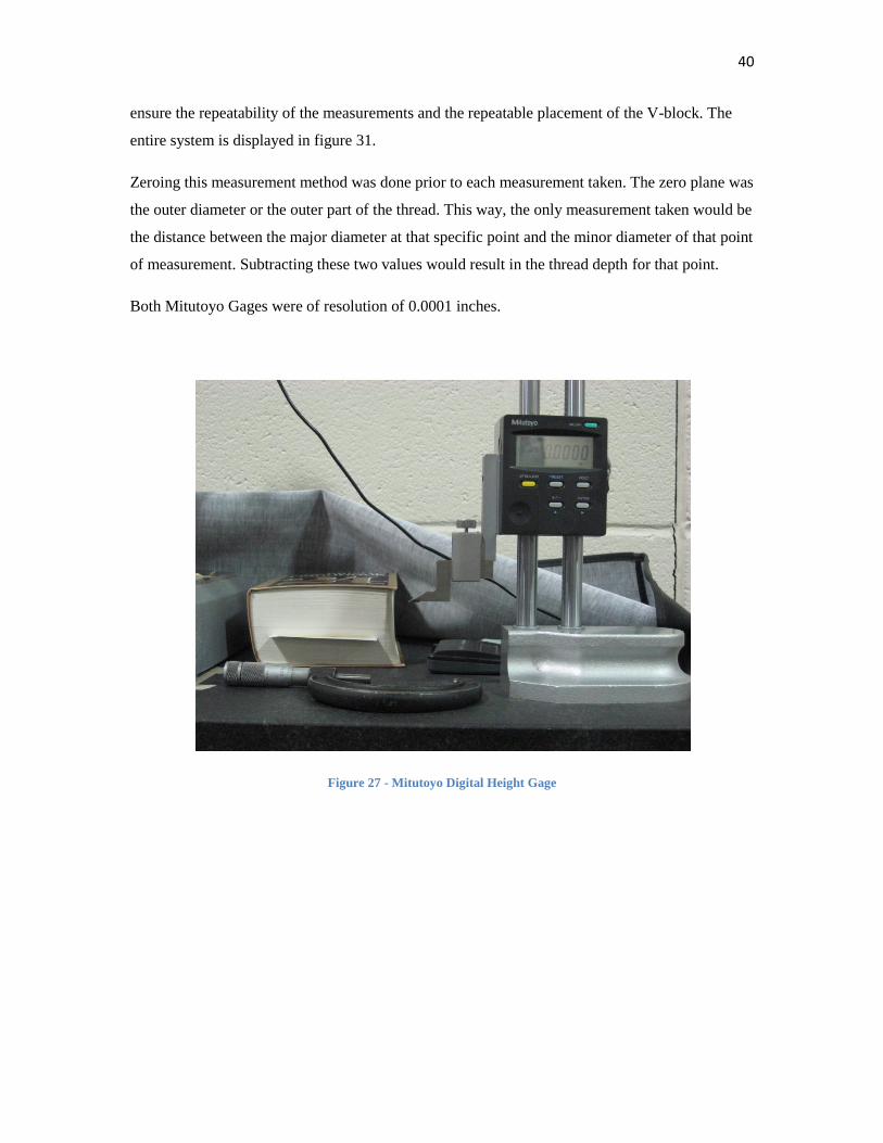
40

ensure the repeatability of the measurements and the repeatable placement of the V-block. The

entire system is displayed in figure 31.

Zeroing this measurement method was done prior to each measurement taken. The zero plane was

the outer diameter or the outer part of the thread. This way, the only measurement taken would be

the distance between the major diameter at that specific point and the minor diameter of that point

of measurement. Subtracting these two values would result in the thread depth for that point.

Both Mitutoyo Gages were of resolution of 0.0001 inches.

Figure 27 - Mitutoyo Digital Height Gage

41

Figure 28 - Close Up of Three Wire Measurement Method

Figure 29 - Three Wire Measurement System

42

Figure 30 - Custom Gage Head for Measuring Thread Depth

Figure 31 - Thread Depth Measurement System

43

This measurement method was the first one developed in order to monitor tool wear with the

target result of identifying which cutting fluid induces the least amount of wear. During the

development of this experiment, the machining parameters were tried out as the data was

gathered.

The initial parameters for both pipe materials were of 15 threading passes per part while using

500 sfm of machining speed. The results of this experiment were gathered in an Excel

spreadsheet displaying each measurement and the side of the part it was taken from. The

following tables (5 and 6) are the results from running the experiment with these machining

parameters. Also displayed are the plots for these results (32, 33, 34, 35, 36 and 37).

All the machining done in this part of the experiment was carried out using one threading insert

per pipe material. The notion was to replace the threading insert once the measurements reached

the specified tolerances supplied in the ACME standard [8]. It was found that after machining 25

L80 parts and 50 P110 parts, the wear induced on the insert was not enough for the results to

show the wear trend.

Table 5 – Data [inch] for L80 Using 15 Passes and 500 sfm

Part

Number

Pipe

Number

Pipe

Type

Cutting

Fluid

type

Outer

Diameter

Start

Outer

Diameter

End

Pitch

Diameter

Measurement

Start

Actual

calculated

Pitch

Diameter -

Start

Pitch Diameter

Measurement

End

Actual

calculated

Pitch

Diameter -

End

Thread

Depth

Start

Thread

Depth

End

1 1 L80 Fuchs 2.3124 2.3125 2.3365 2.2558 2.3350 2.2543 0.0680 0.0680

2 1 L80 Fuchs 2.3125 2.3125 2.3365 2.2558 2.3350 2.2543 0.0680 0.0685

3 1 L80 Fuchs 2.3125 2.3125 2.3365 2.2558 2.3350 2.2543 0.0680 0.0685

4 1 L80 Fuchs 2.3125 2.3125 2.3365 2.2558 2.3355 2.2548 0.0680 0.0685

5 1 L80 Fuchs 2.3125 2.3126 2.3365 2.2558 2.3355 2.2548 0.0680 0.0685

6 1 L80 Fuchs 2.3125 2.3125 2.3365 2.2558 2.3360 2.2553 0.0680 0.0685

7 1 L80 Fuchs 2.3125 2.3124 2.3370 2.2563 2.3360 2.2553 0.0680 0.0685

8 1 L80 Fuchs 2.3124 2.3124 2.3370 2.2563 2.3355 2.2548 0.0680 0.0685

9 1 L80 Fuchs 2.3125 2.3124 2.3370 2.2563 2.3360 2.2553 0.0680 0.0685

10 1 L80 Fuchs 2.3125 2.3124 2.3370 2.2563 2.3360 2.2553 0.0680 0.0685

11 1 L80 Fuchs 2.3125 2.3125 2.3370 2.2563 2.3360 2.2553 0.0680 0.0685

12 1 L80 Fuchs 2.3125 2.3124 2.3370 2.2563 2.3360 2.2553 0.0680 0.0680

13 1 L80 Fuchs 2.3126 2.3125 2.3370 2.2563 2.3360 2.2553 0.0680 0.0685

14 1 L80 Fuchs 2.3126 2.3126 2.3375 2.2568 2.3360 2.2553 0.0680 0.0685

15 2 L80 Fuchs 2.3126 2.3126 2.3370 2.2563 2.3365 2.2558 0.0680 0.0685

16 2 L80 Fuchs 2.3125 2.3125 2.3370 2.2563 2.3365 2.2558 0.0680 0.0685

17 2 L80 Fuchs 2.3125 2.3125 2.3375 2.2568 2.3365 2.2558 0.0680 0.0685

18 2 L80 Fuchs 2.3125 2.3125 2.3375 2.2568 2.3365 2.2558 0.0680 0.0685

19 2 L80 Fuchs 2.3125 2.3126 2.3370 2.2563 2.3365 2.2558 0.0680 0.0680

20 2 L80 Fuchs 2.3125 2.3126 2.3370 2.2563 2.3365 2.2558 0.0680 0.0680

21 2 L80 Fuchs 2.3125 2.3126 2.3370 2.2563 2.3360 2.2553 0.0680 0.0685

22 2 L80 Fuchs 2.3125 2.3126 2.3370 2.2563 2.3360 2.2553 0.0680 0.0685

23 2 L80 Fuchs 2.3125 2.3126 2.3370 2.2563 2.3360 2.2553 0.0680 0.0680

24 2 L80 Fuchs 2.3126 2.3126 2.3375 2.2568 2.3360 2.2553 0.0680 0.0680

25 2 L80 Fuchs 2.3126 2.3126 2.3375 2.2568 2.3365 2.2558 0.0680 0.0685

44

Figure 32 - L80 Outer Diameter Measurements [inch] for 15 Passes and 500 sfm

Figure 33 - L80 Pitch Diameter Measurements [inch] for 15 Passes and 500 sfm

Figure 34 - L80 Thread Depth Measurements [inch] for 15 Passes and 500 sfm

2.3124

2.3124

2.3125

2.3125

2.3126

2.3126

2.3127

0 5 10 15 20 25 30

L80 Outer Diameter Measurements

Outer Diameter Start

Outer Diameter End

2.2540

2.2545

2.2550

2.2555

2.2560

2.2565

2.2570

0 5 10 15 20 25 30

L80 Pitch Diameter Measurements

Actual calculated Pitch Diameter - Start

Actual calculated Pitch Diameter - End

0.0679000

0.0680000

0.0681000

0.0682000

0.0683000

0.0684000

0.0685000

0.0686000

0 5 10 15 20 25 30

L80 Thread Depth Measurements

Thread Depth Start

Thread Depth End

45

Table 6 – Data [inch] for P110 Using 15 Passes and 500 sfm

Part

Number

Pipe

Number

Pipe

Type

Cutting

Fluid

type

Outer

Diameter

Start

Outer

Diameter

End

Pitch

Diameter

Measurement

Start

Actual

calculated

Pitch

Diameter -

Start

Pitch Diameter

Measurement

End

Actual

calculated

Pitch

Diameter -

End

Thread

Depth

Start

Thread

Depth

End

1 2 P110 Fuchs 2.3122 2.3123 2.3380 2.2573 2.3370 2.2563 0.0675 0.0675

2 2 P110 Fuchs 2.3122 2.3122 2.3380 2.2573 2.3360 2.2553 0.0675 0.0675

3 2 P110 Fuchs 2.3122 2.3123 2.3380 2.2573 2.3370 2.2563 0.0675 0.0675

4 2 P110 Fuchs 2.3122 2.3123 2.3380 2.2573 2.3365 2.2558 0.0675 0.0675

5 2 P110 Fuchs 2.3122 2.3122 2.3380 2.2573 2.3360 2.2553 0.0675 0.0675

6 2 P110 Fuchs 2.3122 2.3122 2.3380 2.2573 2.3365 2.2558 0.0675 0.0675

7 2 P110 Fuchs 2.3122 2.3122 2.3380 2.2573 2.3365 2.2558 0.0675 0.0675

8 2 P110 Fuchs 2.3123 2.3122 2.3380 2.2573 2.3370 2.2563 0.0675 0.0675

9 2 P110 Fuchs 2.3123 2.3123 2.3380 2.2573 2.3370 2.2563 0.0675 0.0675

10 2 P110 Fuchs 2.3123 2.3124 2.3380 2.2573 2.3365 2.2558 0.0675 0.0675

11 2 P110 Fuchs 2.3123 2.3124 2.3380 2.2573 2.3365 2.2558 0.0675 0.0675

12 2 P110 Fuchs 2.3123 2.3124 2.3380 2.2573 2.3360 2.2553 0.0675 0.0675

13 2 P110 Fuchs 2.3123 2.3125 2.3380 2.2573 2.3365 2.2558 0.0675 0.0675

14 3 P110 Fuchs 2.3125 2.3125 2.3380 2.2573 2.3370 2.2563 0.0670 0.0680

15 3 P110 Fuchs 2.3126 2.3125 2.3380 2.2573 2.3370 2.2563 0.0675 0.0680

16 3 P110 Fuchs 2.3126 2.3125 2.3380 2.2573 2.3375 2.2568 0.0675 0.0680

17 3 P110 Fuchs 2.3125 2.3125 2.3380 2.2573 2.3375 2.2568 0.0675 0.0680

18 3 P110 Fuchs 2.3125 2.3125 2.3375 2.2568 2.3370 2.2563 0.0675 0.0680

19 3 P110 Fuchs 2.3125 2.3124 2.3375 2.2568 2.3365 2.2558 0.0675 0.0680

20 3 P110 Fuchs 2.3125 2.3125 2.3370 2.2563 2.3360 2.2553 0.0675 0.0680

21 3 P110 Fuchs 2.3125 2.3125 2.3370 2.2563 2.3360 2.2553 0.0680 0.0680

22 3 P110 Fuchs 2.3125 2.3123 2.3370 2.2563 2.3360 2.2553 0.0680 0.0685

23 3 P110 Fuchs 2.3125 2.3124 2.3370 2.2563 2.3360 2.2553 0.0680 0.0685

24 3 P110 Fuchs 2.3125 2.3124 2.3370 2.2563 2.3360 2.2553 0.0680 0.0685

25 3 P110 Fuchs 2.3125 2.3126 2.3375 2.2568 2.3365 2.2558 0.0680 0.0685

26 3 P110 Fuchs 2.3125 2.3125 2.3370 2.2563 2.3365 2.2558 0.0680 0.0685

27 3 P110 Fuchs 2.3124 2.3124 2.3370 2.2563 2.3360 2.2553 0.0680 0.0685

28 3 P110 Fuchs 2.3125 2.3125 2.3370 2.2563 2.3355 2.2548 0.0680 0.0685

29 4 P110 Fuchs 2.3122 2.3125 2.3370 2.2563 2.3355 2.2548 0.0680 0.0680

30 4 P110 Fuchs 2.3122 2.3125 2.3365 2.2558 2.3360 2.2553 0.0680 0.0685

31 4 P110 Fuchs 2.3122 2.3123 2.3370 2.2563 2.3360 2.2553 0.0680 0.0680

32 4 P110 Fuchs 2.3122 2.3122 2.3370 2.2563 2.3355 2.2548 0.0680 0.0680

33 4 P110 Fuchs 2.3123 2.3123 2.3370 2.2563 2.3355 2.2548 0.0680 0.0680

34 4 P110 Fuchs 2.3124 2.3122 2.3370 2.2563 2.3355 2.2548 0.0675 0.0680

35 4 P110 Fuchs 2.3124 2.3123 2.3370 2.2563 2.3360 2.2553 0.0680 0.0680

36 4 P110 Fuchs 2.3123 2.3123 2.3375 2.2568 2.3360 2.2553 0.0680 0.0680

37 4 P110 Fuchs 2.3123 2.3124 2.3375 2.2568 2.3360 2.2553 0.0680 0.0680

38 4 P110 Fuchs 2.3123 2.3122 2.3375 2.2568 2.3365 2.2558 0.0680 0.0685

39 4 P110 Fuchs 2.3123 2.3123 2.3380 2.2573 2.3365 2.2558 0.0675 0.0680

40 4 P110 Fuchs 2.3123 2.3123 2.3380 2.2573 2.3365 2.2558 0.0680 0.0680

41 4 P110 Fuchs 2.3124 2.3123 2.3380 2.2573 2.3365 2.2558 0.0680 0.0680

42 4 P110 Fuchs 2.3124 2.3123 2.3380 2.2573 2.3370 2.2563 0.0675 0.0680

43 5 P110 Fuchs 2.3123 2.3123 2.3380 2.2573 2.3365 2.2558 0.0675 0.0680

44 5 P110 Fuchs 2.3123 2.3123 2.3380 2.2573 2.3365 2.2558 0.0675 0.0680

45 5 P110 Fuchs 2.3123 2.3124 2.3375 2.2568 2.3365 2.2558 0.0675 0.0680

46 5 P110 Fuchs 2.3123 2.3125 2.3380 2.2573 2.3365 2.2558 0.0675 0.0680

47 5 P110 Fuchs 2.3124 2.3125 2.3380 2.2573 2.3370 2.2563 0.0680 0.0685

48 5 P110 Fuchs 2.3124 2.3124 2.3380 2.2573 2.3365 2.2558 0.0680 0.0685

49 5 P110 Fuchs 2.3125 2.3124 2.3380 2.2573 2.3365 2.2558 0.0680 0.0685

50 5 P110 Fuchs 2.3125 2.3124 2.3380 2.2573 2.3370 2.2563 0.0680 0.0685

46

Figure 35 - P110 Outer Diameter Measurements [inch] for 15 Passes and 500 sfm

Figure 36 - P110 Pitch Diameter Measurements [inch] for 15 Passes and 500 sfm

Figure 37 - P110 Thread Depth Measurements [inch] for 15 Passes and 500 sfm

2.3122

2.3122

2.3123

2.3123

2.3124

2.3124

2.3125

2.3125

2.3126

2.3126

2.3127

0 10 20 30 40 50 60

P110 Outer Diameter Measurements


Outer Diameter End

2.2545

2.2550

2.2555

2.2560

2.2565

2.2570

2.2575

0 10 20 30 40 50 60

P110 Pitch Diameter Measurements

Actual calculated Pitch Diameter -Start

Actual calculated Pitch Diameter -End

0.0668

0.0670

0.0672

0.0674

0.0676

0.0678

0.0680

0.0682

0.0684

0.0686

0 10 20 30 40 50 60

P110 Thread Depth Measurements

Thread Depth Start

Thread Depth End

47

It was decided to try and induce more wear on the inserts by increasing the SFM in the machining

cycle. When running trial and error programs, it was found that with 650 SFM it was possible to

machine 12 parts, and perhaps induce enough wear on the inserts. The following tables (7 and 8)

and plots (figures 38, 29, 40, 41, 42 and 43) are the results for running both L80 and P110 on the

new program.

For L80 the results are as follows:

Table 7 – Data [inch] for L80 Using 15 Passes and 650 sfm

Figure 38 - L80 Outer Diameter Measurements [inch] for 15 Passes and 650 sfm

Part

Number

Pipe

Number

Pipe

Type

Cutting

Fluid

type

Outer

Diameter

Start

Outer

Diameter

End

Pitch

Diameter

Measurement

Start

Actual

calculated

Pitch

Diameter -

Start

Pitch Diameter

Measurement

End

Actual

calculated

Pitch

Diameter -

End

Thread

Depth

Start

Thread

Depth

End

1X 3 L80 Fuchs 2.3121 2.3123 2.3400 2.2593 2.3395 2.2588 0.0670 0.0675

2X 3 L80 Fuchs 2.3122 2.3124 2.3400 2.2593 2.3400 2.2593 0.0670 0.0675

3X 3 L80 Fuchs 2.3122 2.3123 2.3400 2.2593 2.3400 2.2593 0.0670 0.0675

4X 3 L80 Fuchs 2.3123 2.3123 2.3405 2.2598 2.3400 2.2593 0.0670 0.0675

5X 3 L80 Fuchs 2.3123 2.3123 2.3410 2.2603 2.3400 2.2593 0.0675 0.0675

6X 3 L80 Fuchs 2.3123 2.3123 2.3405 2.2598 2.3395 2.2588 0.0675 0.0675

7X 3 L80 Fuchs 2.3123 2.3123 2.3405 2.2598 2.3400 2.2593 0.0675 0.0675

8X 3 L80 Fuchs 2.3124 2.3123 2.3410 2.2603 2.3400 2.2593 0.0675 0.0675

9X 3 L80 Fuchs 2.3124 2.3123 2.3410 2.2603 2.3395 2.2588 0.0675 0.0675

10X 3 L80 Fuchs 2.3124 2.3122 2.3410 2.2603 2.3395 2.2588 0.0675 0.0675

11X 3 L80 Fuchs 2.3124 2.3122 2.3410 2.2603 2.3395 2.2588 0.0675 0.0675

12X 3 L80 Fuchs 2.3124 2.3122 2.3410 2.2603 2.3395 2.2588 0.0675 0.0675

13X 3 L80 Fuchs 2.3124 2.3123 2.3410 2.2603 2.3395 2.2588 0.0675 0.0675

14X 3 L80 Fuchs 2.3125 2.3123 2.3410 2.2603 2.3395 2.2588 0.0675 0.0675

15X 4 L80 Fuchs 2.3125 2.3123 2.3410 2.2603 2.3400 2.2593 0.0675 0.0675

16X 4 L80 Fuchs 2.3125 2.3123 2.3415 2.2608 2.3400 2.2593 0.0675 0.0675

17X 4 L80 Fuchs 2.3125 2.3123 2.3415 2.2608 2.3400 2.2593 0.0675 0.0675

18X 4 L80 Fuchs 2.3125 2.3123 2.3415 2.2608 2.3405 2.2598 0.0675 0.0675

19X 4 L80 Fuchs 2.3125 2.3124 2.3425 2.2618 2.3400 2.2593 0.0675 0.0675

2.3121

2.3121

2.3122

2.3122

2.3123

2.3123

2.3124

2.3124

2.3125

2.3125

2.3126

0 5 10 15 20

L80 Outer Diameter Measurements


Outer Diameter End

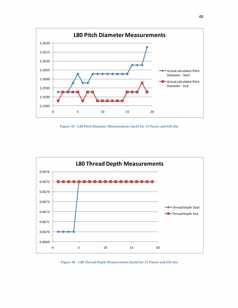
48

Figure 39 - L80 Pitch Diameter Measurements [inch] for 15 Passes and 650 sfm

Figure 40 - L80 Thread Depth Measurements [inch] for 15 Passes and 650 sfm

2.2585

2.2590

2.2595

2.2600

2.2605

2.2610

2.2615

2.2620

0 5 10 15 20

L80 Pitch Diameter Measurements



0.0669

0.0670

0.0671

0.0672

0.0673

0.0674

0.0675

0.0676

0 5 10 15 20

L80 Thread Depth Measurements

Thread Depth Start

Thread Depth End

49

For P110 the results are as follows:

Table 8 – Data [inch] for P110 Using 15 Passes and 650 sfm

The reduction in the Outer Diameter is a result in an offset change while running the machining

program. This was done while monitoring the change in the Outer Diameter between each of the

parts machined.

Figure 41 - P110 Outer Diameter Measurements [inch] for 15 Passes and 650 sfm

Part

Number

Pipe

Number

Pipe

Type

Cutting

Fluid

type

Outer

Diameter

Start

Outer

Diameter

End

Pitch

Diameter

Measurement

Start

Actual

calculated

Pitch

Diameter -

Start

Pitch Diameter

Measurement

End

Actual

calculated

Pitch

Diameter -

End

Thread

Depth

Start

Thread

Depth

End

1P 6 P110 Fuchs 2.3125 2.3125 2.3395 2.2588 2.3380 2.2573 0.0675 0.0670

2P 6 P110 Fuchs 2.3142 2.3131 2.3400 2.2593 2.3390 2.2583 0.0675 0.0675

3P 6 P110 Fuchs 2.3133 2.3118 2.3400 2.2593 2.3380 2.2573 0.0675 0.0670

4P 6 P110 Fuchs 2.3135 2.3122 2.3400 2.2593 2.3380 2.2573 0.0675 0.0670

5P 6 P110 Fuchs 2.3134 2.3126 2.3400 2.2593 2.3380 2.2573 0.0675 0.0670

6P 6 P110 Fuchs 2.3136 2.3122 2.3400 2.2593 2.3385 2.2578 0.0675 0.0665

7P 6 P110 Fuchs 2.3136 2.3125 2.3405 2.2598 2.3380 2.2573 0.0675 0.0665

8P 6 P110 Fuchs 2.3141 2.3131 2.3400 2.2593 2.3390 2.2583 0.0680 0.0665

9P 6 P110 Fuchs 2.3145 2.3134 2.3405 2.2598 2.3385 2.2578 0.0680 0.0670

10P 6 P110 Fuchs 2.3146 2.3134 2.3400 2.2593 2.3380 2.2573 0.0680 0.0670

11P 6 P110 Fuchs 2.3145 2.3137 2.3400 2.2593 2.3380 2.2573 0.0680 0.0675

12P 6 P110 Fuchs 2.3146 2.3134 2.3405 2.2598 2.3385 2.2578 0.0675 0.0670

13P 7 P110 Fuchs 2.3147 2.3146 2.3400 2.2593 2.3380 2.2573 0.0680 0.0670

14P 7 P110 Fuchs 2.3155 2.3148 2.3400 2.2593 2.3400 2.2593 0.0675 0.0675

15P 7 P110 Fuchs 2.3157 2.3147 2.3410 2.2603 2.3400 2.2593 0.0680 0.0675

16P 7 P110 Fuchs 2.3157 2.3149 2.3410 2.2603 2.3400 2.2593 0.0685 0.0675

17P 7 P110 Fuchs 2.3157 2.3152 2.3415 2.2608 2.3400 2.2593 0.0685 0.0670

18P 7 P110 Fuchs 2.3161 2.3152 2.3415 2.2608 2.3390 2.2583 0.0595 0.0595

19P 7 P110 Fuchs 2.3160 2.3153 2.3415 2.2608 2.3400 2.2593 0.0550 0.0550

2.3115

2.3120

2.3125

2.3130

2.3135

2.3140

2.3145

2.3150

2.3155

2.3160

2.3165

0 5 10 15 20

P110 Outer Diameter Measuremets


Outer Diameter End

50

Figure 42 - P110 Pitch Diameter Measurements [inch] for 15 Passes and 650 sfm

Figure 43 - P110 Thread Depth Measurements [inch] for 15 Passes and 650 sfm

2.2570

2.2575

2.2580

2.2585

2.2590

2.2595

2.2600

2.2605

2.2610

0 5 10 15 20

P110 Pitch Diameter Measurements



0.0000

0.0100

0.0200

0.0300

0.0400

0.0500

0.0600

0.0700

0.0800

0 5 10 15 20

P110 Thread Depth Measurements

Thread Depth Start

Thread Depth End

51

When studying the results from the different program speeds, for both pipe materials, it was

noticed that there are continuous inconsistencies in the growth and changes in the parts

dimensions. Unlike hypothesized, the dimensions were changing to both larger and smaller values

with no apparent consistency.

Looking deeper into result trends, it was concluded that there are two problems which might

cause this measurement method to fail:

1. Resolution of measurement equipment. The changes in the threading insert as well as the

dimensional changes in the work materials may be occurring at a size scale that is lower

than can be measured with contact measurement.

2. A different physical phenomenon was affecting the experiment and thus the results.

The second problem resulted in the discovery of the egg shaped pipe described in section 4.1

Threading Process and lead to the development of the Image Processing Tool Wear measurement

method.

4.4 Experiment Design

In the general experiment design, it was decided that each cutting fluid would be independently

tested with each pipe grade. An experiment involved using an insert to machine a fixed number

of sample threaded parts. Afterwards, the tool wear variables previously discussed would be

measured. Based on the tool wear data derived from preliminary experiments, it was determined

that the machining of eighteen sample parts was sufficient to generate significant tool wear when

machining API L80 pipe. Twelve sample parts were sufficient when machining the API P110

pipe. Each experiment involving a cutting fluid-pipe grade combination was to be replicated ten

times.

While running pilot cycles on both pipe grades, it was found that many of the raw pipes were egg

shaped. This shape remained even after the turning passes were conducted on the raw pipe.

Increasing the depth of the turning passes would reduce the pipe wall thickness to a point that the

part becomes too flexible, a fact that would affect the threading cycles and the stresses induced on

the threading inserts. There was a need to randomize the process of using the raw pipe in order to

remove the pipe shape issue from the experiment entirely.

52

It was not practical to completely randomize this experiment. This was due to the limited

quantities of cutting fluid available and the fact that the turning center reservoir had to be filled to

fifty gallons. Furthermore it was very time consuming to flush out the reservoir and prepare a

new batch of mixture. As a consequence, the turning center was filled with a specific cutting

fluid mixture only one time. During that period, ten replicate experiments involving that specific

cutting fluid and API L80 pipe were run consecutively. This was followed by ten consecutive

replicates involving the API P110 pipe.

In order to cope with the egg shape pipe issue, a randomization process was planned into the

experiment. Five different cutting fluids were to be compared. In order to make sure each cutting

fluid was used to machine the same percentage of egg shaped pipe, each pipe was used for

machining parts with all five cutting fluids. For example, from one pipe (pipe A), two parts were

machined using cutting fluid #1. This pipe would then be placed at a ―used-pipe‖ pile. When

switching to the next liquid (#2), pipe A would be retrieved and another two parts were machined

using liquid #2, and so on for the five cutting fluids.

Aside from the randomization process described above, all other external factors were adequately

controlled so that the variation in the wear results is due solely to the effects of the cutting fluids.

For cutting fluid QC2776, there were 5 threading edges used for material API P110 instead of the

usual 10 edges. This is due to the fact that this fluid was not performing as well as other liquids

tested when machining L80. A decision was made to stop the use of this cutting fluid after half

the repetitions as to not waste material and reduce the overall cost of the experiment when it was

already known that QC2776 was inferior.

53

Chapter 5

RESULTS

Five cutting fluids (EcoCool, MC3680, QC2776, QC7035 and QC7102) were tested on two pipe

grades (API L80, API P110). A total of one hundred sets of threading edges from fifty threading

inserts were used. Each edge was used to machine eighteen parts for pipe grade API L80 or

twelve parts for pipe grade API P110.

Five of the repetitions resulted in tool fracture. In four of the cases, no gradual wear data could be

collected. In one of the cases, the edge chipped while machining the last part. It was chipped in

such a way that some of the required data was still retrievable and used in the overall analysis.

A summary of these tool fractures is presented in Table 9. Columns two and four identify the

number of fractured edges that resulted from each combination of cutting fluid and pipe grade.

Columns three and five indicate the number of parts that were completed prior to the fracture.

As can be seen, the use of QC2776 in combination with the L80 pipe grade resulted in tool

fracture in three of the ten repetitions. The other two cases involved EcoCool in combination with

the L80 pipe grade and the MC3680 and the P110 pipe grade.

Table 9 - Summary of Broken Threading Edges

QC7102 and QC7035 were the only fluids used that did not result in tool fracture for any of the

repetitions.

Five of the one hundred repetitions were not completed due to a decision to stop the experiments

involving QC2776 and API P110 pipe. This decision was made because the cutting fluid

performed poorly with the API L80 pipe, and was performing even worse with the P110 pipe. It

made little sense to waste the material and time to further characterize it.

Cutting Fluid L80

Number of parts

completed with

broken edge

P110

Number of parts

completed with

broken edge

Fuch EcoCool 1 7 0

QC7102 0 0

QC7035 0 0

QC2776 3 9, 18, 16 0

Microcut 3680 0 1 12

54

With regard to the replicates for which gradual wear measurements were taken, the data was

collected and stored in a large spreadsheet. These results were analyzed using the statistical

analysis software JMP. All of the results are displayed in Appendix B. The results are explained

in the following sections.

5.1 Tool Wear Data Presentation and Interpretation of Statistical Analysis Results

The measurements and analysis for all wear variables are displayed in Appendix B for each

combination of cutting fluid and pipe grade. The data is organized by wear variable. The

complete results for all cutting fluids for each pipe grade are organized under each wear variable

heading. The results include a wear measurement data summary table, a means comparison plot,

and a comparison of means statistical analysis table.

Table 10 provides an example of a data summary table. The five columns display the wear

measurements for the five respective fluids. A red cell indicates a threading tool edge that was

broken while machining and therefore no data could be collected from that edge. An empty cell

indicates an edge that was not used as described earlier in this report (e.g. QC 2776). A cell with a

value of ‗0‘ represents a measurement with a value of ‗0‘ – no wear at all.

Table 10 - Summary of Experimental Measurements Table for Rake Face –Tool Wear-Wear Area (mm^2)

Fuchs QC 7102 QC 2776 QC 7035 MC 3680

0.1300 0.1000 0.1100 0.1300 0.1300

0.1000 0.1000 0.1300 0.1200

0.1100 0.0800 0.1200 0.1300 0.1300

0.1002 0.1200 0.1100 0.1300

0.1300 0.0900 0.1300 0.1200 0.1400

0.1400 0.0800 0.1300 0.1300 0.1200

0.1200 0.0800 0.1200 0.1100 0.1600

0.1000 0.0700 0.1100 0.1100 0.1300

0.1100 0.1000 0.1000 0.1200

0.1000 0.1100 0.1200 0.1200

55

This data was fed into the JMP statistical analysis software to generate a comparison of means

plot such as the one illustrated in Figure 44. The plot displays the measurement data for each

fluid. The grey line crossing the entire plot is the grand mean for all samples. The blue line

connects the samples mean for each cutting fluid.

For each combination of wear variable and pipe grade, a statistical comparison of means test was

executed to determine whether differences in the sample means were due to true differences in

the performances of the cutting fluids rather than just pure chance. Ordinarily it is desired to run

a parametric test such as the Student T comparison of means test. A parametric test provides the

greatest amount of detection resolution. However, to use such a test reliably requires a priori

knowledge of the type of probability distribution that describes each sample. For example, to use

the Student T test, it must be assumed that each sample is normally distributed. Furthermore, it

must be assumed that the variances of the distributions are equal or not.

Figure 44 - Means Comparison Plot

In order to reliably assess the type of a probability distribution requires a sample size of at least

forty. Unfortunately for this investigation, only ten were available at most for each sample.

Because of this fact, a nonparametric comparison of means test was employed. The test that was

used was the Wilcoxon Rank Sum test. The assumption behind this test is that the two samples

being compared are derived from distributions that are equal in form and variance. Based on

observations of the data distributions in the comparison of means plots, it was felt that this was a

reasonable assumption to make.

Instead of using the original values of tool wear, the Wilcoxon Test uses a new variable or

ranking system, the ―rank score‖. The actual means are assigned a score from one to the number

56

of the observations, starting from the lowest mean. The Score Sum and Score Mean are the sum

and average of these ranked scores. The score means are standardized. In this method the ranks

are used to analyze the data instead of the actual data.

The level of confidence (1 – α) of this test was set to ninety-five percent (e.g. α = .05). This

implies that for differences in means that exceed the critical value, there is a ninety-five percent

probability that this resulted from differences in cutting fluid performance rather than pure

chance.

An example of the results of this test is presented in Table 11. The results parameters/variables

are as follows [7]:

q* - Gives the quintile value used in the confidence intervals.

Alpha – Gives the alpha level used in the confidence intervals.

Level – Gives the pair used in the current comparison.

Score Mean Difference – Gives the difference of the score means.

STD Err Diff – Gives the standard error of the difference between the score means.

Z – Gives the standardized test statistic, which has an asymptotic standard normal

deviation under the null hypothesis.

P-Value – Gives the asymptotic two-sided p-Value for Z.

Hodges-Lehmann – Gives the Hodges-Lehmann estimator of location shift. It is the

median of all paired differences between observations in the two sided samples.

Table 11 - Wilcoxon Rank Test Results

The table lists ten pair-wise comparisons. Comparisons for which the p-Value is less than .05 are

identified as having a statistical difference. These are also identified by a * next to the value.

57

Some of the Wilcoxon data tables (Table 32 for example) have no values in the Z and p-Value

columns. This occurs when the values of the compared liquids are identical and the standard

deviation is zero, hence the Z and p-Values are missing.

5.2 Analysis Summary and Conclusions of Results

Table 12 provides a summary of the comparison of means tests for all experiments involving API

L80 pipe. Red cells mark the lowest sample mean for that wear variable. A yellow cell indicates a

statistically significant difference between the fluid with the lowest mean and the mean associated

with Fuchs EcoCool. A green cell indicates a statistically significant difference between the fluid

with the lowest mean and each of the means associated with the other four fluids. For example,

for the wear variable Rake Face-Tool Wear-Wear Area (mm^2), QC7102 has the lowest sample

mean. Furthermore, its mean value is statistically different than the means associated with the

other four fluids.

Observation of Table 12 reveals that QC7102 has the lowest sample mean for eight of the eleven

wear variables. Furthermore, in four of these cases, the mean is statistically lower than the means

of the other four fluids. When directly compared to EcoCool, this number jumps to six.

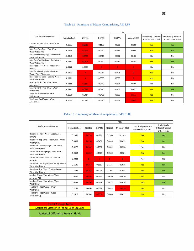
58

Lowest Average Mean

Statistical Difference From Fuchs EcoCool

Statistical Difference From all Fluids

Table 12 - Summary of Means Comparisons, API L80

Table 13 - Summary of Means Comparisons, API P110

Fuchs EcoCool QC7102 QC7035 QC2776 Microcut 3860Statistically Different

form Fuchs EcoCool

Statistically Different

from all Other Fluids

Rake Face - Tool Wear - Wear Area

(mm^2)0.1156 0.0910 0.1190 0.1200 0.1300 Yes Yes

Rake Face Top Edge - Tool Wear -

Wear Width(mm)0.0373 0.0292 0.0420 0.0385 0.0440 Yes Yes

Rake Face Leading Edge - Tool Wear -

Wear Width(mm)0.0319 0.0299 0.0410 0.0362 0.0406 No No

Rake Face Trailing Edge - Tool Wear -


Rake Face - Tool Wear - Crater area

(mm^2)0.0053 0.0030 0 0 0 No No

Rake Face Leading Edge - Coating

Wear - Wear Width(mm)0.1911 0 0.0087 0.0428 0 Yes No

Rake Face Top Edge - Coating Wear -

Wear Width(mm)0.1881 0 0.0090 0.0390 0 Yes No

Leading Flank - Tool Wear - Wear

Area(mm^2)0.0444 0.0410 0.0440 0.0514 0.0480 No No


Width(mm)0.0381 0.0313 0.0416 0.0457 0.0423 Yes Yes

Top Flank - Tool Wear - Wear

Width(mm)0.1118 0.0417 0.0433 0.0500 0.0373 Yes No


Area(mm^2)0.1100 0.0570 0.0480 0.0543 0.0460 Yes No

Performance Measure

L80

Fuchs EcoCool QC7102 QC7035 QC2776 Microcut 3860Statistically Different

form Fuchs EcoCool

Statistically

Different from all

Other Fluids


(mm^2)0.1050 0.0726 0.1220 0.1160 0.1189 Yes Yes

Rake Face Top Edge - Tool Wear - Wear

Width(mm)0.0403 0.0296 0.0430 0.0393 0.0429 Yes Yes

Rake Face Leading Edge - Tool Wear -

Wear Width(mm)0.0272 0.0246 0.0390 0.0332 0.0328 No No

Rake Face Trailing Edge - Tool Wear -


Rake Face - Tool Wear - Crater area

(mm^2)0.0044 0 0 0 0 No No

Rake Face Leading Edge - Coating Wear -


Rake Face Top Edge - Coating Wear -



Area(mm^2)0.0460 0.0360 0.0440 0.0440 0.0470 Yes No


Width(mm)0.0396 0.0290 0.0406 0.0373 0.0416 Yes Yes


Width(mm)0.1266 0.0650 0.0536 0.0533 0.0529 Yes No


Area(mm^2)0.1310 0.0740 0.0550 0.0580 0.0611 Yes No

Performance Measure

P110

59

Table 13 provides a summary of the comparison of means tests for all experiments involving API

P110 pipe. These results indicate that QC7102 has the lowest sample mean for nine of the eleven

wear variables. In six of these cases, the mean is statistically lower than the means of the other

four fluids. When directly compared to EcoCool, this number jumps to seven.

Based on the results presented in Tables 12 and 13, it is clear that QC7102 was by far the best

cutting fluid tested for both pipe grades. A direct comparison between QC7102 and EcoCool is

presented in Table 14.

When threading API L80 pipe, the use of QC7102 in lieu of EcoCool reduced tool wear by an

amount ranging from 6.22 percent to 100 percent with regard to the eleven wear variables. The

average reduction in tool wear for all eleven wear variables was 48.3 percent. For processes

involving API P110 pipe, the reduction in tool wear ranged from 9.54 percent to 100 percent,

with an average of 45.8 percent.

Based on these results, there is strong evidence that TMK-IPSCO could reap significant benefits

by switching from EcoCool to QC7102. Of course, if they do, this would imply that QC7102 will

be used for all other processes carried out in their pipe machining cycle. It is doubtful that the use

of QC7102 will lead to poorer tool wear in these cases. Nevertheless, TMK-IPSCO should run a

trial study in which QC7102 is used.

Table 14 - Comparison between QC7102 and EcoCool

Lower Mean Statistically Significant Wear reduction Percentage % Lower Mean Statistically Significant Wear reduction Percentage %


(mm^2)QC7102 Yes 21.24 QC7102 Yes 30.82

Rake Face Top Edge - Tool Wear -

Wear Width(mm)QC7102 Yes 21.71 QC7102 Yes 26.65

Rake Face Leading Edge - Tool

Wear - Wear Width(mm)QC7102 No 6.22 QC7102 No 9.54

Rake Face Trailing Edge - Tool

Wear - Wear Width(mm)QC7102 Yes 45.76 QC7102 Yes 85.34

Rake Face - Tool Wear - Crater

area (mm^2)QC7102 No 43.28 QC7102 No 100

Rake Face Leading Edge - Coating

Wear - Wear Width(mm)QC7102 Yes 100 QC7102 Yes 68.01

Rake Face Top Edge - Coating

Wear - Wear Width(mm)QC7102 Yes 100 QC7102 Yes 42.57


Area(mm^2)QC7102 No 7.75 QC7102 Yes 21.74


Width(mm)QC7102 Yes 17.90 QC7102 Yes 26.88


Width(mm)QC7102 Yes 62.75 QC7102 Yes 48.68


Area(mm^2)QC7102 Yes 48.18 QC7102 Yes 43.51

L80 P110Performance Measure

60

5.3 Discussion of Measurement Methods

This thesis presents three measurement methods used to quantify the amount of tool wear induced

on a threading insert while machining ACME 8P threads using different cutting fluids. These

three methods were developed in an attempt to distinguish and measure the different effects of the

cutting fluids on the tool wear rate in order to increase the efficiency of the threading process.

The first method developed, Part Dimension Changes (section 4.3.3), quantifies tool wear rate

based on the geometric dimensions of the part machined. This method incorporates measuring

predefined dimensions related to the part which are defined by the ACME 8P standard. The data

collected has allowed the identification of a systematic error in the method design – the perfect

roundness of the raw pipe material.

The discovery of the egg shaped pipe resulted in the discontinuation of using the Part Dimension

Changes method due to discrepancies in the data collected which had direct effect on the ultimate

result of the experiment, identifying a way to distinguish between cutting fluid effects on tool

wear rate.

The second measurement method developed, Tool Weight Loss (section 4.3.2), is based on the

weight loss of the threading insert used in the machining process. As the threading insert wears, it

losses weight as a result of material being worn off due to the stresses applied during the

machining process. This method provided a smaller amount of data compared to the other

methods used in this investigation which required a deeper analysis to reach some of the

conclusions. With the experiment designed in this project it was impossible to identify the

superiority of one cutting fluid over the others. This is due to the small number of repetitions

performed, the resolution of the scale used and the effects of other phenomena which may affect

the results and need to be investigated separately (built up edge for example).

Overall, it was concluded not to use this method to determine the superiority of a cutting fluid in

reducing insert wear rate.

The third and preferred measurement method developed for measuring the effectiveness of

cutting fluid reduction of tool wear was the Image Processing Tool Wear Measurement System

(section 4.3.1). This method used a digital image processing system combined with a microscope

in order to accurately measure the wear on the threading inserts. Wear variables wear developed

61

in order to assess the different wear induced on the insert at different areas of the insert. This

wear affects the final geometry of the threaded part and thus was monitored.

The images taken using the system were analyzed using specialized software and data was

generated regarding the quantification of the wear for each variable. This data was statistically

analyzed and one cutting fluid was found to be superior to other cutting fluids used in this

experiment. This fluid was the Quaker Fluid QC7102.

Using this measurement method it was found that accurate and repeatable measurements could be

taken and thus provide a basis for a thorough analysis of the data.

5.4 General Observations

In addition to the results described thus far, a few additional observations are worth noting.

1. The pipe machined in this experiment creates chips that are very difficult to manage for

the machine operator. The chips do no break and occasionally wrap around the part,

chuck, tool holders etc. as shown in Figure 45. The chips are very long and flexible and

bunch up into large metal wire balls, which get stuck in the machine when an attempt is

made to auger them out. This requires the operator to stop the machining process in order

to remove these chips from the machine manually. This operation increased the overall

experiment time and was a safety issue for the operator.

Figure 45 - Example of Stringy Chips Wrapping Around Different Parts of the Machine

62

2. While using QC7035, it was noticed that it evaporated significantly faster compared to the

other cutting fluids. This issue caused the operator to stop machining in order to re-fill the

machine with more mixture. This operation was needed only when using QC7035.

3. Microcut 3680 has a significantly stronger, unpleasant smell when compared to the other

cutting fluids.

63

Chapter 6

FUTURE RESEARCH

Based on the evidence and observations gained in this investigation, the following opportunities

arise for future research projects:

1. Conduct a trial study in which QC7102 cutting fluid is used in the pipe machining

process. During this study, all the relevant process performance metrics should be

monitored and tracked. These metrics can then be compared to those derived with the

Fuchs EcoCool. Based on the evidence gained in this investigation, the use of QC7102

fluid may lead to significant improvements in machining lead time, quality, and cost.

2. The current design of the High Tech Tool threading insert used by TMK-IPSCO does not

incorporate a chip breaker. This is similar to the ACME 8P threading insert used in this

investigation. Designing a chip breaker into the threading inserts should be investigated.

If proven effective, the use of a chip breaker could significantly reduce the machine

downtime necessary to clear out chips from the machine. It would also reduce the safety

hazard to the operators.

3. It is well known that gradual tool wear is highly sensitive to cutting speed [6]. The

greater the cutting speed, the greater the wear rate, and the greater the downtime

necessary for tool replacement. Alternatively, machining cycle time is inversely

proportional to cutting speed. Consequently, cutting speed has a mixed but significant

effect on the total lead time necessary to thread a pipe.

The same holds true with regard to the number of in-feeds used to generate the thread as

well as the in-feed method (e.g. constant d.o.c. versus constant chip load). Both variables

are known to significantly impact thread quality and the rate of threading insert wear. All

of these facts were borne out during the development of the threading process used in this

investigation. Consequently, it is highly recommended to attempt to fine tune these

variables for the specific threading processes if it was not done already. This is true for

the currently used cutting fluid as well as for the QC7102 cutting fluid.

4. The Part Dimension Measurement method described in this thesis (section 4.3.4) could

result in an efficient and accurate measurement method if performed on round pipe.

64

APPENDIX A – TITRATION METHODS FOR EACH CUTTING FLUID

Figure 46 - Titration Method for Fuchs EcoCool

65

Figure 47 - Titration Method for QC7035

66


67


68

Figure 50 - Titration Method for Microcut 3680

69

APPENDIX B – RESULT TABLES AND PLOTS FOR EACH WEAR VARIABLE

The following data is the raw data and means comparisons plots for all wear variables and pipe

materials.

Rake Face – Tool Wear - Wear Area (mm^2)

L80 –

Table 15 – Raw Data for Rake Face – Tool Wear - Wear Area (mm^2), API L80

Figure 51 - Means Comparison Rake Face – Tool Wear - Wear Area (mm^2), API L80

Fuchs QC 7102 QC 2776 QC 7035 MC 3680

0.1300 0.1000 0.1100 0.1300 0.1300

0.1000 0.1000 0.1300 0.1200

0.1100 0.0800 0.1200 0.1300 0.1300

0.1002 0.1200 0.1100 0.1300

0.1300 0.0900 0.1300 0.1200 0.1400

0.1400 0.0800 0.1300 0.1300 0.1200

0.1200 0.0800 0.1200 0.1100 0.1600

0.1000 0.0700 0.1100 0.1100 0.1300

0.1100 0.1000 0.1000 0.1200

0.1000 0.1100 0.1200 0.1200

70

Table 16 - Wilcoxon Test for Rake Face – Tool Wear - Wear Area (mm^2), API L80

P110 -

Table 17 – Raw Data for Rake Face – Tool Wear - Wear Area (mm^2), API P110

Fuchs QC 7102 QC 2776 QC 7035 MC 3680

0.0900 0.0900 0.1100 0.1300 0.1300

0.1000 0.0700 0.1000 0.1300 0.1200

0.1100 0.0564 0.1100 0.1300 0.1100

0.1200 0.0800 0.1300 0.1300 0.1300

0.1500 0.0600 0.1300 0.1300 0.1200

0.1100 0.0700 0.1300 0.1200

0.0900 0.0700 0.1300 0.1200

0.0900 0.0700 0.1000 0.1100

0.0900 0.0800 0.1000

0.1000 0.0800 0.1100 0.1100

71

Figure 52 - Means Comparison Rake Face – Tool Wear - Wear Area (mm^2), API P110

Table 18 - Wilcoxon Test for Rake Face – Tool Wear - Wear Area (mm^2), API P110

72

Rake Face Top Edge – Tool Wear - Wear Width

L80 -

Table 19 - Raw Data for Rake Face Top Edge-Tool Wear-Wear Width (mm), API L80

Figure 53 - Means Comparison Rake Face Top Edge-Tool Wear-Wear Width (mm), API L80

Fuchs QC 7102 QC 2776 QC 7035 MC 3680

0.0400 0.0200 0.0366 0.0366 0.0466

0.0400 0.0333 0.0433 0.0433

0.0330 0.0330 0.0333 0.0433 0.0433

0.0330 0.0366 0.0366 0.0500

0.0433 0.0266 0.0433 0.0466 0.0466

0.0400 0.0300 0.0400 0.0466 0.0366

0.0366 0.0300 0.0400 0.0466 0.0500

0.0330 0.0266 0.0400 0.0366 0.0400

0.0366 0.0266 0.0433 0.0466

0.0333 0.0330 0.0400 0.0366

73

Table 20 - Wilcoxon Test for Rake Face Top Edge-Tool Wear-Wear Width (mm), API L80

P110 -

Table 21 - Raw Data for Rake Face Top Edge-Tool Wear-Wear Width (mm), API P110

Fuchs QC 7102 QC 2776 QC 7035 MC 3680

0.0433 0.0266 0.0300 0.0433 0.0400

0.0400 0.0300 0.0366 0.0400 0.0433

0.0466 0.0330 0.0366 0.0500 0.0433

0.0466 0.0300 0.0466 0.0400 0.0466

0.0533 0.0200 0.0466 0.0433 0.0500

0.0366 0.0300 0.0466 0.0433

0.0300 0.0300 0.0533 0.0433

0.0400 0.0300 0.0400 0.0366

0.0300 0.0330 0.0333

0.0366 0.0330 0.0400 0.0400

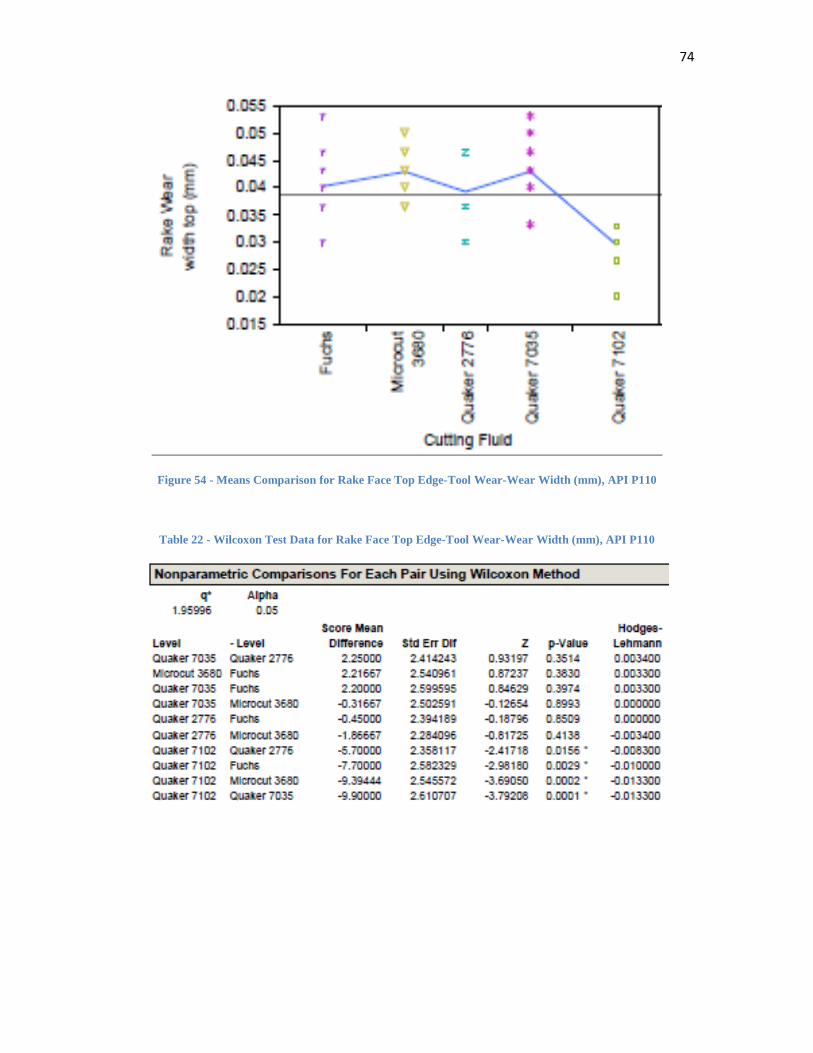
74

Figure 54 - Means Comparison for Rake Face Top Edge-Tool Wear-Wear Width (mm), API P110

Table 22 - Wilcoxon Test Data for Rake Face Top Edge-Tool Wear-Wear Width (mm), API P110

75

Rake Face Leading Edge – Tool Wear – Wear Width

L80 –

Table 23 - Raw Data for Rake Face Leading Edge-Tool Wear-Wear Width (mm), API L80

Figure 55 - Means Comparison for Rake Face Leading Edge-Tool Wear-Wear Width (mm), API L80

Fuchs QC 7102 QC 2776 QC 7035 MC 3680

0.0375 0.0266 0.0300 0.0433 0.0400

0.0266 0.0300 0.0433 0.0333

0.0300 0.0330 0.0333 0.0433 0.0366

0.0300 0.0300 0.0366 0.0433

0.0300 0.0300 0.0400 0.0400 0.0500

0.0400 0.0200 0.0433 0.0400 0.0366

0.0366 0.0367 0.0433 0.0333 0.0466

0.0233 0.0300 0.0333 0.0466 0.0500

0.0366 0.0300 0.0400 0.0300

0.0266 0.0330 0.0433 0.0400

76

Table 24 - Wilcoxon Test Data for Rake Face Leading Edge-Tool Wear-Wear Width (mm), API L80

P110 –

Table 25 - Raw Data for Rake Face Leading Edge-Tool Wear-Wear Width (mm), API P110

Fuchs QC 7102 QC 2776 QC 7035 MC 3680

0.0233 0.0300 0.0300 0.0400 0.0366

0.0330 0.0300 0.0300 0.0333 0.0366

0.0330 0.0200 0.0366 0.0433 0.0400

0.0300 0.0233 0.0330 0.0400 0.0366

0.0366 0.0233 0.0366 0.0400 0.0330

0.0233 0.0266 0.0366 0.0266

0.0300 0.0233 0.0366 0.0330

0.0166 0.0266 0.0400 0.0266

0.0200 0.0167 0.0400

0.0266 0.0266 0.0400 0.0266

77

Figure 56 - Means Comparison for Rake Face Leading Edge-Tool Wear-Wear Width (mm), API P110

Table 26 - Wilcoxon Test Data for Rake Face Leading Edge-Tool Wear-Wear Width (mm), API P110

78

Rake Face Trailing Edge – Tool Wear – Wear Width

L80 –

Table 27 - Raw Data for Rake Face Trailing Edge-Tool Wear-Wear Width (mm), API L80

Figure 57 - Means Comparison for Rake Face Trailing Edge-Tool Wear-Wear Width (mm), API L80

Fuchs QC 7102 QC 2776 QC 7035 MC 3680

0.0330 0.0433 0.0400 0.0433 0.0333

0.0366 0.0333 0.0466 0.0400

0.0366 0 0.0333 0.0366 0.0400

0.0233 0.0400 0.0333 0.0366

0.0433 0.0266 0.0366 0.0400 0.0366

0.0500 0.0200 0.0366 0.0466 0.0400

0.0333 0 0.0400 0.0333 0.0533

0.0333 0 0.0400 0.0300 0.0400

0.0466 0.0300 0.0200 0.0366

0.0300 0.0300 0.0300 0.0366

79

Table 28 - Wilcoxon Test Data for Rake Face Trailing Edge-Tool Wear-Wear Width (mm), API L80

P110 –

Table 29 - Raw Data for Rake Face Trailing Edge-Tool Wear-Wear Width (mm), API P110

Fuchs QC 7102 QC 2776 QC 7035 MC 3680

0.0233 0 0.0300 0.0330 0.0466

0.0366 0 0.0300 0.0500 0.0400

0.0400 0 0.0333 0.0330 0.0330

0.0400 0.0266 0.0400 0.0400 0.0366

0.0433 0 0.0366 0.0500 0.0400

0.0366 0 0.0500 0.0366

0.0333 0 0.0333 0.0366

0.0366 0 0.0266 0.0333

0.0400 0.0266 0.0266

0.0333 0 0.0300 0.0400

80

Figure 58 - Means Comparison for Rake Face Trailing Edge-Tool Wear-Wear Width (mm), API P110

Table 30 - Wilcoxon Test Data for Rake Face Trailing Edge-Tool Wear-Wear Width (mm), API P110

81

Rake Face – Tool Wear - Crater Area

L80 –

Table 31 - Raw Data for Rake Face-Tool Wear-Crater Area (mm^2), API L80

Figure 59 - Means Comparison for Rake Face-Tool Wear-Crater Area (mm^2), API L80

Fuchs QC 7102 QC 2776 QC 7035 MC 3680

0.0200 0 0 0 0

0.0050 0 0 0

0 0 0 0 0

0 0 0 0

0.0200 0 0 0 0

0 0 0 0 0

0 0 0 0 0

0.0026 0 0 0 0

0 0 0 0

0 0.0300 0 0

82

Table 32 - Wilcoxon Test Data for Rake Face-Tool Wear-Crater Area (mm^2), API L80

P110 -

Table 33 - Raw Data for Rake Face-Tool Wear-Crater Area (mm^2), API P110

Fuchs QC 7102 QC 2776 QC 7035 MC 3680

0 0 0 0 0

0 0 0 0 0

0 0 0 0 0

0 0 0 0 0

0.040 0 0 0 0

0 0 0 0

0 0 0 0

0 0 0 0

0 0 0

0 0 0 0

83

Figure 60 - Means Comparison for Rake Face-Tool Wear-Crater Area (mm^2), API P110

Table 34 - Wilcoxon Test Data for Rake Face-Tool Wear-Crater Area (mm^2), API P110

84

Rake Face Leading Edge – Coating Wear – Wear Width

L80 –

Table 35 - Raw Data for Rake Face Leading Edge-Coating Wear-Wear Width (mm), API L80

Figure 61- Means Comparison for Rake Face Leading Edge-Coating Wear-Wear Width (mm), API L80

Fuchs QC 7102 QC 2776 QC 7035 MC 3680

0.2000 0 0 0 0

0.1966 0 0 0

0.1866 0 0.0933 0 0

0 0.1100 0 0

0.1733 0 0.0966 0.0866 0

0.1866 0 0 0 0

0.1866 0 0 0 0

0.1833 0 0 0 0

0.2200 0 0 0

0.1866 0 0 0

85

Table 36 - Wilcoxon Test Data for Rake Face Leading Edge-Coating Wear-Wear Width (mm), API L80

P110 –

Table 37 - Raw Data for Rake Face Leading Edge-Coating Wear-Wear Width (mm), API P110

Fuchs QC 7102 QC 2776 QC 7035 MC 3680

0.1325 0 0.1666 0.1100 0.0866

0.1266 0.1000 0.0933 0.0866 0.0933

0.1500 0.0567 0.0966 0.0900 0.1266

0.1200 0.0600 0.1133 0.1033 0.1000

0.1100 0.0700 0.1033 0.1400 0.1266

0.1233 0 0.1033 0.1000

0.1133 0 0.0900 0.1300

0.1033 0 0.1000 0.0866

0.0600 0 0.0933

0.0966 0.0767 0.1366 0.0666

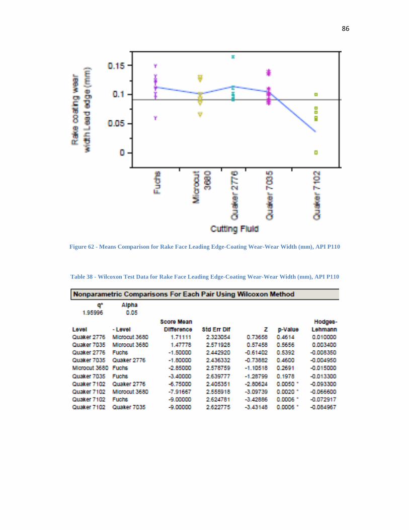
86

Figure 62 - Means Comparison for Rake Face Leading Edge-Coating Wear-Wear Width (mm), API P110

Table 38 - Wilcoxon Test Data for Rake Face Leading Edge-Coating Wear-Wear Width (mm), API P110

87

Rake Face Top Edge – Coating Wear – Wear Width

L80 –

Table 39 - Raw Data for Rake Face Top Edge-Coating Wear-Wear Width (mm), API L80

Figure 63- Means Comparison for Rake Face Top Edge-Coating Wear-Wear Width (mm), API L80

Fuchs QC 7102 QC 2776 QC 7035 MC 3680

0.1400 0 0 0 0

0.1866 0 0 0

0.2033 0 0.1000 0 0

0 0.0866 0 0

0.1933 0 0.0866 0.0900 0

0.2033 0 0 0 0

0.1966 0 0 0 0

0.1800 0 0 0 0

0.1833 0 0 0

0.2066 0 0 0

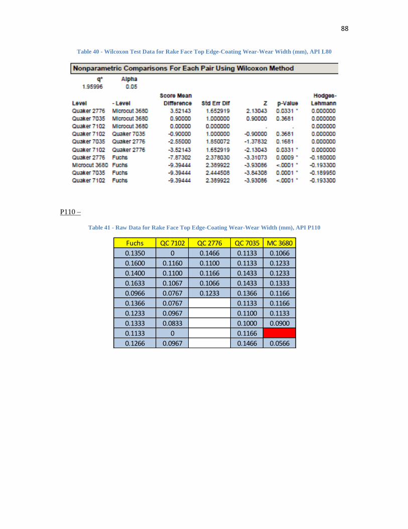
88

Table 40 - Wilcoxon Test Data for Rake Face Top Edge-Coating Wear-Wear Width (mm), API L80

P110 –

Table 41 - Raw Data for Rake Face Top Edge-Coating Wear-Wear Width (mm), API P110

Fuchs QC 7102 QC 2776 QC 7035 MC 3680

0.1350 0 0.1466 0.1133 0.1066

0.1600 0.1160 0.1100 0.1133 0.1233

0.1400 0.1100 0.1166 0.1433 0.1233

0.1633 0.1067 0.1066 0.1433 0.1333

0.0966 0.0767 0.1233 0.1366 0.1166

0.1366 0.0767 0.1133 0.1166

0.1233 0.0967 0.1100 0.1133

0.1333 0.0833 0.1000 0.0900

0.1133 0 0.1166

0.1266 0.0967 0.1466 0.0566

89

Figure 64 - Means Comparison for Rake Face Top Edge-Coating Wear-Wear Width (mm), API P110

Table 42 - Wilcoxon Test Data for Rake Face Top Edge-Coating Wear-Wear Width (mm), API P110

90

Leading Flank – Tool Wear – Wear Area

L80 –

Table 43 - Raw Data for Leading Flank-Tool Wear-Wear Area (mm^2), API L80

Figure 65 - Means Comparison for Leading Flank-Tool Wear-Wear Area (mm^2), API L80

Fuchs QC 7102 QC 2776 QC 7035 MC 3680

0.0400 0.0500 0.0500 0.0500 0.0500

0.0400 0.0400 0.0500 0.0400

0.0500 0.0300 0.0500 0.0500 0.0500

0.0400 0.0500 0.0400 0.0500

0.0500 0.0300 0.0600 0.0500 0.0500

0.0500 0.0400 0.0600 0.0400 0.0500

0.0500 0.0500 0.0400 0.0400 0.0600

0.0400 0.0300 0.0500 0.0400 0.0400

0.0400 0.0400 0.0400 0.0500

0.0400 0.0600 0.0400 0.0400

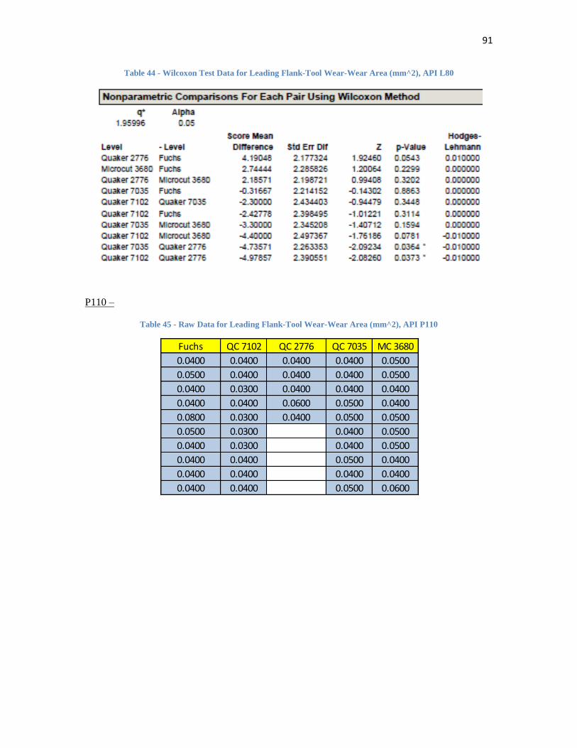
91

Table 44 - Wilcoxon Test Data for Leading Flank-Tool Wear-Wear Area (mm^2), API L80

P110 –

Table 45 - Raw Data for Leading Flank-Tool Wear-Wear Area (mm^2), API P110

Fuchs QC 7102 QC 2776 QC 7035 MC 3680

0.0400 0.0400 0.0400 0.0400 0.0500

0.0500 0.0400 0.0400 0.0400 0.0500

0.0400 0.0300 0.0400 0.0400 0.0400

0.0400 0.0400 0.0600 0.0500 0.0400

0.0800 0.0300 0.0400 0.0500 0.0500

0.0500 0.0300 0.0400 0.0500

0.0400 0.0300 0.0400 0.0500

0.0400 0.0400 0.0500 0.0400

0.0400 0.0400 0.0400 0.0400

0.0400 0.0400 0.0500 0.0600

92

Figure 66 - Means Comparison for Leading Flank-Tool Wear-Wear Area (mm^2), API P110

Table 46 - Wilcoxon Test Data for Leading Flank-Tool Wear-Wear Area (mm^2), API P110

93

Leading Flank – Tool Wear – Wear Width

L80 –

Table 47 - Raw Data for Leading Flank-Tool Wear-Wear Width (mm), API L80

Figure 67 - Means Comparison for Leading Flank-Tool Wear-Wear Width (mm), API L80

Fuchs QC 7102 QC 2776 QC 7035 MC 3680

0.0400 0.0467 0.0466 0.0466 0.0400

0.0366 0.0267 0.0433 0.0330

0.0330 0.0267 0.0466 0.0500 0.0500

0.0330 0.0400 0.0433 0.0433

0.0366 0.0266 0.0500 0.0466 0.0500

0.0400 0.0300 0.0466 0.0366 0.0433

0.0400 0.0300 0.0400 0.0433 0.0500

0.0433 0.0300 0.0500 0.0366 0.0366

0.0366 0.0300 0.0366 0.0400

0.0366 0.0330 0.0333 0.0366

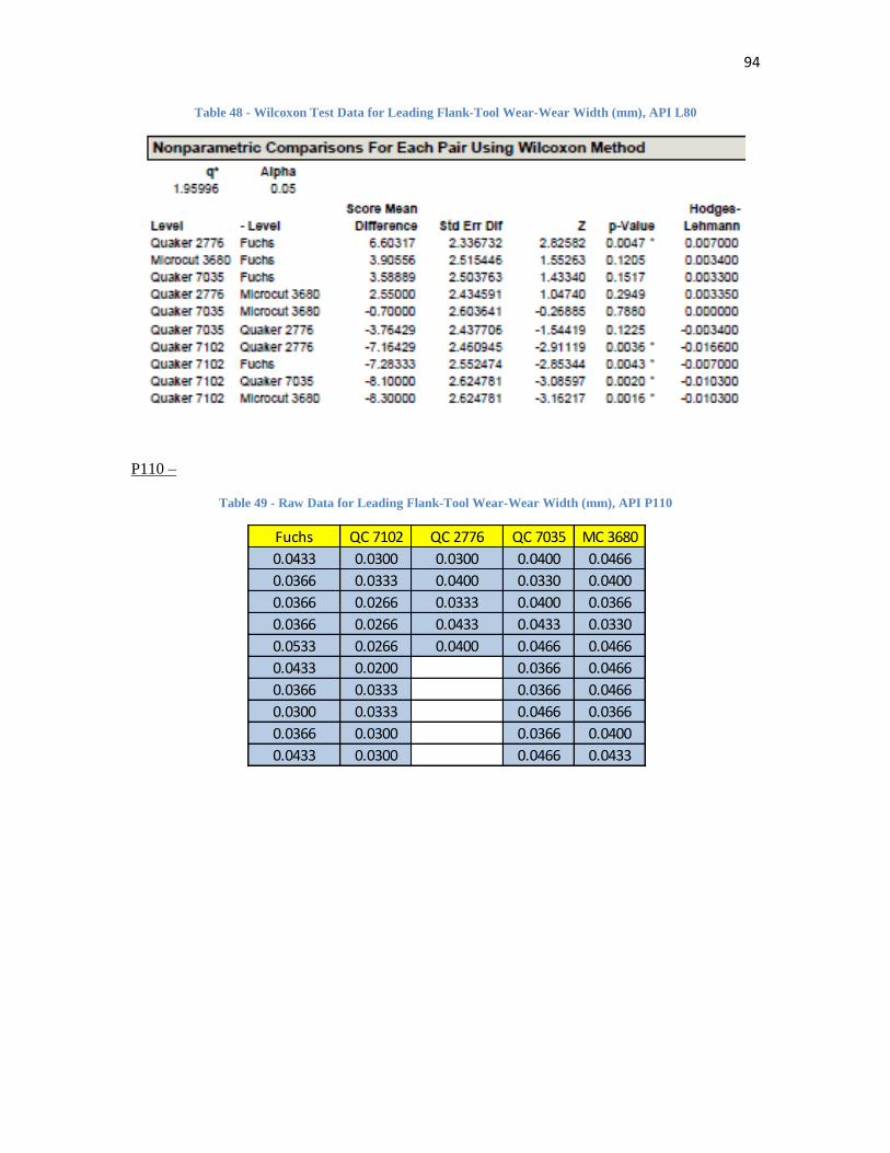
94

Table 48 - Wilcoxon Test Data for Leading Flank-Tool Wear-Wear Width (mm), API L80

P110 –

Table 49 - Raw Data for Leading Flank-Tool Wear-Wear Width (mm), API P110

Fuchs QC 7102 QC 2776 QC 7035 MC 3680

0.0433 0.0300 0.0300 0.0400 0.0466

0.0366 0.0333 0.0400 0.0330 0.0400

0.0366 0.0266 0.0333 0.0400 0.0366

0.0366 0.0266 0.0433 0.0433 0.0330

0.0533 0.0266 0.0400 0.0466 0.0466

0.0433 0.0200 0.0366 0.0466

0.0366 0.0333 0.0366 0.0466

0.0300 0.0333 0.0466 0.0366

0.0366 0.0300 0.0366 0.0400

0.0433 0.0300 0.0466 0.0433

95

Figure 68 - Means Comparison for Leading Flank-Tool Wear-Wear Width (mm), API P110

Table 50 - Wilcoxon Test Data for Leading Flank-Tool Wear-Wear Width (mm), API P110

96

Top Flank – Tool Wear – Wear Width

L80 –

Table 51 - Raw Data for Top Flank-Tool Wear-Wear Width (mm), API L80

Figure 69 - Means Comparison for Top Flank-Tool Wear-Wear Width (mm), API L80

Fuchs QC 7102 QC 2776 QC 7035 MC 3680

0.1300 0.0500 0.0533 0.0500 0.0433

0.1300 0.0367 0.0466 0.0400

0.1133 0.0266 0.0500 0.0466 0.0300

0.0433 0.0400 0.0400 0.0366

0.1400 0.0567 0.0566 0.0400 0.0466

0.1200 0.0000 0.0533 0.0333 0.0300

0.0933 0.0433 0.0400 0.0433 0.0400

0.0966 0.0400 0.0566 0.0400 0.0366

0.1000 0.0500 0.0400 0.0333

0.0833 0.0700 0.0533 0.0366

97

Table 52 - Wilcoxon Test Data for Top Flank-Tool Wear-Wear Width (mm), API L80

P110 –

Table 53 - Raw Data for Top Flank-Tool Wear-Wear Width (mm), API P110

Fuchs QC 7102 QC 2776 QC 7035 MC 3680

0.1200 0.0800 0.0433 0.0566 0.0633

0.1400 0.0933 0.0600 0.0466 0.0566

0.1033 0.0633 0.0600 0.0533 0.0400

0.1133 0.0933 0.0566 0.0533 0.0433

0.1866 0.0500 0.0466 0.0533 0.0400

0.1366 0.0500 0.0566 0.0466

0.1133 0.0700 0.0400 0.0400

0.1100 0.0433 0.0500 0.0466

0.1133 0.0433 0.0566

0.1300 0.0633 0.0700 0.1000

98

Figure 70 - Means Comparison for Top Flank-Tool Wear-Wear Width (mm), API P110

Table 54 - Wilcoxon Test Data for Top Flank-Tool Wear-Wear Width (mm), API P110

99

Top Flank – Tool Wear – Wear Area

L80 –

Table 55 - Raw Data for Top Flank-Tool Wear-Wear Area (mm^2), API L80

Figure 71 - Means Comparison for Top Flank-Tool Wear-Wear Area (mm^2), API L80

Fuchs QC 7102 QC 2776 QC 7035 MC 3680

0.1300 0.0700 0.0500 0.0600 0.0500

0.1000 0.0500 0.0500 0.0500

0.1100 0.0300 0.0500 0.0500 0.0400

0.0500 0.0500 0.0400 0.0500

0.1200 0.0700 0.0500 0.0500 0.0400

0.1200 0.0300 0.0600 0.0400 0.0500

0.1000 0.0400 0.0600 0.0500 0.0400

0.1000 0.0500 0.0600 0.0400 0.0400

0.1100 0.0700 0.0400 0.0500

0.1000 0.1100 0.0600 0.0500

100

Table 56 - Wilcoxon Test Data for Top Flank-Tool Wear-Wear Area (mm^2), API L80

P110 –

Table 57 - Raw Data for Top Flank-Tool Wear-Wear Area (mm^2), API P110

Fuchs QC 7102 QC 2776 QC 7035 MC 3680

0.1300 0.0900 0.0400 0.0600 0.0700

0.1200 0.1000 0.0700 0.0500 0.0600

0.0900 0.0700 0.0600 0.0600 0.0500

0.1200 0.1100 0.0700 0.0500 0.0500

0.2900 0.0500 0.0500 0.0500 0.0500

0.1200 0.0600 0.0600 0.0500

0.1100 0.0800 0.0600 0.0500

0.1000 0.0600 0.0500 0.0600

0.1100 0.0400 0.0500

0.1200 0.0800 0.0600 0.1100

101

Figure 72 - Means Comparison for Top Flank-Tool Wear-Wear Area (mm^2), API P110

Table 58 - Wilcoxon Test Data for Top Flank-Tool Wear-Wear Area (mm^2), API P110

102

APPENDIX C – EXAMPLE PICTURES SHOWING THREAD WEAR

Figure 73 - A Chipped Rake Face of an Insert Used to Machine API L80 with EcoCool

Figure 74 – An Insert that was used to Machine API L80 with QC7035

103

Figure 75 – An Insert that was Chipped while Machining API P110 with MC3680

Figure 76 - Leading Flank of an Insert that was used to Machine API P110 with QC7102

104

Figure 77 – Top Flank of an Insert that was used to Machine API L80 with QC2776

105

REFERENCES

1. International Organization for Standardization. Tool-life testing with single-point

turning tools, 1993. ISO 3685.

2. L. De Chiffre (I), W. Belluco. Comparison of Methods for Cutting Fluid

Performance Testing Annals of the CIRP Vol. 49/1/2000

3. Wisley Falco Sales, Anselmo Eduardo Diniz and Álisson Rocha Machado.

Application of Cutting Fluids in Machining Processes. Journal of the Brazilian

Society of Mechanical Sciences

Print version ISSN 0100-7386

J. Braz. Soc. Mech. Sci. vol.23 no.2 Rio de Janeiro 2001

4. Dwight V. Squire, Chol K. Syn and Bradely L. Fix. Machinability. Study of

Aermet 100. Manufacturing and Materials Engineering Division, Lawrence

Livermore National Laboratory, Livermore CA 94550.

5. M. Kious, A. Ouahabi, M. Boudraa, R. Serra, A. Cheknane. Detection process

approach of tool wear in high speed milling Measurement 43 (2010) 1439–1446

6. Viktor P. Astakhov. The assessment of cutting tool wear. International journal of

machine tool & manufacture. November 2003

7. JMP 9.0.0, copyright 2010 SAS Institute Inc.

8. Erik Oberg, Franklin D. Jones, Holbrook L. Horton, Henry H. Ryffel. Robert E.

Green. Machinery‘s Handbook, 24th edition. 1991

9. Dragos A. Axinte, Walter Belluco, Leonardo De Chiffre. Reliable tool life

measurements in turning — an application to cutting fluid efficiency evaluation

International Journal of Machine Tools & Manufacture 41 (2001) 1003–1014

10. W. K. Mook & H. H. Shahabi & M. M. Ratnam. Measurement of nose radius wear

in turning tools from a single 2D image using machine vision Int J Adv Manuf

Technol (2009) 43:217–225

11. J. Jurkovic, M. Korosec, J. Kopac. New approach in tool wear measuring

technique using CCD vision system International Journal of Machine Tools &

Manufacture 45 (2005) 1023–1030

12. G. Byrne, D. Dornfeld, I. lnasaki, G. Ketteler, W. Konig and R. Teti. Tool

Condition Monitoring (TCM) - The Status quo and Industrial Application Research

Annals of the CIRP Vol. 44/2/1995

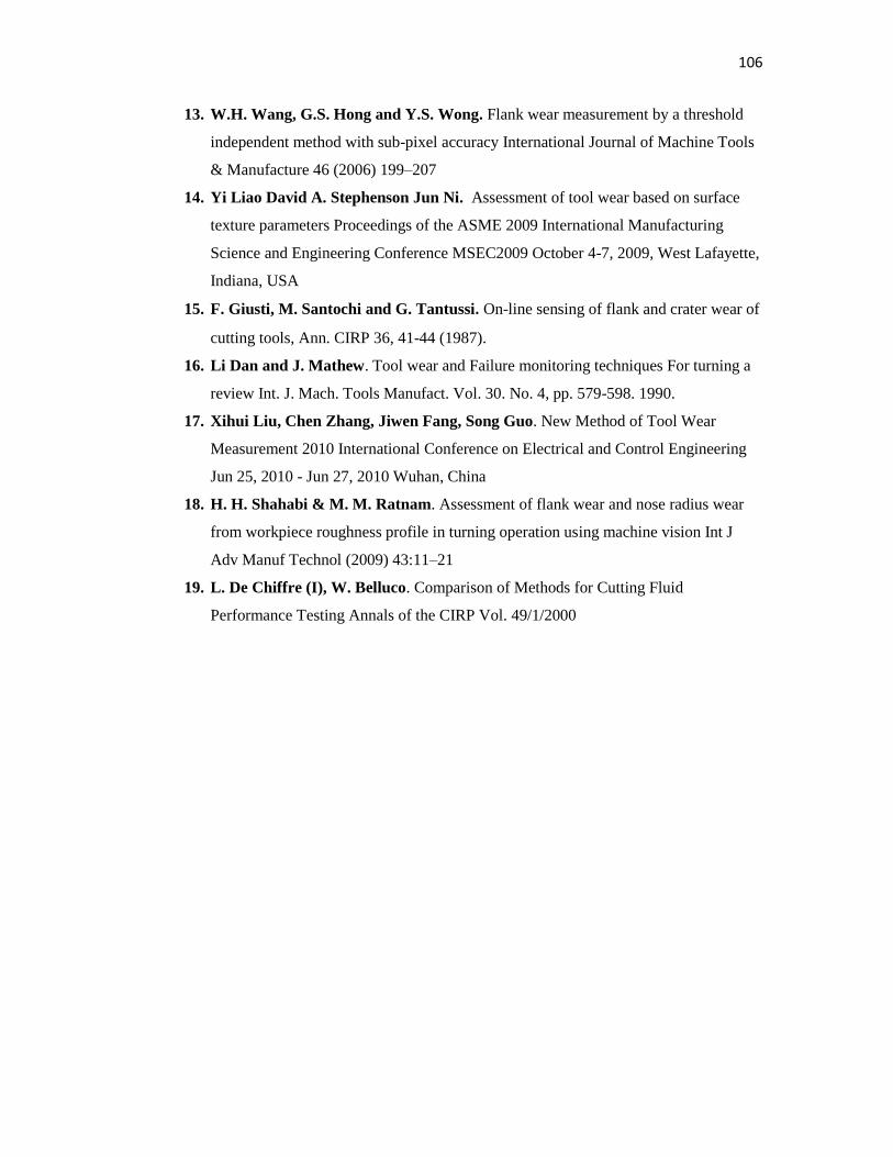
106

13. W.H. Wang, G.S. Hong and Y.S. Wong. Flank wear measurement by a threshold

independent method with sub-pixel accuracy International Journal of Machine Tools

& Manufacture 46 (2006) 199–207

14. Yi Liao David A. Stephenson Jun Ni. Assessment of tool wear based on surface

texture parameters Proceedings of the ASME 2009 International Manufacturing

Science and Engineering Conference MSEC2009 October 4-7, 2009, West Lafayette,

Indiana, USA

15. F. Giusti, M. Santochi and G. Tantussi. On-line sensing of flank and crater wear of

cutting tools, Ann. CIRP 36, 41-44 (1987).

16. Li Dan and J. Mathew. Tool wear and Failure monitoring techniques For turning a

review Int. J. Mach. Tools Manufact. Vol. 30. No. 4, pp. 579-598. 1990.

17. Xihui Liu, Chen Zhang, Jiwen Fang, Song Guo. New Method of Tool Wear

Measurement 2010 International Conference on Electrical and Control Engineering

Jun 25, 2010 - Jun 27, 2010 Wuhan, China

18. H. H. Shahabi & M. M. Ratnam. Assessment of flank wear and nose radius wear

from workpiece roughness profile in turning operation using machine vision Int J

Adv Manuf Technol (2009) 43:11–21

19. L. De Chiffre (I), W. Belluco. Comparison of Methods for Cutting Fluid

Performance Testing Annals of the CIRP Vol. 49/1/2000

http://www.sciencedirect.com/science?_ob=RedirectURL&_method=outwardLink&_partnerName=27983&_origin=article&_zone=art_page&_linkType=scopusAuthorDocuments&_targetURL=http%3A%2F%2Fwww.scopus.com%2Fscopus%2Finward%2Fauthor.url%3FpartnerID%3D10%26rel%3D3.0.0%26sortField%3Dcited%26sortOrder%3Dasc%26author%3DGiusti,%2520F.%26authorID%3D7006275198%26md5%3D81cfde32211e98d0d4bd8b0a2b8ff4cf&_acct=C000004038&_version=1&_userid=32321&md5=5690b36fc9917f67283a390b3c45abcd

http://www.sciencedirect.com/science?_ob=RedirectURL&_method=outwardLink&_partnerName=27983&_origin=article&_zone=art_page&_linkType=scopusAuthorDocuments&_targetURL=http%3A%2F%2Fwww.scopus.com%2Fscopus%2Finward%2Fauthor.url%3FpartnerID%3D10%26rel%3D3.0.0%26sortField%3Dcited%26sortOrder%3Dasc%26author%3DSantochi,%2520M.%26authorID%3D6701580653%26md5%3Dcecdb1e07e89013d74753faef6e5eb97&_acct=C000004038&_version=1&_userid=32321&md5=4b95b9d9e8a8e23acf7b8a55c0231828

http://www.sciencedirect.com/science?_ob=RedirectURL&_method=outwardLink&_partnerName=27983&_origin=article&_zone=art_page&_linkType=scopusAuthorDocuments&_targetURL=http%3A%2F%2Fwww.scopus.com%2Fscopus%2Finward%2Fauthor.url%3FpartnerID%3D10%26rel%3D3.0.0%26sortField%3Dcited%26sortOrder%3Dasc%26author%3DTantussi,%2520G.%26authorID%3D6603307393%26md5%3D247ded728d9ac7075a0c5bc91845b882&_acct=C000004038&_version=1&_userid=32321&md5=6646b6ae23f6c40239d33216b3ca5ec2