L

An Investigation of the Tensile Strength and Stiffness of UnidirectionalPolymer-Matrix, Carbon-Fiber Composites under the Influence of Elevated

Temperatures

ByBrady M. Walther

Thesis submitted to the Faculty of theVirginia Polytechnic Institute and State University

in Partial fulfillment of the requirements for the degree ofMaster of Science

InEngineering Mechanics

APPROVED

______________________________________Ken Reifsnider, Chairman

____________________________ __________________________John J. Lesko David Gao

May 27, 1998Blacksburg, Virginia

LL

An investigation of the Tensile Strength and Stiffness of UnidirectionalPolymer-Matrix, Carbon-Fiber Composites under the Influence of Elevated

TemperaturesBy

Brady M. Walther

(ABSTRACT)

Traditionally it was thought that the unidirectional strength in the fiber direction

of fiber dominated composites was not influenced by the matrix material. As long as the

fiber was not affected then the strength would remain. However this thesis will challenge

that belief. The unidirectional strength in the fiber direction of fiber dominated

composites is influenced by the matrix material.

Currently some companies in the industry that design with polymer-carbon fiber

composites use a "knock down" factor on mechanical properties to account for the effect

of environment or elevated temperatures. For example, the failure strength of a

composite is reduced by some arbitrary factor such as ten percent for the adverse

environmental condition that the system will encounter. If the composite must operate at

elevated temperatures, then the design failure strength will reflect this condition with

some arbitrary reduction. This reduction may be too aggressive or not aggressive enough

for some composite systems and conditions, and does not reflect the details of the

material or the situation.

To avoid grossly over or under designing with a "knock down" factor, many

companies will invest money and time to determine the macro-mechanical response of a

particular composite system under the expected service conditions. This is a large

LLL

investment because every specific material and each new system that is considered must

be tested. However, if a general understanding of the effect of elevated temperatures on

the tensile strength of polymer-carbon fiber composites can be developed, then this will

save money and time because the physics and mechanics can be applied independently

for all specific matrix materials and conditions.

This study investigated the micro-mechanical constituent properties that were

thought to be affected by elevated temperatures. Then micro-mechanical equations were

changed to reflect this effect and used to calculate the macro-mechanical tensile strength

of the composite. These predictions were compared with macro-mechanical tensile

strength data obtained under the influence of elevated temperatures. The composite

systems in this study were unidirectional continuous carbon fibers in a polymer matrix.

The object of this study was to examine the quasi-static tensile strength of

unidirectional polymer composites, and then use current analytic models to predict the

experimental results. The strength and stiffness properties were measured in different

temperature environments. The temperature environments ranged from -184.4 degrees

Celsius to 220 degrees Celsius. New arguments were added to the current models to

express the physics and mechanics of the tensile strength problem at different

temperatures. The macro-mechanical and micro-mechanical effects were studied with

different composite systems. However, all the systems had polymer matrixes with carbon

fibers. The different matrix materials were polyphenylene sulfide (PPS), vinyl ester with

two different fiber-matrix interface materials, and polyether ether ketone (PEEK). The

different material systems were examined for comparisons to analytic models and to add

to the database for these material systems.

LY

As much information was obtained about the processing procedures of each of the

material systems as possible. Then mechanical tests were preformed to determine the

temperature response of the strength and stiffness of each material system. Finial

observations were made about the behavior of material systems.

Current research and development has produced models for the prediction of the

strength of unidirectional composites. These models are essential for the design and use

for these types of material in the industry. The current micro-mechanical models

describe the strength of a unidirectional polymer composite in the tensile direction.

However, these models do not explicitly account for different temperature environments.

Therefore, the models were developed to include the effect of elevated temperature on

strength.

Y

ACKNOWLEDGMENTS

The author would like to thank the following people for their involvement to this work:

• Dr. Ken L. Reifsnider, for all of the time and support he spent on this project. He is a

true inspiration and role model for all young engineers.

• Dr. David Gao and Dr. John Lesko, for serving as committee members and for

helping to edit this document.

• Dr. Scott Case, for all of his time and effort helping this work become complete.

• National Science Foundation and the Air Force, for the funding of this work and the

educational opportunity.

• Members of the MRG at Virginia Tech, for the support and help in the lab.

• Mac McCord, for all the days that the lab equipment needed setting up.

• Danny Reed, for the open use of the fabrication lab.

• Shelia Collins, for the know how of getting things done under pressure.

• The authors parents, for all their help in keeping things possible.

YL

Table of Content

List of Tables ......................................................................................................viii

List of Figures ........................................................................................................ x

I. Introduction and Literature Review................................................................ 1Literature Review.................................................................................................... 3

Strength ....................................................................................................... 3General Formulation of Strength Models.................................................... 5Model One................................................................................................... 5Model Two ................................................................................................ 17Quantitative Differences between the Models .......................................... 25Temperature Effects on the Strength......................................................... 25Interfacial Shear Strength at Elevated Temperatures ................................ 30Bulk Polymer Stiffness at Elevated Temperatures.................................... 33Mechanical Properties for Materials ......................................................... 33

II. Experimental Procedures .............................................................................. 35General Equipment................................................................................................ 35

XPS ........................................................................................................... 35Fiber Volume Fraction Analysis ............................................................... 36C-Scans...................................................................................................... 36DMA.......................................................................................................... 37Quasi-static Tension Macro-Mechanical Test........................................... 37

Materials................................................................................................................ 39Polyphenylene Sulfide (PPS) Composite.................................................. 39General Description................................................................................... 39Processing.................................................................................................. 40Specimen Preparation................................................................................ 40Vinyl Ester Composite .............................................................................. 42General Description................................................................................... 42Processing.................................................................................................. 43Specimen Preparation................................................................................ 43Polyether Ether Ketone (PEEK ) Composite ............................................ 44General Description................................................................................... 44Processing.................................................................................................. 45Specimen Preparation................................................................................ 45

YLL

III. Experimental Results and Discussion......................................................... 48Polyphenylene Sulfide (PPS) Composite.................................................. 48Fiber Volume Fracture .............................................................................. 48XPS ........................................................................................................... 48DMA.......................................................................................................... 49Results of Macro-Mechanical Test ........................................................... 50Fracture Modes.......................................................................................... 59Vinyl Ester................................................................................................. 61Fiber Volume Fracture .............................................................................. 61Results of Macro-Mechanical Test ........................................................... 62Fracture Modes.......................................................................................... 69PEEK......................................................................................................... 74Fiber Volume Fracture .............................................................................. 74Results of Macro-Mechanical Test ........................................................... 75Fracture Modes.......................................................................................... 83Summary of Experimental Results............................................................ 83

IV. Model Development and Prediction of Experimental Results.................. 85Parametric Study ....................................................................................... 85Changes to Model Parameters for Elevated Temperature......................... 86Model Predictions of Strength at Elevated Temperature .......................... 90

V. Summary, Conclusions, and Future Work .................................................. 95Summary of Method.................................................................................. 95Conclusions ............................................................................................... 95Future Work .............................................................................................. 96

References .......................................................................................................... 100

Appendix A: PPS RAW DATA........................................................................ 102

Appendix B: PEEK RAW DATA .................................................................... 108

Appendix C: VINYL ESTER RAW DATA.................................................... 110

VITA ................................................................................................................. 112

YLLL

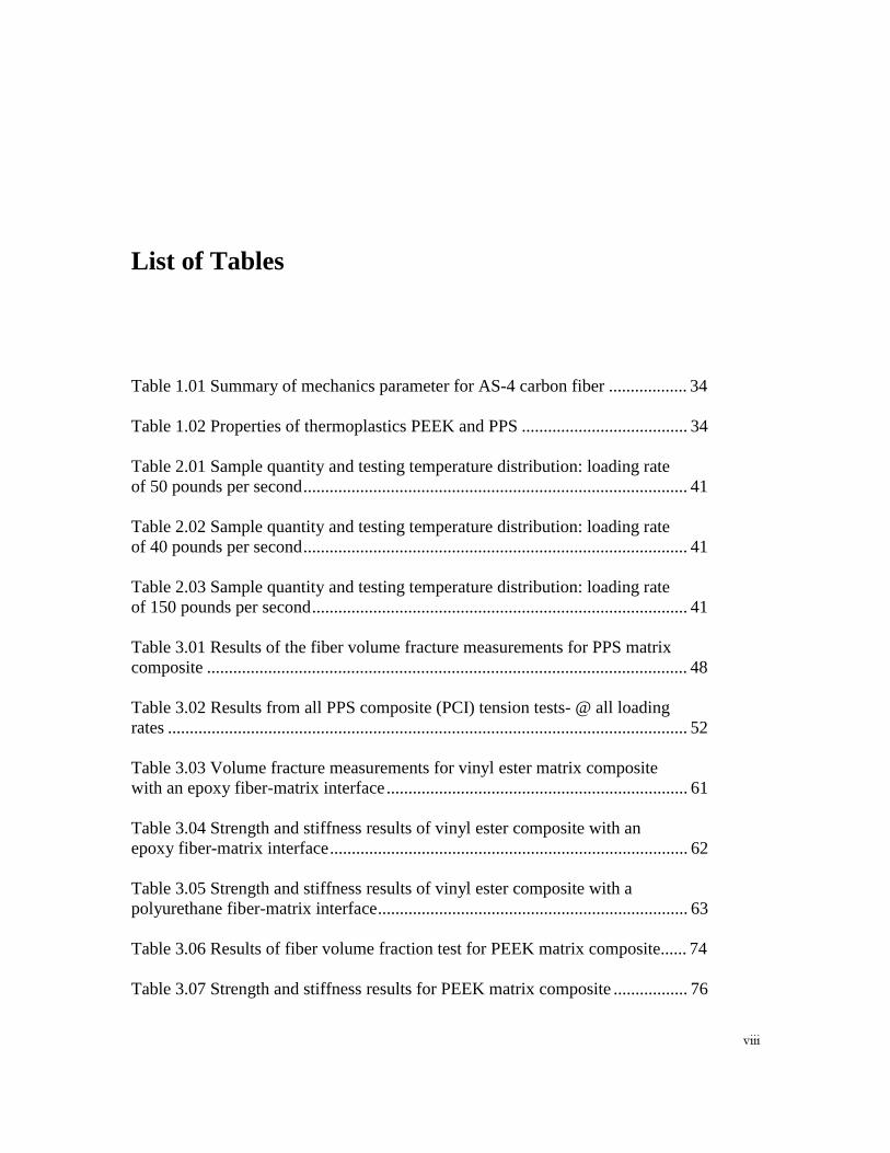
List of Tables

Table 1.01 Summary of mechanics parameter for AS-4 carbon fiber .................. 34

Table 1.02 Properties of thermoplastics PEEK and PPS ...................................... 34

Table 2.01 Sample quantity and testing temperature distribution: loading rateof 50 pounds per second........................................................................................ 41

Table 2.02 Sample quantity and testing temperature distribution: loading rateof 40 pounds per second........................................................................................ 41

Table 2.03 Sample quantity and testing temperature distribution: loading rateof 150 pounds per second...................................................................................... 41

Table 3.01 Results of the fiber volume fracture measurements for PPS matrixcomposite .............................................................................................................. 48

Table 3.02 Results from all PPS composite (PCI) tension tests- @ all loadingrates ....................................................................................................................... 52

Table 3.03 Volume fracture measurements for vinyl ester matrix compositewith an epoxy fiber-matrix interface..................................................................... 61

Table 3.04 Strength and stiffness results of vinyl ester composite with anepoxy fiber-matrix interface.................................................................................. 62

Table 3.05 Strength and stiffness results of vinyl ester composite with apolyurethane fiber-matrix interface....................................................................... 63

Table 3.06 Results of fiber volume fraction test for PEEK matrix composite...... 74

Table 3.07 Strength and stiffness results for PEEK matrix composite ................. 76

L[

Table 4.01 Input variables for the micro-mechanical models for PPScomposite .............................................................................................................. 91

Table 4.02 Input variables for the micro-mechanical models for PEEKcomposite .............................................................................................................. 91

Table 4.03 Model strength results for the PPS composite system ........................ 92

Table 4.04 Model strength results for the PEEK composite system..................... 92

[

List of Figures

Figure 1.01 Batdorf Q-plot where composite failure occurs at the point ofinstability................................................................................................................. 8

Figure 1.02 Fiber fracture of unidirectional composites used by Gao andReifsnider .............................................................................................................. 10

Figure 1.03 Schematic of concentric cylinder model with a core of brokenfibers with the neighboring fibers ......................................................................... 18

Figure 1.04 Tensile strength as a function of local ineffective length .................. 28

Figure 1.05 Unidirectional tensile strength as a function of temperature fortwo polymer carbon fiber composites ................................................................... 29

Figure 1.06 Interfacial shear strength as a function of temperature from singlefragmentation test/ Epon 828 DU-700 .................................................................. 32

Figure 1.07 Interfacial shear strength as a function of temperature from singlefragmentation test/ Epon 828 mPDA .................................................................... 32

Figure 1.08 Bulk Epon 828 stress-strain curves at elevated temperatures............ 33

Figure 2.01 MTS with heater box set up with a specimen.................................... 38

Figure 2.02 Cryogenic chamber for quasi-static tension test ................................ 39

Figure 2.03 Drawing of a typical test specimens for PPS system......................... 42

Figure 2.04 Drawing of a typical test specimen for vinyl ester system ................ 44

Figure 2.05 Processing diagram for PEEK composite.......................................... 45

Figure 2.06 Dimensional drawling of PEEK specimens....................................... 46

Figure 2.07 Photograph of PEEK specimens illustrating end tabs,extensometer tabs, and strain gage placement ...................................................... 47

[L

Figure 3.01 DMA Result for PPS matrix composite system................................. 49

Figure 3.02 Stress-strain calibration of extensometer with strain gage strainmeasurements ........................................................................................................ 51

Figure 3.03 Stress-strain curve for PPS composite material ................................. 52

Figure 3.04 A plot of the strength values for the PPS composite material withtheir respective temperatures with standard deviations as error bars.................... 53

Figure 3.05 Young’s modulus for PPS composite system with all loading rates .. 54

Figure 3.06 A bar graph of the strength of PPS Composite (same data thatmakes up Figure 3.04)........................................................................................... 55

Figure 3.07 A bar graph of Young’s modulus for the PPS carbon fibercomposite .............................................................................................................. 55

Figure 3.08 The strength of PPS composite differentiating load rates of 40,50,and 150 pounds per sec ......................................................................................... 56

Figure 3.09 All strength data on PPS composite, data without strainmeasurements ........................................................................................................ 57

Figure 3.10 A family of stress-strain curves for PPS composites at fourdifferent temperatures (30, 90, 110, and 130 degrees Celsius) ............................. 58

Figure 3.11 Strength of PPS composite at elevated temperatures and cryogenictemperatures .......................................................................................................... 59

Figure 3.12 Fracture of PPS specimen at 31.1 degrees Celsius (Front and SideViews) ................................................................................................................... 60

Figure 3.13 Fracture of PPS specimen at 229 degrees Celsius (Front and SideViews) ................................................................................................................... 61

Figure 3.14 Stress-strain curve for vinyl ester with polyurethane interface ......... 63

Figure 3.15 Stress-strain curve for vinyl ester with epoxy interface .................... 64

Figure 3.16 Strength of vinyl ester composite as a function of temperature andtwo different interfaces.......................................................................................... 65

Figure 3.17 Stiffness of vinyl ester composite as a function of temperature andtwo different interfaces.......................................................................................... 66

[LL

Figure 3.18 A family of stress-strain curves for vinyl ester composite with anepoxy fiber-matrix interface at different temperatures (90, 140,35,110, and130 Degrees C)...................................................................................................... 67

Figure 3.19 Strength for vinyl ester composite with both interfaces at elevatedtemperatures and cryogenic temperatures ............................................................. 68

Figure 3.20 Stiffness values of the vinyl ester composite with both fiber-matrix interfaces at elevated temperature and cryogenic temperatures ................ 69

Figure 3.21 Fracture of a vinyl ester specimen with polyurethane fiber-matrixinterface at 33.4 degrees Celsius (Front and Side Views)..................................... 70

Figure 3.22 Fracture of a vinyl ester specimen with polyurethane fiber-matrixinterface at 149.7 degrees Celsius (Front and Side Views)................................... 71

Figure 3.23 Fracture of a vinyl ester specimen with polyurethane fiber-matrixinterface at -184.4 degrees Celsius (Front and Side Views) ................................. 72

Figure 3.24 Fracture of a vinyl ester specimen with epoxy fiber-matrixinterface at 35 degrees Celsius (Front and Side Views)........................................ 73

Figure 3.25 Fracture of a vinyl ester specimen with epoxy fiber-matrixinterface at 140 degrees Celsius (Front and Side Views)...................................... 74

Figure 3.26 C-Scan of PEEK matrix composite ................................................... 75

Figure 3.27 Stress-strain curve for PEEK matrix composite at 150 degrees C .... 77

Figure 3.28 Stress-strain curve of a PEEK matrix composite at 100 degrees C ... 77

Figure 3.29 Stress-strain curve for PEEK matrix composite at 27 degrees C ...... 78

Figure 3.30 A family of stress-strain curves for PEEK matrix at differenttemperatures (27, 90, and 170 Degrees C) ............................................................ 78

Figure 3.31 Strength values of PEEK matrix composite at elevatedtemperatures .......................................................................................................... 80

Figure 3.32 Stiffness values for PEEK matrix composite measured with anextensometer.......................................................................................................... 80

Figure 3.33 Stiffness of PEEK matrix composite measured with a strain gage.... 81

[LLL

Figure 3.34 Average strength of PEEK matrix composite with standarddeviations .............................................................................................................. 82

Figure 3.35 Stiffness of PEEK matrix composite with standard deviations ......... 82

Figure 4.01 Parametric study of the interfacial shear strength effect onstrength of a composite ......................................................................................... 86

Figure 4.02 Approximation of the interfacial shear strength as a function oftemperature for a PPS composite system .............................................................. 87

Figure 4.03 Approximation of the shear modulus as a function of temperaturefor the PPS matrix ................................................................................................. 88

Figure 4.04 Approximation to the interfacial shear strength as a function oftemperature for PEEK composite system.............................................................. 89

Figure 4.05 Approximation of the shear modulus for PEEK as a function oftemperature............................................................................................................ 90

Figure 4.06 Experimental data for PPS compared to model predictions ofstrength .................................................................................................................. 92

Figure 4.07 Experimental data for PEEK composite compared to modelpredictions of strength........................................................................................... 94

Figure 5.01 Processing for 350 degrees F cure cycle for toughened epoxy.......... 98

Figure 5.02 Processing for 250 degrees F cure cycle for toughened epoxy.......... 99

�

I. Introduction and Literature Review

In the past decade polymer based composites have provided a high strength to

weight ratio. Many applications in the aerospace industry have benefited from these

materials. However, in many cases the majority of the material has been placed in the

structures as non-load-bearing members. In order to use composite materials as load-

bearing members, the design parameters must be fully described. This description is very

complex because of the nature of the composite system. Unlike steel or alloys, a

composite system is anisotropic and heterogeneous material. In addition, the properties

are sensitive to environmental conditions such as humidity, temperature, loading rates

and aging.

However, much has been done in the area of describing such materials for design.

One of the most important parameters for design is strength. This is generally defined by

the condition where the material experiences a load and completely fails or fractures

under that load. The micro-mechanics of this failure can be described to predict to the

macro-mechanical failure strength. Two particular micro-mechanical models are

described below. This paper focuses on the strength of composite systems under the

effect of elevated temperature. In addition to strength, the stiffness of the system was

�

measured at elevated temperatures. The effects on the stiffness will be reported;

however, the main focus was on the strength.

The literature review of this paper is intended to give the reader a general

understanding of the strength of unidirectional composites. The major portion of the

review describes the mathematical models used to predict the tensile strength of a

composite system. These are not the only micro-mechanical models that exist.

These models evaluate the system at the micro-mechanical level, unlike

traditional classical laminate theory. Some background information is given about the

philosophy behind the models. However the background information is not extensive.

This thesis focuses on using the existing models and comparing them to experimental

data. The fundamental mathematics will not be changed in the models. However, the

mathematical parameters, that are expected to be affected by elevated temperatures, will

be developed to reflect this change.

The reporting of the experimental work will follow the literature review. Not

only will these data serve to explore the theoretical models but will also add to the library

of data for polymer composites and environmental effects. The next section is the

development of the micro-mechanical models to allow for elevated temperatures in

predicting strength. The micro-mechanical parameters are developed for the effect of

elevated temperatures and strength predictions are made with these developments. The

predictions are compared to the experimental data to test their validity.

�

Literature Review

Strength

Micro-mechanics models have evolved to predict the tensile strength of

unidirectional composites. For the past two decades several researchers have studied

tensile failure and strength. Weibull used the weakest link theory to predict the fracture

of a single fiber. This theory was developed because Weibull discovered that the tensile

strength of a single fiber was not uniform from point to point. Coleman, Rosen, and

Hahn studied the fracture of a bundle of fibers [1]. Rosen calculated the bundle strength

assuming that the statistical distribution of strength of the fibers governs the failure of

each fiber. Therefore, the failure of the bundle of fibers is due to the statistical

accumulation of fiber fractures in the system.

Zweben and Rosen related the failure of the fiber bundles in the company of the

matrix material. They used the ineffective length to estimate the tensile strength. This

was based on shear lag analysis. However, this model did not consider the effects of

stress concentrations in the fibers adjacent to the broken fiber [1].

Batdorf showed that the stress concentrations in the adjacent fiber would lead to

the accumulation of fiber fractures and this would lead to final (ultimate) failure of the

composite [1]. His model uses the argument of the accumulation of a critical number of

fiber fractures called “i-plets” leads to instability. The load level at which the instability

occurs is the failure strength of the laminate.

These models lead us to the point that tensile strength of unidirectional

composites is based on the ineffective length and stress concentration effects near fiber

�

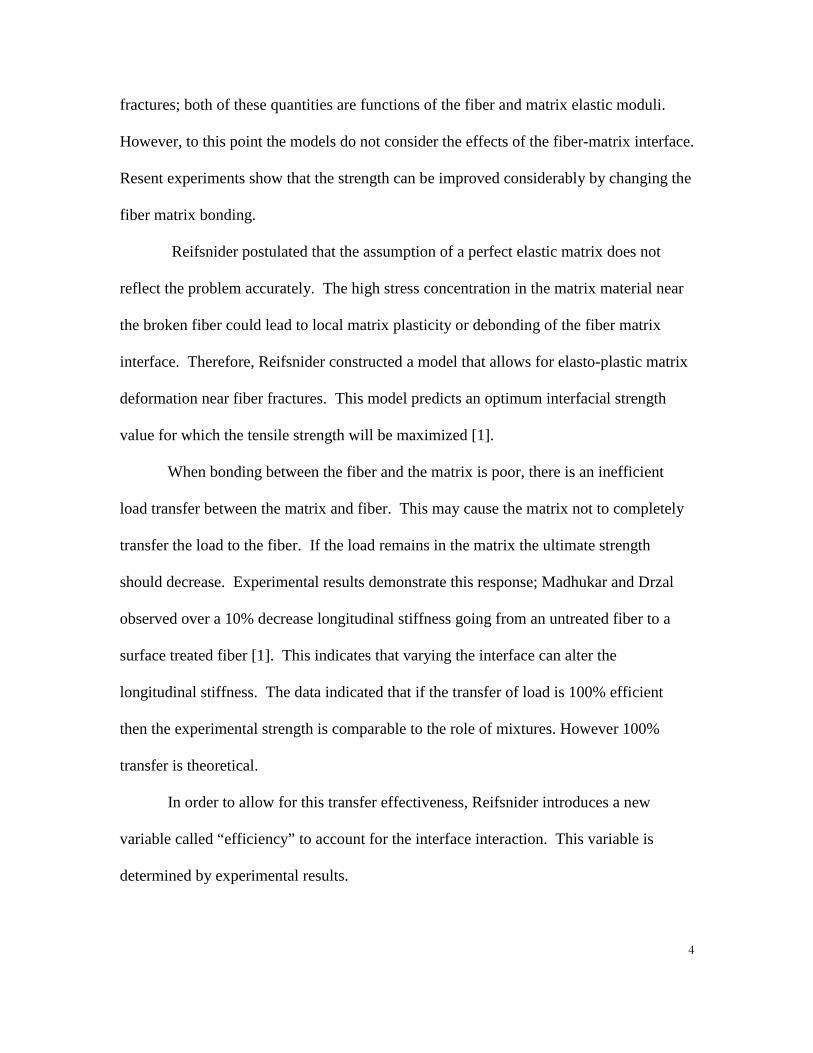
fractures; both of these quantities are functions of the fiber and matrix elastic moduli.

However, to this point the models do not consider the effects of the fiber-matrix interface.

Resent experiments show that the strength can be improved considerably by changing the

fiber matrix bonding.

Reifsnider postulated that the assumption of a perfect elastic matrix does not

reflect the problem accurately. The high stress concentration in the matrix material near

the broken fiber could lead to local matrix plasticity or debonding of the fiber matrix

interface. Therefore, Reifsnider constructed a model that allows for elasto-plastic matrix

deformation near fiber fractures. This model predicts an optimum interfacial strength

value for which the tensile strength will be maximized [1].

When bonding between the fiber and the matrix is poor, there is an inefficient

load transfer between the matrix and fiber. This may cause the matrix not to completely

transfer the load to the fiber. If the load remains in the matrix the ultimate strength

should decrease. Experimental results demonstrate this response; Madhukar and Drzal

observed over a 10% decrease longitudinal stiffness going from an untreated fiber to a

surface treated fiber [1]. This indicates that varying the interface can alter the

longitudinal stiffness. The data indicated that if the transfer of load is 100% efficient

then the experimental strength is comparable to the role of mixtures. However 100%

transfer is theoretical.

In order to allow for this transfer effectiveness, Reifsnider introduces a new

variable called “efficiency” to account for the interface interaction. This variable is

determined by experimental results.

�

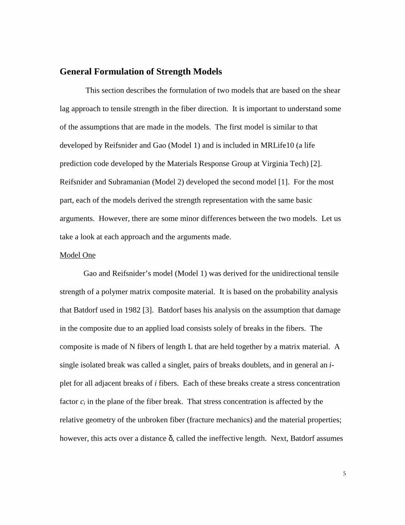
General Formulation of Strength Models

This section describes the formulation of two models that are based on the shear

lag approach to tensile strength in the fiber direction. It is important to understand some

of the assumptions that are made in the models. The first model is similar to that

developed by Reifsnider and Gao (Model 1) and is included in MRLife10 (a life

prediction code developed by the Materials Response Group at Virginia Tech) [2].

Reifsnider and Subramanian (Model 2) developed the second model [1]. For the most

part, each of the models derived the strength representation with the same basic

arguments. However, there are some minor differences between the two models. Let us

take a look at each approach and the arguments made.

Model One

Gao and Reifsnider’s model (Model 1) was derived for the unidirectional tensile

strength of a polymer matrix composite material. It is based on the probability analysis

that Batdorf used in 1982 [3]. Batdorf bases his analysis on the assumption that damage

in the composite due to an applied load consists solely of breaks in the fibers. The

composite is made of N fibers of length L that are held together by a matrix material. A

single isolated break was called a singlet, pairs of breaks doublets, and in general an i-

plet for all adjacent breaks of i fibers. Each of these breaks create a stress concentration

factor ci in the plane of the fiber break. That stress concentration is affected by the

relative geometry of the unbroken fiber (fracture mechanics) and the material properties;

however, this acts over a distance δ, called the ineffective length. Next, Batdorf assumes

�

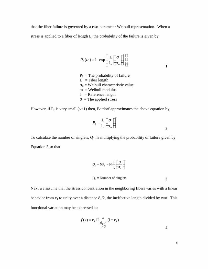
that the fiber failure is governed by a two-parameter Weibull representation. When a

stress is applied to a fiber of length L, the probability of the failure is given by

=

m

ofP

σσσ

ol

L -exp - 1 ) (

1

Pf = The probability of failureL = Fiber lengthσo = Weibull characteristic valuem = Weibull moduluslo = Reference lengthσ = The applied stress

However, if Pf is very small (<<1) then, Batdorf approximates the above equation by

m

ofP

=

σσ

ol

L

2

To calculate the number of singlets, Q1, is multiplying the probability of failure given by

Equation 3 so that

singlets ofNumber

l

lN NP

1

of1

=

==

Q

Q

m

oσσ

3

Next we assume that the stress concentration in the neighboring fibers varies with a linear

behavior from c1 to unity over a distance δ1/2, the ineffective length divided by two. This

functional variation may be expressed as:

)c 1(

2

z c )( 1

11 −+= δzf

4

�

Reifsnider expressed the reliability of the fiber having a stress variation of this type given

by:

=

m

ao

Rσσ

-exp

5

where the variable σao is defined by intergration over the length of the fiber.

[ ]mL

o

mao zf

1

o dz )(

−

= ∫σσ

6

Now these relations can be combined in equation 4 to show that the probability of failure

in the over-stressed region may be approximated by:

m

cP

≈

o1

o

11

l

σσλ

7

where the variable λ1 contains the distance (ineffective length) and stress concentration.

)1)(1(

1c

11

1m1

11 +−−

=+

mccmδλ

8

Next the development considers the probability that a singlet becomes a doublet. If there

are n1 nearest neighbors, then this probability is given by:

m

cP

=→

o1

o

1121

l n

σσλ

9

Using equation 3, an estimate of the number of doublets is derived as:

�

m

cnQ

=

oo

1112

l Q

σσλ

10

Repeating this process leads to a general model to estimate the number of i-plets:

m

iii cnQ

=+

oo

ii1

l Q

σσλ

11

or as

o

jj

i

j

mj

im

oi l

ncQλ

σσ ∏

−

=

=

1

1ol

LN

12

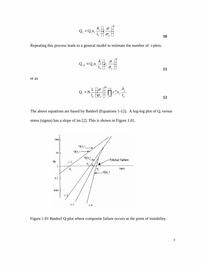
The above equations are based by Batdorf (Equations 1-12). A log-log plot of Qi versus

stress (sigma) has a slope of im [2]. This is shown in Figure 1.01.

Figure 1.01 Batdorf Q-plot where composite failure occurs at the point of instability.

�

The failure stress is given by the lowest stress at which any unstable i-plet is formed.

Therefore, the stress at which the envelope intersects the horizontal line Qi = 1 or ln Qi =

0, is the failure stress. The only thing left to determine are the stress concentrations and

the ineffective lengths for each number of adjacent fiber fractures. Gao and Reifsnider

used a shear-lag model to determine these two values [3].

Gao and Reifsnider start by making an assumption that there is a central core of

broken fibers as shown in Figure 1.02 [3]. The broken fiber are surrounded by unbroken

fibers that are being strained. The core of broken fibers is assumed to be a homogeneous

material whose Young’s modulus is obtained by the rule of mixtures. The assumed

circular cross sectional areas of the equivalent broken core is equal to the total area of the

ith concentric cylinder of radius rf + d.

regionmatrix of width theof half d

fiber theof radius the

)(ri r 2f

2o

=

=

+=+=

f

mf

r

iAiAdππ

13

The variables correspond to the concentric cylinder model given in Figure 1.02 [4].

��

2d 2d 2d 2d

x

U 1 U 2U 0

Broken Composite

Matrix

Fiber

Bulk Composite

Zone of matrix yielding

Crack

r0

r - d0

r + d0

r + df

d

Concentric Cylinder

a

Figure 1.02 Fiber fracture of unidirectional composites used by Gao and Reifsnider.

The fiber area and matrix area are given by:

�

II U$ π= 14

( ) 22f d r fm rA ππ −+=

15

The number of neighboring unbroken fibers, ni, is dependent upon the number of

broken fibers, i. The assumption is made that only the fibers carry the axial stress and the

��

matrix only supports shear (the classical shear lag assumptions). The distance

measurement "a" gives the half-length of the region of matrix and/or interfacial yielding.

The equilibrium equations for this region of the matrix and interfacial yielding are given

as:

ax

rUUd

Grdr

dx

UdEA

rdx

UddrE

oom

foff

ooo

o

≤≤

=+−+++

=−−

0

0 2)(2

)22(2n

0 2)(

1221

2

i

2

22

ητππ

ητππ

16

Uo = Displacements of the broken coreU1 = Displacements of neighboring unbroken fiberU2 = Displacements of average compositeEf = Young’s modulus of the fiberGm = Shear modulus of the matrixAf = Area of the fiberτo = Yielding stress of the matrix and interfaceη = a shear parameter, efficiency factor

The efficiency factor parameter defines the efficiency nature of the shear transfer

in the inelastic region. This parameter has the value between one and zero with zero

being no shear stress transfer between broken fibers and their neighbors in the region.

This is a representation of a complete fiber-matrix debonding of matrix cracking in the

region.

Using the rule of mixtures, the Young’s modulus of the broken core, E, is

determined to be:

��

[ ]2

o

22mff

)(r

))((iAEiA

d

EdrrE moo

−−−−+

=π

π

17

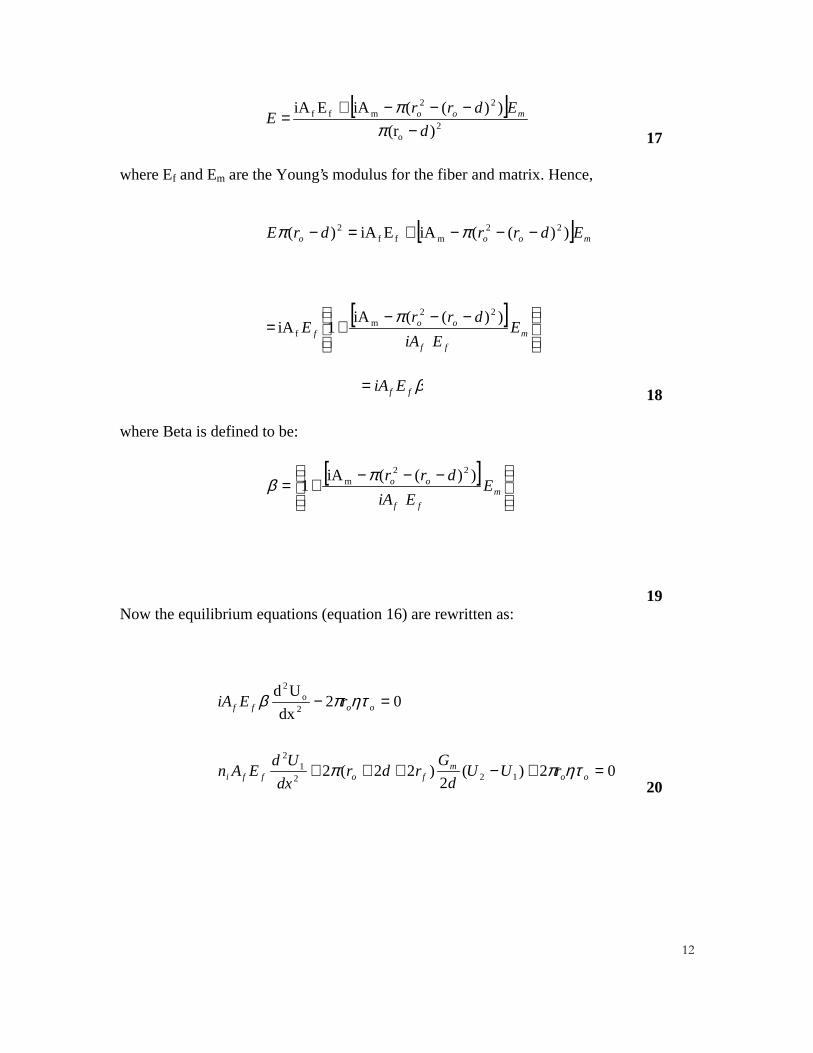
where Ef and Em are the Young’s modulus for the fiber and matrix. Hence,

[ ] mooo EdrrdrE ))((iAEiA)( 22mff

2 −−−+=− ππ

[ ]

−−−

+= m

ff

oof E

EiA

drrE

))((iA1iA

22m

f

π

βff EiA=18

where Beta is defined to be:

[ ]

−−−

+= m

ff

oo EEiA

drr ))((iA1

22m πβ

19Now the equilibrium equations (equation 16) are rewritten as:

02)(2

)22(2

02dx

Ud

1221

2

2o

2

=+−+++

=−

oom

foffi

ooff

rUUd

Grdr

dx

UdEAn

rEiA

ητππ

ητπβ

20

��

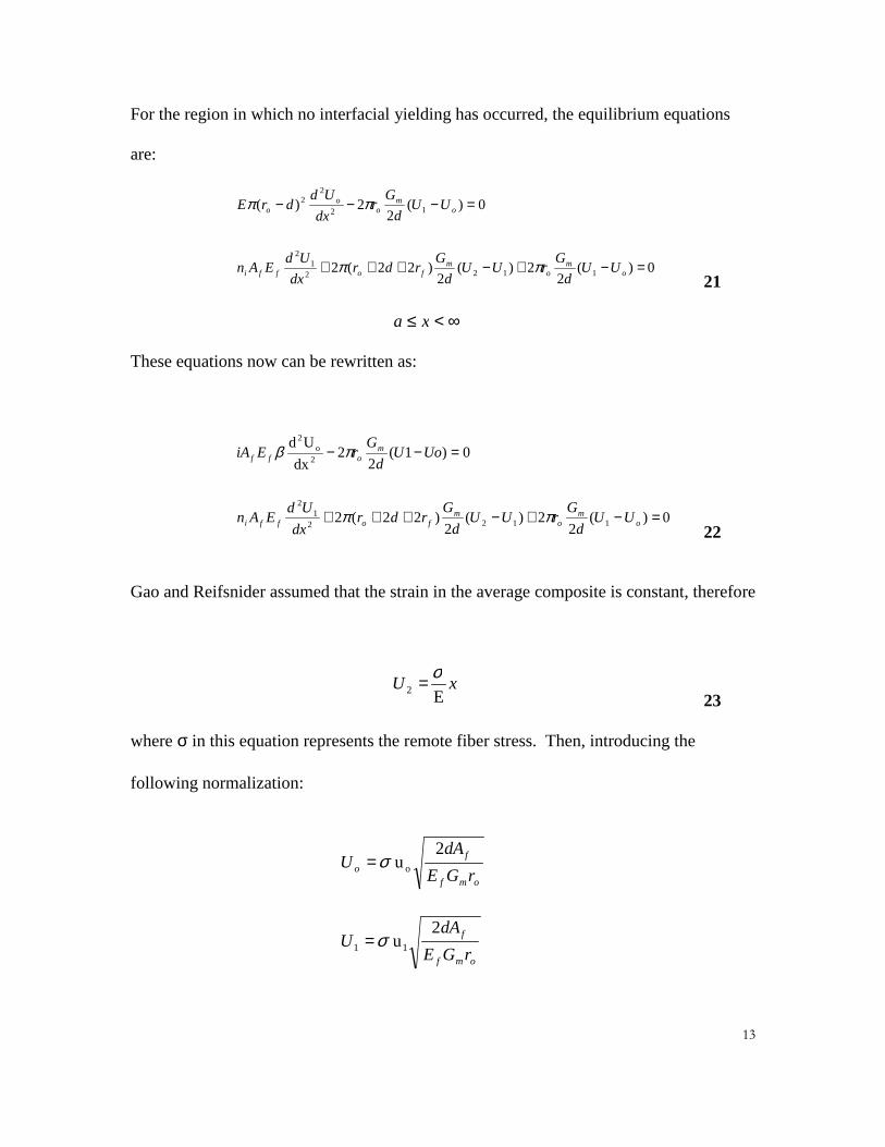
For the region in which no interfacial yielding has occurred, the equilibrium equations

are:

0 )(2

2)(2

)22(2

0)(2

2)(

11221

2

12

22

=−+−+++

=−−−

om

om

foffi

om

oo

o

UUd

GrUU

d

Grdr

dx

UdEAn

UUd

Gr

dx

UddrE

ππ

ππ

21

∞<≤ xa

These equations now can be rewritten as:

0 )(2

2)(2

)22(2

0)1(2

2dx

Ud

11221

2

2o

2

=−+−+++

=−−

om

om

foffi

moff

UUd

GrUU

d

Grdr

dx

UdEAn

UoUd

GrEiA

ππ

πβ

22

Gao and Reifsnider assumed that the strain in the average composite is constant, therefore

xUE

2

σ=23

where σ in this equation represents the remote fiber stress. Then, introducing the

following normalization:

omf

fo rGE

dAU

2u oσ=

omf

f

rGE

dAU

2u 11 σ=

��

om

ff

rG

dE2A ζ=x

of

mf

r2dE

GA σττ oo =

om

ff

rG

dE2Aα=a24

We can rewrite the equilibrium equations as

0 i

2 -

2

2

=oo

d

ud τηβπ

ξ

0) t( tu 121

2

=++− ξτηφφζ

od

ud

∞<≤ ζ0 25

with

0)(2

12

2

=−+ oo uu

id

ud

βπ

ζ

ζφφφζ

tud

udo - t)u(1- 12

12

=++26

∞<≤ ζα

where

o

fo

r

2r2dr

++=t

27

��

in

πφ 2=28

In order to solve the second order differential equations, two boundary conditions must

be applied. They are as follows:

1)()(

0)0()0(

1

1

=∞

=∞

==

ζζ

ζ

d

du

d

du

ud

du

o

o

29

The solution to the second order differential equation (equations 26) is as follows:

12 A

iu

o

o += ζβτπη

)exp()t

()exp( 221 φζτζφζζτηtAtA

tu

oo −+−++=30

The constants A1 and A2 will be determined from continuity conditions.

The solution to equations 27 can be written as follows:

)exp()1()exp()1( 22

211

1 ζλφλζλ

φλζ −−++−−++= tBtBuo

)exp()exp( 22111 ζλζλζ −+−+= BBu 31

where B1 and B2 are constants with

��

{ }i

ii nititntin

βπβββλ 22

i2

1 )1()()1(n2i )1( ++−+++=

{ }i

ii nititntin

βπβββλ 22

i2

2 )1()()1(n2i )1( ++−−++=32

The stress concentration on the unbroken fibers is expressed as;

ζζζ

d

duCi

)()( 1=

33and the dimensionless shear stress is expressed as:

1)( uuo −=ζτ 34

The finial equation used to predict the strength of the composite is shown below.

Fiber of Stiffness E

Matrix of Stiffness E

Stress Critical ˆ

Fraction VolumeFiber V

E

ˆ )EV-(1 ˆ V

f

m

c

f

fmfc f

====

•+•=

σ

σσ ctX

35

Case and Reifsnider have developed a computer code based on the above

arguments for strength with a polymer matrix composite. This code (MRLife) is written

in "C++" and the results from this code will be used to compare with the experimental

results [2].

��

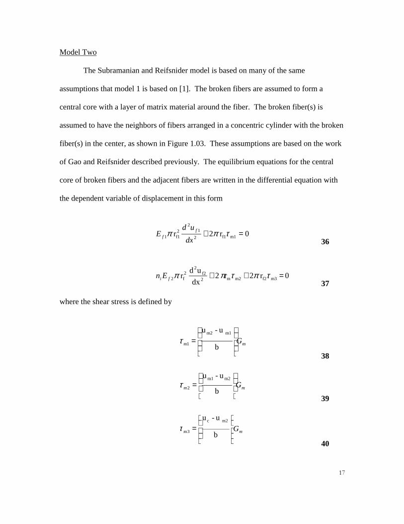
Model Two

The Subramanian and Reifsnider model is based on many of the same

assumptions that model 1 is based on [1]. The broken fibers are assumed to form a

central core with a layer of matrix material around the fiber. The broken fiber(s) is

assumed to have the neighbors of fibers arranged in a concentric cylinder with the broken

fiber(s) in the center, as shown in Figure 1.03. These assumptions are based on the work

of Gao and Reifsnider described previously. The equilibrium equations for the central

core of broken fibers and the adjacent fibers are written in the differential equation with

the dependent variable of displacement in this form

0r 2 r m1f12

12

2f11 =+ τππ

dx

udE f

f36

0 r 2 r 2 dx

ud r m3f2m2m2

f22

2f2 =++ τπτππfi En

37

where the shear stress is defined by

mm G

=

b

u - u

m1m2

1τ

38

mm G

=

b

u - u

m2m1

2τ

39

mG

=

b

u-u m2c

3mτ

40

��

Figure 1.03 Schematic of concentric cylinder model with a core of broken fibers with theneighboring fibers.

These equations are based on the assumption that the displacement varies linearly

in the radial direction in the matrix material. The fibers are also assumed to carry all the

axial load with the matrix around the fibers acting only to transfer the load between the

fibers through a shear transfer mechanism. Assuming that the displacement in the fiber

and matrix at the fiber-matrix interface is discontinuous, and that the displacement in the

average composite is uniform, the following expressions can be written

x

a

E

xuc

σ=

41

m11 u η=fu42

��

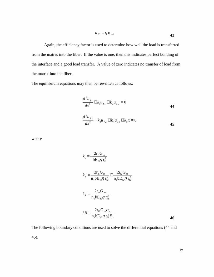
m22 u η=fu43

Again, the efficiency factor is used to determine how well the load is transferred

from the matrix into the fiber. If the value is one, then this indicates perfect bonding of

the interface and a good load transfer. A value of zero indicates no transfer of load from

the matrix into the fiber.

The equilibrium equations may then be rewritten as follows:

022112

12

=++ fff ukuk

dx

ud

44

0514232

22

=++− xkukukdx

udff

f

45

where

x

a

Ek

k

k

k

2f2f2i

mf2

2f2f2i

mm4

2f2f2i

mf22f2f2i

mm3

2f1f1

mf11

r bEn

G2r5

r bEn

G2r

r bEn

G2r

r bEn

G2r

r bE

G2r-

ησ

η

ηη

η

=

=

+=

=

46

The following boundary conditions are used to solve the differential equations (44 and

45).

��

���

�

��

�

�

=

=

=

=

[I

[

I

X

G[

GX

47

Solving the differential equations yields:

0)]()([ 52231423124 =−+−−+ xkkukkkkkkDD f 48

The homogenous solution to the differential equation requires that

xxxxf

xxxxf

eDeDxDeDeDu

eCeCxCeCeCu

βαβα

βαβα

543212

543211

++++=

++++=

−−

−−

49

where2/1

422

3113

2

4)()(,

++±−=

kkkkkkβα

50

The following constants must be zero in order for the fiber strains to be finite at

regions far away from the fiber fracture; C4 , C5, D4, and D5. Next the assumed

displacement functions are substituted into the equilibrium equations and the remaining

constants are determined.

��

12

12

2

12

2

31

21

22

2

11

22

1

33

4231

523

kk-

DD

k

k

k

k

CD

Dk

kC

Dk

kC

CD

kkkkC

−=

+

−+

=

+

−=

+

−=

−=

+=

αα

ββ

β

α

51

Now the solution to the displacements is obtained

xDeDeDu

xCeCeCu

xxf

xxf

3212

3211

++=

++=

−−

−−

βα

βα

52

The strains and stresses in the central core and the adjacent fibers are derived using the

strain-displacement and constitutive relationships of mechanics of materials.

f2f2f22

f2

f11f11

f1

E ;

;

εσε

εσε

==

==

dx

du

Edx

du

f

ff

53

��

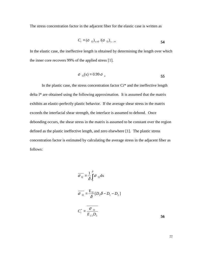
The stress concentration factor in the adjacent fiber for the elastic case is written as

∞→== xf20xf2 ) /() ( σσiC 54

In the elastic case, the ineffective length is obtained by determining the length over which

the inner core recovers 99% of the applied stress [1].

af1 0.99(x) σσ = 55

In the plastic case, the stress concentration factor Ci* and the ineffective length

delta I* are obtained using the following approximation. It is assumed that the matrix

exhibits an elastic-perfectly plastic behavior. If the average shear stress in the matrix

exceeds the interfacial shear strength, the interface is assumed to debond. Once

debonding occurs, the shear stress in the matrix is assumed to be constant over the region

defined as the plastic ineffective length, and zero elsewhere [1]. The plastic stress

concentration factor is estimated by calculating the average stress in the adjacent fiber as

follows:

32

f2*

213f2

f2

0

f2f2

][E

dx 1

DEC

DDD

fi

σ

δδ

σ

σδ

σδ

=

−−=

= ∫

56

��

For the elastic-perfectly plastic case, the stress concentration factor will be equal to one.

The force balance argument is used to estimate the plastic ineffective length as follows:

i

1f1*

2

τησ

δ fi

r=

57

where the average stress in the inner core is given by

)(

2131

f1

0

f11

f1

CCCE

dxE

f

f

−−=

= ∫

δδ

σ

εδ

σδ

58

When writing the force balance equation, it was assumed that due to interfacial

debonding the shear stress in the matrix is not equal to the interfacial shear strength, but

is multiplied by the efficiency factor. Once debonding has occurred the transfer of stress

is done with a mechanism of friction. After debonding it is assumed that the stress

transfer will not be perfect. The shear stress is multiplied by the efficiency factor to

reflect this behavior [1].

Now that the stress concentration factor and the ineffective lengths have been

derived for both cases of plastic and elastic local behavior for different fiber breakages,

the tensile strength is predicted following Batdorf’s analysis. As previously discussed,

Batdorf showed that the stress level at which the first fiber fracture occurs is expressed

as:

��

fiber for theparameter location strength Weibull

fiber for thefactor shapestrength Weibullm

specimen theoflength normalizedL

specimen in the fibers ofnumber

NL

1

o

o

/1

1

====

=

σ

σσ

totalN

m

59

The stress level at which the next fiber fractures occur is given by

2,3,...i n

1o

/1

1-i1-i

=

= σ

λπσ

m

i NL 60

and

( )

+−

−=

+

)1(1

12

1

mC

C

i

mi

ii δλ61

The average shear stress in the matrix region is estimated as follows

( )

−+−=

−

= ∫

βαηδτ

δτ

δ

)(

1

2211

0

12

CDCD

b

G

dxGb

uu

mm

mmm

m

62

It is assumed that interfacial debonding occurs when the average shear stress in

the matrix exceeds the interfacial shear strength. At each load level, calculations are

made to see if the interfacial failure occurs. Once the interfacial failure occurs then the

��

plastic stress factor and ineffective lengths are used to predict fiber fractures. However,

if there is no interfacial failure until instability occurs, then the final failure is classified

as elastic failure. If the debonding occurs before the final failure, the failure is termed

plastic.

Model 2 can be used to predict failure of an unidirectional laminate for tensile

strength. A computer code that makes the looped calculations of this model is written in

Pascal.

Quantitative Differences between the Models

As previously mentioned, both of the models are based on the classical shear lag

arguments. However there are some differences between the two models. Model 1

assumes that the displacement in the fiber and matrix outside the yielding region to be

continuos at the fiber-matrix interface. Model 2 admits displacement discontinuities

between the fiber and matrix outside the yielding zone. Model 1 uses the maximum shear

stress value in the matrix to determine if yielding occurs. Model 2 uses the average shear

stress value in the matrix to determine if yielding occurs. Other differences maybe

between the assumed geometry of the fiber matrix regions.

Temperature Effects on the Strength

Many researchers have tried to understand the effects of elevated temperatures on

composite materials. Many questions still remain about the effect. For example, how

does the temperature affect the material system with respect to creep recovery and visco-

��

elastic-plastic behavior. More important is how we express these behaviors in terms of

known constitutive equations [5].

The approach to these questions has been to identify the failure mode(s) that

control fracture, and to set up a boundary value problem that represents the micro-details

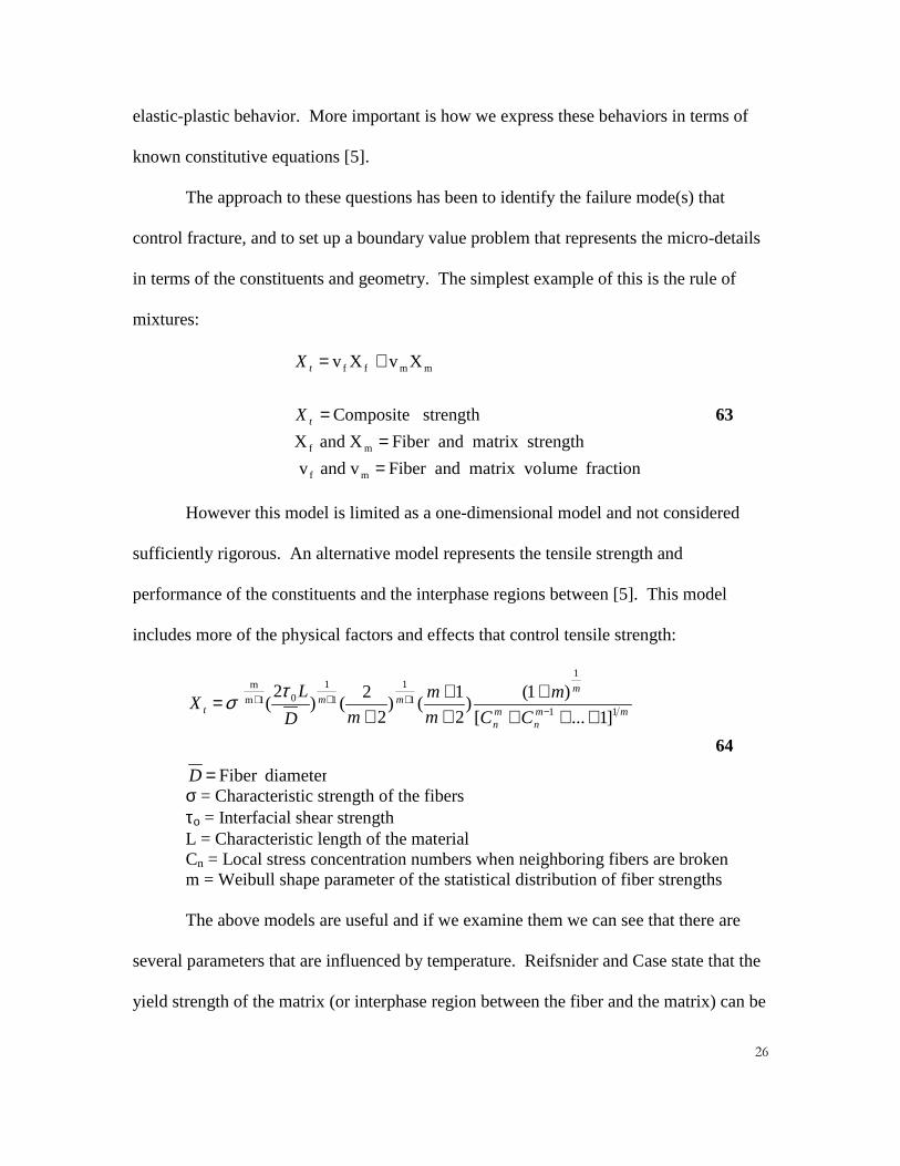
in terms of the constituents and geometry. The simplest example of this is the rule of

mixtures:

fraction lumematrix vo andFiber vand v

strengthmatrix andFiber X and X

strength Composite

X v X v

mf

mf

mmff

==

=

+=

t

t

X

X

63

However this model is limited as a one-dimensional model and not considered

sufficiently rigorous. An alternative model represents the tensile strength and

performance of the constituents and the interphase regions between [5]. This model

includes more of the physical factors and effects that control tensile strength:

diameterFiber

]1...[

)1()

2

1()

2

2()

2(

11

1

1

1

1

101m

m

=

++++

++

+= −

+++

D

CC

m

m

m

mD

LX

mmn

mn

mmm

t

τσ

64

σ = Characteristic strength of the fibersτο = Interfacial shear strengthL = Characteristic length of the materialCn = Local stress concentration numbers when neighboring fibers are brokenm = Weibull shape parameter of the statistical distribution of fiber strengths

The above models are useful and if we examine them we can see that there are

several parameters that are influenced by temperature. Reifsnider and Case state that the

yield strength of the matrix (or interphase region between the fiber and the matrix) can be

��

expected to decrease with increasing temperature [5]. Also, the stiffness of the

components will, in general, be a function of temperature. For a polymer matrix material,

for example, the shear stiffness will often be strongly temperature dependent [5].

Furthermore, temperature also effects the ineffective length. As discussed, the

ineffective length is created in the region of a fiber fracture. When a fiber breaks, the

stress is transferred back into a neighboring fiber by the surrounding matrix in a manner

that is controlled by the stiffness of the surrounding material. As the surrounding

material becomes less stiff, the ineffective length becomes larger. If the ineffective

length is large, then the fiber fracture regions will interact more easily and may connect

together to cause complete failure [5]. However, if the matrix material and surrounding

composite is very stiff, then the stress is transferred back into the fiber over a small

distance and the ineffective length is small. In this case, the stress concentration in the

material next to a fiber break is very high. This greatly increases the chance of one fiber

fracture causing an unstable sequence of neighboring fiber fractures resulting in complete

failure. A shear lag equation for the ineffective length is as follows:

transferstress for thefactor Efficiency

fibers theof Stiffness

stiffnessMatrix

fiber thef ofraction Volume

length eIneffectiv

)1

1ln()])(

1(

2

1[

2

1 2

1

5.0

5.0

=

==

==

−−

=

φ

νδ

φδ

f

m

f

m

f

f

f

E

G

G

E

v

v

65

Case and Reifsnider pointed out that elevated temperature reduces the stiffness of

the matrix and with this reduction the ineffective length will increase. Under this

��

assumption, the strength equation should express what happens to the composite strength.

If the increase in temperature causes the ineffective length to increase, then the composite

strength may respond with an increase or decrease. The basic assumption is that as the

temperature is elevated, the polymer matrix stiffness will reduce and with this

phenomena the ineffective length will increase. The effect of the ineffective length on

the strength is demonstrated in the following figure (Figure 1.04) [5].

Tensile Strength as a Function of Ineffective Length

0

0.5

1

1.5

2

2.5

3

3.5

0 1 2 3 4 5 6

Normalized Ineffective Length

Co

mp

osi

te S

tren

gth

m=2

m=6

Figure 1.04 Tensile strength as a function of local ineffective length.

This figure (Figure 1.04) is generated for different ineffective length values with

two different Weibull shape factors (m). Clearly, this figure indicates that there is a

location were the strength is maximum. To the left of the maximum, strength is reduced

��

by a stress concentration due to the small ineffective length that causes a brittle fracture.

To the right of the maximum, the strength is reduced by the greater ineffective length

because of the coupling of fiber fracture zones. Therefore, as the elevated temperatures

cause the ineffective length to change, the strength may increase or decrease based on the

position of the value for the ineffective length [5].

Using some data we can demonstrate the strength increases and decreases with the

change of elevated temperature (Figure 1.05). The IM7/K3B system was tested in our

laboratory and the Graphite/Epoxy system was tested by Haskins [6].

Tensile Strength of Graphite Epoxy system and IM7/K3B system

0

50

100

150

200

250

300

350

400

450

-100 -50 0 50 100 150 200 250 300 350 400

Temperature (F)

Str

eng

th (

ksi)

IM7/K3B

Graphite Epoxy

Figure 1.05 Unidirectional tensile strength as a function of temperature for two polymercarbon fiber composites.

��

This figure indicates that, depending on the matrix material, we can be to the left

of the ineffective length temperature maximum or to the right of this maximum.

Observing the Graphite/Epoxy system in Figure 1.05, the indication is that this system is

to the left of the maximum in Figure 1.04. However the IM7/K3B system indicates that

the strength is to the right of the maximum in Figure 1.04.

Interfacial Shear Strength at Elevated Temperatures

Both of the above models use the interfacial shear strength as a parameter in the

formulation of the strength. Many researches have spent time investigating the fiber-

matrix shear strength. The matrix polymer adhering to the fiber surface produces this

strength. An investigation was performed on the interfacial adhesion on carbon fiber at

elevated temperatures by H. Zhuang and J.P. Wightman [7]. This evaluation is also

known as single fiber fracture testing.

The testing was conducted on various carbon fibers in a single "dog bone"

specimens of epoxy matrix. Preparation of the single fiber composite was as follows: a

silicone rubber mold with a dog-bone-shaped cavity was used to give the composite its

shape during cure of the epoxy. A single fiber was fixed on both ends with the middle

suspended in the mold. Epoxy resin was poured in the mold with the fiber embedded in

the epoxy. The cure schedule was 75 degrees C for 2 hours and then 125 degrees C for

another 2 hours. Then the specimens were allowed to cool overnight and removed from

the mold [7].

The fragmentation test was preformed as follows: the single fiber specimens were

mounted in a hand operated loading fixture one at a time. The specimens were observed

with a transmitting-light microscope. The specimens were then pulled in tension at a

��

speed of 1 mm/min and the fiber fractures were observed during this process. The

tension on the specimen was stopped after no further breaks were observed with

increasing load. The fragment lengths then were measured with the aid of the

microscope and recorded.

The same procedure was used for the elevated temperature fragmentation tests.

However, the fixture was placed in a hot oil bath with the oil at the desired temperature.

The specimens were given 10 minutes in the oil bath to allow for the heat transfer [7].

The equation used to determine the interfacial shear strength was as follows.

length critical l

diameterfiber d

length critical at thestrength fiber

strengthshear linterfacia

2

c

f

==

==

=

στ

στ

c

f

l

d

66

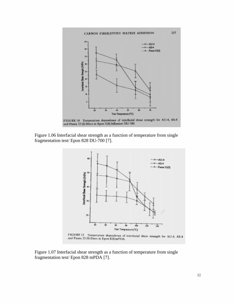
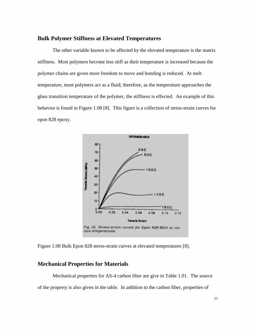
Figure 1.06 and Figure 1.07 show the response of the interfacial shear strength as

a function of temperature. Three different fibers were used to examine the adhesion

process on the fibers for a single matrix material. The carbon fibers were AS-4, AU-4

and Panex 33 (S) and the epoxy was Epon 828. Two different curing agents were used

on the epoxy. Figure 1.06 shows the response with the Jeffamine DU-700 curing agent

and Figure 1.07 shows the response with mPDA curing agent [7].

The results show that the interfacial shear strength decreases as a function of

temperature. The trend from one carbon fiber system to another system can vary, and the

curing agent can also effect the strength value.

��

Figure 1.06 Interfacial shear strength as a function of temperature from singlefragmentation test/ Epon 828 DU-700 [7].

Figure 1.07 Interfacial shear strength as a function of temperature from singlefragmentation test/ Epon 828 mPDA [7].

��

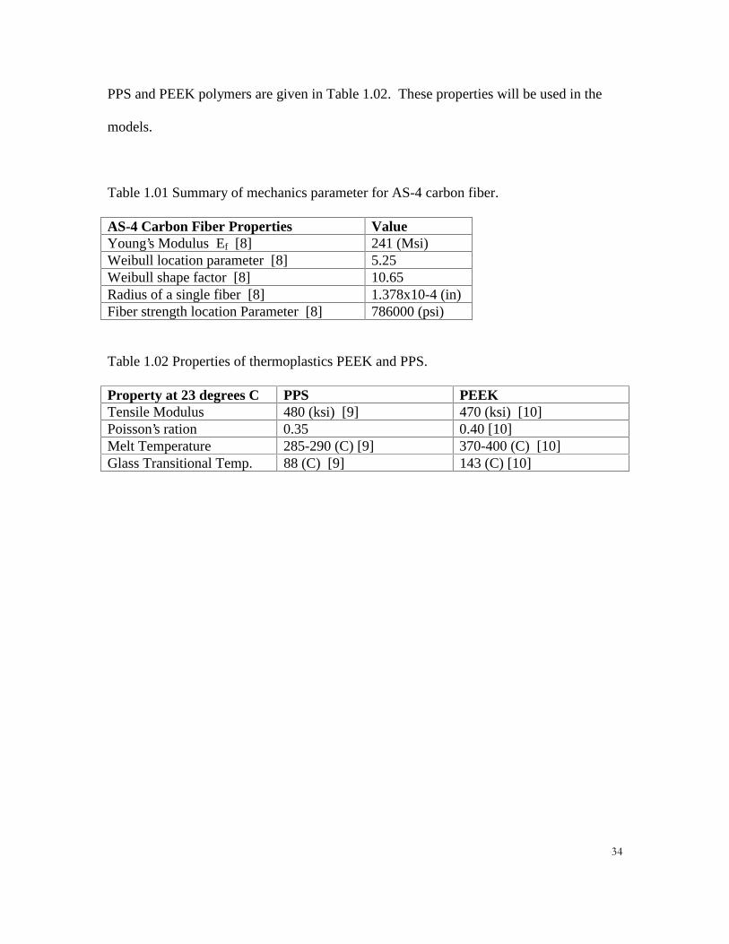
Bulk Polymer Stiffness at Elevated Temperatures

The other variable known to be affected by the elevated temperature is the matrix

stiffness. Most polymers become less stiff as their temperature is increased because the

polymer chains are given more freedom to move and bonding is reduced. At melt

temperature, most polymers act as a fluid; therefore, as the temperature approaches the

glass transition temperature of the polymer, the stiffness is effected. An example of this

behavior is found in Figure 1.08 [8]. This figure is a collection of stress-strain curves for

epon 828 epoxy.

Figure 1.08 Bulk Epon 828 stress-strain curves at elevated temperatures [8].

Mechanical Properties for Materials

Mechanical properties for AS-4 carbon fiber are give in Table 1.01. The source

of the property is also given in the table. In addition to the carbon fiber, properties of

��

PPS and PEEK polymers are given in Table 1.02. These properties will be used in the

models.

Table 1.01 Summary of mechanics parameter for AS-4 carbon fiber.

AS-4 Carbon Fiber Properties ValueYoung’s Modulus Ef [8] 241 (Msi)Weibull location parameter [8] 5.25Weibull shape factor [8] 10.65Radius of a single fiber [8] 1.378x10-4 (in)Fiber strength location Parameter [8] 786000 (psi)

Table 1.02 Properties of thermoplastics PEEK and PPS.

Property at 23 degrees C PPS PEEKTensile Modulus 480 (ksi) [9] 470 (ksi) [10]Poisson’s ration 0.35 0.40 [10]Melt Temperature 285-290 (C) [9] 370-400 (C) [10]Glass Transitional Temp. 88 (C) [9] 143 (C) [10]

��

II. Experimental Procedures

General Equipment

XPS

X-ray Photoelectron Spectroscopy (XPS) was used to determine the surface

chemistry of material that was supplied in test form. XPS involves the bombardment of

the specimen surface with mono-energetic X-rays in a high vacuum. As the photons

travel through the material some are absorbed and their energy is transferred to electrons

which can be ejected from the specimen. The spectrum, the electron intensity versus the

binding energy of the electron to the atom, is obtained by pulse-counting techniques

[11].

This test was used to supplement information about the composites’ chemistry.

The PPS system was the only system that was delivered ready to test and the company,

Polymer Composite International (P.C.I.) did not disclose any processing information.

Therefore it was necessary to use this test to obtain some information about the

composite.

��

Fiber Volume Fraction Analysis

The fiber volume fraction for each material was determined by a buoyancy test.

Several samples were taken from each material type. The dry weight of each sample was

measured on an electronic balance. Then the samples were weighed submerged in

isopropanol. Knowing the density of the resin, fiber, and isopropanol the fiber volume

can be calculated with the following equations:

lIsopropano ofDensity

lIsopropanoin Composite ofWeight W

(g)air in Composite ofWeight

(g/cc) Composite ofDensity

*

iso

iso

iso

===

=

−=

ρ

ρ

ρρ

air

c

isoair

airc

W

WW

W

(g/cc)Resin ofDensity

(g/cc)Fiber ofDensity

Compositein Fiber offraction Volume

resin

fiber

sin

sin

==

=

−−

=

ρρ

ρρρρ

f

refiber

recf

V

V

C-Scans

A Scanning Acoustic Microscope C-Scan was preformed on the PEEK panels to

detect flaws. This instrument uses sound waves to penetrate the panel and uses the

returning sound wave to interrogate the material’s make up. The panel was placed in a

bath of water for a short period of time (10 minutes) while the C-Scan was preformed.

��

If the time of flight of the sound wave is different in some places of the material,

the image will display this variation. This method is a nondestructive test that has limited

use. The instrument can help detect a flaw in the panels, such as, a fiber rich region or a

matrix rich region. If a flaw is detected then the defected section of the panel can be

discarded to avoid experimental discrepancies.

DMA

A Dynamic Mechanical Analysis (DMA) was used to determine the glass

transition temperature (Tg) for the composite systems. Many times the glass transition

temperature of the composite system is different than the bulk polymer’s glass transition

temperature. This measurement was used only to get an approximate glass transition

temperature and was not used to estimate any mechanical properties.

Quasi-static Tension Macro-Mechanical Test

The tension tests were conducted on a MTS hydraulic closed loop axial loading

machine. The grip pressure was determined by running a few specimens and increased if

slipping occurred. The final grip pressure was determined to be between 700 and 1000

pounds per square inch.

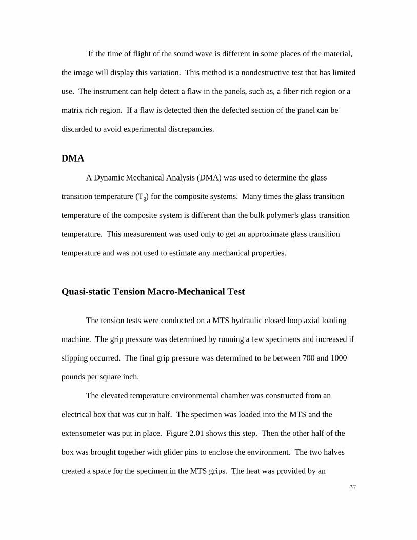
The elevated temperature environmental chamber was constructed from an

electrical box that was cut in half. The specimen was loaded into the MTS and the

extensometer was put in place. Figure 2.01 shows this step. Then the other half of the

box was brought together with glider pins to enclose the environment. The two halves

created a space for the specimen in the MTS grips. The heat was provided by an

��

industrial hot air blower and was controlled with an Omega Controller. The controller

cycled the current to the every 2 seconds. The heat environment was placed around the

specimen for a time period and was maintained until failure was achieved. A dummy

strain gage was also placed in this environment to provide thermal compensation.

Figure 2.01 MTS with heater box set up with a specimen.

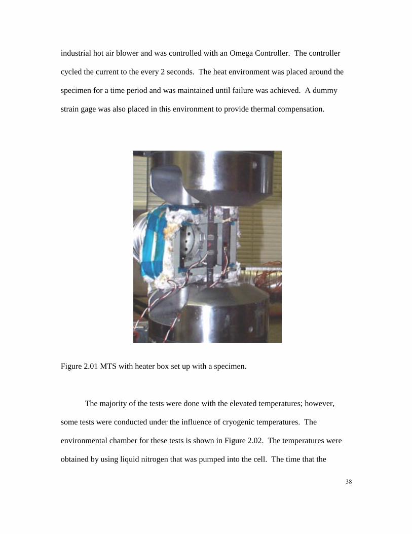
The majority of the tests were done with the elevated temperatures; however,

some tests were conducted under the influence of cryogenic temperatures. The

environmental chamber for these tests is shown in Figure 2.02. The temperatures were

obtained by using liquid nitrogen that was pumped into the cell. The time that the

��

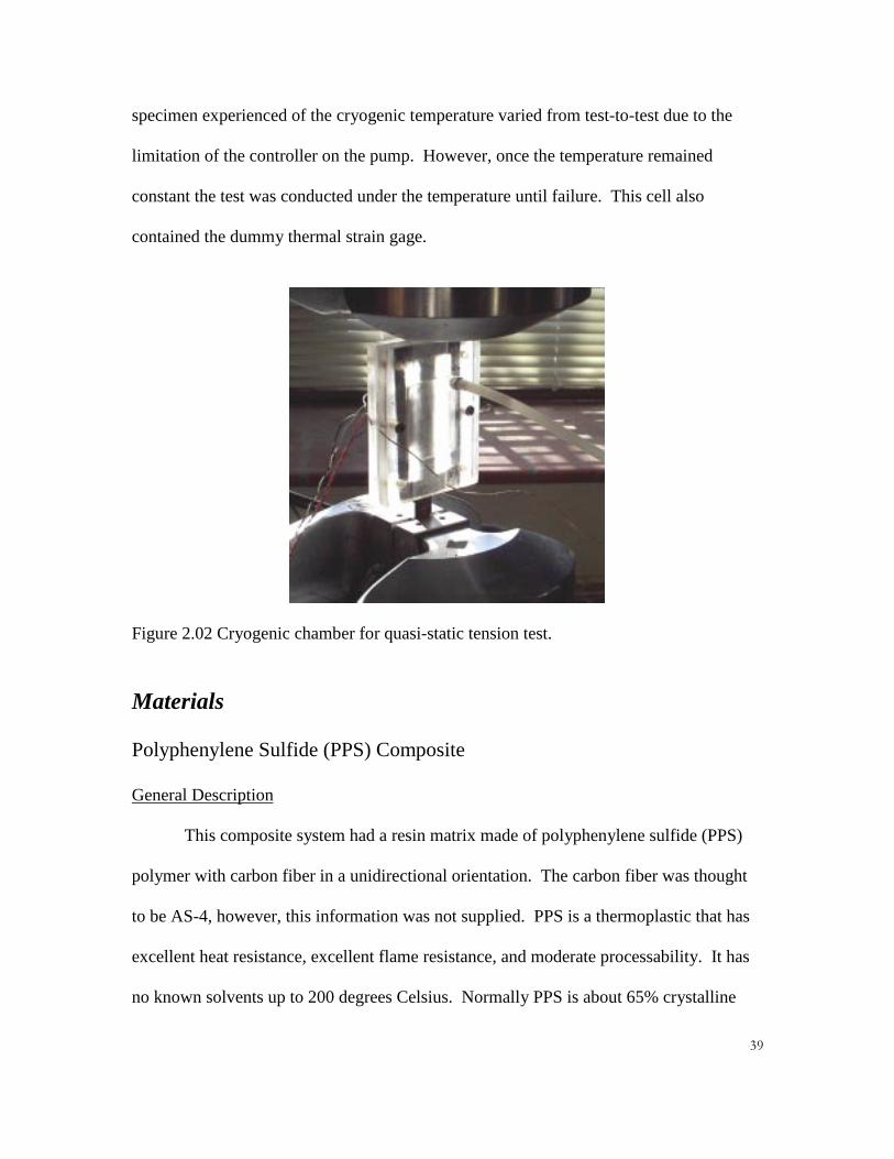
specimen experienced of the cryogenic temperature varied from test-to-test due to the

limitation of the controller on the pump. However, once the temperature remained

constant the test was conducted under the temperature until failure. This cell also

contained the dummy thermal strain gage.

Figure 2.02 Cryogenic chamber for quasi-static tension test.

Materials

Polyphenylene Sulfide (PPS) Composite

General Description

This composite system had a resin matrix made of polyphenylene sulfide (PPS)

polymer with carbon fiber in a unidirectional orientation. The carbon fiber was thought

to be AS-4, however, this information was not supplied. PPS is a thermoplastic that has

excellent heat resistance, excellent flame resistance, and moderate processability. It has

no known solvents up to 200 degrees Celsius. Normally PPS is about 65% crystalline

��

and has a glass transition temperature of 85 degrees Celsius. [10]. The low Tg value is

due to the flexible sulfide linkage between the aromatic rings [10].

Processing

Polymer Composite International (P.C.I.) manufactured the material on a spool

with an average thickness of 0.025 inches and a width of 0.48 inches. Limited

information was provided concerning the material’s chemistry or manufacturing process.

Specimen Preparation

The specimens were cut to 8 inches from the spool. Each specimen was grit

blasted using silicone on both ends one inch towards the center. One-inch fiberglass tabs

were then placed with an adhesive on both ends with the composite sandwiched between

them. The adhesive then was cured at 50 degrees Celsius for 2 hours. Figure 2.03 shows

the dimensions of a typical specimen. If strain measurements were conducted in the test,

extensometer tabs or strain gages were fixed in the middles on the surface. Strain gages

were supplied by Micro-Measurements, Inc. and were of type CEA-06-125UW-350.

Each gage was mounted on the specimen with M-Bond 600 using the directions supplied

by the Micro-Measurements.

After tabbing the specimens, the following Tables 2.01-03 shows the testing

temperatures and number of specimens tested. Each specimen was placed in the heater

for 15 minutes to allow for the heat transfer.

��

Table 2.01 Sample quantity and testing temperature distribution: loading rate of 50pounds per second.

7HPSHUDWXUH��GHJUHHV�&� 1XPEHU�RI�6SHFLPHQV�7HVWHG�� ��� ��� ��� ���� ���� ���� ���� ���� ���� �

Table 2.02 Sample quantity and testing temperature distribution: loading rate of 40pounds per second.

7HPSHUDWXUH��GHJUHHV�&� 1XPEHU�RI�6SHFLPHQV�7HVWHG�� ��� ��� ��� ��� ��� ���� ���� ���� ���� ���� ���� �

Table 2.03 Sample quantity and testing temperature distribution: loading rate of 150pounds per second.

7HPSHUDWXUH��GHJUHHV�&� 1XPEHU�RI�6SHFLPHQV�7HVWHG�� ��� ��� ��� ��� ���� ���� ���� ���� ���� ���� �

��

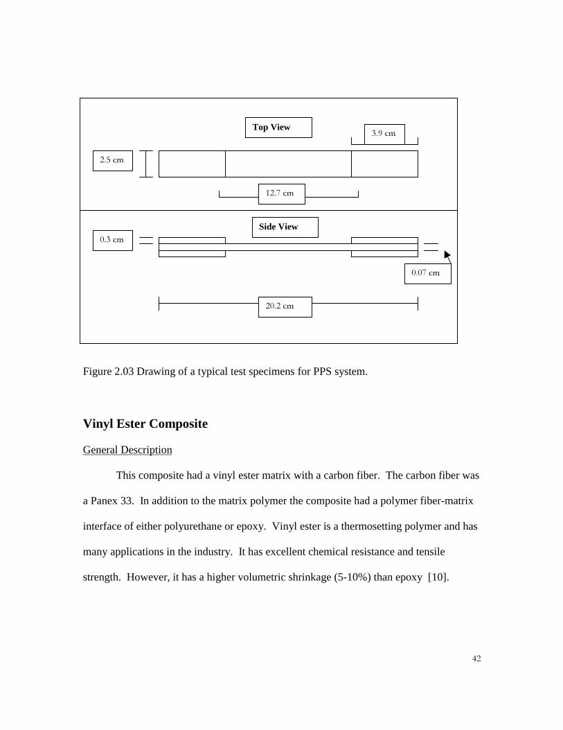
Figure 2.03 Drawing of a typical test specimens for PPS system.

Vinyl Ester Composite

General Description

This composite had a vinyl ester matrix with a carbon fiber. The carbon fiber was

a Panex 33. In addition to the matrix polymer the composite had a polymer fiber-matrix

interface of either polyurethane or epoxy. Vinyl ester is a thermosetting polymer and has

many applications in the industry. It has excellent chemical resistance and tensile

strength. However, it has a higher volumetric shrinkage (5-10%) than epoxy [10].

Top View

Side View

�����FP

�����FP

����FP

����FP

����FP

�����FP

��

Processing

Dow Chemical Company supplied the vinyl ester matrix polymer. The matrix

material consisted of 70 weight percent of pure vinyl ester and 30 percent of styrene

monomer. The vinyl ester (Tg of 140 degrees C) had an average molecular weight (Mn)

of 680 g/mol and was terminated by a methacrylate functional group. The fiber-matrix

interface material was obtained from B.F. Goodrich and is refered to as SANCURE 2026

(polyurethane). The other fiber-matrix interface material was a priority Z’ epoxy treated

fiber.

The composite was manufactured by pultrusion at Strongwell, Inc. using their

pilot scale pultruder. Spools of carbon fibers were placed in the creel rack for its

processing. The individual tows were directed into the process on a teflon board. The

fibers were dipped in the resin bath and cured at 150 degrees C.

Specimen Preparation

This material was in limited supply because it was being used on another project.

However one 8-foot strip was supplied of each epoxy and polyurethane fiber-matrix

interfaces. The strip was cut into twelve 8-inch specimens for each of the fiber-matrix

interfaces. Aluminum end tabs with a steel screen system were employed. This system

is not the traditional tabbing method based on ASTM Standards [12]. However, it was

found to be an effective tabbing system that did not allow slipping or splitting.

Extensometer tabs were placed in the center of the specimen. The specimen was

then placed in the MTS using a grip pressure of 750 (psi). The extensometer was

calibrated and placed on the specimen. The heater chamber was placed around the

��

specimen and the desired elevated temperature was obtained. After the chamber was at

the desired temperature, the specimen was left in the environment for 10 minutes before

testing. The test was started with the specimen still in the environment. A typical

specimen is shown in Figure 2.04.

Top View

Side View

11.7 cm

20.2 cm

2.5 cm

Aluminum-SteelScreen Tab

4.3 cm

4.3 cm

0.074 cm

0.188 cm

Figure 2.04 Drawing of a typical test specimen for vinyl ester system.

Polyether Ether Ketone (PEEK ) Composite

General Description

This material was purchased from FiberRite Company in a prepreg form. The

prepreg contained the PEEK resin and the AS-4 carbon fiber. Three 10 inch by 10 inch

panels were produced in a hot platen vacuum press. The panels were all unidirectional

��

consisting of eight plies. PEEK is a themoplastic polymer and has many uses in

structures. PEEK is a leading thermoplastic choice to replace epoxies in some aerospace

industry applications. It has a high fracture toughness and a low water absorption [10].

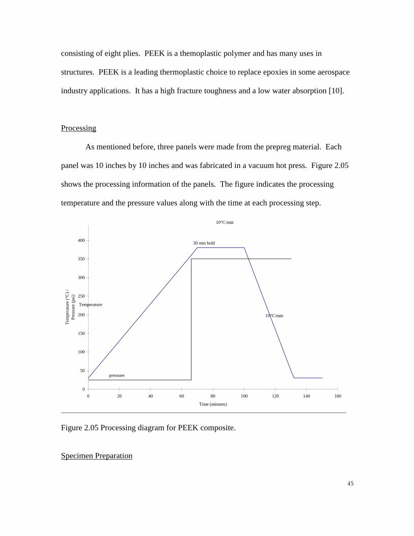
Processing

As mentioned before, three panels were made from the prepreg material. Each

panel was 10 inches by 10 inches and was fabricated in a vacuum hot press. Figure 2.05

shows the processing information of the panels. The figure indicates the processing

temperature and the pressure values along with the time at each processing step.

30 min hold

10°C/min

10°C/min

Temperature

pressure

0

50

100

150

200

250

300

350

400

0 20 40 60 80 100 120 140 160

Time (minutes)

Tem

pera

ture

(°C

) /

Pre

ssur

e (p

si)

Figure 2.05 Processing diagram for PEEK composite.

Specimen Preparation

��

After the panel was fabricated, each panel was tabbed with the glass epoxy

tabbing material. The 2.25-inch tabs were fixated to the panel with an epoxy adhesive on

both ends with the composite sandwiched between them. The adhesive then was cured at

50 degrees Celsius for 2 hours. After the panel was tabbed, the 0.5-inch wide specimens

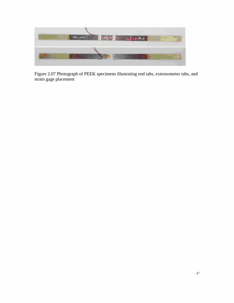
were cut from the panel. A typical specimen is shown in Figure 2.06 and 2.07.

Extensometer tabs and strain gages were then placed in the center of each specimen. The

strain gages were supplied by Micro-Measurements Group, Inc. and were of type CEA-

06-125UW-350. They were mounted on the specimens using M-Bond 600 by the

directions given by Micro-Measurements. The specimens were then placed in the MTS

grips and the heat environment was applied for 10 minutes before the test began.

Figure 2.06 Dimensional drawling of PEEK specimens.

Top View

Side View

������FP

�����FP

������FP

�����FP

����FP

������FP

��

Figure 2.07 Photograph of PEEK specimens illustrating end tabs, extensometer tabs, andstrain gage placement

��

III. Experimental Results and Discussion

Polyphenylene Sulfide (PPS) Composite

Fiber Volume Fraction

Table 3.01 Results of the fiber volume fracture measurements for PPS matrix composite.

Specimen # Dry Weight (gr.) Wet Weight (gr.) Density ofComposite

Volume Fractionof Fiber

1 0.3613 0.1748 1.5149 0.39752 0.2843 0.1370 1.5093 0.38483 0.3494 0.1684 1.5096 0.38534 0.3130 0.1511 1.5118 0.39055 0.4152 0.2008 1.5144 0.39636 0.2990 0.1444 1.5124 0.3918

As shown is Table 3.01, the fiber volume fraction for the PPS matrix composite

was measured to be, on average 39 percent. This is the average value from the six

independent specimens shown in Table 3.01.

XPS

The surface chemistry was analyzed with an X-ray Photoelectron Spectroscopy

(XPS) presented the following elements: Carbon 1s 81.23%, Oxygen 1s 10.16%, Sulfur

2p 4.93%, Silicone 2p 2.11%, Sodium1s 0.33%, Nitrogen 1s 0.92%, Chloride 2p 0.31%.

These are expected elements to be found in a PPS composite. Chloride is a typical

element used in formulation of the PPS polymer.

��

DMA

The results from the DMA indicate that the glass transition temperature for the

PPS composite is 128 degrees Celsius. This value is greater than the bulk PPS glass

transition temperature of 88 degrees Celsius. However, a composite is different from the

bulk matrix material because the carbon fibers can influence this test and the state of the

matrix material. The results from the DMA are shown in Figure 3.01.

Figure 3.01 DMA Result for PPS matrix composite system.

��

Results of Macro-Mechanical Test

All one hundred and twenty six plus specimens were tested for ultimate strength

on an MTS hydraulic closed loop axial loading machine with loading rates of 40 lbf/sec,

50 lbf/sec, and 150 lbf/sec. Each specimen had the same nominal cross sectional area.

Stress and strain were measured in the fiber direction. The stress was calculated

by dividing the load by the cross-sectional area. The strain was measured, the majority of

the time, using an extensometer supplied by MTS. MTS rated the extensometer to be

calibrated to 300 degrees Fahrenheit (or 150 degrees Celsius). This was verified using an

extensometer measurement on a piece of steel at the elevated temperatures. Strain gages

were also used on some specimens to compare with the extensometer.��The measured

modulus of the steel was 31 (Msi). This is a little high from the standard value of 30

(Msi) for steel; however, this measurement was consistent in the temperature range. The

load cell for this MTS may need to be calibrated.

Stress-strain curves were generated to determine young’s modulus (stiffness) of

the composite. The moduli were measured on the linear domain of the curve. This

domain included approximently 40% or 50% of failure strength. Typical stress-strain

curves, for the PPS composite system, are given in Figures 3.02 and 3.03.

��

PPS Composite at 33.4 degrees C/ I.D. # ws-81ss

0

50

100

150

200

250

300

0 0.005 0.01 0.015 0.02 0.025

Strain (in/in)

Str

ess

(ksi

)

Extensometer measurement

Strain gage measurement

Young’s Modulus (Strain Gage)= 12.31 x10^6 psiYoung’s Modulus (Extensometer= 12.06 x10^6 psi

Figure 3.02 Stress-strain calibration of extensometer with strain gage strainmeasurements.

Figure 3.02 demonstrates the calibration efforts on the extensometer. On this

particular specimen strain was measured in the fiber direction with both an extensometer

and a strain gage. The strain gage produced a modulus of 12.31 msi; the extensometer

produced a modulus of 12.06 msi. Furthermore, calibration tests were conducted

measuring the strain with the extensometer on a piece of steel at elevated temperatures.

The results of this particular calibration test do not appear in this work. However, the

results of the calibration tests were satisfactory. Therefore, the extensometer is an

appropriate device to measure the strain between the temperatures of 300 to 1500 Celsius.

��

PPS from PCI at 69.9 degrees C/ ID # ws-718a

0

50

100

150

200

250

0 0.005 0.01 0.015 0.02 0.025

Strain (in)

Str

ess

(ksi

)

Young’s Modulus12.584 x 10^6 psi

Ultimate Stress232.685 ksi

Figure 3.03 Stress-strain curve for PPS composite material.

Table 3.02 and Figure 3.04 give the statistical results for all tests run at that

temperature. This includes all three major loading rates.

Table 3.02 Results from all PPS Composite (PCI) tension tests- @ all loading rates.

7HVW7HPSHUDWXUH

�&��

��RI6SHFLPHQV�$OO�ORDGUDWH�

$YHUDJH6WUHQJWK�NVL�

6WDQGDUG'HYLDWLRQ�IRU

6WUHQJWK

$YHUDJH<RXQJV0RGXOXV�[��A��SVL�

6WDQGDUG'HYLDWLRQ�IRU

<RXQJV0RGXOXV

�� �� ����� ���� ������ ������� �� ����� ���� ������ ������� �� ����� ���� ������ ������� �� ����� ���� ������ ������� �� ����� ���� ������ �������� �� ����� ���� ������ �������� �� ����� ���� ������ �������� �� ����� ���� ������ �������� �� ����� ���� ������ �������� �� ����� ���� ������ �������� �� ����� ���� ������ �����

��

Strength of PPS Carbon Fiber Composite

0

50

100

150

200

250

300

0 20 40 60 80 100 120 140 160

Temperature (C)

Str

eng

th (

ksi)

12 specimens at each temp.

Literature Bulk PPS Tg Temp. DMA Tg for PPS Composite

Figure 3.04 A plot of the strength values for the PPS Composite material with theirrespective temperatures with standard deviations as error bars.

As we can see (in Figure 3.04) the average strength of this composite can be

expected to decline 17.7 percent from 300 to 1400 Celsius. In addition to this decline in

strength, the data indicate that the strength declines both at 90 and 130 degrees Celsius.

These temperatures are unique to the material because 90 degrees Celsius is the literature

value for the glass transitional temperature for bulk PPS, and 126 degrees is the measured

(by DMA) glass transition temperature for the PPS composite system. Figure 3.04

indicates both of these transitions. One possible explanation to these two transitions is

that the bulk matrix away from the fibers is changing at 90 degrees Celsius. Then the

matrix material near the fibers is changed at 130 degrees Celsius.

��

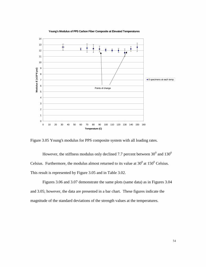
Young’s Modulus of PPS Carbon Fiber Composite at Elevated Temperatures

0

1

2

3

4

5

6

7

8

9

10

11

12

13

14

0 10 20 30 40 50 60 70 80 90 100 110 120 130 140 150 160

Temperature (C)

Mo

du

lus

E (

x10^

6 p

si)

8 specimens at each temp.

Points of change

Figure 3.05 Young’s modulus for PPS composite system with all loading rates.

However, the stiffness modulus only declined 7.7 percent between 300 and 1300

Celsius. Furthermore, the modulus almost returned to its value at 300 at 1500 Celsius.

This result is represented by Figure 3.05 and in Table 3.02.

Figures 3.06 and 3.07 demonstrate the same plots (same data) as in Figures 3.04

and 3.05; however, the data are presented in a bar chart. These figures indicate the

magnitude of the standard deviations of the strength values at the temperatures.

��

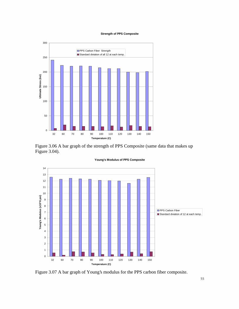
Strength of PPS Composite

0

50

100

150

200

250

300

32 60 70 80 90 100 110 120 130 140 150

Temperature (C)

Ult

imat

e S

tres

s (k

si)

PPS Carbon Fiber Strength

Standard diviation of all 12 at each temp.

Figure 3.06 A bar graph of the strength of PPS Composite (same data that makes upFigure 3.04).

Young’s Modulus of PPS Composite

0

1

2

3

4

5

6

7

8

9

10

11

12

13

14

32 60 70 80 90 100 110 120 130 140 150

Temperature (C)

Yo

un

g’s

Mo

du

lus

(x10

^6 p

si)

PPS Carbon Fiber

Standard diviation of 12 at each temp.

Figure 3.07 A bar graph of Young’s modulus for the PPS carbon fiber composite.

��

All of the above data were evaluated with all three loading rates. This testing was

intended to explore the visco-elastic properties of composites. The combination of

different strain rates and elevated temperatures may influence the strength of the

composite. This behavior was interrogated using different loading rates on the material at

the temperatures. The results are given in Figure 3.08.

Strength of PPS (PCI) at Different Loading Rates

0

50000

100000

150000

200000

250000

300000

0 50 100 150 200 250 300 350 400

Temperature (F)

Ult

imat

e S

tren

gth

(p

si)

50 lbf/sec

40 lbf/sec

150 lbf/sec

Figure 3.08 The strength of PPS composite differentiating load rates of 40,50, and 150pounds per sec.

The visco-elastic response is difficult to explore. For amorphous polymers, the

principles of linear viscoelasticity can be applied. However for semi-crystalline polymers

these techniques can not be applied. Semi-crystalline polymers maintain a higher

modulus over a wider range of temperatures. Additionally, the fiber dominance of this

system may off set any visco-elastic response. A difference in strength is seen between

��

the rates of 40 and 50 pounds per second. However, the rate of 150 lbf/sec is within the

scatter of 40 and 50 lbf/sec.

In addition to the above data points, more data were collected on strength at

higher temperatures. Only the strength was collected at these temperatures because they

were beyond the range of the extensometer. Figure 3.09 reports points above 150 degrees

Celsius.

Strength for PPS Composite (PCI) at Elevated Temperatures

0

50000

100000

150000

200000

250000

300000

0 50 100 150 200 250

Temperature (C)

Str

eng

th (

psi

)

All PPS Strength data

Bulk PPS Melt Temp.

Figure 3.09 All strength data on PPS composite, data without strain measurements.

The strength does not appear to decline dramatically as the melt temperature for

PPS is approached. The melt temperature for bulk PPS is approximately 285 degrees

Celsius. However, the strength may have a dramatic decline as the test temperature

��

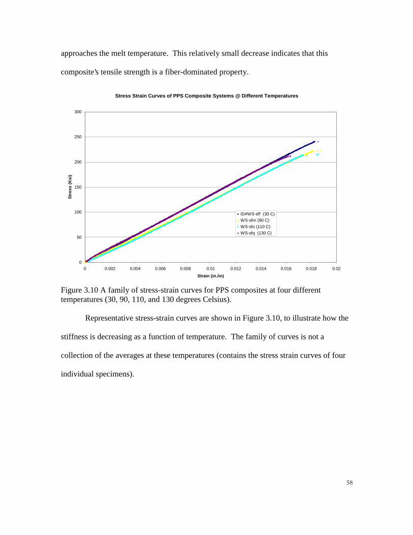
approaches the melt temperature. This relatively small decrease indicates that this

composite’s tensile strength is a fiber-dominated property.

Stress Strain Curves of PPS Composite Systems @ Different Temperatures

0

50

100

150

200

250

300

0 0.002 0.004 0.006 0.008 0.01 0.012 0.014 0.016 0.018 0.02

Strain (in./in)

Str

ess

(Ksi

)

ID#WS-sff (30 C)

WS-sfm (90 C)

WS-sfo (110 C)

WS-sfq (130 C)

Figure 3.10 A family of stress-strain curves for PPS composites at four differenttemperatures (30, 90, 110, and 130 degrees Celsius).

Representative stress-strain curves are shown in Figure 3.10, to illustrate how the

stiffness is decreasing as a function of temperature. The family of curves is not a

collection of the averages at these temperatures (contains the stress strain curves of four

individual specimens).

��

P.C.I. PPS Matrix-Carbon Fiber Composite, Strength Unidirectional Tension

0

50000

100000

150000

200000

250000

300000

-250 -200 -150 -100 -50 0 50 100 150 200 250

Temperature (C)

Str

eng

th (

psi

)

P.C.I. PPS [0]

Figure 3.11 Strength of PPS composite at elevated temperatures and cryogenictemperatures.

In addition to the elevated temperature tests, the system was also evaluated at

cryogenic temperatures. The evaluation was not as extensive as the elevated

temperatures; nevertheless, some data was obtained (Figure 3.11). It appears that the PPS

composite gains strength at cryogenic temperatures when compared to room temperature

strength values. No strain measurements were made of the cryogenically tested

specimens. Future testing should be conducted in this area.

Fracture Modes

The failure mode for the PPS composite was of the type XGM (X-explosive, G-

gage, M-middle) according to the ASTM Standards D 3039 [12]. They had excessive

��

longitudinal splitting making the failure surfaces highly irregular and jagged. These

types of failures are sometimes defined as being a “plastic” failure. Plastic failure occurs

when the fiber debonds from the matrix prior to overall failure of the composite. The

failures of two specimens are shown in Figure 3.12 and Figure 3.13. Figure 3.12 shows

the failure at 31.1 degrees Celsius and Figure 3.13 shows the failure at 229 degrees

Celsius. At the elevated temperature, the matrix appears to be curling or pealing back at

failure.

Figure 3.12 Fracture of PPS specimen at 31.1 degrees Celsius (Front and Side Views).

��

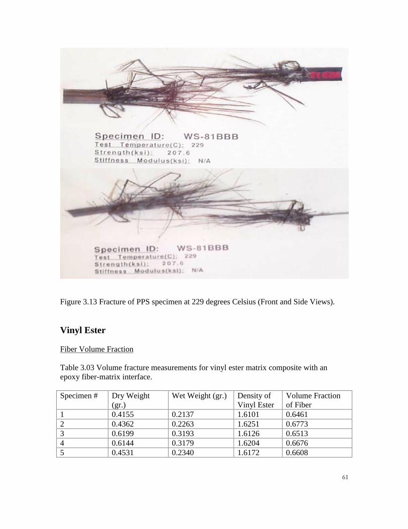
Figure 3.13 Fracture of PPS specimen at 229 degrees Celsius (Front and Side Views).

Vinyl Ester

Fiber Volume Fraction

Table 3.03 Volume fracture measurements for vinyl ester matrix composite with anepoxy fiber-matrix interface.

Specimen # Dry Weight(gr.)

Wet Weight (gr.) Density ofVinyl Ester

Volume Fractionof Fiber

1 0.4155 0.2137 1.6101 0.64612 0.4362 0.2263 1.6251 0.67733 0.6199 0.3193 1.6126 0.65134 0.6144 0.3179 1.6204 0.66765 0.4531 0.2340 1.6172 0.6608

��

As shown in Table 3.03, the average percent fiber in the Vinyl Ester Composite

was 66 percent. This is for the vinyl ester composite with the epoxy fiber-matrix

interface. Fiber volume fraction tests were not preformed on the vinyl ester composite

with a polyurethane fiber-matrix interface because the both composite systems were

products of the same pultrution method. Also for this calculation the composite was

assumed to consist of only vinyl ester and carbon fiber (no interphase effect was

included). The fiber-matrix interface material should be in low concentrations.

Therefore, the percent fiber volume fraction should be the same for both systems.

Results of Macro-Mechanical Test

In addition to the PPS composite system, a thermosetting plastic matrix was

studied at elevated temperatures. The matrix is made of vinyl ester with two different

fiber-matrix interfaces, epoxy and polyurethane. Epoxy is a thermosetting polymer and

polyurethane is a thermoplastic. The fiber is made of carbon, however, it was not

determined what specific type of fiber was in the composite. Only some statistical

analysis was determined for this composite system because the supply of material was

low (Tables 3.04 and 3.05).

Table 3.04 Strength and stiffness results of vinyl ester composite with an epoxy fiber-matrix interface.TestTemperature(C)

# ofSpecimens

AverageStrength(ksi)

StandardDeviationfor Strength

AverageStiffness(x10^6 psi)

StandardDeviationfor Stiffness

35 2 109.5 12.1 16.23 070 2 106.3 1.90 14.66 090 2 101.8 3.80 15.39 0.62110 2 89.0 0.99 14.40 0.40130 1 83.6 N/A 14.60 N/A140 1 76.1 N/A 14.60 N/A-123.3 1 131.5 N/A N/A N/A

��

Table 3.05 Strength and stiffness results of vinyl ester composite with a polyurethanefiber-matrix interface.TestTemperature(C)

# ofSpecimens

AverageStrength(ksi)

StandardDeviationfor Strength

AverageStiffness(x10^ psi)

StandardDeviationfor Stiffness

34 2 160.3 1.11 18.1 0.5090 1 124.8 N/A 17.1 N/A110 1 129.9 N/A 16.8 N/A130 1 121.7 N/A 16.3 N/A150 1 108.8 N/A N/A N/A-189.4 3 175.6 8.83 18.7 0.65-101.0 1 156.0 N/A 17.7 N/A

�Figures 3.14 and 3.15 show a typical stress-strain curve for the vinyl ester system.

The strain was measured by the extensometer for all of the specimens in this family. The

stiffness of young’s modulus was measured from the stress strain curve using the slope of

the curve up to 40 percent of the failure strength.

Vinyl Ester with Polyurethane interface @ 109.3 degrees C/ ID # ve-pud

0

20

40

60

80

100

120

140

0 0.001 0.002 0.003 0.004 0.005 0.006 0.007 0.008 0.009 0.01

Strain (in/in)

Str

ess

(ksi

)

Young’s Modulus16.773 x 10^6 psi

Ultimate Stress129.861 ksi

Figure 3.14: Stress-strain curve for vinyl ester with polyurethane interface.

��

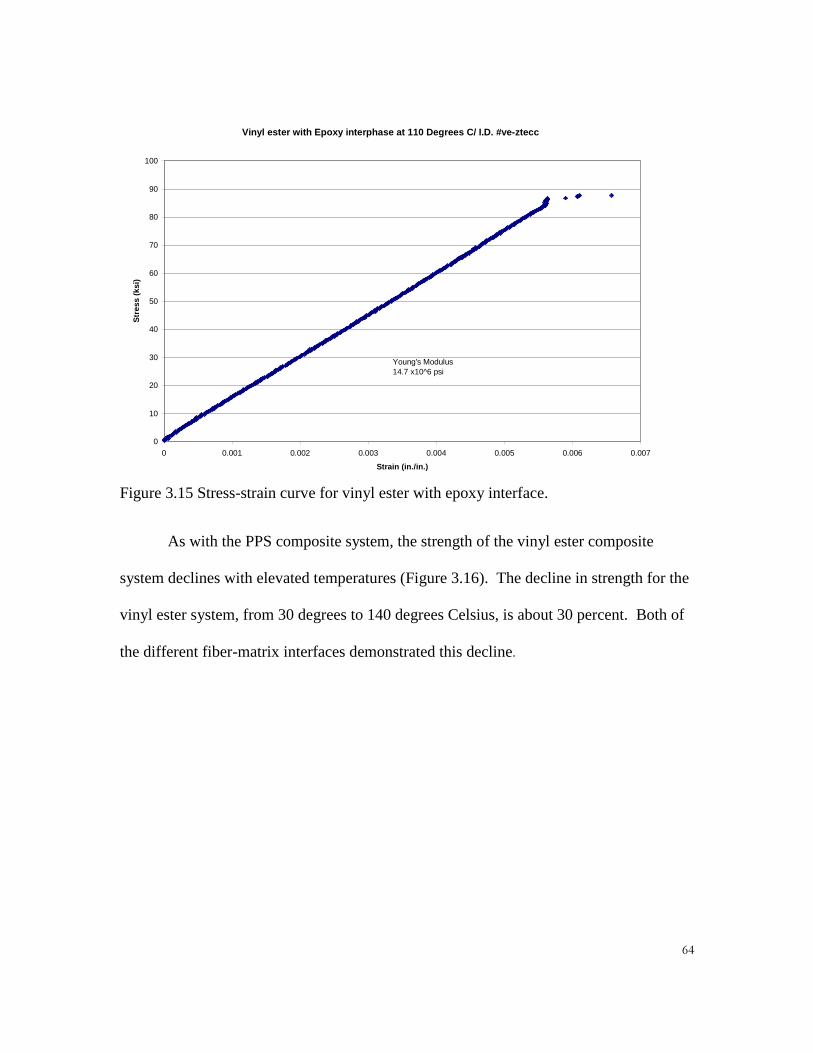
Vinyl ester with Epoxy interphase at 110 Degrees C/ I.D. #ve-ztecc

0

10

20

30

40

50

60

70

80

90

100

0 0.001 0.002 0.003 0.004 0.005 0.006 0.007

Strain (in./in.)

Str

ess

(ksi

)

Young’s Modulus14.7 x10^6 psi

Figure 3.15 Stress-strain curve for vinyl ester with epoxy interface.

As with the PPS composite system, the strength of the vinyl ester composite

system declines with elevated temperatures (Figure 3.16). The decline in strength for the

vinyl ester system, from 30 degrees to 140 degrees Celsius, is about 30 percent. Both of

the different fiber-matrix interfaces demonstrated this decline�

��

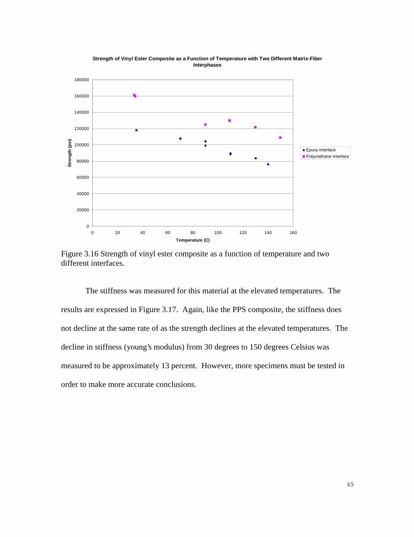
Strength of Vinyl Ester Composite as a Function of Temperature with Two Different Matrix-Fiber Interphases

0

20000

40000

60000

80000

100000

120000

140000

160000

180000

0 20 40 60 80 100 120 140 160

Temperature (C)

Str

eng

th (

psi

)

Epoxy Interface

Polyurethane Interface

Figure 3.16 Strength of vinyl ester composite as a function of temperature and twodifferent interfaces.

The stiffness was measured for this material at the elevated temperatures. The

results are expressed in Figure 3.17. Again, like the PPS composite, the stiffness does

not decline at the same rate of as the strength declines at the elevated temperatures. The

decline in stiffness (young’s modulus) from 30 degrees to 150 degrees Celsius was

measured to be approximately 13 percent. However, more specimens must be tested in

order to make more accurate conclusions.

��

Young’s Modulus for Vinyl Ester with Two Different Matrix-Fiber Interphases

0

2

4

6

8

10

12

14

16

18

20

0 20 40 60 80 100 120 140 160

Temperature (C)

Yo

un

g’s

Mo

du

lus

(x10

^6 p

si)

Epoxy Interface

Polyurethane Interface

Figure 3.17 Stiffness of vinyl ester composite as a function of temperature and twodifferent interfaces.

Representative stress-strain curves are shown in Figure 3.18. This figure shows

the strength and stiffness changes as a function of temperature. This figure illustrates that

temperature does not effect the elastic region of the stiffness; however, the temperature

effect is in the inelastic region.

��

Stress Strain Curves For Vinyl Ester with Epoxy Fiber Matrix Interface @ Elevated Temperatures

0

20

40

60

80

100

120

140

0 0.001 0.002 0.003 0.004 0.005 0.006 0.007 0.008 0.009 0.01

Strain (in/in)

Str

ess

(ksi

)

ID#ve-ztecc (110 C)

ID#ve-ztecd (130 C)

ID#ve-ztedf (35 C)

ID#ve-ztece (140 C)

ID#ve-ztecb (90 C)

Figure 3.18 A family of stress-strain curves for vinyl ester composite with an epoxyfiber-matrix interface at different temperatures (90, 140,35,110, and 130 Degrees C).

In addition to the elevated temperature strength values, cryogenic temperature

tests were conducted on the vinyl ester system. As with the PPS system, the strength of

the system appears to increase at the cryogenic temperatures compared with the room

temperature values. The results of these tests are added to the elevated temperature

results and shown in Figure 3.19.

��

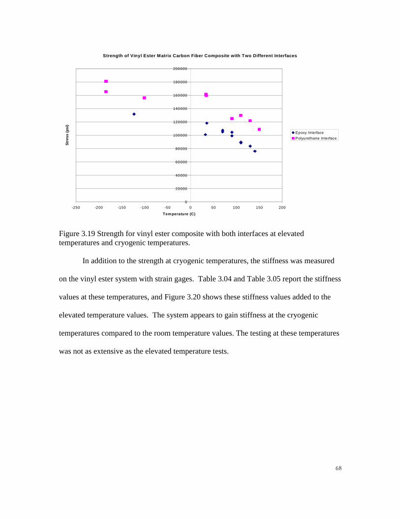
Strength of Vinyl Ester Matrix Carbon Fiber Composite with Two Different Interfaces

0

20000

40000

60000

80000

100000

120000

140000

160000

180000

200000

-250 -200 -150 -100 -50 0 50 100 150 200

Temperature (C)

Str

ess

(psi

)

Epoxy Interface

Polyurethane Interface

Figure 3.19 Strength for vinyl ester composite with both interfaces at elevatedtemperatures and cryogenic temperatures.

In addition to the strength at cryogenic temperatures, the stiffness was measured

on the vinyl ester system with strain gages. Table 3.04 and Table 3.05 report the stiffness

values at these temperatures, and Figure 3.20 shows these stiffness values added to the

elevated temperature values. The system appears to gain stiffness at the cryogenic

temperatures compared to the room temperature values. The testing at these temperatures

was not as extensive as the elevated temperature tests.

��

Stiffness of a Vinyl Ester Carbon Fiber with Two Different Fiber-Matrix Interfaces Composite

0

5

10

15

20

25

-250 -200 -150 -100 -50 0 50 100 150 200

Temperature (C)

Sti

ffn

ess

(x10

^6 p

si)

Epoxy Interface

Polyurethane Interface

Figure 3.20 Stiffness values of the vinyl ester composite with both fiber-matrix interfacesat elevated temperature and cryogenic temperatures.

Fracture Modes

The failure mode for both vinyl ester systems were characterized as type XGM

(X-explosive, G-gage, M-middle) according to the ASTM Standard D 3039/D 3039M-93

[12]. The vinyl ester system with the polyurethane fiber-matrix interface offers a failure

mode change. This is shown in Figure 3.21 to Figure 3.22. The room temperature failure

(Figure 3.21) has splitting of the matrix with clumps of fiber. However the failure at 150

degrees Celsius (Figure 3.22) is more of a "fluffy" failure of the composite. In

explanation of this difference, the elevated temperature appears to be debonding from the

fibers. At lower temperatures a more brittle failure in the matrix occurs making the

��

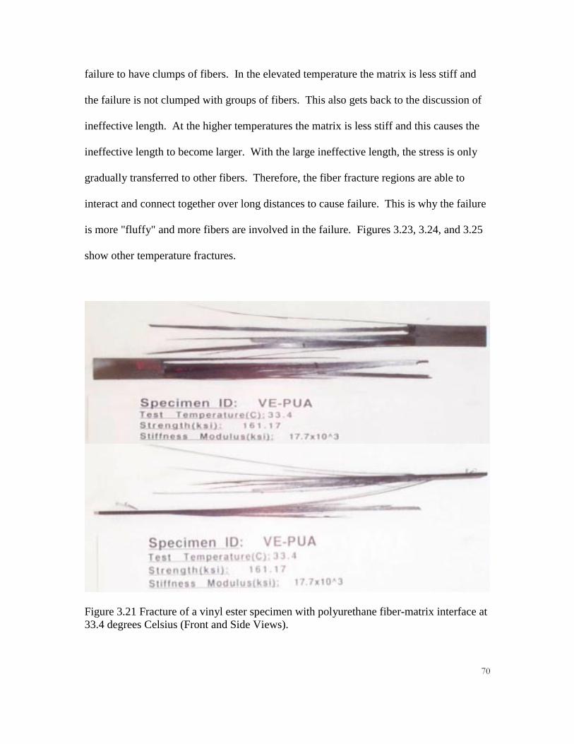
failure to have clumps of fibers. In the elevated temperature the matrix is less stiff and

the failure is not clumped with groups of fibers. This also gets back to the discussion of

ineffective length. At the higher temperatures the matrix is less stiff and this causes the

ineffective length to become larger. With the large ineffective length, the stress is only

gradually transferred to other fibers. Therefore, the fiber fracture regions are able to

interact and connect together over long distances to cause failure. This is why the failure

is more "fluffy" and more fibers are involved in the failure. Figures 3.23, 3.24, and 3.25

show other temperature fractures.

Figure 3.21 Fracture of a vinyl ester specimen with polyurethane fiber-matrix interface at33.4 degrees Celsius (Front and Side Views).

��

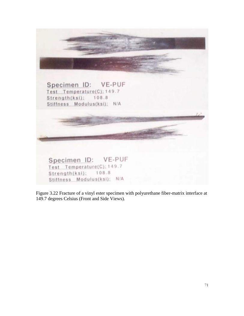
Figure 3.22 Fracture of a vinyl ester specimen with polyurethane fiber-matrix interface at149.7 degrees Celsius (Front and Side Views).

��

Figure 3.23 Fracture of a vinyl ester specimen with polyurethane fiber-matrix interface at-184.4 degrees Celsius (Front and Side Views).

��

Figure 3.24 Fracture of a vinyl ester specimen with epoxy fiber-matrix interface at 35degrees Celsius (Front and Side Views).

��

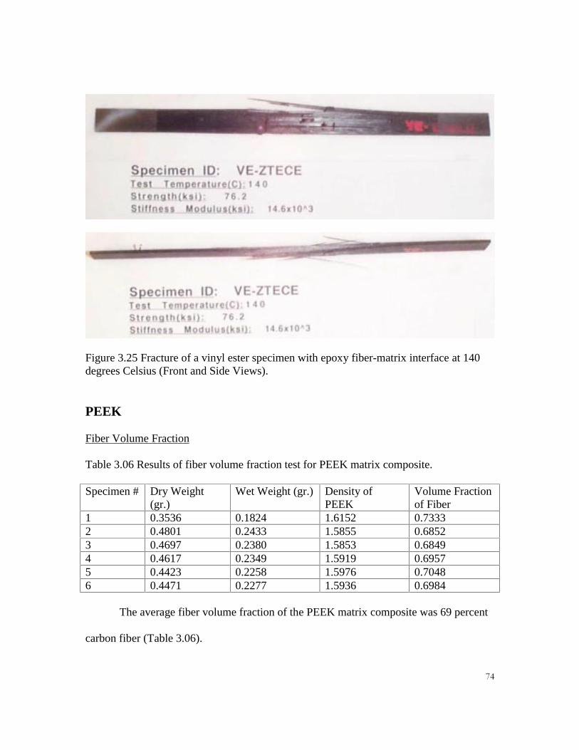
Figure 3.25 Fracture of a vinyl ester specimen with epoxy fiber-matrix interface at 140degrees Celsius (Front and Side Views).

PEEK

Fiber Volume Fraction

Table 3.06 Results of fiber volume fraction test for PEEK matrix composite.

Specimen # Dry Weight(gr.)

Wet Weight (gr.) Density ofPEEK

Volume Fractionof Fiber

1 0.3536 0.1824 1.6152 0.73332 0.4801 0.2433 1.5855 0.68523 0.4697 0.2380 1.5853 0.68494 0.4617 0.2349 1.5919 0.69575 0.4423 0.2258 1.5976 0.70486 0.4471 0.2277 1.5936 0.6984

The average fiber volume fraction of the PEEK matrix composite was 69 percent

carbon fiber (Table 3.06).

��

C-Scans Results

The C-Scan was nondestructive evaluation used to detect any major flaws in the

panel formation. Three 10 inch by 10 inch panels were C-Scanned for flaws. No

detectable flaws were found in any of the panels. Figure 3.26 is an example of a C-Scan

on one of the panels.

Figure 3.26 C-Scan of PEEK matrix composite.

Results of Macro-Mechanical Test

Thirty specimens were tested for ultimate strength on the MTS at a loading rate of

50 lb./sec. Strain was also measured for many of the specimens with both a strain gage

and an extensometer. The stiffness was measured on the linear domain of the stress-

strain curve. This slope was calculated up to approximently 50 % of the failure strength.

The results of this analysis are given in Table 3.07.

��

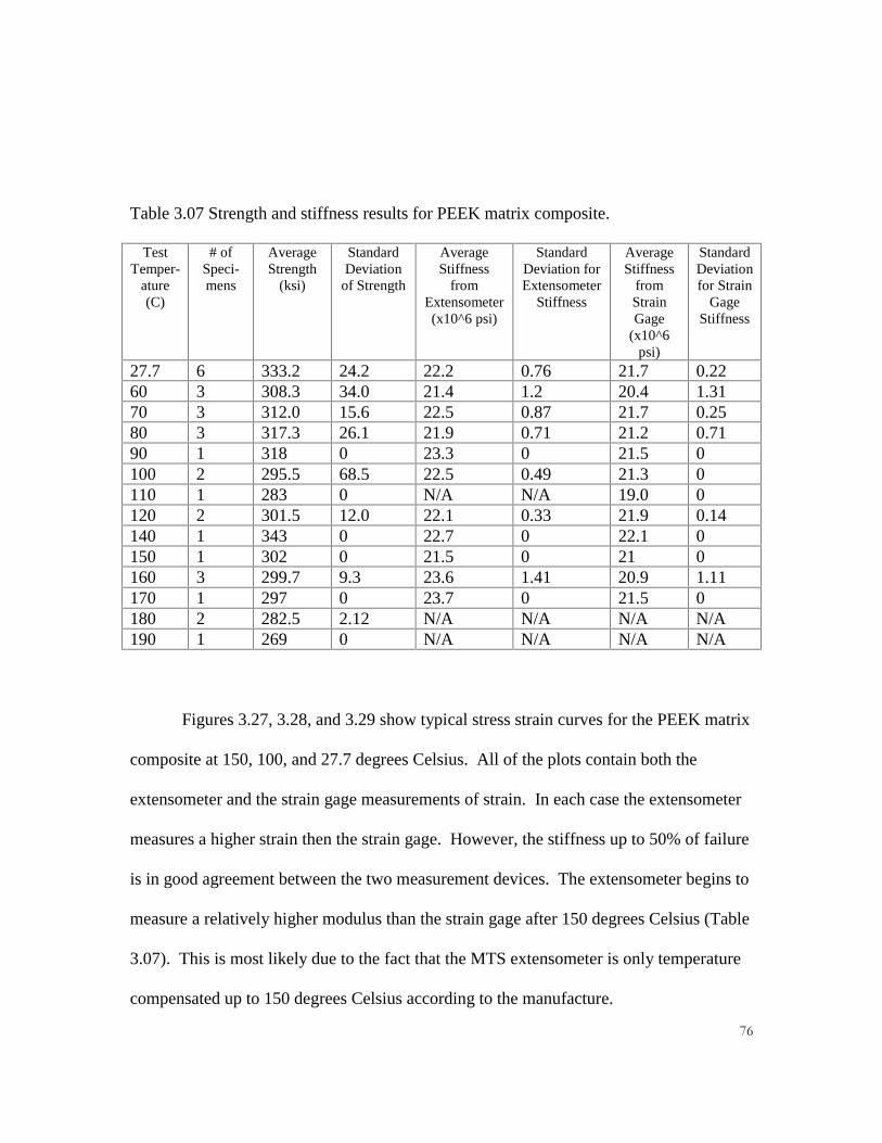
Table 3.07 Strength and stiffness results for PEEK matrix composite.

TestTemper-

ature(C)

# ofSpeci-mens

AverageStrength

(ksi)

StandardDeviation

of Strength

AverageStiffness

fromExtensometer(x10^6 psi)

StandardDeviation forExtensometer

Stiffness

AverageStiffness

fromStrainGage

(x10^6psi)

StandardDeviationfor Strain

GageStiffness

27.7 6 333.2 24.2 22.2 0.76 21.7 0.2260 3 308.3 34.0 21.4 1.2 20.4 1.3170 3 312.0 15.6 22.5 0.87 21.7 0.2580 3 317.3 26.1 21.9 0.71 21.2 0.7190 1 318 0 23.3 0 21.5 0100 2 295.5 68.5 22.5 0.49 21.3 0110 1 283 0 N/A N/A 19.0 0120 2 301.5 12.0 22.1 0.33 21.9 0.14140 1 343 0 22.7 0 22.1 0150 1 302 0 21.5 0 21 0160 3 299.7 9.3 23.6 1.41 20.9 1.11170 1 297 0 23.7 0 21.5 0180 2 282.5 2.12 N/A N/A N/A N/A190 1 269 0 N/A N/A N/A N/A

Figures 3.27, 3.28, and 3.29 show typical stress strain curves for the PEEK matrix

composite at 150, 100, and 27.7 degrees Celsius. All of the plots contain both the

extensometer and the strain gage measurements of strain. In each case the extensometer

measures a higher strain then the strain gage. However, the stiffness up to 50% of failure

is in good agreement between the two measurement devices. The extensometer begins to

measure a relatively higher modulus than the strain gage after 150 degrees Celsius (Table

3.07). This is most likely due to the fact that the MTS extensometer is only temperature

compensated up to 150 degrees Celsius according to the manufacture.

��

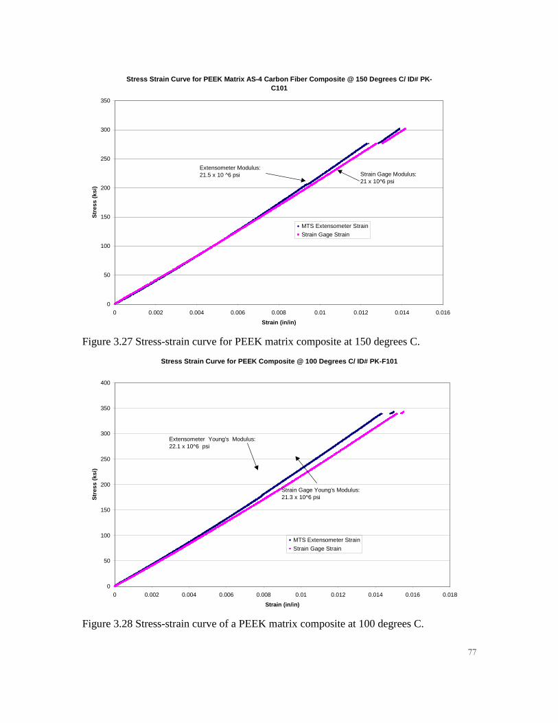
Stress Strain Curve for PEEK Matrix AS-4 Carbon Fiber Composite @ 150 Degrees C/ ID# PK-C101

0

50

100

150

200

250

300

350

0 0.002 0.004 0.006 0.008 0.01 0.012 0.014 0.016

Strain (in/in)

Str

ess

(ksi

)

MTS Extensometer Strain

Strain Gage Strain

Strain Gage Modulus:21 x 10^6 psi

Extensometer Modulus:21.5 x 10 ^6 psi

Figure 3.27 Stress-strain curve for PEEK matrix composite at 150 degrees C.

Stress Strain Curve for PEEK Composite @ 100 Degrees C/ ID# PK-F101

0

50

100

150

200

250

300

350

400

0 0.002 0.004 0.006 0.008 0.01 0.012 0.014 0.016 0.018

Strain (in/in)

Str

ess

(ksi

)

MTS Extensometer Strain

Strain Gage Strain

Extensometer Young’s Modulus:22.1 x 10^6 psi

Strain Gage Young’s Modulus:21.3 x 10^6 psi

Figure 3.28 Stress-strain curve of a PEEK matrix composite at 100 degrees C.

��

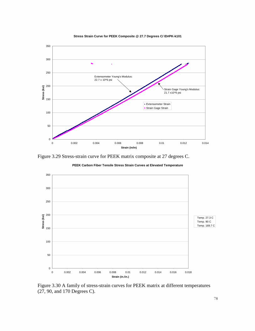
Stress Strain Curve for PEEK Composite @ 27.7 Degrees C/ ID#PK-k101

0

50

100

150

200

250

300

350

0 0.002 0.004 0.006 0.008 0.01 0.012 0.014

Strain (in/in)

Str

ess

(ksi

)

Extensometer Strain

Strain Gage Strain

Extensometer Young’s Modulus:22.7 x 10^6 psi

Strain Gage Young’s Modulus:21.7 x10^6 psi

Figure 3.29 Stress-strain curve for PEEK matrix composite at 27 degrees C.

PEEK Carbon Fiber Tensile Stress Strain Curves at Elevated Temperature

0

50

100

150

200

250

300

350

0 0.002 0.004 0.006 0.008 0.01 0.012 0.014 0.016 0.018

Strain (in./in.)

Str

ess

(ksi

)

Temp. 27.3 C

Temp. 90 C

Temp. 169.7 C

Figure 3.30 A family of stress-strain curves for PEEK matrix at different temperatures(27, 90, and 170 Degrees C).

��

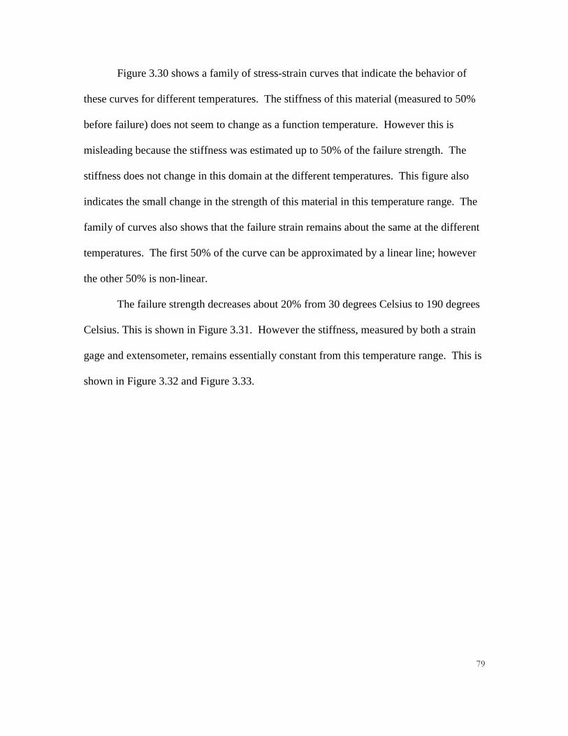
Figure 3.30 shows a family of stress-strain curves that indicate the behavior of

these curves for different temperatures. The stiffness of this material (measured to 50%

before failure) does not seem to change as a function temperature. However this is

misleading because the stiffness was estimated up to 50% of the failure strength. The

stiffness does not change in this domain at the different temperatures. This figure also

indicates the small change in the strength of this material in this temperature range. The

family of curves also shows that the failure strain remains about the same at the different

temperatures. The first 50% of the curve can be approximated by a linear line; however

the other 50% is non-linear.

The failure strength decreases about 20% from 30 degrees Celsius to 190 degrees

Celsius. This is shown in Figure 3.31. However the stiffness, measured by both a strain

gage and extensometer, remains essentially constant from this temperature range. This is

shown in Figure 3.32 and Figure 3.33.

��

Failure Strength of PEEK Carbon Fiber Composites at Elevated Temperatures

0

50

100

150

200

250

300

350

400

0 20 40 60 80 100 120 140 160 180 200

Temperature (C)

Str

eng

th (

ksi)

Figure 3.31 Strength values of PEEK matrix composite at elevated temperatures.

Extensometer Strain Measurement of Stiffness of PEEK Composite

0

5

10

15

20

25

30

0 20 40 60 80 100 120 140 160 180

Temperature (C)

Sti

ffn

ess

(x10

^6 p

si)

Figure 3.32 Stiffness values for PEEK matrix composite measured with an extensometer.

��

Strain Gage Measurement of Stiffness of PEEK Composite

0

5

10

15

20

25

0 20 40 60 80 100 120 140 160 180

Temperature (C)

Sti

ffn

ess

(x10

^6 p

si)

Figure 3.33 Stiffness of PEEK matrix composite measured with a strain gage.

The average strength and the standard deviation of these values are shown in

Figure 3.34. This data set is not as extensive as the PPS system; however, it is more

extensive than the vinyl ester set. The deviation at the lower temperatures appears to be

more extensive than at the higher temperatures. However this might be just the scatter of

the material and more specimens should be tested at these temperatures for the complete

picture.

In addition to the strength, the average stiffness and the standard deviation of

these values are shown in Figure 3.35. This figure compares the extensometer and strain

gage strain for the stiffness calculation. As mentioned above, the extensometer measured

a higher stiffness than the strain gage.

��

Strength of PEEK Matrix at Failure at Elevated Temperatures

0

50

100

150

200

250

300

350

400

0 20 40 60 80 100 120 140 160 180 200

Temperature (C)

Str

ess

(ksi

)

Figure 3.34 Average strength of PEEK matrix composite with standard deviations.

Stiffness of PEEK Matrix Composite at Elevated Temperatures

0

5

10

15

20

25

30

0 20 40 60 80 100 120 140 160 180

Temperature (C)

Yo

un

g’s

Mo

du

lus

(x10

^6 p

si)

Extensometer Stiffness

Strain Gage Stiffness

Figure 3.35 Stiffness of PEEK matrix composite with standard deviations.

��

Fracture Modes

The failure mode for this system is not fully characterized in the ASTM

Standards. The failure was a complete "explosion" of the material. Many times after

failure the only material left in the MTS were the glass epoxy tabs in the grips. This

could be a result of the high volume fraction of fiber.

Summary of Experimental Results

The unidirectional tensile strength of the PPS composite system decreased by 17

percent from 30 degrees Celsius to 140 degrees Celsius. The unidirectional stiffness of

this same system decreased 7.7 percent between 30 and 130 degrees Celsius. These

changes appear to occur near two distinct points, at the bulk PPS glass transition

temperature and the PPS composite glass transition. The loading rate did not affect the

strength of this system over the ranges of 40 to 150 pounds per second. The strength of

the system slightly increases at -180 degrees Celsius compared to room temperature.

The unidirectional tensile strength of the vinyl ester composite with two different

fiber-matrix interfaces decreased by 30 percent from 30 to 140 degrees Celsius. The

unidirectional stiffness of these systems decreased by 13 percent from 30 to 150 degrees

Celsius. The strength of those systems slightly increased at -180 degrees Celsius

compared to room temperature strength. The stiffness of the vinyl ester composite with

the polyurethane interface slightly increased at -180 degrees Celsius. A failure mode

change in the vinyl ester composite with the polyurethane interface was found between

150 and 30 degrees Celsius.

��

The unidirectional tensile strength of the PEEK composite decreased by 20

percent from 30 to 190 degrees Celsius. The unidirectional elastic stiffness was

essentially constant in this temperature range. However, the temperature did affect the

inelastic region of the stiffness for this system.

��

IV. Model Development and Prediction of ExperimentalResults

Parametric Study

In order to examine how the interfacial shear strength affects the strength of the

composite, a parametric study was preformed with the two models discussed in the

literature review. Both interfacial shear strength and the polymer shear modulus were

studied parametrically to examine how they effect the composite strength. After the

shear modulus parametric study, it was determined that this parameter does not effect the

strength of the composite as much as the interfacial shear strength effects the composite

strength. Figure 4.01 shows how the interfacial shear strength effects the strength values

as it is decreased from 8000 (psi). Typical values of the interfacial shear strength are in

this range. This parametric study did not take in account the fact that both the shear

modulus and strength are changing. However, it did demonstrate that the composite

strength, based on the models, does change by large amounts as the interfacial shear

strength is changed.

��

Figure 4.01 Parametric study of the interfacial shear strength effect on strength of acomposite.

Changes to Model Parameters for Elevated Temperature

As Figure 1.06 indicated, the interfacial shear strength should be some function of

temperature. No specific measurement was made on the interfacial shear strength with

PPS and a carbon fiber at elevated temperatures. Assuming this trend would apply to the

PPS system, an approximation was generated of the interfacial shear strength as a

function of elevated temperatures. This is shown in Figure 4.02. The approximation used

a value of room temperature interfacial shear strength for PPS with a carbon fiber found

in the literature [13]. Using the room temperature as one reference point and the melt

��

temperature of PPS as the other reference point, a straight line was fitted. At melt

temperature, the interfacial shear strength was assumed to be zero.

Calculated Interfacial Shear Strength for PPS with AS-4 Carbon Fiber

0

500

1000

1500

2000

2500

3000

3500

4000

4500

0 20 40 60 80 100 120 140 160 180

Temperature (C)

Inte

rfac

ial S

hea

r S

tren

gth

(p

si)

Figure 4.02 Approximation of the interfacial shear strength as a function of temperaturefor a PPS composite system.

In addition to the interfacial shear strength, Figure 1.08 indicated that the stiffness

of the matrix material should be some function of temperature. No specific measurement

was made on the stiffness of the PPS polymer. So assuming this trend would apply to the

PPS polymer, an approximation was generated of the stiffness as a function of elevated

temperatures. This is shown in Figure 4.03. The approximation used a value of the

stiffness a room temperature of the PPS found in the literature [9]. Using the room

temperature of PPS as one reference point and the melt temperature of PPS as the other

��

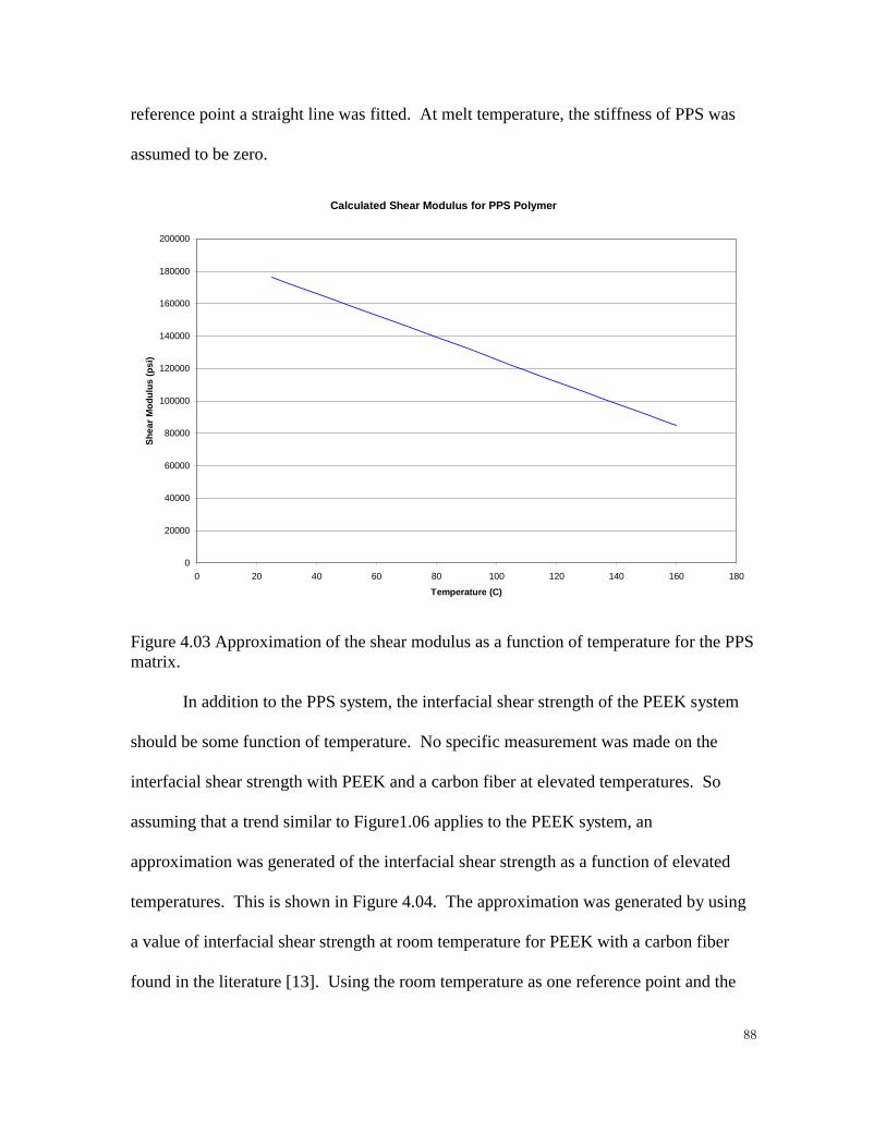
reference point a straight line was fitted. At melt temperature, the stiffness of PPS was

assumed to be zero.

Calculated Shear Modulus for PPS Polymer

0

20000

40000

60000

80000

100000

120000

140000

160000

180000

200000

0 20 40 60 80 100 120 140 160 180

Temperature (C)

Sh

ear

Mo

du

lus

(psi

)

Figure 4.03 Approximation of the shear modulus as a function of temperature for the PPSmatrix.

In addition to the PPS system, the interfacial shear strength of the PEEK system

should be some function of temperature. No specific measurement was made on the

interfacial shear strength with PEEK and a carbon fiber at elevated temperatures. So

assuming that a trend similar to Figure1.06 applies to the PEEK system, an

approximation was generated of the interfacial shear strength as a function of elevated

temperatures. This is shown in Figure 4.04. The approximation was generated by using

a value of interfacial shear strength at room temperature for PEEK with a carbon fiber

found in the literature [13]. Using the room temperature as one reference point and the

��

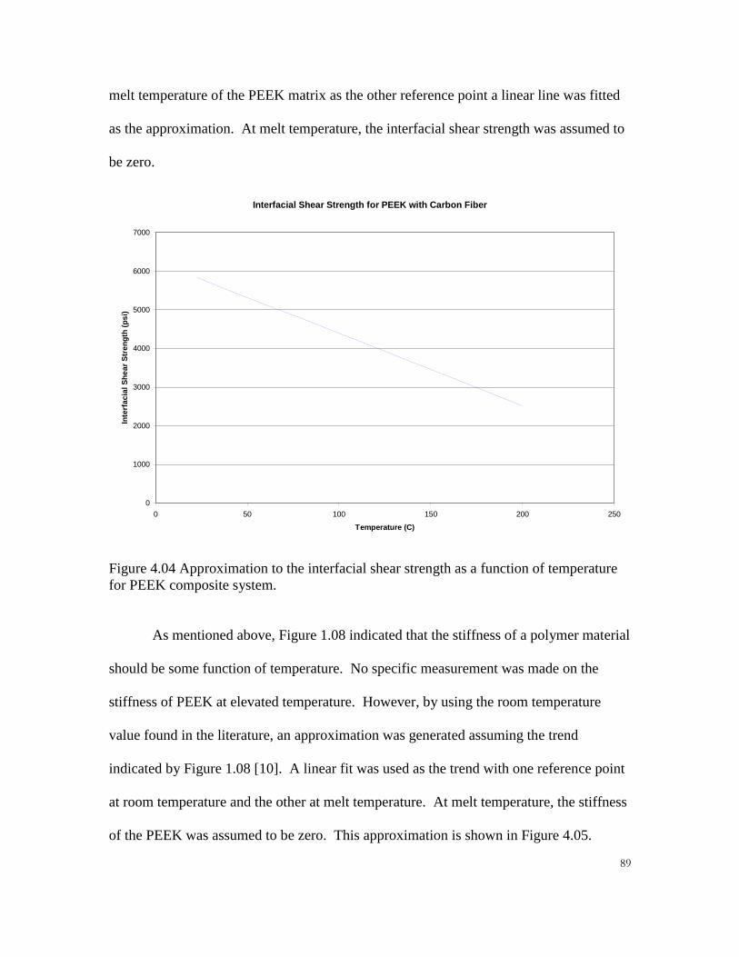
melt temperature of the PEEK matrix as the other reference point a linear line was fitted

as the approximation. At melt temperature, the interfacial shear strength was assumed to

be zero.

Interfacial Shear Strength for PEEK with Carbon Fiber

0

1000

2000

3000

4000

5000

6000

7000

0 50 100 150 200 250

Temperature (C)

Inte

rfac

ial S

hea

r S

tren

gth

(p

si)

Figure 4.04 Approximation to the interfacial shear strength as a function of temperaturefor PEEK composite system.

As mentioned above, Figure 1.08 indicated that the stiffness of a polymer material

should be some function of temperature. No specific measurement was made on the

stiffness of PEEK at elevated temperature. However, by using the room temperature

value found in the literature, an approximation was generated assuming the trend

indicated by Figure 1.08 [10]. A linear fit was used as the trend with one reference point

at room temperature and the other at melt temperature. At melt temperature, the stiffness

of the PEEK was assumed to be zero. This approximation is shown in Figure 4.05.

��

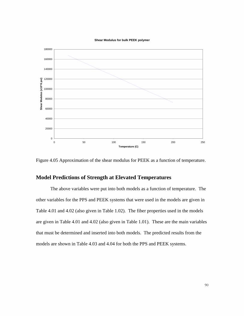
Shear Modulus for bulk PEEK polymer

0

20000

40000

60000

80000

100000

120000

140000

160000

180000

0 50 100 150 200 250

Temperature (C)

Sh

ear

Mo

du

lus

(x10

^6 p

si)

Figure 4.05 Approximation of the shear modulus for PEEK as a function of temperature.

Model Predictions of Strength at Elevated Temperatures

The above variables were put into both models as a function of temperature. The

other variables for the PPS and PEEK systems that were used in the models are given in

Table 4.01 and 4.02 (also given in Table 1.02). The fiber properties used in the models

are given in Table 4.01 and 4.02 (also given in Table 1.01). These are the main variables

that must be determined and inserted into both models. The predicted results from the

models are shown in Table 4.03 and 4.04 for both the PPS and PEEK systems.

��

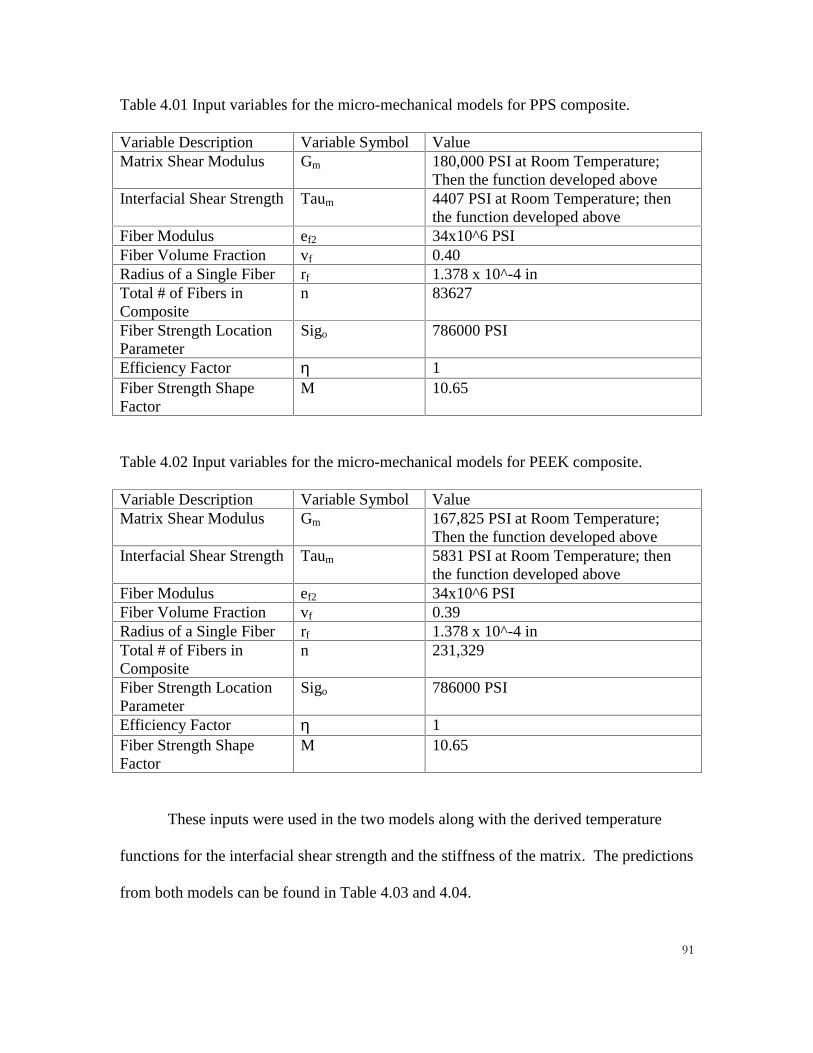
Table 4.01 Input variables for the micro-mechanical models for PPS composite.

Variable Description Variable Symbol ValueMatrix Shear Modulus Gm 180,000 PSI at Room Temperature;

Then the function developed aboveInterfacial Shear Strength Taum 4407 PSI at Room Temperature; then

the function developed aboveFiber Modulus ef2 34x10^6 PSIFiber Volume Fraction vf 0.40Radius of a Single Fiber rf 1.378 x 10^-4 inTotal # of Fibers inComposite

n 83627

Fiber Strength LocationParameter

Sigo 786000 PSI

Efficiency Factor η 1Fiber Strength ShapeFactor

M 10.65

Table 4.02 Input variables for the micro-mechanical models for PEEK composite.

Variable Description Variable Symbol ValueMatrix Shear Modulus Gm 167,825 PSI at Room Temperature;

Then the function developed aboveInterfacial Shear Strength Taum 5831 PSI at Room Temperature; then

the function developed aboveFiber Modulus ef2 34x10^6 PSIFiber Volume Fraction vf 0.39Radius of a Single Fiber rf 1.378 x 10^-4 inTotal # of Fibers inComposite

n 231,329

Fiber Strength LocationParameter

Sigo 786000 PSI

Efficiency Factor η 1Fiber Strength ShapeFactor

M 10.65

These inputs were used in the two models along with the derived temperature

functions for the interfacial shear strength and the stiffness of the matrix. The predictions

from both models can be found in Table 4.03 and 4.04.

��

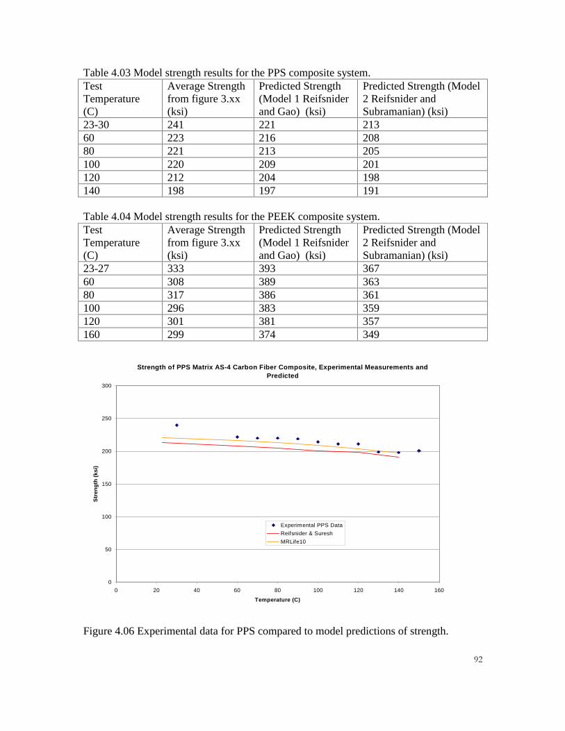
Table 4.03 Model strength results for the PPS composite system.TestTemperature(C)

Average Strengthfrom figure 3.xx(ksi)

Predicted Strength(Model 1 Reifsniderand Gao) (ksi)

Predicted Strength (Model2 Reifsnider andSubramanian) (ksi)

23-30 241 221 21360 223 216 20880 221 213 205100 220 209 201120 212 204 198140 198 197 191

Table 4.04 Model strength results for the PEEK composite system.TestTemperature(C)

Average Strengthfrom figure 3.xx(ksi)

Predicted Strength(Model 1 Reifsniderand Gao) (ksi)

Predicted Strength (Model2 Reifsnider andSubramanian) (ksi)

23-27 333 393 36760 308 389 36380 317 386 361100 296 383 359120 301 381 357160 299 374 349

Strength of PPS Matrix AS-4 Carbon Fiber Composite, Experimental Measurements and Predicted

0

50

100

150

200

250

300

0 20 40 60 80 100 120 140 160

Temperature (C)

Str

eng

th (

ksi)

Experimental PPS Data

Reifsnider & Suresh

MRLife10

Figure 4.06 Experimental data for PPS compared to model predictions of strength.

��

As shown in Figure 4.06, both models under-predict the average strength of the

PPS composite system. However, both of the models’ predictions are within the

experimental scatter of this system. Both models predict a 10 percent decrease in

strength from room temperature to 140 degrees Celsius. A R-squared linear fit for model

#2 gave a slope of -0.18 and a R-square value of 0.96. The same fit for model #1 gave a

slope of -0.19 and a R-square value of 0.96. The experimental results showed a 17

percent decrease in this temperature range for the PPS composite system. A R-squared

linear fit for the average experimental data gave a slope of 0.32 and a R-square value of

0.93. This difference could be a result of several factors. One such factor is that the

interfacial shear strength and the shear modulus assumptions in Figures 4.02 and 4.03 are

not accurate. More information must be determined to eliminate the guesswork for these

variables. Another factor could be due to the fact that the temperature is effecting more

variables than the interfacial shear strength and the matrix stiffness. Maybe the models

have not taken into account all the variables that control the strength.

��

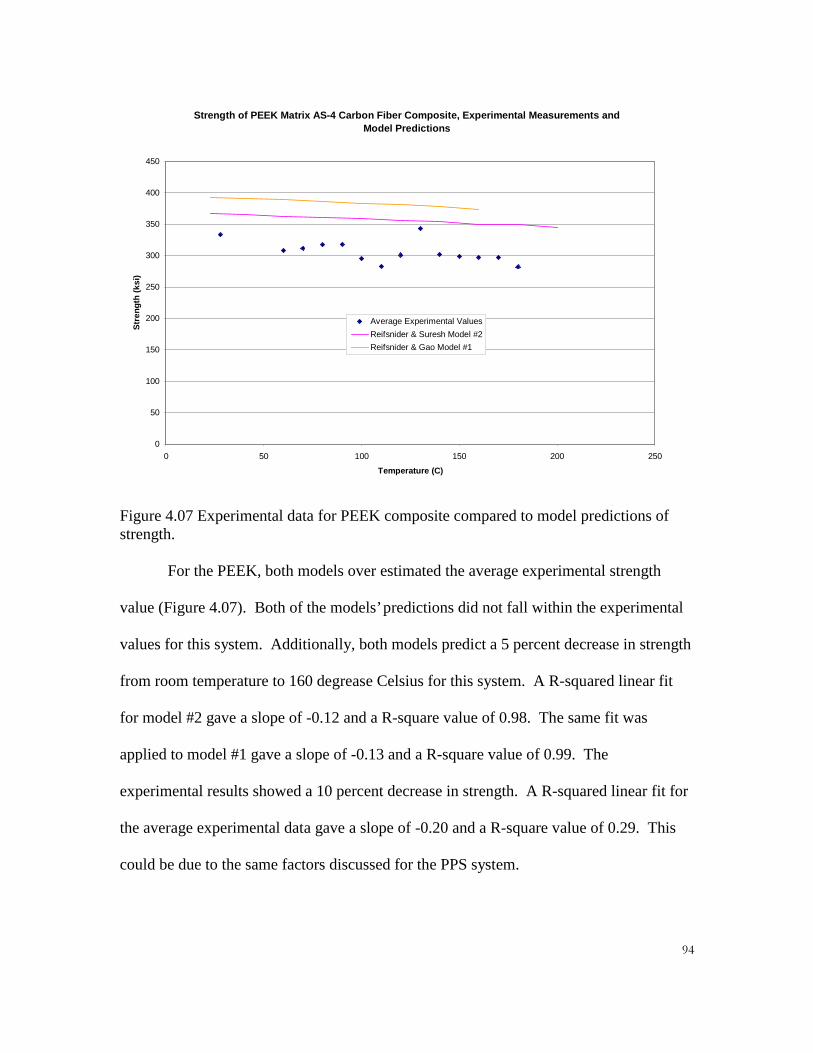
Strength of PEEK Matrix AS-4 Carbon Fiber Composite, Experimental Measurements and Model Predictions

0

50

100

150

200

250

300

350

400

450

0 50 100 150 200 250

Temperature (C)

Str

eng

th (

ksi)

Average Experimental Values

Reifsnider & Suresh Model #2

Reifsnider & Gao Model #1

Figure 4.07 Experimental data for PEEK composite compared to model predictions ofstrength.

For the PEEK, both models over estimated the average experimental strength

value (Figure 4.07). Both of the models’ predictions did not fall within the experimental

values for this system. Additionally, both models predict a 5 percent decrease in strength

from room temperature to 160 degrease Celsius for this system. A R-squared linear fit

for model #2 gave a slope of -0.12 and a R-square value of 0.98. The same fit was

applied to model #1 gave a slope of -0.13 and a R-square value of 0.99. The

experimental results showed a 10 percent decrease in strength. A R-squared linear fit for

the average experimental data gave a slope of -0.20 and a R-square value of 0.29. This

could be due to the same factors discussed for the PPS system.

��

V. Summary, Conclusions, and Future Work

Summary of Method

In order to predict the strength of a polymer composite in an environment of

elevated temperature, the temperature dependence of the two main variables must be

determined. These variables are the interfacial shear strength and the shear modulus of

the matrix material. If the information is not available then an approximation can be used

for these values. After these variables are determined, the micro-mechanical models can

be used to predict the temperature response of the composite system.

Conclusions

Based on these three systems, the strength of unidirectional polymer composite

systems can be expected to decrease with elevated temperatures between room

temperature and the glass transitional temperature. In addition to the strength the

stiffness of these systems can also be expected to decrease. The strength decrease can be

expected to be more than the stiffness decrease. For each of these materials, the

ineffective length is being increased as the temperature is elevated. This is concluded

because the matrix stiffness decreases. The change in the fracture mode of vinyl ester

also leads to this conclusion.

��

The vinyl ester system at the lower temperatures failed with more of the fibers

grouped together. At the higher temperatures, the fracture was less clumped with groups

of fibers and consisted more of single fibers. In this case, ineffective lengths were larger

and fiber fracture regions interacted more readily to cause failure.

Based on recent research efforts, the interfacial shear strength of a polymer matrix

and a carbon fiber can be expected to decrease with elevated temperatures. The

interfacial strength and stiffness also controls the ineffective length. In addition to the

interfacial shear strength, the stiffness of a polymer can be expected to decrease with

elevated temperatures. The combination of these effects can be placed in micro-

mechanical models to give a reasonable prediction. Therefore, this method is a viable for

predicting the failure strength of unidirectional polymer carbon fiber composite systems.

Future Work

More work should be done on the interfacial shear strengths as a function of

temperature. The accuracy of this parameter can make models more accurate in their

predictions. In addition, the stiffness as a function of temperature of PPS and PEEK must

be more accurately determined. These variables should also be explored for cryogenic

temperatures.

The study involved the response of strength in the tensile fiber direction.

Additional information of the effect of elevated temperatures should be explored for off-

axis (+45/-45) orientations. This type of test would produce the macro-mechanical shear

modulus of the composite as a function of temperature. It also will produce a shear

strength of the composite as a function of temperature. A panel of the same PEEK (AS-

��

4) in this study has been produced with this lay-up. The lay-up of this panel is a

symmetric sixteen-ply +45/-45 orientation. CEA-06-125UW-350 strain gages have been

placed on the specimens with M-Bond 600.

This same method should apply to the cryogenic temperatures. More data should

be obtained at these temperatures. The chamber for this environment should be further

advanced and better controlled. At cryogenic temperatures, the ineffective length should

be small and this will cause higher stress concentrations.

An additional material should be investigated for its response at elevated

temperatures. This material should be an epoxy system with carbon fibers (AS-4). This

system is ideal to test this method due to the fact that the interfacial shear strength is

given for this particular system as a function of temperature (Figure 1.06). In addition to

the known interfacial shear strength, the stiffness of this material is known as a function

of temperature. For this study, two different panels have been produced with different

cure cycles. These different processes are given in Figures 5.01 and 5.02. The material

was donated by Adhesive Prepregs for Composites Manufacturers. It is identified by the

name DA 4518U and is a toughened modified epoxy resin system. This material was

processed in the platen hot press with a lay-up of seven-ply unidirectional fiber

orientation.

��

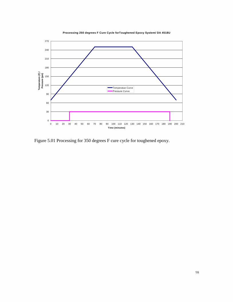
Processing 250 degrees F Cure Cycle forToughened Epoxy System/ DA 4518U

0

30

60

90

120

150

180

210

240

270

0 10 20 30 40 50 60 70 80 90 100 110 120 130 140 150 160 170 180 190 200 210

Time (minutes)

Tem

per

atu

re (

F)

/ P

ress

ure

(p

si)

Temperatue Curve

Pressure Curve

Figure 5.01 Processing for 350 degrees F cure cycle for toughened epoxy.

��

Processing 350 degrees F Cure Cycle For Toughened Epoxy/ DA 4518U

0

25

50

75

100

125

150

175

200

225

250

275

300

325

350

375

0 20 40 60 80 100 120 140 160 180 200 220 240 260 280 300

Time (minutes)

Tem

per

atu

re(F

)/P

ress

ure

(Psi

)

Temperature Curve

Pressure Curve

Figure 5.02 Processing for 250 degrees F cure cycle for toughened epoxy.

���

REFERENCES:

1. Subramanian, S., Reifsnider, K.L., and Stinchcomb, W.W., “Tensile Strength ofUnidirection Composites: The Role of Efficiency and Strength of Fiber-MatrixInterface,” Journal of Composites Technology & Research, JCTRER, Vol.17,No.4, October 1995, pp. 239-300.

2. MRLife10, "A Strength and Life Prediction Code for Laminated CompositeMaterials," S. Case and K.L. Reifsnider, Materials Response Group, VirginiaPolytechnic Institute and State University, 1997.

3. Gao, Z., and Reifsnider, K.L., “Micromechanics of Tensile Strength in CompositeSystems,” Composite Materials: Fatigue and Fracture, Fourth Volume, ASTMSTP 1156, W.W. Stinchcomb and N.E. Ashbaugh, Eds., American Society forTesting and Materials, Philadelphia, 1993, pp. 453-470.

4. Reifsnider K.L., ESM 6104 Class Notes, Department of Engineering Science andMechanics, Virginia Polytechnic Institute & State University.

5. Reifsnider, K.L., Case, Scott, “Mechanics of Temperature-Driven Long-TermEnvironmental Degradation of Polymer-Based Composite Systems,” Departmentof Engineering Science and Mechanics, Virginia Polytechnic Institute and StateUniversity, Blacksburg, Virginia.

6. NASA Contractor Report # 178272, "Time-Temperature-Stress Capabilities ofComposite Materials for Advanced Supersonic Technology Application," J.R.Kerr and J.F. Haskins, NASA, May 1987.

7. H. Zhuang and J.P. Wightman, "The Influence of Surface Properties on CarbonFiber / Epoxy Matrix Interfacial Adhesion," Journal of Adhesion, 1996, Vol. 62,pp. 213-245.

8. A.S. Wimolkiatisak and J. P. Bell, "Interfacial Shear Strength and Failure Modesof Interphase-Modified Graphite-Epoxy Composites," Polymer Composites, June1989, Vol. 10, No.3, pp. 162-172.

9. Charles A. Harper, "Handbook of Plastics, Elastomers, and Composites," ThirdEdition, McGraw-Hill Companies, Inc., 1996.

10. P.K. Mallick, "Fiber-Reinforced Composites," Second Edition, Marcel Dekker,Inc., 1993.

���

11. A.J. Kinloch, "Adhesion and Adhesives," Chapman & Hall, London, 1987

12. ASTM Designation D 3039/D 3039M - 93, "Standard Test Method for TensileProperties of Polymer Matrix Composite Materials," 1993

13. S. L. Chuang and Ning-Jo Chu, "Effect of Polyamic Acids on Interfacial ShearStrength in Carbon Fiber / Aromatic Thermoplastics," Journal of Applied PolymerScience, Vol. 41, 1990, pp. 373-382.

���

APPENDIX A: PPS RAW DATA

���

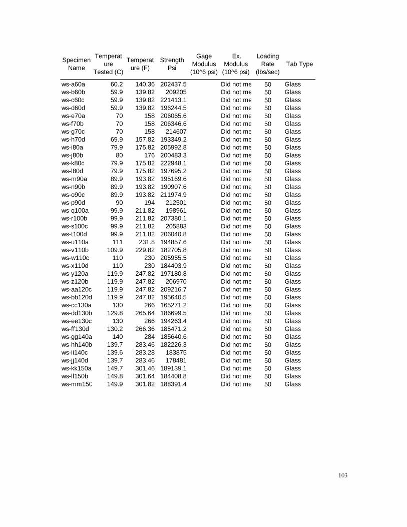
Specimen Name

Temperature

Tested (C)

Temperature (F)

Strength Psi

Gage Modulus

(10^6 psi)

Ex. Modulus

(10^6 psi)

Loading Rate

(lbs/sec)Tab Type

ws-a60a 60.2 140.36 202437.5 Did not me 50 Glassws-b60b 59.9 139.82 209205 Did not me 50 Glassws-c60c 59.9 139.82 221413.1 Did not me 50 Glassws-d60d 59.9 139.82 196244.5 Did not me 50 Glassws-e70a 70 158 206065.6 Did not me 50 Glassws-f70b 70 158 206346.6 Did not me 50 Glassws-g70c 70 158 214607 Did not me 50 Glassws-h70d 69.9 157.82 193349.2 Did not me 50 Glassws-i80a 79.9 175.82 205992.8 Did not me 50 Glassws-j80b 80 176 200483.3 Did not me 50 Glassws-k80c 79.9 175.82 222948.1 Did not me 50 Glassws-l80d 79.9 175.82 197695.2 Did not me 50 Glassws-m90a 89.9 193.82 195169.6 Did not me 50 Glassws-n90b 89.9 193.82 190907.6 Did not me 50 Glassws-o90c 89.9 193.82 211974.9 Did not me 50 Glassws-p90d 90 194 212501 Did not me 50 Glassws-q100a 99.9 211.82 198961 Did not me 50 Glassws-r100b 99.9 211.82 207380.1 Did not me 50 Glassws-s100c 99.9 211.82 205883 Did not me 50 Glassws-t100d 99.9 211.82 206040.8 Did not me 50 Glassws-u110a 111 231.8 194857.6 Did not me 50 Glassws-v110b 109.9 229.82 182705.8 Did not me 50 Glassws-w110c 110 230 205955.5 Did not me 50 Glassws-x110d 110 230 184403.9 Did not me 50 Glassws-y120a 119.9 247.82 197180.8 Did not me 50 Glassws-z120b 119.9 247.82 206970 Did not me 50 Glassws-aa120c 119.9 247.82 209216.7 Did not me 50 Glassws-bb120d 119.9 247.82 195640.5 Did not me 50 Glassws-cc130a 130 266 165271.2 Did not me 50 Glassws-dd130b 129.8 265.64 186699.5 Did not me 50 Glassws-ee130c 130 266 194263.4 Did not me 50 Glassws-ff130d 130.2 266.36 185471.2 Did not me 50 Glassws-gg140a 140 284 185640.6 Did not me 50 Glassws-hh140b 139.7 283.46 182226.3 Did not me 50 Glassws-ii140c 139.6 283.28 183875 Did not me 50 Glassws-jj140d 139.7 283.46 178481 Did not me 50 Glassws-kk150a 149.7 301.46 189139.1 Did not me 50 Glassws-ll150b 149.8 301.64 184408.8 Did not me 50 Glassws-mm150 149.9 301.82 188391.4 Did not me 50 Glass

���

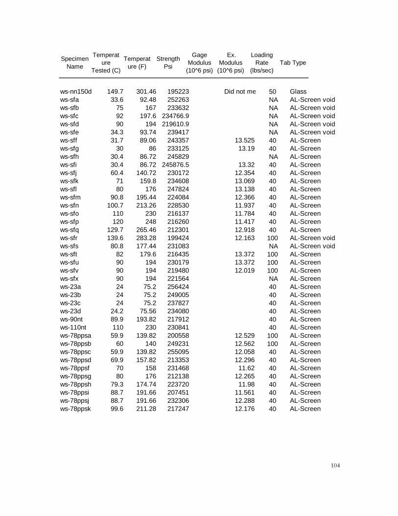
Specimen Name

Temperature

Tested (C)

Temperature (F)

Strength Psi

Gage Modulus

(10^6 psi)

Ex. Modulus

(10^6 psi)

Loading Rate

(lbs/sec)Tab Type

ws-nn150d 149.7 301.46 195223 Did not me 50 Glassws-sfa 33.6 92.48 252263 NA AL-Screen voidws-sfb 75 167 233632 NA AL-Screen voidws-sfc 92 197.6 234766.9 NA AL-Screen voidws-sfd 90 194 219610.9 NA AL-Screen voidws-sfe 34.3 93.74 239417 NA AL-Screen voidws-sff 31.7 89.06 243357 13.525 40 AL-Screenws-sfg 30 86 233125 13.19 40 AL-Screenws-sfh 30.4 86.72 245829 NA AL-Screenws-sfi 30.4 86.72 245876.5 13.32 40 AL-Screenws-sfj 60.4 140.72 230172 12.354 40 AL-Screenws-sfk 71 159.8 234608 13.069 40 AL-Screenws-sfl 80 176 247824 13.138 40 AL-Screenws-sfm 90.8 195.44 224084 12.366 40 AL-Screenws-sfn 100.7 213.26 228530 11.937 40 AL-Screenws-sfo 110 230 216137 11.784 40 AL-Screenws-sfp 120 248 216260 11.417 40 AL-Screenws-sfq 129.7 265.46 212301 12.918 40 AL-Screenws-sfr 139.6 283.28 199424 12.163 100 AL-Screen voidws-sfs 80.8 177.44 231083 NA AL-Screen voidws-sft 82 179.6 216435 13.372 100 AL-Screenws-sfu 90 194 230179 13.372 100 AL-Screenws-sfv 90 194 219480 12.019 100 AL-Screenws-sfx 90 194 221564 NA AL-Screenws-23a 24 75.2 256424 40 AL-Screenws-23b 24 75.2 249005 40 AL-Screenws-23c 24 75.2 237827 40 AL-Screenws-23d 24.2 75.56 234080 40 AL-Screenws-90nt 89.9 193.82 217912 40 AL-Screenws-110nt 110 230 230841 40 AL-Screenws-78ppsa 59.9 139.82 200558 12.529 100 AL-Screenws-78ppsb 60 140 249231 12.562 100 AL-Screenws-78ppsc 59.9 139.82 255095 12.058 40 AL-Screenws-78ppsd 69.9 157.82 213353 12.296 40 AL-Screenws-78ppsf 70 158 231468 11.62 40 AL-Screenws-78ppsg 80 176 212138 12.265 40 AL-Screenws-78ppsh 79.3 174.74 223720 11.98 40 AL-Screenws-78ppsi 88.7 191.66 207451 11.561 40 AL-Screenws-78ppsj 88.7 191.66 232306 12.288 40 AL-Screenws-78ppsk 99.6 211.28 217247 12.176 40 AL-Screen

���

Specimen Name

Temperature

Tested (C)

Temperature (F)

Strength Psi

Gage Modulus

(10^6 psi)

Ex. Modulus

(10^6 psi)

Loading Rate

(lbs/sec)Tab Type

ws-78ppsl 98.6 209.48 217673 11.959 40 AL-Screenws-78ppsm 108.6 227.48 216316 n/a 40 AL-Screenws-78ppsn 109 228.2 224554 12.067 40 AL-Screenws-78ppso 119.6 247.28 234583 12.112 40 AL-Screenws-78ppsp 119.6 247.28 200936 12.401 40 AL-Screenws-78ppsq 128.6 263.48 211534 11.862 40 AL-Screenws-78ppsr 129.2 264.56 210438 12.165 40 AL-Screenws-78ppss 139.1 282.38 208816 12.126 40 AL-Screenws-78ppst 139.2 282.56 196695 12.832 40 AL-Screenws-718a 69.9 157.82 232685 11.954 100 Glassws-718b 79.7 175.46 219568 12.342 100 Glassws-718c 90 194 235871 12.383 100 Glassws-718d 99.4 210.92 224690 12.605 40 Glassws-718e 109.7 229.46 220594 12.394 40 Glassws-718f 119.8 247.64 215739 11.844 40 Glassws-718g 129.2 264.56 216234 10.288 40 Glassws-718h 139.1 282.38 221262 n/a 40 Glassws-718i 149.5 301.1 207845 12.301 40 Glassws-718j 32.5 90.5 240505 12.192 40 Glassws-78ppsv 149.2 300.56 210904 13.917 40 AL-Screenws-78ppsx 149.1 300.38 222977 13.577 40 AL-Screenws-81a 31.1 87.98 221697 12.053 150 AL-Screenws-81b 31.1 87.98 235144 12.12 150 AL-Screenws-81c 31.1 87.98 239167 11.73 150 AL-Screenws-81d 31.1 87.98 243687 12.62 150 AL-Screenws-81e 59.9 139.82 225760 12.206 150 AL-Screenws-81f 59.9 139.82 235443 12.357 150 AL-Screenws-81g 59.9 139.82 233709 11.918 150 AL-Screenws-81h 59.9 139.82 213313 12.253 150 AL-Screenws-81i 69.5 157.1 217467 12.358 150 AL-Screenws-81j 69.6 157.28 227339 12.214 150 AL-Screenws-81k 69.6 157.28 236750 13.893 150 AL-Screenws-81l 69.5 157.1 230590 11.89 150 AL-Screenws-81m 79.4 174.92 225825 12.023 150 AL-Screenws-81n 79.4 174.92 224869 12.87 150 AL-Screenws-81o 79.7 175.46 238901 11.181 150 AL-Screenws-81p 79.9 175.82 225000 11.789 150 AL-Screenws-81q 89.5 193.1 237083 12.772 150 AL-Screenws-81r 89.2 192.56 237164 12.116 150 AL-Screenws-81s 89.4 192.92 220410 11.997 150 AL-Screen

���

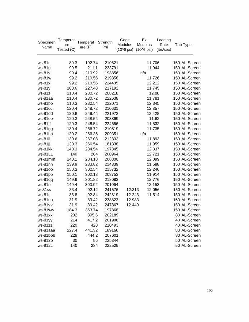
Specimen Name

Temperature

Tested (C)

Temperature (F)

Strength Psi

Gage Modulus

(10^6 psi)

Ex. Modulus

(10^6 psi)

Loading Rate

(lbs/sec)Tab Type

ws-81t 89.3 192.74 210621 11.706 150 AL-Screenws-81u 99.5 211.1 233791 11.944 150 AL-Screenws-81v 99.4 210.92 193856 n/a 150 AL-Screenws-81w 99.2 210.56 219858 11.726 150 AL-Screenws-81x 99.2 210.56 224435 12.212 150 AL-Screenws-81y 108.6 227.48 217192 11.745 150 AL-Screenws-81z 110.4 230.72 208218 12.08 150 AL-Screenws-81aa 110.4 230.72 222638 11.781 150 AL-Screenws-81bb 110.3 230.54 222071 12.345 150 AL-Screenws-81cc 120.4 248.72 210631 12.357 150 AL-Screenws-81dd 120.8 249.44 221972 12.428 150 AL-Screenws-81ee 120.3 248.54 203869 11.62 150 AL-Screenws-81ff 120.3 248.54 224656 11.832 150 AL-Screenws-81gg 130.4 266.72 210819 11.735 150 AL-Screenws-81hh 130.2 266.36 209351 n/a 150 AL-Screenws-81ii 130.6 267.08 212332 11.893 150 AL-Screenws-81jj 130.3 266.54 181338 11.959 150 AL-Screenws-81kk 140.3 284.54 197345 12.337 150 AL-Screenws-81LL 140 284 200964 12.721 150 AL-Screenws-81mm 140.1 284.18 208300 12.099 150 AL-Screenws-81nn 139.9 283.82 214339 11.588 150 AL-Screenws-81oo 150.3 302.54 215732 12.246 150 AL-Screenws-81pp 150.1 302.18 208753 11.914 150 AL-Screenws-81qq 149.9 301.82 218083 12.776 150 AL-Screenws-81rr 149.4 300.92 201064 12.153 150 AL-Screenws81ss 33.4 92.12 241576 12.313 12.056 150 AL-Screenws-81tt 33.8 92.84 242819 12.243 11.514 150 AL-Screenws-81uu 31.9 89.42 238823 12.983 150 AL-Screenws-81vv 31.9 89.42 247867 12.449 150 AL-Screenws-81ww 184.3 363.74 197868 150 AL-Screenws-81xx 202 395.6 202189 80 AL-Screenws-81yy 214 417.2 201908 40 AL-Screenws-81zz 220 428 210493 40 AL-Screenws-81aaa 227.4 441.32 189166 80 AL-Screenws-81bbb 229 444.2 207601 80 AL-Screenws-912b 30 86 225344 50 AL-Screenws-912c 140 284 222529 50 AL-Screen

���

Specimen Name

Temperature

Tested (C)

Temperature (F)

Strength Psi

Gage Modulus

(10^6 psi)

Ex. Modulus

(10^6 psi)

Loading Rate

(lbs/sec)Tab Type

ws-912d 159.9 319.82 212621 50 AL-Screenws-912e 119.5 247.1 213968 11.767 50 AL-Screenws-912f 99.5 211.1 219003 11.919 50 AL-Screenws-912g 150.3 302.54 220627 50 AL-Screenws-912h 89.8 193.64 230160 12.491 50 AL-Screenws-912k 159.9 319.82 211474 50 AL-Screenws-912l 109.6 229.28 219153 12.216 50 AL-Screenws-912m 129.2 264.56 224527 12.773 50 AL-Screenws-912n 80 176 235518 12.597 50 AL-Screenws-912o 60 140 12.528 50 AL-Screenws-912p 69.9 157.82 222953 11.826 50 AL-Screenws-cl1 -142.7 -225 176000 NA 100 AL-Screenws-cl2 -184 -300 240700 NA 50 AL-Screenws-cl3 -184 -300 266000 NA 50 AL-Screen

���

APPENDIX B: PEEK RAW DATA

���

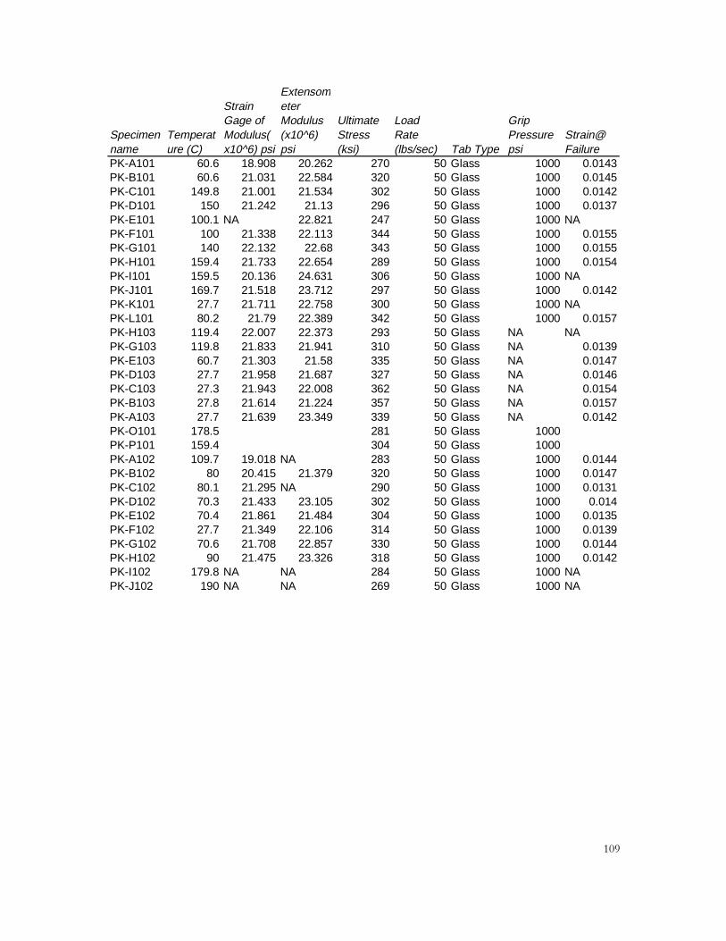
Specimen name

Temperature (C)

Strain Gage of Modulus(x10^6) psi

Extensometer Modulus (x10^6) psi

Ultimate Stress (ksi)

Load Rate (lbs/sec) Tab Type

Grip Pressure psi

Strain@ Failure

PK-A101 60.6 18.908 20.262 270 50 Glass 1000 0.0143PK-B101 60.6 21.031 22.584 320 50 Glass 1000 0.0145PK-C101 149.8 21.001 21.534 302 50 Glass 1000 0.0142PK-D101 150 21.242 21.13 296 50 Glass 1000 0.0137PK-E101 100.1 NA 22.821 247 50 Glass 1000 NAPK-F101 100 21.338 22.113 344 50 Glass 1000 0.0155PK-G101 140 22.132 22.68 343 50 Glass 1000 0.0155PK-H101 159.4 21.733 22.654 289 50 Glass 1000 0.0154PK-I101 159.5 20.136 24.631 306 50 Glass 1000 NAPK-J101 169.7 21.518 23.712 297 50 Glass 1000 0.0142PK-K101 27.7 21.711 22.758 300 50 Glass 1000 NAPK-L101 80.2 21.79 22.389 342 50 Glass 1000 0.0157PK-H103 119.4 22.007 22.373 293 50 Glass NA NAPK-G103 119.8 21.833 21.941 310 50 Glass NA 0.0139PK-E103 60.7 21.303 21.58 335 50 Glass NA 0.0147PK-D103 27.7 21.958 21.687 327 50 Glass NA 0.0146PK-C103 27.3 21.943 22.008 362 50 Glass NA 0.0154PK-B103 27.8 21.614 21.224 357 50 Glass NA 0.0157PK-A103 27.7 21.639 23.349 339 50 Glass NA 0.0142PK-O101 178.5 281 50 Glass 1000PK-P101 159.4 304 50 Glass 1000PK-A102 109.7 19.018 NA 283 50 Glass 1000 0.0144PK-B102 80 20.415 21.379 320 50 Glass 1000 0.0147PK-C102 80.1 21.295 NA 290 50 Glass 1000 0.0131PK-D102 70.3 21.433 23.105 302 50 Glass 1000 0.014PK-E102 70.4 21.861 21.484 304 50 Glass 1000 0.0135PK-F102 27.7 21.349 22.106 314 50 Glass 1000 0.0139PK-G102 70.6 21.708 22.857 330 50 Glass 1000 0.0144PK-H102 90 21.475 23.326 318 50 Glass 1000 0.0142PK-I102 179.8 NA NA 284 50 Glass 1000 NAPK-J102 190 NA NA 269 50 Glass 1000 NA

���

APPENDIX C: VINYL ESTER RAW DATA

���

Specimenname

Temperature (C)

UltimateStress(psi)

Load Rate(lbs/sec)

Modulus(x10^6)psi

Tab Type

ve-zteca 70 107663 100 14.659 Al-Wireve-ztecb 90 104445 100 14.956 Al-Wireve-ztecc 110 88302 100 14.669 Al-Wireve-ztecd 130 83556 100 14.558 Al-Wireve-ztece 140 76157 100 14.618 Al-Wireve-ztecf 35 118092 100 16.23 Al-Wireve-ztech 90 99144 100 15.826 Al-Wireve-zteci 110 89696 100 14.11 Al-Wireve-ztecm -123.3 131522 100 NA Al-Wireve-ztecl 69.8 104961 40 NA Al-Wireve-ztecj 32.2 100977 40 NA Al-Wireve-puc 90 124828 100 17.052 Al-Wireve-pud 109.3 129861 100 16.773 Al-Wireve-pue 129.7 121691 100 16.303 Al-Wireve-puf 149.7 108788 100 NA Al-Wireve-pug -101 155987 100 17.695 Al-Wireve-pui -184.4 165400 100 18.109 Al-Wireve-puj -184.4 180600 100 18.68 Al-Wireve-puk -184.4 180800 100 19.4 Al-Wireve-pua 33.4 161167 100 17.7 Al-Wireve-pub 34 159591 100 18.4 Al-Wire

���

VITA

Brady M. Walther was born on August 17, 1971 to Jane and Phillip M. Walther in

Columbus, OH. After eighteen years in Gahanna Ohio, he graduated from Gahanna

Lincoln High School in spring of 1990. Brady then went to Emory & Henry College in

Emory Virginia in the fall of 1990. He also enrolled at the University of Tennessee at

Knoxville in the fall of 1992. Mr. Walther graduated with Bachelor of Science degree

from institutions in spring 1996. He majored in Physics, Mathematics, and Engineering

Science and Mechanics. In the fall of 1996, Brady enrolled in the Graduate School of

Virginia Polytechnic Institute and State University under the program of Engineering

Mechanics. In the summer of 1998, Mr. Walther graduated with a Master of Science

degree.