an investment strategy based on stochastic unit root models - copy

International Journal of Economics and Finance; Vol. 5, No. 3; 2013 ISSN 1916-971X E-ISSN 1916-9728

Published by Canadian Center of Science and Education

221

An Investment Strategy Based on Stochastic Unit Root Models

Mamadou A. Konté1

1 Université Gaston Berger, UFR Sciences Economiques et de Gestion, BP 234 Saint Louis, Sénégal

Correspondence: Mamadou A. Konté, Université Gaston Berger, UFR Sciences Economiques et de Gestion, BP 234 Saint Louis, Sénégal. Tel: 221-77-622-1350. E-mail: [email protected] or [email protected]

Received: September 29, 2012 Accepted: January 17, 2013 Online Published: February 26, 2013

doi:10.5539/ijef.v5n3p221 URL: http://dx.doi.org/10.5539/ijef.v5n3p221

Abstract

An algorithm is presented that locally approximates the nonlinearity of stochastic unit root (STUR) models by n linear models. The previous integer n is chosen so that the Hadamard matrix of order n can be defined. The strategy STUR(n), then consists in creating n linear models from this Hadamard matrix and taking their average forecast. A purchase (sell) signal is made if the obtained average forecast is positive (negative). Subsequently, a comparison is made with respect to competing models (Moving average strategies) to assess their ability to forecast the variation of five international indexes. It is found, after taking account transaction costs, that STUR(n) generates generally the highest profitability in the out-of-sample data.

Keywords: forecasting, trading rules, random coefficient autoregressive models, efficiency market hypothesis

1. Introduction

The question of Efficiency Market Hypothesis (EMH) has been studied for many years by both academics and market participants. The aim is to see if the assumptions of market frictionless and traders rationality are a good description of real markets where microstructure (transaction costs, information asymmetry, etc.) and noise traders are present. This is an ongoing debate and there has been no consensus. That is why some authors have tried to reconcile the EMH and Behavioral finance arguments through dynamic systems, see for example Lo (2005) and Konté (2010). The empirical studies of this hypothesis are based generally on three classes. The first is traditional regression models. Their aim is to test the validity of the EMH in its weak form through traditional time series forecast such as Auto Regressive Moving average models ARMA(p,q). If the market is supposed to be a nonlinear dynamic system, one may consider nonlinear models such as the Random Coefficient Autoregressive RCA(p) or regime switching models among others. The traditional regression models also contain analysis tools based on firms’ fundamental (dividend, Book-to-Market, etc.). In this case, the objective is to test the EMH in its semi-strong form (fundamental analysis). We refer to Ou and Penman (1989) and references therein.

The second class uses Technical Analysis tools such as Moving Average, Support and Resistance methods. This approach is widely applied by traders to detect trends or reversal effects by using information such that prices, trading volume, etc. Here, the validity of EMH is tested through its weak form, see for example Sullivan et al., (1999).

The last class, based on Machine Learning (Genetic Algorithms, Neural Networks methods) investigates the EMH in its weak and semi-strong form as for the class of traditional regression models. Their difference is that Machine learning models are self-adaptive methods in that there are few a priori assumptions about the relationship between inputs while the traditional regression models make strong assumptions (parametric approach).

The paper belongs to the first class where the nonlinearity of financial asset prices is modeled by RCA(p). This econometric model generates the main stylized facts of financial time series, see Yoon (2003). It may be also related to an Agent Based Model with a switching phenomenon between fundamentalists and noise traders, see for example Konté (2011). There are many methods proposed in the literature to estimate its parameters for trading or forecast purpose. For example Nicholls and Quinn (1981) employed the traditional least squares and the maximum likelihood methods, see also Granger and Swanson (1997). Wang and Ghosh (2002) use Bayesian approach while Sollis et al. (2000) work with Kalman filter. We follow here another approach consisting to approximate the RCA(1) model by n simple linear models where n is any integer such that the Hadamard matrix

www.ccsenet.org/ijef International Journal of Economics and Finance Vol. 5, No. 3; 2013

222

H of order n can be defined. The latter is an n × n matrix with all its elements being either −1 or 1, and such that

HHT=n*In where HT is the transpose of H, In is the identity matrix of order n. Therefore, the Hadamard

matrix columns is an orthogonal binary basis of Rn explaining why it is widely used in physics particularly in the field of signal transmission. The integer n, in this study, must satisfy the constraint n , n/12 or n/20 is a power of 2. The prediction is then made by taking the average forecast of these n linear models extracted from the Hadamatrix since many researchers agree that combining multiple forecasts leads to increased accuracy, see Granger and Ramanathan (1984).

The paper contributes in two ways to the literature. First, contrarily to other forecasting methods, the estimation procedure is made locally to capture traders’ feedback or interaction since the variance and other higher moments of STUR model do not exist. Only n data are used in the linear regression models where 8≤n≤50. This constraint gives us exactly height (08) strategies STUR(n) with n∈{8, 12, 16, 20, 24, 32, 40, 48}. The second contribution shows an application of the Hadamard basis to reduce the complexity of a problem (from exponential to linear) for trading purposes.

The paper is divided into four additional sections. Section 2 presents our methodology and its competing strategies to forecast the variation of asset prices of five international indexes (CAC 40, DAX 30, FTSE 100, Nikkei 225, S&P 500). Section 3 describes the data and the methodology used in the empirical application. Section 4 presents the empirical results and the last section concludes.

2. Some Forecasting Rules

2.1 Our Methodology

Consider the following stochastic unit root STUR(1) model defined by:

tttt yby 1)1( (1)

0),cov(,)(,)(,0)()( 2222 tttttt bEbEEbE

where (εt) is an i.i.d Gaussian process and yt=logSt (log of asset prices).

The properties of eq. (1), to replicate financial times series, have been studied by (Yoon, 2003). The econometric model is also related to an agent based model with interaction between fundamentalist and noise traders, see (Konté, 2011). It is a special case of the Random Coefficient Autoregressive RCA(1) model which is defined by:

yt = (φ+bt)yt−1 + εt

.),cov(,)(,)(,0)()( 2222 tttttt bEbEEbE

(Nicholls and Quinn, 1982) have shown that the RCA(1) process (yt) is a finite second-order stationary moment

if the condition φ2+ω2<1 is satisfied. Since φ=1 in our case, the stationary condition is violated (Note 1). That means conventional methods based on this assumption such as Maximum likelihood method cannot perform, see Yoon (2006) (Note 2). Consequently, we propose a methodology that locally approximates the nonlinearity of asset prices by n linear models. For this purpose, bt is supposed to take only two values α and −α at any time.

Therefore, it may be rewritten as bt=αXt−1 where for any t, Xt−1=1 or Xt−1=−1. The equation (1) becomes

tttttttt yXcyySSr 1111loglog (2)

where a constant c is added, as usual, in the regression model.

For the moment, the estimation cannot be proceed because the variable Xt−1 is not known. To circumvent this

problem, regressions models are used conditional on the path of (Xt). For example, in the equation (2), if it is

decided to use n data for the estimation process, we will have 2n paths for (Xt) , t=1,⋯,n since Xt takes −1 or

1 at any time. Each trajectory generates a linear model with three input variables Xt−1, yt−1 and the constant

variable c. Therefore, the nonlinearity is approximated by 2n linear models (Note 3). This feature comes at a

cost, as we need to store a binary matrix of size n×2n−1 to make all linear regressions (Note 4). Generally, we need the parameter n to be big for estimation precisions but not too much to keep a local approximation. In the application, it is taken 8≤n≤50. To solve the dimensionality problem, techniques similar to Component Principal


223

Analysis (CPA) in exploratory data analysis are used. Namely, we extract "n orthogonal linear models". Here,

the orthogonality of two models i and j is defined by the orthogonality of their corresponding paths (Xit−k) and

(Xjt−k), k=1,⋯,n. If n is constrained to be an integer such that n/2, n/12 or n/20 is equal to 2k, k∈N, then

Hadamard matrices exist. For example for n=2, the Hadamard matrix is

11

112H

that is a basis of R2. Recursively, we can define the matrix H4, H8, ⋯, by using the following formula

nn

nnn HH

HHH 2

This approach allows to pass from exponential (2n) to linear (n) complexity since now for n data used in the equation (2), n linear models are also employed where their paths correspond to the columns of the Hadamard matrix of order n. For each model, determined by the path of (Xt), the parameters α and c are estimated by the

Ordinary Least Square method. Then a forecast is made at time t+1 through the equation

ttttt yXcyyr ̂ˆˆˆ 11 (3)

A recursive regression is applied. At any time, the previous n data are used in the regression model to determine the new estimated parameters. We denote by )(nSUR the strategy that consists to take the average

forecasts of all n "orthogonal linear models". The procedure to create the buy and sell signals is then simple: a

buy (sell) signal is produced if the average forecast, denoted by 1ˆ tar , is positive (negative). To reduce the

number of transaction costs, we enhance the strategy by allowing static positions in the case where the forecast signal is not significant. In other words, the following strategy is applied for )(nSUR .

.),1(

30/))min()(max(;|)ˆ|)ˆ(

),(

11

otherwisentposition

RRccarifarsign

ntposition

tttt

where Rt=logSt−logSt−1 represents the index return at time t (Note 6). The sign function is defined by

sign(x)=1 if x>0, sign(x)=−1 if x<0 and sign(0)=0.

2.2 Competing Trading Rules

If the market is supposed to be efficient, an optimal strategy is to buy and hold an index. The strategy B&H consists therefore to be long on the index at any time and consequently there are no transaction costs. We consider also simple and exponential moving average strategies that have been widely used by traders to capt momentums or reversal effects. The idea is to consider two moving average series M(n,t) and M(m,t) with different lengths n and m. If we denote by (St) the asset price process, the simple and exponential moving

average are defined, for a given length k>0, by respectively the equations (4) and (5).

it

k

i

Sk

tkM

1

0

1),( (4)

1)0,(,)1,()1(),( SkMwithStkMtkM t (5)

If m<n then M(m,t) (resp. M(n,t)) is called the short-term moving average (resp. the long-term moving average). The decision rule for taking positions is specified as follows. If the short-term moving average M(m,t) intersects the long-term moving average M(n,t) from below, a long position is taken. Conversely, if the M(n,t) is intersected from above, a short position is taken. The moving average strategies are implemented by using the Matlab function movavg. Note that in these strategies, transaction costs appear only when an intersection appears between M(m,t) and M(n,t). In the decision making process of traditional regression models, if a threshold is not used, the number of transactions may be very high.


224

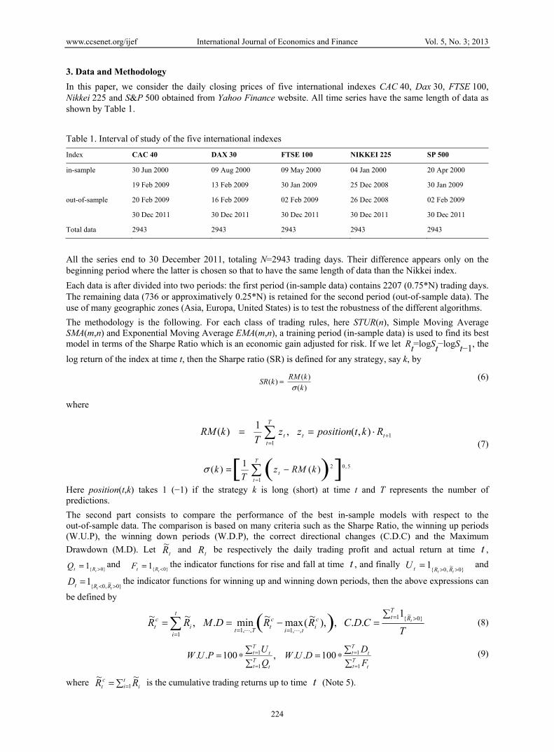
3. Data and Methodology

In this paper, we consider the daily closing prices of five international indexes CAC 40, Dax 30, FTSE 100, Nikkei 225 and S&P 500 obtained from Yahoo Finance website. All time series have the same length of data as shown by Table 1.

Table 1. Interval of study of the five international indexes

Index CAC 40 DAX 30 FTSE 100 NIKKEI 225 SP 500

in-sample 30 Jun 2000 09 Aug 2000 09 May 2000 04 Jan 2000 20 Apr 2000

19 Feb 2009 13 Feb 2009 30 Jan 2009 25 Dec 2008 30 Jan 2009

out-of-sample 20 Feb 2009 16 Feb 2009 02 Feb 2009 26 Dec 2008 02 Feb 2009

30 Dec 2011 30 Dec 2011 30 Dec 2011 30 Dec 2011 30 Dec 2011

Total data 2943 2943 2943 2943 2943

All the series end to 30 December 2011, totaling N=2943 trading days. Their difference appears only on the beginning period where the latter is chosen so that to have the same length of data than the Nikkei index.

Each data is after divided into two periods: the first period (in-sample data) contains 2207 (0.75*N) trading days. The remaining data (736 or approximatively 0.25*N) is retained for the second period (out-of-sample data). The use of many geographic zones (Asia, Europa, United States) is to test the robustness of the different algorithms.

The methodology is the following. For each class of trading rules, here STUR(n), Simple Moving Average SMA(m,n) and Exponential Moving Average EMA(m,n), a training period (in-sample data) is used to find its best model in terms of the Sharpe Ratio which is an economic gain adjusted for risk. If we let Rt=logSt−logSt−1, the

log return of the index at time t, then the Sharpe ratio (SR) is defined for any strategy, say k, by

)(

)()(

k

kRMkSR

(6)

where

1

1

),(,1

)(

ttt

T

t

RktpositionzzT

kRM (7)

5,02

1])([ )(

1)( kRMz

Tk t

T

t

Here position(t,k) takes 1 (−1) if the strategy k is long (short) at time t and T represents the number of predictions.

The second part consists to compare the performance of the best in-sample models with respect to the out-of-sample data. The comparison is based on many criteria such as the Sharpe Ratio, the winning up periods (W.U.P), the winning down periods (W.D.P), the correct directional changes (C.D.C) and the Maximum

Drawdown (M.D). Let tR~

and tR be respectively the daily trading profit and actual return at time t ,

}0{1 tRtQ and

}0{1 tRtF the indicator functions for rise and fall at time t , and finally

}0~

,0{1

tt RRtU and

}0~

,0{1

tt RRtD the indicator functions for winning up and winning down periods, then the above expressions can

be defined by

TCDCRRDMRR tR

Ttc

iti

ct

Tti

t

i

ct

}0~

{1

,,1,,11

1..,),

~(max

~min.,

~~ )(

(8)

tTt

tTt

tTt

tTt

F

DDUW

Q

UPUW

1

1

1

1 100..,100.. (9)

where iti

ct RR

~~1 is the cumulative trading returns up to time t (Note 5).


225

Finally, we integrate the transaction costs in the analysis. Namely, it is supposed that any transaction implies a constant cost of 20 basis points.

4. Results

We recall that the in-sample data contains approximatively 9 years of data for each index. The STUR(n) class, with the constraint 8≤n≤50 and n, n/12 or n/20 is a power of 2, contains height (08) admissible strategies characterized by the integer n valued in {8, 12, 16, 20, 24, 32, 40, 48}. The simple and exponential moving average classes are parametrized by two integers m and n, representing respectively the lead and lag parameter. In this study, sixteen (16) strategies are proposed for each Moving Average class with their parameters given by m∈{1, 5, 10, 15,} and n∈{50, 100, 150, 200}. All these algorithms need some initial data to start the forecasting procedure. For example, the STUR(n) strategy needs n+1 data to make the first forecast. For these initial data, the agent decision is supposed to be always 1. The cost of one transaction is taken to be 20 basis point i.e 0.2%.

Table 2 shows the performance of the best strategies in each class through the different indexes and through their respective in-sample data given in Table 1.

For the STUR class, the best strategy is given by the parameter n=16 for the CAC, NIKKEI and S&P indexes and by n=20 and 24 for the DAX and FTSE indexes, respectively. Overall, it is seen for the STUR class, the approximation needs to be local or to have less data (n≤24) to generate good results.

For the Exponential Moving Average class, the lag parameter of the best strategy is always equal to n=150 for the different indexes and the lead parameter lies to the set {10, 15}. For the Simple Moving Average class, the lag parameter varies through indexes where the parameter n=150 is more frequent. The same remark applies also for the lead parameter m where the mode is given by m=15. We also remark that for both moving average classes, a small lead (m=1 or 5) does not give satisfactory in-sample results. All best competing models (STUR, EMA, SMA), in the in-sample evaluation, generate economic gains or a positive Sharpe Ratio. Furthermore, except in the FTSE index, the optimal strategy of the EMA class outperforms the other best models.

Table 2. Sharpe ratio of the best trading rules in each class (In-sample)

Class STUR(n ) EMA (m,n) SMA(m,n) Buy and Hold

CAC n=16 m=10, n=150 m=15, n=150

Sharpe Ratio 0.45 0.741 0.730 -0,37

Dax n=20 m=15, n=150 m=15, n=150

Sharpe Ratio 0.627 0.7825 0.5974 -0.218

FTSE n=24 m=15, n=150 m=15, n=150

Sharpe Ratio 0.4938 0.451 0.492 -0.210

Nikkei n=16 m=10, n=150 m=10, n=50

Ratio 0.222 0.611 0.528 -0.355

S&P n=16 m=15, n=150 m=15, n=200

Sharpe Ratio 0.274 0.4728 0.4436 -0.2916

On the other hand, the Buy and Hold Strategy has a negative mean in the in-sample data of all geographical zones showing consequently a negative Sharpe ratio. This may be explained by the fact that all five indexes are highly correlated and therefore the probability to have the same sign performance in the five indexes is very high.

After getting the best strategy in each class, we make a comparison between them. Namely, three trading rules are investigated for each index in their out-of-sample data given in Table 1. The aim is to see if it is possible to do better than the benchmark strategy after taking into account transaction costs. To reduce the chance feature, a long time series of out-of-sample is considered as containing around three years of data. The results are shown in the Table 3 and Table 4 .


226

Table 3. Out-of-sample performance of the best trading rules in each class (Part I)

CAC STUR(16) EMA (10,150) SMA(15,150) Buy and Hold

Sharpe Ratio 0.135 -0.72 -0.16 0.125

Transactions 4 20 6 0

M.D -0.35 -0.83 -0.52 -0.40

DAX 30 STUR(20) EMA (15,150) SMA(15,150) Buy and Hold

Sharpe Ratio 0.53 0.13 0.32 0.40


M.D -0.33 -0.42 -0.30 -0.39

FTSE 100 STUR(24) EMA (15,150) SMA(15,150) Buy and Hold

Sharpe Ratio -0.11 -0.29 0.30 0.49


M.D -0.37 -0.34 -0.29 -0.20

Nikkei 225 STUR(16) EMA (10,150) SMA(10,150) Buy and Hold

Sharpe Ratio 0.03 -0.46 -0.77 -0.01


M.D -0.32 -0.59 -0.61 -0.33

S&P 500 STUR(16) EMA (15,150) SMA(15,200) Buy and Hold

Sharpe Ratio 0.09 -0.73 -0.20 0.63


M.D -0.41 -0.66 -0.40 -0.21

Description: This table presents the out-of-sample values of the Sharpe ratio, the number of transactions and the Maximum Drawdown (M.D)

for each best strategy.

Table 4. Out-of-sample performance of the best trading rules in each class (Part II)

CAC 40 STUR(16) EMA (10,150) SMA(15,150)

C.D.C 50.41% 47.83% 50.82%

W.U.P 34.32% 52.82% 57.91%

W.D.P 66.94% 42.70% 43.53%

DAX 30 STUR(20) EMA (15,150) SMA(15,150)

C.D.C 52.58% 51.90% 51.77%

W.U.P 73.26% 77.12% 76.61%

W.D.P 29.39% 23.63 % 23.92%

FTSE 100 STUR(24) EMA (15,150) SMA(15,150)

C.D.C 51.90% 50.27% 50.82%

W.U.P 38.60% 63.73% 60.10 %

W.D.P 66.57% 35.43% 40.57%

Nikkei 225 STUR(16) EMA (10,150) SMA(10,150)

C.D.C 51.90% 52.58% 51.36 %

W.U.P 43.16% 48.16 % 51.32%

W.D.P 61.24% 57.30% 51.40%

S&P 500 STUR(16) EMA (15,150) SMA(15,200)

C.D.C 50.82% 51.63% 53.53%

W.U.P 46.96 % 66.67% 65.21%

W.D.P 55.69% 32.62% 38.77%

Description: This table presents the out-of-sample values of correct directional change (C.D.C), the winning up periods (W.U.P) and the

Winning down periods (W.D.P) for each best strategy.

Table 3 shows that for the Sharpe Ratio criterion, the STUR strategy gives overall the best results, namely three over the five indexes. Then it is followed by the B&H strategy which performs two times over the five cases. The results of SMA and EMA trading rules are not satisfactory in the out-of-sample data.

For the Maximum Drawdown (M.D) measure, it is found over all that the two best strategies are also given by the STUR class and the Buy and Hold Strategy ( 2 over 5 indexes for each). Precisely, the STUR trading rule obtains the good results from the CAC and Nikkei indexes while B&H does better in the FTSE and S&P indexes.

www.ccsen

The more Maximum

It is notedindexes. Fof the otheindex whe

Now, we adirectional

For the Ctrading rulFTSE. Thethe W.U.PHowever, measure wresults and

We can resince it beCorrect dirWinning U

5. Conclus

In this pacontributiomodels. FsimplificatThe first idata used is to solveof the prinof Rn andthe averagpositive (n

net.org/ijef

M.D, the littlem downside and

d that the riskieFor the profitaber strategies fo

ere SMA gives

are interested l changes in th

.D.C criterionle gives bettere EMA, with a

P criterion, it isin financial m

will play a majd sometimes th

Figure 1

sume the analyelongs to the brectional chan

Up period crite

sion

aper, the stochon consists inor this purpostions are also s to constraintin the regressi

e the dimensionncipal componed then associatge forecast of tnegative). To

Inte

e is the downsd profitability (

est strategies (bility measure,or the CAC, Dsome interesti

in the percenthe rise and fall

n, the two besr results for thea C.D.C of 52.s EMA the besmarkets, investjor role for thehe difference is

1. The cumulat

ysis, by sayingbest strategies nge and the Wierion.

hastic unit roon approximatse, two simplirelevant to re

t the stochasticion, the nonlinnality problement analysis (Pte to each vectthese n modelsdiminish the

ernational Journa

ide risk. The c(Sharpe Ratio)

(downside risk, it is also seen

DAX, Nikkei ang results.

tage of correctperiods (W.U.

st strategies are CAC and S&58% only outp

st trading rulestors are more em. It is noteds very significa

tive return path

g overall, the Sfor many criteinning down p

ot model is uting locally thifications are duce the execc parameter to

nearities are apm by extractingPCA) by takingtor, a simple lis and the decistransaction co

al of Economics

227

cumulative retu) over the out-o

k) are usually n that the STUand S&P index

t directional ch.P and W.D.P)

re given by S&P indexes whperforms the o in three over concern to de

d that, for all fant as in the ca

h of the differe

STUR strategyeria such as thperiods. Its poo

used to forecahe nonlinearitimade to facilution time and

o take, at any tpproximated byg only the mosg n orthogonalinear model. Tsion making isosts for profita

s and Finance

turns of Figureof-sample data

reached by SMUR and B&H cxes. The excep

hanges (C.D.C), see the eqs. (

SMA and STUhile the STURther trading ruthe five indice

etect falling pefive indexes, tase of CAC an

ent trading rule

y outperforms he Sharpe ratioor results in th

ast the directiies of financilitate the estimd the memorytime, two possy 2n linear mst significant lil binary vector

Then, the strates simply to buyability reasons

e 1 illustrates ba for the differ

MA and EMA cumulative retption appears

C), and the pe(8) and (9) and

UR. The simplR strategy perfoules for the Nikes and then it ieriods. Conseqthe STUR strand S&P indexe

es for each ind

the moving avo, the Maximuhe out-of-samp

ion change ofial time seriesmation of the y cost involvedsible values. C

models. The secinear models. Wrs (columns ofegy STUR(n) isy (sell) if this s, but also to

Vol. 5, No. 3;

both the concerent indexes.

in four amongturns end at thonly for the F

rcentage of cod Table 4.

le moving aveforms for DAXkkei index. Bus followed by quently, the Wategy gives thes.

dex

verage trading um Drawdownple only come

f asset prices.s by simple lparameters. T

d by the algorConsequently, cond simplificWe follow the

f Hadamard mas defined by taaverage foreccapture signif

2013

ept of

g five e top

FTSE

orrect

erage X and ut, for

SMA. W.D.P e best

rules n, the from

The inear

These ithm. for n ation

e idea atrix) aking ast is ficant


228

informations, an endogenous threshold c is used to activate a decision. Namely, the trader will transact if the average forecast return is superior in absolute value to the threshold, elsewhere the previous position is conserved. It is found that the strategies from STUR class dominate overall the moving average trading rules (simple and exponential) and also the Buy and Hold strategy for the Sharpe criterion.

These interesting results may be explained by two facts. First, it is known that random coefficient autoregressive models are able to fit well financial asset prices. So it is expected to have satisfactory results when this econometric model is used for forecasting. The second reason is due to our estimation procedure which is local and allows to capture feedback or interaction of traders rather using methods based on stationarity assumptions in variance or higher moments that are violated in our case of stochastic unit root model.

References

Dunis, C. L., Williams, M. (2003). Applications of Advanced Regression Analysis for Trading and Investment. C. In L. Dunis, J. Laws & P. Naïm (Eds.), Applied Quantitative Methods for Trading and Investment. John Wiley & Sons.

Granger, C. W. J., & Ramanathan, R. (1984). Improved Methods of Combining Forecasts. Journal of Forecasting, 3, 197-204. http://dx.doi.org/10.1002/for.3980030207

Granger, C. W., & Swanson, N. R. (1997). An introduction to stochastic unit-root processes. Journal of Econometrics, 80, 35-62. http://dx.doi.org/10.1016/S0304-4076(96)00016-4

Konté, M. A. (2011). A link between Random Coefficient AutoRegressive Models and some kind of Agent Based Models. Journal of Economic Interaction and Coordination, 6(1), 83-92. http://dx.doi.org/10.1007/s11403-010-0077-3

Konté, M. A. (2010). Behavioural Finance and Efficent Markets: Is the joint hypothesis really the problem? IUP Journal of Behavioral Finance, 7, 9-19.

Lo, A. (2005). Reconciling Efficient Markets with Behavioral Finance: The Adaptive Markets Hypothesis. Journal of Investment Consulting, 7(2), 21-44.

Nicholls, D. F., & Quinn, B. G. (1982). Random Coefficient Autoregressive Models: An Introduction. Lecture Notes in Statistics, 11. New York: Springer-Verlag. http://dx.doi.org/10.1007/978-1-4684-6273-9

Nicholls, D., & Quinn, B. (1981). The Estimation of Random Coefficient Autoregressive Models. II. Journal of Time Series Analysis, 2, 185-203. http://dx.doi.org/10.1111/j.1467-9892.1981.tb00321.x

Ou, J., & Penman, S. (1989). Accounting measurement, Price-Earnings Ratio, and the information content of security prices. Journal of Accounting Research, 27, 111-152. http://dx.doi.org/10.2307/2491068

Sollis, R., Leybourne, S., & Newbold, P. (2000). Stochastic unit roots modelling of stock price indices. Applied financial economics, 10, 311-315. http://dx.doi.org/10.1080/096031000331716

Sullivan, R., Timmermann, A., & White, H. (1999). Data-snopping, technical trading rule performance, and the boostrap. The journal of finance, 54, 1647-1691. http://dx.doi.org/10.1111/0022-1082.00163

Wang, D., & Ghosh, S. K. (2002). Bayesian Analysis of Random Coefficient Autoregressive Models. Model Assisted Statistics and Applications, 3(2), 281-295.

Yoon, G. (2003). A simple model that generates stylized facts of returns. Department of Economics, UCSD. Paper 2003-04.

Yoon, G. (2006). A note on some properties of STUR processes. Oxford Bulletin of Economics and Statistics, 68, 253-261. http://dx.doi.org/10.1111/j.1468-0084.2006.00161.x

an investment strategy based on stochastic unit root models - copy

Documents