an observational and numerical study of a regional-scale

An observational and numerical study of a regional-scale downslope

flow in northern Arizona

L. Crosby Savage III,1 Shiyuan Zhong,1 Wenqing Yao,1 William J. O. Brown,2

Thomas W. Horst,2 and C. David Whiteman3

Received 19 November 2007; revised 5 February 2008; accepted 20 March 2008; published 22 July 2008.

[1] Boundary layer observations taken during the METCRAX field study in October of2006 near Winslow in Northern Arizona revealed the frequent presence of a near-surfacewind maximum on nights with relatively quiescent synoptic conditions. Data from asodar, a radar wind profiler, several surface stations, and frequent high-resolutionrawinsonde soundings were used to characterize this boundary layer wind phenomenonand its relation to synoptic conditions and the ambient environment. The data analysesare augmented by high-resolution mesoscale numerical modeling. It is found thatthe observed nocturnal low-level wind maximum is part of a regional-scale downslopeflow converging from high terrain of the Colorado Plateau toward the Little ColoradoRiver Valley. The depth of this downslope flow is between 100 and 250 m with apeak speed of 4–6 m s�1occurring usually within the lowest 50 m above ground.Opposing ambient winds lead to a longer evening transition period, shallower slope flows,and a smaller horizontal extent as compared to supporting synoptic winds. A simpleanalytical solution based on local equilibrium appears to agree fairly well with the observedlayer mean downslope wind speed, but the classic Prandtl solution for maximumdownslope wind speed fails to match the observations. The properties of the flow appear tobe insensitive to changes in soil moisture, land cover, and surface roughness length.The contribution to the low-level wind maximum by inertial oscillation at night isfound to be insignificant.

Citation: Savage, L. C., III, S. Zhong, W. Yao, W. J. O. Brown, T. W. Horst, and C. D. Whiteman (2008), An observational and

numerical study of a regional-scale downslope flow in northern Arizona, J. Geophys. Res., 113, D14114,

doi:10.1029/2007JD009623.

1. Introduction

[2] Terrain-induced local or regional circulations are quitecommon within the western United States due to the complextopography and the climatologically dry stable conditions ofthe region. These terrain-induced flows have previously beenobserved along valley sidewalls [Whiteman, 1982], withinbasins [Clements et al., 2003], and down mountain slopes[Horst and Doran, 1986]. Such observations lead to impor-tant discoveries of the characteristics and consequences ofdownslope flows within all types of topographic environ-ments. Alexandrova et al. [2003] found a striking correlationbetween the thermally driven slope flow around Salt LakeCity, UT and the fluctuation of aerosol particles of diameterless than 10micronswithin the city. A similar study inMexicoCity found that a nocturnal downslope flow was the maincause of an increase in ozone concentrations within theheavily populated urban area [Raga et al., 1999]. Smith et

al. [1997] has pointed to the consequences of slope flows asan obstacle in transportation management, land use planning,and air pollution management for determining the environ-mental and economical impacts upon a region.[3] Observational studies have shown the characteristics of

nocturnal downslope flows vary with slope angle, slopelength, surface type, ambient winds, and stability. Manyinvestigators have used analytical and numerical models tocharacterize the structure and evolution of downslope flowsand to relate them to the ambient or large scale atmosphericconditions. Prandtl [1942] was one of the first to develop atheoretical model for describing the vertical structure ofdownslope flow. Prandtl’s model gives the height and speedof the downslope jet as a function of the stability, slope angle,and eddy diffusivity. Mahrt [1982] examined the forcingmechanisms behind downslope flows by carefully evaluatingthe relative roles of terms in the momentum and thermody-namic equations in a slope following coordinate. Theseanalytical studies have provided a basis for understandingthe different observed characteristics of downslope flows indifferent environments.[4] Recent studies have focused more on the interaction

of downslope flow with dynamical forces at different scales.Idealized numerical simulations have examined the impactof slope shape. Smith and Skyllingstad [2005] found that

JOURNAL OF GEOPHYSICAL RESEARCH, VOL. 113, D14114, doi:10.1029/2007JD009623, 2008ClickHere

for

FullArticle

1Department of Geography, Michigan State University, East Lansing,Michigan, USA.

2Earth Observing Laboratory, National Center for AtmosphericResearch, Boulder, Colorado, USA.

3Department of Meteorology, University of Utah, Utah, USA.

Copyright 2008 by the American Geophysical Union.0148-0227/08/2007JD009623$09.00

D14114 1 of 17

http://dx.doi.org/10.1029/2007JD009623

slopes with a concave shape have a stronger accelerationnear the top of the slope which then transitions toward aslower more elevated jet near the base. Uniform slopes, onthe other hand, were found to maintain a constant profile ofdownslope flow along the slope, with stronger accelerationsnear the base. Other idealized studies have demonstrated theimportance of inhomogeneous surface parameters along theslope [Shapiro and Fedorovich, 2007], and the impact ofopposing synoptic scale flow, which affects the depth andstrength of the downslope flow [Arritt and Pielke, 1986].Along with these idealized studies, observational and lab-oratory studies have examined downslope flows over smallslopes [Soler et al., 2002], slope discontinuities [Fernandoet al., 2006], the impact of downslope flow upon turbulence[Van Der Avoird and Duynkerke, 1999; Monti et al., 2002],and the interaction of downslope flows with larger scalephenomena, such as mountain waves [Poulos et al., 2000].While analytical, numerical, and laboratory studies haveaided the understanding of downslope flow, field observa-tions have provided a vital validation to theoretical findings.Previous observational studies have been carried out overisolated small-scale slopes only a few kilometers in length[Doran et al., 2002; Horst and Doran, 1986; Haiden andWhiteman, 2005], or at larger scales in the pole regions ofAntarctica [Renfrew and Anderson, 2006; Heinemann andKlein, 2002]. This has lead to a limited understanding ofdownslope flows along larger scale slopes and their inter-actions with synoptic forcing in midlatitude regions.[5] In October 2006, the Meteor Crater Experiment, or

METCRAX, was launched to investigate the evolution ofthe stable boundary layer and the formation of atmosphericseiches in Arizona’s Meteor Crater approximately 60 kmeast southeast of Flagstaff, AZ. Observations were madeboth inside and outside Meteor Crater to document the

interaction of the temperature structure and wind inside thecrater with the ambient flows and stability conditions.Observations outside the Meteor Crater found frequentnear-surface nocturnal wind maxima (4–6 m s�1). Thesenocturnal near-surface wind maxima were associated withsouthwesterly winds which, based on the topography at thesite, were likely to be downslope flows. Little is known,however, about the horizontal extent or scale of this down-slope flow, its evolution with time, its depth, and how itscharacteristics, such as onset time, peak speed, depth etc.,change with synoptic conditions. The METCRAX observa-tions afforded a unique opportunity to answer these ques-tions. This paper combines METCRAX observations witha mesoscale numerical model to characterize this windphenomenon and its interaction with larger-scale forcing.Section 2 describes in more detail the site and measure-ments while section 3 describes the relevant observations.Section 4 introduces numerical model simulations and theirresults. Finally, conclusions are drawn in section 5.

2. Sites, Instrumentation, and Measurements

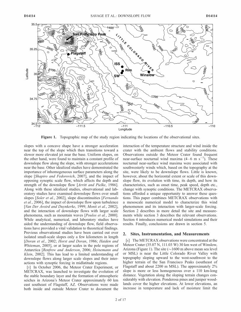
[6] TheMETCRAX observations were concentrated at theMeteor Crater (35.07 N, 111.03 W) 30 km west of Winslow,Arizona (Figure 1). The site (�1600 m above mean sea levelor MSL) is near the Little Colorado River Valley withtopography sloping upward to the west-southwest to thehigher terrain of the San Francisco Peaks (southeast ofFlagstaff and about 2200 m MSL). The approximately 2%slope is more or less homogeneous over a 110 km-longdistance. Vegetation along the sloping terrain changes con-siderably with elevation. Ponderosa pines and juniper wood-lands cover the higher elevations. At lower elevations, anincrease in temperature and lack of moisture limit the

Figure 1. Topographic map of the study region indicating the locations of the observational sites.

D14114 SAVAGE ET AL.: DOWNSLOPE FLOW

2 of 17

D14114

vegetation to prairie grassland and small desert shrubs.Climate within the region is typical of much of the south-western United States, which is dominated by subsidencefrom high pressure ridging more than 70% of days in bothsummer and early fall seasons [Wang and Angell, 1999]. Thisclimatic pattern of clear, stable conditions makes the regionespecially susceptible to terrain-induced circulations.[7] To accurately observe the circulation along the slope,

three observational sites were installed at various locations.The first was 5 km north-northwest of Meteor Crater. Thissite was equipped with the National Center for AtmosphericResearch (NCAR)’s Integrated Sounding System (ISS),which consisted of an enhanced surface weather station, a915-MHz radar wind profiler with Radio Acoustic Sound-ing System (RASS), and a rawinsonde sounding system.Vaisala RS-92 GPS sondes were launched on seven Inten-sive Observational Periods (IOPs) during the month-longexperiment and the launches would start at 1500 LST and

continue until 0900 LST the next morning at 3 hourlyintervals. This site will hereafter be referred to as the ISS site.A second measurement site (henceforth designated the SWsite) was located 2.5 km southwest of Meteor Crater. The sitehad a 10-m weather tower and a mini Sodar (MetekDSDPA.90-24) with RASS that measured wind speed anddirection and temperature continuously from 40 m aboveground to about 200 m aloft at 20 m vertical resolution. Thethird site was on the northwest rim of Meteor Crater (hence-forth Rim site) where a 10-m tripod was installed withtemperature and humidity sensors (Vaisala 50Y) mounted attwo levels (2 m and 10 m) and a R. M. Young propeller vanewind monitor at the 10 m level.[8] The general behavior of near-surface winds during the

month-long experiment can be seen by the wind roses andfrequency distribution at the ISS site for the entire month ofthe experiment in Figure 2 for both nighttime and daytime.Dominating the nighttime period over fifty percent of the

Figure 2. Wind roses and frequency distributions for the 10-m wind at the ISS site for October 2006.


3 of 17

D14114

time is a terrain-following southwesterly flow with a fre-quent speed of 4 to 5 m s�1. The daytime period also showsa high frequency from the southwest, though a small peakfrom the north-northeast possibly exemplifies the effects ofa weak upslope component. Strong surface winds exceeding8 m s�1 were caused by downward mixing of strongsynoptic winds during daytime.[9] In this study, surface and upper air observations from

three of the seven METCRAX IOPs (IOP 4, 5, 6) are used

to investigate the detailed characteristics of the nocturnaldownslope flow and its interactions with synoptic condi-tions. The three IOPs were selected to provide a range ofdifferent synoptic wind directions and speeds.

3. Observed Downslope Flow Characteristics

3.1. Synoptic Conditions

[10] The synoptic conditions for the three IOPs aredescribed in this section. IOP 6 (28–29 October) was

Figure 3. 0500LST500-mbgeopotential height fields andwindvectors for (a) IOP 6, 29October, (b) IOP5,23 October, and (c) IOP 4, 21 October, based on North American Regional Reanalysis (NARR) data.


4 of 17

D14114

characterized by weak ambient winds from the southwest,allowing downslope flow to develop over the region.Synoptic conditions were dominated by a ridge of highpressure between a digging trough in the Great Plains and aweak cutoff low-pressure system off the coast of California(Figure 3a). This allowed weak winds aloft to develop overnorthern Arizona through most of the night before givingway the next morning to a southerly jet. The weak ambientwinds were typical of downslope development throughoutthe month, though the ambient wind direction was notalways from the southwest.[11] IOP 5 (22–23 October) was characterized by a low-

level easterly jet, or opposing ambient wind to the south-westerly downslope flow. The easterly flow occurred as alow level jet between 700 and 900 m above ground level asthe cutoff low aloft pushed a surface trough into NorthernArizona (Figure 3b). Above the easterly wind layer andsimilar to IOP 6, the synoptic winds aloft at 500 hPa wererelatively weak at 5 to 10 m s�1 from the south or southwest(Figure 3b). This easterly low-level jet opposes the south-westerly downslope flow, contributing to the differences inthe observed downslope flows between this night and thenight of IOP6 when the midlevel large-scale winds were inthe same direction as the downslope flow.

[12] As synoptic conditions aloft strengthened and strongwinds began to mix down to the surface, the signaturesof terrain-induced circulations became weaker and some-times disappeared all together. An example of synopticforcing overpowering local forcing is given in IOP 4(20–21 October) in Figure 3c. On this night, a diggingtrough developing just to the north of the region broughtstrong northwesterly winds to the study area. The strongwinds began to mix to the surface, which limited theimpact of the terrain-induced circulation.

3.2. Time Variations of the Downslope Flow

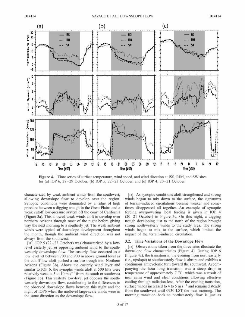
[13] Observations taken from the three sites illustrate thedownslope flow characteristics (Figure 4). During IOP 6(Figure 4a), the transition in the evening from northeasterly(i.e., upslope) to southwesterly flow is abrupt and exhibits acontinuous anticyclonic turn toward the southwest. Accom-panying the hour long transition was a steep drop intemperature of approximately 7 �C, which was a result ofnear calm wind and clear conditions allowing effectivecooling through radiation loss. After the evening transition,surface winds increased to 4 to 5 m s�1 and remained steadyfrom the southwest until 0930 LST the next morning. Themorning transition back to northeasterly flow is just as

Figure 4. Time series of surface temperature, wind speed, and wind direction at ISS, RIM, and SW sitesfor (a) IOP 6, 28–29 October, (b) IOP 5, 22–23 October, and (c) IOP 4, 20–21 October.


5 of 17

D14114

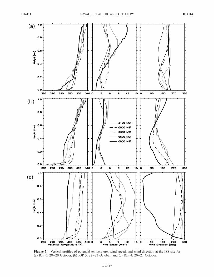
Figure 5. Vertical profiles of potential temperature, wind speed, and wind direction at the ISS site for(a) IOP 6, 28–29 October, (b) IOP 5, 22–23 October, and (c) IOP 4, 20–21 October.


6 of 17

D14114

abrupt as the onset of the downslope flow; occurring withinan hour and accompanied with weak surface winds.[14] Surface observations taken from IOP 5 show similar

patterns to those observed during IOP 6 with a change inwind direction after sunset to the southwest (Figure 4b). Themain difference between the supporting ambient flow ofIOP 6 and the opposing ambient flow of IOP 5 was theevening transition period. The evening transition of IOP 5took two hours longer than IOP 6 and exhibited a cyclonicshift, turning continuously from easterly flow during theday to northerly, and finally stopping with a southwesterlydownslope flow. This agrees with the theoretical modelfindings of Fitzjarrald’s [1984] of delayed onset time withopposing ambient flow. The longer transition was alsoaccompanied by weak winds near the surface and a tem-perature decrease of near 7 �C. Overnight, the surface windswere again characterized by a steady flow from the south-west averaging 4 m s�1. The morning transition back tosynoptically driven or possibly upslope flow, exhibited the

same characteristics as in IOP 6, though the transitionoccurred slightly earlier at 0810 LST.[15] IOP 4 exhibited a shift in wind direction at the

surface from easterly during the day to westerly at night,but the characteristics of the transition and flow are notcomparable to the previous downslope flow examples(Figure 4c). Instead, the easterly winds during the daybegan to transition to a southwest direction before sunset.During previous IOPs, the downslope transition wasaccompanied by a decrease in near-surface wind speedand a rapid drop in temperature, but for IOP 4 the eveningtransition was characterized by increasing wind speeds andlittle temperature change near the surface. As the nightprogressed, the winds continued to slowly shift morewesterly and eventually, after 0300 LST, became northwest-erly, which was the same as the ambient flow direction aloft.Surface wind speeds during the period were also strongerand more variable in magnitude ranging from near 4 m s�1

to almost 10 m s�1. The strong synoptic forcing is thusdriving the surface winds, limiting the impacts of theterrain-induced circulation.

3.3. Vertical Structure of the Downslope Flow

[16] The vertical structure of the downslope flow wasdetermined from 3-hourly rawinsonde soundings from theISS site and from 1-h mean sodar observations at the SWsite. Figure 5a illustrates the time sequence of the IOP 6soundings, which were characterized by stable conditionsaloft and a strong surface temperature inversion in thelowest 20 to 30 m above ground level (AGL) from2100 LST on 28 October till 0600 LST the next morning.Accompanying the inversion was a near-surface windmaximum of 4 to 5 m s�1, with wind speed weakeningwith height up to 200 m AGL. During the morningtransition (around 0900 LST) the near-surface wind maxi-mum disappeared as a growing convective boundary layereroded the overlying temperature inversion and began toexhibit greater influence from larger scale forcing. From the

Figure 6. Hourly wind vectors from the Sodar and surfaceobservations at the SW site for (a) IOP 6, 1800 LST 28October – 0700 LST 29 October (b) IOP 5, 1800 LST 22October – 0700 LST 23 October, and (c) IOP 4, 1800 LST20 October – 0700 LST 21 October.

Figure 7. Comparison of observed layer-averaged down-slope wind speed by the rawinsonde soundings at the ISSsite with those predicted by the analytical equilibriumsolution.


7 of 17

D14114

rawinsonde profile, it is difficult to determine the down-slope flow layer depth, but the combined hourly sodar and10-m surface observations taken at the SW site provide adetailed picture of the change in downslope flow depthduring the night (Figure 6a). At first, the downslope flowwas shallow and weak, but by midnight the depth andstrength of the flow was at its peak. Consistent with the0000 LST sounding, the southwesterly downslope flowextended up to 120 m AGL. Later in the night, the depthof the downslope flow began to decrease to below 100 mAGL, and after sunrise was limited to the first 10s of metersAGL. The fluctuation of the depth of the downslope flowthroughout the night makes definitive determination of theheight of the flow difficult, though a range of 50 to 150 mabove AGL would best describe the downslope flow forIOP 6.[17] The effect of easterly ambient winds on the down-

slope flow is illustrated through the series of three-hourlyvertical sounding profiles taken during IOP 5 (Figure 5b).The soundings again showed a typical terrain-driven south-westerly flow with maximum speed close to the surface, anda strong inversion of almost 10 K just above the surface.The morning transition around 0900 LST was similar toIOP 6, as the winds near the surface were significantlyweaker and increased with height. A closer examination ofthe sounding and sodar observations for IOP 5 shows afluctuating depth between 50 and 100 m, with the maxi-mum depth noticeably lower than that in IOP 6 (Figure 6b).Similar to IOP 6, though, is an increase in depth overnightfrom about 10 m at the beginning of the night, to about 70 mby 0200 LST.[18] The effects of the strong synoptic northwesterly flow

from IOP 4 are seen in the vertical profiles of the 3-hourlysoundings (Figure 5c). Unlike the previous IOPs, there wasno wind maximum near the surface, but instead the windsincreased with height and were predominantly from thenorthwest. The temperature inversion on this night was alsomuch weaker compared to the other nights. The sodarobservations taken from IOP 4 illustrate the strong influenceof the synoptic northwest flow, as there is little evidence ofterrain-induced drainage flow at any depth throughout thenight (Figure 6c).

3.4. Comparison With Analytical Solutions

[19] A number of analytical solutions have been proposedto describe the characteristics of downslope flows [Maninsand Sawford, 1979; Kondo and Santo, 1988; Nappo andRao, 1987; Mahrt, 1982]. Most of these are simplifiedsolutions of the bulk momentum equation for downslopeflows

@

@th�uþ @

@xhu2 ¼ g

qoh�q sina� g

qocosa

@

@xh2 ��qþto � th ð1Þ

Equation (1) is obtained by integrating the momentumequation in a slope-following coordinate system

@u

@tþ u

@u

@xþ v

@u

@yþ w

@u

@z¼ � 1

ro

@p

@xþ g

qqo

sinaþ fv� @w0u0

@z

ð2Þ

from the ground surface to the top of the slope flowlayer with the assumption that hydrostatic equilibriumg qq0cosa = �1

r@p@z exits in the direction perpendicular to slope

surface.[20] In equation (1) and equation (2), u is the downslope

wind component, a is the slope angle, h is the downslopeflow depth, g is the gravity, q0 is the horizontally homoge-neous basic state potential temperature, q is the perturbationpotential temperature or the heat deficit, and t0 � th isturbulent stress divergence across the slope flow layer, whichis typically parameterized by t0 � th =�(CD + k)�u2 with CD

being the surface drag coefficient and k the frictional forcedue to momentum exchange at the interface between thedownslope flow layer and the ambient atmosphere. Theoverbar in equation (1) is the layer mean of a variable

defined by �8 ¼ 1h

Rh0

8(z)dz; while the double bar is the layer

mean of an integral from level z in the slope flow layer to the

top of the layer, ��8 ¼ 1h2

Rh0

dzRhz

8ðz0Þdz0.

[21] A simple analytical solution for downslope windspeed under the condition of local dynamical equilibriumwas proposed by several investigators [Ball, 1956; Kondoand Santo, 1988; Mahrt, 1982]. Under local equilibrium,buoyancy is balanced by turbulent stress divergence andequation (1) is simplified to

g

q0h�q sin a ¼ CD þ kð Þ�u2 ð3Þ

Solving for layer averaged wind speed gives

�u ¼ffiffiffiffiffiffiffiffiffiffiffiffiffiffiffiffiffiffiffiffiffiffiffiffiffiffiffiffiffiffiffiffiffiffiffiffiffiffiffiffiffig

qoh�q sina= CD þ kð Þ

rð4Þ

Figure 8. Comparison of observed maximum downslopewind speed observed by the 3-hourly rawinsonde sound-ings at the ISS site with those predicted by the Prandtlsolution.


8 of 17

D14114

Using nighttime radiosonde profiles launched from the ISSsite during IOPs, the layer-averaged downslope wind speedsare estimated using equation (4) and the results are comparedto those computed directly from the observed downslopewind components (Figure 7). A value of CD + k = 0.008 isused in the computation to satisfy the assumption for localequilibrium that F(CD + k)/sin a = O(1) where F is theFroude number defined as F ¼ �u2

g0h with g0 ¼ g�qq0being the

reduced gravity indicating the relative importance oftransport and Coriolis force terms compared to the buoyancyand thermal wind term. The comparison shows that exceptfor the two disturbed IOPs (IOP 2 and IOP 4) when theambient winds became relatively strong after midnight, theaverage downslope wind speeds predicted by the localdynamical equilibrium theory fairly agrees with the observedvalues. In addition to explaining the differences betweenIOPs, the analytical solution also captures the variationswithin IOP 5 and IOP 6, which were the two best IOPs withquiescent synoptic conditions and well-developed down-slope flows. The results here indicate that under weaksynoptic forcing, the observed downslope flows weregoverned largely by local equilibrium between the buoyancyforce associated with the temperature deficit and turbulentfriction. Nocturnal downslope winds observed over arelatively uniform, low-angle slope (�1.6�) in Salt LakeValley were also found to be in local equilibrium [Whiteman

and Zhong, 2008; Zhong and Whiteman, 2008]. Under suchcircumstance, the simple analytical solution given byequation (4) may be used to predict the mean downslopewind speed.[22] The rawinsonde observations were also used to

evaluate the well-known Prandtl [1942] equilibrium solu-tion for the maximum wind speed in downslope jets.Prandtl’s solution employs eddy diffusivities and a simplethermodynamic equation where diffusion of heat is bal-anced by temperature advection associated with the basicstate stratification. Under such an assumption, the maxi-mum jet speed becomes linearly proportional to the tem-perature deficit at the surface, i.e.,

umax ¼ 0:322Dqsfc

ffiffiffiffiffiffiffiffiffiffiffiffiffiffiffiffiffiffiffiffiffiffiffiffiffiffiffiffiffiffiffig

q0

dq0dz

� ��1Kh

Km

sð5Þ

where Dqsfc is the surface potential temperature deficit, q0represents ambient potential temperature, and Kh, Km areeddy diffusivities for heat and momentum. equation (5)indicates that the speed of the downslope jet increaseslinearly with increasing temperature deficit at the surfaceand increases with weakening ambient stratification.[23] Figure 8 shows a comparison of the observed maxi-

mum downslope wind speed and the estimated maximum

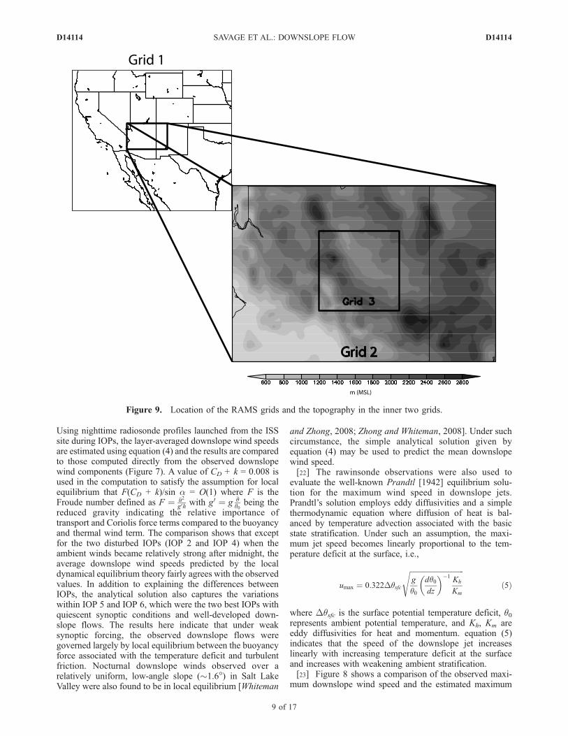
Figure 9. Location of the RAMS grids and the topography in the inner two grids.


9 of 17

D14114

wind speed using the Prandtl solution described by equation(5) based on the nighttime rawinsonde soundings for IOPs 1–6. The calculation assumes that Kh = Km in equation (5). Theplot shows relatively large scatter, suggesting that the Prandtlsolution is not very accurate in predicting the observeddownslope jet. It is interesting to note that the Prandtlsolution appears to be in better agreement with observationsduring the disturbed IOP 2 than with the quiescent IOPs 5and 6. For IOPs 5 and 6, the analytical values are consis-tently higher than the observed values. Detailed analysesindicate that the clear sky and near calm conditions duringthe nights of IOPs 5 and 6 allowed for strong radiationalcooling on the ground and the lack of mixing limited thecooling to a very shallow layer. Consequently, the potentialtemperature deficit at the surface Dqsfc is very large, whichleads to a much larger umax than the actual observed jetmaximum. A better agreement may be achieved by replacingthe surface potential temperature deficit with an averagevalue across a shallow near-surface layer.

4. Numerical Modeling

4.1. Model Setup

[24] The observations captured the temporal variation andthe vertical structure of the downslope flows. Unfortunately,the observations were limited to a few closely located sites

and were unable to document the spatial extent of thisdownslope flow. To better examine the extent of thedownslope flow beyond the limited observational sites,the Regional Atmospheric Modeling System (RAMS[Pielke et al., 1992]), a nonhydrostatic primitive equationmesoscale model in a terrain-following coordinate system,was employed to simulate these IOPs. Subgrid-scale turbu-lent diffusion is parameterized using a level-2.5 scheme[Mellor and Yamada, 1982], which allows a turbulentexchange across the jet maximum and a smooth transitionbetween stable and unstable regimes. Turbulent sensible andlatent heat fluxes and momentum fluxes in the surface layerare evaluated based on the formulation of Louis’s [1979].Radiative heating and cooling were represented by the Chenand Cotton [1983] short- and long-wave radiation schemes,which consider the effect of clouds but do not include theeffects of aerosols on radiation.[25] To accurately represent both the synoptic forcing and

local forcing within the region three two-way interactivenested grids with horizontal grid spacing of 32 km, 8 km,and 2 km were used. The outer grid contained most of thewestern United States and portions of Mexico and thePacific Ocean, the second grid consisted of most of Arizonaand western part of New Mexico, and finally, the innermostgrid covers north-central Arizona including the Little Col-

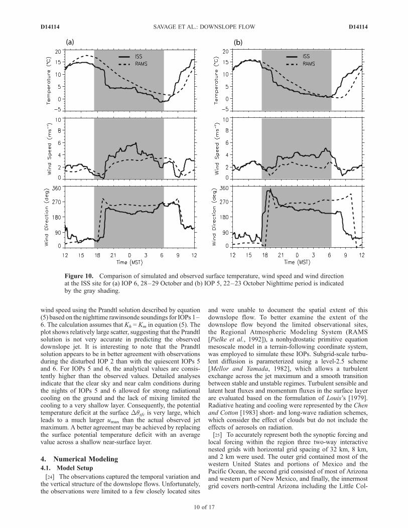
Figure 10. Comparison of simulated and observed surface temperature, wind speed and wind directionat the ISS site for (a) IOP 6, 28–29 October and (b) IOP 5, 22–23 October Nighttime period is indicatedby the gray shading.


10 of 17

D14114

Figure

11.

Sim

ulatedverticalprofiles(left)ofpotential

temperature,windspeed,andwinddirectionat

theISSsite

and

difference

(right)from

observationsofpotential

temperature,uwind,andvwindfor(a)IO

P6,28–29October,(b)IO

P5,

22–23October.


11 of 17

D14114

orado River Valley and the 3800 m San Francisco Peaks(Figure 9). Each grid had 35 vertical levels, stretching from20 m near the surface to 1000 m above 10 km. Thesimulations were initialized at 1200 UTC (0500 LST) usingoutput from the National Center for Environmental Predic-tion (NCEP)’s North American Model (NAM) and eachsimulation ran for 31 h to end at 1900 UTC (1200 LST) thefollowing day.[26] The goal of the model simulations was to provide a

more detailed look at the horizontal and vertical extent of thedownslope flow and how its characteristics change from oneday to the next. For this reason simulations were performedfor the two best IOP nights, IOP 5 (22–23 October) and IOP6 (28–29 October), when synoptic forcing was weak and thedownslope flows were well developed.

4.2. Simulation Results and Discussion

[27] The simulated downslope flow characteristics werefirst compared with the observations for the two IOPs. Asshown in Figure 10, the model was able to capture the majorobserved differences between the two IOPs. For IOP 6, thesimulated evening and morning transitions occurred at thesame time as observed and the simulated anticyclonic shiftalso occurred within an hour, as it did in the observations.

The evening transition of IOP 5 is also well simulated bythe model, as the transitional period to downslope flowtakes longer than IOP 6 and exhibits more of a cyclonicshift. The simulations also adequately captured the drop inwind speed at the surface at the time of transition todownslope for both IOPs, though the simulated near surfacetemperature was warmer than observed. After the transitionthe simulated wind speeds increased overnight, as observed,but were 1 m s�1 less than observations. The discrepancybetween the simulated wind direction that was more west-erly and the observed direction that was southwesterly maybe attributed to the relatively coarse 30’ DEM topographydata set used by the simulations as well as the relativelycoarse model grid resolution.[28] Soundings taken from the two simulations are com-

parable to their observed counterparts at the ISS site(Figure 11). The simulated vertical structure and evolutionof potential temperature are in good agreement with obser-vations, although the simulated surface-based inversion isweaker in the model. Both the simulation and the observa-tions show a low-level wind maximum with wind speeddecreasing with height between 200 and 400 m and in-creasing above, but the observed wind maximum is near theground while the simulated winds peak around 50 m above

Figure 12. Simulated near-surface wind vectors and topography contours in the innermost grid for(a) IOP 6, 28–29 October (b) IOP 5, 22–23 October The triangle indicates the location of the ISS site.


12 of 17

D14114

the ground. The discrepancy between the observed andsimulated height of the wind maximum can be attributedpartially to relatively poor vertical resolution and partially tothe tendency of RAMS to produce stronger mixing near thesurface during nighttime [Zhong and Fast, 2003; Berg andZhong, 2005; Fast and Zhong, 1998]. The vertical winddirection profiles are quite similar to the observations,though slight variations occur near changes of wind direc-tion. IOP 6 is 100 m higher in representing the weaksoutherly wind seen at 200 m in the observations. IOP 5has a better handle on the height of the change in winddirection, but the simulated results show a northern turn inwind direction with height as opposed to the more southerlyturn that was actually observed.[29] Figure 12 shows the simulated near-surface wind

vectors in the innermost model domain at 0000 LST whenthe observations indicated fully developed downslope flowsfor both IOPs. The simulations also exhibit well-developeddownslope flows at the observational sites and it is clear that

this observed downslope flow is part of regional-scale,diurnally varying terrain-induced circulation that convergesfrom high terrains into the Little Colorado River Valleyregion at night and diverges out of the valley toward highterrain during daytime (not shown). The downslope flow inIOP 6 is noticeably stronger and extends further into theLittle Colorado River Valley than IOP 5, which is hamperedby stronger ambient flow and the easterly jet aloft. Alsonoticeable are the increased wind speeds on the other side ofthe valley, which may be enhanced by the easterly jet andmay play a role in producing a smaller horizontal extent ofsouthwesterly downslope flow for IOP 5.[30] The simulated u-components on an east-west ver-

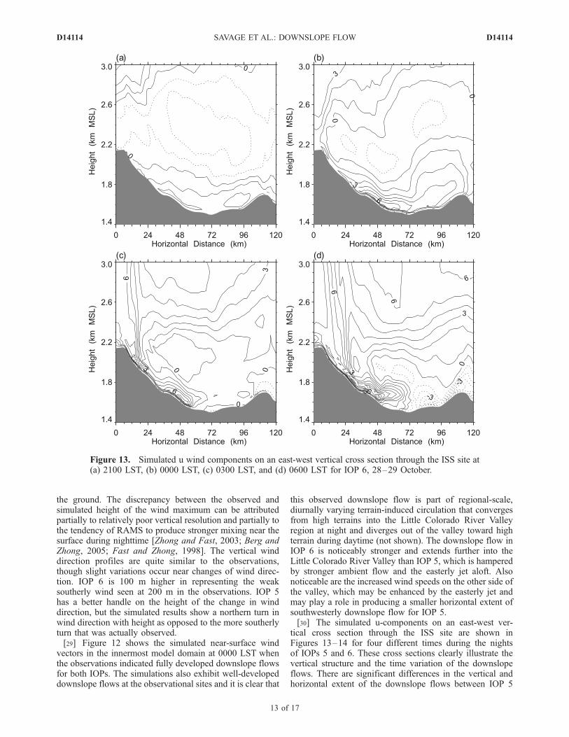
tical cross section through the ISS site are shown inFigures 13–14 for four different times during the nightsof IOPs 5 and 6. These cross sections clearly illustrate thevertical structure and the time variation of the downslopeflows. There are significant differences in the vertical andhorizontal extent of the downslope flows between IOP 5

Figure 13. Simulated u wind components on an east-west vertical cross section through the ISS site at(a) 2100 LST, (b) 0000 LST, (c) 0300 LST, and (d) 0600 LST for IOP 6, 28–29 October.


13 of 17

D14114

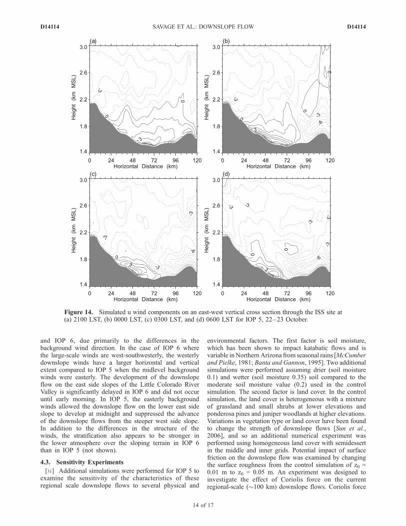
and IOP 6, due primarily to the differences in thebackground wind direction. In the case of IOP 6 wherethe large-scale winds are west-southwesterly, the westerlydownslope winds have a larger horizontal and verticalextent compared to IOP 5 when the midlevel backgroundwinds were easterly. The development of the downslopeflow on the east side slopes of the Little Colorado RiverValley is significantly delayed in IOP 6 and did not occuruntil early morning. In IOP 5, the easterly backgroundwinds allowed the downslope flow on the lower east sideslope to develop at midnight and suppressed the advanceof the downslope flows from the steeper west side slope.In addition to the differences in the structure of thewinds, the stratification also appears to be stronger inthe lower atmosphere over the sloping terrain in IOP 6than in IOP 5 (not shown).

4.3. Sensitivity Experiments

[31] Additional simulations were performed for IOP 5 toexamine the sensitivity of the characteristics of theseregional scale downslope flows to several physical and

environmental factors. The first factor is soil moisture,which has been shown to impact katabatic flows and isvariable in Northern Arizona from seasonal rains [McCumberand Pielke, 1981; Banta and Gannon, 1995]. Two additionalsimulations were performed assuming drier (soil moisture0.1) and wetter (soil moisture 0.35) soil compared to themoderate soil moisture value (0.2) used in the controlsimulation. The second factor is land cover. In the controlsimulation, the land cover is heterogeneous with a mixtureof grassland and small shrubs at lower elevations andponderosa pines and juniper woodlands at higher elevations.Variations in vegetation type or land cover have been foundto change the strength of downslope flows [Sun et al.,2006], and so an additional numerical experiment wasperformed using homogeneous land cover with semidessertin the middle and inner grids. Potential impact of surfacefriction on the downslope flow was examined by changingthe surface roughness from the control simulation of z0 =0.01 m to z0 = 0.05 m. An experiment was designed toinvestigate the effect of Coriolis force on the currentregional-scale (�100 km) downslope flows. Coriolis force

Figure 14. Simulated u wind components on an east-west vertical cross section through the ISS site at(a) 2100 LST, (b) 0000 LST, (c) 0300 LST, and (d) 0600 LST for IOP 5, 22–23 October.


14 of 17

D14114

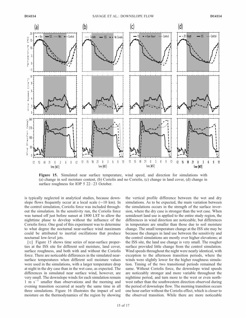
is typically neglected in analytical studies, because down-slope flows frequently occur at a local scale (�10 km). Inthe control simulation, Coriolis force was included through-out the simulation. In the sensitivity run, the Coriolis forcewas turned off just before sunset at 1800 LST to allow thenighttime phase to develop without the influence of theCoriolis force. One goal of this experiment was to determineto what degree the nocturnal near-surface wind maximumcould be attributed to inertial oscillations that producenocturnal low-level jets.[32] Figure 15 shows time series of near-surface proper-

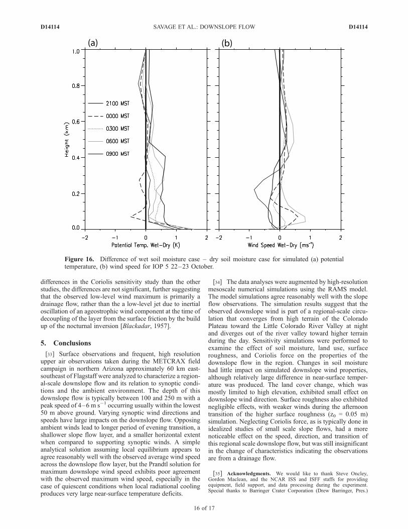
ties at the ISS site for different soil moisture, land cover,surface roughness, and both with and without the Coriolisforce. There are noticeable differences in the simulated near-surface temperatures when different soil moisture valueswere used in the simulations, with a larger temperature dropat night in the dry case than in the wet case, as expected. Thedifferences in simulated near surface wind, however, arevery small. The downslope winds for each simulation remain1 m s�1 smaller than observations and the morning andevening transition occurred at nearly the same time in allthree simulations. Figure 16 illustrates the impact of soilmoisture on the thermodynamics of the region by showing

the vertical profile difference between the wet and drysimulations. As to be expected, the main variation betweenthe simulations occurs in the strength of the surface inver-sion, where the dry case is stronger than the wet case. Whensemidesert land use is applied to the entire study region, thedifferences in wind direction are noticeable, but differencesin temperature are smaller than those due to soil moisturechange. The small temperature change at the ISS site may bebecause the changes in land use between the sensitivity andthe control simulations are mostly over higher elevations; atthe ISS site, the land use change is very small. The roughersurface provided little change from the control simulation.Wind speeds throughout the night were nearly identical, withexception to the afternoon transition periods, where thewinds were slightly lower for the higher roughness simula-tion. Timing of the two transitional periods remained thesame. Without Coriolis force, the downslope wind speedsare noticeably stronger and more variable throughout thenighttime period, and turn more to the west or even north-west rather than the southwestern direction observed duringthe period of downslope flow. The morning transition occursone hour earlier without the Coriolis effect, which is closer tothe observed transition. While there are more noticeable

Figure 15. Simulated near surface temperature, wind speed, and direction for simulations with(a) change in soil moisture content, (b) Coriolis and no Coriolis, (c) change in land cover, (d) change insurface roughness for IOP 5 22–23 October.


15 of 17

D14114

differences in the Coriolis sensitivity study than the otherstudies, the differences are not significant, further suggestingthat the observed low-level wind maximum is primarily adrainage flow, rather than the a low-level jet due to inertialoscillation of an ageostrophic wind component at the time ofdecoupling of the layer from the surface friction by the buildup of the nocturnal inversion [Blackadar, 1957].

5. Conclusions

[33] Surface observations and frequent, high resolutionupper air observations taken during the METCRAX fieldcampaign in northern Arizona approximately 60 km east-southeast of Flagstaff were analyzed to characterize a region-al-scale downslope flow and its relation to synoptic condi-tions and the ambient environment. The depth of thisdownslope flow is typically between 100 and 250 m with apeak speed of 4–6 m s�1 occurring usually within the lowest50 m above ground. Varying synoptic wind directions andspeeds have large impacts on the downslope flow. Opposingambient winds lead to longer period of evening transition, ashallower slope flow layer, and a smaller horizontal extentwhen compared to supporting synoptic winds. A simpleanalytical solution assuming local equilibrium appears toagree reasonably well with the observed average wind speedacross the downslope flow layer, but the Prandtl solution formaximum downslope wind speed exhibits poor agreementwith the observed maximum wind speed, especially in thecase of quiescent conditions when local radiational coolingproduces very large near-surface temperature deficits.

[34] The data analyses were augmented by high-resolutionmesoscale numerical simulations using the RAMS model.The model simulations agree reasonably well with the slopeflow observations. The simulation results suggest that theobserved downslope wind is part of a regional-scale circu-lation that converges from high terrain of the ColoradoPlateau toward the Little Colorado River Valley at nightand diverges out of the river valley toward higher terrainduring the day. Sensitivity simulations were performed toexamine the effect of soil moisture, land use, surfaceroughness, and Coriolis force on the properties of thedownslope flow in the region. Changes in soil moisturehad little impact on simulated downslope wind properties,although relatively large difference in near-surface temper-ature was produced. The land cover change, which wasmostly limited to high elevation, exhibited small effect ondownslope wind direction. Surface roughness also exhibitednegligible effects, with weaker winds during the afternoontransition of the higher surface roughness (z0 = 0.05 m)simulation. Neglecting Coriolis force, as is typically done inidealized studies of small scale slope flows, had a morenoticeable effect on the speed, direction, and transition ofthis regional scale downslope flow, but was still insignificantin the change of characteristics indicating the observationsare from a drainage flow.

[35] Acknowledgments. We would like to thank Steve Oncley,Gordon Maclean, and the NCAR ISS and ISFF staffs for providingequipment, field support, and data processing during the experiment.Special thanks to Barringer Crater Corporation (Drew Barringer, Pres.)

Figure 16. Difference of wet soil moisture case – dry soil moisture case for simulated (a) potentialtemperature, (b) wind speed for IOP 5 22–23 October.


16 of 17

D14114

and Meteor Crater Enterprises, Inc. (Brad Andes, Pres.) for granting usaccess to the crater. This research is supported by the U.S. National ScienceFoundation Physical and Dynamic Meteorology Division (S. Nelson,Program Manager) through Grants 0646206 and 0444807.

ReferencesAlexandrova, O. A., D. L. Boyer, J. R. Anderson, and H. J. S. Fernando(2003), The influence of thermally driven circulation on PM10 concen-tration in the Salt Lake Valley, Atmos. Environ., 37, 421–437.

Arritt, R., and R. Pielke (1986), Interactions of nocturnal slope flows withambient winds, Boundary Layer Meteorol., 37, 183–195.

Ball, F. K. (1956), The theory of strong katabatic winds, Aust. J. Phys., 9,373–386.

Banta, R. M., and P. T. Gannon (1995), Influence of soil-moisture onsimulations of katabatic flow, Theor. Appl. Climatol., 52, 85–94.

Berg, L. K., and S. Y. Zhong (2005), Sensitivity ofMM5-simulated boundarylayer characteristics to turbulence parameterizations, J. Appl. Meteorol.,44, 1467–1483.

Blackadar, A. K. (1957), Boundary layer wind maximum and their signifi-cance for the growth of nocturnal inversions, Mon. Weather Rev., 38,283–290.

Chen, C., and W. R. Cotton (1983), A one-dimensional simulation of thestratocumulus-capped mixed layer, Boundary Layer Meteorol., 25, 289–321.

Clements, C. B., C. D. Whiteman, and J. D. Horel (2003), Cold air poolstructure and evolution in a mountain basin: Peter Sinks, Utah, J. Appl.Meteorol., 42, 752–768.

Doran, J. C., J. D. Fast, and J. Horel (2002), The VTMX 2000 campaign,Bull. Am. Meteorol. Soc., 83, 537–551.

Fast, J. D., and S. Zhong (1998), Meteorological factors associated withinhomogeneous ozone concentrations within the Mexico City basin,J. Geophys. Res., 103, 18,927–18,946.

Fernando, H. J. S., M. Princevac, J. C. R. Hunt, and C. Dumitresu (2006),Katabatic flow over long slopes: Velocity scaling, flow pulsations andeffects of slope discontinuities, paper presented at 12th Conf. on Moun-tain Meteorology, Am. Meteorol. Soc., Santa Fe, New Mexico.

Fitzjarrald, D. R. (1984), Katabatic wind in opposing flow, J. Atmos. Sci.,41, 1143–1158.

Haiden, T., and C. D. Whiteman (2005), Katabatic flow mechanisms on alow-angle slope, J. Appl. Meteorol., 44, 113–136.

Heinemann, G., and T. Klein (2002), Modelling and observations of thekatabatic flow dynamics over Greenland, Tellus Dyn. Meteorol. Ocea-nogr., 54, 542–554.

Horst, T. W., and J. C. Doran (1986), Nocturnal drainage flow on simpleslopes, Boundary Layer Meteorol., 3, 263–286.

Kondo, J., and T. Santo (1988), A simple model of drainage flow on aslope, Boundary Layer Meteorol., 43, 103–123.

Louis, J. F. (1979), A parametric model of vertical eddy fluxes in theatmosphere, Boundary Layer Meteorol., 17, 187–202.

Mahrt, L. (1982), Momentum balance of gravity flows, J. Atmos. Sci., 39,2701–2711.

Manins, P. C., and B. L. Sawford (1979), A model of katabatic winds,J. Atmos. Sci., 36, 619–630.

McCumber, M. C., and R. A. Pielke (1981), Simulation of the effects ofsurface fluxes of heat and moisture in a mesoscale numerical-model:1. Soil layer, J. Geophys. Res., 86, 9929–9938.

Mellor, G. L., and T. Yamada (1982), Development of a turbulence closure-model for geophysical fluid problems, Rev. Geophys., 20, 851–875.

Monti, P., H. J. S. Fernando, M. Princevac, W. C. Chan, T. A. Kowalewski,and E. R. Pardyjak (2002), Observations of flow and turbulence in thenocturnal boundary layer over a slope, J. Atmos. Sci., 59, 2513–2534.

Nappo, C. J., and S. K. Rao (1987), A model study of pure katabatic flows,Tellus Dyn. Meteorol. Oceanogr., 39, 61–71.

Pielke, R. A., et al. (1992), A comprehensive meteorological modelingsystem - RAMS, Meteorol. Atmos. Phys., 49, 69–91.

Poulos, G. S., J. E. Bossert, T. B. Mckee, and R. A. Pielke (2000), Theinteraction of katabatic flow and mountain waves. part I: Observationsand idealized simulations, J. Atmos. Sci., 57, 1919–1936.

Prandtl, L. (1942), Fuhrer durch die Sromungslehre, pp. 367-375, Vieweg-Verlag, Braunschweig, in English as Prandtl’s Essential of FluidMechanics, edited by H. Oertel, pp. 723, Springer.

Raga, G. B., D. Baumgardner, G. Kok, and I. Rosas (1999), Some aspectsof boundary layer evolution in Mexico City, Atmos. Environ., 33, 5013–5021.

Renfrew, I. A., and P. S. Anderson (2006), Profiles of katabatic flow insummer and winter over Coats Land, Antarctica, Q. J. R. Meteorol. Soc.,132, 779–802.

Shapiro, A., and E. Fedorovich (2007), Katabatic flow along a differen-tially-cooled sloping surface, J. Fluid Mech., 571, 149–175.

Smith, C. M., and E. D. Skyllingstad (2005), Numerical simulation ofkatabatic flow with changing slope angle, Mon. Weather Rev., 133,3065–3080.

Smith, R., et al. (1997), Local and remote effects of mountains on weather:Research needs and opportunities, Bull. Am. Meteorol. Soc., 78, 877–892.

Soler, M. R., C. Infante, P. Buenestado, and L. Mahrt (2002), Observationsof nocturnal drainage flow in a shallow gully, Boundary Layer Meteorol.,105, 253–273.

Sun, H., T. L. Clark, R. B. Stull, and T. A. Black (2006), Two-dimensionalsimulation of airflow and carbon dioxide transport over a forested moun-tain. part I: Interactions between thermally-forced circulations, Agric.Forest Meteorol., 140, 338–351.

Van Der Avoird, E., and P. G. Duynkerke (1999), Turbulence in a katabaticflow, Boundary Layer Meteorol., 92, 37–63.

Wang, J. X. L., and J. K. Angell (1999), Air stagnation climatology forthe United States (1948–1998), Air stagnation climatology for theUnited States (1984-1998), NOAA/Air Resources Laboratory ATLASNo. 1., 1–6. (available at http://www.arl.noaaa.gov/pubs/online/atlas.pdf)

Whiteman, C. D. (1982), Breakup of temperature inversions in deep moun-tain valleys. part I: Observations, J. Appl. Meteorol., 21, 270–289.

Whiteman, C. D., and S. Zhong (2008), Downslope flows in a low-angleslope and their interactions with valley inversions. part I: Observations,J. Appl. Meteorol. Clim., 47, 2023–2038.

Zhong, S., and J. Fast (2003), An evaluation of the MM5, RAMS, andMeso-Eta models at subkilometer resolution using VTMX field campaigndata in the Salt Lake Valley, Mon. Weather Rev., 131, 1301–1322.

Zhong, S., and C. D. Whiteman (2008), Downslope flows in a low-angleslope and their interactions with valley inversions. part II: Numericalmodeling, J. Appl. Meteorol. Clim., 47, 2039–2057.

��W. J. O. Brown and T. W. Horst, Earth Observing Laboratory, National

Center for Atmospheric Research, P.O. Box 3000, Boulder, CO 80301, USA.L. C. Savage III, W. Yao, and S. Zhong, Department of Geography,

Michigan State University, 116 Geography Building, East Lansing, MI48824, USA. ([email protected])C. D. Whiteman, Department of Meteorology, University of Utah, Salt

Lake City, UT 84112, USA.


17 of 17

D14114

an observational and numerical study of a regional-scale

Documents