an offshore eddy in the california current system part i
TRANSCRIPT

Prog. Oceanog. Vol. 13, pp. 5-49. 0079-6611/84 SO.OO + .)o
Printed in Great Britain. All rights reserved. Copyright (~, 1984 Pergamon Press Ltd.
A n Offshore Eddy in the Cal i fornia Current S y s t e m
Part I: Interior D y n a m i c s
J. J. SIMPSON l, T. D. DICKEY 2 and C. J. KOBLINSKY 3'4
(Received 25 April 1983; accepted 7 July 1983)
Abstract -- From January 9 to 17, 1981, detailed observations of the horizontal and vertical structure beneath one of the quasi-permanent semi-stationary mesoscale offshore eddy signatures in the California Current System (CCS) discussed by Bernstein, Breaker and Whritner (1977), Burkov and Pavlova (1980), and Simpson (1982) were made. The vertical sections of temperature and density show the pres- ence of a three-layer system. A subsurface warm-core eddy, whose diameter is about 150 km at the 7°C isotherm, is the dominant feature. A warm surface layer, which extends to a depth of 75 m, lies over the eddy. Between the warm surface layer and the subsurface warm-core eddy, there is a cold-core region which extends to a depth of about 200 m. There is a high degree of symmetry about the vertical axis of rotation. Vertical sections of salinity and dissolved oxygen are entirely different from sections of tem- perature and density. Diagrams of water mass characteristics confirm that the core of the eddy, found between 250-600 m, consists of inshore water from the California Undercurrent (CU). Below about 700 m, local waters from the Deep Poleward Flow (DPF) have been incorporated into the eddy. The observed distributions of properties (T, S, o-0, 02) are inconsistent with a single, local generation process for the eddy system. Radial distributions of angular velocity, normalized gradient velocity and relative vorticity support the use of a Gaussian radial height field as an initial condition in eddy models. Possible reasons why CCS eddies may differ dynamically from Gulf Stream rings are given in the text. At the time the observations were made, the system as a whole was in near geostrophic balance. Local geo- strophic balance, however, cannot explain the observed distribution of properties and structure. The observed symmetry in the structure of the eddy system, chemical evidence (Simpson, 1984), biological distributions (Haury, 1984) and satellite images of the CC (Koblinsky, Simpson and Dickey, 1984) sug- gest that lateral entrainment of warm (oceanic) and cold (coastal) water into the upper two layers of the three-layer system by the subsurface eddy is a likely generation mechanism for the cold-core region. The coastal origin of the frontal structure along the northeastern quadrant and the oceanic origin of the fron- tal structure along the southwestern quadrant of the eddy system further support lateral entrainment as a generation mechanism for the cold core. This entrainment makes the CCS eddy system different from cold-core rings in the Gulf Stream and rather similar to some warm-core eddies found in the East Aus- tralian Current. The presence of CU water in the core of this eddy raises the question of how CU water was transported from the continental slope. Eddy generation mechanisms, other than baroclinic instabil- ity of the CC, may be required to explain the distribution, persistence, and core composition of offshore mesoscale eddies in the CCS. There is evidence that barotropic, in addition to baroclinic, processes may be important.
SYMBOLS AND DEFINITIONS
APEg = gravitational component of APE, J m -2
IMarine Life Research Group, Scripps Institution of Oceanography, La Jolla, California 92093, U.S.A. 2Department of Geological Sciences, University of Southern California, Los Angeles, California 90007, U.S.A. !Ocean Research Division, Scripps Institution of Oceanography, La Jolla, California 92093, U.S.A. ~Present address: Code 921, NASA/Goddard Space F1 ght Center, Greenbelt, Maryland 20771, U.S.A.

6 J . J . S IMPSON, T . D . DICKEY a n d C . J . KOBLINSKY
APF~ =
APE(r ,p) =
a
A V =
o~
CaICOFI =
CC =
CCS =
C U =
% =
c = c~=
COMAX
Co/r =
D M A =
D O A =
D P F =
DSA =
DTA =
A P(r ,p) =
f =
g =
h =
1 ~bA(r,p) =
IHA(r ,p) =
k 1
k , = K ~
KE(r ,p) =
L =
NS =
Nr(p) =
0 2 =
O~ (r,p) =
O~(p) =
p =
p~
Pr
P V =
0 p / 0 r =
Op/Oo =
Op/Oz =
r =
FMA X
p =
internal energy componen t of APE, J m -2
available potential energy per unit area, J m -2
radius of an ideal cylindrical vortex, m
absolute vorticity, s -~
decay cons tant used by Olson (1980)
California Cooperat ive Oceanic Fisheries Investigations
California Cur ren t
California Cur ren t System
California Undercur ren t
specific heat of seawater at constant pressure , 3984.2 J kg -~ °C ~1
radial velocity, m s -1
tangential (or azimuthal) velocity, m s - l
m a x i m u m tangential velocity along a given radius, m s 1
angular velocity, s -~
differential densi ty anomaly , kg m 3
differential oxygen a n o m a l y , / ~ M kg -1
Deep Poleward Flow
differential salt anomaly , kg kg -I
differential t empera tu re anomaly , °C
pressure displacement of a given material surface between the perturbat ion and reference states
Coriolis parameter , s -~
gravitational accelerat ion, 9.8 m s -2
depth o f a barotropic fluid, m
anomaly s t ructure per unit area for water property ~b calculated using Eq. (5)
integrated heat content anomaly per unit area, J m -2
cons tant associated with the potential flow induced by a circular vortex of radius a
cons tant associated with property ~ and used in Eq. (5)
s t rength o f an ideal cylindrical vortex
baroclinic kinetic energy per unit area, J m -2
characterist ic length scale, m
Nor th -South transect th rough eddy system
profile of Brunt-Vb'is~ili/frequency for the reference state
concentra t ion of dissolved oxygen, ~ M kg - t
analogous to Te(r,p), except for oxygen
analogous to T~r(p), except for oxygen
pressure , db
d u m m y variable of integration
reference pressure for vertical integrat ion, db
potential vorticity, kg m -4 s j
radial densi ty gradient , kg m 4
azimuthal density gradient , kg m 3 radians-~
vertical densi ty gradient , kg m 4
an arbi trary state variable
radial dis tance f rom eddy center , m
radial distance f rom eddy center at which C, = C,MAX, m
V/fL = Rossby n u m b e r
in situ densi ty, kg m 3

An Offshore California Current Eddy -- "I: Interior Dynamics 7
oe(r,P) =
Pn(P) = P r ( P ) =
S =
Se(r,p) = S~(p) =
O- 0
t =
T = TKE = TAPE =
Te (r,p) =
Trr (p) =
0 = u
Vg
v =
w
W E =
z
analogous to Te(r,p), except for density analogous to To-(p), except for density profile of density for the reference state, kg m 3
salinity (Dimensionless, New Practical Salinity Scale)
analogous to Te(r,p), except for salt
analogous to Ttr(p), except for salt sigma-t, kg m 3
potential density, kg m -3
time, s
temperature, °C total baroclinic kinetic energy, J
total available potential energy, J
a vertical profile of temperature measured at an EDDY station (see Fig. 1) at a radial distance r from the eddy's center, °C a reference vertical profile of temperature constructed as the arithmetic average of all FAR-FIELD (see Fig. 1) profiles, °C
angular coordinate in cylindrical system
decay velocity beyond the velocity jet of ring BOB (from Olson, 1980), m s ~
magnitude of geostrophic velocity, m s ~
characteristic velocity scale, m s -1
vertical velocity, m s ~
West-East transect through eddy system
vertical coordinate, m relative vorticity, s ~
1. I N T R O D U C T I O N
Extensive observat ions of both cyclonic and anti-cyclonic mesoscale rings and eddies have appeared in the literature (e.g., Cheney and Richardson, 1976; Nilsson and Cresswell, 1981). Most of these studies have investigated the processes of eddy formation and decay near a western boun- dary current (e.g., Gu l f Stream, East Australian Current) . By contrast, comparatively few detailed observat ions of either mesoscale rings or eddies in an eastern boundary current have been reported. Nonetheless , historical evidence (e.g., Wyllie, 1966; Burkov and Pavlova, 1980) collected over the past 28 years in the California Current System (CCS) by the California Cooperat ive Oceanic Fisheries Investigations (CalCOFI) and satellite observations by Bernstein, Breaker and Whri tner (1977) and Mysak (1977) have shown that offshore mesoscale variations of density and closed cir- culations, some of which are quasi-permanent and semi-stationary, exist throughout the CCS. Typ- ically, the length scale at the surface associated with these offshore features is about 200 kin. This quasi-permanent mesoscale variability has been interpreted as the signature of subsurface offshore eddies within the CCS (Simpson, 1982).
In this paper, the results of a coordinated interdisciplinary field study which measured the fluid properties beneath one of the quasi-permanent eddy signatures found in the CCS are reported. The anomaly structure, dynamics and energetics of the observed eddy system are examined and compared with the more frequently reported cases of eddies and rings in a western boundary current (e.g., Vastano, Schmitz and Hagan, 1980; Olson, 1980). The observations are also com- pared with theoretical models of eddy formation and decay (e.g., Bretherton and Karweit, 1975: McWilliams and Flied, 1979), with theories of topographically generated and/or trapped eddies (e.g., Huppert , 1975) and with theories of baroclinic instability in an eastern boundary current (e.g., Mysak, 1977).

8 J . J . SIMPSON, T. D. DICKEY and C. J. KOBLINSKY
2. CALIFORNIA CURRENT SYSTEM
The eastern limb of the wind-driven anti-cyclonic subtropical North Pacific gyre is called the California Current (CC). This surface current carries water equatorward from the West Wind Drift along the west coast of North America to the North Equatorial Current. Its western boundary is poorly defined; Reid (1965a) assigns an arbitrary western boundary 1000 km from shore. Bernal and McGowan (1981) suggest that the western boundary may be identified with a well-developed halocline, underlying the high salinity surface water typical of the North Pacific central water mass. With this criterion, the western boundary is approximately 1600 km from shore. Beneath the sur- face current, and concentrated primarily over the continental slope, is a poleward flow called the Calij'ornia Undercurrent (CU) (Reid, Roden and Wyllie, 1958; Wooster and Jones, 1970). Beneath the CU, there is a broader, more diffuse poleward flow, hereafter called the Deep Poleward Flow (DPF) (Reid and Mantyla, 1978). Unlike previous authors (e.g., Hickey, 1979), our definition of the California Current System (CCS) includes not only the California Current (CC) and California Undercurrent (CU), but also the Deep Poleward Flow (DPF). This expanded definition of the CCS is used because observational evidence presented here and by Koblinsky, Simpson and Dickey (1984) and Simpson (1984) supports the conclusion that the offshore eddy field in the CCS can interact with all three components of the CCS.
2.1. California Current
Except for the nearshore region, surface flow of the CC is equatorward and parallel to the coast throughout the year (e.g., Hickey, 1979). Near the coast (typically within 150 km of the Cali- fornia coastline), there is a seasonal change in the direction of surface flow. Throughout the fall and winter, the direction of this narrow zone of coastal surface flow is northwestward. Reid (1965a) refers to this flow as the inshore Countercurrent. Hickey (1979) refers to this flow as the Davidson Current if it occurs north of Pt. Conception and the Southern California Countercurrent if it occurs south of Pt. Conception and inshore of the Channel Islands. The velocity structure of the CC has been measured directly with drogues and GEKs (Reid and Schwartzlose, 1962; Brown, 1962) and with an extensive surface drift bottle program (Schwartzlose, 1963). These observations show that the speed of the CC off the coast of California is typically less than .25 m s -1. Surface speeds as high as 1 m s -1, however, occasionally have been reported (Schwartzlose, 1963). A dis- cussion of the CC north of California is given by Hickey (1979).
2.2. California Undercurrent
The CU originates in the eastern equatorial Pacific and flows poleward to Vancouver Island. Its waters are characterized by high temperature, salinity and nutrients. Dissolved oxygen concen- tration is low. The existence of the CU has been confirmed by numerous direct measurements. Reid (1962, 1963), on the basis of drogue measurements, was the first to suggest that this flow might be concentrated in a relatively narrow high-speed core. These measurements, made north of Pt. Conception in December 1961, showed that the core had a width of 70 km and a maximum speed of .22 m s - I at a depth of 250 m. Another set of drogue measurements, which Reid made off Baja California in December 1962, gave a core width of 28 km with a maximum current speed of .13 m s -1. Wooster and Jones (1970) observed a core width of 20 km, a thickness of 300 m, centered at a depth of 300 m, and an average core speed of .3 m s -1 off northern Baja California in August. The CU shows considerable seasonal variability in position, strength and core depth (e.g., Hickey, 1979).

An Offshore California Current Eddy -- I: Interior Dynamics 9
2.3. Deep Poleward Flow
Poleward flow below a depth of 500 m is less well-known because few, if any, direct current measurements have been made in this region of the CCS. Hydrographic sections (e.g., Wyllie, 1966) show that, off California, poleward flow on the 500 db surface (relative to 1000 db) extends at least 300 km offshore and that the offshore extent of this flow increases with increasing depth (Hickey, 1979). These same sections also show that the strength of this deeper offshore flow decreases with increasing distance from the continental slope. Perhaps the best observational evi- dence in support of the DPF is the broad oxygen minimum on the o-~ = 27.28 surface (700-800 m) which lies between 30 ° to 40°N, and which extends from the west coast of North America to about 140°E (see Fig. 3, Reid and Mantyla, 1978). Maps of dissolved oxygen prepared by Barkley (1968) show this same minimum on both the o- t = 27.20 and o- t = 27.40 surfaces. Reid and Mantyla (1978) concluded that this distribution of dissolved oxygen was not compatible with a simple large- scale anti-cyclonic flow at mid-depth. Their examination of the geopotential anomaly on the 1000 db surface relative to 3500 db (see Fig. 4, Reid and Mantyla, 1978) indicated that, at a depth of 1000 db within the Pacific anti-cyclonic gyre, there is a C-shaped circulation pattern with two branches extending eastward from the western boundary. Their results are consistent with flow patterns postulated by Pytkowicz and Kester (1966) based on the analysis of oxygen-utilization on the o-t = 27.42 surface. Both these results imply a Deep Poleward Flow (DPF) with a pronounced oxygen minimum between 700-800 m. The C-shaped circulation pattern of Reid and Mantyla (1978) implies that different mid-depth flows approach each other near Pt. Conception. Hence, the nature of the DPF near Pt. Conception may be particularly complex.
2.4. Other Processes
Superimposed on this system of large-scale mean flows are inertial flows (e.g., Knauss, 1962), tidal flows (e.g., Reid, 1956), internal waves (e.g., Reid and Schwartzlose, 1962), 'event'-scale fluctuations (e.g., Huyer, Hickey, Smith, Smith and Pillsbury, 1975), and river discharge (e.g., Huyer, 1977). There is no observational evidence for non-linear interactions between these processes and the large-scale mean flow. Hence, none of these processes are discussed in this paper.
A variety of nearshore eddy-like processes also has been discussed (e.g., Schwartzlose, 1963; Burkov and Pavlova, 1980). Generally, these processes occur within 150 km of the coast. The observations reported here were taken in the offshore (>200 km from shore) eddy field of the CCS. Hence, the discussion in this paper is restricted to the offshore eddy field.
3. WATER MASSES OF THE CALIFORNIA CURRENT SYSTEM
The water properties of the upper 1000 m of the CCS are determined by the inflow of five major water masses into the CCS. Each of these water masses is uniquely defined at the time it enters the CCS by its combination of temperature, salinity, dissolved oxygen and nutrients. Three of these water masses enter the surface waters of the CCS above 200 m and determine the charac- teristics of the CC. One enters the CCS at a depth between 200-300 m and determines the charac- teristics of the CU. One enters the CCS below 500 m and determines the characteristics of the DPF. Processes of air-sea exchange and mixing cause the properties of each of these water masses to change as they move within the CCS. Nonetheless, the characteristics of each of these water masses is sufficiently unique that they are still recognizable as they leave the CCS. The discussion given below is restricted to the upper 1000 m of the CCS because the characteristics of the deeper- lying water masses are not relevant to our study.

10 J . J . SIMPSON, T. D. DICKEY and C. J. KOBLINSKY
3.1. Surface Water Masses
Pacific Subarctic Water is formed in the Kuroshio Extension and Oyashio and moves eastward toward the North American continent as part of the Subarctic Current and the West Wind Drift (Pickard, 1964). Pacific Subarctic Water enters the CC from the north near 48°N (Hickey, 1979). This water mass is characterized by low temperature, low salinity, high oxygen and high phosphate (Reid, Roden and Wyllie, 1958) and by a pronounced halocline between 75-150 m thick which is found above 250 m (Fleming, 1955). Although mixing within the CC alters its characteristics, Pacific Subarctic Water is still recognizable by its low salinity as it leaves the CC (near 25°N) to become part of the North Equatorial Current (Reid, Roden and Wyllie, 1958). It is the Pacific Subarctic Water mass which gives the offshore regions of the CC their characteristic surface proper- ties of low temperature, low salinity, and high oxygen (Reid, Roden and Wyllie, 1958).
North Pacific Central Water is formed in the central gyre and extends as far north as 40°N (Pickard, 1964). It enters the CC from the west (Reid, Roden and Wyllie, 1958; Hickey, 1979). North Pacific Central Water is warm, salty, and low in both dissolved oxygen and nutrients (Reid, Roden and Wyllie, 1958). A halocline is absent in North Pacific Central Water (Hickey, 1979). Reid, Roden and Wyllie (1958) have shown that mixing between Subarctic Water and North Pacific Central Water does not take place equally at all levels in the vertical in the CC. The most intense mixing occurs in the upper 100 m of the offshore CC. This mixing causes the upper 100 m of the offshore CC to be more dominated by the characteristics of North Pacific Central Water, while the waters of the CC below 100 m tend to be more dominated by the characteristics of Pacific Subarctic Water (Reid, Roden and Wyllie, 1958).
Upwelled Waters (e.g., coastal) generally are found along eastern boundaries of the ocean where the predominant equatorward winds are part of a semi-stationary mid-ocean atmospheric high pressure system (Barber and Smith, 1981). The strong northwesterly winds associated with these atmospheric highs, combined with the earth's rotation, produce an offshore transport of sur- face water. In the inshore CC, these surface waters are replaced by cold, salty, nutrient-rich and oxygen-depleted waters from depth (Reid, Roden and Wyllie, 1958, Smith, 1968). Part of these upwelled waters come from the lower levels of the Subarctic Water mass and part are a transition form of Equatorial Water (see below) which has moved up the coast and mixed with the lower lev- els of Subarctic Water (Reid, Roden and Wyllie, 1958). OFF the coast of California, conditions favorable for coastal upwelling occur throughout the year but are strongest in spring (Chelton, Bernal and McGowan, 1982). Coastally upwelled waters usually are found well within 100 km of shore (Smith, 1968).
3.2. SubsurJace Water Masses
Equatorial Pacific Water is found below a very strong thermocline from about 20°N to 10°S in the eastern Pacific (Pickard, 1964). This water mass has a very uniform TS diagram across the entire width of the Pacific and it is one of the most saline water masses found in the Pacific (Pickard, 1964). Reid, Roden and Wyllie (1958) have shown that the major influx of Equatorial Pacific Water into the CCS occurs from the south below a depth of about 200 m. Reid, Roden and Wyllie (1958) also have shown that, at the tip of Baja California, the TS relation for water at a depth of 200 m coincides with the definition of Equatorial Pacific Water. Equatorial Pacific Water is associated with the California Undercurrent (Reid, 1962; Wooster and Jones, 1970; Hickey, 1979) and is expected to occur only along the outer regions of the continental shelf and slope.
North Pacific Intermediate Water is found below North Pacific Central Water and is recognized by both a salinity minimum (Pickard, 1964) and an oxygen minimum (Reid and Mantyla, 1978). The salinity minimum occurs at a depth of about 500 m at 35°N (Kenyon, 1983). The salinity minimum, however, shoals towards the coast of North America and at 35°N there is no salinity

An Offshore California Current Eddy -- T: Interior Dynamics 11
m i n i m u m east of 133°W (Kenyon, 1983). This water mass is associated with the deeper- lying ( - -500 m) , offshore waters of the DPF, which in our s tudy area is recognized by its oxygen m i n i m u m on the o-t = 27.28 densi ty surface ( - -700-800 m depth) .
3.3. Local vs. Non-Local Waters
The center of the observa t ional area (see Fig. 1) is about 400 km f rom the coast of California. Hence, the warm, salty, nu t r ien t - r ich and oxygen-deple ted waters of the subsurface Equatorial Water mass (e.g., CU) , the cold, salty, nu t r ien t - r ich and oxygen-deple ted surface Upwelled Waters (e.g., coastal) , and the warm, salty, oxygen and nu t r i en t depleted surface waters of the Pacific Cen- tral Water mass are cons idered "non-local" waters in this s tudy because they normal ly are found several h u n d r e d k i lometers away f rom the center of the observat ional area. The non-local na ture of these water masses , relative to the center of the s tudy area, can be conf i rmed by a compar ison be tween the 30-year m e a n cross-shel f vertical sect ions of salinity for the m o n t h of January given by Lynn, Bliss and Eber (1982, pp. 11 and 13) and the obse rved salinity s t ruc ture (Figs. 4, 6 and 7, here in) . A s u m m a r y of the characterist ics of the major water masses found in the upper 1000 m of the CCS is given in Table 1.
TABLE 1. Water masses of the upper lO00mintheCCS
A. Surface water masses
Temperature Salinity Oxygen Nutrients
Pacific Subarctic
North Pacific Central
Coastal Upwelled
L L H H
tt H L L
L H L H
L = Low, H = High
B. Subsurface water masses
Temperature Salinity Oxygen Nutrients
Equatorial Pacific
North Pacific Intermediate
H t1 L H
L L L H
(minimum)* (minimum)
L = Low, H = High
* At 35°N. there is 11o salinity mininaunl in North Pacific Intermediate ~ater east of 133°W (see Kenyon. 19831
12 J . J . SIMPSON, T. D. DICKEY and C. J. KOBLINSKY
4. OBSERVATIONS
From January 9 to 17, 1981, detailed observations of horizontal and vertical structure beneath one of the quasi-permanent semi-stationary mesoscale eddy signatures discussed by Bernstein, Breaker and Whritner (1977) and Simpson (1982) were made. The center of the observational area (near 32.4°N, 124.0°W) was approximately 400 km southwest of Pt. Conception. A persistent mesoscale circular pattern in surface brightness temperature (Koblinsky, Simpson and Dickey, 1984) also was observed at this location, using infrared sensors on a NOAA satellite. Two inter- secting, orthogonal vertical sections, each approximately 300 km in length, were made through the region. Typically, the separation between stations was 20 km or less. At each station, simultane- ous vertical profiles of temperature, conductivity, dissolved oxygen, and other variables were made to a depth of 1500 m with a Nell Brown Mark III CTD/O2 system. The station pattern and regional bottom topography off Pt. Conception are shown in Fig. 1. Also shown in Fig. 1 are representative
35 °
3 0 * - -
1 ° .
130 °
I I I I
I J t I 3 0 0 km
vq~ ~. I~"
I I I I 130 °
125 ° 120 ° I I I I I~: I I /
0 0 0 % P T . ' .. co~:CEPZ,O~ o
i~...:.: ~.
I I 3 0 °
~ o c9 /~.
4 0 O 0
\ /
~T-oooy o (11,31)~
4000 ~ 138 ,
•
• ~ 4 0 0 0 ~
o , o ~ o ~ ~ O A o o t C O N T O U R I N T E R V A L _ 5 0 0 m
Fig. 1. The station pattern used during January 1981 to map the warm-core eddy. Station numbers appear in larger print. Open squares define the EDDY stations, and closed circles define the FAR- FIELD stations used in Fig. 8. The bottomtopography also is shown. Representative coastal (IlL near ocean (~) and ocean ( ~ stations
along CaICOFI lines 70, 80 and 90 also are shown.

An Offshore California Curren t Eddy - - I: Interior Dynamics 13
coastal, near ocean, and ocean stations sampled during the past 30 years by CalCOFI.
Calibration data were taken with a 12-bottle rosette. The CTD temperatures were calibrated to an accuracy of 0.01°C with paired deep-sea reversing thermometers. Discrete determinations of salinity were made with a Guildline Autosal (accuracy +0.003). The new Practical Salinity Scale (e.g., UNESCO, 1979; Perkin and Lewis, 1980) and International Equation of State for Seawater (e.g., Millero, Chen, Bradshaw and Schliecher, 1980; Millero and Poisson, 1981) are used in this paper. The accuracy of the pressure transducer is +1.0 db. Vertical profiles of dissolved oxygen (02) were calibrated with the Winkler method (e.g., Carpenter, 1965), to an accuracy of + 1 ~M kg 1. All the vertical profiles were block-averaged over 2.5 db intervals. Percent satura- tion of dissolved oxygen was calculated using the solubility equation for oxygen in seawater (Weiss, 1970). Discrete chemical analyses (Simpson, 1984) and biological analyses (Haury, 1984) also were performed. A more extensive discussion of the various physical and chemical measurement tech- niques is given by Bainbridge (1981).
5. FLUID PROPERTIES
Vertical sections of temperature, along the NS and EW transects (Fig. 1), are shown in Fig. 2. These sections show the presence of a three-layer system. A subsurface warm-core eddy, whose
bJ rr"
O9 O9 LIJ
O-
500
I OOO
N S STA 2 20
TEMPERATURE (°C) CONTOUR INTERVAL 0 5
w E 22 38
, 1 I I 1 J 1 I I ~ 2 I . I i
1500 , ~
o 2 6 0 360 ' i;o f 2;0 ' 360 I. EDDY DISTANCE (km) EDDY -
Fig. 2. Vertical sections of temperature (°C) along the NS and EW transects shown in Fig. 1. The sta- tion pattern is shown with tick marks along the upper abscissa in this and subsequent figures. The center
of the eddy is marked with the solid triangle.

14 J . J . SIMPSON, T. D. DICKEY and C. J. KOBLINSKY
diameter is approximately 150 km at the 7°C isotherm, is the dominant feature. The eddy extends to a depth of about 1400 m. The center is between CTD stations 31 and 32 (near 32.4°N, 124.0°W). This feature is of the same size and sign (warm) and in the same location as similar features found in 1975 and in 1976 by Bernstein, Breaker and Whritner (1977). Historical evidence (Bernstein, Breaker and Whritner, 1977; Burkov and Pavlova, 1980; Simpson, 1982) showed that anticyclonic eddies are persistently found at this location. There is a high degree of axial (z) sym- metry in the thermal field of the eddy.
A warm surface layer, which extends to a depth of 75 m, lies over the eddy. The horizontal variability in this layer is small over the eddy core region compared to that of the exterior frontal structure which partially surrounds the eddy system. For example, within a radius 75 km from the eddy center, the horizontal thermal structure is homogeneous to within 0.25°C. Outside this region, thermal fronts are found. These small-scale fronts are strongest along the northeastern sec- tion of the eddy (also see Koblinsky, Simpson and Dickey, 1984, Figs. 1, 5a, and 5b; and Simpson, 1984), The existence and location of these frontal structures are consistent with the results of numerical studies of the effects of subsurface mesoscale eddies on oceanic surface temperature (Nelepo, Kuftarkov and Kosnyrev, 1978). A detailed discussion of this layer and its relation to remotely-sensed patterns of surface brightness temperature measured in the CCS is given by Koblinsky, Simpson and Dickey (1984).
Between the surface layer and the subsurface warm-core eddy, there is a cold-core region which extends to a depth of about 175 m. A region of minimum vertical shear (see Fig. 2), between the bottom of the cold-core region and the top of the warm-core eddy (--200 m), is thus
STA
o
500
U3 Ld n,- Q..
tooo
15OO
SIGMA THETA (kqim -3) CONTOUR INTERVAL OI
s 2o
~ 2 7 . ~
W E 22 58
• ~ ' • ~ . 3 0 0 ' JSo ' 260 3~o o ,6o 260 ' - - ' - ' - L EDDY DISTANCE (kin) EDDY
Fig. 3. Vertical sections of potential density, analogous to the temperature sections in Fig. 2 and the salinity sections in Fig. 4.

An Offshore California Current Eddy -- I: Interior Dynamics 15
implied. Vertical sections of the radial density gradient (0o/0r) were computed. These sections (not shown) confirm the presence of this zone of minimum vertical shear whose existence is con- sistent with the requirements of the thermal wind equation. The diameter of the cold-core struc- ture is 150 km at the 12.5°C isotherm and its vertical axis of symmetry is somewhat offset from that of the subsurface warm-core eddy. Finer vertical resolution of the cold-core temperature field is given in Figs. 6a and 7a.
Vertical sections of potential density are shown in Fig. 3. Potential density (or 0) was deter- mined from potential temperature (e.g., Fofonoff, 1962) and salinity using a reference pressure of 0 db. A comparison between the isotherms in Fig. 2 and the isopycnals in Fig. 3 shows that the density field is determined largely by temperature. These sections show the same three-layer sys- tem (also see Figs. 6c and 7c for finer vertical resolution of the cold-core region) which was observed in the thermal sections and confirm that the subsurface warm-core eddy is the dominant dynamical structure within the three-layer system.
Vertical sections of salinity (Fig. 4) show structure which is strikingly different from the tem- perature and density structure. For example, within the region of the eddy system isotherms are concave down below 200 m depth, while they are concave up above 200 m. The region of concave up isohalines, however, extends to about 600 m. In addition, the small-scale haline fronts which partially surround the eddy are less intense than the corresponding thermal fronts. Further, the haline fronts are strongest in the southwestern region of the eddy, while the thermal fronts are strongest in the northeastern region of the eddy. More detailed structure of the cold-core salinity field is given in Figs. 6b and 7b.
"1o
W n~
w r~ n
N STA
O-
500
I000
SALINITY
CONTOUR INTERVAL
s 2O
f
~ ~ 3 4 . 5 0 . 1 f
.O5
W E 22 38
33.50
"~-34.50
o ,oo ' 26o , 300 o ' , ; o m ~ - 26o , 36o L EDDY DISTANCE (krn) EDDY- •
Fig. 4. Vertical sections of salinity analogous to the temperature sections of Fig. 2.

16 J . J . SIMPSON, T. D. DICKEY and C. J. KOBLINSKY
Vertical sections of the concentration of dissolved oxygen are shown in Fig. 5. These sec- tions, like those of salinity, show a different three-layer system than that shown in the sections of temperature (Fig. 2) and density (Fig. 3). Compare, for example, Figs. 6a and 6d and Figs. 7a and 7d. Moreover, there is a pronounced minimum in dissolved oxygen at an approximate depth of 750 m. This minimum in oxygen concentration is equivalent to about a 30% saturation value. This feature corresponds to the mid-depth oxygen minimum on the o- t = 27.28 surface between 30 °. 40°N discussed by Reid and Mantyla (1978). It is characteristic of the DPF discussed in Section 2 of this paper. Further, the region of upward sloping oxypleths extends to about 400 m and pro- nounced oxygen fronts are found along part of the outer edge of the eddy. The chemical signa- tures of oceanic fronts are discussed further by Simpson (1984).
The structure of the eddy system shown in salinity (Fig. 4) is different from that shown in oxygen (Fig. 5). Both these structures differ from the structure common to temperature (Fig. 2) and density (Fig. 3). These differences can only be understood in relation to the origin of the water found in the eddy system. Diagrams of water mass characteristics (T, S, 02) are shown in Fig. 8; only data within the 300 to 1500 db pressure range were used. The curves in Fig. 8 labeled EDDY represent the mean of a given water property calculated from the data taken inside the eddy. Analogous means were calculated for the water properties sampled outside the eddy and are labeled FAR-FIELD. CTD stations which occurred inside the eddy appear as open squares in Fig. 1. Standard deviation envelopes are shown as shaded areas in Fig. 8. Best separation between the EDDY and FAR-FIELD water properties occurs on the T/O2 characteristic diagram. All three characteristic diagrams (e.g., Figs. 8a-c) show that the EDDY is warmer and saltier, and at a given
. o
b J r Y
0 3 o 3 I . J r r (2 .
STA 2
500
I000
1500
OXYGEN (F M'kg -~) CONTOUR INTERVAL
N S 20
~ 2 0 ~ ~
i r i .
o I0O 2o0 I~ EDDY
IO.O
W E 22 38
360 ' ~ T~ -- ~ ~ o 200 3oo DISTANCE (kin) EDDY l
Fig. 5. Vertical sections of dissolved oxygen, analogous to the temperature sections shown in Fig. 2.

An Offshore California Current Eddy -- I: Interior Dynamics 17
N T E M P E R A T U R E (°C) S N S A L I N I T Y S STA 2 2 0 STA 2 2 0
o~,~,~~,,~,~1\1 I!o "~~o~ :t:: U ~'~ 50 - /"h,
i tOO - ~ / /
Z
\
(o). <\ ~' 250 , .L f , t
I I 1 I I
l EDDY - - EDDY W IX: 2D 0 3 0 3 kU rY 1:3..
N S I G M A T H E T A (kg.m -3 ) S STA 2 2 0
5 0 -
tOO
150
~oo~~o ~°° ~
N STA
0
t I
OXYGEN (/~ M.kg- ' ) S 2O
I00 2 0 0 300 I. EDDY -
DISTANCE (km)
Fig. 6. Detailed vertical resolution of the (a) temperature, (b) salinity, (c) potential density, and (d) dissolved oxygen fields of the cold-core region along the NS transect.

18 J .J . SIMPSON, T. D. DICKEY and C. J. KOBLINSKY
g v
I L l
oc
co co l,l
ck
W TEMPERATURE (°C) E W SALINITY E STA 22 38 STA22 58
. . . . . . . . . . . . . .
I
250 ~ ' ' ED 'Y ' I '
W SIGMATHETA (kg-m -3) E W OXYGEN (/zM.kg -L) STA 22
0 ~z,~44..L L..L
5O
, ~ ~
200 ~ . ~
, ~ / 25O
©
38 STA 22 I . I .l.,t • y. J, J, i , J, 3,
f - 2 6 . 3 t
E 38
DISTANCE (km)
Fig. 7. Analogous to Fig. 6, except along the WE transect.

An Offshore California Current Eddy -- I: Interior Dynamics 19
tempera ture has a lower dissolved oxygen concentrat ion than the local field down to a depth of about 750 m. Below this depth, fluid propert ies within the eddy are indistinguishable f rom those outside. Fig. 8d shows that the min imum in dissolved oxygen falls very near the o-0 = 27.2 density surface. The location of the oxygen min imu m on the o-0 = 27.2 density surface is con- sistent with the data of Barkley (1968) and Reid and Mantyla (1978).
) - I--
d
(s)
8 -
~6-
a_
~4-
2 34,00
34.60-
34.40
34.20
34.00
i~ ~ ~
:34.20 34.40 34.60 SALINITY
26.6 -
26.8
f .E 27.0
W I- 27.2
, EDDY
( C ) FAR-FIELD ' ' ' 1 ' ' ' 1 ' ' ' 1 ' ' ' 1 ' ' ' 1 ' ' ' 1 ' ' ' 1 ' ' ' 1 27.6
0 20 40 60 80 OXYGEN (/.aM- kg-~)
EDDY ,
(b) ' ' ' l ' ' ' l ' ' ' l ' ' ' l ' ' ' l ' ' ' l ' ' ' ' '1
20 40 60 80 OXYGEN (bLM.kg - I )
°°YLZ '
~ , ~ ] J ~ FAR-FIELD
(d) " , . ' ' ' l ' ' ' l ' ' ' l ' ' ' l . . . . . . I ' ' ' 1 ' ' ' 1
20 40 60 80 OXYGEN (FxM- kg - I )
Fig. 8. Mean water mass characteristic diagrams for the eddy (EDDY; Fig. 1) and for the surrounding local waters (FAR-FIELD; Fig. 1), and of dissolved oxygen as a function of potential density. Standard
deviations about these means are given by the shaded areas.
20 J . J . SIMPSON, T. D. DICKEY and C. J. KOBLINSKY
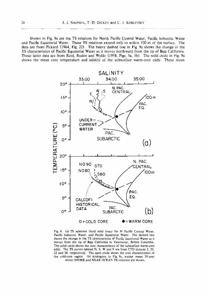
Shown in Fig. 9a are the TS relat ions for Nor th Pacific Centra l Water , Pacific Subarctic Water and Pacific Equatorial Water . These TS relat ions ex t end only to within 100 m of the surface. The data are f rom Pickard (1964, Fig. 22). The heavy dashed line in Fig. 9a shows the change in the TS characteris t ics of Pacific Equatorial Water as it m o v e s nor thward f rom the tip of Baja California. These latter data are f rom Reid, Roden and Wyllie (1958, Figs. 5a, 5b). The solid circle in Fig. 9a shows the m e a n core t em pe r a t u r e and salinity of the subsurface warm-core eddy. These m e a n
A
r..) o
w r'r
r~ W 13.
W N-
20 °
15 o
I0 o
5 °
0 °
SALINITY 33.00 34.00 .'.'55.00
I I i i I l
N. PAC. W ..S CENTRAL
E',~II~',: / / 0 0 m
C##TR##T /
SUBARCTIC ((])
20 ° I I I I 1 I N. PAC.
NO90 S70 / C E N T R A L 15 ° NOBO i $80 / / l O O m
,oo / / /
/ / \ / PAC. 5o I / EQ
CALCOFI ~ ~EQ. HISTORICAL - - - - " " " " ~ X
OO DATA PAC. SUBARCTIC (b)
O=COLD CORE O=WARM CORE
Fig. 9. (a) TS relations (bold solid lines) for N. Pacific Central Water, Pacific Subarctic Water, and Pacific Equatorial Water. The dashed line shows the change in the TS characteristics of Pacific Equatorial Water as it moves from the tip of Baja California to Vancouver, British Columbia. The solid circle shows the core characteristics of the subsurface warm-core eddy. The TS curves labeled N, S, W and E are from CTD stations 2, 20, 22 and 38, respectively. The open circle shows the core characteristics of the cold-core region. (b) Analogous to Fig. 9a, except mean 30-year
winter SHORE and NEAR OCEAN TS relations are shown.

An Offshore California Current Eddy -- I: Interior Dynamics 21
values (T = 7.98°C, S = 34.23) correspond almost exactly to the temperature and salinity of the CU jet off Pt. Conception (see Reid, Roden and Wyllie, 1958). Also shown in Fig, 9a are the indi- vidual TS relations for the upper 300 m of CTD stations 2 (northern), 20 (southern), 22 (western) and 38 (eastern). The open circle in Fig. 9a shows the mean values (T = 10.8°C, S = 33.6) of the central cold-core region. These latter data show that the central cold-core region contains a mixture of both coastal and oceanic waters. Figure 9b is similar to Fig. %, except that mean winter TS rela- tions for the upper 300 m are used instead of upper 300 m data from individual stations sampled during the January 1981 cruise. Only winter data (from Lynn, Bliss and Eber, 1982) were used to calculate these mean TS curves because near-surface TS relations show large variability in structure associated with seasonal changes in the air-sea exchange of heat and moisture (e.g., Emery and O'Brien, 1978). The mean inshore TS relations (labeled $70 and $80 in Fig. 9b) were averaged from data taken at CalCOFI stations 70:53, 70:60, 70:70, 80:52, 80:55 and 80:60. Near-ocean TS relations (labeled N090 and N080 in Fig. 9b) were constructed from data taken at CalCOFI sta- tions 80:120, 80:100, 80:90, 80:80, 90:120, 90:100, 90:90 and 90:80. The locations of these Cal- COFI stations relative to the center of the eddy system are marked with solid squares and solid dia- monds, respectively, in Fig. 1. These historical data also show that the cold-core contains water whose characteristics are associated with a mixture of predominantly coastal water and lesser amounts of near-surface oceanic water.
The salinity fronts shown in Figs. 4, 6 and 7 also provide important information on the sources of water which interact with the eddy system. CalCOFI line 80 passes through the center of the observational area and CalCOFI lines 70 and 90 are near the northern and southern boun- daries of the observation area (see Fig. 1). Thirty-year mean cross-shelf vertical sections of salinity along these CalCOFI lines for the month of January are given by Lynn, Bliss and Eber (1982, pp. 11 and 13). These mean vertical sections show that there is a pronounced near-surface (--0- 100 m) salinity minimum in the offshore CC which extends from about 300 to about 500 km offshore. For January, this salinity minimum is 33.2 or less along lines 70 and 80, while its value is 33.4 or less along line 90. The higher value along line 90 is associated with the mean N-S increas- ing gradient in salinity in the CC (Robinson, 1976). This offshore salinity minimum persists in the CC throughout the year, although it does have a seasonal dependence (see Lynn, Bliss and Eber, 1982). The salinity front which occurs along the southwestern quadrant of the eddy system has salinity values in the range 33.6 to 33.75 over the depth range 0-100 m. Offshore surface waters in the CC with salinities this high generally are found 700 km from shore (Lynn, Bliss and Eber, 1982). These higher salinities are associated with the North Pacific Central water mass. Likewise, the 33.35-33.4 salinity water in the frontal structures along the northeast quadrant of the eddy sys- tem typically occurs within 100 km of shore (Lynn, Bliss and Eber, 1982). These inshore, higher- salinity waters are associated with upwelled waters.
Temperature is the property which most distinguishes the structure of the cold-core from that of the warm-core eddy. Shown in Fig. 10a as bold lines are 30-year mean vertical profiles of tem- perature for January calculated from historical data (Lynn, Bliss and Eber, 1982) along CalCOFI lines 70, 80 and 90. SHORE and NEAR OCEAN mean profiles were constructed from data col- lected at the CalCOFI stations cited above. The OCEAN mean profile was constructed from data taken at CalCOFI stations 90:200 and 90:180. The locations of these stations relative to the center of the eddy are marked with solid triangles in Fig. 1. The extreme FAR-FIELD temperature profiles (e.g., CTD stations 2, 20, 22 and 38 of Fig. 1) also are shown in Fig. 10a. The temperature profiles of CTD stations 2 and 38 (northeastern quadrant of the eddy system) show near-surface structure similar to the mean NEAR OCEAN profile to a depth of about 50-75 m. Below this depth, both stations 2 and 38 show structure similar to the mean SHORE profile. The temperature profiles of CTD stations 20 and 22 (southwestern quadrant) show structure above 50 m similar to the mean OCEAN profile, while below 50 m the temperature structure converges to that of the mean NEAR OCEAN profile.
Salinity profiles, corresponding to the temperature profiles shown in Fig. 10a, are shown in Fig. 10b. To properly interpret these data, it is necessary to know that, while vertical sections of

22 J . J . SIMPSON, T. D. DICKEY and C J. KOBLINSKY
TEMPERATURE (°C)
8 I0 12 14 16 18 I i L i i 1 i i i i J
0 SHORE# 2 | 38 22 20 I
5O
I00
NEAR OCEAN
150 OCEAN
2
200
Is,SHORE/ 20
NEAR k \ 22 OCEAh ~\ I
I00
2
38
50
(b)
150 -
200 ]
OCEAN
Ld rr SALINITY
co 33 O0 33.50 34.00 co Ld 0 I J n," 0._
3450 i
Fig. 10. (a) Thirty-year mean winter profiles of temperature (bold lines) for SHORE, NEAR OCEAN and OCEAN CalCOFI stations. Temperature profiles for CTD stations 2, 20, 22 and 38 also are shown. (b) Analogous
to Fig. 10a, except salinity profiles.
temperature perpendicular to the coast in the CCS show a monotonic increase in temperature with increasing distance from the coast (e.g., see Figs. on p. 5, 57, 90 and 109 of Lynn, Bliss and Eber, 1982), similar sections of salinity show a max imum at the coast, a m i n i m u m in the offshore CCS and then a monotonic increase in salinity with still farther increasing distance from the coast (e.g., see Figs. on p. 13, 65, 117 and 169 of Lynn, Bliss and Eber, 1982). This offshore salinity

An Offshore California Current Eddy -- I: Interior Dynamics 23
minimum results from the presence of waters of Subarctic origin in the offshore CCS and explains why the mean SHORE profile of salinity is saltier than the mean NEAR OCEAN profile. The salinity profiles of CTD stations 20 and 22 (southwestern quadrant) show near-surface structure similar to the mean OCEAN profile of salt, but significantly reduced in salt content compared to the mean OCEAN profile, Below 75 m, these stations show complicated structure which varies between NEAR OCEAN and SHORE mean structure. The salinity profiles of CTD stations 2 and 38 (northeastern quadrant) show near-surface structure which varies between NEAR OCEAN and SHORE mean salinity structure above 75 m. Below 75 m, the salinity structure of CTD station 2 nearly coincides with the mean SHORE salinity structure, while the structure of CTD station 38 approaches the mean SHORE salinity structure.
None of the FAR-FIELD temperature or salinity profiles (Stations 2, 20, 22, 38) shown in Fig. 10a or 10b is exclusively of OCEAN, NEAR OCEAN or SHORE origin. The data in Figs. 10a and 10b suggest that non-linear mixing between surface waters (e.g., 0-200 m) of coastal and oce- anic origin produced these profiles. The chemical analyses of nutrients, dissolved oxygen and chlorophyll a pigment (Simpson, 1984) and biological distributions (Haury, 1984) provide addi- tional evidence in support of these non-linear mixing processes.
The data (Figs. 8, 9, 10), coupled with the geographical distribution of water masses in the CCS (see Section 3), show thai the warm-saline core of the eddy, which is located between 250 and 600 m in depth, consists of inshore water. The combination of high salinity, low dissolved oxygen and warm temperature uniquely identifies this core water mass as California Undercurrent water (Reid, 1965b; Reid, Roden and Wyllie, 1958; Wooster and Jones, 1970). Below 700 m, water from the DPF, as evidenced by the pronounced oxygen minimum near 800 m, is found. The cold-core region has a core water mass composed of a mixture of predominantly freshly upwelled coastal water and lesser amounts of offshore oceanic surface water. The observed distributions of prop- erties are inconsistent with a single, local generation process for the eddy system because no such dynamical process could produce the combined distribution of properties shown in Figs. 2 -- 10. In addition, the subsurface structure may (or may not) be entirely separate in origin From the surface part. The data are insufficient to resolve this point.
The above discussion divided the eddy system into three layers: subsurface warm-core eddy, warm surface layer, and cold-core region. This division was motivated by the observed distribu- tions of water properties. The physical dynamics discussed below and by Koblinsky, Simpson and Dickey (1984), the chemical structure (Simpson, 1984), and the biological distributions (Haury, 1984) also support division of the eddy system into three distinct layers. Based upon water property analysis, one could also identify a fourth quiescent layer below the eddy system. Such a layer, however, is not explicitly discussed in this study because it did not interact physically, chemi- cally or biologically in a significant way with the eddy system.
6. ANOMALY STRUCTURE
The anomalies of heat, salt, and other water properties are important because the magnitude of the anomaly, relative to the surrounding oceanic water, determines the effectiveness of the eddy as an oceanic transporter of heat, salt, or some other property. Several authors (e.g., Newton, 1961; Cheney and Richardson, 1976) have emphasized this potential role of eddies in major oce- anic current systems.
The differential temperature anomaly (°C) is defined by
DTA (r,p) = Te(r, p) - Tfr(p) (1)
where Te(r, p) is the vertical profile of temperature measured at an EDDY station (see Fig. l) some radial distance r from the eddy's center, Tff(p) is the reference vertical profile of temperature con- structed as the arithmetic average of all FAR-FIELD temperature profiles (see Fig. 1), and p is

24 J . J . SIMPSON, T. D. D ICKEY and C. J. KOBLINSKY
pressure. This definition is consistent with the previous usage (Section 5) of the terms EDDY and FAR-FIELD. Radial distributions of DTA along the NS and EW transects of Fig. 1 are shown in Fig. 11. A large positive DTA extends from a depth of about 250 m to about 1400 m. The max- imum in positive DTA occurs in the center of the eddy system at a depth of about 400 m. A region of large negative DTA occurs between 75 and 175 m at the center of the eddy system. This maximum in negative DTA corresponds to the cold-core region shown in Figs. 2, 6a and 7a. The spatial extent of positive DTA associated with the subsurface warm-core eddy greatly exceeds the spatial extent of negative DTA associated with the cold-core region. Between these two major anomaly structures lies a region where the DTA is zero. This latter region, centered near 200 m in the vertical, coincides with the region of minimum vertical shear (Fig. 2) discussed in Section 5. The DTA of the surface layer is very small compared to that of either the subsurface warm-core eddy or the cold-core region. The DTA in the surface layer, however, is consistent with the flow of colder waters from the northeast and warmer waters from the southwest into the surface layer of the eddy system.
DIFFERENTIAL TEMPERATURE ANOMALY (°C) N CONTOUR INTERVAL= O.25 S W E
STA 7 14 28 36 O I I I I I F _ _ J L / I _ _ _ / ~ L L I
CONTOUR INTERVAL =O, I
,ooo
15OO I ~ ~ , , i , , ~ , - I OO t50 200 250 150 200 250 I
Iq EDDY ~1 ~ EDDY I
• DISTANCE(kin) •
Fig. 11. Radial distributions of the differential temperature anomaly (DTA).

An Offshore California Current Eddy -- I: Interior Dynamics 25
The differential salt anomaly (kg kg-1), the differential oxygen anomaly (p.M kg-1), and the differential density anomaly (kg m -3) are defined, in an analogous way to that of DTA, by
DSA(r,p) = Se(r,p) - Sf(p) (2)
DOA(r,p) = Oe(r,p) - Off(p) (3)
and
DMA(r,p) = pe(r,p) - pf(p) ( 4 )
where Se(r,p), Oe(r,p), and pe(r,p) are vertical profiles of salinity, dissolved oxygen and density measured at an EDDY station some radial distance r from the eddy's center, and S~-(p), Off(p) and pf(p) are the corresponding reference profiles of salt, dissolved oxygen and density constructed from the FAR-FIELD stations in a manner exactly analogous to that used to construct Tfr(p). Radial distributions of DSA, DOA and DMA are shown in Figs. 12-14, respectively. The DSA (Fig. 12), unlike the DTA (Fig. 11), has a large positive value in both the subsurface warm-core eddy and in the cold-core region, while the DOA (Fig. 13) has a large negative value in both the subsurface warm-core eddy and in the cold-core region. All three' differential anomaly structures are consistent with the discussion in Section 3 and the results in Section 5. The subsurface warm-
w n ~
w n ~ o_
DIFFERENTIAL SALT ANOMALY xlO (kg.kg -~) N CONTOUR INTERVAL= 0.1
STA 7
5 0 0 . .
000:
s 14
, i ~t '
W E 28 56
1
t 1 5 0 0 , ~ , ~ ~ - - I , , ~ ~ ,
I 0 0 150 2 0 0 2 5 0 I 150 2 0 0 2 5 0 19 EDDY ~,1 I ~ EDDY "'
• D I S T A N C E ( k m ) •
--+
Fig. 12. Radial distributions of the differential salt anomaly (DSA).

26 J . J . SIMPSON, T. D. DICKEY and C. J. KOBLINSKY
core eddy has a core of CU water and hence from Table 1 its DTA should be large and positive, its DSA should be large and positive, but its DOA should be large and negative. The cold-core region, however, contains a mixture of predominantly freshly upwelled coastal water and some offshore oceanic surface water. Hence, from Table 1 its DTA and DOA should be large and nega- tive while its DSA should be large and positive. The change in sign of the DSA below 600 m and in the DOA below 500 m is consistent with the vertical distribution of water properties and vortic- ity dynamics. This is shown explicitly in Section 9.
The DMA (Fig. 14) shows structure exactly like that of DTA (Fig. 11). There is a large mass deficit associated with the subsurface warm-core eddy and a large mass excess associated with the cold-core region which lies above it. Between these two regions of density anomaly, there is a much smaller, nearly uniform zone of zero density anomaly. This zone occurs between 200-250 m. The 26.4 isopycnal (Fig. 3) defines the center of this zone. The distribution of DMA shown in Fig. 14 suggests that exchange of water between the threeqayer system and the FAR-FIELD may have occurred near the 26.4 isopycnal. The density anomaly structure shown in Fig. 14 also shows that both the core of the subsurface warm-core eddy (--250-600 m) and the central cold-core region consist of non-local waters.
Most other studies of mesoscale rings and eddies (e.g., Elliot, 1979; Joyce, Patterson and Millard, 1981) have calculated the integrated anomaly structure per unit area of a ring or eddy, rather than its differential anomaly. A generalized equation to calculate the integrated anomaly structure per unit area of some water property qJ is given by
n o
( /3 U ) L d r Y
N STA
0
500
1000
1500 I00
DIFFERENTIAL OXYGEN ANOMALY xlO (/~M.kg -I)
CONTOUR INTERVAL=0.4 S W E 14 28 56
_ _ I I ~ I I ~ ~ i r_ i I _ _ _ _ L _ I I I i
; ~ i
' i !
4
0 i
_ J L _ _ J i i i i i i
150 200 250 I 150 200 EDDY ~ I I_u EDDY
• DrSTANCE(km) •
2501
Fig. 13. Radial distributions oflhedifferential oxygen anomaly (DOA).

An Offshore California Current Eddy - "I: Interior Dynamics 27
I toA( r ,p ) = k+ ,~ [toe(r,p ') - to t r (P ' ) ldp ' p~
(5)
where g,e(r,p') is the vertical profile of to measured at an E D D Y station s o m e radial distance r from the center of the eddy, tofr(P') is the FAR-FIELD reference profile for property tO, kq, is a constant associated with property to, Pr is a reference pressure for the integration, and p' is a d u m m y variable of integration. If to were temperature, then Eq. (5) could be used to calculate the heat content anomaly per unit area
IHA(r,p) = c~---2-, j~ [Te(r,p') - Tff(p')]dp' (6) g p~
w rY
(/)
o~ w OE (I_
DIFFERENTIAL N CONTOUR INTERVAL=0.5 S
ST,&, 7 14 0 1 ~ i , ~ . . _ l _ _ J ~ I L
L
Ioo
,5o ! - - 0 ~ / / , " ( ~ - ~ ' f l \ \ \ ' % X \
2 5 0 i ] i i i
DENSITY ANOMALY xlO (kg.m-3) w E 28 36
I [ _ _ L ] _ _ . I I I I ~___
CONTOURINTERVAL=0.2
!
~°° i --I 6
i r I000 !
i
15oo -~ - IOO
* -
4
i i i i i i ~ ~ i i
150 200 250 150 200 250 EDDY ~,1 4 EDDY ,--
• DI STANCE (km) •
Fig. 14. Radial distributions of the differential density anomaly (DMA).
28 J .J . S I M P S O N , T. D. DICKEY and C. J. KOBLINSKY
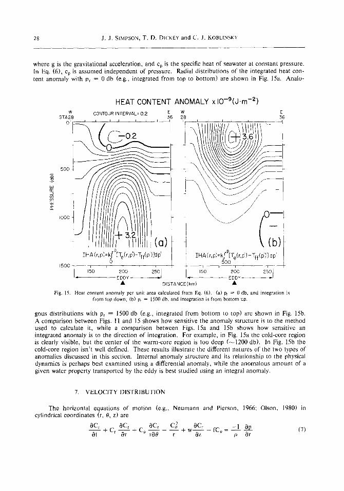
where g is the gravitational acceleration, and cp is the specific heat of seawater at constant pressure. In Eq. (6), % is assumed independent of pressure. Radial distributions of the integrated heat con- tent anomaly with Pr = 0 db (e.g., integrated from top to bottom) are shown in Fig. 15a. Analo-
w Pc"
w
o_
W S T A 2 8
O'
500
i 0 0 0
HEAT CONTENT ANOMALY x 10-9(J.m -z) CONTOUR INTERVAL= 0.2 E W E
36 28 36
13 i r i
]:HA(r,p)= kf [Te(r,p)-Tff(p)] d p 1500 ~_ 1500
I I i i
I ,5o 2oo 25o I I ,5o 2oo ~' EDDY ~ q EDDY '~
• DISTANCE(km) •
Fig. 15. Heat content anomaly per unit area calculated from Eq. (6). (a) p~ = 0 db, and integration is from top down; (b) p, = 1500 db, and integration is from bottom up.
gous distributions with Pr = 1500 db (e.g., integrated from bottom to top) are shown in Fig. 15b. A comparison between Figs. 11 and 15 shows how sensitive the anomaly structure is to the method used to calculate it, while a comparison between Figs. 15a and 15b shows how sensitive an integrated anomaly is to the direction of integration. For example, in Fig. 15a the cold-core region is clearly visible, but the center of the warm-core region is too deep (--1200 db). In Fig. 15b the cold-core region isn't well defined. These results illustrate the different natures of the two types of anomalies discussed in this section. Internal anomaly structure and its relationship to the physical dynamics is perhaps best examined using a differential anomaly, while the anomalous amount of a given water property transported by the eddy is best studied using an integral anomaly.
7. VELOCITY DISTRIBUTION
The horizontal equations of motion (e.g., Neumann and Pierson, 1966; OIson, 1980) in cylindrical coordinates (r, 0, z) are
OCr aCr °qCr C2 4- Oqcr - 1 . ~ O"-"~ -f- Cr ~ -{'- C0 raO r W~z fC. = - - (7) p 8r

An Offshore California Current Eddy -- I: Interior Dynamics 29
(3C° (3C° (3C° CrC° w (3Co - 1 (3p (3--t + C r ~ + C ° ~ + r + ~ + f C r = - - O r(30 (8)
where Cr = dr/dt is the radial velocity; Co = rd0/dt is the tangential (or azimuthal) velocity; w is the vertical velocity; p is pressure; p is density; f is the Coriolis parameter; and t is time. Cylindri- cal coordinates are used because of the symmetry in the data. Data collection took nine days. Hence, viscous terms are neglected in this analysis because on short time scales (--several weeks) they appear to be negligible (Olson, 1980). The lack of a sufficient number of synoptic radial sec- tions through the system precludes the construction of a meaningful plan view of any water pro- perty. Hence, we assumed that the velocity distribution has circular symmetry (e.g., (3Cr/(30 = (3C0/(30 = 0). This assumption, however, is partially justified by the circular symmetry seen in the patterns of surface brightness temperature directly above the eddy system (see Koblinsky, Simpson and Dickey, 1984, Fig. 1). If the motion is also stationary (e.g., (3Cr/0t = (3C0/(3t = 0), follows curved isobars whose centers are at r = 0 (e.g., (3p/(30 = 0), and the vertical and radial velocities are negligible (e.g., Cr = w -- 0), then Eq. (8) is satisfied identi- cally and Eq. (7) reduces to
C°2 + f C o - 1 Op = 0 (9) r p (3r
where the radial pressure gradient in Eq. (9) is related to the magnitude of the geostrophic velocity,
Vg, through the equation Vg= o-~-[-~rr[. Thus, for normal anticyclonic flow about a high (e.g.,
(3p/(3r < 0), the centrifugal force augments the horizontal pressure gradient force, and the gradient (i.e. azimuthal) speed is enhanced. The solution to Eq. (9) for normal anticyclonic flow is
Co = T + + - - (10) p Or
Equation (10) satisfies the dynamical constraint that Co ~ 0 as (3p/(3r ~ 0. When (3p/(3r < 0 (a high), the square root in Eq. (10) is smaller in magnitude than fr/2 and Co is negative (anti- cyclonic). Thus, the sign convention used in Eqs. (7)-(10) is consistent with that of standard polar coordinates. Further, it is shown in Section 9 that the assumption Cr = 0 is justified on indepen- dent dynamical grounds, because the alternate assumption (Cr ~ 0) imposes a severe and unrealistic dynamical constraint on the absolute vorticity. A more complete discussion of both nor- mal and anomalous gradient flow is given by Hess (1959).
Geostrophic velocities were calculated by vertically integrating (relative to 1450 db) profiles of the specific volume anomaly which were determined from density. Geostrophic velocities were obtained from these integrals by finite differencing between pairs of stations. This calculation assumes hydrostatic balance in the vertical
1 ~ = - g (11) O (3z
There are several sources of errors in the geostrophic calculations. Of these, the choice of reference level (1450 db) and navigational errors are the most important. Navigational errors can affect the geostrophic velocity significantly because the station separation used in the calculation is determined from the navigation. Loran C (accuracy _+ 1 to 2 kin) was used during this experiment.
30 J . J . SIMPSON, T. D. DICKEY and C. J. KOBI.INSKY
Olson (1980) used similar navigational equipment and conservatively estimated errors in the geo- strophic velocity, which result from errors in center determination and station spacing, to be 10%. Geostrophic calculations were performed with other reference levels between 1000 and 1450 db. No change in velocity structure resulted: only the magnitude changed slightly (--0.01 m s I). Such small changes are insignificant to this work. These changes were small because the shear structure between 1000 and 1450 m is small. These results confirm the validity of our choice of reference level. Observational errors in the relative field of pressure are typically 5% (e.g., Emery, 1975). Hence, we estimate that the errors associated with the geostrophic velocities reported in this paper are at most 15%.
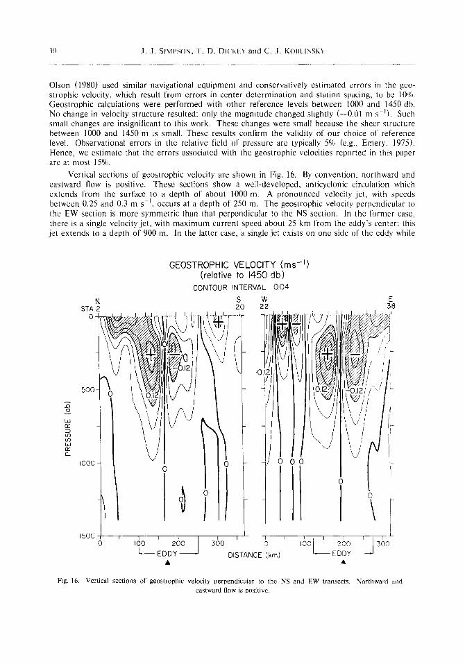
Vertical sections of geostrophic velocity are shown in Fig. 16. By convention, northward and eastward flow is positive. These sections show a well-developed, anticyclonic circulation which extends from the surface to a depth of about 1000 m. A pronounced velocity jet, with speeds between 0.25 and 0.3 m s -1, occurs at a depth of 250 m. The geostrophic velocity perpendicular to the EW section is more symmetric than that perpendicular to the NS section. In the former case, there is a single velocity jet, with maximum current speed about 25 km from the eddy's center: this jet extends to a depth of 900 m. In the latter case, a single jet exists on one side of the eddy while
W n~
D
W n ~ 12.
N STA 2
i
0
GEOSTROPHIC VELOCITY (ms - j ) (relative to 1450 db)
CONTOUR INTERVAL 004
S w 20 22
o o
E 38
I I
jf: o
o
f
,8o ' ,oo 200 . 300 o 2#o
[. EDDY DISTANCE (km) EDDY
Fig. 16. Vertical sections of geostrophic velocity perpendicular to the NS and EW transects. Northward and eastward flow is positive.
An Offshore California Current Eddy -- I: Interior Dynamics 31
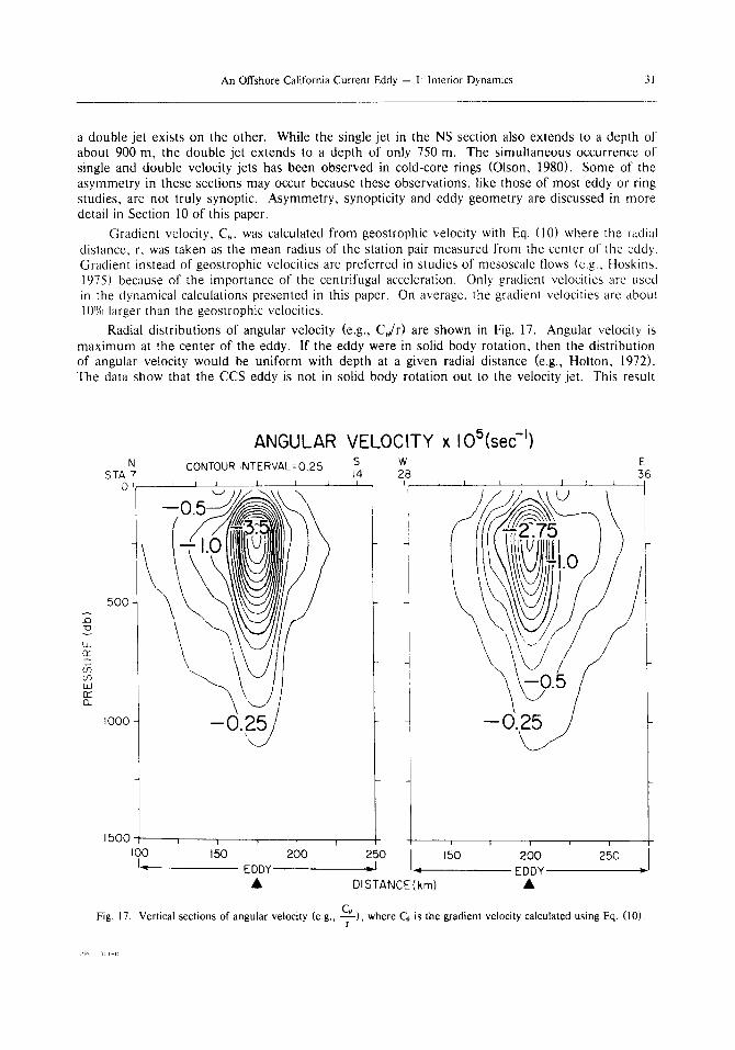
a double jet exists on the other. While the single jet in the NS section also extends to a depth of about 900 m, the double jet extends to a depth of only 750 m. The simultaneous occurrence of single and double velocity jets has been observed in cold-core rings (Olson, 1980). Some of the asymmetry in these sections may occur because these observations, like those of most eddy or ring studies, are not truly synoptic. Asymmetry, synopticity and eddy geometry are discussed in more detail in Section 10 of this paper.
Gradient velocity, Co, was calculated from geostrophic velocity with Eq. (10) where the radial distance, r, was taken as the mean radius of the station pair measured from the center of" the eddy. Gradient instead of geostrophic velocities are preferred in studies of mesoscale flows (e.g., Hoskins, 1975) because of the importance of the centrifugal acceleration. Only gradient velocities are used in the dynamical calculations presented in this paper. On average, the gradient velocities are about 10% larger than the geostrophic velocities.
Radial distributions of angular velocity (e.g., C0/r) are shown in Fig. 17. Angular velocity is maximum at the center of the eddy. If the eddy were in solid body rotation, then the distribution of angular velocity would be uniform with depth at a given radial distance (e.g., Holton, 1972). The data show that the CCS eddy is not in solid body rotation out to the velocity jet. This result
N
STA 7 0
500
I 0 0 0 -
ANGULAR VELOCITY x IOS(sec H) CONTOUR INTERVAL= 0.25 S
14 I i ~ I I I I
w 28 1 I i i i i i i
:Jl cs 7 -0.
i E
E 36
1500 I I I I i i i l i
IO0 150 200 250 150 200 250 I-- EDDY -_1 q EDDY
A DISTANCE(km) •
Fig. 17. Vertical sections of angular velocity (e.g., CO), where Co is the gradient velocity calculated using Eq. (10). r

32 J . J . SIMPSON, T. D. DICKEY and C. J. KOBLINSKY
differs sharply from that reported by Olson (1980) who showed that out to a radius of - -40 km ring BOB was in near solid body rotation. Olson (1980), however, did not show radial distributions of angular velocity. Instead, he plotted the normalized radial distribution of normalized gradient velocity at a given depth.
The differences in velocity structure between the CCS eddy and ring BOB can be interpreted in terms of the theoretically expected velocity distribution induced by a single, circular vortex of radius a and strength K. The velocity distribution induced by such a vortex is that of a solid body for r ~ a, while for r > a the flow is irrotational and the velocity decays as k]/r (Milne-Thomson, 1968). The constant k] is dependent upon the geometry and strength of the vortex. In Fig. 18a,
1.0
0.5
co o - - 0
COMA'X 1.0
0.5
NORMALIZED GRADIENT VELOCITY (rel(]tive to 1450 db)
0 0
~, jeli~p,k" -.. 0- - - - -0 N-C a j / o o _c , ,
. .~. .
i L ~ ........... 1.0 2.0 3.0 410
-t I,,,,~'~ f . ~ " ~ MEAN SIMPSON, DICKEY, 1 I / A~" / ',\ ~,rn KOBLINSKY, (1984)
~ ' ~ " /?" / ~ \ . . ~ GAUSSIAN , ¢ / -., SOL,D BODY n / / " \ \ ~ 7XPONENTIAL DECAY
/ / / ~ .. \ ~ POTENTIAL FLOW / / / ' , \ . \ \ 1/ / .\ ' ~ \ a [] MEAN DATA
/ / / , X. o
D ~ / \
J I L d
1.0 2.0 3.0 4.0
r/r MAX
Fig. 18. (a) Radial distributions of normalized gradient velocity as a function of normalized radial distance from the center of the eddy. Data are shown with symbols. (b) Mean of the four distributions shown in (a),
and other velocity distributions as indicated in figure key.

33 An Offshore California Current Eddy -- I: Interior Dynamics
four normalized radial distributions of normalized gradient velocity (with data) are shown. The data are from the 250 m level. This depth corresponds to the depth of maximum gradient velocity. The normalization factors used for each of the curves shown in Fig. 18a were the maximum gra- dient velocity COMAX along that radius and the radial distance r = FMA x at which Co = COMAX.
Shown in Fig. 18b are: the mean of the four distributions shown in Fig. 18a, the velocity distribu- tion for the solid body rotation of a circular vortex for r ~< a, the velocity distribution associated with the potential flow of a circular vortex for r > a, the exponential decay function u =
u0.exp(c~(1- r )) used by Olson (1980) to fit data from cold-core ring BOB, and the normalized FMAX
velocity distribution of a Gaussian eddy. An eddy is said to be Gaussian if its radial height field is Gaussian (e.g,, p(r,z) = f(z)exp(-r2/2)) (see Smith and Reid, 1982). Such an eddy has an azimu- thal velocity C o ¢c 0p/e3r and a value of Co = 0 at r = 0. Its value of C,/r, however, is maximum at r = 0. The data in Figs. 17 and 18 support neither solid body rotation of the CCS eddy out to the velocity jet nor exponential decay of the gradient velocity beyond the velocity jet. For a nor- malized radial distance of r/rMA x >/ 2.5, the data are consistent with the kl/r decay of the potential flow induced by a circular vortex of radius a.
The magnitude of the radial gradient of angular velocity (see Fig. 17) is small close to the eddy center compared to the magnitude of this quantity near the velocity jet. One could interpret this as evidence for a small region of near solid body rotation very close to the eddy center. The spatial resolution of the CTD survey, however, is too coarse to adequately resolve this point. The radial derivative of the velocity distribution induced by a circular vortex has a discontinuity at r = a (Fig. 18b). No such discontinuity is shown in the radial derivative of the measured velocity distri- bution (Fig. 18b). Rather, there is a broad transition regime between what might be interpreted as a very small region of solid body rotation immediately adjacent to r = 0 and the potential flow regime at r > > a. This transition region dominates the measured radial distribution of Co and is approximately Gaussian in shape. Hence, our observations of gradient velocity, unlike those of Olson (1980), support the use of a Gaussian radial height field as an initial condition in models (e.g., Bretherton and Karweit, 1975; Mied and Lindemann, 1979; McWilliams and Flierl, 1979; Smith and Reid, 1982) of oceanic eddies. The difference between the observed radial distribution of C~ and that induced by a circular vortex may be due to viscous effects which are ignored in the theory of isolated, circular vortices (see Milne-Thomson, 1968). While viscous effects can be ignored on the time scales associated with this study (--10 days), their effects cannot be ignored over the lifetime of an eddy (many months to years).
8. ENERGETICS
The energy per unit area of a column of water consists of a baroclinic and a barotropic com- ponent. The baroclinic component occurs because isopycnal surfaces generally are not parallel to geopotential surfaces. The baroclinic component is estimated reasonably well from CTD observa- tions. The barotropic component is much more difficult to determine because the absolute field of mass must be known. Hence, an accurate bottom pressure measurement, in addition to the CTD observations, is required. This section deals only with the baroclinic component of energy.
The baroclinic component of energy itself consists of two parts: the baroclinic kinetic energy and the baroclinic potential energy. The baroclinic kinetic energy per unit area, KE(r,p), is obtained by vertically integrating the squared gradient velocities which were calculated with Eq. (10).
KE(r,p) ~_g ) 2 , , = Co (r ,p )dp Pr
(12)

34 J . J . SIMPSON, T. D. DICKEY and C. J. KOBI.INSKY
where Pr is a reference pressure for the integration (taken here as pr = 1000 db), g is the gravita- tional acceleration, and p' is a dummy variable of integration. The total baroclinic kinetic energy, TKE, is obtained by integrating Eq. (12) over the surface area of the eddy. This integration assumes that the kinetic energy per unit area is known as a continuous function of radial distance r. The kinetic energy per unit area, however, generally is not known as a continuous function of radial distance. Rather, it is known only at discrete radial distances from the center of the eddy. These distances correspond to the locations midway between adjacent CTD casts. Nonetheless, a good approximation to TKE is obtained by integration over individual annular regions of the eddy under the assumption that the distribution of KE(r,p) within a given annular region is accurately given by the mean value of KE{77~ obtained from the measured endpoint values which define the annular region. A given realization of TKE for the eddy is obtained by summing over all annular regions along a given radius. A better approximation of TKE is obtained by repeating this pro- cedure along all measured radii because any azimuthal variation in the distribution of KE(r,p) will be incorporated into the ensemble average of TKE. A more detailed discussion of the procedure is given by Elliot (1979).
Lorenz (1955) showed that the total baroclinic potential energy consists of two components. That part available for conversion to eddy kinetic energy is called the available potential energy (APE). The other part is associated with a horizontally uniform density stratification, is unavailable for conversion to eddy kinetic energy, and is called the unavailable potential energy (UPE). Most reported calculations of available potential energy for isolated rings (e.g., Barrett, 1971; Cheney and Richardson, 1976) were made from CTD observations using Fofonoff's (1962) integrated gravita- tional potential energy anomaly. Such estimates represent the purely gravitational component of available potential energy, APEg. Reid, Elliot and Olson (1981) have shown, however, that such an approximation to APE can seriously overestimate the baroclinic potential energy available for conversion to baroclinic kinetic energy because it ignores the elastic internal energy component of APE (e.g., APE i) and because estimates of APEg are very sensitive to errors in the choice of refer- ence state. To first order, the corrected expression for the APE per unit area is
pr [ Pr(P)g I dp' (13)
where N2(p ') is the squared Brunt-V~isgil~i frequency of the reference state, #r(P') is the density dis- tribution of the reference state, kP(r ,p ' ) is the pressure displacement for a given material surface between the perturbation and reference states, g is the gravitational acceleration, Pr is the reference pressure (here Pr = 1000 db) and p' is a dummy variable of integration. Eq. (13) is the first term in the series expansion of the Margules-Lorenz (ML) definition of APE (see Reid, Elliot and Olson, 1981, Eq. 36). They also have shown that Eq. (13) is equivalent to the Boussinesq approxi- mation to APE used by Olson (1980) and by Joyce, Patterson and Millard (1981) where the vertical displacement of a given material surface, 8, is related to the AP in Eq. (13) by AP = -tJrg& For this calculation, the reference profile was defined as the average of all measured profiles labeled FAR-FIELD in Fig. 1. This definition is consistent with previous usage in Section 5 of this paper. Reid, Elliot and Olson (1981) have shown that use of the first-order term only to calculate APE typically results in an error of order 5% for AP of order 103. Our kP ' s generally are less than order 102. Thus, the error introduced by the use of Eq. (13) should be less than 5%. This error is well within the experimental uncertainties of the data and of the navigation. Eq. (13) (Elliott, 1979; Reid, Elliot and Olson, 1981) defines APE as the maximum kinetic energy that a stably stratified column of water can have if it converts its potential energy to kinetic energy by a process that con- serves entropy. Hence, Eq. (13) requires that the pressure displacement be evaluated between isentropic surfaces. In practice, however, the isentropic surfaces are approximated by surfaces of constant potential density (Elliott, 1979: Olson, 1980). A discussion of the error introduced by the

An Offshore California Current Eddy - I: Interior Dynamics 35
use of density surfaces rather than isentropic surfaces to evaluate Eq. (13), as well as other errors associated with the calculation of APE, is given by Elliott {1979) and by Reid, Elliot and Olson (1981). The total available potential energy (TAPE) then is obtained by integration of Eq. (13) in a manner analogous to that discussed above for TKE.
Radial distributions of the kinetic energy per unit area, calculated with Eq. (12), are shown in Fig. 19. Maximum kinetic energy occurs in the regions of the velocity jets which are located about
N STA
o ,, ~15J
t 500 J
(35
CO ub
cc i Ck
t©o0 1
J
S W 14 28
q l - l I _ _ & : ~
I
CONTOUR INTERVAL= I
--14
0 I
/ 1500 t - ~ , -
I00 150 I,,
2OO E DDY
KINETIC ENERGY xlO-3(J-m -2)
250 ,~1
t
DISTANCE(km)
E Z6
150 200 250
E DDY
Fig. 19. Vertical sections of kinetic energy per unit area, calculated usingEq. (12).
30 km from the center of the eddy. These distributions are radially symmetric about the vertical axis of rotation of the eddy. Radial distributions of the available potential energy per unit area, cal- culated with Eq. (13), are shown in Fig. 20. The integration was limited to the upper 1000 db of the water column to aid comparison with other published estimates of APE. The maximum in the APE occurs at the center of the eddy. The maximum displacement of density surfaces relative to the reference state occurs here and the APE is proportional to the integrated value of this displace- ment squared. APE decreases rapidly with radial distance from the center of the eddy. Qualita- tively, both the distributions of KE and APE reported here are similar to those reported by Joyce, Patterson and Millard (1981) for a cold-core ring observed in the Antarctic Circumpolar Current. It should be noted, however, that while we integrated from 1000 db to the surface for our distribu- tion of APE, Joyce, Patterson and Millard (1981) integrated from the 27.0 to 27.7 density surfaces

36 J . J . SIMPSON, T. D. DICKEY and C. J. KOBLINSKY
n o v
W n~
w n ~ o_
AVAILABLE POTENTIAL ENERGY xlO-3(d'm -z) N CONTOUR INTERVAL= IO S W E
STA 7 , , ~ 1 7 0 , I I 1,4 2 ' ~ 2 5 0 7 m T m l r r F m t ~ , F ~4 , , 56 0
! V
I000
i
J
1 5 0 0 T i i I T - - I i , i i ,
I00 150 200 250 / 150 200 250 I,,, EDDY ,,3 ~, EDDY - -
!
I
DISTANCE(km) I J
Fig. 20. Vertical sections of APE per unit area, calculated using Eq. (13).
(e.g., approximately from 76 to 1393 db).
Inspection of Figs. 19 and 20 also shows how sensitive the calculation of the TAPE/TKE ratio is to the depth of integration and to the radial distance over which the surface integration is done. Hence, intercomparison among TAPE/TKE ratios for different ring or eddy systems must be done with caution. This is especially important when comparing TAPE/TKE ratios between warm- and cold-core eddies or rings because, frequently, cold-core rings are geometrically larger than their warm-core counterparts. For example, the isopycnal displacements of ring BOB occur at least from 100-2000 db and the gradient velocity varies from 1.5 to 0.2 m s -1 (see Figs. 1 and 3, Olson, 1980). Likewise, the cyclonic ring observed in the Drake Passage by Joyce, Patterson and Millard (1981) has isopycnal displacements from 0-3000 db and the geostrophic velocity varied from 0.5 to 0.1 m s -1 over the pressure range 0-2000 db (see Fig. 10, Joyce, Patterson and Millard, 1981). The isopycnal displacements of this CCS eddy (Fig. 3), however, are very small below 1200 db com- pared to those of either ring BOB or the Drake Passage ring, while the maximum gradient velocity (Fig. 16) is only about 0.3 m s - l and it has a near-zero value at 1000 db. With a radius of 50 km and a depth of 500 m, the TAPE/TKE ratio for this CCS eddy is 2.0. This value, however, is uncorrected for the presence of a cold-core region. When the TAPE associated with the cold-core region is subtracted from the TAPE of the system, the TAPE/TKE ratio is 1.9. Hence, only about 5% of the APE of the system is directly associated with the cold-core region. Ratios of TAPE/TKE

An Offshore California Current Eddy -- I: Interior Dynamics 37
for cold-core rings generally range between 1.5 and 3 (e.g., Olson, 1980; Reid, Elliot and Olson, 1981; Joyce, Patterson and Millard, 1981).
The cold-core region does not seriously diminish the value of TAPE because the pressure dis- placements AP in the cold-core region are small compared to corresponding displacements in the warm-core eddy. The presence of the cold-core region, however, affects the calculation of the geo- strophic, and hence gradient, velocities differently. Here, the specific volume anomaly changes sign and the geostrophic velocity decreases from its maximum value in the warm-core eddy as the depth integration proceeds through the cold-core region. Thus, the kinetic energy of the three-layer sys- tem is less than that of an equivalent two-layer system consisting of a warm-core eddy which extends to the base of the surface layer.
9. VORTICITY DISTRIBUTION
The equation for conservation of vorticity is obtained by taking the curl of the momentum equations. In most geophysical applications, the potential vorticity is more useful than the vector vorticity. The potential vorticity can be obtained by taking the scalar product of the vector vorticity with the gradient of the potential density (Pedlosky, 1971).
°II ] o_T XOw o ol IO r Ow r 00 ~zz J+ T, ,~ [ Uzz 0r
(14)
+ "-'~--+ Or r 00 I - f = 0
Eq. (14) is valid for incompressible, inviscid, baroclinic flow. The quantity inside the brackets of Eq. (14) is the potential vorticity perpendicular to the isopycnal surfaces. The potential vorticity may be interpreted physically as a measure of the ratio of the sum of the relative (~) and planetary (f) vorticity to the effective depth of the vortex (Holton, 1972). The spatial derivatives in potential density modulate the absolute vorticity in Eq. (14) and provide an effective depth of
vortex length scale analogous to h in the simpler barotropic case (e.g., 1 3 ( ~ + f ) = 0) For a sym- Dt h "
metric eddy, the vertical density gradient is particularly important. The inviscid assumption res- tricts the use of Eq. (14) to time scales less than one month and horizontal length scales greater than several kilometers.
The relative importance of individual terms in Eq. (14) was determined by scaling the obser- vations in a manner analogous to that presented by Olson (1980). Data at a pressure of 250 db and 30 km from the center of the eddy were used. These data are from the subsurface velocity jet of the eddy. Terms involving radial, azimuthal or vertical derivatives of density or velocity were determined by finite differencing the station data. Cubic splines were used when necessary (e.g.,
terms like 00 {3C0 0r 0z ) to spatially align the finite differences within the numerical grid used to define
the eddy. The radial velocity, Cr, was estimated to be negligible compared to Co, based on Cal- COFI data for the month of January and on the requirement that, for steady curved, isobaric, inviscid flow (e.g., Eq. (9)), C r = 0. C r was not evaluated directly from eddy data. Olson (1980) also took Cr = 0. An independent dynamical constraint, which strongly supports the assumption Cr = 0, follows directly from Eq. (8) if all the constraints placed on Eqs. (7) and (8) in Section 7 are retained, except now it is assumed Cr ;~ 0. Then, instead of being satisfied identically, Eq. (8)

38 J.J. SIMPSON, T. D. DICKEY and C. J. KOBLINSKY
becomes
Co OC0 - - + f (15)
r Or
The relative vorticity ~ = C0/r + 3C0/Or. Thus, if Cr ;e 0 and the motion is constrained to be sta- tionary, circularly symmetric with curved isobars whose centers are at r = 0, then it follows that the absolute vorticity of the system about the vertical must be zero following a particle (e.g., AV =
+ f = 0). Hess (1959) states that this is a very special case which rarely occurs in nature and that it should be rejected in favor of the assumption Cr = 0. The hydrostatic balance (Eq. (11)) and the results of Olson (1980) justify the neglect of terms involving the vertical velocity, w. The distributions of radial density gradient (Op/Or) and of azimuthal density gradient (Op/O0), although not shown here, were calculated. These gradients are several orders of magnitude smaller than the vertical density gradient (8p/Oz). For this reason, terms in Eq. (14) which contain either 3p/Or or Op/OO are much smaller than terms which contain Op/8z. The terms in Eq. (14) were evaluated along each of the four radii sampled. The mean of these four numbers was taken as the estimate of the term. A direct long-term estimate of the temporal variation in each of the terms in Eq. (14) was not possible because only one cruise was made. It took approximately nine days to complete the survey. Therefore, we interpret the standard deviation about the mean of a given term as an approximate measure of the temporal variability associated with that term over the nine-day period of the cruise. A summary of all estimates is given in Table 2.
TABLE 2. Estimates of the individual terms o1" the vorticity balance. Terms involving w and C~ are assumed Io be
insignificant.
D [ ~ r _ r [ ~ z l ~ z - z [ ~ - 0 G , 0 C r + q l 0 = ~ - - + + Or r 00
Term Unit Value Variation
I ~2_ kg m 4 0.0 + 5.1 X 10 7 r 00
kg m "-4 0.3 X l f f ~ +_ 0.5 X IC c~ Or
0C, s t 6 .3X lO t + 7 .5X lCcS clz
s i 0.25 X 10 5 + 037 X 10
1" s -l 7.9 X 10 5 + 0.2 X 10
~2_ k g m 4 0,9 X IO 2 + 0.5 X 10 Oz
C~ s t 0 . 8 4 X lOS + 0 1 9 X 10⁵ r
c~G, s i 0.51 X 19 ~ + 0.58 X ll) Or

An Offshore California Current Eddy -- I: Interior Dynamics 39
Based on the above results, the first order approximation to the equation for potential vorticity (Eq. (14)) is
0-7 -#F+F = 0 (16)
Eq. (16) was used by Olson (1980) and by Joyce, Patterson and Millard (1981) to study the dynam- ics of cold-core rings in the Gulf Stream and Antarctic Circumpolar Current, respectively. Most of the adjustment seen in these studies of cold-core rings involved the vertical stratification 0p/0z, the radial shear 0C0/0r and the curvature term, CJr. Our results generally are consistent with these other studies. A major difference, however, is the importance of the planetary vorticity compared to the relative vorticity in the vorticity balance for the CCS eddy. Here, the planetary vorticity is about an order of magnitude greater than the relative vorticity.
The vertical component of relative vorticity ¢ = (t#~ + 0C~) r T ' drawn along the transects of
Fig. 1, is shown in Fig. 2l. Relative vorticity within the eddy consists of a region of negative vor-
RELATIVE VORTICITY xlOS(s -') N CONTOUR INTERVAL= 0.25 S W
ST~ 7 14 28
I ~ 500 ~[/
LLI if -D
f U", LL] i' 0:5 CL
I000
9.1
J 1500
I00 I=
, r , , • 4 mO 200 250 I 150
EDDY pl
• DISTANCE(km)
1 i
20O
EDDY
_ oc. Fig. 21. Radial distributions of the vertical component of relative vorticitv [ ~- G, +
" r D r
i
E 36
l
250

4{) J . J . SIMPSON, T. D. DICKEY and C. J. KOBLINSKY
ticity whose maximum occurs at the center of the eddy. Beyond the velocity jet of the eddy, regions of positive relative vorticity are found. The distribution of relative vorticity shows a high degree of axial symmetry about the center of the eddy. There is, however, a noticeable intensification in relative vorticity along the EW section compared to the NS section• This intensification is discussed further in Section 10 of this paper.
In Fig. 22a, normalized relative vorticity (~/~MAX) is shown as a function of normalized radial distance from the eddy's center for the four radii sampled. The normalization procedures are simi- lar to those used to normalize the gradient velocity in Section 7 of this paper. In Fig. 22b, the graphical average of these data and similar data for ring BOB (Olson, 1980) are shown. The distributions of relative vorticity shown in Figs. 21 and 22 are consistent with the expected vorticity distribution of a Gaussian eddy.
N O R M A L I Z E D R E L A T I V E V O R T I C I T Y
1.0
0.5
0.0
- - N--C X%. ~ - - W-C
.... \ ...... E - c ~:,,~ .... \ - - - s - c
' \ \X \%•
\ " \ ~... ~"......~.
(o) C mQX
1.0 ~----~,~ .,'"-\ .... OLSON RING BOB I ~ / / / "~ - - CCS EDDY MEAN
/
I
0.5 L . . . . . . . . . . . . . ..~.// i!
oo ib) i 1
0 2O 40 6O 80 r (km)
Fig. 22. (a) Radial distributions of the normalized relative vorticity as a func- tion of normalized radial distance from the center of the eddy. (b) Mean of the four distributions shown in (a), and the observed distribution from Gulf
Stream ring BOB.

An Offshore California Current Eddy -- l: Interior Dynamics 41
The differential salt and oxygen anomalies (Figs. 12 and 13) change sign below about 700 db. The differential temperature and potential density anomalies (Figs. 11 and 14), however, do not change sign below 700 db. This difference in anomaly structure is a direct result of the combina- tion of the local vertical distributions of water properties below 700 db (see Sections 3 and 5) and the vorticity dynamics of the eddy system. In order for the local waters of the DPF (p > 700 db) to accommodate the non-local subsurface eddy core, the local waters must undergo vortex compression and acquire anticyclonic rotation. The distributions of geostrophic velocity (Fig. 16) show that only the local waters of the DPF directly below the subsurface warm-core eddy acquired the necessary anticyclonic rotation. Moreover, the process of vortex readjustment simul- taneously produces a downward displacement of local isotherms, isohalines, oxypleths and iso- pycnals below about 700 db (e.g, see Figs. 2-5). The net effect of these processes on the differential anomaly structures below 700 m is that shown in Figs. 11-14.
The first order approximation for the potential vorticity (PV) was calculated as the quantity inside the brackets of Eq. (16). PV should be conserved by a parcel of fluid as it circulates around the eddy. Hence, the orientation of isopleths of potential vorticity relative to isopycnals indicates where mixing of EDDY and FAR-FIELD waters may have occurred in the past. Specifically, radial movement along isopycnal surfaces may have occurred everywhere that the isopleths of PV are parallel to isopycnals. If the isopleths of PV intersect the isopycnals obliquely, then exchange was inhibited. If the isopleths of PV and the isopycnals are orthogonal, then no exchange occurred. Vertical sections of PV (solid lines) and of isopycnals (dashed lines) are shown in Fig. 23. Above
qD v
LLI OC
Lr) (J9 B J O:"
O_
POTENTIAL VORTICITY xlO s (kg 'm-4s - t ) N S
STA 7 14
- - = - - , - , , - -7 z ~ _ _ - . . . , . ~
5 0 0 q ~ ~ ~ . . . . . . . . . _ ~ ~
| ~ _ - - ~ ~ / - - / - 2 ~ - / 0 I""----... o 7 0 " " -
,ooo > f
I
1500 1 Ioo
I . .
w 28
'1 t
E 36
k i I 1 I I 1
= 2 5 . 0 ~ - o e . ' ~ - 4 ~ ~ ~ -
- -=- ;----_ :--- - - 0 . I ~ / - ~ ~ -L - I I I ~ - - - ~ ~ / - i
q '----- . . . . . 2 7 . 5 - - - ] - - - -
150 200 250 ~ 150 EDDh ~1
• DI STANCE (km)
. . . . . . 2 7 . 5 " - - -
1 1 i
200 250 EDDY m,
Fig. 23. Vertical sections of potential vorticity (solid lines), as approximated by Eq. (16). Potential density is shown with dashed lines. Contour intervals potential vorticity (0.05), sigma-t (0.1).

42 J . J . SIMPSON, T. D. DICKEY and C. J. KOP, I.INSKY
250 m, the isopleths of potential vorticity are nearly parallel to the isopycnals, except in a small central region of the cold-core. Fluid, therefore, may have moved radially in and out of the three- layer system in the upper 250 m, except near the central cold-core, and still conserved PV. Max- imum exchange between EDDY and FAR-FIELD waters may have occurred near the base of the surface layer (--75-100 m) and along a zone centered near the 26.4 isopycnal (--200 m). This zone is the boundary layer between the top of the warm-core eddy and the bottom of the cold-core region. Chemical tracers (Simpson, 1984) provide evidence for the lateral entrainment of waters of coastal origin into the upper 100 m of the three-layer system. In this context, entrainment is used in the sense "to carry along with" or "incorporate into" (e.g., Webster, 1965). Zooplankton distribu- lions (Haury, 1984) provide evidence of lateral entrainment near the 26.4 isopycnal. Radial exchange is greatly inhibited between 250 and 750 m. Radial exchange also may have occurred along density surfaces below 800 to 1000 m.
The possibility of radial exchange near the 26.4 isopycnal, near the base of the mixed layer and below 1000 m, may appear to seriously violate the constraint that C r = 0. This is not actually the case. In Section 8, it was shown that about 95% of the energy of the entire system was in the subsurface warm-core eddy. The distributions of PV and (to show that Cr ~ 0 within the depth domain of the subsurface warm-core eddy. The distributions of water properties (Figs. 8, 11, 12, 13 and 14) independently show that C r ~ 0 within the region of the subsurface warm-core eddy. All the data show that the energetics and dynamics of the eddy system are determined primarily by the subsurface warm-core eddy where the assumption C r = 0 is found to be valid.
10. DISCUSSION
A clear understanding of the results (Sections 5, 6, 7, 8 and 9) requires that we attempt to carefully distinguish between separate time frames in the evolutionary development of the observed structure. Specifically, the water properties (T, S, (r0, and 02) within the eddy provide information on the possible source(s) of core water and on possible dynamical processes involved in the temporal evolution of observed structure. In effect, the water properties provide informa- tion on the past dynamical behavior of the closed mesoscale system. The derived quantities (e.g., C~, PV) define the dynamical behavior of the system only at the time the observations were made because the geostrophic balance is time-independent. They also may suggest dynamical processes which could be important in the continuing evolution of the system.
The distributions of temperature, salinity, density and dissolved oxygen (Figs. 2, 3, 4 and 5), the characteristic diagrams (Figs. 8, 9) and the upper ocean property profiles (Fig. 10) are incon- sistent with a single, local generation process for the observed three-layer system. In addition, these same properties show that the warm core of the eddy consists of inshore water (e.g., CU water) and that the cold-core region may have formed entirely separately from the subsurface eddy. The cold-core region has a core water mass composed of a mixture of predominantly freshly upwelled coastal water and lesser amounts of offshore oceanic water. Uniquely identifiable water masses of non-local origin within the core of the subsurface eddy and in the cold-core region demonstrate that this eddy is not a linear wave-type phenomenon because such waves do not tran- sport mass. The different structures observed in temperature (Fig. 2), salinity (Fig. 4) and oxygen (Fig. 5) show that if turbulent diffusion is occurring within the core of this eddy it is rather weak because the origin of the core water mass is the California Undercurrent, which is thought to be about 300-400 km away from the center of the eddy system {e.g., see discussion of the California Undercurrent given by Reid, Roden and Wyllie, 1958 and by Hickey, 1979).
Radial distributions of angular velocity (Fig. 17), normalized gradient velocity (Fig. 18), rela- tive vorticity (Fig. 21), and normalized relative vorticity (Fig. 22) are strikingly different from those of ring BOB (see Olson, 1980). Ring BOB has a nearly uniform relative vorticity out to 20-40 km from its center. Olson interpreted this as evidence for solid body rotation of ring BOB's core.
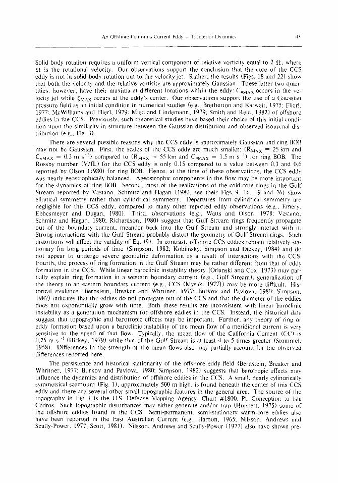
An Offshore California Current Eddy -- I: Interior Dynamics 43
Solid body rotation requires a uniform vertical component of relative vorticity equal to 2 [~, where ~ is the rotational velocity. Our observations support the conclusion that the core of the CCS eddy is not in solid-body rotation out to the velocity jet. Rather, the results (Figs. 18 and 22) show that both the velocity and the relative vorticity are approximately Gaussian. These latter two quan- tities, however, have their maxima at different locations within the eddy: COMAX Occurs in the ve- locity jet while ~JMAX occurs at the eddy's center. Our observations support the use of a Gaussian pressure field as an initial condition in numerical studies (e.g., Bretherton and Karweit, 1975: Flierl, 1977: McWilliams and Flierl, 1979; Mied and Lindemann, 1979: Smith and Reid, 1982) of offshore eddies in the CCS. Previously, such theoretical studies have based their choice of this initial condi- tion upon the similarity in structure between the Gaussian distribution and observed isopycnal dis- tribution (e.g., Fig. 3).
There are several possible reasons why the CCS eddy is approximately Gaussian and ring BOB may not be Gaussian. First, the scales of the CCS eddy are much smaller : (RMAx = 25 km and C;;MA X = 0.3 m s - t) compared to (RMAx ~ 55 km and COMAX = 1.5 m s 1) for ring BOB. Tile Rossby number (V/fL) for the CCS eddy is only 0.15 compared to a value between 0.3 and 0.6 reported by Olson (1980) for ring BOB. Hence, at the time of these observations, the CCS eddy was nearly geostrophically balanced. Ageostrophic components in the flow may be more important for the dynamics of ring BOB. Second, most of the realizations of the cold-core rings in the Gulf Stream reported by Vastano, Schmitz and Hagan (1980, see their Figs. 9, 16, 19 and 26) show elliptical symmetry rather than cylindrical symmetry. Departures from cylindrical symmetry are negligible for this CCS eddy, compared to many other reported eddy observations (e.g., Emery, Ebbesmeyer and Dugan, 1980). Third, observations (e.g., Watts and Olson, 1978; Vastano, Schmitz and Hagan, 1980: Richardson, 1980) suggest that Gulf Stream rings frequently propagate out of the boundary current, meander back into the Gulf Stream and strongly interact with it. Strong interactions with the Gulf Stream probably distort the geometry of Gulf Stream rings. Such distortions will affect the validity of Eq. (9). In contrast, offshore CCS eddies remain relatively sta- tionary for long periods of time (Simpson, 1982; Koblinsky, Simpson and Dickey, 1984) and do not appear to undergo severe geometric deformation as a result of interactions with the CCS. Fourth, the process of ring formation in the Gulf Stream may be rather different from that of eddy formation in the CCS. While linear baroclinic instability theory (Orlanski and Cox, 1973) may par- tially explain ring formation in a western boundary current (e.g., Gulf Stream), generalization of the theory to an eastern boundary current (e.g., CCS (Mysak, 1977)) may be more difficult. His- torical evidence (Bernstein, Breaker and Whritner, 1977: Burkov and Pavlova, 1980: Simpson, 1982) indicates that the eddies do not propagate out of the CCS and that the diameter of the eddies does not exponentially grow with time. Both these results are inconsistent with linear baroclinic instability as a generation mechanism for offshore eddies in the CCS. Instead, the historical data suggest that topographic and barotropic effects may be important. Further, any theory of ring or eddy formation based upon a baroclinic instability of the mean flow of a meridional current is very sensitive to the speed of that flow. Typically, the mean flow of the California Current (CC) is 0.25 m s -I (Hickey, 1979) while that of the Gulf Stream is at least 4 to 5 times greater (Stommel, 1958). Differences in the strength of the mean flows also may partially account for the observed differences reported here.
The persistence and historical stationarity of the offshore eddy field (Bernstein, Breaker and Whritner, 1977: Burkov and Pavlova, 1980: Simpson, 1982) suggests that barotropic effects may influence the dynamics and distribution of offshore eddies in the CCS. A small, nearly cylindrically symmetrical seamount (Fig. 1), approximately 500 m high, is found beneath the center of this CCS eddy and there are several other small topographic features in the general area. The source of the topography in Fig. 1 is the U.S. Defense Mapping Agency, Chart #1800, Pt. Conception to Isla Cedros. Such topographic disturbances may either generate and/or trap (Huppert, 1975) some of the offshore eddies found in the CCS. Semi-permanent, semi-stationary warm-core eddies also have been reported in the East Australian Current (e.g., Hamon, 1965: Nilsson, Andrews and Scully-Power, 1977: Scott, 1981). Nilsson, Andrews and Scully-Power (1977) also have shown pre-

44 J . J . SIMPSON, T. D. DICKEY and C. J. KOBLINSKY
ferred areas of warm-core eddy formation. Both Nilsson, Andrews and Scully-Power (1977) and Scott (1981) have suggested that the persistence and permanency of these features may be linked to the known bottom topography, Other studies (Owens and Hogg, 1980; Hogg and Schmitz, 1980) provide evidence that topography can constrain the mean flow to closely follow isobaths.
The distributions of PV and o- 0 show that, between 250 and 600 m, lateral exchange is severely inhibited. Prior to the observations, however, lateral exchange may have occurred above 250 m, especially in a zone around the 26.4 isopycnal and at the base of the surface layer. Lateral exchange also may have occurred below 1000 m.
A strong thermal front is located along the NE quadrant of the eddy, while a strong haline front is located in the SW quadrant. The interaction of these surface frontal structures with the eddy was studied with satellite observations by Koblinsky, Simpson and Dickey (1984). Their analysis shows that, over a period of several months, bands of warm, salty water from the southwestern salinity front (feature E in Fig. 1, Koblinsky, Simpson and Dickey, 1984) wrapped around cooler coastal water (feature D in Fig. 1, Koblinsky, Simpson and Dickey, 1984). The satellite data also show that part of the colder coastal water was entrained into the center of the sur- face expression of the eddy. Simpson (1984) hypothesized that the lateral interleaving and mixing processes which occurred in the vicinity of these surface fronts produced highly diffusive water types at the surface, some of which were gravitationally unstable. In situ chemical evidence (Simpson, 1984) is consistent with the satellite observations cited above and further suggests that some of these diffusive water types then began to sink along density surfaces and may have contri- buted to the production of the deep frontal structures (down to --100 m) which appear in Figs. 2, 4 and 5. A more detailed discussion of frontal processes and cold-core formation processes is given by Simpson (1984).
Other observational evidence for the lateral entrainment of coastal waters into the eddy struc- tures of the CCS is provided by the work of Traganza, Conrad and Breaker (1981). They used both remote sensing and underway surface mapping techniques to follow an upwelled plume off Point Sur. They suggested that the plume developed into a large (--100 km diameter) feature which moved seaward and was fed by coastal upwelling water and interacted with the CC (possibly an eddy, see Fig. 4, Traganza, Conrad and Breaker, 1981) to form a "cyclonic upwelling system." Historical data show that cyclonic eddies are more frequent inshore than offshore in the CCS (e.g., Wyllie, 1966; Burkov and Pavlova, 1980). The data of Traganza, Conrad and Breaker (1981) also show that bands of coastal upwelled water can occur as elongated plumes which extend more than 250 km across the CC and have sharp thermal and chemical fronts. The observations of the inshore interaction of upwelling plumes with a cyclonic eddy system (Traganza, Conrad and Breaker, 1981) are consistent with observations offshore (Simpson, 1984: Haury, 1984) of similar interactions between coastal waters and this anticyclonic eddy system. Finally, lateral entrainment of coastal waters into warm-core eddy systems in the East Australian current also has been reported (Scott, 1978; 1981). These later observations are discussed further by Simpson (1984) in conjunc- tion with the chemical and phytoplankton biomass structure of this CCS eddy system.
The observations presented here, like those of most other ring and eddy studies, were not synoptic. CTD observations made with sufficiently small horizontal scales to adequately resolve the structure of a mesoscale eddy require several days (here nine) to complete. Concurrent with the observations, the eddy rotated so that previously sampled water could have been resampled at a new location. Simultaneously, the eddy may be spinning up or spinning down. Hence, caution must be exercised in the interpretation of observed asymmetrical differences in properties and dynamical structure sampled along the different radii of the eddy. For example, the isotherms (Fig. 2) within the subsurface eddy are on average 30-40 m deeper along the EW transect than along the NS transect. This means, along with corresponding differences between the NS and EW distributions of velocity, vorticity, kinetic energy, available potential energy, and anomaly structure, that the subsurface eddy may have been in the process of spin-up during the observational period.
An intercomparison between the properties and dynamical quantities sampled along different

An Offshore California Current Eddy -- I: Interior Dynamics 45
radii through an eddy is complicated further by our ability to adequately resolve the geometric center of the eddy. The distribution of the micronutrient nitrite (see Fig. 7, Simpson, 1984) shows a plug-like structure along the EW transect. This feature is conspicuously absent in the NS tran- sect. Chemical and biological evidence (Simpson, 1984; Haury, 1984) suggests that the NS transect did not go through the center of the eddy whereas the EW transect did. This possibility is con- sistent with the way in which the shipboard survey was taken. The line of NS transect was chosen solely on the basis of satellite data while the EW transect was adjusted according to data collected along the NS transect. If the NS transect did not pass through the center of the eddy and the EW transect did, then the implied intensification (e.g., spin-up) discussed above may simply be an artifact of imperfect geometric sampling. Other asymmetries in structure may have a depth depen- dence. For example, the mean slope of the isotherms (Fig. 2) slope upward in the upper regions of the three-layer system and downward in the lower regions.
Finally, it should be noted that the observed structure of the three-layer system is consistent with the structure which would have been produced by the coalescence of two warm-core eddies, both of inshore origin, prior to the experiment. Such a mechanism of formation is consistent with other observations (e.g., Cresswell, 1982) and recent theoretical studies (e.g., Gill and Griffiths, 1981; Hughes, 1982). A detailed statistical analysis of eddy structure (Emery, Ebbesmeyer and Dugan, 1980), however, shows that very few observed multi-layer eddy systems have the structural simplicity and symmetry of this CCS eddy system. If the multi-layer systems reported by Emery, Ebbesmeyer and Dugan (1980) resulted from a coalescence process, then it is statistically unlikely that such a coalescence process would produce an eddy system similar to this CCS eddy system. Unfortunately, our observations are insufficient to either conclusively exclude or establish eddy- eddy coalescence as a generation mechanism for the CCS three-layer system.
11. CONCLUSIONS
From January 9 to 17, 1981, detailed observations were made of the horizontal and vertical structure beneath one of the quasi-permanent semi-stationary mesoscale offshore eddy signatures in the California Current System (CCS) discussed by Bernstein, Breaker and Whritner (1977), Burkov and Pavlova (1980), and by Simpson (1982). The vertical sections of temperature and of density show the presence of a three-layer system. A subsurface warm-core eddy, whose diameter is approximately 150 km at the 7°C isotherm, is the dominant feature. A warm surface layer, which extends to a depth of 75 m, lies over the eddy. Between the warm surface layer and the subsurface warm-core eddy, there is a cold-core region which extends to a depth of about 200 m.
Vertical sections of salinity and of dissolved oxygen are entirely different from sections of temperature and density. Diagrams of water mass characteristics confirm that the core of the eddy above 600 m consisted of inshore water from the California Undercurrent (CU). The high salinity, low dissolved oxygen and warm temperature of this core water mass uniquely identify its source as the CU (Reid, Roden, and Wyllie, 1958; Wooster and Jones, 1970). Below about 700 m, local waters from the Deep Poleward Flow (DPF) have been incorporated into the eddy. The observed distributions of properties (T, S, o-0, 02) are inconsistent with a single, local generation process for the three-layer system.
The typical Rossby number for the eddy system was R0 --~ 0.1. Thus, at the time the observa- tions were made, the system as a whole was in near geostrophic balance, but this balance cannot be used to explain the distribution of water properties within the eddy. Radial distributions of angular velocity (C0/r) and of normalized gradient velocity show that the eddy was not in solid body rota- tion out to the velocity jet. Our observations of gradient velocity support the use of a Gaussian radial height field as an initial condition in eddy models (e.g., McWilliams and Flierl, 1979). Possi- ble reasons why CCS eddies may differ dynamically from Gulf Stream rings are discussed.
The distribution of the vertical component of relative vorticity consisted of a zone of negative

46 J . J . SIMPSON, T. D. DICKI!Y and C. J. KOBIANSK'~
vorticity whose m a x i m u m occurred at the center of the eddy, indicating anticyclonic mot ion. Out- side the eddy, zones of positive relative vorticity were found. The radial d is t r ibut ions of relative vorticity, like the velocity d is t r ibut ions , suppor t the use of a Gauss ian radial pressure field as an ini- tial condi t ion in numerica l s tudies of offshore mesoscale eddies in the CCS. The dis t r ibut ions of potential vorticity and potential densi ty show that fluid exchange be tween the three- layer system and the exter ior fluid may have occurred at the base of the surface layer and along a mixing zone associated with the 26.4 isopycnal surface.
The frontal s t ruc ture associated with the eddy, chemical ev idence (Simpson, 1984), and bio- logical d is t r ibut ions (Haury, 1984) show that coastal water (e.g., California Cur ren t (CC) water) con t inued 1o be en t ra ined into the upper sect ions of the system. This e n t r a i n m e n t makes the CCS eddy a different p h e n o m e n o n f rom cold-core rings in the G u l f St ream but ra ther similar to some warm-core eddies found in the East Austral ian Current .
The heat , salt and dissolved oxygen anomal ies support the earlier conclusion that the core of the warm-core eddy above 600 m consis ted of inshore water, which or iginated in the CU. The mass anomaly s t ruc ture also suppor ts this conclus ion and fu r ther suggests that the cold-core region may have initially fo rmed separately f rom the subsurface warm-core eddy. Bernste in , Breaker and Whr i t ne r (1977) suggested that the CC is an uns table flow, which cont inuous ly develops meande r s with wavelengths of several h u n d r e d ki lometers . They suggested that these meanders intensify over Lt period of several m o n t h s , separate f rom the mean flow, and create isolated eddies. The presence of CU water in the core of this eddy raises the quest ion of how CU water was t ranspor ted from the cont inenta l slope. Normally, the CU is restricted to over the cont inenta l slope (flickey, 1979; Reid, Roden and Wyllie, 1958). Addit ional eddy generat ion m e c h a n i s m s to those discussed by ge rns te in , Breaker and W h r i m e r (1977), are required to explain the dis t r ibut ion, persistence, and core composi t ion of offshore mesoscale eddies in the CCS.
Acknowledgements -- Special thanks to Prof. J. L. Reid for his continued support of this work. This work was supported by the State of California through the Marine Life Research Group (MLRG) of the Scripps Institution of Oceanography. The Physical and Chemical Oceanographic Data Facility took the measurements. All the computations for this paper were done on the UCSD VAX. We thank the UCSD Computer Center for the special systems capabilities which were used. David Wiesenhahn assisted with the new, revised, and final data processing and analysis. David Siegel assisted with the preliminary data processing. Special thanks to Fred Crowe, Nancy Hulbirt, and Renb Wagemakers of the MLRG Illustrations Group for the preparation of the figures. Sharon McBride and Ruth Ebey supervised the typing and final preparation of the manuscript. The MLRG Business Office worked hard to see that everything arrived on time; spe- cial thanks to Lari, Sadie and Marion. Without the assistance and skill of the Captain and crew of R.V. New Horizon, the measurements could not have been made. Part of this work was supported by a grant (to JJS) from the California Space Institute. The comments of the reviewers were helpful in the preparation of the final manuscript. TDD received support from the University of Southern California Department of Geological Sciences and Institute of Marine and Coastal Studies.
REFERENCES
BAINBRIDGE, A.E. (1981) GEOSECS ATLANTIC EXPEDITION, Volume 1, HYDROGRAPHIC" DATA, 19172-1973. International Decade of Ocean Exploration, National Science Foundation, Washington, DC, 121 pp.
BARBER, R.T., and R.L. SMITH (1981) Coastal upwelling ecosystems. In: Analysis o! Marine Ecosystems, A.R. Longhurst, editor, Academic Press, 31-68.
BARKLEY, R.A. (1968) Oceanographic Atlas of the Pacoqc Ocean. University of Hawaii Press, 20 pp., 158 figs. BARRETT, J.R. (1971) Available potential energy of Gulf Stream rings. Deep-Sea Research, 18, 1221-1231. BERNAL, P.A., and J.A. MCGOWAN (1981) Advection and upwelling in the California Current. In: Coastal Upwel-
ling, F.A. Richards, editor, Coastal and Estuarine Sciences, Vol. 1, American Geophysical Union, Washington, DC, 381-399.
BERNSTEIN, R.L., L. BREAKER, and R. WHRITNER (1977) California Current eddy formation: ship, air and satellite results. &'ience, 195, 353-359.
BRETHERTON, F.P., and M. KARWEIT (1975) Mid-ocean mesoscale modeling. In: Numerical Models o/Ocean Cir- culation~ National Academy of Sciences, Washington, DC, 237-249.

An Offshore California Current Eddy -- 1: Interior Dynamics 47
BROWN, D.M. (1962) Results of current measurements with drogues, 1958-1961. Scripps Institution of Oceanogra- phy Data Report, SIO Reference 62-27, 64 pp.
BURKOV, V.A., and Yu. V. PAVLOVA (1980) Description of the eddy field of the California Current. Oceanology, 20, 272-278.
CARPENTER, J.H. (1965) The Chesapeake Bay Institute technique for the Winkler dissolved oxygen method. Lim- nology and Oceanography, 10, 141-143.
CHELTON, D.B., P.A. BERNAL and J.A. MCGOWAN (1982) Large-scale interannual physical and biological interaction in the California Current. Journal of Marine Research, 40, 1095-1125.
C[tENEY, R.E., and P.L. RICHARDSON (1976) Observed decay of a cyclonic Gulf Stream ring. Deep-Sea Research, 23, 143-155.
CRESSWELL, G.R. (1982) The coalescence of two East Australian Current warm-core eddies. Science, 215, 161-164. ELLIOTT, B.A. (1979) Anticyclonic rings and the energetics of the circulation of the Gulf of Mexico. Ph.D. disserta-
tion, Texas A&M University, 188 pp. EMERY, W.J. (1975) Dynamic height from temperature profiles. Journal ~/'Physical Oceanography, 5, 369-375. EMERY, W.J., C.C. EBBESMEYER, and J.P. DUGAN (1980) The fraction of vertical isotherm deflections associ-
ated with eddies: an estimate from multiship XBT surveys. Journal o[" Physical Oceanography, 10,885-899. EMERY, W.J., and A. O'BR1EN (1978) Inferring salinity from temperature or depth for dynamic height computations
in the North Pacific. Atmosphere-Ocean, 16,348-366. FLEMING, R.H. (1955) Review of the oceanography of the northern Pacific. International North Pac(/w Fisheries Com-
munication Bulletin, 2, 44 pp. FL1ERL, G.R. (1977) The application of linear quasigeostrophic dynamics to Gulf Stream rings. Journal ¢~/Phvsical
Oceanograpt~v, 7, 365-379. FOFONOFF, N.P. (1962) Physical properties of sea water. In: The Sea, Vol. 1, M.N. Hill, editor, lnterscience, New
York, NY, 3-30. GILL, A.E., and R.W. GRIFFITHS (1981) Why should two anticyclonic eddies merge'? Ocean Modelling, 41, 10. HAMON, B.V. (1965) The East Australian Current, 1960-64. Deep-Sea Research, 12, 899-921. HAURY, L.R. (1984) An offshore eddy in the California Current System. Part IV: Plankton distributions. Progress in
Oceanography, this volume. HESS, S.L. (1959) Introduction to Theoretical Meteorology. Holt Publishing Company, New York, 362 pp. HICKEY, B.M. (1979) The California Current System - hypotheses and facts. Progress in Oceanography, 8, 191-279. HOGG, N.G., and W.J. SCHMITZ, Jr. (1980) A dynamical interpretation of low-frequency motions near very rough
topography -- the Charlie Gibbs Fracture Zone. Journal ~?fMarine Research, 38,215-248. HOLTON, J.R. (1972) An Introduction to Dynamic Meteorology. Academic Press, New York and London, 319 pp. HOSKINS, B.J. (1975) The geostrophic momentum approximation and the semi-geostrophic equations. Journal Qf~he
Atmospheric Sciences, 32,233-242. HUGHES, R.L. (1982) The energetics of merging anticyclonic eddies. Ocean 7vIodelling, 42, 7. HUPPERT, H.E. (1975) Some remarks on the initiation of inertial Taylor columns. Journal o['Fluid Mechanics, 67,
397-412. HUYER, A. (1977) Seasonal variation in the temperature, salinity and density over the continental shelf off Oregon.
Limnology and Oceanography, 22,442-453. HUYER, A., B.M. HICKEY, J.D. SMITH, R.L. SMITH, and R.D. PILLSBURY (1975) Alongshore coherence at
low frequencies in currents observed over the continental shelf off Oregon and Washington. Journal ~f Geophysical Research, 80, 3495-3585.
JOYCE, T.M., S.L. PATTERSON, and R.C. MILLARD, Jr. (1981) Anatomy of a cyclonic ring in the Drake Passage. Deep-Sea Res., 28, 1265-1287.
KENYON, K.E. (1983) Sections along 35°N in the Pacific. Deep-32~a Research, 30,349-369. KNAUSS, J.A. (1962) Observations of internal waves of tidal period made with neutrally-buoyant floats. Jm¢rnal ~/
Marine Research, 20, 111-118. KOBLINSKY, C.J., J.J. SIMPSON, and T.D. DICKEY (1984) An offshore eddy in the California Current System,
Part I1: Surface manifestation. Progress in Oceanograpl¢v, this volume. LORENZ, E.N. (1955) Available potential energy and the maintenance of the general circulation. Tellus, 7, 157-167. LYNN, R.J., K.A. BLISS, and L.E. EBER (1982) Vertical and horizontal distributions of seasonal mean temperature,
salinity, sigma-t, stability, dynamic height, oxygen and oxygen saturation in the California Current, 1958-1978. ('aICOFI Atlas 30, University of California, San Diego, 513 pp.
MCWILLIAMS, J.C., and G.R. FLIERL (1979) On the evolution of isolated non-linear vortices, with application to Gull" Stream rings. Journal ¢~l'Physical Oceanography, 9, 1155-1182.
MIED, R.P., and G.J. LINDEMANN (1979) The propagation and evolution of cyclonic Gulf Stream rings. Journal o/ Pt¢~,sical Oceanography, 9, 1183-1206.
MILLERO, F,J., C.T. CHEN, A. BRADSHAW, and K. SCHLIECIIER (1980) A new high pressure equation of state for seawater. Deep-Sea Research, 27, 255-264.
MILLERO, F.J., and A. POISSON (1981) Summary of data treatment for the UNESCO one atmosphere equation of state for seawater. UNESCO Technical Reports.

48 J . J . S~MPSON, T. D. DICKEY a n d C. J. KOBLINSKY
MILNE-THOMSON, L.M. (1968) Theoretical Hydrodynamics. The MacMillan Press Ltd., London and Basingstoke, 743 pp.
MYSAK, L.A. (1977) On the stability of the California Undercurrent off Vancouver Island. Journal ~/' Physical Oceanography, 7, 904-917.
NELEPO, B.A., Yu.M. KUFTARKOV, and V.K. KOSNYREV (1978) Effects of mesoscale eddies on ocean surface temperature, lzvestiya Atmospheric and Oceanic Physics, 14, 545-550.
NEUMANN, G., and W.J. PIERSON, Jr. (1966) Principles of Physical Oceanography, Prentice-Hall, Inc., Englewood Cliffs, N J, 545 pp.
NEWTON, C.W. (1961) Estimates of vertical motions and meridional heat exchange in Gulf Stream eddies and a com- parison with atmospheric disturbances. Journal of Geophysical Research, 66, 852-869.
NILSSON, C.S., J.C. ANDREWS, and P. SCULLY-POWER (1977) Observations of eddy formation off east Aus- tralia. Journal of Physical Oceanography, 7, 659-669.
NILSSON, C.S., and G.R. CRESSWELL (1981) The formation and evolution of East Australian Current warm-core eddies. Progress m Oceanography, 9, 133-183.
OLSON, D.B. (1980) The physical oceanography of two rings observed by the Cyclonic Ring Experiment, Part II: Dynamics. Journal of Physical Oceanography, 10, 514-527.
ORLANSKI, I., and M.D. COX (1973) Baroclinic instability in ocean currents. Geophysical Fluid Dynamics. 4, 297- 332.
OWENS, W.B., and N.G. HOGG (1980) Oceanic observations of stratified Taylor columns near a bump. Deep-Sea Research, 27A, 1029-1045.
PEDLOSKY, J. (1971) Geophysical fluid dynamics. In: Mathematical Problems in the Geophysical Sciences (William H. Reid, editor), Lectures in Applied Mathematics, Vol. 13, American Mathematical Society, Providence, RI, 1-60.
PERKIN, R.G., and E.L. LEWIS (1980) The Practical Salinity Scale 1978: Fitting the data. IEEE Journal o/'Oceanic Engineering, OE-5, 9-16.
PICKARD, G.L. (1964) Descriptive Physical Oceanography. Pergamon Press, Oxford, England, 214 pp. PYTKOWICZ, R.M., and D.R. KESTER (1966) Oxygen and phosphate as indicators for the deep intermediale waters
in the northeast Pacific Ocean. Deep-Sea Research, 13, 373-379 REID, J.L., Jr. (1956) Observations of internal tides in October 1950. Transactions c~[the American Geophysical Union,
37, 278-286. REID, J.L., Jr. (1962) Measurements of the California Countercurrent at a depth of 250 meters. Journal of Marine
Research, 20, 134-137. REID, J.L., Jr. (1963) Measurements of the California Countercurrent off Baja California. Journal of Geophysical
Research, 68, 4819-4822. REID, J.L., Jr. (1965a) Physical oceanography of the region near Point Arguello. Technical Report, Institute of
Marine Resources, University of California, IMR ReJerence 65-19. REID, J.L., Jr. (1965b) Intermediate Waters of the Pacific Ocean. Johns Hopkins Oceanographic Studies, 2, The Johns
Hopkins Press, 85 pp. REID, J.L., and A.W. MANTYLA (1978) On the mid-depth circulation of the north Pacific Ocean Journal q/P/z~si-
cal Oceanography, 8, 946-951. REID, J.L., Jr., G.I. RODEN, and J.G. WYLLIE (1958) Studies of the California Current System Cali/ornia
Cooperative Oceanic Fisheries Investigations, Progress Report, 1 July 1956 to 1 January 1958, 27-56. REID, J.L., Jr., and R.A. SCHWARTZLOSE (1962) Direct measurements of the Davidson Current off Central Cali-
fornia. Journal of Geophysical Research, 67, 2491-2497. REID, R.O., B.A. ELLIOT, and D.B. OLSON (1981) Available potential energy: a clarification. Journal o/' Physical
Oceanography, 11, 15-29. RICHARDSON, P.L. (1980) Gulf Stream ring trajectories. Journal of Physical Oceanography, 10, 90-104. ROBINSON, M.K. (1976) Atlas of North Pacific Ocean monthly mean temperatures and salinities of the surface layer.
Naval Oceanographic Office Reference Publication 2, 173 pp. SCHWARTZLOSE, R.A. (1963) Nearshore currents of the western United States and Baja California as measured by
drift bottles. California Cooperative Oceanic Fisheries Investigations, Progress Report, 7-1-60 to 6-3-62, Marine Research Committee, California Department of Fish & Game, Sacramento, CA, 15-22.
SCOTT, B.D. (1978) Hydrological features of a warm-core eddy and their biological implications. CSIRO, Australian Division of Fisheries and Oceanography, Marine Laboratory, Cronulla, Sidney, Australia, Report No 100, 18 pp.
SCOTT, B.D. (1981) Hydrological structure and phytoplankton distribution in the region of a warm-core eddy in the Tasman Sea. Australian Journal of Marine and Freshwater Research, 32,479-492.
SIMPSON, J.J. (1982) Offshore mesoscale eddies in the California Current System: Historical evidence. EOS, 63, 1004.
SIMPSON, J.J. (1984) An offshore eddy in the California Current System, Part IIl: Chemical structure. Progress in Oceanography, this volume.
SMITH, D.C., IV, and R.O. RElD (1982) A numerical study of nonffictional decay of mesoscale eddies. Journal oj Physical Oceanography, 12,244-255.

An Offshore California Current Eddy -- I: Interior Dynamics 49
SMITH, R.L. (1968) Upwelling. Oceanography and Marine Biology Annual Review, 6, 11-46. STOMMEL, H,S. (1965) The Gulf Stream, a Physical and Dynamical Description, 2nd edition, University of California
Press, 202 pp. TRAGANZA, E.D., J.C. CONRAD, and L.C. BREAKER (1981) Satellite observations of a "cyclonic nutrient upwel-
ling" and "giant plume" in the California Current. In: Coastal Upwelling -- Coast and Estuarine Science, Volume 1, F. A. Richards, editor, American Geophysical Union, 228-241.
UNESCO (1979) Ninth report of the Joint Panel on Oceanographic Tables and Standards. UNESCO Technical Papers in Marine Science, 30, 32 pp.
VASTANO, A.C., J.E. SCHMITZ, and D.E. HAGAN (1980) The physical oceanography of two rings observed by the Cyclonic Ring Experiment, Part I: Physical structures. Journal of Physical Oceanography, 10,493-513.
WATTS, D.R., and D.B. OLSON (1978) Gulf Stream ring coalescences with the Gulf Stream off Cape Hatteras. Sci- ence, 202,971-972.
WEBSTER, D. (1965) Webster's Seventh New Collegiate Dictionary. G. and C. Marion Company, Springfield, MA, 1,221 pp.
WEISS, R.F. (1970) The solubility of nitrogen, oxygen and argon in water and seawater. Deep-Sea Research, 17, 721- 735.
WOOSTER, W.S., and J.H. JONES (1970) California Undercurrent off northern Baja California. Journal ~f Marine Research, 28, 235-250.
WYLLIE, J.G. (1966) Geostrophic flow of the California Current at the surface and at 200 m. CaliJornia Cooperative Oceanic Fisheries Investigations Atlas No. 4, xii pp., and 288 charts.