An Oligopoly Model for Analyzing and Evaluating

(Re)-Assignments of Spectrum Licenses

Running head: (Re)-Assignments of Spectrum Licenses

Simon Loertscher∗ Leslie M. Marx†

August 11, 2014

∗Department of Economics, Level 4, FBE Building, 111 Barry Street, University of Melbourne, Victoria 3010,Australia. Email: simonl@unimelb.edu.au.

†Corresponding author. The Fuqua School of Business, Duke University, 100 Fuqua Drive, Durham, NC 27708,USA. Phone: 1-919-660-7762. Email: marx@duke.edu.

1

Abstract:

The Communications Act requires the Federal Communications Commission to assess whether

proposed spectrum license transactions serve the public interest, convenience, and necessity. We

review the FCC’s implementation of this component of the Act. We provide a tractable eco-

nomic model of competition among wireless service providers in which spectrum licenses are a cost-

reducing input. This model allows us to evaluate the effects of (re-)assigning spectrum licenses on

economic outcomes and to define operational measures of “warehousing” licenses. Calibrating the

model, we find little evidence of warehousing and that the approved Verizon-T-Mobile-SpectrumCo

transaction increased social surplus.

Keywords: Communications Act, FCC, spectrum licenses, warehousing

2

1 Introduction

The Communications Act of 1934 requires that the Federal Communications Commission (FCC)

evaluate spectrum license transactions to assess whether they serve the public interest, convenience,

and necessity. As stated in the FCC’s review of the 2012 transaction involving Verizon, T-Mobile,

and SpectrumCo,1 “The Communications Act requires the Commission to examine closely the

impact of spectrum aggregation on competition, innovation, and the efficient use of spectrum in

order to ensure that any transfer of control serves the public interest, convenience, and necessity.”

(Verizon-T-Mobile-SpectrumCo MO&O, para. 47)

We review the FCC’s implementation of this component of the Act as reflected in recent transac-

tions. When analyzing spectrum license transactions, the FCC has examined the effects of spectrum

aggregation on competition generally and consumer prices more specifically.2 In addition, the FCC

has raised concerns that are related to foreclosure in its analysis, including discussion of the issue

of the “warehousing” of spectrum.3

To organize the discussion and analysis, we present a model of price competition among a small

number of firms, where the firms in the oligopoly offer differentiated products and face capacity

constraints. This model allows us to evaluate the effects of (re-)assigning spectrum licenses on

economic outcomes including consumer prices, consumer surplus, and social welfare. The model is

1Memorandum Opinion and Order and Declaratory Ruling in the Matter of Applications of

Cellco Partnership d/b/a Verizon Wireless and SpectrumCo LLC et al., WT Docket Nos. 12-

4, 12-175, Adopted August 21, 2012 (hereafter Verizon-T-Mobile-SpectrumCo MO&O), available at

http://hraunfoss.fcc.gov/edocs_public/attachmatch/FCC-12-95A1.pdf.

2See, e.g., Verizon-TMobile-SpectrumCo MO&O, para. 76.

3See, e.g., Verizon-TMobile-SpectrumCo MO&O, paras. 68—72.

3

tractable but still rich enough to produce substantially different policy prescriptions that depend

on the nature of demand and the allocation of spectrum licenses. For example, when all firms face

the same demand functions, the assignment of spectrum licenses that maximizes consumer surplus

typically involves all firms’ holding the same amount of spectrum; however, when some firms face

stronger demand than others, in order to maximize consumer surplus the firms that face stronger

demand must be assigned relatively more spectrum licenses so that they have larger capacities with

which to serve their customers. Moreover, we can use the model to offer formal definitions of the

otherwise typically vague notion of warehousing spectrum, which appears in policy debates.

We define two measures that are relevant for evaluating concerns of spectrum warehousing.

First, we define the foreclosure-share measure of warehousing incentives, which is based on firms’

relative foreclosure and use values for incremental capacity; this measure addresses the incentive for

warehousing and hence the likelihood that warehousing incentives might distort market outcomes.

Second, we define the excess-capacity measure of warehousing, which is based on how firms’ actual

capacities compare with capacities in a hypothetical environment in which there is no incentive

for warehousing.4 This measure of warehousing captures the possibility of distortions in current

spectrum holdings.

We apply the model to the spectrum license transaction in 2012 that involved Verizon, T-

Mobile, and SpectrumCo. To perform this analysis, we choose parameters for the model so that

the pretransaction revenue shares of the top four mobile wireless service providers match their

actual relative revenue shares. Given this calibration of the model, we find that the transaction

4More precisely, we consider a theoretical environment in which the market supply of capacity is perfectly price

elastic and perfectly competitive. This means that firms can purchase as much spectrum as they want at a fixed

market price for spectrum.

4

increased both consumer surplus and overall welfare.

Analyzing the issue of warehousing of spectrum within the context of our model, we find little

evidence of warehousing motives for the transaction. As we show, prior to the transaction, the

foreclosure-share measure of warehousing incentive was similar for Verizon and T-Mobile, which

suggests that foreclosure incentives were unlikely to affect the outcome. In addition, we show

that following the transaction, the excess-supply measure of warehousing showed little evidence

for concern. We find that actual capacities are no more than 10% greater than theoretical no-

warehousing capacities for Verizon and AT&T, which are the wireless providers for whom concerns

related to warehousing have most often been raised.

The methodology presented here is potentially useful for the analysis of the economic effects of

future license transfers. In addition, if one has a good estimate of how demand will change after a

merger, the model could also be applied to the analysis of horizontal mergers. Lastly, the model

is quantitatively plausible insofar as when it is calibrated to match the market shares prior to the

reassignment of spectrum licenses between Verizon, T-Mobile, and SpectrumCo in 2012, the price

for capacity implied by the model is close to the average prices for AWS-1 spectrum licences in

FCC Auction 66.5

In this paper, we first elaborate more on the foundation in the Communications Act for the

FCC’s review of spectrum license transactions in Section 2. Section 3 presents the economic model

that we use for analyzing such transactions. In Section 4 we apply the model to the Verizon-T-

5 In the model, the price for capacity is taken as given by the firms. To derive an implied price for capacity,

we calculate the price that minimizes the sum of squared deviations between equilibrium capacities and empirically

observed capacities. The dollar prices per MHz*Pop are, respectively, $0.45 and $0.53 for the model and for Auction

66.

5

Mobile-SpectrumCo transaction. Section 5 concludes with a discussion.

2 The Communications Act and the FCC

The Communications Act of 1934,6 as revised, specifically Section 310 of the Act, requires firms to

seek approval from the FCC to transfer control of spectrum licenses:

No construction permit or station license, or any rights thereunder, shall be trans-

ferred, assigned, or disposed of in any manner, voluntarily or involuntarily, directly or

indirectly, or by transfer of control of any corporation holding such permit or license,

to any person except upon application to the Commission and upon finding by the

Commission that the public interest, convenience, and necessity will be served thereby.

Any such application shall be disposed of as if the proposed transferee or assignee were

making application under section 308 for the permit or license in question; but in act-

ing thereon the Commission may not consider whether the public interest, convenience,

and necessity might be served by the transfer, assignment, or disposal of the permit or

license to a person other than the proposed transferee or assignee. (Communications

Act of 1934, Section 310(d), emphasis added)

As indicated in the highlighted text above, the Communications Act sets out the standard for

approval of a transaction that the FCC must find that the transaction serves the public interest,

convenience, and necessity.

The FCC analyzes the benefits versus disadvantages presented by each case, grounded in this

section of Act. For example, as stated in the FCC order in the Verizon-T-Mobile-SpectrumCo

6Available at http://transition.fcc.gov/Reports/1934new.pdf.

6

transaction of 2012:

Pursuant to Section 310(d) of the Communications Act, we must determine whether ap-

plicants have demonstrated that a proposed assignment of licenses will serve the public

interest, convenience, and necessity. In making this assessment, we first assess whether

the proposed transaction complies with the specific provisions of the Communications

Act, other applicable statutes, and the Commission’s rules. If the transaction does

not violate a statute or rule, we next consider whether the transaction could result in

public interest harms by substantially frustrating or impairing the objectives or imple-

mentation of the Communications Act or related statutes. We then employ a balancing

test weighing any potential public interest harms of the proposed transaction against

any potential public interest benefits. The applicants bear the burden of proving, by

a preponderance of the evidence, that the proposed transaction, on balance, will serve

the public interest. (Verizon-T-Mobile-SpectrumCo MO&O, para. 28)

The FCC elaborates on the aims of the Communications Act in its order in the AT&T-

Qualcomm transaction of 2001,7 stating:

Our public interest evaluation also necessarily encompasses the “broad aims of the Com-

munications Act,” which include, among other things, a deeply rooted preference for

preserving and enhancing competition in relevant markets, accelerating private sector

deployment of advanced services, promoting a diversity of license holdings, and generally

managing the spectrum in the public interest. Our public interest analysis also often

7Order in the Matter of Application of AT&T Inc. and Qualcomm Incorporated, WT Docket No. 11-18, Adopted

December 22, 2011 (hereafter AT&T-Qualcomm Order).

7

entails assessing whether the proposed transaction will affect the quality of communica-

tions services or will result in the provision of new or additional services to consumers.

In conducting this analysis, we may consider technological and market changes, and the

nature, complexity, and speed of change of, as well as trends within, the communications

industry. (AT&T-Qualcomm Order, para. 24)

In the AT&T-Qualcomm Order, the FCC clarifies the role of separate reviews by the FCC and

Department of Justice, stating:

Our competitive analysis, which forms an important part of the public interest evalua-

tion, is informed by, but not limited to, traditional antitrust principles. The Department

of Justice’s (DOJ) review is limited solely to an examination of the competitive effects

of the acquisition, without reference to various public interest considerations. In ad-

dition, DOJ’s competitive review of communications mergers is pursuant to section 7

of the Clayton Act: if it wishes to block a merger, it must demonstrate to a court

that the merger may substantially lessen competition or tend to create a monopoly. By

contrast, the Commission’s review of the competitive effects of a transaction under the

public interest standard is broader: for example, it considers whether a transaction will

enhance, rather than merely preserve, existing competition, and takes a more extensive

view of potential and future competition and the impact on the relevant market, includ-

ing longer-term impacts. If we are unable to find that the proposed transaction serves

the public interest for any reason, or if the record presents a substantial and material

question of fact, we must designate the Application for hearing. (AT&T-Qualcomm

Order, para. 25)

8

The Communications Act gives the FCC authority to impose conditions on transactions as long

as those conditions are consistent with the applicable law. This authority is grounded in Section

303(r) of the Communications Act, which states that “Except as otherwise provided in this Act,

the Commission from time to time, as public convenience, interest, or necessity requires” shall:

Make such rules and regulations and prescribe such restrictions and conditions, not

inconsistent with law, as may be necessary to carry out the provisions of this Act, or

any international radio or wire communications treaty or convention, or regulations

annexed thereto, including any treaty or convention insofar as it relates to the use of

radio, to which the United States is or may hereafter become a party. (Communications

Act of 1934, Section 303(r))

The FCC summarizes the authority that has been granted to it in this section of the Act as it

applies to a spectrum license transfer as follows:

Our analysis recognizes that a proposed transaction may lead to both beneficial and

harmful consequences. Section 303(r) of the Communications Act authorizes the Com-

mission to prescribe restrictions or conditions not inconsistent with law that may be

necessary to carry out the provisions of the Communications Act. In using this broad

authority, the Commission has generally imposed conditions to remedy specific harms

likely to arise from the transaction or to help ensure the realization of potential benefits

promised for the transaction. (AT&T-Qualcomm Order, para. 26)

9

3 Model

In this section, we develop an oligopoly model that is representative of the market for mobile wireless

services in that it captures price competition among firms whose products differ in their desirability

to consumers and in which firms have varying capacities. In Section 4, we relate these capacity

levels to firms’ spectrum holdings. This model allows us to capture interactions in a market where

firms produce heterogeneous products and consumers make their purchase decisions based on the

firms’ prices and quality levels.

3.1 Setup

The demand side of our model is based on the model of Singh and Vives (1984). In particular,

we employ Häckner’s (2000) extension of Singh and Vives (1984) to the case of more than two

firms. There are goods or services, indexed = 1 , each of which is produced by a profit-

maximizing single-product firm with the same index, and a representative, price-taking consumer

that maximizes its utility from services q = (1 ) purchased minus its expenditure p · q,

where p = (1 ) is the vector of prices and where “·” denotes the inner product. That is, the

consumer solves the problem maxq(q)− p · q, where for analytical convenience (q) is assumed

to be of the form

(q) ≡X=1

− 12

2 −

X

(1)

This model can be viewed as assigning each firm a baseline consumer value for firm ’s product

of . The parameter is the marginal utility to the representative consumer of firm ’s product

when q = 0.8 We can view as reflecting the match of firm ’s product with the consumer’s

8 In our model formulation, capacity enters through the firms’ cost functions; however, one might consider an

10

preferences or the quality of firm ’s product. In what follows, we refer to as a quality parameter.

The model also fixes the degree of substitutability ∈ [0 1] between the services of firms

and (for 6= ).

Each firm faces demand for its services that depends on its quality and its price and the

qualities a− and prices p− of its rivals. For simplicity, in the main body of the paper, we assume

that for all = 1 and that for all 6= = . As a robustness check, we explore alternatives in

Section 4.3.2. The assumptions on the substitutability parameter imply that the substitution effects

among the firms are symmetric, while the combined assumptions force any empirically observed

differences in market shares to be explained by the vector of qualities a.9 As is well known, the

utility function in (1) gives rise to a linear demand structure with inverse demands given by, for

∈ {1 } = − − P

6= . It will sometimes be useful to write the quantity demanded

from firm given prices as (p−).

On the supply side, we consider an oligopoly game in which firms choose prices. Payoffs are

equal to profits, which for firm are = − ( ), where ( ) = () is the cost

of producing quantity given capacity with () satisfying 0 and 00 0. Observe that this

implies that for fixed the marginal cost of production is increasing in while ( ) =

( ) for 0. That is, the long-run cost function reflects a production technology that

exhibits constant returns to scale. For analytical ease, we assume () = 2, so that firm has cost

alternative formulation in which a firm’s capacity enters the demand function for its product by altering the marginal

utility to the consumer of that firm’s product.

9 In Section 4.3, we explore two alternative calibrations. First, we assume that firms differ with respect to the slope

parameters rather than the intercept . Second, we assume that some revenue accrues to firm from consumers

whose prices and consumption levels are predetermined (while again imposing heterogeneity with respect to the ’s

and setting = 1 for all ).

11

( ) =2. Thus, the marginal cost of firm is

()

= 2. We use (subgame perfect)

Nash equilibrium as our solution concept.

In this model, consumer surplus is

(qp) ≡ (q)− p · q

If we let k = (1 ) be the vector of capacity inputs, welfare, (qk), is consumer surplus

plus the sum of firms’ profits, which is equal to

(qk) ≡ (q)−X=1

( )

Capacities k, qualities a and the substitution parameter are given and common knowledge before

firms simultaneously set prices.

Accordingly, equilibrium prices p∗(k) = (∗1(k) ∗(k)) satisfy for all ∈ {1 }

∗ (k) ∈ argmax

(p∗−)− ((p

∗−) ). (2)

For notational simplicity, we sometimes use ∗ to denote (p∗), and we sometimes also write

∗ (k) to emphasize the dependence of equilibrium quantities on the firms’ capacities.

3.2 Analytic results

In order to explore the implications of this model for the effects described above, consider the

restriction to = 2. We assume that parameters are such that equilibrium quantities are positive

for both firms. The necessary and sufficient condition for this is:

2 + 2− 2

2 + 2− 2

(3)

where the first inequality relates to 0 and the second to 0. To see this, note that

∗ =((2 + (2− 2))− )

4 + 2(2− 2)2 + (4 + 4(1 + )− 2(2 + 5))

12

The denominator is positive,10 and the numerator is positive when (2 + (2− 2))− 0

which can be rewritten as 2+2−2

as in (3).

Key concerns in spectrum license transactions include the effect of the transaction on prices,

output, and consumer surplus. Viewing spectrum holdings as capacity in the model, we can analyze

the effects of transactions that transfer spectrum licenses among firms. In Section 3.2.1, we consider

the effects on prices and quantities of marginal changes in capacity. In Section 3.2.2, we consider

the effects of discrete shifts in capacity from one firm to the other. In Section 3.2.3, we show that

when firms are symmetric and total capacity is sufficiently large, consumer surplus is maximized in

the model when capacity is assigned so as to minimize the concentration in the industry. In Section

4, we consider asymmetric firms and show that in that case this result no longer holds–consumer

surplus may be increased by assigning relatively more capacity to higher quality firms. Finally, in

Section 3.2.4, we discuss the notions of warehousing and the “use” versus “foreclosure” value of

spectrum within the context of the model.

3.2.1 Marginal changes in capacity

As shown below, a marginal increase in the capacity of firm which lowers firm ’s marginal cost,

results in an equilibrium in which both firms have lower prices. Firm ’s quantity increases, but

firm ’s quantity decreases. Although firm lowers its price, that is not sufficient to outweigh the

effect of the decrease in its rival’s price on its quantity. However, total quantity increases.

10To see that the denominator is positive, note that it is minimized at = 1 and is positive when evaluated at

= 1.

13

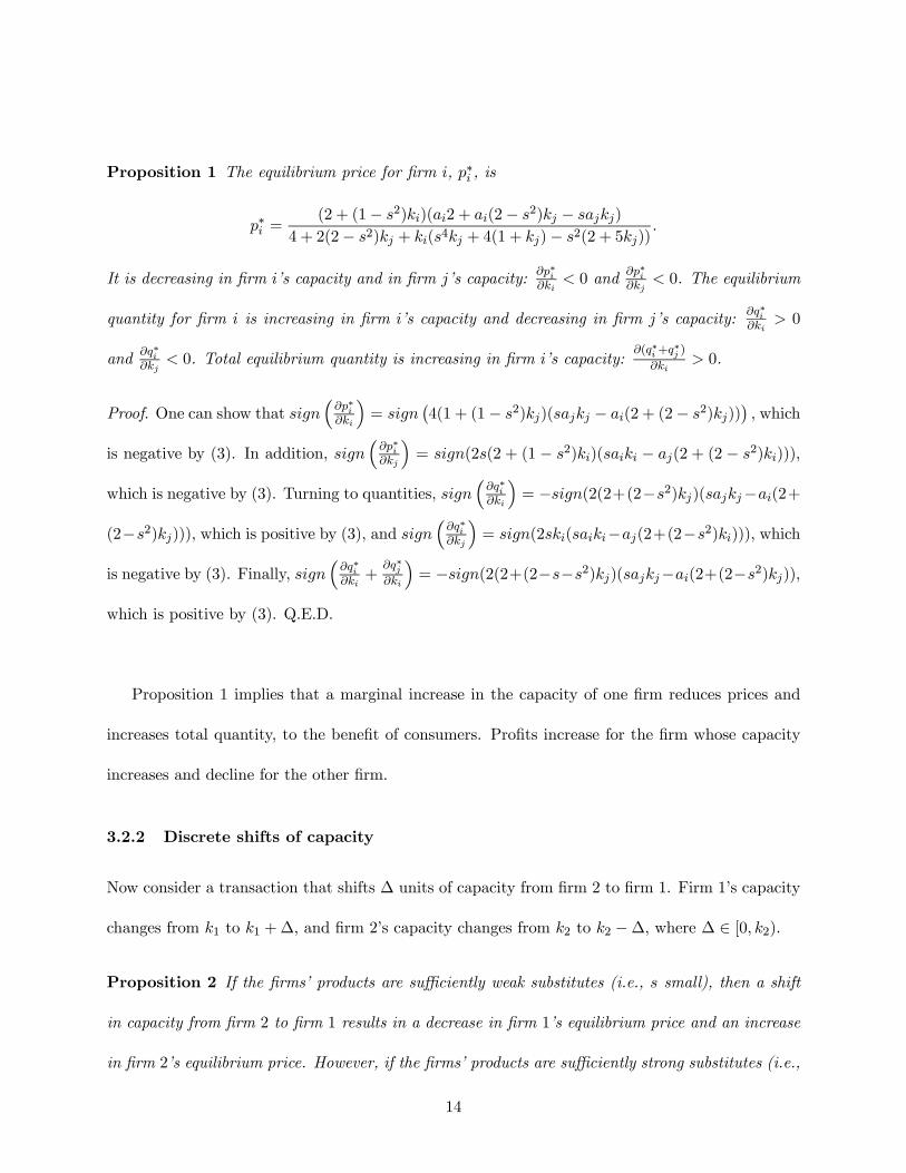
Proposition 1 The equilibrium price for firm , ∗ , is

∗ =(2 + (1− 2))(2 + (2− 2) − )

4 + 2(2− 2) + (4 + 4(1 + )− 2(2 + 5))

It is decreasing in firm ’s capacity and in firm ’s capacity:∗

0 and∗

0. The equilibrium

quantity for firm is increasing in firm ’s capacity and decreasing in firm ’s capacity:∗

0

and∗

0. Total equilibrium quantity is increasing in firm ’s capacity:(∗+

∗ )

0.

Proof. One can show that ³∗

´=

¡4(1 + (1− 2))( − (2 + (2− 2)))

¢ which

is negative by (3). In addition, ³∗

´= (2(2 + (1 − 2))( − (2 + (2 − 2))))

which is negative by (3). Turning to quantities, ³∗

´= −(2(2+(2−2))(−(2+

(2−2)))) which is positive by (3), and ³∗

´= (2(−(2+(2−2)))) which

is negative by (3). Finally, ³∗

+∗

´= −(2(2+(2−−2))(−(2+(2−2)))

which is positive by (3). Q.E.D.

Proposition 1 implies that a marginal increase in the capacity of one firm reduces prices and

increases total quantity, to the benefit of consumers. Profits increase for the firm whose capacity

increases and decline for the other firm.

3.2.2 Discrete shifts of capacity

Now consider a transaction that shifts ∆ units of capacity from firm 2 to firm 1. Firm 1’s capacity

changes from 1 to 1 +∆ and firm 2’s capacity changes from 2 to 2 −∆, where ∆ ∈ [0 2).

Proposition 2 If the firms’ products are sufficiently weak substitutes (i.e., small), then a shift

in capacity from firm 2 to firm 1 results in a decrease in firm 1’s equilibrium price and an increase

in firm 2’s equilibrium price. However, if the firms’ products are sufficiently strong substitutes (i.e.,

14

large), then the effect of the shift depends on which firm has higher quality (as measured by 1

and 2): if firm 1 has higher (resp. lower) quality, the shift results in a decrease (resp. increase) in

firm 1’s equilibrium price and an increase (resp. decrease) in firm 2’s equilibrium price.

Proof. One can show that ∗1(1 +∆ 2 −∆)− ∗1(1 2) is negative for 1 2 and sufficiently

large or for sufficiently small, but it is positive for 1 2 and sufficiently large. In addition,

one can show that ∗2(1 +∆ 2 −∆)− ∗2(1 2) is positive for 2 1 and sufficiently large or

for sufficiently small, but it is negative for 1 2 and sufficiently large. Q.E.D.

Viewing as a measure of firm ’s quality, a transfer of capacity to the lower quality firm causes

that firm to increase its prices when products are sufficiently close substitutes. (The dominant effect

is the restriction in capacity to the higher quality firm, causing that firm to increase its prices and,

given that in this model prices are strategic complements, for the lower quality firm to increase

its price as well.) Shifting capacity to the higher quality firm causes prices to decrease. Shifting

capacity to a firm with few good substitutes causes it to lower its price.

The transfer of capacity away from a firm causes its price to go up, unless it is the low quality

firm and products are highly substitutable, in which case the dominant effect can be the decrease

in rival’s price, which leads the firm to decrease its price.

As one would expect, shifting capacity can result in a lower price for the firm gaining capacity

and a lower price for the firm losing capacity, but it is possible to have other effects. In particular,

when products are highly substitutable, shifts in capacity to the higher quality firm can cause both

prices to go down, and shifts in capacity to the lower quality firm can cause both prices to go up.

In the next proposition, we consider the effects on quantity.

15

Proposition 3 If the firms’ products are sufficiently weak substitutes ( small), or if the firms are

sufficiently symmetric (1 ≈ 2) and the products are sufficiently strong substitutes ( small), then

a shift in capacity from firm 2 to firm 1 increases firm 1’s equilibrium quantity and decreases firm

2’s equilibrium quantity.

Proof. Letting = 0 one can show that ∗1(1+∆ 2−∆)− ∗1(1 2) is equal to∆1

2(1+1)(1+∆+1)

which is positive. In addition, at = 1 (∗1(1+∆ 2−∆)− ∗1(1 2)) = (∆(21+(1−

2 +∆) (2 − 1))) which is positive for |1 − 2| sufficiently small. Letting = 0 ∗2(1 +∆ 2 −

∆) − ∗2(1 2) is equal to−∆2

2(1+(2−∆))(1+2) which is negative. Finally, at = 1 (∗2(1 +

∆ 2 −∆)− ∗2(1 2)) = (∆(−22 + (1 − 2 +∆)(1 − 2))), which is negative for |1 − 2|

sufficiently small. Q.E.D.

Proposition 3 shows that, as one would expect, shifting capacity between firms tends to increase

the output of the firm receiving the capacity and decrease the output of the firm giving up the

capacity.

We can also consider the effect of a shift in capacity on the equilibrium output per unit of

capacity: i.e., the intensity with which capacity is utilized.

Proposition 4 If the firms’ products are sufficiently weak substitutes ( small), then a shift in

capacity from firm 2 to firm 1 results in a decrease in firm 1’s equilibrium output per unit of

capacity and an increase in firm 2’s equilibrium output per unit of capacity. However, if the firms’

products are sufficiently strong substitutes ( large), then the effect of the shift depends on which

firm has higher quality (as measured by 1 and 2): if firm 1 has higher (resp. lower) quality, the

shift results in a decrease (resp. increase) in firm 1’s equilibrium output per unit of capacity and an

16

increase (resp. decrease) in firm 2’s equilibrium output per unit of capacity.

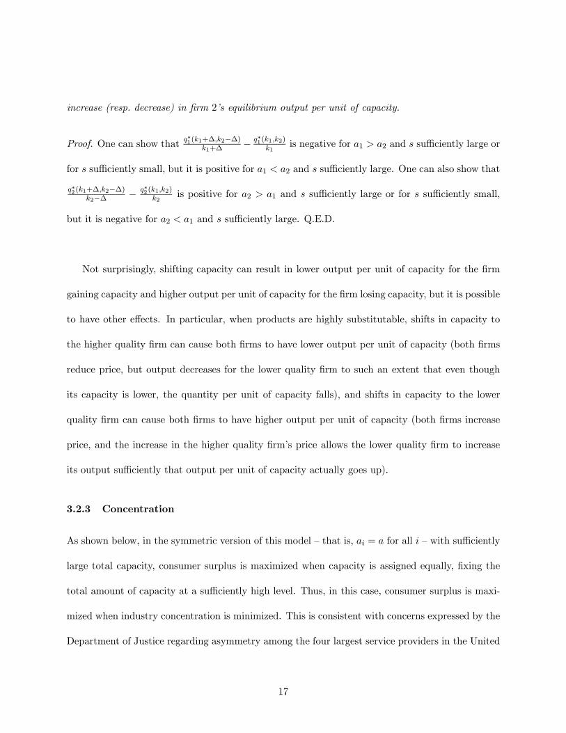
Proof. One can show that∗1(1+∆2−∆)

1+∆− ∗1(12)

1is negative for 1 2 and sufficiently large or

for sufficiently small, but it is positive for 1 2 and sufficiently large. One can also show that

∗2(1+∆2−∆)2−∆ − ∗2(12)

2is positive for 2 1 and sufficiently large or for sufficiently small,

but it is negative for 2 1 and sufficiently large. Q.E.D.

Not surprisingly, shifting capacity can result in lower output per unit of capacity for the firm

gaining capacity and higher output per unit of capacity for the firm losing capacity, but it is possible

to have other effects. In particular, when products are highly substitutable, shifts in capacity to

the higher quality firm can cause both firms to have lower output per unit of capacity (both firms

reduce price, but output decreases for the lower quality firm to such an extent that even though

its capacity is lower, the quantity per unit of capacity falls), and shifts in capacity to the lower

quality firm can cause both firms to have higher output per unit of capacity (both firms increase

price, and the increase in the higher quality firm’s price allows the lower quality firm to increase

its output sufficiently that output per unit of capacity actually goes up).

3.2.3 Concentration

As shown below, in the symmetric version of this model — that is, = for all — with sufficiently

large total capacity, consumer surplus is maximized when capacity is assigned equally, fixing the

total amount of capacity at a sufficiently high level. Thus, in this case, consumer surplus is maxi-

mized when industry concentration is minimized. This is consistent with concerns expressed by the

Department of Justice regarding asymmetry among the four largest service providers in the United

17

States;11 however, as we show, when firms vary in quality levels, shifts in capacity that increase

concentration can increase consumer surplus.

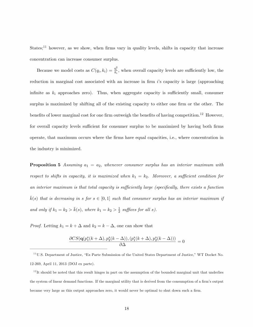
Because we model costs as ( ) =2 when overall capacity levels are sufficiently low, the

reduction in marginal cost associated with an increase in firm ’s capacity is large (approaching

infinite as approaches zero). Thus, when aggregate capacity is sufficiently small, consumer

surplus is maximized by shifting all of the existing capacity to either one firm or the other. The

benefits of lower marginal cost for one firm outweigh the benefits of having competition.12 However,

for overall capacity levels sufficient for consumer surplus to be maximized by having both firms

operate, that maximum occurs where the firms have equal capacities, i.e., where concentration in

the industry is minimized.

Proposition 5 Assuming 1 = 2 whenever consumer surplus has an interior maximum with

respect to shifts in capacity, it is maximized when 1 = 2. Moreover, a sufficient condition for

an interior maximum is that total capacity is sufficiently large (specifically, there exists a function

() that is decreasing in for ∈ [0 1] such that consumer surplus has an interior maximum if

and only if 1 = 2 () where 1 = 2 12suffices for all ).

Proof. Letting 1 = +∆ and 2 = −∆ one can show that

(q(∗1( +∆) ∗2( −∆)) (∗1( +∆) ∗2( −∆)))

∆= 0

11U.S. Department of Justice, “Ex Parte Submission of the United States Department of Justice,” WT Docket No.

12-269, April 11, 2013 (DOJ ex parte).

12 It should be noted that this result hinges in part on the assumption of the bounded marginal unit that underlies

the system of linear demand functions. If the marginal utility that is derived from the consumption of a firm’s output

became very large as this output approaches zero, it would never be optimal to shut down such a firm.

18

if and only if ∆ = 0, where consumer surplus is strictly concave in ∆ at ∆ = 0 if and only if

() ≡ 4³2 + 5+ 32 +

√36 + 52+ 132 − 23 + 4

´, where 0() 0 for ∈ [0 1] and

(0) = 12. Thus, for () consumer surplus is quasiconcave in ∆, with a unique maximum at

∆ = 0. Q.E.D.

In contrast to the result of Proposition 5, as we show below, if the firms are asymmetric with

respect to their quality parameters, then consumer surplus is not maximized by endowing each

firm with the same level of capacity. In that case, maximizing consumer surplus requires assigning

relative more of the capacity to the higher quality firm. In this sense, the model is rich enough to

generate substantially different optimal policy prescriptions as a function of the parameter values.

3.2.4 Warehousing

Concerns have been raised regarding the possibility that wireless service providers might purchase

spectrum not for the purpose of putting it to use to serve customers, but rather to prevent rivals

from having access to the spectrum, which is sometimes referred to as warehousing.13 One measure

taken by the FCC that can be viewed as a response to concerns about warehousing is that the FCC

imposes build-out requirements on holders of spectrum licenses. These build-out requirements are

aimed at minimizing the potential for firms to employ warehousing strategies.

We next discuss a number of different ways in which one might try to formalize the notion of

warehousing within the context of our model.

For models with constant returns to scale technologies in which the input is fixed in the short

run (which give rise to cost functions of the form ( ) = () with 0 0 and 00 0),

13See, e.g., DOJ ex parte, 2013.

19

it is well known that a unilateral increase in firm ’s capacity induces firm to use its capacity

less intensively in the sense that ∗ (k) decreases in (see e.g. Riordan, 1998, and Loertscher

and Reisinger, 2014a). The intuition is simply that increases in capacity decrease the marginal

cost of production for a given quantity, which induces the firm to produce more. But given that it

produces a larger quantity, the firm incurs a larger loss on the inframarginal units. Therefore, at

an optimum, its marginal gain must also be larger, which can only occur if ∗ (k) decreases. All

else equal, therefore, increases in capacity induce a firm to use capacity less intensively within the

present model.

Though this inverse relationship seems to be a sensible feature of the model, there is little sense

in defining “warehousing” in this way because it would be automatically implied by any unilateral

increase in capacity and optimizing behavior. Despite the above mechanics, our model is consistent

with the empirical observation that larger firms use capacities more intensively, that is with larger

firms having larger ratios ∗ (k) (irrespective of whether size is measured in terms of capacity or

market shares) because firm may be large because its quality as captured by the parameter is

high.

Differences in the quality parameters are consistent with the U.S. wireless market as portrayed

by Shapiro, et al. (2013). In Table 1, we summarize evidence that is provided by Shapiro, et al.

(2013, Table 4), which shows that the largest wireless carriers in the United States use their

spectrum more intensively than do certain smaller wireless carriers.

20

Table 1: Intensity of use of spectrum by wireless carriers

CarrierSubscribers

(millions)

Spectrum

(MHz)

Million subscribers

per MHz spectrum

Verizon Wireless 111 107 1.04

AT&T Mobility 106 88 1.20

Sprint Nextel 56 53 1.06

T-Mobile USA 33 57 0.58

MetroPCS 9 9 1.00

U.S. Cellular 6 9 0.67

Leap Wireless 6 9 0.67

Source: Shapiro, et al. (2013, Table 4)

Our first formalization of warehousing addresses the hypothetical question of how much a firm

would be willing to pay for an additional block of capacity in order to prevent a rival from receiving

it, relative to its own use value for the input. This question relates to the incentive for warehousing.

We define the foreclosure-share measure of warehousing incentive based on the distinction between

a firm’s “use” value and “foreclosure” value for spectrum as follows.

Suppose that an additional indivisible block of capacity ∆ 0 is offered for sale. Without

specifying the details of the selling mechanism, assume that if firm does not get ∆, then its rival

acquires it. We can then break down the value to firm from purchasing additional spectrum ∆

versus allowing rival to purchase it as follows:

( +∆ )− ( +∆) = (( +∆ )− ( ))

+ (( )− ( +∆))

21

where the first term on the right side of the equation is firm ’s “use” value for the spectrum and

the second term is its “foreclosure” value for the spectrum (see e.g. Ordover, et al., 1990).

If foreclosure values are sufficiently large relative to use values that they distort the ranking of

firms’ total values, then foreclosure concerns have the potential to affect market allocations relative

to what they would be if firms valued spectrum based only on their use values. Thus, we use a

firm’s foreclosure value as a share of its total value from purchasing additional spectrum ∆ to define

a foreclosure-share measure of warehousing incentive as follows:

foreclosure value

total value=

( )− ( +∆)

( +∆ )− ( +∆)

Larger values of the foreclosure-share measure of warehousing incentive, particularly when consid-

ered relative to other firms, give rise to greater concerns that warehousing incentives may distort

market outcomes.

The foreclosure-share measure of warehousing incentive, which focuses on the willingness to pay

for otherwise low-value capacity, presumes strong rivalry in the acquisition process by assuming

that if firm does not acquire the capacity, then some rival will. This corresponds to assuming

a perfectly inelastic supply of the additional unit of capacity. Conversely, one could assume a

perfectly elastic and competitive supply of capacity, so that at input price every firm can acquire

as much capacity as it desires.14 This gives rise to the excess-capacity measure of warehousing.

More specifically, to define the excess-capacity measure of warehousing, we fix the parameters of

14Riordan (1998) and Loertscher and Reisinger (2014a) analyze the intermediate case by assuming an upward

sloping, price elastic supply of capacity. Further work that makes the notion of warehousing operational in a model

in which oligopolistic firms exert market power on both input and output markets would seem valuable. For example,

one could suppose that the inverse market supply of capacity is () = 0 + 1 and calibrate based on (0 1)

as opposed to just 1 as in the exercise we describe.

22

demand, for example based on a calibration to market shares given firms’ capacities, and suppose

that capacity is competitively supplied at price . Then firm ’s problem is to choose capacity

to solve

max

∗ (k)∗ (k)− (∗ (k) )− .

This offers a way of endogenizing capacities. For a given , the implied equilibrium capacities

k∗() = (∗1() ∗()) can then be compared to their counterparts k = (1 ), where k may

be the empirical capacity levels or some alternative benchmark levels. Excess capacity relative to

implied equilibrium capacity,−∗ ()∗ ()

is our excess-capacity measure of warehousing. As mentioned

above, it provides a measure of warehousing based on a model of perfectly competitive and perfectly

elastic input supply.

In practice, however, it need not always be clear what the correct choice of is. One way

around this problem is to choose the that minimizesP

=1(− ∗ ())2. Letting be the solution

to this problem, one can then compare the capacities k with those associated with the hypothetical

competitive supply, taking−∗ ()∗ ()

as the excess-capacity measure of warehousing. Large values of

the excess-capacity measure of warehousing, particularly when considered relative to other firms,

would indicate that capacities are greater than those associated with the hypothetical competitive

supply and would be indicative of warehousing.15

15A natural conjecture is that the value of that is used to derive the theoretical equilibrium capacities affects

the size (and eventually the sign) of the various − ∗ ()’s but will not affect the ranking of the firms according to

− ∗ (). This conjecture is consistent with the exercises we perform below, where we show that the ranking is the

same when equilibrium values are computed using or the empirically observed price of capacity (see Tables 8 and

9 below for details).

23

3.3 Related literature

Dating back to Edgeworth (1925), the analysis of price competition with capacity constraints has a

long tradition in Industrial Organization, with important subsequent contributions by Levitan and

Shubik (1972), Kreps and Scheinkman (1983), Davidson and Deneckere (1986), and Deneckere and

Kovenock (1992, 1996); see Loertscher (2008) and the references therein for more details. With a

few notable exceptions, this literature has assumed that capacity constraints are L-shaped insofar

as the marginal cost of production is assumed be constant (typically zero) up to the constraint

and prohibitively high for quantities exceeding the constraint.16 The same type of cost function

has also been considered in a strand of literature on Cournot-type quantity competition; see, for

example, Cave and Salant (1995) and Esö, et al. (2010).

The view on the role and effects of capacity taken in this paper is slightly different insofar

as we assume that increases in capacity decrease the marginal costs of production on every unit

produced. We think this is a sensible approximation to the cost functions firms in many industries

face, including mobile telephony, where any firm’s demand will be highly variable over time, so that

increases in capacity decrease the marginal cost of production continuously because more capacity

makes it less likely that services will have to be disrupted.

This type of cost function has been used previously for models with, respectively, a monopoly

and dominant firms by Perry (1978) and Riordan (1998), and for a model with Cournot competition

by Loertscher and Reisinger (2014a). In a working paper, Loertscher and Reisinger (2014b) also

analyze an (almost) symmetric version of the product market model we study by assuming that all

16The exceptions include Maggi (1996) and Boccard and Wauthy (2000, 2004), who assume that the marginal costs

of production is higher beyond the constraint but still constant, and Tirole (1988), who discusses the competitiveness

of price competition in relation to the convexity of the cost function.

24

firms face identical demand functions and by imposing conditions such that all but one firm have

the same level of capacity, which is an endogenous variable in their model. In the present paper,

we add this type of cost function to an otherwise standard differentiated Bertrand model à la Singh

and Vives (1984) and Häckner (2000).

4 Application

A number of recent transactions reviewed by the FCC involve the transfer of spectrum from one

firm to another.17

We consider the application of this model to the Verizon-T-Mobile-SpectrumCo transaction of

2012. We continue to employ the simplified demand system introduced in Section 3, where the slope

parameters are the same across firms and equal to 1 and where the substitution parameter is the

same between all pairs of firms. In addition, we assume that the common substitution parameter

is equal to 09. Because of the simplifications made in our modeling of demand, including a linear

demand system with simplifying assumptions applied to the parameters, the analysis that follows

must be regarded as preliminary and subject to underlying assumptions that may not hold in

reality.

17For a summary of transactions between April 2012 and April 2013, see “The merger and ac-

quisitions fever in the US telecommunications industry, at a glance,” Associated Press, April 15,

2013, http://www.washingtonpost.com/business/technology/the-merger-and-acquisitions-fever-in-the-us-

telecommunications-industry-at-a-glance/2013/04/15/1d8d773a-a600-11e2-9e1c-bb0fb0c2edd9_story.html.

25

4.1 Background

The Verizon-T-Mobile-SpectrumCo transaction of 2012 involved the transfer of spectrum from

Cox and SpectrumCo to Verizon, but with some spectrum being transferred to T-Mobile and

Leap to address competitive concerns related to the extent of Verizon’s spectrum holdings in some

markets.18 As stated in the FCC order:

In response to significant spectrum concentration concerns raised by Commission and

DOJ staff regarding the Verizon-SpectrumCo-Cox and Verizon-Leap transactions, Ver-

izon Wireless commenced negotiations to divest certain of the AWS-1 licenses it would

acquire as a result of the contemplated transactions. ... Among other things, Ver-

izon Wireless seeks to assign to T-Mobile 47 licenses (covering all or portions of 98

CMAs) that Verizon Wireless has proposed to acquire from SpectrumCo, Cox, and

Leap. (Verizon-T-Mobile-SpectrumCo MO&O, para. 19)

We calibrate the model of demand by setting the quality parameters, , so that equilibrium

revenue shares in the model match the actual 2012 revenue shares provided in the FCC’s Sixteenth

Mobile Competition Report,19 as reported in Table 2.

18Memorandum Opinion and Order and Declaratory Ruling in the Matter of Applications of Cellco Partnership

d/b/a Verizon Wireless and SpectrumCo LLC et al., WT Docket Nos. 12-4, 12-175, Adopted August 21, 2012 (here-

after Verizon-TMobile-SpectrumCo MO&O), available at http://hraunfoss.fcc.gov/edocs_public/attachmatch/FCC-

12-95A1.pdf.

19Sixteenth Report In the Matter of Implementation of Section 6002(b) of the Omnibus Budget Reconciliation Act

of 1993; Annual Report and Analysis of Competitive Market Conditions With Respect to Mobile Wireless, Includ-

ing Commercial Mobile Services, WT Docket No. 11-186, Adopted March 19, 2013 (Sixteenth Mobile Competition

Report), available at http://hraunfoss.fcc.gov/edocs_public/attachmatch/FCC-13-34A1.pdf.

26

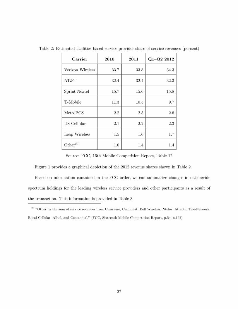
Table 2: Estimated facilities-based service provider share of service revenues (percent)

Carrier 2010 2011 Q1—Q2 2012

Verizon Wireless 33.7 33.8 34.3

AT&T 32.4 32.4 32.3

Sprint Nextel 15.7 15.6 15.8

T-Mobile 11.3 10.5 9.7

MetroPCS 2.2 2.5 2.6

US Cellular 2.1 2.2 2.3

Leap Wireless 1.5 1.6 1.7

Other20 1.0 1.4 1.4

Source: FCC, 16th Mobile Competition Report, Table 12

Figure 1 provides a graphical depiction of the 2012 revenue shares shown in Table 2.

Based on information contained in the FCC order, we can summarize changes in nationwide

spectrum holdings for the leading wireless service providers and other participants as a result of

the transaction. This information is provided in Table 3.

20“‘Other’ is the sum of service revenues from Clearwire, Cincinnati Bell Wireless, Ntelos, Atlantic Tele-Network,

Rural Cellular, Alltel, and Centennial.” (FCC, Sixteenth Mobile Competition Report, p.54, n.162)

27

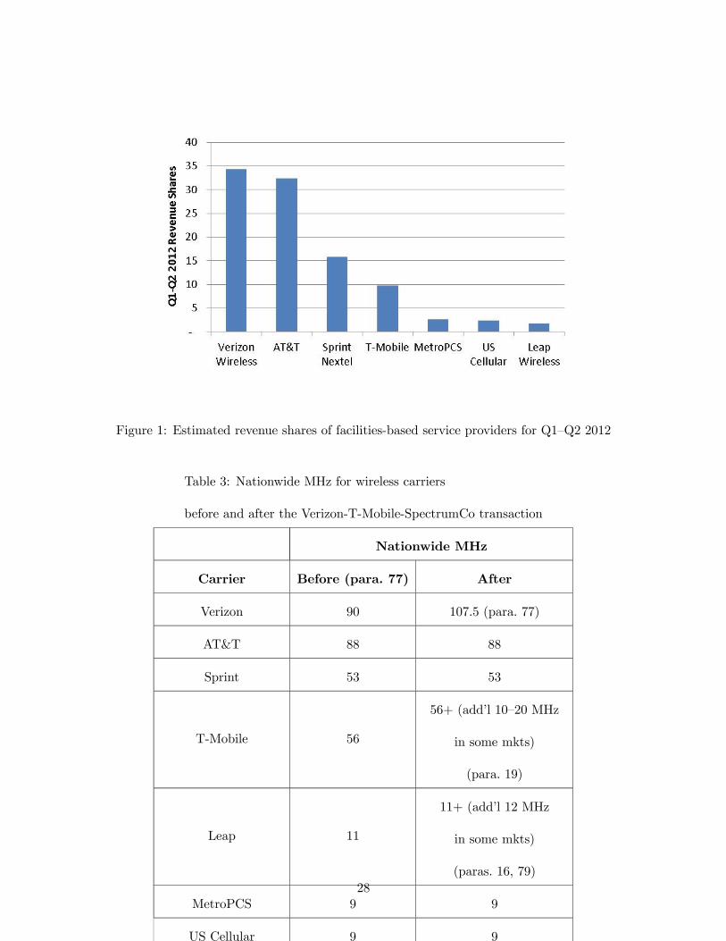
Figure 1: Estimated revenue shares of facilities-based service providers for Q1—Q2 2012

Table 3: Nationwide MHz for wireless carriers

before and after the Verizon-T-Mobile-SpectrumCo transaction

Nationwide MHz

Carrier Before (para. 77) After

Verizon 90 107.5 (para. 77)

AT&T 88 88

Sprint 53 53

T-Mobile 56

56+ (add’l 10—20 MHz

in some mkts)

(para. 19)

Leap 11

11+ (add’l 12 MHz

in some mkts)

(paras. 16, 79)

MetroPCS 9 9

US Cellular 9 9

28

For the purposes of this paper, we focus on the nationwide MHz of the four large carriers,

Verizon, AT&T, Sprint, and T-Mobile. Taking 20 MHz as the nationwide MHz sold by Cox and

SpectrumCo, and 17.5 MHz as the nationwide MHz gained by Verizon, we assume that T-Mobile’s

nationwide MHz increased by 2.5 MHz.

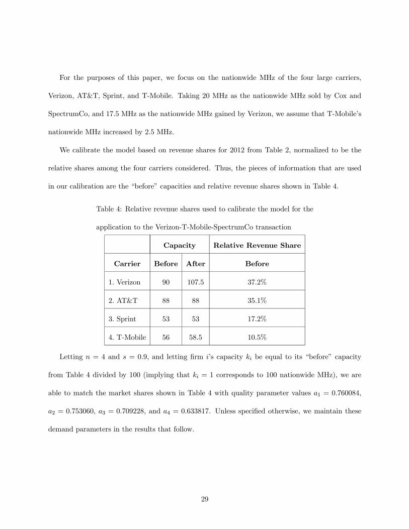
We calibrate the model based on revenue shares for 2012 from Table 2, normalized to be the

relative shares among the four carriers considered. Thus, the pieces of information that are used

in our calibration are the “before” capacities and relative revenue shares shown in Table 4.

Table 4: Relative revenue shares used to calibrate the model for the

application to the Verizon-T-Mobile-SpectrumCo transaction

Capacity Relative Revenue Share

Carrier Before After Before

1. Verizon 90 107.5 37.2%

2. AT&T 88 88 35.1%

3. Sprint 53 53 17.2%

4. T-Mobile 56 58.5 10.5%

Letting = 4 and = 09 and letting firm ’s capacity be equal to its “before” capacity

from Table 4 divided by 100 (implying that = 1 corresponds to 100 nationwide MHz), we are

able to match the market shares shown in Table 4 with quality parameter values 1 = 0760084,

2 = 0753060, 3 = 0709228, and 4 = 0633817. Unless specified otherwise, we maintain these

demand parameters in the results that follow.

29

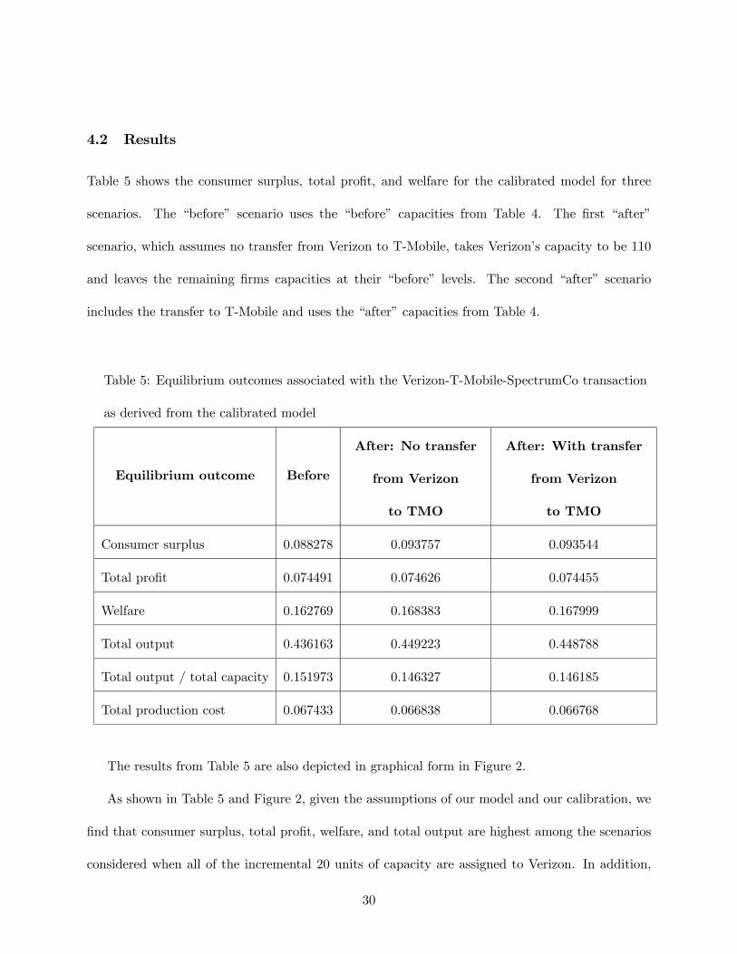
4.2 Results

Table 5 shows the consumer surplus, total profit, and welfare for the calibrated model for three

scenarios. The “before” scenario uses the “before” capacities from Table 4. The first “after”

scenario, which assumes no transfer from Verizon to T-Mobile, takes Verizon’s capacity to be 110

and leaves the remaining firms capacities at their “before” levels. The second “after” scenario

includes the transfer to T-Mobile and uses the “after” capacities from Table 4.

Table 5: Equilibrium outcomes associated with the Verizon-T-Mobile-SpectrumCo transaction

as derived from the calibrated model

Equilibrium outcome Before

After: No transfer

from Verizon

to TMO

After: With transfer

from Verizon

to TMO

Consumer surplus 0.088278 0.093757 0.093544

Total profit 0.074491 0.074626 0.074455

Welfare 0.162769 0.168383 0.167999

Total output 0.436163 0.449223 0.448788

Total output / total capacity 0.151973 0.146327 0.146185

Total production cost 0.067433 0.066838 0.066768

The results from Table 5 are also depicted in graphical form in Figure 2.

As shown in Table 5 and Figure 2, given the assumptions of our model and our calibration, we

find that consumer surplus, total profit, welfare, and total output are highest among the scenarios

considered when all of the incremental 20 units of capacity are assigned to Verizon. In addition,

30

 0.90 0.92 0.94 0.96 0.98 1.00 1.02 1.04 1.06 1.08

Before

After: No transfer fromVerizon to TMO

After: With transfer fromVerizon to TMO

Figure 2: Equilibrium outcomes associated with the Verizon-T-Mobile-SpectrumCo transaction as

derived from the calibrated model

Table 5 shows that at an aggregate level, output per unit capacity is higher when the incremental

units of capacity are assigned to Verizon rather than divided between Verizon and T-Mobile. Fi-

nally, even though total output increases as a result of the additional capacity, total product cost

decreases, with the decrease being slightly larger when the capacity is divided between Verizon and

T-Mobile. Table A.1 in the appendix provides firm-level details for the three scenarios.

As we explore these results further below, one must keep in mind that the results derive from

a model that assumes that market share differences among firms are explained by quality differ-

ences among firms. If, for example, the historical accumulation of market share, path dependence,

network effects, randomness, or other explanations account for market share differences, then our

results must be interpreted with that in mind. In addition, we have used a particular calibration

of the model for the purposes of this analysis, and other calibrations are possible.

31

In our model and calibration, assigning incremental spectrum to Verizon increases consumer

surplus and welfare, regardless of whether part of the spectrum is diverted to T-Mobile or not.

Verizon’s profit increases. T-Mobile’s profit is reduced in either scenario, although it is reduced

by less when it receives part of the additional spectrum. When T-Mobile is assigned spectrum,

its marginal cost is reduced; however, Verizon’s marginal cost is reduced as well and prices fall

sufficiently relative to the case without the additional spectrum that T-Mobile’s revenue and profits

decline.

Conditional on the simplified demand system we employ and simplifying assumptions on the

parameter values, our exercise shows that the market continues to be at the point where consumers

would benefit from assigning additional spectrum to Verizon (although, as shown below, the model

is capable of exhibiting the opposite behavior).

We also analyze the issue of warehousing within the context of our calibrated model using the

methods described in Section 3.2.4. As noted there, a firm’s output per unit of capacity decreases

when its capacity increases. Table A.1 in the appendix provides the detailed changes for the

scenarios we consider here.

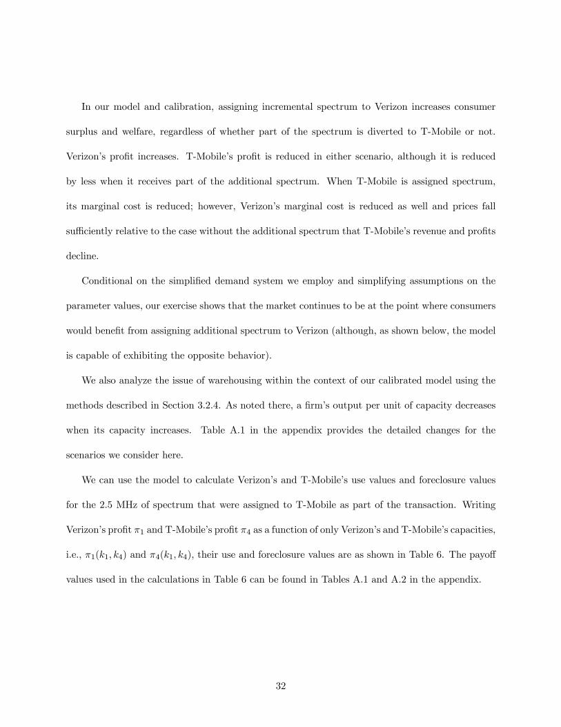
We can use the model to calculate Verizon’s and T-Mobile’s use values and foreclosure values

for the 2.5 MHz of spectrum that were assigned to T-Mobile as part of the transaction. Writing

Verizon’s profit 1 and T-Mobile’s profit 4 as a function of only Verizon’s and T-Mobile’s capacities,

i.e., 1(1 4) and 4(1 4) their use and foreclosure values are as shown in Table 6. The payoff

values used in the calculations in Table 6 can be found in Tables A.1 and A.2 in the appendix.

32

Table 6: Use and foreclosure values for the 2.5 MHz of spectrum that were assigned to T-Mobile

as part of the Verizon-T-Mobile-SpectrumCo transaction as derived from the calibrated model

Verizon T-Mobile

Use value

1(110 56)− 1(1075 56)

= 0031353− 0030952

= 0000401

4(1075 585)− 4(1075 56)

= 0007303− 0007069

= 0000234

Foreclosure value

1(1075 56)− 1(1075 585)

= 0030952− 0030777

= 0000175

4(1075 56)− 4(110 56)

= 0007069− 0006983

= 0000086

Total value 0000576 0000320

Foreclosure-share

measure of

warehousing

incentive

30% 27%

We also represent the values shown in Table 6 in Figure 3. These results show that based on

these measures Verizon’s use value for the spectrum is 71% greater than T-Mobile’s use value for

the spectrum. In addition, based on these measures, Verizon’s total value for the spectrum is 80%

greater than T-Mobile’s total value. Thus, the ranking of the total value and use values is aligned

in this case, suggesting that the market outcome would not be distorted by the issue of foreclosure

value.

Table 6 also shows the foreclosure-share measure of warehousing incentive. As shown there,

foreclosure value represents a similar share of total value for both Verizon and T-Mobile, which

33

Use

UseFore‐closure Fore‐

closure

Total

Total

0

0.0001

0.0002

0.0003

0.0004

0.0005

0.0006

Verizon T‐Mobile

Figure 3: Use and foreclosure values for the 2.5 MHz of spectrum that were assigned to T-Mobile

as part of the Verizon-T-Mobile-SpectrumCo transaction as derived from the calibrated model

reduces concerns that warehousing incentives might distort market outcomes.

Finally, we consider the excess-capacity measure of warehousing described in Section 3.2.4.

We illustrate the methodology by assuming that firms are endowed with a historical base level of

capacity, but that incremental units of capacity can be purchased through a competitive market.

For our illustration we assume that all firms are endowed with the same base level of capacity of

53, essentially using Sprint’s capacity as the normalization, and we assume that additional capacity

must be purchased in a competitive market at price . Letting k = (53 53) be the vector of base

capacities and k be the vector of additional capacity purchases, we calculate equilibrium capacity

levels ∗ () ≡ + () as a function of . Formally, we let () solve, for all

() ∈ argmax≥0

∗ (k + k)∗ (k

+ k)− (∗ (k + k) + )− .

34

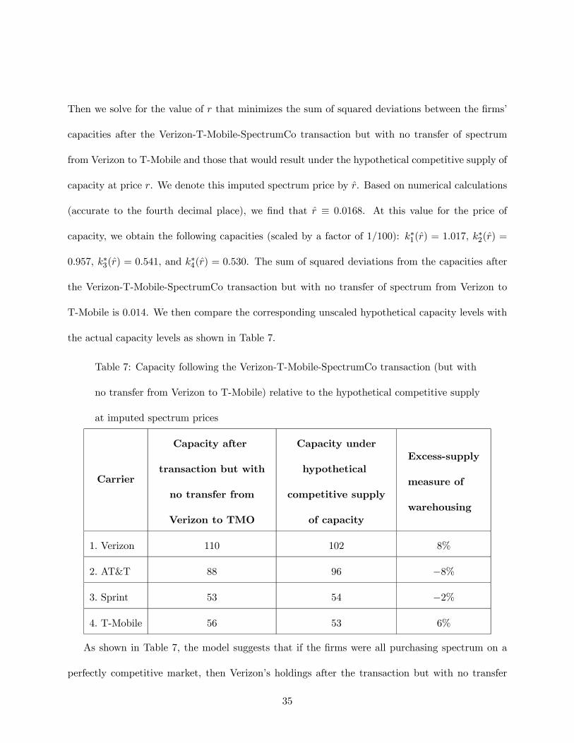
Then we solve for the value of that minimizes the sum of squared deviations between the firms’

capacities after the Verizon-T-Mobile-SpectrumCo transaction but with no transfer of spectrum

from Verizon to T-Mobile and those that would result under the hypothetical competitive supply of

capacity at price . We denote this imputed spectrum price by . Based on numerical calculations

(accurate to the fourth decimal place), we find that ≡ 00168. At this value for the price of

capacity, we obtain the following capacities (scaled by a factor of 1100): ∗1() = 1017, ∗2() =

0957, ∗3() = 0541, and ∗4() = 0530. The sum of squared deviations from the capacities after

the Verizon-T-Mobile-SpectrumCo transaction but with no transfer of spectrum from Verizon to

T-Mobile is 0014. We then compare the corresponding unscaled hypothetical capacity levels with

the actual capacity levels as shown in Table 7.

Table 7: Capacity following the Verizon-T-Mobile-SpectrumCo transaction (but with

no transfer from Verizon to T-Mobile) relative to the hypothetical competitive supply

at imputed spectrum prices

Carrier

Capacity after

transaction but with

no transfer from

Verizon to TMO

Capacity under

hypothetical

competitive supply

of capacity

Excess-supply

measure of

warehousing

1. Verizon 110 102 8%

2. AT&T 88 96 −8%

3. Sprint 53 54 −2%

4. T-Mobile 56 53 6%

As shown in Table 7, the model suggests that if the firms were all purchasing spectrum on a

perfectly competitive market, then Verizon’s holdings after the transaction but with no transfer

35

to T-Mobile would represent 8% more than the amount that would be expected, and T-Mobile’s

holdings would represent 6% more than the amount that would be expected. Of course, one must

interpret these results with caution given the underlying assumptions. However, if one were to

interpret these results within an overall framework that suggested that warehousing was likely

the greatest concern for Verizon and AT&T, and that T-Mobile is unlikely to be engaging in

significant warehousing, then these results would provide comfort that whatever concern there

might be regarding Verizon and AT&T is not substantial.

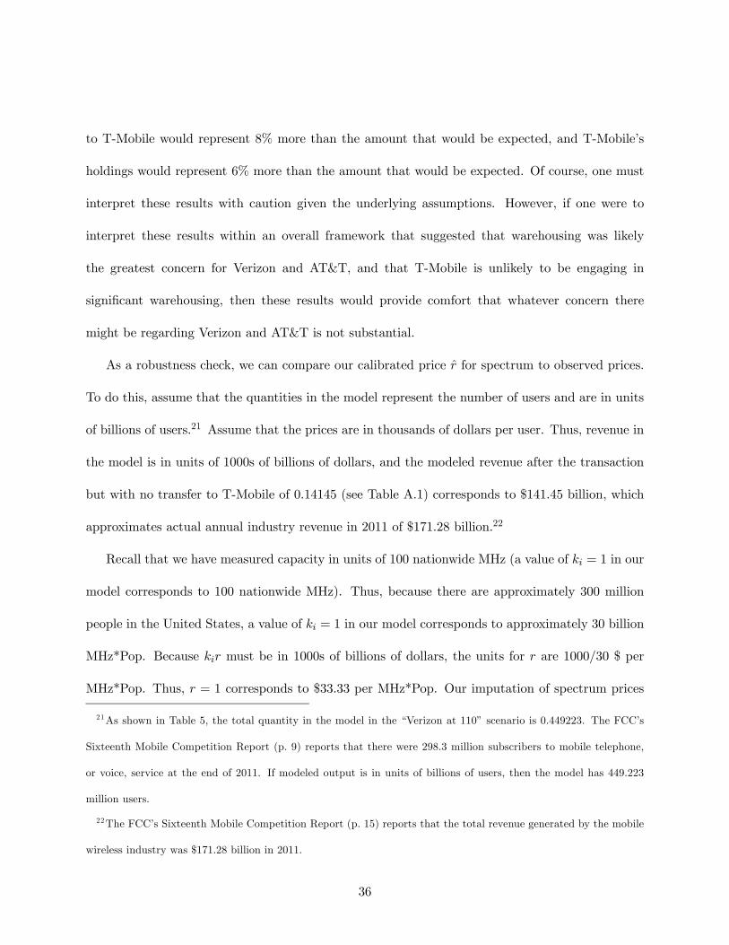
As a robustness check, we can compare our calibrated price for spectrum to observed prices.

To do this, assume that the quantities in the model represent the number of users and are in units

of billions of users.21 Assume that the prices are in thousands of dollars per user. Thus, revenue in

the model is in units of 1000s of billions of dollars, and the modeled revenue after the transaction

but with no transfer to T-Mobile of 0.14145 (see Table A.1) corresponds to $141.45 billion, which

approximates actual annual industry revenue in 2011 of $171.28 billion.22

Recall that we have measured capacity in units of 100 nationwide MHz (a value of = 1 in our

model corresponds to 100 nationwide MHz). Thus, because there are approximately 300 million

people in the United States, a value of = 1 in our model corresponds to approximately 30 billion

MHz*Pop. Because must be in 1000s of billions of dollars, the units for are 1000/30 $ per

MHz*Pop. Thus, = 1 corresponds to $33.33 per MHz*Pop. Our imputation of spectrum prices

21As shown in Table 5, the total quantity in the model in the “Verizon at 110” scenario is 0.449223. The FCC’s

Sixteenth Mobile Competition Report (p. 9) reports that there were 298.3 million subscribers to mobile telephone,

or voice, service at the end of 2011. If modeled output is in units of billions of users, then the model has 449.223

million users.

22The FCC’s Sixteenth Mobile Competition Report (p. 15) reports that the total revenue generated by the mobile

wireless industry was $171.28 billion in 2011.

36

delivered = 00168, which is 00168 ·3333 = 056 $/MHz*Pop.23 This price for capacity is similar

to the average price paid for AWS-1 spectrum in FCC auction 66, which was 0.53 $/MHz*Pop.24

The similarity of the price derived from our imputed with the actual price provides support for

the reasonableness of our calibration.

As an alternative approach, instead of imputing the hypothetical competitive price of capacity,

we can use the value of that corresponds to the observed price of $0.53 per MHz*Pop, which is

= 0533333 = 00159, then we obtain hypothetical capacity levels and excess-supply measure of

warehousing as shown in Table 8.

23To be more precise, let quantities be in units of (298.3 million / 0.449223 users) = 664 million users. Let

prices be in units of (171.28/0.14145 $billion / 664 million users) = 1820 $/per user. Then revenue is in units of

(17128014145 =) 1211 $billion. Since must be in 1211 $billion, the units for are 40.37 $/MHz*Pop. Thus,

= 1 corresponds to $40.37 per MHz*Pop, and = 00168 corresponds to 0.68 $/MHz*Pop.

24This calculation is based on FCC data, which are available at http://wireless.fcc.gov/auctions/default.htm?job=auction

_summary&id=66. Net winning bids were $13,700,267,150 and total MHz*Pops sold were 25,705,840,050.

37

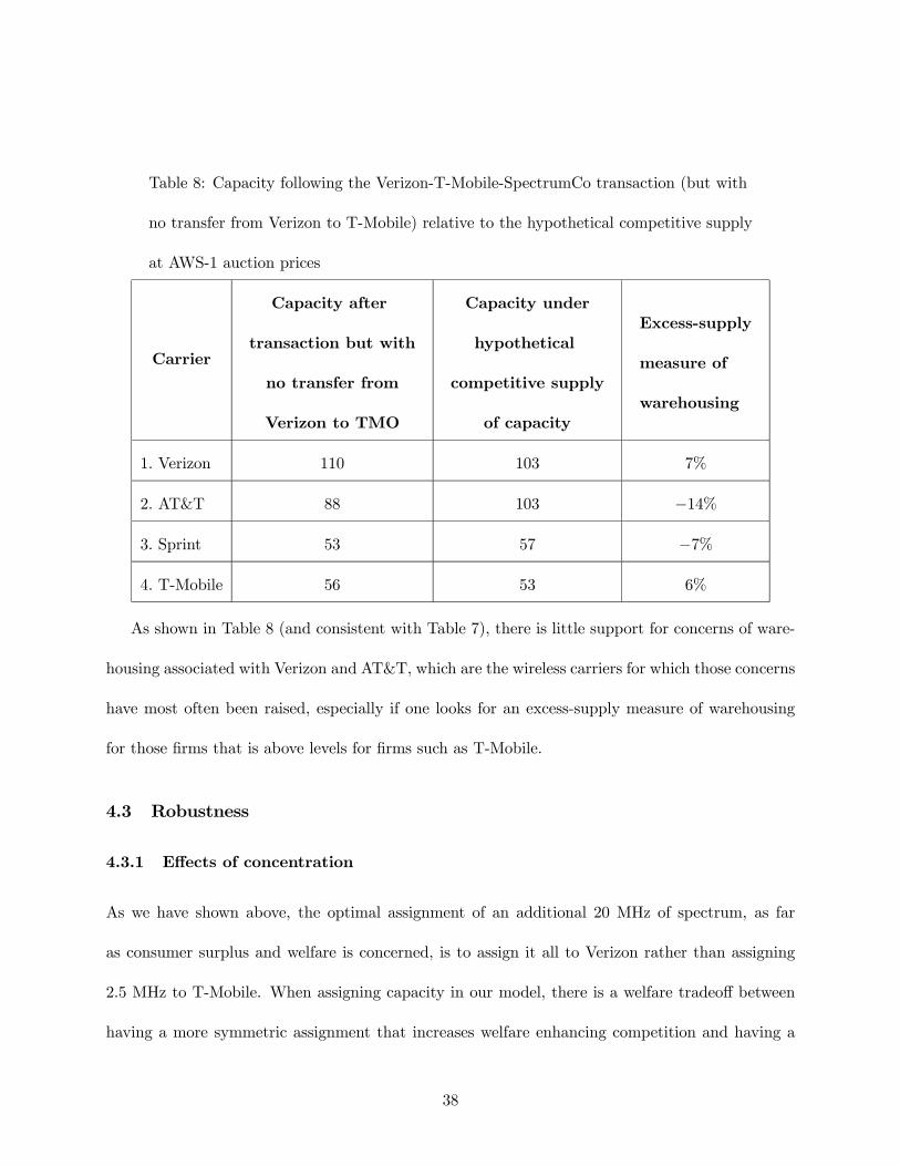
Table 8: Capacity following the Verizon-T-Mobile-SpectrumCo transaction (but with

no transfer from Verizon to T-Mobile) relative to the hypothetical competitive supply

at AWS-1 auction prices

Carrier

Capacity after

transaction but with

no transfer from

Verizon to TMO

Capacity under

hypothetical

competitive supply

of capacity

Excess-supply

measure of

warehousing

1. Verizon 110 103 7%

2. AT&T 88 103 −14%

3. Sprint 53 57 −7%

4. T-Mobile 56 53 6%

As shown in Table 8 (and consistent with Table 7), there is little support for concerns of ware-

housing associated with Verizon and AT&T, which are the wireless carriers for which those concerns

have most often been raised, especially if one looks for an excess-supply measure of warehousing

for those firms that is above levels for firms such as T-Mobile.

4.3 Robustness

4.3.1 Effects of concentration

As we have shown above, the optimal assignment of an additional 20 MHz of spectrum, as far

as consumer surplus and welfare is concerned, is to assign it all to Verizon rather than assigning

2.5 MHz to T-Mobile. When assigning capacity in our model, there is a welfare tradeoff between

having a more symmetric assignment that increases welfare enhancing competition and having a

38

more asymmetric assignment that increases welfare by favoring the firm that generates the most

value to consumers.25 In our calibration Verizon’s quality is sufficiently high that the value to

consumers from additional Verizon output outweighs the effects of increased concentration.

We now consider the extent to which this type of result continues to hold for larger assignments

of spectrum. In particular, we assume that there are additional units of spectrum to be distrib-

uted relative to the “before” capacities, and we consider the case in which −3 units are assigned

to Verizon and to each of the other three firms. Thus, = 4 corresponds to the assignment of

equal additional units of capacity to each of the four firms and = 0 corresponds to the assignment

of all of the additional units to Verizon.

Given our model and calibration, straightforward calculations show that for all integer values

of less than or equal to 150, consumer surplus is maximized at = 0: i.e., consumer surplus is

maximized when all of the additional spectrum is assigned to Verizon rather than an equal division

of some portion of that spectrum among the other three firms. However, for larger amounts

of spectrum, maximizing consumer surplus requires that not all of the spectrum be assigned to

Verizon.

In the calibration, the quality levels differ for the four firms, with Verizon having the highest

value of the quality parameter. Thus, consumer surplus is not maximized by having four equal-sized

firms. Maximizing consumer surplus requires assigning relatively more of the capacity to the firm

with the higher quality because that firm generates more value to consumers per unit of output.

25Additional effects are possible in models with increasing returns to scale technologies. For example, Horstmann

and Markusen (1986) show in a model of international trade with increasing returns to scale that protectionism can

reduce welfare by encouraging greater domestic firm entry and therefore lowering production levels (and increasing

costs) for individual firms.

39

Because we have assumed a simple linear demand formulation, one must use caution in interpreting

results, but under our formulation and calibration, consumers continue to benefit from assigning

additional capacity to Verizon rather than the alternatives we have considered for a substantial

range of increments to total capacity.

4.3.2 Calibration based on slopes

As a robustness check, we consider alternative assumptions about the demand system. Specifically,

we fix the quality parameters a = (1 4) = (1 1) and calibrate the model based on the slope

parameters b = (1 4), as opposed to the opposite approach considered above. We choose the

parameters b to minimize the sum of the squared deviations between actual and modeled revenue

shares.

Performing this exercise generates the following slope parameters (based on a search limited to

three decimal places): 1 = 0425, 2 = 0425, 3 = 0300, and 4 = 0975. Unlike the calibration

based on the quality parameters, where we are able to match the actual revenue shares essentially

exactly, in this calibration the sum of squared deviations for the revenue shares is 0.00001. Table

9 shows the actual and calibrated revenue shares.

Table 9: Calibrated revenue shares for a calibration based on slope parameters

Carrier Actual Relative Revenue Share Revenue Share in Calibrated Model

1. Verizon 37.2% 37.0%

2. AT&T 35.1% 35.5%

3. Sprint 17.2% 17.2%

4. T-Mobile 10.5% 10.5%

40

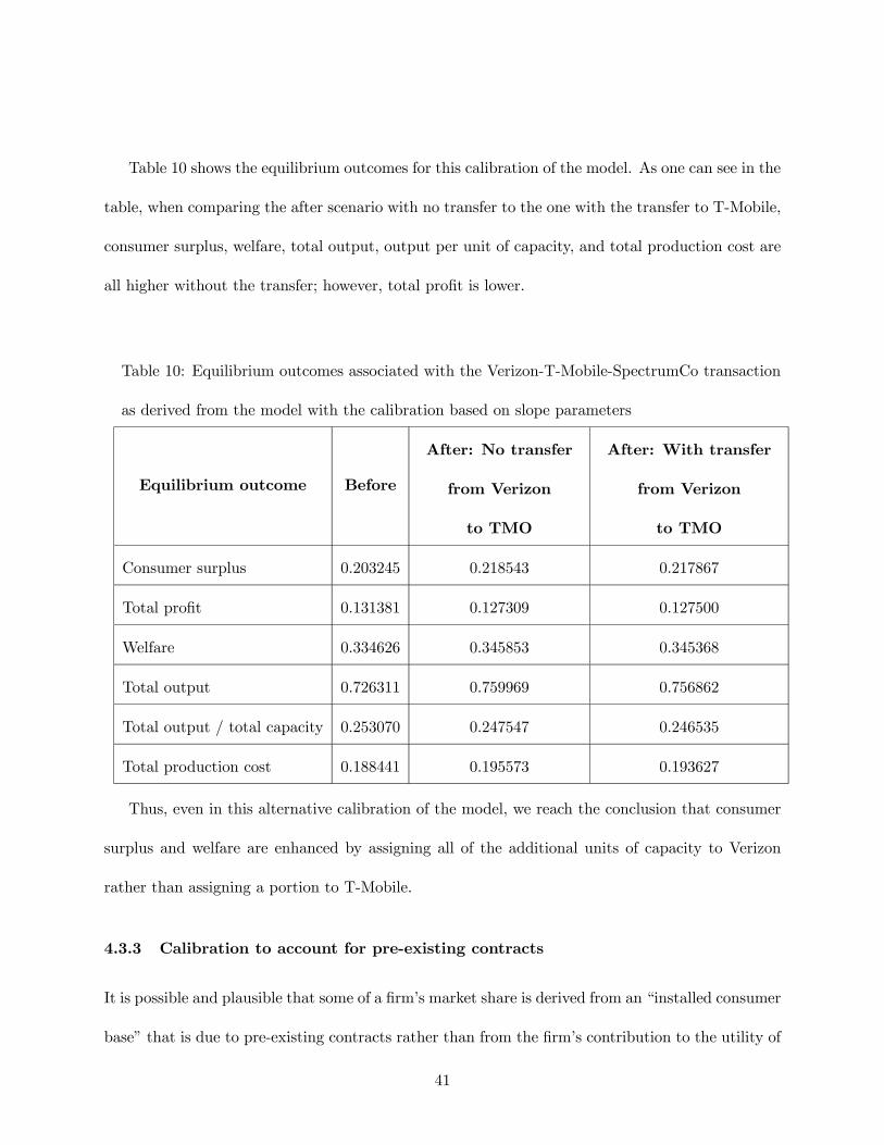
Table 10 shows the equilibrium outcomes for this calibration of the model. As one can see in the

table, when comparing the after scenario with no transfer to the one with the transfer to T-Mobile,

consumer surplus, welfare, total output, output per unit of capacity, and total production cost are

all higher without the transfer; however, total profit is lower.

Table 10: Equilibrium outcomes associated with the Verizon-T-Mobile-SpectrumCo transaction

as derived from the model with the calibration based on slope parameters

Equilibrium outcome Before

After: No transfer

from Verizon

to TMO

After: With transfer

from Verizon

to TMO

Consumer surplus 0.203245 0.218543 0.217867

Total profit 0.131381 0.127309 0.127500

Welfare 0.334626 0.345853 0.345368

Total output 0.726311 0.759969 0.756862

Total output / total capacity 0.253070 0.247547 0.246535

Total production cost 0.188441 0.195573 0.193627

Thus, even in this alternative calibration of the model, we reach the conclusion that consumer

surplus and welfare are enhanced by assigning all of the additional units of capacity to Verizon

rather than assigning a portion to T-Mobile.

4.3.3 Calibration to account for pre-existing contracts

It is possible and plausible that some of a firm’s market share is derived from an “installed consumer

base” that is due to pre-existing contracts rather than from the firm’s contribution to the utility of

41

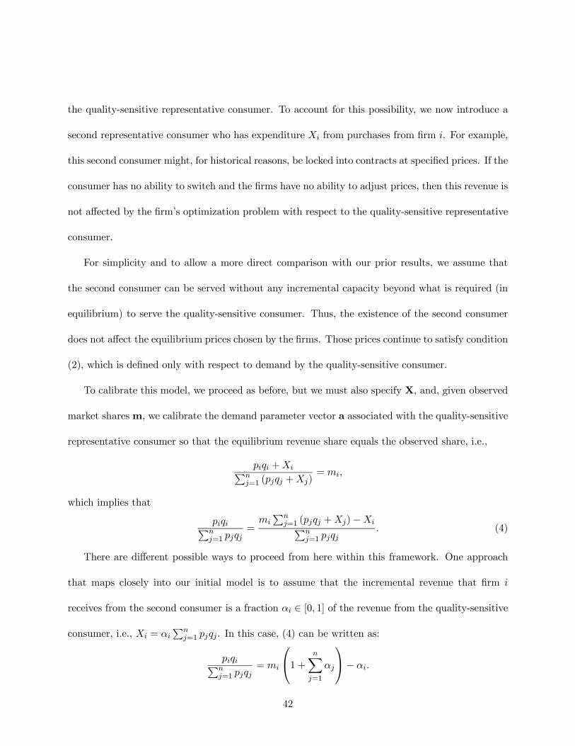
the quality-sensitive representative consumer. To account for this possibility, we now introduce a

second representative consumer who has expenditure from purchases from firm . For example,

this second consumer might, for historical reasons, be locked into contracts at specified prices. If the

consumer has no ability to switch and the firms have no ability to adjust prices, then this revenue is

not affected by the firm’s optimization problem with respect to the quality-sensitive representative

consumer.

For simplicity and to allow a more direct comparison with our prior results, we assume that

the second consumer can be served without any incremental capacity beyond what is required (in

equilibrium) to serve the quality-sensitive consumer. Thus, the existence of the second consumer

does not affect the equilibrium prices chosen by the firms. Those prices continue to satisfy condition

(2), which is defined only with respect to demand by the quality-sensitive consumer.

To calibrate this model, we proceed as before, but we must also specify X and, given observed

market sharesm, we calibrate the demand parameter vector a associated with the quality-sensitive

representative consumer so that the equilibrium revenue share equals the observed share, i.e.,

+P=1 ( +)

=

which implies that

P=1

=

P=1 ( +)−P

=1 (4)

There are different possible ways to proceed from here within this framework. One approach

that maps closely into our initial model is to assume that the incremental revenue that firm

receives from the second consumer is a fraction ∈ [0 1] of the revenue from the quality-sensitive

consumer, i.e., = P

=1 . In this case, (4) can be written as:

P=1

=

⎛⎝1 + X=1

⎞⎠−

42

Thus, to accommodate this extension, we need only calibrate the model to values for the market

shares that are adjusted for any pre-existing contracts that the firms have.

For example, if we assume that 10% of the revenue of Verizon and AT&T is due to such pre-

existing contracts, then instead of calibrating to the shares in Table 4, we would use the adjusted

shares that are shown in Table 11.

Table 11: Adjusted revenue shares used to calibrate the model

with a pre-existing contracts for Verizon and AT&T for the

application to the Verizon-T-Mobile-SpectrumCo transaction

pre-existing

contracts share

Capacity

Original

Revenue

Share

Adjusted

Revenue

Share

Carrier Before After

1. Verizon 10% 90 107.5 37.2% 34.6%

2. AT&T 10% 88 88 35.1% 32.1%

3. Sprint 0 53 53 17.2% 20.6%

4. T-Mobile 0 56 58.5 10.5% 12.6%

When we calibrate the model using the “before” capacities and the adjusted revenue shares

in Table 11, we get demand parameters 1 = 0735520, 2 = 0725902, 3 = 0727902, and 4 =

0646792. Comparing these to our prior results (reported following Table 4), we see that the use

of adjusted revenue shares results in lower quality parameters for Verizon and AT&T and higher

quality parameters for Sprint and T-Mobile.

Because the quality advantage for Verizon and AT&T is lower in this calibration, when we

recalculate the values for Table 5, we find that the welfare benefit from assigning all of the incre-

43

mental 20 units of capacity to Verizon is lower than under our original calibration, but they are

still positive. Details are provided in Table A.3 in the appendix.

In fact, if the share of pre-existing contracts for Verizon and AT&T increases to 35%, then

welfare is higher with the transfer of spectrum from Verizon to T-Mobile. If one views a 35%

share of pre-existing contracts as unlikely, then this supports the conclusion that, even if some

of Verizon’s market share is attributable to pre-existing rather than quality, it is unlikely to be

sufficient to overturn the result that welfare would be higher in the absence of the transfer of

spectrum to T-Mobile.

This extension of the model illustrates one way in which assumptions can be adjusted to account

for differences in firms’ market shares that may not be tied directly to quality differences. There are

different possibilities for how to approach this, which can be explored in future work. The option

we considered here illustrates the flexibility of the overall approach.

5 Conclusion

We provide an economic model that can be applied to competition among wireless service providers

that require access to spectrum in order to provide service. The model is one of price competition

among firms that offer differentiated products in which firms’ capacities (e.g., firms’ spectrum

license holdings) are fixed in the short-run and affect firms’ production costs, with higher capacity

resulting in a lower marginal cost.26

26The model, which is a slight generalization of the downstream market of the differentiated Bertrand model in

Loertscher and Reisinger (2014b), combines the demand side of Singh and Vives (1984) and Häckner (2000) with

a short-run cost function that represents constant returns to scale in the long-run, which has been used by Perry

(1978), Riordan (1998) and Loertscher and Reisinger (2014a).

44

The model is theoretically rich enough to capture the responses of market outcomes to changes

in the demand faced by competing wireless service providers and to changes in the allocation of

capacity. It also allows us to define two quantitative measures that can be used to assess the

extent that the “warehousing” of spectrum is a concern: Our first measure of warehousing — the

foreclosure-share measure of warehousing incentive — considers the difference between a firm’s use

value for an additional block of spectrum and its (theoretical) foreclosure value for that additional

block of spectrum. If a firm’s foreclosure value is low relative to its total value — particularly relative

to rivals — then warehousing incentives are weak. Our second measure of warehousing is the excess-

capacity measure of warehousing, which relates observed capacities with the equilibrium capacities

in a corresponding theoretical environment in which there is no incentive for warehousing. If actual

capacities exceed the capacities that would be expected in an environment with no warehousing

incentive, then that is suggestive of warehousing activity.

We analyze the Verizon-T-Mobile-SpectrumCo transaction of 2012 within the context of the

model by choosing parameters for the model so that the model’s outcomes are consistent with

actual pre-transaction revenue shares. Within the context of this calibration of our model, we find

that the Verizon-T-Mobile-SpectrumCo transaction increased consumer surplus and welfare, and

we find little evidence of warehousing motives for that transaction.

The analysis that we performed was limited by the availability of data and by a variety of

theoretical restrictions. For example, a more elaborate analysis would estimate rather than calibrate

the demand functions that give rise to the observed market shares. Nevertheless, we hope that the

model may prove useful for further research and applications. There is scope for deriving theoretical

measures of warehousing for more general models of capacity supply (e.g., the case of imperfectly

elastic supply) and eventually applying these in an analysis that explicitly estimates the demand

45

system rather than relying on calibration. Moreover, with good estimates of demand before and

after a merger, the model should also be useful in the analysis of the competitive effects of a

horizontal merger. The analysis offered here highlights the potential value of future empirical work

estimating demand for wireless markets.

46

A Appendix

Table A.1 provides firm-level details for the three scenarios described in Table 5.

Table A.1: Firm-level details of equilibrium outcomes for the three scenarios

that are associated with the Verizon-T-Mobile-SpectrumCo transaction as

derived from the calibrated model

Quantity Price Revenue Profit

Output per unit of

capacity

Verizon 0.14974 0.35256 0.05279 0.02787 0.16638

AT&T 0.14392 0.34612 0.04981 0.02627 0.16355

Sprint 0.07905 0.30877 0.02441 0.01261 0.14916

T-Mobile 0.06343 0.23492 0.01490 0.00771 0.11327

Verizon 0.17352 0.33843 0.05872 0.03135 0.15775

AT&T 0.13923 0.33483 0.04662 0.02459 0.15821

Sprint 0.07612 0.29731 0.02263 0.01169 0.14362

T-Mobile 0.06034 0.22348 0.01348 0.00698 0.10775

Verizon 0.17020 0.33915 0.05772 0.03077 0.15833

AT&T 0.13938 0.33521 0.04672 0.02464 0.15839

Sprint 0.07622 0.29769 0.02269 0.01172 0.14381

T-Mobile 0.06297 0.22361 0.01408 0.00730 0.10764

Panel (a): Details for the "before" scenario

Panel (b): Details for the "After: No transfer from Verizon to TMO" scenario

Panel (c): Details for the "After: With transfer from Verizon to TMO" scenario

Table A.2 provides firm-level details for the scenarios in which 2.5 MHz is transferred away from

Verizon but not allocated to any other bidder. This scenario is used in the calculation of use and

foreclosure values in Table 6.

47

Table A.2: Firm-level details of equilibrium outcomes for the case in which capacities are:

Verizon—107.5, AT&T—88, Sprint—53, and T-Mobile—56 using the calibrated model

Quantity Price Revenue Profit

Output per unit of

capacityVerizon 0.170689 0.340116 0.058054 0.030952 0.158781AT&T 0.139792 0.336182 0.046996 0.024789 0.158855Sprint 0.076473 0.298682 0.022841 0.011807 0.144288T-Mobile 0.060710 0.224840 0.013650 0.007069 0.108410

Table A.3 provides details related to the results in Section 4.3.3. The first row is the same as

the corresponding row in Table 5, while the second row provides the corresponding numbers for

the calibration that accounts for 10% pre-existing contracts.

Table A.3: Comparison of equilibrium welfare associated with the

Verizon-T-Mobile-SpectrumCo transaction as derived from the original

versus the adjusted calibration to allow for pre-existing contracts

Equilibrium

outcome

Before

After:

No

transfer

After:

With

transfer

Percentage

change from

no transfer

versus transfer

Welfare — original 0.162769 0.168383 0.167999 0.23%

Welfare — adjusted 0.157577 0.162611 0.162348 0.16%

48

Acknowledgements

We thank Michelle Connolly, Rosemary Humberstone, Federico Mini, Larry White, and participants

at the 2013 CMD workshop on spectrum economics at the University of Melbourne for valuable

comments.

References

Boccard, N. & Wauthy, X. (2000). Bertrand competition and Cournot outcomes: Further results.

Economics Letters, 68, 279—285.

Boccard, N. & Wauthy, X. (2004). Bertrand competition and Cournot outcomes: A correction.

Economics Letters, 84, 163—166.

Cave, J. & Salant, S. W. (1995). Cartel quotas under majority rule. American Economic Review,

85, 82—102.

Davidson, C. & Deneckere, R. A. (1986). Long-run competition in capacity, short-run competition

in price, and the Cournot model. RAND Journal of Economics, 17, 404—415.

Deneckere, R. A. & Kovenock, D. (1992). Price leadership. Review of Economic Studies, 59,

143—162.

Deneckere, R. A. & Kovenock, D. (1996). Bertrand-Edgeworth duopoly with unit cost asymmetry.

Economic Theory, 8, 1—25.

Edgeworth, F. Y. (1925). Papers relating to political economy: Volume I, the pure theory of

monopoly. London: Macmillan.

49

Esö, P., Nocke, V. & White, L. (2010). Competition for scarce resources. RAND Journal of

Economics, 41(3), 524—548.

Häckner, J. (2000). A note on price and quantity competition in differentiated oligopolies. Journal

of Economic Theory, 93(2), 233—239.

Horstmann, I. J. & Markusen, J. R. (1986). Up the average cost curve: Inefficient entry and the

new protectionism. Journal of International Economics, 20, 225—247.

Kreps, D. M. & Scheinkman, J. A. (1983). Quantity precommitment and Bertrand competition

yield Cournot outcomes. Bell Journal of Economics, 14, 326—337.

Levitan, R. E. & Shubik, M. (1972). Price duopoly and capacity constraints. International Eco-

nomic Review, 13, 111—122.

Loertscher, S. & Reisinger, M. (2014a). Market structure and the competitive effects of vertical

integration. RAND Journal of Economics (in press).

Loertscher, S. & Reisinger, M. (2014b). Market structure and the competitive effects of vertical

integration (January 30, 2014). Available at SSRN: http://ssrn.com/abstract=2388260 or

http://dx.doi.org/10.2139/ssrn.2388260.

Loertscher, S. (2008). Market making oligopoly. Journal of Industrial Economics, 56(2), 263—289.

Maggi, G. (1996). Strategic trade policies with endogenous mode of competition. American Eco-

nomic Review, 86(1), 237—258

Ordover, J. A., Saloner, G. & Salop, S. C. (1990). Equilibrium vertical foreclosure. American

Economic Review, 71, 127—142.

50

Perry, M. K. (1978). Vertical integration: The monopsony case. American Economic Review,

68(4), 561—570.

Riordan, M. H. (1998). Anticompetitive vertical integration by a dominant firm. American Eco-

nomic Review, 88, 1232—1248.

Shapiro, R. J., Holtz-Eakin, D. & Bazelon, C. (2013). The economic implications of restricting

spectrum purchases in the incentive auctions. Retrieved June 12, 2014, from Georgetown Uni-

versity Web site: http://www.gcbpp.org/files/Academic_Papers/EconImplicationsSpectrum

FINAL.pdf.

Singh, N. & Vives, X. (1984). Price and quantity competition in a differentiated duopoly. RAND

Journal of Economics, 15, 546—554.

Tirole, J. (1988). The theory of industrial organization. Cambridge, MA: MIT Press.

51