an oline data validation algorithm for electronic nose

AN OLINE DATA VALIDATION

ALGORITHM FOR ELECTRONIC NOSE

Mina Mirshahi

Vahid Partovi Nia

Luc Adjengue

June 2016

DS4DM-2016-002

POLYTECHNIQUE MONTRÉAL

DÉPARTEMENT DE MATHÉMATIQUES ET GÉNIE INDUSTRIEL

Pavillon André-Aisenstadt Succursale Centre-Ville C.P. 6079 Montréal - Québec H3C 3A7 Canada Téléphone: 514-340-5121 # 3314

An Online Data Validation Algorithm for ElectronicNose

Mina Mirshahi, Vahid Partovi Nia, and Luc Adjengue

Department of Mathematics and Industrial Engineering, Polytechnique Montreal, Montreal,Quebec, Canada

{mina.mirshahi,vahid.partovinia,luc.adjengue}@polymtl.cahttp://www.polymtl.ca

Abstract. An electronic nose (e-nose) is a device that analyzes the chemicalcomponents of an odour. The e-nose consists of an array of gas sensors for chem-ical detection, and a mechanism for pattern recognition to return the odour con-centration. Odour concentration defines the identifiability and perceivability ofan odour. Given that accurate prediction of odour concentration requires validmeasurements, automatic assessment of sampled measurements is of prime im-portance. The impairment of the e-nose, and environmental factors (includingwind, humidity, temperature, etc ) may introduce significant amount of noise. In-evitably, the pattern recognition results are affected. We propose an online algo-rithm to evaluate the validity of sensor measurements during the sampling beforeusing the data for pattern recognition phase. The proposed algorithm is computa-tionally efficient and straightforward to implement.

Keywords: Artificial olfaction, computational complexity, electronic nose, gassensor, outlier detection, robust covariance estimation.

An Online Data Validation Algorithm for ElectronicNose

Mina Mirshahi, Vahid Partovi Nia, and Luc Adjengue

Polytechnique Montreal

An Online Data Validation Algorithm for Electronic Nose 3

1 Introduction

1.1 Background

The recognition of chemicals in the environment is an essential need for the living or-ganisms. Odours are detected through millions of olfactory receptors that are locatedat the top of nasal cavities. The human olfactory system consists of three main compo-nents: 1) an array of olfactory receptors 2) the olfactory bulb that receives neural inputsabout odours detected by the receptors and 3) the brain. The olfactory system collectsa sample from its environment and transmit it to the brain, where it is recognized as aspecific odour.

An olfactory system is able to detect a broad range of smells. However, the hu-man olfacotry system fails to respond to many air pollutants; people can have differentsensitivity to many air pollutants and even be accustomed to toxic smells.

The contamination of air by harmful chemicals is referred to as air pollution andis one of the biggest concerns worldwide. This is mainly because the air pollution hasdirect influence on the environmental and human health. Auditing odourants is a cru-cial element in assessment of indoor and outdoor air quality. There are various odourmeasurement techniques such as dilution-to-threshold, olfactometers, and referencingtechniques (McGinley and Inc, 2002). The dependence of these methods on humanevaluation makes them less accurate and sometimes undesirable.

The concept of an artificial olfaction was introduced by Persaud and Dodd (1982).The primary artificial olfaction rely on a gas multisensor array. The term electronic nose(e-nose) appeared for the first time in the early 1990s (Gardner and Bartlett, 1994).E-nose is designed for recognizing simple or complex odours in its environment andit comprises two main elements of hardware and software. The hardware usually in-clude a set of gas sensors (such as metal oxide semi-conductors, conducting polymers,etc.) with partial specificity, air conditioner, flow controller, electronics, and many morecomponents. The software consists of statistical methods for pre-processing the dataand pattern recognition methods for predicting the odour concentration.

The gas sensors of e-nose should have certain features. Similar to human nose re-ceptors, the gas sensors of e-nose need to be highly sensitive with respect to chemi-cal compounds and less sensitive towards temperature and humidity. In addition, thesensors should be able to respond to various chemical compounds. Among the otherfeatures, one can name durability, selectivity, and easy calibration.

Gas sensor’s performance is affected by various elements. One of the most seriousdeterioration in sensors is owing to a phenomenon called drift. Drift is the low frequencychange in a sensor that causes offset measurements. Sensor drift, therefore, need to bedetected and compensated to guarantee accurate sensor measurments. Several methodshave been introduced to overcome the drift phenomenon including Carlo and Falasconi(2012); Artursson et al. (2000); Padilla et al. (2010); Zuppa et al. (2007).

The multivariate response of gas sensor arrays undergoes different pre-processingprocedures before the prediction is performed using statistical tools such as regres-sion, classification, or clustering. Gutierrez-Osuna (2002); Kermiti and Tomic (2003);Bermak et al. (2006) have discussed methods for analyzing the gas sensor array data.

4 Mina Mirshahi, Vahid Partovi Nia, and Luc Adjengue

1.2 Motivation

The e-nose is capable of reproducing the human sense of smell using an array of gassensors and pattern recognition methods. Pattern recognition methods use a set of la-belled data to predict the odour concentration for each set of sensor measurements. Thelabelled data consist of a sub-sample of sensors’ outputs considered for further analysesof its concentration in olfactometry.

One of the application of e-nose is in environmental activities; e-noses provide in-dustries with odour management plan to minimize the effect of odour in the environ-ment. To this end, e-noses are installed in outdoor fields such as compost sites, landfillsites, waste water plants, etc., where the environmental condition can greatly fluctuate.Consequently, the occurrence of unwanted variability is very typical.

During the sampling process, sensors in the e-nose device may report incorrect val-ues or some of the sensors stop functioning for a short period of time. These anomaliesare ought to be diagnosed and reported in real time using a computationally efficientalgorithm, which is the focus of this research.

We propose an online data validation algorithm which compares e-nose measure-ments with a set of reference samples and allocate them accordingly to different zones.The zones are distinguished from each other using distinct colors like green, yellow,red, etc., to represent the extent of the validity of the measurement. The main focus ofthis work is summarized in the flowchart below.

Start

Require the e-nosemeasurements.

Pre-processthe data.

Perform datavalidation.

Predict the odourconcentration.

Require thereference sets.

Stop

Return the zone assignment(Green, Yellow, Red, etc.).

Return the odourconcentration prediction.

Fig. 1: A schematic flowchart of the proposed online task for an e-nose.


1.3 Data Preparation

The e-nose relies on a sensor array consists of several gas sensors. The number of thesensors depends on the purpose of analysis. Each sensor represents an attribute; themore the sensors are, the better the e-nose discriminate among analytes. Nonethelessthe inclusion of too many sensors can lead to unnecessary data and a complex system.

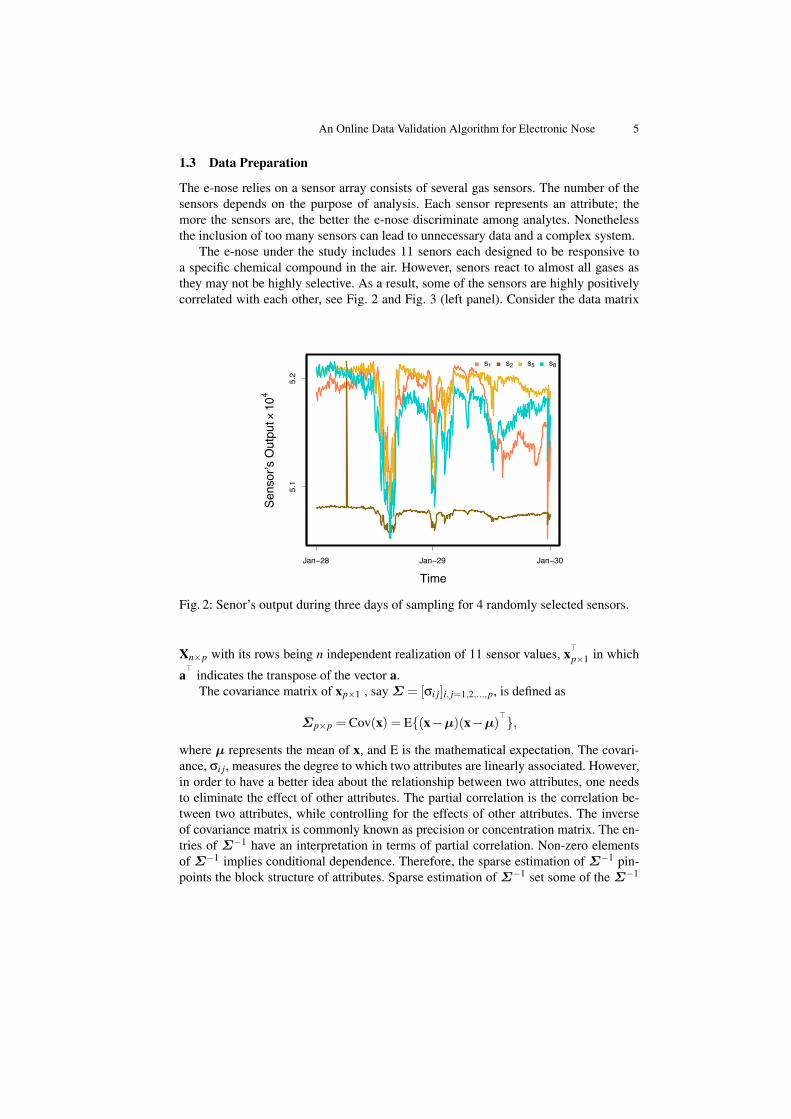
The e-nose under the study includes 11 senors each designed to be responsive toa specific chemical compound in the air. However, senors react to almost all gases asthey may not be highly selective. As a result, some of the sensors are highly positivelycorrelated with each other, see Fig. 2 and Fig. 3 (left panel). Consider the data matrix

Time

Sens

or’s

Out

put×

104

Jan−28 Jan−29 Jan−30

5.1

5.2

s1 s2 s5 s8

Fig. 2: Senor’s output during three days of sampling for 4 randomly selected sensors.

Xn×p with its rows being n independent realization of 11 sensor values, x>p×1 in which

a> indicates the transpose of the vector a.The covariance matrix of xp×1 , say Σ = [σi j]i, j=1,2,...,p, is defined as

Σp×p = Cov(x) = E{(x−µ)(x−µ)>},

where µ represents the mean of x, and E is the mathematical expectation. The covari-ance, σi j, measures the degree to which two attributes are linearly associated. However,in order to have a better idea about the relationship between two attributes, one needsto eliminate the effect of other attributes. The partial correlation is the correlation be-tween two attributes, while controlling for the effects of other attributes. The inverseof covariance matrix is commonly known as precision or concentration matrix. The en-tries of Σ−1 have an interpretation in terms of partial correlation. Non-zero elementsof Σ−1 implies conditional dependence. Therefore, the sparse estimation of Σ−1 pin-points the block structure of attributes. Sparse estimation of Σ−1 set some of the Σ−1


entries to zero. Investigation of the inherent dependence between the sensor values isthen performed by means of the partial correlation.

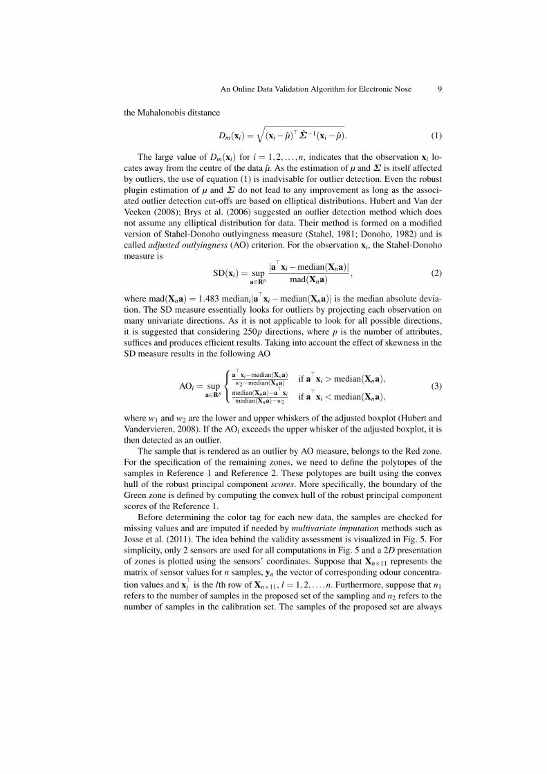
Here, the graphical lasso (Friedman et al., 2008) is considered for a better under-standing of the existing relationship between the sensor values. Friedman et al. (2008)proposed estimating the covariance matrix such that its inverse, Σ−1, is sparse by ap-plying a lasso penalty (Tibshirani, 1996). In Fig. 3 (right panel), the undirected graphconnects two attributes which are conditionally correlated given all other attributes. Thesensors 5 to 8 are correlated with each other conditioning on the effect of the others.This is also reflected in the heatmap of the correlation matrix Fig. 3 (left panel). This de-pendence must be taken into account while modelling the data. Gaussianity of the datais another crucial assumption that should be verified. The validity of this assumptionfor the sensor values is tested using various methods such as analyzing the distributionof individual sensor values, scatter plot of the linear projection of data using principalcomponents, estimating the multivariate kurtosis and skewness, and also multivariateMardia test, see Fig. 4.

2 Data Analysis

We aim to verify the validity of e-nose measurements by considering some referencesamples for the purpose of comparison. These reference samples are collected whenthe e-nose functions normally, and the conditions are fully under control. The e-nosemeasurements are compared with reference samples and are allocated to various zonesaccordingly. These zones are distinguished by various colors, like green, yellow, red,etc., to indicate the status of e-nose measurements (Mirshahi et al., 2016).

Two distinct reference sets, if applicable, are recommended for data validation. Ref-erence 1 consists of data in a period of sampling defined by an expert after installationof the e-nose. The data in this period of sampling is called as proposed set. Reference 2,upon its availability, is manually gathered samples from the field that are brought tothe laboratory for quantification of their odour concentration. The data in this periodof sampling is called calibration set, to emphasize that it can be incorporated for datamodelling using a supervised learning algorithm.

If a new datum does not follow the overall pattern of data previously observed, thenit is marked as an outlier and is assigned to Red zone. This zone represents a dramaticchange in the pattern of samples and is referred to as “risky” observations. If the newdatum is not an outlier and it is also located within the data polytope of the Reference 1or the Reference 2, it is allocated to Green or Blue zone respectively. These zonesrepresent the “safe” observations. If the new datum is not an outlier, but outside of thearea of Green and Blue zones, they are assigned to Yellow zone. This zone displayspotentially “critical” observations.

If large proportion of samples belong to the Yellow and Red zones, the reliabilityof the system should be suspected. Undesirable measurements can be the outcome ofphysical complications, such as sensor loss in the e-nose, or sudden changes in thechemical pattern of the environment. Zone assignment, therefore, require some outlierdetection algorithms. For the Green and the Blue zones, the new samples are projectedonto a subspace with lower dimension. Dimension reduction methods such as principal


s 11

s 9s 7

s 5s 3

s 1

s1 s3 s5 s7 s9 s110

0.1

0.2

0.3

0.4

0.5

0.6

0.7

0.8

0.9

1

s1

s2

s3s4s5

s6

s7

s8s9 s10

s11

Fig. 3: Left panel, heatmap of the correlation matrix of the sensor values (s1–s11). Rightpanel, the undirected graph of partial correlation using the graphical lasso. The undi-rected graph of the right panel approves the block structure of the heatmap of the leftpanel.

0 200 400 600 800 1000

1020

3040

Squared Mahalanobis Distance

Chi−S

quar

e Q

uant

ile

×10

−4

35 40 45 50

02

46

s1 × 103

Density

×10

−4

35 40 45 50

02

46

s6 × 103

Density

×10

−4

35 40 45 50

02

46

s11 × 103

Density

Fig. 4: Left panel, the Q-Q plot of squared Mahalanobis distance supposed to follow thechi-squared distribution for Gaussian data. Right panel, the marginal density for somerandomly chosen sensor values. Both graphs confirm the non-Gaussianity of data.


44 48 52

3637

3839

s1 × 103

s 2×10

3

0

0.5

1

1.5

2

×10

−7

Fig. 5: Validity assessment for about 700 samples based on 2 sensor values. Left panel,the plot illustrates the contour map of estimated density function for the 2 sensors. Rightpanel, the density function of the samples demonstrated in 3D with zones identified foreach of the samples in the sensor 1 (s1) versus sensor 2 (s2) plane. Higher density isassigned to the Green, Blue, and Orange zones compared to the Yellow and Red zones.

component analysis (PCA) can serve for this purpose (Jolliffe, 2002). PCA attemptsto explain the data covariance matrix, Σ̂, by a set of components; these componentsare the linear combination of the primary attributes. PCA, basically, converts a set ofpossibly correlated attributes into a set of linearly uncorrelated axes through orthogonallinear transformations. The first k (k < p) principal components are the eigenvectorsof the covariance matrix Σ associated with the k largest eigenvalues. The classicalestimation of covariance matrix, Σ̂, is strongly influenced by outliers (Prendergast,2008). As producing outlier is typical of sensor data, robust covariance estimation mustbe applied to avoid misleading results.

Robust principal component analysis (Hubert et al., 2005) is employed for dimen-sion reduction purpose throughout this article. This robust PCA computes the covari-ance matrix through projection pursuit (Li and Chen, 1985) and minimum covariancedeterminant (Croux and Haesbroeck, 2000) methods. The robust PCA procedure can besummarized as follows:

1. The matrix of data is pre-processed such that the data spread in the subspace of atmost min(n−1, p).

2. In the spanned subspace, the most obvious outliers are diagnosed and removed fromdata. The covariance matrix is calculated for the remaining data, Σ̂0.

3. Σ̂0 is used to decide about the number of principal components to be retained inthe analysis, say k0 (k0 < p).

4. The data are projected onto the subspace spanned by the first k0 eigenvectors ofΣ̂0.

5. The covariance matrix of the projected points is estimated robustly using minimumcovariance determinant method and its k leading eigenvalues are computed. Thecorresponding eigenvectors are the robust principal components.

The Red zone represents the outliers of the samples as being measured by the e-nosethrough time. One common approach for detecting outliers in multivariate data is to use


the Mahalonobis ditstance

Dm(xi) =

√(xi− µ̂)>Σ̂−1(xi− µ̂). (1)

The large value of Dm(xi) for i = 1,2, . . . ,n, indicates that the observation xi lo-cates away from the centre of the data µ̂. As the estimation of µ and Σ is itself affectedby outliers, the use of equation (1) is inadvisable for outlier detection. Even the robustplugin estimation of µ and Σ do not lead to any improvement as long as the associ-ated outlier detection cut-offs are based on elliptical distributions. Hubert and Van derVeeken (2008); Brys et al. (2006) suggested an outlier detection method which doesnot assume any elliptical distribution for data. Their method is formed on a modifiedversion of Stahel-Donoho outlyingness measure (Stahel, 1981; Donoho, 1982) and iscalled adjusted outlyingness (AO) criterion. For the observation xi, the Stahel-Donohomeasure is

SD(xi) = supa∈Rp

|a>xi−median(Xna)|mad(Xna)

, (2)

where mad(Xna) = 1.483 mediani|a>xi−median(Xna)| is the median absolute devia-

tion. The SD measure essentially looks for outliers by projecting each observation onmany univariate directions. As it is not applicable to look for all possible directions,it is suggested that considering 250p directions, where p is the number of attributes,suffices and produces efficient results. Taking into account the effect of skewness in theSD measure results in the following AO

AOi = supa∈Rp

a>

xi−median(Xna)w2−median(Xna) if a>xi > median(Xna),

median(Xna)−a>

ximedian(Xna)−w2

if a>xi < median(Xna),(3)

where w1 and w2 are the lower and upper whiskers of the adjusted boxplot (Hubert andVandervieren, 2008). If the AOi exceeds the upper whisker of the adjusted boxplot, it isthen detected as an outlier.

The sample that is rendered as an outlier by AO measure, belongs to the Red zone.For the specification of the remaining zones, we need to define the polytopes of thesamples in Reference 1 and Reference 2. These polytopes are built using the convexhull of the robust principal component scores. More specifically, the boundary of theGreen zone is defined by computing the convex hull of the robust principal componentscores of the Reference 1.

Before determining the color tag for each new data, the samples are checked formissing values and are imputed if needed by multivariate imputation methods such asJosse et al. (2011). The idea behind the validity assessment is visualized in Fig. 5. Forsimplicity, only 2 sensors are used for all computations in Fig. 5 and a 2D presentationof zones is plotted using the sensors’ coordinates. Suppose that Xn×11 represents thematrix of sensor values for n samples, yn the vector of corresponding odour concentra-tion values and x>l is the lth row of Xn×11, l = 1,2, . . . ,n. Furthermore, suppose that n1refers to the number of samples in the proposed set of the sampling and n2 refers to thenumber of samples in the calibration set. The samples of the proposed set are always


available, but not necessarily the calibration set. Two different scenarios occur based onthe availability of the calibration set.

If the calibration set is accessible, then Scenario 1 happens. Otherwise, we onlydeal with Scenario 2. Scenario 1 is a general case which is explained more in detail.The data undergo a pre-processing stage, including imputation and outlier detection,before any further analyses. Having done the pre-processing stage, data are stored asReference 1, Xn1×11, and Reference 2, Xn2×11. The first k, e.g. k = 2,3, robust principalcomponents of Xn1×11 are calculated and the corresponding loading matrix is denotedby L1. The pseudo code of two algorithms for Scenario 1 is provided below. Scenario2 is a special case of Scenario 1 in which Sub-Algorithm (Scenario 1) is used withConvexHull(2) = ∅ that eliminates the Blue and Orange zones. Consequently, there isno model for odour concentration prediction in the Main Algorithm.

Sub-Algorithm (Scenario 1)

1: if the point x>l , l = 1,2, . . . ,N is identified as an outlier by AO measure then2: x>l is in Red zone,3: else if x>l L1 ∈ ConvexHull(1) AND x>l L1 6∈ ConvexHull(2) then4: x>l is in Green zone,5: else if x>l L1 6∈ ConvexHull(1) AND x>l L1 ∈ ConvexHull(2) then6: x>l is in Blue zone,7: else if x>l L1 ∈ ConvexHull(1) AND x>l L1 ∈ ConvexHull(2) then8: x>l is in Orange zone,9: else

10: x>l is in Yellow zone.11: end if

Main Algorithm (Scenario 1)Require: Xn1×11, Xn2×11, and the loading matrix L1 using robust PCA over Reference 1,

Xn1×11.1: ConvexHull(1) ← the convex hull of the projected values of the Reference 1, Xn1×11L1.2: Train a supervised learning model on Reference 2, Xn2×11, and its odour concentration vec-

tor, yn2 .3: ConvexHull(2) ← the convex hull of the projected values of the Reference 2, Xn2×11L1.4: Do Sub-Algorithm for new data x∗.5: Predict the odour concentration for new data x∗ using the trained supervised learning model.

In Section 3, a set of simulated data is used to verify the relevancy of our proposedalgorithm and the choice of statistical methods. The applicability of our algorithm isalso tested based on 8 months sampling from the e-nose in Section 4.


3 Simulation

We examine the methodology on two sets of simulated data to highlight the importanceof the assumptions such as non-elliptical contoured distribution and robust estimationconsidered in our methodology. In each example, we stored the simulated data in thematrix Xn×2, where x>l = (xl1,xl2); l = 1,2, . . . ,n.

In the first example, the data is simulated from a mixture distribution with 10% con-tamination. The elements of mixture distribution are chosen arbitrarily from Gaussianand the Student’s t-distribution.

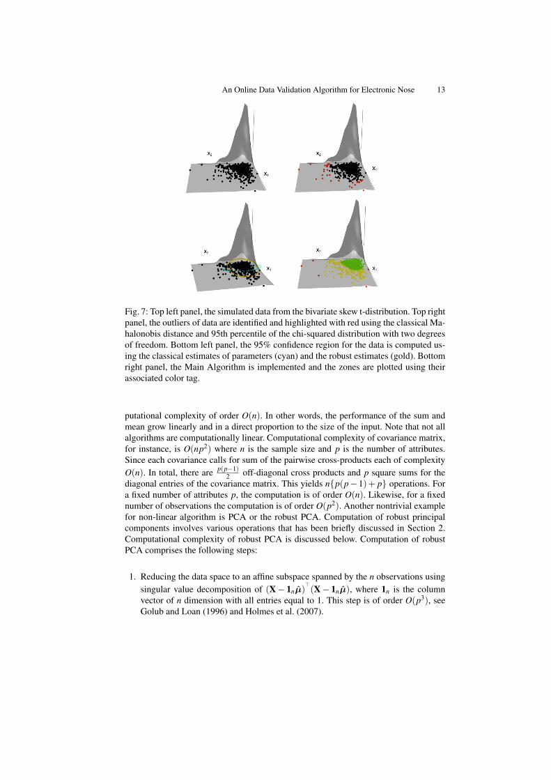
We simulated data from the bivariate skew t-distribution (Gupta, 2003) in the secondexample in order to test the effect of skewness on our algorithm, .

Using classical approaches for outlier detection without considering the actual datadistribution, mistakenly renders many observations as outliers, Fig. 6 and Fig. 7 (topright panel). The parameters of interest, the mean vector and the covariance matrix,need to be estimated robustly, otherwise the confidence region misrepresents the un-derlying distribution. In Fig. 6 and Fig. 7 (bottom left panel), the classical confidenceregion is pulled toward the outlier observations. On the contrary, the robust confidenceregion perfectly unveil the distribution of the majority of observations because of therobust and efficient estimation of the mean and the covariance matrix. Consequently, theclassical principal components are affected by the inefficient estimation of the covari-ance matrix. We proposed using methods that deal with asymmetric data appropriately.Adjusted outlyingness (AO) measure identifies the outliers of the data correctly. Con-sidering a sub-sample of data as Reference 1 in each of the examples, the result of theMain Algorithm can be observed in the right bottom panel of Fig. 6 and Fig. 7.

4 Experiment

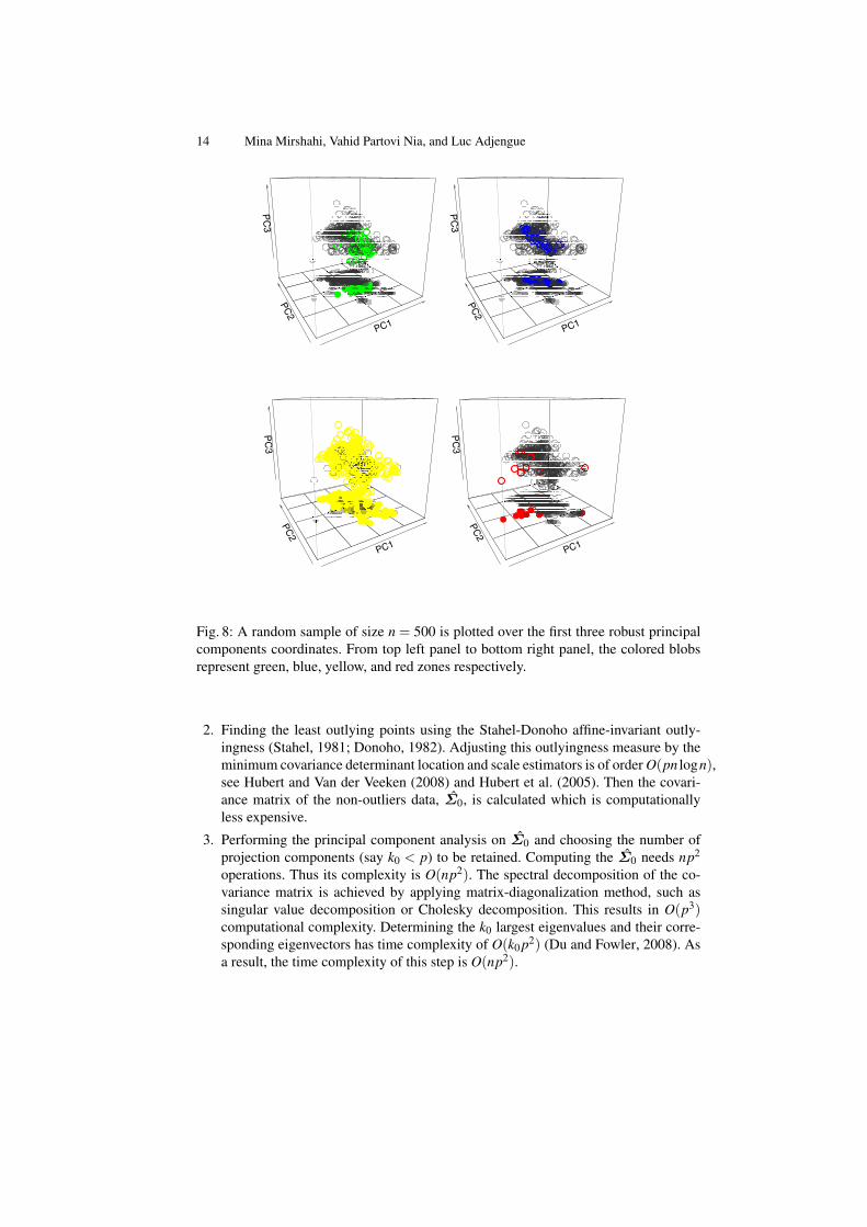
In order to evaluate the performance of our data validation method, we implement theMain Algorithm on a collection of e-nose measurements. We decide to keep the the first3 robust principle components of the data PC1, PC2, PC3 for simplification and the easyvisualization. The 3 principal components correspond to the 3 largest eigenvalues of therobust covariance matrix. Prior to the implementation of the Main Algorithm, the dataundergoes a pre-processing stage including the imputation of the missing values.

The validity of the e-nose measurements are identified using the Main Algorithmfor the 8 months of sampling. In favor of more readable graphs, only a subset of 500samples out of 200 thousands of observations are plotted. In Fig. 8, the sample points aredrawn in gray and each zone is highlighted using its corresponding color. The circles inFig. 8 are also illustrated on PC1 and PC2 plane for a better demonstration of the zones.

The interpretation of a zones is heavily depends on its definition. For instance, theGreen, Blue, and Orange zones, represent samples that are very close the samples thathave already been observed in either Reference 1 or Reference 2. As the observations inreference sets were entirely under control, the Green, Blue, and Orange zones affirm thevalidity of the samples. In addition, the accuracy of the gas concentration predicted forthese zones is certified. On the other hand, the gas concentration prediction for samples


Fig. 6: Top left panel, the simulated data from the mixture distribution f (x) = (1−ε) f1(x) + ε f2(x) with contamination proportion of ε = 1

10 , and f1 and f2 being theGaussian and Student’s t-distribution respectively. Top right panel, the outliers of dataare identified and highlighted with red using the classical Mahalonobis distance and95th percentile of the chi-squared distribution with two degrees of freedom. Bottom leftpanel, the 95% confidence region for the data is computed using the classical estimatesof parameters (cyan) and the robust estimates (gold). Bottom right panel, the MainAlgorithm is implemented and the zones are plotted using their associated color tag.

in the Red zone is less accurate compared with that of the Green, Blue, and Orangezones.

The data that are significantly dissimilar to the already observed data deserve fur-ther attention. These data are outliers and are reported in the Red zone. Similarly, thegas concentration predictions associated with samples in the Red zone can be very mis-leading. Generating a remarkable percentage of samples belonging to the Yellow andthe Red zones refers to the possible failure of the e-nose equipment.

5 Computational Complexity

Here, we discuss the computational complexity of our proposed algorithm (Main Algo-rithm). First, a brief introduction to computational complexity is given to facilitate theunderstanding.

The computational complexity of an algorithm is studied asymptotically by the bigO-notation (Arora and Barak, 2009). The big O-notation explains how quickly the run-time of an algorithm grows relative to its input. For instance, sum of n values require(n−1) operations. Consequently, the mean requires n operations reserving one for thedivision of the sum by n. As they are both bounded by a linear function, they have com-


Fig. 7: Top left panel, the simulated data from the bivariate skew t-distribution. Top rightpanel, the outliers of data are identified and highlighted with red using the classical Ma-halonobis distance and 95th percentile of the chi-squared distribution with two degreesof freedom. Bottom left panel, the 95% confidence region for the data is computed us-ing the classical estimates of parameters (cyan) and the robust estimates (gold). Bottomright panel, the Main Algorithm is implemented and the zones are plotted using theirassociated color tag.

putational complexity of order O(n). In other words, the performance of the sum andmean grow linearly and in a direct proportion to the size of the input. Note that not allalgorithms are computationally linear. Computational complexity of covariance matrix,for instance, is O(np2) where n is the sample size and p is the number of attributes.Since each covariance calls for sum of the pairwise cross-products each of complexityO(n). In total, there are p(p−1)

2 off-diagonal cross products and p square sums for thediagonal entries of the covariance matrix. This yields n{p(p−1)+ p} operations. Fora fixed number of attributes p, the computation is of order O(n). Likewise, for a fixednumber of observations the computation is of order O(p2). Another nontrivial examplefor non-linear algorithm is PCA or the robust PCA. Computation of robust principalcomponents involves various operations that has been briefly discussed in Section 2.Computational complexity of robust PCA is discussed below. Computation of robustPCA comprises the following steps:

1. Reducing the data space to an affine subspace spanned by the n observations usingsingular value decomposition of (X− 1nµ̂)

>(X− 1nµ̂), where 1n is the column

vector of n dimension with all entries equal to 1. This step is of order O(p3), seeGolub and Loan (1996) and Holmes et al. (2007).


PC1

PC2

PC3

PC1

PC2

PC3

PC1

PC2

PC3

PC1

PC2

PC3

Fig. 8: A random sample of size n = 500 is plotted over the first three robust principalcomponents coordinates. From top left panel to bottom right panel, the colored blobsrepresent green, blue, yellow, and red zones respectively.

2. Finding the least outlying points using the Stahel-Donoho affine-invariant outly-ingness (Stahel, 1981; Donoho, 1982). Adjusting this outlyingness measure by theminimum covariance determinant location and scale estimators is of order O(pn logn),see Hubert and Van der Veeken (2008) and Hubert et al. (2005). Then the covari-ance matrix of the non-outliers data, Σ̂0, is calculated which is computationallyless expensive.

3. Performing the principal component analysis on Σ̂0 and choosing the number ofprojection components (say k0 < p) to be retained. Computing the Σ̂0 needs np2

operations. Thus its complexity is O(np2). The spectral decomposition of the co-variance matrix is achieved by applying matrix-diagonalization method, such assingular value decomposition or Cholesky decomposition. This results in O(p3)computational complexity. Determining the k0 largest eigenvalues and their corre-sponding eigenvectors has time complexity of O(k0 p2) (Du and Fowler, 2008). Asa result, the time complexity of this step is O(np2).


4. Projecting the data onto the subspace spanned by the first k0 eigenvectors, i.e (X−1nµ̂)Pp×k0 where Pp×k0 is the matrix of eigenvectors corresponding to the first k0eigenvalues. This step has O(npk0) time complexity.

5. Computing the covariance matrix of the projected points using the method of fastminimum covariance determinant has the computational complexity which is sub-linear in n, for fixed p. This is O(n) (Rousseeuw and Driessen, 1999). The calcu-lation of the spectral decomposition of the final covariance matrix is bounded byO(nk0) time complexity.

Remark 1 The computational complexity of robust PCA is O(max{pn logn,np2}), orO(p2n logn) considering the worst case complexity.

To ascertain the complexity of the Main Algorithm, one needs to analyze each stepseparately. The measurement validation in e-nose broadly necessitates the calculationof certain steps of the Main Algorithm including Step Require, Step 1, Step 3, andStep 4. All these tasks excluding Step 4 of the Main Algorithm (Sub-Algorithm) mustbe run only once. Step 4 duplicates upon the arrival of the new observations.

First, we start by evaluating the complexity of Step Require, Step 1, and Step 3 thatshould be run once. Afterwards Step 4 is analyzed in a similar fashion. Note that forthe e-nose data, the number of samples is generally much greater than the number ofsensors p. In addition, as the number of sensors p is fixed in an e-nose equipment, thecomputational complexity is reported as the function of number of samples only.

The Main Algorithm starts with the robust PCA over the Reference 1. As a result,Step Require has O({n1 logn1}) complexity assuming p to be fixed. Step 1 requiresO(n1k0) computing time for computing Xn1×11L1 where k0 stands for the the num-ber of eigenvectors retained in the loading matrix L1. Computing the convex hull ofthese projected values for k0 ≤ 3 is of order O(n1 logn1). For k0 > 3, the computa-tional complexity of hull increases exponentially with k0, see Ottmann et al. (1995) andChan (1996). Similarly, the same complexity is valid for Step 3. Performing some pre-processing steps on the Reference sets including outlier detection using AO measurehas O(n1 logn1) complexity (Hubert and Van der Veeken, 2008) assuming that n1 > n2,which is common in practice. As a result, Step Require, Step 1, and Step 3 which isperformed only once take O(n1 logn1) run-time.

Now, we analyze Step 4 in terms of its computational complexity. Step 4 mainlydoes the following three tasks.

i) Accumulating the new observations with the past history, X>1:t×p = [X>1:t−1×p : xt×p]where n1 < t ≤ n, and identifying outliers using AO measure. This has computa-tional complexity of O(t log t).

ii) Projecting the observations onto the space of Reference 1, x>l L1. This is a simplematrix product and has the computational complexity of O(k0 p).

iii) Verifying whether the projection of data, x>l L1, locates within the convex hull of ei-ther Reference 1 or Reference 2 which is equivalent to solving a linear optimizationwith linear constraints (Kan and Telgen, 1981; Dobkin and Reiss, 1980). The al-gorithm used for this purpose has computational complexity which varies quadrat-ically with respect to the number of vertices of the convex hull, and has O(n2

1k0)


complexity in the worst case. The R code used for solving this linear program re-sembles the MATLAB code 1 and is available upon the request.

Thus, the computational complexity of Step 4 is O(t log t) as in practice the convex hullof Reference 1 is computed, in Step 1, and kept fixed prior to this step.

Remark 2 The computational complexity of Main Algorithm is O(t log t).

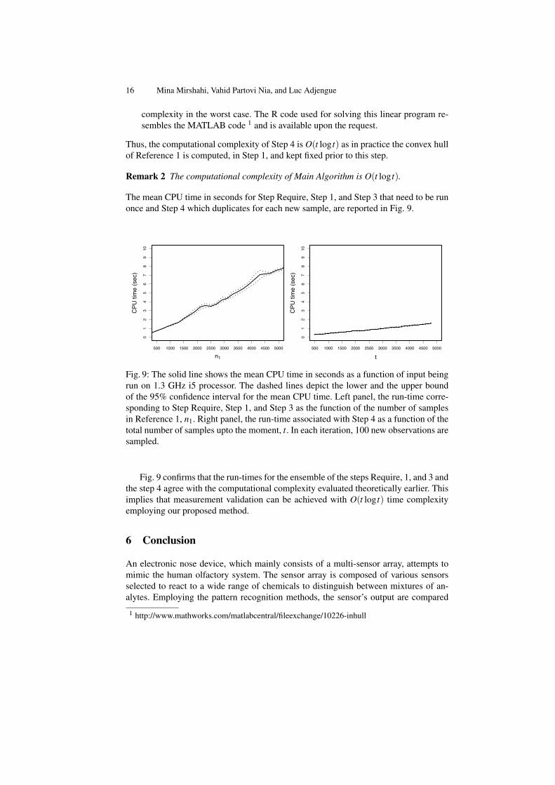
The mean CPU time in seconds for Step Require, Step 1, and Step 3 that need to be runonce and Step 4 which duplicates for each new sample, are reported in Fig. 9.

n1

CPU

tim

e (s

ec)

01

23

45

67

89

10

500 1000 1500 2000 2500 3000 3500 4000 4500 5000

t

CPU

tim

e (s

ec)

01

23

45

67

89

10

500 1000 1500 2000 2500 3000 3500 4000 4500 5000

Fig. 9: The solid line shows the mean CPU time in seconds as a function of input beingrun on 1.3 GHz i5 processor. The dashed lines depict the lower and the upper boundof the 95% confidence interval for the mean CPU time. Left panel, the run-time corre-sponding to Step Require, Step 1, and Step 3 as the function of the number of samplesin Reference 1, n1. Right panel, the run-time associated with Step 4 as a function of thetotal number of samples upto the moment, t. In each iteration, 100 new observations aresampled.

Fig. 9 confirms that the run-times for the ensemble of the steps Require, 1, and 3 andthe step 4 agree with the computational complexity evaluated theoretically earlier. Thisimplies that measurement validation can be achieved with O(t log t) time complexityemploying our proposed method.

6 Conclusion

An electronic nose device, which mainly consists of a multi-sensor array, attempts tomimic the human olfactory system. The sensor array is composed of various sensorsselected to react to a wide range of chemicals to distinguish between mixtures of an-alytes. Employing the pattern recognition methods, the sensor’s output are compared

1 http://www.mathworks.com/matlabcentral/fileexchange/10226-inhull


with reference samples to predict odour concentration. Consequently, the accuracy ofpredicted odour concentration depends heavily on the validity of sensor’s output. Anautomatic procedure that detects the samples’ validity in an online fashion has beena technical shortage and is addressed in this work. A measurement validation processprovides the possibility of attaching a margin of error to the predicted odour concen-trations. Furthermore, it allows taking the subsequent actions such as re-sampling tore-calibrate the models or checking the e-nose device for possible sensor failures. Theproposed measurement validation algorithm initiates a new development in automaticodour detection by minimizing the manpower intervention.

Acknowledgement

The project was funded by the natural sciences and engineering research council ofCanada (NSERC) through the industrial partnership Engage program. Vahid PartoviNia is partially supported by the Canada excellence research chair in data science forreal-time decision making.

Bibliography

Arora, S. and Barak, B. (2009). Computational complexity: A Moden approach. CambridgeUniversity Press.

Artursson, T., Eklov, T., Lundstrom, I., Martensson, P., Sjostrom, M., and Holmberg, M. (2000).Drift correction methods for gas sensors using multivariate methods. Journal of Chemometrics,14:711–723.

Bermak, A., Belhouari, S. B., Shi, M., and Martinez, D. (2006). Pattern recognition techniquesfor odor discrimination in gas sensor array. Encyclopedia of Sensors, X:1–17.

Brys, G., Hubert, M., and Rousseeuw, P. J. (2006). A robustification of independent componentanalysis. Chemometrics, 19:364–375.

Carlo, S. D. and Falasconi, M. (2012). Drift correction methods for gas chemical sensors in artifi-cial olfaction systems: techniques and challenges. Advances in Chemical Sensors, 14:305–326.

Chan, T. M. (1996). Output-sensitive results on convex hulls, extreme points, and related prob-lems. Dicrete and Computational Geometry, 16(4):369–387.

Croux, C. and Haesbroeck, G. (2000). Principal components analysis based on robust estima-tors of the covariance or correlation matrix: Infulence functions and efficiencies. Biometrika,87:603–618.

Dobkin, D. P. and Reiss, S. P. (1980). The complexity of linear programing. Theoritical ComputerScience, 11:1–18.

Donoho, D. L. (1982). Breakdown properties of multivariate location estimators. Ph.D. qualifyingpaper Harvard University.

Du, Q. and Fowler, J. E. (2008). Low-complexity principal component analysis for hyperspec-tral image compression. International Journal of High Performance Computing Applications,22:438–448.

Friedman, J., Hastie, T., and Tibshirani, R. (2008). Sparse inverse covariance estimation with thegraphical lasso. Biostatistics, 9:432–441.

Gardner, J. and Bartlett, P. (1994). A brief history of electronic noses. Sensors and Actuators B:Chemical, 18:211–220.

Golub, G. H. and Loan, C. F. V. (1996). Matrix Computations. The John Hopkins UniversityPress, 3rd edition.

Gupta, A. (2003). Multivariate skew t-distribution. Statistics, 37:359–363.Gutierrez-Osuna, R. (2002). Pattern analysis for machine olfaction: A review. IEEE Sensors

Journal, 2:189–202.Holmes, M. P., Gray, A. G., and Isbell, C. L. (2007). Fast SVD for large-scale matrices. Workshop

on Efficient Machine Learning at NIPS, 58.Hubert, M., Rousseeuw, P. J., and Branden, K. V. (2005). ROBPCA: A new approach to robust

principal component analysis. Thechnometrics, 47:64–79.Hubert, M. and Van der Veeken, S. (2008). Outlier detection for skewed data. Journal of Chemo-

metrics, 22:235–246.Hubert, M. and Vandervieren, E. (2008). An adjusted boxplot for skewed distributions. Compu-

tational Statistics and Data Analysis, 52:5186–5201.Jolliffe, I. (2002). Principal Component Analysis. Springer.Josse, J., Pagès, J., and Husson, F. (2011). Multiple imputation in principal component analysis.

Advances in Data Analysis and Classifications, 5:231–246.Kan, A. R. and Telgen, J. (1981). The complexity of linear programming. Statistica Neerlandica,

2.


Kermiti, M. and Tomic, O. (2003). Independent component analysis applied on gas sensor arraymeasurement data. IEEE Sensors Journal, 3:218–228.

Li, G. and Chen, Z. (1985). Projection-pursuit approach to robust dispersion matrices and prin-cipal components: primary theory and monte carlo. Journal of the American Statistical Asso-ciation, 80:759–766.

McGinley, P. C. and Inc, S. (2002). Standardized odor measurement practices for air qualitytesting. Air and Waste Management Association Symposium on Air Quality MeasurementMethods and Technology, San Francisco, CA.

Mirshahi, M., Partovi Nia, V., and Adjengue, L. (2016). Statistical measurement validation withapplication to electronic nose technology. In Proceedings of the 5th International Conferenceon Pattern Recognition Applications and Methods, pages 407–414.

Ottmann, T., Schuierer, S., and Soundaralakshmi, S. (1995). Enumerating extreme points inhigher dimensions. STACS 95: 12th Annual Symposium on Theoretical Aspects of ComputerScience, Lecture Notes in Computer Science, 900:562–570.

Padilla, M., Perera, A., Montoliu, I., Chaudry, A., Persaud, K., and Marco, S. (2010). Drift com-pensation of gas sensor array data by orthogonal signal correction. Journal of Chemometricsand Intelligent Labrotory System, 100:28–35.

Persaud, K. and Dodd, G. (1982). Analysis of discrimination mechanisms in the mammalianolfactory system using a model nose. Nature, 299:352–355.

Prendergast, L. (2008). A note on sensitivity of principal component subspaces and the effi-cient detection of influential observations in high dimensions. Electronic Journal of Statistics,2:454–467.

Rousseeuw, P. J. and Driessen, K. V. (1999). A fast algorithm for the minumum covariancedeterminant estimator. Technometrics, 41:212–223.

Stahel, W. A. (1981). Robust estimation: Infinitesimal optimality and covariance matrix estima-tors. Ph.D. thesis, ETH, Zurich.

Tibshirani, R. (1996). Regression shrinkage and selection via the lasso. Journal of the RoyalStatistical Society, Series B, 58:267–288.

Zuppa, M., Distante, C., Persaud, K. C., and Siciliano, P. (2007). Recovery of drifting sensorresponses by means of DWT analysis. Journal of Sensors and Actuators, 120:411–416.

an oline data validation algorithm for electronic nose

Documents