an open database for benchmarking guided waves shm

An open database for benchmarking

guided waves SHM algorithms on a

composite full scale outer wing

demonstrator

Alessandro Marzani, Nicola Testoni, Luca De Marchi, Marco Messina,

Ernesto Monaco and Alfonso Apicella

1. Sensors • Position

• Naming conventions

2. Data acquisition

• EMILIA

• Group velocity

• Pitch-catch

3. Data pre-processing

4. Impact testing

• Calibration

• B, S and C-scan

Outline

1. Sensors

Sensors grouping

Sensors position subgroup A1

Sensors position subgroup A2

Sensors position subgroup B

Sensors position subgroup C

Sensors position subgroup D1

Sensors position subgroup D2

Sensors position subgroup E1

Sensors position subgroup E2

Sensors connections group A

Physical cable connection check after SHM showed no faults.

SECTION 0 SECTION 1

0 1 2 3 4 5 6 7 0 1 2 3 4 5 6 7

A1 A2 A3 A4 A5 A6 A7 A8 A11 A12 A13 A14 A15 A16 A17 A18

8 9 10 11 12 13 14 15 8 9 10 11 12 13 14 15

A9 A10 A32 A31 A25 A26 A27 A28 A19 A20 A21 A22 A23 A24 A29 A30

Sensors connections group B

(-) Not used

Physical cable connection check after SHM showed the following faults:

B7: cable connection damaged during test article final assembly

B18: cable damaged during test article final assembly

SECTION 2 SECTION 3

0 1 2 3 4 5 6 7 0 1 2 3 4 5 6 7

B1 B2 B3 B4 B5 B6 B7 B8 B17 B18 B19 B20 B21 B22 B23 B24

8 9 10 11 12 13 14 15 8 9 10 11 12 13 14 15

B9 B10 B11 B12 B13 B14 B15 B16 B25 B26 - - - - - -

Sensors connections group C

(-) Not used


SECTION 4 SECTION 5

0 1 2 3 4 5 6 7 0 1 2 3 4 5 6 7

C1 C2 C3 C4 C5 C6 C7 C8 - - - - - - - -

8 9 10 11 12 13 14 15 8 9 10 11 12 13 14 15

C9 C11 C12 - - - - - - - - - - - - -

Sensors connections group D

(*) Not available due to damaged connector

Physical cable connection check after SHM showed the following faults:

D30: cable connection damaged before test article final assembly

D5: cable connection damaged after impacts

SECTION 6 SECTION 7

0 1 2 3 4 5 6 7 0 1 2 3 4 5 6 7

* D17 D18 D19 D20 D21 D22 D23 D1 D2 D3 D4 D5 D6 D7 D8

8 9 10 11 12 13 14 15 8 9 10 11 12 13 14 15

D24 D25 D26 D27 D28 D29 D30 D31 D9 D10 D11 D12 D13 D14 D15 D16

Sensors connections group E


SECTION 8 SECTION 9

0 1 2 3 4 5 6 7 0 1 2 3 4 5 6 7

E1 E2 E3 E4 E5 E6 E7 E8 E17 E18 E19 E20 E21 E22 E23 E24

8 9 10 11 12 13 14 15 8 9 10 11 12 13 14 15

E9 E10 E11 E12 E13 E14 E15 E16 E25 E26 E26 E28 E29 E30 E31 E32

2. Data acquisition

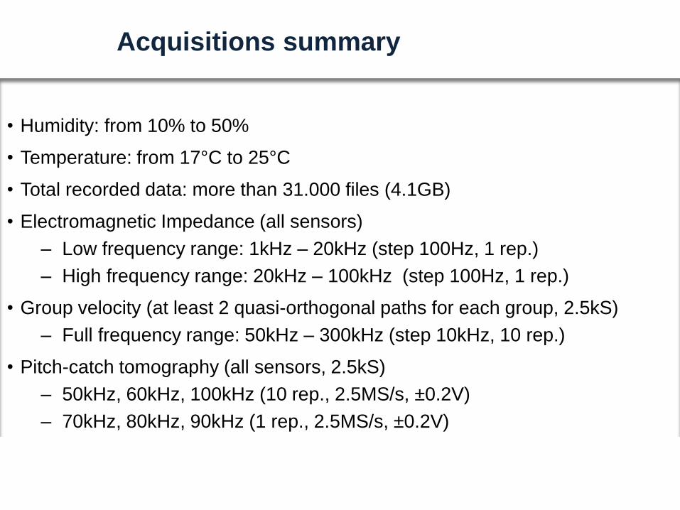
Acquisitions summary

• Humidity: from 10% to 50%

• Temperature: from 17°C to 25°C

• Total recorded data: more than 31.000 files (4.1GB)

• Electromagnetic Impedance (all sensors)

– Low frequency range: 1kHz – 20kHz (step 100Hz, 1 rep.)

– High frequency range: 20kHz – 100kHz (step 100Hz, 1 rep.)

• Group velocity (at least 2 quasi-orthogonal paths for each group, 2.5kS)

– Full frequency range: 50kHz – 300kHz (step 10kHz, 10 rep.)

• Pitch-catch tomography (all sensors, 2.5kS)

– 50kHz, 60kHz, 100kHz (10 rep., 2.5MS/s, ±0.2V)

– 70kHz, 80kHz, 90kHz (1 rep., 2.5MS/s, ±0.2V)

EMI low frequency acquisitions

• Base folder: emiLow

• File name: emiFull_x_y_emi.txt

• File name fields:

x – repetition index (always 00)

y – acquisition index (from 01 to 133)

• Sensors examined section by section: (cfr slides 13-17)

A1-A10, A32, A31, A25-A28, A11-A24, A29, A30, B1-B26, C1-C12, …

• Data file reading routine: readEmiFile.m

dataStruct = readEmiFile('emiLow\emiFull_00_01_emi.txt')

EMI high frequency acquisitions

• Base folder: emiHigh

• File name: emiFullExt_x_y_emi.txt


x – repetition index (always 00)


• Sensors examined section by section: (cfr slides 13-17)

A1-A10, A32, A31, A25-A28, A11-A24, A29, A30, B1-B26, C1-C12, …

• Data file reading routine: readEmiFile.m

dataStruct = readEmiFile('emiHigh\emiFullExt_00_02_emi.txt')

EMI data structure

• dataStruct fields

– warmup: [sec] warmup time for relay configuration

– sec: [num] section index

– src: [num] examined piezo

– sn1: [num] reserved

– sn2: [num] reserved

– f0: [Hz] start frequency

– f1: [Hz] stop frequency

– df: [Hz] frequency increment

– f: [Hz] acquired frequencies

– Z: [Ohm] measured impedance magnitude

– P: [Deg] measured phase angle

Group velocity acquisitions

• Base folder: speed

• File path and name: x\cgFull_x_y_pc.txt


x – repetition index (from 00 to 09)


• Sensors examined frequency by frequency

– 1-10 @ 50kHz, 1-10 @ 60kHz, …

• Data file reading routine: readPcFile.m

dataStruct = readPcFile('speed\00\cgFull_00_03_pc.txt')

Excitation sequence:

1. A22 A12, A20

2. B3 B6, B13

3. B20 B21, B22

4. B20 B23, B24

5. B20 B25, B26

6. C11 C5, C10

7. D11 D6, D15

8. D31 D23, D30

9. E1 E13, E4

10.E32 E24, E31

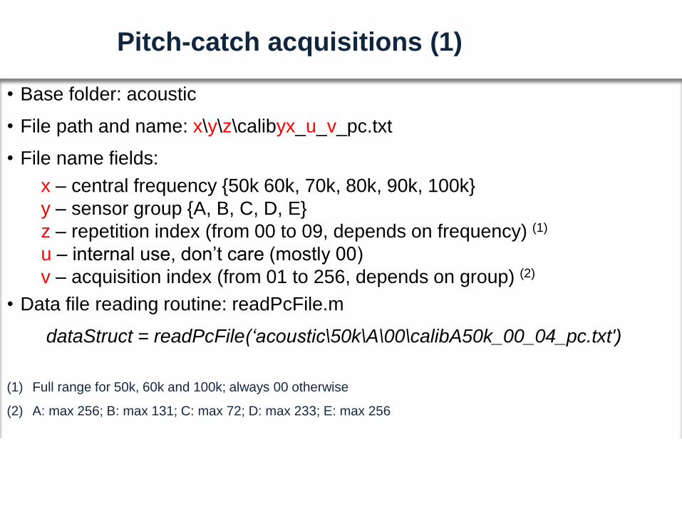
Pitch-catch acquisitions (1)

• Base folder: acoustic

• File path and name: x\y\z\calibyx_u_v_pc.txt


x – central frequency {50k 60k, 70k, 80k, 90k, 100k}

y – sensor group {A, B, C, D, E}

z – repetition index (from 00 to 09, depends on frequency) (1)

u – internal use, don’t care (mostly 00)

v – acquisition index (from 01 to 256, depends on group) (2)

• Data file reading routine: readPcFile.m

dataStruct = readPcFile(‘acoustic\50k\A\00\calibA50k_00_04_pc.txt')

(1) Full range for 50k, 60k and 100k; always 00 otherwise

(2) A: max 256; B: max 131; C: max 72; D: max 233; E: max 256

Pitch-catch acquisitions (2)

• Pitch-catch path pairs acquired section by section: (cfr slides 13-17)

• In case of uneven sequences, the first path is acquired again at the end

1. A1 A2, A3;

2. A1 A4, A5;

3. A1 A6, A7;

4. A1 A8, A9;

5. A1 A10, A32;

6. A1 A31, A25;

7. A1 A26, A27;

8. A1 A28, A2;

9. A2 A1, A3;

10. A2 A4, A5;

11. A2 A6, A7;

12. A2 A8, A9;

13. …

Pitch-catch data structure

• dataStruct fields

– warmup: [sec] warmup time for relay configuration

– sec: [num] section index

– src: [num] actuator piezo

– sn1: [num] receiver piezo 1

– sn2: [num] receiver piezo 2

– wavetype: [string] transmitted waveform type

– fc: [Hz] central frequency

– amp: [V] peat-to-peak voltage

– np: [num] number of periods

– wintype: [string] waveform windowing type

– fs: [Hz] sampling frequency

– Ns: [num] number of acquired samples

– tx: [V] measured transmitted voltage

– rx0: [V] measured received voltage from piezo 1

– rx1: [V] measured received voltage from piezo 2

– t: [s] acquired time instants

3. data pre-processing

Raw recorded data

• Example:

• Sensor B20B23,B24

• EM coupling below 50dB

RX: B23

RX: B24

TX: B20

Pre-processed data

• Exploitation of recorded TX signal

• EM coupling automatic estimation

• EMc reduced below 90dB

• Signal clipping recovery

RX: B23

RX: B24

Clean first arrival

TX: B20

4. Impact testing

6.4 mm thickness

8.3 mm thickness

10 mm thickness

12.5 mm thickness

ramp thickness from 6.4 to 8.3 mm

LWP Thickness distribution

LWP impact energy test

calibration areas

Impact energy calibration

The experimental calibrated energy found

are:

60 J for 6.4 mm thickness;

80 J for 8.3 mm thickness;

120 J for 10 mm thickness.

• Each impact inspected with Olympus

Omniscan C_scan

• Impact gun equipped with an

hemispherical nose 1 inch in

diameter.


B, S and C-scan impact subgroup A2

Impact 1

120J

B, S and C-scan impact subgroup B

Impact 2

80J

B, S and C-scan impact subgroup B

B, S and C-scan impact subgroup C

Impact 1

60J

Impact 2

70J

B, S and C-scan impact subgroup D1

Inasco - 120J impact

B, S and C-scan impact subgroup D2

B, S and C-scan impact subgroup E1

B, S and C-scan impact subgroup E2

an open database for benchmarking guided waves shm

Documents