an optical test of complementarity - univie.ac.at · die emissionseigenschaften des atoms an sich...
TRANSCRIPT
An Optical Test of Complementarity
Thesis
to obtain the doctor’s degree
at the Natural Science Faculty
of the Leopold-Franzens University of Innsbruck
by
Thomas Joseph Herzog
November 2000


To
Rosana and Florian


Summary
The correlated photon pairs created in spontaneous parametric downconversion (PDC)
established in the past a superior source of nonclassical light. The extraordinary correla-
tion properties allowed a large variety of experiments concerning two-photon interference.
Nonlocality in quantum mechanics could be demonstrated among other things. In this
work we discuss some novel interference phenomena.
The basic process is as follows: A pump photon passing through a nonlinear crystal
is reflected back onto itself such that it goes through the crystal twice. During both
passages it has the possibility to create a correlated photon pair. These two emission
processes become indistinguishable if the first photon pair is reflected back onto itself
through the crystal. In contrast to most of the earlier experiments with PDC where
interference shows up in second order correlations (i.e. in a coincidence measurement),
our setup reveals interference already in first order (i.e. in the intensities). However we
will show that we are still dealing with a nonclassical two-photon interference effect. We
present experiments that prove clearly this statement.
In further experiments modify the setup of our experiment in order to investigate
one of the most fundamental principles in quantum mechanics, the principle of comple-
mentarity. It is not possible to devise an arrangement that reveals both particle-like and
wave-like behavior in a single experiment. We will demonstrate this at the example of
interference. If we determine the path of the particle trough the interferometer the inter-
ference pattern will vanish. But if we succeed in erasing this “Welcher-Weg” information
again we will see interference again. We will present experiments that demonstrates this
“Quantum Eraser”. One most important feature of our experiment was that which-path
labeling was accomplished on a system spatially separated from the interfering system.
v

The final experiment was dedicated to a problem that arises from the interpretation of
certain experiments within the realm of cavity-quantum electrodynamics. There exists a
close analogy of our setup to a class of experiments concerning the spontaneous emission
of an atom in the vicinity of a mirror. Usually the experiments are described in terms of
vacuum modes coupling to the atom. We propose a different explanation that depends
on interference between different possibilities of the atom to emit a photon into a certain
mode. We exploit this analogy to discuss several possible tests of both interpretations.
Furthermore we present results of an experimental realization of one of these tests.
vi
Zusammenfassung
Wie sich in den vergangenen Jahren herausgestellt hat stellen die korrelierte Photonen-
paare, wie sie auch bei der spontanen Frequenzkonversion entstehen, eine herausragende
Quelle nichtklassischen Lichtes dar. Ihre außerordentlichen Korrelationseigenschaften
erlaubten eine große Vielfalt an Experimenten uber Zweiphotonen-Interferenz, Nicht-
lokalitat der Quantenmechanik und vieles mehr. In dieser Arbeit berichten wir uber
neue Phanomene zur Zweiphotonen-Interferenz. Folgende Idee liegt dem zugrunde. Ein
Laserstrahl wird durch einen optisch nichtlinearen Kristall geschickt und danach wieder
in sich zuruckreflektiert, so das er ein zweites mal den Kristall passiert. Beide Male
hat er die Moglichkeit ein korreliertes Photonenpaar zu erzeugen. Diese zwei Emis-
sionsprozesse werden ununterscheidbar, wenn das erste Photonenpaar ebenfalls in sich
zuruckreflektiert wird, so das die jeweiligen Moden uberlappen. In den meisten fruheren
Experimenten tritt Interferenz in den Korrelationen zweiter Ordnung (d.h. man mußdie
correlierten Photonen in Koinzidenz detektieren) auf. Hier dagegen zeigt sich Interferenz
bereits in erster Ordnung (d.h. es reicht aus eines der beiden Photonen zu detektieren).
Man kann aber zeigen, daß es sich auch hier um echte Zweiphotonen-Interferenzen han-
delt. Wir stellen Experimente vor, die diese Behauptung belegen.
Wir demonstrieren in weiteren Experimenten, wie unserer Aufbau geandert werden
kann, um eine Untersuchung der Komplementaritat von “Welcher-Weg”-Information
und Interferenz zu ermoglichen. Insbesondere stellen wir eine verbesserte Version eines
“Quantum eraser” vor. Der wichtigste Punkt in diesem Zusammenhang ist, das in
unserem Experiment die Welcher-Weg-Messung an einem System durchgefuhrt wird,
das raumlich getrennt ist von dem interferierendem System.
vii
Das letzte Experiment betrifft ein Problem, daß sich aus der Interpretation gewisser
Experimente ergibt, die auf dem Gebiet der Quantenelektrodynamik in Resonatoren
durchgefuhrt wurden. Es existiert eine enge Analogie zwischen unserem Aufbau und
einer Klasse von Versuchen ber die Anderung der spontane Emission eines Atoms in der
Nahe eines Spiegels. Unser Experiment kann auch als Unterdruckung oder Verstarkung
der Frequenzkonversion in ein gewisses Modenpaar interpretiert werden. Ublicherweise
beschreibt man diese Experimente unter Verwendung des Begriffs des Vakuums, das
an das Atom koppelt und dadurch spontane Emission verursacht. Dieses Vakuum wird
durch die Gegenwart des Spiegels modifiziert, was sich in der Anderung der Lebensdauer
des Atoms und damit der spontanen Emission niedreschlagt.
Wir schlagen eine andere Erklarung vor, die auf der Idee basiert, das Interferenz
auftritt zwischen verschiedenen Moglichkeiten fur das Atom in eine bestimmte Mode
zu emittieren. Die Emissionseigenschaften des Atoms an sich werden nich beeinflusst.
Wir diskutieren verschiedene mogliche experimentelle Tests, die eine Entscheidung zwis-
chen beiden Interpretationen erlauben sollten. Die erwahnte Analogie erlaubt eine Un-
tersuchung derselben Frage am Beispiel der spontanen Frequenzkonversion. Schließlich
prasentieren wir Resultate eines diesbezuglichen Versuchs, der die oben erwahnte Analo-
gie explizit ausnutzt.
viii
Contents
Summary v
Zusammenfassung vii
Table of Contents ix
List of Figures xiii
1 An Overview 1
1.1 Interference . . . . . . . . . . . . . . . . . . . . . . . . . . . . . . . . . . 1
1.2 Complementarity . . . . . . . . . . . . . . . . . . . . . . . . . . . . . . . 3
1.3 A tour through this work . . . . . . . . . . . . . . . . . . . . . . . . . . . 4
2 Spontaneous Parametric Downconversion 6
2.1 Introduction . . . . . . . . . . . . . . . . . . . . . . . . . . . . . . . . . . 6
2.2 General theory . . . . . . . . . . . . . . . . . . . . . . . . . . . . . . . . 8
2.3 The phasematching condition . . . . . . . . . . . . . . . . . . . . . . . . 11
2.4 Our source . . . . . . . . . . . . . . . . . . . . . . . . . . . . . . . . . . . 13
2.5 Two-photon interference . . . . . . . . . . . . . . . . . . . . . . . . . . . 15
3 The “Railcross”-Experiment 18
3.1 Idea . . . . . . . . . . . . . . . . . . . . . . . . . . . . . . . . . . . . . . 18
3.2 Multimode theory . . . . . . . . . . . . . . . . . . . . . . . . . . . . . . . 22
3.3 The experiment . . . . . . . . . . . . . . . . . . . . . . . . . . . . . . . . 25
ix
3.3.1 Basic setup . . . . . . . . . . . . . . . . . . . . . . . . . . . . . . 25
3.3.2 Detection and data acquisition . . . . . . . . . . . . . . . . . . . . 27
3.3.3 Alignment of the experiment . . . . . . . . . . . . . . . . . . . . . 29
3.3.4 Stimulated downconversion . . . . . . . . . . . . . . . . . . . . . 30
3.4 Results and discussion . . . . . . . . . . . . . . . . . . . . . . . . . . . . 33
3.5 Just a classical nonlinear effect? . . . . . . . . . . . . . . . . . . . . . . . 42
3.5.1 Classical model . . . . . . . . . . . . . . . . . . . . . . . . . . . . 42
3.5.2 Anticorrelation at a beamsplitter . . . . . . . . . . . . . . . . . . 46
4 Welcher-Weg Experiments and Quantum Eraser 49
4.1 Introduction . . . . . . . . . . . . . . . . . . . . . . . . . . . . . . . . . . 49
4.2 Welcher-Weg information and loss of interference . . . . . . . . . . . . . 50
4.3 The quantum eraser . . . . . . . . . . . . . . . . . . . . . . . . . . . . . 59
4.4 Requirements on an optimal Welcher-Weg and quantum eraser experiment 62
4.5 Discussion of past experiments . . . . . . . . . . . . . . . . . . . . . . . 63
5 From Theory to Practice – The Two-Photon Quantum Eraser 67
5.1 Introduction . . . . . . . . . . . . . . . . . . . . . . . . . . . . . . . . . . 67
5.2 Experimental setup . . . . . . . . . . . . . . . . . . . . . . . . . . . . . . 68
5.3 Quantum marker and quantum eraser experiments on single photons . . 71
5.3.1 Polarization as quantum marker . . . . . . . . . . . . . . . . . . . 71
5.3.2 Time as quantum marker . . . . . . . . . . . . . . . . . . . . . . . 74
5.3.3 Effect of incomplete which-path information . . . . . . . . . . . . 77
5.4 The two-photon quantum eraser . . . . . . . . . . . . . . . . . . . . . . . 83
5.4.1 Polarization-polarization-scheme . . . . . . . . . . . . . . . . . . . 84
5.4.2 Polarization-time-scheme . . . . . . . . . . . . . . . . . . . . . . . 86
5.5 Possible extension to a delayed choice quantum eraser . . . . . . . . . . . 89
5.6 Conclusion . . . . . . . . . . . . . . . . . . . . . . . . . . . . . . . . . . . 90
6 Can One detect Virtual Photons? 91
6.1 Introduction . . . . . . . . . . . . . . . . . . . . . . . . . . . . . . . . . . 91
x

6.2 A short review of cavity QED . . . . . . . . . . . . . . . . . . . . . . . . 92
6.3 An atom and a mirror - two possible interpretations . . . . . . . . . . . . 94
6.4 Frustrated parametric downconversion . . . . . . . . . . . . . . . . . . . 96
6.5 Two possible tests . . . . . . . . . . . . . . . . . . . . . . . . . . . . . . . 99
6.5.1 A switching experiment to measure the “speed of vacuum” . . . . 99
6.5.2 Looking behind the mirror . . . . . . . . . . . . . . . . . . . . . . 101
6.6 Experimental setup . . . . . . . . . . . . . . . . . . . . . . . . . . . . . . 102
6.7 Results and discussion . . . . . . . . . . . . . . . . . . . . . . . . . . . . 103
7 Conclusions and Outlook 109
Appendix 113
A Properties of LiIO3 113
B The detector 115
C General theory of parametric downconversion 117
D Standard photodetection theory 120
E Multimode treatment of the railcross-experiment 123
F The effect of losses 130
G Calculation of the polarization quantum eraser 133
G.1 Single-count rates . . . . . . . . . . . . . . . . . . . . . . . . . . . . . . . 133
G.2 Coincidence count rate . . . . . . . . . . . . . . . . . . . . . . . . . . . . 137
Acknowledgements 142
References 143
Curriculum Vitae 151
xi

Publications 152
xii

List of Figures
2.1 Sketch of PDC . . . . . . . . . . . . . . . . . . . . . . . . . . . . . . . . 7
2.2 The phasematching condition . . . . . . . . . . . . . . . . . . . . . . . . 12
2.3 Type-I phasematching in L-IO3 . . . . . . . . . . . . . . . . . . . . . . . 13
2.4 Theoretical type-I phasematching in L-IO3 . . . . . . . . . . . . . . . . . 14
2.5 Some experiments on two-photon interference . . . . . . . . . . . . . . . 16
3.1 Setup of the railcross-experiment . . . . . . . . . . . . . . . . . . . . . . 21
3.2 Experiment . . . . . . . . . . . . . . . . . . . . . . . . . . . . . . . . . . 26
3.3 Photograph of the experimental arrangement . . . . . . . . . . . . . . . . 28
3.4 Stimulated PDC to align the experiment . . . . . . . . . . . . . . . . . . 31
3.5 Visibility of stimulated interference . . . . . . . . . . . . . . . . . . . . . 33
3.6 Typical coarse scan to search for interference . . . . . . . . . . . . . . . . 34
3.7 Idler count rate in dependence on the displacement of signal-, idler- and
pump-mirror. . . . . . . . . . . . . . . . . . . . . . . . . . . . . . . . . . 36
3.8 Signal-, idler-, and coincidence count rate upon translating the idler mirror 37
3.9 idler count rate when moving both signal and idler mirror simultaneously 38
3.10 two signal coarse scans with displacement of the idler mirror . . . . . . . 40
3.11 Dependence on the sum of signal- and idler-phase . . . . . . . . . . . . . 41
3.12 Classical model of the experiment . . . . . . . . . . . . . . . . . . . . . . 42
3.13 Visibility according to the classical model . . . . . . . . . . . . . . . . . . 46
3.14 Measurement of the anticorrelation parameter α . . . . . . . . . . . . . . 47
4.1 Einstein’s recoiling slit gedanken experiment . . . . . . . . . . . . . . . . 51
4.2 The gedanken experiment of Wheeler . . . . . . . . . . . . . . . . . . . . 55
xiii
4.3 The microwave cavity which-path detector . . . . . . . . . . . . . . . . . 56
4.4 Quantum erasing in the micromaser setup . . . . . . . . . . . . . . . . . 60
4.5 Experiment of Ou et al. . . . . . . . . . . . . . . . . . . . . . . . . . . . 64
4.6 Experiment of Zou et al. . . . . . . . . . . . . . . . . . . . . . . . . . . . 65
4.7 Quantum eraser of Kwiat et al. . . . . . . . . . . . . . . . . . . . . . . . 66
5.1 The principal setup in all the quantum eraser experiments . . . . . . . . 70
5.2 Quantum marker and quantum eraser using polarization . . . . . . . . . 73
5.3 Time as quantum marker . . . . . . . . . . . . . . . . . . . . . . . . . . . 75
5.4 Quantum marker and quantum eraser using time . . . . . . . . . . . . . 76
5.5 Incomplete quantum eraser in the polarization setup . . . . . . . . . . . 78
5.6 Incomplete which-path information in the polarization setup . . . . . . . 80
5.7 Incomplete which-path information in the time setup . . . . . . . . . . . 81
5.8 First-order interference in the two-photon quantum eraser . . . . . . . . 85
5.9 Two-photon quantum eraser: Polarization-polarization setup . . . . . . . 87
5.10 Two-photon quantum eraser: Polarization-time setup . . . . . . . . . . . 88
5.11 Possible delayed choice quantum eraser . . . . . . . . . . . . . . . . . . . 89
6.1 Radiative decay rate of an atom in presence of a mirror . . . . . . . . . . 93
6.2 An Atom and a mirror–two interpretations . . . . . . . . . . . . . . . . . 96
6.3 The switching experiment . . . . . . . . . . . . . . . . . . . . . . . . . . 100
6.4 Looking behind the mirror . . . . . . . . . . . . . . . . . . . . . . . . . . 102
6.5 Experimental setup . . . . . . . . . . . . . . . . . . . . . . . . . . . . . . 103
6.6 All reflectivities . . . . . . . . . . . . . . . . . . . . . . . . . . . . . . . . 105
6.7 Series of fine scans with lowest reflectivity . . . . . . . . . . . . . . . . . 107
6.8 Series of fine scans with second-lowest reflectivity . . . . . . . . . . . . . 108
B.1 Electronic circuit of passive quenching . . . . . . . . . . . . . . . . . . . 116
F.1 Influence of losses in the railcross-experiment . . . . . . . . . . . . . . . . 130
xiv

“But you see, I can believe a thing without un-derstanding it. It’s all a matter of training”.(Lord Peter Wimsey in “Have his carcase”)
—Dorothy L. Sayers
1 An Overview
1.1 Interference
The double slit experiment “has in it the heart of quantum mechanics. In reality it
contains the only mystery of the theory.” This quotation from Feynman’s “Lectures
on Physics”[Feynman65a] is the best way to express the peculiar role of interference in
physics. Einstein, for instance, was worried above all by the possibility to prepare a
particle in a superposition of different states, a property which is characteristic for a
wave but not for a particle. The state in which the particle will be found cannot be
predicted a priori within quantum mechanics. One can only calculate the probability
to find the particle in a certain state. If it is also not possible to determine the state of
the particle a posteriori (at the detector), then one may observe interference.
In the double-slit setup, for example, the light has two possible ways to go from the
source to the screen corresponding to each one of the slits. From a particle point of view
one would expect naively that each photon should pass exactly through one of both
slits. But that contradicts to the the observation of interference fringes on the screen.
Depending on the path length difference of both paths to the screen the probability to
detect a photon at a certain point shows a strong modulation. But this behavior is the
most important feature of a wave. Loosely speaking one may say that a photon passes
through both slits simultaneously. In such an experiment it is not allowed to attribute
to the photon a definite path.
1

2 1. AN OVERVIEW
It is well known that interference occurs not only with photons but also with material
particles of any kind, for instance with neutrons, electrons and recently also with atoms
and molecules. For these systems interference shows up in a strong modulation of the in-
tensity. However in the last decade another area of research has become well established:
Interferometry with correlated photons as they are created by spontaneous parametric
downconversion. An ultraviolet pump-photon can be converted spontaneously within a
nonlinear crystal with a low probability into two red photons. using these photon pairs
a great variety of experiments to test the foundations of quantum mechanics can be
performed.
Most of the experiments with correlated photons up to the present show interesting
behavior in second-order correlation (coincidence) measurements. Only the two-photon
state as a whole is coherent while each photon on its own does not carry a well defined
phase. Unlike to this we present on this work a novel interference effect that appears
already directly in the photon count rate but which basically relies on the interference
of correlated photons.
Often it is not necessary to use the whole theoretical framework of quantum me-
chanics to understand the results of an interference experiment. One can understand
the main features by applying the well-known Feynman-rules.
1. A quantum system can follow several paths from the source to a measurment de-
vice, from which one cannot infer which path the particle actually choosed (that
means the various paths are indistinguishable). Then one must first add the prob-
ability amplitudes corresponding to each path and take the absolute square from
the result. The result shows interference.
2. The test allows a decision which one of the possibilities has been choosen actually,
the paths are distinguishable. Then the probability of the event is given by the
sum of the probabilities of each alternative. In this case interference is lost.
With these rules it is possible to cover without an extensive need of theory the physics
of all the experiments we discuss in the remainder of the work. For this reason we want
to use them as often as possible throughout this thesis.

1. AN OVERVIEW 3
1.2 Complementarity
Niels Bohr introduced the term “complementarity” to explain the peculiar situation that
there exist mutually incompatible experiments in quantum mechanics. Each experiment
on a quantum object must be described with terms of classical physics because the appa-
ratus that records the outcome is a classical device. On the other hand one has to keep
in mind the inhererent inadequacy of the language of classical physics in the quantum
domain. A classical object has well defined properties (like position and momentum)
independent of a possible observer. However in quantum mechanics it makes only sense
to speak of the properties of the object in context with a particular experiment. Heisen-
berg’s uncertainty relation points out that it is never possible to measure at the same
time both position and momentum of a single quantum object with arbitrary accuracy.
Niels Bohr stated [Schilpp49a, on p.210]:
“Consequently, evidence obtained under different experimental conditions
cannot be comprehended within a single picture, but must be regarded as
complementary in the sense that only the totality of the phenomena exhausts
the possible information about the objects. . . . the study of the complemen-
tary phenomena demands mutually exclusive experimental arrangements”
The most striking example of the complementary behavior of nature is the wave-
particle dualism. A measurement device can yield only information about the wave-or
the particle aspect but it is not possible to observe both aspects simultaneously with
perfect accuracy. For instance let us consider again the double slit situation. Any
attempt to detect which way the particle follows, leads to a degradation of the fringe
pattern on the screen. Perfect determination of the path (by a so-called “Welcher-Weg”
detector) results in a complete disappearance of the interference 1.
Wave-particle complementarity is usually interpreted in terms of Heisenberg’s uncer-
tainty relations. Measuring the path of an interfering particle provokes an uncontrollable1It is noteworthy that it is actually quite difficult to destroy the interference totally. One may place
an 99%-attenuator before one of the slits. In this case one knows with 99% certainty which path theparticle followed. However one can still observe a visibility of about 20% in the interference pattern[Wooters79a]

4 1. AN OVERVIEW
momentum transfer from the path-detector to the particle thereby destroying the co-
herence. However in some circumstances it turns out that no direct interaction between
the interfering particle and the measuring apparatus need be involved. Using correlated
photon pairs one may use one of the photons as the interfering system and the conjugate
photon as label for the different interfering paths. In that case the measurement system
is spatially seperated from the interfering system. Now the correlations between the
interfering system and the measuring system are responsible for the disappearance of
interference.
On the other hand if one does not make use of this which-path information the
following question is obvious: Is it anyhow feasible to erase the distinguishability of the
paths afterwards in such a way that one restores the interference? It turns out that this
is indeed possible. In a carefully designed correlation experiment it is possible to erase
the distinguishability again and to recover interference. This is the idea of the so-called
“quantum eraser”.
1.3 A tour through this work
The central goal of this thesis concerns the problem of interference. We present novel
experiments that demonstrate some of their odd properties. All the experiments de-
scribed here are based on the properties of the correlated photons generated by PDC.
In chapter two we give a general treatment of this nonlinear process. Furthermore we
describe the basic properties of the source used in this work.
Chapter three deals with a new interference effect that forms the basis for all the ex-
periments presented here. It is well known from atomic physics, that external boundary
conditions (for example mirrors) can modify the spontaneous decay of an excited atom.
An analogous experiment is possible with two-photon creation. Using external mirrors,
we were able to either enhance or suppress the emission of the photon pair into a given
mode. The mirrors can be arbitrarily far away from the crystal in contrast to the atom
case. It is characteristic for this experiment that the emission rate depends on the joint
phase of the photon pair. This shows that the phase of the two-photon state cannot be
1. AN OVERVIEW 5
attributed to only one of the two photons. This is a characteristic feature of nonlocality
even if the final outcome of our experiment does not show nonlocal behavior.
The general idea of Welcher-Weg- and quantum-eraser-experiments as a test of com-
plementarity is the topic of chapter four. We discuss the main requirements for an ideal
experiment and analyse in this sense some previous realizations and some proposed ex-
periments. In chapter five we present an improved realization of these ideas, which
relies on the experiment described in chapter three. The peculiarities of our setup allow
a verification of all aspects of Welcher-Weg and quantum eraser experiments discussed
before.
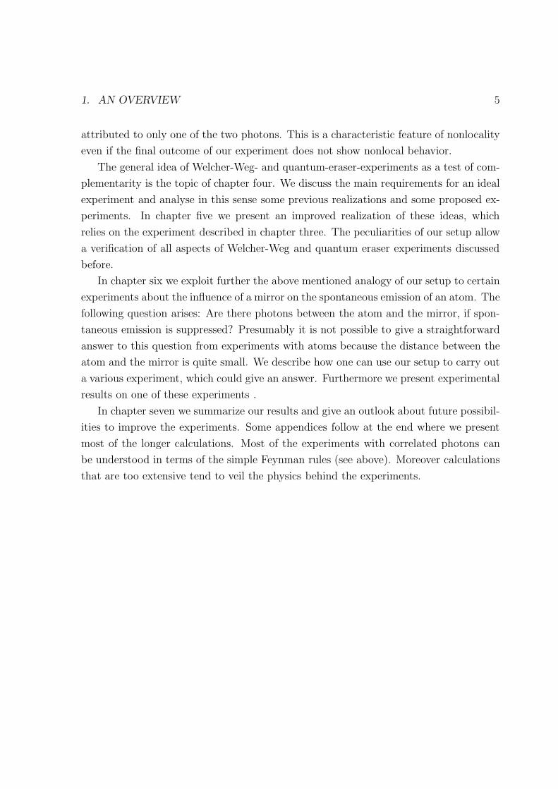
In chapter six we exploit further the above mentioned analogy of our setup to certain
experiments about the influence of a mirror on the spontaneous emission of an atom. The
following question arises: Are there photons between the atom and the mirror, if spon-
taneous emission is suppressed? Presumably it is not possible to give a straightforward
answer to this question from experiments with atoms because the distance between the
atom and the mirror is quite small. We describe how one can use our setup to carry out
a various experiment, which could give an answer. Furthermore we present experimental
results on one of these experiments .
In chapter seven we summarize our results and give an outlook about future possibil-
ities to improve the experiments. Some appendices follow at the end where we present
most of the longer calculations. Most of the experiments with correlated photons can
be understood in terms of the simple Feynman rules (see above). Moreover calculations
that are too extensive tend to veil the physics behind the experiments.
“There was a time when the newspapers said thatonly twelve men understood the theory of relativity.I do not believe there ever was such a time. Theremight have been a time when only one man did, be-cause he was the only guy who caught on, before hewrote his paper. But after people read the paper a lotof people understood the theory of relativity in someway or other, certainly more than twelve. On theother hand I think I can safely say that nobody un-derstands quantum mechanics.”
Richard P. Feynman 1965
2 Spontaneous Parametric
Downconversion
2.1 Introduction
It is necessary to understand the main features of spontaneous parametric downcon-
version, because this process forms the basis for all the experiments described in the
following sections.
This long expression stands for a quite simple phenomenon: Due to an interaction
in a nonlinear crystal, a pump photon can convert with a small probability (≈ 10−6)
spontaneously into two photons with lower energy, historically called the “signal” and
“idler”. These photons possess very strong correlation properties [Burnham70a]: They
are created almost simultaneously within a time window that is given by the inverse of
the emitted bandwidth (≈ 100fs [Hong87a]). Furthermore the frequencies are highly
correlated (within the linewidth of the pump) because of energy conservation. So far
6

2. SPONTANEOUS PARAMETRIC DOWNCONVERSION 7
the situation is quite similar to the two-photon decay of free atoms as it was used for
instance in [Aspect82a]. Unfortunately the atomic two photon source suffers from an
unsatisfactory angular correlation because it concerns a three-particle process (atom
and two photons). In this respect PDC is superior, because, due to the large mass of
the crystal, the propagation directions of the correlated photons are strongly correlated
as well. That means, if we measure a photon in a given direction, we can predict the
direction of the correlated photon with high accuracy (a few millirad depending on the
size of the interaction volume).
1
1'
2
2'3
3'
Figure 2.1: The principle of spontaneous PDC: A pump photon can be converted withlow probability into two photons with lower frequency. The modes on opposite sides ofthe pump beam are correlated to each other. Three pairs of such correlated modes areshown (correlated modes are indicated by the same linestyle).
The conservation laws do not severely restrict the directions of the emitted photons.
A broad range of directions is possible. The frequencies of the pairs can be degenerate
(equal) or non-degenerate (unequal). Photons of one specific color are emitted on a cone
around the pump beam axis. The opening angle of this cone depends on the wavelength
of the photon. Fig. 2.1 depicts the situation for three such modes selected out by irises.
In a simplified manner the emitted state can be written as:
|Ψ〉 = 1√3
(|ks1
〉1|ki1〉2 + |ks2〉1|ki2〉2 + |ks3
〉1|ki3〉2 · · ·)
(2.1)
This state is a canonical example of an entangled state which can be used to demon-
strate nonlocality in quantum mechanics [Horne89a].
8 2. SPONTANEOUS PARAMETRIC DOWNCONVERSION
2.2 General theory
We now turn to a more complete description of PDC that takes into account the finite co-
herence length of the emitted light. The nature of the phenomenon is similar to the spon-
taneous emission of atoms inherently an quantum mechanical effect. It is not possible to
explain consistently all the properties by a classical field theory. The generated signal-
and idler fields must be quantized fully whereas the pump field can be assumed to be in
a classical coherent state because of its high intensity: Ep =∫dωpap(ωp)e
ikpr−iω(kpt)+c.c.
If the nonlinear interaction is weak enough, we can use first order perturbation theory
(we neglect small effects like upconversion of the photons back into the pump or creation
of more than one photon pair at the same time). Going through this calculation yields
for the resulting state (for details see appendix B):
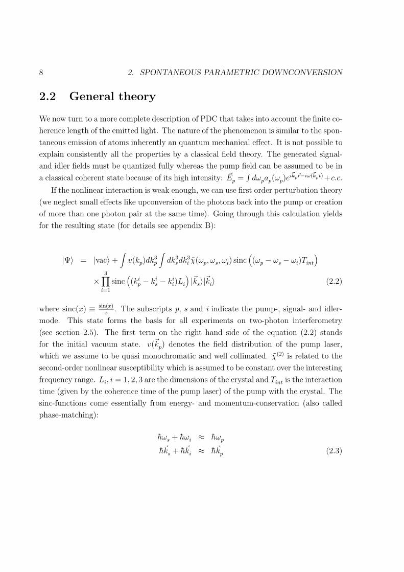
|Ψ〉 = |vac〉+∫
v(kp)dk3p
∫dk3
sdk3i χ(ωp, ωs, ωi) sinc
((ωp − ωs − ωi)Tint
)
×3∏
i=1
sinc((kip − kis − kii)Li
)|ks〉|ki〉 (2.2)
where sinc(x) ≡ sin(x)x
. The subscripts p, s and i indicate the pump-, signal- and idler-
mode. This state forms the basis for all experiments on two-photon interferometry
(see section 2.5). The first term on the right hand side of the equation (2.2) stands
for the initial vacuum state. v(kp) denotes the field distribution of the pump laser,
which we assume to be quasi monochromatic and well collimated. χ(2) is related to the
second-order nonlinear susceptibility which is assumed to be constant over the interesting
frequency range. Li, i = 1, 2, 3 are the dimensions of the crystal and Tint is the interaction
time (given by the coherence time of the pump laser) of the pump with the crystal. The
sinc-functions come essentially from energy- and momentum-conservation (also called
phase-matching):
hωs + hωi ≈ hωp
hks + hki ≈ hkp (2.3)
2. SPONTANEOUS PARAMETRIC DOWNCONVERSION 9
The phase-matching condition confines the range of directions into which photons of
a certain color are emitted. We will elaborate on this more in the next section. We have
assumed that the interaction time and the dimensions of the crystal are large compared
with the oscillation period and the wavelength of the light fields. Therefore we can
replace the sinc-functions by delta-functions and energy and momentum conservation
are exact fulfilled.
In reality we can assume energy conservation as exact because of the long coherence
length of the pump laser in our experiments. However for phasematching this is not
necessarily the case. It is not only the size of the crystal that limits the phasematching
in the transverse direction but also the diameter and the divergency of the pump beam
(typically about one mrad).
For the present discussion we assume the pump-, signal- and idler-field each as plane
waves with exactly defined spatial modes given by the phase-matching condition. Then
we can simplify Eq. (2.2):
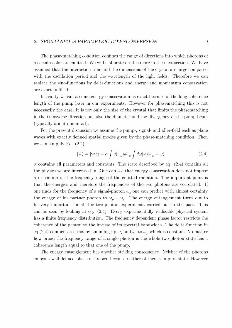
|Ψ〉 = |vac〉+ α∫
v(ωp)dωp
∫dω|ω〉|ωp − ω〉 (2.4)
α contains all parameters and constants. The state described by eq. (2.4) contains all
the physics we are interested in. One can see that energy conservation does not impose
a restriction on the frequency range of the emitted radiation. The important point is
that the energies and therefore the frequencies of the two photons are correlated. If
one finds for the frequency of a signal-photon ωs one can predict with almost certainty
the energy of his partner photon to ωp − ωs. The energy entanglement turns out to
be very important for all the two-photon experiments carried out in the past. This
can be seen by looking at eq. (2.4). Every experimentally realizable physical system
has a finite frequency distribution. The frequency dependent phase factor restricts the
coherence of the photon to the inverse of its spectral bandwidth. The delta-function in
eq.(2.4) compensates this by summing up ωs and ωi to ωp which is constant. No matter
how broad the frequency range of a single photon is the whole two-photon state has a
coherence length equal to that one of the pump.
The energy entanglement has another striking consequence. Neither of the photons
enjoys a well defined phase of its own because neither of them is a pure state. However

10 2. SPONTANEOUS PARAMETRIC DOWNCONVERSION
the entire two-photon state as a whole has a defined phase. Moreover the photon pair
also carries the information about the phase of the pump. This behavior has been
verified experimentally [Ou90a].
The frequency entanglement is also responsible for the tight time correlation of the
photon pairs. This can be seen by the following consideration. We have to calculate the
probability to see a signal-photon at time ts and the correlated idler-photon at time ti.
The standard photodetection theory [Glauber63a] gives:
G2(ts, ti) = 〈Ψ|E−s (ts)E−i (ti)E+i (ti)E
+s (ts)|Ψ〉
= |E+i (ti)E
+s (ts)|Ψ〉|2 (2.5)
E(s,i+)ts,i and E
(s,i−)ts,i are the positive and negative frequency part of the electric
fields for the signal (idler) mode which are related by:(E
(−)s,i (ts,i)
)†= E
(+)s,i (ts,i) =
∫dωs,ie
iωs,its,iηs,i(ωs,i)as,i(ωs,i) (2.6)
Here we have assumed interference filters in front of the detectors described by the
functions ηsωs and ηiωi. Furthermore we assume a monochromatic pump such that we
can rewrite eq. (2.4) to : |Ψ〉 = ∫dω|ω〉|ωP −ω〉. By putting this into eq.(2.5) and after
a little bit of algebra we arrive at the following expression:
G2(ts, ti) =∣∣∣∣∫
dωηsωη iωP − ωeiω(ti−ts)∣∣∣∣2 (2.7)
This clearly vanishes if the time difference is larger than the inverse of the bandwidth
∆ω of the interference filters. Because of the large possible frequency range there results
a tight time correlation of the two photons. The lower limit of this correlation must be
understood as due to the energy-time uncertainty relation. The birth moment of the
photons cannot be better defined than ∆t ≈ h∆ω
. The effective bandwidth ∆ω of the
detected photons is in practice restricted by filters in front of the detectors. It is also
possible that irises in front of the detectors limit the bandwidth further because the
color of the photon depends on its emission direction. Restricting the acceptance angle
of the detector limits also the frequency range seen by the detector. This behavior has
been verified in several experiments [Hong87a, Kwiat92b, Steinberg92b].
2. SPONTANEOUS PARAMETRIC DOWNCONVERSION 11
2.3 The phasematching condition
Phasematching (or momentum conservation) together with energy conservation defines
the directions into which the correlated photons can be emitted. One may view the
physical meaning of the phasematching condition as constructive interference between
the light fields created within the crystal at every point along the pump beam. These
conditions must be fulfilled within the crystal. Due to the dispersion of the refractive
index within the crystal this imposes some constraints. In fact it is only possible in
birefringent crystals possible to match both conditions. These materials are character-
ized by an ordinary refractive index no vertical to the optical axis and an extraordi-
nary one ne parallel the axis. There exist two possible phasematching configuretaions
[Dimitriev91a, Yariv89a]:
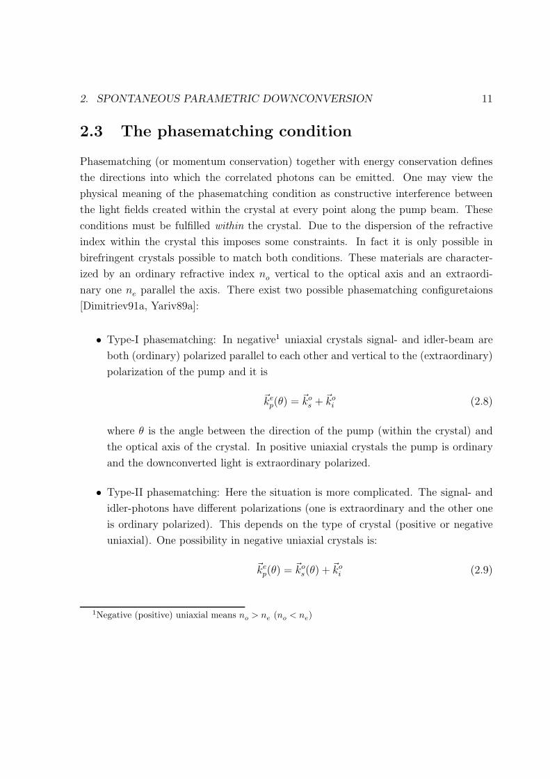
• Type-I phasematching: In negative1 uniaxial crystals signal- and idler-beam are
both (ordinary) polarized parallel to each other and vertical to the (extraordinary)
polarization of the pump and it is
kep(θ) =kos +
koi (2.8)
where θ is the angle between the direction of the pump (within the crystal) and
the optical axis of the crystal. In positive uniaxial crystals the pump is ordinary
and the downconverted light is extraordinary polarized.
• Type-II phasematching: Here the situation is more complicated. The signal- and
idler-photons have different polarizations (one is extraordinary and the other one
is ordinary polarized). This depends on the type of crystal (positive or negative
uniaxial). One possibility in negative uniaxial crystals is:
kep(θ) =kos(θ) +
koi (2.9)
1Negative (positive) uniaxial means no > ne (no < ne)

12 2. SPONTANEOUS PARAMETRIC DOWNCONVERSION
Figure 2.2: Geometry of noncollinear type-I phasematching in negative uniaxial crystals.
In our experiments we used noncollinear nondegenerate type-I phasematching in
LiIO3. Therefore we have to go into some detail on this issue. Following the geometry
of Fig. (2.2) we start from eq.(2.8). Taking the absolute square we arrive at:
koi2 = kep
2(θ) + kos2 − 2kes(θ)k
os cos(φs)
Resolving for cos(φs) and substituting the usual relation |kj| = nj2πλj
(j = p, s, i) we get
finally:
cos(φs) =1
2ωsωpnsnp(θ)
ω2sn
2s + ω2
pnp(θ)2 − ω2
i n2i
(2.10)
θ is the angle between the pump and the optical axis. We can now calculate (using
energy conservation hωp = hωs + hωi) the color of the photon depending on the angle
to the pump beam. By applying Snell’s law one can transform the internal angles back
to the external angles.
2. SPONTANEOUS PARAMETRIC DOWNCONVERSION 13
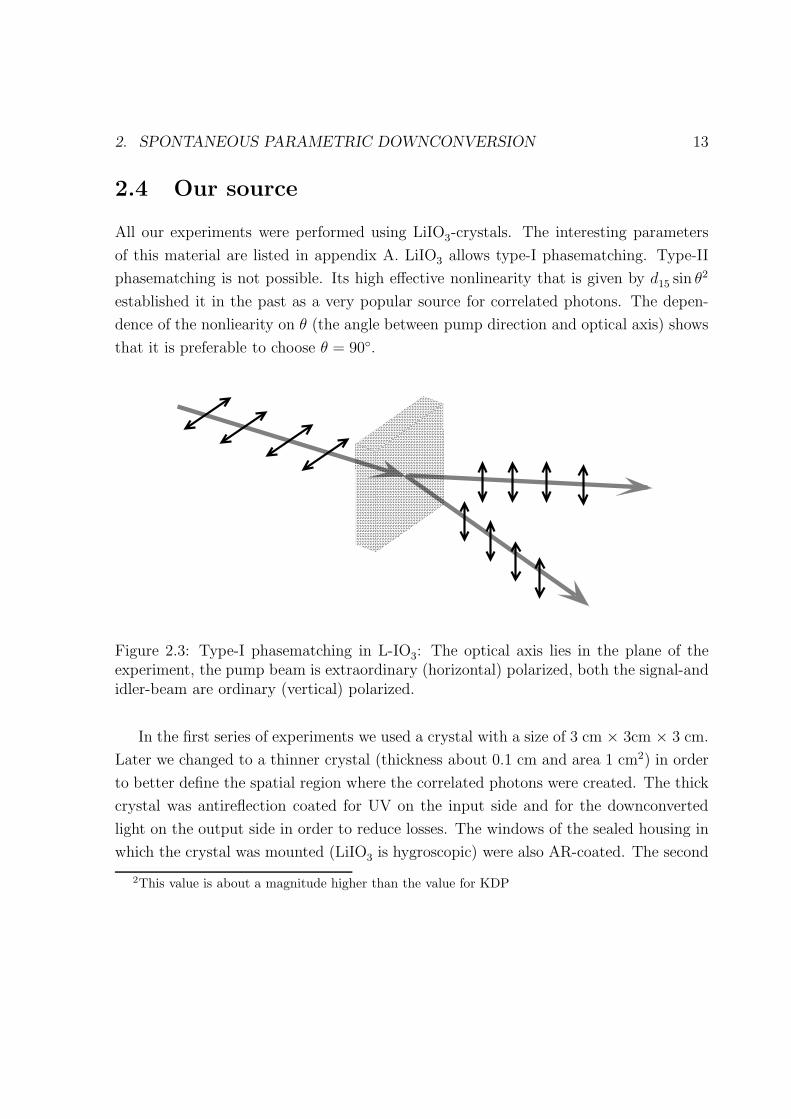
2.4 Our source
All our experiments were performed using LiIO3-crystals. The interesting parameters
of this material are listed in appendix A. LiIO3 allows type-I phasematching. Type-II
phasematching is not possible. Its high effective nonlinearity that is given by d15 sin θ2
established it in the past as a very popular source for correlated photons. The depen-
dence of the nonliearity on θ (the angle between pump direction and optical axis) shows
that it is preferable to choose θ = 90.
Figure 2.3: Type-I phasematching in L-IO3: The optical axis lies in the plane of theexperiment, the pump beam is extraordinary (horizontal) polarized, both the signal-andidler-beam are ordinary (vertical) polarized.
In the first series of experiments we used a crystal with a size of 3 cm × 3cm × 3 cm.
Later we changed to a thinner crystal (thickness about 0.1 cm and area 1 cm2) in order
to better define the spatial region where the correlated photons were created. The thick
crystal was antireflection coated for UV on the input side and for the downconverted
light on the output side in order to reduce losses. The windows of the sealed housing in
which the crystal was mounted (LiIO3 is hygroscopic) were also AR-coated. The second
2This value is about a magnitude higher than the value for KDP

14 2. SPONTANEOUS PARAMETRIC DOWNCONVERSION
Figure 2.4: Calculation of the direction in which the downconverted light is emittedversus the wavelength. The different curves are labeled by the angle between pump andoptical axis.
crystal was not coated at all. We could only reduce the losses a little bit by removing
the windows from the container and heating the crystal to avoid a buildup of moisture.
Our pump source was a large frame INNOVA400 Ar+ion laser from Coherent with
single frequency and single mode capability. We operated the laser in the UV-regime at
351.1 nm. The maximum power was about 0.8 W (single frequency). In order to achieve
a pure single spatial mode we had to attenuate the laser further to typically 100-300
mW. The originally vertical polarization was changed to horizontal by beam steering
mirrors. The beam divergency of the beam was about 0.3 mrad. We placed a weak
focussing lens (focal length 2m) in front of the crystal. This was a compromise between
a better definition of the mode volume within the crystal and a larger divergency of the
2. SPONTANEOUS PARAMETRIC DOWNCONVERSION 15
beam.
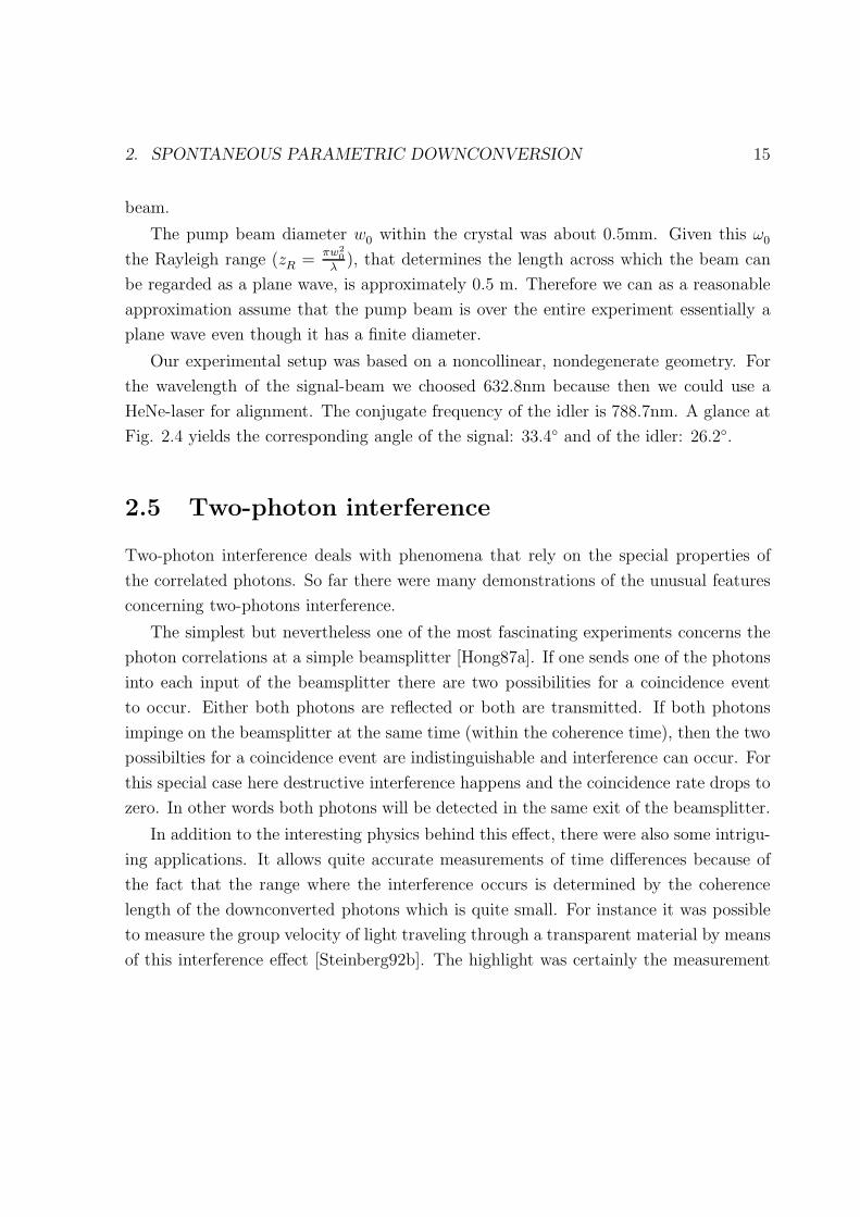
The pump beam diameter w0 within the crystal was about 0.5mm. Given this ω0
the Rayleigh range (zR =πw2
0
λ), that determines the length across which the beam can
be regarded as a plane wave, is approximately 0.5 m. Therefore we can as a reasonable
approximation assume that the pump beam is over the entire experiment essentially a
plane wave even though it has a finite diameter.
Our experimental setup was based on a noncollinear, nondegenerate geometry. For
the wavelength of the signal-beam we choosed 632.8nm because then we could use a
HeNe-laser for alignment. The conjugate frequency of the idler is 788.7nm. A glance at
Fig. 2.4 yields the corresponding angle of the signal: 33.4 and of the idler: 26.2.
2.5 Two-photon interference
Two-photon interference deals with phenomena that rely on the special properties of
the correlated photons. So far there were many demonstrations of the unusual features
concerning two-photons interference.
The simplest but nevertheless one of the most fascinating experiments concerns the
photon correlations at a simple beamsplitter [Hong87a]. If one sends one of the photons
into each input of the beamsplitter there are two possibilities for a coincidence event
to occur. Either both photons are reflected or both are transmitted. If both photons
impinge on the beamsplitter at the same time (within the coherence time), then the two
possibilties for a coincidence event are indistinguishable and interference can occur. For
this special case here destructive interference happens and the coincidence rate drops to
zero. In other words both photons will be detected in the same exit of the beamsplitter.
In addition to the interesting physics behind this effect, there were also some intrigu-
ing applications. It allows quite accurate measurements of time differences because of
the fact that the range where the interference occurs is determined by the coherence
length of the downconverted photons which is quite small. For instance it was possible
to measure the group velocity of light traveling through a transparent material by means
of this interference effect [Steinberg92b]. The highlight was certainly the measurement
16 2. SPONTANEOUS PARAMETRIC DOWNCONVERSION
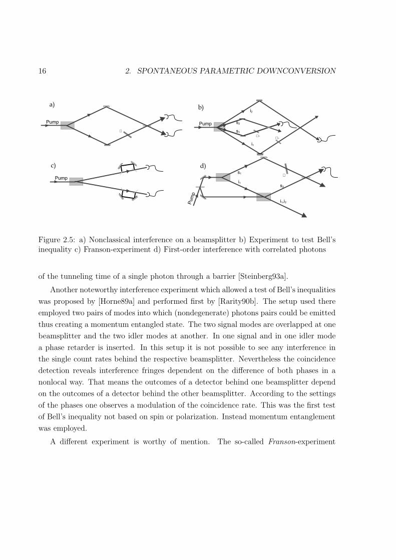
Figure 2.5: a) Nonclassical interference on a beamsplitter b) Experiment to test Bell’sinequality c) Franson-experiment d) First-order interference with correlated photons
of the tunneling time of a single photon through a barrier [Steinberg93a].
Another noteworthy interference experiment which allowed a test of Bell’s inequalities
was proposed by [Horne89a] and performed first by [Rarity90b]. The setup used there
employed two pairs of modes into which (nondegenerate) photons pairs could be emitted
thus creating a momentum entangled state. The two signal modes are overlapped at one
beamsplitter and the two idler modes at another. In one signal and in one idler mode
a phase retarder is inserted. In this setup it is not possible to see any interference in
the single count rates behind the respective beamsplitter. Nevertheless the coincidence
detection reveals interference fringes dependent on the difference of both phases in a
nonlocal way. That means the outcomes of a detector behind one beamsplitter depend
on the outcomes of a detector behind the other beamsplitter. According to the settings
of the phases one observes a modulation of the coincidence rate. This was the first test
of Bell’s inequality not based on spin or polarization. Instead momentum entanglement
was employed.
A different experiment is worthy of mention. The so-called Franson-experiment

2. SPONTANEOUS PARAMETRIC DOWNCONVERSION 17
[Franson89a] relies on the energy-time entanglement of the correlated photons. It
resembles the original Einstein-Podolsky-Rosen-paradox [Einstein35a] because conti-
nous variables are used. The signal- and idler photons are sent into seperate Mach-
Zehnder interferometer. Each Interferometer has path lengths which differ by more
than a coherence length, such it is not possible to see interference in the singles count
rates. However, if the difference of the path length differences is equal (again within
the photon’s coherence time), high-visibility fringes can be observed in coincidence
[Kwiat90a, Ou90b, Brendel91a, Brendel92a, Kwiat93a].
Most of the experiments performed up to now have dealed with second-order inter-
ference. Recently a new class of two-photon experiments was discovered showing the
interesting features already in first order [Zou91a]. In these experiments two crystals are
used both pumped by the same laser. The two signal-modes from each crystal are over-
lapped on a beamsplitter. No interference can be seen because one can distinguish the
origin of the photons by detecting the idler in coincidence. According to the Feynman-
rules no interference can be observed. On the other hand one can overlap the two idler
beams completely by sending one idler through the other crystal. Then it is no longer
possible to distinguish the two signal-beams and first-order fringes are visible.
Some possible applications should still be mentioned. First of all it has been pro-
posed [Mandel84a] to use the strong correlation properties for communication free of
background. By imprinting the same information on both the signal- and idler-beam,
the receiver is able, even in the case of a poor signal, to decipher a message by means of
a coincidence measurement. Quantum cryptography is another subject concerning the
security and confidence of information channels[Bennett92b]. Several proposals have
been made relying on the quantum nature of light. Among others it has been suggested
to use the nonlocal correlation arising from entangled states [Ekert91a]. Every attempt
of an eavesdropper will be disclosed afterwards by tests of Bell’s inequality which cannot
be violated in presence of the eavesdropper. There are also a rich variety of other exper-
iments using correlated photons. A lot of experiments are still waiting for a realization,
for instance quantum teleportation [Bennett93a]. This short review should only give an
idea of the rich physics which is inherent in correlated photons.
“The scenery in the play was beautiful, but theactors got in front of it.”’
Alexander Woollcott
3 The “Railcross”-Experiment
3.1 Idea
Most experiments on two-photon interference, published up to now, are based on mea-
surements in coincidence and exhibit so-called second-order interference (one exception
was the experiment described in [Zou91a]). In this chapter we report on a new setup
revealing its two-photon behavior already in first order [Herzog94a].
The experiment described here connects the non-classical behaviour of PDC-photons
with the field of cavity-quantum-electrodynamics in the sense that it demonstrates how
the creation of a two-photon field can be manipulated by changing external boundary
conditions. Placing an atom in front of a mirror [Drexhage74a] results in modification
of the spontaneous emission rate depending on the position of the mirror. The photon
can reach the detector either directly or via the mirror. Indistinguishability of these
paths leads to interference and thereby to suppression or enhancement of spontaneous
emission. Our experiment was quite analogous in the sense that we also manipulated
the boundary conditions, thereby changing the emission of the photon pairs into certain
modes. We prepared a situation with two indistinguishable possibilities to create a
photon pair. According to Feynman (chapter 1) this leads to interference. The analogy
with the atom-mirror case and its implications are the main subject of chapter 6 and we
go into more detail about this topic there.
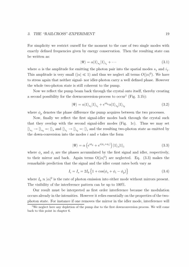
Let us consider the process of PDC. By this we mean, as explained in the last chapter,
the splitting of a pump photon into two photons with lower frequency (see Fig. 3.1a).
18
3. THE “RAILCROSS”-EXPERIMENT 19
For simplicity we restrict ourself for the moment to the case of two single modes with
exactly defined frequencies given by energy conservation. Then the resulting state can
be written as:
|Ψ〉 = α|1〉s1|1〉i1 + · · · (3.1)
where α is the amplitude for emitting the photon pair into the spatial modes s1 and i1.
This amplitude is very small (|α| 1) and thus we neglect all terms O(|α|2). We have
to stress again that neither signal- nor idler-photon carry a well defined phase. However
the whole two-photon state is still coherent to the pump.
Now we reflect the pump beam back through the crystal onto itself, thereby creating
a second possibility for the downconversion-process to occur1 (Fig. 3.1b):
|Ψ〉 = α|1〉s1|1〉i1 + eiφpα|1〉s2
|1〉i2 (3.2)
where φp denotes the phase difference the pump acquires between the two processes.
Now, finally we reflect the first signal-idler modes back through the crystal such
that they overlap with the second signal-idler modes (Fig. 1c). Thus we may set
|〉s1→ |〉s2
=: |〉s and |〉i1 → |〉i2 =: |〉i and the resulting two-photon state as emitted by
the down-conversion into the modes i and s takes the form
|Ψ〉 = α(eiφp + ei(φs+φi)
)|1〉s|1〉i (3.3)
where φs and φi are the phases accumulated by the first signal and idler, respectively,
to their mirror and back. Again terms O(|α|2) are neglected. Eq. (3.3) makes the
remarkable prediction that the signal and the idler count rates both vary as
Ii = Is = 2I0
1 + cos(φs + φi − φp)
(3.4)
where I0 ∝ |α|2 is the rate of photon emission into either mode without mirrors present.
The visibility of the interference pattern can be up to 100%.
Our result must be interpreted as first order interference because the modulation
occurs already in the intensities. However it relies essentially on the properties of the two-
photon state. For instance if one removes the mirror in the idler mode, interference will1We neglect here any depletion of the pump due to the first downconversion process. We will come
back to this point in chapter 6.

20 3. THE “RAILCROSS”-EXPERIMENT
b)
c)
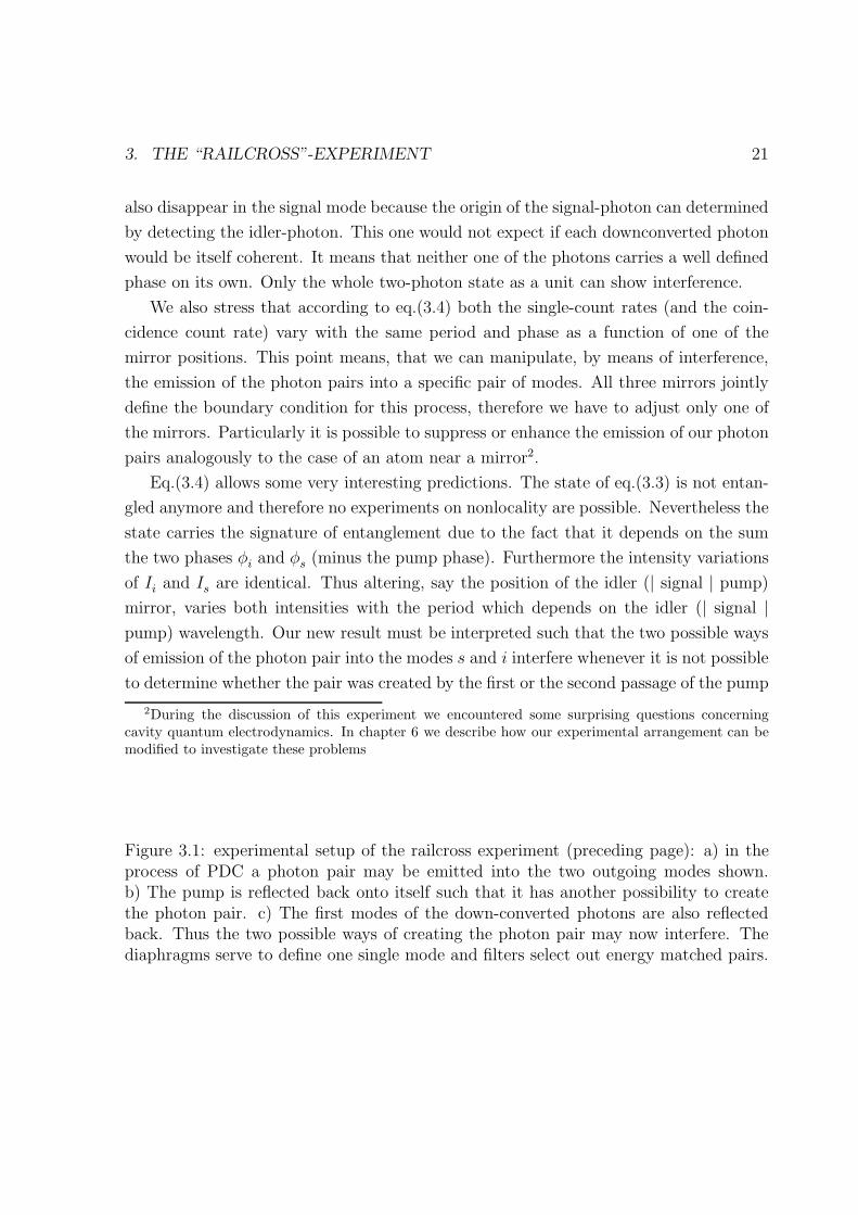
3. THE “RAILCROSS”-EXPERIMENT 21
also disappear in the signal mode because the origin of the signal-photon can determined
by detecting the idler-photon. This one would not expect if each downconverted photon
would be itself coherent. It means that neither one of the photons carries a well defined
phase on its own. Only the whole two-photon state as a unit can show interference.
We also stress that according to eq.(3.4) both the single-count rates (and the coin-
cidence count rate) vary with the same period and phase as a function of one of the
mirror positions. This point means, that we can manipulate, by means of interference,
the emission of the photon pairs into a specific pair of modes. All three mirrors jointly
define the boundary condition for this process, therefore we have to adjust only one of
the mirrors. Particularly it is possible to suppress or enhance the emission of our photon
pairs analogously to the case of an atom near a mirror2.
Eq.(3.4) allows some very interesting predictions. The state of eq.(3.3) is not entan-
gled anymore and therefore no experiments on nonlocality are possible. Nevertheless the
state carries the signature of entanglement due to the fact that it depends on the sum
the two phases φi and φs (minus the pump phase). Furthermore the intensity variations
of Ii and Is are identical. Thus altering, say the position of the idler (| signal | pump)
mirror, varies both intensities with the period which depends on the idler (| signal |pump) wavelength. Our new result must be interpreted such that the two possible ways
of emission of the photon pair into the modes s and i interfere whenever it is not possible
to determine whether the pair was created by the first or the second passage of the pump
2During the discussion of this experiment we encountered some surprising questions concerningcavity quantum electrodynamics. In chapter 6 we describe how our experimental arrangement can bemodified to investigate these problems
Figure 3.1: experimental setup of the railcross experiment (preceding page): a) in theprocess of PDC a photon pair may be emitted into the two outgoing modes shown.b) The pump is reflected back onto itself such that it has another possibility to createthe photon pair. c) The first modes of the down-converted photons are also reflectedback. Thus the two possible ways of creating the photon pair may now interfere. Thediaphragms serve to define one single mode and filters select out energy matched pairs.

22 3. THE “RAILCROSS”-EXPERIMENT
through the downconversion crystal.
We want to mention that the phenomenon can be interpreted slightly differently
[Milonni95b]. This description rests on the interpretation, that PDC can be seen as
stimulated by the vacuum fluctuations (see also e.g. [Yariv89a]). In the first of these
processes the incoming pump mixes with the incoming vacuum idler field to generate a
signal photon which then propagates via the signal mirror to its detector. The amplitude
of this process is A1 = Aeiφs . In the second process a signal photon may be created by
mixing the reflected pump with the reflected idler vacuum field. The corresponding
amplitude includes the pump and idler phase but not the signal phase: A2 = Aei(φp−φi).
Thus the probability to count the a signal photon is again:
|A1 + A2|2 = |A|2|eiφs + ei(φp−φi)|2 ∝ 1 + cos(φs + φi − φp) (3.5)
As one expects, the final result remains the same3.
3.2 Multimode theory
A more realistic description of the two-photon generation has to take into account the
finite frequency bandwidth of the emitted light. We still assume that the pump and
the downconverted photons are represented by plane waves. The spectral frequency
distribution of pump-light is described by v(ωp), the distributions ηs(ωs) and ηi(ωi) of
the signal and the idler light are determined by the interference filters in front of the
detectors.
Then we can use the theory of PDC developed in Chapter 2.2. Here omit the detailed
calculation which is given in Appendix E. We assume again perfect phase matching.
Using standard photodetection theory (Appendix D) we arrive et the following expression
for the signal-singles count rate (the idler count rate cn be obtained in an analogous way):
3In the same reference [Milloni95b] a detailed description within the framework of quantum electro-dynamics is given. The result was that the interpretation of the experiment as a new cavity QED effectis valid in spite of the puzzling features inherent to the phenomenon (see also chapter 6).
3. THE “RAILCROSS”-EXPERIMENT 23
RS = 2|α|2∫
dωp|v(ωp)|2∫
dωη2s(ω)
+∫
dωp|v(ωp)|2eiωp(τav−τp)∫
dωη2s(ω)e
iω(τs−τi) cos(Φs0 + Φi0 − Φp0)
⇓
RS = 2|α|2Ipηs1 + VpV cos(Φs0 + Φi0 − Φp0)
(3.6)
with
Ip =∫
dωp|v(ωp)|2
ηs =∫
dωη2s(ω)
Vp =1
Ip
∫dωp|v(ωp)|2eiωp(τav−τp) (3.7)
VS =1
ηs
∫dωη2
s(ω)eiω(τs−τi) (3.8)
τp, τs, τi are the traveling times of the pump-, signal- and idler-beam resp. from the
crystal to the coresponding mirror and back. τav := τs+τi2
is a measure of the average
distance from the crystal to the signal- and idler mirror. Φk = ωkτk, k ∈ p0, s0, i0denote the phase settings of the different mirrors. Ip is the intensity of the pump, v(ωp)
and ηs(ωs) are the frequency spectrum of the pump and of the interference filter in
front of the signal-detector respectively. The finite efficiency of the detector itself can
be included in this function. The contrast of the interference pattern is governed by the
visibility functions V and Vp. They are given by the fourier-transform of the frequency
distributions of the signal-photons and the pump.
Now the interpretation of eq. (3.6) is clear. A visibility of up to 100% can be obtained
where the modulation depends on all three mirror positions, particularly on the sum of
signal and idler phase. Our experiment is not a test of nonlocality, however it carries the
24 3. THE “RAILCROSS”-EXPERIMENT
signature of nonlocality because of this phase dependence. The finite coherence length
of the laser and the bandwidth of the detected photons affect only the relative distances
of the mirrors from the crystal. It is remarkable that the absolute distances do not
seem to play a role4. Interference can be seen as long as the difference of the distances
is not longer than the coherence length. In our case the coherence is proportional to
the inverse of the bandwidth of the detected photons and quite small (≈ 13mm). An
analogous result can be obtained for the idler count rate.
This result agrees completely with the intuitive picture one gets from the Feynman-
rules (chapter 1). If the mirror-distances differ more than a coherence length the origin
of photons becomes distinguishable. One can measure the arrival time of each photon.
In the case of a difference of the arrival times of signal and idler photons one knows with
certainty that the photons were born in the second process. It is interesting that the
restriction on the pump mirror position is much less stringent. The reason is that the
whole photon pair is coherent with the pump. Therefore it is the much longer coherence
length of the pump laser that restricts the pump-mirror position with respect to the
signal- and idler-mirror.
One can carry out the the same calculation for the coincidence rate as for the single-
rates with the result:
RC = 2|α|2∫
dωp|v(ωp)|2∫
dωη2s(ω)η
2i (ω)
+∫
dωp|v(ωp)|2eiωp(τav−τp)∫
dωη2s(ω)η
2i (ω)e
iω(τs−τi) cos(Φs0 + Φi0 − Φp0)
⇓
RC = 2|α|2Ipηsηi1 + VpV cos(Φs0 + Φi0 − Φp0)
(3.9)
4Clearly this is only valid for an ideal experiment. In reality one has to take into account the spatialmodes of the pump beam and the downconverted photons.

3. THE “RAILCROSS”-EXPERIMENT 25
with the new definitions
ηi =∫
dωη2i (ω)
VC =1
ηsηi
∫dωη2
s(ω)η2i (ω)e
iω(τs−τi) (3.10)
The interpretation follows the same line as for the singles count rates. It is perhaps
worth mentioning that the visibility function V now depends on the product of the filter
functions of both interference filters. The sharper bandwidth filter defines the region of
interference in the coincidence rate.
3.3 The experiment
3.3.1 Basic setup
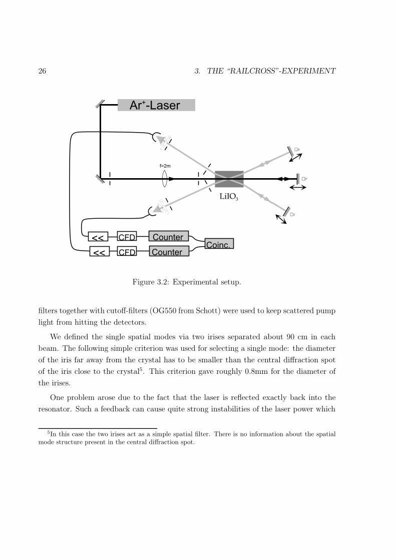
The experimental setup is shown in Fig. 3.2. An Ar+-laser (operated in UV at 351.1 nm
single frequency) pumps a nonlinear LiIO3-crystal. The two crystals which we employed
and the PDC-setup itself have been described in section 2.4. The overall distance from
the laser to the crystal was about 4 m in order to align the reflected pump beam as
best as possible. The power of the laser was typically between 100 and 300 mW. Behind
the crystal the laser was reflected from an UV-coated mirror (a COHERENT Ar+-laser
high reflector) back onto itself. The reflected laser beam passed a second time through
the crystal where it has a second possibility to create a photon pair. The other mirrors
that were used to reflect the downconverted light backwards were standard broadband
mirrors from TECOPTICS. All the mirrors were positioned with piezos with a resolution
finer than the optical wavelength. The signal- and idler-mirror were fixed within a
PICOMOTOR mirror mount (New Focus) that allowed a precise tilting of the mirrors.
Furthermore each mirror could be moved with µm resolution by DC-motors.
The wavelengths of the correlated photons were 632.8 nm for the signal and 788.7
nm for the idler beam. The former one was chosen because cheap HeNe-lasers for the
purpose of alignment (see below) were available at this wavelength. 5nm-interference
26 3. THE “RAILCROSS”-EXPERIMENT
!
"#
$$%&$$
%&
Figure 3.2: Experimental setup.
filters together with cutoff-filters (OG550 from Schott) were used to keep scattered pump
light from hitting the detectors.
We defined the single spatial modes via two irises separated about 90 cm in each
beam. The following simple criterion was used for selecting a single mode: the diameter
of the iris far away from the crystal has to be smaller than the central diffraction spot
of the iris close to the crystal5. This criterion gave roughly 0.8mm for the diameter of
the irises.
One problem arose due to the fact that the laser is reflected exactly back into the
resonator. Such a feedback can cause quite strong instabilities of the laser power which
5In this case the two irises act as a simple spatial filter. There is no information about the spatialmode structure present in the central diffraction spot.

3. THE “RAILCROSS”-EXPERIMENT 27
was observed actually. We were unable to reproducibly determine the optimal exper-
imental conditions. However it seemed that generally the fluctuations became larger
with increasing laser power. As a general rule, we had no instability problems when the
maximum laser power was about 100 mW.
Fig. 3.3 shows a photograph of our experimental arrangement. We used different
lasers to indicate the modes involved .
3.3.2 Detection and data acquisition
The essential point in our detection system was the capability to register single photons.
This cannot be done with ordinary photodiodes. The typical power of PDC emitted into
a specific mode, was about 10−14W.
In our experiment we used therefore avalanche-photodiodes operating in the Geiger-
mode, that is we applied a voltage that was about 20–25 V above the breakdown voltage.
A photon impinging on the active area causes with a high probability (typically > 50%)
an electron avalanche. This pulse has a fast rise time of about 0.5 ns and therefore the
detection time can be measured quite accurately. Peltier elements cool the detectors
down to about −30 or −40 in order to reduce the dark count rate from several thou-
sands per second down to a few hundreds per second. Several µsec are needed to quench
the avalanche again and to make the detector sensitive for the next photon. Therefore
the maximum count rate of a typical detectors is about 200000 counts/sec before it
saturates. For more details of the detector see appendix B and [Denifl93a].
After detection the pulses were amplified (e.g. VT120 A of EG&G), pulse-shaped in a
constant fraction discriminator (e.g. Tennelec model TC454) and then send to counters.
Additionally the pulses from the signal and idler detectors were both fed into a time
to amplitude converter (Tennelec model TC864) that serves as a coincidence counter.
Pulses coming within a coincidence window of typically 5 ns were counted as coincident.
We also used QUAD 4-input logic units (EG&G) as coincidence counters. As counters
we employed a TC512 dual counters of Tennelec and a 4-fold counter EG&G model 974.
All the count rates were recorded by a personal computer that also controlled the piezos
and DC-motors used to move the mirrors.

28 3. THE “RAILCROSS”-EXPERIMENT
Figure 3.3: Photograph of the experimental arrangement: Lasers with different colorswere used to indicate the various modes involved.
3. THE “RAILCROSS”-EXPERIMENT 29
3.3.3 Alignment of the experiment
The aligning procedure in our experiment basically was quite simple:
1. Adjust the pump mirror to send the pump beam back into itself. This could be
done best by placing several irises within the pump beam to define the direction.
Then the reflected pump beam can be centered onto these irises. The accuracy
possible with this method was better than 0.5mrad.
2. Adjust the signal- and idler-detectors (with open iris) )for maximum singles- and
coincidence count rates.
3. Block signal- and idler-mirror.
4. Close the irises until the count rates decrease to about the half.
5. Adjust the irises to optimize again singles- and coincidence-count rates.
6. Block the pump mirror and unblock signal- and idler-mirror.
7. Optimize signal- and idler mirror for maximum singles- and coincidence count
rates.
8. Repeat steps 3 -7 until the diameter of the irises is as small as possible or the count
rates become to low for further adjustment.
With this procedure we tried to optimize the “effective efficiency” of the detection
process. A good figure of merit is the ratio of the coincidence count rate divided by
the single count rate6. By optimizing it we ensure that both detectors look into the
right directions. In theory the upper limit of this ratio is determined by the quantum
efficiency of the detectors and the transmission of the various optical components before
the detectors (interference filters, lens, cutoff filters,...). This should give for the ratio
a value of about 10%. In practice, for our best alignment we could achieve a visibility
6This method also provides a means to estimate the efficiency of single-photon detectors [Klyshko80a,Rarity87a]

30 3. THE “RAILCROSS”-EXPERIMENT
of about 1% which is clearly below this value. One reason could be the remaining
divergency of the pump beam in combination with the small aperture sizes which results
in additional losses. In [Kwiat93g] it is shown that one must employ irises of at least 30
times the pump divergence angle in order to keep this kind of losses below 2%.
Some work has been invested in order to improve this aligning procedure. In one
attempt we used spatial filters in front of the signal and idler detectors in order to define
a single mode as good as possible. Additionally we put a beam expander into the pump
beam in order to better obtain a plane wave input beam. The motivation behind these
attempts was that the experiment should work best with well defined plane waves.
Another idea was the use of single mode fibers to select out a single mode and to
guide it directly to the detector7. In all those schemes the alignment was very difficult
and it was not possible to get interference with high visibility. This was mostly due to
the fact that we were not able to couple the downconverted light which goes via the
mirrors efficiently into the fiber (or the spatial filter) efficiently.
3.3.4 Stimulated downconversion
We could simplify the alignment procedure very much by using stimulated PDC. This
effect is basically the classical counterpart of the the spontaneous PDC8. One sends a
coherent laser beam (here a HeNe-laser) into the crystal. The mode has to match exactly
the mode of the downconverted light with the same frequency. In this case nonlinear
mixing of the HeNe-laser and the pump laser takes place and both the signal and the
conjugate idler count rate will increase. This effect depends critically on the spatial
overlap of the laser mode and the mode of the downconverted light.
Fig. 3.4 shows how we used the stimulated process in our setup. The HeNe-laser
was coupled into the signal mode by moving a mirror into the beam path in front of the
detector. The laser now goes through the crystal and is reflected at the signal mirror.
7An advantage of fibers was the availability of detectors with very low dark count rate (30 counts/secversus 300counts/sec with normal detectors). Therefore we used for the later experiments fiber detectorsin combination with multimode fibers.
8Analogously the spontaneous PDC can also be interpreted as induced by the vacuum fluctuations.

3. THE “RAILCROSS”-EXPERIMENT 31
'(
Figure 3.4: Stimulated PDC to align the experiment
Perfect overlap of the laser with the right signal mode could enhance the intensity of the
downconverted light9 by a factor of more than 100.
The stimulated downconversion allowed us to modify our alignment procedure in the
following way:
1. Align pump beam and signal and idler detectors in the same way as described
above. Now place the different irises into the signal- and idler-mode. Close the
irises and optimize their position using singles and coincidence count rates.
2. Send the HeNe-laser exactly in the middle trough the irises into the crystal.
3. Block the idler mirror.
4. If the mirror is in the right position the idler count rate increase very much due
to the stimulated downconversion process.
9This could be observed best in the idler singles count rate. The signal singles rate could not beobserved because the signal detector had to be blocked to protect it against the light from the HeNe-laserthat shines essentially into the same mode

32 3. THE “RAILCROSS”-EXPERIMENT
5. Determine whether the reflected HeNe-beam goes straight through the middle of
the irises.
6. If this is no the case repeat the steps 3 - 7.
7. Unblock the idler mirror and block signal- and pump mirror.
8. Adjust the idler-mirror again on the idler count rate.
This procedure provided us with a quite reliable method to align our interferometer.
The light generated by stimulated PDC can be described by a coherent state. There-
fore in the arrangement described above it should be possible to observe interference
between the direct and the reflected idler beam. An experiment has been carried out to
confirm this. First the signal mirror (or the idler mirror) is moved away to remove any
interference between the spontaneous photon pairs (see next section).
Due to the coherent nature of the stimulated downconversion one still can see a
modulation of the idler count rate upon moving the mirrors. The period is given by
the signal or idler wavelength depending on which mirror is moved. This phase de-
pendence is similar as for the case of spontaneous PDC. However the interference here
is completely classical in its nature. Related experiments already have been reported
in [Wu85a,Ou90e]. The complete theory is described in [Ou90e]. The result for the
interference visibility can be written in the following form:
VIS =nst
nst + nsp=
nstnsp
1 + nstnsp
Here nst and nsp are the number of stimulated and spontaneous photons resoectively
emitted into idler mode. As long as nst nsp the visibility approaches 1. But if the
intensity of the laser becomes so low that nst < nsp VIS decreases to zero Fig.3.5 shows
a good agreement with the theory if one normalizes the max visibility to about 82%.
Better alignment should make it possible to increase this value.
This behavior can be understood easily. Only the stimulated photons can contribute
to interference because the spontaneous idler photons are always created in pairs.As
3. THE “RAILCROSS”-EXPERIMENT 33
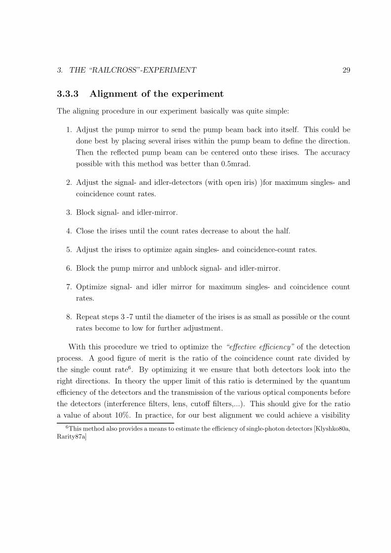
Figure 3.5: The visibility of stimulated interference in dependence on the ratio nstnsp
. This
ratio determines the indistinguishability of the photons detected at the idler detectorand therefore the contrast of the interference
explained in the second chapter these pairs are tightly correlated in time. Because
the signal mirror was moved away one can in principle identify the path of the idler
photon and no interference is possible. On the other hand for the stimulated photons no
information about the path is available because there is no correlation in time between
idler and signal beam. In other words the stimulated photons can interfere whereas the
spontaneously created photons just produce background.
3.4 Results and discussion
Now we present experimental data that verify the theoretical predictions made above.
First we had to equalize the distances of the signal- and idler mirror from the crystal.
The required accuracy is given by the coherence length of the photons registered by the
detectors (see the first section of this chapter). We established interference by performing
search scans using the DC-motors mounted at the mirrors. In such scans we used typical
steps of 10–20µm. Interference shows up in such an experiment as a strong broadening

34 3. THE “RAILCROSS”-EXPERIMENT
in the scattering of the different count rates (Fig. 3.6).
Figure 3.6: A typical coarse scan to find the region with maximal interference. Thewidth of the distribution is a means to determine the coherence length of the photons.The full line serves just as a guide for the eye.
Such coarse scans provided a good method to estimate the coherence length of the
downconverted light as measured by the detectors. The width of the coarse scan distri-
bution gave us this information. From Fig. 3.6 we estimated that the coherence length
is about 270µm10. This result corresponds to a effective FWHM-bandwidth of the PDC-
light of about 1.5nm which is much lower than the bandwidth of the interference filters
(5nm). To understand this outcome one must take into account the finite iris size (diam-
eter ≈ 0.8mm, distance ≈ 90cm from the crystal). A geometrical consideration shows
immediately that really the irises limit the spectrum to a bandwidth of roughly 1.6nm.
From the coarse scan we could find the maximum contrast of the interference pattern.
The fine details of these fringes could be resolved by moving the mirrors with the piezos.
Every data set from such a fine scan was evaluated by subtracting the background
10In a later experiment (see chapter 5.3) we made a much more careful determination of the coherencelength. We performed fine scans along the whole coherence profile. The results there agreed quitereasonable with the value obtained here.

3. THE “RAILCROSS”-EXPERIMENT 35
and fitting it to a cosine function with mean value, visibility, phase and wavelength
as parameters. Typical results (with that interference filters) for the visibility were
about 50% for the idler, 17% for the signal and 85% for the coincidences. We ascribe
this difference to the fact that the signal beam leaves the crystal under a smaller angle
because of its lower wavelength. Therefore the signal detector sees a larger volume
inside the crystal and thus a higher (non-interfering) background count rate. Later we
performed scans with narrow bandwidth interference filters where the difference was
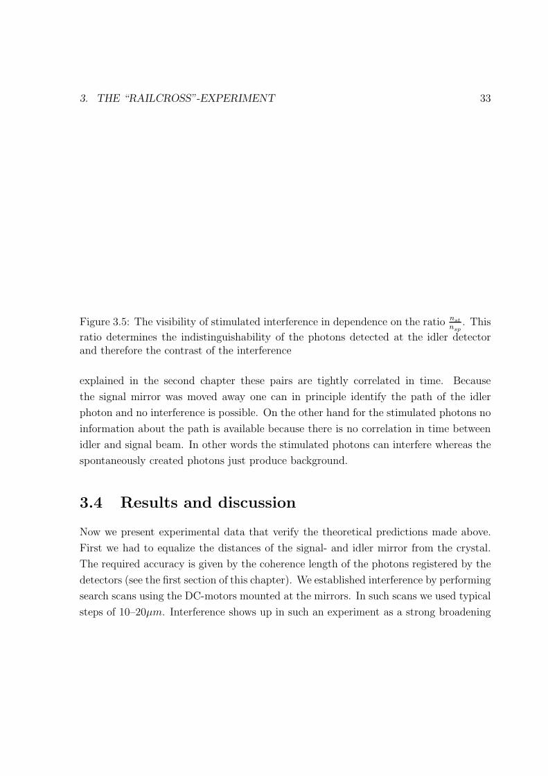
much smaller. Fig.3.7 shows the idler fringes obtained if one moves alternatively signal-,
idler- or pump-mirror. In agreement with Eq.(3.4) the fringe period was given by half
the wavelength of the beam whose mirror was scanned. The quantitative discrepancy
was due to drift of the mirror mounts. Higher mean count rates in the pump mirror
scan were owing only to the different laser power used in this particular measurement.
The results of Fig. 3.7 clearly show that all three mirrors together define the boundary
condition for emission of the idler and hence also for the signal photon.
Fig. 3.8 shows signal count rate, the idler count rate and the coincidence count rate
as measured as a function of the idler mirror position. All three measured curves varied
in the same way both in period and phase. This is again a consequence of Eq.3.4 and
thus of the fact that the mirror positions define the boundary condition for emission of
the photon pair in both modes. This result supports also the interpretation, that our
experimental arrangement allowed the manipulation of the creation of the photon-pair
itself. Especially a minimum must be interpreted as suppression of the downconversion
process, whereas a maximum corresponds to an enhancement.
This is demonstrated even more strikingly when the signal and the idler mirror are
translated simultaneously in the same direction. Using the phase matching condition one
can convert the signal- and idler-mirror displacement into an equivalent pump-mirror
displacement. This goes as follows. From eq.(3.4) one sees that a phase shift ∆φs+∆φi
corresponds to a phase shift ∆φp of the pump:
∆φs +∆φi ≡ ∆φp
By substituting∆x(s,i,p)
λ(s,i,p)for ∆φ(s,i,p) on both sides we get
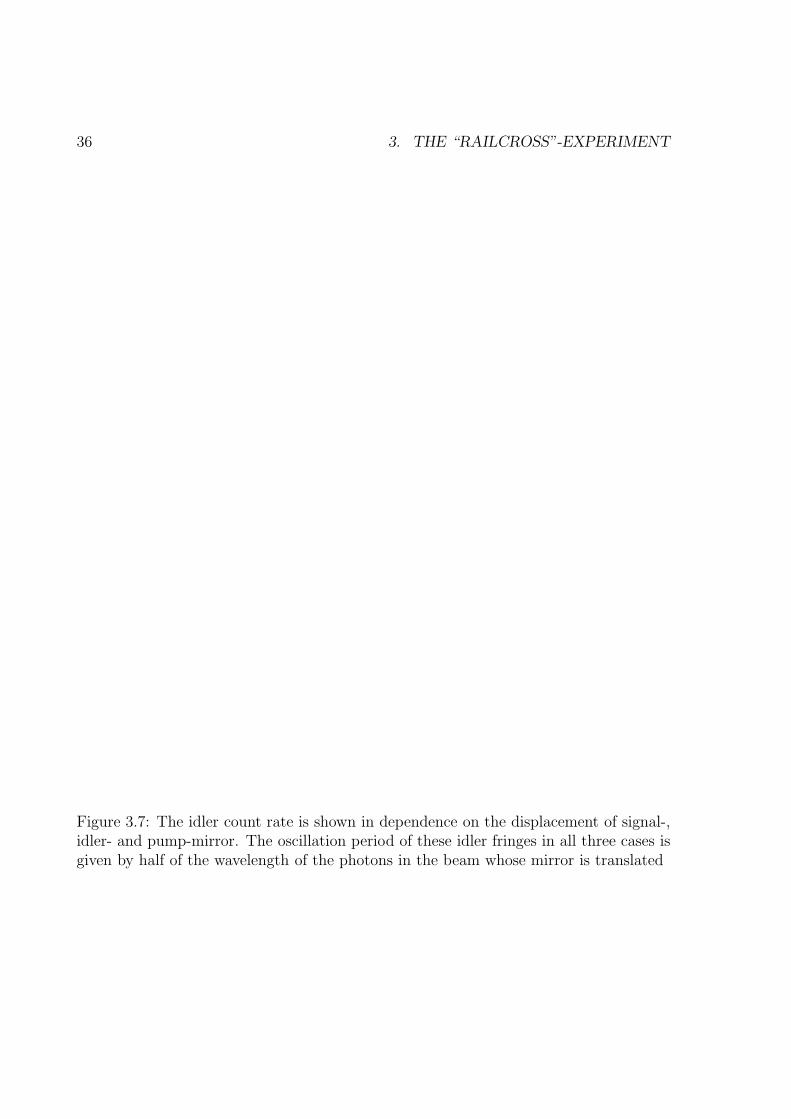
36 3. THE “RAILCROSS”-EXPERIMENT
Figure 3.7: The idler count rate is shown in dependence on the displacement of signal-,idler- and pump-mirror. The oscillation period of these idler fringes in all three cases isgiven by half of the wavelength of the photons in the beam whose mirror is translated

3. THE “RAILCROSS”-EXPERIMENT 37
Figure 3.8: Simultaneous measurement of signal count rate, idler count rate and coinci-dence count rate as a function of the displacement of the idler mirror.

38 3. THE “RAILCROSS”-EXPERIMENT
Figure 3.9: Measurement of idler count rate when both signal and idler mirror are trans-lated simultaneously. The abscissa represents a weighted sum of these displacements andit corresponds to an equivalent displacement of the pump mirror.
(∆xs
λs
+∆xi
λi
)λp ≡ ∆xp
Now we can apply energy conservation (see chapter 2.3) ( 1λs
+ 1λi
= 1λp) and we get:
λi
λi + λs
∆xs +λs
λi + λs
∆xi ≡ ∆xp (3.11)
Thus the idler count rate, measured as a function of that quantity (Fig. 3.9), varies
with a period of half the pump wavelength. These results show that it is only the sum
of the phases experienced by signal and idler which controls the emission of the photon
pair. Due to the entangled nature of the two-photon state neither signal nor idler enjoy
a well defined phase on their own because neither of them is in a pure state. Any phase
shift applied on either photon is really a phase shift acting on the joint product state of
both photons.
In order to state this even clearer we performed the following experiment. In any

3. THE “RAILCROSS”-EXPERIMENT 39
usual Mach-Zehnder (or Michelson) interferometer a mirror displacement (e.g., to in-
crease the path length L1) in one of the arms can only be compensated by moving the
mirror in the other arm in the same direction (that means, increase the path length L2
too). This behavior is due to the dependence of the interference pattern on the difference
φ1 − φ2 ∼ L1 −L2 of the two path lengths. This statement applies as well, if one makes
a displacement of the mirror by the order of the coherence length of the light to remove
interference. The fringes only can be restored by moving the other mirror by the same
amount in the same direction.
A two-photon interferometer works the other way round. The energy entanglement
is a inherent property of the correlated photon pairs. Therefore any interferometric
experiment employing these photons shows an interference pattern depending on the
sum φs + φi of the signal-and idler-phase. According to eq.(3.4) this statement is also
valid in our experiment. Consequently moving, for instance, the signal mirror can only
be compensated by moving the idler mirror into the opposite direction and vice versa.
However if we move the signal mirror by an amount of the order of the coherence length,
we can undo the resulting loss of interference only by moving the idler mirror in the
same direction.
This behavior is totally against intuition. Fig. 3.10 demonstrates the latter conclu-
sion. Two coarse scans (recorded in the same way as described on page 34) with the
signal mirror are shown.
Between both the idler mirror was translated by 1mm, which is about four times
the coherence length. In fact the maximum of the lower trace is shifted into the same
direction. Fig. 3.11 on the other hand depicts the situation if we look directly at the
behavior of the phases. The upper part shows the idler count rate if we first move the
signal mirror by a certain distance and afterwards the idler mirror by the same amount
in the opposite direction. It clearly can be seen that in second half the phase of the
modulation goes backwards that means here we have compensation. The lower trace
illustrates the other case. If we move the mirrors in the same direction, the modulation
does not reverse11.
11Note that in both cases the second part of the traces shows a slightly faster modulation. As alreadyexplained (Fig. 3.7) the period of the modulation is given by the wavelength of the light ascribed to
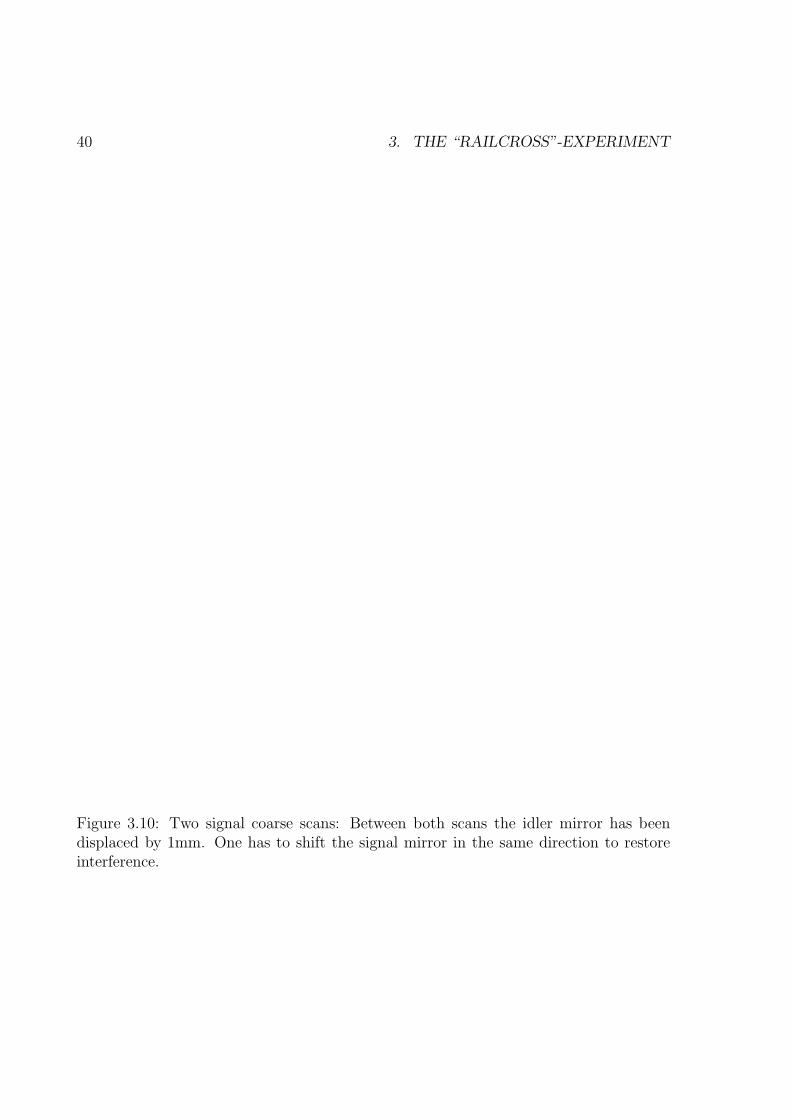
40 3. THE “RAILCROSS”-EXPERIMENT
Figure 3.10: Two signal coarse scans: Between both scans the idler mirror has beendisplaced by 1mm. One has to shift the signal mirror in the same direction to restoreinterference.
3. THE “RAILCROSS”-EXPERIMENT 41
Figure 3.11: Dependence on the sum of signal- and idler-phase: a) A shift of the signalmirror can only be compensated by moving the idler mirror into the opposite directionb) If one moves both mirrors in the same direction the phases add.
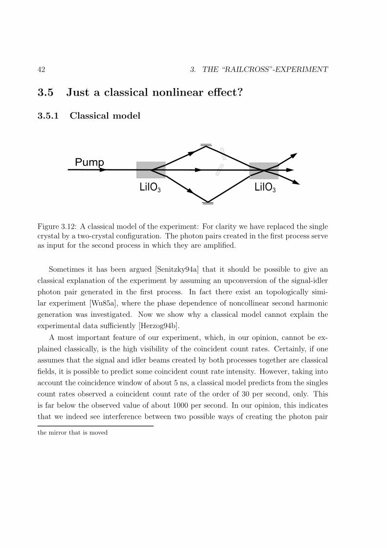
42 3. THE “RAILCROSS”-EXPERIMENT
3.5 Just a classical nonlinear effect?
3.5.1 Classical model
Figure 3.12: A classical model of the experiment: For clarity we have replaced the singlecrystal by a two-crystal configuration. The photon pairs created in the first process serveas input for the second process in which they are amplified.
Sometimes it has been argued [Senitzky94a] that it should be possible to give an
classical explanation of the experiment by assuming an upconversion of the signal-idler
photon pair generated in the first process. In fact there exist an topologically simi-
lar experiment [Wu85a], where the phase dependence of noncollinear second harmonic
generation was investigated. Now we show why a classical model cannot explain the
experimental data sufficiently [Herzog94b].
A most important feature of our experiment, which, in our opinion, cannot be ex-
plained classically, is the high visibility of the coincident count rates. Certainly, if one
assumes that the signal and idler beams created by both processes together are classical
fields, it is possible to predict some coincident count rate intensity. However, taking into
account the coincidence window of about 5 ns, a classical model predicts from the singles
count rates observed a coincident count rate of the order of 30 per second, only. This
is far below the observed value of about 1000 per second. In our opinion, this indicates
that we indeed see interference between two possible ways of creating the photon pair
the mirror that is moved
3. THE “RAILCROSS”-EXPERIMENT 43
as an entity. The only way to achieve a classical explanation were to assume that the
signal and idler beams are emitted as coincident pulses with a width comparable to or
smaller than the coincidence time resolution. Yet, we argue, such a structure of random
pulses is unphysical in stationary experiments like ours.
This argument is valid for every experiment using PDC including the first experiment
by Burnham and Weinberg [Burnham70a]. We also want to point out in this section
that, while it is possible to give a classical explanation of certain aspects of the observed
interference in our experiment, there cannot be success to capture the whole set of our
data in a single consistent scheme. First we carry out a quantitative estimation of the
visibility that we can expect from a classical viewpoint.
Following Boyd [Boyd92a]12 the basic equations of parametric amplification are given
(note the definition of E: E(t) := Ee−iωt + c.c.) by:
dEi
dz= κiE
s (3.12)
dEs
dz= κsE
i (3.13)
with the constants :
κi =8πiω2
i deffkic
2Ep κs =
8πiω2sdeff
ksc2
Ep (3.14)
Here deff is the effective nonlinearity of the crystal, αi and αs are absorption coeffi-
cients. Ei, Es and Ep are signal-, idler- and pump-field. Furthermore we have assumed
for simplicity perfect phase matching, that is ∆k = kp − ks − ki ≈ 0.
We suppose that both the signal- and idler-photons created in the first crystal (that
means the first process in the real experiment) are injected as classical input fields with
(complex) amplitudes Ei(0) and Es(0) in the second crystal. The solution to these
12Within this section we use Gaussian units.Furthermore we make use of the “slowly varying envelope”approximation in combination with a nondepleted pump and negligible absorption

44 3. THE “RAILCROSS”-EXPERIMENT
equations then can be derived with standard methods (see [Boyd]) and we get after the
second crystal at z=L:
Ei(L) = Ei(0) cosh(√κiκ
sL) +
κi√κiκ
s
E s (0) sinh(
√κiκ
sL) (3.15)
Es(L) = Es(0) cosh(√κiκ
sL) +
κs√κiκ
s
E i (0) sinh(
√κiκ
sL) (3.16)
Using κs√κiκ
s
=√
ωinsωsni
Ep(0)√|Ep(0)|2
=√
ωinsωsni
eiφp one can see that this equation displays
interference with the same phase dependence as predicted by the quantum mechanical
model. The visibility can be easily calculated with the result:
V is =Max −Min
Max +Min
=2|Ei(0)||Es(0)|
√ωinsωsni
sinh(√κiκ
sL) cosh(
√κiκ
sL)
|Ei(0)|2 cosh2(√κiκ
sL) + |Es(0)|2 ωins
ωsnisinh2(
√κiκ
sL)
(3.17)
For a better understanding of this result we redefine the field variables in the following
way:
Al :=
√nl
ωl
El l = p, s, i (3.18)
This gives for the intensity:
Il =Pl
A=
nlc
2π|El|2 =
c
2πωl|Al|2 (3.19)
which means that : Ns/i = |As/i(0)|2 is proportional to the input photon flux itself at
ωs/i. Furthermore we rewrite√κiκ
s =
8πωiωsdeff√kiksc
2|Ep| =: C|Ep|. Now the visibility can
be written as:
V is =2√NiNl sinh(C|Ep|L) cosh(C|Ep|L)
Ni cosh2(C|Ep|L) +Ns sinh
2(C|Ep|)(3.20)
This result shows that the visibility depends very strongly on the pump power within
our classical model. If we assume degeneracy between signal and idler (λs = λi → ns =
3. THE “RAILCROSS”-EXPERIMENT 45
ni) and with Ns = Ni (as it is the case for PDC) we can achieve a visibility of up to
100% for infinite pump power or interaction length.
For the opposite case, C|Ep|L 1 the result is:
V is ≈ 2√κiκ
sL = 2C|Ep|L 1 (3.21)
Now we give an estimation for our experiment:
The relation between intensity and the electric field strength of a harmonic light field
reads as follows:
I =nc
2π|E|2
(n is the refractive index, I in ergcm2s
, c = 3× 10¹⁰ cms
and E in statvoltscm
≈ 3× 10⁴ Vm)
With I = 109 ergcm2 and n(λ = 351nm) = 1.8134 we get:
|E| = = 0.3398statvolt
cm= 1.0195× 10⁴ V
m
=⇒ κi = 0.4734m−1 κs = 0.5858m−1
With L = 1cm we get from eq.(3.21):
V is = ≈ 1% (3.22)
This value is much smaller than the visibility we was able to observe in our exper-
iment. There the order of magnitude was always between 40% and 60%. Fig. 3.13
shows the quantitative dependence of the visibility on the power of the pump laser as
predicted by the classical model for our experiment. To explain the observed data we
need a pump power that is about three orders of magnitude larger than actually used.
Moreover the observed visibility depends neither on the pump power nor on the length
of the crystal.
We have seen that our classical model cannot reproduce visibility in the first order
interference. That means it is possible to explain certain aspects of the experimental
data within a classical framework. However it is not possible to capture all aspects of
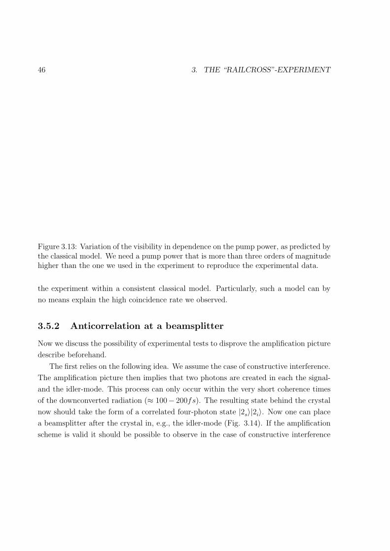
46 3. THE “RAILCROSS”-EXPERIMENT
Figure 3.13: Variation of the visibility in dependence on the pump power, as predicted bythe classical model. We need a pump power that is more than three orders of magnitudehigher than the one we used in the experiment to reproduce the experimental data.
the experiment within a consistent classical model. Particularly, such a model can by
no means explain the high coincidence rate we observed.
3.5.2 Anticorrelation at a beamsplitter
Now we discuss the possibility of experimental tests to disprove the amplification picture
describe beforehand.
The first relies on the following idea. We assume the case of constructive interference.
The amplification picture then implies that two photons are created in each the signal-
and the idler-mode. This process can only occur within the very short coherence times
of the downconverted radiation (≈ 100− 200fs). The resulting state behind the crystal
now should take the form of a correlated four-photon state |2s〉|2i〉. Now one can place
a beamsplitter after the crystal in, e.g., the idler-mode (Fig. 3.14). If the amplification
scheme is valid it should be possible to observe in the case of constructive interference

3. THE “RAILCROSS”-EXPERIMENT 47
!
)* !
Figure 3.14: Experimental setup to test the amplification picture: A beamsplitter isinserted in the idler mode. Coincidences Ns∧i1 and Ns∧i2 are counted between the signaldetector and each idler detector by using two TAC’. In addition we count the triplecoincidences Ns∧i1∧i2 by feeding one of the coincidences Ns∧i1together with the singlesof the other idler detector Ni2
into a logic-gate. In the case of parametric amplificationtriple-coincidences should occur.
triple coincidences between signal detector and the two outputs of the beamsplitter. In
fact this was not the case in our setup as we could show.
Any classical description would yield counting rates obeying the inequality [Grangier86a]:
α =Ns∧i1∧i2Ns
Ns∧i1Ns∧i2≥ 1 (3.23)
In an actual experiment, the different count rates were Ns = 46434/50s, Ns∧i1 =
380/50s and Ns∧i2 = 162/50s. 13. For the classical expected triple count rate it follows
from eq.(3.23) Ns∧i1∧i2Ns ≈ 1.3/50s. As described in Grangier86a, one can calculate α
with quantum mechanics and get α ≈ 0.004. This corresponds to a triple count rate of
about Ns∧i1∧i2Ns ≈ 0.006/50s that is much smaller than the classical one. This result
could be confirmed roughly in the experiment (1 triple coincidence within 15 data points
13We calibrated in a preceding experiment (by measuring the classical coincidences in a chaotic whitelight source)the different coincidence windows. We found that they were not equal. In order to get theworst case we therefore assumed in our the estimations the largest window (≈ 19ns).

48 3. THE “RAILCROSS”-EXPERIMENT
a 50 s each). Therefore we could rule out the amplification picture as an explanation for
our experiment 14
Another experimental test was proposed by [Zukowski95a]. It is one consequence
of the amplification picture that the resulting state behind the crystal depends on the
concrete mirror settings. In the case of destructive interference we have only a vacuum
state, whereas constructive interference implies, as explained above, a correlated 4 pho-
ton state The case between is the common two-photon state |1s〉|1i〉. The signal- and
idler-behind the crystal modes now are combined on another beamsplitter. Perfect tem-
poral and spatial overlap is necessary. The coincidences between the output modes of the
beamsplitter depend on the state sent in [Fearn89a]. If one sends exactly one photon in
each input of the beamsplitter the coincidences vanish completely [Hong87a, Mattle93a].
A measurement of the coincidence upon variation of the phases thus should show a mod-
ulation if the amplification picture is valid. Otherwise such a modulation should not
occur.
14Our result can serve only as an estimation for α. One needs some parameters, that are not reallyknown. The total number of photon pairs created within the crystal in direction to the detector is themost important one. In order to get this number one needs the collection efficiency of the detectorsthat is afflicted with a big error.

“...one should no more rack one’s brain aboutthe problem of whether something one cannotknow anything about exists all the same, thanabout the ancient question of how many angelsare able to sit on the point of a needle. But itseems to me that Einstein’s questions are ulti-mately always of this kind.”
O.Stern-W.Pauli to M.Born 1954
4 Welcher-Weg Experiments and
Quantum Eraser
4.1 Introduction
In every measurement process one makes usually the implicit assumption that the mea-
suring device can be treated classically. The reason is that it concerns a macroscopic
apparatus with a solid pointer that gives us more or less a unambiguous result. The pos-
sibility to do this simplifies life in physics greatly. However one always has to be aware
that the measurement process, that manifests the transition from the quantum world to
the classical world, is not nearly as well understood as one might think [Zurek91a].
There exist situations where the assumption of a classical measurement device is not
valid. In order to get correct predictions in these cases, it is necessary to include the
measurement apparatus in the quantum mechanical treatment. The “Welcher-Weg”
(which-path) and “Quantum Eraser” experiments described in this and in the next
chapter are just such situations.
49

50 4. WELCHER-WEG EXPERIMENTS AND QUANTUM ERASER
4.2 Welcher-Weg information and loss of interfer-
ence
In the first chapter it has been argued already, that interference (e.g. in the double slit
experiment) is the most fundamental phenomenon in quantum mechanics. Although a
quantum system can reveal both wave-like (interference) and particle-like behavior (pas-
sage through only one of the two slits), it turns out that it is impossible to obtain both
interference and complete which-path information in a single experiment. According to
the Feynman rules, as discussed in chapter 1, it is only possible to see interference if the
two path are indistinguishable. Any attempt to extract which-path information from
such an interference experiment will degrade the contrast of the fringe pattern — if one
can fully determine the path, then there is no interference at all.
To describe situations like this correctly Niels Bohr introduced the notion of comple-
mentarity that distinguishes the realm of quantum physics from the world of classical
physics.(see also the quotation on page 3) 1. There exist classes of experiments which
are mutual exclusive, that means one cannot perform both simultaneously on a quan-
tum system. One class displays wavelike properties in the form of interference. Another
one gives information about the behavior as a particle in the form of which-path infor-
mation. Both setups are complementary in the sense that together they exhausts all
knowledge that can be obtained about the object of interest. Furthermore they are also
complementary in the sense that they exclude each other, i.e. both experiments cannot
be carried out simultaneously on the same object.
What do we mean by a which-path measurement? First let us introduce some his-
torical examples. Afterwards we turn to a general discussion of the problem.
The classic example, that throws more light upon the problem, is the famous recoiling
slit gedanken experiment [Schilpp49a] first introduced by Einstein2. In order to prove
1In fact, complementarity is a much more general concept. In the words of Scully et al. [Scully91a]:“Two observables are complementary if precise knowledge of one of them implies that all possible out-comes of measuring the other are equally probable.“ This concept applies to any pair of non commutatingobservables, e.g. different components of spin or angular momentum. However in the phenomenon ofinterference the consequences of complementarity are most amazing
2during the 5th Physical Conference of the Solvay Institute in Brussels, October 1927
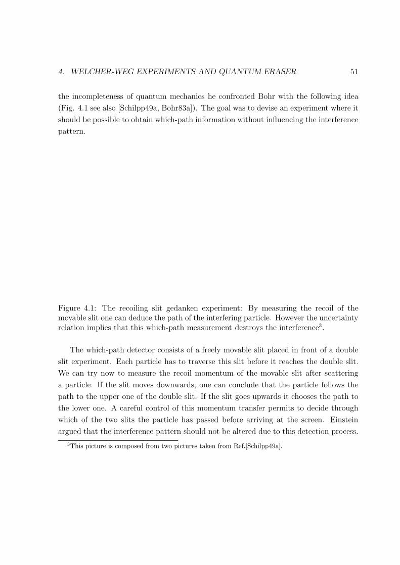
4. WELCHER-WEG EXPERIMENTS AND QUANTUM ERASER 51
the incompleteness of quantum mechanics he confronted Bohr with the following idea
(Fig. 4.1 see also [Schilpp49a, Bohr83a]). The goal was to devise an experiment where it
should be possible to obtain which-path information without influencing the interference
pattern.
Figure 4.1: The recoiling slit gedanken experiment: By measuring the recoil of themovable slit one can deduce the path of the interfering particle. However the uncertaintyrelation implies that this which-path measurement destroys the interference3.
The which-path detector consists of a freely movable slit placed in front of a double
slit experiment. Each particle has to traverse this slit before it reaches the double slit.
We can try now to measure the recoil momentum of the movable slit after scattering
a particle. If the slit moves downwards, one can conclude that the particle follows the
path to the upper one of the double slit. If the slit goes upwards it chooses the path to
the lower one. A careful control of this momentum transfer permits to decide through
which of the two slits the particle has passed before arriving at the screen. Einstein
argued that the interference pattern should not be altered due to this detection process.
3This picture is composed from two pictures taken from Ref.[Schilpp49a].
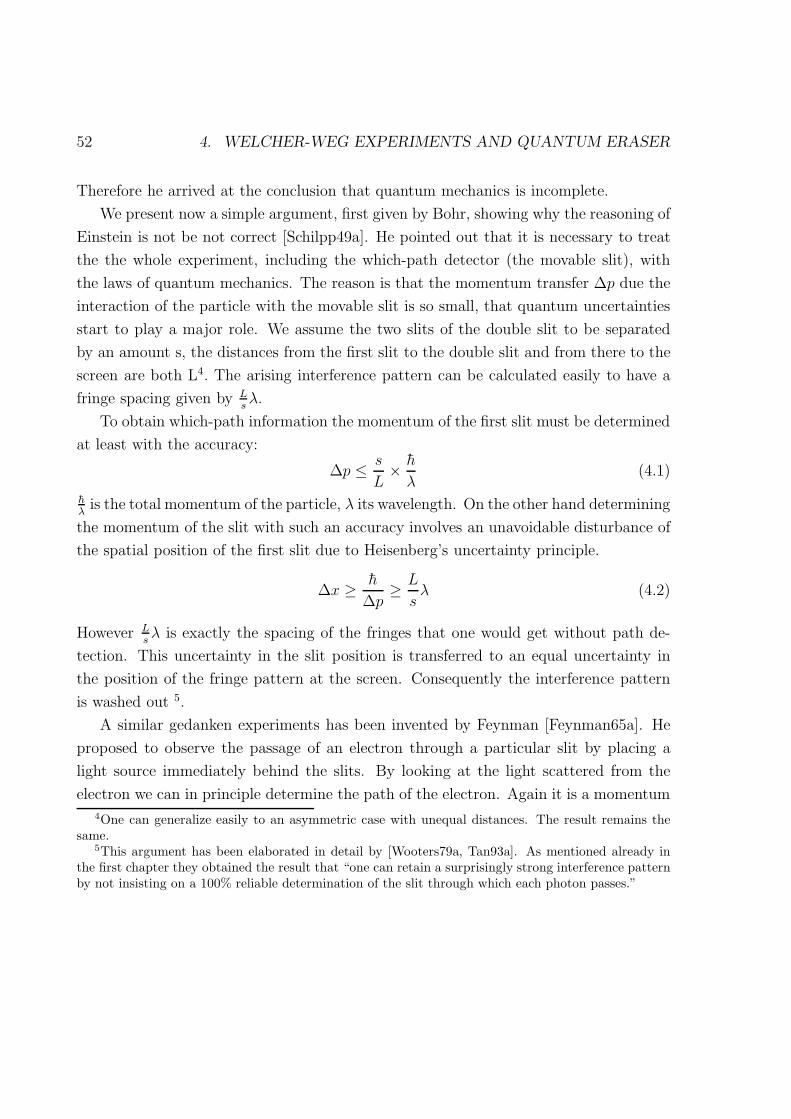
52 4. WELCHER-WEG EXPERIMENTS AND QUANTUM ERASER
Therefore he arrived at the conclusion that quantum mechanics is incomplete.
We present now a simple argument, first given by Bohr, showing why the reasoning of
Einstein is not be not correct [Schilpp49a]. He pointed out that it is necessary to treat
the the whole experiment, including the which-path detector (the movable slit), with
the laws of quantum mechanics. The reason is that the momentum transfer ∆p due the
interaction of the particle with the movable slit is so small, that quantum uncertainties
start to play a major role. We assume the two slits of the double slit to be separated
by an amount s, the distances from the first slit to the double slit and from there to the
screen are both L4. The arising interference pattern can be calculated easily to have a
fringe spacing given by Lsλ.
To obtain which-path information the momentum of the first slit must be determined
at least with the accuracy:
∆p ≤ s
L× h
λ(4.1)
hλis the total momentum of the particle, λ its wavelength. On the other hand determining
the momentum of the slit with such an accuracy involves an unavoidable disturbance of
the spatial position of the first slit due to Heisenberg’s uncertainty principle.
∆x ≥ h
∆p≥ L
sλ (4.2)
However Lsλ is exactly the spacing of the fringes that one would get without path de-
tection. This uncertainty in the slit position is transferred to an equal uncertainty in
the position of the fringe pattern at the screen. Consequently the interference pattern
is washed out 5.
A similar gedanken experiments has been invented by Feynman [Feynman65a]. He
proposed to observe the passage of an electron through a particular slit by placing a
light source immediately behind the slits. By looking at the light scattered from the
electron we can in principle determine the path of the electron. Again it is a momentum
4One can generalize easily to an asymmetric case with unequal distances. The result remains thesame.
5This argument has been elaborated in detail by [Wooters79a, Tan93a]. As mentioned already inthe first chapter they obtained the result that “one can retain a surprisingly strong interference patternby not insisting on a 100% reliable determination of the slit through which each photon passes.”
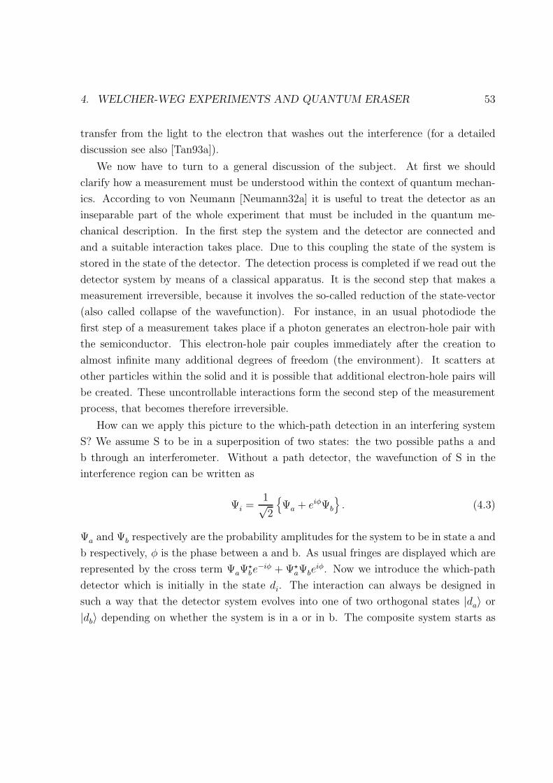
4. WELCHER-WEG EXPERIMENTS AND QUANTUM ERASER 53
transfer from the light to the electron that washes out the interference (for a detailed
discussion see also [Tan93a]).
We now have to turn to a general discussion of the subject. At first we should
clarify how a measurement must be understood within the context of quantum mechan-
ics. According to von Neumann [Neumann32a] it is useful to treat the detector as an
inseparable part of the whole experiment that must be included in the quantum me-
chanical description. In the first step the system and the detector are connected and
and a suitable interaction takes place. Due to this coupling the state of the system is
stored in the state of the detector. The detection process is completed if we read out the
detector system by means of a classical apparatus. It is the second step that makes a
measurement irreversible, because it involves the so-called reduction of the state-vector
(also called collapse of the wavefunction). For instance, in an usual photodiode the
first step of a measurement takes place if a photon generates an electron-hole pair with
the semiconductor. This electron-hole pair couples immediately after the creation to
almost infinite many additional degrees of freedom (the environment). It scatters at
other particles within the solid and it is possible that additional electron-hole pairs will
be created. These uncontrollable interactions form the second step of the measurement
process, that becomes therefore irreversible.
How can we apply this picture to the which-path detection in an interfering system
S? We assume S to be in a superposition of two states: the two possible paths a and
b through an interferometer. Without a path detector, the wavefunction of S in the
interference region can be written as
Ψi =1√2
Ψa + eiφΨb
. (4.3)
Ψa and Ψb respectively are the probability amplitudes for the system to be in state a and
b respectively, φ is the phase between a and b. As usual fringes are displayed which are
represented by the cross term ΨaΨ be−iφ + Ψ
aΨbeiφ. Now we introduce the which-path
detector which is initially in the state di. The interaction can always be designed in
such a way that the detector system evolves into one of two orthogonal states |da〉 or|db〉 depending on whether the system is in a or in b. The composite system starts as
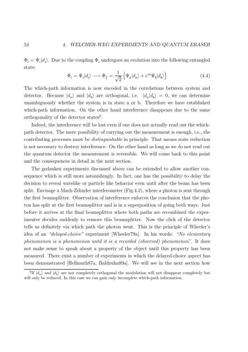
54 4. WELCHER-WEG EXPERIMENTS AND QUANTUM ERASER
Φi = Ψi|di〉. Due to the coupling Φi undergoes an evolution into the following entangled
state:
Φi = Ψi|di〉 −→ Φf =1√2
Ψa|da〉+ eiφΨb|db〉
(4.4)
The which-path information is now encoded in the correlations between system and
detector. Because |da〉 and |db〉 are orthogonal, i.e. 〈da|db〉 = 0, we can determine
unambiguously whether the system is in state a or b. Therefore we have established
which-path information. On the other hand interference disappears due to the same
orthogonality of the detector states6.
Indeed, the interference will be lost even if one does not actually read out the which-
path detector. The mere possibility of carrying out the measurement is enough, i.e., the
contributing processes must be distinguishable in principle. That means state reduction
is not necessary to destroy interference. On the other hand as long as we do not read out
the quantum detector the measurement is reversible. We will come back to this point
and the consequences in detail in the next section.
The gedanken experiments discussed above can be extended to allow another con-
sequence which is still more astonishingly. In fact, one has the possibility to delay the
decision to reveal wavelike or particle like behavior even until after the beam has been
split. Envisage a Mach-Zehnder interferometer (Fig.4.2), where a photon is sent through
the first beamsplitter. Observation of interference enforces the conclusion that the pho-
ton has split at the first beamsplitter and is in a superposition of going both ways. Just
before it arrives at the final beamsplitter where both paths are recombined the exper-
imenter decides suddenly to remove this beamsplitter. Now the click of the detector
tells us definitely via which path the photon went. This is the principle of Wheeler’s
idea of an “delayed-choice” experiment [Wheeler79a]. In his words: “No elementary
phenomenon is a phenomenon until it is a recorded (observed) phenomenon”. It does
not make sense to speak about a property of the object until this property has been
measured. There exist a number of experiments in which the delayed-choice aspect has
been demonstrated [Hellmuth87a, Baldzuhn89a]. We will see in the next section how
6If |da〉 and |db〉 are not completely orthogonal the modulation will not disappear completely butwill only be reduced. In this case we can gain only incomplete which-path information.

4. WELCHER-WEG EXPERIMENTS AND QUANTUM ERASER 55
Figure 4.2: The delayed choice gedankenexperiment invented by J. A. Wheeler: Thedecision whether to see interference or to obtain which-path information can be delayeduntil briefly before the photon arrives at the final beamsplitter (picture taken from[Wheeler83a??]).
one can extend the delayed-choice concept to become even more striking.
The examples that we have discussed up to now, suggests the following conclusion:
Which-path detection is always accompanied by an unavoidable disturbance of the mo-
mentum distribution that is responsible for the loss of interference. However one may
ask whether this picture is always true. Is a momentum transfer really necessary in
any case to destroy interference? There is an still ongoing discussion about this issue
[Scully91a, Englert94a, Storey94b]. In order to comprehend this problem better, let us
have a look at the following experiment proposed in [Scully91a]. There the authors claim
that under certain circumstances one must regard the loss of interference as arising from
the entanglement of the wave function of the interfering system with that of the mea-
surement apparatus. In these cases there does not take place any momentum transfer
from the which-path detector to the interfering system.
The basic setup is essentially is sketched in Fig. 4.3. It is basically the atom analogue

56 4. WELCHER-WEG EXPERIMENTS AND QUANTUM ERASER
to Young’s double-slit experiment. Coherent atoms beams illuminate two narrow slits
where the interference pattern that appears on the “screen” originates. The two beams
pass through two high-quality microwave cavities a and b, placed just before each slit.
The photon field there is assumed to be initially in the vacuum state. Before entering
the cavities a laser excites the atoms. The experiment can be arranged such that an
excited atom passing through a resonator emits with nearly 100% probability a photon
into the resonant cavity mode (for technical details see [Englert94b]). Then the photon
field inside the cavities provides which-path information. By testing in which cavity the
photon has been emitted, one is able in principle to determine which slit the atom has
traversed.
Figure 4.3: A two slit experiment with atoms excited by a laser. High-quality microwavecavities are placed in front of each slit to provide which-path information (picture takenfrom Ref. [Scully91a]).
Without the which-path detectors in use (e.g. laser does not excite the atoms), the
state of the atoms can be written in the form of eq.4.3:
Ψt =1√2
(Ψa + eiφΨb
)(4.5)
where φ is the phase difference between the two paths. |g〉A denotes the ground state

4. WELCHER-WEG EXPERIMENTS AND QUANTUM ERASER 57
of the atom, |e〉A the excited One gets the probability to register the atom at a certain
point on the screen by taking the squared modulus of this amplitude:
|Ψt|2 =1
2
|Ψa|2 + |Ψb|2 + eiφΨ
aΨb + e−iφΨaΨ b
(4.6)
The nonvanishing cross terms represent the usual interference pattern.
Next we introduce the which-path detector (i.e. the microwave cavities) One can do
this by turning on the laser to excite the atoms from |g〉 to |e〉. After emitting a photon
into the cavity, it ends up again in the ground state. Now the state of the interfering
particle becomes entangled with the state of the photon field in the two cavities:
Ψt −→1√2
Ψa|a〉P + eiφΨb|b〉P
|g〉A. (4.7)
where |a〉P denotes a state with the photon in cavity a and |b〉P the state with the photon
in cavity b. The existence of such states has not yet been demonstrated experimentally
but the realization seems to be feasible although it may be quite difficult in practice
[Haroche92a, Scully91a]. Calculating the interference pattern gives in this case:
|Ψt|2 =1
2
[|Ψa|2 + |Ψb|2 + eiφΨ
aΨb P 〈a|b〉P + e−iφΨaΨ b P 〈a|b〉P
]. (4.8)
Because the two possible states of the photon field (cavity a or cavity b) are orthogo-
nal, P 〈a|b〉P = 0, the two possible paths are distinguishable and the interference terms
disappear7. Again which-path information is stored in the correlation of the atom-cavity
system as emphasized by the entangled character of eq.(4.7). It is important to stress
one more time that actually it is not necessary to read out the which-path detector. It
is enough if one has the mere possibility to perform this measurement, i.e. as long as
the two paths are distinguishable in principle.
At present there is a discussion about the question whether this scheme provides the
possibility to obtain which-path information without disturbing the atom’s momentum.
To be more specific all the schemes proposed before made use of the uncertainty relations
7In general the visibility of the modulation pattern is reduced by a factor given by the scalar productof the two cavity states P 〈a|b〉P . A more general discussion of this point has been given in [Tan93a]

58 4. WELCHER-WEG EXPERIMENTS AND QUANTUM ERASER
to demonstrate complementarity. The conclusion seems obvious that the latter is a result
of the uncertainty relation. Scully et al. [Scully91a, Englert94a] claim that their which-
path detection scheme does not involve any momentum transfer between detector and
particle. Therefore they regard complementarity as a principle that is more fundamental
and the Heisenberg relation as a consequence. In fact they were able to show explicitly
[Englert94b] that during the passage through the cavities the atomic wave function does
not change considerably.
On the other hand Storey et al. [Storey94b] recently came up with a general argument
which they claim proves that any which-path measurement involves momentum transfer
to the interfering system. The resulting disturbance of the momentum distribution is
responsible for the loss of interference. The physical mechanism causing this momentum
transfer is not yet clear.
Nevertheless even if the atom has after the interaction the same momentum and the
same energy and the same momentum as before, during the coupling the atom feels a
potential which causes a overall phase shift of the wavefunction. The sign of the interac-
tion energy depends on the polarization of the atom with respect to the resonator field.
For a positive (negative) interaction energy the cavity field acts as a potential barrier
(well) that slows down (speeds up) the atom. After leaving the cavity the atom has its
initial value but it is displaced forward (backward). In [Englert90a] it was shown that in
the micromaser path detector the atom wavefunction gets a longitudinal displacement
by an amount of ±π2depending on the sign of the interaction energy. On the other
hand the atoms sent in the cavity are excited to the upper level that can be seen as a
superposition containing all the polarizations. Therefore the phase of the atomic wave
function is no longer well defined after leaving the cavity and the interference pattern is
washed out.
Stern et al. [Stern90a] have generally shown that such a randomization of the phase
takes place whenever the interfering system couples to an external environment. A
which-path detector is also an example for such a system. It happens even if altogether
no net energy- or momentum transfer occurs. The micromaser path detector is one

4. WELCHER-WEG EXPERIMENTS AND QUANTUM ERASER 59
example for this8. In the next chapter we present an experiment that demonstrates
which-path detection without any transfer of momentum.
4.3 The quantum eraser
The following question now becomes obvious: Is the loss of interference always an irre-
versible process or is it possible to restore interference? Indeed, Scully and Druhl pointed
out that one may get back the fringes if one manages it to “erase” the which-path infor-
mation simultaneously preserving the phase coherence [Scully82a]. Being more precise,
we have mentioned in the last section that the measurement process may be reversible.
This means we can remove the which-path information and recover interference, as long
as no decoherence effects destroy the correlation between detector and interfering sys-
tem. The loss of coherence becomes irreversible, if we couple our quantum detector to a
classical macroscopic apparatus to read it out. In the case of the micromaser detector,
this means detecting the photon within the cavity9.
How can we erase the which-path information without destroying the coherence effec-
tively? One has to perform actively a suitable measurement on the which-path detector.
In fact the detector system must be measured in a superposition of the two detector
states or with other words we choose a different base in which we carry out the detec-
tion. Finding the measuring system in such a state it does not deliver us with which-path
information. Interference may be regained by correlating the results of this measurement
with the detection of the initially interfering particle. Only for the subset of particles on
which we have performed that measurement explicitely we see interference again. This
is the physical concept of the so-called “Quantum Eraser”.
Furthermore, if the path information is not carried by the interfering system itself
but instead by a distinct which-path detector system, the decision of whether to read out
8Recently another scheme [Bryce95a] has been proposed in context with atom interferometry. Itmakes use of the concept of interaction free measurements[Elitzur93a, Kwiat95a]. There it is still moredifficult to see how any momentum transfer could be involved.
9Also the loss of the photon by dissipation is enough to destroy coherence. Quantum coherence is avery fragile object.
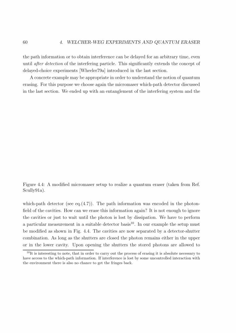
60 4. WELCHER-WEG EXPERIMENTS AND QUANTUM ERASER
the path information or to obtain interference can be delayed for an arbitrary time, even
until after detection of the interfering particle. This significantly extends the concept of
delayed-choice experiments [Wheeler79a] introduced in the last section.
A concrete example may be appropriate in order to understand the notion of quantum
erasing. For this purpose we choose again the micromaser which-path detector discussed
in the last section. We ended up with an entanglement of the interfering system and the
Figure 4.4: A modified micromaser setup to realize a quantum eraser (taken from Ref.Scully91a).
which-path detector (see eq.(4.7)). The path information was encoded in the photon-
field of the cavities. How can we erase this information again? It is not enough to ignore
the cavities or just to wait until the photon is lost by dissipation. We have to perform
a particular measurement in a suitable detector basis10. In our example the setup must
be modified as shown in Fig. 4.4. The cavities are now separated by a detector-shutter
combination. As long as the shutters are closed the photon remains either in the upper
or in the lower cavity. Upon opening the shutters the stored photons are allowed to
10It is interesting to note, that in order to carry out the process of erasing it is absolute necessary tohave access to the which-path information. If interference is lost by some uncontrolled interaction withthe environment there is also no chance to get the fringes back.

4. WELCHER-WEG EXPERIMENTS AND QUANTUM ERASER 61
interact with the photodetector wall.
To understand better what happens, we have to extend eq.(4.7) to include the new
detector system, which we model by a two-level system with ground state |d〉 and excited
state |e〉:Ψt =
1√2
Ψa|a〉+ eiφΨb|b〉
|d〉 (4.9)
Absorption of a photon excites the detector from state |d〉 to |e〉. After opening the
shutters it is more convenient to describe the photon field in a different basis. We define
symmetric and antisymmetric superpositions of the radiation fields contained in the
cavities:
|±〉P =1√2(|a〉P ± |b〉P ) . (4.10)
Only the symmetric state |+〉P can interact with the detector wall, for the antisymmetric
state the field distribution vanishes at the detector wall.
We also introduce symmetric and antisymmetric superpositions of the atomic wave-
functions, Ψ+ and Ψ−:
Ψ± =1√2
(Ψa ± eiΦΨb
). (4.11)
Note that these states carry explicitly the phase φ. We can rewrite the state of eq. (4.9)
and we obtain with closed shutters (no interaction field-detector):
Ψt =1√2
Ψ+|+〉P +Ψ−|−〉P
|g〉 (4.12)
Opening the shutters a photon found in state |+〉P causes a detector click whereas a
photon in state |−〉P does not because the |−〉 has a node at the position of the detector.
Afterwards we find the whole system in the state:
Ψt =1√2
Ψ+|0〉P |e〉+Ψ−|−〉P |g〉
. (4.13)
We now pick out exactly the detection events of the atom at the screen where we find
the detector excited (e.g. we project out the state Ψ+ for the atoms). This correlation
reveals again the original fringe pattern (the solid line in Fig. 4.4b) due to the fact
that both Ψ+ and ψ− depend on the phase φ. On the other hand, we can also correlate
62 4. WELCHER-WEG EXPERIMENTS AND QUANTUM ERASER
the detection of the atom to the cases in which the detector wall is in the ground state
(corresponding to Ψ−)11. Now antifringes appear, shown in Fig. 4.4b) as a broken line.
Note that by disregarding the detector, we have to sum up fringes and antifringes and
we arrive at a flat distribution of the atoms at the screen without any modulation.
In principle it is possible to store the photon arbitrarily long by using high quality
cavities. In this case one can wait until after the atom has been detected to decide
whether one will see interference or the which-path information. That means it is pos-
sible to demonstrate also the delayed-choice aspect within the realm of this proposal.
However, in practice it has turned out to be quite difficult to build such cavities and
it is even much more difficult to maintain the coherence between two cavities. In the
next chapter we will see that PDC is a superior source to demonstrate which-path and
quantum eraser phenomena.
4.4 Requirements on an optimal Welcher-Weg and
quantum eraser experiment
It follows from the previous discussion, that an quantum eraser has to fulfill some re-
quirements. The basic elements that define such a device are the following:
• Individual interfering quantum systems
• A method of introducing which-path information. We call a device which accom-
plishes this also a “quantum marker”.
• A method of subsequently erasing this information in order to restore interference
The first item means, that it is important to prepare single particle (photon or atom)
states because the notion of which-path information rests essentially on the indivisibility
of a single quantum. After one has determined the path one want to be sure that the
11Obviously this scheme works well only if our detector wall has efficiency unity. Onlly then we canascribe with certainty the non detection of the photon to a projection of the atom’s wave function intothe state Ψ−
4. WELCHER-WEG EXPERIMENTS AND QUANTUM ERASER 63
particle went really the measured path. Strictly speaking this is only true for a single
photon state. Parametric downconversion is the ideal source because it provides such
states upon coincidence detection between signal and idler [Burnham70a, Grangier86a].
Weak coherent pulses may be suitable as an approximation for such states but they
are not really satisfactory because one still has a nonvanishing (however very small)
probability for two photons within one pulse. Another possibility is the use of atoms as
discussed before, but there it is very difficult to realize the experiment at all.
Concerning the second and the third item there are some additional important fea-
ture, that allow an optimal demonstration of the phenomena (see also the discussion in
Kwiat94e). In particular, the which-path detection process and the resulting nonsepa-
rability become much more apparent when a system spatially distinct from the initially
interfering system carries the which-path information. Then we can manipulate the in-
terfering system without directly touching it. We will see in the next chapter how this
idea can be realized by the usage of PDC.
Another feature, that is highly desirable, is the possibility of a delayed-choice experi-
ment. A spatially distinct which-path detector allows to delay the which-path/quantum
eraser decision until after the interfering particle has been detected 12.
4.5 Discussion of past experiments
Several previous experiments, all using the photon pairs produced in spontaneous PDC,
have been discussed within the context of quantum erasers [Kwiat92b, Zajonc91a, Ou90a,
Zou91a]. However all of them lacked one or more of the desirable features, that were
formulated in the last section, for an optimal demonstration of the phenomenon. The
first one [Ou90a] involved a purely second-order interference effect. Two downconver-
sion crystals were pumped by the same pump laser (Fig. 4.5). Both signal modes were
combined on one beamsplitter while both idler modes were superposed on a separate
beamsplitter. Fringes in the coincidences could be observed upon changing any of the
12In fact, in this case it becomes clear that there is an deep connection between the quantum eraserand the concept of nonlocality. Both ideas rest essentially on the notion of entanglement between twospatially separated systems.

64 4. WELCHER-WEG EXPERIMENTS AND QUANTUM ERASER
+,--
Figure 4.5: Experimental arrangement of Ou et al. [Ou90a]
path lengths before the beamsplitters, because after the beamsplitters no information
was available from which crystal the photon pair originated. No interference could be
seen in either of the singles rates, because the conjugate photon carries the “which-
crystal”-information. The which-path detection was accomplished by removing one of
the beamsplitters, erasing by reinserting it. However this experiment was wanting as a
quantum eraser. The geometry of the interferometer itself had to be changed to switch
between the which-path detection and quantum eraser. Furthermore the which-path de-
tection and the quantum eraser become much more striking if the detection is done on a
distinct system and not on the interfering system. For this case however the whole pho-
ton pair was the interfering system and the which-path experiments were done directly
on these pairs.
The experiment of Zou et al. [Zou91a] was very remarkable as a demonstration
of the meaning of complementarity itself. However, although demonstrating which-
path detection, quantum erasing was not performed at all. Again two downconversion
crystals were employed pumped by the same laser (Fig. 4.6). The two signal modes

4. WELCHER-WEG EXPERIMENTS AND QUANTUM ERASER 65
.-/
Figure 4.6: Experimental scheme of Zou et al. [Zou91a]:
were superposed at a beamsplitter. Now the idler beam from the first crystal was fed
into the idler mode of the second crystal. If the two idler modes overlap perfectly, the
idler photon cannot longer determine the origin of the signal photon. The result was
first order interference at the signal detector. Knowledge about the origin of the signal
photon became available if one blocked the idler between the two crystals. Clearly the
interference disappeared. A demonstration of quantum erasure has not been done in
this experiment13.
Another quantum eraser experiment also employing second-order interference has
been presented in ref. [Kwiat92b]. The correlated signal and idler photons from PDC
were fed into the opposite inputs of a symmetric 50%-50% beamsplitter (Fig.4.7). In the
case of perfect spatial and temporal overlap, destructive interference in the coincidences
occurred which were then suppressed. Rotating the polarization of, for example, the
signal photons by 90 introduced distinguishability and consequently destroyed interfer-
ence. Placing polarizers under 45 in front of both detectors removed the distinguisha-
bility again thereby restoring interference. The flaw with this experiment was again
the fact that which-path information was carried by the interfering system itself. An
optimal demonstration of complementarity requires that the interfering system itself is
13Actually one can regard the first experiment [Ou90a] as doing this. Recombining the two idler modesat a beamsplitter behind the crystal accomplishes effectively the erasing and restores interference.
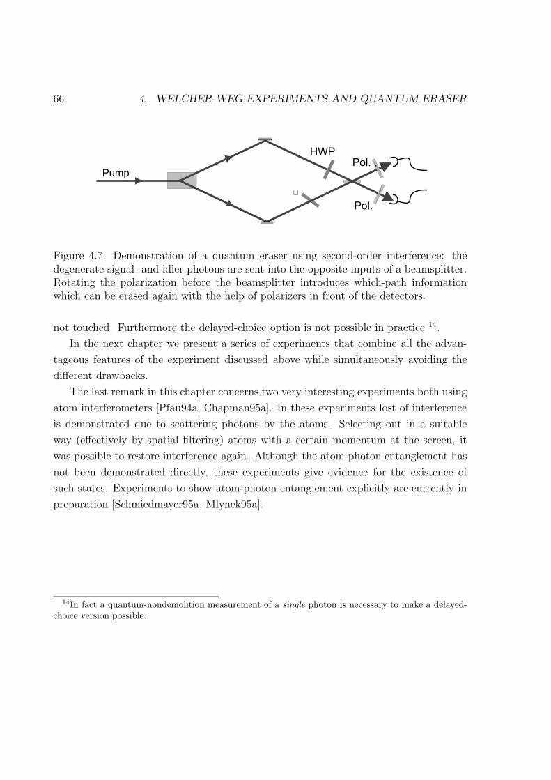
66 4. WELCHER-WEG EXPERIMENTS AND QUANTUM ERASER
'0!
!
Figure 4.7: Demonstration of a quantum eraser using second-order interference: thedegenerate signal- and idler photons are sent into the opposite inputs of a beamsplitter.Rotating the polarization before the beamsplitter introduces which-path informationwhich can be erased again with the help of polarizers in front of the detectors.
not touched. Furthermore the delayed-choice option is not possible in practice 14.
In the next chapter we present a series of experiments that combine all the advan-
tageous features of the experiment discussed above while simultaneously avoiding the
different drawbacks.
The last remark in this chapter concerns two very interesting experiments both using
atom interferometers [Pfau94a, Chapman95a]. In these experiments lost of interference
is demonstrated due to scattering photons by the atoms. Selecting out in a suitable
way (effectively by spatial filtering) atoms with a certain momentum at the screen, it
was possible to restore interference again. Although the atom-photon entanglement has
not been demonstrated directly, these experiments give evidence for the existence of
such states. Experiments to show atom-photon entanglement explicitly are currently in
preparation [Schmiedmayer95a, Mlynek95a].
14In fact a quantum-nondemolition measurement of a single photon is necessary to make a delayed-choice version possible.

“It has not yet become obvious to me thatthere’s no real problem, therefore I suspectthere’s no real problem, but I’m not surethere’s no real problem. So that’s why I liketo investigate things.”
Richard P. Feynman 1982
5 From Theory to Practice – The
Two-Photon Quantum Eraser
5.1 Introduction
We present various experiments demonstrating the mutual exclusivity of observing which-
path information and interference in a single experiment. Similar to the past experiments
discussed in the last chapter, we also employed the correlated photon pairs produced in
PDC. Different degrees of freedom, polarization and time, has been used to mark the
path of the interfering photon. In the first series of experiments we applied our quantum
marker directly to the interfering photon. In particular we paid some attention to the
case of incomplete which-path information and the case of a partial quantum eraser.
The former means that the paths were not made totally distinguishable whereas the
latter means that the which-path information was not completely erased.
However, as the main result, it turns out that no which-path measurements need to
be performed on the interfering photon itself. Instead one of the photons can be used
as the interfering system whereas the conjugate photon can be used as our quantum
system on which the path detection may be performed. In our experiments we produced
explicitly an entangled state of the interfering photon with the measurement-photon.
67

68 THE TWO-PHOTON QUANTUM ERASER
Using this entanglement perform either path-detection or realize the quantum eraser.
In this case our which-path detector can be viewed as spatially separated from the
interfering system. Moreover we think that our detection scheme does not entail any
momentum transfer to the interfering particle. Therefore coherence is lost only due to
complementarity.
At the end we describe a feasible extension of the experiment to demonstrate the
delayed choice aspect mentioned in the last chapter.
The described experiments demonstrate explicitly that a measurement need not be
irreversible as long as the result has not been recorded by a classical apparatus. In this
sense one can imagine experiments in which one can switch arbitrarily often between
which-path information and interference. Only the irreversible detection of the photon
establishes a complete measurement.
5.2 Experimental setup
The starting point for all experiments was the railcross-setup, discussed in detail in
chapter 3. Throughout the rest of this chapter we will refer for convenience to the
down-conversion photons created by a pump photon in its first (second) pass through
the crystal as being “reflected” (“direct”). The same wavelengths for signal and idler
were used (633nm and 789nm); the pump laser (351nm) had a typical power of about
100mW. At the very first let us remind for two important features. Firstly due to the
type-I phasematching condition governing the nonlinear process in LiIO3 all the signal-
and idler photons that are generated in the crystal are born with vertical polarization.
Secondly the absolute distance from the crystal to the mirrors is in principle not an
important parameter for the interference to occur. The experiment affords only that
the distances from the crystal to signal- and idler-mirror have to coincide within the
coherence length of the photons arriving at the corresponding detector. In other words
it is necessary that the detected photons are temporarily indistinguishable in principle.
Introducing explicitly time and polarization as degrees of freedom the two-photon state

THE TWO-PHOTON QUANTUM ERASER 69
as emitted by the down-conversion into the modes |〉i and |〉s can be written in the form:
|Ψ〉 = eiφp |V 〉s|V 〉i + ei(φs+φi)|V 〉s|V 〉i (5.1)
As shown in chapter 3 this state leads to first-order interference according to Is = Ii ∝12(1 + cos(∆φ)) = 1
2(1 + cos(φp − φs − Φi)).
The experimental arrangement affords easy access to the beam paths between the
crystal and the mirrors (these distances were about 13 cm in our experiment). Thus we
can manipulate the reflected downconversion photons in such a way that they become
distinguishable from those emitted directly to the detectors. We have two possible types
of a quantum marker implementable in the setup (see also Fig.5.1):
• Firstly we can manipulate the polarization of either of the reflected signal- and
idler modes.
• Secondly we can translate the signal- or idler-mirror by a distance that is larger
than the coherence length. Then it is in principle possible (although not in prac-
tice) to distinguish the origin of the photon by measuring the time difference.
In practice the polarization was turned with the help of a quarter wave plate (QWP)
placed in front of either the signal and idler mirror. Upon double passage this device
works effectively as a halfwave plate . The erasing of the polarization information was
accomplished by placing a polarizer in front of the signal detector. At the idler detector
we used a polarizing beamsplitter (PBS) in combination with a halfwave plate (HWP)
as analyzer. For convenience we will name the idler transmitted through the PBS idler-I
and the idler reflected at the PBS idler-II. With the various coincidences we will deal in
an analogous way.
In another series of experiments we employed various interference filter in front of
the detectors. Two different bandwidths were used, one with a FWHM of 5nm and one
with 0.5nm. In practice the spectral width of the downconverted light measured by the
detectors was limited in the case of the 5nm-filter to about 1.5nm because of the small
size of the irises (see also chapter 3.4).

70 THE TWO-PHOTON QUANTUM ERASER
10
10
!
!
!
%2!3
Figure 5.1: The principle experimental setup used for all quantum eraser experiments.The rather long distance from the crystal to the mirrors allows easy access to the modesbetween them. The quantum marker was realized either by turning the polarizationof the reflected photons or by shifting the signal or idler mirror outside the interfer-ence region. Erasing the which-path information was accomplished by using polarizingelements or interference filters before the detectors.
One should still note that because all the experiments described in the following deal
with polarization, one has to pay attention to the problem of double refraction within
the crystal. Rotating the polarization of the reflected photons results in a transversal
and a longitudinal displacement of the photons upon passage through the crystal with
respect to the direct vertical polarized photons. The longitudinal displacement can be
compensated easily by shifting one of the mirrors, but the transversal shift leads to
a separation of the modes and makes them distinguishable. Such a shift should be
minimized for that reason. To overcome this obstacle we employed a thin LiIO3-crystal
with a length of 1mm. The remaining transverse shift (beam walkoff) amounts to about
18µm for the signal and 25µm for the idler beam that can be tolerated. However for
the 3cm-crystal which we used in capter 3 the walkoff increases up to about 600µm.

THE TWO-PHOTON QUANTUM ERASER 71
5.3 Quantum marker and quantum eraser experi-
ments on single photons
5.3.1 Polarization as quantum marker
In the first series of experiments our quantum marker consisted of a quarterwave plate
polarization retarder in front of the mirror in the idler mode (Fig.5.2a). Correctly
oriented, this plate rotated the polarization from vertical (V) to horizontal (H) upon
double passage. The resulting state of the downconverted light can be written as
|Ψ〉 λ/4−−→ |V 〉s|V 〉i + ei∆φ|H〉s|V 〉i (5.2)
One now has the possibility1to obtain which-path information for the idler photon
just by measuring whether its polarization is H (a reflected idler) or V (a direct idler
photon). The mere existence of this possibility demands that there cannot be any
interference for the idler, because only processes that are indistinguishable in principle
can interfere. It also demands that there cannot be any interference for the signal photon
either, since the two photons are always created in pairs, and which-path information
for one photon necessarily implies which-path information for the other.
The left column in Fig.5.2 shows experimental results that demonstrate these ideas.
From top to bottom are plotted: the signal singles count rate, both idler count rates
and additionally the coincidences between signal and the transmitted idler (see also Fig.
5.2b)). The data were evaluated as discussed in chapter 3 by subtracting background
and fitting cosine functions. None of the curves displays any modulation (the remaining
interference visibility amounted typically to about 1%).
However, one may erase the which-path information carried by the idler photon
by measuring its polarization along +45 or −45 (Fig. 5.2a). This corresponds to a
measurement in a basis rotated by 45 compared with the H-V basis. Eq.(5.2) can be
1In practice the which-path measurement was realized by turning the HWP parallel to the H- orV-direction (see also above). The PBS allowed us to observe the orthognal polarizations simultaneously.

72 THE TWO-PHOTON QUANTUM ERASER
rewritten in this basis as follows:
|Ψ〉 Pol. BS
45−−→ 1√
2
((1 + ei∆φ)|+ 45〉i + (1− ei∆φ)| − 45〉i
)|V 〉s. (5.3)
It is then not possible, even in principle, to tell whether a idler registered after the
polarizer was initially H- or V- polarized, and consequently both idler count rates again
showed interference if any of the mirrors were moved (Fig. 5.2c). The interference in the
idler and also in the coincidences could be regained completely, that is we observed the
same visibility as for the normal “railcross”-experiment: about 57% in the transmitted
idler, 30% in the idler reflected at the PBS and 80%–90% in the coincidences. It is
worth mentioning that the fringes in both idler count rates were opposite in phase.
One can explain this easily by inspecting eq.(5.3). A photon transmitted through the
PBS corresponds to measuring the photon in state |45〉 whereas finding the photon in
the other output of the PBS corresponds to the state | − 45〉. The former leads to a
modulation with 1 + cos(∆φ), the latter to 1− cos(∆φ).
Note that the erasure of the idler photon’s path information had no influence on
the detection of the signal photon and does not suffice to restore interference in the
signal count rate. This could also be observed in the experiment. Loosely stated, the
signal photon could not “know” how the distant idler polarizer would be oriented2. One
should emphasize too, that the mere passage through a polarizing beam splitter does not
constitute a measurement of the polarization — one could always recombine the output
beams in another beam splitter to change the analysis basis such that one has access to
the path-information again. Only after an irreversible detection of the photon one may
speak of a measurement having performed.
As indicated in chapter 4, one should employ single particles for the interfering system
in order for the which-path notion to be meaningful. Conditioned upon detection of
the signal photon, the idler photon is prepared in a single-photon state [Grangier86a].
Therefore, the coincidence detection gave the result for which-path and quantum-eraser
measurements for the single idler photon (Fig. 5.2b,c), and we have fulfilled the basic
requirements for a Welcher-Weg and quantum eraser experiment explained in the last
2Otherwise one could use the experiment for superluminal communication.

THE TWO-PHOTON QUANTUM ERASER 73
Figure 5.2: a) Experimental setup demonstrating the use of a quantum marker (quarter-wave plate, QWP) to rotate the polarization from vertical () to horizontal (↔), anda quantum eraser (polarization analyzer). b) Signal- and both idler-count rates as wellas the coincidence count rate between signal and transmitted idler in the which-pathmeasurement (polarization analysis at 0). c) The corresponding rates for the quantumeraser experiment (polarization analysis at 45). (In practice the analysis was performedwith a polarizing beam splitter preceded by a rotatable half-wave plate.)

74 THE TWO-PHOTON QUANTUM ERASER
chapter. However the experiment lacked the additional ingredients discussed in the
last chapter. The which-path information was carried by the interfering particle itself.
It this sense there is no improvement over the past experiments (chapter 4). Strictly
speaking one should not name it a “quantum Eraser” at all because the same effect can
be observed on a classical level with classical fields (see also [Aschenwald93a]).
5.3.2 Time as quantum marker
In this section we show how one can use time as a degree of freedom to make two inter-
fering processes distinguishable. It is based on the following idea: the downconverted
photons are strongly correlated in time due to the energy conservation inherent in the
nonlinear process. The correlation time becomes non zero solely because of the finite
bandwidth of the detected photon i.e. the coherence time τc.
Therefore in our experiment, if we move for example the idler mirror by more than
a coherence length 6c = c/τc we mark the different paths again. We have now in
principle the possibility to determine the path by recording the detection times for each
photon accurately. If signal and idler photon hit the detector simultaneously (assuming
equal path lengths from the crystal to the detectors) we know for sure that they came
directly from the source. On the other hand if we measure a time difference the photons
werereflected at the mirrors. It is absolutely unimportant that a detector with such a
capability does not presently exist. The mere possibility is enough.
But again as long as the idler photon is not detected, this loss of interference is
reversible. However it turns out that it is more difficult to remove the distinguishability
in this situation because in contrast to the polarization experiment we cannot separate
the direct photons from the reflected photons after the crystal. Instead, similar as in
[Kwiat94e] one must use an extra interferometer in the idler beam in front of the detector
to mix both paths again (Fig.5.3a). The pathlengths of that interferometer must differ
by the same amount as the idler mirror has been moved. Now the photon pair has four
possibilities. One can easily see that only two of them are indistinguishable, the other
This method alone erases the which path information only partially. There are still
incoherent contributions for example if the idler photon goes the short way through

THE TWO-PHOTON QUANTUM ERASER 75
*4
5%
!
*4
Figure 5.3: a) A possible experiment adapted from [Kwiat94e]: The photons are labeledby shifting, for instance, the idler mirror more than a coherence length. Erasing ispartially accomplished by an interferometer in front of the idler detector. b) Our setupusing an narrow bandwidth interference filter
the interferometer and the signal photon goes via the mirror. To select out only the
indistinguishable contributions and to completely recover interference, it is additionally
necessary to make a very careful time measurement on the idler photon (e.g. by coinci-
dence detection with the signal photon) to exclude detection events which do not stem
from interfering photons.
In our experiment we used a simpler idea paying the price that we could only achieve
partial quantum erasing. By inserting a narrow bandwidth interference filter (0.5nm)
we increased the coherence length of the detected photons. Thus a possible timing mea-
surement can no longer resolve completely the origin of the photon pair and interference
is partially restored.
Fig.5.4 shows typical data. Actually we could measure both the which-path- and
the quantum eraser configuration at the same time. Because all polarizations were the
same (vertical) we could use the PBS to split the idler mode into two modes. These
were directed to separate detectors equipped with different interference filters. In one
of the output modes of the PBS we used a relative broad interference filter (effective
spectral width about 1.5nm corresponding to a coherence length of 280µm). The upper
plot depicts a coarse scan of this count rate that demonstrates the decrease in the
visibility of the interference pattern with increasing difference ∆x of the path lengths.
The inserts show two fine scans, one taken at the position ∆x = 0µm where maximal
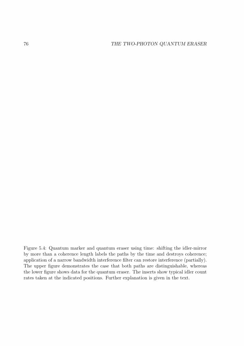
76 THE TWO-PHOTON QUANTUM ERASER
Figure 5.4: Quantum marker and quantum eraser using time: shifting the idler-mirrorby more than a coherence length labels the paths by the time and destroys coherence;application of a narrow bandwidth interference filter can restore interference (partially).The upper figure demonstrates the case that both paths are distinguishable, whereasthe lower figure shows data for the quantum eraser. The inserts show typical idler countrates taken at the indicated positions. Further explanation is given in the text.

THE TWO-PHOTON QUANTUM ERASER 77
interference (Vis≈ 27%) occurred, the other showing no modulation (Vis≈ 1%). The
latter was accomplished by shifting the mirror 400µm. Thus the real displacement was
2 × 400µm ≡ 800µm, which corresponds to about three times the coherence length.
Therefore which-path information was available in principle.
The lower part of the figure shows the count rate recorded in the other output of the
PBS. Here an interference filter with a bandwidth of about 0.5 nm was placed before
the detector resulting in a tripling of the coherence length. Consequently the fine scan
taken at the position ∆x = 400µm where the other count rate was already flat, exhibited
again fringes (Vis ≈ 20%). Note that due to the narrower interference filter, also the
visibility observed at ∆x = 0µm increased considerably to about 57%.
Again one may say that this experiment fulfilled the basic requirement of a which-
path and quantum eraser and again one may raise the same objections to it. Moreover
in this experiment the modes reflected from the interference filter were not really ac-
cessible in contrast to the polarization experiment. In this sense the interference filter
performs an irreversible measurement and we cannot undo its action again to regain
path information.
5.3.3 Effect of incomplete which-path information
Here we pay some attention to the problem of incomplete distinguishability of the paths.
For the polarization experiment we discussed only the two situations of perfect path-
information on the one hand and no path-information (optimal interference) on the other
hand. In this section we present an experimental study dealing with the intermediate
situation. Intuitively one expects that the visibility of the fringes will be neither perfect
nor zero. There should be a gradually transition from one extreme to the other. We
present quantitative data from both the polarization- and the time-arrangements which
show this behavior.
In the first series of experiments we turned the polarization of the reflected idler again
by 90 thereby obtaining maximal knowledge about the path. Now we gradually rotated
the polarization analyzer in front of the idler detector so that the output polarization

78 THE TWO-PHOTON QUANTUM ERASER
Figure 5.5: The left plot shows the dependence of the visibility on the analyzing angleof the polarization analyzer. The polarization of the reflected idler was turned by 90
to horizontal whereas the the reflected signal was left unchanged (vertical). In the rightplot additionally the polarization of the reflected signal was changed by 20.
varied from vertical (which-path) via 45 (interference) to horizintal polarization (which-
path) 3. We denote the angle of polarization under which we analyze the idler by θi.
Then the interference visibility of the idler count rate depends on θi as4
Vis(θi) = sin(2θi). (5.4)
For the coincidence rate one gets exactly the same dependence. The signal count rate
does not show any fringes at all. Note that the visibility becomes negative for θi > 90.
For this values of θi the fringes are shifted by 180 (see also Fig.5.2). The left plot of
Fig.5.5 shows the results. The curves agree quite good with the theory if one normalizes
each to the maximum visibility. The slightly different position of the maxima comes
3As earlier stated, this was performed by rotating the HWP in front of PBS from 0 via 22.5 to 454The derivation of all formulas in this section has been moved to appendix G. Nevertheless the reader
can understand the basic behavior without going into the mathematical details
THE TWO-PHOTON QUANTUM ERASER 79
from imperfect polarization components, particularly from the QWP.
What happens if one also turns the polarization of the signal? Obviously the in-
terfering paths idlers get an extra label because now one can look at the polarization
of the conjugate signal photon. Therefore one can expect that with increasing distin-
guishability of the signal paths the visibility in the idler count rate will decrease. The
theory predicts that one has to multiply all count rates with cos(φs) (φs is the amount
by that the signal polarization is turned). The right plot of Fig.5.5 shows that case. We
selected as an example φs = 20 with the expectation that the visibility decreases for
all count rates by a factor of 1− cos(20) = 0.934. The plotted data were also in good
agreement with this prediction although the change is difficult to see. If one turns the
the signal polarization by 90 interference disappears completely. Examples to prove
this will follow further below in section 5.4.(see Fig. 5.9).
Next we treated the case of incomplete distinguishability of the paths. That was done
by rotating the polarization of the reflected idler by an angle φi < 90. Intuitively one
may expect that interference should never vanish completely. But indeed it turns out
that it is still possible to perfectly determine the path of the photon. One can carry out
the measurement by turning the idler analyzer orthogonal to one of the polarizations. In
this case the photons detected behind the analyzer could arrive at the detector only via
one definite path. On the other hand in the middle between these two positions of the
polarizer (on both sides), perfect fringes can be obtained because for photons detected
in this case, both paths are equal probable. Quantitatively the visibility in the idler
count rate should have the following dependence on the analyzer angle θi:
Visi(θi) =2 cos(θi) cos(θi − φi)
cos2(θi) + cos2(θi − φi)(5.5)
The visibility in the signal does not show any dependence on θi (as expected). However
the visibility must be multiplied by the factor cos(φi) because the idler now carries a
certain amount of which-path information for the signal.
For the experiment we choosed φi = 30 (and φs = 0). Fig. 5.6 shows the result.
The data can be reproduced by the theory relativly good. Both positions of the zero
points (90 and 120) were exactly at the right analyzer orientations. The directions

80 THE TWO-PHOTON QUANTUM ERASER
Figure 5.6: In this experiment the polarization of the reflected idler was turned by 30
with respect to the vertical direction. The left column shows the visibilities of all singlecount rates in dependence θi, the right column the visibilities of all coincidences.

THE TWO-PHOTON QUANTUM ERASER 81
where maximal interference occurs were also in agreement with the theory. In particular
the idler- and coincidence count rates corresponding to the idler transmitted through
PBS (narrow bandwidth filter) agreed very well with the theory. Also the signal count
rate (top left) shows a visibility reduced by the right amount of 1 − cos(30) = 0.14
(From about 50% to 42%). The data for the idler-II and the coincidence-II count rates
show some deviations from the theoretical curve5. This discrepancy probably comes
most from imperfections of the QWP, the HWP and the PBS.
Figure 5.7: Effect of gradually increasing the path length difference between signal andidler. Each data point corresponds to a fine scan taken at this mirror position.
Finally we performed another study in which we gradually translated the idler mir-
ror thereby increasing the time information and decreasing the visibility. We show in
appendix E that the visibility in dependence on ∆x is given by the Fourier transform of
5Both the idler- and the coincidence count rates show the same behavior. These curves are shiftedby 90 with respect to the transmitted idler and coincidences because here we analyze in a basis turnedby 90
82 THE TWO-PHOTON QUANTUM ERASER
the spectral distribution function η2(ω) of the photons hitting the detector6:
Visi/s(∆x) =∫
dω|ηs/i(ω)|2eiω∆xc (5.6)
VisC(∆x) =∫
dω|ηi(ω)|2|ηs(ω)|2eiω∆xc (5.7)
With |ηs/i(ωs/i)|2 ∝ e−4 ln 2
(ωs0/i0−ωs/i)2
∆ω2s/i the FWHM-value of the visibility-functions are:
∆(∆x) =
2 ln 4π
λ2s/i
∆λs/ifor the singles
2 ln 4π
∆λ2sλ
4i+∆λ2
iλ4s
∆λs∆λifor the coincidences
(5.8)
Note that the visibility of the coincidences is determined by both the signal and idler
bandwidth with the result that the visibility decreases slower than for the singles.
Fig.5.7 shows for each single- and coincidence-count rate the visibility in dependence
on the mirror position. Each data point represents a fine scan taken at the corre-
sponding point. These data sets were fitted by a Gaussian function. This procedure
provided quantitative information about the bandwidth of the detected light (given by
the FWHM-value).
In the signal and the idler-I mode we used interference filter with a bandwidth of
0.5nm and 0.8nm. The bandwidth of the idler-II was effectively given by the irises and
had a value of about 1.6nm. Using these numbers we could calculate the widths of the
visibility functions and could compare it with the experimental results of the fits in Fig.
5.7. The following table shows he results. The agreement is quite well with the exception
of the coincidence count rate between signal and idler-II.
6According to our definition in chapter 3 gives |η(ω)|2 the spectral probability distribution to detecta photon behind the filter. The bandwidth of the filter is related to this function. η(ω) itself gives thefield distribution

THE TWO-PHOTON QUANTUM ERASER 83
calculated value measured value
Signal (0.5nm) 707µm 698µm± 20µm
Idler-I (0.8nm) 686µm 677µm± 22µm
Idler-II (1.6nm) 343µm 338µm± 15µm
Coinc. Signal-Idler-I 969µm 1017µm± 228µm
Coinc. Signal-Idler-II 772µm 645µm± 55µm
5.4 The two-photon quantum eraser
The main purpose of the experiments discussed in the last section was to demonstrate
some methods to label the paths of an interfering system and to subsequently erase this
labeling again. On the one hand all these experiments fulfilled the basic requirements
of a quantum eraser: we had an interfering system, a method to distinguish both paths
and we could erase this distinguishability again to restore interference.
However, strictly speaking one should not use the word quantum eraser in this context
without making some comments. Perhaps the most important disadvantage of these
experiments was the fact that the interfering system itself carried the path information.
The which-path detection process and the resulting nonseparability become much more
apparent when a system spatially distinct from the initial interfering system carries the
which-path information. As mentioned in chapter 5, it would be desirable if a separated
system would be used as label and if the the original system remains undisturbed. Here
however the state of this particle was changed explicitly. Moreover there would be no
difference in the result if we would use a classical light field (like a laser) instead of the
downconversion source [Aschenwald93a]. In the following we present two experiments
in which we avoided these problems.
The experiment described now starts from the polarization-experiment discussed in
the last section. We changed the setup in the sense that we rotated the polarization of
the reflected signal-photons by 90 instead of the reflected idler-photons. Consequently
a polarizer at 45 in front of the signal detector had to be used to restore first-order
interference again. That was done so that we would not have to rebuild the whole
experiment. It is advantageous to have access to both polarization components as we
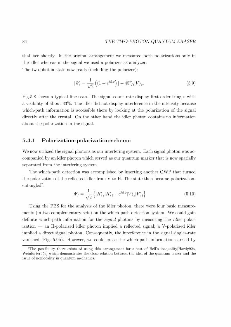
84 THE TWO-PHOTON QUANTUM ERASER
shall see shortly. In the original arrangement we measured both polarizations only in
the idler whereas in the signal we used a polarizer as analyzer.
The two-photon state now reads (including the polarizer):
|Ψ〉 = 1√2
((1 + ei∆φ
)|+ 45〉i|V 〉s. (5.9)
Fig.5.8 shows a typical fine scan. The signal count rate display first-order fringes with
a visibility of about 33%. The idler did not display interference in the intensity because
which-path information is accessible there by looking at the polarization of the signal
directly after the crystal. On the other hand the idler photon contains no information
about the polarization in the signal.
5.4.1 Polarization-polarization-scheme
We now utilized the signal photons as our interfering system. Each signal photon was ac-
companied by an idler photon which served as our quantum marker that is now spatially
separated from the interfering system.
The which-path detection was accomplished by inserting another QWP that turned
the polarization of the reflected idler from V to H. The state then became polarization-
entangled7:
|Ψ〉 = 1√2
|H〉s|H〉i + ei∆φ|V 〉s|V 〉i
(5.10)
Using the PBS for the analysis of the idler photon, there were four basic measure-
ments (in two complementary sets) on the which-path detection system. We could gain
definite which-path information for the signal photons by measuring the idler polar-
ization — an H-polarized idler photon implied a reflected signal; a V-polarized idler
implied a direct signal photon. Consequently, the interference in the signal singles-rate
vanished (Fig. 5.9b). However, we could erase the which-path information carried by
7The possibility there exists of using this arrangement for a test of Bell’s inequality[Hardy92a,Weinfurter95a] which demonstrates the close relation between the idea of the quantum eraser and theissue of nonlocality in quantum mechanics.
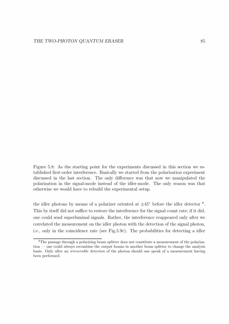
THE TWO-PHOTON QUANTUM ERASER 85
Figure 5.8: As the starting point for the experiments discussed in this section we es-tablished first-order interference. Basically we started from the polarization experimentdiscussed in the last section. The only difference was that now we manipulated thepolarization in the signal-mode instead of the idler-mode. The only reason was thatotherwise we would have to rebuild the experimental setup.
the idler photons by means of a polarizer oriented at ±45 before the idler detector 8.
This by itself did not suffice to restore the interference for the signal count rate; if it did,
one could send superluminal signals. Rather, the interference reappeared only after we
correlated the measurement on the idler photon with the detection of the signal photon,
i.e., only in the coincidence rate (see Fig.5.9c). The probabilities for detecting a idler
8The passage through a polarizing beam splitter does not constitute a measurement of the polariza-tion — one could always recombine the output beams in another beam splitter to change the analysisbasis. Only after an irreversible detection of the photon should one speak of a measurement havingbeen performed.

86 THE TWO-PHOTON QUANTUM ERASER
photon in coincidence with the signal photon (after its 45-polarizer) show opposite in-
terference oscillations for the two different idler polarizations [I(i+45) ∝ 1 + cos(∆φ);
I(i−45) ∝ 1− cos(∆φ)] (Fig. 5.9c). Note, the sum of these fringes and anti-fringes did
not display interference.
5.4.2 Polarization-time-scheme
In our final experiment we started with the same quarter-wave plate and 45-polarizer
arrangement in the idler beam as before, so that interference was observable in the idler
singles rate. However, we employed a different degree of freedom for labeling the signal
photon. By increasing the distance between the signal mirror and the down-conversion
crystal by more than the coherence length of the detected photons (6c ≈ 260µm), we
introduced the possibility to extract which-path information by measuring the relative
arrival times of the photons (Fig.5.10a). Fig.5.10b shows a coarse scan of the signal
mirror. Away from the ideal alignment (∆ = 0) the interference in the idler, apparent
in the large scatter of the intensity, rapidly faded away due to the in-principle temporal
distinguishability. The interference disappeared even though our detectors in practice
could not resolve these short time differences.
In this experiment, the erasure was accomplished by placing an interference filter with
a smaller bandwidth (0.5 nm FWHM) in front of the signal detector, thus increasing
the coherence length of the detected signal photons (6c ≈ 800µm) [Kwiat91a]. Since
the resulting coherence length was then greater than the relative delay (∆ = 425µm),
interference (with a lower visibility) was again observed after correlating the detection
of the idler photons with the registered signal photons, i.e., in the coincidence intensity
(Fig.5.10c).

THE TWO-PHOTON QUANTUM ERASER 87
Figure 5.9: a) Polarization of the idler photon is used as a quantum marker to distinguishthe signal photons. b) Which-path configuration: Neither of the singles and coincidencecount rates displays interference. c) Quantum eraser: using polarizers at 45
is not enough to regain interference in the single count rates. Correlation of the signalphotons with the detection of the idler photon restores the interference.

88 THE TWO-PHOTON QUANTUM ERASER
Figure 5.10: a)Experiment employing time delay as a quantum marker, and a narrow-bandwidth interferencefilter (IF) as the quantum eraser. b)Coarse scan of the sig-nal mirror, showing the loss of interference for the idler photons at large ∆. Thenarrow-bandwidth filter in the signal beam preserves interference in the coincidencerate. c)Phase scan for ∆ = 425µm.
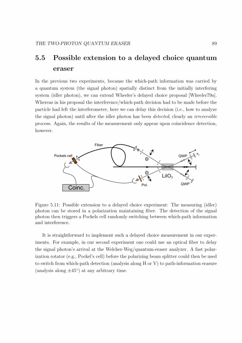
THE TWO-PHOTON QUANTUM ERASER 89
5.5 Possible extension to a delayed choice quantum
eraser
In the previous two experiments, because the which-path information was carried by
a quantum system (the signal photon) spatially distinct from the initially interfering
system (idler photon), we can extend Wheeler’s delayed choice proposal [Wheeler79a].
Whereas in his proposal the interference/which-path decision had to be made before the
particle had left the interferometer, here we can delay this decision (i.e., how to analyze
the signal photon) until after the idler photon has been detected, clearly an irreversible
process. Again, the results of the measurement only appear upon coincidence detection,
however.
!
%-
/
Φ10
10!
Figure 5.11: Possible extension to a delayed choice experiment: The measuring (idler)photon can be stored in a polarization maintaining fiber. The detection of the signalphoton then triggers a Pockels cell randomly switching between which-path informationand interference.
It is straightforward to implement such a delayed choice measurement in our exper-
iments. For example, in our second experiment one could use an optical fiber to delay
the signal photon’s arrival at the Welcher-Weg/quantum-eraser analyzer. A fast polar-
ization rotator (e.g., Pockel’s cell) before the polarizing beam splitter could then be used
to switch from which-path detection (analysis along H or V) to path-information erasure
(analysis along ±45) at any arbitrary time.
90 THE TWO-PHOTON QUANTUM ERASER
5.6 Conclusion
In the experiments presented here, we used photon pairs together with different types of
quantum markers to perform which-path and quantum eraser operations. Note that our
markers and erasers allowed continuous variation of the degree of obtainable Welcher-
Weg information, thus causing a continuous loss of interference, in agreement with Bohr’s
complementarity principle. Note further that the which-path detection and quantum
erasing were carried out on a system spatially separated from the interfering system.
The use of mutually exclusive settings of the experimental apparatus implies the
complementarity between complete path information and the occurrence of interference.
In conclusion, our results corroborate Bohr’s view that the whole experimental setup
determines the possible experimental predictions.

“A vacuum is a hell of a lot better than someof the stuff that nature replaces it with”
Tennessee Williams
6 Can One detect Virtual Photons?
6.1 Introduction
In this final chapter we come back to the original “railcross”-experiment of chapter 3.
However this time we want to throw light upon it from a different point of view. As
already mentioned at the beginning of chapter 3, it is possible to apply some ideas of
cavity-quantum electrodynamics (cavity-QED) to thios measurements. Experimentally
this approach is supported by the observation that both the signal- and idler-count rates
go up and down with the same phase upon variation of a mirror position. Therefore it is
allowed to describe a minimum in terms of suppression of the emission into these partic-
ular modes whereas, in the opposite case of a maximum, one may speak of enhancement
of the emission.
This results suggest a comparison of the experimental results with some experiments
concerning an atom near a conducting surface (e.g. a mirror). The modification of the
spontaneous emission rate observed in the atomic system, is usually explained as due to
a change of coupling of the atom to the vacuum by the surrounding mirrors causing an
increase or decrease of the decay rate. Here on the other hand we propose a different
interpretation of inhibited (enhanced) spontaneous emission as caused by destructive
(constructive) interference of different possibilities for the photon to be emitted. In
this picture the emission probability itself remains unchanged no matter whether there
is a mirror or not. Only interference is responsible for the observed modifications of
the spontaneous emission rate. We discuss experiments that are based on the railcross
91
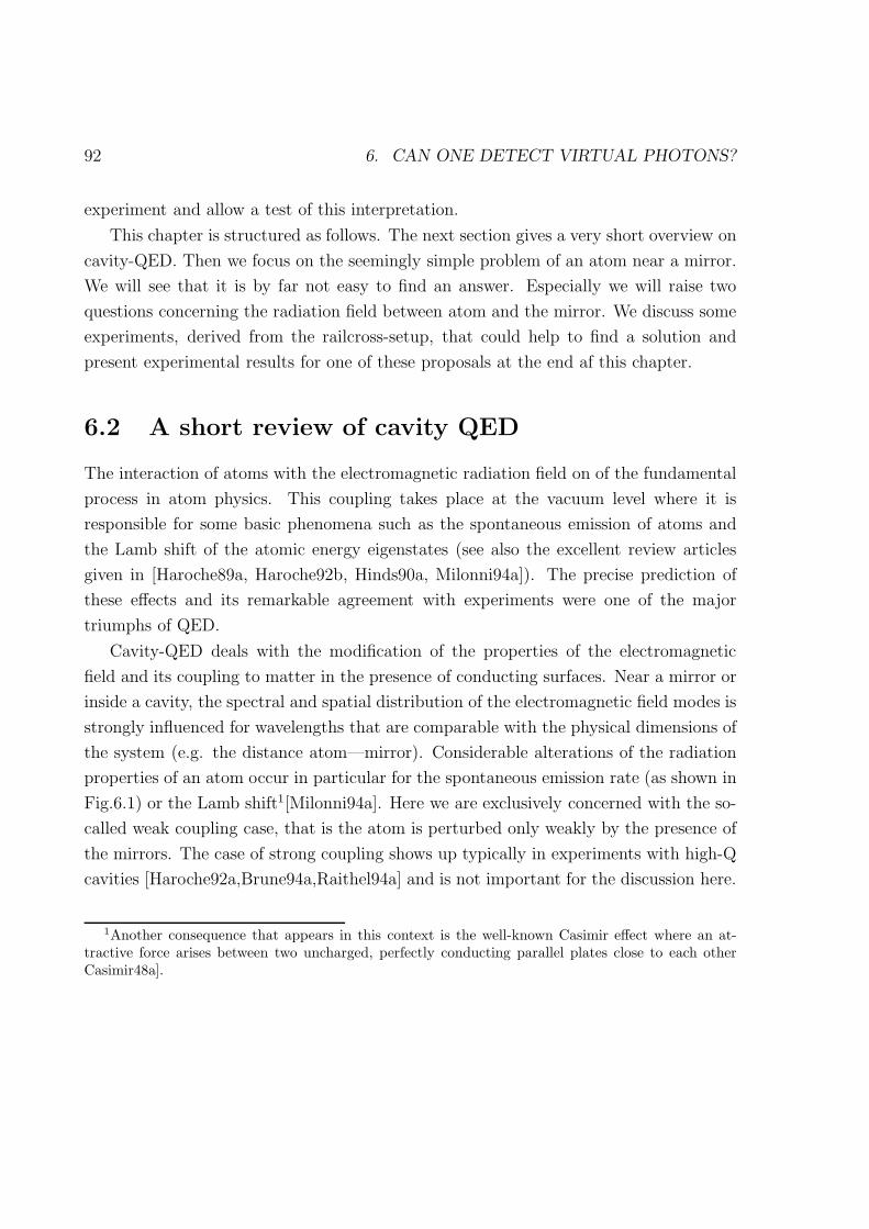
92 6. CAN ONE DETECT VIRTUAL PHOTONS?
experiment and allow a test of this interpretation.
This chapter is structured as follows. The next section gives a very short overview on
cavity-QED. Then we focus on the seemingly simple problem of an atom near a mirror.
We will see that it is by far not easy to find an answer. Especially we will raise two
questions concerning the radiation field between atom and the mirror. We discuss some
experiments, derived from the railcross-setup, that could help to find a solution and
present experimental results for one of these proposals at the end af this chapter.
6.2 A short review of cavity QED
The interaction of atoms with the electromagnetic radiation field on of the fundamental
process in atom physics. This coupling takes place at the vacuum level where it is
responsible for some basic phenomena such as the spontaneous emission of atoms and
the Lamb shift of the atomic energy eigenstates (see also the excellent review articles
given in [Haroche89a, Haroche92b, Hinds90a, Milonni94a]). The precise prediction of
these effects and its remarkable agreement with experiments were one of the major
triumphs of QED.
Cavity-QED deals with the modification of the properties of the electromagnetic
field and its coupling to matter in the presence of conducting surfaces. Near a mirror or
inside a cavity, the spectral and spatial distribution of the electromagnetic field modes is
strongly influenced for wavelengths that are comparable with the physical dimensions of
the system (e.g. the distance atom—mirror). Considerable alterations of the radiation
properties of an atom occur in particular for the spontaneous emission rate (as shown in
Fig.6.1) or the Lamb shift1[Milonni94a]. Here we are exclusively concerned with the so-
called weak coupling case, that is the atom is perturbed only weakly by the presence of
the mirrors. The case of strong coupling shows up typically in experiments with high-Q
cavities [Haroche92a,Brune94a,Raithel94a] and is not important for the discussion here.
1Another consequence that appears in this context is the well-known Casimir effect where an at-tractive force arises between two uncharged, perfectly conducting parallel plates close to each otherCasimir48a].

6. CAN ONE DETECT VIRTUAL PHOTONS? 93
Figure 6.1: Modification of the radiative decay rate in presence of a mirror in dependenceon the atom–mirror spacing: a) atomic dipole parallel to the mirror; b) atomic dipolenormal to the mirror (taken from??)
Modification of the spontaneous emission of an atom by its surrounding environment
was first suggested by [Purcell46a]. Recently the phenomenon has been investigated in
various elegant experiments involving atoms close to mirrors [Drexhage74a, Deppe90a].
They studied the fluorescence of optically excited organic-dye molecules that were sep-
arated from a metallic surface by a dielectric layer of known thickness, which resulted
in alterations of both the lifetime and of the angular distribution of the fluorescence.
Modification of atomic decay rates within cavities has been demonstrated for the
first time by [Goy83a]. Sodium atoms excited to Rydberg states were sent through high
finesse microwave cavities. On resonance enhancement of spontaneous decay by a factor
of 500 compared with the free space emission rate could be observed. On the other
hand the free-space rate was so slow that inhibition of spontaneous emission could not
be detected in the nonresonant case. This could be improved considerably [Hulet85a]
by sending a beam of Cs-atoms that were also excited up to Rydberg states through
a wave guide structure whose cutoff frequency was higher than the atomic transition
frequency. An increase of the spontaneous lifetime by a factor of about 20 could be
94 6. CAN ONE DETECT VIRTUAL PHOTONS?
observed. The experiments could be extended to the optical domain by using a smaller
wave guide in [Jhe87a]. Analoguos experiments were suggested in three-dimensional
dielectric media[Yablonovitch87a].
The experiments discussed so far were performed on setups involving very small
atom-mirror spacings of the order of a few wavelengths. But there were also experi-
ments involving cavities whose dimensions were much larger than the radiation wave-
length. One example by [Gabrielse85a] was the observation that single electrons in a
Penning trap could survive in excited states of the cyclotron motion for longer than
the natural lifetime due to the cavity structure of the electrodes. A different example
involving macroscopic cavities was described in [Heinzen87a]. They measured the visible
fluorescence of Ytterbium-atoms that were excited near the center of a confocal cavity.
The mirrors of the cavity were spaced 5cm apart, the finesse was about 70 that is by
far not an impressive value. However suppression by a factor of 42 of the spontaneous
emission into the cavity modes could be observed. In that case the confocality of the
resonator effects that a large number of spatial modes in the cavity are degenerate in
the frequency. The spontaneous decay into all these modes is modified in the same way.
6.3 An atom and a mirror - two possible interpreta-
tions
Now we restrict ourself to the seemingly simple case of an atom nearby a mirror. We sim-
plify the problem to the one-dimensional case (see Fig. 6.2). That means the atom can
only emit towards the detector or in the opposite direction. In the usual picture the al-
teration of spontaneous emission is explained as a consequence of the modification of the
vacuum field that couples to the atom. Sometimes one introduces the notion of “virtual
photons” that are exchanged between atom and mirror [Cook87a, Cohen-Tannoudji92a].
Here we want to offer an alternative interpretation of this phenomenon. In a simple
description light propagating from an atom placed close to a mirror can reach a detector
either directly or via reflection in the mirror. When the two paths cannot be distin-
guished, constructive and destructive interference effects occur between the probability
6. CAN ONE DETECT VIRTUAL PHOTONS? 95
amplitudes of both emission processes. When the atom-mirror distance is sufficiently
small, i.e. of the order of the wavelength, emission towards the detector can be sup-
pressed or enhanced depending on the distance of the atom from the mirror. Now we
interpret the modification of spontaneous emission to be due to destructive resp. con-
structive interference between the two possibilities of the photon to reach the detector.
The critical distance here is given by the coherence length of the emitted radiation. For
larger distances, interference can no longer occur. Consequently one should not observe
changes in the emission rate towards the detector. In fact we have already mentioned
above that the overall spontaneous emission only shows clearly pronounced effects if the
atom stays very close to the mirror, i.e. within distances of the order of a wavelength
(see also Fig. 6.1). For larger distances a modifcation is obscured by the possibility of
the atom into all the other modes which are affected by the mirror only for very small
distances.
One may ask which of the interpretations is correct. We will put this question
differently. Assume we adjust the experiment such that the spontaneous emission is
suppressed completely. In this case what is the state of the field between the atom
and the mirror? A (perhaps naive) look at the first interpretation suggests that there
should be just the vacuum field and nothing else. That means when replacing the
mirror by a detector, it should not be possible to see a photon instantaneously. Only
after a time T = dc(d: distance atom–mirror; c: speed of light) that is needed to
propagate the information about the removal of the mirror, the atom should start to
radiate and only after the time 2T the detector should start firing. On the other hand
it follows from the second picture that there is always a probability to find the photon
there because the probability amplitudes for the atom to emit the photon either via the
mirror or directly towards the detector are nonvanishing. Only the superposition of both
amplitudes as seen by the observer interferes destructively. In this sense the state of the
combined system (atom–field between atom and mirror) is entangled. Either the atom
is in the excited state and no photon is in the field or the the atom is in the ground state
and the field contains one photon. Therefore, in this picture, the can register photons
immediately after replacing the mirror.
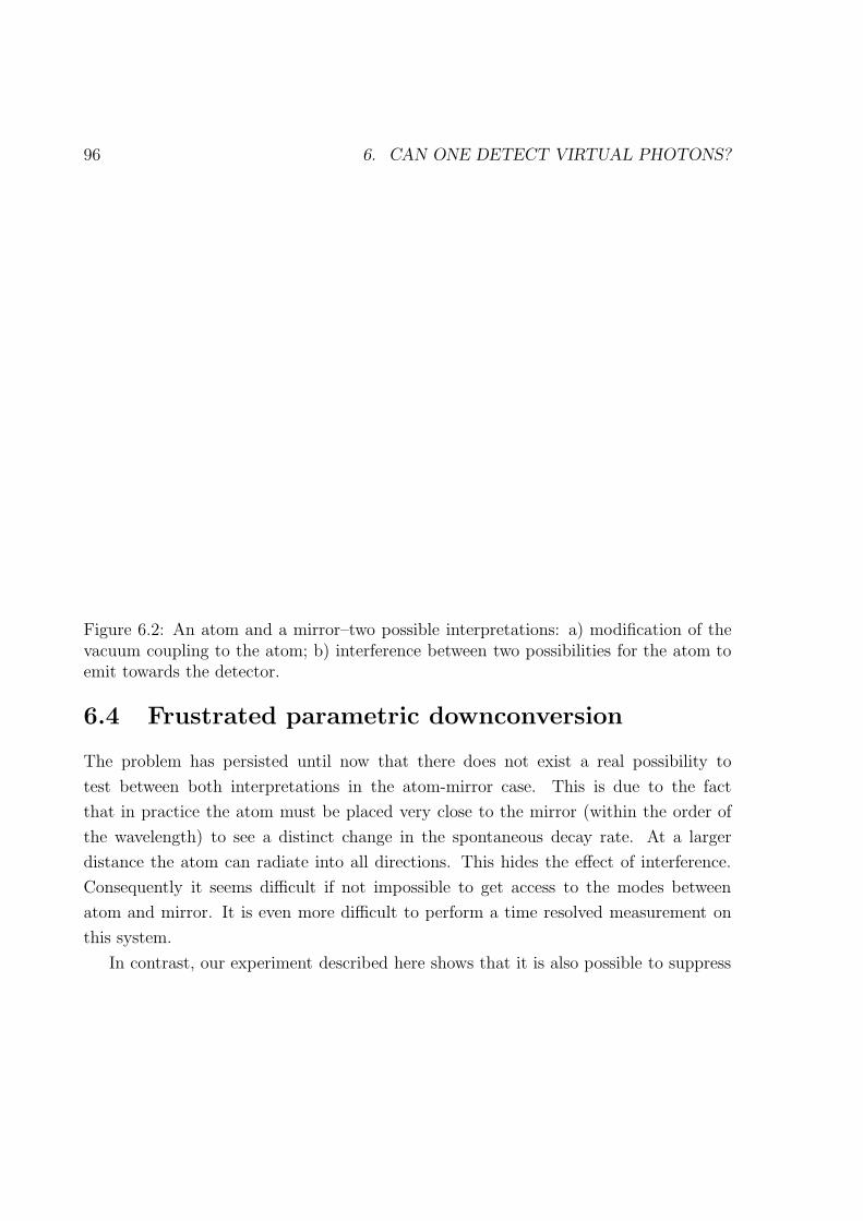
96 6. CAN ONE DETECT VIRTUAL PHOTONS?
Figure 6.2: An atom and a mirror–two possible interpretations: a) modification of thevacuum coupling to the atom; b) interference between two possibilities for the atom toemit towards the detector.
6.4 Frustrated parametric downconversion
The problem has persisted until now that there does not exist a real possibility to
test between both interpretations in the atom-mirror case. This is due to the fact
that in practice the atom must be placed very close to the mirror (within the order of
the wavelength) to see a distinct change in the spontaneous decay rate. At a larger
distance the atom can radiate into all directions. This hides the effect of interference.
Consequently it seems difficult if not impossible to get access to the modes between
atom and mirror. It is even more difficult to perform a time resolved measurement on
this system.
In contrast, our experiment described here shows that it is also possible to suppress

6. CAN ONE DETECT VIRTUAL PHOTONS? 97
or enhance the PDC into a specific pair of spatial modes for very large crystal to mirror
distances. The above mentioned problem can be overcome because of the very high
photon flux in the pump beam, which leads to a quite high emission rate in any spatial
direction. In principle the mirrors can be placed arbitrarily far away, only the relative
distances are restricted by the various coherence lengths (see also chapter 3). Similar
to the quantum eraser experiments discussed in the last chapter we have relatively easy
access to the mode between crystal and mirror. Loosely speaking we replace the atom
by a pump photon, the spontaneous emission occurs if the pump photon decays into a
signal and a idler photon (similar to a two-photon decay of an atom). In the following
we propose possible experiments that may allow to test the question we have addressed
in the last section. Furthermore we discuss how far they can be extended to the “atom–
mirror” case.
What do we expect to see in the case of frustrated parametric downconversion? Fol-
lowing the first argument given above we may describe the PDC as caused by the vacuum
field that mixes with the pump beam within the nonlinear crystal. If the radiating part
of the crystal is located at a node of the field, emission is suppressed. In this picture one
would expect that the crystal cannot radiate into the modes between the crystal and
mirror. Therefore instantaneously replacing one of the mirror by a detector, photons
would not be detected before a time delay of T = 2dc.
In contradiction to this statement we now describe a model that would predict no time
delay between insertion of the detector and detection of photons. In this model we treat
the downconversion process similar to a usual beamsplitter with very low reflectivity
corresponding to the low probability of the PDC-process. In this sense the description is
formally analogous to one of a Michelson interferometer. Note that this model assumes
equal amplitude α for upconversion and for downconversion2. |p〉 is the initial state of
the pump which we assume to br a single mode coherent state. Then the effect of PDC
2Talking about upconversion we mean spontaneous upconversion of a signal-idler photon pair to apump photon. As shown already at the end of chapter 3, upconversion stimulated by photon pairscreated in the first process is negligible here.

98 6. CAN ONE DETECT VIRTUAL PHOTONS?
can be described as follows (for the notation see chapter 3):
|Ψ〉 =√1− |α|2|p〉+ α|s1〉|i1〉 (6.1)
Reflecting the pump back through the crystal gives another possibility for downconver-
sion and it follows for the state:
|Ψ〉 = α (|s1〉|i1〉) +√1− |α|2eiφp
(√1− |α|2|p〉+ α|s2〉|i2〉
)(6.2)
Finally we reflect also the signal and idler beams originating in the first process back
into the crystal (with phase shifts φs and φi). Again we set |〉s1→ |〉s2
=: |〉s and
|〉i1 → |〉i2 =: |〉i. Including the possibility of upconversion of the first signal-idler pair
to a pump photon we now obtain:
|Ψ〉 = αei(φs+φi)(√
1− |α|2|s〉|i〉+ α|p〉)
+√1− |α|2
(√1− |α|2|p〉+ α|s〉|i〉
)
=√1− |α|2α
(ei(φs+φi)+eiφp
)|s〉|i〉
+[(1− |α|2)eiφp − |α|2ei(φs+φi)
]|p〉 (6.3)
For the intensities it follows:
Is = Ii ∝ A[1 + cos(φs + φi − φp)
](6.4)
Ip ∝ 1−A[1 + cos(φs + φi − φp)
](6.5)
with A = 2|α|2(1− |α|2)
The signal and idler intensity behave the same as before, but now the intensity of
the reflected pump beam depends also on the phase settings within the interferometer
although with the opposite phase. That means destructive interference between the
downconverted photons occurs at the same time with constructive interference between
the amplitude of the reflected pump and the amplitude of the upconversion process.
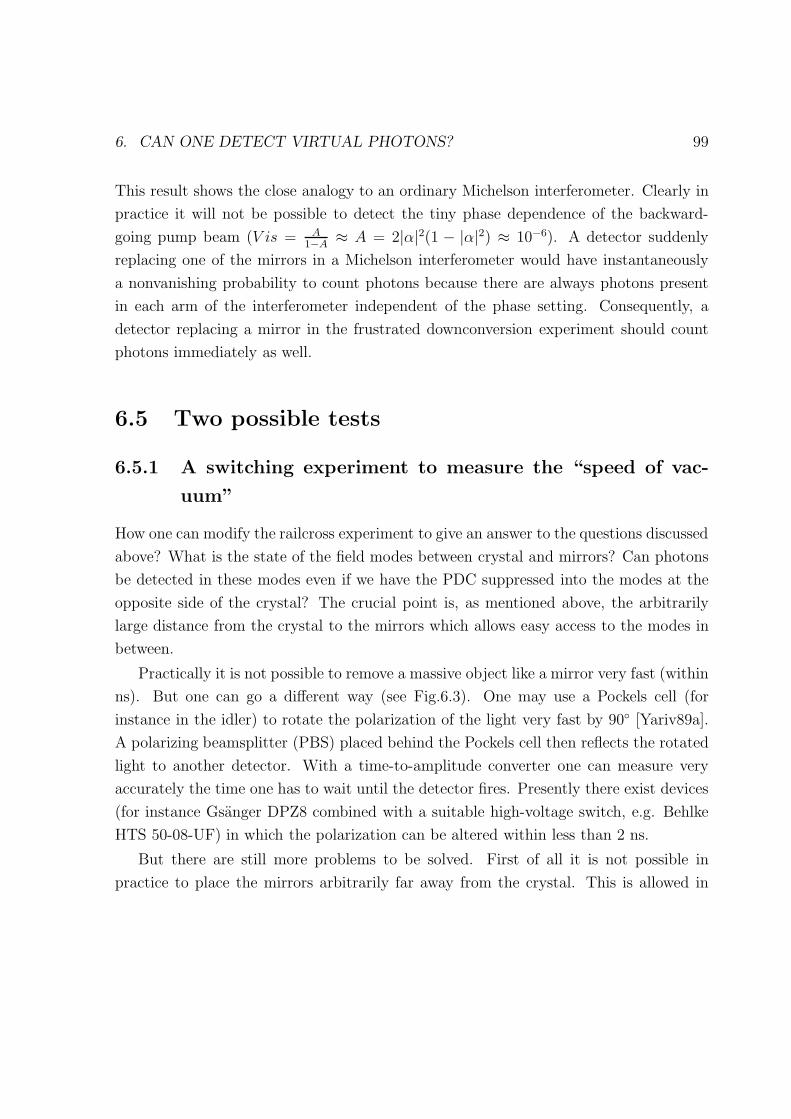
6. CAN ONE DETECT VIRTUAL PHOTONS? 99
This result shows the close analogy to an ordinary Michelson interferometer. Clearly in
practice it will not be possible to detect the tiny phase dependence of the backward-
going pump beam (V is = A1−A ≈ A = 2|α|2(1 − |α|2) ≈ 10−6). A detector suddenly
replacing one of the mirrors in a Michelson interferometer would have instantaneously
a nonvanishing probability to count photons because there are always photons present
in each arm of the interferometer independent of the phase setting. Consequently, a
detector replacing a mirror in the frustrated downconversion experiment should count
photons immediately as well.
6.5 Two possible tests
6.5.1 A switching experiment to measure the “speed of vac-
uum”
How one can modify the railcross experiment to give an answer to the questions discussed
above? What is the state of the field modes between crystal and mirrors? Can photons
be detected in these modes even if we have the PDC suppressed into the modes at the
opposite side of the crystal? The crucial point is, as mentioned above, the arbitrarily
large distance from the crystal to the mirrors which allows easy access to the modes in
between.
Practically it is not possible to remove a massive object like a mirror very fast (within
ns). But one can go a different way (see Fig.6.3). One may use a Pockels cell (for
instance in the idler) to rotate the polarization of the light very fast by 90 [Yariv89a].
A polarizing beamsplitter (PBS) placed behind the Pockels cell then reflects the rotated
light to another detector. With a time-to-amplitude converter one can measure very
accurately the time one has to wait until the detector fires. Presently there exist devices
(for instance Gsanger DPZ8 combined with a suitable high-voltage switch, e.g. Behlke
HTS 50-08-UF) in which the polarization can be altered within less than 2 ns.
But there are still more problems to be solved. First of all it is not possible in
practice to place the mirrors arbitrarily far away from the crystal. This is allowed in

100 6. CAN ONE DETECT VIRTUAL PHOTONS?
!
.
Figure 6.3: An possible experiment to measure the speed of vacuum: The combinationPockels cell–polarizing beamsplitter (PBS) allows us to quickliy switch a detector intothe idler mode between crystal and mirror. Using such a device one can measure inprinciple how much time it takes the crystal starts to radiate.
principle only for the case of infinite, plane modes. In reality we have to deal with
curved, divergent modes. If the mirrors are too far away, the mode mismatch between
the direct light and the light reflected at the mirrors increases. This results in a fringe
pattern that can no longer be resolved by the detector. In the current experimental
setup, the mirrors were placed about 13cm from the crystal. At this distance there is
not enough room for a Pockels cell and PBS. Possibly the use of spatial filters in the
pump beam and in front of the various detectors could help to move the mirrors farther
away3.
The mean single count rate that one can expect for the detector is on the order of
1000 per sec. However only the photons counted in the first ns (i.e. within the delay
time) are significant. The maximum switching rate of the high voltage switch is for
short times (a few seconds) of the order of 1 MHz. This means one may expect one
3We tried spatial filters as mentioned in chapter 3. However we found it very difficult to align thesetup and the typical count rates decreased by an intolerable amout
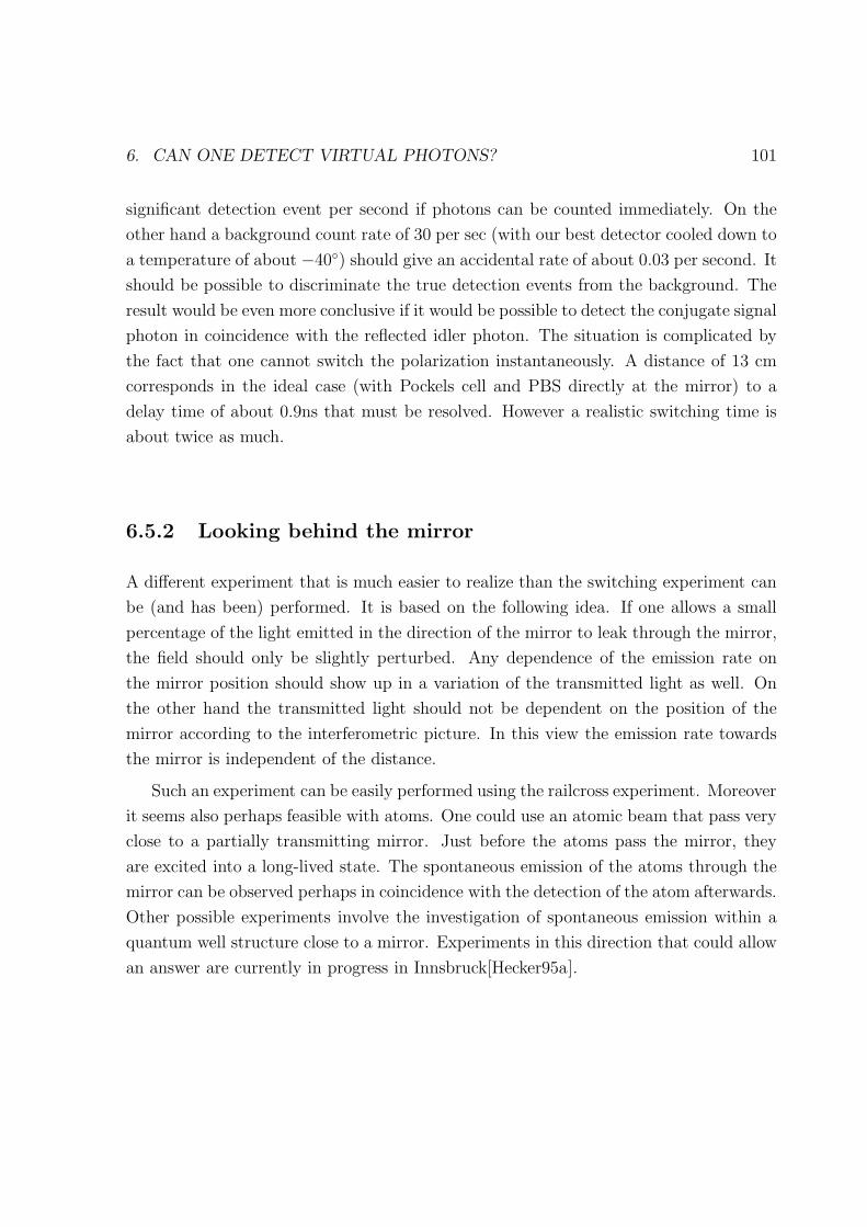
6. CAN ONE DETECT VIRTUAL PHOTONS? 101
significant detection event per second if photons can be counted immediately. On the
other hand a background count rate of 30 per sec (with our best detector cooled down to
a temperature of about −40) should give an accidental rate of about 0.03 per second. It
should be possible to discriminate the true detection events from the background. The
result would be even more conclusive if it would be possible to detect the conjugate signal
photon in coincidence with the reflected idler photon. The situation is complicated by
the fact that one cannot switch the polarization instantaneously. A distance of 13 cm
corresponds in the ideal case (with Pockels cell and PBS directly at the mirror) to a
delay time of about 0.9ns that must be resolved. However a realistic switching time is
about twice as much.
6.5.2 Looking behind the mirror
A different experiment that is much easier to realize than the switching experiment can
be (and has been) performed. It is based on the following idea. If one allows a small
percentage of the light emitted in the direction of the mirror to leak through the mirror,
the field should only be slightly perturbed. Any dependence of the emission rate on
the mirror position should show up in a variation of the transmitted light as well. On
the other hand the transmitted light should not be dependent on the position of the
mirror according to the interferometric picture. In this view the emission rate towards
the mirror is independent of the distance.
Such an experiment can be easily performed using the railcross experiment. Moreover
it seems also perhaps feasible with atoms. One could use an atomic beam that pass very
close to a partially transmitting mirror. Just before the atoms pass the mirror, they
are excited into a long-lived state. The spontaneous emission of the atoms through the
mirror can be observed perhaps in coincidence with the detection of the atom afterwards.
Other possible experiments involve the investigation of spontaneous emission within a
quantum well structure close to a mirror. Experiments in this direction that could allow
an answer are currently in progress in Innsbruck[Hecker95a].

102 6. CAN ONE DETECT VIRTUAL PHOTONS?
!
*627
Figure 6.4: Another possible setup to probe the existence of “virtual photons” betweencrystal and idler mirror. One places a detector behind the idler mirror which has nowa low transmission. Modification of the emission into the mode between crystal andmirror suggest that one should observe a phase dependence of the radiation rate behindthe mirror as well.
6.6 Experimental setup
The last experiment was carried out without employing a mirror with weak transmission.
We used instead a beamsplitter with a stepwise varying reflectivity (see Fig.6.5) which
sent a part of the idler photons to an additional detector Di2. The photons were counted
both a singles and in coincidence with the signal detector. The beamsplitter was placed
in the idler mode between crystal and mirror. The reflectivities of the beamsplitter
were determined directly with the help of spontaneous downconversion (measurement
time 300 sec). The results are shown in the table below. Eff. reflectivity means the
percentage of photons that were removed by the beamsplitter in all (two reflections +
add. absorbtion losses). Although these photons were not all counted by the third
detector they had the same effect as if they were registered.

6. CAN ONE DETECT VIRTUAL PHOTONS? 103
No. Reflectivity R (in %) eff. Reflectivity Reff (in %)
1 38.8 ±0.3 62.6 ±0.32 26.9 ±0.3 46.6 ±0.43 17.9 ±0.3 32.6 ±0.44 10.4 ±0.3 19.7 ±0.55 5.8 ±0.3 11.2 ±0.5
Because of the poor effective efficiency it is not possible to count all photons reflected
out to Di2. But that is not really important in our case (only the measuring time
increases) because we are looking for a relative modulation of the count rate.
!
.
Figure 6.5: Experimental setup: A stepwise variable beamsplitter was used to probe thefield between crystal and idler mirror
6.7 Results and discussion
Fig.6.6 presents typical fine scans taken for each reflectivity of the beamsplitter (the
scan shown left above was taken without beamsplitter). Each plot shows the coincidence
104 6. CAN ONE DETECT VIRTUAL PHOTONS?
count rates between the signal detector and each idler detector. The coincidence taken
between the signal photons and the transmitted idler showed distinct interference. The
visibility decreased slowly with increasing reflectivity of the beamsplitter. This was
difficult to see because of the relative large statistical error in the visibility. The other
curve in each plot depicts the coincidences between the signal detector and the detector
in the reflected idler mode. One can see clearly that the mean count rate grew with
increasing reflectivity but the visibility stayed around zero. This result agrees with our
interferometric picture.
However, due to the low coincidence rate the statistical error of the measurement
was quite large. It is not really clear, which visibility one should expect within the
“virtual-photon” picture. That means some low-visibility fringes could still be hidden
in the data. In order to improve the result we made therefore a series of 45 fine scans
with the lowest reflectivity (Reff = 11%) and another series of 60 fine scans with the
second-lowest reflectivity (Reff = 20%). The data from these fine scans were evaluated
as follows. We assumed the wavelength and the phase in each run to be the same for all
count rates. First we utilize the fact that signal and idler-I single count rates (and the
coincidences) show distinct fringes with relative high visibilty. In each scan these count
rates were fitted separately with a cosine-function. Subsequently we took wavelength
and phase from these fits and put them as fixed parameters into the fitting procedure
for the reflected idler-II. The same we performed with the coincidences of the reflected
idler with the signal. The last step was to average the visibilities obtained from fitting
all the runs.
Fig. 6.7 (corresponding to Reff = 11%) and 6.8 (corresponding to Reff = 20%)
show the results of these series. The upper part of each figure contains for every run the
visibilities of signal and transmitted idler singles rates as well as the coincidence between
both. One sees that the quality of the interference pattern did not vary very much over
the whole series. The lower part of each figure shows the singles rate of the idler reflected
towards the third detector (left vertical axis) and the coincidence count rate with the
signal count rate (right vertical axis). The visibilities there vanish within the error bars.
This experimental result is in fairly well agreement with the interferometric picture
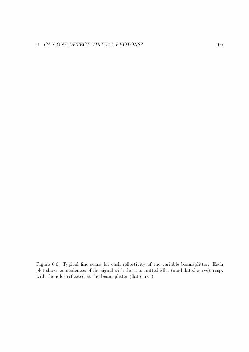
6. CAN ONE DETECT VIRTUAL PHOTONS? 105
Figure 6.6: Typical fine scans for each reflectivity of the variable beamsplitter. Eachplot shows coincidences of the signal with the transmitted idler (modulated curve), resp.with the idler reflected at the beamsplitter (flat curve).

106 6. CAN ONE DETECT VIRTUAL PHOTONS?
presented above. For the Reff = 11% the coincidences give a visibility of about 3.3%
±3.3%, the singles 0.5% ±0.3%. The latter value deviates from zero by more than a
standard deviation. But the value is so small that this deviation is not significant. The
results for the next reflectivity (Reff = 20% see Fig.6.8) are similar: 2.2% ±2.5% for
the coincidences and 0.05% ±0.1% for the singles.
In conclusion we would like to point out that our experiment confirms the interfer-
ometric model for the railcross experiment. At least for these experiments we found
that suppression and enhancement of the spontaneous emission are completely due to
destructive and constructive interference between two possibilities for the photon pair
to be emitted into a certain pair of modes. The intrinsic emission probability into the
modes between crystal and mirrors seems not to be changed by the presence of mirrors.
However the question still remains open whether this picture may be applied also to the
case of an atom and a mirror. Fearn et al.[Fearn95a] made a full quantum mechanical
calculation for the first experiment we have proposed, namely whether one can see pho-
tons immediately if one replaces the mirror suddenly by a detector. On the one hand
this result seems to support our interferometric interpretation, but the application of
their results to the second experiment is still not yet clear. In particular their model
apparently predicts a phase dependence of the emission rate observable through the mir-
ror. There, the emission probability seems to be changed by the presence of the mirror.
A full theory of this experiment is still missing. Therefore the question is still open to
which extent the interferometric picture can be applied to the atom experiment.
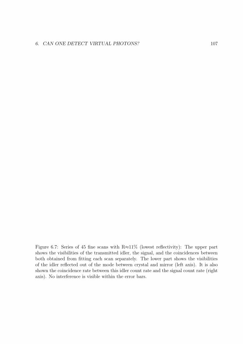
6. CAN ONE DETECT VIRTUAL PHOTONS? 107
Figure 6.7: Series of 45 fine scans with R≈11% (lowest reflectivity): The upper partshows the visibilities of the transmitted idler, the signal, and the coincidences betweenboth obtained from fitting each scan separately. The lower part shows the visibilitiesof the idler reflected out of the mode between crystal and mirror (left axis). It is alsoshown the coincidence rate between this idler count rate and the signal count rate (rightaxis). No interference is visible within the error bars.
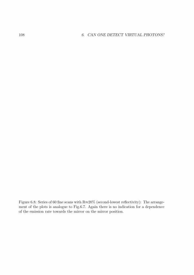
108 6. CAN ONE DETECT VIRTUAL PHOTONS?
Figure 6.8: Series of 60 fine scans with R≈20% (second-lowest reflectivity): The arrange-ment of the plots is analogue to Fig.6.7. Again there is no indication for a dependenceof the emission rate towards the mirror on the mirror position.
“There is a theory which states that if everanyone discovers what the universe is for andwhy it is here, it will instantaneously disap-pear and be replaced by something even morebizarre and inexplicable.”
(Douglas Adams in ”‘The restaurant at theend of the universe)
7 Conclusions and Outlook
Looking back to the preceding pages we want to emphasize the extraordinary character
of spontaneous parametric downconversion as a source of nonclassical light. The peculiar
correlation properties of the created photon pairs allow experiments that throw new light
on very fundamental problems of quantum mechanics and give some new insight into
the physics.
This work was mainly concerned with novel two-photon interference phenomena that
occur within PDC. By arranging mirrors in a suitable way around a nonlinear LiIO3-
crystal we realized a situation where emission into a certain pair of modes can occur via
two possible ways. If these possibilities become indistinguishable, interference between
these two emission processes occurs. One may say that we manipulate the inherent
emission process into these modes. Fringes appear in our “railcross”-setup already in
first order in contrast to most of the earlier experiments. Therefore our results cannot
directly interpreted in terms of nonlocality of quantum mechanics. However the signa-
ture of nonlocality is still present because both the signal- and idler-count rates depends
on the sum of respective phases. Furthermore we were able to show that there exists
no classical model to explain quantitatively all the features which we observed. There-
fore the conclusion seems appropriate that we are dealing with two-photon interference
phenomenon.
109

110 7. CONCLUSIONS AND OUTLOOK
How can the experiment be improved? To increase the visibility (particular in the
singles) further it is necessary to better define the modes. The best way to do this is to
use spatial filters. Then, however, one has to pay the price of a drastically reduce count
rate. One possibility to enhance the count rate is to place the nonlinear crystal inside a
cavity which is resonant for UV. We have in shown chapter 3 that one can increase the
UV power by a factor of 100 without parametric amplification to set in. The use of a
cavity makes it possible to use frequency doubled diode lasers as a pump for parametric
dowmconversion. This way one could establish a compact and cheap source of correlated
photon pairs.
A further possibility is to extend our experiment by using cavities for the signal
and idler mode. It would be quite interesting to investigate in this case the correlation
properties of the generated light. Particularly, the range just below and above the to a
parametric oscillator would be quite challenging because the physics there is not very
well known.
In a further experiment we showed that the railcross setup serves also as a useful
tool to investigate really fundamental problems in the realm of quantum mechanics.
The meaning of complementarity of interference and which-path information was the
subject of a series of experiments. We performed the first experimental demonstration
of an optimal quantum eraser. By “optimal” we mean that one need not “touch” the
interfering particle to make the interfering paths distinguishable. To accomplish this
we made use of the fact that in PDC the photons are always created in pairs. One of
the photons within a pair can serve as a quantum marker to label its conjugate photon
that constitutes the interfering system. Exactly such a situation is realized within the
railcross experiment.
In this arrangement which-path information was carried by a system (e.g. the signal)
spatially separated from the interfering system (e.g. the idler). Different degrees of
freedom (polarization and time) of the measuring photon were used to establish the
quantum marker. No manipulations were made directly on the interfering system. The
experiments confirm explicitly Feynman’s statement that one does not need carry out
the which-path measurement in reality. It is sufficient if one has the possibility for
performing it. Nevertheless interference is lost. On the other hand it turned out if
7. CONCLUSIONS AND OUTLOOK 111
the measurement is not made, that the loss of interference is reversible in complete
agreement with von Neumann’s interpretation of a quantum mechanical measurement.
Furthermore by performing a careful measurement at our which path detector we were
able to erase the which-path information again and to recover interference again upon
correlation with the interfering particle. Finally we point out that the setup could be
readily extended to demonstrate a delayed choice version. This would demonstrate in
a striking way Wheeler’s statement that “no elementary phenomenon is a phenomenon
until it is a registered (observed) phenomenon.”
In the last experiment we investigated a completely different problem. We exploited
the analogy of the railcross setup with certain experiments concerning the modification
of spontaneous emission of atoms in the vicinity of mirrors. Within the realm of cavity-
QED, the notion of vacuum is used usually to interpret these effects. Spontaneous
emission is stimulated by the presence of vacuum fluctuations. The influence of the
mirrors modifies, according to this interpretation, the emission probability of the atom
by changing the spectral distribution of the vacuum fluctuations that couple to the atom.
This picture thus led us to the conclusion that the state of the field between atom and
mirror depends on the position of the mirror. Furthermore one may test the state of the
field there by suddenly replacing the mirror by a detector. Intuitively on may expect
that the instantaneous emission rate should depend on the position of the mirror with
respect to the atom.
We have proposed a different interpretation the alteration of sponateous emission.
The atom has two possibilities to emit the photon into a certain mode, directly or via
a relection from the mirror. In this picture interference should be responsible for the
observed alteration of the emission rate. With other words the emission in this picture
is not altered but becuase of interference it appears to have been altered. This can
be demonstrated by replacing the mirror by a detector, then as opposed to the vacuum
picture, photons can immediately appear with a rate which is independent on the mirror
position.
Experiments of this kind are hard to perform with atoms, but we found that the
railcross setup can be extended to test both interpretations. The (in principle) arbitrarily
long distance of the mirrors from the crystal allows the placement of an ultrafast switch

112 7. CONCLUSIONS AND OUTLOOK
into the mode there. For the case of of emission suppression one can test for the presence
of photons between crystal and mirror.
Actually we performed an easier test. We used a variable beamsplitter to test the
field. If the reflectivity is weak enough, it should not disturb it too much. According to
the conventional interpretation one should observe a dependence of the count rate in the
mode reflected at this beamsplitter in contrast to the prediction of the interferometric
picture. In fact we did not see such a dependence.
However there are still open questions that are worthwhile to explore further. The
most important one is how to apply the interferometric picture correctly to the case of
an atom and a mirror. In the case of PDC this view gives the right answer as shown
experimentally. In the case of the atom, the right interpretation is not yet clear. An
experimental test would help to clarify the situation. It is perhaps possible that quantum
wells or excitons allow tests that are similar to the one we have performed with PDC.
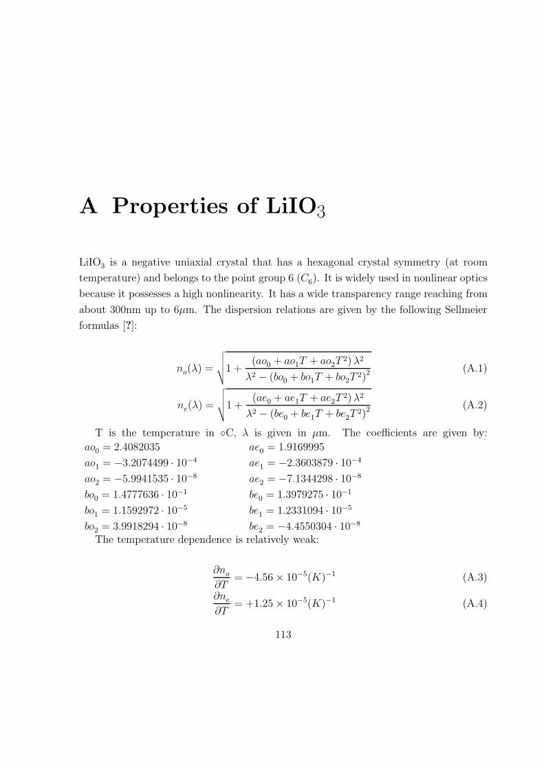
A Properties of LiIO3
LiIO3 is a negative uniaxial crystal that has a hexagonal crystal symmetry (at room
temperature) and belongs to the point group 6 (C6). It is widely used in nonlinear optics
because it possesses a high nonlinearity. It has a wide transparency range reaching from
about 300nm up to 6µm. The dispersion relations are given by the following Sellmeier
formulas [?]:
no(λ) =
√√√√1 +(ao0 + ao1T + ao2T
2)λ2
λ2 − (bo0 + bo1T + bo2T2)2 (A.1)
ne(λ) =
√√√√1 +(ae0 + ae1T + ae2T
2)λ2
λ2 − (be0 + be1T + be2T2)2 (A.2)
T is the temperature in C, λ is given in µm. The coefficients are given by:
ao0 = 2.4082035 ae0 = 1.9169995
ao1 = −3.2074499 · 10−4 ae1 = −2.3603879 · 10−4
ao2 = −5.9941535 · 10−8 ae2 = −7.1344298 · 10−8
bo0 = 1.4777636 · 10−1 be0 = 1.3979275 · 10−1
bo1 = 1.1592972 · 10−5 be1 = 1.2331094 · 10−5
bo2 = 3.9918294 · 10−8 be2 = −4.4550304 · 10−8
The temperature dependence is relatively weak:
∂no
∂T= −4.56× 10⁻⁵(K)−1 (A.3)
∂ne
∂T= +1.25× 10⁻⁵(K)−1 (A.4)
113
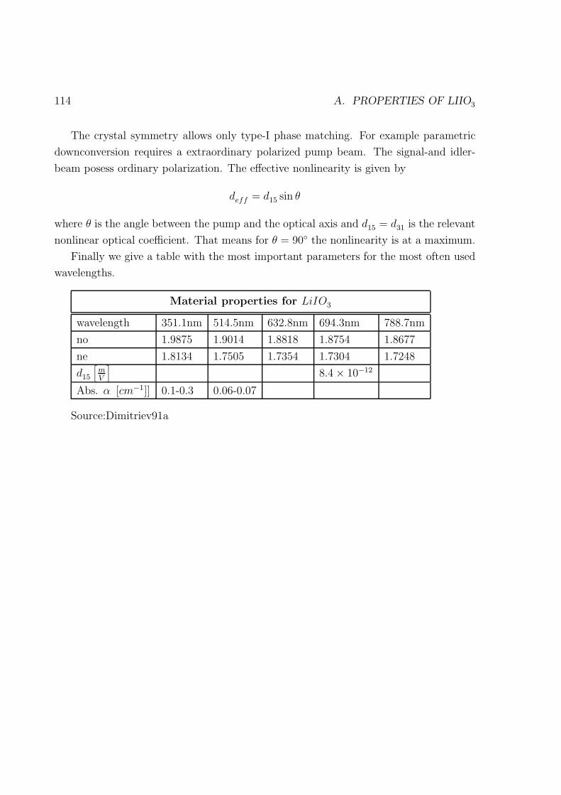
114 A. PROPERTIES OF LIIO3
The crystal symmetry allows only type-I phase matching. For example parametric
downconversion requires a extraordinary polarized pump beam. The signal-and idler-
beam posess ordinary polarization. The effective nonlinearity is given by
deff = d15 sin θ
where θ is the angle between the pump and the optical axis and d15 = d31 is the relevant
nonlinear optical coefficient. That means for θ = 90 the nonlinearity is at a maximum.
Finally we give a table with the most important parameters for the most often used
wavelengths.
Material properties for LiIO3
wavelength 351.1nm 514.5nm 632.8nm 694.3nm 788.7nm
no 1.9875 1.9014 1.8818 1.8754 1.8677
ne 1.8134 1.7505 1.7354 1.7304 1.7248
d15
[mV
]8.4× 10⁻¹²
Abs. α [cm−1]] 0.1-0.3 0.06-0.07
Source:Dimitriev91a
B The detector
We used throughout all experiments Si-avalanche photodiodes operated 20-25V above
the breakdown voltage which is typically of the order of 150-200 V. In this mode (Geiger
mode) an incoming single photon can create electron-hole pair. This photoelectron can
trigger an avalanche pulse of about 108 carriers. This current pulse is transformed by a
resistor into a voltage pulse that can be detected easily. Because the electron-avalanche
sustains itself it is necessary to suppress the avalanche by a suitable external circuit.
In our detectors we used the so-called passive quenching method [Brown86a]. Fig. B.1
shows the electronic circuit that we have used. The current is limited by a high-ohmic
resistor below about 50 µA. In this case the diode becomes again non conductive aftre
a few ns. The main drawback of this method is the long dead time of the device which
is determind by the recharging time of the diode (several µs). Therefore the maximum
count rate is limited to about 200000 cps. We mention only in passing that this drawback
can in principle be avoided by using more sophisticated electronics which is known as
“active quenching” [?, Brown87a].
In our Experiments we used two different models of avalanche photodiodes C30902S
and C30921S both manufactured by EG&G (the former producer was RCA). Both types
contain the same Si chip. The only difference is that the latter is equipped with light
pipes (multimode fiber with core diameter ≈ 250µm). These fiber detectors have a
much lower dark count rate (30-50 cps in comparison to at least 300 cps for the non
fiber detectors). We used Peltier elements to cool down the temperature to about −30
downto −40, the temperature was measured with a temperature depending resistor
(PT100). The dark count rate decreases by more than two order of magnitudes for these
115

116 B. THE DETECTOR
low temperatures. For further details on the detectors we refer to [Denifl93a].
Finally one should say a few words about the efficiency of the detectors. In principle
one should expect a intrinsic photodetection efficiency of about 40% - 50%. In reality
the efficiency was limited to about 1%. First of all there are several additional optical
elements in front of the detector: a lens to focus the light onto the sensitive area, an
interference filter and a cutoff filter to block the UV-light. But there are also effects due
to imperfect phasematching and the finite divergency of the pump beam which reduce
the efficiency strong. Both effects has been examined in detail in [Kwiat93g, Michler94a]
Figure B.1: Electronic circuit to passive quench a avalanche photodiode: In the ex-periment we choosed for the load resistor RL = 390Ω. The avalanche pulse has beendetected at the resistor RS = 50Ω.

C General theory of parametric
downconversion
An extensive description of the theory of parametric downconversion has been given in
[Mollow73a, Hong85a]. Here we will only summarize it. We start with the following
expansion of the nonlinear polarization:
Pi = χLijEj + χNL
ijk EjEk + . . .
The contributing pump-, signal- and idler fields inside the crystal have to be taken
into account. The first term describes linear effects such as refraction and dispersion, the
next term second order effects such as second harmonic generation, parametric oscillation
and so on. Here we concentrate on the second term. Then we can write for the interaction
hamiltonian
HI =1
2
∫d3r P (r) E(r) =
1
2
∫d3rχijk(r)Ei(r)Ej(r)Ek(r) (C.1)
In order to include the spontaneous parametric downconversion process, we have to
quantize the signal- and idler fields. For the positive and the negative frequency parts
of the various electric field operators it follows:
E(+)
=
(E
(−))†
=1
(2π)32
∑s
∫dk√
hω2ε0V
ε(k, s)a(k, s)ei(kr−ω(k)t) (C.2)
ε(k, s) denotes the polarization direction and a(k, s) the annihilation operator of the field.
V is the volume of the interaction region. Because of its high intensity we assume the
117
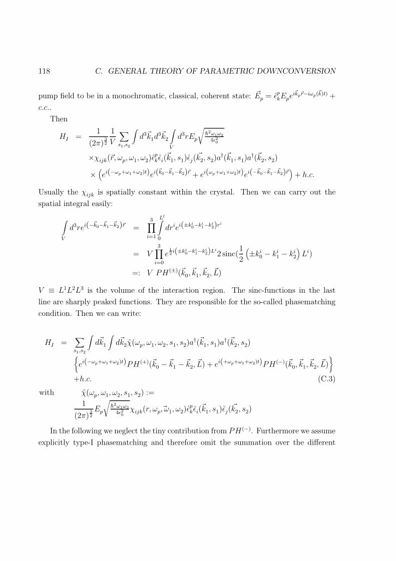
118 C. GENERAL THEORY OF PARAMETRIC DOWNCONVERSION
pump field to be in a monochromatic, classical, coherent state: Ep = εpkEpeikpr−iωp(k)t) +
c.c..
Then
HI =1
(2π)32
1
V
∑s1,s2
∫d3k1d
3k2
∫V
d3rEp
√h2ω1ω2
4ε20
×χijk(r, ωp, ω1, ω2)εpk εi(
k1, s1)εj(k2, s2)a
†(k1, s1)a†(k2, s2)
×(ei(−ωp+ω1+ω2)t)ei(
k0−k1−k2)r + ei(ωp+ω1+ω2)t)ei(−k0−k1−k2)r
)+ h.c.
Usually the χijk is spatially constant within the crystal. Then we can carry out the
spatial integral easily:
∫V
d3rei(−k0−k1−k2)r =
3∏i=1
Ll∫0
driei(±ki0−ki1−ki2)ri
= V3∏
i=0
e12i(±ki0−ki1−ki2)Li2 sinc(
1
2
(±ki0 − ki1 − ki2
)Li)
=: V PH(±)(k0,k1,
k2,L)
V ≡ L1L2L3 is the volume of the interaction region. The sinc-functions in the last
line are sharply peaked functions. They are responsible for the so-called phasematching
condition. Then we can write:
HI =∑s1,s2
∫dk1
∫dk2χ(ωp, ω1, ω2, s1, s2)a
†(k1, s1)a†(k2, s2)
ei(−ωp+ω1+ω2)t)PH(+)(k0 − k1 − k2,L) + ei(+ωp+ω1+ω2)t)PH(−)(k0,
k1,k2,
L)
+h.c. (C.3)
with χ(ωp, ω1, ω2, s1, s2) :=
1
(2π)32
Ep
√h2ω1ω2
4ε20χijk( r, ωp, ω1, ω2)ε
pk εi(
k1, s1)εj(k2, s2)
In the following we neglect the tiny contribution from PH (−). Furthermore we assume
explicitly type-I phasematching and therefore omit the summation over the different

C. GENERAL THEORY OF PARAMETRIC DOWNCONVERSION 119
polarizations. We start with the vacuum |vac〉 as input state. Then we can use first-
order perturbation theory to calculate time evolution in the interaction-picture:
|Ψ(t)〉 = exp
− i
h
t∫0
dt′HI(t′)
|vac〉 ≈ |vac〉 − i
h
t∫0
dt′HI(t′)|vac〉 (C.4)
Plugging HI into equation (C.4) we can carry out the time integral to obtain for the
state vector:
|Ψ(t)〉 = |vac〉+∫
dk1
∫dk2χ(ωp, ω1, ω2, s1, s2)a
†(k1, s1)a†(k2, s2)
PH(+)(k0,k1,
k2,L)PH(+)(ωp, ω1, ω2,
L
c) + h.c. (C.5)
where PH (+) is the same as above where frequencies has been substituted for wavevec-
tors. The time t has the meaning of the interaction time within the crystal which is given
by the coherence time of the pump beam. In most cases it is justified to assume perfect
phasematching and to substitute the sinc-functions by δ-functions assuming L →∞ and
t →∞. The k-integrals can be replaced by frequency-integrals if we confine ourself to a
single spatial mode. We end up with the two-photon state in the final form:
|Ψ〉 = |vac〉 − i
h
∫dωsdωiχ(ωp, ωs, ωi)δ(ωp − ωs − ωi)|ωs〉|ωi〉 (C.6)
This result can be genaralized easily to a finite pump bandwidth. We obtain (v(ωp)isthespectraldis
|Ψ〉 = |vac〉 − i
h
∫dωpv(ωp)
∫dωsdωiχ(ωp, ωs, ωi)δ(ωp − ωs − ωi)|ωs〉|ωi〉 (C.7)

D Standard photodetection theory
Here we summarize the rigorous photodetection theory. A more detailed analysis can
be found in any standard textbook on quantum optics (e.g. [Loudon83a]). In order
to calculate single- and coincidence count rate we make use of the Glauber correlation
function formalism [Glauber63a]. We start with an arbitrary state Ψ to describe our
system which involves two field modes. The negative and positive frequency parts of the
electric field operator can be written as1:
E(+)s (t) =
∫dω′se
iω′stηs(ωs‘)as(ω′s)
E(+)i (t) =
∫dω′ie
iω′itηi(ωi‘)ai(ω′i) (D.1)
E(−)s (t) =
(E(+)
s (t))†
E(−)i (t) =
(E
(+)i (t)
)†(D.2)
Here ηs and ηi are functions that describe effects due to filtering (by interference
filters or pinholes). The signal- and idler-singles count rate now can be calculated using
the formula:
1For convenience we stay with the names signal and idler and the corresponding subscripts
120

D. STANDARD PHOTODETECTION THEORY 121
RS\I =
T2∫
−T2
dtG(1)s\i(t) with G
(1)s\i(t) = 〈Ψ|E(−)
s\i (t)E(+)s\i (t)|Ψ〉 (D.3)
whereas G(1) describes the first-order correlation function that is responsible for first
order interference effects. This quantity is identical more or less to the intensity. Now
we show how to calculate the coincidence count rate that essentially the second order
correlation function:
RC =
T2∫
−T2
dts
ts+∆T2∫
ts−∆T2
dtiG(2)(ts, ti; ti, ts) (D.4)
with G(2)(ts, ti; ti, ts) = 〈Ψ|E(−)s (ts)E
(−)i (ti)E
(+)i (ti)E
(+)s (ts)|Ψ〉
Here ∆T denotes the coincidence time window. In practice the measurement time T
for any data point is of the order of seconds and can be assumed as infinite. Furthermore
the window ∆T is with about 5 ns also much larger than the relevant correlation time
of the photons hitting the detector (≈ several 100 fs). Therefore ∆T can be taken as
infinite as well. Now R∫\〉 and RC simplify to:
RS\I =
∞∫−∞
dtG(1)(t, t) (D.5)
RC =
∞∫−∞
dts
∞∫−∞
dtiG(2)(ts, ti; ti, ts) (D.6)
With these formulas we can calculate every count neede for this thesis. Often we
do not need to carry out the full multimode calculation in order to grasp the physics.
Instead, the main features can be understood within a simple single-mode treatment.
Then eq. (D.3) and (D.5) can be replaced by:

122 D. STANDARD PHOTODETECTION THEORY
RS/I = 〈Ψ|a†S/IaS/I |Ψ〉 (D.7)
RC = 〈Ψ|a†Sa†IaIaS|Ψ〉 (D.8)
Finally we briefly treat how to include polarization. The field operators have to be gen-
eralized to vector operators, ayj = a†j,Hεj,H+a†j,V εj,V , where εj,H, εj,V are the polarization-
basis vectors and j=S,I for the corresponding mode. Then the singles count rates can
be obtained from:
RS/I = 〈Ψ|ayS=IaS=I |Ψ〉 (D.9)
= 〈Ψ|(a†S/I,HaS/I,H + a†S/I,V aS/I,V
)|Ψ〉 (D.10)
Similarly one obtains for the coincidence rate:
RC = 〈Ψ|aySayIaIaS|Ψ〉 (D.11)
= 〈Ψ|(a†S,HaS,H + a†S,V aS,V
) (a†I,HaI,H + a†I,V aI,V
)|Ψ〉 (D.12)

E Multimode treatment of the
railcross-experiment
Our goal is to derive the eq. 3.6 and 3.9 within a multimode theory. We start from the
state
|Ψ〉 = |vac〉+α
∫dωpv(ωp)
∫dωi
∫dωsδ(ωp − ωi − ωs)f
s1 (ωs)f
i1(ωi)|ωs〉s1
|ωi〉i1+α
∫dωpv(ωp)e
iωpτp
∫dωi
∫dωsδ(ωp − ωi − ωs)f
s2 (ωs)f
i2(ωi)|ωs〉s2
|ωi〉i2(E.1)
The two terms describe the two possibilities for the PDC process to occur. α is a
number which describes the efficiency of the downconversion process, τp is the time the
pump-photon travels between these two processes. v(ωp) = ape(ωp0−ωp)2
2σ2p is the spectral
distribution of the pump. f s1 , f
i1, f
s2 , f
i2 are filter-like functions (centered around ωs0
resp. ωi0) which describes the frequency-range of the corresponding mode. Frequency-
mismatch (e.g. by a misaligned mirror) is also included. By putting s1 → s2 = s and
i1 → i2 = i we obtain:
|Ψ〉 = |vac〉+ α∫
dωpv(ωp)∫
dωi
∫dωsδ(ωp − ωi − ωs)|ωs〉s|ωi〉i
×f s
1 (ωs)fi1(ωi)e
i(ωsτs+ωiτi) + f s2 (ωs)f
i2(ωi)e
iωpτp
(E.2)
123
124 MULTIMODE TREATMENT OF THE RAILCROSS-EXP.
Here we have introduced τs and τi, the traveling times for the signal- and idler-photon,
respectively, between the two processes.
Now using the state of eq. E.2 we can calculate the single- and coincidence count
rates as follows. The signal- and idler-field operators can be written as
E(+)s (t) =
∫dω′se
iω′stηs(ωs‘)as(ω′s)
E(+)i (t) =
∫dω′ie
iω′itηi(ωi‘)ai(ω′i) (E.3)
where ηs/i(ωs/i) are the functions that describe the signal/idler interference filters. Then
|ηs/i(ωs/i)|2 ∝ e−4 ln 2
(ωs0/i0−ωs/i)2
∆ω2s/i gives the probability to find a photon with a given
frequency behind the filter (∆ωs/i gives the bandwidth). The different singles rates can
be worked out with the formula (see also appendix D):
RS\I =
T2∫
−T2
dtPs\i(t) with Ps\i(t) = 〈Ψ|E(−)s\i (t)E
(+)s\i (t)|Ψ〉 (E.4)
T denotes the duration time of a measurement. We calculate now the signal-singles rate
(the idler rate goes analogous): First let us calculate the term E(+)s (t)|Ψ〉:
E(+)s (t)|Ψ〉 = α
∫dω′se
−iω′stηs(ω′s)∫
dωpv(ωp)eiωpτp
∫dωi
∫dωsδ(ωs + ωi − ωp)
×f s
1 (ωs)fi1(ωi)e
i(ωsτs+ωiτi−ωpτp) + f s2 (ωs)f
i2(ωi)
as(ω
′s)|ωs〉s︸ ︷︷ ︸
=δ(ω′s−ωs)|0〉s
|ωi〉i
= α∫
dωse−iωstηs(ωs)
∫dωpv(ωp)e
iωpτp
∫dωiδ(ωs + ωi − ωp)
×f s
1 (ωs)fi1(ωi)e
i(ωsτs+ωiτi−ωpτp) + f s2 (ωs)f
i2(ωi)
|0〉s|ωi〉i
= α∫
dωse−iωstηs(ωs)
∫dωpv(ωp)e
iωpτp
×f s
1 (ωs)fi1(ωp − ωs)e
i(ωsτs+(ωp−ωs)τi−ωpτp) + f s2 (ωs)f
i2(ωp − ωs)
|0〉s|ωp − ωs〉i

MULTIMODE TREATMENT OF THE RAILCROSS-EXP. 125
Using Eq.[E.4] with T → ∞ (because of T Tcoh, Tcoh is the coherence time of the
downconverted light) we get:
RS =∞∫−∞
PS(t)dt
= |α|2∞∫−∞
dt∫
dωs
∫dω′se
−i(ωs−ω′s)tηs(ωs)ηs(ω′s)∫
dωp
∫dω′pv(ωp)v
(ω′p)ei(ωp−ω′p)τp
×f s
1fi1e
i(ωsτs+(ωp−ωs)τi−ωpτp) + f s2f
i2
f s
1fi1e
i(ω′sτs+(ω′p−ω′s)τi−ω′pτp) + f s2f
i2
× i〈ω′p − ω′s| s〈0|0〉s︸ ︷︷ ︸
=1
|ωp − ωs〉i︸ ︷︷ ︸
=δ(ωp−ωs−ω′p+ω′s)
(E.5)
Integration over t ⇒ δ(ωs − ω′s)
δ(ωp − ωs − ω′p + ω′s)
=⇒ δ(ωp − ω′p)
Therefore eq.E.5 simplifies to:
RS = |α|2∫
dωsη2s(ωs)
∫dωp|v(ωp)|2
|f s
1 (ωs)fi1(ωp − ωs)|2 + |f s
2 (ωs)fi2(ωp − ωs)|2 +
f s1 (ωs)f
i1(ωp − ωs)f
s1 (ωs)f
i1
(ωp − ωs)e
i(ωsτs+(ωp−ωs)τi−ωpτp) + c.c.︸ ︷︷ ︸interference term
(E.6)
Now we make the following variable transformations
ωs := ωs0 + ω′s
ωp := ωp0 + ω′p
ω′s :=ω′p2
+ ω′
which gives for the interference term:∫dωp|v(ωp)|2eiωp(
τs+τi2−τp)
×∫
dω′η2s(ω
′)f s1 (ω
′)f i1(ω
′)f s2 (ω′)f i
s (ω′)eiω
′(τs−τi) + c.c.
cos(Φs0 + Φi0 − Φp0)

126 MULTIMODE TREATMENT OF THE RAILCROSS-EXP.
with Φs0/i0/p0 = ωs0/i0/p0τs0/i0/p0. Here we made an important assumption in the form
∆ωp ∆ωs or ω′p ω′s for almost all pairs ω′p, ω′s which means that the pump
bandwidth is much smaller than the bandwidth of the downconverted light. Then we
can neglect the influence of the pump bandwidth on the different filter functions that
are now centered around zero. This makes it possible to separate the two integrals. The
final result for signal-singles count rate is then (with τav ≡ τs+τi2
and the f-functions are
real):
RS = |α|2∫
dω′η2s(ω
′)∫
dω′p|v(ω′p)|2|f s
1 (ω′)f i
1(−ω′)|2 + |f s2 (ω
′)f i2(−ω′)|2
+|α|2
∫dωp|v(ωp)|2eiωp(τav−τp) × (E.7)
2∫
dω′η2s(ω
′)f s1 (ω
′)f i1(ω
′)f s2 (ω
′)f is(ω
′)eiω′(τs−τi) cos(Φs0 + Φi0 − Φp0)
Now we set for simplicity f s1 , f
i1, f
s2 and f i
2 equal to unity (perfect alignment, band-
width defined by the detectors) and we arrive at the following expression, identical to
eq. 3.6:
RS = 2|α|2∫
dωp|v(ωp)|2∫
dωη2s(ω)
+∫
dωp|v(ωp)|2eiωp(τav−τp)∫
dωη2s(ω)e
iω(τs−τi) cos(Φs0 + Φi0 − Φp0)
= 2|α|2Ipηs1 + VpV cos(Φs0 + Φi0 − Φp0)
(E.8)
with
Ip =∫
dωp|v(ωp)|2
ηs =∫
dωη2s(ω)
Vp =1
Ip
∫dωp|v(ωp)|2eiωp(τav−τp) (E.9)
V =1
ηs
∫dωη2
s(ω)eiω(τs−τi) (E.10)

MULTIMODE TREATMENT OF THE RAILCROSS-EXP. 127
One sees immediately that the visibility of the modulation in the singles count rate is
limited by the coherence length of the laser and the bandwidth of the detected photons.
However only the relative distances of the mirrors to each other are important, not the
absolute distances of the crystal to the mirror.
Now we come to the calculation of the coincidence count rate. To perform this we
use the following formula inserting again eq. E.2:
RC =
T2∫
−T2
dts
ts+∆T2∫
ts−∆T2
dtiG(2)(ts, ti; ti, ts) (E.11)
with G(2)(ts, ti; ti, ts) = 〈Ψ|E(−)s (ts)E
(−)i (ti)E
(+)i (ti)E
(+)s (ts)|Ψ〉
is the second order correlation function which describes the probability to measure at
time ts a signal-photon and at time ti a idler photon. TR is the time resolution of the
coincidence unit.
First we evaluate E(+)i (ti)E
(+)s (ts)|Ψ〉:
E(+)i (ti)E
(+)s (ts)|Ψ〉 = α
∫dω′ie
−iω′itiηi(ω′s)∫
dω′se−iω′stsηs(ω
′s)∫
dωpv(ωp)eiωpτp
∫dωi
∫dωsδ(ωs + ωi − ωp)
×f s
1 (ωs)fi1(ωi)e
i(ωsτs+ωiτi−ωpτp) + f s2 (ωs)f
i2(ωi)
ai(ω
′i)as(ω
′s)|ωi〉i|ωs〉s︸ ︷︷ ︸
=δ(ω′i−ωi)δ(ω′s−ωs)|0〉i|0〉s
= α∫
dωie−iωitiηi(ωi)
∫dωse
−iωstsηs(ωs)∫dωpv(ωp)e
iωpτpδ(ωs + ωi − ωp)
×f s
1 (ωs)fi1(ωi)e
i(ωsτs+ωiτi−ωpτp) + f s2 (ωs)f
i2(ωi)
|0〉s|0〉i
= α∫
dωpv(ωp)eiωpτp
∫dωse
−iωstsηs(ωs)e−i(ωp−ωs)tiηi(ωp − ωs)
×f s
1 (ωs)fi1(ωp − ωs)e
i(ωsτs+(ωp−ωs)τi−ωpτp) + f s2 (ωs)f
i2(ωp − ωs)
|0〉s|0〉i

128 MULTIMODE TREATMENT OF THE RAILCROSS-EXP.
The measurement time is usually several seconds. The coincidence time window is 5
ns which is much larger than the correlation time of the downconverted photons (given
by the coherence time of the photons). Therefore we can set T →∞ and ∆T →∞ and
obtain:
RC =
∞∫−∞
dts
∞∫−∞
dtiG(2)(ts, ti; ti, ts)
= |α|2∫
dωp
∫dω′pv(ωp)v
(ω′p)ei(ωp−ω′p)τp
×∞∫−∞
dti
∞∫−∞
dts
∫dωs
∫dω′se
−i(ωs−ω′s)tsηs(ωs)ηs(ω′s)
×e−i(ωp−ωs−ω′p−ω′s)tiηi(ωp − ωs)ηi(ω
′p − ω′s)
×f s
1fi1e
i(ωsτs+(ωp−ωs)τi−ωpτp) + f s2f
i2
×f s
1fi1e
i(ω′sτs+(ω′p−ω′s)τi−ω′pτp) + f s2f
i2
× i〈0|s〈0|0〉s|0〉i︸ ︷︷ ︸
=1
(E.12)
Integration over ts ⇒ δ(ωs − ω′s)
Integration over ti ⇒ δ(ωp − ωs − ω′p + ω′s)
=⇒ δ(ωp − ω′p)
This gives:
RC = |α|2∫
dωp|v(ωp)|2∫
dωsη2s(ωs)η
2i (ωp − ωs)
|f s
1 (ωs)fi1(ωp − ωs)|2 + |f s
2 (ωs)fi2(ωp − ωs)|2 +
f s1 (ωs)f
i1(ωp − ωs)f
s1 (ωs)f
i1
(ωp − ωs)e
i(ωsτs+(ωp−ωs)τi−ωpτp) + c.c. (E.13)
With the same manipulation as for the calculation of the singles-rate we arrive at eq.
3.9:

MULTIMODE TREATMENT OF THE RAILCROSS-EXP. 129
RC = 2|α|2∫
dωp|v(ωp)|2∫
dωη2s(ω)η
2i (ω)
+∫
dωp|v(ωp)|2eiωp(τav−τp)∫
dωη2s(ω)η
2i (ω)e
iω(τs−τi) cos(Φs0 + Φi0 − Φp0)
= 2|α|2Ipηsηi1 + VpV cos(Φs0 + Φi0 − Φp0)
(E.14)
with
Ip =∫
dωp|v(ωp)|2
ηs =∫
dωη2s(ω)
ηi =∫
dωη2i (ω)
Vp =1
Ip
∫dωp|v(ωp)|2eiωp(τav−τp) (E.15)
V =1
ηsηs
∫dωη2
s(ω)η2i (ω)e
iω(τs−τi) (E.16)
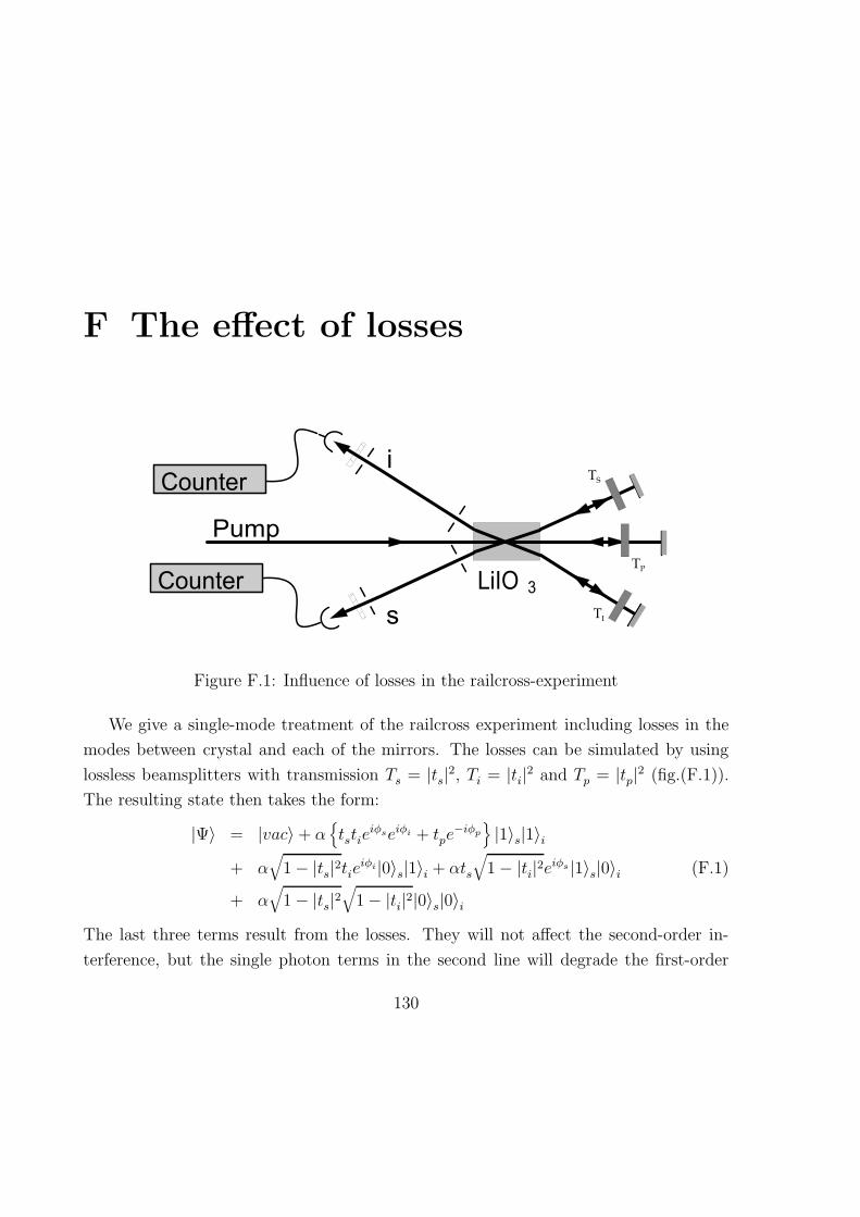
F The effect of losses
Figure F.1: Influence of losses in the railcross-experiment
We give a single-mode treatment of the railcross experiment including losses in the
modes between crystal and each of the mirrors. The losses can be simulated by using
lossless beamsplitters with transmission Ts = |ts|2, Ti = |ti|2 and Tp = |tp|2 (fig.(F.1)).
The resulting state then takes the form:
|Ψ〉 = |vac〉+ αtstie
iφseiφi + tpe−iφp
|1〉s|1〉i
+ α√1− |ts|2tieiφi|0〉s|1〉i + αts
√1− |ti|2eiφs |1〉s|0〉i (F.1)
+ α√1− |ts|2
√1− |ti|2|0〉s|0〉i
The last three terms result from the losses. They will not affect the second-order in-
terference, but the single photon terms in the second line will degrade the first-order
130
F. THE EFFECT OF LOSSES 131
visibility because they serve as an incoherent background. The last term (both photons
are lost) does not influence either measurement.
Now we can easily calculate the first- and second-order correlation functions:
Signal- and Idler-singles:
RS/I = 〈Ψ|a†s/ias/i|Ψ〉
= |α|2∣∣∣tstiei(φs+φi) + tpe
iφp∣∣∣2 + (1− |ti/s|2)|ts/i|2
= |α|2
|tsti|2 + |tp|2 + 2|tstitp| cos(φs + φi − φp) + (1− |ti/s|2)|ts/i|2
= |α|2
|ts/i|2 + |tp|2 + 2|tstitp| cos(φs + φi − φp)
(F.2)
Therefore the visibility VS/I = Max−MinMax+Min
is:
VS/I =2√TsTiTp
Ts/i + Tp
132 F. THE EFFECT OF LOSSES
Coincidences:
RC = 〈Ψ|a†ia†sasai|Ψ〉= |α|2
∣∣∣tstiei(φs+φi) + tpeiφp∣∣∣2
= |α|2|ts|2|ti|2 + |tp|2 + 2tstitp cos(φs + φi − φp)
(F.3)
=⇒ VC =2√TsTiTp
TsTi + Tp
G Calculation of the polarization
quantum eraser
We describe a general theory of the various polarization quantum erasers that we pre-
sented in chapter 5 including effects of double refraction within the nonlinear crystal or
imperfect quarter wave plates. We start from the state:
|Ψ〉 = ei∆ϕ |V 〉s |V 〉i + cos(φs) cos(φi) |V 〉s |V 〉i+ts sin(φs) cos(φi) |H〉s |V 〉i + ti cos(φs) sin(φi) |V 〉s |H〉i+tsti sin(φs) sin(φi) |H〉s |H〉i
(G.1)
ts/i := eiχs/i ∆ϕ := ϕp − ϕs − ϕi
The first term just corresponds to the direct photon pairs whereas the other four
terms arise if one turns the polarization of the reflected signal (idler) by an degree
φs (φi) and if one writes the state in the H-V-basis. Furthermore we introduced the
parameters ts, ti, mainly to describe effects of different dispersion for the H- and V-
polarization, but we can also include losses. It is straightforward to combine the results
in this appendix with those from appendix F. However the calculation is not difficult
but is quite lengthy.
G.1 Single-count rates
We want to calculate the signal-singles count rate. The action of the polarizer can be
treated with the help of the projection operator |θs〉s s 〈θs| Ψ〉:
133

134 POLARIZATION QUANTUM ERASER
=⇒∣∣∣Ψf
⟩= |θs〉s s 〈θs| Ψ〉 = cos(θs)s 〈V |+ sin(θs)s 〈H| |Ψ〉 |θs〉s
=cos(θs)
[(ei∆ϕ + cos(φs) cos(φi)) |V 〉i + ti cos(φs) sin(φi) |H〉i
]+sin(θs) [ts sin(φs) cos(φi) |V 〉i + tsti sin(φs) sin(φi) |H〉i] |θs〉s
=
[cos(θs)(e
i∆ϕ + cos(φs) cos(φi)) + ts sin(θs) sin(φs) cos(φi)]
︸ ︷︷ ︸AV
|V 〉i
+ [ti cos(θs) cos(φs) sin(φi) + tsti sin(θs) sin(φs) sin(φi)]︸ ︷︷ ︸AH
|H〉i
|θs〉s
= AV |V 〉i + AH |H〉i |θs〉s (G.2)
Then the signal-singles rate with polarizer in front of the signal detector can be
obtained with (see also Appendix D, eq. D.10):
RS =⟨Ψf
∣∣∣ (a†s,Has,H + a†s,V as,V )∣∣∣Ψf
⟩
RS =⟨Ψf
∣∣∣ (a†s,Has,H + a†s,V as,V )∣∣∣Ψf
⟩RS = s 〈θs| AV i 〈V |+ AH i 〈H| (a
†s,Has,H + a†s,V as,V ) AV |V 〉i + AH |H〉i |θs〉s
= cos2(θs)(|AV |2 + |AH |2) + sin2(θs)(|AV |2 + |AH |2) = |AV |2 + |AH |2
= | cos(θs)(ei∆ϕ + cos(φs) cos(φi)) + ts sin(θs) sin(φs) cos(φi)|2
+|ti cos(θs) cos(φs) sin(φi) + tsti sin(θs) sin(φs) sin(φi)|2
With the help of cos(∆ϕ−χs) = cos(∆ϕ) cos(χ)+sin(∆ϕ) sin(χ) we arrive at the result:
RS = A+B cos(∆ϕ) + C sin(∆ϕ) (G.3)
with:
POLARIZATION QUANTUM ERASER 135
A := cos2(θs) + cos2(θs) cos2(φs) cos
2(φi) + sin2(θs) sin2(φs) cos
2(φi)
+ cos2(θs) cos2(φs) sin
2(φi) + sin2(θs) sin2(φs) sin
2(φi)
+2 cos(θs) cos(φs) cos(φi) sin(θs) sin(φs) cos(φi) cos(χs)
+2 cos(θs) sin(θs) cos(φs) sin(φs) sin2(φi) cos(χs)
B := 2 cos2(θs) cos(φs) cos(φi) + 2 cos(θs) sin(θs) sin(φs) cos(φi) cos(χs)
C := 2 cos(θs) sin(θs) sin(φs) cos(φi) sin(χs)
We can rewrite this result in a more convenient form:
RS = A+√B2 + C2 sin
(∆ϕ+ arctan
(B
C
))(G.4)
=⇒
V is = Max−MinMax+Min
=√B2+C2
A
Mean = A
Φ0 = arctan(BC
) (G.5)
Now we regard some special cases:
1. The normal railcross experiment =⇒ φs = φi = 0 :
A = 2 cos2(θs)
B = 2 cos2(θs)
C = 0
=⇒
V is = 2 cos2(θs)2 cos2(θs)
≡ 1
Φ0 = 90
As expected there the visibility of the fringe pattern does not depend on the
polarizer angles, only the mean value varies with θs.
2. Now let us consider the setup where we turn the polarization of the signal only
=⇒ φs = 90 ∧ φi = 0 :
A = cos2(θs) + sin2(θs) = 1
B = 2 sin(θs) cos(θs) cos(χs)
C = 2 sin(θs) cos(θs) sin(χs)
=⇒ V is = sin(2θs)
Φ0 = arctan(cot(χs))(G.6)

136 POLARIZATION QUANTUM ERASER
The visibility depends on the polarizer angle θs. For θs = 0 and θs = 90 our
measurement contains which-path information. Consequently the interference van-
ishes. On the other hand if the polarizer points to 45, the origin of the detected
idler-photons photons cannot be determined and interference is restored again.
This completely agrees with the experimental results.
3. Next we treat the case of incomplete which-path information
=⇒ φs = arb. ∧ φi = 90 :
We obtain:
A = cos2(θs) + cos2(θs) cos2(φs) + sin2(θs) sin
2(φs)
+2 cos(θs) sin(θs) cos(φs) sin(φs) cos(χs)χs=0= cos2(θs) + (cos(θs) cos(φs) + sin(θs) sin(φs))
2
B = 2 cos2(θs) cos(φs) + 2 cos(θs) sin(θs) sin(φs) cos(χs)χs=0= 2 cos2(θs) cos(φs) + 2 cos(θs) sin(θs) sin(φs)
C = 2 cos(θs) sin(θs) sin(φs) sin(χs)χs=0= 0
We only consider the two special cases χ2 = 0 and χ2 = 180 of this complicated
result that simplifies now to:
V is =
χs=0= 2 cos(θs) cos(θs−φs)
cos2(θs)+cos2(θs−φs)χs=180= 2 cos(θs) cos(θs+φs)
cos2(θs)+cos2(θs+φs)
(G.7)
The visibility now depends on both θs and φs. An example for φs = 30 is plotted
in Fig. (??). The general behavior for χ = 0 shows that upon variation θs we
have two values1 where the interference can be completely restored. One lies at
θs =φs2the other one at θs = 90+ φs
2. The first angle corresponds to a direction of
the polarizer along the half angle between the polarizations of direct and reflected
1in a range from 0 to 180 since from 180 → 360 the values are identical.

POLARIZATION QUANTUM ERASER 137
signal. The other one points to the orthogonal direction of the first one. There
are two other directions where interference disappears completely, one at θs = 0
the other one at θs = φs − 90. In both cases the polarizer is exactly vertical
polarized to either the direct signal or the reflected signal. Therefore we obtain
perfect which-path information and interference is destroyed.
4. It is a simple affair to treat the case of rotating the polarization of both the signal
and idler =⇒ φs = 90 ∧ φi = 90 :
A = cos2(θs) + sin2(θs) ≡ 1
B = 0
C = 0
=⇒ V is = 0
Φ0 = 0(G.8)
Independent of the polarizer directions, first-order interference disappears com-
pletely due to the fact that the signal photons are distinguishable via the polar-
ization of the idler photons. Which-path information can only be erased by a
correlation measurement.
G.2 Coincidence count rate
Now let us turn to the calculation of the coincidence count rate A polarizer is placed in
front of each detector at an angle θs resp. θi. The state after the polarizers becomes:
=⇒∣∣∣Ψf
⟩= |θs〉s |θi〉i i 〈θi| s 〈θs| Ψ〉
with (in the H-V-basis):
|θs〉s |θi〉i ≡ cos(θs) |V 〉s + sin(θs) |H〉s cos(θi) |V 〉i + sin(θi) |H〉i
=⇒∣∣∣Ψf
⟩= cos(θs)s 〈V |+ sin(θs)s 〈H| cos(θi)i 〈V |+ sin(θi)i 〈H|i |Ψ〉 |θs〉s |θi〉i
=cos(θs) cos(θi)(e
i∆ϕ + cos(φs) cos(φi)) + ts sin(θs) cos(θi) sin(φs) cos(φi)

138 POLARIZATION QUANTUM ERASER
+ti cos(θs) sin(θi) cos(φs) sin(φi) + tsti sin(θs) sin(θi) sin(φs) sin(φi) |θs〉s |θi〉i= AC |θs〉s |θi〉i
Similarly to the singles count rates, the coincidence count rate can be obtained from
the relation (eq. D.12 in appendix D):
RC =⟨Ψf
∣∣∣ (a†s,Has,H + a†s,V as,V )(a†i,Hai,H + a†i,V ai,V )
∣∣∣Ψf
⟩= |AC |2i 〈θi| s 〈θs| (a
†s,Has,H + a†s,V as,V )(a
†i,Hai,H + a†i,V ai,V ) |θs〉s |θi〉i
= |AC |2cos2(θs) cos
2(θi) + sin2(θs) cos2(θi) + cos2(θs) sin
2(θi) + sin2(θs) sin2(θi)
= |AC |2 (G.9)
=∣∣∣cos(θs) cos(θi)(ei∆ϕ + cos(φs) cos(φi)) + ts sin(θs) cos(θi) sin(φs) cos(φi) (G.10)
+ti cos(θs) sin(θi) cos(φs) sin(φi) + tsti sin(θs) sin(θi) sin(φs) sin(φi)|2 (G.11)
After a longish calculation where we make use of the following theorems for the trigono-
metric functions
cos(α + β) = cos(α) cos(β)− sin(α) sin(β)
cos(α + β) + cos(α− β) = 2 cos(α) cos(β)
we obtain again:
RC = A′ +B′ cos(∆ϕ) + C ′ sin(∆ϕ)
= A′ +√B′2 + C ′2 sin(∆ϕ + arctan
(B′
C ′
))
=⇒
V is = Max−MinMax+Min
=√B′2+C′2
A′
Mean = A′
Φ′0 = arctan(B′
C′
) (G.12)
whereas

POLARIZATION QUANTUM ERASER 139
A′ := cos2(θs) cos2(θi)
+(cos2(θs) cos
2(φs) + sin2(θs) sin2(φs)
) (cos2(θi) cos
2(φi) + sin2(θi) sin2(φi)
)+2 cos(θs) sin(θs) cos(φs) sin(φs)
(cos2(θi) cos
2(φi) + sin2(θi) sin2(φi)
)cos(χs)
+2(cos2(θs) cos
2(φs) + sin2(θs) sin2(φs)
)cos(θi) sin(θi) cos(φi) sin(φi) cos(χi)
+4 cos(θs) sin(θs) cos(θi) sin(θi) cos(φs) sin(φs) cos(φi) sin(φi) cos(χs) cos(χi)
B′ := 2 cos2(θs) cos2(θi) cos(φs) cos(φi) + 2 cos(θs) sin(θs) cos
2(θi) sin(φs) cos(φi) cos(χs)
+2 cos2(θs) cos(θi) sin(θi) cos(φs) sin(φi) cos(χi)
+2 cos(θs) sin(θs) cos(θi) sin(θi) sin(φs) sin(φi) cos(χs + χi)
C ′ := 2 cos(θs) sin(θs) cos2(θi) sin(φs) cos(φi) sin(χs)
+2 cos2(θs) cos(θi) sin(θi) cos(φs) sin(φi) sin(χi)
+2 cos(θs) sin(θs) cos(θi) sin(θi) sin(φs) sin(φi) sin(χs + χi)
Let us regard some special cases again:
1. As a first check again the railcross experiment φs = φi = 0:
A′ = 2 cos2(θs) cos2(θi)
B′ = 2 cos2(θs) cos2(θi)
C ′ = 0
=⇒ V is = 1
2. As a second example we apply the result again to the simple case of a polarization
quantum marker directly in the interfering system (e.g. the signal) φs =
0 ∧ φi = 90 :
A′ = cos2(θs) cos2(θi) + cos2(θs) sin
2(θi) = cos2(θs)
B′ = 2 cos2(θs) cos(θi) sin(θi) cos(χi)
C ′ = 2 cos2(θs) cos(θi) sin(θi) sin(χi)
=⇒ V is = 2 cos(θi) sin(θi)
Φ0 = arctan(cot(χi))
(G.13)

140 POLARIZATION QUANTUM ERASER
Because this experiment deals essentially with first-order interference during every
step we get the same visibility as for the singles count rates.
3. The case of incomplete which-path information
⇒ φs = arb. ∧ φi = 90:
Again because we have again a first-order interference we get the same visibility
as for the singles.
V is =
χs=0= 2 cos(θs) cos(θs−φs)
cos2(θs)+cos2(θs−φs)χs=180= 2 cos(θs) cos(θs+φs)
cos2(θs)+cos2(θs+φs)
(G.14)
4. Most interesting is the case where the polarization of both the directed signal and
idler photons is rotated by 90, the polarization- (or spin-) entangled case with
φs = 90 ∧ φi = 90:
A′ = cos2(θs) cos2(θi) + sin2(θs) sin
2(θi)
B′ = 2 cos(θs) sin(θs) cos(θi) sin(θi) cos(χs + χi)
C ′ = 2 cos(θs) sin(θs) cos(θi) sin(θi) sin(χs + χi)
=⇒
V is = 2 cos(θs) sin(θs) cos(θi) sin(θi)cos2(θs) cos2(θi)+sin2(θs) sin2(θi)
Φ0 = arctan(cot(χs + χi))
Obviously, interference can be obtained in coincidence only for θs = θi = 45,
i.e. if the polarizer are at the half angle between both contributing polarizations2.
We have now truly second-order interference because the singles do not show a
modulation as we have found above. On the other hand for θs = θi = 0 or
θs = θi = 90 the measurement yields which-path for the detected photon pairs,
and therefore interference disappears.
5. As a last remark we consider two special settings of the phase ∆ϕ (again with
φs = 90 ∧ φi = 90):
2Note that the fringe pattern visible in the signal-, idler- coincidence-count rate are subject todifferent phase shifts, χs for the signal, χi for the idler and χs + χs for the coincidences. This featurehas been observed in the experiment.
POLARIZATION QUANTUM ERASER 141
RC = cos2(θs) cos2(θi) + sin2(θs) sin
2(θi) + 2 cos(θs) sin(θs) cos(θi) sin(θi) cos(∆ϕ)
=
(cos(θs) cos(θi) + (θs) sin(θi))
2 = (cos(θs + θi))2 ⇐⇒ ∆ϕ = 0
(cos(θs) cos(θi)− (θs) sin(θi))2 = (cos(θs − θi))
2 ⇐⇒ ∆ϕ = 180(G.15)
For these special phase settings we obtain the correlation functions characteristic
for the spin-entangled states |H〉s|H〉i + |V 〉s|V 〉i and |H〉s|H〉i − |V 〉s|V 〉i [citek-wiat95b].
Acknowledgements
142
Bibliography
[Aschenwald93a] J. Aschenwald. Realisierung eines Quanten.Erasers. Master’s thesis,University Innsbruck, (1993). Innsbruck, unpublished.
[Aspect82a] A. Aspect, J. Dalibard and G. Roger. Experimental test of Bell’s in-equalities using time-varying analyzers. Phys. Rev. Lett., 49, (25),1804–1807, (1982).
[Baldzuhn89a] J. Baldzuhn, E. Mohler and W. Martienssen. A wave-particle delayed-choice experiment with a single-photon state. Z. Physik B, 77, 347–352,(1989).
[Bennett92b] C. H. Bennett, G. Brassard and A. K. Ekert. Quantum cryptography.Sci. Am., 50–57, October (1992).
[Bennett93a] C. H. Bennett, G. Brassard, C. Crepeau, R. Jozsa, A. Peres andW. K.Wootters. Teleporting an unknown quantum state via dual classi-cal and Einstein-Podolsky-Rosen channels. Phys. Rev. Lett., 70, (13),1895–1899, (1993).
[Boyd92a] Robert W. Boyd. Nonlinear Optics. Academic Press, San Diego, CA,(1992).
[Brendel91a] J. Brendel, E. Mohler and W. Martienssen. Time-resolved dual-beamtwo-photon intererences with high visibility. Phys. Rev. Lett., 66, (9),1142–1145, (1991).
[Brendel92a] J. Brendel, E. Mohler and W. Martienssen. Experimental test of Bell’sinequality for energy and time. Europhys. Lett., 20, (7), 575–580,(1992).
[Brown86a] R. G. W. Brown, K. D. Ridley and J. G. Rarity. Characterization ofsilicon avalanche photodiodes for photon correlation measurements. 1:Passive quenching. Appl. Opt., 25, (22), 4122–4126, (1986).
143

144 BIBLIOGRAPHY
[Brown87a] R. G. W. Brown, R. Jones, J. G. Rarity and K. D. Ridley. Characteri-zation of silicon avalanche photodiodes for photon correlation measure-ments. 2: Active quenching. Appl. Opt., 26, (12), 2383–2389, (1987).
[Burnham70a] D. C. Burnham and D. L. Weinberg. Observation of simultaneity inparametric production of optical photon pairs. Phys. Rev. Lett., 25,84–7, (1970).
[Casimir48a] H. B. G. Casimir. On the Attraction between Two Perfectly ConductingPlates. Proc. K. Ned. Akad. Wet., 51, 793, (1948). Casimir Effect.
[Chapman95a] M. S. Chapman, T. D. Hammond, A. Lenef, J. Schmiedmayer, R. A.Rubenstein, E. Smith and D. E. Pritchard. Photon scattering fromatoms in an atom interferometer: coherence lost and regained. submit-ted to Phys.Rev.Lett., (1995).
[Cohen-Tannoudji92a] C. Cohen-Tannoudji, J. Dupont-Roc and Gilbert Grynberg. Atom-Photon Interactions. John Wiley & Sons, inc., New York, (1992).
[Cook87a] R. J. Cook and P. W. Milloni. Quantum theory of an atom near partiallyreflecting walls. Phys. Rev. A, 35, (12), 5081–5087, (1987).
[Denifl93a] G. Denifl. Einzelphotonen-Detektoren fur Quantenkorrelations-Experimente. Master’s thesis, University Innsbruck, (1993).
[Deppe90a] D. G. Deppe, J. C., R. Kuchibhotla, T. J. Rogers and B. G. Streetman.Electron. Lett., 26, 1666, (1990).
[Dimitriev91a] V. G. Dimitriev, G. G. Gurzadyan and D. N. Nikogosyan. Handbookof nonlinear optical crystals. Springer series in optical physics, vol. 64.Springer, (1991).
[Drexhage74a] K. H. Drexhage. Progress in Optics, 12, 163, (1974).
[Einstein35a] A. Einstein, B. Podolsky and N. Rosen. Can quantum-mechanical de-scription of physical reality be considered complete? Phys. Rev., 47,777–780, (1935).
[Ekert91a] A. K. Ekert. Quantum cryptography based on Bell’s theorem. Phys.Rev. Lett., 67, (6), 661, (1991).
[Elitzur93a] A. C. Elitzur and L. Vaidman. Quantum mechanical interaction-freemeasurements. Found. Phys., 23, (7), 987–997, (1993).

BIBLIOGRAPHY 145
[Englert90a] G.-E. Englert, J. Schwinger and M. O. Scully. In A. O. Barut, editor,New Frontiers in Quantum Electrodynamics and Quantum Optics, 513–519. Plenum, New York, (1990).
[Englert94b] B.-G. Englert, H. Fearn, M. O. Scully and H. Walther. The micro-maser welcher-weg detector revisited. In F.De Martini, G.Denardo andA.Zeilinger, editors, Proc. Of the Adriatico Workshop on Quantum In-terference 1993, Trieste, Italy, 103–119. World Scientific, (1994).
[Englert94a] B.-G. Englert, M. O. Scully and H. Walther. The duality in matter andlight. Sci. Am., 56–61, December (1994).
[Fearn89a] H. Fearn and R. Loudon. Theory of two-photon interference. J. Opt.Soc. Am. B, 6, (5), 917, (1989).
[Fearn95a] H. Fearn, R. J. Cook and P. W. Milonni. Sudden Replacement of a Mirorby a Detector in Cavity QED: Are Photons Counted Immediately? Phys.Rev. Lett., 74, (8), 1327–1330, (1995).
[Feynman65a] R. P. Feynman, R. B. Leighton and M. Sands. The feynman lectures onphysics, volume III. Addison-Wesley, Reading, Massachussetts, (1965).
[Franson89a] J. D. Franson. A New Test of Bell’s Inequality Using Optical Interfer-ence. ???, ???, (???), ???, (1989).
[Gabrielse85a] G. Gabrielse and H. Dehmelt. Phys. Rev. Lett., 55, 67, (1985).
[Glauber63a] R. J. Glauber. Quantum theory of optical coherence. Phys. Rev., 130,2529, (1963).
[Goy83a] P. Goy, J. M. Raimond, M. Gross and S. Haroche. Phys. Rev. Lett.,50, 1903, (1983).
[Grangier86a] P. Grangier, G. Roger and A. Aspect. Experimental evidence for aphoton anticorrelation effect on a beam splitter: a new light on single-photon interferences. Europhys. Lett., 1, (4), 173–179, (1986).
[Hardy92a] L. Hardy. Quantum mechanics, local realistic theories, and Lorentz-invariant realistic theories. Phys. Rev. Lett., 68, (20), 2981–2984.
[Haroche89a] S. Haroche and D. Kleppner. Physics Today, 25, January (1989).
[Haroche92a] S. Haroche, M. Brune and J. M. Raimond. Manipulations of opti-cal fields by atomic interferometry: quantum variations on a theme byYoung. Appl. Phys. B, 54, 355–365, (1992).

146 BIBLIOGRAPHY
[Hecker95a] N. Hecker, R.Rodrigues-Herzog and R. HOpfel. private communication.
[Heinzen87a] D. Heinzen, J. J. Childs, J. E. Thomas and M. S. Feld. Phys. Rev.Lett., 58, 1320, (1987).
[Hellmuth87a] T. Hellmuth, H. Walther, A. Zajonc and W. Schleich. Delayed-choiceexperiments in quantum interference. Phys. Rev. A, 35, (6), 2532–2541,(1987).
[Herzog94b] T. J. Herzog, J. G. Rarity, H. Weinfurter and A. Zeilinger. Frustratedtwo-photon creation via interference: Reply. Phys. Rev. Lett., 73, (22),3041, (1994).
[Herzog94a] T. J. Herzog, J.G. Rarity, H. Weinfurter and A. Zeilinger. Frustratedtwo-photon creation via interference. Phys. Rev. Lett., 72, (5), 629–632,(1994).
[Hinds90a] E. H. Hinds. ??????? volume 28 of Advances in Atomic, Molecularand Optical Physics, 111111. Academic Press, Boston, (1990). ed. D.R.Bates and B. Bederson.
[Hong85a] C. K. Hong and L. Mandel. Theory of parametric frequency down con-version of light. Phys. Rev. A, 31, (4), 2409, (1985).
[Hong87a] C. K. Hong, Z. Y. Ou and L. Mandel. Measurement of subpicosecondtime intervals between two photons by interference. Phys. Rev. Lett.,59, (18), 2044, (1987).
[Horne89a] M. Horne, A. Shimony and A. Zeilinger. Two-particle interferometry.Phys. Rev. Lett., 62, (19), 2209–2212, (1989).
[Hulet85a] R. G. Hulet, E. S. Hilfer and D. Kleppner. Phys. Rev. Lett., 55, 2137,(1985).
[Jhe87a] W. Jhe, A. Anderson, E. A. Hinds, D. Meschede, L. Moi and S. Haroche.Phys. Rev. Lett., 58, 666, (1987).
[Klyshko80a] D. N. Klyshko. Sov.J.Quantum Electron., 10, 1112, (1980).
[Kwiat90a] P. G. Kwiat, W. A. Vareka, C. K. Hong, H. Nathel and R. Y. Chiao.Correlated two-photon interference in a dual-beam Michelson interfer-ometer. Phys. Rev. A, 41, (5), 2910, (1990).

BIBLIOGRAPHY 147
[Kwiat91a] P. G. Kwiat and R. Y. Chiao. Observation of a nonclassical Berry’sphase for the photon. Phys. Rev. Lett., 66, (5), 588–591, (1991).
[Kwiat92b] P. G. Kwiat, Ae. M. Steinberg and R. Y.Chiao. Observation of a ‘quan-tum eraser’: a revival of coherence in a two-photon interference exper-iment. Phys. Rev. A, 45, (11), 7729, (1992).
[Kwiat93g] P. G. Kwiat. Nonclassical Effects from Spontaneous Parametric Down-conversion: Adventures in Quantum Wonderland. PhD thesis, Univer-sity of California at Berkeley, (1993).
[Kwiat93a] P. G. Kwiat, A. M. Steinberg and R. Y. Chiao. High-visibility interfer-ence in a Bell-inequality experiment for energy and time. Phys. Rev. A,47, (4), 2472–2475, (1993). Rapid Communication.
[Kwiat95a] P. G. Kwiat, H. Weinfurter, T. Herzog, A. Zeilinger and M. A. Ka-sevich. Interaction-free measurement. accepted for publication inPhys.Rev.Lett., (1995).
[Loudon83a] R. Loudon. The quantum theory of light. Oxford University Press, 2ndedition, (1983).
[Mandel84a] L. Mandel. Proposal for almost noise-free optical communication underconditions of high background. J. Opt. Soc. Am. B, 1, (1), 108–110,(1984).
[Mattle93a] K. U. Mattle. Zweiphotonen-Quantenstatistik am Dreifachstrahlteiler.Master’s thesis, University Innsbruck, (1993). to be published as apaper.
[Michler94a] M. Michler. Photonenkorrelationen an mehrfachstrahlteilern. Master’sthesis, Inst. for Experimentalphysics, Innsbruck, (1994).
[Milonni94a] P. W. Milonni. The quantum vacuum: An introduction to quantumelectrodynamics. Academic Press, (1994).
[Milonni95b] P. W. Milonni, H. Fearn and A. Zeilinger. Theory of Two-Photon Down-conversion in the Presence of Mirrors. (1995). to be published.
[Mlynek95a] J. Mlynek. to be published. (1995).
[Mollow73a] B. R. Mollow. Phys. Rev. A, 8, 2864, (1973).

148 BIBLIOGRAPHY
[Bohr83a] N.Bohr. In J. A. Wheeler and W. H. Zurek, editors, Quantum The-ory and Measurement, 9. Princeton University Press, Princeton, NJ,(1983).
[Neumann32a] J. Von Neumann. Mathematische grundlagen der quantenmechanik.Springer, Berlin, (1932). English trans. by R. T. Beyer, Mathemati-cal Foundations of Quantumechanics, Princeton U.P., Princeton, N.J.(1955).
[Ou90a] Z. Y. Ou, L. J. Wang, X. Y. Zou and L. Mandel. Evidence for phasememory in two-photon down conversion through entanglement with thevacuum. Phys. Rev. A, 41, (1), 566, (1990).
[Ou90b] Z. Y. Ou, X. Y. Zou, L. J. Wang and L. Mandel. Observation of nonlocalinterference in separated photon channels. Phys. Rev. Lett., 65, (3),321–324, (1990).
[Kwiat94e] A. M. Steinberg P. G. Kwiat and R. Y. Chiao. Three Proposed ‘QuantumErasers’. PRA, 49, (1), 61–68, (1994).
[Pfau94a] T. Pfau, S. Sp”Alter, Ch. Kurtsiever, C. R. Ekstrom and J. Mlynek.Loss of Spatial Coherence by a Single Spontaneous Emission. Phys.Rev. Lett., 73, (9), 1223–1226, (1994).
[Purcell46a] E. M. Purcell. Phys. Rev., 69, 681, (1946).
[Rarity87a] J. G. Rarity, K. D. Ridley and P. R. Tapster. Absolute measurementof detector quantum efficiency using parametric downconversion. Appl.Opt., 26, (21), 4616–4619, (1987).
[Rarity90b] J. G. Rarity and P. R. Tapster. Experimental violation of Bell’s in-equality based on phase and momentum. Phys. Rev. Lett., 64, (21),2495–2498, (1990).
[Schilpp49a] P. A. Schilpp, editor. Albert Einstein philosopher-scientist. The libraryof living philosphers Vol. 7. Open Court, La Salle, Illinois, (1949).
[Schmiedmayer95a] J. Schmiedmayer. private communication, (1995).
[Scully82a] M. O. Scully and K. Druhl. Quantum eraser: a proposed photon corre-lation experiment concerning observation and “delayed choice” in quan-tum mechanics. Phys. Rev. A, 25, (4), 2208–2213, (1982).
BIBLIOGRAPHY 149
[Scully91a] M. O. Scully, B.-G. Englert and H. Walther. Quantum optical test ofcomplementarity. Nature, 351, 111, (1991).
[Senitzky94a] I. R. Senitzky. Frustrated Two-photon Creation via Interference: Com-ment. Phys. Rev. Lett., 73, 3040, (1994).
[Haroche92b] S.Haroche. Cavity Quantum Electrodynamics. In J.Dalibard,J.M.Raimond and J.Zinn-Justin, editors, Fundamental Systems inQuantum Optics, 767–940. Elsevier Science Publishers B.V., (1992).Les Houuches LIII, 1990.
[Steinberg92b] A. M. Steinberg, P. G. Kwiat and R. Y. Chiao. Dispersion cancellationin a measurement of the single-photon propagation velocity in glass.Phys. Rev. Lett., 68, (16), 2421–2424, (1992).
[Steinberg93a] A. M. Steinberg, P. G. Kwiat and R. Y. Chiao. Measurement of thesingle-photon tunneling time. Phys. Rev. Lett., 71, 708–711, (1993).
[Stern90a] A. Stern, Y. Aharonov and Y. Imri. Phase uncertainty and loss ofinterference: A general picture. Phys. Rev. A, 41, (7), 3436–3448,(1990).
[Storey94b] P. Storey, S. Tan, M. Collet and D. F. Walls. Path D¿etection and theUncertainty Principle. Nature, 367, 626–628, (1994).
[Tan93a] S. M. Tan and D. F. Walls. Loss of coherence in interferometry. Phys.Rev. A, 47, (6), 4663–4676, (1993).
[Weinfurter95a] H. Weinfurter, T. Herzog, P.G.Kwiat, J.G.Rarity and A.Zeilinger.Frustrated Down-Conversion: Can One Detect Virtual Photons? InD.M.Greenberger and A.Zeilinger, editors, Fundamental Problems inQuantum Theory: A Conference Held in Honor of Prof. John A.Wheeler, volume 755, 61. Annals of the New York Academy of Sci-ences, (1995).
[Wheeler79a] J. A. Wheeler. In G. T. DiFrancia, editor, Problems in the Formulationof Physics. North-Holland, Amsterdam, (1979).
[Wheeler83a] J. H. Wheeler and W. H. Zurek, editors. Quantum theory and mea-surement, Princeton, New Jersey, (1983). Princeton University Press.
[Wooters79a] W. K. Wooters and W. H. Zurek. Complementarity in the double-slitexperiment: Quantum nonseperability and a quantitative statement ofBohr’s principle. Phys. Rev. D, 19, (2), 473–484, (1979).

150 BIBLIOGRAPHY
[Wu85a] A. Wu and H. J. Kimble. J. Opt. Soc. Am. B, 2, 697, (1985).
[Yablonovitch87a] E. Yablonovitch. Phys. Rev. Lett., 58, 2059, (1987).
[Yariv89a] A. Yariv. Quantum electronics. John Wiley, New York, 3rd edition,(1989).
[Zajonc91a] A. G. Zajonc, L. J. Wang, X. Y. Zou and L. Mandel. Quantum eraser.Nature, 353, 507–508, (1991).
[Zou91a] X. Y. Zou, L. J. Wang and L. Mandel. Induced coherence and indistin-guishability in optical interference. Phys. Rev. Lett., 67, (3), 318–321,(1991).
[Zukowski95a] M. Zukowski. private communication. (1995).
[Zurek91a] W. H. Zurek. Decoherence and the transition from quantum to classical.Physics Today, 36–44, October (1991).

Curriculum Vitae
151

Publications
152