NORTH SEA STUDY OCCASIONAL PAPER

No. 126

AN OPTIMISED INVESTMENT MODEL OF THE

ECONOMICS OF INTEGRATED RETURNS

FROM CCS DEPLOYMENT IN THE UK/UKCS

Professor Alexander G. Kemp

and

Sola Kasim

May, 2013

Aberdeen Centre for Research in Energy Economics and

Finance (ACREEF) © A.G. Kemp and S. Kasim

i

ISSN 0143-022X

NORTH SEA ECONOMICS

Research in North Sea Economics has been conducted in the Economics Department

since 1973. The present and likely future effects of oil and gas developments on the

Scottish economy formed the subject of a long term study undertaken for the Scottish

Office. The final report of this study, The Economic Impact of North Sea Oil on

Scotland, was published by HMSO in 1978. In more recent years further work has

been done on the impact of oil on local economies and on the barriers to entry and

characteristics of the supply companies in the offshore oil industry.

The second and longer lasting theme of research has been an analysis of licensing and

fiscal regimes applied to petroleum exploitation. Work in this field was initially

financed by a major firm of accountants, by British Petroleum, and subsequently by

the Shell Grants Committee. Much of this work has involved analysis of fiscal

systems in other oil producing countries including Australia, Canada, the United

States, Indonesia, Egypt, Nigeria and Malaysia. Because of the continuing interest in

the UK fiscal system many papers have been produced on the effects of this regime.

From 1985 to 1987 the Economic and Social Science Research Council financed

research on the relationship between oil companies and Governments in the UK,

Norway, Denmark and The Netherlands. A main part of this work involved the

construction of Monte Carlo simulation models which have been employed to

measure the extents to which fiscal systems share in exploration and development

risks.

Over the last few years the research has examined the many evolving economic issues

generally relating to petroleum investment and related fiscal and regulatory matters.

Subjects researched include the economics of incremental investments in mature oil

fields, economic aspects of the CRINE initiative, economics of gas developments and

contracts in the new market situation, economic and tax aspects of tariffing,

economics of infrastructure cost sharing, the effects of comparative petroleum fiscal

systems on incentives to develop fields and undertake new exploration, the oil price

responsiveness of the UK petroleum tax system, and the economics of

decommissioning, mothballing and re-use of facilities. This work has been financed

by a group of oil companies and Scottish Enterprise, Energy. The work on CO2

Capture, EOR and storage was financed by a grant from the Natural Environmental

Research Council (NERC) in the period 2005 – 2008.

For 2013 the programme examines the following subjects:

a) Refining/Streamlining the Field Allowances for SC

b) Economics of Exploration in the UKCS: the 2013 Perspective

c) Third Party Access to Infrastructure

d) Economics of EOR in UKCS

e) Economics of CO2 EOR

f) Prospects for Activity Levels in the UKCS: the 2013 Perspective

ii

g) Economics of Issues Relating to Decommissioning

The authors are solely responsible for the work undertaken and views expressed. The

sponsors are not committed to any of the opinions emanating from the studies.

Papers are available from:

The Secretary (NSO Papers)

University of Aberdeen Business School

Edward Wright Building

Dunbar Street

Aberdeen A24 3QY

Tel No: (01224) 273427

Fax No: (01224) 272181

Email: a.g.kemp@abdn.ac.uk

Recent papers published are:

OP 98 Prospects for Activity Levels in the UKCS to 2030: the 2005

Perspective

By A G Kemp and Linda Stephen (May 2005), pp. 52

£20.00

OP 99 A Longitudinal Study of Fallow Dynamics in the UKCS

By A G Kemp and Sola Kasim, (September 2005), pp. 42

£20.00

OP 100 Options for Exploiting Gas from West of Scotland

By A G Kemp and Linda Stephen, (December 2005), pp. 70

£20.00

OP 101 Prospects for Activity Levels in the UKCS to 2035 after the

2006 Budget

By A G Kemp and Linda Stephen, (April 2006) pp. 61

£30.00

OP 102 Developing a Supply Curve for CO2 Capture, Sequestration and

EOR in the UKCS: an Optimised Least-Cost Analytical

Framework

By A G Kemp and Sola Kasim, (May 2006) pp. 39

£20.00

OP 103 Financial Liability for Decommissioning in the UKCS: the

Comparative Effects of LOCs, Surety Bonds and Trust Funds

By A G Kemp and Linda Stephen, (October 2006) pp. 150

£25.00

OP 104 Prospects for UK Oil and Gas Import Dependence

By A G Kemp and Linda Stephen, (November 2006) pp. 38

£25.00

OP 105 Long-term Option Contracts for CO2 Emissions

By A G Kemp and J Swierzbinski, (April 2007) pp. 24

£25.00

iii

OP 106 The Prospects for Activity in the UKCS to 2035: the 2007

Perspective

By A G Kemp and Linda Stephen (July 2007) pp.56

£25.00

OP 107 A Least-cost Optimisation Model for CO2 capture

By A G Kemp and Sola Kasim (August 2007) pp.65

£25.00

OP 108 The Long Term Structure of the Taxation System for the UK

Continental Shelf

By A G Kemp and Linda Stephen (October 2007) pp.116

£25.00

OP 109 The Prospects for Activity in the UKCS to 2035: the 2008

Perspective

By A G Kemp and Linda Stephen (October 2008) pp.67

£25.00

OP 110 The Economics of PRT Redetermination for Incremental

Projects in the UKCS

By A G Kemp and Linda Stephen (November 2008) pp. 56

£25.00

OP 111 Incentivising Investment in the UKCS: a Response to

Supporting Investment: a Consultation on the North Sea Fiscal

Regime

By A G Kemp and Linda Stephen (February 2009) pp.93

£25.00

OP 112 A Futuristic Least-cost Optimisation Model of CO2

Transportation and Storage in the UK/ UK Continental Shelf

By A G Kemp and Sola Kasim (March 2009) pp.53

£25.00

OP 113 The Budget 2009 Tax Proposals and Activity in the UK

Continental Shelf (UKCS)

By A G Kemp and Linda Stephen (June 2009) pp. 48

£25.00

OP 114 The Prospects for Activity in the UK Continental Shelf to 2040:

the 2009 Perspective

By A G Kemp and Linda Stephen (October 2009) pp. 48

£25.00

OP 115 The Effects of the European Emissions Trading Scheme (EU

ETS) on Activity in the UK Continental Shelf (UKCS) and CO2

Leakage

By A G Kemp and Linda Stephen (April 2010) pp. 117

£25.00

OP 116 Economic Principles and Determination of Infrastructure Third

Party Tariffs in the UK Continental Shelf (UKCS)

By A G Kemp and Euan Phimister (July 2010) pp. 26

OP 117 Taxation and Total Government Take from the UK Continental

Shelf (UKCS) Following Phase 3 of the European Emissions

Trading Scheme (EU ETS)

By A G Kemp and Linda Stephen (August 2010) pp. 168

iv

OP 118 An Optimised Illustrative Investment Model of the Economics

of Integrated Returns from CCS Deployment in the UK/UKCS

BY A G Kemp and Sola Kasim (December 2010) pp. 67

OP 119 The Long Term Prospects for Activity in the UK Continental

Shelf

BY A G Kemp and Linda Stephen (December 2010) pp. 48

OP 120 The Effects of Budget 2011 on Activity in the UK Continental

Shelf

BY A G Kemp and Linda Stephen (April 2011) pp. 50

OP 121 The Short and Long Term Prospects for Activity in the UK

Continental Shelf: the 2011 Perspective

BY A G Kemp and Linda Stephen (August 2011) pp. 61

OP 122 Prospective Decommissioning Activity and Infrastructure

Availability in the UKCS

BY A G Kemp and Linda Stephen (October 2011) pp. 80

OP 123 The Economics of CO2-EOR Cluster Developments in the UK

Central North Sea/ Outer Moray Firth

BY A G Kemp and Sola Kasim (January 2012) pp. 64

OP 124 A Comparative Study of Tax Reliefs for New Developments in

the UK Continental Shelf after Budget 2012

BY A G Kemp and Linda Stephen (July 2012) pp.108

OP 125 Prospects for Activity in the UK Continental Shelf after Recent

Tax Changes: the 2012 Perspective

BY A G Kemp and Linda Stephen (October 2012) pp.82

OP 126 An Optimised Investment Model of the Economics of

Integrated Returns from CCS Deployment in the UK/UKCS

BY A G Kemp and Sola Kasim (May 2013) pp.33

v

An Optimised Investment Model of the Economics of

Integrated Returns from CCS Deployment in the UK/UKCS

Professor Alexander G. Kemp

And

Sola Kasim

Contents Page

1. Introduction………………………………….…………………….1

2. The Model………….…………………………………………….3

3. Case Study – The UK/UKCS………………………………...........8

3.1 Overview………………………………………………………8

3.2 Model variables and data………………………………………9

4. Model optimisation, results and discussion………………………21

5. Summary and Conclusions……………………………………….26

References………………………………………………………..23

Appendix 1.1……………………………………………………..32

1

An Optimised Investment Model of the Economics of

Integrated Returns from CCS Deployment in the

UK/UKCS

Professor Alexander G. Kemp

and

Sola Kasim

Abstract In spite of the UK Government’s ambition for at least 20 GW of CCS to be deployed in the

UK/UKCS by 2030, the attitude of potential investors thus far remains lukewarm. Several

reasons have been adduced for this. The present paper makes a contribution to the debate on

removing the barriers to CCS investment by investigating the criteria and scope for

negotiation among the CCS investors of mutually acceptable prices for trading the captured

CO2 and storage services. A decision-making framework was deployed to design and

implement an investment model, using the Net Present Value criterion. Stochastic

optimisation was executed and optimal solutions found for the investors within a range of

carbon prices and sequestration fees. This range permits negotiation among the participants

in the CCS chain to the mutual benefit of all, compatible with a co-operative Nash-type

equilibrium.

Keywords: Integrated CCS investment, CO2 pricing, Optimized investment returns, CO2-

EOR

JEL classification: C61, Q49, L91, D40

1. Introduction

Several studies have focused attention on the economics of investments in

CO2 capture, transport and storage (CCS). Few have adopted an

integrated system approach, especially against the backdrop of an official

carbon price. Yet there are obvious advantages to this approach in which

maximizing the overall returns is achieved through the optimisation of

investments at each stage of the CCS chain, consistent with the feedback

signals from the other stages.

2

Being a relatively new technology in the UK/UKCS, investment in the

integrated CCS value chain faces a number of uncertainties. These are

technological, economic, legal and geological in nature. At the capture

stage there are uncertainties regarding which technology is the most cost

effective, and how quickly and reliably it can be deployed on a wide

scale. At the transport stage, uncertainties about the exact composition of

the captured CO2 to be transported make difficult a decision on the design

of pipelines to construct or modify. At the storage stage, there are

uncertainties regarding the development and deployment of the

appropriate technology, the yield of the EOR from each tonne of CO2

injected, and the oil price. At all stages there are cost uncertainties.

Regarding the regulatory framework there are uncertainties concerning

(a) the extent, stringency, and reach of emission-reduction controls, and,

(b) the transfer of financial liability from the investor to the Government.

Regarding the economics, the determination of the price of the captured

CO2 remains uncertain. Abadie and Chamorro (2008) highlighted the

riskiness of electricity and emission allowance prices as possible

disincentives to capture investment. Also, there are uncertainties as to

which business model is best suited to the early deployment of the

technology. Kettunen, Bunn and Blyth (2011) demonstrated that

uncertainty regarding carbon policy may encourage market concentration,

with the relatively less risk averse, financially stronger, larger power

plants being better able to undertake carbon-reduction investments. But

vertical integration or trading relationships between independent parties

are also distinct possibilities. Klokk et al. (2010) optimised an integrated

CCS value chain without representing distinctly the individual

stakeholders, though acknowledging that a single owner of the entire

CCS value chain seems improbable.

3

Akin to the market-led, disaggregated industry model described in

DECC (2012c), the present study contributes to understanding by

optimising an integrated CCS value chain in which the stakeholders are

distinct, independent, and trading among themselves on the basis of

commercial contracts. Unlike the earlier studies, the overarching

approach is one of stochastic optimisation. Also, while Klokk et al. chose

sites in the Norwegian Continental Shelf, the present study involves sites

in the UK/UKCS. The valuation of the captured CO2 is positive in the

present study but is zero-valued in Klokk et al.

2. The Model

The conceptual framework

This study develops an economic decision-making framework for the

design of a CCS investment model to analyse the chain of activities

involving trading among investors at the capture, transportation and

EOR/storage stages, using the Net Present Value (NPV) criterion as its

basis. The CO2 storage investor uses q1 as an input into producing oil

which he sells at international prices. After the EOR phase, he stores q2

in the depleted oilfield for a fee. Capture-favourable and EOR-

favourable scenarios are examined. The capture-favourable case is where

market and/or regulatory conditions favour a relatively high price for CO2

and a relatively low storage fee. The EOR-favourable scenario arises

when market and/or regulatory conditions combine to signal a relatively

high storage fee and low CO2 price.

From the perspective of the capture investor, let p1 (p1>0) be the asking

price of q1 and p2 (p2>0) the offer storage fee for storing q2. From the

perspective of the storage investor, let p1s be the offer price for the

4

captured CO2 and p2s the asking storage fee to store q2. The study

investigates the mechanics of determining the scope for negotiation

within which lies the agreed prices p1* and p2

* of the captured CO2 and

storage service respectively. One expects that {p1s< p1*<p1} and, {p2< p2

*<p2s}.

Agreement on p1* and p2

* are central to the decision to undertake CO2

capture and/or EOR investment. The agreed p1* may be different from any

official price such as the UK’s Carbon Price Floor (CPF)1.

Given that the capture point source and EOR sink are assumed to be some

distance apart, a transport investor is needed to provide the infrastructure

and service to deliver Q(=q1+q2) from the supplier to the end-user. The

related optimal transportation fee is determined, treating the

transportation service as a utility.

The objective function

Within the framework of their interdependence, each investor will seek to

maximise his own returns and restrict his risk exposure. Thus, the capture

investor seeks to:

Maximise:

0 1 2

1

(2.1)T

tc tt t tt

t

C q DqNPV

1 2; ; 1t

t t t t t t t t tz p n w z p n w D r

where:

NPVc = the Net Present Value of the CO2 capture investment.

C0 = Initial (project development phase) incremental CAPEX

zt = Official carbon price for emission rights at time t

p1t= the asking price of the captured CO2 for EOR at time t

1 Discussed in detail below.

5

p2t= the capture investor’s offer CO2 storage fee at time t

q1t = the volume of captured CO2 for EOR at time t (t=1, 2 ...h)

q2t = the volume of captured CO2 for sequestration at time t (t=h+1, h+2 ...T)

nt = unit CO2 transportation cost at time t.

wt= unit fuel and non-fuel capture OPEX (including CO2 separation cost) at time t

κt=incremental CAPEX incurred at time t

t = time in years

h = end-year EOR phase

T = terminal year

r = the discount rate

Dt = the discount factor at time t

Equation (2.1) states the capture investor’s objective of maximising the

NPV. The revenues consist of receipts from the sale of the captured CO2

(p1tq1t) and the shadow revenues, Zt (=ztQt), which are the savings from not

having to purchase emission rights. The costs are the CAPEX, C0 and κt,

and, OPEX (= ntQt + wtQt +p2tq2t = Nt +Bt + St), where Nt, Bt, and St are

respectively the annual transportation, capture, and storage costs. The

elements of the cost and revenue components of the equation are

discussed further in section 3.2. The necessary conditions for maximising

the investor’s current profit with respect to q1 and q2 require:

(a) Equalising his marginal revenue (MR) and marginal cost (MC) for

q1, and deriving the asking carbon price as:

1 10: (2.1 )t t t t t t t tp n w z z p z a

From equation (2.1a) the capture investor’s asking price is determined by

his costs and the exogenously-determined official carbon price (unit

shadow revenue). The latter (zt) sets a ceiling to the asking price (p1t).

(b) Equalising his MR and MC for q2, and deriving the offer storage fee

as:

2 (2.1 )t t t t tp z n w b

6

The investor would not offer to pay a unit CO2 storage fee exceeding his

unit carbon revenue.

In the case of the storage investor, the objective function is to:

Maximise:

2 2 1 101

Tss s

s st t st t t t tttt

p q p q X DNPV pC O

(2.2)

1 2 1;t it t t t t tX x q q and O g q

where in addition to previous definitions:

NPVs = the Net Present Value of the CO2 storage project

Cs0 = the initial CO2-EOR CAPEX

pst = the international price of crude oil at time t

Ot = the amount of CO2-EOR produced at time t

Xt = OPEX excluding CO2 purchases at time t

xit = unit OPEX excluding CO2 purchases at time t for period i (i=1=EOR phase, 2=post-

EOR.)

gt =EOR yield per tonne of CO2 injected at time t

s

t = the incremental CAPEX incurred at time t

The important components of the storage investor’s OPEX, Xt, are the

EOR-phase injection, q1tx1t (t=1, 2 ...h) and, post-EOR injection and

monitoring-for-leakage q2tx2t (t=h+1, h+2 ...T) expenditures. Assuming that

the monitoring cost is a fraction, α, of CAPEX and that the injection cost

is the same in both phases, then x2t = (x1t + α) and, Xt = x1t (q1t+q2t) + αq2t, where

the first term is the injection OPEX and the second is the monitoring one.

The elements of the cost and revenue components of equation (2.2) are

discussed in section 3.2. The EOR investor’s necessary conditions for

maximising profit with respect to q1t and q2t require:

(a) Equalising during the EOR phase his MR and MC for q1, and

deriving the offer carbon price as:

7

1 1 1 10: (2.2 )s s

st t t t t st t tp p g x x p p g a

According to (2.2a) the investor’s offer price for the CO2 is determined

by the oil price, EOR yield ratio, and unit variable cost. For any given oil

price and unit OPEX, the carbon price would be less than the product of

the oil price and the EOR yield ratio. The higher the yield ratio the more

affordable is the carbon price.

(b) Equalising his post-EOR MR and MC for q2, and deriving the asking

storage fee such that:

2 2 (2.2 )st tp x b

That is, the storage fee must cover the unit post-EOR OPEX.

The pipeline operator’s objective is to:

Maximise:

0 1 2

1

( )T

aa t t t t t

t

q q y DNPV C n

(2.3)

where in addition to previous definitions:

Ca0= the pipeline operator’s CAPEX

yt = transportation OPEX at time t

The elements of the cost and revenue components of equation (2.3) are

discussed in section 3.2.

The Constraints

The respective mean NPVs of equations (2.1), (2.2) and (2.3) are

maximised subject to a simultaneous non-negativity constraint. That is,

, , 0c s aNPV NPV NPV (2.4)

The simultaneous satisfaction of the non-negativity constraint

guarantees that no investor in the CCS value enjoys positive returns to

8

his investment while another investor in the chain suffers negative

returns.

3. Case Study – The UK/UKCS

3.1 Overview

The Solution Approach

Integrated source-to-sink cash flow models were built to incorporate the

model in equations 2.1 through 2.4 and applied to the UK/UKCS. The

model solutions were obtained by alternatively maximising NPVs in

equations (2.2) and (2.3), subject in each case to the simultaneous

satisfaction of the non-negativity constraint in equation (2.4). Oracle’s

Crystal Ball software for Monte Carlo probabilistic analyses of

investment returns, including OptQuest its optimising engine, were used

to determine the optimal values of the decision variables.

The Time Horizon

The study covers a thirty-year period, 2020 – 2050, with the following

notable dates:

Date Activity

2020 First CAPEX of CO2 capture, pipeline infrastructure,

platform/well modifications.

2023 Initial CO2-EOR shipment and delivery; CO2-EOR injection starts

at the EOR field.

2025 First CO2-EOR produced.

2041 Primary CO2-EOR injection ends.

2042 CO2 injection into pure storage commences in the field.

It is envisaged that the CCS-related activities continue beyond 2050.

The Discount Rate

All the simulations and optimisations were performed using a discount

rate of 10% to reflect the multiple risks involved. This rate is commonly

9

used in studies on this subject. Thus Mott MacDonald (2010) employs

10%, as does Oil and Gas UK (2012). The UK Carbon Capture and

Storage Cost Reduction Task Force (DECC, 2012c) uses 10% for capture

and transport investments, and 14% for storage investments.

The CO2 sources and sink

One hypothetical retrofitted onshore UK power plant with Pulverised

Coal with Supercritical boiler and Flue Gas Desulphurisation

(PCSCFGD) was used as a case study. Post-combustion CO2 capture is

assumed to be deployed. The medium CO2-emitting power plant has a

generating capacity of about 2,000 MW and annual emissions of between

9 and 10 MtCO2/year. The plant is assumed to have a target of reducing

its Emission Performance Standard (EPS) (emission factor) from about

592 (tCO2/GWh) to about 505 (tCO2/GWh) 2

. The plant is assumed to be

located on the East coast of Scotland. After capture the CO2 is

compressed and transported about 340 kilometres to an offshore CO2-

EOR field Z located in the Central North Sea. The transportation of CO2

to and its injection at field Z is assumed to commence before the closure

of the field’s CO2-EOR “window of opportunity” (see Bachu (2004), and

Kemp and Kasim (2010)).

The power plant and oil field data used in the study were largely obtained

from the literature and public domain sources.

3.2 Model variables and data

Model variables in OptQuest are classified as being either stochastic or

“decision” ones. In the model application, the cash flow statements of the

2 For comparison, the EPS requirement on new coal-fired plants (until 2045) in the UK’s Electricity

Market Reform is 450 (tCO2/GWh) (DECC, 2012a).

10

CCS investors include 16 cost and revenue variables, 10 of which are

stochastic and the rest decision ones.

In projecting the future values of the stochastic variables it is notable that

neither historic nor futures prices exist for most of them. Uncertainties

regarding future outcomes are reflected in a two-stage approach. This

involves making a deterministic or stochastic (where historic data were

available) forecast of the influencing variables, and secondly by

determining and using the best-fit probability distributions of the possible

occurrences of the deterministic forecasts in the optimisation runs.

CO2 capture investment

(a) the decision variables

The power plant owner has two decision variables. In equation (2.1) the

cost-related one is the incremental CAPEX. The capture CAPEX is

defined as the product of the unit capital cost (k) and the capture capacity

(Q). The unit CAPEX, k, is assumed to range between £33 and £6 per

tonne of the installed CO2 capture capacity, with the lower end of the

range being possible in the latter years owing to the benefits of learning-

by-doing (LBD) effects4. κt is assumed to be incurred incrementally over

a period of ten years. The gradual build-up of the capture capacity is

consistent with UK Government thinking (see DECC, 2009b).

The second decision variable in equation (2.1) is p1t, the asking price of

the captured CO2. The investor seeks to negotiate as high a price as

possible up to the exogenously-determined CPF (zt).

3 Liang and Li (2012) estimated a unit CAPEX in US dollars equivalent to about £2/tonne for a post-

combustion capture process in a Chinese cement plant. This translates, using Ho et al.’s (2011)

relational findings about cement- and power-plant capture CAPEX, to about £3/tonne. 4 For examples, see Rubin et al. (2007) and Yeh et al. (2007) on the quantification and benefits of LBD.

11

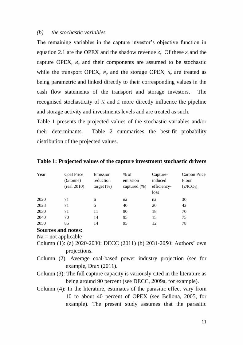
(b) the stochastic variables

The remaining variables in the capture investor’s objective function in

equation 2.1 are the OPEX and the shadow revenue Zt. Of these Zt and the

capture OPEX, Bt, and their components are assumed to be stochastic

while the transport OPEX, Nt, and the storage OPEX, St, are treated as

being parametric and linked directly to their corresponding values in the

cash flow statements of the transport and storage investors. The

recognised stochasticity of Nt and St more directly influence the pipeline

and storage activity and investments levels and are treated as such.

Table 1 presents the projected values of the stochastic variables and/or

their determinants. Table 2 summarises the best-fit probability

distribution of the projected values.

Table 1: Projected values of the capture investment stochastic drivers

Year Coal Price

(£/tonne)

(real 2010)

Emission

reduction

target (%)

% of

emission

captured (%)

Capture-

induced

efficiency-

loss

Carbon Price

Floor

(£/tCO2)

2020 71 6 na na 30

2023 71 6 40 20 42

2030 71 11 90 18 70

2040 70 14 95 15 75

2050 85 14 95 12 78

Sources and notes:

Na = not applicable

Column (1): (a) 2020-2030: DECC (2011) (b) 2031-2050: Authors’ own

projections.

Column (2): Average coal-based power industry projection (see for

example, Drax (2011).

Column (3): The full capture capacity is variously cited in the literature as

being around 90 percent (see DECC, 2009a, for example).

Column (4): In the literature, estimates of the parasitic effect vary from

10 to about 40 percent of OPEX (see Bellona, 2005, for

example). The present study assumes that the parasitic

12

effects range from a high of 20% reducing to about 12% due

to LBD effects.

Column (5): The data range is broadly consistent with DECC’s

projections as cited by Mott MacDonald (2010). In DECC’s

central case, the carbon price increases from £16/tCO2 in

2020 to £70/tCO2 in 2030 and £135/tCO2 in 2040, with an

average of £54/tCO2. The modelling follows this trend.

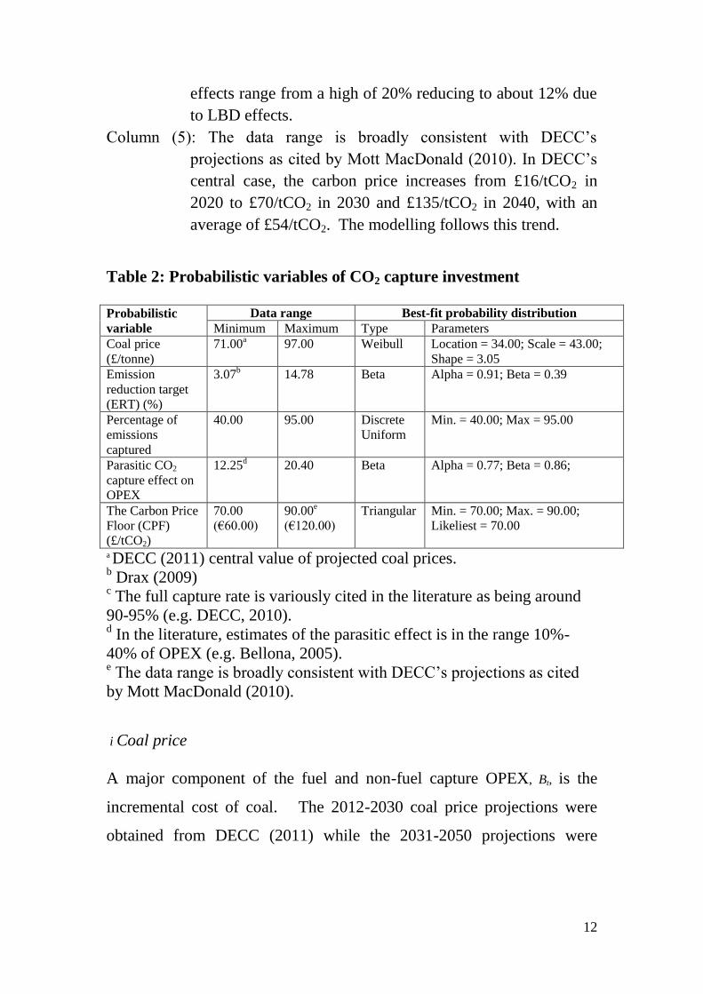
Table 2: Probabilistic variables of CO2 capture investment

Probabilistic

variable

Data range Best-fit probability distribution

Minimum Maximum Type Parameters

Coal price

(£/tonne)

71.00a

97.00 Weibull Location = 34.00; Scale = 43.00;

Shape = 3.05

Emission

reduction target

(ERT) (%)

3.07b

14.78 Beta Alpha = 0.91; Beta = 0.39

Percentage of

emissions

captured

40.00 95.00

Discrete

Uniform

Min. = 40.00; Max = 95.00

Parasitic CO2

capture effect on

OPEX

12.25d

20.40 Beta Alpha = 0.77; Beta = 0.86;

The Carbon Price

Floor (CPF)

(£/tCO2)

70.00

(€60.00)

90.00e

(€120.00)

Triangular Min. = 70.00; Max. = 90.00;

Likeliest = 70.00

a DECC (2011) central value of projected coal prices. b Drax (2009)

c The full capture rate is variously cited in the literature as being around

90-95% (e.g. DECC, 2010). d In the literature, estimates of the parasitic effect is in the range 10%-

40% of OPEX (e.g. Bellona, 2005). e The data range is broadly consistent with DECC’s projections as cited

by Mott MacDonald (2010).

i Coal price

A major component of the fuel and non-fuel capture OPEX, Bt, is the

incremental cost of coal. The 2012-2030 coal price projections were

obtained from DECC (2011) while the 2031-2050 projections were

13

calculated by the authors, based on a stochastic price model5. A summary

of the projected coal prices is presented in Table 1 while the price

forecast methodology is presented in Appendix 1.1. The randomly

generated time path of coal prices in is fitted to a number of probability

distribution curves to determine a best fit for use in the stochastic

optimisation. Using the Anderson-Darling (A-D) probability curve-

fitting criterion in this and all other cases, the best-fitting probability

distribution of the projected coal price was found to be the Weibull

distribution6,7

. This result is presented in Table 2. The cumulative

probability distribution suggests that there is a 60% chance of realising a

real2010 coal price of £75/tonne or less during the forecast period.

ii. Capture-induced plant efficiency loss

CO2 capture substantially adds to a power plant’s investment, energy and

fuel costs. However, there is a general expectation that the experience

gained through learning-by-doing (LBD) will mitigate the costs in the

long-term. In the literature, estimates of the capture-induced parasitic

effect on costs vary from 10% to about 40% of OPEX (see Bellona,

2005). The present study assumes that the effects could range from a

high of 20% reducing to 12% over the study period. This range is close to

the 25%, 18%, 15% and 13% in 2013, 2020, 2028, and 2040 respectively

assumed in DECC (2012c). The projected plant efficiency losses are

presented in Table 1.

5 Unlike the other capture-related model variables with no historic data, the availability of historic data

on coal prices permits the formulation, estimation and forecast of a stochastic price model. 6 The Weibull distribution was the best-fitting under the Chi-square criterion during the period 1993-

2011. 7 The top three best fits are Weibull (0.323), Lognormal (0.334) and Gamma (0.343).

14

In Table 2, the best-fit of the underlying probability distribution of the

forecast is a beta distribution8. The cumulative probability distribution

suggests that there is a 30% chance that the capture-induced loss in plant

efficiency can be reduced from about 20% to about 14% during the study

period.

iii Carbon Price Floor (zt)

In order to reduce risk and encourage low-carbon electricity generation,

the UK Government has introduced a Carbon Price Floor (CPF) that

became operational from April 2013 (HM Treasury, 2010, 2011). The

CPF starts at around £16/tCO2, rising linearly to £30/tCO2 in 2020 and

£70/tCO2 in 2030. No official estimates are available for the period

2031-2050. This study acknowledges that the CPF may fluctuate during

this later period. The official and projected CPFs are presented in Table

1. A triangular probability distribution of the deterministic forecast was

assumed in Table 2. The minimum and maximum CPF values were

respectively assumed to be £70/tonne and £90/tonne with the likeliest

being £70/tonne. The cumulative distribution suggests that there is an

80% chance of the CPF not exceeding £83/tonne between 2031 and 2050.

(iv) Other (physical) influencing variables

The levels of the various costs and revenues discussed thus far depend on

the amount of CO2 captured, Q. However, Q itself is a function of the

capture investor’s emission reduction programme (ERP) and the capture

capacity (CC) at any point in time. That is, Qt = f(ERPt, CCt).

Both ERPt and CCt, are stochastic and affect the investor’s costs and

revenues through their impact on Qt.

8 The A-D top 3 test results are: Beta (0.119), Uniform (0.232) and Weibull (0.318).

15

a. Emission reduction target/programme (ERP)

It is expected that, with increasing CO2 emission mitigation regulations,

UK power plants will undertake ERPs with set performance targets – that

is, emission reduction targets (ERTs). ERTs include the rate at which

renewable fuel sources and co-firing will replace fossil fuels, coupled

with improvements in thermal efficiency through turbine upgrades. Some

coal-fired power plants such as Drax and Longannet (see Drax, 2012 and

ScottishPower, 2009) have recently achieved between 3% and 4%

reduction in their CO2 emission factors through turbine upgrade and co-

firing coal with biomass. Higher and successful ERPs imply less CO2

emissions to capture. Considerable uncertainty surrounds the future level

and pace of ERPs. A summary of the deterministic projected ERT is

presented in Table 1. As shown in Table 2, the best-fit distribution of the

forecast ERT is the beta probability distribution9. The fitted distribution

suggests that there is a 60% chance of achieving up to 15% annual

emissions reduction by generating electricity through co-firing and

turbine upgrades during the study period.

b. Emissions capture capacity (CC)

The emissions capture capacity CC is positively related to Q. The full

capture capacity is variously cited in the literature as being around 90% to

99% of emissions (see DECC, 2012c). This study assumes that the

capture capacity/rate is built up over time, increasing with experience

from about 40% in 2020 to about 95% in 205010

. A summary of the

projected capture rate is presented in Table 1.

9 The top 3 best fits ranked by the Anderson-Darling test criterion are: Beta (3.0), Logistic (3.417), and

Maximum Extreme (3.555). 10

The idea of a progressive roll-out of CO2 capture capacity is consistent with CCSA (2011), and

DECC (2012) who assumed the rate would increase from 85% in 2013 to 90% by 2020.

16

In Table 2, the best-fit probability distribution of the deterministic

forecast is the discrete uniform distribution11

. The cumulative probability

distribution suggests that there is an 80% chance that a capture capacity

of up to 84% of emissions would be attained during the study period.

CO2 storage investment (Oilfield Z)

(a) The decision variables

At the EOR-storage stage, the two decision variables are the level of

CAPEX and the storage fee. Relating to equation (2.2), the CAPEX, Cs0

and s

t are the incremental costs of converting or modifying existing

facilities at the oil field, while the storage fee, p2s, is assumed to be related

to the OPEX. For Field Z the incremental CAPEX for CO2-EOR and

subsequent sequestration is assumed to range between £900 million and

£1.2 billion12

. The unit CO2 storage fee is assumed to range between 10

and 20 percent above the unit field OPEX in the post-EOR period.

(b) The stochastic variables

Using equation (2.2) the key variables whose future time paths are

uncertain are the oil price, s

tp , EOR yield, gt, and the injection (x1t) and

monitoring (αt) cost components of OPEX, Xt. The projected values of

these variables are presented in Table 3 while their best-fit probability

distributions are presented in Table 4.

11

Ranked by the Chi-Square test criterion which was the only one available for the forecast data. The

top 3 best fits are: Discrete Uniform (44.212), Binomial (59.080), and Negative Binomial (68.744). 12

For comparison, the Scottish Centre for Carbon Storage (SCCS) assumed that the CO2-EOR CAPEX

for the following large oilfields in the Central North Sea could be: Claymore £1.1 to £1.2 billion, Scott

£1.2 billion and Buzzard £700 million (SCCS, 2009).

17

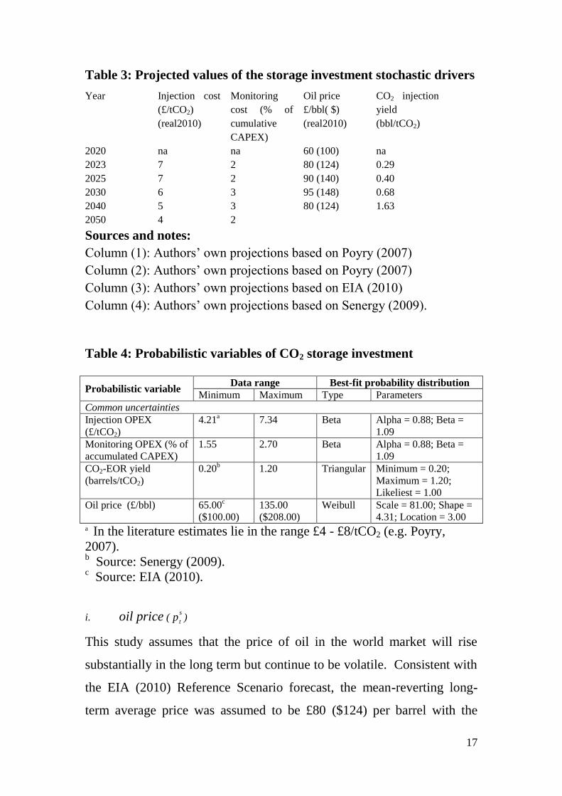
Table 3: Projected values of the storage investment stochastic drivers

Year Injection cost

(£/tCO2)

(real2010)

Monitoring

cost (% of

cumulative

CAPEX)

Oil price

£/bbl( $)

(real2010)

CO2 injection

yield

(bbl/tCO2)

2020 na na 60 (100) na

2023 7 2 80 (124) 0.29

2025 7 2 90 (140) 0.40

2030 6 3 95 (148) 0.68

2040 5 3 80 (124) 1.63

2050 4 2

Sources and notes:

Column (1): Authors’ own projections based on Poyry (2007)

Column (2): Authors’ own projections based on Poyry (2007)

Column (3): Authors’ own projections based on EIA (2010)

Column (4): Authors’ own projections based on Senergy (2009).

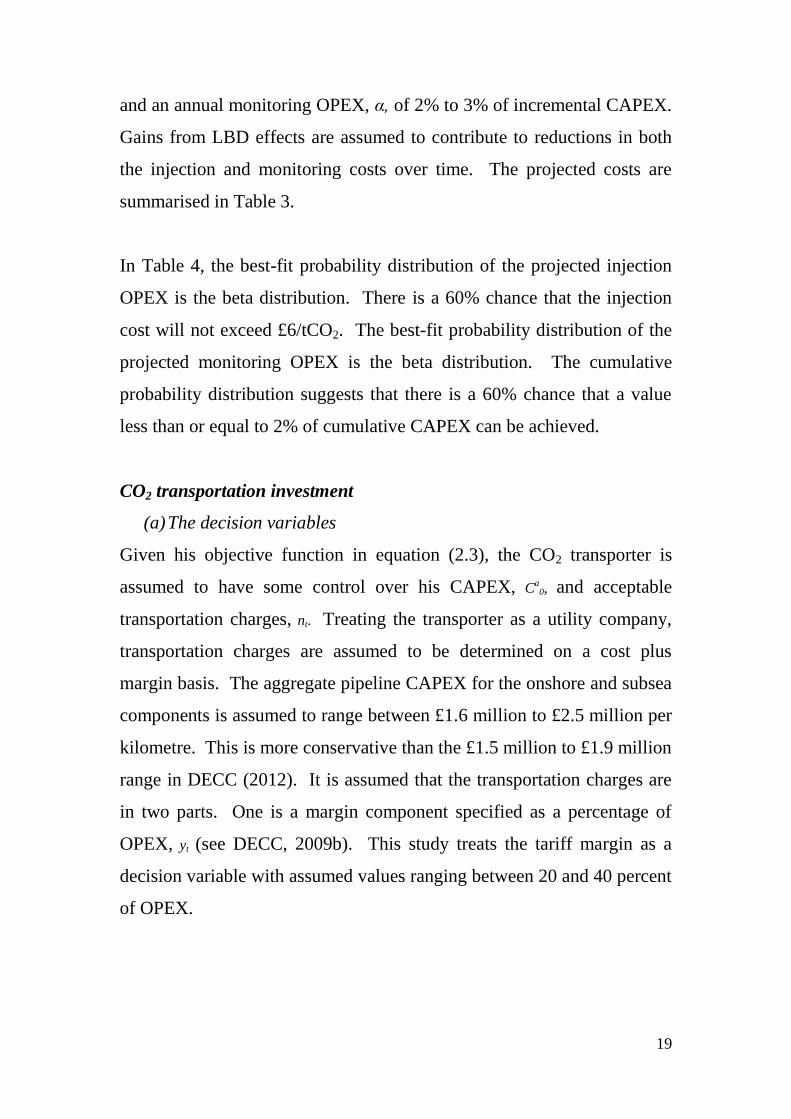
Table 4: Probabilistic variables of CO2 storage investment

Probabilistic variable Data range Best-fit probability distribution

Minimum Maximum Type Parameters

Common uncertainties

Injection OPEX

(£/tCO2)

4.21a

7.34 Beta Alpha = 0.88; Beta =

1.09

Monitoring OPEX (% of

accumulated CAPEX)

1.55 2.70 Beta Alpha = 0.88; Beta =

1.09

CO2-EOR yield

(barrels/tCO2)

0.20b

1.20 Triangular Minimum = 0.20;

Maximum = 1.20;

Likeliest = 1.00

Oil price (£/bbl) 65.00c

($100.00)

135.00

($208.00)

Weibull Scale = 81.00; Shape =

4.31; Location = 3.00 a In the literature estimates lie in the range £4 - £8/tCO2 (e.g. Poyry,

2007). b Source: Senergy (2009).

c Source: EIA (2010).

i. oil price (s

tp )

This study assumes that the price of oil in the world market will rise

substantially in the long term but continue to be volatile. Consistent with

the EIA (2010) Reference Scenario forecast, the mean-reverting long-

term average price was assumed to be £80 ($124) per barrel with the

18

respective lower and upper bounds of £64 ($100) and £106 ($165). The

EIA projections end in 2035. In order to project oil prices beyond that

date, this study used the same mean-reverting commodity price model as

for coal, using a mean-reversion speed of 50% per annum and volatility

of 25%. As shown in Table 4, the best-fit probability distribution of the

projected oil price was found to be the Weibull distribution. There is a

60% chance that the real oil price will reach £80 per barrel or more

during the study period.

ii. CO2-EOR yield (gt)

Considerable uncertainties exist about the CO2 –EOR yield. Estimates in

the literature range from 1 to 4 barrels per tonne of CO2 injected. Bellona

(2005) and Tzimas et al. (2005) in separate studies assumed 3 barrels per

tonne of CO2 injected13

. This study uses a more conservative yield

estimate based on a report by Senergy for the SCCS (2009). This

increases from 0.20 to 1.20 barrels of oil per tonne of CO2 injected,

before diminishing returns set in about halfway through the EOR phase.

The projected EOR yields are presented in Table 3.

In Table 4, the best-fit probability distribution is seen to be triangular

with the likeliest yield of 1 barrel of oil per tonne of CO2 injected. There

is a 60% chance that up to one barrel of oil per tonne of CO2 injected can

be produced during the study period.

iii injection and monitoring OPEX (x1t and α)

Various estimates of the cost per unit of CO2 injected, x1t, exist in the

literature (see Poyry (2007), for example). Based on these this study

assumes an annual injection OPEX of £4 to £7 per tonne of CO2 injected

13

See, also, USA Department of Energy (2006).

19

and an annual monitoring OPEX, α, of 2% to 3% of incremental CAPEX.

Gains from LBD effects are assumed to contribute to reductions in both

the injection and monitoring costs over time. The projected costs are

summarised in Table 3.

In Table 4, the best-fit probability distribution of the projected injection

OPEX is the beta distribution. There is a 60% chance that the injection

cost will not exceed £6/tCO2. The best-fit probability distribution of the

projected monitoring OPEX is the beta distribution. The cumulative

probability distribution suggests that there is a 60% chance that a value

less than or equal to 2% of cumulative CAPEX can be achieved.

CO2 transportation investment

(a) The decision variables

Given his objective function in equation (2.3), the CO2 transporter is

assumed to have some control over his CAPEX, Ca0, and acceptable

transportation charges, nt. Treating the transporter as a utility company,

transportation charges are assumed to be determined on a cost plus

margin basis. The aggregate pipeline CAPEX for the onshore and subsea

components is assumed to range between £1.6 million to £2.5 million per

kilometre. This is more conservative than the £1.5 million to £1.9 million

range in DECC (2012). It is assumed that the transportation charges are

in two parts. One is a margin component specified as a percentage of

OPEX, yt (see DECC, 2009b). This study treats the tariff margin as a

decision variable with assumed values ranging between 20 and 40 percent

of OPEX.

20

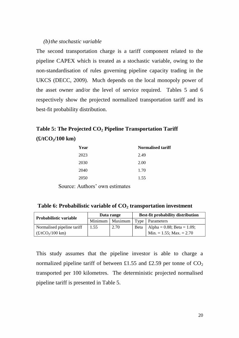
(b) the stochastic variable

The second transportation charge is a tariff component related to the

pipeline CAPEX which is treated as a stochastic variable, owing to the

non-standardisation of rules governing pipeline capacity trading in the

UKCS (DECC, 2009). Much depends on the local monopoly power of

the asset owner and/or the level of service required. Tables 5 and 6

respectively show the projected normalized transportation tariff and its

best-fit probability distribution.

Table 5: The Projected CO2 Pipeline Transportation Tariff

(£/tCO2/100 km)

Year Normalised tariff

2023 2.49

2030 2.00

2040 1.70

2050 1.55

Source: Authors’ own estimates

Table 6: Probabilistic variable of CO2 transportation investment

Probabilistic variable Data range Best-fit probability distribution

Minimum Maximum Type Parameters

Normalised pipeline tariff

(£/tCO2/100 km)

1.55

2.70 Beta Alpha = 0.88; Beta = 1.09;

Min. = 1.55; Max. = 2.70

This study assumes that the pipeline investor is able to charge a

normalized pipeline tariff of between £1.55 and £2.59 per tonne of CO2

transported per 100 kilometres. The deterministic projected normalised

pipeline tariff is presented in Table 5.

21

Table 6 indicates that the best-fit probability distribution of the projected

normalised pipeline tariff is the beta distribution. There is a 60% chance

of a normalised pipeline tariff of £2.15 or more during the study period.

4. Model optimisation, results and discussion

In order to investigate the CCS investors’ positions, the model in Section

2 was optimised from the respective perspectives of the capture and

storage investors, with the transporter being treated as a utility. The

numerical optimisation runs were performed with Crystal Ball, with each

run consisting of 1000 Monte Carlo simulations and 1500 trials per

simulation. Optimal results were obtained for High- and Medium Emitter

scenarios but only the latter are presented and discussed below14

.

The returns to the CCS investors under two alternative investment

climates are shown in Figures 1 to 6.

i. Returns to the capture investment under two investment

scenarios.

Fig. 1: The NPV of the capture investment (£ million, 2010) (Plant B)

14

The interested reader may obtain the High-Emitter results from the corresponding author. The High-

Emitter case assumes the involvement in the CCS value chain of a high CO2-emitting PCSCFGD

power plant with annual emissions of between 18 and 21 MtCO2/year.

0

0.01

0.02

0.03

0.04

0.05

0.06

0

10

20

30

40

50

60

70

80

90

754 787 819 851 883 912

pro

ba

bil

ity

fre

qu

en

cy

£ million

Source B-to-Sink Z CCS investment: Capture investment NPV under capture-friendly conditions

22

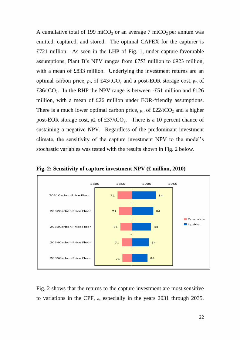
A cumulative total of 199 mtCO2 or an average 7 mtCO2 per annum was

emitted, captured, and stored. The optimal CAPEX for the capturer is

£721 million. As seen in the LHP of Fig. 1, under capture-favourable

assumptions, Plant B’s NPV ranges from £753 million to £923 million,

with a mean of £833 million. Underlying the investment returns are an

optimal carbon price, p1, of £43/tCO2 and a post-EOR storage cost, p2, of

£36/tCO2. In the RHP the NPV range is between -£51 million and £126

million, with a mean of £26 million under EOR-friendly assumptions.

There is a much lower optimal carbon price, p1, of £22/tCO2 and a higher

post-EOR storage cost, p2, of £37/tCO2. There is a 10 percent chance of

sustaining a negative NPV. Regardless of the predominant investment

climate, the sensitivity of the capture investment NPV to the model’s

stochastic variables was tested with the results shown in Fig. 2 below.

Fig. 2: Sensitivity of capture investment NPV (£ million, 2010)

Fig. 2 shows that the returns to the capture investment are most sensitive

to variations in the CPF, zt, especially in the years 2031 through 2035.

71

71

71

71

71

84

84

84

84

84

£800 £850 £900 £950

2031Carbon Price Floor

2032Carbon Price Floor

2033Carbon Price Floor

2034Carbon Price Floor

2035Carbon Price Floor

Fig.__: Sensitivity of Capture investment NPV

Downside

Upside

23

The two CPF prices to which the capture investment NPV is most

sensitive are £71/tCO2 and £84/tCO2. The latter is the upside of the

variable while the former is the downside.

ii. Returns to the EOR investment under two investment scenarios.

Fig. 3: The NPV of CO2-EOR investment (£ million) (real2010) (Field Z)

The optimal CO2-EOR investment in both scenarios was determined as

£901 million. The total EOR is 131 mmbbls. Under the capture-

favourable conditions in the LHP of Fig. 3, the NPV ranges from £4

million to £617 million with a mean of £298 million. The optimal oil

price,s

tp , during the EOR-phase is £110/bbl, while the optimal post-EOR

storage fee, p2s, received is £36/tCO2. Under EOR-favourable conditions

the minimum investment return is £229 million, with a maximum of £816

million and a mean of £484 million. Much of the improvement in this

scenario emanates from the substantial reduction in the CO2 cost from, p1s,

£43/tCO2 to £22/tCO2 and the higher storage fee, p2s, of £37/tCO2.

Both the coefficient of variability (not shown) and NPV range are

significantly greater in the RHP than the LHP, underlining the point that

even under more favourable conditions, returns to EOR investment

0

0.01

0.02

0.03

0.04

0.05

0.06

0

10

20

30

40

50

60

70

80

47 151 256 361 466 560

pro

bab

ility

fre

qu

en

cy

£ million

Source B-to-Sink Z CCS investment: Storage investment NPV under capture-friendly conditions

24

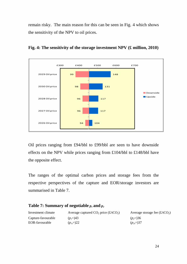
remain risky. The main reason for this can be seen in Fig. 4 which shows

the sensitivity of the NPV to oil prices.

Fig. 4: The sensitivity of the storage investment NPV (£ million, 2010)

Oil prices ranging from £94/bbl to £99/bbl are seen to have downside

effects on the NPV while prices ranging from £104/bbl to £148/bbl have

the opposite effect.

The ranges of the optimal carbon prices and storage fees from the

respective perspectives of the capture and EOR/storage investors are

summarised in Table 7.

Table 7: Summary of negotiable p1 and p2

Investment climate Average captured CO2 price (£/tCO2) Average storage fee (£/tCO2)

Capture-favourable (p1=)43 (p2=)36

EOR-favourable (p1s=)22 (p2s=)37

99

98

96

96

94

148

131

117

117

104

£300 £400 £500 £600 £700

2029 Oil price

2030 Oil price

2028 Oil price

2027 Oil price

2026 Oil price

Fig. __: Sensitivity of Storage investment (oil price in £/bbl)

Downside

Upside

25

iii. Returns to the transport investment under two investment

scenarios

Fig. 5: The NPV of transport investment (£ million, 2010)

The optimal transport investment was determined as being £602 million.

The differences in the capture- and EOR-friendly conditions make little

difference to the profitability of the CO2 transport investment. Fig. 5

shows that the returns are virtually the same in both scenarios, consistent

with the utility-type investment. The NPV ranges from £4 million to £81

million with a mean value of £40 million.

0

0.01

0.02

0.03

0.04

0.05

0.06

0

10

20

30

40

50

60

70

80

90

10 22 35 47 60 71

pro

bab

ility

fre

qu

en

cy

£ million

Source B-to-Sink Z CCS investment: Transport investment NPV under capture-friendly conditions

26

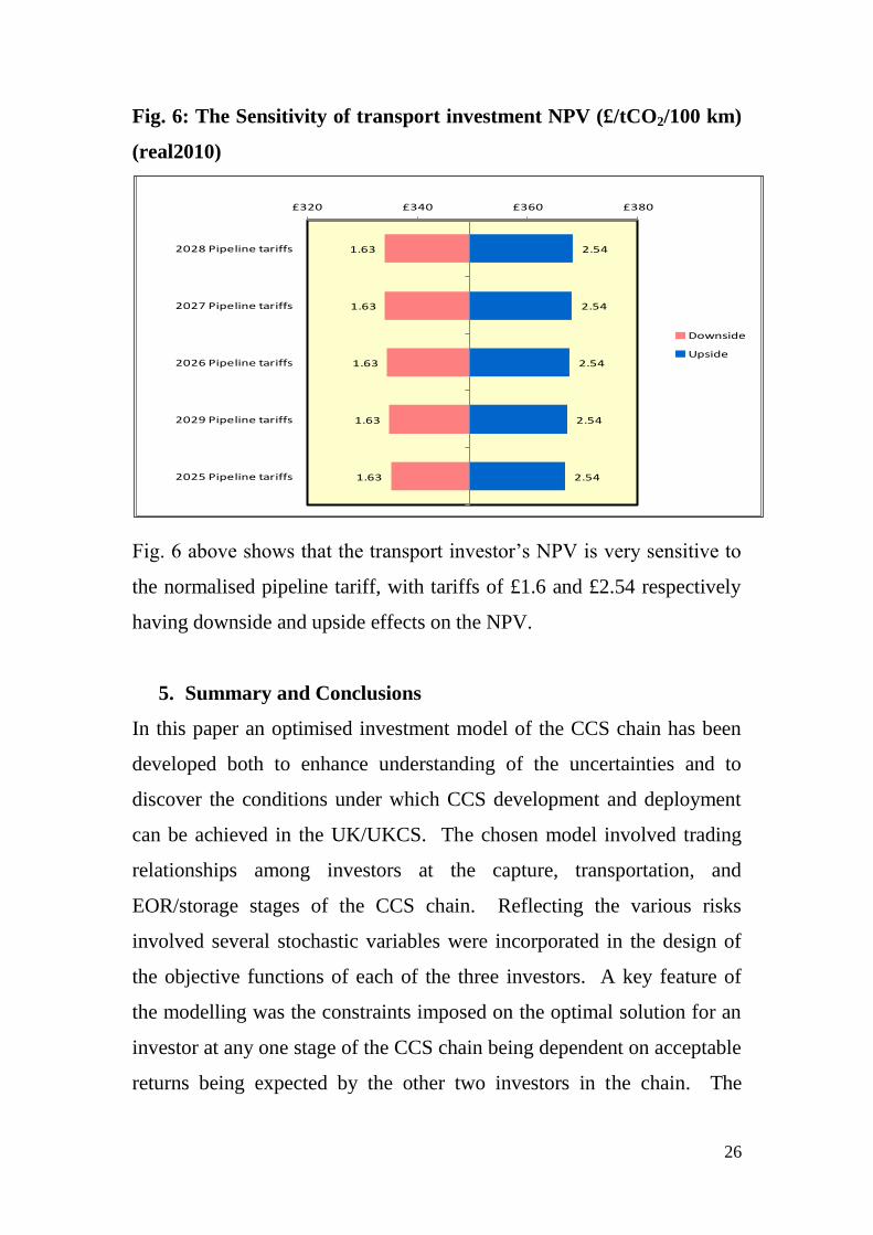
Fig. 6: The Sensitivity of transport investment NPV (£/tCO2/100 km)

(real2010)

Fig. 6 above shows that the transport investor’s NPV is very sensitive to

the normalised pipeline tariff, with tariffs of £1.6 and £2.54 respectively

having downside and upside effects on the NPV.

5. Summary and Conclusions

In this paper an optimised investment model of the CCS chain has been

developed both to enhance understanding of the uncertainties and to

discover the conditions under which CCS development and deployment

can be achieved in the UK/UKCS. The chosen model involved trading

relationships among investors at the capture, transportation, and

EOR/storage stages of the CCS chain. Reflecting the various risks

involved several stochastic variables were incorporated in the design of

the objective functions of each of the three investors. A key feature of

the modelling was the constraints imposed on the optimal solution for an

investor at any one stage of the CCS chain being dependent on acceptable

returns being expected by the other two investors in the chain. The

1.63

1.63

1.63

1.63

1.63

2.54

2.54

2.54

2.54

2.54

£320 £340 £360 £380

2028 Pipeline tariffs

2027 Pipeline tariffs

2026 Pipeline tariffs

2029 Pipeline tariffs

2025 Pipeline tariffs

Fig. __: Sensitivity of Transport investment (tariffs are normalised)

Downside

Upside

27

modelling produced further insights into the nature of the problem by

finding the optimal investment of each participant in the chain. A

consequence of this procedure was that two values for the optimal CO2

prices and storage fees were found, reflecting the separate perspectives of

the capture and EOR/ storage investors. In the case of the Plant B the

investor has an optimal asking CO2 price of £43/tCO2 while the storer’s

optimal offer price is £22/tCO2. With respect to the EOR-storage fee the

corresponding optimal values are an offer price of £36/tCO2 from the

capture investor’s perspective and an asking price of £37/tCO2 from the

storer’s viewpoint. Reflecting the mutual interdependence of the

integrated CCS investments, while attempting to avert the tragedy of the

anticommons (Parente, 2012), the parties can negotiate and reach a

satisfactory agreement on the prices that would offer acceptable returns to

their individual investments. The price differentials show the scope for

negotiation between the two parties, with any value within the range

ensuring that the overall chain of investments remains viable. The

uncertainties and boundaries for negotiation among the parties can be

reduced by the wider provision and sharing of the maximum amount of

information on the likely costs of the various elements in the CCS chain,

paving the way towards co-operative Nash equilibrium contractual terms.

Both the broad range of prices of oil (£110/bbl to £114/bbl) and the

traded CO2 (£22/tCO2 to £43/tCO2) required to ensure the optimality of

the model solutions may appear rather high. It should be noted, however,

that the long-term oil price range is consistent with other studies

including EIA (2010)15

. Also, the CO2 prices are consistent with those

planned for the CPF. The CPF mechanism involves the extension of the

15

SCCS (2009) suggests that oil prices above $100/bbl would be required to kick-start some CO2-EOR

projects in the UKCS.

28

Climate Change Levy (CCL) to fossil fuels used for power generation16

.

The results of this study are useful in quantifying the level of price

support that may be required. Currently, EOR in the UKCS is fully

subject to the North Sea oil taxation regime which entails tax at an overall

rate of 81% on profits from fields developed before March 1993, and a

rate of 62% on profits from fields developed after that date.

Disincentives to EOR schemes can readily emerge, and tax reliefs for

EOR projects could enhance investment incentives. For example, the

new Brownfield Allowance could readily be extended to apply to CO2

EOR projects.

16

Government revenue from CPF is projected to reach £1.4 billion as early as 2015-2016 (HM

Treasury, 2011).

29

REFERENCES

Abadie, L.M., and Chamorro, J.M. (2008). “European CO2 prices and

Carbon Capture Investments.” Energy Economics 30, 2992-3015.

Bachu, S. (2004). “Evaluation of CO2 Sequestration Capacity in Oil and

Gas reservoirs in the Western Canada Sedimentary Basin.” Alberta

Energy Research Institute, Canada.

Bellona Foundation (2005). CO2 for EOR on the Norwegian Shelf – A

Case Study. Bellona Report August 2005, Norway.

Carbon Capture and Storage Association (CCSA) (2011). A Strategy for

CCS in the UK and Beyond, Report available online

http://www.ccsassociation.org/press-centre/reports-and-publications/

Department of Energy and Climate Change (DECC) (2009a). A

Framework for Developing Clean Coal, London, United Kingdom.

Department of Energy and Climate Change (DECC) (2009b).

Developing a Regulatory Framework for CCS Transportation

Infrastructure, prepared for DECC by NERA Consulting, London, United

Kingdom.

Department of Energy and Climate Change (DECC) (2011). DECC Coal

Price Projections, London, United Kingdom.

Department of Energy and Climate Change (DECC) (2012a). Energy Bill

2012-13: Emissions Performance Standard, London, United Kingdom.

Department of Energy and Climate Change (DECC) (2012b). PILOT

Summit Workstream, 23rd

May 2012, Aberdeen, United Kingdom.

Department of Energy and Climate Change (DECC) (2012c). The

Potential for Reducing the Costs of CCS in the UK, Interim Report,

November 2012, London, United Kingdom.

http://www.decc.gov.uk/assets/decc/11/cutting-emissions/carbon-capture-

storage/6987-the-potential-for-reducing-the-costs-of-cc-in-the-.pdf

Drax Group PLC. (2012). Inside Drax, Annual Report and Accounts

2011, Selby, Yorkshire, United Kingdom.

30

HM Treasury (2010). Carbon Price Floor: Support and Certainty for

Low-carbon Investment, London, United Kingdom.

HM Treasury (2011). Budget 2011, London, United Kingdom.

Ho, M.T., Allinson, G.W., Wiley, D.E. (2011). Comparison of MEA

Capture Cost for Low CO2 Emissions Sources in Australia. International

Journal of Greenhouse Gas Control, 5, 49-60.

Kemp, A.G., and Kasim, A.S. (2010). “A Futuristic Least-cost

Optimisation Model of CO2 Transportation and Storage in the UK/UK

Continental Shelf.” Energy Policy, 38, 3652-3667.

Kettunen, J., Bunn, D.W., and Blyth, W. (2011). “Investment

Propensities under Carbon Price Uncertainty.” The Energy Journal 32(1):

77-117.

Klokk, Ø., Schreiner, P.F., Pages-Bernaus, A., Tomasgard, A. (2010).

“Optimizing a CO2 value Chain for the Norwegian Continental Shelf.”

Energy Policy, 38, 6604-6614.

Liang, Xi, Li, Jia (2012). “Assessing the Value of Retrofitting Cement

Plants for Carbon Capture: A Case Study of a Cement Plant in

Guangdong, China, Energy Conversion and Management.” 64, 454-465.

Mott MacDonald (2010). UK Electricity Generation Costs Update,

Brighton, United Kingdom.

Parente, M.D. and Winn, A.M. (2012). “Bargaining Behavior and the

Tragedy of the Anticommons.” Journal of Economic Behavior &

Organization 84: 475-490.

Poyry Energy Consulting (2007). Analysis of Carbon Capture and

Storage Cost-Supply Curves for the UK. Economic Analysis of Carbon

Capture and Storage in the UK, London

Rubin, E.S., Yeh, S., Antes, M., Berkenpas, M., Davison, J. (2007). Use

of Experience Curves to Estimate the Future Cost of Power plants with

CO2 Capture. International Journal of Greenhouse Gas Control, 1, pp

188-197.

31

Scottish Centre for Carbon Storage (SCCS) (2009). Opportunities for

CO2 Storage Around Scotland – an Integrated Strategic Research Study.

SCCS Report available online: www.erp.ac.uk/sccs

ScottishPower (2009). CSR Annual Review 2008, Glasgow, United

Kingdom

Senergy (2009). Response and Comments on the SCCS 2009 Report,

Aberdeen, United Kingdom.

Tzimas, E., Georgakaki, A., Garcia Cortes, C., and Peteves (2005).

Enhanced Oil Recovery Using Carbon Dioxide in the European Energy

System. Institute for Energy, Petten, The Netherlands.

USA Department of Energy (2006). Evaluating The Potential for

“Game-Changer” Improvements in Oil Recovery Efficiency from CO2

Enhanced Oil Recovery. Washington.

USA Department of Energy/Energy Information Administration (EIA)

(2010). Annual Energy Outlook 2010, With Projections to 2035, April

2010, Washington

Yeh, S. and Rubin, E.S. (2007). “A Centurial History of Technological

Change and Learning Curves for Pulverized Coal-fired Utility Boilers.”

Energy, 32: 1996-2005.

32

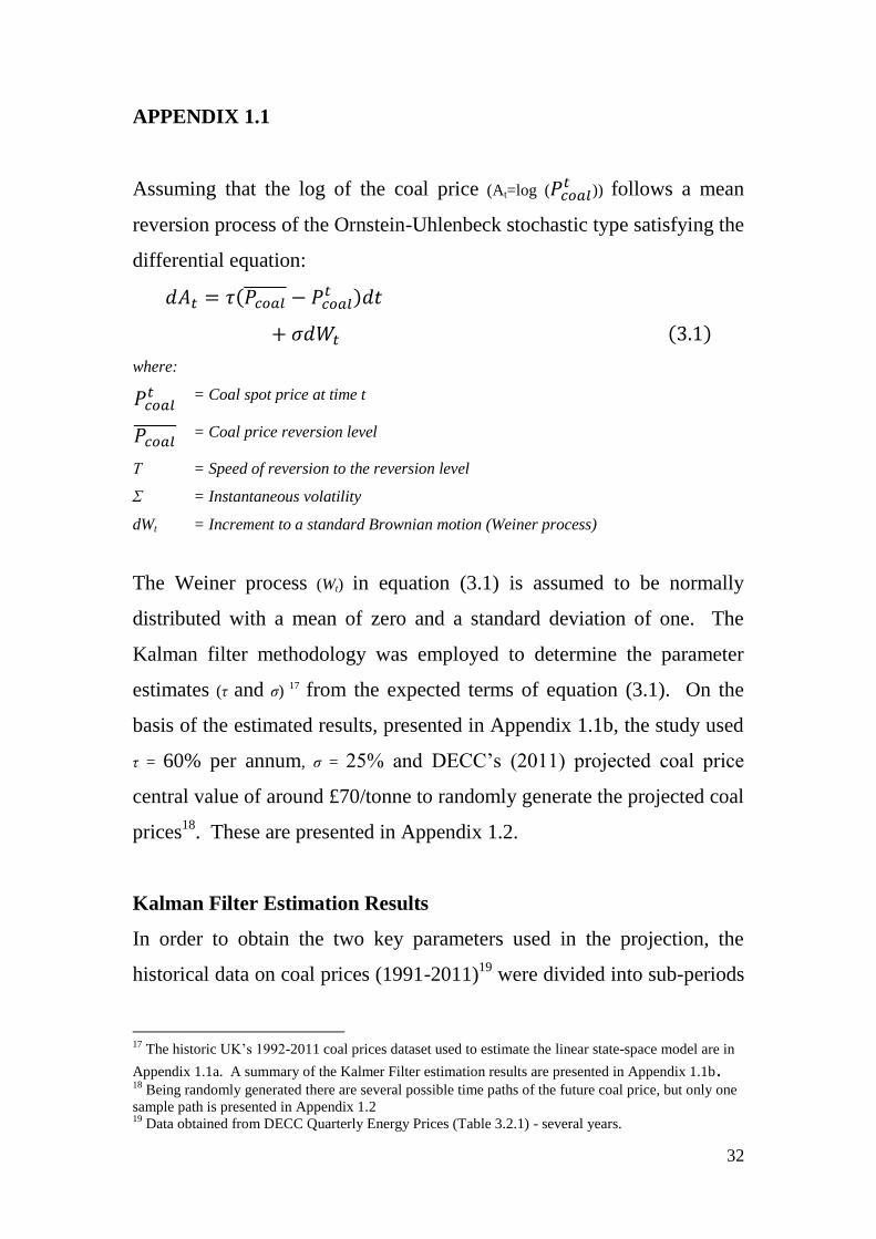
APPENDIX 1.1

Assuming that the log of the coal price (At=log (

)) follows a mean

reversion process of the Ornstein-Uhlenbeck stochastic type satisfying the

differential equation:

where:

= Coal spot price at time t

= Coal price reversion level

Τ = Speed of reversion to the reversion level

Σ = Instantaneous volatility

dWt = Increment to a standard Brownian motion (Weiner process)

The Weiner process (Wt) in equation (3.1) is assumed to be normally

distributed with a mean of zero and a standard deviation of one. The

Kalman filter methodology was employed to determine the parameter

estimates (τ and σ) 17

from the expected terms of equation (3.1). On the

basis of the estimated results, presented in Appendix 1.1b, the study used

τ = 60% per annum, σ = 25% and DECC’s (2011) projected coal price

central value of around £70/tonne to randomly generate the projected coal

prices18

. These are presented in Appendix 1.2.

Kalman Filter Estimation Results

In order to obtain the two key parameters used in the projection, the

historical data on coal prices (1991-2011)19

were divided into sub-periods

17

The historic UK’s 1992-2011 coal prices dataset used to estimate the linear state-space model are in

Appendix 1.1a. A summary of the Kalmer Filter estimation results are presented in Appendix 1.1b. 18

Being randomly generated there are several possible time paths of the future coal price, but only one

sample path is presented in Appendix 1.2 19

Data obtained from DECC Quarterly Energy Prices (Table 3.2.1) - several years.

33

to get a clearer picture of a trend. By segmenting the dataset into sub-

periods (for example, 1996-2011, 2000-2011 etc.) the estimated linear

state-space model yielded (in the EViews econometric package used for

the purpose) the following results:

period volatility (σ) reversion

speed (τ)

log likelihood probability of rejection

volatility reversion

speed

1991-2011 0.138 0.999 7.363 0.000 0.000

2000-2011 0.164 0.997 1.921 0.000 0.000

2003-2011 0.187 0.797 1.823 0.000 0.115

2004-2011 0.193 0.670 1.513 0.000 0.267

2005-2011 0.189 0.440 1.609 0.005 0.486

2006-2011 0.174 0.232 1.945 0.006 0.669

In summary, the estimated price volatility (σ) and mean-reversion (τ)

speed parameters lie in the following ranges:

14 %< σ<20%

23 %< τ<90%