an optimization-based approach to understanding sensory
TRANSCRIPT

An Optimization-Based Approach to Understanding Sensory Systems
Daniel Yamins∗
Nothing in biology makes sense except in light of evolution.
— Theodosius Dobzhansky
Nothing in neurobiology makes sense except in light of behavior.
— Gordon Shepherd
Abstract Recent results have shown that deep neural networks (DNN) may have significant potential toserve as quantitatively precise models of sensory cortex neural populations. However, the implications theseresults have for our conceptual understanding of neural mechanisms are subtle. This is because many modernDNN brain models are best understood as the products of task-constrained optimization processes, unlike theintuitively simpler hand-crafted models from earlier approaches. In this chapter, we illustrate these issues byfirst discussing the nature of information processing in the primate ventral visual pathway, and review resultscomparing the response properties of units in goal-optimized DNN models to neural responses found throughoutthe ventral pathway. We then show how DNN visual system models are just one instance of a more generaloptimization framework whose logic may be applicable to understanding the underlying constraints that shapeneural mechanisms throughout the brain.
An important part of a scientist’s job is to answer “why” questions. For cognitive neuroscientists, a coreobjective is to uncover the underlying reasons why the structures of the human brain are as they are. Sincebrains are biological systems, answering such questions is ultimately a matter of identifying the evolutionary anddevelopmental constraints that shape brain structure and function. Such constraints are in part architectural:what large-scale brain structures are put in place genetically to help a brain help its host organism bettermeet evolutionary challenges? In light of the centrality of behavior in understanding the brain, an ethologicalinvestigation is also indicated: what behavioral goals most strongly constrain a given neural system? And sincemany complex behaviors in higher organisms are not entirely genetically determined and must instead be partlyderived through experience of the world, a core question of learning is also involved: how do learning rules thatabsorb experiential data constrain what brains look like?
The interactions between architectural structure, behavioral goals, and learning rules suggest a quantita-tive optimization framework as one route toward answering these “why” questions. Put simply, this means:postulating one or several goal behavior(s) as driving the evolution and/or development of a neural system ofinterest; finding architecturally plausible computational models that (attempt to) optimize for the behavior;and then quantitatively comparing the internal structures arrived at in the optimized models to measurementsfrom large-scale neuroscience experiments. To the extent that there is a match between optimized models andthe real data that is very substantially better than that found for various controls (e.g. models designed byhand or optimized for other tasks), this is evidence that something important has been understood about theunderlying constraints that shape the brain system under investigation. Though it might sound challenging toput this approach into practice, recent successes suggest we might add to our list of maxims the observationthat nothing in computational cognitive neuroscience makes sense except in light of optimization.
Case Study: The Primate Ventral Visual StreamThe most thoroughly developed example of these optimization-based ideas is the visual system — and inparticular, the ventral visual stream in humans and non-human primates. While a complete review of the workthat lead to the present understanding of the primate ventral stream is beyond the scope of this chapter (seeDiCarlo et al. 1 for a summary), discussing key computational aspects of the ventral stream in some detail willlay the groundwork for the optimization approach more generally.
∗Departments of Psychology and Computer Science, and the Stanford Neurosciences Institute, Stanford University;[email protected]

The computational crux of the vision problem. The human brain effortlessly reformats the “blooming,buzzing confusion” of unstructured visual datastreams into powerful abstractions that serve high-level behavioralgoals such as scene understanding, navigation, and action planning2. But parsing retinal input into rich object-centric scene descriptions is a major computational challenge. The crux of the problem is that the axes of thelow-level input space (i.e. light intensities at each retinal “pixel”) don’t correspond to the natural axes alongwhich high-level constructs vary. For example, translation, rotation in depth, deformation, or re-lighting of asingle object (e.g. one person’s face) can lead to large and complex non-linear transformations of the originalimage. Conversely, images of two ecologically quite distinct objects, e.g. different individuals’ faces, may be veryclose in pixel space. Behaviorally-relevant dimensions are thus highly “tangled” in the original input space3, andto recognize objects and understand scenes the brain must accomplish a complex and often ill-posed non-linearuntangling process rapidly and accurately1.
Hierarchy and Retinotopy in the Ventral Pathway Sparked by the seminal ideas of Hubel and Wiesel,six decades of work in systems neuroscience have shown that the homologous visual system in humans and non-human primates generates robust object recognition behavior via a series of anatomically-distinguishable corticalareas known as the ventral visual stream (Fig. 1a-b)1,4–7. Two basic principles of architectural organizationemerging from this work are that the ventral stream is:
1. hierarchical, with visual information passing along a cascade of processing stages embodied by the distinctcortical areas, and
2. retinotopic, composed of structurally similar operations with spatially local receptive fields tiling the overallvisual field, with decreasing spatial resolution in each subsequent stage of the hierarchy.
Visual areas early in the hierarchy, such as V1 cortex, capture low-level features including edges and center-surround patterns8,9. Neural population responses in the highest ventral visual area, anterior inferior temporal(AIT) cortex, can be used to decode object category, robust to significant variations present in natural im-ages10–12. Mid-level visual areas such as V2, V3, V4 and posterior IT (PIT) are less well-characterized bysuch “word models” than higher or lower visual areas closer to the sensorimotor periphery. Nonetheless, theseintermediate areas appear to contain computations at an intermediate level of complexity between simple edgesand complex objects, along a pipeline of increasing receptive field size1,13–20
Linear-Nonlinear Cascades. A core hypothesis is that ventral stream employs sensory cascades because:(i) the overall stimulus-to-neuron transforms required to support complex behaviors are extremely complicated— after all, since the original input tangling is highly non-linear, the inverse untangling process is also highlynon-linear; but (ii) the capacities of any single stage of neural processing are limited to comparatively simpleoperations such as weighted sums of inputs, thresholding nonlinearities, and local normalization8. To buildup a sufficiently complex end-to-end transform with a reasonable number of neurons, a cascade of stages isneeded. Complex non-linear transformations arise from multiple such stages applied in series21. Such cascadesare present not just in the visual system but are common in a wide variety of sensory areas22–25.
A very simplified version of the feedforward component of the multi-stage sensory cascade may thus berepresented symbolically by:
stimulusT17−→ n1
T27−→ n2 . . .Ttop7−→ ntop (1)
where the ni represent neural responses in brain area i, and Ti is the transform computed by the neurons in areai based on input from area i− 1. In the macaque ventral stream this will (at least) include several subcorticalstages prior to the ventral stream (e.g. the retinal ganglion and LGN), followed by cortical areas V1, V2, V4,PIT, and AIT. The homologous structure in humans is similar but likely to be substantially more complex26.
Robust empirical observations8 suggest that the transforms Ti can be reasonably well-modeled as Linear-Nonlinear (LN) blocks of the form:
Ti = Ni ◦ Li.
Biologically, the linear transforms Li are inspired by the observation that neurons are admirably suited for takingdot-products, i.e. summing up their inputs on each incoming dendrite, weighted by synaptic strengths. Thetransforms Li formalize the synaptic strengths as numerical matrices. Mathematically, the Li map the inputfeature space output by one area to an intermediate feature space in the next. In the case of L1 (the transform
2

LN
LN
...
LN
LN
...
...
Spatial Convolutionover Image Input ...
Φ1
Φ2
Φk
⊗⊗
⊗Filter Threshold Pool Normalize
Operations in Linear-Nonlinear Layer
...
LN
LN
LN
LN
LN
LN
LN
...
DOG
pixels
RGC LGN
V1 V2
V4 PIT
T(•) PITV2
V4
Rapid VisualPresentation
V1
CITAIT
CIT AIT
?? ?
b)
c)
CategoryLocationSizePose
. . .
D1D2D3D4Dn
Stimulus Neurons Behaviora) decodingencoding
Figure 1: Hierarchical Convolutional Neural Networks As Models of Sensory Cortex. (a.) The basic frameworkin which sensory cortex is studied is one of encoding, the process by which stimuli are transformed into patterns of neuralactivity, and decoding, the process by which neural activity generates behavior. (b.) The ventral visual pathway of humansand non-human primates is one of the most comprehensively studied sensory systems in neuroscience. It consists of aseries of connected cortical brain areas that are thought to operate in a sensory cascade, from early visual areas such asV1, to later visual areas such as inferior temporal (IT) cortex. Neural responses in the ventral pathway are believed toencode an abstract representation of objects in visual images. (c.) Hierarchical Convolutional Neural Networks (HCNNs)are multilayer neural networks that have been proposed as models of the ventral pathway. Each layers of an HCNN is madeup of a Linear-Nonlinear (LN) combination of simple operations such as filtering, thresholding, pooling, and normalization.The filterbank in each layer consists of a set of weights analogous to synaptic strengths. Each filter in the filter bankcorresponds to a distinct template, analogous to gabor wavelets with different frequencies and orientations (the imageshows a model with four filters in layer 1, 8 in layer two, and so on). The operations within a layer are applied locally tospatial patches within the input, corresponding to simple, limited-size receptive fields (the red boxes in the figure). Thecomposition of multiple layers leads to a complex nonlinear transform of the original input stimulus. At each layer, retinopydecreases and effective receptive field size increases.
between the input image and the first visual area, taken to be either subcortical or in V1), the input space isthe three-channel RGB-like representation of pixels, while the output space is substantially higher-dimensional,corresponding to number of different neural projections computed at each retinotopic location. An extensiveline of research characterizing V1 responses8,27,28 yielded the realization that the linear transforms early on thein cascade can be reasonable well-characterized as spatial convolution with a filterbank of Gabor wavelets in arange of frequencies and orientations29.
The nonlinear component Ni has been shown to involve combinations of very basic transforms, includingrectification, pooling, and normalization operations8,19. While the Ti’s are simple, it is critical that they are atleast somewhat nonlinear: the composition of linear operations is linear, so additional complexity can’t be builtup by a sequence of linear operations, and there would be no evolutionary point to allocating multiple brainareas for them in the first place.
It is tempting to ascribe specific functional roles for each of the constituent operations within an LN block,described in terms of features of the original input stimulus. While this may be possible early in the sensorycascade, the compounding of multiple nonlinearities makes it unlikely that this type of description is adequate forintermediate or higher sensory areas. Instead, it is probably more effective to think of the LN block as combininga dimension-expanding component (the linear filtering step), a dimension-reducing aggregation component (thepooling operation), and a range-centering component to ensure that the cascade can be effectively extendedhierarchically (the normalization operations). These features allow LN cascades to cover a wide range of complexnonlinear functions in an efficient manner30,31, consistent with the idea that good LN cascade architectures canbe discovered by evolutionary and developmental processes.
A Common Visual Feature Basis. The features computed by the sensory cascade are often thought ofas constituting a visual representation. One way to interpret this idea is that the output from area ntop —
3

which is considerably upstream of highly-task-modulated decision making or motor areas — is able to supportobserved organism output behaviors via simple decoders. Symbolically, this is the observation that the pipelinein diagram (1) can be extended to:
stimulus . . . 7−→ ntopD7−→ behavior (2)
where D is a population decoder. The requirement that D be “simple” just means that it can also be castin the form of a single LN block rather than itself requiring many stages of nonlinearity. In the case of themacaque visual system, the role of ntop seems to be played by anterior IT cortex, where it has been robustlyshown that simple decoders such as linear classifiers or linear regressors operating on neural responses in ITcortex can support patterns of visual behavior at a high degree of behavioral resolution3,6,10,12,32. The linearclassifiers embody a computational description of hypothetical decoding circuits downstream of the ventral visualrepresentation33,34.
The representation concept is enhanced by the observation that IT cortex can provide useful support formany different visual behaviors. In addition to object category, attributes such as fine-grained within-categoryidentification, object position, size, and pose, and complex lighting and material properties, can be decodedfrom IT neural activity35,36. Symbolically, this might be represented by the diagram:
. . . ntop
CategoryLocationSizePose
. . .
stimulusD1D2D3D4Dn
in which D1, D2, . . . are different readout decoders for the various possible visually-driven behaviors.A key observation is that for naturalistic scenes with realistically high levels of image variability, these same
visual properties cannot be robustly read out from the visually-evoked neural responses in earlier areas such asthe retina, V1 or V2 using simple decoders, and only partially in intermediate areas such as V410,35. Of course,the information must in some way be present in these areas since the properties can be determined by lookingat the image. However, as alluded to earlier, these properties are “tangled up” in the representations in earlyareas, and so cannot be easily decoded. The nonlinear operations of the ventral stream cascade culminating inthe IT representation have reformatted the information in the input image stimuli into a common basis fromwhich it is possible to generate many different behaviorally-relevant readouts.
Not Just an Information Channel. These considerations suggest that the ventral stream is not bestthought of as a “channel” in the sense of Shannon information theory. As a result of (converse of) the Shannon’sfamous channel coding theorem, with every step of the cascade, the system can only lose information in aninformation-theoretic sense37. The more stages in the case, the less good it will be as a pure information channel.The existence of a many-stage LN cascade in the ventral pathway suggests that the evolutionary constraint on thesystem is not the veridical preservation of information about the stimulus. Rather, the constraining evolutionarygoal of the sensory cascade is more likely to be making behaviorally-relevant information — such as the identityof a face present in the image — much more explicitly available for easy access by downstream brain areas,while discarding other information about the stimuli — such as pixel-level details — that are less behaviorallyrelevant.
Neural Network Models of the Ventral StreamIn this section, we’ll discuss how the neurophysiological observations described above can be formalized
mathematically. But before diving into models of the ventral stream, it is worth briefly considering why wemight want to make quantitative neural network models of the ventral stream in the first place. After all,neuroscientists did not need such models to discover the important insights described in the previous section.
Two convergent problems, however, strongly motivate the building of large-scale formal models. First,the simpler word-model approach that had been useful for characterizing the shape of visual feature tuningcurves in earlier cortical areas such as the retina or V1 were found to be difficult to generalize to intermediateand higher-level visual areas38. Though some progress has been made using intuition to find visual features
4

to which intermediate and higher-area neurons would respond7,20,39, a more systematic approach is needed toorganize and generalize these disparate observations. Second, it turned out that the most naive implementationsof multi-layer hierarchical retinotopic models performed very poorly on tests of performance generalization inreal-world settings40. Although hierarchy and retinotopy appeared to be important high-level principles, theywere insufficiently detailed to actually produce operational algorithms with anything like the visual abilities of amacaque or a human. Echoing Feynman’s famous dictum that “What I cannot create, I do not understand,”the inability to create from scratch a truly working visual recognition system meant that some key feature ofunderstanding was missing.
Hierarchical Convolutional Neural Networks Hierarchical Convolutional Neural Networks (HCNNs) area broad generalization of Hubel and Wiesel’s ideas that has been developed over the past 40 years by researchersin biologically-inspired computer vision41–43. HCNNs consist of cascades of layers containing simple neural circuitmotifs repeated retinotopically across the sensory input (Fig. 1c). Each layer is simple, but a deep networkcomposed of such layers computes a complex transformation of the input data — roughly analogous to theorganization the ventral stream. The specific operations comprising a single HCNN layer were inspired directlyby the LN neural motif8, including: convolutional filtering, a linear operation that takes the dot-product oflocal patches in the input stimulus with a set of templates, typically followed by rectified activation, mean ormaximum pooling44, and some form of normalization45. All the basic operations exist within a single HCNNlayer, which is designed to be analogous to single cortical area within the visual pathway.
A key feature of HCNNs is that all operations are applied locally, over a fixed-size input zone that is smallerthan the full spatial extent of the input. HCNNs employ convolutional weight sharing, meaning that the samefilter templates are applied at all spatial locations. Since identical operations are applied everywhere, spatialvariation in the output arises entirely from spatial variation in the input stimulus. It is unlikely the brain literallyimplements weight sharing, since the physiology of the ventral stream appears to rule out the existence of asingle “master” location in which shared templates could be stored. However, the natural visual statistics ofthe world are themselves largely shift invariant in space (or time), so experience-based learning processes in thebrain should tend to cause weights at different spatial locations to converge. Shared weights are therefore likelyto be a reasonable approximation, at least within the central visual field.
Although the local fields seen by units in a single HCNN layer have a fixed small size, the effective receptivefield size relative to the original input increases with succeeding layers in the hierarchy. Like the brain’s ventralpathway, multi-layer HCNNs typically become less retinotopic with each succeeding layer, consistent with em-pirical observations4. However, the number of filter templates used in each layer typically increases. Thus, thedimensionality changes through the layers from being dominated by spatial extent, to being dominated by moreabstract feature dimensions. After many layers, the spatial component of the output may be so reduced thatconvolution is no longer meaningful, whereupon networks may be extended using one or more fully connectedlayers that further process information without explicit retinotopic structure. The last layer is usually used forreadout, e.g. for each of several visual categories, the likelihood of the input image containing an object of thegiven category might be represented by one output unit.
Learning Modern Deep HCNNs The earliest HCNNs were not particularly effective either at solvingvision tasks or quantitatively describing neurons. Arbitrary hierarchical retinotopic nonlinear functions don’tappear to compute useful representations46, and hand-designed filterbanks in multi-layer networks were also notperformant38,46. It was realized early on, however, that the parameters of the HCNNs could be learned — thatis, optimized so that the network output maximized performance. Parameters subject to optimization includeboth discrete choices about the particular architecture to be used (how many layer? how many features perlayer? what local receptive field should be used at a given layer?), as well as the continuous parameters of thelinear transforms Li at each layer.
Initial attempts to learn HCNNs lead to intriguing and suggestive results42, but were not entirely satisfactoryeither in terms of neural similarity or task performance. However, recent work in computer vision and artificialintelligence has sought to use advances in hardware-accelerated computing to optimize parameters of deep neuralnetworks to maximize their performance on more challenging large-scale visual tasks47. Leveraging computervision and machine learning techniques, together with large amounts of real-world labelled images used as
5
Visual Task Performance0.6 1.0
50
0
a
V2-like
HMAX
PLOS09
SIFT
CategoryIdeal
Observer
DeepHCNN
(top hidden layer)
V1-likePixels
bM
acaq
ue v
isua
l cor
tex
neur
on p
redi
ctiv
ity(%
Exp
lain
ed V
aria
nce)
r = 0.85
1.0
Hum
an a
udito
ry c
orte
x vo
xvel
pre
dict
ivity
(% E
xpla
ined
Var
ianc
e)
Auditory Task Performance
r = 0.87
50
100
0
(Balanced Accuracy) (% correct)
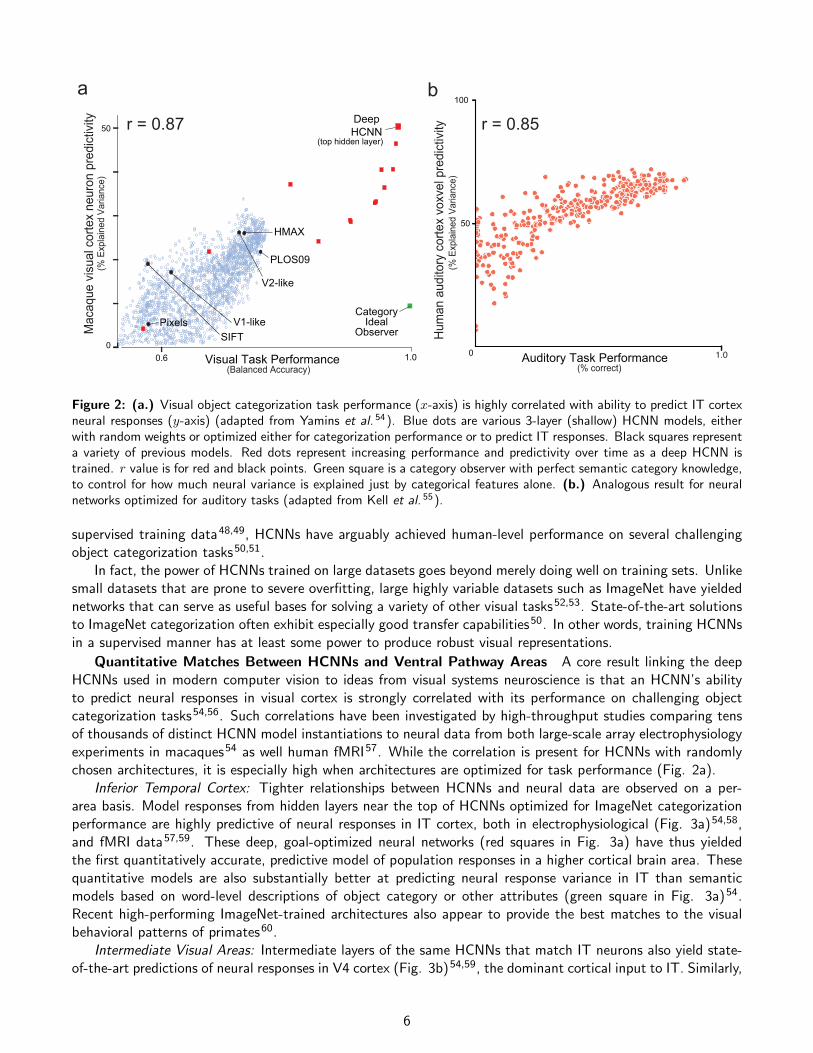
Figure 2: (a.) Visual object categorization task performance (x-axis) is highly correlated with ability to predict IT cortexneural responses (y-axis) (adapted from Yamins et al. 54). Blue dots are various 3-layer (shallow) HCNN models, eitherwith random weights or optimized either for categorization performance or to predict IT responses. Black squares representa variety of previous models. Red dots represent increasing performance and predictivity over time as a deep HCNN istrained. r value is for red and black points. Green square is a category observer with perfect semantic category knowledge,to control for how much neural variance is explained just by categorical features alone. (b.) Analogous result for neuralnetworks optimized for auditory tasks (adapted from Kell et al. 55).
supervised training data48,49, HCNNs have arguably achieved human-level performance on several challengingobject categorization tasks50,51.
In fact, the power of HCNNs trained on large datasets goes beyond merely doing well on training sets. Unlikesmall datasets that are prone to severe overfitting, large highly variable datasets such as ImageNet have yieldednetworks that can serve as useful bases for solving a variety of other visual tasks52,53. State-of-the-art solutionsto ImageNet categorization often exhibit especially good transfer capabilities50. In other words, training HCNNsin a supervised manner has at least some power to produce robust visual representations.
Quantitative Matches Between HCNNs and Ventral Pathway Areas A core result linking the deepHCNNs used in modern computer vision to ideas from visual systems neuroscience is that an HCNN’s abilityto predict neural responses in visual cortex is strongly correlated with its performance on challenging objectcategorization tasks54,56. Such correlations have been investigated by high-throughput studies comparing tensof thousands of distinct HCNN model instantiations to neural data from both large-scale array electrophysiologyexperiments in macaques54 as well human fMRI57. While the correlation is present for HCNNs with randomlychosen architectures, it is especially high when architectures are optimized for task performance (Fig. 2a).
Inferior Temporal Cortex: Tighter relationships between HCNNs and neural data are observed on a per-area basis. Model responses from hidden layers near the top of HCNNs optimized for ImageNet categorizationperformance are highly predictive of neural responses in IT cortex, both in electrophysiological (Fig. 3a)54,58,and fMRI data57,59. These deep, goal-optimized neural networks (red squares in Fig. 3a) have thus yieldedthe first quantitatively accurate, predictive model of population responses in a higher cortical brain area. Thesequantitative models are also substantially better at predicting neural response variance in IT than semanticmodels based on word-level descriptions of object category or other attributes (green square in Fig. 3a)54.Recent high-performing ImageNet-trained architectures also appear to provide the best matches to the visualbehavioral patterns of primates60.
Intermediate Visual Areas: Intermediate layers of the same HCNNs that match IT neurons also yield state-of-the-art predictions of neural responses in V4 cortex (Fig. 3b)54,59, the dominant cortical input to IT. Similarly,
6

recent models with especially good performance have distinct layers clearly segregating late-intermediate visualarea PIT neurons from downstream central IT (CIT) and AIT neurons61. These results are important becausethey show that high-level ecologically-relevant constraints on network function — ie. the categorization taskimposed at the network’s output layer — are strong enough to inform upstream visual features in a non-trivialway. In other words, HCNN models suggest that the computations performed by the circuits in V4 are structuredso that downstream computations in AIT can support high-variation robust categorization tasks. Thus, eventhough there may be no simple word-model describing what the features in an intermediate cortical area suchas V4 are, HCNNs can provide a principled description of why the area’s neural responses might be as they are.
Early Visual Cortex: Results in early visual cortex are equally striking. The filters emergent in HCNNs’early layers from the learning process naturally resemble Gabor wavelets without having to build this structurein48. Extending the correspondence between HCNN layers and ventral stream layers down further, it has beenshown that lower HCNN layers match neural responses in early visual cortex areas such as V1 (Fig. 3c)57,59,62.In fact, recent high-resolution results show that early-intermediate layers of performance-optimized HCNNs aresubstantially better models of macaque V1 neural responses to natural images than previous state-of-the-artmodels that were hand-designed to replicate qualitative neuroscience observations63.
Taken together, these results indicate that combining two general biological constraints — the behavioralconstraint of object recognition performance, and the architectural constraint imposed by the HCNN modelclass — leads to improved models of multiple areas through the visual pathway hierarchy.
A Contrast to Curve Fitting A key feature of these results is that the parameters of the HCNN modelsare optimized to solve a visual performance goal that is ethologically plausible for the organism, rather thanbeing directly fit to neural data. Yet, the resulting neural network effectively models the biology as well orbetter than direct curve fits54,63. This is the idea of goal-driven modeling43. Goal-driven modeling is attractiveas a method for building quantitative cortical models for several reasons. Practically speaking, it does notrequire the collection of the unrealistically massive amounts of neurophysiological data that would be neededto fit deep networks to such data. Second, because model validity is assessed on a completely different metric(and different dataset) than the one used to choose model parameters, the results are comparatively freefrom overfitting and/or multiple-comparison problems. Finally, the approach posits an evolutionally plausiblefunctional reason for choices of model parameters throughout the hierarchy.
A Tripartite Optimization FrameworkWhile the results described in the previous section are in some ways specific to the primate ventral pathway,
they are based on a more general underlying logic that can apply to neural network modeling problems throughoutcomputational neuroscience. Specifically, three fundamental components underlie all functionally-optimizedneural network models:• An architecture class A containing potential neural network structures from which the real system is
drawn. A captures the structural constraints on the network drawn from knowledge about a brain system’sanatomical and functional connectivity.• A computational goal that the system seeks to accomplish, mathematically expressed as a loss target
functionL : A −→ R
to be minimized by parameter choices within the set A. For any potential network a ∈ A, the value L(a)represents the error that network incurs in attempting to solve the computational goal. L captures thefunctional constraints on the network drawn from hypotheses about the organism’s behavioral repertoire.• A learning rule by which optimization for L occurs within the architecture class A. This is a function
RL : A −→ A
such that, at least statistically, for any non-optimal network A ∈ A,
L(RL(A)) < L(A). (3)
7

0
50
Pix
els
V1-
Like
PLO
S09
HM
AX
V2-
Like
SIF
T
0
50
1 3 5 7Controlmodels
macaque IT macaque V4
Idealobservers
HCNNlayers
Controlmodels
Idealobservers
HCNNlayers
Pix
els
V1-
Like
PLO
S09
HM
AX
V2-
Like
SIF
T 13 5 7
Cat
egor
yA
ll va
riabl
es
human V1-V3Si
ngle
-site
neu
ral p
redi
ctiv
itya c
0
0.4
HCNN Layers1 2 3 4 5 6 7pixels
b(%
Exp
lain
ed V
aria
nce)
Rep
rese
ntat
iona
l Sim
ilarit
y(K
enda
ll’s ta
u)
Figure 3: (a.) Based on Yamins et al. 54 , comparison of ability of various computational models to predict neural responsesof populations of macaque IT neurons (right). The HCNN model (red bars) is a significant improvement in neural responseprediction compared to previous models (black bars) and task ideal observers (green bars). The top HCNN layer 7 bestpredicts IT responses. (b.) Similar to a., but for macaque V4 neurons. Note that intermediate layer 5 best predicts V4responses.(c.) Representational similarity between visual representations in HCNN model layers and human V1-V3, basedon fMRI data (adapted from Khaligh-Razavi & Kriegeskorte 57). Horizontal gray bar represents the inherent noise ceilingof the data. Note that earlier HCNN model layers most resemble early visual areas.
Biologically, the learning rule captures the way that the error signal from mismatches between the system’scurrent output and the correct outputs (as as defined by the computational goal) is used to identify betterparameter choices, over evolutionary and developmental timeframes.
This framework predicts that, statistically, the actual biologically-observed system is approximated by the optimalsolution within A to the goal posed by L, i.e.
A∗ = argminA∈A
L(A), (4)
to the extent that the optima is actually reachable from chosen initial conditions via the learning rule. Ofcourse, biological systems produced by evolution and development are not guaranteed to be optimal for theirevolutionary niche, so this prediction is really more an informed heuristic for hypothesis generation rather thana candidate natural law. In fact, any practically implementable learning rule will not perfectly meet the criterionin eq. 3, being subject to the same problem that evolution/development faces: failures to achieve optimumdue to incomplete optimization or capture by local minima. Insofar as the model of the learning rule and initialcondition distribution is itself biologically accurate, the same patterns of performance failures should be observedin both the model and the real behavioral data60.
Returning to the example of the primate ventral stream, the model architecture class A has been takento include feedforward HCNNs, broadly capturing aspects of the known neuroanatomical structure of ventralvisual pathway. The parameters describing this class of models include (1) discrete choices about (e.g.) thenumber of layers in the cascade, the specific nonlinear operations to employ at each layer, and the sizes of localreceptive fields (see Yamins & DiCarlo 43 for more details on these parameters), and (2) the continuous-valuedfilter templates embodied by the linear transforms Li at each layer. The loss target L has typically been chosenas categorization error on the 1000-way object recognition task in the ImageNet dataset47, capturing the factthat primates have especially strong invariant object recognition capacities.
The learning rule used for optimizing HCNNs to solve categorization problems is composed of two pieces,corresponding to the two types of model parameters: (1) an “outer loop” of metaparameter optimization usedfor selecting the discrete parameters, typically either just random choice40 or a simple evolutionary algorithm54,and (2) an “inner loop” of smooth optimization of the synaptic strength parameters Li, typically involvinggradient descent:
dLi
dt= −λ(t) · ∇Li [L]. (5)
8

This expression formalizes the idea that learning modifies the synaptic strengths Li of the visual system overtime — the derivative dLi/dt — by greedily seeking to minimize the value of the loss target, scaled in magnitudeby the learning rate λ(t).
There are many variants of gradient descent that have been explored in the machine learning literature, someof which scale better or achieve faster or better optimization64–66. Though Hebbian learning rules have beenproposed many times in neuroscience67,68 and have attractive theoretical properties69, explicit error-based rulessuch as gradient descent have proven substantially more computationally effective. There is much debate aboutthe biological realism of gradient descent70, and an ongoing area of research seeks to discover more biologicallyplausible versions of explicit error-driven learning rules71,72.
While a vast oversimplification, the relationship between optimizing discrete architecture parameters andsynaptic strength parameters is somewhat analogous to the relationship between evolutionary and developmentallearning. Changes to synaptic strengths are continuous and can occur without modifying the overall systemarchitecture, and thus could support experience-driven optimization during the lifetime of the organism. Changesin the discrete parameters, in contrast, restructure the computational primitives, the number of sensory areas(model layers) and the number of neurons in each area, and thus are more likely to be selected over evolutionarytime.
Mapping Models to Data A goal-optimized model generates computationally precise hypotheses for howdata collected from the real system will look. Testing these hypotheses involves assessing metrics of similaritybetween the model and the brain system, both for the output behaviors of the system, as well as for internalresponses of the system’s neural components. Several commonly-used metrics for assessing the mapping ofmodels to empirical data include (from coarsest to finest resolution):
• Behavioral consistency. Even before any neural data is collected, high-throughput systematic measurementsof psychophysical data can be used obtain a “fingerprint” of human behavioral responses across a wide varietytask conditions60. This fingerprint can then be compared to output behavior on these tasks as generatedby neural network models. For example, Rajalingham et al. 60 show that achieving consistency with high-resolution human error patterns in visual categorization tasks is a very strong test of correctness for modelsof the primate visual system.• Population-level neural comparison. The Representation Dissimilarity Matrix (RDM) is a convenient tool for
comparing two neural representations at a population level73. Each entry in the RDM corresponds to onestimulus pair, with high/low values indicating that the population as a whole treats the pair stimuli as verydifferent/similar. Taken over the whole stimulus set, the RDM characterizes the layout of the images in thehigh-dimensional neural population space. A measure of how similar the representations are between realneural populations and those produced by a neural network can be obtained by assessing the correlationsbetween the RDMs from each layer of a neural network models and the RDMs from real neural populations.This technique, which is called Representational Similarity Analysis (RSA), has been effectively used forcomparing visual representations in human fMRI data to HCNN models57.• Single-neuron regression. Linear regression is a convenient method for mapping units from neural network
models to individual neural recording sites54. For each neural site, this technique seeks to identify a linearweighting of neural network model output units (typically from one network layer) that is most predictiveof that neural site’s actual output on a fixed set of sample images. The “synthetic neuron” then producesresponse predictions on novel stimuli not used in the regression training, which are then compared to theactual neural site’s output. Accuracy in regression prediction has shown to be a useful tool for achievingfiner-grained model-brain mappings when higher resolution (e.g. electrophysiological) data is available54,61.
See Yamins & DiCarlo 43 for a more detailed description and evaluation of these and other mapping procedures.
Properly Assessing Model Complexity When comparing any two models of data, it is important toensure that model complexity is taken into account: a complex model with many parameters may not be animprovement over a simple model with fewer parameters, even if the former has a somewhat better fit to the data.However, even though goal-optimized deep neural networks have many parameters before task optimization,those parameters are determined by the optimization process in attempting to solve the computational goalitself. Thus, when the optimized networks are subsequently mapped to brain data, these parameters are no longer
9

available for free modification to fit the neurons. Hence, although it may at first be somewhat counterintuitive,these pre-determined parameters cannot be counted when assessing model complexity, e.g. when computingscores such as the Akaike or Bayesian Information Criteria74. Instead, once the optimized network has beenproduced, the only free parameters used when comparing to neural data are just those required by the mappingprocedure itself. For example, when using Representational Similarity Analysis, no free parameters are neededat all, since building the RDM matrix requires is a parameter-free procedure. Thus, if a larger goal-optimizedneural network achieves between match between its RDMs and those in neural populations, it has done so fairly— that is, not by using those parameters to better (over)fit the neural data, but instead because the biggernetwork has (presumably) achieved better performance on the computational goal, and the computational goalis itself highly relevant to the real biological constraints on the neural mechanism. Similarly, when performingsingle-neuron regression, the number of free parameters is equal to the number of model neurons used as linearregressor dimensions. In this case, it is necessary (but easy) to ensure fair comparisons between models withdifferent numbers of features by simply subsampling a fixed number of model units as regressors (as done in e.g.Yamins et al. 54) or using some unsupervised dimension reduction procedure (such as PCA) prior to regression.
Relationship to Previous Work in Visual Modeling Other approaches to modeling the visual systemcan be placed in context of the optimization framework. Efficient coding hypotheses seek to generate efficient,low-dimensional representations of natural input statistics. This corresponds to a choice of architecture classA containing “hourglass-shaped” networks75 composed of a compressive intermediate encoding followed by adecoding that produces image-like output. The loss target is then (roughly) of the form:
L(x) = ||x−D(E(x))||+ Regularization(E(x))
where E(x) is the network encoding of image x, and D is the corresponding decoding. The first term of L isthe reconstruction error, measuring the ability of the decoded representation to reproduce the original input,while the second term prevents overfitting by imposing a “simpleness prior” on the encoder. Efficient codingis an attractive idea because it combines functional requirements and biophysical constrains (e.g. metabolicefficiency). Early versions of this idea such as sparse autoencoders76 have shown promise in training shallow(one-layer) convolutional networks that naturally discover the Gabor-like filter patterns seen in V1 cortex. Morerecent methods such as variational autoencoders, generative adversarial networks (GANs) and BiGANs77–79,essentially correspond to improvements in the choice of regularization functions, and have shown promise intraining deeper networks. While such ideas have been effective in limited visual domains, improving theirapplicability to unrestricted visual image space is an open question, and an important area for innovation80.
Another line of work has attempted to fit neural networks directly to data from V181, V282, and V483
cortex. These results are consistent with the optimization framework insofar as they involve finding parametersthat optimize a loss function — in this case, the mismatch between network output and the measured neuraldata. Such investigations can be very informative, as they contribute to the discovery of which classes of neuralarchitectures best capture the data. However, unlike the goal-driven modeling approach, or the efficient codingideas, these direct curve-fits do not generate a normative explanation underlying why the neural responses areas they are.
An interesting approach combines neural fits and normative explanations. In McIntosh et al. 84 , comparativelyshallow HCNNs were fit to responses in retinal ganglion cells (RGCs). A key finding in this work was thatcharacteristic properties of bipolar cells, which are upstream of the RGCs, naturally emerge in the networks’first layers, just by forcing the network’s last layer to correctly emulate RGC response patterns. While this workdoes not explain why the RGCs are as they are, it does suggest a kind of conditional normative explanationfor why the bipolar cell patterns are as they are, given the RGC as output. Understanding whether this holdsfor other parts of the retinal circuit (e.g the intermediate cells in the amacrine layer), and whether the RGCpatterns themselves arise from a higher-level downstream computational goal, are exciting open questions.
Beyond the Visual System The goal-driven optimization approach has also had success building quan-titatively accurate models of the human auditory system55,85. Using HCNNs as the architecture class, butsubstituting a computational goal defined by speech and music genre recognition, this work finds a strongcorrelation between auditory task performance and auditory cortex neural response predictivity (Fig. 2b). A
10

representational hierarchy is also found in auditory cortex, suggesting interesting similarities to the visual sys-tem, in that the robustness to variability (e.g. position, size, and pose tolerance) that makes convolutionalnetworks useful for visual object recognition may have rough equivalents in the auditory domain that makeconvolution useful for parsing auditory “objects”. However, the work of Kell et al. 55 goes beyond models ofa single processing stream, exhibiting multi-stream networks that solve several auditory tasks simultaneouslywith an initial common architecture that subsequently splits into multiple task-specific pathways. The differentpathways of the network differentially explain neural variance in different parts of auditory cortex, illustratinghow task-optimized neural networks can help further understanding of large-scale functional organization in thebrain. Recent work has begun to tackle somatosensory systems along similar lines86.
A functionally-driven optimization approach has also been effective at driving progress in modeling the motorsystem87,88. This work shows how imposing the computational goal of creating behaviorally-useful motor outputconstrains internal neural network components to match otherwise non-obvious features of neurons in motorcortex, and provides a modern computational basis for earlier work on movement efficiency89. Unlike work onsensory systems, the goals in motor networks are not representational, but instead focus on the generation ofdynamic patterns of motor prepration and movement90. For this reason, the models involved in these effortsare typically recurrent neural networks (RNNs) rather than feedforward HCNNs. These results show that thegoal-driven optimization idea has power across a wide range of network architectures and behavioral goal types.
Analyzing Constraints Rather Than Optima A classic approach to analyzing a population of (in mostcases, sensory) neurons is to classify the shape of their tuning curves in response to systematically changing inputstimuli along certain characteristic axes that are key drivers of the populations’ variability. This approach hasbeen successful in a variety of brain areas, most notably in early visual cortex27, where tuning curves illustratingthe orientation and frequency selectivity of V1 neurons laid the groundwork for Gabor-wavelet based models.
Relative to the optimization framework described above, the analysis of tuning curves is essentially an attemptto characterize optimal networks A∗ in non-optimization-based terms. When a small number of mathematically-simple stimulus-domain axes can be found in which the tuning curves of A∗ have a mathematically-simple shape,A∗ can largely be constructed by a simple closed-form procedure without any reference to learning through it-erative optimization. This is to some extent feasible for V1 neurons, and perhaps in early cortical areas in otherdomains such as primary auditory cortex91. It is possible that this type of simplification is most helpful for under-standing neural responses that arise largely from highly constrained stereotyped genetic developmental programsrather than those that depend heavily on experience-driven learning92, or where biophysical constraints — suchas metabolic cost or noise reduction — might also impose “simplicity priors” on the neural architecture76,87.
In general, however, it is not guaranteed that closed-form expressions describing the response propertiesof task-optimized models can be found. Evolution and development are under no general constraint to maketheir products conform to simple mathematical simple shapes, especially for intermediate and higher corticalareas at a remove from the sensory or motor periphery. However, even if such analytical simplifications donot exist, the optimization framework nonetheless provides a method for generating meta-understanding viacharacterizing the constraints on the system, rather than analyzing the specific outcome network itself. Byvarying the architectural class, the computational goal, or the learning rule, and identifying which choices leadto networks that best match the observed neural data, it is possible to learn much about the brain system ofinterest even if its tuning curves are inscrutable.
Understanding Multiple Optima What happens when multiple optimal network solutions exist? Formany architecture classes there may be infinitely many qualitatively very similar networks with the same orsubstantially similar outputs — e.g. those created by applying orthonormal rotations to linear transforms presentin the network. Sometimes, however, qualitatively very distinct networks might achieve similar performance levelson a task. For example, very deep Residual Network architectures51 and comparatively shallower (but much morelocally complex) architectures arising from Neural Architecture Search50 achieve roughly similar performanceon ImageNet categorization despite key structural differences.
The optimization framework does not require there be a unique best solution to the computational goalto make useful predictions. If several subclasses of high-performing solutions to a given task are identified,this is equivalent to formulating multiple very qualitatively distinct hypotheses for the neural circuits underlying
11
function in a given brain area. Recent work in modeling rodent whisker-trigeminal cortex, in which similar taskperformance on whisker-driven shape recognition can be achieved by several distinct neural architecture classes,illustrates this idea86. Comparison of the distinct model types to experimental results either from detailedbehavioral or neural experiments is then likely to point toward one of these hypotheses as explaining the databetter than others. Techniques similar to those used to create the models in the first place can be deployed togenerate optimal stimuli for separating the predictions of the multiple models as widely possible, which wouldin turn directly inform experimental design. In these cases, the optimization framework serves as an efficientgenerator of strong hypotheses.
In contrast, if most high-performing solutions to a computational goal fall into a comparatively narrowerband of variability, the set of model solutions may correspond to actual variability in the the real subjectpopulation. For some brain regions, especially those in intermediate or higher cortical areas, the particularcollection of neural circuits present in any one subject’s brain may vary considerably between conspecifics93.The optimization framework naturally supports at least two potential sources of such variation, including:• Variation of initial conditions, described as a probability distribution over starting point models A0 to
which the learning rule is applied. For example, different random draws of initial values for linear filters Li
will lead to distinct final optimized HCNNs. While many high-level representational properties are sharedbetween these networks, meaningful differences can exist94, and may explain aspects of the variationbetween real visual systems.• Variation of computational goal, described as a distribution over stimuli in the dataset defining the goal
task. This idea captures the concept that different individuals will experience somewhat different stimulusdiets during development and learning.
Understanding the computational sources of intra-specific variation is itself an important modeling question forfuture work95.
A Contravariance Principle Though it may at first seem counterintuitive, the harder the computationalgoal, the easier the model-to-brain matching problem is likely to be. This because the set of architecturalsolutions to an easy goal is large, while the set of solutions to a challenging goal is comparatively smaller. Inmathematical terms, the size of the set of optima is contravariant in the difficulty of the optimization problem.
A simple thought experiment makes this clear: imagine if, instead of trying to solve 1000-way objectclassification in the real-world ImageNet dataset, one simply asked a network to solve binary discriminationbetween two simple geometric shapes shown on uniform gray backgrounds. The set of networks that can solvethe latter task is much less narrowly constrained than that which solve the former. And given that primatesactually do exhibit robust object classification, the more strongly constrained networks that pass the same harderperformance tests are more likely to be homologous to the real primate visual system. A detailed example of howoptimizing a network to achieve high performance on a low-variation training set can lead to poor performancegeneralization and neurally inconsistent features is illustrated in *Hong et al. 35 .
The contravariance principle makes a strong prescription for using the optimization framework to designeffective computationally-driven experiments. Unlike the typical practice in experimental neuroscience, butechoing recent theoretical discussions of task dimensionality Gao et al. 96 , it does not make sense from theoptimization perspective to choose the most reduced version of a given task domain and then seek to thoroughlyunderstand the mechanisms that solve the reduced task before attempting to address more realistic versions ofthe task. In fact, this sort of highly reductive approach is likely to lead to confusing results, precisely becausethe reduced task may admit many spurious solutions. Instead, it is more effective to impose the challengingreal-world task from the beginning, both in designing training sets for optimizing the neural network models, andin designing experimental stimulus sets for making model-data comparisons. Even if the absolute performancenumbers of networks on the harder computational goal are lower, the resulting networks are likely to be bettermodels of the real neural system.
There is a natural balance between network size and capacity. In general, the optimization-based approachis likely to be most efficient when the network sizes are just large enough to solve the computational task. Thus,another way to constrain networks while still using a comparatively simple computational goal is to reduce thenetwork size. This idea is consistent with results from experiments measuring neural dynamics in the fruit fly,
12

where a small but apparently near-optimal circuit has been shown to be responsible for the fly’s simple but robustnavigational control behaviors97. It remains unknown whether the specific architectural principles discoveredin such simplified settings will prove useful for understanding the larger networks needed for achieving moresophisticated computational goals in higher organisms.
Major Future DirectionsThe optimization framework suggests a wide variety of important future directions to be explored.
Better Sensory Models. Within the domain of the visual system, there are many substantial differencesremaining between state-of-the-art models and the real neural system. For neurons throughout the macaqueventral visual stream, the best neural network models are able to explain only approximately 65 percent of thereliable time-averaged neural responses to static natural stimuli. This neural result is echoed by the fact thatwhile the models are behaviorally consistent with primate and human visual error patterns at the category orobject level32, they fail to entirely account for error patterns at a the finest image-by-image grain60, especiallyin the context of adversarially-created stimuli98. Closing the explanatory gap will require a next generation ofimproved models.
Another major open direction involves understanding recurrence and feedback in visual (and other sensory)processing, and the corresponding modeling of neurons’ temporal dynamics. While some recent progress has beenmade on functionally-driven neural models of temporal dynamics that integrate RNN motifs into HCNNs61,99, itit is unlikely that a full understanding of the functional role of feedback has been achieved. While most modelingefforts have so far focused on the ventral visual pathway, understanding the functional demands that lead tothe emergence of multiple visual pathways, or combining constraints at multiple levels (e.g. behavioral andbiophysical), is another key direction for future work. Likewise, little attention has been paid to understandingthe physical layout of brain areas. While some of the most robust results in human cognitive neuroscience involvethe identification of subregions of visual cortex that selectively respond to certain classes stimuli, e.g. the well-known face, body and place areas100–102, the computational-level constraints leading to these topographicalfeatures are poorly understood.
Learning. Though the optimization framework has shown exciting progress at the intersection of machinelearning and computational neuroscience, there is a fundamental problem confronting the approach. Typicalneural network training uses heavily supervised methods involving huge numbers of high-level semantic labels,e.g. category labels for thousands examples in each of thousands of categories47,103. Viewed as technicaltools for tuning algorithm parameters, such procedures can be acceptable, although they limit the purview ofthe method to situations with large existing labelled datasets. As real models of learning in the brain, theyare highly unrealistic, because, among other reasons, human infants and non-human primates simply do notreceive millions of category labels during development. There has been a substantial amount of research onunsupervised, semi-supervised, and self-supervised visual learning methods76–78,104–106. Despite these advances,the gap between supervised and unsupervised approaches still remains significant. The discovery of proceduresthat are computationally powerful but use substantially less labelled data is a key challenge for understandinglearning real biological learning.
Modeling Integrated Agents Rather Than Isolated Systems. Cognition is not just about the passiveparsing of sensory streams or disembodied generation of motor commands. Humans are agents, interactingwith and modifying their environment via a tight visuomotor loop. Effective courses of action based both onsensory input and the agent’s goals afford the agent the opportunity to restructure its surroundings to betterpursue those goals. By the same token, however, constructing and evaluating a complex action policy imposesa substantial additional computational challenge for the agent that goes considerably beyond “mere” sensoryprocessing. Applying the optimization framework to modeling full agents is an exciting possibility, and somerecent speculative work in deep reinforcement learning has made progress in direction107,108. However, fullyfleshing out neural network models of memory, decision making, higher cognition that have the resolution andcompleteness to be quantitatively compared to experimental data will require substantial improvements at thealgorithmic level.
The problem of learning becomes especially acute in the context of interactive systems. Human infants
13

employ an active learning process that builds representations underlying sensory judgments and motor plan-ning109–111. Children exhibit a wide range of interesting, apparently spontaneous, visuo-motor behaviors —including navigating their environment, seeking out and attending to novel objects, and engaging physicallywith these objects in novel and surprising ways110–116. Modeling these key behaviors, and the brain systemsthat underly them, is a formidable challenge for computational cognitive neuroscience117.
14

References1. DiCarlo, J. J., Zoccolan, D. & Rust, N. C. How does the brain solve visual object recognition? Neuron
73, 415–34 (2012).
2. James, W. The principles of psychology (Vol. 1). New York: Holt 474 (1890).
3. DiCarlo, J. J. & Cox, D. D. Untangling invariant object recognition. TICS (2007).
4. Malach, R., Levy, I. & Hasson, U. The topography of high-order human object areas. Trends in cognitivesciences 6, 176–184 (2002).
5. Felleman, D. & Van Essen, D. Distributed hierarchical processing in the primate cerebral cortex. CerebralCortex 1, 1–47 (1991).
6. Rust, N. C. & DiCarlo, J. J. Selectivity and tolerance (“invariance”) both increase as visual informationpropagates from cortical area V4 to IT. J Neurosci 30, 12978–95 (2010).
7. Connor, C. E., Brincat, S. L. & Pasupathy, A. Transformation of shape information in the ventral pathway.Curr Opin Neurobiol 17, 140–7 (2007).
8. Carandini, M., Demb, J. B., Mante, V., Tolhurst, D. J., Dan, Y., Olshausen, B. A., Gallant, J. L. & Rust,N. C. Do we know what the early visual system does? J Neurosci 25, 10577–97 (2005).
9. Movshon, J. A., Thompson, I. D. & Tolhurst, D. J. Spatial summation in the receptive fields of simplecells in the cat’s striate cortex. The Journal of physiology 283, 53–77 (1978).
10. Majaj, N. J., Hong, H., Solomon, E. A. & DiCarlo, J. J. Simple Learned Weighted Sums of InferiorTemporal Neuronal Firing Rates Accurately Predict Human Core Object Recognition Performance. TheJournal of Neuroscience 35, 13402–13418 (2015).
11. Yamane, Y., Carlson, E. T., Bowman, K. C., Wang, Z. & Connor, C. E. A neural code for three-dimensionalobject shape in macaque inferotemporal cortex. Nat Neurosci 11, 1352–1360 (2008).
12. Hung, C. P., Kreiman, G., Poggio, T. & Dicarlo, J. J. Fast readout of object identity from macaqueinferior temporal cortex. Science 310, 863–866 (2005).
13. Freeman, J. & Simoncelli, E. Metamers of the ventral stream. Nature Neuroscience 14, 1195–1201 (2011).
14. DiCarlo, J. J. & Cox, D. D. Untangling invariant object recognition. Trends Cogn Sci 11, 333–41 (2007).
15. Schmolesky, M. T., Wang, Y., Hanes, D. P., Thompson, K. G., Leutgeb, S., Schall, J. D. & Leventhal,A. G. Signal timing across the macaque visual system. J Neurophysiol 79, 3272–8 (1998).
16. Lennie, P. & Movshon, J. A. Coding of color and form in the geniculostriate visual pathway (invitedreview). J Opt Soc Am A Opt Image Sci Vis 22, 2013–33 (2005).
17. Schiller, P. Effect of lesion in visual cortical area V4 on the recognition of transformed objects. Nature376, 342–344 (1995).
18. Gallant, J., Connor, C., Rakshit, S., Lewis, J. & Van Essen, D. Neural responses to polar, hyperbolic, andCartesian gratings in area V4 of the macaque monkey. Journal of Neurophysiology 76, 2718–2739 (1996).
19. Brincat, S. L. & Connor, C. E. Underlying principles of visual shape selectivity in posterior inferotemporalcortex. Nat Neurosci 7, 880–6 (2004).
20. Yau, J. M., Pasupathy, A., Brincat, S. L. & Connor, C. E. Curvature processing dynamics in macaquearea V4. Cerebral Cortex 23, 198–209 (2012).

21. Sharpee, T. O., Kouh, M. & Reyholds, J. H. Trade-off between curvature tuning and position invariancein visual area V4. PNAS 110, 11618–11623 (2012).
22. Pickles, J. O. An Introduction to the Physiology of Hearing (2008).
23. Romanski, L. M. & LeDoux, J. E. Information cascade from primary auditory cortex to the amygdala:corticocortical and corticoamygdaloid projections of temporal cortex in the rat. Cerebral Cortex 3, 515–532(1993).
24. Hegner, Y. L., Lindner, A. & Braun, C. A somatosensory-to-motor cascade of cortical areas engaged inperceptual decision making during tactile pattern discrimination. Human brain mapping 38, 1172–1181(2017).
25. Petersen, C. C. The Functional Organization of the Barrel Cortex. Neuron 56, 339–355 (2007).
26. Wang, L., Mruczek, R. E., Arcaro, M. J. & Kastner, S. Probabilistic maps of visual topography in humancortex. Cerebral cortex 25, 3911–3931 (2014).
27. Hubel, D. H. & Wiesel, T. N. Receptive fields of single neurones in the cat’s striate cortex. The Journalof physiology 148, 574–591 (1959).
28. Ringach, D. L., Shapley, R. M. & Hawken, M. J. Orientation selectivity in macaque V1: diversity andlaminar dependence. Journal of Neuroscience 22, 5639–5651 (2002).
29. Willmore, B., Prenger, R. J., Wu, M. C.-K. & Gallant, J. L. The berkeley wavelet transform: a biologicallyinspired orthogonal wavelet transform. Neural computation 20, 1537–1564 (2008).
30. Poole, B., Lahiri, S., Raghu, M., Sohl-Dickstein, J. & Ganguli, S. Exponential expressivity in deep neuralnetworks through transient chaos. In Advances in neural information processing systems, 3360–3368(2016).
31. Bengio, Y. Deep learning of representations for unsupervised and transfer learning. In Proceedings ofICML Workshop on Unsupervised and Transfer Learning, 17–36 (2012).
32. Rajalingham, R., Schmidt, K. & DiCarlo, J. J. Comparison of object recognition behavior in human andmonkey. J. Neurosci. 35, 12127–36 (2015).
33. Freedman, D. J., Riesenhuber, M., Poggio, T. & Miller, E. K. Categorical representation of visual stimuliin the primate prefrontal cortex. Science 291, 312–316 (2001).
34. Pagan, M., Urban, L. S., Wohl, M. P. & Rust, N. C. Signals in inferotemporal and perirhinal cortex suggestan untangling of visual target information. Nature neuroscience 16, 1132–1139 (2013).
35. *Hong, H., *Yamins, D. L., Majaj, N. J. & DiCarlo, J. J. Explicit information for category-orthogonalobject properties increases along the ventral stream. Nature neuroscience 19, 613–622 (2016).
36. Nishio, A., Shimokawa, T., Goda, N. & Komatsu, H. Perceptual Gloss Parameters Are Encoded byPopulation Responses in the Monkey Inferior Temporal Cortex. The Journal of Neuroscience 34, 11143–11151 (2014).
37. Cover, T. M. & Thomas, J. A. Elements of information theory (John Wiley & Sons, 2012).
38. Pinto, N., Cox, D. D. & Dicarlo, J. J. Why is real-world visual object recognition hard? PLoS Computa-tional Biology (2008).
39. Tanaka, K. Columns for complex visual object features in the inferotemporal cortex: clustering of cellswith similar but slightly different stimulus selectivities. Cerebral Cortex 13, 90–99 (2003).

40. Pinto, N., Doukhan, D., DiCarlo, J. J. & Cox, D. D. A High-Throughput Screening Approach to DiscoveringGood Forms of Biologically Inspired Visual Representation. PLoS Comput Biol (2009).
41. Fukushima, K. Neocognitron: A self-organizing neural network model for a mechanism of pattern recog-nition unaffected by shift in position. Biological cybernetics 36, 193–202 (1980).
42. LeCun, Y. & Bengio, Y. Convolutional networks for images, speech, and time series. The handbook ofbrain theory and neural networks 255–258 (1995).
43. Yamins, D. L. & DiCarlo, J. J. Using goal-driven deep learning models to understand sensory cortex.Nature neuroscience 19, 356–365 (2016).
44. Serre, T., Oliva, A. & Poggio, T. A feedforward architecture accounts for rapid categorization. Proc NatlAcad Sci U S A 104, 6424–9 (2007). 0027-8424 (Print) Journal Article.
45. Carandini, M. & Heeger, D. J. Normalization as a canonical neural computation. Nature Reviews Neuro-science 13, 51–62 (2012).
46. Pinto, N., Doukhan, D., Dicarlo, J. J. & Cox, D. D. A high-throughput screening approach to discoveringgood forms of biologically inspired visual representation. PLoS Computational Biology 5 (2009).
47. Deng, J., Dong, W., Socher, R., Li, L.-J., Li, K. & Fei-Fei, L. ImageNet: A Large-Scale Hierarchical ImageDatabase. In CVPR09, 248–255 (2009).
48. Krizhevsky, A., Sutskever, I. & Hinton, G. E. Imagenet classification with deep convolutional neuralnetworks. In Advances in neural information processing systems, 1097–1105 (2012).
49. Bergstra, J., Yamins, D. & Cox, D. Making a science of model search: Hyperparameter optimization inhundreds of dimensions for vision architectures. In Proceedings of The 30th International Conference onMachine Learning, 115–123 (2013).
50. Zoph, B., Vasudevan, V., Shlens, J. & Le, Q. V. Learning transferable architectures for scalable imagerecognition. In Proceedings of the IEEE conference on computer vision and pattern recognition, 8697–8710(2018).
51. He, K., Zhang, X., Ren, S. & Sun, J. Deep residual learning for image recognition. In Proceedings of theIEEE conference on computer vision and pattern recognition, 770–778 (2016).
52. Simonyan, K. & Zisserman, A. Very deep convolutional networks for large-scale image recognition. arXivpreprint arXiv:1409.1556 (2014).
53. Girshick, R. Fast r-cnn. In Proceedings of the IEEE international conference on computer vision, 1440–1448(2015).
54. Yamins, D. L., Hong, H., Cadieu, C. F., Solomon, E. A., Seibert, D. & DiCarlo, J. J. Performance-optimized hierarchical models predict neural responses in higher visual cortex. Proceedings of the NationalAcademy of Sciences 111, 8619–8624 (2014).
55. Kell, A. J., Yamins, D. L., Shook, E. N., Norman-Haignere, S. V. & McDermott, J. H. A Task-OptimizedNeural Network Replicates Human Auditory Behavior, Predicts Brain Responses, and Reveals a CorticalProcessing Hierarchy. Neuron 98, 630–644 (2018).
56. Yamins, D. L., Hong, H., Cadieu, C. & DiCarlo, J. J. Hierarchical modular optimization of convolutionalnetworks achieves representations similar to macaque IT and human ventral stream. In Advances in neuralinformation processing systems, 3093–3101 (2013).

57. Khaligh-Razavi, S.-M. & Kriegeskorte, N. Deep supervised, but not unsupervised, models may explain ITcortical representation. PLoS computational biology 10, e1003915 (2014).
58. Cadieu, C. F., Hong, H., Yamins, D. L., Pinto, N., Ardila, D., Solomon, E. A., Majaj, N. J. & DiCarlo,J. J. Deep neural networks rival the representation of primate IT cortex for core visual object recognition.PLoS computational biology 10, e1003963 (2014).
59. Guclu, U. & van Gerven, M. A. Deep neural networks reveal a gradient in the complexity of neuralrepresentations across the ventral stream. The Journal of Neuroscience 35, 10005–10014 (2015).
60. Rajalingham, R., Issa, E. B., Bashivan, P., Kar, K., Schmidt, K. & DiCarlo, J. J. Large-scale, high-resolutioncomparison of the core visual object recognition behavior of humans, monkeys, and state-of-the-art deepartificial neural networks. Journal of Neuroscience 38, 7255–7269 (2018).
61. Nayebi, A., Bear, D., Kubilius, J., Kar, K., Ganguli, S., Sussillo, D., DiCarlo, J. J. & Yamins, D. L. Task-Driven convolutional recurrent models of the visual system. In Advances in Neural Information ProcessingSystems, 5290–5301 (2018).
62. Seibert, D., Yamins, D. L., Ardila, D., Hong, H., DiCarlo, J. J. & Gardner, J. L. A performance-optimized model of neural responses across the ventral visual stream. bioRxiv (2016). URL http:
//biorxiv.org/content/early/2016/01/12/036475.
63. Cadena, S. A., Denfield, G. H., Walker, E. Y., Gatys, L. A., Tolias, A. S., Bethge, M. & Ecker, A. S. Deepconvolutional models improve predictions of macaque V1 responses to natural images. PLoS computationalbiology 15, e1006897 (2019).
64. Bottou, L. Large-scale machine learning with stochastic gradient descent. In Proceedings of COMP-STAT’2010, 177–186 (Springer, 2010).
65. Zeiler, M. D. ADADELTA: an adaptive learning rate method. arXiv preprint arXiv:1212.5701 (2012).
66. Kingma, D. P. & Ba, J. Adam: A Method for Stochastic Optimization (2014).
67. Song, S., Miller, K. D. & Abbott, L. F. Competitive Hebbian learning through spike-timing-dependentsynaptic plasticity. Nature neuroscience 3, 919 (2000).
68. Montague, P. R., Dayan, P. & Sejnowski, T. J. A framework for mesencephalic dopamine systems basedon predictive Hebbian learning. Journal of neuroscience 16, 1936–1947 (1996).
69. Gerstner, W. & Kistler, W. M. Mathematical formulations of Hebbian learning. Biological cybernetics 87,404–415 (2002).
70. Stork, D. G. Is backpropagation biologically plausible. In International Joint Conference on Neural Net-works, vol. 2, 241–246 (IEEE Washington, DC, 1989).
71. Bengio, Y., Lee, D.-H., Bornschein, J., Mesnard, T. & Lin, Z. Towards biologically plausible deep learning.arXiv preprint arXiv:1502.04156 (2015).
72. Lillicrap, T. P., Cownden, D., Tweed, D. B. & Akerman, C. J. Random feedback weights support learningin deep neural networks. arXiv preprint arXiv:1411.0247 (2014).
73. Kriegeskorte, N., Mur, M., Ruff, D. A., Kiani, R., Bodurka, J., Esteky, H., Tanaka, K. & Bandettini, P. A.Matching categorical object representations in inferior temporal cortex of man and monkey. Neuron 60,1126–41 (2008).
74. Schwarz, G. et al. Estimating the dimension of a model. The annals of statistics 6, 461–464 (1978).

75. Hinton, G. E. & Salakhutdinov, R. R. Reducing the dimensionality of data with neural networks. science313, 504–507 (2006).
76. Olshausen, B. A. & Field, D. J. Emergence of simple-cell receptive field properties by learning a sparsecode for natural images. Nature 381, 607–609 (1996).
77. Kingma, D. P. & Welling, M. Auto-Encoding Variational Bayes (2013).
78. Goodfellow, I., Pouget-Abadie, J., Mirza, M., Xu, B., Warde-Farley, D., Ozair, S., Courville, A. & Bengio,Y. Generative adversarial nets. In Advances in neural information processing systems, 2672–2680 (2014).
79. Donahue, J., Krahenbuhl, P. & Darrell, T. Adversarial feature learning. arXiv preprint arXiv:1605.09782(2016).
80. Karras, T., Aila, T., Laine, S. & Lehtinen, J. Progressive growing of gans for improved quality, stability,and variation. arXiv preprint arXiv:1710.10196 (2017).
81. Klindt, D., Ecker, A. S., Euler, T. & Bethge, M. Neural system identification for large populationsseparating “what” and “where”. In Advances in Neural Information Processing Systems, 3506–3516(2017).
82. Vintch, B., Zaharia, A., Movshon, J. & Simoncelli, E. P. Efficient and direct estimation of a neural subunitmodel for sensory coding. In Advances in neural information processing systems, 3104–3112 (2012).
83. Cadieu, C., Kouh, M., Pasupathy, A., Connor, C. E., Riesenhuber, M. & Poggio, T. A model of V4 shapeselectivity and invariance. J Neurophysiol 98, 1733–50 (2007).
84. McIntosh, L., Maheswaranathan, N., Nayebi, A., Ganguli, S. & Baccus, S. Deep learning models ofthe retinal response to natural scenes. In Advances in neural information processing systems, 1369–1377(2016).
85. Guclu, U., Thielen, J., Hanke, M. & Van Gerven, M. Brains on beats. In Advances in Neural InformationProcessing Systems, 2101–2109 (2016).
86. Zhuang, C., Kubilius, J., Hartmann, M. J. & Yamins, D. L. Toward Goal-Driven Neural Network Modelsfor the Rodent Whisker-Trigeminal System. In Advances in Neural Information Processing Systems, 2555–2565 (2017).
87. Sussillo, D., Churchland, M. M., Kaufman, M. T. & Shenoy, K. V. A neural network that finds a naturalisticsolution for the production of muscle activity. Nature neuroscience 18, 1025–1033 (2015).
88. Lillicrap, T. P. & Scott, S. H. Preference distributions of primary motor cortex neurons reflect controlsolutions optimized for limb biomechanics. Neuron 77, 168–179 (2013).
89. Flash, T. & Hogan, N. The coordination of arm movements: an experimentally confirmed mathematicalmodel. Journal of neuroscience 5, 1688–1703 (1985).
90. Churchland, M. M., Cunningham, J. P., Kaufman, M. T., Foster, J. D., Nuyujukian, P., Ryu, S. I. &Shenoy, K. V. Neural population dynamics during reaching. Nature 487, 51 (2012).
91. Chi, T., Ru, P. & Shamma, S. A. Multiresolution spectrotemporal analysis of complex sounds. The Journalof the Acoustical Society of America 118, 887–906 (2005).
92. Espinosa, J. S. & Stryker, M. P. Development and plasticity of the primary visual cortex. Neuron 75,230–249 (2012).

93. Baldassarre, A., Lewis, C. M., Committeri, G., Snyder, A. Z., Romani, G. L. & Corbetta, M. Individualvariability in functional connectivity predicts performance of a perceptual task. Proceedings of the NationalAcademy of Sciences 109, 3516–3521 (2012).
94. Li, Y., Yosinski, J., Clune, J., Lipson, H. & Hopcroft, J. Convergent Learning: Do different neuralnetworks learn the same representations? In NIPS Workshop on Feature Extraction: Modern Questionsand Challenges, 196–212 (2015).
95. Van Horn, J. D., Grafton, S. T. & Miller, M. B. Individual variability in brain activity: a nuisance or anopportunity? Brain imaging and behavior 2, 327–334 (2008).
96. Gao, P., Trautmann, E., Byron, M. Y., Santhanam, G., Ryu, S., Shenoy, K. & Ganguli, S. A theory ofmultineuronal dimensionality, dynamics and measurement. bioRxiv 214262 (2017).
97. Turner-Evans, D., Wegener, S., Rouault, H., Franconville, R., Wolff, T., Seelig, J. D., Druckmann, S. &Jayaraman, V. Angular velocity integration in a fly heading circuit. Elife 6, e23496 (2017).
98. Kurakin, A., Goodfellow, I. & Bengio, S. Adversarial examples in the physical world. arXiv preprintarXiv:1607.02533 (2016).
99. Spoerer, C. J., McClure, P. & Kriegeskorte, N. Recurrent convolutional neural networks: a better modelof biological object recognition. Frontiers in psychology 8, 1551 (2017).
100. Kanwisher, N., McDermott, J. & Chun, M. M. The fusiform face area: a module in human extrastriatecortex specialized for face perception. J Neurosci 17, 4302–11 (1997).
101. Downing, P., Jiang, Y., Shuman, M. & Kanwisher, N. A Cortical Area Selective for Visual Processing ofthe Human Body. Science 293, 2470–2473 (2001).
102. Epstein, R. & Kanwisher, N. A cortical representation of the local visual environment. Nature 392,598–601 (1998).
103. Mahajan, D., Girshick, R., Ramanathan, V., He, K., Paluri, M., Li, Y., Bharambe, A. & van der Maaten,L. Exploring the limits of weakly supervised pretraining. In Proceedings of the European Conference onComputer Vision (ECCV), 181–196 (2018).
104. Tarvainen, A. & Valpola, H. Mean teachers are better role models: Weight-averaged consistency targetsimprove semi-supervised deep learning results. In Advances in neural information processing systems,1195–1204 (2017).
105. Settles, B. Active Learning, vol. 18 (Morgan & Claypool Publishers, 2011).
106. Sener, O. & Savarese, S. A Geometric Approach to Active Learning for Convolutional Neural Networks.CoRR abs/1708.00489 (2017).
107. Wayne, G., Hung, C.-C., Amos, D., Mirza, M., Ahuja, A., Grabska-Barwinska, A., Rae, J., Mirowski, P.,Leibo, J. Z., Santoro, A. et al. Unsupervised Predictive Memory in a Goal-Directed Agent. arXiv preprintarXiv:1803.10760 (2018).
108. Yang, G. R., Ganichev, I., Wang, X.-J., Shlens, J. & Sussillo, D. A dataset and architecture for visualreasoning with a working memory. arXiv preprint arXiv:1803.06092 (2018).
109. Kidd, C., Piantadosi, S. T. & Aslin, R. N. The Goldilocks Effect: Human Infants Allocate Attention toVisual Sequences That Are Neither Too Simple Nor Too Complex. PLOS ONE 7, 1–8 (2012).
110. Goupil, L., Romand-Monnier, M. & Kouider, S. Infants ask for help when they know they don’t know.Proceedings of the National Academy of Sciences 113, 3492–3496 (2016).

111. Begus, K., Gliga, T. & Southgate, V. Infants Learn What They Want to Learn: Responding to InfantPointing Leads to Superior Learning. PLOS ONE 9, 1–4 (2014).
112. Fantz, R. L. Visual experience in infants: Decreased attention to familiar patterns relative to novel ones.Science 146, 668–670 (1964).
113. Twomey, K. E. & Westermann, G. Curiosity-based learning in infants: a neurocomputational approach.Developmental Science 21 (2018).
114. Hurley, K. B., Kovack-Lesh, K. A. & Oakes, L. M. The influence of pets on infants’ processing of cat anddog images. Infant Behav Dev 33, 619–628 (2010).
115. Hurley, K. B. & Oakes, L. M. Experience and distribution of attention: Pet exposure and infants’ scanningof animal images. J Cogn Dev 16, 11–30 (2015).
116. Gopnik, A., Meltzoff, A. & Kuhl, P. The Scientist In The Crib: Minds, Brains, And How Children Learn(HarperCollins, 2009).
117. Haber, N., Mrowca, D., Fei-Fei, L. & Yamins, D. L. Learning to Play with Intrinsically-Motivated Self-Aware Agents (2018).