an overset adaptive high-order approach for blade-resolved wind energy...
TRANSCRIPT
An Overset Adaptive High-Order Approach for Blade-Resolved Wind EnergyApplications
Andrew KirbyDoctoral Candidate
University of WyomingLaramie, WY, USA
Michael BrazellPostdoctoral ResearcherUniversity of Wyoming
Laramie, WY, USA
Jay SitaramanAerospace Engineer
Parallel Geometric Algorithms LLCSunnyvale, CA, USA
Dimitri MavriplisProfessor
University of WyomingLaramie, WY, USA
ABSTRACTAn overset dual-mesh, dual-solver for computational fluid dynamics (CFD) is presented for wind energy applications.The dual-mesh paradigm is implemented in a near-body/off-body mesh system utilizing an unstructured mesh for thenear-body and a Cartesian mesh for the off-body. The dual-solver paradigm uses variable-order, mixed-discretizationsolvers optimized for the respective near-body/off-body grids. Preliminary results of a computational study of the Na-tional Renewable Energy Laboratory (NREL) Phase VI wind turbine are presented. Results for uniform axial inflowvelocities (7, 10, and 15 m/s) compare computed and measured results, including total power and thrust, sectionalpressure coefficient, and a down-stream wake deficit profile for a uniform axial inflow velocity of 10 m/s. Qualitativeresults are presented for a dynamically mesh adaptive off-body solver in the dual-mesh, dual-solver paradigm. Prelim-inary results using a statically refined mesh indicate the power and thrust curves are over predicted and the pressurecoefficient results indicate good agreement for the pressure side of the rotor blade but over prediction the suction side.
INTRODUCTION
With higher demand for wind energy, the wind industry hascontinually scaled its manufacturing capacity to new levelsenabling lower-cost green energy. This movement requiresthe ability to more accurately predict large-scale wind energyproduction. Accurate prediction of reliability and efficiencyis of critical importance, in particular for interactions betweenmultiple wind turbines, since the upstream turbine wakes im-pact the efficiency of the downstream wind turbines.
Recent years have presented a developing field of researchtowards blade modelled simulation of wind turbines. Manyprevious works use finite-difference or finite-volume baseddiscretizations (Refs. 1–14) to numerically model the fluidflow equations. The use of the finite element method has beendemonstrated in a Arbitrary Lagrangian Eulerian VariationalMulti-Scale (ALE-VMS) formulation showing good agree-ment in a validation study using the NREL Phase VI windturbine (Ref. 15) including results using a fluid-structure inter-face (FSI). Additional studies using FSI models (Refs. 16,17)have been investigated.
We present a dual-solver, dual-mesh overset frameworkwhich combines mixed-order CFD solvers. This dual-meshsystem is framed into a near-body mesh and an off-body meshsimilar to the CREATE-A/V HELIOS solver (Ref. 18). Thesolver used for the near-body mesh in this work, NSU3D,is the same near-body solver utilized in the HELIOS solver.However, we deploy a high-order discontinuous Galerkin fi-
Presented at the AHS 72nd Annual Forum, West Palm Beach,Florida, May 17–19, 2016. Copyright c© 2016 by the Ameri-can Helicopter Society International, Inc. All rights reserved.
nite element method solver for the off-body mesh in compar-ison to HELIOS which uses a finite-difference method. Theuse of a discontinuous Galerkin discretization offers advan-tages over traditional finite-difference or finite-volume dis-cretizations in terms degree-of-freedoms being inherited bya single mesh element. The degrees-of-freedom in a mesh el-ement are independent of other cells which in turn enables theuse of coarser grids, thus minimizing the overheads associ-ated with managing a dynamic adaptive mesh refinement pro-cess. Additionally, since the degrees-of-freedom of a cell areindependent of neighboring cells, the use of variable spatialorder solutions is possible. Through this approach, we aimto enable combined mesh refinement (h-refinement) and or-der enrichment (p-enrichment) adaptive methods, which havebeen shown to be optimal for error reduction (Refs. 19, 20).Additionally, the nearest neighbor stencil of the discontinu-ous Galerkin method simplifies the treatment of fringe data intransition regions between coarse and fine mesh interfaces.
The paper is outlined as follows. We first introduce thecomputational methodology deployed with the various solversused in the dual-mesh, dual-solver framework. Next, we val-idate our computational methodology using the NREL Un-steady Aerodynamics Experiment Phase VI using a stand-alone turbine model without the tower or nacelle. An ex-amination of the power and thrust curves for various uniforminflow velocities is presented, then an examination of the lo-cal behavior is performed through sectional performance ofpressure coefficients, and lastly, down-stream wake deficitsare examined. We conclude with a qualitative study using adynamic adaptive mesh refinement solver used as the off-bodymesh solver.
1
COMPUTATIONAL METHODOLOGY
This framework is known as the Wyoming Wind andAerospace Applications Komputation Environment(W2A2KE3D). W2A2KE3D has been demonstrated onvarious aerospace applications such as a flow over aNACA0015 wing at moderate Reynolds number and flowover a sphere at low Reynolds number using a dynamicallyadaptive mesh environment (Ref. 21).
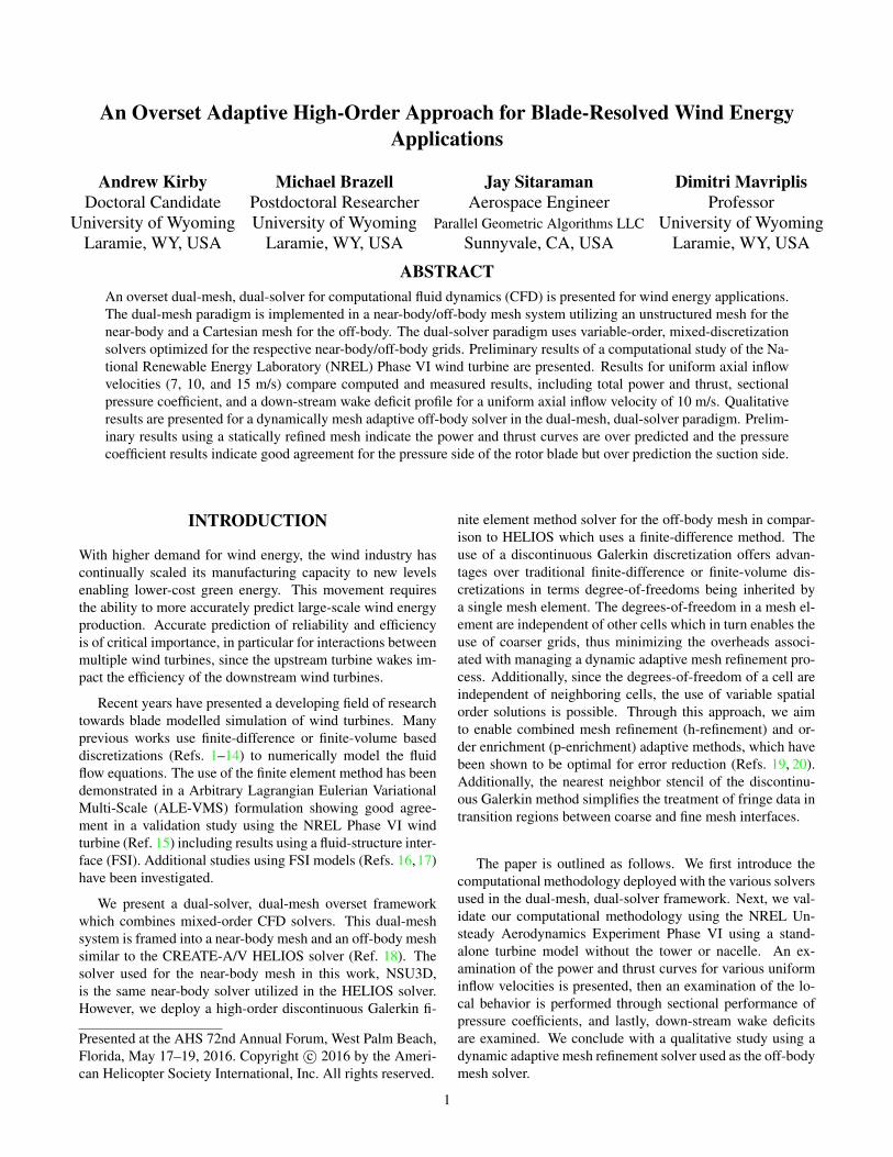
W2A2KE3D is framed in a near-body/off-body mesh sys-tem utilizing an unstructured mesh for the near-body meshand a structured mesh for the off-body mesh as illustrated inFigure 1. The current framework allows for interchangeablesolvers and mesh systems. Table 1 displays the solvers andtheir temporal discretizations. Table 2 displays the spatial dis-cretization and mesh characteristics. Descriptions of the flowsolvers are presented hereafter.
Table 1. W2A2KE3D Flow Solver Temporal SchemesSolver Temporal DiscretizationsNSU3D (Ref. 22) BDF2, BDF3DG3D (Ref. 27) BDF2, RK4CartDG (Ref. 29) RK2, RK4SAMCartDG (Ref. 29) RK2, RK4
Fig. 1. Near-body/off-body mesh system utilized in theW2A2KE3D solver.
SOLVERS
Near-Body Unstructured Mesh Solver: NSU3D
The near-body unstructured mesh solver used in the presentwork is NSU3D (Refs. 22–24). NSU3D is a well-establishedvertex-centered finite-volume solver for mixed element un-structured meshes. NSU3D solves the Unsteady ReynoldsAveraged Navier-Stokes (URANS) equations through a multi-grid technique. It has second-order spatial discretization usingleast-squares gradient reconstruction. NSU3D has second-
and third-order accurate temporal discretizations via the im-plicit BDF2 and BDF3 schemes, respectively. The solver hasautomatic agglomeration multigrid and line implicit precondi-tioning for solution acceleration. NSU3D has been thoroughlyvalidated and verified through regular participation as a mem-ber of the AIAA High Lift Prediction Workshop (Ref. 25) andthe AIAA Drag Prediction Workshop (Ref. 26).
Near-Body Unstructured Mesh Solver: DG3D
A second near-body unstructured solver in the W2A2KE3Dsolver collection is DG3D. DG3D is a high-order, mixed-and curved element unstructured mesh solver (Refs. 27, 28)capable of spatial order-of-accuracy ranging from first- tosixth- order. It is developed based on the discontinuousGalerkin (DG) finite element method (FEM) for the compress-ible Navier-Stokes equations. The temporal derivative is han-dled through an explicit Runge-Kutta method or an implicitBDF2 scheme. DG3D has been successfully applied to hy-personic problems, turbulent flow problems, full aircraft sim-ulation, the Taylor-Green Vortex problem, and overset simu-lations (Ref. 21).
Off-Body Static Structured Mesh Solver: CartDG
CartDG is a high-order block Cartesian discontinuousGalerkin finite element method based compressible Navier-Stokes solver (Ref. 29). CartDG is a nodal, collocated, tensor-product basis formulation. It is developed to handle an arbi-trary spatial order-of-accuracy and has explicit time-steppingof second- and fourth-orders via the Runge-Kutta method.CartDG in stand-alone mode has been demonstrated for vari-ous viscous and inviscid problems, notably the Taylor-GreenVortex problem (Refs. 30, 31) and the diagonally lid-drivencavity problem (Ref. 32).
Off-Body Structured AMR Solver: SAMCartDG
The off-body adaptive structured mesh solver SAMCartDG isthe adaptive mesh refinement (AMR) extension of the CartDGsolver. SAMCartDG is implemented into the StructuredAdaptive Mesh Refinement Applications Interface (Refs. 34,35) (SAMRAI) developed at Lawrence Livermore NationalLaboratory. SAMRAI is a patch based AMR system of prop-erly nested refinement levels containing logically rectangulargrid blocks. Grid generation and structure, parallel commu-nication, and load balancing of SAMCartDG are handled bythe SAMRAI infrastructure. SAMRAI allows for redistribu-tion of restart solutions through file I/O. As a solution evolvesover time, more features may need to be tracked increasing thenumber of elements in the solution. Between restart intervalsof solutions, SAMCartDG is able to redistribute its solutionto a different number of processors if needed. On regriddingintervals, cells are tagged for refinement using feature-baseddetection. Tagging algorithms in SAMCartDG are based ondensity gradient, vorticity magnitude, and non-dimensionalQ-Criterion (Ref. 36).
2
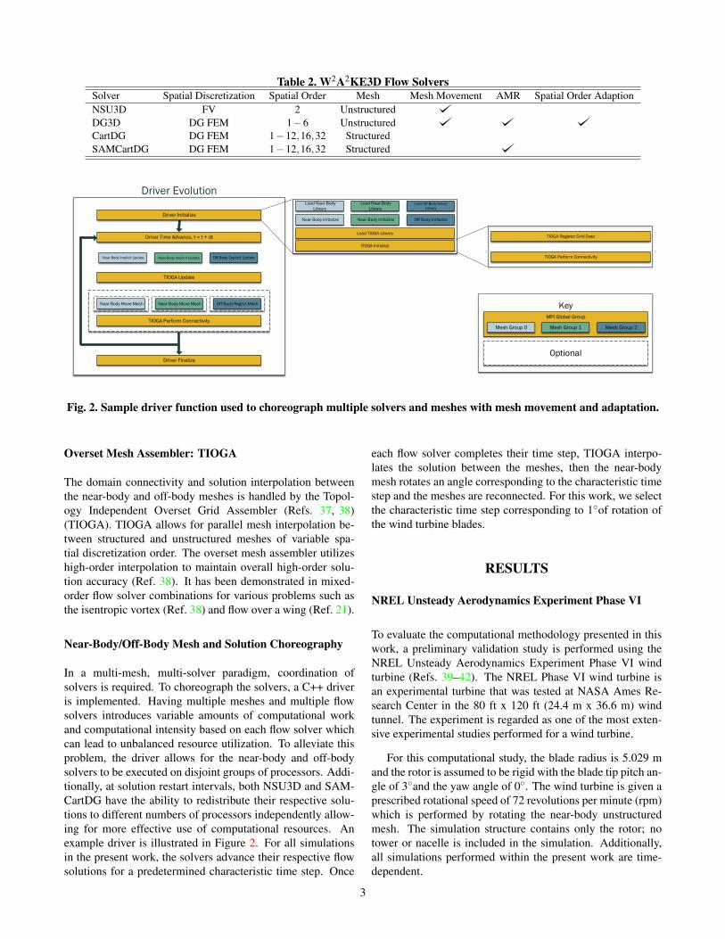
Table 2. W2A2KE3D Flow SolversSolver Spatial Discretization Spatial Order Mesh Mesh Movement AMR Spatial Order AdaptionNSU3D FV 2 UnstructuredDG3D DG FEM 1−6 UnstructuredCartDG DG FEM 1−12,16,32 StructuredSAMCartDG DG FEM 1−12,16,32 Structured
KeyMPI Global Group
Driver Initialize
Load Near-Body Library
Load Near-Body Library
Load Off-Body Solver Library
Mesh Group 0 Mesh Group 1 Mesh Group 2
Near-Body Initialize Near-Body Initialize Off-Body Initialize
Load TIOGA LibraryTIOGA Register Grid Data
TIOGA Perform Connectivity
Driver Time Advance, t = t + dt
Optional
Near-Body Implicit Update Near-Body Implicit Update Off-Body Explicit Update
TIOGA Update
TIOGA Perform Connectivity
Driver Evolution
Driver Finalize
Near-Body Move Mesh Near-Body Move Mesh Off-Body Regrid Mesh
TIOGA Initialize
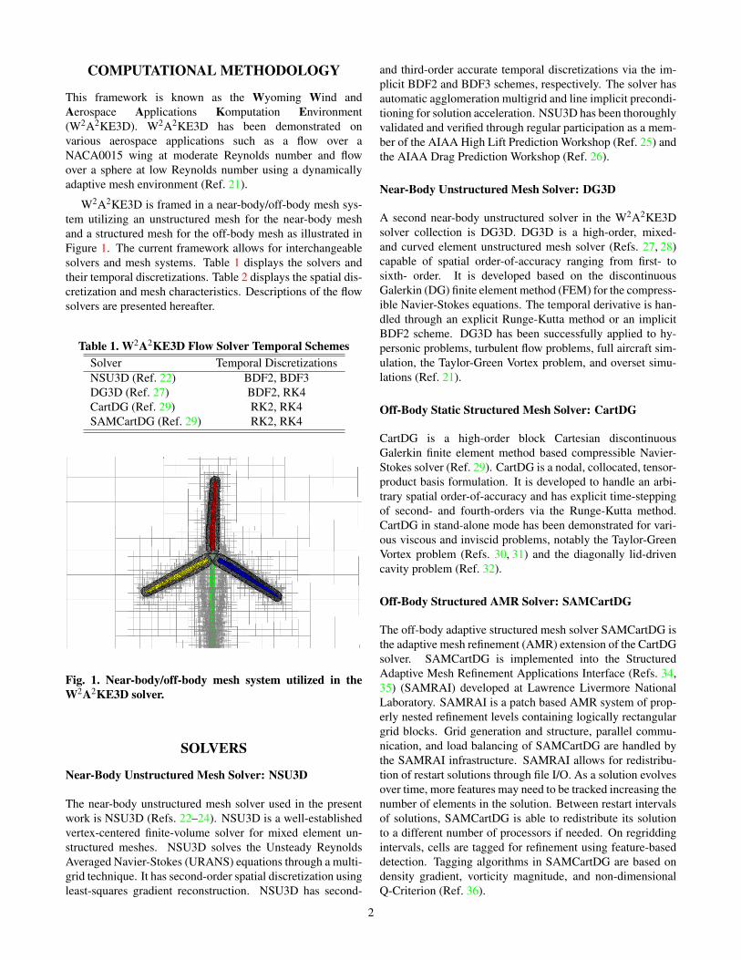
Fig. 2. Sample driver function used to choreograph multiple solvers and meshes with mesh movement and adaptation.
Overset Mesh Assembler: TIOGA
The domain connectivity and solution interpolation betweenthe near-body and off-body meshes is handled by the Topol-ogy Independent Overset Grid Assembler (Refs. 37, 38)(TIOGA). TIOGA allows for parallel mesh interpolation be-tween structured and unstructured meshes of variable spa-tial discretization order. The overset mesh assembler utilizeshigh-order interpolation to maintain overall high-order solu-tion accuracy (Ref. 38). It has been demonstrated in mixed-order flow solver combinations for various problems such asthe isentropic vortex (Ref. 38) and flow over a wing (Ref. 21).
Near-Body/Off-Body Mesh and Solution Choreography
In a multi-mesh, multi-solver paradigm, coordination ofsolvers is required. To choreograph the solvers, a C++ driveris implemented. Having multiple meshes and multiple flowsolvers introduces variable amounts of computational workand computational intensity based on each flow solver whichcan lead to unbalanced resource utilization. To alleviate thisproblem, the driver allows for the near-body and off-bodysolvers to be executed on disjoint groups of processors. Addi-tionally, at solution restart intervals, both NSU3D and SAM-CartDG have the ability to redistribute their respective solu-tions to different numbers of processors independently allow-ing for more effective use of computational resources. Anexample driver is illustrated in Figure 2. For all simulationsin the present work, the solvers advance their respective flowsolutions for a predetermined characteristic time step. Once
each flow solver completes their time step, TIOGA interpo-lates the solution between the meshes, then the near-bodymesh rotates an angle corresponding to the characteristic timestep and the meshes are reconnected. For this work, we selectthe characteristic time step corresponding to 1◦of rotation ofthe wind turbine blades.
RESULTS
NREL Unsteady Aerodynamics Experiment Phase VI
To evaluate the computational methodology presented in thiswork, a preliminary validation study is performed using theNREL Unsteady Aerodynamics Experiment Phase VI windturbine (Refs. 39–42). The NREL Phase VI wind turbine isan experimental turbine that was tested at NASA Ames Re-search Center in the 80 ft x 120 ft (24.4 m x 36.6 m) windtunnel. The experiment is regarded as one of the most exten-sive experimental studies performed for a wind turbine.
For this computational study, the blade radius is 5.029 mand the rotor is assumed to be rigid with the blade tip pitch an-gle of 3◦and the yaw angle of 0◦. The wind turbine is given aprescribed rotational speed of 72 revolutions per minute (rpm)which is performed by rotating the near-body unstructuredmesh. The simulation structure contains only the rotor; notower or nacelle is included in the simulation. Additionally,all simulations performed within the present work are time-dependent.
3
CREATE-A/V HELIOS Solver and FLOWYO Solver
In addition to experimental data comparison for the Phase VIwind turbine, we compare results with the CREATE-A/V HE-LIOS solver (Refs. 18, 43–45). HELIOS is an overset adap-tive mesh solver for the Reynolds Averaged Navier-Stokes(RANS) equations. It uses NSU3D as the near-body solverand an adaptive fifth-order accurate finite-difference methodwith third-order accurate temporal discretization. HELIOShas been extensively validated using problems from aerospacesuch as forward-flight helicopters (Ref. 43) and from the windenergy field (Ref. 46). Specifically, we compare numericalresults from Gundling et. al (Ref. 17). We note that the HE-LIOS solver performed steady, non-inertial simulations for thePhase VI wind turbine. The near-body and off-body mesheswere connected one time through an overset process.
Further, we compare results to FLOWYO (Refs. 17, 47).FLOWYO is a RANS and Large Eddy Simulation (LES)solver.
Fig. 3. Unstructured surface mesh of the NREL Phase VIwind turbine blade.
Near-Body Mesh and Solver Set-up
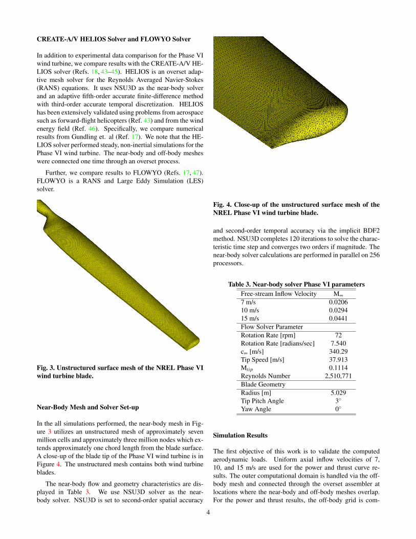
In the all simulations performed, the near-body mesh in Fig-ure 3 utilizes an unstructured mesh of approximately sevenmillion cells and approximately three million nodes which ex-tends approximately one chord length from the blade surface.A close-up of the blade tip of the Phase VI wind turbine is inFigure 4. The unstructured mesh contains both wind turbineblades.
The near-body flow and geometry characteristics are dis-played in Table 3. We use NSU3D solver as the near-body solver. NSU3D is set to second-order spatial accuracy
Fig. 4. Close-up of the unstructured surface mesh of theNREL Phase VI wind turbine blade.
and second-order temporal accuracy via the implicit BDF2method. NSU3D completes 120 iterations to solve the charac-teristic time step and converges two orders if magnitude. Thenear-body solver calculations are performed in parallel on 256processors.
Table 3. Near-body solver Phase VI parametersFree-stream Inflow Velocity M∞
7 m/s 0.020610 m/s 0.029415 m/s 0.0441Flow Solver ParameterRotation Rate [rpm] 72Rotation Rate [radians/sec] 7.540c∞ [m/s] 340.29Tip Speed [m/s] 37.913Mtip 0.1114Reynolds Number 2,510,771Blade GeometryRadius [m] 5.029Tip Pitch Angle 3◦
Yaw Angle 0◦
Simulation Results
The first objective of this work is to validate the computedaerodynamic loads. Uniform axial inflow velocities of 7,10, and 15 m/s are used for the power and thrust curve re-sults. The outer computational domain is handled via the off-body mesh and connected through the overset assembler atlocations where the near-body and off-body meshes overlap.For the power and thrust results, the off-body grid is com-
4

5 10 15 20 252
4
6
8
10
12
14
Wind Speed [m/s]
Pow
er [k
W]
ExperimentHelios
W2A2KE3D
5 10 15 20 25500
1000
1500
2000
2500
3000
3500
4000
4500
5000
Wind Speed [m/s]
Thr
ust [
N]
ExperimentHelios
W2A2KE3D
Fig. 5. Power and thrust curves for W2A2KE3D and HELIOS versus NREL experimental data.
0 200 400 600 800 1000 1200 1400500
1000
1500
2000
2500
3000
3500
4000
4500
time steps
Thr
ust [
N]
15 m/s
10 m/s
7 m/s
InstantaneousMoving Average
Fig. 6. Thrust convergence for inflow velocities 7, 10, and15 m/s.
posed of a refined mesh of physical domain (−7.5m,7.5m)x (−7.5m,7.5m) x (−3m,27m) using 192 elements in the x-direction, 192 elements in the y-direction, and 600 elementsin the z-direction, respectively. The off-body solver is cho-sen to be CartDG which uses a second-order accurate spatialdiscretization of the inviscid Euler equations and a second-order accurate temporal discretization. We note the computa-tional solution is time-dependent. At second-order spatial ac-curacy, the off-body solution contains approximately 177 mil-lion degrees-of-freedom (DOF) per equation which equates toapproximately 885 million unknowns per Runge-Kutta stage.CartDG uses 8192 processors to solve the off-body calcula-tions. The solvers are able to achieve approximately 1200◦ofrotation in a 12 hour compute window.
Power and thrust curves for W2A2KE3D and HELIOS areshown in Figure 5 along with the NREL experimental data.Thrust convergence history is displayed in Figure 6. The
power and thrust curves represent the integrated effect of theaerodynamic loads acting on the rotor blades. As indicated inFigure 6, convergence of aerodynamic loading is achieved forall the wind speeds. Larger number of time steps are requiredto obtain converged forces at higher wind speeds owing to thepresence of flow separation.
To better examine the local behavior, we investigate thepressure coefficient over the blade surface at various sectionallocations on the computational mesh used for the power andthrust curve analysis. The sectional pressure coefficient Cp iscomputed as
Cp =p− p∞
12 ρ∞
(U2
∞ +(rω)2) (1)
where U∞ is the free-stream inflow speed, ω is the rotationspeed, and r is the sectional radius. The off-body mesh ischosen to be the same as the mesh used in the power and thrustresults. Figure 7 shows the surface coefficient of pressure at10 m/s inflow velocity.
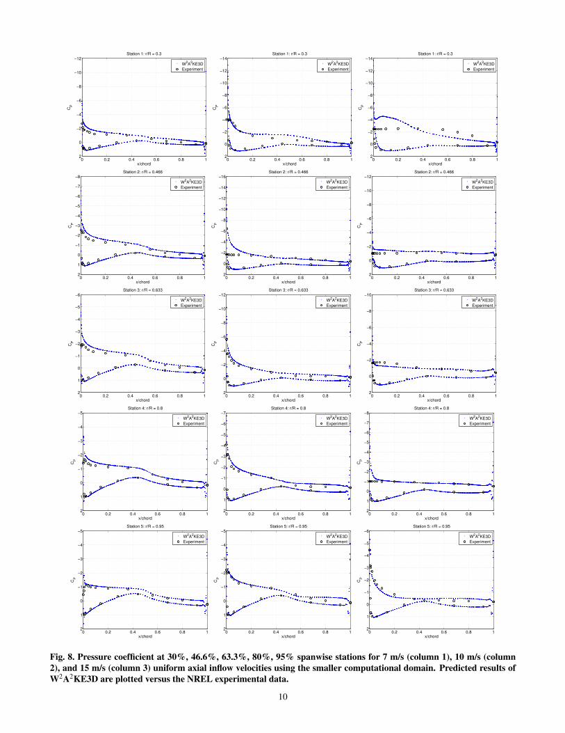
Figure 8 shows the pressure coefficient at30%,46.6%,63.3%,80% and 95% spanwise stations ofthe blade for 7, 10, and 15 m/s uniform inflow velocities. Inall inflow velocity cases at all sectional locations, the coef-ficient of pressure values on the pressure side of the turbineblade are fairly well predicted. The S809 airfoil sectionused shows alleviation of the adverse pressure gradients atmid-chord regions, which manifests as an inflexion in thepressure coefficient curves. The current analysis shows goodagreement with data in prediction of this pattern. However,notice that in the 7 and 10 m/s cases, the coefficient of pres-sure on the suction side is higher than the experimental valuesat all sectional locations. Additionally, notable discrepanciesare found at 10 m/s for the location r/R = 46.6%, and for15 m/s at r/R = 30%. Similar inconsistencies are found inother researchers results (Refs. 4, 5, 13, 15) and is thoughtto be caused by inaccuracies in prediction of separated
5

Fig. 7. Surface plots of the coefficient of pressure for inflowvelocity of 10 m/s.
flow because of deficiencies in modeling laminar/turbulenttransition.
A simulation is performed to analyze the wind wake veloc-ity deficit. The computational domain is (−11.25m,11.25m)x (−11.25m,11.25m) x (−5m,55m) with 288 elements in thex-direction, 288 elements in the y-direction, and 1200 ele-ments in the z-direction, respectively.
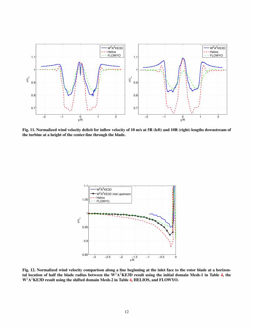
Figure 10 demonstrates the normalized wind velocitydeficit along a line from the inlet of the domain to the out-let of the domain at a horizontal location of half a blade ra-dius for inflow velocity of 10 m/s. Figure 11 demonstratesthe normalized wind velocity wake deficits at 5 and 10 ra-dius lengths downstream of the turbine blade. Notice the nor-malized velocity at the boundary interfaces in Figure 11; thevalues of the normalized velocity at the boundary interfacesshould asymptote to a value of one representing free-stream.Typically an influence is observed when a computational do-main is too small.
To compare the meshes used in the previous results, weincrease the size and shift the computational domain to phys-ical dimensions of (−11.25m,11.25m) x (−11.25m,11.25m)x (−20m,40m) with 288 elements in the x-direction, 288 ele-ments in the y-direction, and 1200 elements in the z-direction,respectively. Notice the inlet boundary is now approximatelyfour blade radius lengths away from the rotor blade. We listthe mesh used in the previous results in Table 4 as Mesh-1 along side the larger, shifted computational mesh listed asMesh-2. The larger computational domain increases the prob-lem to nearly 800 million DOF per conservative variable forsecond-order spatial accuracy which equates to approximately4 billion unknowns per Runge-Kutta stage. Approximately1000◦of rotation is achieved in a 12 hour simulation cam-paign. Figure 12 shows the inflow velocities coming inboardto the rotor blade. Notice that for the larger computational
domain, the inboard velocity is closer to the FLOWYO andHELIOS results. However, the inlet velocity hasn’t droppedto the same velocity as the HELIOS results.
Table 4. Wake Deficit Profile MeshesDomain Mesh-1 Mesh-2xlo -11.25 -11.25xhi 11.25 11.25ylo -11.25 -11.25yhi 11.25 11.25zlo -5.0 55.0zhi -20.0 40.0ElementsNx 288 288Ny 288 288Nz 1200 1200
Figure 13 shows the pressure coefficients of the smallerdomain compared to the pressure coefficients of the larger do-main at a free-stream inflow velocity of 10 m/s. Results areslightly improved when using the larger computational do-main for the suction side of the rotor blade. These slight im-provements reflect the positive impact of using a larger com-putational domain.
Figure 14 illustrates the difference between the two meshesfor the normalized wind velocity deficit profiles along a linefrom the inlet of the domain to the outlet of the domain at ahorizontal location of half the blade radius for inflow velocityof 10 m/s. Figure 15 demonstrates the normalized wind veloc-ity deficit comparison at five blade radius lengths downstreamof the turbine blade. We see a significant improvement overthe computational results of Mesh-1 by using Mesh-2. Thisconfirms the hypothesis that the domain used in the initial re-sults has the inlet boundary close to the rotor blade. Both ofthe present results give a higher wind speed velocity comparedto the HELIOS numerical result. However, both W2A2KE3Dresults do give better solutions than the FLOWYO (Ref. 17)result. Notice the normalized velocity at the boundary inter-faces in Figure 15; the values of the normalized velocity atthe boundary interfaces should asymptote to a value of onerepresenting free-stream.
DYNAMIC ADAPTIVE MESH RESULTS
Computations that use a moving near-body mesh system inan AMR hierarchy is an upcoming capability of W2A2KE3Dinfrastructure and only preliminary results are available atthis time. The adaptive solution is computed using acomputational domain of (−49m,49m) x (−49m,49m) x(−50m,202m). Figure 16 shows the adaptive mesh solutionusing approximately five million elements.
Further reduction in the total elements is obtained via anoverset mesh resolution matching algorithm. The oversetmesh assembler requires the near-body and off-body meshesbe of the same approximate size in the overlap regions. Tosave elements in the off-body mesh, the mesh is adapted to
6
a set of outer boundary grid points provided by the trimmednear-body unstructured mesh. The geometric adaption of theoff-body grid refines to a prescribed reference length providedfor each near-body grid boundary point. Figure 16 showsthe off-body mesh geometrically and solution adapted to theNREL Phase VI blade.
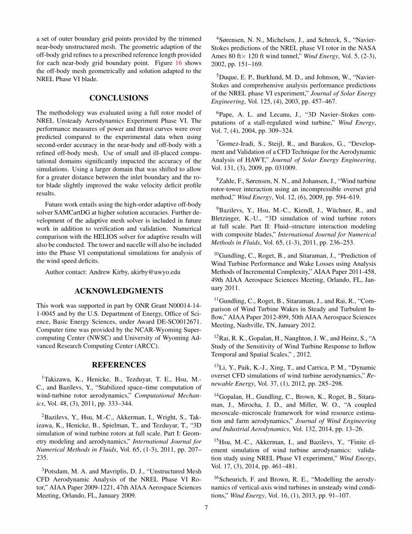
CONCLUSIONS
The methodology was evaluated using a full rotor model ofNREL Unsteady Aerodynamics Experiment Phase VI. Theperformance measures of power and thrust curves were overpredicted compared to the experimental data when usingsecond-order accuracy in the near-body and off-body with arefined off-body mesh. Use of small and ill-placed compu-tational domains significantly impacted the accuracy of thesimulations. Using a larger domain that was shifted to allowfor a greater distance between the inlet boundary and the ro-tor blade slightly improved the wake velocity deficit profileresults.
Future work entails using the high-order adaptive off-bodysolver SAMCartDG at higher solution accuracies. Further de-velopment of the adaptive mesh solver is included in futurework in addition to verification and validation. Numericalcomparison with the HELIOS solver for adaptive results willalso be conducted. The tower and nacelle will also be includedinto the Phase VI computational simulations for analysis ofthe wind speed deficits.
Author contact: Andrew Kirby, [email protected]
ACKNOWLEDGMENTS
This work was supported in part by ONR Grant N00014-14-1-0045 and by the U.S. Department of Energy, Office of Sci-ence, Basic Energy Sciences, under Award DE-SC0012671.Computer time was provided by the NCAR-Wyoming Super-computing Center (NWSC) and University of Wyoming Ad-vanced Research Computing Center (ARCC).
REFERENCES1Takizawa, K., Henicke, B., Tezduyar, T. E., Hsu, M.-
C., and Bazilevs, Y., “Stabilized space–time computation ofwind-turbine rotor aerodynamics,” Computational Mechan-ics, Vol. 48, (3), 2011, pp. 333–344.
2Bazilevs, Y., Hsu, M.-C., Akkerman, I., Wright, S., Tak-izawa, K., Henicke, B., Spielman, T., and Tezduyar, T., “3Dsimulation of wind turbine rotors at full scale. Part I: Geom-etry modeling and aerodynamics,” International Journal forNumerical Methods in Fluids, Vol. 65, (1-3), 2011, pp. 207–235.
3Potsdam, M. A. and Mavriplis, D. J., “Unstructured MeshCFD Aerodynamic Analysis of the NREL Phase VI Ro-tor,” AIAA Paper 2009-1221, 47th AIAA Aerospace SciencesMeeting, Orlando, FL, January 2009.
4Sørensen, N. N., Michelsen, J., and Schreck, S., “Navier-Stokes predictions of the NREL phase VI rotor in the NASAAmes 80 ft× 120 ft wind tunnel,” Wind Energy, Vol. 5, (2-3),2002, pp. 151–169.
5Duque, E. P., Burklund, M. D., and Johnson, W., “Navier-Stokes and comprehensive analysis performance predictionsof the NREL phase VI experiment,” Journal of Solar EnergyEngineering, Vol. 125, (4), 2003, pp. 457–467.
6Pape, A. L. and Lecanu, J., “3D Navier–Stokes com-putations of a stall-regulated wind turbine,” Wind Energy,Vol. 7, (4), 2004, pp. 309–324.
7Gomez-Iradi, S., Steijl, R., and Barakos, G., “Develop-ment and Validation of a CFD Technique for the AerodynamicAnalysis of HAWT,” Journal of Solar Energy Engineering,Vol. 131, (3), 2009, pp. 031009.
8Zahle, F., Sørensen, N. N., and Johansen, J., “Wind turbinerotor-tower interaction using an incompressible overset gridmethod,” Wind Energy, Vol. 12, (6), 2009, pp. 594–619.
9Bazilevs, Y., Hsu, M.-C., Kiendl, J., Wuchner, R., andBletzinger, K.-U., “3D simulation of wind turbine rotorsat full scale. Part II: Fluid–structure interaction modelingwith composite blades,” International Journal for NumericalMethods in Fluids, Vol. 65, (1-3), 2011, pp. 236–253.
10Gundling, C., Roget, B., and Sitaraman, J., “Prediction ofWind Turbine Performance and Wake Losses using AnalysisMethods of Incremental Complexity,” AIAA Paper 2011-458,49th AIAA Aerospace Sciences Meeting, Orlando, FL, Jan-uary 2011.
11Gundling, C., Roget, B., Sitaraman, J., and Rai, R., “Com-parison of Wind Turbine Wakes in Steady and Turbulent In-flow,” AIAA Paper 2012-899, 50th AIAA Aerospace SciencesMeeting, Nashville, TN, January 2012.
12Rai, R. K., Gopalan, H., Naughton, J. W., and Heinz, S., “AStudy of the Sensitivity of Wind Turbine Response to InflowTemporal and Spatial Scales,” , 2012.
13Li, Y., Paik, K.-J., Xing, T., and Carrica, P. M., “Dynamicoverset CFD simulations of wind turbine aerodynamics,” Re-newable Energy, Vol. 37, (1), 2012, pp. 285–298.
14Gopalan, H., Gundling, C., Brown, K., Roget, B., Sitara-man, J., Mirocha, J. D., and Miller, W. O., “A coupledmesoscale–microscale framework for wind resource estima-tion and farm aerodynamics,” Journal of Wind Engineeringand Industrial Aerodynamics, Vol. 132, 2014, pp. 13–26.
15Hsu, M.-C., Akkerman, I., and Bazilevs, Y., “Finite el-ement simulation of wind turbine aerodynamics: valida-tion study using NREL Phase VI experiment,” Wind Energy,Vol. 17, (3), 2014, pp. 461–481.
16Scheurich, F. and Brown, R. E., “Modelling the aerody-namics of vertical-axis wind turbines in unsteady wind condi-tions,” Wind Energy, Vol. 16, (1), 2013, pp. 91–107.
7

17Gundling, C., Sitaraman, J., Roget, B., and Masarati, P.,“Application and validation of incrementally complex modelsfor wind turbine aerodynamics, isolated wind turbine in uni-form inflow conditions,” Wind Energy, Vol. 18, (11), 2015,pp. 1893–1916.
18Wissink, A. M., Sitaraman, J., Sankaran, V., Mavriplis,D. J., and Pulliam, T. H., “A Multi-Code Python-Based In-frastructure for Overset CFD with Adaptive Cartesian Grids,”AIAA Paper 2008-927, 46th AIAA Aerospace Sciences Meet-ing, Reno, NV, January 2008.
19Solin, P., Segeth, K., and Dolezel, I., Higher-order finiteelement methods, CRC Press, 2003.
20Burgess, N. K. and Mavriplis, D. J., “hp-Adaptive dis-continuous Galerkin solver for the Navier-Stokes equations,”AIAA Journal, Vol. 50, (12), 2012, pp. 2682–2694.
21Brazell, M. J., Kirby, A. C., Sitaraman, J., and Mavriplis,D. J., “A Multi-Solver Overset Mesh Approach for 3D MixedElement Variable Order Discretizations,” AIAA Paper 2016-2053, 54th AIAA Aerospace Sciences Meeting, San Diego,CA, January 2016.
22Mavriplis, D. J., “Results from the 3rd Drag PredictionWorkshop using the NSU3D Unstructured Mesh Solver,”AIAA Paper 2007-256, 45th AIAA Aerospace Sciences Meet-ing, Reno, NV, January 2007.
23Mavriplis, D. and Pirzadeh, S., Large-scale parallelunstructured mesh computations for 3D high-lift analy-sis, American Institute of Aeronautics and Astronautics,2015/06/01 1999.doi: 10.2514/6.1999-537
24Mavriplis, D. J., “Multigrid Strategies for Viscous FlowSolvers on Anisotropic Unstructured Meshes,” Journal ofComputational Physics, Vol. 145, (1), 1998, pp. 141–165.
25Long, M. and Mavriplis, D., “NSU3D Results for the FirstAIAA High Lift Prediction Workshop,” AIAA Paper 2011-0863, 49th AIAA Aerospace Sciences Meeting, Orlando, FL,January 2011.
26Mavriplis, D. J., “Third Drag Prediction Workshop ResultsUsing the NSU3D Unstructured Mesh Solver,” Journal of Air-craft, Vol. 45, (3), 2015/06/01 2008, pp. 750–761.doi: 10.2514/1.29828
27Brazell, M. J. and Mavriplis, D. J., “3D Mixed ElementDiscontinuous Galerkin with Shock Capturing,” AIAA Pa-per 2013-2855, 21st AIAA CFD Conference, San Diego, CA,June 2013.
28Brazell, M. J. and Mavriplis, D. J., “High-Order Discon-tinuous Galerkin Mesh Resolved Turbulent Flow Simulationsof a NACA 0012 Airfoil (Invited),” AIAA Paper 2015-1529,53rd AIAA Aerospace Sciences Meeting, Kissimmee, FL,January 2015.
29Kirby, A. C., Mavriplis, D. J., and Wissink, A. M., “AnAdaptive Explicit 3D Discontinuous Galerkin Solver for Un-steady Problems,” AIAA Paper 2015-3046, 22nd AIAA Com-putational Fluid Dynamics Conference, Dallas, TX, June2015.
30Taylor, G. and Green, A., “Large Ones,” Proceedings of theRoyal Society of London. Series A, Mathematical and Physi-cal Sciences, Vol. 158, (895), 1937, pp. 499–521.
31Brachet, M., “Direct simulation of three-dimensional tur-bulence in the Taylor-Green vortex,” Fluid Dynamics Re-search, Vol. 8, (1), 1991, pp. 1–8.
32Povitsky, A., “High-Incidence 3-D Lid-Driven CavityFlow,” AIAA Paper 2001-2847, 15th AIAA ComputationalFluid Dynamics Conference, Anaheim, CA, June 2001.
33National Center for Atmospheric Research, Boulder, CO,Yellowstone: IBM iDataPlex System (Climate SimulationLaboratory), http://n2t.net/ark:/85065/d7wd3xhc, 2012.
34Hornung, R. D., Wissink, A. M., and Kohn, S. R., “Man-aging complex data and geometry in parallel structured AMRapplications,” Engineering with Computers, Vol. 22, (3-4),2006, pp. 181–195.
35Gunney, B. T., Wissink, A. M., and Hysom, D. A., “Parallelclustering algorithms for structured AMR,” Journal of Paral-lel and Distributed Computing, Vol. 66, (11), 2006, pp. 1419–1430.
36Kamkar, S., Jameson, A. J., and Wissink, A. M., “Au-tomated Grid Refinement Using Feature Detection,” AIAAPaper 2009-1496, 47th AIAA Aerosciences Conference, Or-lando, FL, January 2009.
37Roget, B. and Sitaraman, J., “Robust and efficient oversetgrid assembly for partitioned unstructured meshes,” Journalof Computational Physics, Vol. 260, 2014, pp. 1–24.
38Brazell, M. J., Mavriplis, D. J., and Sitaraman, J., “AnOverset Mesh Approach for 3D Mixed Element High Or-der Discretizations,” AIAA Paper 2015-1739, 53rd AIAAAerospace Sciences Meeting, Kissimmee, FL, January 2014.
39Hand, M. M., Simms, D., Fingersh, L., Jager, D., Cotrell,J., Schreck, S., and Larwood, S., Unsteady aerodynamics ex-periment phase VI: wind tunnel test configurations and avail-able data campaigns, National Renewable Energy Labora-tory, Golden, Colorado, USA, 2001.
40Simms, D. A., Schreck, S., Hand, M., and Fingersh, L.,NREL unsteady aerodynamics experiment in the NASA-Ameswind tunnel: a comparison of predictions to measurements,National Renewable Energy Laboratory Golden, CO, USA,2001.
41Schreck, S., “The NREL full-scale wind tunnel experimentIntroduction to the special issue,” Wind Energy, Vol. 5, (2-3),2002, pp. 77–84.
8

42Fingersh, L. J., Simms, D., Hand, M., Jager, D., Cotrell,J., Robinson, M., Schreck, S., and Larwood, S., “Wind Tun-nel Testing of NRELs Unsteady Aerodynamics Experiment,”AIAA Paper 2001-35, 20th ASME Wind Energy Symposiumand the 39th Aerospace Sciences Meeting, Reno, NV, 2001.
43Sankaran, V., Sitaraman, J., Wissink, A., Datta, A., Jayara-man, B., Potsdam, M., Mavriplis, D., Yang, Z., OBrien, D.,Saberi, H., et al., “Application of the Helios ComputationalPlatform to Rotorcraft Flowfields,” AIAA Paper 2010-1230,48th AIAA Aerospace Meeting, Orlando, FL, 2010.
44Wissink, A., Jayaraman, B., Datta, A., Sitaraman, J., Pots-dam, M., Kamkar, S., Mavriplis, D., Yang, Z., Jain, R.,Lim, J., et al., “Capability Enhancements in Version 3 ofthe Helios High-Fidelity Rotorcraft Simulation Code,” AIAAPaper 2012-0713, 50th AIAA Aerospace Science Meeting,Nashville, TN, 2012.
45Wissink, A. M., Kamkar, S., Pulliam, T. H., Sitaraman, J.,and Sankaran, V., “Cartesian Adaptive Mesh Refinement forRotorcraft Wake Resolution,” AIAA Paper 2010-4554, 28thApplied Aerodynamics Conference, Chicago, IL, 2010.
46Sitaraman, J., Mavriplis, D., and Duque, E. P., “Wind farmsimulations using a full rotor model for wind turbines,” Pro-ceedings of the AIAA SciTech 2014 Meeting, National Har-bor, MD, 2014.
47Gundling, C. H., Development and application of incre-mentally complex tools for wind turbine aerodynamics, 2013.
9
0 0.2 0.4 0.6 0.8 1
−12
−10
−8
−6
−4
−2
0
2
x/chord
CP
Station 1: r/R = 0.3
W2A
2KE3D
Experiment
0 0.2 0.4 0.6 0.8 1
−14
−12
−10
−8
−6
−4
−2
0
2
x/chord
CP
Station 1: r/R = 0.3
W2A
2KE3D
Experiment
0 0.2 0.4 0.6 0.8 1
−14
−12
−10
−8
−6
−4
−2
0
2
x/chord
CP
Station 1: r/R = 0.3
W2A
2KE3D
Experiment
0 0.2 0.4 0.6 0.8 1
−8
−7
−6
−5
−4
−3
−2
−1
0
1
2
x/chord
CP
Station 2: r/R = 0.466
W2A
2KE3D
Experiment
0 0.2 0.4 0.6 0.8 1
−16
−14
−12
−10
−8
−6
−4
−2
0
2
x/chord
CP
Station 2: r/R = 0.466
W2A
2KE3D
Experiment
0 0.2 0.4 0.6 0.8 1
−12
−10
−8
−6
−4
−2
0
2
x/chord
CP
Station 2: r/R = 0.466
W2A
2KE3D
Experiment
0 0.2 0.4 0.6 0.8 1
−6
−5
−4
−3
−2
−1
0
1
2
x/chord
CP
Station 3: r/R = 0.633
W2A
2KE3D
Experiment
0 0.2 0.4 0.6 0.8 1
−12
−10
−8
−6
−4
−2
0
2
x/chord
CP
Station 3: r/R = 0.633
W2A
2KE3D
Experiment
0 0.2 0.4 0.6 0.8 1
−10
−8
−6
−4
−2
0
2
x/chord
CP
Station 3: r/R = 0.633
W2A
2KE3D
Experiment
0 0.2 0.4 0.6 0.8 1
−5
−4
−3
−2
−1
0
1
2
x/chord
CP
Station 4: r/R = 0.8
W2A
2KE3D
Experiment
0 0.2 0.4 0.6 0.8 1
−7
−6
−5
−4
−3
−2
−1
0
1
2
x/chord
CP
Station 4: r/R = 0.8
W2A
2KE3D
Experiment
0 0.2 0.4 0.6 0.8 1
−8
−7
−6
−5
−4
−3
−2
−1
0
1
2
x/chord
CP
Station 4: r/R = 0.8
W2A
2KE3D
Experiment
0 0.2 0.4 0.6 0.8 1
−5
−4
−3
−2
−1
0
1
2
x/chord
CP
Station 5: r/R = 0.95
W2A
2KE3D
Experiment
0 0.2 0.4 0.6 0.8 1
−5
−4
−3
−2
−1
0
1
2
x/chord
CP
Station 5: r/R = 0.95
W2A
2KE3D
Experiment
0 0.2 0.4 0.6 0.8 1
−6
−5
−4
−3
−2
−1
0
1
2
x/chord
CP
Station 5: r/R = 0.95
W2A
2KE3D
Experiment
Fig. 8. Pressure coefficient at 30%, 46.6%, 63.3%, 80%, 95% spanwise stations for 7 m/s (column 1), 10 m/s (column2), and 15 m/s (column 3) uniform axial inflow velocities using the smaller computational domain. Predicted results ofW2A2KE3D are plotted versus the NREL experimental data.
10

Fig. 9. Wind velocity contour of Phase VI wind turbine colored by density.
−2 0 2 4 6 8 10 120.5
0.6
0.7
0.8
0.9
1
1.1
z/R
u/u
∞
W2A
2KE3D
Helios
FLOWYO
Fig. 10. Normalized wind velocity deficit along a line from the domain inlet to the domain outlet at a horizontal locationof half the blade radius for inflow velocity of 10 m/s.
11
−2 −1 0 1 2
0.7
0.8
0.9
1
1.1
y/R
u/u
∞
W2A
2KE3D
Helios
FLOWYO
−2 −1 0 1 2
0.7
0.8
0.9
1
1.1
y/R
u/u
∞
W2A
2KE3D
Helios
FLOWYO
Fig. 11. Normalized wind velocity deficit for inflow velocity of 10 m/s at 5R (left) and 10R (right) lengths downstream ofthe turbine at a height of the center-line through the blade.
−3 −2.5 −2 −1.5 −1 −0.5 00.85
0.9
0.95
1
1.05
1.1
z/R
u/u
∞
W2A
2KE3D
W2A
2KE3D inlet upstream
Helios
FLOWYO
Fig. 12. Normalized wind velocity comparison along a line beginning at the inlet face to the rotor blade at a horizon-tal location of half the blade radius between the W2A2KE3D result using the initial domain Mesh-1 in Table 4, theW2A2KE3D result using the shifted domain Mesh-2 in Table 4, HELIOS, and FLOWYO.
12

0 0.2 0.4 0.6 0.8 1
−14
−12
−10
−8
−6
−4
−2
0
2
x/chord
CP
Station 1: r/R = 0.3
W2A
2KE3D
W2A
2KE3D upstream
Experiment
0 0.2 0.4 0.6 0.8 1
−16
−14
−12
−10
−8
−6
−4
−2
0
2
x/chord
CP
Station 2: r/R = 0.466
W2A
2KE3D
W2A
2KE3D upstream
Experiment
0 0.2 0.4 0.6 0.8 1
−12
−10
−8
−6
−4
−2
0
2
x/chord
CP
Station 3: r/R = 0.633
W2A
2KE3D
W2A
2KE3D upstream
Experiment
0 0.2 0.4 0.6 0.8 1
−7
−6
−5
−4
−3
−2
−1
0
1
2
x/chord
CP
Station 4: r/R = 0.8
W2A
2KE3D
W2A
2KE3D upstream
Experiment
0 0.2 0.4 0.6 0.8 1
−5
−4
−3
−2
−1
0
1
2
x/chord
CP
Station 5: r/R = 0.95
W2A
2KE3D
W2A
2KE3D upstream
Experiment
Fig. 13. Pressure coefficient comparisons at 30%, 46.6%, 63.3%, 80%, 95% spanwise stations for free-stream inflowvelocities of 10 m/s using a smaller computational domain and a larger computational domain.
−2 0 2 4 6 8 10 120.5
0.6
0.7
0.8
0.9
1
1.1
z/R
u/u
∞
W2A
2KE3D
W2A
2KE3D upstream inlet
Helios
FLOWYO
Fig. 14. Normalized wind velocity deficit along a line from the domain inlet to the domain outlet at a horizontal locationof half the blade radius for inflow velocity of 10 m/s. The blue line is the solution using Mesh-1 from Table 4 and theblack line with circle markers indicates the solution using Mesh-2 in Table 4.
13

−2 −1 0 1 2
0.7
0.8
0.9
1
1.1
1.2
y/R
u/u
∞
W2A
2KE3D
W2A
2KE3D upstream inlet
Helios
FLOWYO
Fig. 15. Normalized wind velocity deficit for inflow velocity of 10 m/s at 5R (left) and 10R (right) lengths downstream ofthe turbine at a height of the center-line through the blade. The blue line is the solution using Mesh-1 from Table 4 andthe black line with circle markers indicates the solution using Mesh-2 in Table 4.
Fig. 16. Adaptive mesh solution using geometric and solution feature based adaption in SAMCartDG.
14