An Overview of Diagrammatic Notation in

Physics

John Selby

April 22, 2014

Abstract

This review looks at the development of new techniques in physics inwhich diagrams take a central role, both as an intuitive aid in understand-ing the world but also as a powerful tool for performing calculations. Inthe first section we look at the historic development of these ideas, in thesecond we then take a pragmatic approach and show how they can beused to vastly speed up calculations, and then we conclude by trying tolook at how and why these various diagrams differ and whether they couldbe unified. In viewing these different aspects of these diagrammatic tech-niques we hope to elucidate why one should have an interest in these newideas both as a practical tool but also for their foundational significance.

1 Historical overview

Most uses of diagrams in physics to date have essentially been simplified picturesof the world, or pictures of the world in which we draw on things that wecould not normally see. For example diagrams of electric circuits, they aresimplified in that they only show how components are connected rather thantheir actual physical positions in space, but we also often draw on for exampleexternal fields which we cannot directly see. Another example would be forcediagrams in which we draw objects in some simplified form and draw on arrowsto represented forces that we do not “see” normally.

These examples however don’t really capture what we mean by the idea of‘diagrammatic notation’, the idea of diagrammatic notation is that the diagramsare sufficiently well defined, that there is a consistent set of rewrite rules suchthat it is possible to say that two diagrams are equivalent in some sense, justby manipulating the diagram itself. In the two above examples if we have twosuch diagrams we need to use standard mathematical techniques, i.e. calculus,vector addition, basic arithmetic etc. to consider whether two diagrams areequivalent. One could try to argue that the force diagrams actually could be adiagrammatic notation, as one could take the arrows, connect them end-to-endand show that two sets of arrows give the same resulting vector. This would

1

work in principle and I suppose constitute pure diagrammatic reasoning, butthis approach lacks the precision that we expect from mathematics.

So far we have discussed examples which are not diagrammatic notation soits about time we gave an example that is (or at least is closer to what we’reaiming for). The classic example is the graphical notation developed by Penrose[1]. This was developed to describe tensor calculations in a more visual way toallow for calculations to be performed more easily.

1.1 Penrose graphical notation

Penrose’s graphical notation [1] was used to represent tensorial calculations,tensors are represented by some shape and the (abstract) indices of the tensorsas lines coming from the shape, lines out of the top would indicate upper indicesand lines out of the bottom lower indices.

(1)

Particular tensors were given suggestive shapes, for example the metric ten-sors and the Kronecker delta, to highlight their roles in a calculation.

(2)

This leads to geometrically intuitive equations such as,

(3)

which are not immediately obvious from the standard notation.Symmetrisation and anti-symmetrisation of indices is given by thick wavy

or straight bars across the lines to be (anti)symmetrised,

2

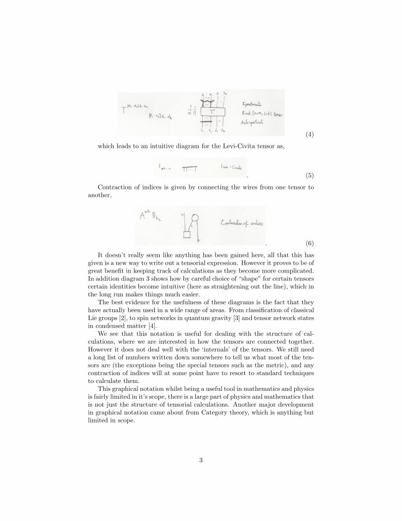
(4)

which leads to an intuitive diagram for the Levi-Civita tensor as,

. (5)

Contraction of indices is given by connecting the wires from one tensor toanother,

. (6)

It doesn’t really seem like anything has been gained here, all that this hasgiven is a new way to write out a tensorial expression. However it proves to be ofgreat benefit in keeping track of calculations as they become more complicated.In addition diagram 3 shows how by careful choice of “shape” for certain tensorscertain identities become intuitive (here as straightening out the line), which inthe long run makes things much easier.

The best evidence for the usefulness of these diagrams is the fact that theyhave actually been used in a wide range of areas. From classification of classicalLie groups [2], to spin networks in quantum gravity [3] and tensor network statesin condensed matter [4].

We see that this notation is useful for dealing with the structure of cal-culations, where we are interested in how the tensors are connected together.However it does not deal well with the ‘internals’ of the tensors. We still needa long list of numbers written down somewhere to tell us what most of the ten-sors are (the exceptions being the special tensors such as the metric), and anycontraction of indices will at some point have to resort to standard techniquesto calculate them.

This graphical notation whilst being a useful tool in mathematics and physicsis fairly limited in it’s scope, there is a large part of physics and mathematics thatis not just the structure of tensorial calculations. Another major developmentin graphical notation came about from Category theory, which is anything butlimited in scope.

3

1.2 Category theory

Category theory was originally developed by Saunders MacLane and SamuelEilenberg [5], in the context of topology but was quickly used to study abstractstructures in mathematics and later in computer science [6] and physics [7]. Theoverarching theme in category theory is to not worry about the the propertiesof the objects to be studied but to consider only how they interact and relateto each other [8].

A category C is defined [8] as a collection of ‘objects’, |C|, together with aset of ‘morphisms’, C(A,B), for each pair of objects, A,B ∈ |C|.

Along with a binary operation,

◦ : C(B,C)× C(A,B)→ C(A,C),

which is associative,(f ◦ g) ◦ h = f ◦ (g ◦ h),

and there exists an identity,

IA ∈ C(A,A) ∀ A ∈ |C|,

such that,f ◦ IA = f = IB ◦ f ∀ f ∈ C(A,B).

From this definition it is not at all clear what this would have to do withdiagrammatic notation at all, the first step in that direction is by introducingthe idea that the morphisms can be drawn as arrows going between the objects.

i.e. if f ∈ C(A,B) then this can be written as f : A→ B or even just Af- B.

The binary operation can then be seen just as connecting two of these arrows

end to end to create another arrow, e.g. Af- B

g- C = Ag◦f- C. And

the identity is an arrow from an object to itself AIA- A.

Larger networks of these arrows can be built up connecting many differentobjects together to create larger diagrams, a useful property of such a diagram iswhether it ‘commutes’ or not. This means that whichever route we take betweentwo objects in a given diagram will result in the same morphism. Many proofs incategory theory boil down to determining whether a given diagram commutes.

Despite diagrammatic notation appearing at this point it is not actuallythese diagrams that we are primarily interested in. The diagrams we are actuallyinterested in can be seen as an extension of this sort of reasoning to ‘monoidalcategories’, where ‘string diagrams’[9] can be used.

A strict monoidal category[10] M is a category equipped with an operator,

⊗ :M×M→M,

and a unit object 1.Such that (A⊗ B)⊗ C = A⊗ (B ⊗ C) and 1⊗ A = A = A⊗ 1. Note that

in the case where the monoidal category is not strict these equalities become‘natural isomorphisms’ subject to certain ‘coherence conditions’.

4

There is a more physical interpretation of monoidal categories in terms of‘process theories’[10] if we have a category where the objects are some physicalobjects and the morphisms are some physical process that we can do to trans-form one object into another. In such a category we can imagine that there aretwo types of composition that we would want. Firstly, we could do one physicalprocess first and then do another to the same object, providing that the objectsand transformations match up correctly. This corresponds to the ◦ compositionof morphisms in a category. The second type of composition corresponds todoing two processes at the same time to a pair of objects, that is the monoidaloperation ⊗.

From this viewpoint it is clear that these two products should interact in aparticular way, this is the ‘interchange law’. In words it says that (for suitableprocesses f, g, h, i on a suitable pair of objects) “doing (f and g) then (h and i)to a pair of objects” will be the same as “doing (f then h) and (g then i) to thesame pair of objects”. Or in the monoidal category language (f ⊗ g) ◦ (h⊗ i) =(f ◦h)⊗ (g ◦ i). This can be proved to be true from the definition of a monoidalcategory.

We now explain the diagrammatic notation for such a process theory, i.e.string diagrams [9]. Like with Penrose graphical notation certain non-obviousequations become utterly trivial when expressed in the new language which gives

some suggestion of it’s later use. A morphism Af- B is notated as,

. (7)

composition as,

. (8)

monoidal product as,

5

. (9)

and the interchange law becomes tautological,

. (10)

We can generalise this to include processes that take any number of objectsto any other number of objects, and so include boxes with arbitrary numbers ofinputs and outputs e.g.,

. (11)

Bob Coecke and Samson Abramsky [11] developed this notation for use inquantum mechanics in terms of a (dagger compact symmetric) monoidal cate-gory. This is based on the ideas described above but greatly extended, there isnot space in this review to go into all of the details but an illustrative exampleusing many of the important features will be shown in the next section.

A good review of the different diagrammatic notation used in category theoryis by P. Selinger [12]. It is also worth noting at this point that Penrose’s graphicalnotation can now also be thought of in this language as an example of a stringdiagram.

There are many examples of diagrammatic notations used now in physics,many of these can be thought of from a categorical perspective but many arenot (yet!). In the following sections I hope to introduce at least a few of thesebut obviously this cannot be an entirely comprehensive review.

6

2 Diagrams for calculations

In this section we try to motivate the development of these diagrammatic lan-guages from a pragmatic point of view, i.e. that they speed up ones ability to docalculations in physics. An example of this would be Feynman diagrams, theyprovide a way to perform complicated integrals using a perturbative method inwhich each term in the perturbation series is “easy” to calculate, in addition itprovides a physical intuition of what is happening in the diagrams i.e. a sumof all the possible ways in which particles can interact [13]. It is worth men-tioning however that recent developments (for example the amplituhedron [14]in N = 4 SYM) imply that Feynman diagrams may not be the optimal tool,and that perhaps this intuitive picture, in its simplicity, has hidden the realunderlying structure (perhaps there’s a lesson to be learnt here...).

We now consider two example calculations and show how diagrammaticmethods can provide a simpler way of performing calculations in quantum me-chanics. We begin with cluster state quantum computing [15] and then consideran example from condensed matter, the toric code [16]. We will compare howstandard Dirac notation performs in these two examples against modern dia-grammatic notations.

2.1 Cluster state quantum computing

Cluster state quantum computing [15], is a way of performing a quantum com-putation which has three stages. In the first a ‘cluster state’ is prepared. This isachieved by first initialising a number of qubits in the state |+〉 = (1/

√2)(|0〉+

|1〉 and then applying a number of CZ = |00〉〈00|+ |01〉〈01|+ |10〉〈10|− |11〉〈11|unitary operators to some pairs of these qubits. Any state formed in this wayis a cluster state, but we will use a particular example here, a ‘linear cluster offour qubits’. We will label these qubits by i ∈ 1, 2, 3, 4.

The second stage involves measuring qubits in the bases |±α〉 := (1/√

2)(|0〉±eiα|1〉), where a different value of the phase α is picked for each qubit. This“simulates” the unitary evolution process in standard quantum computing, thisis what our example calculation will show.

The final stage is to apply some Pauli corrections to counteract for gettingthe ‘wrong’ measurement outcomes, this can be combined into the final mea-surement step in the computational basis.

In this example we show a standard result, that is that given a linear clusterwhere the first qubit is prepared in state |ψ〉 it is possible by performing threemeasurements to project the fourth qubit into the state HU |ψ〉 where the threeangles correspond to the angles in an Euler decomposition of the unitary U .

Firstly using Dirac notation, we begin with the state,

|ψ1 +2 +3+4〉,

apply the CZ unitaries,

CZ12CZ23CZ34|ψ1 +2 +3+4〉,

7

and then measure the first three qubits, assuming we get the correct (i.e. +αnot −α) outcomes, then (up to normalisation) the state of qubit 4 at the endof this process will be,

|φ4〉 = 〈α1β2γ3|CZ12CZ23CZ34|ψ1 +2 +3+4〉.

We have suppressed identity unitaries in the above for simplicity but themeaning should be clear (for example CZ23 := 11 ⊗ CZ23 ⊗ 14). We define|ψ〉 := A|0〉+B|1〉.

Now for the long and tedious calculation,

|φ4〉 = 〈α1β2γ3|CZ12CZ23CZ34|ψ1 +2 +3+4〉 (12)

= 〈α1β2|CZ12|ψ1〉〈γ3|CZ23CZ34|+2 +3 +4〉 (13)

=1

2((〈0|+ e−iα〈1|)1(〈0|+ e−iβ |1〉)2CZ12(A|0〉+B|1〉)〈γ3|CZ23CZ34|+2 +3 +4〉 (14)

=1

2((A+Be−iα)〈02|+ e−iβ(A−Be−iα)〈12|)〈γ3|CZ23CZ34|+2 +3 +4〉 (15)

=1

2((A+Be−iα)〈02|+ e−iβ(A−Be−iα)〈12|)〈γ3|CZ23|+2〉CZ34|+3+4〉 (16)

=1

4((A+Be−iα)〈02|+ e−iβ(A−Be−iα)〈12|)(〈0|+ e−iγ〈1|)CZ23(|0〉+ |1〉)CZ34|+3+4〉 (17)

=1

4((A+Be−iα + e−iβ(A−Be−iα))〈03|+ e−iγ(A+Be−iα − e−iβ(A−Be−iα))〈13|)CZ34|+3+4〉 (18)

=1

8((A+Be−iα + e−iβ(A−Be−iα))〈03|+ e−iγ(A+Be−iα − e−iβ(A−Be−iα))〈13|)(|00〉+ |01〉+ |10〉 − |11〉)(19)

=1

4√

2((A+Be−iα + e−iβ(A−Be−iα))|+4〉+ e−iγ(A+Be−iα − e−iβ(A−Be−iα))〈−4|) (20)

H|φ4〉 =1

4√

2(A((1 + e−iβ)|04〉+ (1− e−iβ)e−iγ |14〉) +B((1− e−iβ)|04〉+ (1 + e−iβ)e−iγ |14〉))(21)

= U(A|0〉+B|1〉) (22)

(23)

|φ4〉 = HU |ψ〉

The above is an outline of the calculation, I got bored at the end and skippeda lot of it but the idea is there, its not difficult but not very fun either. The samecalculation could be done with matrices but that would be even more tediousand doesn’t highlight the physics of what is happening.

We next show how the calculation can be done using the notation of Co-ecke and Abramsky [17], we explicitly use this below and show what graphicalidentity is used at each step. Once one is relatively familiar with these the cal-culation can essentially be done without writing anything down apart from theinitial picture of the calculation.

8

Again we initialise the state as |ψ + ++〉, this is drawn as,

. (24)

apply the CZ operations, (there has actually been a graphical rule usedalready in this stage, the ‘spider rule’ which we will come back to later),

. (25)

measure the first three qubits,

. (26)

.This is the initial diagram that one would write down, it is just a graphical

description of the protocol being carried out.Next we start using some basic rewrite rules that let us put this diagram

into a simpler form, firstly the ‘spider rule’

. (27)

9

and then the ‘colour change rule’

. (28)

.At this point it is worth mentioning what these ‘spiders’ actually are, they

can be thought of either in terms of category theory, or more simply as a wayof keeping track of Dirac notation, as Penrose’s notation was for keeping trackof tensors. Taking this approach the spiders can be defined as,

. (29)

the relevant spiders in our diagram can now be seen to be,

10

. (30)

,

. (31)

and so we can see that we have Rz(γ)Rx(β)Rz(α) = U(α, β, γ) where thiscorresponds to an Euler decomposition of an arbitrary single qubit gate, U .Using these we can then finally write our diagram as,

. (32)

,and see that we have obtained the result we were looking for.

11

There are other methods that can be used to solve this problem, the onemost commonly used by people working on cluster states is ***check this*** acombination of cluster state diagrams (graph states), circuit diagrams and Diracnotation or alternatively using the stabiliser formalism provides a concise wayof performing these calculations. The brute force Dirac calculation is probablynot really used by anyone, particularly for more complicated situations.

Hardy [18] provides another graphical notation which looks fairly similar tocircuit diagrams or string diagrams. This notation is very useful for Hardy’sreformulation of quantum theory, in particular on providing an operationalistperspective on quantum theory, but they are difficult to use for practical calcu-lations.

2.2 Toric code

The Toric code can be thought of as the ground state of a Hamiltonian of asquare lattice. The Hamiltonian is,

H = −∑v

Av −∑p

Bp,

where v labels the vertices of the lattice and p the plaquette, (i.e. the squares).Av :=

∏i∈vXi and Bp :=

∏i∈p Zi, where i ∈ v means that the qubit i is

attached to vertex v and i ∈ p means that the qubit is part of the plaquette p.Often it is a hard problem to take a given Hamiltonian and determine it’s

ground state, in this case it is relatively simple as all of the terms in the Hamil-tonian commute. However for a large lattice it is difficult to write out the stateas it will contain a large number of terms and so there have been recent devel-opments in condensed matter to find efficient representations of states such asthese.

These efficient representations are called ‘tensor network states (TNS)’ wheredifferent shaped networks are used for different situations such as ‘matrix prod-uct states (MPS)’[19], ‘Projected Entangled Pairs (PEPS)’[19], ‘Multi-scale En-tanglement Renormalisation Ansatz (MERA)’[4].

A generic quantum state can be written as,

|ψ〉 =∑i1...in

ψi1...in |i1...in〉

, the coefficients ψi1...in can be thought of as a tensor. The basic idea of TNSs isthat this tensor which contains 2n complex coefficients, can for many interestingphysical situations, be more efficiently represented by considering a network ofsmaller tensors.

Graphically this network of tensors can be written using Penrose graphicalnotation. Where lines connecting tensors are just virtual summation indicesand unconnected lines correspond to the qubits. One could also interpret thesediagrams in terms of string diagrams, where the connecting lines would be some

12

quantum system being transferred between two quantum processes/interactions,unconnected lines would form the state once all interactions had occurred.

The Toric code as an efficient description as a PEPs tensor network[19],

(33)

.Here we see that there are two types of tensor in our network, these are,

(34)

the X tensors are entirely virtual as all of their indices are contracted, theT tensors have a disconnected index which corresponds to the physical state ofa qubit living at that point in the lattice. We use Greek indices for the virtualindices and roman letters for the state index.

Using this tensor network we can easily determine for any given configurationof qubits (i.e. state in the computational basis) what the amplitude for thatstate is.

By looking at this tensor network carefully one can see another interpretationof this toric code state, that is as a ‘string net condensate’[20].

First note that a valid description of a configuration for the qubits can begraphically written by colouring in the qubits in state |1〉 and doing nothing to

13

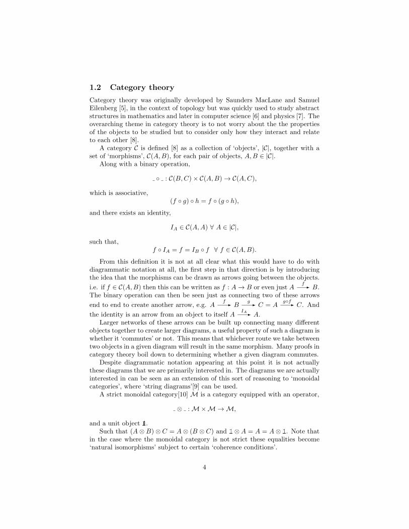
those in state |0〉. Equally valid would be to colour in the edge of the latticethat the |1〉 is on.

If we do this then we can note that the X tensors will only be non-zero whenthere are an even number of these coloured in edges going into them. e.g.

(35)

else they will give zero, e.g.,

(36)

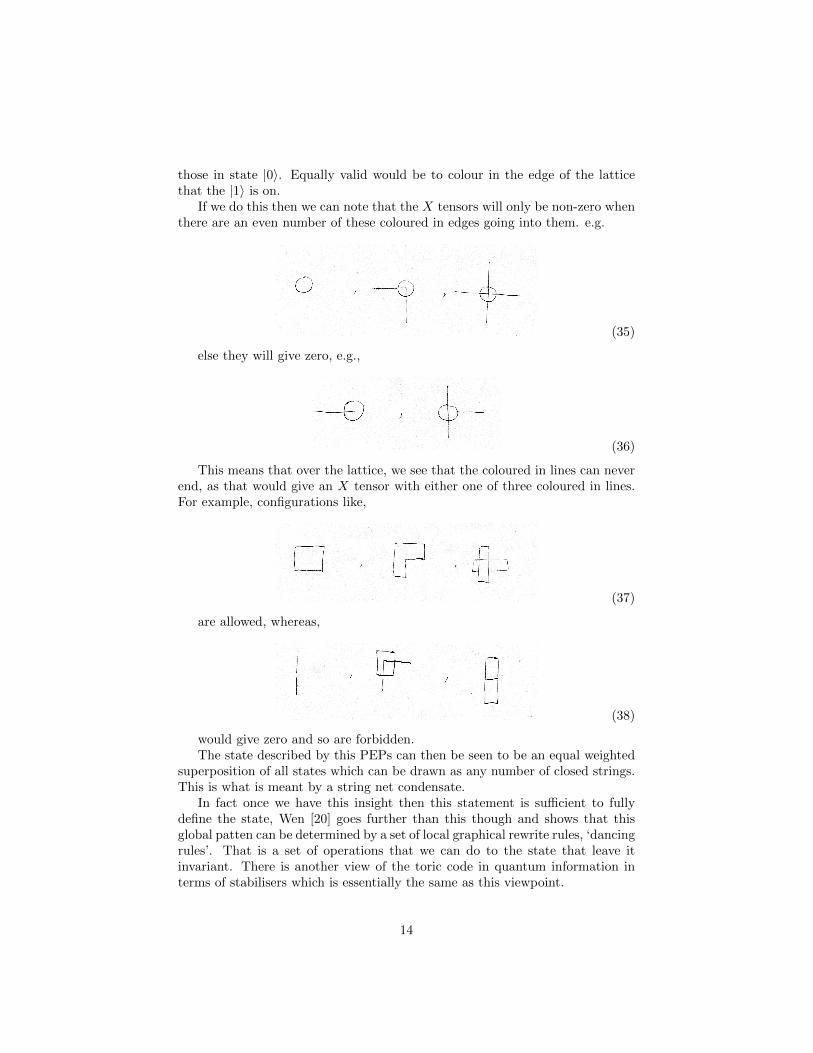
This means that over the lattice, we see that the coloured in lines can neverend, as that would give an X tensor with either one of three coloured in lines.For example, configurations like,

(37)

are allowed, whereas,

(38)

would give zero and so are forbidden.The state described by this PEPs can then be seen to be an equal weighted

superposition of all states which can be drawn as any number of closed strings.This is what is meant by a string net condensate.

In fact once we have this insight then this statement is sufficient to fullydefine the state, Wen [20] goes further than this though and shows that thisglobal patten can be determined by a set of local graphical rewrite rules, ‘dancingrules’. That is a set of operations that we can do to the state that leave itinvariant. There is another view of the toric code in quantum information interms of stabilisers which is essentially the same as this viewpoint.

14

The rules are,

(39)

this set of rules is sufficient to fully specify the state. This is a much moreconcise way of talking about the toric code then either the Dirac notation or theTNS description. Other sets of rules can be considered as well which would leadto different types of states in condensed matter such as, spin liquids, fractionalquantum hall states, superfluids and many others.

So we see here that not only does a diagrammatic viewpoint lead to a muchmore efficient description of the physics, it also gives physical insight that canlead to generalisations and new discoveries.

2.3 Where is this calculatory “power” come from?

It is interesting to try to consider why it is that diagrams seem to have thisability to both simplify calculations as well as to provide physical insight intothe world. One partial explanation may be that by using diagrams we areutilising a second dimension in our calculations, in standard mathematics areequations are strings of symbols in 1D, whereas when we move to using diagramswe utilise the full 2D plane of the paper we’re writing on. If we then considerwhat we try to do in 1D mathematics it appears to be a compression of this2D mathematics onto 1D. For example in process theories when we have bothparallel and sequential composition we need to introduce ◦ and ⊗ to take thisinto account and then impose some axioms about how they interact. From thisviewpoint the 2D mathematics is far more natural, and the compression to 1Dhides the true nature of what is going on.

Yet despite the naturality of these diagrams, in all of the examples we areusing above we are always at some level resorting to use of 1D mathematics. Interms of Penrose graphical notation it’s built on the foundations of tensors andlinear algebra, and the string diagrams are built on category theory, all of whichare defined in 1D notation. Even in Hardy’s notation which is built on the ideasof diagrams and composition, he provides a translation to 1D mathematics topersuade people of the rigour of his calculations.

Mathematics fundamentally can be viewed in terms of formal systems, anaxiomatic way to determine the ‘truth’ of a set of symbols [21]. There is no a

15

priori reason that this necessitates the symbols to be arranged in one dimen-sional strings. So we suggest that resorting to one dimensional mathematicsis not inevitable and should be something we should work towards avoiding asdiagrammatic reasoning appears to be a far more natural approach.

Another illustrative analogy that can be drawn is to computer science. Incomputer science everything at its most fundamental is based on long stringsof binary, but no programmer would ever try to write a large program usingthis language. Instead there are many layers of abstraction between the ma-chine code up to the programming language that is actually used. Similarly, wecan view matrix calculations in quantum mechanics as the equivalent of binaryand see first Dirac notation and then string diagrams built as ‘higher level’ lan-guages on top of this. This analogy may be particularly pertinent to quantumcomputing if large scale quantum computers are ever realised.

The diagrams discussed in this section are not universally useful or applica-ble. The ‘dancing rules’ of Wen do not appear to be relevant to all instanceswhere a TNS could be used. And cluster state diagrams and stabiliser formal-ism are not applicable to all quantum information protocols. Yet when they areuseful they seem to be the most concise and elegant way to perform calculations.We see that their appears to be some trade off between how widely applicablea language is vs. how powerful it is for a particular situation. Another exampleis Hardy’s duotensor notation [18], this is highly specialised for the particularreformulation of Hardy and is very powerful in that context, however in termsof general calculations in quantum mechanics it is much more cumbersome thanthe notation of Coecke and Abramsky.

3 Conclusion

3.1 Unification of the different notations

We have now seen various different examples of diagrammatic notation beingused in physics. Many of these could be interpreted as diagrams in a monoidalcategory. All of the string diagrams, Penrose graphical notation and tensornetworks [22] have a categorical interpretation. Feynman diagrams can also beinterpreted as a string diagram [7]. So it seems like category theory may providea rigorous underpinning for all of the diagrammatic notation used in physics,Baez and many others are working on turning anything that remotely looks likea network into diagrams in some category, from electric circuits [23] to Petrinets [24] to Bayesian networks[23].

One set of diagrams that we have talked about so far that hasn’t been tiedto category theory is the string nets of Xiao-Gang Wen , however it turns outthat the possible states described by dancing rules is classified by using tensorcategory theory [20] so it seems that category theory is just under the surfacehere as well. The other diagram currently not linked to category theory areHardy’s operator tensor diagrams, as far as I know this has not yet been donebut there is no obvious reason why they could not be interpreted as diagrams

16

in a monoidal category.It is not yet clear whether category theory will underly all diagrammatic

languages but it is clear that it is a powerful unifying tool in physics as it was inmathematics. It provides a broad framework to work upon which can describe awide range of physics, mathematics and computer science whilst once specialisedfor a particular task, e.g. the string diagrams of Coecke and Abramsky, alsobecomes a powerful tool for calculation. The hope is that the simplicity of thenotation and graphical manipulations will lead to not just easier pen and papercalculations but also the possibility of automated reasoning [25].

3.2 Hardy’s compositional principle

The line between diagrams used to describe a situation and a mathematicaldiagrammatic notation are often blurred. For example in the cluster state no-tation one could imagine that we had four qubits that were actually in a line,that then were passed through some entangling gates and then measured, thediagram could then correspond to just a picture of the experiment, where boxesrepresent the real physical processes and the lines real physical systems. Equallywell the diagrams can be viewed purely as mathematical notation, used to cal-culate the final state. Hardy [26] takes this idea as a primitive and suggeststhat there should be a ‘compositional principle’ that theories should aspire to,that is that the mathematical calculation performed should be composed in thesame way as the physical objects which the calculation is about.

From a category theory point of view this amounts to saying that if we canrepresent the composition of some object by a diagram in some ‘real world’category, then their should exist some functor from that category to a concretecategory in which the properties of that object can be calculated.

3.3 Beyond 2D

Throughout this review we have highlighted the increased descriptive power andease of calculation that arises from moving from 1D to 2D mathematics, it isnatural to consider what happens if we move beyond 2D. Within the context ofmonoidal categories it can be said that if we introduce a ‘braiding’ operator, i.e.one that interchanges lines, then this gives a 3D diagram as now we draw objectscrossing which must take place off the plane. Symmetric monoidal categoriesare those in which if we apply this braiding twice we end up with the same, i.e.we can unknot any lines, this can be viewed as drawing a 4D diagram as in 4Dall knots can be trivially untied. So in some sense we can already depict higherdimensions within the same framework.

This is not the whole story thought, we are still limiting ourselves to 1Dstrings living in potentially higher dimensional spaces. We can also considerwhat occurs if we allow for (hyper) surfaces, these sorts of objects arise nat-urally when one considers n-categories, for example in a string diagram for a2-Category the diagrammatic elements are given by, points, lines and surfaces,there is recent work in using bicategories for quantum protocols [27].

17

3.4 Summary

To briefly summarise, in this overview we began by discussing some of the his-tory of diagrammatic notations in physics, the original example being Penrose’sgraphical notation for tensors. We then briefly discussed how category theoryplays a role in giving a formal mathematical basis for many of the diagramsthat we use today in physics despite its routes lying in highly abstract mathe-matics. We then gave a couple of examples in which diagrams can be used tomake calculations and descriptions of states far simpler, cluster state quantumcomputing and the toric code. Finally looking at what it is that gives these di-agrammatic notations their power and considering what the natural extensionsto these could be in terms of higher category theory.

I have mainly highlighted the use of these diagrammatic notations for theirability to make calculations easier and more natural, my main hope howeveris that by viewing quantum theory through this lens we will be able to gain adeeper understanding of it.

References

[1] Roger Penrose. Applications of negative dimensional tensors. Combinato-rial mathematics and its applications, 221244, 1971.

[2] Predrag Cvitanovic. Group Theory: Birdtracks, Lie’s, and ExceptionalGroups. Princeton University Press, 2008.

[3] C Rovelli and L Smolin. Spin networks and quantum gravity. Physicalreview D: Particles and fields, 52(10):5743–5759, November 1995.

[4] Guifre Vidal. Entanglement Renormalization: an introduction. arXivpreprint arXiv:0912.1651, page 24, December 2009.

[5] Samuel Eilenberg and Saunders MacLane. General theory of natural equiva-lences. Transactions of the American Mathematical Society, 58(2):231–294,1945.

[6] Joseph A. Goguen. A categorical manifesto. In Mathematical Structures inComputer Science, pages 49–67, 1991.

[7] John C Baez and Aaron Lauda. A Prehistory of n -Categorical Physics.pages 1–129, 2009.

[8] Samson Abramsky and Nikos Tzevelekos. Introduction to categories andcategorical logic. In New structures for physics, pages 3–94. Springer, 2011.

[9] Andre Joyal and Ross Street. The geometry of tensor calculus ii. Draftavailable at http://www. math. mq. edu. au/˜ street/GTCII. pdf, 585, 1991.

[10] Bob Coecke and Eric Oliver Paquette. Categories for the practising physi-cist. In New structures for physics, pages 173–286. Springer, 2011.

18

[11] Samson Abramsky and Bob Coecke. A categorical semantics of quantumprotocols.

[12] Peter Selinger. A survey of graphical languages for monoidal categories.In New Structures for Physics, pages 289–355. Springer Berlin/Heidelberg,2011.

[13] Michael E. Peskin and Daniel V. Schroeder. An Introduction to QuantumField Theory. Perseus Books, Cambridge, Massachusetts, 1995.

[14] Nima Arkani-Hamed and Jaroslav Trnka. The Amplituhedron. page 36,December 2013.

[15] Michael A Nielsen. Cluster-state quantum computation. XX(X):15, April2005.

[16] AY Kitaev. Fault-tolerant quantum computation by anyons. Annals ofPhysics, page 27, July 2003.

[17] Bob Coecke. Quantum Picturalism. Contemporary physics, page 31, August2009.

[18] Lucien Hardy. The Operator Tensor Formulation of Quantum Theory.page 37, January 2012.

[19] Roman Orus. A Practical Introduction to Tensor Networks: Matrix Prod-uct States and Projected Entangled Pair States. page 51, June 2013.

[20] Xiao-gang Wen. Topological order: from long-range entangled quantummatter to a unified origin of light and electrons. pages 0–42.

[21] H.B. Curry. Outlines of a Formalist Philosophy of Mathematics. Studiesin logic and the foundations of mathematics. Elsevier Science, 1951.

[22] JD Biamonte, SR Clark, and Dieter Jaksch. Categorical tensor networkstates. AIP Advances, page 39, December 2011.

[23] Brendan Fong. Causal Theories: A Categorical Perspective on BayesianNetworks. page 72, January 2013.

[24] John C Baez and Jacob D Biamonte. A Course on Quantum Techniquesfor Stochastic Mechanics.

[25] Lucas Dixon and Ross Duncan. Extending graphical representations forcompact closed categories with applications to symbolic quantum com-putation. In Serge Autexier, John Campbell, Julio Rubio, Volker Sorge,Masakazu Suzuki, and Freek Wiedijk, editors, Intelligent Computer Math-ematics, 9th International Conference, AISC 2008, 15th Symposium, Cal-culemus 2008, 7th International Conference, MKM 2008, Birmingham,UK, July 28 - August 1, 2008. Proceedings, volume 5144 of Lecture Notesin Computer Science, pages 77–92. Springer, 2008.

19

[26] Lucien Hardy. On the theory of composition in physics. arXiv preprintarXiv:1303.1537, March 2013.

[27] Mike Stay and Jamie Vicary. Bicategorical Semantics for NondeterministicComputation. page 21, January 2013.

20