an overview of exact and approximate algorithms

European Journal of Operational Research 59 (1992) 231-247 231 North-Holland

Invited Review

The Traveling Salesman Problem: An overview of exact and approximate algorithms

Gilbert Laporte Centre de recherche sur les transports, Universit~ de Montr&l, C.P. 6128, Station A, Montreal, Canada H3C M7

Received May 1991; received July 1991

Abstract: In this paper, some of the main known algorithms for the traveling salesman problem are surveyed. The paper is organized as follows: 1) definition; 2) applications; 3) complexity analysis; 4) exact algorithms; 5) heuristic algorithms; 6) conclusion.

Keywords: Traveling salesman problem; survey

Introduction

The Traveling Salesman Problem (TSP) is one of the most widely studied combinatorial optimization problems. Its s tatement is deceptively simple, and yet it remains one of the most chal- lenging problems in Operat ional Research. Hun- dreds of articles have been written on the TSP. The book edited by Lawler et al. (1985) provides an insightful and comprehensive survey of all major research results until that date. The pur- pose of this survey paper is less ambitious. Our main objective is to present an integrated overview of some of the best exact and approximate algorithms so far developed for the TSP, at a level appropriate for a first graduate course in combinatorial optimization.

C : (Cij) be a distance (or cost) matrix associated with A. The TSP consists of determining a minimum distance circuit passing through each vertex once and only once. Such a circuit is known as a tour or Hamiltonian circuit (or cycle). In several applications, C can also be interpreted as a cost or travel time matrix. It will be useful to distin- guish between the cases where C (or the problem) is symmetrical, i.e. when c u = cyi for all i,j ~ V, and the case where it is asymmetrical. Also, C is said to satisfy the triangle inequality if and only if Cij q- Cjk ~ Cik for all i,j,k ~ V. This occurs in Euclidean problems, i.e. when V is a set of points in ~2 and c~ is the straight-line distance between i and j.

2. Applications

I. Definition

Let G = (V, A) be a graph where V is a set of n vertices. A is a set of arcs or edges, and let

The most common practical interpretation of the TSP is that of a salesman seeking the shortest tour through n clients or cities. This basic problem underlies several vehicle routing applications,

0377-2217/92/$05.00 © 1992 - Elsevier Science Publishers B.V. All rights reserved

232 G. Laporte / The travefing salesman problem: Overview of algorithms

but in this case a number of side constraints usually come into play (see Laporte, 1992). Sev- eral interesting permutat ion problems not directly associated with routing can also be described as TSPs. Here are some selected exam- pies.

1. C o m p u t e r wiring (Lenstra and Rinnooy Kan, 1975). Some computer systems can be described as modules with pins attached to them. It is often desired to link these pins by means of wires, so that exactly two wires are attached to each pin and total wire length is minimized.

2. Wallpaper cut t ing (Garfinkel, 1977). Here, n sheets must be cut from a roll of wallpaper on which a pat tern of length 1 is repeated. For sheet i, denote by a i and b i the starting and ending points on the pattern, where 0 ~< a i ~< 1 and 0 ~< b i

1. Then cutting sheet j immediately after sheet i results in a waste of

aj - b i if b i <~ aj ,

cij = ~ 1 + a t - b i if b i > a j . ( 1 )

The objective is to order the n sheets so as to minimize total waste. In order to define the problem as a TSP, consider a dummy sheet n + 1 with Ci ,n+ 1 = 0 and cn+ 1,~' = 0 for all i , j = 1 . . . . . n. A l - ternatively, define bn+ 1 as the end of the roll position at the start of cutting and assume that after the last sheet, a final cut must be made to restore the row to its original position. Then an+ 1 = b , + l , and cij can be defined as in (1) for all i , j = 1 . . . . . n + 1.

3. Hole punch ing (Reinelt, 1989). In several manufacturing contexts, it is necessary to punch holes on boards or metallic sheets. The problem consists of determining a minimum-time punch- ing sequence. Such a problem occurs frequently in metallic sheet manufacturing and in the construction of circuit boards. These problems are often of large scale and must be solved in real- time.

4. Job sequencing. Suppose n jobs must be performed sequentially on a single machine and that cij is the change-over time if job j is executed immediately after job i. Then again, by introducting a dummy job, this problem can be formulated as a TSP.

5. Dar tboard design (Eiselt and Laporte, 1991). Dartboards are circular targets with concentric circles, and 20 sectors identified by the numbers 1

to 20. Players throw darts at target points on the board. In the most common version of the game, the objective is to reduce an initial value of 301 to zero by substracting scores. The game rewards accuracy in the throw and it is often more important to hit one's target that to merely register a large score. A natural objective for designing a dartboard is therefore to position the 20 numbers around the board so as to maximize players' risk. For fairly accurate players, it is reasonable to assume that the sector that is hit is always the targeted sector or its neighbour. Let ~ - = (rr(1) . . . . . ¢r(20)) be any permutat ion of the numbers 1 . . . . . 20. In what follows, ~-(k) must be interpreted as ~-(k mod 20) whenever k < 1 or k > 20. Consider a player aiming at ~-(k) and hitting 7r(k + 1) with probability p, and 7r(k) with probability 1 - 2p. For this player, the expected deviation from the aimed score is equal to p[~r(k - 1) - 7r(k)] +p[Tr(k + 1) - or(k)]. A possible objective is to maximize the expected sum of square deviations, i.e. Y'.2°a{p[~-(k - 1) - 7r(k)] 2 + p [ T r ( k + 1)-Tr(k)]2}. Since p is a constant, this is equivalent to solving a TSP with cii = (i - j)2.

6. Crys ta l lography (Bland and Shallcross, 1989). In crystallography, some experiments con- sist of taking a large number of X-ray intensity measurements on crystals by means of a detector. Each measurement requires that a sample of the crystal be mounted on an apparatus and that the detector be positioned appropriately. The order in which the various measurements on a given crystal are made can be seen as the solution of a TSP. In practice, these problems are of large scale and obtaining good TSP solutions can reduce considerably the time needed to carry out all measurements.

3. Complexity

In order to study the complexity of the traveling salesman problem first consider the following well-known decision problem:

H A M I L T O N I A N C I R C U I T (HC) Instance: A graph G = (V, A). Question: Does G contain a Hamiltonian circuit?

It is well known that HC is NP-complete (Garey and Johnson, 1979, p. 47). We show that TSP is

G. Laporte / The traveling salesman problem: Overview of algorithms 233

NP-hard by using the following transformation. Given any instance of HC relative to a graph G h = (V h, A h) with vertex set V h = {1 . . . . . n} and arc set A h = {(i, j)}, define a TSP instance having V = V h, A = { ( i , j ) : i , j = l , . . . , n , i4=j} and cii = 1 if (i, j ) ~ A h and cir = m, otherwise. Then G contains a Hamiltonian circuit if and only if the optimal value of the TSP instance is equal to n.

A number of special cases of TSP are, however, solvable in polynomial time (see, for example, Gilmore, Lawler and Shmoys, 1985). Exam- ples of such problems include:

1. TSPs where C = (cij) is an upper triangular matrix, i.e. cij = 0 for all i > j ;

2. The wallpaper cutting problem described in Section 2;

3. A class of job sequencing problems defined by Gilmore and Gomory (1964). In this problem, there are n - 1 jobs to be processed sequentially in a kiln. Job i requires a starting tempera ture of a i and must be finished at tempera ture b i. Fur- ther assume that the initial kiln tempera ture is a n and that the final tempera ture must be b n. Then the problem can be formulated as a TSP with

c i j

ifa <.bi - ¢ 1 i

where f and g are cost density functions and f ( x ) + g (x ) > 0 for all x since otherwise, it would be profitable to keep changing the kiln tempera- ture.

4. E x a c t a l g o r i t h m s

A large number of exact algorithms have been proposed for the TSP. These can be best under- stood and explained in the context of integer linear programming (ILP). We examine in this section a number of ILP formulations and of algorithms derived from these formulations.

4.1. Integer linear programming formulations

One of the earliest formulations is due to Dantzig, Fulkerson and Johnson (DFJ) (1954). It associates one binary variable x/j to every arc

(i, j), equal to 1 if and only if (i, j ) is used in the optimal solution, i =~j. The DFJ formulation is (DFJ)

Minimize ~ cijxij ( 2 ) i4=j

subject to ~_~ xij = 1, i = 1 . . . . , n, (3) j=l

n

~ X i j = 1, j = 1 . . . . . n, (4) i - 1

£ Xi j< I S I - 1 , i , j~s

S c V , 2 ~ IS] ~ < n - 2 , (5)

xij ~ {0, 1},

i, j = 1 . . . . . n, i :~j. (6)

In this formulation, the objective function clearly describes the cost of the optimal tour. Constraints (3) and (4) are degree constraints: they specify that every vertex is entered exactly once (3) and left exactly once (4). Constraints (5) are subtour elimination constraints: they prohibit the formation of subtours, i.e. tours on subsets of less than n vertices. If there was such a subtour on a subset S of vertices, this subtour would contain I S I arcs and as many vertices. Constraint (5) would then be violated for this subset since its left-hand side would be equal to I S[ and its right-hand side equal to IS I - 1. Because of degree constraints, subtours over one vertex (and hence, over n - 1 vertices) cannot occur. There- fore it is valid to define constraints (5) for 2 ~< I S I ~< n - 2 only. Finally, constraints (6) impose binary conditions on the variables.

An alternative equivalent form of constraints (5) is

£ £ X i j > / 1 S c V , 2 < ISl < n - 2 (5 ' ) i~S j~3

where S = V \ S . Constraints (5 ') can be derived from (5) by noting that every vertex i of S is the origin of one arc to another vertex of S or to a vertex of S. Since there are [SI vertices, I S[ = ~i,j~sXij a t- ~i~S~j~_~Xij, and the equivalence of (5) and (5') follows trivially. The geometric inter- pretat ion of connectivity constraints (5 ') is that in every TSP solution, there must be at least one arc pointing from S to its complement, in other words, S cannot be disconnected.

234 G. Laporte / The traveling salesman problem: Overview of algorithms

This formulation contains n ( n - 1) binary variables, 2n degree constraints and 2 n - 2n - 2 subtour elimination constraints. Even for moderate values of n, it is unrealistic to solve DFJ directly by means of an ILP code. The model is usually relaxed, and solved by means of specialized algorithms.

Miller, Tucker and Zemlin (MTZ) (1960) have proposed an alternative formulation that reduces the number of subtour elimination constraints at the expense of extra variables u i (i = 2 . . . . . n). The MTZ subtour elimination constraints can be expressed as

U i - - Uj + ( n - 1 ) x i j <~ n - 2

i , j = 2 . . . . , n , i 4: j , (7)

l < ~ u i < ~ n - 1 i = 2 . . . . . n. (8)

Constraints (7) ensure that the solution contains no subtour on a set of vertices S c_ V\{1} and hence, no subtour involving less than n vertices. Constraints (8) ensure that the u i variables are uniquely defined for any feasible tour. In order to see how constraints (7) operate, suppose there was a subtour (il, i 2 . . . . . i k , il) with k < n. Writing constraints (7) for every arc of that subtour gives

U i l - - U i 2 + ( n - 1) ~<n - 2 ,

l,li2--Ui3+ ( n -- 1) -<<n - 2,

u i k - ui, + ( n - 1) ~ n - 2.

Summing up these constraints yields k ( n - 1) ~< k ( n - 2), a contradiction.

It has been observed recently (Desrochers and Laporte, 1991) that constraints (7) can be strengthened by introducing an extra term in their left-hand side to yield

U i - - Uj @ ( n - 1)Xi j + ( n - 3)Xji <~ n -- 2

i , j = Z , . . . , n , i ~ j . (9)

The validity of constraints (9) can be estab- lished as follows. Rewrite constraints (7) as

u i - u j + ( n - 1)Xi j + oljiXji ~ n - 2 (10)

where currently o Q i = O. We seek the largest possible value of aji so that (10) remains a valid inequality. In the optimal solution, xji can take only two values:

- if xji = 0, then (10) is satisfied for any aji;

- i f x j i = l , t h e n x i j = 0 ( f o r n > 2 ) a n d u j + l = u i, so that aji <~ n - 3.

In spite of its relative compactness, the MTZ formulation is weaker than the DFJ formulation in the following sense. D en o t e by z '(DFJ)[ z ' (MTZ)] the optimal value of the linear relaxation of DFJ [MTZ], i.e. the relaxation obtained by dropping integrality conditions. Then z ' (MTZ) ~< z ' (DFJ) (Wong , 1980). This result has not been proved for the modified MTZ formulation using constraints (9), but it is known that there exist cases where it produces a weaker linear relaxation than DFJ (Desrochers and La- porte, 1991).

Finally, a number of alternative formulations have been proposed and compared, but none of these seems to have a stronger linear relaxation than DFJ (Langevin, Soumis and Desrosiers, 1990).

4.2. The ass ignment lower bound and related

branch-and-bound algori thms

Branch-and-bound (BB) algorithms are commonly used for the solution of TSPs. In the context of mathematical programming, they can best be viewed as initially relaxing some of the problem constraints, and then regaining feasibility through an enumerative process. The quality of a BB algorithm is directly related to the quality of the bound provided by the relaxation.

For the TSP, an initial lower bound can be obtained from the DFJ formulation by relaxing constraints (5). The resulting problem is an assignment problem (AP) which can be solved in O ( n 3) time (see Carpaneto, Martello and Toth, 1988). Thus, a valid lower bound on the value of the optimal TSP solution is the AP bound defined by (2)-(4) and the nonnegativity require- ments on the variables.

Several authors have proposed BB algorithms for the TSP, based on the AP relaxation. These include Eastman (1958), Little et al. (1963), Shapiro (1966), Murty (1968), Bellmore and Mal- one (1971), Garfinkel (1973), Smith, Srinivasan and Thompson (1977), Carpaneto and Toth (1980), Balas and Christofides (1981) and Miller and Pekny (1991). We briefly describe the last three algorithms which are probably the best available.

G. Laporte / The traveling salesman problem." Overview of algorithms 235

In the Carpaneto and Toth algorithm, the problem solved at a generic node of the search tree is a modified assignment problem (i.e. x , is fixed at 0 for all i) in which s o m e x i j variables are fixed at 0 or at 1. If the AP solution consists of a unique tour over all vertices, it is then feasible for the TSP. Otherwise, it consists of a number of subtours. One of these subtours is selected and broken by creating subproblems in which all arcs of the subtour are in turn prohib- ited. We will use the following notation:

z*: the cost of the best TSP solution so far identified;

zh: the value of the objeiztive function of the modified AP at node h of the search tree;

Zh: a lower bound on Zh; Ih: the set of included arcs (x~j variables fixed

at 1) at node h of the search tree; Eh: the set of excluded arcs (xij variables fixed

at O) at node h of the search tree.

Step 1. (Initialization.) Obtain a first value for z* by means of a suitdble heuristic. Create node 1 of the search tree: set I 1 := E 1 := ~, and obtain z~ by solving the associated modified AP. If z~ >/ z*, stop: the heuristic solution is optimal. If the solution contains no illegal subtours, it consti- tutes the optimal tour: stop. Otherwise, insert node 1 in a queue.

Step 2. (Node selection.) If the queue is empty, stop. Otherwise, select the next node (node h) from the queue: here we use a breadth first rule, i.e. branching is always done on the pendant node having the lowest z h.

Step 3. (Subproblem partitioning.) The solution obtained at node h is illegal and must be elimi- nated by partitioning the current subproblem into descendant subproblems hr characterized by sets Ihr and Eh; In order to create these subproblems, consider a subtour having the least number s of arcs not belonging to I h. Let these arcs be (i 1, j~) . . . . . (i,, j~), in the order in which they appear in the subtours. Then create s subproblems with

I 1 k, r = l ,

Ih = l l h u { ( i , , , j ~ ) : u = l . . . . . r - - i } ,

r = 2 , . . . , s ,

Eh = E h U { ( i r , j r ) } , r = l . . . . . s.

Execute Step 4-6 for r = 1, . . . , s. Step 4. (Bounding.) Compute a lower bound

Zhr on Zhr by row and column reduction of the cost matrix. If Zhr < Z *, proceed to Step 5. Other- wise, consider the next r and repeat Step 4.

Step 5. (Subproblem solution.) Solve the subproblem associated with node h r (a modified AP restricted by Ih, and Ehr). If Zh~>Z*, consider the next r and proceed to Step 4.

Step 6. (Feasibility check). Check whether the current solution contains subtours. If it does, insert node h r in the queue. Otherwise, set z* := Zhr and store the tour, if z* = z h, go to Step 2.

Using their algorithm, Carpaneto and Toth have consistently solved randomly generated 240-vertex TSPs in less than one minute on a CDC 6600. The main limitation of this algorithm appears to be computed memory rather than CPU time.

The Balas and Christofides algorithm uses a s t ronger relaxation than the AP relaxation. Its description and the computational effort required for the lower-bound computat ions are much more involved, but the resulting search trees are smaller and the procedure is overall more powerful. Due to its complexity, it will only be sketched here. Interested readers are referred to the Balas and Christofides (1981) paper. In addition to constraints (3), (4) and (6), subtour elimination constraints (5), connectivity constraints (5 ') and some positive linear combinations of these are considered, and introduced into the objective function in a Lagrangean fashion. Let T be the set of all such constraints and t a given constraint. Their generic expression can be written as

y ' , a i j x i j ~ ao , t ~ T.

i , j~ V

The Lagrangean objective is then

A ) : m i n ( E c i j x i j - E L( A, x i , j ~ V t ~ T

~ i , j~ V

where A = (A 1 . . . . . A r ) is the vector of Lagrange multipliers, and x is any modified AP solution. The strongest relaxation is given by maxa~ 0 {L(A)}. As the number of components of A is


exponential, the required maximum is not deter- mined by Lagrangean relaxation. Instead, a lower bound on its value is obtained by restricting A to lie in the set {A > 0: Zlu,v ~ ~n, such that u~ + v/ +S, t~rAt a~j=cij if (i, j ) belongs to the AP solution; u~ + v/+ Et~rAt a~j > c~j, otherwise}. Balas and Christofides propose an approximation procedure for computing A. At a given node of the search tree, the procedure solves an AP with dual values given by u and v. It then computes A. A lower bound on the value of the TSP tour associated to that node of the search tree is given by

Eui + E vj+ EAt a°. (12) i ~ V j ~ V t ~ T

The authors then show how (12) can be computed for three particular classes of constraints (11). Using this procedure, Balas and Christofides report optimal solutions to randomly generated 325-vertex problems in less than one minute on a CDC 7600.

More recently, Miller and Pekny have proposed a new powerful BB algorithm based on the AP relaxation. Consider the dual AP: (DAP)

n n

Maximize ~_, u s + ~., vj (13) i=1 j = l

subject to eij - u i - vj >~ O

i , j = l , . . . , n , i ~ j . (14)

Denote by z*(TSP) the optimal TSP solution value, by z*(AP) the optimal value of the AP linear relaxation, and by z*(DAP) the optimal value of the dual AP linear relaxation. Clearly z*(AP) = z*(DAP). Moreover, note that z * ( A P ) + (c~j- u i - v j ) is a lower bound on the cost of an AP solution that includes arc (i, j). Miller and Pekny make use of this in an algorithm that initially removes from consideration all x~j variables whose cost c~j exceeds a threshold value A. Consider a modified problem TSP' with associated linear assignment relaxation AP ' and its dual DAP' , obtained by redefining the costs ci~ as follows:

, [c~j i f c , y < A , Cij = (15)

otherwise.

The authors prove the following proposition which they use as a basis for their algorithm: an optimal solution for TSP' is optimal for TSP if

z * ( T S P ' ) - z * ( A P ) ~<A + 1 - u ; - V ' ~ x (16)

and

! r a + 1 - u i - Uma x ~ 0 (17)

for i = 1 . . . . ,n , where u' and v' are optimal solutions to DAP' , and V'ax is the maximum element of v'. The quantity A + 1 - u~ - Vma x un- derestimates the smallest reduced cost of any discarded variable. The algorithm is then: Step 1 (Initialization). Choose A. Step 2 (TSP' solution). Construct (ci~) and solve

TSP' . Step 3 (Termination check). If (16) and (17) hold,

then z * ( T S P ' ) = z * ( T S P ) : stop. Other- wise, double A and go to Step 2.

The authors report that if A is suitably chosen in Step 1 (e.g., the largest arc cost in a heuristic solution), there is rarely any need to perform a second iteration. To solve TSP' , the authors have developed a BB algorithm based on the AP relaxation. They have applied this procedure to randomly generated problems. Instances involving up to 5000 vertices were solved within 40 seconds on a Sun 4 /330 computer. The largest problem reported solved by this approach contains 500000 vertices and required 12623 seconds of computing time on a Cray 2 supercomputer.

Finally, it is worth mentioning that in a different paper, Miller and Pekny (1989) describe a parallel branch-and-bound algorithm based on the AP relaxation. These authors report that randomly generated asymmetrical TSPs involving up to 3000 vertices have been solved to optimality using this approach.

4.3. The shortest spanning arborescence bound and a related algorithm

In a directed graph G = (F, A), an r-arborescence is a partial graph in which the in-degree of each vertex is exactly 1 and each vertex can be reached from the root vertex r. The shortest

G. Laporte / The traveling salesman problem. Overview of algorithms 237

spanning r-arborescence problem (r-SAP) can be formulated as

cijxij (18) i~j

subject to ~ xij = 1, j = 1 . . . . . n, (19) i = 1 i~j

E ~-,xij>>-l, S c V ; r ~ S , (20) i~S j ~ ,

x i j > ~ O , i , j = l . . . . . n , i - ~ j . (21)

The problem of determining a minimum-cost r-arborescence on G can be decomposed into two independent subproblems: determining a minimum-cost arborescence rooted at vertex r, and finding the minimum-cost arc entering vertex r. The first problem is easily solved in O(n 2) time (Tarjan, 1977). This relaxation can be used in conjunction with Lagrangian relaxation. How- ever, on asymmetric problems, the AP relaxation would appear empirically superior to the r- arborescence relaxation (Balas and Toth, 1977).

An early reference to this lower bound is made by Held and Karp (1970). More recently, Fis- chetti and Toth (1991) have used it within a so-called 'additive bounding procedure ' that com- bines five different bounds:

- the AP bound, - the shortest spanning 1-arborescence bound, - t h e shortest spanning 1-antiarborescence

bound 1 - SAAP; ( r -SAAP is defined in a manner similar to r-SAP but now it is required that vertex r should be reached from every remaining vertex),

- for r = 1 . . . . . n, a bound r-SADP obtained from r-SAP by adding the constraint

xrj = 1, (22) j~r

- for r = 1 , . . . , n, a bound r -SAADP obtained from r-SAAP by adding the constraint

E Xir = 1 . (23) i¢r

The lower-bounding procedure described by Fischetti and Toth was embedded within the Carpaneto and Toth (1980) branch-and-bound algorithm on a variety of randomly generated problems and on some problems described in the literature. The success of the algorithm depends

(r-SAP)

Minimize

on the type of problem considered. For the easi- est problem type, the authors report having solved 2000-vertex problems in an average time of 8329 seconds on an HP 9000/840 computer.

4.4. The shortest spanning tree bound and related algorithms

The AP-based algorithms described in the previous section are valid whether C is asymmetrical or symmetrical. However, in the latter case, the AP solutions will in general contain several subtours containing only two vertices, resulting in excessive computing times for their elimination. Symmetrical problems are bet ter handled by specialized algorithms that exploit their structure. We now describe an ILP formulation for symmetrical TSPs.

Consider a TSP defined on G = (V, E) where E is an edge set. Let xij be a binary variable equal to 1 if and only if edge (i, j ) is used in the optimal Solution. These variables are only defined for i < j. The formulation is then (SYM)

Minimize ~ CijXij i<j

subject to ~ xik + ~ xkj = 2, (24) i<k j>k

k = 1 . . . . . n, (25)

E Xij• I S I - 1 , i jEs (26)

S c V , 3 ~ [ S I ~ < n - 3 ,

xij ~ {0, 1}, (27)

i , j = l . . . . . n, i < j .

In this formulation, constraints (25) specify that every vertex has a degree of 2. Constraints (26) are subtour elimination constraints. They need not be defined for I SI = 2 and n - 2 since constraints (25) and (27) combined prevent the formation of subtours involving 2 (and thus n - 2) vertices. Constraints (27) impose binary conditions on the variables.

As for (DFJ), connectivity constraints equivalent to (26) can be derived. These can be written a s

~_~ xij>~2 , S c V , 3~< ISI ~ < n - 3 . i~S,j~S

or j~S,i~'S

(26 ' )


In order to show the equivalence of (26) and (26'), consider D(S) = )'~k~S(Ei<kXik + ~'j>k Xk), the sum of degrees of vertices of S. Every edge (i, j) for which i,j ~ S makes a contribution of 2 to D(S), whereas edges (i, j) with i ~ S, j ~ S or j ~ S, i ~ S contribute by only one unit. Hence,

o( s) = 2 E x,j + E x j, i , jeS iES,j~'S

orjeS,i~S

and the equivalence follows. A useful relaxation can be extracted from SYM

by exploiting the following consideration. In any feasible solution, the degree of vertex 1 must be equal to 2, while the remaining vertices must all be connected. A valid lower bound on the optimal TSP solution value is therefore the length of the shortest 1-spanning tree (1-SST), i.e. the shortest tree having vertex set V\{1}, together with two distinct edges at vertex 1. Formally, determining a least cost 1-SST is achieved by solving (1-SST)

Minimize ~ cijxij (28) i<j

subject to ~ xiy = n, (29) i<j

~ Xlj = 2, (30) j=2

E Xij~ 1, i~S,j~S\{1}

or j~S,i~S\{1}

S c V \ { 1 } , 1< ISl < n - l ,

(31) Xij ~ {0, 1}. (32)

redundant) to impose (27) for these values of IsI.

Christofides (1970) and Held and Karp (1971) were among the first to propose a TSP algorithm based on this relaxation. Improvements and re- finements were later suggested by Helbig Hansen and Krarup (1974), Smith and Thompson (1977), Volgenant and Jonker (1982), Gavish and Srikanth (1986), and Carpaneto, Fischetti and Toth (1989). In the original Held and Karp algorithm, the 1-SST bound is reinforced by introducing constraints (25) in the objective function to yield the Lagrangean

L(A) = min x

E CijXij i <j

k~V "i<k j>k

= m i n { Y'. E(cij--}-Ai+Aj)xij) x i~Vj>i

-- 2 )-'~ Ai, i ~v

where x is a feasible 1-SST solution. By performing dual ascents, Held and Karp obtain a lower bound on the strongest Lagrangean relaxation max~{L(a)}. This bounding process is embedded in a branch-and-bound scheme in the following manner. First define

z*: the cost of the best TSP solution so far identified;

Zh: the best lower bound on max~{L(h)} derived at node h of the search tree;

hh: the value of A yielding Zh; Ih: the set of included edges at node h of the

search tree; Eh: the set of excluded edges at node h of the

search tree.

However, in practice the 1-SST problem is better solved by means of a specialized algorithm (see Aho, Hopcroft and Ullman, 1974). This formulation is clearly a relaxation of SYM. Indeed, constraint (29) is obtained by taking half the sum of constraints (25); constraint (30) is constraint (25) for k = 1, and constraints (31) are a weaker form of (26'). The fact that these constraints are also imposed for t S[ = l , 2 , n - 2 a n d n - 1 is of no concern since it would have been valid (and

Step 1 (initialization). Obtain a first value for z* by means of a suitable heuristic. Create node 1 of the search tree: set 11 := E 1 := ¢. Obtain z 1 and h 1 by performing Lagrangean ascents, starting with h =(0). If Zl>iZ*, stop: the heuristic solution is optimal. If the solution consists of a tour, it is feasible and optimal: stop. Otherwise, insert node 1 in a queue.

Step 2 (Node selection). If the queue is empty, stop. Otherwise, select the next node (node h)

G, Laporte / The traveling salesman problem: Overview o f algorithms 239

from the queue on with to branch: select h with the least lower bound z h.

Step 3 (Subproblem partitioning). Rank the edges e l , . . . , ep of E \ ( I h U E h) according to the amount by which z h would increase if the edge was excluded. In other words, if h r w a s a node of the search tree with Ih, = I h and E h , = E h k.) {er} ,

then z h >~z h >1 . . . >~z h . The sets of included 1 2 p • • •

and excluded arcs in subproblems originating from node h are

Ih~ = Ih, Eh~ = E h t_) {el} ,

Ih2 = I h U {el}, Eh2 = g h U {e2},

I h 3 = I h U { e l , e2}, E h 3 = E h U { e 3 } ,

Ihs=Ih U { e l , . . . , e s _ l } , E h s = E h L ) R i U R j

where s ~< p is the smallest index for which there exists a vertex i such that Ih, does not contain two edges incident to i, but Ih~+, does; there may exist another vertex j possessing this property. R i

is the set of all edges incident to i and not in Ihs. Execute Step 4 and 5 for r = 1 . . . . . s.

Step 4 (Bounding). Compute Zh, starting with A h. If zh < z * , proceed to Step 5. Otherwise, consider the next r and repeat Step 4.

Step 5 (Feasibility check). If the solution obtained at node h, is not a tour, insert node h r in the queue. Othogwise, set z * := Zh, and store the tour; if z* = z h, go to Step 2.

Using this procedure, He ld and Karp (1971) have solved a number of classical TSPs with very limited branching. Helbig Hansen and Krarup (1974) have improved upon the original algorithm by a more judicious choice of parameters in the ascent procedure. Volgenant and Jonker (1982) have experimented with a new ascent procedure, upper-bound computations in the branch-and- bound tree, and new branching schemes. Gavish and Srikanth (1986) use fast sensitivity analysis techniques to increase the underlying graph spar- sity and reduce the problem size. More recently, Carpaneto, Fischetti and Toth (1989) have suggested a number of further improvements to the Held and Karp lower bound by making use of an additive bounding procedure.

4.5. The 2-matching lower bound and related algorithms

The 2-matching relaxation of the TSP is extracted from SYM by omitting constraints (26). It provides a lower bound on the value of the optimal TSP solution. This relaxation can then be embedded in an optimization algorithm by first solving the linear relaxation of the 2-matching problem, and by then gradually introducing violated subtour elimination constraints and integrality constraints. The principles behind this method were first laid out in the seminal papers by Dantzig, Fulkerson and Johnson (1954, 1959). This work was followed by that of Martin (1966) and of Miliotis (1976, 1978). It was Miliotis who, to our knowledge, developed the first completely automatic procedure for solving symmetrical TSPs using this relaxation. He proposed several algorithms that differ in the order in which the violated constraints are introduced and in the way integer solutions are reached. One of these is a pure cutting planes algorithm:

Step 1 (First subproblem). Solve a first subproblem defined by (24), (25) and 0 ~< xii ~< 1 (i, j = 1 , . . . , n, i < j ) . If the solution is feasible, stop. If the solution is infeasible but integer, go to Step 3.

Step 2 (Reoptimization). Regain optimality by introducing Gomory cutting planes (Gomory, 1963) and by reoptimizing. If the solution is feasible, it is also optimal: stop.

Step 3 (Subtour elimination). Eliminate one or several subtours by introducing the appropriate subtour elimination constraint(s). Reoptimize. If the solution is not integer, go to Step 2. If the solution is integer and contains subtours, repeat Step 3.

A variant of this problem consists of reaching integrality by branch and bound. Subtour elimination constraints are then introduced in individ- ual subproblems through the branching process. These constraints remain, however, valid for the whole of the branch-and-bound tree.

As indicated by Miliotis, the two steps that consists of checking for integrality and then for violated subtour elimination constraints can be interverted, leading to a stronger algorithm. It must be observed that subtour elimination con-


straints can be applied to fractional components, i.e. connected subgraphs having fractional xij variables associated with some of their edges. Efficient procedures for generating violated subtour elimination constraints have been suggested by Gomory and Hu (1961), Crowder and Padberg (1980), and Padberg and Rinaldi (1990).

Miliotis' work was followed by that of Crowder and Padberg (1980), Padberg and Hong (1980), Padberg and Rinaldi (1987, 1990) and Gr6tschel and Holland (1991), among others. The basic idea behind this line of research consists of introducing several types of valid constraints before branching on fractional variables (on this subject, see Gr6tschel and Padberg, 1985, and Padberg and Gr6tschel, 1985). The effect of this is to increase the value of the LP relaxation and thus, to limit the growth of the search tree. These constraints are particularly powerful since they are facets of the polytope of integer solutions of SYM. Here are the most commonly used constraints (see Padberg and Rinaldi, 1990): (a) Subtour elimination constraints,

J

x~j< ISI-1, ScV , 3~< ISI ~ < n - 3 , i,j~S

(26)

(b) 2-matching inequalities,

E Xij"b E Xij< [ H I + ½ ( I E ' [ - 1 ) , (33) i,j~H (i,j)~E'

for all H c V and all E ' c E satisfying (i) [{i, j} n H I = 1 for all (i, j ) ~ E ' ;

(ii) [{i, j } n { k , I}[ =¢, (i, j)--/=(k, I ) ~ E ' ; (iii) ]E ' [ >t 3 and odd.

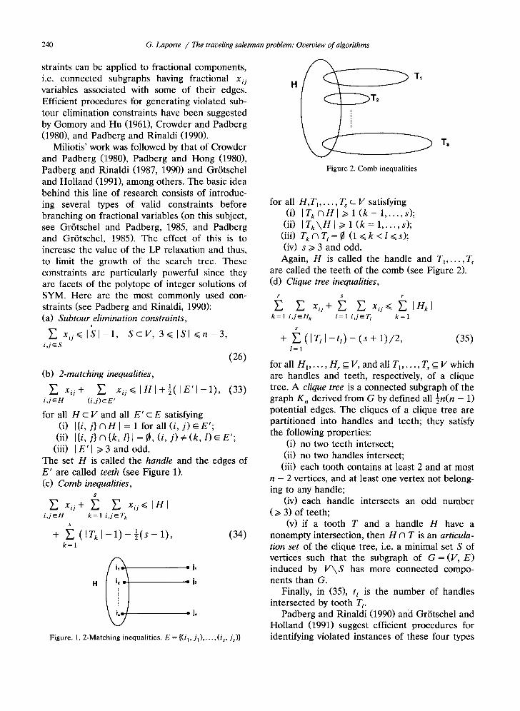
The set H is called the handle and the edges of E ' are called teeth (see Figure 1). (c) Comb inequalities,

E Xij"l- ~ E Xij< IHI i,j~H k = l i,j~T k

+ ~ ( I T k l - - 1 ) - - ½ ( s - - 1 ) , (34) k = l

H i~ =! • h

• j ,

Figure. 1 .2 -Match ing inequalities. E = {(il, J l) . . . . . (is, Js)}

H T1

. .• Ts J

Figure 2. Comb inequalit ies

for all H, T1, . . . , T s c V satisfying (i) IT k A H I > / 1 ( k = 1 . . . . . s);

(ii) [ T ~ \ H [ > t l ( k = l . . . . ,s); (iii) T k A T t = ¢ ( l ~ k < l ~ < s ) ; (iv) s >1 3 and odd.

Again, H is called the handle and T t . . . . . T s are called the teeth of the comb (see Figure 2). (d) Clique tree inequalities,

k = l i,j~H k t = l i,j~T t k = l

+ ~ (IT, I - t t ) - (s + 1) /2 , (35) l=1

for all H~ . . . . , H r c_ V, and all T 1 . . . . . Ts _c V which are handles and teeth, respectively, of a clique tree. A clique tree is a connected subgraph of the graph K n derived from G by defined all Xn(n - 1) potential edges. The cliques of a clique tree are partitioned into handles and teeth; they satisfy the following properties:

(i) no two teeth intersect; (ii) no two handles intersect;

(iii) each tooth contains at least 2 and at most n - 2 vertices, and at least one vertex not belonging to any handle;

(iv) each handle intersects an odd number (>/3) of teeth;

(v) if a tooth T and a handle H have a nonempty intersection, then H n T is an articula- tion set of the clique tree, i.e. a minimal set S of vertices such that the subgraph of G = (V, E) induced by V \ S has more connected components than G.

Finally, in (35), t t is the number of handles intersected by tooth T t.

Padberg and Rinaldi (1990) and Gr6tschel and Holland (1991) suggest efficient procedures for identifying violated instances of these four types

G. Laporte / The traveling salesman problem: Overview of algorithms

of constraints. By incorporating these procedures within an ILP code, these authors have solved to optimality TSPs containing between 17 and 2392 vertices. At time of writing, the 2392-vertex problem is believed to be the largest nonrandom symmetrical TSP ever solved to optimality.

5. H e u r i s t i c a l g o r i t h m s

Since the TSP is a NP-hard problem, it is natural to tackle it by means of heuristic algorithms. One stream of research has consisted of developing heuristics with a guaranteed worst-case performance. Most effort has, however, been de- voted to the design of heuristics with good empirical performance. In this section, we examine these two streams.

5.1. Heuristics with guaranteed worst-case performance

Consider a symmetrical TSP defined on a graph G and where C satisfies the triangle inequality. Let z * be the value of the optimal TSP solution. A simple way to derive a lower bound on z * is to first compute the length of a shortest spanning tree T on G. As shown by Aho, Hopcroft and Ullman (1974), this can be done in O(n 2) time. Denote by l(T) the length of that tree. A possible strategy for visiting all vertices is to traverse the spanning tree along its edges in the following fashion:

Step 1 Consider any leaf i 0 (vertex of degree 1) of the spanning tree and set i := i 0.

Step 2 - If there is any untraversed edge (i, j ) inci-

dent to vertex i, follow that edge to vertex j. Set i := j and repeat Step 2. - If all edges from vertex i have already been traversed, go back to the vertex k from which i was first reached. If k = i0, stop; otherwise set k .'= i and repeat Step 2.

In order to illustrate this procedure, consider the spanning tree depicted in Figure 3. Starting with i 0 = 1, one then proceeds to 3, 2, 3, 4, 5, 6, 5, 8, 5, 7, 5, 4, 3 and 1. It is easy to see that every edge of the spanning tree is then covered exactly twice. In general, this solution is not a tour. In

241

1 2 1 2

4- 5 6 4 5 6

7 ~ 8 8 Figure 3. Optimal traversal of a graph using a shortest span-

ning tree

order to obtain a tour, the above procedure must be modified by using shortcuts. Follow the path obtained, but skip any already visited vertex. In our example, one would follow the path (1, 3, 2, 4, 5, 6, 8, 7, 1). Since the triangle inequality is satisfied, this never increases the total distance traveled and moreover, the resulting closed path is a tour of length not exceeding 2/ (T) ~< 2z*

Christofides (1976) has proposed an improvement to the above procedure. It is based on the following observation. The shortest spanning tree is not in general Eulerian. However, an Eulerian graph can be derived from it by linking its odd- degree vertices by means of a minimum-cost matching algorithm. This can be done in O(n 3) time (Papadimitriou and Steiglitz, 1982). New edges corresponding to the optimal matching solution are then appended to the tree. Let l (M) denote their total length. The resulting graph is Eulerian and its complete traversal requires a total distance of I (T)+ l(M). Again, using shortcuts, a tour of total length not exceeding l(T) + l (M) can be obtained. This is illustrated in Figure 4. Figures 4a and 3a are identical. Figure 4b is obtained by solving a minimum-cost matching problem; the added edges are shown by the dashed lines. Traversing the resulting graph by

1 2 1 2

s 6 ""..s 6_

7 ~ 8 7 ~ " " 8 Figure 4. Optimal traversal of a graph using a shortest span-

ning tree and minimum matching


Figure 5. Christofides' heuristic

means of the above procedure can be done by following the path (1, 2, 3, 4, 5, 6, 8, 5, 7, 5, 3, 1). Using shortcuts yields the tour (1, 2, 3, 4, 5, 6, 8, 7, 1).

We now focus our attention on I(M). Consider the sequence of vertices on an optimal TSP tour and link by shortcuts all vertex pairs corresponding to edges in the optimal matching solutions; delete all in[ermediate vertices. The total length of these edges is I(M). Now close the tour by linking these edges in the same order as they appear on the tour (see Figure 5). The newly introduced edges have a total length of I(M')<~ I(M) since the first matching is optimal. Since I(M) + I(M') <~ z*, it follows that I(M) <~ z * / 2 and therefore, the heuristic yields a tour of length not exceeding I(T) + I(M) <~ 3z */2.

Finally, it should be mentioned that no heuristic with a guaranteed worst-case performance is known for the asymmetrical TSP.

5.2. Heuristics with good empirical performance

We now concentrate on a number of heuristics known to yield good TSP solutions in an empirical sense. Broadly speaking, TSP heuristics can be classical into tour construction procedures which involve gradually building a solution by adding a new vertex at each step, and tour improvement procedures which improve upon a feasible solution by performing various exchanges. The best methods are composite algorithms com- bining these two features. Most methods described in this section work on symmetrical and asymmetrical problems. There are, however, some exceptions that will be indicated. For further

readings on this subject, see Rosenkrantz, Stearns and Lewis (1977), Golden and Stewart (1985) and Ong and Huang (1989).

5.2.1. Tour construction procedures (a) The nearest-neighbour algorithm (Rosen- krantz, Stearns and Lewis, 1977).

In this method, a feasible tour is constructed by taking at each step the decision that is immediately the most advantageous. The main-interest of this 'myopic' algorithm lies in this simplicity.

Step 1. Consider an arbitrary vertex as a starting point.

Step 2. Determine the closest vertex to the last vertex considered and include it in the tour. If any vertex has not yet been considered, repeat Step 2.

Step 3. Link the last vertex of the tour to the first one.

The complexity of this procedure is O(n2). A possible modification is to consider in turn all n vertices as a starting point. The overall algorithm complexity is then O(n3), but the resulting tour is generally better. (b) Insertion algorithms (Rosenkrantz, Stearns and Lewis, 1977; Stewart, 1977; Norback and Love, 1977, 1979; Or, 1976).

This category includes a number of similar algorithms whose basic structure can be summarized as follows:

Step 1. Construct a first tour consisting of two vertices.

Step 2. Consider in turn all vertices not yet in the tour. Insert in the tour a vertex chosen with respect to a given criterion, for example: - the vertex yielding the least distance incre-

ment; - the vertex closest to the current tour; - the vertex furthest away from the tour; - the vertex forming the largest angle with two

consecutive vertices of the tour, etc.

Depending on the criterion that is used, the complexity of this type of procedure varies between O(n 2) and O(n log n). (c) The patching algorithm for asymmetrical TSPs (Karp, 1979).

G. Laporte / The traeeling salesman problem: Overview of algorithms 243

Figure 6. Merging two subtours in the patching algorithm

The following procedure was devised by Karp for asymmetrical TSPs. It exploits the fact that on problems for which the cifs are uniformly distributed, the assignment relaxation of the TSP provides a near-optimal solution (see Balas and Toth, 1985).

Step 1. Solve the AP with cost matrix C. Step 2. If the solution contains only one circuit,

stop. Step 3. Select the two circuits having the largest

numbers of vertices. Select an arc (i, j ) on the first circuit and an arc (k, l) on the second circuit that minimize the cost Cil q- Ckj -- Cij -- Ckl of

merging the two circuits (see Figure 6). Go to Step 2.

5.2.2. Tour improuement procedures These methods are used to improve a tour

obtained by any means. They will be classified into three main categories. (a) The r-opt algorithm (Lin, 1965).

Step 1. Consider an initial tour. Step 2. Remove r arcs from the tour and

tentatively reconnect the r remaining chains in all possible ways. If any reconnection yields a shorter tour, consider this tour as a new initial solution and repeat Step 2. Stop when no improvement can be obtained.

This heuristic was originally devised for symmetrical TSPs. In this case, the number of candi- date solutions at each step is of the order of n r since there are (~) ways to remove r arcs and r! ways to reconnect the resulting undirected chains. Not all these reconnections are, however, feasible. In general, r is taken as 2 or 3. One interesting exception is the Christofides and Eilon (1972) implementat ion of this method with r = 4 and 5.

Lin and Kerninghan (1973) have proposed an improvement to this method. Here, the value of r is modified dynamically throughout the algorithm. This procedure is considerably more diffi- cult to code than the original Lin r-opt method, but it generally produces near-optimal solutions. Recently Johnson (1990) has developed a "rando- mized iterated L in -Kern ingham method" that produces near-optimal solutions. Or (1976) has proposed a simplified exchange procedure requir- ing only O(n 2) operations at each step, but pro- ducing tours nearly as good on the average as those obtained with a 3-opt algorithm. Or 's algorithm can be described as follows:

Step 1. Consider an initial tour and set t := 1 and s := 3.

Step 2. Remove from the tour a chain of s consecutive vertices, starting with the vertex in position t, and tentatively insert it between all remaining pairs of consecutive vertices on the tour. - If the tentative insertion decreases the cost of

the tour, implement it immediately, thus defin- ing a new tour; set t := 1 and repeat Step 2.

- If no tentative insertion decreases the cost of the tour, set t := t + 1. If t = n + 1, then proceed to Step 3, otherwise repeat Step 2. Step 3. Set t : = l and s : = s - l . I f s > 0 , g o t o

Step 2; otherwise stop.

Before closing this section, it is worth mentioning that Kanellakis and Papadimitriou (1980) have suggested an adaptat ion of the Lin and Kernighan procedure to the asymmetrical case. According to the analysis of Golden and Stewart (1985), further experiments are required to confirm that this procedure is indeed competitive. (b) Simulated annealing (Kirkpatrick et al., 1983).

This successive improvements method is derived from an analogy with a m~terial annealing process used in mechanics (Metropolis et al., 1953). In order to bring a material to a minimal- energy solid state, it is necessary to heat it until its particles are randomly distributed in the liquid state; then, to avoid local minima, its tempera ture is gradually reduced in steps, until the system reaches an equilibrium step for a given tempera- ture level. At a high tempera ture T, all possible states can be reached but as the system cools down, the number of possibilities is reduced and the process converges to a stable state.

244 G. Laporte / The traveling salesman problem: Overuiew of algorithms

In combinatorial optimization, the aim is to move from a given initial solution to a minimum- cost solution, by performing gradual changes to the starting solution. Denote by T the state of the process (T corresponds to a tempera ture level in a physical system). In the beginning, the value of T is high and the number of allowed moves is also high. This number decreases with T, until no change to the solution is possible. A local minimum has then been reached.

For a given value of T, the algorithm is similar to the r-opt procedure: all solutions y in a neighbourhood of a solution x are examined. How- ever, substituting x by y is sometimes allowed even if this results in a larger cost. This reduces the probability of becoming t rapped in a local optimum. Simulated annealing can be applied to a large spectrum of combinatorial optimization problems. Formally, it can be summarized as follows:

Step 1. Consider an initial tour x of cost F(x). Step 2. Consider a solution y of cost F(y) in

the neighbourhood of x. If F ( y ) < F(x), set x := y and repeat Step 2. If F(y) >~ F(x), define Pr exp {[F(x) - F(y)]/T}, where T is a parameter tend- ing towards zero as the process evolves. Ran- domly select a number r in [0,1]. If r <~Pr, set x :=y and repeat Step 2. Otherwise, repeat Step 2 with a new solution y in the neighbourhood of x, or stop if this neighbourhood has been completely examined.

Simulated annealing has been applied to the TSP by a number of authors including Bonomi and Lutton (1984), Rossier, Troyon and Liebling (1986), Golden and Skiscim (1986) and Nahar, Sahni and Shragowitz (1989), with apparently a mixed degree of success. (c) Tabu search (Glover 1977, 1988, 1989, 1990; Glover and McMillan, 1986).

As in the previous two methods, successive neighbours of a solution x are examined and, as for simulated annealing, the objective is allowed to deteriorate in order to avoid local minima. In order to prevent - cycling, solutions that have already been examined are forbidden and inserted in a constantly updated ' tabu list'. The method can be summarized in three steps:

Step 1. Consider an initial solution x of cost F(x). Set the tabu list T := ~.

Step 2. Let N(x) be a neighbourhood of x. If N ( x ) \ T = ¢, go to Step 3. Otherwise, identify a least cost solution y in N ( x ) \ T and set x . '=y . Update T and the best known solution.

Step 3. If the maximum number of allowed iteractions since the beginning of the process or since the last update has been reached, stop. Otherwise, go to Step 2.

The success of this method depends on the careful choice of a number of control parameters. For more details on this, see Soriano (1989). Several authors have applied tabu search to the TSP (see Knox, 1988, Malek, 1988, and Fiechter, 1990) with seemingly very positive results.

5.2.3. Composite algorithms In recent years, two effective composite algo-

rithms have been developed. The first is the Golden and Stewart (1985) CCAO heuristic. The second, GENIUS, is more recent. It was devised by Gendreau, Hertz and Laporte (1990). (a) The CCAO algorithm (Golden and Stewart, 1985).

This heuristic was designed for symmetrical Euclidean TSPs. It exploits a well-known property of such problems, namely that in any optimal solution, vertices located on the convex hull of all vertices are visited in the order in which they appear on the convex hull boundary (Flood, 1956). The method can be summarized as follows:

Step 1 (C: convex hull). Define an initial (partial) tour by forming the convex hull of vertices.

Step 2 (C: cheapest insertion). For each vertex k not yet contained in the tour, identify the two adjacent vertices i k and jk on the tour such that Ci k k "~ Ck Jk -- Cik Jk is minimized.

'Step 3" (A: largest angle). Select the vertex k* that maximizes the angle between edges (ik, k) and (k, j~) on the tour, and insert it between ik. and Jk*-

Step 4 Repea t Steps 2 and 3 until a Hamilto- nian tour of all vertices is obtained.

Step 5 (O: Or-opt). Apply the Or-opt procedure to the tour and stop.

The rationale behind Steps 2 and 3 is that by selecting k * so as to maximize the angle it makes with the tour, the solution remains as close as possible to the initial convex hull.


(b) The GENIUS algorithm (Gendreau, Hertz and Laporte, 1992).

One major drawback of the CCAO algorithm is that its insertion phase is myopic in the following sense: since insertions are executed sequentially without much concern for global optimality, they may result in a succession of bad decisions that the post-optimization phase will be unable to undo. GENIUS executes each insertion more carefully, by performing a limited number of local transformation of the tour, simultaneously with the insertion itself. It consists of two parts: a generalized insertion phase, followed by a post- optimization phase that successively removes vertices from the tour and reinserts them, using the generalized insertion rule.

The algorithm has been extensively tested on randomly generated problems and on problems taken from the literature; all these problems were symmetrical and Euclidean. Tests revealed that GENIUS produces in shorter computing times better solutions than CCAO, itself superior to all tour construction heuristics developed in this section. This algorithm also appears to compare favourably to tabu search and simulated annealing, although the number of comparisons was more limited in the case of these two methods.

6. Conclusion

The TSP occupies a central place in Opera- tional Research. It underlies several practical applications and its study over the last 35 years or so has led to important theoretical developments. Problems involving a few hundred vertices can now be solved routinely to optimality. Instances involving more than 2000 vertices have also been solved exactly by means of constraint relaxation algorithms. A number of powerful heuristics have also been proposed: tabu search methods and generalized insertion algorithms appear to hold much potential.

Acknowledgements

This research was in part supported by the Canadian Natural Sciences and Engineering Re- search Council (grant OGP0039682), and by a Q u e b e c - N e w - Brunswick interprovincial re-

search grant. An extended version of this paper will appear in Discrete Optimization Models, H.A. Eiselt and C.L. Sandblom (eds.), De Gruyter, Berlin, 1993. Permission to publish this paper in EJOR is gratefully acknowledged. Finally, thanks are due to Paolo Toth for his valuable comments on a preliminary version of this paper.

References

Aho, A.V., Hopcroft, J.E., and Ullman, J.D. (1974), The Design and Analysis of Computer Algorithms, Addison- Wesley, Reading, MA.

Balas, E., Christofides, N. (1981), "A restricted lagrangean approach to the traveling salesman problem", Mathemati- cal Programming 21, 19-46.

Balas, E., Toth, P. (1985), "Branch and bound methods", in: E.L. Lawler, J.K. Lenstra, A.H.G. Rinnooy Kan and D.B. Shmoys (eds.), The Traveling Salesman Problem. A Guided Tour of Combinatorial Optimization, Wiley, Chichester, 361-401.

Bellmore, M., and Malone, J.C. (1971), "Pathology of traveling-salesman subtour-elimination algorithms", Operations Research 19, 278-307.

Bland, R.G., and Shallcross, D.F. (1989), "Large traveling salesman problems arising experiments in X-ray crystallography: A preliminary report on computation", Operations Research Letters 8, 125-128.

Bonomi, E., and Lutton, J.-L. (1984), "The N-city travelling salesman problem: Statistical mechanics an the Metropolis algorithm", SIAM Review 26, 551-568.

Carpaneto, G., Fischetti, M., and Toth, P. (1989), "'New lower bounds for the symmetric travelling salesman problem", Mathematical Programming 45,233-254.

Carpaneto, G., Martello, S., and Toth, P. (1988), "Algorithms and codes for the assignment problem", in: B. Simeone, P. Toth, G. Gallo, F. Maffioli, and S. Pallottino (eds.), FOR- TRAN Codes for Network Optimization, Annals of Opera- tions Research 13, 193-223.

Carpaneto, G., and Toth, P. (1980), "Some new branching and bounding criteria for the asymmetric travelling salesman problem", Management Science 26, 736-743.

Christofides, N. (1970), "The shortest Hamiltonian chain of a graph", SIAM Journal on Applied Mathematics 19, 689-696.

Christofides, N. (1976), "Worst-case analysis of a new heuristic for the travelling salesman problem", Report 388, Graduate School of Industrial Administration, Carnegie- Mellon University, Pittsburgh, PA.

Christofides, N., and Eilon, S. (1972). Algorithms for large- scale travelling salesman problems, Operational Research Quarterly 23, 511-518.

Crowder, H., and Padberg, M.W. (1980), "Solving large-scale symmetric travelling salesman problems to optimality", Management Science 26, 495-509.

Dantzig, G.B., Fulkerson, D.R., and Johnson, S.M. (1954), "Solution of a large-scale traveling-salesman problem", Operations Research 2, 393-410.


Dantzig, G.B., Fulkerson, D.R., and Johnson, S.M. (1954), "Solution of a large-scale traveling-salesman problem", Operations Research 2, 393-410.

Dantzig, G.B., Fulkerson, D.R., and Johnson, S.M. (1959), "On a linear-programming combinatorial approach to the traveling-salesman problem", Operations Research 7, 58- 66.

Desrochers, M., and Laporte, G. (1991), "Improvements and extensions to the Miller-Tucker-Zemlin subtour elimination constraints", Operations Research Letters 10, 27-36.

Eastman, W.L. (1958), "Linear programming with pattern constraints", Ph.D. Thesis, Harvard University, Cam- bridge, MA.

Eiselt, H.A., and Laporte, G. (1991), "A combinatorial optimization problem arising in dartboard design", Journal of the Operational Research Society 42, 113-118.

Fiechter, C.-N. (1990), "A parallel tabu search algorithm for large scale traveling salesman problems", Working Paper 90/1, D~partement de Math~matiques, lEcole Polytech- nique F6d6rale de Lausanne.

Fischetti, M., and Toth, P. (1991), "An additive bounding procedure for the asymmetric travelling salesman problem", Mathematical Programming, forthcoming.

Flood, M.M. (1956), "The traveling-salesman problem", Oper- ations Research 4, 61-75.

Garey, M.R., and Johnson, D.S. (1979), "Computers and intractability: A guide to the theory of NP-completeness", Freeman, San Francisco.

Garfinkel, R.S. (1973), "On partitioning the feasible set in a branch-and-bound algorithm for the asymmetric traveling-salesman problem", Operations Research 21, 340-343.

Garfinkel, R.S. (1977), "Minimizing wallpaper waste, Part I: A class of traveling salesman problems", Operations Re- search 25, 741-751.

Gavish, B., and Srikanth, K.N. (1986), "An optimal solution method for large-scale multiple traveling salesman problems", Operations Research 34, 698-717.

Gendreau, M. Hertz, A., and Laporte, G. (1992), "New insertion and post-optimization procedures for the traveling salesman problem", Operations Research, forthcoming.

Gilmore, P.C., and Gomory, R.E. (1964), "Sequencing a one state-variable machine: A solvable case of the traveling salesman problem", Operations Research 12, 655-679.

Gilmore, P.C., Lawler, E.L., and Shmoys, D.B. (1985), "Well- solved special cases", in: E.L. Lawler, J.K. Lenstra, A.H.G. Rinnooy Kan, and D.B. Shmoys (eds.), The Traveling Salesman Problem. A Guided Tour of Combinatorial Opti- mization, Wiley, Chichester, 87-143.

Glover, F. (1977), "Heuristic for integer programming using surrogate constraints",Decision Sciences 8, 156-166.

Glover, F. (1988), "Tabu search", Report 88-3, Center for Applied Artificial Intelligence (CAAI), Graduate School of Business, University of Colorado.

Glover, F. (1989), "Tabu search, Part I", ORSA Journal on Computing 1, 190-209.

Glover, F. (1990), "Tabu search", Part II, ORSA Journal on Computing 2, 4-32.

Glover, F., and McMillan, C. (1986), "The general employee scheduling problem: An integration of MS and AI", Com- puters & Operations Research 13, 563-573.

Golden, B.L., and Skiscim, C.C. (1986), "Using simulated annealing to solve routing and location problems", Naval Research Logistics Quarterly 33, 261-280.

Golden, B.L., and Stewart, Jr., W.R. (1985), "Empirical analysis of heuristics", in: E.L. Lawler, J.K. Lenstra, A.H.G. Rinnooy Kan, and D.B. Shmoys (eds.), The Traveling Salesman Problem. A Guided Tour of Combinatorial Opti- mization, Wiley, Chichester, 207-249.

Gomory, R.E. (1963), "An algorithm for integer solutions to linear program", in: R.L. Graves, and P. Wolfe (eds). Recent Advances in Mathematical Programming, McGraw- Hill, New York, 269-302.

Gomory, R.E., and Hu, T.C. (1961), "Multi-terminal network flows", SlAM Journal on Applied Mathematics 9, 551-556.

Gr6tschel, M., and Holland, O. (1991), "Solution of large-scale symmetric travelling salesman problems", Mathematical Programming 51, 141-202.

Gr6tschel, M., and Padberg, M.W. (1985), "Polyhedral theory", in: E.L. Lawler, J.K. Lenstra, A.H.G. Rinnooy Kan, and D.B. Shmoys (eds.), The Traveling Salesman Problem. A Guided Tour of Combinatorial Optimization, Wiley, Chichester, 251-305.

Helbig Hansen, K., and Krarup, J. (1974), "Improvements of the Held-Karp algorithm for the symmetric traveling-salesman problem", Mathematical Programming 7, 87-96.

Held, M., and Karp., R.M. (1970), "The traveling salesman problem and minimum spanning trees", Operations Re- search 18, 1138-1162.

Held, M., and Karp, R.M. (1971), "The traveling salesman problem and minimum spaning trees: Part II", Mathemati- cal Programming 1, 6-25.

Johnson, D.S. (1990), "Local optimization and the traveling salesman problem", in: M.S. Paterson (ed.), Proceedings of the 17th International Colloquium on Automata, Languages and Programming, Lecture Notes in Computer Science, Springer-Verlag, Berlin, 446-461.

Kanellakis, P.-C., and Papadimitriou, C.H. (1980), "Local search for the asymmetric traveling salesman problem", Operations Research 28, 1086-1099.

Karp, R.M. (1979), "A patching algorithm for the nonsymmet- ric traveling-salesman problem", SIAM Journal on Com- puting 8, 561-573.

Kirkpatrick, S., Gelatt, Jr., C.D., and Vecchi, M.P. (1983), "Optimization by simulated annealing", Science 220, 671- 680.

Knox, J. (1988), "An application of TABU search to the symmetric traveling salesman problem", Ph.D. Thesis, Center for Applied Artificial Intelligence (CAAI), Gradu- ate School of Business, University of Colorado.

Langevin, A., Soumis, F., and Desrosiers, J. (1990), "Classifi- cation of travelling salesman problem formulations", Oper- ations Research Letters 9, 127-132.

Laporte, G. (1992), "The vehicle routing problem: An overview of exact and approximate algorithms", European Journal of Operational Research, 59, 345-358 (to appear).


Lawler, E.L., Lenstra, J.K., Rinnooy Kan, A.H.G., and Shmoys, D.B. (1985), The Traveling Salesman Problem. A Guided Tour of Combinatorial Optimization, Wiley, Chich- ester.

Lenstra, J.K., Rinnooy Kan, A.H.G. (1975), "Some simple applications of the travelling salesman problem", Opera- tional Research Quarterly 26, 717-733.

Lin, S. (1965), "Computer solutions of the traveling salesman problem", Bell System Computer Journal 44, 2245-2269.

Lin, S., and Kernighan, B.W. (1973), "An effective heuristic algorithm for the traveling-salesman problem", Operations Research 21,498-516.

Little, J.D.C., Murty, K.G., Sweeney, D.W., and Karel, C. (1963), "An algorithm for the traveling salesman problem", Operations Research 11, 972-989.

Malek, M. (1988), "Search methods for traveling salesman problems", Working Paper, University of Texas, Austin, TX.

Martin, G.T. (1966), "Solving the traveling salesman problem by integer programming", Working Paper, CEIR, New York.

Metropolis, N., Rosenbluth, A.W., Rosenbluth, M.N., Teller, A.H., and Teller, E. (1953), "Equation of state calcula- tions by fast computing machines", Journal of Chemical Physics 21, 1087-1091.

Miliotis, P. (1976), "Integer programming approaches to the travelling salesman problem", Mathematical Programming 10, 367-378.

Miliotis, P. (1978), "Using cutting planes to solve the symmetric salesman problem", Mathematical Programming 15, 177-188.

Miller, D.L., and Pekny, J.F. (1989), "Results from a parallel branch and bound algorithm for solving large asymmetric traveling salesman problems", Operations Research Letters 8, 129-135.

Miller, D.L., and Pekny, J.F. (1991), "Exact solution of large asymmetric traveling salesman problems", Science 251, 754-761.

Miller, C.E., Tucker, A.W., and Zemlin, R.A. (1960), "Integer programming formulations and traveling salesman problems", Journal of the Association for Computing Machinery 7, 326-329.

Murty, K.G. (1968), "An algorithm for ranking all the assign- ments in order of increasing cost", Operations Research 16, 682-687.

Nahar, S., Sahni, S., and Shragowitz, E. (1989), "Simulated annealing and combinatorial optimization", International Journal of Computer Aided VLSI Design 1, 1-23.

Norback, J., and Love, R. (1977), "Geometric approaches to solving the traveling salesman problem", Management Sci- ence 23, 1208-1223.

Norback, J., and Love, R. (1979), "Heuristic for the Hamilto- nian path problem in Euclidean two space", Journal of the Operational Research Society 30, 363-368.

Ong, H.L., and Huang, H.C. (1989), "Asymptotic expected performance of some TSP heuristics", European Journal of Operational Research 43, 231-238.

Or, I. (1976), "Traveling salesman-type combinatorial prob-

lems and their relation to the logistics of regional blood banking", Ph.D. Dissertation, Northwestern University, Evanston, IL.

Padberg, M.W., and Gr6tschel, M. (1985), "Polyhedral computations", in: E.L. Lawler, J.K. Lenstra, A.H.G. Rinnooy Kan, and D.B. Shmoys (eds.), The Traveling Salesman Problem. A Guided Tour of Combinatorial Optimization, Wiley, Chichester, 307-360.

Padberg, M.W., and Hong, S. (1980), "On the symmetric traveling salesman problem: A computational study", Mathematical Programming Study 12, 78-107.

Padberg, M.W., and Rinaldi, G. (1987), "Optimization of a 532-city symmetric traveling salesman problem by branch and cut", Operations Research Letters 6, 1-7.

Padberg, M.W., and Rinaldi, G. (1990), "Facet identification for the symmetric traveling salesman problem", Mathemat- ical Programming 47, 219-257.

Papadimitriou, C.H., and Steiglitz, K. (1982), Combinatorial Optimization: Algorithms and Complexity, Prentice-Hall, Englewood Cliffs, NJ.

Reinelt, G. (1989), "Fast heuristics for large geometric traveling salesman problems", Report No. 185, Institut fiir Mathematik, Universit~it Augsburg.

Rosenkrantz, D.J., Stearns, R.E., and Lewis, II, P.M. (1977), "An analysis of several heuristics for the traveling salesman problem", SIAM Journal on Computing 6, 563-581.

Rossier, Y., Troyon, M., and Liebling, T.M. (1986), "Prob- abilistic exchange algorithms and the Euclidian traveling salesman problem", Operations Research Spektrum 8, 151- 164.

Shapiro, D.M. (1966), "Algorithms for the solution of the optimal cost and bottleneck traveling salesman problems", Sc.D. Thesis, Washington University, St. Louis, MO.

Smith, T.H.C., Srinivasan, V., and Thompson, G.L. (1977), "Computational performance of three subtour elimination algorithms for solving asymmetric traveling salesman problems", Annals of Discrete Mathematics 1,495-506.

Smith, T.H.C., and Thompson, G.L. (1977), "A LIFO implicit enumeration search algorithm for the symmetric traveling salesman problem using Held and Karp's 1-tree relaxation", Annals of Discrete Mathematics 1, 479-493.

Soriano, P. (1989), "l~tude de nouvelles avenues de recherche propos~es en optimisation combinatoire", Publication CRT-619, Centre de recherche sur les transports, Montr6al.

Stewart, Jr., W.R. (1977), "A computationally efficient heuristic for the traveling salesman problem", Proceedings of the 13th Annual Meetings of S.E. Tims, 75-85.

Tarjan, R.E. (1977), "Finding optimum branchings", Net- works 7, 25-35.

Volgenant, T., and Jonker, R. (1982), "A branch and bound algorithm for the symmetric traveling salesman problem based on the 1-tree relaxation", European Journal of Oper- ational Research 9, 83-89.

Wong, R.T. (1980), "Integer programming formulations of the travelling salesman problem", Proceedings of the IEEE International Conference on Circuits and Computers, 149- 152.

an overview of exact and approximate algorithms

Documents