an overview of nested decomposition for multi-level
TRANSCRIPT
An Overview of Nested Decomposition for
Multi-Level Optimization Problems
Stephen J. Maher1 and Ibrahim Muter2
1College of Engineering, Mathematics and Physical Sciences,University of Exeter, Exeter, United Kingdom
2Amazon Web Services, re:Invent Building, Seattle, WA 98121, USA
Abstract
Nested multi-level structures are frequently encountered in manyreal-world optimization problems. Decomposition techniques are acommonly applied approach used to handle nested multi-level struc-tures; however, the typical problem-specific focus of such techniqueshas led to numerous specialized formulations and solution methods.This lack of generalized results for nested multi-level optimizationproblems is addressed in this paper with the proposal of a theoreti-cal framework for their formulation and the application of decomposi-tion techniques. The developed theoretical framework will be used tohighlight the prevalence of general multi-level structures within a widerange of application areas. Further, state-of-the-art solution methodsfor nested multi-level optimization problems will be described in thecontext of the proposed framework. The discussion in this paper willhighlight the broad applicability of the general formulation and so-lution methodologies developed for this important class of real-worldoptimization problems.Key words: two-level decomposition; multi-level decomposition; col-umn generation; branch-and-price; integer programming.
1 Introduction
Structure, either mathematical or physical, is a common characteristic oflarge-scale optimization problems. This is due in part to the desire of opti-mization experts to introduce structure into mathematical models of large-scale systems, but also due to real-world problems typically exhibiting aphysical relationship between the components of the system being modeled.Classical examples of structure in large-scale optimization problems are theroutes in vehicle routing problems (VRP) that are independent for each vehi-cle but are linked for planning at the depot level or the independence of the
1

production schedules for each generator in the unit commitment problemthat must satisfy the demand at a network level. Aggregation is a com-mon feature of such problems where the individual base units are combinedto form an operational structure. The modeling approaches and solutionmethodologies for handling such aggregation are the primary concerns ofthis paper.
Consider a mathematical optimization problem given by
minimize cx, (1a)
subject to Ax ≥ b, (1b)
x ∈ {0, 1}n. (1c)
We consider the case of problem (1) where c is positive and the constraintmatrix A exhibits some structure. Further, we assume that this structurecan be exploited through the application of decomposition techniques, suchas Dantzig-Wolfe reformulation, Benders’ decomposition or Lagrangian re-laxation. While problems can exhibit a structure where many different de-composition techniques can be applied, we will focus primarily on problemstructures that are amenable to the application of Dantzig-Wolfe reformu-lation.
Formally, the structure that we wish to exploit is the following: Considern sets denoted by Ii for i ∈ {1, 2, . . . , n}. We describe the set I1 as the firstlevel, I2 the second level and so on. The elements in these sets are binaryvectors of length |Ii−1|. The basic units that are aggregated in levels Ii fori > 1 are contained in I1. The sets can be defined as Ii ⊆ {x | Ci(x) = 1, x 6=0, x ∈ {0, 1}|Ii−1|} for i ∈ {2, 3, . . . , n}, where Ci(x) = 1 indicates that xsatisfies all the conditions defined by Ci in level i. In the mathematicalprogramming context Ci can be a set of inequalities. For x ∈ Ii, i > 1,xj = 1 if the element indexed by j in Ii−1 is included in the aggregationgiven by x. This leads to the definition of a nested multi-level optimizationproblem:
Definition 1 A nested multi-level optimization problem is a problem inwhich for any N ∈ {2, . . . , n} there exists a formulation where each leveli < N is a subproblem for level i + 1. The goal of this problem is to find aselection of elements I ⊆ IN that minimizes
∑k∈I ckxk.
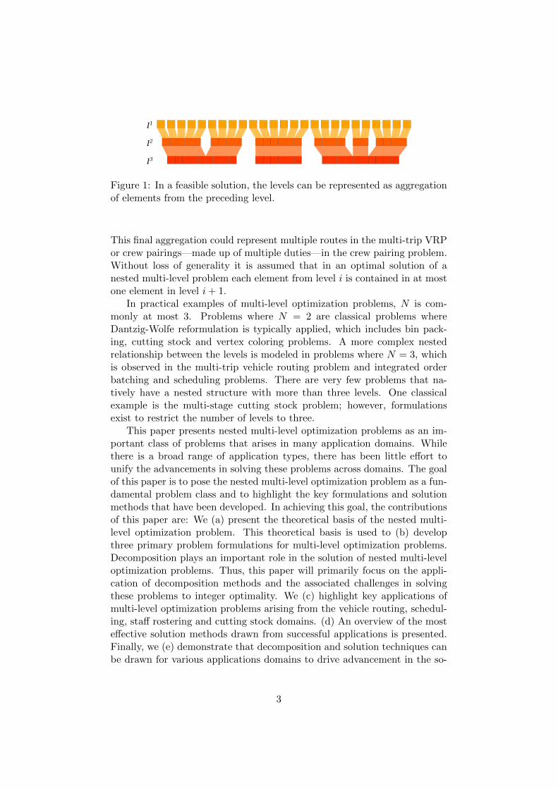
The nested multi-level structure is exemplified in Figure 1. This is an ex-ample of a feasible solution of a multi-level optimization problem. The firstlevel, I1 are the base elements of the optimization problem, such as cus-tomer locations in the VRP or flights in the airline crew pairing problem. Inthe second level, I2, these base elements are aggregated to form an orderedset satisfying the conditions C2. These aggregations could be vehicle routesvisiting multiple customers or crew duties comprised of a sequence of flights.The second level elements are then aggregated further in the third level, I3.
2
I1
I2
I3
Figure 1: In a feasible solution, the levels can be represented as aggregationof elements from the preceding level.
This final aggregation could represent multiple routes in the multi-trip VRPor crew pairings—made up of multiple duties—in the crew pairing problem.Without loss of generality it is assumed that in an optimal solution of anested multi-level problem each element from level i is contained in at mostone element in level i+ 1.
In practical examples of multi-level optimization problems, N is com-monly at most 3. Problems where N = 2 are classical problems whereDantzig-Wolfe reformulation is typically applied, which includes bin pack-ing, cutting stock and vertex coloring problems. A more complex nestedrelationship between the levels is modeled in problems where N = 3, whichis observed in the multi-trip vehicle routing problem and integrated orderbatching and scheduling problems. There are very few problems that na-tively have a nested structure with more than three levels. One classicalexample is the multi-stage cutting stock problem; however, formulationsexist to restrict the number of levels to three.
This paper presents nested multi-level optimization problems as an im-portant class of problems that arises in many application domains. Whilethere is a broad range of application types, there has been little effort tounify the advancements in solving these problems across domains. The goalof this paper is to pose the nested multi-level optimization problem as a fun-damental problem class and to highlight the key formulations and solutionmethods that have been developed. In achieving this goal, the contributionsof this paper are: We (a) present the theoretical basis of the nested multi-level optimization problem. This theoretical basis is used to (b) developthree primary problem formulations for multi-level optimization problems.Decomposition plays an important role in the solution of nested multi-leveloptimization problems. Thus, this paper will primarily focus on the appli-cation of decomposition methods and the associated challenges in solvingthese problems to integer optimality. We (c) highlight key applications ofmulti-level optimization problems arising from the vehicle routing, schedul-ing, staff rostering and cutting stock domains. (d) An overview of the mosteffective solution methods drawn from successful applications is presented.Finally, we (e) demonstrate that decomposition and solution techniques canbe drawn for various applications domains to drive advancement in the so-
3
lution of real-world multi-level optimization problems.This paper is organized as follows: Section 2 presents the theoretical
basis of multi-level optimization problems proposed in this paper and ageneric approach to modeling such problems. Importantly, various methodsfor decomposing nested multi-level optimization problems are presented inSection 2. The multi-trip vehicle routing problem (MTVRP) and multi-stage cutting stock problem (MSCS) will be used as examples in Section 2.5to illustrate the key aspects of the modeling and decomposition of nestedmulti-level optimization problems. In Section 3, we review the literature onproblems that are amenable to multi-level decomposition. Various solutionmethodologies used to solve the practical applications described in Section3 will be analyzed and discussed in Section 4. Section 5 will present somefinal remarks and directions for future research.
2 Two-level Decomposable Optimization Problem
In this section, and throughout this paper we will focus on a three-levelnested optimization problem. First, to guide the discussion, we formallydefine an N−level decomposable optimization problem as
Definition 2 An N -level decomposable optimization problem is a multi-level optimization problem with at least N + 1 levels, and this multi-levelstructure can be exploited by the application of decomposition methods.
By Definition 2, for a multi-level optimization problem with n+ 1 levels,it is possible to apply decomposition methods to exploit 1, 2, . . . , n levels.The resulting decompositions are described as a one-level, two-level, . . .,n−level decomposition respectively.
2.1 Exploiting problem structure
The corresponding form of (1) exhibiting the structure amenable to theapplication of Dantzig-Wolfe reformulation is
minimize cx, (2a)
subject to Ax ≥ b, (2b)
Bx ≤ d, (2c)
Ex ≤ f, (2d)
x ∈ {0, 1}n. (2e)
The matrix A is referred to as the Linking or Master Block and the matricesB and E are commonly referred to as subsystem blocks. It is common for Band E to exhibit a block-diagonal structure, where each system is disjointand linked through the constraints given by A. However, in a multi-level op-timization problem B may also provide a linking between the disjoint blocks
4

of E. The application of Dantzig-Wolfe reformulation results in a masterproblem consisting of the linking constraints and corresponding variables.The subproblems comprise the variables and constraints of each disjointblock. We will show in this section that the application of Dantzig-Wolfereformulation results in different formulations based upon the selection ofconstraints that comprise the master and subproblems.
An important feature of Dantzig-Wolfe reformulation is that the vari-ables in the master problem are a reformulation of the original variables.Problem (2) represents a problem with multiple levels, where C2(x) :=Bx ≤ d and C3(x) := Ex ≤ f . Consider the feasible region given byI2 = {x ∈ {0, 1}n|Bx ≤ d}, which we assume is a bounded polytope. Allfeasible solutions in I2 can be written as an integer combination of points{xq}q∈Q, which is given by
x =∑q∈Q
xqλq,∑q∈Q
λq = 1, λ ∈ Z|Q|+ , (3)
where Q is a finite set. The variables λq are implicitly restricted to binaryvariables and indicate whether the column given by the feasible solution xq
is selected. Upon substituting (3) into (2), this reformulation provides a sep-aration of the master and subproblems by exploiting the structure exhibitedby A and subsequently B. This type of reformulation is described as thediscretization approach (Vanderbeck 2000). The ability to form the set I2,which comprises the constraints Bx ≤ d, is the basis for the resulting refor-mulation. It is also possible to define I2′ = {x ∈ {0, 1}n+|Bx ≤ d,Ex ≤ f}and perform a similar reformulation. Using I2 or I2′ to perform the reformu-lation of (1) results in a different structure of the master and subproblems.Exploiting these different reformulation possibilities is the main driver forthe solution approaches presented in this paper.
One may notice that the variable reformulation given by (3) replaces a setof constraints in the master problem with exponentially more variables thanin the original problem. The motivation for performing such a reformulationis that the discretization of the feasible region I2 potentially results in animproved bound on the LP relaxation of (1). A prominent method forhandling this significant increase in variables is to solve the master problemusing a column generation algorithm. Briefly, a column generation algorithmgenerates the necessary columns required in the optimal solution of a linearprogramming (LP) problem by solving a pricing subproblem.
Dantzig-Wolfe formulation and column generation are very popular math-ematical programming techniques that have been used to solve many prob-lems arising from practical applications. For more details regarding Dantzig-Wolfe reformulation and column generation, we refer to Desaulniers et al.(2005) and Lubbecke and Desrosiers (2005). Our interest in nested multi-level problems comes from the observation that numerous problems from
5
different application domains are amenable to Dantzig-Wolfe reformulationin more than one level. From the literature it is evident that care must betaken when modeling mathematical programs with nested multi-level struc-tures, particularly when considering the solution methodology. This paperwill provide guidance and insight into different formulations and the avail-able solution methodologies for nested multi-level decomposable problems.
2.2 First-level Decomposition
Typically there is no one unique method for applying Dantzig-Wolfe refor-mulation to problem (2). While different reformulations are possible, theeffectiveness of related solution algorithms is affected by the reformulationthat is applied. In the above section, a reformulation of the original prob-lem variables is achieved using the feasible solutions contained in I2. Inthis case, the binary operator C2(x) = 1 is equivalent to the system of in-equalities Bx ≤ d. While for such a problem type this is true in general,it is expected that such a reformulation will be most effective if Bx ≤ dinduces a well-structured set that lends itself to efficient optimization overthe polyhedron, such as network flow or knapsack problems.
We define I2 as above and apply the reformulation given by (3). Afterthe substitutions cq = cxq, eq = Exq and aq = Axq for q ∈ Q, the first-levelmaster problem, which we will refer to as MP1, can be written as
(MP1) minimize∑q∈Q
cqλq, (4a)
subject to∑q∈Q
aqλq ≥ b, (4b)
∑q∈Q
eqλq ≤ f, (4c)
∑q∈Q
λq = 1, (4d)
λq ∈ Z+, q ∈ Q. (4e)
Constraints (4b) and (4c) correspond to the constraint sets (2b) and (2d) re-spectively. These constraints have been reformulated as a result of applyinga Dantzig-Wolfe reformulation. The constraint (4d) is the convexity con-straint that assures exactly one column satisfying (4b) and (4c) is selected.In many applications of decomposition, this constraint is omitted from themodel without affecting the optimal solution.
2.3 Second-level Decomposition
Suppose that∑
q∈Q eqλq ≤ f also has a structure that stimulates decompo-sition for the second time. This further decomposition will be referred to
6

as the second-level decomposition. The solution set that satisfies the con-straints (4c) and (4e) can be represented as I3 = {λ ∈ Z+|
∑q∈Q
eqλq ≤ f}.
Once again, we assume that the polytope I3 is bounded. The index set of allfeasible solutions contained in I3 is denoted by S and λs = [λs1 λ
s2 .. λ
s|Q|]
T
denotes the associated solutions. Let the variable ys equal 1 to indicatewhether the associated solution λs is selected, and 0 otherwise. After thesubstitutions cs =
∑q∈Q
cqλsq, as =
∑q∈Q
aqλsq for s ∈ S, the second-level master
problem, which we will refer to as MP2, can be written as
(MP2) minimize∑s∈S
csys, (5a)
subject to∑s∈S
asys ≥ b, (5b)∑s∈S
ys = 1, (5c)
ys ∈ Z+, s ∈ S. (5d)
Following the application of Dantzig-Wolfe reformulation to MP2, manysimilarities can be observed when comparing with MP1. In particular, thelarge cardinality of S makes solving MP2 using a general purpose solverimpractical. Column generation is then employed to dynamically generatevariables by first forming a restricted master problem by replacing S withS ⊆ S. However, because a two-level decomposition has been performed,the classical column generation approaches may not be computationally ef-fective. A discussion of variants to the classical column generation approachused to solve MP2 will be presented in Section 4.
As explained in the previous section, the first-level decomposition mustperform an aggregation of I1 into elements of I2. Thus, the set I3 wouldnot be achieved in the first-level decomposition due to the hierarchy betweenthe solution sets I1 and I2. Hence, it is not a matter of choice in the firstlevel to apply decomposition on Bx ≤ b or Ex ≤ f , i.e., the levels ofthe decomposition are not interchangeable. The illustrative examples inSection 2.5 will demonstrate the order dependency in the application ofdecomposition techniques on the original and master problems.
On the other hand, the constraint set (2d) can be included in the first-level decomposition by defining I2′ = {x ∈ {0, 1}n|Bx ≤ d,Ex ≤ f}. Thisapproach simultaneously decomposes both constraints sets that were decom-posed in the first- and second-level decomposition. Though this reformula-tion is not as prevalent as applying both levels of decomposition, it will pavethe way for a specific solution method.
7
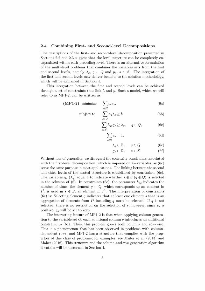
2.4 Combining First- and Second-level Decompositions
The descriptions of the first- and second-level decomposition presented inSections 2.2 and 2.3 suggest that the level structure can be completely en-capsulated within each preceding level. There is an alternative formulationof the multi-level problems that combines the variables sets from the firstand second levels, namely λq, q ∈ Q and ys, s ∈ S. The integration ofthe first and second levels may deliver benefits to the solution methodology,which will be explained in Section 4.
This integration between the first and second levels can be achievedthrough a set of constraints that link λ and y. Such a model, which we willrefer to as MP1-2, can be written as:
(MP1-2) minimize∑s∈S
csys, (6a)
subject to∑q∈Q
aqλq ≥ b, (6b)
∑s∈S
hqsys ≥ λq, q ∈ Q, (6c)∑s∈S
ys = 1, (6d)
λq ∈ Z+, q ∈ Q, (6e)
ys ∈ Z+, s ∈ S. (6f)
Without loss of generality, we disregard the convexity constraints associatedwith the first-level decomposition, which is imposed on λ−variables, as (6c)serve the same purpose in most applications. The linking between the secondand third levels of the nested structure is established by constraints (6c).The variables yp (λq) equal 1 to indicate whether s ∈ S (q ∈ Q) is selectedin the solution of (6). In constraints (6c), the parameter hqs indicates thenumber of times the element q ∈ Q, which corresponds to an element inI2, is used in s ∈ S, an element in I3. The interpretation of constraints(6c) is: Selecting element q indicates that at least one element s that is anaggregation of elements from I2 including q must be selected. If q is notselected, there is no restriction on the selection of s; however, since cs ispositive, ys will be set to zero.
The interesting feature of MP1-2 is that when applying column genera-tion to the variable set Q, each additional column q introduces an additionalconstraint to (6c). Thus, this problem grows both column- and row-wise.This is a phenomenon that has been observed in problems with column-dependent rows, and MP1-2 has a structure that complies with the prop-erties of this class of problems, for examples, see Muter et al. (2013) andMaher (2016). This structure and the column-and-row generation algorithmit entails will be discussed in Section 4.
8

As mentioned previously, an advantage of applying Dantzig-Wolfe refor-mulation is that it can result in an improved bound on the LP relaxation of(1). Since problem MP1-2 convexifies both the I2 and I3 feasible regions,there is no additional gain in the bound for the LP relaxation comparedto MP2. Thus, the choice to apply the decomposition of the form MP2or MP1-2 is dependent on the problem structure and the expectation ofsolution algorithm effectiveness.
2.5 Illustrative Examples
We exemplify the steps of the two-level decomposition and the resultingmodels using MTVRP and MSCS. The MTVRP is a variant of the classicalvehicle routing problem where each vehicle is allowed to perform more thanone route during the workday. In this problem, there exists a set of identicalvehicles, indexed by k ∈ K, located at a single depot. Each vehicle k hasa capacity D. The vehicles are used to satisfy the demands of a set ofcustomers, indexed by i ∈ I1. A vehicle k has a maximum driving time T ,and by that time it should end its schedule at the depot.
The MTVRP can be represented on a complete directed graph G =(N,A), where N = {0}∪I1 is the set of nodes comprising the depot indexedas 0 and the set of customers I1. There exists a demand of size di associatedwith each customer i ∈ I1. An arc (i, j) ∈ A is defined between each pairof nodes with an associated cost cij , which corresponds to time. A vehicleroute is given by a path formed by a set of arcs that originates from thedepot, visits a set of nodes and returns back to the depot. Additionally, aroute is only valid if the total demand of the customers to be visited does notexceed the capacity of the vehicle. The time required to complete all routesassigned to a vehicle must not exceed T . A set of routes R is associated witheach vehicle k ∈ K, and the variables xrkij are defined to equal 1 if arc (i, j)is traversed in route r ∈ R by vehicle k. The objective of the MTVRP is tofind a set of routes and its assignment to a number of vehicles such that the
9
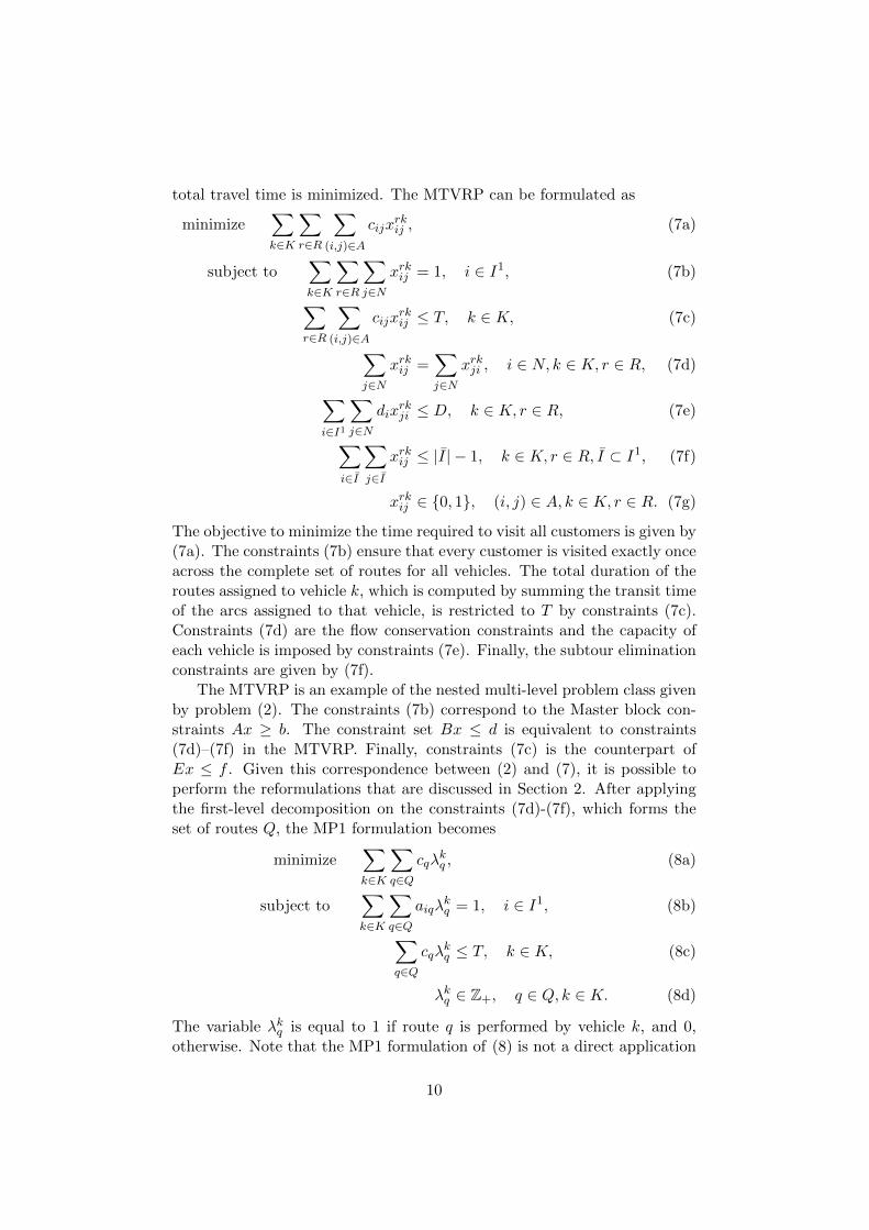
total travel time is minimized. The MTVRP can be formulated as
minimize∑k∈K
∑r∈R
∑(i,j)∈A
cijxrkij , (7a)
subject to∑k∈K
∑r∈R
∑j∈N
xrkij = 1, i ∈ I1, (7b)
∑r∈R
∑(i,j)∈A
cijxrkij ≤ T, k ∈ K, (7c)
∑j∈N
xrkij =∑j∈N
xrkji , i ∈ N, k ∈ K, r ∈ R, (7d)
∑i∈I1
∑j∈N
dixrkji ≤ D, k ∈ K, r ∈ R, (7e)
∑i∈I
∑j∈I
xrkij ≤ |I| − 1, k ∈ K, r ∈ R, I ⊂ I1, (7f)
xrkij ∈ {0, 1}, (i, j) ∈ A, k ∈ K, r ∈ R. (7g)
The objective to minimize the time required to visit all customers is given by(7a). The constraints (7b) ensure that every customer is visited exactly onceacross the complete set of routes for all vehicles. The total duration of theroutes assigned to vehicle k, which is computed by summing the transit timeof the arcs assigned to that vehicle, is restricted to T by constraints (7c).Constraints (7d) are the flow conservation constraints and the capacity ofeach vehicle is imposed by constraints (7e). Finally, the subtour eliminationconstraints are given by (7f).
The MTVRP is an example of the nested multi-level problem class givenby problem (2). The constraints (7b) correspond to the Master block con-straints Ax ≥ b. The constraint set Bx ≤ d is equivalent to constraints(7d)–(7f) in the MTVRP. Finally, constraints (7c) is the counterpart ofEx ≤ f . Given this correspondence between (2) and (7), it is possible toperform the reformulations that are discussed in Section 2. After applyingthe first-level decomposition on the constraints (7d)-(7f), which forms theset of routes Q, the MP1 formulation becomes
minimize∑k∈K
∑q∈Q
cqλkq , (8a)
subject to∑k∈K
∑q∈Q
aiqλkq = 1, i ∈ I1, (8b)
∑q∈Q
cqλkq ≤ T, k ∈ K, (8c)
λkq ∈ Z+, q ∈ Q, k ∈ K. (8d)
The variable λkq is equal to 1 if route q is performed by vehicle k, and 0,otherwise. Note that the MP1 formulation of (8) is not a direct application
10

of Dantzig-Wolfe reformulation described in Section 2.1. This can be seen bythe elimination of the r index and the omission of the convexity constraint.While it is possible to include these two aspects in the formulation, they areredundant.
An interesting feature of problem (8) is the knapsack structure in (8c),which can be further exploited through a second-level decomposition. Acombination of vehicle routes satisfying this constraint set, which is sepa-rable for each vehicle k, constitutes a vehicle schedule. Observe that (7c)exhibited this block diagonal structure also in the original formulation. How-ever, from the two-level decomposition perspective, it is impossible to rep-resent solutions satisfying constraints associated with the schedules beforethe route set Q is identified. Hence, the decomposition of constraints (7c) isdeferred to the second level of the decomposition. The second-level decom-position results in the MP2 formulation as follows:
minimize∑s∈S
csys, (9a)
subject to∑s∈S
aisys ≥ 1, i ∈ I1, (9b)∑s∈S
ys ≤ |K|, (9c)
ys ∈ {0, 1}, s ∈ S, (9d)
where S is the set of schedules, which are the aggregation of routes q ∈ Qsubject to the constraints imposed in the nested structure. The binaryvariable ys is defined to equal to 1 only if schedule s is selected. Sincevehicles are identical and a vehicle is not required to perform a schedule, theconvexity constraints take the form of (9c). This model could be achievedby defining I2′ as the set of solutions satisfying (7c)-(7g) in the first level ofdecomposition applied to problem (7). However, as mentioned previously,even though applying two-level decomposition and defining I2′ in a onelevel decomposition leads to the same formulation of the master problem,the solution methods and pricing subproblems will differ due to the numberof levels and constraints involved in the decomposition process.
An alternative model can be obtained by combining the first- and second-level decomposition to form MP1-2, as explained in Section 2.4. Due to theresemblance between problem (6) and this alternative model for solving theMTVRP, we refrain from repetition, and explain the analogy as follows:Constraint set (6b) in MTVRP ensures that each customer i ∈ I1 is visitedin exactly one route. Binary parameter hqs, as defined in MP1-2, equals 1only if route q ∈ Q is performed as part of schedule s ∈ S. Constraint set(6c) in this problem imposes that if a route q ∈ Q is selected, it must beperformed in at least one vehicle schedule. This formulation bears an algo-rithmic and computational burden in terms of the number of constraints in
11

(6c) when column generation is applied to two-level decomposable problems.Hence, MP1-2 is not a prevalent formulation in most application areas. Anexception is the MSCS, which exemplifies the case where tackling MP1-2can be preferable over MP2. The benefits of the MP1-2 formulation andits relationship with MP2 will be addressed and generalized based on theMSCS in Section 4. In the following, we present the problem description ofthe MSCS and its MP1-2 formulation.
Unlike the conventional cutting stock problem, MSCS arises when thestock roll cannot be cut directly into the finished rolls i ∈ I1, each identifiedby width ci. In this setting, a stock roll is first cut into intermediate rollswhose width is restricted to be within the interval [tmin, tmax]. These in-termediate rolls are then cut into finished rolls with a certain width, whichis based on demand. The first level decomposition forms the finished rollcutting pattern set I2, which are cut from intermediate rolls j ∈ J . In thesecond level, intermediate roll cutting patterns that are cut from the stockroll are defined in set I3. Adhering to the set notation and definitions givenin the previous section, we define Q and S as the sets of finished roll andintermediate roll patterns. The parameters aiq denote the number of timesfinished roll i is cut in finished roll pattern q ∈ Q. Similarly, the parametershjs denote the number of times intermediate roll j is cut in intermediate rollpattern s ∈ S. The MP1-2 formulation of the MSCS is given by
minimize∑s∈S
ys, (10a)
subject to∑q∈Q
aiqλq ≥bi, i ∈ I1, (10b)
∑s∈S
hjsys ≥∑q∈Qj
λq, j ∈ J, (10c)
ys ∈Z+, s ∈ S, (10d)
λq ∈Z+, q ∈ Q. (10e)
Constraints (10b) ensures that the demand on finished rolls is satisfied. Con-straints (10c) imposes that the number of intermediate roll j ∈ J producedthrough cutting stock rolls is at least the number of finished roll cuttingpatterns cut from this intermediate roll, where Qj denotes the set of fin-ished roll patterns that are cut from intermediate roll j ∈ J . We point outhere that (10c) is not defined over q ∈ Q, as in constraint (6c) of MP1-2 forthe MTVRP, but over a set of intermediate rolls J , each associated with aset of finished roll patterns in Q. Hence, there is a one-to-many relationshipbetween Q and J as many finished roll cutting patterns can be cut from eachintermediate roll width. The size of J is generally prohibitive for enumer-ation so that only a subset of this set, denoted by J , is maintained duringthe course of column generation, prompting both a column- and row-wiseincrease in the size of the problem.
12

On the other hand, in the MP2 formulation, which is given by,
minimize∑s∈S
ys, (11a)
subject to∑s∈S
aisys ≥ bi, i ∈ I1, (11b)
ys ∈ Z+, s ∈ S, (11c)
the intermediate rolls J do not explicitly exist in the master problem formu-lation. As such, it appears that the finished rolls are cut directly from thestock roll through the parameter ais, which denotes the number of finishedrolls cut in pattern s ∈ S. While not explicitly modeled, the generation ofthe intermediate rolls has been relegated to the pricing subproblem of MP2.Thus, their consideration is still necessary in the development solution al-gorithms to solve the MSCS.
3 Applications
The general modeling framework presented in Section 2 provides a platformfor comparing multi-level optimization problems arising from different appli-cation domains. A discussion of various applications from the literature andhow they fit within the proposed framework is presented in this section. Anoverview of the literature and application domains is presented in Table 1.Since a broad overview of application domains is more relevant for highlight-ing the prevalence of multi-level structures and the various decompositionapproaches used, we refrain from presenting an exhaustive literature sur-vey. For a detailed review of nested decomposition literature the reader isreferred to Tilk et al. (2019).
We confine the scope in this section to the general aspects of the consid-ered problems and modeling approaches. The related solution methods willbe discussed in Section 4.
13

Tab
le1:
Lis
tof
refe
ren
ces
for
nes
ted
pro
gram
sP
roble
mR
efer
ence
sI1
I2
I3
I4
MT
VR
PM
ingozz
iet
al.
(2013)
Cust
om
ers
Route
sSch
edule
s
MT
VR
PT
W
Azi
etal.
(2010),
Mace
do
etal.
(2011),
Her
nandez
etal.
(2014),
Her
nandez
etal.
(2016)
Cust
om
ers
Route
sSch
edule
s
VR
PIF
Akca
(2010),
Mute
ret
al.
(2014),
Des
auln
iers
etal.
(2016)
Cust
om
ers
Inte
r-F
aci
lity
Route
Sch
edule
s
PT
VR
PK
ara
buk
(2009)
Cust
om
ers
Min
i-ro
ute
sR
oute
s
VR
Pw
ith
mult
iple
reso
urc
ein
terd
epen
den
cies
Tilk
etal.
(2019)
Cust
om
ers
Path
sR
oute
Cre
wP
air
ing
Des
auln
iers
etal.
(1997),
Vance
etal.
(1997)
Flights
Duty
Pair
ing
Duty
Per
iod
Set
Cre
wP
air
ing
&A
ssig
nm
ent
Zei
gham
iand
Soum
is(2
019)
Flights
Pair
ings
Rost
ers
Sta
ffR
ost
erin
gD
ohn
and
Maso
n(2
013)
Shif
tsO
n-S
tret
chW
ork
-Str
etch
Rost
er-
Lin
e
Routi
ng
&sc
hed
uling
wit
hsp
lit
P&
DH
ennig
etal.
(2012)
Loca
tions
Route
sP
att
ern
Para
llel
Batc
hM
ach
ine
Sch
eduling
(PB
PM
)M
ute
r(2
020),
Wang
and
Tang
(2010)
Jobs
Batc
hes
Sch
edule
s
Ord
erB
atc
hin
gand
Pic
ker
Sch
eduling
(OB
PS)
Mute
rand
Onca
n(2
021)
Ord
ers
Ord
erB
atc
hes
Sch
edule
s
Mult
i-D
imen
sion/Sta
ge
Cutt
ing
Sto
ck
Song
(2009),
Vander
bec
k(2
001),
Zak
(2002)
Mute
rand
Sez
er(2
018),
Vale
rio
de
Carv
alh
oand
Rodri
gues
(1995)
Fin
ished
Part
sIn
term
edia
teP
art
sC
utt
ing
Patt
ern
Rec
urs
ive
Rin
gP
ack
ing
Gle
ixner
etal.
(2020)
Indiv
idual
rings
Tel
esco
pin
gri
ngs
wit
hin
rings
Pack
edri
ngs
inre
ctangle
s
14

3.1 Vehicle Routing Problem Variants
The application of two-level decomposition to VRP variants typically yieldsa set of routes I2 in the first level, which starts from and ends at the same ordifferent locations as stipulated by C1, and a set of schedules in the secondlevel, which consists of an aggregation of routes satisfying C2. Mingozzi et al.(2013) present the MP1 and MP2 formulations of MTVRP. They prove thatthe LP relaxation bound of MP2 is greater than or equal to that of MP1.In fact, the application of the second level decomposition to MP1 over thevehicle set attests to the superiority of the LP relaxation bound of MP2. Anextension of this problem in which time feasibility constraints replace thedriving time constraint is the MTVRP with time-windows (MTVRPTW).This extension first proposed by Azi et al. (2010) includes limits on theroute duration, which keep the number of routes to a manageable size. Theauthors formulate the MP2 model in which the variable set corresponds tofeasible vehicle schedules. Macedo et al. (2011) and Hernandez et al. (2014)formulate the MP1 model based on the pre-enumerated route set I2. Alter-natively, Hernandez et al. (2016) relax the route duration constraint, whichproliferates the number of routes, and compare the algorithmic performancefor solving corresponding MP1 and MP2 formulations.
The VRP with intermediate facilities (VRPIF) is an extension of MTVRPwhere intermediate facilities provide replenishment opportunities (Bard et al.(1998)). The VRPIF has several extensions that are considered from thetwo-level decomposition perspective. The multi-depot extension of VRPIF—referred to as the multi-depot VRP with inter-depot routes (MDVRPI)—isinvestigated by Crevier et al. (2007) where depots act as intermediate fa-cilities. Crevier et al. (2007) model the MDVRPI with a formulation cor-responding to MP1 in which the first-level decomposition forms the set ofinter-depot routes as I2. Muter et al. (2014) present an MP2 formulationof this problem where the vehicle schedules, which are combinations of theinter-depot routes satisfying a set of connectivity constraints, are defined asI3.
A problem similar to the VRPIF in which electric vehicles are utilizedis the electric VRP with time-windows (EVRPTW). A major differencebetween the VRPIF and EVRPTW is that in the latter two different ca-pacities must be considered—the vehicle and battery capacity. The batterycapacity is replenished at charging (intermediate) facilities; however, the ve-hicle capacity is not. Desaulniers et al. (2016) present a formulation for theEVRPTW corresponding to MP2. This formulation results from decompos-ing I2′ , which contains vehicle routes satisfying all time-windows as well asthe battery and capacity constraints.
The integration of location decisions to the multi-depot version of MTVRPis called the integrated location, routing and scheduling problem (ILRSP).Akca (2010) present two different formulations—graph-based and set partitioning-
15
based—that are both tantamount to MP2 where I3 corresponds to the setof vehicle schedules as defined in MTVRP.
The paratransit VRP (PTVRP) is a multi-depot pickup and deliveryproblem with time windows and side constraints. A typical modeling ap-proach for the PTVRP is to cluster compatible requests. An example usingmini-clusters is presented by Ioachim et al. (1995). Karabuk (2009) presentan MP2 formulation, where the mini-clusters and routes that are formed ofthese clusters are handled in the first- and second-level, respectively.
A VRP extension that involves the trade-off between cost, time andload is the VRP with multiple resource interdependencies. Tilk et al. (2019)present a variant of this problem with time windows, soft demand and syn-chronized visits constraints. An MP2 formulation is proposed that distin-guishes between route set I3 with a certain time schedule and distributionplan and path set I2 that satisfies the time-window and capacity constraints.
A nested multi-level problem that involves routing and scheduling inlogistics is the crude oil tanker routing and scheduling problem with splitpickup and split delivery (Hennig et al. 2012). The modeling of this prob-lem by Hennig et al. (2012) incorporates many real-life complexities, suchas a heterogeneous fleet, multiple commodities, many-to-many relations forpickup and delivery of each commodity, sequence dependent vehicle capaci-ties, and cargo quantity dependent pickup and delivery times. The problemis handled in two levels such that the master problem is analogous to MP2,where the first level decomposition handles the route set as I2, the second-level decomposition is based on the cargo pattern set I3 that are assignedto ships.
3.2 Nested Scheduling Problem Variants
The order batching and picker scheduling problem (OBPS)—one of theprominent problems in the warehouse order picking process—has a simi-lar objective and constraint set to the MTVRP. However, the MTVRP andOBPS diverge from each other in the way the routes and batches, respec-tively, are constructed. Muter and Oncan (2021) present formulations forthe OBPS in the form of MP1 and MP2 and devised a bounding procedurethat exploits the relationship between them.
The parallel batch processing machine scheduling problem (PBPM) aimsto group a set of jobs into batches, where each is processed simultaneouslyon one of the several machines operating in parallel. Wang and Tang (2010)present a formulation for the PBPM corresponding to MP1-2. Muter (2020)adopt the makespan objective on this problem and presents the correspond-ing MP2 formulation. The formulation proposed by Muter (2020) for thePBPM defines I2 and I3 as job batches and the machine schedules formedof batches, respectively. This definition of I2 and I3 is analogous to theMTVRP where the former corresponds to routes and the latter corresponds
16

to schedules. Thus, many solution approaches are similar between the twoproblem types.
3.3 Staff Rostering and Scheduling
A large class of optimization problems that exhibit a multi-level structureis staff rostering. The multi-level structure comes from the rosters beingan aggregation of shifts and rest periods. Dohn and Mason (2013) presenta formulation that features four sets of entities. The first is the shifts forstaff that cover prespecified demand, which are contained in I1. The sec-ond, denoted by I2, are the sequences of shifts that form on-stretches andnon-working periods that form off-stretches. The set I3 contains the work-stretches, which are the combination of on- and off-stretches. Finally, astaff roster-line set, denoted by I4, is at the top of the hierarchy containingsequences of work-stretches.
One well-known staff scheduling problem is the airline crew pairing prob-lem. Like staff rosters, crew pairings exhibit multiple levels as they areformed as an aggregation of duties, which themselves are an aggregationof flights. Following the application of Dantzig-Wolfe reformulation, De-saulniers et al. (1997) present an MP2 formulation; however, the aggregationof flights is not explicitly considered. Vance et al. (1997) propose two mod-els for the crew pairing problem—MP1-2 and MP2-3 formulations. In theformer model, the duty periods, corresponding to I2, are combined to formpairings, which correspond to the elements of I3. In their latter model, afterpartitioning the flights into duty periods, an additional set I4, referred toas the duty set, is defined to comprise duties that cover these disjoint flightsets. Subsequently, Vance et al. (1997) combines I3 with I4, i.e., pairingsare to be matched with duty sets. This leads to the MP2-3 formulation.
A further example of the crew scheduling problem, described as thecrew pairing and assignment problem, is presented by Zeighami and Soumis(2019). While similar to Vance et al. (1997), Zeighami and Soumis (2019)formulate a model where the crew assignments are made up from crew pair-ings. A problem of the form MP1-2 is used and then Benders’ decompositionis applied. Three levels are defined for this MP1-2 formulation, where I1
comprises the flights of the airline schedule that need to be covered by apilot and co-pilot, I2 comprises the crew pairings and I3 comprises the crewschedules.
3.4 Cutting Stock Problem Variants
The common characteristic of the multi-level structures in the cutting stockdomain is the physical entities that form each level such that the piecesin level Ii, i > 1 are cut into those of Ii−1, as given by cutting patterns.Vanderbeck (2001) presents the MP3 formulation for the three-stage two-
17

dimensional cutting stock problem and developed a column generation ap-proach to solve it. The levels of the decomposition handle the followingsteps in the given order: i) the ordered pieces are combined into horizon-tal combinations, ii) the horizontal combinations are used to generate thesections, and iii) sections are used to generate the cutting patterns. In theapproach proposed by Vanderbeck (2001), the set of horizontal combinationsare enumerated a priori.
Zak (2002) presents the MP1-2 formulation of the MSCS given in (10).The decomposition approach devised in Zak (2002), which is implicitly re-flected by their solution methodology, results from defining I2′ using theconstraints associated with both intermediate roll and finished roll cuttingpatterns. The same MP1-2 formulation is also utilized in Muter and Sezer(2018) where the steps of the two-level decomposition are followed. A spe-cial version of this problem is studied by Valerio de Carvalho and Rodrigues(1995) in which each intermediate roll is cut into a single finished roll width.The authors propose an MP2 formulation for this problem.
In a similar setting to the MSCS problem, Gleixner et al. (2020) presenta recursive ring packing problem that is derived from the transportation offixed length pipes. A set of rings can be packing directly into the rectangle orinto other rings already contained inside the rectangle. This nested multi-level optimization problem has up to n-levels, where n is the number ofdifferent ring types. Gleixner et al. (2020) first formulate this problem inthe form of MP1 after defining the set I2′ ; however, this is too difficult tosolve. This leads to Gleixner et al. (2020) proposing a more computationallyeffective MP1-2 formulation.
4 Solution Methods
The large cardinality of I2 and I3 induce variable sets that typically renderthe reformulated problem intractable for general purpose solvers. Thus,many variations of column generation algorithms have been developed tosolve multi-level optimization problems. Our focal point is to investigatethe distinctive characteristics of problems with nested structure and theirrespective models, and provide a guideline of algorithms for their solution.
4.1 Bounds Based On MP1
Multi-level optimization problems commonly include a set of constraintsthat link entities pertaining to specific levels. Of particular interest is whenthe linking constraints take the form of knapsack constraints. For example,in the MTVRP knapsack constraints link the trips performed by a singlevehicle by imposing a limit on the total travel time. Knapsack constraintsalso provide the link between levels in the MSCS, OBPS and PBPM prob-lems. Relaxing these linking constraints in MP1 can eliminate levels in the
18
multi-level optimization problem and lead to a more easily solvable prob-lem, such as the VRP in the context of the MTVRP. Specifically, when (4c)are knapsack constraints, relaxing these constraints results in a relaxation ofMP1 with the second level of the nested structure removed. This relaxation,which is denoted as MP1-R, provides a valid lower bound on the optimalsolution to the original problem as a result of the removal of conditions C3
that guide the aggregation of I2 into I3.The bound provided by this relaxation has been shown empirically to
be very tight, regardless of the form of (4c). However, if constraint set (4c)exhibits a knapsack structure the LP bound is not weakened as a resultof the relaxation. A proof of this result is presented by Mingozzi et al.(2013)—focusing specifically on the MTVRP. Importantly, this result canalso be applied to other problems with a knapsack structure in (4c).
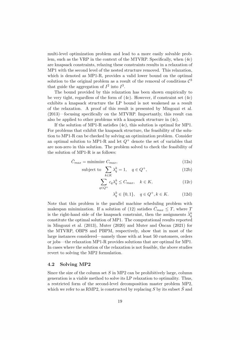
If the solution of MP1-R satisfies (4c), this solution is optimal for MP1.For problems that exhibit the knapsack structure, the feasibility of the solu-tion to MP1-R can be checked by solving an optimization problem. Consideran optimal solution to MP1-R and let Q+ denote the set of variables thatare non-zero in this solution. The problem solved to check the feasibility ofthe solution of MP1-R is as follows:
Cmax = minimize Cmax, (12a)
subject to∑k∈K
λkq = 1, q ∈ Q+, (12b)∑q∈Q+
cqλkq ≤ Cmax, k ∈ K, (12c)
λkq ∈ {0, 1}, q ∈ Q+, k ∈ K. (12d)
Note that this problem is the parallel machine scheduling problem withmakespan minimization. If a solution of (12) satisfies Cmax ≤ T , where Tis the right-hand side of the knapsack constraint, then the assignments λkqconstitute the optimal solution of MP1. The computational results reportedin Mingozzi et al. (2013), Muter (2020) and Muter and Oncan (2021) forthe MTVRP, OBPS and PBPM, respectively, show that in most of thelarge instances considered—namely those with at least 50 customers, ordersor jobs—the relaxation MP1-R provides solutions that are optimal for MP1.In cases where the solution of the relaxation is not feasible, the above studiesrevert to solving the MP2 formulation.
4.2 Solving MP2
Since the size of the column set S in MP2 can be prohibitively large, columngeneration is a viable method to solve its LP relaxation to optimality. Thus,a restricted form of the second-level decomposition master problem MP2,which we refer to as RMP2, is constructed by replacing S by its subset S and
19
relaxing the integrality constraints (5d). Letting π ≥ 0 and ζ ∈ R denotethe dual variables associated with constraints (5b) and (5c), respectively,the pricing subproblem of the second-level master problem (PSP2) is
mins∈S
cs − πas − ζ. (13)
Many of the details regarding column generation approaches for MP2are hidden in the definition of the set S. Since this set corresponds to I3,the solution approach for PSP2 must take into account the nested structureand the constraints that define the aggregation in levels 2 and 3. We willpresent three methods to solve this PSP2: branch-and-price, the two-phaseapproach, and the one-level method.
4.2.1 Branch-and-Price.
The PSP2 given in (13) can also be written as
(PSP2) minimize∑q∈Q
(cq−πaq)λq − ζ, (14a)
subject to∑q∈Q
eqλq ≤ f, (14b)
λq ∈ {0, 1}, q ∈ Q, (14c)
where the substitutions∑
q∈Q cqλsq = cs and
∑q∈Q aqλ
sq = as performed
in the second-level decomposition have been reversed. Constraints (14b)and (14c) induce the integer points corresponding to the solution set S. Inthe formulation of MP2, the PSP2 contains the constraints that define theaggregation of I2 into I3. As a result, the set Q is maintained in PSP2.
The large cardinality of Q can make the explicit enumeration of this setcumbersome. However, for small to medium sized instances problem struc-ture may facilitate the enumeration of this set. For example, Azi et al. (2010)show for the MTVRPTW that the route duration limit and time windowsmakes route enumeration possible. This pre-enumeration enables branch-and-price to be performed only on one-level. In the algorithm presented byAzi et al. (2010), each node in the graph for PSP2 denotes a pre-enumeratedfeasible route. This algorithmic structure conveniently eliminates the needto employ branch-and-price when solving PSP2. For the MTVRP, Mingozziet al. (2013) develop a bounding procedure based upon MP1-R to enumeratea subset of routes in Q that are necessary in the solution of MP2. Usingthese routes, the authors then perform an additional enumeration step togenerate the set of schedules in MP2 before solving it by an off-the-shelfsolver. In the context of staff rostering, Dohn and Mason (2013) presentan MP2 formulation that can be solved to integer optimality by only em-ploying a one-level branching scheme. The subproblem PSP2, while also
20

solved by column generation, doesn’t require branching to find integer opti-mal solutions. This is the result of formulating PSP2 such that all optimalsolutions to the LP relaxation satisfy the integrality requirements. A col-umn generator described by Mason and Smith (1998) is used to effectivelysolve PSP2.
When enumeration is not possible, column generation can be applied tosolve PSP2. If the optimal solutions to the LP relaxation of PSP2 do notsatisfy the integrality requirements, then branch-and-price is required. Thisleads to a nested column generation algorithm and the branching schemesare described as two-level branching. Letting θ ≤ 0 be the vector of dualvariables associated with (14b), the restricted pricing subproblem of thePSP2, denoted by PSP1, is given by
minq∈Q
cq − πaq − θeq. (15)
Since Q results from the first-level decomposition, we obtain the followingformulation by reversing the substitutions given in (3):
minimize (c−πA− θE)x, (16a)
subject to Bx ≥ d, (16b)
x ∈ Z+. (16c)
Example 4.1 PSP2 for the MTVRP can be written as
minimize∑q∈Q
cqλq − ζ, (17a)
subject to∑q∈Q
cqλq ≤ T, (17b)
∑q∈Q
aiqλq ≤ 1, i ∈ I1, (17c)
λq ∈ {0, 1}, q ∈ Q. (17d)
The above problem is a set-packing problem with a knapsack constraint. Thisform of subproblem also arises as PSP2 in other applications, such as OBPSand PBPM. An alternative form of this subproblem is a knapsack problemwith conflicts. The conflicts can be defined between pairs of members of Q,(qr, qp) : qr, qp ∈ Q, for which ∃i ∈ I1 : aiqr = aiqp = 1 (Bettinelli et al.(2017)). However, regardless of the formulation, PSP2 for the MTVRPtends to be a difficult problem to solve—even for moderately-sized instances.
Letting θ1 ∈ R− and θ2 ∈ R|J |− be the dual variables associated withconstraints (17b) and (17c), respectively, PSP1 is
minq∈Q
cq −∑i∈I1
πiaiq −∑i∈I1
θ2i aiq − θ1cq.
21

The routes in Q are characterized by elementarity and resource constraintsso that PSP1 manifests itself as the elementary shortest path problem withresource constraints (ESPPRC).
For the MP2 formulation of the MSCS problem in (11), PSP2 can bedefined as
maximize∑q∈Q
cqλq − 1, (18a)
subject to∑q∈Q
cqλq ≤ T, (18b)
λq ∈ Z+, q ∈ Q, (18c)
where T for this problem denotes the width of the stock roll, cq =∑
i∈I1 aiqciand cq =
∑i∈I1 aiqπi are the total width and reduced cost of the finished roll
pattern q ∈ Q, respectively. PSP2 is an unbounded knapsack problem whosevariables are not known explicitly unless Q is enumerated.
Letting θ denote the dual variable associated with (18b), PSP1 can bemodeled as the following unbounded knapsack problem:
maximize∑i∈I1
πiai − θ, (19a)
subject to tmin ≤∑i∈I1
ciai ≤ tmax, (19b)
ai ∈ Z+, i ∈ I1. (19c)
In regards to the MSCS, nested column generation has been employedin many studies tackling nested structures (Vanderbeck 2001, Song 2009,Muter and Sezer 2018). Song (2009) present various approaches to solvePSP2, which are based on a set partitioning heuristic. Vanderbeck (2001)enumerates the set I2 that is used in PSP1 to generate I3 dynamically byapplying column generation in the first level. The generation of cutting pat-terns I4 in PSP2 is achieved using a branch-and-bound algorithm where thelower bounds are obtained by Lagrangian relaxation and the upper boundsare found by executing a greedy heuristic.
In Muter and Sezer (2018), the application of branch-and-price to (18),which generates intermediate roll cutting patterns, is hindered by a well-known phenomenon of dichotomous branching in the cutting stock problems.The authors address this issue using a modification of the lexicographicalgorithm (Gilmore and Gomory 1963) to solve PSP2 to optimality. Atthe termination of column generation for MP2, an off-the-shelf solver isthen used to solve RMP2 as a MIP to produce an upper bound—in manyinstances this bound corresponds to the optimal solution.
There have been many applications of nested column generation to solvevariants of the VRP. Tilk et al. (2019) apply a nested column generation
22
algorithm to solve the MP2 formulation of the VRP with multiple resourceinterdependencies. Since PSP2 is formed of a large set of paths, columngeneration is applied to solve PSP1, which is formulated as an ESPPRC.Two types of branching schemes are used by Tilk et al. (2019) to solve PSP2.The first is based on the original variables and the second is a constraint-based branching. In a similar manner, branch-and-price is employed in bothlevels by Hennig et al. (2012) to solve the maritime scheduling problem. Inthe algorithm presented by Hennig et al. (2012), a constraint branchingscheme and heuristic pricing are employed.
For the PTVRP, Karabuk (2009) propose a nested column generationalgorithm in which the PSP2 generates routes that are formed of a set ofmini-clusters. The network underlying PSP2 specifies the nodes to repre-sent requests and the arcs correspond to mini-clusters. For the mini-clustergeneration in PSP1, the author presents a dynamic programming algorithmsimilar to that proposed in Ioachim et al. (1995). Since PSP2 exhibits thetotal unimodularity property, only one-level branchings are required to solvethe PTVRP presented by Karabuk (2009).
4.2.2 Two-phase Approach.
Solving PSP2 by branch-and-price can be both burdensome in terms of theeffort invested in coding and unstable in terms of performance. On the otherhand, the pre-enumeration of Q and solving PSP2 at every iteration of thecolumn generation algorithm is not always a viable option due to the size ofthis set. Rather than explicit enumeration, the column set can be implicitlyenumerated using dominance relations that are derived from the constraintsof PSP2, namely Eλ ≤ f . The implicit enumeration that generates thecolumns needed in the solution of PSP2 is called the first phase of the two-phase approach. After the non-dominated columns are generated, PSP2 issolved directly as an integer program in the second phase. The followingpropositions specify the general characteristics of the columns generated inthe first phase that are used in the second phase.
Proposition 4.1 For two variables λq, λq′ ∈ Z+, λq′ = 0 in all optimalsolutions if eq ≤ eq′ and cq − πaq ≤ cq′ − πaq′.
Proposition 4.2 For two variables λq, λq′ ∈ {0, 1}, λq = 0 in all optimalsolutions if eq ≤ eq′, cq−πaq ≤ cq′−πaq′ and there exists a row k in E suchthat ekq + ekq′ > fk.
Proposition 4.3 A column λq can exist in the solution of PSP2 if andonly if cq − πaq < 0.
Since the values of the dual variables π change at every solution of RMP2,the enumeration taking place in the first phase must be executed at every
23
call of PSP2, which would result in a distinct set of columns denoted byQ′ = {q ∈ Q : cq − πaq < 0}.
An example of the complete enumeration of Q at the outset of the columngeneration algorithm to solve MP2 is presented by Azi et al. (2010). Thispre-enumeration of Q can inflict a computational burden on the secondphase where each route in Q corresponds to a node in the shortest pathproblem with resource constraints on a route graph. The approach of Aziet al. (2010) can be enhanced by reducing Q to Q′ = {q ∈ Q : cq − πaq < 0}in the first phase by making use of the dual variables π so that the secondphase is applied to a smaller set at each iteration of the column generationalgorithm.
The two-phase approach has also been employed in Akca (2010) andMuter et al. (2014). This approach, which involves the enumeration of Q′ ateach iteration of the column generation algorithm, potentially causes scala-bility issues in PSP2 when the cardinality of Q′ is large. This is particularlyevident in the early iterations of the column generation algorithm—beforethe dual solutions have stabilized. Rather than enumerating Q′ at every it-eration, a heuristic enumeration scheme can be applied that generates onlya subset of Q′ to be utilized in the second phase to solve PSP2. The heuris-tic enumeration continues while a negative reduced cost column is found.Otherwise, exact enumeration is required. The exact enumeration of Q′ istypically only performed few times towards the end of the column generationalgorithm.
Two-phase approach has been applied to solve the MSCS (Muter andSezer (2018)) and its special version (Valerio de Carvalho and Rodrigues(1995)) in which each intermediate roll is cut into a single finished roll. ThePSP2 for this problem is the integer knapsack problem, which allows elimi-nation of many rolls I2 in the first level of this method due to Proposition4.1. Even though Valerio de Carvalho and Rodrigues (1995) pre-enumeratedthe set of intermediate rolls, the columns that don’t qualify for Q′ are nottaken into consideration in PSP2.
In some cases, the large cardinality of Q′ results from the set packingconstraints in PSP2 emerging in the form of (17c). For VRP extensions, theset packing constraints induce elementarity in the first level, which generatesa permutation of elements of I1. These constraints not only complicate theenumeration process in the first level but also proliferate the set Q′ thatforms the second level. Elementarity, i.e. each element of I1 can appear atmost once in each element of I2, is common across many applications. Onthe other hand, for the OBPS and PBPM, it is the combination, rather thanpermutation in the case of VRP extensions, of elements in I1 that coalescein the first phase of the two-phase approach to form Q′. For the OBPS andPBPM, Muter and Oncan (2021) and Muter (2020), respectively, addressthe adverse effect of the packing constraints by simply relaxing them. Theresulting problem is a 0-1 knapsack problem, which is easier to solve and
24

lends itself to a more efficient enumeration in the first phase. However, thesolution of the two-phase approach may contain some i ∈ I1 more thanonce and thus only provides a lower bound. In order to obtain the optimalsolution using this relaxation, Muter (2020) and Muter and Oncan (2021)employ a technique based on the enumeration of variables.
4.2.3 One-level Method.
The one-level method solves PSP2, given in (13), directly by generatingthe columns in S without a separate procedure for the generation of Q.In this approach, the MP2 results from a one-level decomposition definingI2′—rather than performing the steps of a two-level decomposition sequen-tially. The mathematical model of (13) associated with this approach canbe written as follows:
minimize (c−πA)x− ζ,subject to Bx ≤ d,
Ex ≤ f,x ∈ {0, 1}n+.
Despite its modularity, this model is challenging to solve. For the MTVRP,this approach entails a model that contains all constraints of (7a)-(7g) exceptfor (7b). In the solution of the VRP extensions where this subproblemis modeled as the ESPPRC, incorporating the constraints associated withthe transition from I2 to I3 in the one-level method adds new resourcesassociated with the members of this set.
A one-level method to solve the subproblem of MP2 of ILRSP is proposedin Akca (2010). This solution method employs a modified form of the la-beling algorithm presented by Feillet et al. (2004), where replenishment arcsare utilized to allow the vehicles to continue their schedules after a routeends at a depot. This approach can be adapted for any VRP extensionthat has a two-level decomposable structure. Examples for the MDVRPIand MTVRPTW are presented by Muter et al. (2014) and Hernandez et al.(2016), respectively. The computational experiments by Akca (2010) andMuter et al. (2014) show that the two-phase approach typically outperformsthe one-level method.
Zak (2002) applies the one-level method to solve the MSCS heuristically.The author modifies (18) by replacing the total width cq and the reducedcost cq of q ∈ Q with cq =
∑i∈I1 aiqci and cq =
∑i∈I1 aiqπi, respectively.
The resulting problem is not only large-scale but also non-linear due tomultiplication of λq and aiq. In order to circumvent these difficulties, Zak(2002) limits the number of new finished roll cutting pattern to be addedto the problem in each column generation iteration to one. This restrictionenabled Zak (2002) to solve the MSCS heuristically as an extension of the
25
knapsack problem. A similar heuristic approach is adopted by Wang andTang (2010) to solve the PBPM in which only one new batch is allowed toreside in a machine schedule generated by the PSP2.
4.3 Solving MP1
Solving the first-level decomposition model MP1 directly is an alternativeto solving MP2. Compared to the solution algorithms for MP2, which arehindered by PSP2 needing to generate s ∈ S, it has the advantage of dealingwith column set Q in a single level. For example, generating routes in thesolution of MTVRP is easier than generating schedules. However, restrict-ing the decomposition to a single level misses the opportunity to exploitproperties such as an improved lower bound and a more compact formula-tion that are only available after the second-level decomposition is applied.Even though solving MP1 by column generation is more practical in termsof solving the subproblem, a number of other issues affect the effectivenessof the overall branch-and-price scheme. For instance, considering MP1 forthe MTVRP, given by (8), the LP relaxation bound is considerably loose. Infact, relaxing the knapsack constraints (8c) does not deteriorate this bound.Moreover, the assignment of routes to vehicles represented by variables λkqcauses difficulties in the branch-and-bound tree due to symmetry.
For the MTVRPTW with duration limit, Hernandez et al. (2014) andMacedo et al. (2011) propose MP1 formulations that rely on the pre-enumerationof the route set—as in Azi et al. (2010). Methodologies used in these studiesdeal with the selection of routes by incorporating the constraint set Ex ≤ fdirectly into MP1, rather than handling their assignment to vehicles. Her-nandez et al. (2016) consider the MTVRPTW without a limitation on routeduration, which proliferates the number of routes to be incorporated com-pletely by pre-enumeration. In their MP1 formulation, the Ex ≤ f con-straints emerge as the time-indexed constraints that limit the number ofroutes performed at any time period to the fleet size. Hernandez et al.(2016) also propose a one-level method for the solution of the MP2 formula-tion. The computational experiments show that the proposed methodologyaimed at solving MP1 outperforms the one-level method.
Crevier et al. (2007) formulate an MP1 model for the MDVRPI, wherethe set Q corresponds to the inter-depot routes and the constraints Ex ≤ fimpose the connectivity of inter-depot routes to form schedules. The authorssolve this model heuristically by first generating a pool of inter-depot routes.Keeping the pool size relatively small, they managed to solve MP1 by anoff-the-shelf solver in a reasonable amount of time.
26

4.4 Solving MP1-2
The structure of MP1-2 requires the use of specialized algorithms to ef-fectively solve the corresponding problems. The main difficulty that arisesfrom the application of Dantzig-Wolfe reformulation to form MP1-2 is thatthe constraint set is dependent on the column set. Since the size of thecolumn set is exponential in the problem input, this formulation also bearsa prohibitively large number of constraints. The proliferation of constraintshas led to the development of algorithms combining a delayed constraintgeneration algorithm with a delayed column generation algorithm.
4.4.1 Simultaneous Column-and-Row Generation.
Applying column generation to MP1-2 entails the generation of both S andQ in a single model. However, when Q is replaced by Q to form the RMP,constraints (6c) associated with Q\Q are absent from the model. Hence,the generation of a new q ∈ Q\Q adds a constraint in (6c). Problems thatmeet a set of conditions and are amenable for this method are referred to asthe problems with column-dependent rows (Muter et al. 2013), and MP1-2 falls into this problem class. Recall that algorithms developed for MP2generate q ∈ Q during the solution of PSP2, which produces s ∈ S, whilethose designed for MP1 only generate q ∈ Q. Since Q and S reside in thesame level in MP1-2, the design issue becomes whether S and Q can begenerated in separate subproblems at the same level. Regardless, the dualsassociated with (6c) must be taken into account in the subproblems thatgenerate columns and trigger new constraints.
Note that due to constraints (6c), generating a q ∈ Q\Q when there is nos ∈ S in the RMP with hqs > 0 results in a degenerate iteration, since λq isfixed to zero. Thus, it is algorithmically more accurate to generate variablesin Q in tandem with S in a single subproblem. Generating columns fromQ and S simultaneously in the same subproblem can be achieved usingthe approaches described above to solve MP2. Further, we can show thatthe reduced cost of column s ∈ S resulting from applying simultaneouscolumn-and-row generation is equal to that resulting from applying columngeneration to MP2, which also attests to the equivalence of the subproblemof MP1-2 and PSP2.
Proposition 4.4 The pricing subproblem of MP1-2 resulting from the si-multaneous column-and-row generation is equivalent to PSP2.
Proof 4.1 The proof is given in the Appendix A.
A motivation for solving MP1-2, which grows both in columns and rowsand still hinges upon the solution of PSP2, lies in the capability of gen-erating Q and S separately. For instance, in MSCS formulation given in
27
(10), the one-to-many relationship between J , the index set of (10c), andQ induces that many finished roll cutting patterns can be identified for asingle intermediate roll width. This is in contrast with the other applica-tions of MP1-2 where there is a one-to-one relationship. An example isthe model for PBPM presented by Wang and Tang (2010) that leads to asingle subproblem generating machine schedules. A separate λ−generatingsubproblem also brings about the benefit of warming up the dual variablesfrom their initial erratic state. This subproblem can be invoked as long asit generates a negative reduced cost λ variable, which is then followed byPSP2 to generate ys, s ∈ S\S. In Zak (2002) and Muter and Sezer (2018),the λ−generating subproblem is called for each j ∈ J to generate finishedroll patterns from the existing intermediate rolls.
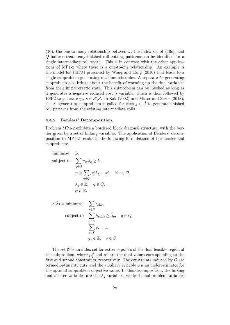
4.4.2 Benders’ Decomposition.
Problem MP1-2 exhibits a bordered block diagonal structure, with the bor-der given by a set of linking variables. The application of Benders’ decom-position to MP1-2 results in the following formulations of the master andsubproblem:
minimize ϕ,
subject to∑q∈Q
aiqλq ≥ b,
ϕ ≥∑q∈Q
µωq λq + ρω, ∀ω ∈ O,
λq ∈ Z, q ∈ Q,ϕ ∈ R.
z(λ) = minimize∑s∈S
csys,
subject to∑s∈S
hqsys ≥ λq, q ∈ Q,∑s∈S
ys = 1,
ys ∈ Z, s ∈ S.
The set O is an index set for extreme points of the dual feasible region ofthe subproblem, where µωq and ρω are the dual values corresponding to thefirst and second constraints, respectively. The constraints induced by O aretermed optimality cuts, and the auxiliary variable ϕ is an underestimator forthe optimal subproblem objective value. In this decomposition, the linkingand master variables are the λq variables, while the subproblem variables
28
are the ys variables. This is not the only decomposition achievable by ap-plying Benders’ decomposition. An equivalent decomposition can be foundby interchanging the master and subproblem variables, and correspondingconstraints.
The application of Dantzig-Wolfe reformulation and Benders’ decompo-sition to solve the MP1-2 formulation of the crew pairing and assignmentproblem is presented by Zeighami and Soumis (2019). In the formulationpresented by Zeighami and Soumis (2019), the assignment variables corre-spond to the y variables where the pairing variables correspond to the λvariables. The limitations of combining column generation and Benders’decomposition in this manner is addressed by Zeighami and Soumis (2019)through the formulation of weak Benders’ optimality cuts. It is reportedthat finding the optimal solution using the MP1-2 formulation is very dif-ficult, as such heuristic branching schemes are required. The experienceof Zeighami and Soumis (2019) demonstrate the challenges associated withapplying Benders’ decomposition to problems with column-dependent rows.These challenges are addressed in Muter et al. (2018) where a combined Ben-ders’ decomposition and simultaneous column-and-row generation algorithmis proposed.
4.4.3 Alternative algorithm.
Motivated by the solution approaches for the multi-stage cutting stock prob-lem, Gleixner et al. (2020) propose a column generation-based algorithm tosolve the recursive ring packing problem. A Dantzig-Wolfe reformulation isdeveloped to exploit one-level packings; thus, formulating the problem asMP1-2. The proposed formulation defines I1 as the set of rings, the set ofI2 contains the packings of circles (of equivalent diameter as the rings inI1) into rings and I3 is the set of packings of circles into rectangles. Thesolution approach begins with a partial enumeration of circular packings,partitioning all packings into feasible and unknown sets. Branch-and-priceis then performed to find feasible upper and lower bounds. If the boundingsolutions use any packings from the unknown set, then feasibility of thesepackings is checked. If the used unknown packings are found to be infeasible,constraints forbidding their use are imposed and the algorithm continues.
4.5 Implicit Enumeration
An alternative to branch-and-price for solving multi-level optimization prob-lems is predicated on a fundamental result of integer programming that cap-italizes on tight optimality gaps. The implicit enumeration approach uses areduced form of the master problem by enumerating a set columns that maypotentially reside in the optimal solution. The resulting master problem isthen solved by powerful off-the-shelf solvers. Baldacci and Mingozzi (2009)
29

has employed this approach in the solution of the VRP and its extensions.Consider the first- or second-level master problem, namely MP1 or MP2
respectively. Applying column generation to the LP relaxation provides alower bound on the optimal objective value of the respective master problem,which is denoted by zk where k = 1, 2 indicates the level of the masterproblem being tackled. When column generation terminates for the kth-level model, it also outputs dual feasible solutions for this model. Sinceupper bounding methods are out of the scope of this paper, we assumethat an upper bound z is at our disposal. The following proposition that isdefined for a given level k strips the immaterial variables out from the kth
level model when constructing the reduced form of the master problem.
Proposition 4.5 The columns whose reduced cost is larger than z−zk canbe discarded in the solution of MPk, k = 1, 2.
Let Q∗ and S∗ refer to the sets of columns in the reduced form of MP1and MP2, respectively. The enumeration of one of these sets is carriedout after the bounds of the respective model are obtained. The drawbacksof employing MP1 in an implicit enumeration scheme have already beenaddressed in the previous section. One significant drawback is the poorquality of the LP relaxation bound. On the other hand, the enumeration ofQ∗ is intrinsically simpler than that of S∗, since the former is handled in asingle step from I1 to I2 while the latter involves a further step from I2 toI3. Therefore, if MP2 and one of the methods designed for its solution isselected, a tight lower bound ensues at the expense of a more burdensomeenumeration. In several studies on multi-level problems (Mingozzi et al.2013, Muter 2020, Muter and Oncan 2021), MP2 has been adopted to reapthe benefits of tighter lower bounds; however, the set Q∗ is enumerated toform the reduced MP1. The gap between this lower bound z2 and a givenupper bound z sets a limit on the reduced costs in the enumeration of Q∗
due to the proposition given below.
Proposition 4.6 Let π and ζ denote the dual values outputted at the ter-mination of column generation applied to MP2. In the optimal solution ofMP1, a column q′ satisfying cq′ = cq′ − πaq′ > z − z2 is never selected.
Proof 4.2 The proof is given in the Appendix B.
As alluded to above, Q∗ is easier to enumerate than S∗ and its cardinalityis also considerably smaller. However, we remark that the application ofthis methodology in the literature has shown that the solution of MP1 issubstantially more difficult than MP2, which boasts a compactness that isachieved through the second-level decomposition.
Since PSP2 is itself an integer programming problem, implicit enumer-ation has implications on this problem as well. These implications are two-fold. First, in regards to the two-phase approach for solving PSP2, an
30

implicit enumeration procedure is required to identify the set of negativereduced cost columns Q′. For PSP2, a readily available upper bound iszero as this is the reduced cost of a basic variable of RMP2. If a fast lowerbounding method can be developed, which provides a lower bound zLB andduals θ of PSP2, all columns q ∈ Q′ that violate cq − πaq − θeq ≤ 0 − zLBcan be eliminated. This methodology to reduce the size of Q′, which formsthe reduced PSP2 in the second phase, has been applied by Muter et al.(2014) and Muter and Sezer (2018) in solving PSP2 of the MDVRPI andMSCS, respectively. In the latter work, a knapsack bound and duals wereused, while in the former work, a more complex LP relaxation bound is ob-tained. Second, implicit enumeration is an alternative to solving PSP2 bybranch-and-price. Rather than resorting to a branch-and-bound tree searchafter PSP2 is solved by column generation, one can make use of the lowerbound zCG alongside the duals π and θ and the trivial upper bound of zeroin the enumeration of q ∈ Q′ satisfying cq − πaq − θeq ≤ 0− zCG.
5 Final Remarks and Conclusion
This paper provides an overview of nested multi-level optimization problems.This overview covers the various formulations resulting from the applicationof decomposition techniques, a discussion of applications that have beenexamined in the literature and a presentation of state-of-the-art solutionmethods. As a summary, the main points and contributions of this paperare:
• Three alternative models based on Dantzig-Wolfe reformulation arepresented and their computational effectiveness with respect to ap-plications from the literature has been discussed. It is observed thatmost of the literature on nested decomposition tackle the MP2 formu-lations. Branch-and-price is the prevalent method for the solution ofPSP2.
• The constraints C2 and C3 are important determinants in the selectionof algorithms to solve MP2. If q ∈ Q and s ∈ S are allowed to containmultiple occurrences of an element of I1, the resulting subproblemsin both levels are exempt from the complicating elementarity require-ment. Furthermore, if I2 and I3 are formed of combinations, ratherthan permutations, of I1 and I2, respectively, the respective subprob-lems can generally be formulated on topologically sorted networks thatlimit the solution space considerably. These structures favor enumera-tive algorithms, such as the two-phase approach, which avoid the needto apply branch-and-price in the solution of PSP2.
• Unlike branch-and-price and the two-phase approach, the one-levelmethod solves MP2 by generating S directly through I2′ , which in-
31
volves both C2(x) and C3(x). In the examined applications, this ap-proach incorporates constraints associated with the third level C3(x)into PSP1, which is typically solved by dynamic programming. Thisbrings about an explosion in the state space, leading to the one-levelmethod being outperformed by the other methods that have been dis-cussed.
• The relaxation of constraints in MP1 leads to well-studied problemsin the literature. Depending on the relaxed constraint, the result-ing lower bound of MP1 can be very strong for instances with large|I1|. Moreover, one can capitalize on the available algorithms to solveMP1, which involve aggregation of elements only from I1 to Q, if itsformulation encapsulates the formation of S from Q effectively.
• Tackling MP1-2 gives rise to simultaneous column-and-row generation,which triggers generation of constraints along with columns. We showthat the subproblems of MP2 and MP1-2 are similar so that the algo-rithms presented for MP2 are still required for the solution of MP1-2.Furthermore, MP1-2 may be preferable over MP2 only if a one-to-many relation exists between the linking constraints and the variableset Q.
• Implicit enumeration of columns is an effective solution technique thathas been employed in several applications to find integer optimal so-lutions. Finding tight upper and lower bounds is of paramount im-portance for the success of this method. We show that the levels inwhich enumeration and column generation take place can be differentand should be chosen according to the simplicity of the algorithm inthe respective level.
This paper has shown that common multi-level structures are routinelyencountered in various application domains. Using the theoretical frame-work and generalized model formulations, we have shown that the mosteffective solution techniques are broadly applicable to solve numerous ap-plied optimization problems. With the increasing prevalence of genericbranch-cut-and-price solvers, such as Coluna (Coluna 2021), DIP (Galatiet al. 2012), and GCG (Bergner et al. 2015) the generalization of solutionapproaches will drive the development of software for the deployment ofstate-of-the-art column generation algorithms. Future work will involve theintegration of the key results from this paper into generic branch-cut-and-price solvers to support the formulation and solution of nested multi-leveloptimization problems.
32
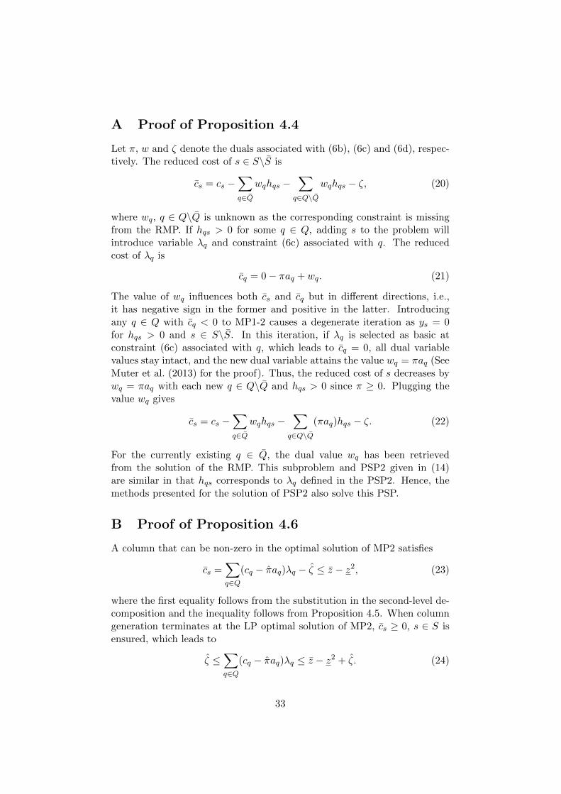
A Proof of Proposition 4.4
Let π, w and ζ denote the duals associated with (6b), (6c) and (6d), respec-tively. The reduced cost of s ∈ S\S is
cs = cs −∑q∈Q
wqhqs −∑
q∈Q\Q
wqhqs − ζ, (20)
where wq, q ∈ Q\Q is unknown as the corresponding constraint is missingfrom the RMP. If hqs > 0 for some q ∈ Q, adding s to the problem willintroduce variable λq and constraint (6c) associated with q. The reducedcost of λq is
cq = 0− πaq + wq. (21)
The value of wq influences both cs and cq but in different directions, i.e.,it has negative sign in the former and positive in the latter. Introducingany q ∈ Q with cq < 0 to MP1-2 causes a degenerate iteration as ys = 0for hqs > 0 and s ∈ S\S. In this iteration, if λq is selected as basic atconstraint (6c) associated with q, which leads to cq = 0, all dual variablevalues stay intact, and the new dual variable attains the value wq = πaq (SeeMuter et al. (2013) for the proof). Thus, the reduced cost of s decreases bywq = πaq with each new q ∈ Q\Q and hqs > 0 since π ≥ 0. Plugging thevalue wq gives
cs = cs −∑q∈Q
wqhqs −∑
q∈Q\Q
(πaq)hqs − ζ. (22)
For the currently existing q ∈ Q, the dual value wq has been retrievedfrom the solution of the RMP. This subproblem and PSP2 given in (14)are similar in that hqs corresponds to λq defined in the PSP2. Hence, themethods presented for the solution of PSP2 also solve this PSP.
B Proof of Proposition 4.6
A column that can be non-zero in the optimal solution of MP2 satisfies
cs =∑q∈Q
(cq − πaq)λq − ζ ≤ z − z2, (23)
where the first equality follows from the substitution in the second-level de-composition and the inequality follows from Proposition 4.5. When columngeneration terminates at the LP optimal solution of MP2, cs ≥ 0, s ∈ S isensured, which leads to
ζ ≤∑q∈Q
(cq − πaq)λq ≤ z − z2 + ζ. (24)
33
Due to (6c), if λq′ = 1 for some q′ ∈ Q, it should reside in one s ∈ S.Suppose that q′ satisfies (cq′ − πaq) > z − z2. Any s ∈ S containing q′
satisfies (23), i.e., cs ≤ z − z2, if the following condition holds:∑q∈Q\q′
(cq − πaq)λq < ζ,
This is not possible at the LP optimal solution of MP2, otherwise, thoseq ∈ Q\q′ with λq = 1 would form a schedule s′ with a negative reduced costcs′ < 0 due to the first inequality in (24). Therefore, a column q is in Q∗
only if cq − πaq ≤ z − z2.
References
Akca, Z. (2010). Integrated Location, Routing and Scheduling Problems: Modelsand Algorithms. PhD thesis, Lehigh University.
Azi, N., Gendreau, M., and Potvin, J.-Y. (2010). An exact algorithm for a vehiclerouting problem with time windows and multiple use of vehicles. EuropeanJournal of Operational Research, 202(3):756–763.
Baldacci, R. and Mingozzi, A. (2009). A unified exact method for solving differentclasses of vehicle routing problems. Mathematical Programming, 120:347–380.
Bard, J. F., Huang, L., Dror, M., and Jaillet, P. (1998). A branch and cut algorithmfor the VRP with satellite facilities. IIE Transactions, 30:821–834.
Bergner, M., Caprara, A., Ceselli, A., Furini, F., Lubbecke, M., Malaguti, E., andTraversi, E. (2015). Automatic Dantzig-Wolfe reformulation of mixed integerprograms. Mathematical Programming, 149(1–2):391–424.
Bettinelli, A., Cacchiani, V., and Malaguti, E. (2017). A branch-and-bound algo-rithm for the knapsack problem with conflict graph. INFORMS Journal onComputing, 29(3):457–473.
Coluna (2021). Coluna.jl. See https://github.com/atoptima/Coluna.jl. Lastaccessed: 11-10-2021.
Crevier, B., Cordeau, J.-F., and Laporte, G. (2007). The multi-depot vehicle rout-ing problem with inter-depot routes. European Journal of Operational Re-search, 176(2):756–773.
Desaulniers, G., Desrosiers, J., Dumas, Y., Marc, S., Rioux, B., Solomon, M.,and Soumis, F. (1997). Crew pairing at Air France. European Journal ofOperational Research, 97(2):245–259.
Desaulniers, G., Desrosiers, J., and Solomon, M., editors (2005). Column Genera-tion, New York. Springer.
Desaulniers, G., Errico, F., Irnich, S., and Schneider, M. (2016). Exact algorithmsfor electric vehicle-routing problems with time windows. Operations Research,64(6):1388–1405.
Dohn, A. and Mason, A. (2013). Branch-and-price for staff rostering: An efficientimplementation using generic programming and nested column generation.European Journal of Operational Research, 230(1):157–169.
34

Feillet, D., Dejax, P., Gendreau, M., and Gueguen, C. (2004). An exact algorithmfor the elementary shortest path problem with resource constraints: Applica-tion to some vehicle routing problems. Networks, 44:216–229.
Galati, M., Ralphs, T., and Wang, J. (2012). Computational experience withgeneric decomposition using the DIP framework. In Proceedings of RAMP2012.
Gilmore, P. C. and Gomory, R. E. (1963). A linear programming approach to thecutting-stock problem—Part II. Operations Research, 11(6):863–888.
Gleixner, A., Maher, S., Muller, B., and Pedroso, J. P. (2020). Price-and-verify: Anew algorithm for recursive circle packing using Dantzig-Wolfe decomposition.Annals of Operations Research, 284:527–555.
Hennig, F., Nygreen, B., and Lubbecke, M. E. (2012). Nested column generationapplied to the crude oil tanker routing and scheduling problem with splitpickup and split delivery. Naval Research Logistics, 59(3-4):298–310.
Hernandez, F., Feillet, D., Giroudeau, R., and Naud, O. (2014). A new exactalgorithm to solve the multi-trip vehicle routing problem with time windowsand limited duration. 4OR, 12(3):235–259.
Hernandez, F., Feillet, D., Giroudeau, R., and Naud, O. (2016). Branch-and-pricealgorithms for the solution of the multi-trip vehicle routing problem with timewindows. European Journal of Operational Research, 249(2):551–559.
Ioachim, I., Desrosiers, J., Dumas, Y., Solomon, M., and Villeneuve, D. (1995).A request clustering algorithm for door-to-door handicapped transportation.Transportation Science, 29(1):63–78.
Karabuk, S. (2009). A nested decomposition approach for solving the paratransitvehicle scheduling problem. Transportation Research Part B, 43(4):448–465.
Lubbecke, M. and Desrosiers, J. (2005). Selected topics in column generation.Operations Research, 53(6):1007–1023.
Macedo, R., Alves, C., Clautiaux, F., and Hanafi, S. (2011). Solving the ve-hicle routing problem with time windows and multiple routes exactly us-ing a pseudo-polynomial model. European Journal of Operational Research,214(3):536–545.
Maher, S. J. (2016). Solving the integrated airline recovery problem using column-and-row generation. Transportation Science, 50(1):216–239.
Mason, A. J. and Smith, M. C. (1998). A nested column generator for solvingrostering problems with integer programming. In International conference onoptimisation: techniques and applications, pages 827–834. Curtin Universityof Technology Perth, Australia.
Mingozzi, A., Roberti, R., and Toth, P. (2013). An exact algorithm for the multi-trip vehicle routing problem. INFORMS Journal on Computing, 25(2):193–207.
Muter, I. (2020). Exact algorithms to minimize makespan on single and paral-lel batch processing machines. European Journal of Operational Research,285(2):470–483.
Muter, I., Birbil, S. I., and Bulbul, K. (2013). Simultaneous column-and-row gen-eration for large-scale linear programs with column-dependent-rows. Mathe-matical Programming, 142(1-2):47–82.
35

Muter, I., Birbil, S. I., and Bulbul, K. (2018). Benders decomposition and column-and-row generation for solving large-scale linear programs with column-dependent-rows. European Journal of Operational Research, 264(1):29–45.
Muter, I., Cordeau, J.-F., and Laporte, G. (2014). A branch-and-price algorithm forthe multidepot vehicle routing problem with interdepot routes. TransportationScience, 48(3):425–441.
Muter, I. and Oncan, T. (2021). Order batching and picker schedul-ing in warehouse order picking. IISE Transactions, Published Online,http://dx.doi.org/10.1080/24725854.2021.1925178.
Muter, I. and Sezer, Z. (2018). Algorithms for the one-dimensional two-stage cuttingstock problem. European Journal of Operational Research, 271(1):20–32.
Song, S. H. (2009). A nested column generation algorithm to the meta slab alloca-tion problem in the steel making industry. International Journal of ProductionResearch, 47(13):3625–3638.
Tilk, C., Drexl, M., and Irnich, S. (2019). Nested branch-and-price-and-cut forvehicle routing problems with multiple resource interdependencies. EuropeanJournal of Operational Research, 276(2):549–565.
Valerio de Carvalho, J. M. and Rodrigues, A. G. (1995). An LP-based approach toa two-stage cutting stock problem. European Journal of Operational Research,84(3):580–589.
Vance, P., Barnhart, C., Johnson, E., and Nemhauser, G. (1997). Airline crewscheduling: A new formulation and decomposition algorithm. OperationsResearch, 45(2):188–200.
Vanderbeck, F. (2000). On Dantzig-Wolfe decomposition in integer programmingand ways to perform branching in a branch-and-price algorithm. OperationsResearch, 48(1):111–128.
Vanderbeck, F. (2001). A nested decomposition approach to a three-stage, two-dimensional cutting-stock problem. Management Science, 47(6):864–879.
Wang, G. and Tang, L. (2010). A row-and-column generation method to a batchmachine scheduling problem. In Proceedings of the Ninth International Sympo-sium on Operations Research and Its Applications (ISORA10), pages 301–308,Chengdu-Jiuzhaigou, China.
Zak, E. (2002). Row and column generation technique for a multistage cuttingstock problem. Computers & Operations Research, 29(9):1143–1156.
Zeighami, V. and Soumis, F. (2019). Combining Benders’ decomposition and col-umn generation for integrated crew pairing and personalized crew assignmentproblems. Transportation Science, 53(5):1479–1499.
36