an overview of sea state conditions and air-sea …an overview of sea state conditions and air-sea...

An overview of sea state conditions and air-sea fluxesduring RaDyO

Christopher J. Zappa,1 Michael L. Banner,2 Howard Schultz,3 Johannes R. Gemmrich,4

Russel P. Morison,5 Deborah A. LeBel,1 and Tommy Dickey6

Received 31 May 2011; revised 18 February 2012; accepted 27 February 2012; published 5 May 2012.

[1] Refining radiative-transfer modeling capabilities for light transmission through the seasurface requires a more detailed prescription of the sea surface roughness beyond theprobability density function of the sea surface slope field. To meet this need, exciting newmeasurement methodologies now provide the opportunity to enhance present knowledge ofsea surface roughness, especially at the microscale. In this context, two intensive fieldexperiments using R/P Floating Instrument Platform were staged within the Office ofNaval Research’s Radiance in a Dynamic Ocean (RaDyO) field program in the SantaBarbara Channel and in the central Pacific Ocean south of Hawaii. As part of this program,our team gathered and analyzed a comprehensive suite of sea surface roughnessmeasurements designed to provide optimal coverage of fundamental optical distortionprocesses associated with the air-sea interface. This contribution describes the ensemble ofinstrumentation deployed. It provides a detailed documentation of the ambientenvironmental conditions that prevailed during the RaDyO field experiments. It alsohighlights exciting new sea surface roughness measurement capabilities that underpin anumber of the scientific advances resulting from the RaDyO program. For instance, a newpolarimetric imaging camera highlights the complex interplay of wind and surface currentsin shaping the roughness of the sea surface that suggests the traditional Cox-Munkframework is not sufficient. In addition, the breaking crest length spectral density derivedfrom visible and infrared imagery is shown to be modulated by the development of thewavefield (wave age) and alignment of wind and surface currents at the intermediate(dominant) scale of wave breaking.

Citation: Zappa, C. J., M. L. Banner, H. Schultz, J. R. Gemmrich, R. P. Morison, D. A. LeBel, and T. Dickey (2012), Anoverview of sea state conditions and air-sea fluxes during RaDyO, J. Geophys. Res., 117, C00H19, doi:10.1029/2011JC007336.

1. Introduction

[2] There is substantial complexity in the local wind-driven sea surface roughness microstructure, including verysteep nonlinear wavelets and breakers. Nonlinear interfacialroughness elements: sharp crested waves, breaking waves aswell as the active whitecap regions, passive foam, subsur-face bubbles and spray they produce, contribute substan-tially to the distortion of the optical transmission through the

air-sea interface. These common surface roughness featuresoccur on a wide range of length scales, from the dominantsea state down to capillary waves. Traditional descriptors ofsea surface roughness are scale-integrated statistical proper-ties, such as significant wave height, mean square slope[e.g., Cox and Munk, 1954a, 1954b] and breaking proba-bility [e.g., Holthuijsen and Herbers, 1986]. Wave breakingsignatures range from large whitecaps with their residualpassive foam, down to the centimeter-scale microscalebreakers that do not entrain air. These numerous and diverseaspects of wave breaking are described in greater detail inreview articles [e.g., Banner and Peregrine, 1993; Melville,1996].[3] Present state-of-the-art radiative transfer models [e.g.,

Kattawar and Adams, 1989; Mobley, 1994] (for a completeoverview, see T. Dickey et al. (Recent advances in thestudy of optical variability in the near-surface and upperocean, submitted to Journal of Geophysical Research,2012) compute light transmission between the air and waterside marine boundary layers. For light passing through theair-sea interface, these models rely heavily on the classicalCox and Munk [1954b, 1956] sea surface slope statistics,particularly the surface slope probability density function.

1Ocean and Climate Physics Division, Lamont-Doherty EarthObservatory, Columbia University, Palisades, New York, USA.

2School of Applied Mathematics, University of New South Wales,Sydney, New South Wales, Australia.

3Department of Computer Science, University of Massachusetts,Amherst, Massachusetts, USA.

4Physics and Astronomy, University of Victoria, Victoria, BritishColumbia, Canada.

5School of Mathematics and Statistics, University of New South Wales,Sydney, New South Wales, Australia.

6Department of Geography, Graduate Program in Marine Sciences,University of California, Santa Barbara, California, USA.

Copyright 2012 by the American Geophysical Union.0148-0227/12/2011JC007336

JOURNAL OF GEOPHYSICAL RESEARCH, VOL. 117, C00H19, doi:10.1029/2011JC007336, 2012

C00H19 1 of 23

http://dx.doi.org/10.1029/2011JC007336

The rationale is that this statistical description adequatelydescribes the ocean surface roughness. While this maysuffice at modest wind speeds, it may not be optimal forstronger winds when wave breaking effects such as foambecome more prevalent and modify the optical transmis-sion and reflectivity of the sea surface.[4] In this context, current knowledge of the sea surface

roughness is incomplete. Only very limited spectral char-acterizations of open ocean wave height, slope and curvaturehave been measured to provide scale resolution for thesegeometrical sea roughness parameters [e.g., Hara et al.,1998] and their modulational properties [e.g., Hara et al.,2003]. Recently, field measurements of whitecap crestlength spectral density [e.g., Gemmrich et al., 2008; Phillipset al., 2001] have been reported. These studies have beenrestricted to whitecapping gravity waves where the signatureof wave breaking is captured by the optical contrast providedby the entrained air at the breaking crest. However, micro-scale breaking waves, which do not entrain air, can alsoimpact the optical transmissivity of the ocean surface. Todate, microscale breaker crest length spectral density mea-surements have been limited to the single laboratory study ofJessup and Phadnis [2005].[5] In order to refine radiative transfer modeling capabil-

ities, a more comprehensive prescription is needed of the seasurface roughness beyond the probability density function ofthe slopes. Wave height and slope spectra, and possibly theassociated bispectrum which represents the wave non-linearities, should be included in the modeling. Higher-ordermoments such as the curvature also need to be considered.Wave nonlinearity and breaking are also potentially impor-tant in creating surface geometry distortion, as well asattenuation and scattering of the light field. Envisaging alocal lens equivalent of the surface topography indicatesintuitively that these additional characterizations need to beincluded, but they are largely unknown at present.[6] To address these goals, two intensive field experi-

ments from R/P Floating Instrument Platform (FLIP) werestaged in the Office of Naval Research’s (ONR’s) Radiancein a Dynamic Ocean (RaDyO) field program in the SantaBarbara Channel and in the central Pacific Ocean southof Hawaii (Dickey et al., submitted manuscript, 2012).Our measurements contribute key background sea stateand environmental data for the RaDyO program. Theyalso provide crucial wave height and wave slope valida-tion data for verifying the fine-scale roughness measure-ments from our newly developed polarimetric camera.This instrument delivered new results for the mean squareslope of the sea surface out to millimeter scales, asfunctions of, for instance, the time-varying wind speed/stress, underlying dominant sea state and ocean currents.In addition, our comprehensive video and infrared imag-ery provided concomitant statistical distributions of spec-tral density of whitecap crest length per unit area indifferent scale bands of propagation speed, and similarlyfor the microscale breakers.[7] Previous studies tend to show heavily averaged proper-

ties of sea state, mean squared slope and breaking distributions.To our knowledge, no published studies to date investigatetime-resolved variations with respect to the synoptic condi-tions. During RaDyO, the appreciable observation period andcapacity to gather large data sets of multiple synoptic fields

(i.e., atmospheric, ocean, wave) provides an interestingopportunity to explore in detail how these short wave rough-ness fields respond to synoptic variables.

2. Experiments, Study Sites, and Platforms:Observational Programs UndertakenDuring RaDyO

[8] Two experiments defined the RaDyO program. Thefirst field experiment was performed in the Santa BarbaraChannel (SBC) from 3 to 25 September 2008. This settingwas selected because it was expected to provide a relativelybenign wind-wave state regime and easy access to shoresince several new or prototype instrumentation systems werebeing utilized. The second RaDyO field experiment tookplace in the central Pacific Ocean south of Hawaii from24 August to 15 September 2009. This location was selectedbecause of its climatologically high, persistent wind speedsand sea states, its optically clear waters, and its open oceancharacter.[9] Both experiments during RaDyO utilized R/P FLIP

and the R/V Kilo Moana, a SWATH vessel. Both providestable platforms for studies of meteorology, air-sea interac-tion, and physical oceanography. For the Santa BarbaraChannel RaDyO experiment, R/P FLIP was moored in placeat 34.2053�N, 119.6288�W in water of depth 168 m using atwo-point mooring (Figure 1). Some tilting of the R/P FLIPdeveloped due to the currents and winds. In particular, R/PFLIP had a typical lean angle of 3–7� due to strong currentsand about 0–5� due to wind forcing. These conditions wereaccompanied by a measurable oscillation in R/P FLIP’sheading with an approximately 2 min period. Instrumentswere deployed from R/P FLIP’s booms to minimize theinfluence of flow distortion and superstructure interference.The R/V Kilo Moana departed from Port Hueneme on8 September 2008 and returned on 23 September 2008. Forreference, R/V Kilo Moana sampled on station about 2 kmnorth of R/P FLIP during the SBC experiment. For thecentral Pacific Ocean experiment south of Hawaii, R/P FLIPwas freely drifting at a speed of 36.5 � 8.2 cm s�1 to thewest as shown in Figure 2. This anticipated high sea stateexperiment was carried out in the specific region ofapproximately 17.5� to 18.0�N, 155.5� to 160.0�W, south ofthe Hawaiian islands from 22 August to 14 September. TheKilo Mona left Sand Island, HI on 22 August and returnedon 14 September. For most of this time it was in the desig-nated experiment area, but for 2 days moved into the lee ofthe large island, to get protection from tropical storm Hilda,and to perform some calm seas/low wind experiments. Dueto the passage of tropical storm Hilda, R/P FLIP’s departurefrom Pearl Harbor was delayed 5 days.

3. Measurement Systems

3.1. Instrument Deployment Overview

[10] Figure 3 shows the instrumentation deployed fromthe 20 m starboard boom on R/P FLIP during the field mea-surements in the Santa Barbara Channel and in the centralPacific Ocean south of Hawaii. An environmental moni-toring system was deployed from the end of the boom thatincluded a sonic anemometer, a water vapor sensor, a RH/T/

ZAPPA ET AL.: RADYO WAVES AND FLUXES C00H19C00H19

2 of 23

P probe, a motion package, a pyranometer, and a pyrge-ometer. Meteorological measurements included: near-sur-face barometric pressure, three-component wind velocity,relative and specific humidity, air temperature, longwavedownwelling radiative flux, and shortwave downwelling

irradiance. All sensors were mounted at nominally 10 mabove sea level.[11] Two orthogonal line scanning lidars, synchronized

for zero crosstalk were deployed in addition to two laseraltimeters. Two visible cameras were mounted at the end of

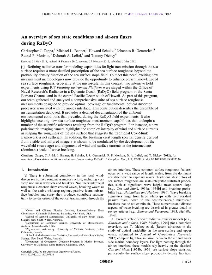
Figure 1. Mooring location of R/P FLIP (34.2053�N, 119.6288�W) using a two-point mooring in waterof depth 168 m during the Santa Barbara Channel experiment.

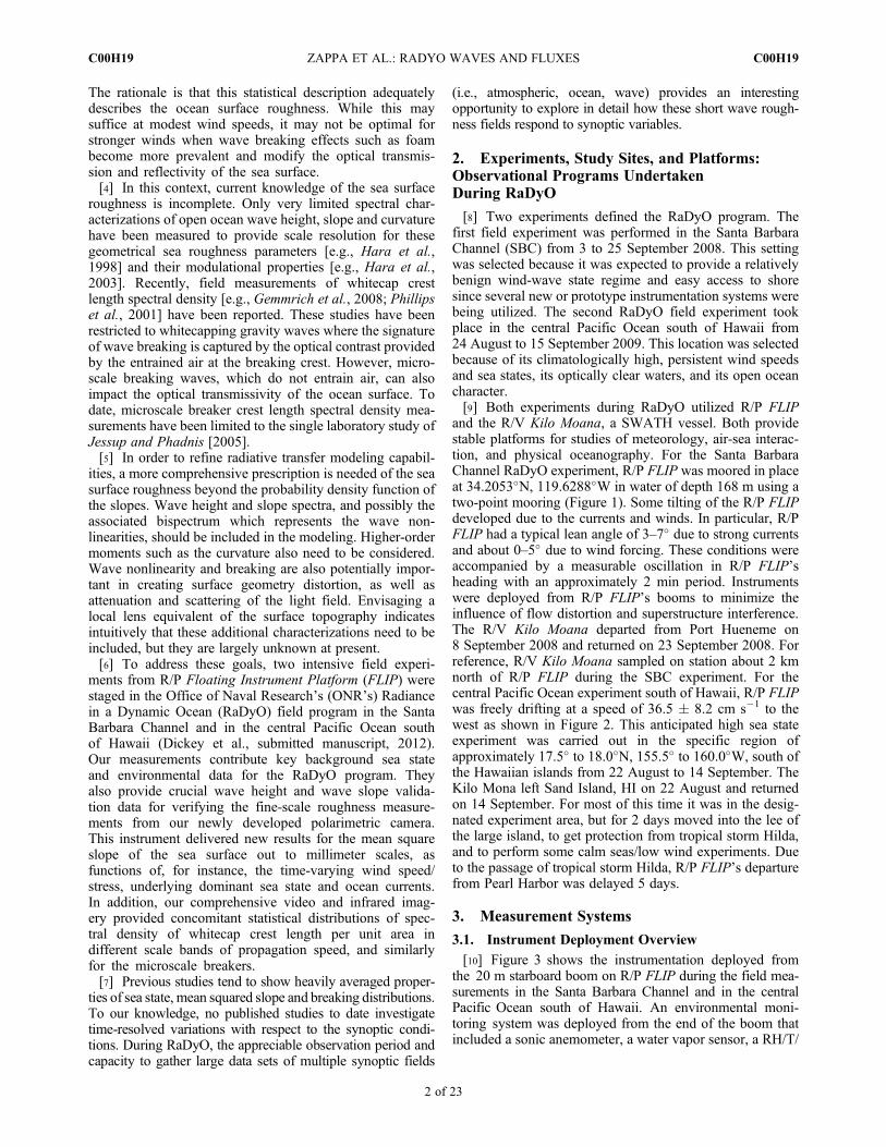
Figure 2. Drifting trajectory followed by R/P FLIP from 22 August to 14 September 2009 during theRaDyO experiment in the central Pacific Ocean south of Hawaii. The drift speed was 36.5 � 8.2 cm s�1

toward the west. R/P FLIP started at 17.6515�N, 156.5640�W and finished at 17.8218�N, 159.1984�W.


3 of 23

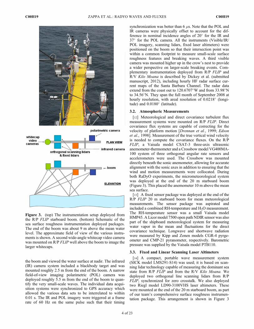
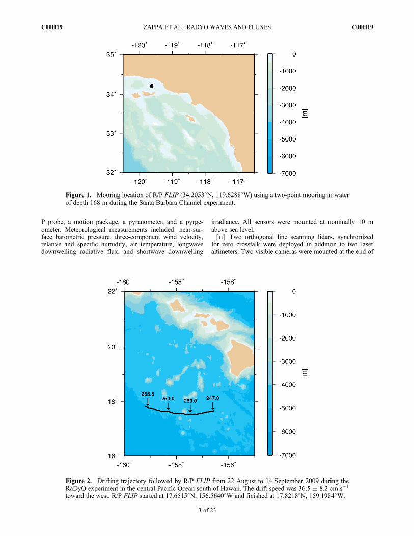
the boom and viewed the water surface at nadir. The infrared(IR) camera system included a blackbody target and wasmounted roughly 2.5 m from the end of the boom. A narrowfield-of-view imaging polarimetric (POL) camera wasdeployed roughly 5.5 m from the end of the boom to quan-tify the very small-scale waves. The individual data acqui-sition systems were synchronized to GPS accuracy whichallowed the various data sets to be interrelated to within0.01 s. The IR and POL imagery were triggered at a framerate of 60 Hz on the same pulse such that their timing

synchronization was better than 6 ms. Note that the POL andIR cameras were physically offset to account for the dif-ference in nominal incidence angles of 20� for the IR and37� for the POL camera. All the instruments (Visible/IR/POL imagery, scanning lidars, fixed laser altimeters) werepositioned on the boom so that their intersection point waswithin a common footprint to measure small-scale surfaceroughness features and breaking waves. A third visiblecamera was mounted higher up in the crow’s nest to providea wider perspective on larger-scale breaking events. Com-plementary instrumentation deployed from R/P FLIP andR/V Kilo Moana is described by Dickey et al. (submittedmanuscript, 2012), including hourly HF radar surface cur-rent maps of the Santa Barbara Channel. The radar dataextend from the coast out to 120.6707�W and from 33.98�Nto 34.56�N. They span the full month of September 2008 athourly resolution, with areal resolution of 0.0218� (longi-tude) and 0.0180� (latitude).

3.2. Atmospheric Measurements

[12] Meteorological and direct covariance turbulent fluxmeasurement systems were mounted on R/P FLIP. Directcovariance flux systems are capable of correcting for thevelocity of platform motion [Drennan et al., 1999; Edsonet al., 1998]. Measurement of the true vertical wind velocityis needed to compute the covariance fluxes. On the R/PFLIP, a Vaisala model CSAT-3 three-axis ultrasonicanemometer-thermometer and a Crossbowmodel VG400MA-100 system of three orthogonal angular rate sensors andaccelerometers were used. The Crossbow was mounteddirectly beneath the sonic anemometer, allowing for accuratealignment with the sonic axes in addition to ensuring that thewind and motion measurements were collocated. Duringboth RaDyO experiments, the micrometeorological systemwas deployed at the end of the 20 m starboard boom(Figure 3). This placed the anemometer 10 m above the meansea surface.[13] A fixed sensor package was deployed at the end of the

R/P FLIP 20 m starboard boom for mean meteorologicalmeasurements. The sensor package was aspirated andincluded a combined RH-temperature and H2O measurement.The RH-temperature sensor was a small Vaisala modelHMP45. A Licor model 7500 open path NDIR sensor was alsopart of the shipboard meteorological system for measuringwater vapor in the mean and fluctuations for the directcovariance technique. Longwave and shortwave radiationwere measured by Kipp and Zonen models CGR-4 pyrge-ometer and CMP-21 pyranometer, respectively. Barometricpressure was supplied by the Vaisala model PTB110.

3.3. Fixed and Linear Scanning Laser Altimeters

[14] A compact, portable wave measurement system(SICK model LMS291-S14) was used; it is based on scan-ning lidar technology capable of measuring the dominant seastate from R/P FLIP and from the R/V Kilo Moana. Wedeployed two orthogonal line scanning lidars from R/PFLIP, synchronized for zero crosstalk. We also deployedtwo Riegl model LD90-3100VHS laser altimeters. Thesewere mounted at the end of the 20 m starboard boom, as partof our team’s comprehensive surface roughness instrumen-tation package. This arrangement is shown in Figure 3

Figure 3. (top) The instrumentation setup deployed fromthe R/P FLIP starboard boom. (bottom) Schematic of thesea surface roughness instrumentation deployed packages.The end of the boom was about 9 m above the mean waterlevel. The approximate field of view of the various instru-ments is shown. A second wide-angle whitecap video camerawas mounted on R/P FLIP well above the boom to image thelarger whitecaps.


4 of 23

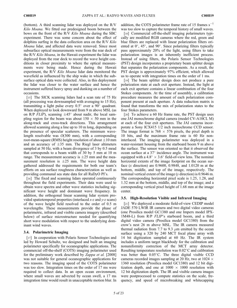
(bottom). A third scanning lidar was deployed on the R/VKilo Moana. We fitted our predesigned boom between thebows on the front of the R/V Kilo Moana during the SBCexperiment. There was some concern about the effect ofdolphins surfing in the data collection area on the R/V KiloMoana lidar, and affected data were removed. Since mostsubsurface optical measurements were from the rear deck ofthe R/V Kilo Moana, in the Hawaii experiment the lidar wasdeployed from the rear deck to record the wave height con-ditions in closer proximity to where the optical measure-ments were being made. Hence during the Hawaiiexperiment, the R/V Kilo Moana lidar data monitored thewavefield as influenced by the ship wake in which the sub-surface optical data were collected. Also, in this deploymentthe lidar was closer to the water surface and hence theinstrument suffered heavy spray and dunking on a number ofoccasions.[15] The SICK scanning lidars had a scan rate of 75 Hz

(all processing was downsampled with averaging to 15 Hz),transmitting a light pulse every 0.5� over a 90� quadrant.When deployed to look downward from 9 m above MSL (ason R/P FLIP), scanning �45� about nadir, the local sam-pling region for the beam was about 150 � 50 mm in thealong-track and cross-track directions. This arrangementallowed scanning along a line up to 10 m long, depending onthe presence of specular scatterers. The minimum wave-length resolvable was O(300 mm), with a correspondingroot-mean-square (RMS) height resolution of about�10 mmand an accuracy of �35 mm. The Riegl laser altimeterssampled at 50 Hz, with a beam divergence of 3 by 0.5 mradthat corresponds to a beam width of 30 by 5 mm at 10 mrange. The measurement accuracy is �25 mm and the mea-surement resolution is �25 mm. The wave height datagathered addressed the requirements for both our team’sefforts on sea surface roughness characterization as well asproviding communal sea state data for all RaDyO PI’s.[16] The fixed and scanning lidars operated continuously

throughout the field experiments. Their data were used toobtain wave spectra and other wave statistics including sig-nificant wave height and dominant wave frequency. Inaddition, the orthogonal linear scanning lidar system pro-vided spatiotemporal properties (interlaced x-z and y-z scans)of the wave height field resolved to the order of 0.5 mwavelengths. These measurements provide the phase ofpolarimetric, infrared and visible camera imagery (describedbelow) of surface microstructure needed for quantifyingshort wave modulation with respect to the underlying dom-inant wind waves.

3.4. Polarimetric Imaging

[17] In cooperation with Polaris Sensor Technologies andled by Howard Schultz, we designed and built an imagingpolarimeter specifically for oceanographic applications. Thecommercial off-the-shelf (COTS) imaging polarimeter usedfor the preliminary work described by Zappa et al. [2008]was not suitable for general oceanographic applications fortwo reasons. The imaging speed of the COTS polarimeterwas too slow. Integration times on the order of 17 ms wererequired to collect data. In an open ocean environment,where small waves are advected by ocean swell, a 17 msintegration time would result in unacceptable motion blur. In

addition, the COTS polarimeter frame rate of 15 frames s�1

was too slow to capture the temporal history of small waves.[18] Commercial off-the-shelf imaging polarimeters typi-

cally are modified RGB cameras where the red, green andblue filters are replaced with linear polarization filters ori-ented at 0�, 45�, and 90�. Since polarizing filters typicallypass approximately 20% of the light, using filters to takepolarization images is an inherently inefficient process.Instead of using filters, the Polaris Sensor Technologies(PST) design incorporates a proprietary beam splitter designthat separates the polarization components. As a result, thePST design is approximately 97% efficient, which allowedus to operate with integration times on the order of 1 ms.[19] The beam splitter design does not produce a pure

polarization state at each exit aperture. Instead, the light ateach exit aperture contains a linear combination of the fourStokes components. At the time of assembly, a calibrationprocedure measures the amount of each polarization com-ponent present at each aperture. A data reduction matrix isfound that transforms the mix of polarization states to thefour Stokes parameters.[20] To achieve a 60 Hz frame rate, the PST design uses

one JAI monochrome digital camera (model CV-A10CL M)at each of the four exit apertures. The JAI cameras incor-porate a Sony ICX415 1/2 inch monochrome CCD sensor.The image format is 768 � 576 pixels, the pixel depth is10 bits, and the maximum frame rate is 60 Hz non-interlaced. The imaging polarimeter was deployed in awater-resistant housing from the starboard boom 9 m abovethe surface. The sensor was oriented so that it observed theocean surface at a 37� incidence angle. The instrument wasequipped with a 4.8� � 3.6� field-of-view lens. The nominalhorizontal extents of the image footprint on the ocean sur-face (x direction) are 0.9600, 0.9848, and 1.0120 m at thebottom, middle, and top of the image, respectively. Thenominal vertical extent of the image (y direction) is 0.9646 m.The corresponding horizontal pixel scale is 1.25, 1.28, and1.32 mm at the bottom, middle, and top of the image; and acorresponding vertical pixel height of 1.68 mm at the imagecenter.

3.5. High-Resolution Visible and Infrared Imaging

[21] We deployed a moderate field-of-view CEDIP modelJADE 570 LWIR IR camera and two digital video cameras(one Prosilica model GC1380 and one Imperx model IPX-1M48-L) from R/P FLIP’s starboard boom, and a thirddigital video camera (Prosilica model GC1380) from thecrow’s nest 26 m above MSL. The IR camera measuredthermal radiation from 7.7 to 9.3 mm emitted by the oceansurface using a 320 by 240 MCT focal plane array with14 bit digitization sampled at 60 Hz. The IR systemincludes a uniform target blackbody for the calibration andnonuniformity correction of the MCT array detector.Resulting temperature resolution was 0.02�C and calibrationwas better than 0.05�C. The three digital visible CCDcameras recorded images sampling at 20 Hz, two at 1024 �1360 resolution (Prosilica model GC1380) and 12 bit digi-tization depth, and one at 1000 � 1000 resolution with12 bit digitization depth. The IR and visible camera imageswere postprocessed to compute statistics on the scale, fre-quency, and speed of microbreaking and whitecapping


5 of 23

events from scales of order 0.1 m s�1 up to scales of order10 m s�1. In particular, these data were used for determin-ing breaking crest length spectral density distributions andtheir higher moments.[22] The three cameras were used to observe wave

breaking, foam, and whitecapping over fields of 10 by 15 m(2 cameras) and 100 by 200 m (1 camera). The formercameras were mounted near the fixed and scanning lidarsystems close to the end of a boom (�9 m height) to measureintermediate scale breakers while the other was mounted onR/P FLIP’s crow’s nest at about 26 m above water level for abroader viewing angle to record larger scale breaking events.The sampling rates for all cameras were either 10 or 20 Hz.Data were generally collected for 20 min every hour duringdaylight hours; however, data were recorded more oftenduring periods of more frequent wave breaking events.Overall, 37 h over 13 days were recorded during the SBCexperiment and 21 h over 5 days were recorded during theexperiment south of Hawaii. The individual data acquisitionsystems were synchronized to GPS accuracy which allowedthe IR and visible imagery data sets to be interrelated towithin 0.01 s.

3.6. Ocean Skin Temperature Measurements

[23] A longwave narrow field-of-view Heitronics modelKT-15.82 LWIR radiometer (8–14 mm) was directed sky-ward to discriminate real from apparent ocean surface tem-perature variability during both field experiments from R/PFLIP. During the Santa Barbara Channel experiment, weused the skyward radiometer at 20� zenith angle in combi-nation with the JADE camera at 20� incidence angle todetermine the skin temperature. During the Hawaii experi-ment, we deployed a second Heitronics model KT-15.82radiometer that viewed the ocean surface at an incidenceangle of 25� with the skyward radiometer at 25� zenithangle. The combination of Heitronics skyward and down-ward looking radiometers provided a continuous time seriesof skin temperature, in addition to the random samples ofskin temperature made by the JADE camera. We use themethod outlined in equation (A2) of Appendix A of Zappaet al. [1998] to calculate the skin temperature.

4. Results and Discussion

4.1. Ambient Environmental Conditions

[24] The general wind pattern in Southern Californiaduring summer is determined by the position and strength ofthe subtropical anticyclone (i.e., surface high-pressure sys-tem) over the eastern North Pacific. In addition, a surfacethermal low-pressure system usually forms over the south-western U.S. in late summer or early autumn, and plays asignificant role in modifying horizontal pressure gradientsand wind regimes in central and southern California [e.g.,Dorman and Winant, 1995; Winant and Dorman, 1997].Many studies have extensively investigated the dynamics ofatmospheric circulations in the SBC during summertime[e.g.,Dorman and Winant, 1995, 2000;Dorman and Koračin,2008; Skyllingstad et al., 2001; Winant and Dorman, 1997].The typical summer day is marked by strong northwesterlywinds off the western coast of southern California. As thewinds turn at Point Conception (34.449�N, 120.471�W) and

enter the SBC, there is a significant increase in speeds from5 m s�1 over Point Conception to 10 m s�1 over the westernpart of the SBC [Skyllingstad et al., 2001]. Wind speedsthen decrease rapidly (�3 m s�1) over the eastern part ofSBC and winds turn westerly. Significant diurnal variationsexist in the atmospheric circulation and marine boundarylayer (MBL) associated with synoptic conditions, hydraulicflow, thermal effects, land-sea breeze circulations and seasurface temperature gradients in the channel [Skyllingstadet al., 2001].[25] The atmospheric conditions during the experiment

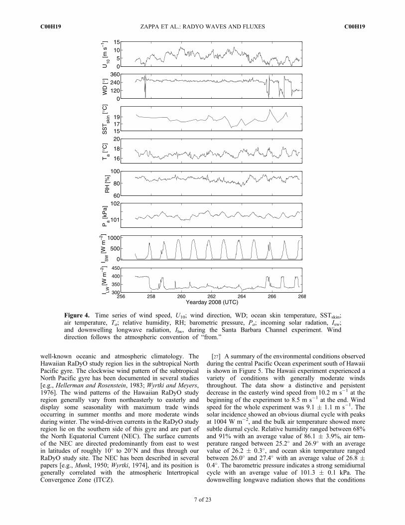
were important for the physical forcing in terms of waves,mixing, and currents as they all influence the temporal andspatial variability of the optical properties and the subsurfacelight fields. A summary of the environmental conditionsobserved during the Santa Barbara Channel study is shownin Figure 4. Throughout this paper all times are given asUTC, using the yearday definition: 1 January, noon = year-day 1.5. Mean surface winds were systematically from thenorthwest in the region near Point Conception with littlediurnal variation in direction and slight changes in intensity.In contrast, mean surface winds in the eastern SBC wereprimarily from the west with small variations in direction butwith considerable changes in intensity. The SBC experimentexperienced a variety of conditions with generally lowwinds in the early morning with mean wind speed of4.8 � 2.7 m s�1 (all plus/minus bounds refer to a combi-nation of natural variability and measurement uncertainty asexpressed by the standard deviation), and strong sea breezesup to 12 m s�1 in the evening with mean wind speeds of7.1 � 2.2 m s�1. The data show a distinctive and persis-tent diurnal structure to the wind speed that was strongerin the afternoon relative to the night and morning. Windspeed referenced to 10 m, U10, for the whole experimentwas 5.8 � 2.5 m s�1. The solar incidence, bulk air tem-perature, relative humidity, and ocean skin temperatureshow obvious diurnal cycles. The solar incidence showedpeaks of up to 861 W m�2. Relative humidity rangedbetween 75% and 94% with an average value of 86.5 �3.6%, air temperature ranged between 15.8� and 18.4� withan average value of 16.8 � 0.5�, and ocean skin tempera-ture ranged between 15.9� and 21.1� with an average valueof 18.3 � 1.0�. The barometric pressure indicates a semi-diurnal cycle with an average value of 101.2 � 0.1 kPa.The downwelling longwave radiation shows that the con-ditions were relatively clear (310–340 W m�2) for most ofthe experiment with periods of cloudiness (near 400 W m�2)that occurred predawn and in the early morning on days258 and 265–268. For the purposes of further discussion,the data is separated into three regimes: days 257–259,260–263, and 264–268. The wind speed for these threeregimes was 5.5 � 2.4, 7.6 � 1.8, and 4.1 � 2.1 m s�1,respectively. The diurnal cycles for bulk air temperature,relative humidity, and ocean skin temperature were stron-gest during the third regime and less intense earlier in theexperiment.[26] The location of the RaDyO experiment in the central

Pacific Ocean experiment south of Hawaii was selectedbecause of its climatologically high, persistent wind speeds,its well-developed wavefield with strongly forced sea states,its optically clear waters, and its open ocean character with a


6 of 23

well-known oceanic and atmospheric climatology. TheHawaiian RaDyO study region lies in the subtropical NorthPacific gyre. The clockwise wind pattern of the subtropicalNorth Pacific gyre has been documented in several studies[e.g., Hellerman and Rosenstein, 1983; Wyrtki and Meyers,1976]. The wind patterns of the Hawaiian RaDyO studyregion generally vary from northeasterly to easterly anddisplay some seasonality with maximum trade windsoccurring in summer months and more moderate windsduring winter. The wind-driven currents in the RaDyO studyregion lie on the southern side of this gyre and are part ofthe North Equatorial Current (NEC). The surface currentsof the NEC are directed predominantly from east to westin latitudes of roughly 10� to 20�N and thus through ourRaDyO study site. The NEC has been described in severalpapers [e.g., Munk, 1950; Wyrtki, 1974], and its position isgenerally correlated with the atmospheric IntertropicalConvergence Zone (ITCZ).

[27] A summary of the environmental conditions observedduring the central Pacific Ocean experiment south of Hawaiiis shown in Figure 5. The Hawaii experiment experienced avariety of conditions with generally moderate windsthroughout. The data show a distinctive and persistentdecrease in the easterly wind speed from 10.2 m s�1 at thebeginning of the experiment to 8.5 m s�1 at the end. Windspeed for the whole experiment was 9.1 � 1.1 m s�1. Thesolar incidence showed an obvious diurnal cycle with peaksat 1004 W m�2, and the bulk air temperature showed moresubtle diurnal cycle. Relative humidity ranged between 68%and 91% with an average value of 86.1 � 3.9%, air tem-perature ranged between 25.2� and 26.9� with an averagevalue of 26.2 � 0.3�, and ocean skin temperature rangedbetween 26.0� and 27.4� with an average value of 26.8 �0.4�. The barometric pressure indicates a strong semidiurnalcycle with an average value of 101.3 � 0.1 kPa. Thedownwelling longwave radiation shows that the conditions

Figure 4. Time series of wind speed, U10; wind direction, WD; ocean skin temperature, SSTskin;air temperature, Ta; relative humidity, RH; barometric pressure, Pa; incoming solar radation, Isw;and downwelling longwave radiation, Ilw, during the Santa Barbara Channel experiment. Winddirection follows the atmospheric convention of “from.”


7 of 23

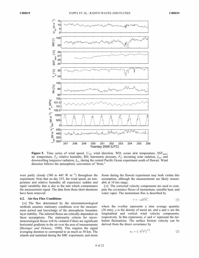
were partly cloudy (380 to 445 W m�2) throughout theexperiment. Note that on day 253, the wind speed, air tem-perature and relative humidity all experience sudden andrapid variability that is due to the rain which contaminatesthe measurement signal. The data from these short durationshave been removed.

4.2. Air-Sea Flux Conditions

[28] The flux determined by the micrometeorologicalmethods assumes stationary conditions over the measure-ment period and knowledge of the atmospheric boundarylayer stability. The inferred fluxes are critically dependent onthese assumptions. The stationarity criteria for micro-meteorological fluxes will be violated if there are significanthorizontal gradients in the air over the area of measurements[Businger and Delaney, 1990]. This requires the signalaveraging duration to correspond to as much as 50 km. Theislands and mainland during the SBC experiment, and storm

fronts during the Hawaii experiment may both violate thisassumption, although the measurements are likely reason-able at 10 km range.[29] The corrected velocity components are used to com-

pute the covariance fluxes of momentum, sensible heat, andwater vapor. The momentum flux is described by

t ¼ �ru′w′; ð1Þ

where the overbar represents a time average quantity(20 min), r is the density of moist air, and u and w are thelongitudinal and vertical wind velocity components,respectively. In this expression, u′ and w′ represent the tur-bulent fluctuations. The surface friction velocity can bederived from the direct covariance by

u� ¼ �u′w′� �1=2

: ð2Þ

Figure 5. Time series of wind speed, U10; wind direction, WD; ocean skin temperature, SSTskin;air temperature, Ta; relative humidity, RH; barometric pressure, Pa; incoming solar radation, Isw; anddownwelling longwave radiation, Ilw, during the central Pacific Ocean experiment south of Hawaii. Winddirection follows the atmospheric convention of “from.”


8 of 23

[30] The turbulent air-sea fluxes for sensible, Hs, andlatent, Hl, heat can also be measured using w′ with fluctu-ating temperature and water vapor concentrations, giving

Hs ¼ rcpw′ T ′ ð3Þ

and

Hl ¼ rLEw′ q′ ; ð4Þ

where cp is the specific heat for moist air, LE is the water latentheat of vaporization, T is the air temperature, and q is thespecific humidity. The CSAT3 sonic anemometer measurestemperature based on the speed of sound, which is a functionof density; hence the result must be corrected for water vapor.The sensible heat flux is determined following Dupuis et al.[1997] by w′T ′ ¼ w′T ′sonic � 0:518Tw′q′

� �= 1þ 0:518qð Þ ,

where Tsonic is the measured sonic temperature. The net heatflux, Qnet, is the sum of Hs, Hl, net longwave radiation, Qlw,and net solar radiation, Qsw. The net longwave radiation isdefined asQlw = ɛsi (Ilw� sbSSTskin

4 ) and the net solar radiation

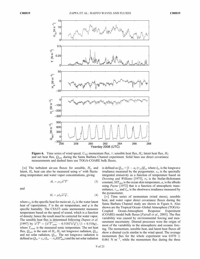
is defined as Qsw = [1� as (tes)]Isw where Ilw is the longwaveirradiance measured by the pyrgeometer, ɛsi is the spectrallyintegrated emissivity as a function of temperature based onDowning and Williams [1975], sb is the Stefan-Boltzmannconstant, SSTskin is the ocean skin temperature, as is the albedousing Payne [1972] that is a function of atmospheric trans-mittance, tes, and Isw is the shortwave irradiance measured bythe pyranometer.[31] Time series of momentum (wind stress), sensible

heat, and water vapor direct covariance fluxes during theSanta Barbara Channel study are shown in Figure 6. Alsoshown are the Tropical Ocean–Global Atmosphere (TOGA)-Coupled Ocean-Atmosphere Response Experiment(COARE) model bulk fluxes [Fairall et al., 2003]. The fluxvariability was caused by environmental forcing and mea-surement uncertainty. Diurnal processes were the origin ofmost of the variability in the atmospheric and oceanic forc-ing. The momentum, sensible heat, and latent heat fluxes allshow a diurnal cycle similar to the wind speed. The averagemomentum flux for the whole experiment was 0.070 �0.061 N m�2, while the momentum flux during the three

Figure 6. Time series of wind speed, U10; momentum flux, t; sensible heat flux, Hs; latent heat flux, Hl;and net heat flux, Qnet, during the Santa Barbara Channel experiment. Solid lines use direct covariancemeasurements and dashed lines use TOGA-COARE bulk fluxes.


9 of 23

regimes 0.062 � 0.064 (days 257–259), 0.104 � 0.062(days 260–263), and 0.042 � 0.035 N m�2 (days 264–268).The most significant diurnal process came from the seabreeze. Strong diurnal heating of the California centralvalley and high desert created a low atmospheric pressureover land, which accelerated the westerly gradient windduring the afternoon and evening. Large radiative cooling ofthe dry soil in clear skies leads to significant cooling of theterrestrial nighttime atmosphere, and consequently thepressure gradient decreases. This leads to diurnal variationsin wind speed, and hence wind stress, momentum flux andsea state. The surface ocean is heated during the day byincident solar radiation. At night, when solar radiation isnonexistent, infrared radiation, evaporation, and sensibleheat fluxes cool the ocean surface. These processes varythrough the diurnal cycle and cause subsequent processesthat change the transport of heat, mass, and momentumacross the air-sea interface. The diurnal barometric pressurechanges are small. Thus, the time series of direct covariancemeasurements are close to a uniform daily mean and banded

around variability caused by noise and diurnal forcing. Themean and standard deviation of the sensible and latent heatdirect covariance fluxes were �13.9 � 10.7 and �33.9 �21.8 W m�2. Note that the standard deviations of themeasured 0.5 h direct covariance fluxes are often as large asthe mean fluxes. For days 258–263, the mean sensible heatflux was �20.8 � 8.8 W m�2, the mean latent heat flux was�45.6 � 17.2 W m�2, and the mean net cooling at nightwas �125.6 � 38.5 W m�2. During regime three betweendays 264 and 268, the mean sensible heat flux was �6.4 �7.8Wm�2, themean latent heat flux was�21.7� 19.9Wm�2,and the mean net cooling at night was �89.3 � 16.5 W m�2.The peak warming throughout the experiment rangedbetween 600 and 750 W m�2.[32] Time series of momentum (wind stress), sensible

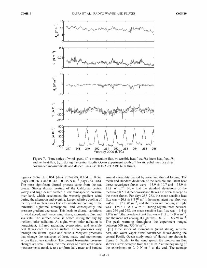
heat, and water vapor direct covariance fluxes during thecentral Pacific Ocean study south of Hawaii are shown inFigure 7. Similar to the wind speed, the momentum fluxshows a slow decrease from 0.16 N m�2 at the beginning ofthe experiment to 0.10 N m�2 at the end. The average

Figure 7. Time series of wind speed, U10; momentum flux, t; sensible heat flux, Hs; latent heat flux, Hl;and net heat flux, Qnet, during the central Pacific Ocean experiment south of Hawaii. Solid lines use directcovariance measurements and dashed lines use TOGA-COARE bulk fluxes.


10 of 23

momentum flux for the whole experiment was 0.118 �0.041 N m�2. Again, the most significant diurnal process isthe heating and cooling of the ocean surface. The mean andstandard deviation of the sensible and latent heat directcovariance fluxes were �15.1 � 5.46 and �126.9 �32.2 W m�2. The mean net cooling at night throughoutthe experiment was �190.2 � 43.35 W m�2. The peakwarming throughout the experiment ranged between 600 and780 W m�2. Note that on day 253, rain contaminated all thedirect covariance fluxes, including the net heat flux.[33] The RaDyO flux data tracks the TOGA-COARE 3.0

model prediction closely. The measured sensible heat flux iswithin 1.1 W m�2 of the TOGA-COARE 3.0 model pre-diction for SBC and within 2.1 W m�2 for the Pacific Oceansouth of Hawaii. The TOGA-COARE 3.0 model predictionoverestimates the measured latent heat flux by at most31.6% for SBC and 21.8% for the Pacific Ocean south ofHawaii. Edson [2008] has observed similar tendencies ofthis magnitude in his extensive data sets including ClivarMode Water Dynamic Experiment (CLIMODE), CoupledBoundary Layer and Air-Sea Transfer (CBLAST) Experi-ment, Marine Boundary Layer (MBL) Experiment, and RisøAir-Sea Experiment (RASEX). He is incorporating theseobservations into the latest TOGA-COARE 4.0 modeltransfer coefficients where the Dalton number needs to bereduced by up to 25% for winds below 10 m s�1 [see Edson,2008, Figure 8]. Thus, the greater overestimation observedin SBC for the latent heat flux is consistent with the largercorrections at lower wind speeds proposed by Edson [2008].Our observations during the RaDyO experiments in SBCand in the Pacific Ocean south of Hawaii provide indepen-dent validation of these effects.[34] We note that the dynamic range of the wind stress is

larger during the SBC experiment than the Hawaii experi-ment. Together these two experiments provide an interestingvariety of sea state conditions including light and variable tostrongly whitecapping. They provide a valuable test bed formean square slope and breaking measurements over aninteresting dynamic range of wind speeds.[35] The results presented here document the underlying

conditions to support the optical measurements gatheredduring RaDyO. The short duration of the RaDyO observa-tional periods results in too few data to refine or comment onthe flux parameterization relationships. Much longer recordswould have been needed to compare the transfer coefficients(Stanton and Dalton numbers) in the coastal versus openocean settings.

4.3. Wave Conditions

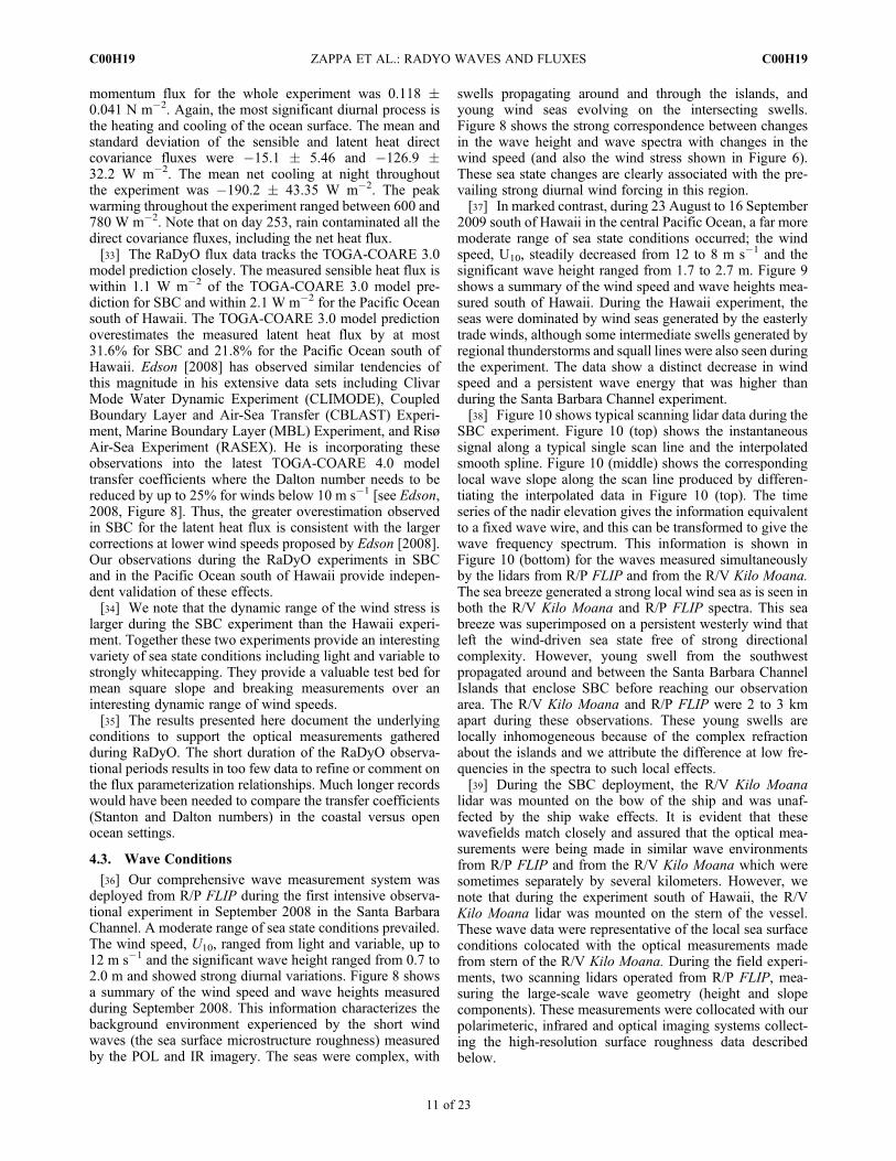
[36] Our comprehensive wave measurement system wasdeployed from R/P FLIP during the first intensive observa-tional experiment in September 2008 in the Santa BarbaraChannel. A moderate range of sea state conditions prevailed.The wind speed, U10, ranged from light and variable, up to12 m s�1 and the significant wave height ranged from 0.7 to2.0 m and showed strong diurnal variations. Figure 8 showsa summary of the wind speed and wave heights measuredduring September 2008. This information characterizes thebackground environment experienced by the short windwaves (the sea surface microstructure roughness) measuredby the POL and IR imagery. The seas were complex, with

swells propagating around and through the islands, andyoung wind seas evolving on the intersecting swells.Figure 8 shows the strong correspondence between changesin the wave height and wave spectra with changes in thewind speed (and also the wind stress shown in Figure 6).These sea state changes are clearly associated with the pre-vailing strong diurnal wind forcing in this region.[37] In marked contrast, during 23 August to 16 September

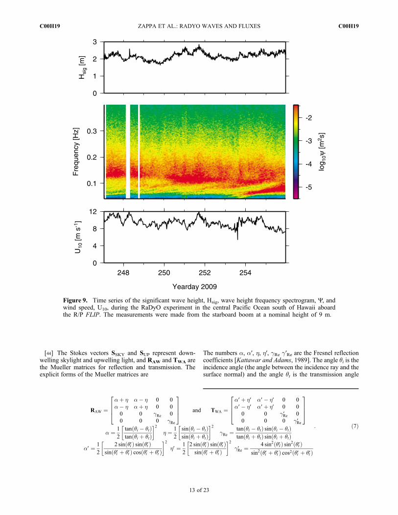
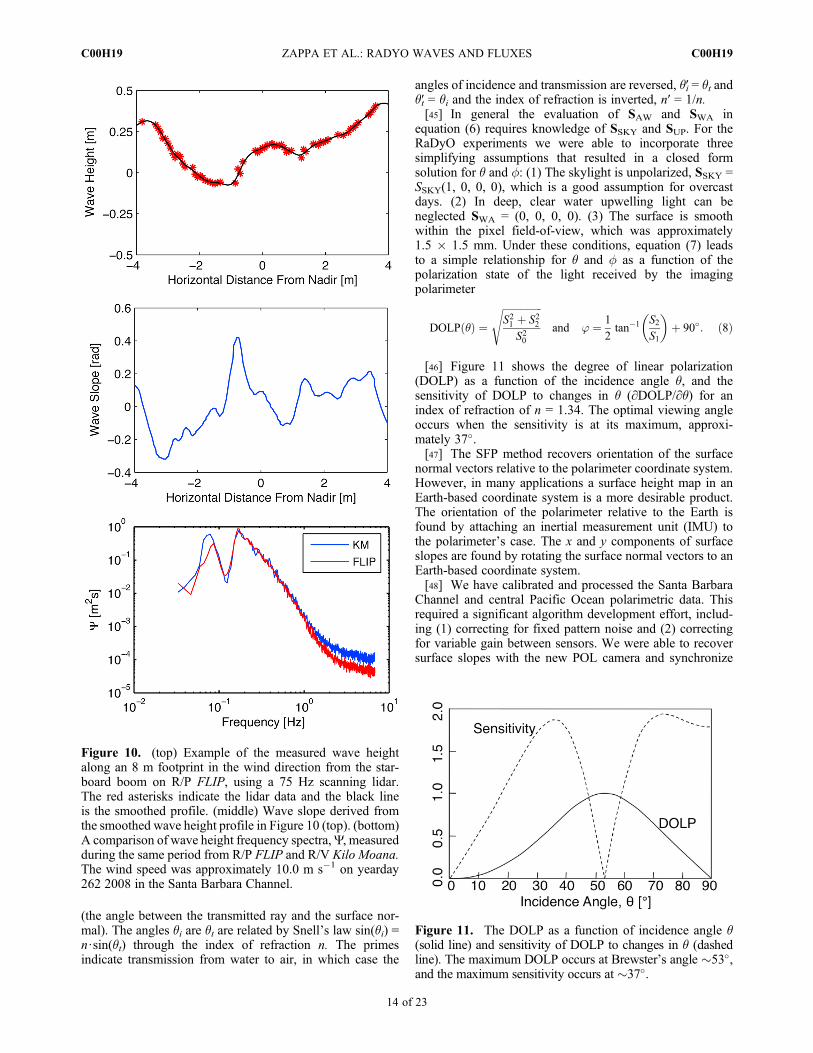
2009 south of Hawaii in the central Pacific Ocean, a far moremoderate range of sea state conditions occurred; the windspeed, U10, steadily decreased from 12 to 8 m s�1 and thesignificant wave height ranged from 1.7 to 2.7 m. Figure 9shows a summary of the wind speed and wave heights mea-sured south of Hawaii. During the Hawaii experiment, theseas were dominated by wind seas generated by the easterlytrade winds, although some intermediate swells generated byregional thunderstorms and squall lines were also seen duringthe experiment. The data show a distinct decrease in windspeed and a persistent wave energy that was higher thanduring the Santa Barbara Channel experiment.[38] Figure 10 shows typical scanning lidar data during the

SBC experiment. Figure 10 (top) shows the instantaneoussignal along a typical single scan line and the interpolatedsmooth spline. Figure 10 (middle) shows the correspondinglocal wave slope along the scan line produced by differen-tiating the interpolated data in Figure 10 (top). The timeseries of the nadir elevation gives the information equivalentto a fixed wave wire, and this can be transformed to give thewave frequency spectrum. This information is shown inFigure 10 (bottom) for the waves measured simultaneouslyby the lidars from R/P FLIP and from the R/V Kilo Moana.The sea breeze generated a strong local wind sea as is seen inboth the R/V Kilo Moana and R/P FLIP spectra. This seabreeze was superimposed on a persistent westerly wind thatleft the wind-driven sea state free of strong directionalcomplexity. However, young swell from the southwestpropagated around and between the Santa Barbara ChannelIslands that enclose SBC before reaching our observationarea. The R/V Kilo Moana and R/P FLIP were 2 to 3 kmapart during these observations. These young swells arelocally inhomogeneous because of the complex refractionabout the islands and we attribute the difference at low fre-quencies in the spectra to such local effects.[39] During the SBC deployment, the R/V Kilo Moana

lidar was mounted on the bow of the ship and was unaf-fected by the ship wake effects. It is evident that thesewavefields match closely and assured that the optical mea-surements were being made in similar wave environmentsfrom R/P FLIP and from the R/V Kilo Moana which weresometimes separately by several kilometers. However, wenote that during the experiment south of Hawaii, the R/VKilo Moana lidar was mounted on the stern of the vessel.These wave data were representative of the local sea surfaceconditions colocated with the optical measurements madefrom stern of the R/V Kilo Moana. During the field experi-ments, two scanning lidars operated from R/P FLIP, mea-suring the large-scale wave geometry (height and slopecomponents). These measurements were collocated with ourpolarimeteric, infrared and optical imaging systems collect-ing the high-resolution surface roughness data describedbelow.


11 of 23

4.4. Shape From Polarimetry

[40] The POL camera is an exciting new imaging instru-ment for detecting very short gravity waves and capillarywaves. It produces estimates of the sea surface slopetopography of a small patch of the sea surface at high reso-lution and at video rates.[41] The phase-resolved, spatial-temporal history of small

waves was measured using the shape-from-polarimetry(SFP) technique first described by Zappa et al. [2008]. TheSFP technique relates the change in polarization of skylightreflecting from water to infer the orientation of the watersurface at the point of reflection. The incident skylightstrikes the water surface at an angle q relative to the surfacenormal. The incident light ray, the surface normal and thereflected light ray form a plane, which intersects the imageplane of the polarimeter at an angle, f. The SFP methodrelates the change in polarization to the incidence angle, andthe orientation of the polarization to the tilt of the plane ofreflection.

[42] The values of (q, f) are derived from the Muellercalculus, which relates the polarization state of the incomingand scattered light through a Mueller matrix that depends onthe electrical and geometric properties of the scatteringmedia. The polarization state of a bundle of light rays isspecified by the Stokes parameters [Stokes, 1852]. The Stokesparameters form a four element vector S = (S0, S1, S2, S3),where S0 is the intensity, S1 and S2 define the state of linearpolarization, and S3 defines the degree of circular polarization.[43] The polarization state S of light reaching a polarimeter

looking at a water surface is the sum of the skylight reflectedfrom the water surface SAW and the light transmitted throughthe water surface SWA

S ¼ SAW þ SWA: ð5Þ

The values of SAW and SWA are found usingMueller calculus

SAW ¼ RAW⋅SSKY and SWA ¼ TWA⋅SUP: ð6Þ

Figure 8. Time series of the significant wave height, Hsig, wave height frequency spectrogram, Y, andwind speed, U10, during the RaDyO Santa Barbara Channel experiment aboard the R/P FLIP. The mea-surements were made from the starboard boom at a nominal height of 9 m.


12 of 23

[44] The Stokes vectors SSKY and SUP represent down-welling skylight and upwelling light, and RAW and TWA arethe Mueller matrices for reflection and transmission. Theexplicit forms of the Mueller matrices are

The numbers a, a′, h, h′, gRe g′Re are the Fresnel reflectioncoefficients [Kattawar and Adams, 1989]. The angle qi is theincidence angle (the angle between the incidence ray and thesurface normal) and the angle qt is the transmission angle

RAW ¼aþ h a� h 0 0a� h aþ h 0 00 0 gRe 00 0 0 gRe

2664

3775 and TWA ¼

a′ þ h′ a′ � h′ 0 0a′ � h′ a′ þ h′ 0 0

0 0 g′Re 00 0 0 g′Re

2664

3775

a ¼ 1

2

tan qi � qtð Þtan qi þ qtð Þ� �2

h ¼ 1

2

sin qi � qtð Þsin qi þ qtð Þ� �2

gRe ¼tan qi � qtð Þ sin qi � qtð Þtan qi þ qtð Þ sin qi þ qtð Þ

a′ ¼ 1

2

2 sin q′ið Þ sin q′tð Þsin q′i þ q′tð Þ cos q′i þ q′tð Þ� �2

h′ ¼ 1

2

2 sin q′ið Þ sin q′tð Þsin q′i þ q′tð Þ

� �2g′Re ¼

4 sin2 q′1ð Þ sin2 q′tð Þsin2 q′i þ q′tð Þ cos2 q′i þ q′tð Þ

: ð7Þ

Figure 9. Time series of the significant wave height, Hsig, wave height frequency spectrogram, Y, andwind speed, U10, during the RaDyO experiment in the central Pacific Ocean south of Hawaii aboardthe R/P FLIP. The measurements were made from the starboard boom at a nominal height of 9 m.


13 of 23

(the angle between the transmitted ray and the surface nor-mal). The angles qi are qt are related by Snell’s law sin(qi) =n⋅sin(qt) through the index of refraction n. The primesindicate transmission from water to air, in which case the

angles of incidence and transmission are reversed, q′i = qt andq′t = qi and the index of refraction is inverted, n′ = 1/n.[45] In general the evaluation of SAW and SWA in

equation (6) requires knowledge of SSKY and SUP. For theRaDyO experiments we were able to incorporate threesimplifying assumptions that resulted in a closed formsolution for q and f: (1) The skylight is unpolarized, SSKY =SSKY(1, 0, 0, 0), which is a good assumption for overcastdays. (2) In deep, clear water upwelling light can beneglected SWA = (0, 0, 0, 0). (3) The surface is smoothwithin the pixel field-of-view, which was approximately1.5 � 1.5 mm. Under these conditions, equation (7) leadsto a simple relationship for q and f as a function of thepolarization state of the light received by the imagingpolarimeter

DOLP qð Þ ¼ffiffiffiffiffiffiffiffiffiffiffiffiffiffiffiffiS21 þ S22

S20

sand j ¼ 1

2tan�1 S2

S1

� �þ 90�: ð8Þ

[46] Figure 11 shows the degree of linear polarization(DOLP) as a function of the incidence angle q, and thesensitivity of DOLP to changes in q (∂DOLP/∂q) for anindex of refraction of n = 1.34. The optimal viewing angleoccurs when the sensitivity is at its maximum, approxi-mately 37�.[47] The SFP method recovers orientation of the surface

normal vectors relative to the polarimeter coordinate system.However, in many applications a surface height map in anEarth-based coordinate system is a more desirable product.The orientation of the polarimeter relative to the Earth isfound by attaching an inertial measurement unit (IMU) tothe polarimeter’s case. The x and y components of surfaceslopes are found by rotating the surface normal vectors to anEarth-based coordinate system.[48] We have calibrated and processed the Santa Barbara

Channel and central Pacific Ocean polarimetric data. Thisrequired a significant algorithm development effort, includ-ing (1) correcting for fixed pattern noise and (2) correctingfor variable gain between sensors. We were able to recoversurface slopes with the new POL camera and synchronize

Figure 10. (top) Example of the measured wave heightalong an 8 m footprint in the wind direction from the star-board boom on R/P FLIP, using a 75 Hz scanning lidar.The red asterisks indicate the lidar data and the black lineis the smoothed profile. (middle) Wave slope derived fromthe smoothed wave height profile in Figure 10 (top). (bottom)A comparison of wave height frequency spectra,Y, measuredduring the same period from R/P FLIP and R/V Kilo Moana.The wind speed was approximately 10.0 m s�1 on yearday262 2008 in the Santa Barbara Channel.

Figure 11. The DOLP as a function of incidence angle q(solid line) and sensitivity of DOLP to changes in q (dashedline). The maximum DOLP occurs at Brewster’s angle �53�,and the maximum sensitivity occurs at �37�.


14 of 23

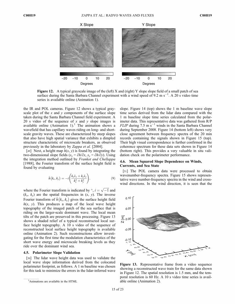
the IR and POL cameras. Figure 12 shows a typical gray-scale plot of the x and y components of the surface slopetaken during the Santa Barbara Channel field experiment. A20 s video of the sequence of x and y slope images isavailable online (Animation 1).1 The animation shows awavefield that has capillary waves riding on long- and short-scale gravity waves. These are characterized by steep slopesthat also have high spatial variance that exhibits a dimpledstructure characteristic of microscale breakers, as observedpreviously in the laboratory by Zappa et al. [2004].[49] Next, a height map h(x, y) is found by integrating the

two-dimensional slope fields (sx = ∂h/∂x, sy = ∂h/∂y). Usingthe integration method outlined by Frankot and Chellappa[1988], the Fourier transform of the surface height field isfound by evaluating

h kx; ky� � ¼ �i

kxsx þ kysyk2x þ k2y

!; ð9Þ

where the Fourier transform is indicated by ^, i ¼ ffiffiffiffiffiffiffi�1p

and(kx, ky) are the spatial frequencies in (x, y). The inverseFourier transform of h kx; ky

� �gives the surface height field

h(x, y). This produces a map of the local wave heighttopography of the imaged patch of the sea surface that isriding on the larger-scale dominant wave. The local meantilts of the patch are preserved in this processing. Figure 13shows a shaded relief of a typical reconstructed local sur-face height topography. A 10 s video of the sequence ofreconstructed local surface height topography is availableonline (Animation 2). Such reconstructions allow investi-gating for the first time the modulation characteristics of theshort wave energy and microscale breaking levels as theyride over the dominant wind sea.

4.5. Polarimeter Slope Validation

[50] The lidar wave height data was used to validate thelocal wave slope information derived from the colocatedpolarimeter footprint, as follows. A 1 m baseline was chosenfor this task to minimize the errors in the lidar-inferred wave

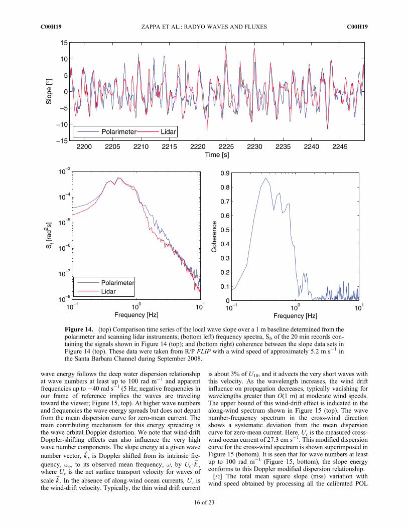
slope. Figure 14 (top) shows the 1 m baseline wave slopetime series derived from the lidar data compared with the1 m baseline slope time series calculated from the polar-imeter data. This representative data was gathered from R/PFLIP during 7.5 m s�1 winds in the Santa Barbara Channelduring September 2008. Figure 14 (bottom left) shows veryclose agreement between frequency spectra of the 20 minrecords containing the signals shown in Figure 15 (top).Their high visual correspondence is further confirmed in thecoherence spectrum for these data sets shown in Figure 14(bottom right). This provides a very valuable in situ vali-dation check on the polarimeter performance.

4.6. Mean Squared Slope Dependence on Winds,Currents, and Sea State

[51] The POL camera data were processed to obtainwavenumber-frequency spectra. Figure 15 shows represen-tative wave number-frequency spectra in the wind and cross-wind directions. In the wind direction, it is seen that the

Figure 12. A typical grayscale image of the (left) X and (right) Y slope slope field of a small patch of seasurface during the Santa Barbara Channel experiment with a wind speed of 9.2 m s�1. A 20 s video timeseries is available online (Animation 1).

Figure 13. Representative frame from a video sequenceshowing a reconstructed wave train for the same data shownin Figure 12. The spatial resolution is 1.5 mm, and the tem-poral resolution is 60 Hz. A 10 s video time series is avail-able online (Animation 2).1Animations are available in the HTML


15 of 23

wave energy follows the deep water dispersion relationshipat wave numbers at least up to 100 rad m�1 and apparentfrequencies up to �40 rad s�1 (5 Hz; negative frequencies inour frame of reference implies the waves are travelingtoward the viewer; Figure 15, top). At higher wave numbersand frequencies the wave energy spreads but does not departfrom the mean dispersion curve for zero-mean current. Themain contributing mechanism for this energy spreading isthe wave orbital Doppler distortion. We note that wind-driftDoppler-shifting effects can also influence the very highwave number components. The slope energy at a given wavenumber vector, ~k , is Doppler shifted from its intrinsic fre-quency, wo, to its observed mean frequency, w, by Uc⋅~k ,where Uc is the net surface transport velocity for waves ofscale ~k . In the absence of along-wind ocean currents, Uc isthe wind-drift velocity. Typically, the thin wind drift current

is about 3% of U10, and it advects the very short waves withthis velocity. As the wavelength increases, the wind driftinfluence on propagation decreases, typically vanishing forwavelengths greater than O(1 m) at moderate wind speeds.The upper bound of this wind-drift effect is indicated in thealong-wind spectrum shown in Figure 15 (top). The wavenumber-frequency spectrum in the cross-wind directionshows a systematic deviation from the mean dispersioncurve for zero-mean current. Here, Uc is the measured cross-wind ocean current of 27.3 cm s�1. This modified dispersioncurve for the cross-wind spectrum is shown superimposed inFigure 15 (bottom). It is seen that for wave numbers at leastup to 100 rad m�1 (Figure 15, bottom), the slope energyconforms to this Doppler modified dispersion relationship.[52] The total mean square slope (mss) variation with

wind speed obtained by processing all the calibrated POL

Figure 14. (top) Comparison time series of the local wave slope over a 1 m baseline determined from thepolarimeter and scanning lidar instruments; (bottom left) frequency spectra, Sf, of the 20 min records con-taining the signals shown in Figure 14 (top); and (bottom right) coherence between the slope data sets inFigure 14 (top). These data were taken from R/P FLIP with a wind speed of approximately 5.2 m s�1 inthe Santa Barbara Channel during September 2008.


16 of 23

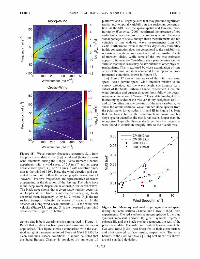
camera data in both experiments is summarized in Figure 16.Recall that all data has been processed assuming the sky isunpolarized. This figure shows a comparison with the clas-sical sun glint parameterization of Cox and Munk [1956] forclean and slick surface conditions. It should be noted thatthe Santa Barbara Channel is populated by numerous oil

platforms and oil seepage sites that may produce significantspatial and temporal variability in the surfactant concentra-tion. At the SBC site, the sparse spatial and temporal mon-itoring by Wurl et al. [2009] confirmed the presence of lowsurfactant concentrations in the microlayer and the occa-sional passage of slicks, though these measurements did notcoincide in time with our wave measurements from R/PFLIP. Furthermore, even as the weak day-to-day variabilityin this concentration does not correspond to the variability inour mss observations, we cannot rule out the possible effectsof transient slicks. While some of the low mss estimatesappear to lie near the Cox-Munk slick parameterization, wesurmise that these cases may be attributable to other physicalmechanisms. This is explored by close examination of timeseries of the mss variation compared to the operative envi-ronmental conditions shown in Figure 17.[53] Figure 17 shows time series of the total mss, wind

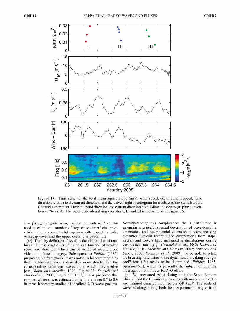
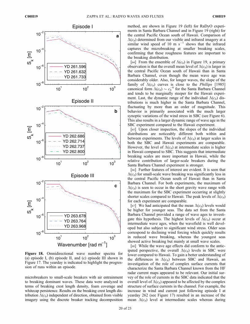
speed, ocean current speed, wind direction relative to thecurrent direction, and the wave height spectrogram for asubset of the Santa Barbara Channel experiment. Here, thewind direction and current direction both follow the ocean-ographic convention of “toward.” These data highlight threeinteresting episodes of the mss variability designated as I, II,and III. To refine our interpretation of the mss variability, weshow the omnidirectional wave number slope spectra fromthe polarimeter for episodes I, II, and III in Figure 18. Notethat the lowest bin of the omnidirectional wave numberslope spectra quantifies the mss for all scales longer than theimage size. Typically, these scales larger than the image sizewere found to contribute roughly 20% to the overall mss.

Figure 15. Wave number–frequency spectrum, Skw, fromthe polarimeter data in the (top) wind and (bottom) cross-wind directions during the RaDyO Santa Barbara Channelexperiment with a wind speed of 5.5 m s�1 and an upperocean current speed, Uc, of 27.3 cm s�1 with a relative direc-tion to the wind of 110�. Here, the wind direction and cur-rent direction both follow the oceanographic convention of“toward.” Positive frequencies are representative of wavespropagating in the direction of the forcing. The white traceis the deep water dispersion relationship for ocean waves.The black trace shows that a given wave number vector, ~k ,is Doppler shifted from its intrinsic frequency, wo, to itsobserved mean frequency, w, by Uc⋅~k , where Uc is the netsurface transport velocity for waves of scale ~k . In theabsence of along-wind ocean currents, Uc is the wind-driftvelocity (Figure 15, top) and Uc is the measured cross-windocean current (Figure 15, bottom).

Figure 16. Mean squared total slope against wind speedduring the Santa Barbara Channel and Hawaii RaDyO fieldexperiments. The red symbols represent episode I, the bluesymbols represent episode II, green symbols representepisode III, and the black symbols represent the rest of thepolarimeter data. The solid and dashed lines represent theCox and Munk [1956] best linear fits to their clean surfaceand slick-covered surface results, respectively. The errorbounds to the Cox and Munk [1956] best linear fits shownare �1 standard deviation.


17 of 23

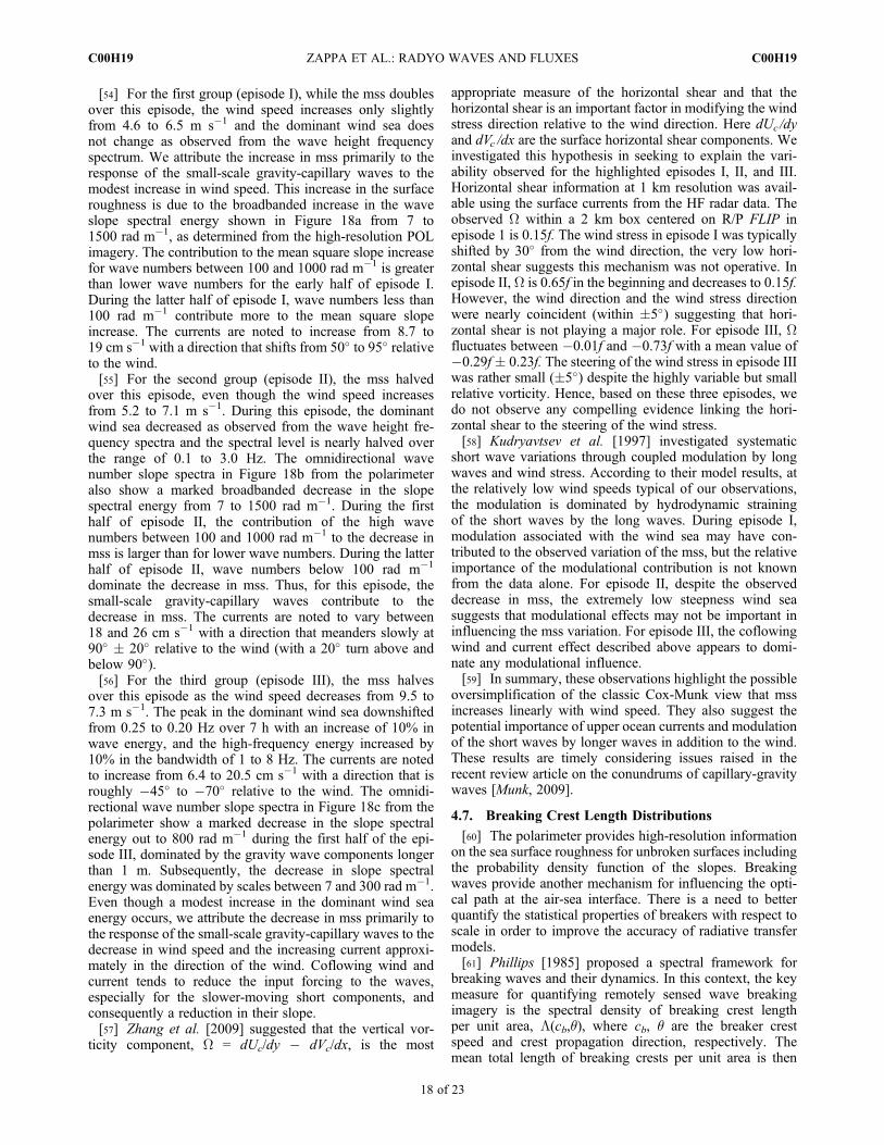
[54] For the first group (episode I), while the mss doublesover this episode, the wind speed increases only slightlyfrom 4.6 to 6.5 m s�1 and the dominant wind sea doesnot change as observed from the wave height frequencyspectrum. We attribute the increase in mss primarily to theresponse of the small-scale gravity-capillary waves to themodest increase in wind speed. This increase in the surfaceroughness is due to the broadbanded increase in the waveslope spectral energy shown in Figure 18a from 7 to1500 rad m�1, as determined from the high-resolution POLimagery. The contribution to the mean square slope increasefor wave numbers between 100 and 1000 rad m�1 is greaterthan lower wave numbers for the early half of episode I.During the latter half of episode I, wave numbers less than100 rad m�1 contribute more to the mean square slopeincrease. The currents are noted to increase from 8.7 to19 cm s�1 with a direction that shifts from 50� to 95� relativeto the wind.[55] For the second group (episode II), the mss halved

over this episode, even though the wind speed increasesfrom 5.2 to 7.1 m s�1. During this episode, the dominantwind sea decreased as observed from the wave height fre-quency spectra and the spectral level is nearly halved overthe range of 0.1 to 3.0 Hz. The omnidirectional wavenumber slope spectra in Figure 18b from the polarimeteralso show a marked broadbanded decrease in the slopespectral energy from 7 to 1500 rad m�1. During the firsthalf of episode II, the contribution of the high wavenumbers between 100 and 1000 rad m�1 to the decrease inmss is larger than for lower wave numbers. During the latterhalf of episode II, wave numbers below 100 rad m�1

dominate the decrease in mss. Thus, for this episode, thesmall-scale gravity-capillary waves contribute to thedecrease in mss. The currents are noted to vary between18 and 26 cm s�1 with a direction that meanders slowly at90� � 20� relative to the wind (with a 20� turn above andbelow 90�).[56] For the third group (episode III), the mss halves

over this episode as the wind speed decreases from 9.5 to7.3 m s�1. The peak in the dominant wind sea downshiftedfrom 0.25 to 0.20 Hz over 7 h with an increase of 10% inwave energy, and the high-frequency energy increased by10% in the bandwidth of 1 to 8 Hz. The currents are notedto increase from 6.4 to 20.5 cm s�1 with a direction that isroughly �45� to �70� relative to the wind. The omnidi-rectional wave number slope spectra in Figure 18c from thepolarimeter show a marked decrease in the slope spectralenergy out to 800 rad m�1 during the first half of the epi-sode III, dominated by the gravity wave components longerthan 1 m. Subsequently, the decrease in slope spectralenergy was dominated by scales between 7 and 300 rad m�1.Even though a modest increase in the dominant wind seaenergy occurs, we attribute the decrease in mss primarily tothe response of the small-scale gravity-capillary waves to thedecrease in wind speed and the increasing current approxi-mately in the direction of the wind. Coflowing wind andcurrent tends to reduce the input forcing to the waves,especially for the slower-moving short components, andconsequently a reduction in their slope.[57] Zhang et al. [2009] suggested that the vertical vor-

ticity component, W = dUc/dy � dVc/dx, is the most

appropriate measure of the horizontal shear and that thehorizontal shear is an important factor in modifying the windstress direction relative to the wind direction. Here dUc/dyand dVc /dx are the surface horizontal shear components. Weinvestigated this hypothesis in seeking to explain the vari-ability observed for the highlighted episodes I, II, and III.Horizontal shear information at 1 km resolution was avail-able using the surface currents from the HF radar data. Theobserved W within a 2 km box centered on R/P FLIP inepisode 1 is 0.15f. The wind stress in episode I was typicallyshifted by 30� from the wind direction, the very low hori-zontal shear suggests this mechanism was not operative. Inepisode II, W is 0.65f in the beginning and decreases to 0.15f.However, the wind direction and the wind stress directionwere nearly coincident (within �5�) suggesting that hori-zontal shear is not playing a major role. For episode III, Wfluctuates between �0.01f and �0.73f with a mean value of�0.29f� 0.23f. The steering of the wind stress in episode IIIwas rather small (�5�) despite the highly variable but smallrelative vorticity. Hence, based on these three episodes, wedo not observe any compelling evidence linking the hori-zontal shear to the steering of the wind stress.[58] Kudryavtsev et al. [1997] investigated systematic

short wave variations through coupled modulation by longwaves and wind stress. According to their model results, atthe relatively low wind speeds typical of our observations,the modulation is dominated by hydrodynamic strainingof the short waves by the long waves. During episode I,modulation associated with the wind sea may have con-tributed to the observed variation of the mss, but the relativeimportance of the modulational contribution is not knownfrom the data alone. For episode II, despite the observeddecrease in mss, the extremely low steepness wind seasuggests that modulational effects may not be important ininfluencing the mss variation. For episode III, the coflowingwind and current effect described above appears to domi-nate any modulational influence.[59] In summary, these observations highlight the possible

oversimplification of the classic Cox-Munk view that mssincreases linearly with wind speed. They also suggest thepotential importance of upper ocean currents and modulationof the short waves by longer waves in addition to the wind.These results are timely considering issues raised in therecent review article on the conundrums of capillary-gravitywaves [Munk, 2009].

4.7. Breaking Crest Length Distributions

[60] The polarimeter provides high-resolution informationon the sea surface roughness for unbroken surfaces includingthe probability density function of the slopes. Breakingwaves provide another mechanism for influencing the opti-cal path at the air-sea interface. There is a need to betterquantify the statistical properties of breakers with respect toscale in order to improve the accuracy of radiative transfermodels.[61] Phillips [1985] proposed a spectral framework for

breaking waves and their dynamics. In this context, the keymeasure for quantifying remotely sensed wave breakingimagery is the spectral density of breaking crest lengthper unit area, L(cb,q), where cb, q are the breaker crestspeed and crest propagation direction, respectively. Themean total length of breaking crests per unit area is then


18 of 23

L =RL(cb, q)dcb dq. Also, various moments of L can be

used to estimate a number of key air-sea interfacial prop-erties, including swept whitecap area with respect to scale,whitecap cover and the upper ocean dissipation rate.[62] Thus, by definition, L(cb,q) is the distribution of total

breaking crest lengths per unit area as a function of breakerspeed and direction, which can be extracted readily fromvideo or infrared imagery. Subsequent to Phillips [1985]proposing his framework, it was noted in laboratory studiesthat the breakers travel measurably more slowly than thecorresponding unbroken waves from which they evolve[e.g., Rapp and Melville, 1990, Figure 33; Stansell andMacFarlane, 2002, Figure 5]. Thus, it was proposed thatcb = ac, where a was estimated to lie in the range 0.7 to 0.9in these laboratory studies of idealized 2-D wave packets.

Notwithstanding this complication, the L distribution isemerging as a useful spectral description of wave-breakingkinematics, and has potential extension to wave-breakingdynamics. Several recent video observations from ships,aircraft and towers have measured L distributions duringvarious sea states [e.g., Gemmrich et al., 2008; Kleiss andMelville, 2010; Melville and Matusov, 2002; Mironov andDulov, 2008; Thomson et al., 2009]. To be able to relatethe breaking kinematics to the dynamics, a breaking strengthcoefficient (‘b’) needs to be determined [Phillips, 1985,equation 6.3], which is presently the subject of ongoinginvestigation within our RaDyO effort.[63] We measured L(cb) during both the Santa Barbara

Channel and the Hawaii experiments with our suite of videoand infrared cameras mounted on R/P FLIP. The scale ofwave breaking during both field experiments ranged from

Figure 17. Time series of the total mean square slope (mss), wind speed, ocean current speed, winddirection relative to the current direction, and the wave height spectrogram for a subset of the Santa BarbaraChannel experiment. Here the wind direction and current direction both follow the oceanographic conven-tion of “toward.” The color code identifying episodes I, II, and III is the same as in Figure 16.


19 of 23

microbreakers to small-scale breakers with air entrainmentto breaking dominant waves. These data were analyzed interms of breaking crest length density, foam coverage andwhitecap persistence. Results on the breaking crest length dis-tribution L(cb) independent of direction, obtained from visibleimagery using the discrete breaker tracking decomposition

method, are shown in Figure 19 (left) for RaDyO experi-ments in Santa Barbara Channel and in Figure 19 (right) forthe central Pacific Ocean south of Hawaii. Comparison ofL(cb) determined from our visible and infrared imagery at asimilar wind speed of 10 m s�1 shows that the infraredcaptures the microbreaking at smaller breaking scales,confirming that these roughness features are important tothe breaking distribution.[64] From the ensemble of L(cb) in Figure 19, a primary

observation is that the overall mean level of L(cb) is larger inthe central Pacific Ocean south of Hawaii than in SantaBarbara Channel, even though the mean wave age wasconsiderably older. Also, for longer waves, the slope of thefamily of L(cb) curves is close to the Phillips [1985]canonical form L(cb) � cb

�6 for the Santa Barbara Channeland tends to be marginally steeper for the Hawaii experi-ment. Last, the dynamic range of the individual L(cb) dis-tributions is much higher in the Santa Barbara Channel,fluctuating by more than an order of magnitude. Thisbehavior is primarily associated with the much largersynoptic variations of the wind stress in SBC (see Figure 6).This also results in a larger dynamic range of wave age in theSBC experiment compared to the Hawaii experiment.[65] Upon closer inspection, the slopes of the individual

distributions are noticeably different both within andbetween experiments. The levels of L(cb) at larger scales inboth the SBC and Hawaii experiments are comparable.However, the level of L(cb) at intermediate scales is higherin Hawaii compared to SBC. This suggests that intermediatebreaking scales are more important in Hawaii, while therelative contribution of larger-scale breakers during theSanta Barbara Channel experiment is stronger.[66] Further features of interest are evident. It is seen that

L(cb) for small-scale wave breaking was significantly less inthe central Pacific Ocean south of Hawaii than in SantaBarbara Channel. For both experiments, the maximum ofL(cb) is seen to occur in the short gravity wave range withthe maximum for the SBC experiment occurring at slightlyshorter scales compared to Hawaii. The peak levels of L(cb)for each experiment are comparable.[67] We had anticipated that the mean L(cb) levels would

be higher for younger seas. The data set from the SantaBarbara Channel provided a range of wave ages to investi-gate this hypothesis. The highest levels of L(cb) occur atintermediate wave ages, when the wavefield is well devel-oped but also subject to significant wind stress. Older seascorrespond to declining wind forcing which quickly resultsin reduced wave breaking, whereas the youngest seasshowed active breaking but mainly at small wave scales.[68] While the wave age effects did conform to the antic-

ipated perspective, the overall L(cb) levels in SBC werelower compared to Hawaii. To gain a better understanding ofthe differences in L(cb) between SBC and Hawaii, aninvestigation of the role of complex surface currents thatcharacterize the Santa Barbara Channel known from the HFradar current maps appeared to be relevant. Our initial sur-vey of the role of currents in the SBC data indicated that theoverall level of L(cb) appeared to be affected by the complexstructure of surface currents in the channel. For example, theincrease in wind and current just following episode I atyearday 262 (see Figure 17) resulted in an increase of themean L(cb) level at intermediate scales whereas during

Figure 18. Omnidirectional wave number spectra for(a) episode I, (b) episode II, and (c) episode III shown inFigure 17. The yearday is indicated to highlight the progres-sion of runs within an episode.


20 of 23

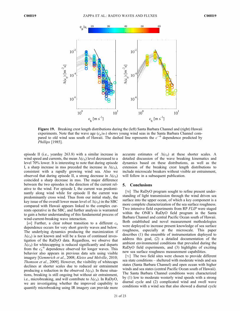
episode II (i.e., yearday 263.8) with a similar increase inwind speed and currents, the mean L(cb) level decreased to alevel 70% lower. It is interesting to note that during episodeI, a sharp increase in mss preceded the increase in L(cb),consistent with a rapidly growing wind sea. Also weobserved that during episode II, a strong decrease in L(cb)coincided a sharp decrease in mss. The major differencebetween the two episodes is the direction of the current rel-ative to the wind. For episode I, the current was predomi-nantly along wind while for episode II the current waspredominantly cross wind. Thus from our initial study, thekey issue of the overall lower mean level of L(cb) in the SBCcompared with Hawaii appears linked to the complex cur-rents operative in the SBC, and further analysis is warrantedto gain a better understanding of this fundamental process ofwind-current-breaking wave interaction.[69] Further, a clear robust transition to a different cb

dependence occurs for very short gravity waves and below.The underlying dynamics producing the maximization ifL(cb) is not known and will be a focus of continued inves-tigation of the RaDyO data. Regardless, we observe thatL(cb) for whitecapping is reduced significantly and departsfrom the cb

�6 dependence observed for longer waves. Thisbehavior also appears in previous data sets using visibleimagery [Gemmrich et al., 2008; Kleiss and Melville, 2010;Thomson et al., 2009]. However, the visibility of whitecapsdeclines at shorter scales due to reduced air entrainmentproducing a reduction in the observed L(cb). In these situa-tions, breaking is still ongoing but without air entrainment,i.e., microbreaking, and will contribute to L(cb). In RaDyO,we are investigating whether the improved capability toquantify microbreaking using IR imagery can provide more

accurate estimates of L(cb) at these shorter scales. Adetailed discussion of the wave breaking kinematics anddynamics based on these distributions, as well as theextension of the breaking crest length distributions toinclude microscale breakers without visible air entrainment,will follow in a subsequent publication.

5. Conclusions

[70] The RaDyO program sought to refine present under-standing of light transmission through the wind driven seasurface into the upper ocean, of which a key component is amore complete characterization of the sea surface roughness.Two intensive field experiments from RP FLIP were stagedwithin the ONR’s RaDyO field program in the SantaBarbara Channel and central Pacific Ocean south of Hawaii.Both established and novel measurement methodologieswere deployed to increase present knowledge of sea surfaceroughness, especially at the microscale. This paperdescribes (1) the ensemble of instrumentation deployed toaddress this goal, (2) a detailed documentation of theambient environmental conditions that prevailed during theRaDyO field experiments, and (3) highlights of excitingnew sea surface roughness measurement capabilities.[71] The two field sites were chosen to provide different

sea state conditions – sheltered with moderate winds and seastates (Santa Barbara Channel) and open ocean with higherwinds and sea states (central Pacific Ocean south of Hawaii).The Santa Barbara Channel conditions were characterizedby (1) low to moderate westerly wind speeds with a strongdiurnal cycle and (2) complicated wind and swell waveconditions with a wind sea that also showed a diurnal cycle

Figure 19. Breaking crest length distributions during the (left) Santa Barbara Channel and (right) Hawaiiexperiments. Note that the wave age (cp/u*) shows young wind seas in the Santa Barbara Channel com-pared to old wind seas south of Hawaii. The dashed line represents the c�6 dependence predicted byPhillips [1985].


21 of 23

and an average significant wave height of 1.1 � 0.3 m. Theconditions in the central Pacific Ocean south of Hawaii werecharacterized by (1) moderate easterly wind speeds thatdecreased slowly during the experiment and (2) a steadywavefield with higher overall peak wave energy comparedto Santa Barbara Channel and a significant wave height thataveraged 2.2 � 0.2 m.[72] Our observations during the RaDyO experiments are

consistent with the measurements reported by Edson [2008]from similar fixed or stable platforms such as R/P FLIP. TheTOGA-COARE 3.0 model prediction overestimates themeasured latent heat flux for SBC and for the Pacific Oceansouth of Hawaii. Edson [2008] has suggested the need toupdate the model transfer coefficients including a reduction inthe Dalton number by up to 25% for winds below 10 m s�1.Thus, our measurements would be within 5% of the newTOGA-COARE model estimates.[73] The observations gathered comprised standard marine

environmental variables (winds, waves and fluxes). Ourroughness measurements were highlighted by the first fielddeployment of our polarimeter for detecting wavefieldsdown to 1.5 mm wavelengths at sample rates up to 60 Hz.These high-resolution measurements were complemented bycolocated scanning and fixed lidars. In addition, colocatedvideo and infrared imagery gave an unprecedented coverageof the sea surface microstructure including breaking waves,over a range of wind speeds and underlying sea states. Thispaper highlights the experimental conditions and typical dataproducts derived successfully during our RaDyO study.[74] For instance, a new polarimetric imaging camera

highlights the complex interplay of processes in shaping theroughness of the sea surface. These small-scale slopeobservations by polarimetry highlight the possible over-simplification of the classic Cox-Munk view that mssincreases linearly with wind speed. They suggest thepotential importance of upper ocean currents in addition tothe wind. These results are timely considering issues raisedin the recent review article on the conundrums of capillary-gravity waves [Munk, 2009].[75] In addition, the breaking crest length spectral density

derived from visible and infrared imagery is shown to bemodulated by the development of the wavefield (wave age)and alignment of the wind and surface currents at the inter-mediate (dominant) scale of wave breaking. A primaryobservation is that the overall mean level of L(cb) is larger inthe central Pacific Ocean south of Hawaii than in SantaBarbara Channel, even though the mean wave age wasconsiderably older. While the wave age effects did conformto the anticipated perspective within each RaDyO experi-ment, the overall lower mean level of L(cb) in the SBCcompared with Hawaii appears linked to the complex cur-rents operative in the SBC. Further analysis is warranted togain a better understanding of this fundamental process ofwind-current-breaking wave interaction.

[76] Acknowledgments. We thank the captains and crews of the R/PFLIP and the R/V Kilo Moana for their invaluable assistance during ourfield operations in the Santa Barbara Channel and south of Hawaiiand L. Pezzaniti of Polaris Sensor Technologies for his expertise in thedevelopment of the imaging polarimeter. We greatly appreciate theinsightful suggestions of the reviewers which we believe have enhancedthe scientific impact of the paper. The authors gratefully acknowledgesupport of this work by the Office of Naval Research under the Radiancein a Dynamic Ocean (RaDyO) DRI. C.J. Zappa and D.A. LeBel were

funded under grants N00014-06-1-0372 and N00014-11-1-0168. J. Gemmrichwas funded under grant N00014-07-1-0015. R. Morison and M. Bannerwere funded under grant N00014-06-1-0047. H. Schultz was funded undergrant N00014-07-1-0010. T. Dickey was funded from ONR’s RaDyOcontract N00014-07-1-0732 and grant N00014-08-1-1178 for his ONRSecretary of the Navy/Chief of Naval Operations Chair in OceanographicSciences for F. Nencioli, S. Jiang, D. Manov, and himself. H. Schultzdesigned and built the imaging polarimeter in cooperation with PolarisSensor Technologies with funding from the DURIP program at the Officeof Naval Research under grant N00014-07-1-0731. This is Lamont-Doherty Earth Observatory contribution 7535.

ReferencesBanner, M. L., and D. H. Peregrine (1993), Wave breaking in deep water,Annu. Rev. Fluid Mech., 25, 373–397, doi:10.1146/annurev.fl.25.010193.002105.

Businger, J. A., and A. C. Delaney (1990), Chemical sensor resolutionrequired for measuring surface fluxes by three commonmicrometeorologicaltechniques, J. Atmos. Chem., 10, 399–410, doi:10.1007/BF00115782.

Cox, C., and W. Munk (1954a), Measurement of the roughness of the seasurface from photographs of the sun’s glitter, J. Opt. Soc. Am., 44(11),838–850, doi:10.1364/JOSA.44.000838.

Cox, C., and W. Munk (1954b), Statistics of the sea surface derived fromsun glitter, J. Mar. Res., 13(2), 198–227.

Cox, C., and W. Munk (1956), Slopes of the sea surface deduced fromphotographs of sun glitter, Bull. Scripps Inst. Oceanogr., 6(9), 401–487.

Dorman, C. E., and D. Koračin (2008), Response of the summer marinelayer flow to an extreme California coastal bend, Mon. Weather Rev.,136, 2894–2992, doi:10.1175/2007MWR2336.1.

Dorman, C. E., and C. D. Winant (1995), Buoy observations of the atmo-sphere along the west coast of the United States, 1981–1990, J. Geophys.Res., 100, 16,029–16,044.

Dorman, C. E., and C. D. Winant (2000), The structure and variability ofthe marine atmosphere around the Santa Barbara Channel, Mon. WeatherRev., 128, 261–282, doi:10.1175/1520-0493(2000)128<0261:TSAVOT>2.0.CO;2.

Downing, H. D., and D. Williams (1975), Optical constants of water in theinfrared, J. Geophys. Res., 80(12), 1656–1661, doi:10.1029/JC080i012p01656.

Drennan, W. M., K. K. Kahma, and M. A. Donelan (1999), On momentumflux and velocity spectra over waves, Boundary Layer Meteorol., 92,489–515, doi:10.1023/A:1002054820455.

Dupuis, H., P. K. Taylor, A. Weill, and K. Katsaros (1997), Inertial dissipa-tion method applied to derive turbulent fluxes over the ocean during theSurface of the Ocean, Fluxes and Interactions with the Atmosphere/Atlantic Stratocumulus Transition Experiment (SOFIA/ASTEX) andStructure des Echanges Mer-Atmosphère, Propriétés des HétérogénéitésOcéaniques: Recherche Experimentale (SEMAPHORE) experimentswith low to moderate wind speeds, J. Geophys. Res., 102(C9),21,115–21,129, doi:10.1029/97JC00446.

Edson, J. B. (2008), Review of air-sea transfer processes, in Proceedings of theECMWF Workshop on Ocean-Atmosphere Interactions: 10–12 November2008, pp. 7–25, Eur. Cent. for Medium Range Forecasts, Reading, U. K.

Edson, J. B., A. A. Hinton, K. E. Prada, J. E. Hare, and C. W. Fairall(1998), Direct covariance flux estimates from mobile platforms at sea,J. Atmos. Oceanic Technol., 15(2), 547–562, doi:10.1175/1520-0426(1998)015<0547:DCFEFM>2.0.CO;2.

Fairall, C. W., E. F. Bradley, J. E. Hare, A. A. Grachev, and J. B. Edson(2003), Bulk parameterization of air-sea fluxes: Updates and verificationfor the COARE algorithm, J. Clim., 16, 571–591, doi:10.1175/1520-0442(2003)016<0571:BPOASF>2.0.CO;2.

Frankot, R. T., and R. Chellappa (1988), A method for enforcing integrabilityin shape from shading algorithms, IEEE Trans. Pattern Anal. Mach. Intell.,10(4), 439–451, doi:10.1109/34.3909.

Gemmrich, J. R., M. L. Banner, and C. Garrett (2008), Spectrally resolvedenergy dissipation and momentum flux of breaking waves, J. Phys. Ocea-nogr., 38, 1296–1312, doi:10.1175/2007JPO3762.1.

Hara, T., E. J. Bock, J. B. Edson, and W. R. McGillis (1998), Observationof short wind waves in coastal waters, J. Phys. Oceanogr., 28(7),1425–1438, doi:10.1175/1520-0485(1998)028<1425:OOSWWI>2.0.CO;2.

Hara, T., K. A. Hanson, E. J. Bock, and B. M. Uz (2003), Observation ofhydrodynamic modulation of gravity-capillary waves by dominant gravitywaves, J. Geophys. Res., 108(C2), 3028, doi:10.1029/2001JC001100.

Hellerman, S., and M. Rosenstein (1983), Normal monthly wind stress overthe world ocean with error estimates, J. Phys. Oceanogr., 13, 1093–1104,doi:10.1175/1520-0485(1983)013<1093:NMWSOT>2.0.CO;2.

Holthuijsen, L. H., and T. H. C. Herbers (1986), Statistics of breakingwaves observed as whitecaps in the open sea, J. Phys. Oceanogr., 16,290–297, doi:10.1175/1520-0485(1986)016<0290:SOBWOA>2.0.CO;2.


22 of 23

Jessup, A. T., and K. R. Phadnis (2005), Measurement of the geometric andkinematic properties of microsacle breaking waves from infrared imageryusing a PIV algorithm, Meas. Sci. Technol., 16, 1961–1969, doi:10.1088/0957-0233/16/10/011.

Kattawar, G. W., and C. N. Adams (1989), Stokes vector calculations of thesubmarine light field in an atmosphere-ocean with scattering according toa Rayleigh phase matrix: Effect of interface refractive index on radianceand polarization, Limnol. Oceanogr., 34(8), 1453–1472, doi:10.4319/lo.1989.34.8.1453.

Kleiss, J. M., and W. K. Melville (2010), Observations of wave breakingkinematics in fetch-limited seas, J. Phys. Oceanogr., 40, 2575–2604,doi:10.1175/2010JPO4383.1.

Kudryavtsev, V. N., C. Mastenbroek, and V. K. Makin (1997), Modulation ofwind ripples by long surface waves via the air flow: A feedback mechanism,Boundary Layer Meteorol., 83, 99–116, doi:10.1023/A:1000278225089.

Melville, W. K. (1996), The role of surface-wave breaking in air-sea inter-action, Annu. Rev. Fluid Mech., 28, 279–321, doi:10.1146/annurev.fl.28.010196.001431.

Melville, W. K., and P. Matusov (2002), Distribution of breaking waves atthe ocean surface, Nature, 417, 58–63, doi:10.1038/417058a.

Mironov, A. S., and V. A. Dulov (2008), Detection of wave breaking usingsea surface video records, Meas. Sci. Technol., 19, 015405, doi:10.1088/0957-0233/19/1/015405.

Mobley, C. D. (1994), Light and Water: Radiative Transfer in NaturalWaters, 592 pp., Academic, San Diego, Calif.

Munk, W. H. (1950), On the wind-driven ocean circulation, J. Meteorol.,7(2), 80–93, doi:10.1175/1520-0469(1950)007<0080:OTWDOC>2.0.CO;2.

Munk, W. (2009), An inconvenient sea truth: Spread, steepness, and skew-ness of surface slopes, Annu. Rev. Mar. Sci., 1, 377–415, doi:10.1146/annurev.marine.010908.163940.

Payne, R. E. (1972), Albedo of the sea surface, J. Atmos. Sci., 29, 959–970,doi:10.1175/1520-0469(1972)029<0959:AOTSS>2.0.CO;2.

Phillips, O. M. (1985), Spectral and statistical properties of the equilibriumrange in wind-generated gravity waves, J. Fluid Mech., 156, 505–531,doi:10.1017/S0022112085002221.

Phillips, O. M., F. L. Posner, and J. P. Hanson (2001), High resolution radarmeasurements of the speed distribution of breaking events in wind-generated ocean waves: Surface impulse and wave energy dissipationrates, J. Phys. Oceanogr., 31, 450–460, doi:10.1175/1520-0485(2001)031<0450:HRRRMO>2.0.CO;2.

Rapp, R. J., and W. K. Melville (1990), Laboratory measurements of deep-water breaking waves, Philos. Trans. R. Soc. London, Ser. A, 331(1622),735–800, doi:10.1098/rsta.1990.0098.

Skyllingstad, E. D., P. Barbour, and C. E. Dorman (2001), The dynamics ofnorthwest summer winds over the Santa Barbara Channel, Mon. WeatherRev., 129, 1042–1061, doi:10.1175/1520-0493(2001)129<1042:TDONSW>2.0.CO;2.

Stansell, P., and C. MacFarlane (2002), Experimental investigation of wavebreaking criteria based on wave phase speeds, J. Phys. Oceanogr., 32(5),1269–1283, doi:10.1175/1520-0485(2002)032<1269:EIOWBC>2.0.CO;2.

Stokes, G. G. (1852), On the composition and resolution of streams ofpolarized light from different sources, Trans. Cambridge Phil. Soc., 9,399–416.

Thomson, J., J. R. Gemmrich, and A. T. Jessup (2009), Energy dissipationand the spectral distribution of whitecaps, Geophys. Res. Lett., 36,L11601, doi:10.1029/2009GL038201.

Winant, C. D., and C. E. Dorman (1997), Seasonal patterns of surface windstress and heat flux over the Southern California Bight, J. Geophys. Res.,102, 5641–5653, doi:10.1029/96JC02801.

Wurl, O., L. Miller, R. Röttgers, and S. Vagle (2009), The distribution andfate of surface-active substances in the sea-surface microlayer and watercolumn, Mar. Chem., 115, 1–9, doi:10.1016/j.marchem.2009.04.007.

Wyrtki, K. (1974), Equatorial currents in the Pacific 1950 to 1970 and theirrelation to winds, J. Phys. Oceanogr., 4, 372–380, doi:10.1175/1520-0485(1974)004<0372:ECITPT>2.0.CO;2.

Wyrtki, K., and G. Meyers (1976), The trade wind field over the PacificOcean, J. Appl. Meteorol., 15, 698–704, doi:10.1175/1520-0450(1976)015<0698:TTWFOT>2.0.CO;2.

Zappa, C. J., A. T. Jessup, and H. H. Yeh (1998), Skin layer recovery offree-surface wakes: Relationship to surface renewal and dependence onheat flux and background turbulence, J. Geophys. Res., 103(C10),21,711–21,722, doi:10.1029/98JC01942.

Zappa, C. J., W. E. Asher, A. T. Jessup, J. Klinke, and S. R. Long (2004),Microbreaking and the enhancement of air-water transfer velocity,J. Geophys. Res., 109, C08S16, doi:10.1029/2003JC001897.

Zappa, C. J., M. L. Banner, H. Schultz, A. Corrada-Emmanuel, L. B. Wolff,and J. Yalcin (2008), Retrieval of short ocean wave slope using polari-metric imaging, Meas. Sci. Technol., 19, 055503, doi:10.1088/0957-0233/19/5/055503.

Zhang, F., W. M. Drennan, B. K. Haus, and H. C. Graber (2009), Onwind-wave-current interaction during the Shoaling Waves Experiment,J. Geophys. Res., 114, C01018, doi:10.1029/2008JC004998.

M. L. Banner, School of Applied Mathematics, University of New SouthWales, Sydney, NSW 2052, Australia.T. Dickey, Department of Geography, Graduate Program in Marine

Sciences, University of California, Santa Barbara, Ellison Hall 1629,Santa Barbara, CA 93106, USA.J. R. Gemmrich, Physics and Astronomy, University of Victoria,

Victoria, BC V8W 3P6, Canada.D. A. LeBel and C. J. Zappa, Ocean and Climate Physics Division,

Lamont-Doherty Earth Observatory, Columbia University, 61 Rt. 9W,Palisades, NY 10964, USA. ([email protected])R. P. Morison, School of Mathematics and Statistics, University of New

South Wales, Sydney, NSW 2052, Australia.H. Schultz, Department of Computer Science, University of Massachusetts,

Amherst, MA 01003, USA.


23 of 23

an overview of sea state conditions and air-sea …an overview of sea state conditions and air-sea...

Documents