an unbiased appraisal of purchasing power parity - imf.org · an unbiased appraisal of purchasing...

An Unbiased Appraisal of Purchasing Power Parity

PAUL CASHIN and C. JOHN MCDERMOTT*

Univariate studies of the hypothesis of unit roots in real exchange rates haveyielded consensus point estimates of the half-life of deviations from purchasingpower parity (PPP) of between three to five years (Rogoff, 1996). However, con-ventional least-squares-based estimates of half-lives are biased downward.Accordingly, as a preferred measure of the persistence of real exchange rate shockswe use median-unbiased estimators of the half-life of deviations from parity, whichcorrect for the downward bias of conventional estimators. We study this issue usingreal effective exchange rate (REER) data for 20 industrial countries in thepost–Bretton Woods period. The serial correlation-robust median-unbiased estima-tor yields a cross-country average of half-lives of deviations from parity of abouteight years, with the REER of several countries displaying permanent deviationsfrom parity. However, using the median-unbiased estimator that is robust to themoving average and heteroskedastic errors present in real exchange rate datareduces the estimated half-life of parity deviations. Using this unbiased estimator,we find that the majority of countries have finite point estimates of half-lives of par-ity deviation, which is supportive of PPP holding in the post–Bretton Woods period.We also find that the average bias-corrected half-life of parity deviations is aboutfive years, which is consistent with (but at the upper end of) Rogoff’s (1996) con-sensus estimate of the half-life of deviations from parity. [JEL C22, F31]

Do real exchange rates really display parity-reverting behavior? In summa-rizing the results from studies using long-horizon data, Froot and Rogoff

(1995) and Rogoff (1996) report the current consensus in the literature that thehalf-life of a shock (the time it takes for the shock to dissipate by 50 percent) tothe real exchange rate is about three to five years, implying a slow parity reversion

321

IMF Staff PapersVol. 50, No. 3

© 2003 International Monetary Fund

*Paul Cashin is a Senior Economist in the Macroeconomic Studies Division of the IMF’s ResearchDepartment; John McDermott is Chief Economist at the National Bank of New Zealand. The authorsthank Peter Clark, Robert Flood, Geoffrey Kingston, Sam Ouliaris, Peter Phillips, Kenneth Rogoff,Miguel Savastano, Peter Wickham, seminar participants at the International Monetary Fund, the SixthAustralian Macroeconomics Workshop (University of Adelaide), and New Zealand Exchange RateWorkshop (Victoria University of Wellington), and an anonymous referee for their comments and sug-gestions. Nese Erbil and Chi Nguyen provided excellent research assistance.

rate of between 13 to 20 percent per year.1 Such a slow speed of reversion to pur-chasing power parity is difficult to reconcile with nominal rigidities and, aspointed out by Rogoff (1996), is also difficult to reconcile with the observed largeshort-term volatility of real exchange rates.

In earlier work, Meese and Rogoff (1983) demonstrated that a variety of lin-ear structural exchange rate models failed to forecast more accurately than a naïverandom walk model for both real and nominal exchange rates. If the real exchangerate follows a random walk, then innovations to the real exchange rate persist andthe time series can fluctuate without bound. This result is contrary to the theory ofpurchasing power parity (PPP), which at its most basic level states that there is anequilibrium level to which exchange rates converge, such that foreign currenciesshould possess the same purchasing power.2

Notwithstanding the above-mentioned consensus in the literature on the speedof parity reversion, the conclusion of Meese and Rogoff (1983) has been reachedin many subsequent studies of the time-series properties of the real exchange rate.This conclusion has usually been derived using formal statistical tests that failedto reject the null hypothesis of a unit root in the real exchange rate against thealternative of a stationary autoregressive (AR) model. If the unit root model cancharacterize real exchange rate behavior, then PPP does not hold because there isno propensity to revert back to any equilibrium level.

The empirical literature on testing the existence of PPP has developed in tan-dem with developments in the unit root econometrics literature, and has taken sev-eral paths. First, a standard rationale for the inability of researchers to clearlyreject the unit root null, especially in the post–Bretton Woods period, is that unitroot tests have low power because of the relatively short sample periods understudy. In response, long-run data of a century or more, which span severalexchange rate regimes, have been analyzed to improve the power of unit root tests(see Frankel, 1986; and Lothian and Taylor, 1996, among others). Second, paneldata methods have been used in an attempt to increase the power of unit root tests(see Frankel and Rose, 1996; and Wu, 1996, among others).3 Third, as PPP impliescointegration between the nominal exchange rate, domestic price level, and for-eign price level, multivariate tests of the null hypothesis of no cointegrationbetween these three variables have been carried out (see Corbae and Ouliaris,

Paul Cashin and C. John McDermott

322

1Abuaf and Jorion (1990) use data on bilateral real exchange rates between the United States and sev-eral industrial countries during the twentieth century, and find average half-lives of deviations from par-ity of a little over three years. Frankel (1986) and Lothian and Taylor (1996) use two centuries of annualdata on the sterling-dollar real exchange rate in calculating half-lives of about five years. Wu (1996) andPapell (1997) use panel data methods on quarterly post–Bretton Woods data to derive half-lives ofbetween two to three years.

2The version of PPP with the longest pedigree is that of relative PPP, which states that the exchangerate will be proportional to the ratio of money price levels (including traded and nontraded goods) betweencountries, that is, to the relative purchasing power of national currencies (see Wickham, 1993). For ear-lier surveys on PPP and exchange rate economics, see Isard (1995), Froot and Rogoff (1995), and Sarnoand Taylor (2002).

3The results of the recent burst of activity in the conduct of univariate tests of PPP have been char-acterized by Taylor (2001) as either in the “whittling down half-lives” camp (such as Frankel and Rose,1996; and Wu, 1996) or the “whittling up half-lives” camp (such as Papell, 1997; O’Connell, 1998; andEngel, 2000).

1988; and Edison, Gagnon and Melick, 1997, among others). Both the long-rundata and panel approaches have produced results that more frequently reject theunit root null for real exchange rates, while (particularly for post–Bretton Woodsdata) the results from cointegrating regressions have varied widely in their abilityto reject the null of no cointegration (Froot and Rogoff, 1995).

However, one aspect of unit root econometrics that has been largely neglectedin the PPP literature is the problem of “near unit root bias,” which biases empiricalresults in favor of finding PPP. An important pitfall in using the autoregressive orunit root model to analyze the persistence of shocks to the real exchange rate is thatstandard estimators, such as least squares, are significantly downwardly biased infinite samples. This downward bias of least-squares estimates of autoregressiveparameters becomes particularly acute when the autoregressive parameter is close tounity—in this case the process is close to being nonstationary and, as the least-squares estimator minimizes the regression residual variance, it will tend to make thedata-generating process appear to be more stationary than it actually is by forcingthe autoregressive parameter away from unity. As lower values of the autoregressiveparameter imply faster speeds of adjustment following a shock, this will also resultin a downward bias to least-squares-based estimates of half-lives of shocks.4 Thisnear unit root bias is likely to be particularly relevant for real exchange rates, as theyare often found to be stationary, yet exhibit shocks that are highly persistent.

In this paper we will generate a transformation from some initial estimator toa median-unbiased estimator, in order to correct for the near unit root bias.Median-unbiased estimators for autoregressive models have been proposed byAndrews (1993), Andrews and Chen (1994), McDermott (1996), and earlier byRudebusch (1992), and Stock (1991). The median-unbiased estimators employedin this paper are based on initial estimators that include Dickey-Fuller, AugmentedDickey-Fuller, and Phillips-Perron unit root regressions. Importantly, this paper isthe first to use the initial estimators proposed by Phillips (1987) and Phillips andPerron (1988), which, given they are robust to weakly dependent and heteroge-neously distributed time series, are better suited than alternative median-unbiasedestimators for modeling real exchange rates.

Conventional analyses of whether real exchange rates are better modeled asstationary or random walk processes typically focus on whether real exchange rateshocks are mean-reverting (finite persistence) or not (permanent). Such tests of thenull hypothesis of a unit root in real exchange rates are rather uninformative as tothe speed of parity reversion, because a rejection of the unit root null could still beconsistent with a stationary model of real exchange rates that has highly persistentshocks. In contrast, this paper concentrates on measuring the duration of shocks to

AN UNBIASED APPRAISAL OF PURCHASING POWER PARITY

323

4While this bias is certainly present in standard (least-squares) estimation of the unit root model,panel-data methods (such as those applied by Wu, 1996; Papell, 1997; and Taylor and Sarno, 1998), whichpool cross-country information, will also be subject to the near unit root bias that raises the estimatedspeed of reversion to parity (see Cermeño, 1999). In addition, the use of panel unit root tests has also beencriticized because authors typically assume that rejection of the joint null hypothesis of unit root behav-ior of the whole panel of real exchange rates implies that all real exchange rates are stationary, when inactuality it only implies that at least one of them is stationary (see Taylor and Sarno, 1998). This bolstersthe case for using univariate methods, as is done in the present paper.

the real exchange rate and associated confidence intervals, and undertakes nohypothesis tests as to the suitability of the assumption of a unit root as the processgoverning the evolution of real exchange rates. Instead of unit root tests, in thispaper we characterize the extent of parity reversion in terms of point and intervalestimates of the half-life of deviations from purchasing power parity, where thehalf-life is defined as the duration of time required for half the magnitude of a unitshock to the level of a series to dissipate. Point and interval estimators are usefulstatistics for providing information to draw conclusions about the relevance ofPPP, as unlike hypothesis tests they are informative when a hypothesis is notrejected, and will be used in this paper.

The contributions of this paper are fourfold. First, the median-unbiased esti-mator of Andrews (1993) and Andrews and Chen (1994) is used to obtain pointand interval estimates of the autoregressive parameter in the real exchange ratedata. These median-unbiased estimators are generated from a transformation of aninitial estimator, and correct for the downward bias in conventional (least-squares)estimation of the autoregressive parameter in unit root models. Second, we followMcDermott (1996) and use median-unbiased estimators that allow for initial esti-mators that display a wider class of error processes (particularly a moving averageerror structure) than previously considered in the literature. In particular, we fol-low Baillie and Bollerslev (1989) and Lothian and Taylor (1996, 2000) and arecareful to use heteroskedasticity-robust estimation methods, as it is well knownthat exchange rate series exhibit both serial correlation and time-dependent het-eroskedasticity. In particular, our preferred median-unbiased estimator uses an ini-tial estimator that is based on autoregressive models of Phillips (1987) and Phillipsand Perron (1988), which are robust to a wide variety of weakly dependent andheterogenously distributed time series. Third, these unbiased estimates of theautoregressive parameter and associated impulse response functions are used tocalculate an unbiased scalar measure of the average duration (in terms of half-lives) and range of typical real exchange rate shocks. Fourth, using Andrews’(1993) unbiased model-selection rule we can overcome the low power problemsinherent in conventional unit root tests of PPP, and be more definitive about ourwillingness to draw conclusions as to the presence or absence of parity reversionof real exchange rates in the post–Bretton Woods period.

Our main results may be summarized briefly. First, using post–Bretton Woodsdata on the real effective exchange rates of 20 industrial countries and conven-tional (least-squares) biased estimation of unit root models, we replicate Rogoff’s(1996) consensus estimate of the half-life of deviations from purchasing powerparity (PPP) of between three to five years. Second, we find that serial correlation-robust median-unbiased point estimates of the half-lives of deviations of realexchange rates from PPP in the post–Bretton Woods period are typically longerthan the previous consensus allows for, with cross-country average (median) half-lives of parity deviation lasting about eight years. In particular, we find that for atleast 5 of the 20 countries in our sample, deviations of the real exchange rate fromparity are best viewed as being permanent. Third, notwithstanding this result,when we use the median-unbiased estimator that is robust to the moving averageand heteroskedastic errors present in real exchange rate data, we find that the


324

majority of countries have finite point estimates of half-lives of parity deviation,yet with wide confidence intervals around these point estimates. Using an unbi-ased model-selection rule, for these countries with finite point estimates of half-lives of deviation from parity there is evidence of reversion (albeit slow) of realexchange rates to parity, which is consistent with PPP holding in the post–BrettonWoods period. Fourth, we find that the average heteroskedasticity-robust median-unbiased point estimates of the half-life of parity deviation is about five years,which is shorter in duration than those derived from median-unbiased estimatorsthat fail to account for heteroskedasticity. Such a duration of parity reversion isconsistent with (but at the upper end of) Rogoff’s (1996) consensus estimate of the(downwardly biased) half-life of deviations of real exchange rates from parity. Insummary, while median-unbiased methods always increase the estimated half-lifeof deviations from PPP in comparison with those derived from conventional,downwardly biased (least-squares) methods, allowing for heteroskedasticityreduces the bias-corrected estimated half-life of parity deviations.

I. Biased and Unbiased Measures of Half-Lives of Shocks to Parity

The existence of long-run PPP is inconsistent with unit roots (infinite half-lives ofparity deviation) in the real exchange rate process. This notion has stimulated thegrowth of a large literature, using various tests, to resolve whether PPP holds inthe post–Bretton Woods period. However, analyses of the trend-stationary ordifference-stationary dichotomy of standard unit root tests focus only on whethersuch shocks are mean-reverting (finite persistence) or not (permanent). Foreconomists, long-run PPP means more than the absence of a unit root—it alsomeans the presence of a sufficient degree of mean reversion in exchange rates(over the horizon of interest) to validate the theoretical predictions of modelsbased on the PPP assumption. For example, using the Dornbusch (1976) over-shooting model, which has plausible assumptions about nominal wage and pricerigidities, we would expect substantial convergence of real exchange rates to PPPover one to two years. Rather than use unit root tests to evaluate PPP it is prefer-able to use a scalar measure of the speed of reversion of real exchange rate shocks,and recent papers examining the post–Bretton Woods period have used estimatesof the half-life of deviations from PPP to do so (Andrews, 1993; Andrews andChen, 1994; and Cheung and Lai, 2000b).5

To estimate the speed of convergence to purchasing power parity (PPP) mostresearchers use the first-order autoregressive (AR(1)) model of the univariate timeseries {qt: t = 0, ...,T }, assuming independent identically distributed normal errors.The model considered is

qt = µ + α qt–1 + εt for t = 1, ...,T, (1)


325

5Biased and median-unbiased point and interval estimates of the half-life of shocks to economic timeseries have also been used by Cashin, Liang, and McDermott (2000) in modeling the persistence of shocksto world commodity prices, and by Cashin, McDermott, and Pattillo (forthcoming) in modeling the per-sistence of terms of trade shocks. Earlier, Stock (1991) considered point and asymptotic confidence inter-vals for the largest autoregressive root in a time series.

where qt : t = 0,…,T is the real exchange rate, µ the intercept, α the autoregres-sive parameter (where α ∈ (–1,1]), and εt are the innovations of the model. A timetrend is usually not included in equation (1), as a trend would not be consistentwith long-run PPP (which imposes the restriction that real exchange rates have aconstant unconditional mean).6 This model is the same as that used for testingwhether there is a unit root in a time series—consequently, this model is oftenreferred to as the Dickey-Fuller (1979) regression. The half-life, which is the timeit takes for a deviation from PPP to dissipate by 50 percent, is calculated from theautoregressive parameter, α (see below for details).

Problems with Conventional (Least-Squares) Measures of the Half-Life of Shocks to Parity

There are three problems with using these least-squares-based half-lives as evi-dence of the persistence of PPP deviations: biased autoregressive parameter coef-ficients; no confidence interval around the half-life measures; and seriallycorrelated and heteroskedastic errors. We discuss each of these problems in turn.

Downwardly Biased Autoregressive Parameters

First, it has been known since the work of Orcutt (1948) that least-squares esti-mates of lagged dependent variable coefficients (such as the autoregressive param-eter in the Dickey-Fuller regression) will be biased toward zero in small samples.The literature on the bias of least-squares estimation of autoregressive models isan old one. Marriott and Pope (1954) established the mean bias of the least squaresestimator for the stationary AR(1) model, as did Shaman and Stine (1988) for sta-tionary AR(p) models. While least squares will be the best linear unbiased esti-mator under the Gauss-Markov theorem, in the autoregressive case theassumptions of this theorem are violated, as lagged values of the dependent vari-able cannot be fixed in repeated sampling, nor can they be treated as distributedindependently of the error term for all lags. Marriott and Pope (1954) showed that,ignoring second-order terms, the expected value of the least-squares estimate ofthe true α in the AR(1) model of equation (1) can be approximated by:E(α̂) = α – (1 + 3α)/N, where N = T – 1. Using simulation calculations, Orcutt andWinokur (1969) find that, for T = 40 and true α = 1, the least-squares mean bias isE(α̂) – α = 0.129. Similarly, the simulation calculations of Andrews (1993) revealthat the least-squares median bias of equation (1), again for T = 40 and true α = 1,is slightly smaller at 0.107. In general, the larger the true value of α, the larger theleast-squares bias, and so the bias is largest in the unit root case. The bias shrinksas the sample size grows, as the estimate converges to the true population value.

The downward bias in least-squares estimates of the autoregressive parameterarises because there is an asymmetry in the distribution of estimators of the auto-


326

6Time trends are sometimes included in tests of PPP in an attempt to control for the Balassa-Samuelson effect, where the failure of PPP to hold can be due to differential rates of productivity growthin the tradable and nontradable sectors.

regressive parameter in AR models. The distribution is skewed to the left, result-ing in the median exceeding the mean. As a result, the median is a better measureof central tendency than the mean in least-squares estimates of Dickey-Fullermodels. The exact median-unbiased estimation procedure proposed by Andrews(1993) can be used to correct this bias. The bias correction delivers an impartial-ity property to the decision-making process, because there is an equal chance ofunder- or overestimating the autoregressive parameter in the unit root regression.Moreover, an unbiased estimate of α will allow us to calculate an unbiased scalarestimate of persistence—the half-life of a unit shock.

Lack of Confidence Intervals Around Point Estimates of Half-Lives

Second, reporting only point estimates of the half-lives provides an incompletepicture of the speed of convergence toward PPP. To gain a more complete view oneshould use interval estimates. Fortunately, median-unbiased estimation allows forthe calculation of median-unbiased confidence intervals. Moreover, interval esti-mation addresses the low power problem, usually associated with unit root tests(DeJong and others, 1992), by informing us whether we are failing to reject thenull because it is true or because there is too much uncertainty as to the true valueof the autoregressive parameter.

Serially Correlated and Heteroskedastic Errors

Third, the presence of serial correlation (typical in economic time series) meansthat the Dickey-Fuller regression will often not be appropriate. In such cases, wecan follow Andrews and Chen (1994) and use an AR(p) model, which adds laggedfirst differences to account for serial correlation. The AR(p) model (also known asan Augmented Dickey-Fuller regression) takes the form

(2)

where the observed real exchange rate series is qt: t = –p,…,T. Andrews and Chen(1994) show how to perform approximately median-unbiased estimation ofautoregressive parameters in Augmented Dickey-Fuller regressions.

While Andrews (1993) assumes iid errors and Andrews and Chen (1994)assume AR(p) errors, neither approach allows for the possibility of a moving aver-age error structure (unless p→∞ as T→∞). If moving average and heteroskedasticerrors are present, as is typical for real exchange rate data, then even the Andrews-Chen method may not account for the biases arising from these attributes of the data.One method that can deal with more general error processes than those used in pre-vious work is the semi-nonparametric technique of the Phillips-Perron (1988) unitroot regression, which estimates the model of equation (1) and accounts for a widerange of serial correlation and heteroskedasticity using nonparametric methods.

It is well known that selection of the lag truncation point for the spectral densityat zero frequency can have a large impact on the estimated spectral density and,

q q q t Tt t ii

p

t i t= + + + =−=

−

−∑µ α ψ ε11

1

1∆ for ,..., ,


327

therefore, on the Phillips-Perron test (Andrews, 1991). Monte Carlo studies byPhillips and Xiao (1998) and Cheung and Lai (1997) find that the small-sample prop-erties of the Phillips-Perron unit root test are significantly improved if prewhitenedkernel estimation of the long-run variance parameter (following Andrews andMonahan, 1992) occurs prior to the use of any data-determined bandwidth selectionprocedure (such as that of Andrews, 1991). In particular, with the combined use ofthese two procedures, the Phillips-Perron test performs better than (or at least as wellas) the Augmented Dickey-Fuller test in terms of comparative power and yields tighterconfidence intervals.7 We implement the bias-corrected Phillips-Perron regression inthis paper, using the approach initially set out by McDermott (1996).

Bias-Correcting Estimates of the Autoregressive Parameter and theModel Selection Rule

Andrews (1993) presents a method for median-bias correcting the least-squaresestimator. To calculate the median-unbiased estimator of α, suppose α̂ is an esti-mator of the true α whose median function (m(α)) is uniquely defined ∀α ∈(–1,1].Then α̂u (the median-unbiased estimator of α) is defined as:

(3)

where m(–1) = limα→–1 m(α), and m–1:(m(–1), m(1)] → (–1,1] is the inverse func-tion of m(.) that satisfies m–1(m(α)) = α for α ∈(–1,1]. That is, if we have a functionthat for each true value of α yields the median value (0.50 quantile) of α̂, then we cansimply use the inverse function to obtain a median-unbiased estimate of α. Intuitively,we find the value of α that results in the least-squares estimator having a medianvalue of α̂. For example, if the least-squares estimate of α equals 0.8, then we do notuse that estimate, but instead use that value of α that results in the least-squares esti-mator having a median of 0.8. The extent of the median bias rises with the persistenceof the innovations, which is particularly important for near unit root series such as thereal exchange rate, which in the literature have previously (using point estimates ofα) been found to be stationary, yet with shocks that are rather persistent.8,9

ˆ

ˆ

ˆ ˆ

ˆ

αα

α αα

u

m

m m m

m

=> ( )

( ) −( ) < ≤ ( )− ≤ −( )

−

1 1

1 1

1 1

1

if ,

if

if ,

,


328

7In contrast, the results of De Jong and others (1992)—that the semi-parametric Phillips-Perron unitroot test has low power when there is positive serial correlation—were obtained using Phillips-Perron esti-mators with arbitrarily fixed bandwidth selection and without prewhitening. Choi and Chung (1995) alsofind that using the Andrews (1991) automatic bandwidth selection procedure for the Phillips-Perron testresults in the Phillips-Perron test being more powerful than the Augmented Dickey-Fuller test.

8The size of the bias correction can be large, especially when α is close to one. For example, for asample size of 60 observations using the AR(1) model of equation (1), a least-squares estimate of α = 0.80would correspond to a median-unbiased estimate of α = 0.85.

9Other sources of bias in estimation of unit root regressions have been examined in the large litera-ture on PPP, and will not be examined in this paper. These include large size bias in univariate tests forlong-run PPP, due to a significant unit root component in the relative price of nontraded goods (Engel,2000); size bias in multivariate tests for long-run PPP, due to a failure to control for cross-sectional cor-relation (O’Connell, 1998); and sample-selection bias of the countries analyzed, which biases the resultstoward understating the general relevance of parity reversion (Cheung and Lai, 2000a).

Model Selection Rule

The median-unbiased estimator can also be used to derive an unbiased model-selection rule, where for any correct model the probability of selecting the cor-rect model is at least as large as the probability of selecting each incorrect model(Andrews, 1993; Andrews and Chen, 1994).10 Suppose the problem is to selectone of two models defined by α ∈Ia and α ∈Ib, where Ia and Ib are intervals par-titioning the parameter space (–1, 1] for α, with Ia = (–1, 1) and Ib = {1}. Then theunbiased model selection rule would indicate that model Im should be chosen ifα̂u ∈Im, for m = a, b. This is also a valid level 0.50 (unbiased) test of the H0: α ∈Ia

versus H1: α ∈ Ib.Importantly, the median-unbiased estimator α̂u is the lower and upper bounds

of the two one-sided 0.5 confidence intervals for the true α when m(.) is strictlyincreasing (Andrews, 1993, p. 152). These confidence intervals have the propertythat their probabilities of encompassing the true α are one-half. That is, there isa 50 percent probability that the confidence interval from minus one to α̂u con-tains the true α, and a 50 percent probability that the confidence interval from α̂u

to one contains the true α. For example, if α̂u = 0.90, then the probability that thetrue α is less than 0.90 is one-half, and the probability that the true α exceeds0.90 is also one-half.

Based on the median-unbiased estimate of α, other tests with different size andpower properties can also be constructed. Using the 0.05 and 0.95 quantile functionsof α̂ we can construct two-sided 90 percent confidence intervals or one-sided 95percent confidence intervals for the true α. These confidence intervals can be usedeither to provide a measure of the accuracy of α̂ or to construct the conventionalexact one- or two-sided tests of the null hypothesis that α = α0. In this paper we usesuch confidence intervals only to provide a measure of the accuracy of α̂.

In a Monte Carlo study of the AR(p) model, Andrews and Chen (1994, p. 194)demonstrate that the unbiased model-selection rule has a probability of correctlyselecting the unit root model (when the true α = 1) of about 0.5. This is muchlower than the corresponding probability for a (two-sided) level 0.10 test or (one-sided) level 0.05 test of a unit root null hypothesis, as the unbiasedness conditiondoes not (unlike the level 0.10 or 0.05 tests) give a bias in favor of the unit rootmodel. The greater size of Andrews’ unbiased model selection rule, in comparisonwith conventional tests, increases the probability of rejecting the unit root null.This indicates that if the true α < 1, then the probability of a type II error (failureto reject the unit root model when it is false) is smaller for Andrews’ model selec-tion rule than for conventional tests, especially for the near unit root case.


329

10The unbiased model selection procedure based on the median-unbiased estimate of the AR(1)model is an exact test, as are its associated confidence intervals. However, the unbiased model selectionprocedure based on the median-unbiased estimate of the AR(p) model is an approximate test, as are itsassociated confidence intervals. This is because the distribution of α̂u calculated from the AR(p) modeldepends on the true values of the ψi terms in equation (2), which are unknown. Andrews and Chen (1994)demonstrate that the approximately median-unbiased point and interval estimates of α in the AR(p) modelare very close to being median-unbiased. A similar unbiased model selection procedure can be invokedfor the Phillips-Perron regression, and this is also an approximate test because of the need to estimate theserial correlation correction.

Calculating Half-Lives

Our interest in this paper concerns the persistence of shocks to economic timeseries. In this connection, the impulse response function of a time series{qt: t = 1,2, ...} measures the effect of a unit shock occurring at time t (that is,εt →εt +1 in equations (1) and (2)) on the values of qt at the future time periodst + 1, t + 2, .... This function quantifies the persistence of shocks to individual timeseries. For the AR(1) model the impulse response function is given by

IR(h) = αh for h = 0,1, 2, .... (4)

For an AR(p) model the impulse response function is given by

IR(h) = f11(h) for h = 0,1, 2, ..., (5)

where f11(h) denotes the (1,1) element of Fh and where F is the ( p × p) matrix

(6)

However, rather than consider the whole impulse response function to gauge thedegree of persistence, we use a scalar measure of persistence that summarizes theimpulse response function: the half-life of a unit shock (HLS). For the AR(1) model(with α ≥ 0), the HLS gives the length of time until the impulse response of a unitshock is half its original magnitude, and is defined as HLS = ABS(log(1/2)/log(α)).Since median-unbiased estimates of α have the desirable property that any scalarmeasures of persistence calculated from them (such as half-lives) will also bemedian unbiased, we can calculate the median-unbiased estimate of HLS by insert-ing the median-unbiased estimate of α in the formula for HLS. Similarly, the 90 per-cent confidence interval of the exactly median-unbiased Dickey-Fuller estimate ofthe HLS is calculated using the 0.05 and 0.95 quantiles of α̂ in the formula for HLS.

Median-unbiased point and confidence intervals for the HLS are calculated ina similar fashion for the Phillips-Perron estimator of equation (1), under theassumption that the impulse response function can be approximated by an AR(1)process.11 The median-unbiased estimate of the HLS is calculated using the

F

p p

≡

−α α α α α1 2 3 1

1 0 0 0 0

0 1 0 0 0

0 0 0 1 0

L

L

L

M M M L M M

L

.


330

11In calculating the point and interval estimates of the HLS it is assumed that the nonparametric adjust-ment of the Phillips-Perron regression removes the serial correlation, and what is left is a pure AR(1) process.Given this assumption holds, the HLS can then be calculated from the “noise reduced” impulse response func-tion. This approximation is required because the true impulse response function is unobservable, as a para-metric form of the time-series model does not exist. The results from the Augmented Dickey-Fuller regressionsuggest that this approach is a reasonable one, because the non-monotonicity of the impulse response func-tion occurs at low lags and the shape of the impulse response is dominated by the AR(1) component.

median-unbiased Phillips-Perron estimate of α (following the approach ofMcDermott, 1996) in the formula for the HLS. Similarly, the 90 percent confi-dence interval of the median-unbiased Phillips-Perron estimate of the HLS is cal-culated using the 0.05 and 0.95 quantiles of α̂ in the formula for the HLS.12

The half-life derived from the values of α assumes that shocks decay mono-tonically. While appropriate for the AR(1) model, this assumption is inappropriatefor an AR(p) model (with p > 1), since in general shocks to an AR(p) will notdecay at a constant rate. The approximately median-unbiased point estimate of thehalf-life for AR(p) models (such as the Augmented Dickey-Fuller regression) canbe calculated from the impulse response functions of equation (5), with the half-life defined as the time it takes for a unit impulse to dissipate permanently by one-half from the occurrence of the initial shock (Cheung and Lai, 2000b). Similarly,the 90 percent confidence interval of the approximately median-unbiased estimateof the half-life is calculated using the 0.05 and 0.95 quantiles of α̂, calculatedagain as the time it takes for a unit impulse to dissipate permanently by one-halffrom the occurrence of the initial shock.

As with the estimation of α, the median-unbiased half-lives and confidenceintervals can be interpreted in two ways. Using the Andrews unbiased model-selection rule, there is a 50 percent probability that the confidence interval fromzero to the estimated median half-life contains the true half-life of a shock to anygiven time series, and a 50 percent probability that the confidence interval fromthe estimated median half-life to infinity contains the true half-life of a shock toany given time series. Alternatively, we can use the 90 percent confidence intervalto indicate the range that has a 90 percent probability of containing the true half-life of a shock to any given time series.

II. Data and Empirical Results

In this section we will investigate the persistence properties of the real exchangerate. The theory of relative PPP holds that the exchange rate will be proportionalto the ratio of money price levels (including traded and nontraded goods) betweencountries, which implies that changes in relative price levels will be offset bychanges in the exchange rate. By examining the persistence properties of realexchange rates we can determine whether real exchange rates do converge to theirequilibrium relative PPP value in the long run, and thus determine whether PPP isconsistent with the data.

The data used to estimate the near unit root model are monthly time series ofthe real exchange rate obtained from the International Monetary Fund’sInternational Financial Statistics (IFS) over the sample 1973:4 to 2002:4 (thepost–Bretton Woods period), which gives a total of 349 observations. The defini-tion of the real exchange rate is the real effective exchange rate (REER) based onconsumer prices (line rec), for which 20 industrial countries were selected. As such,


331

12Both the Dickey-Fuller and Phillips-Perron median-unbiased measures of persistence and associ-ated confidence intervals can be compared with their least-squares counterparts, where the least-squarespoint and interval estimates will (given they are functions of a downwardly biased α) tend to understatethe actual amount of persistence in shocks to economic time series (see Section II).

we will examine the behavior of REER based on (i) the nominal effective exchangerate, which is the trade-weighted average of bilateral exchange rates vis-à-vis trad-ing partners’ currencies; (ii) the domestic price level, which is the consumer priceindex; and (iii) the foreign price level, which is the trade-weighted average of trad-ing partners’ consumer price indices. We analyze effective rather than bilateral realexchange rates as the effective rate measures the international competitiveness of acountry against all its trade partners, and helps to avoid potential biases associatedwith the choice of base country in bilateral real exchange rate analyses.

The REER indices measure how nominal effective exchange rates, adjusted forprice differentials between the home country and its trading partners, have movedover a period of time. The consumer price index (CPI)-based REER indicator is cal-culated as a weighted geometric average of the level of consumer prices in the homecountry relative to that of its trading partners, expressed in a common currency. TheIMF’s CPI-based REER indicator (base 1995 = 100) of country i is defined as

where j is an index that runs over country i’s trade partner (or competitor) coun-tries; Wij is the competitiveness weight attached by country i to country j, whichis based on 1988–90 average data on the composition of trade in manufacturing,non-oil primary commodities, and tourism services13; Pi and Pj are the seasonallyadjusted consumer price indices in countries i and j; and Ri and Rj are the nominalexchange rates of the currencies of countries i and j in U.S. dollars. As shown byMcDermott (1996), alternative measures of the real exchange rate, such as realbilateral exchange rates based on consumer prices and the IFS’s REER based onnormalized unit labor costs, are both highly correlated with the IFS’s CPI-basedREER index.

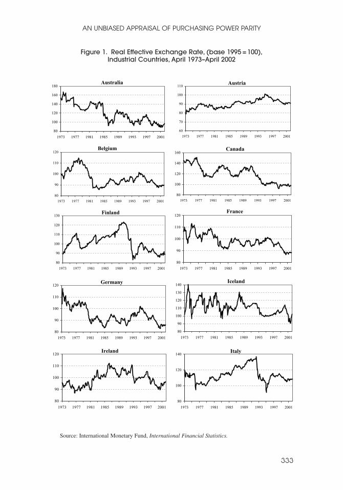
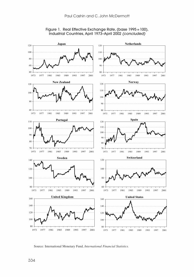
The REER data for all 20 countries are set out in Figure 1—an increase in theREER series indicates a real appreciation of the country’s currency.14 Several fea-tures of the data stand out. First, a cursory inspection of the REER series indicatesthat most countries have real exchange rates that appear to exhibit symptoms ofdrift or nonstationarity. There appear to be substantial and sustained deviationsfrom PPP (that is, nonstationarity in the REER). The evolution of REER appearsto be a highly persistent, slow-moving process; for most countries the REER doesnot appear to cycle about any particular equilibrium value, especially for Japan(the general appreciation of its exchange rate is typical of a process with a unit

qPRP Ri

i i

j jj i

Wij

=

≠∏ ,


332

13Wij can be interpreted as the sum over all markets of a gauge of the degree of competition betweenproducers of country i and j, divided by the sum over all markets of a gauge of the degree of competitionbetween producers of country i and all other producers.

14The 20 countries (and IFS country numbers) are Australia (193), Austria (122), Belgium (124),Canada (156), Finland (172), France (132), Germany (134), Iceland (176), Ireland (178), Italy (136),Japan (158), Netherlands (138), New Zealand (196), Norway (142), Portugal (182), Spain (184), Sweden(144), Switzerland (146), United Kingdom (112), and the United States (111). A decline (depreciation) ina country’s REER index indicates a rise in its international competitiveness (defined as the relative priceof domestic tradable goods in terms of foreign tradables). For a detailed explanation and critique of howthe IMF’s REER indices are constructed, see Zanello and Desruelle (1997) and Wickham (1993).


333

Australia

80

100

120

140

160

180

1973 1977 1981 1985 1989 1993 1997 2001

Belgium

80

90

100

110

120

1973 1977 1981 1985 1989 1993 1997 2001

Canada

80

100

120

140

160

1973 1977 1981 1985 1989 1993 1997 2001

Finland

80

90

100

110

120

130

1973 1977 1981 1985 1989 1993 1997 2001

France

80

90

100

110

120

1973 1977 1981 1985 1989 1993 1997 2001

Germany

80

90

100

110

120

1973 1977 1981 1985 1989 1993 1997 2001

Iceland

80

90

100

110

120

130

140

1973 1977 1981 1985 1989 1993 1997 2001

Ireland

80

90

100

110

120

1973 1977 1981 1985 1989 1993 1997 2001

Italy

80

100

120

140

1973 1977 1981 1985 1989 1993 1997 2001

Austria

60

70

80

90

100

110

1973 1977 1981 1985 1989 1993 1997 2001

Figure 1. Real Effective Exchange Rate, (base 1995 =100),Industrial Countries, April 1973–April 2002

Source: International Monetary Fund, International Financial Statistics.


334

Japan

40

60

80

100

120

1973 1977 1981 1985 1989 1993 1997 2001

Netherlands

80

90

100

110

120

1973 1977 1981 1985 1989 1993 1997 2001

New Zealand

60

80

100

120

1973 1977 1981 1985 1989 1993 1997 2001

Norway

80

90

100

110

120

1973 1977 1981 1985 1989 1993 1997 2001

Portugal

70

80

90

100

110

1973 1977 1981 1985 1989 1993 1997 2001

Spain

70

80

90

100

110

120

1973 1977 1981 1985 1989 1993 1997 2001

Sweden

80

100

120

140

1973 1977 1981 1985 1989 1993 1997 2001

Switzerland

60

80

100

120

1973 1977 1981 1985 1989 1993 1997 2001

United Kingdom

80

100

120

140

160

1973 1977 1981 1985 1989 1993 1997 2001

United States

80

100

120

140

160

1973 1977 1981 1985 1989 1993 1997 2001

Figure 1. Real Effective Exchange Rate, (base 1995 =100),Industrial Countries, April 1973–April 2002 (concluded)

Source: International Monetary Fund, International Financial Statistics.

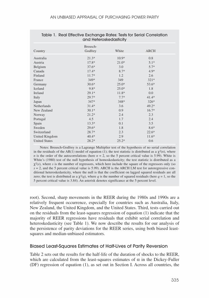
root). Second, sharp movements in the REER during the 1980s and 1990s are arelatively frequent occurrence, especially for countries such as Australia, Italy,New Zealand, the United Kingdom, and the United States. Third, tests carried outon the residuals from the least-squares regression of equation (1) indicate that themajority of REER regressions have residuals that exhibit serial correlation andheteroskedasticity (see Table 1). We now describe the results for our analysis ofthe persistence of parity deviations for the REER series, using both biased least-squares and median-unbiased estimators.

Biased Least-Squares Estimates of Half-Lives of Parity Reversion

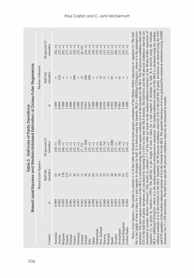
Table 2 sets out the results for the half-life of the duration of shocks to the REER,which are calculated from the least-squares estimates of α in the Dickey-Fuller(DF) regression of equation (1), as set out in Section I. Across all countries, the


335

Table 1. Real Effective Exchange Rates: Tests for Serial Correlationand Heteroskedasticity

Breusch-Country Godfrey White ARCH

Australia 21.3* 10.9* 0.8Austria 17.8* 21.0* 5.1*Belgium 37.6* 3.0 5.7*Canada 17.4* 8.7* 4.9*Finland 11.7* 1.2 2.6France 349* 349 321*Germany 30.6* 25.0* 53.6*Iceland 9.8* 25.0* 1.8Ireland 29.1* 11.8* 0.0Italy 29.7* 7.7* 41.4*Japan 347* 348* 326*Netherlands 31.4* 3.6 49.2*New Zealand 30.1* 0.9 16.7*Norway 21.2* 2.4 2.3Portugal 4.5 1.7 2.4Spain 13.3* 0.1 3.5Sweden 29.6* 1.8 8.6*Switzerland 28.7* 2.3 22.6*United Kingdom 40.4* 2.9 11.6*United States 28.2* 25.2* 0.6

Notes: Breusch-Godfrey is a Lagrange Multiplier test of the hypothesis of no serial correlationin the residuals of the AR(1) model of equation (1); the test statistic is distributed as a χ2(n), wheren is the order of the autocorrelations (here n = 2, so the 5 percent critical value is 5.99). White isWhite’s (1980) test of the null hypothesis of homoskedasticity; the test statistic is distributed as aχ2(s), where s is the number of regressors, which here include the square of the regressors only (sos = 2, and the 5 percent critical value is 5.99). ARCH is the ARCH LM test for autoregressive con-ditional heteroskedasticity, where the null is that the coefficient on lagged squared residuals are allzero; the test is distributed as a χ2(q), where q is the number of squared residuals (here q = 1, so the5 percent critical value is 3.84). An asterisk denotes significance at the 5 percent level.


336

Tab

le 2

.H

alf-

Live

s o

f Pa

rity

De

via

tion

s:

Bia

sed

Le

ast

-Sq

ua

res

an

d M

ed

ian

-Un

bia

sed

Est

ima

tion

of D

icke

y-Fu

ller

Reg

ress

ion

s

Bia

sed

Lea

st S

quar

esM

edia

n U

nbia

sed

——

——

——

——

——

——

——

——

——

——

——

——

——

——

——

——

——

——

——

——

——

——

Hal

f-lif

e 90

per

cent

CI

Hal

f-lif

e 90

per

cent

CI

Cou

ntry

α(m

onth

s)(m

onth

s)α

(mon

ths)

(mon

ths)

Aus

tral

ia0.

989

63[3

0,∞

]1.

000

∞[4

2,∞

]A

ustr

ia0.

982

38[2

3,10

4]0.

994

120

[25,

∞]

Bel

gium

0.99

513

8[4

6,∞

]1.

000

∞[9

2,∞

]C

anad

a 0.

994

115

[47,

∞]

1.00

0∞

[77,

∞]

Finl

and

0.99

177

[32,

∞]

1.00

0∞

[51,

∞]

Fran

ce0.

985

46[2

2,∞

]0.

998

300

[30,

∞]

Ger

man

y0.

987

53[2

5,∞

]1.

000

∞[3

5,∞

]Ic

elan

d0.

941

11[7

,23]

0.94

913

[8,4

2]Ir

elan

d0.

981

36[1

9,34

0]0.

993

100

[24,

∞]

Ital

y0.

984

43[2

2,∞

]0.

997

200

[29,

∞]

Japa

n0.

990

69[3

3,∞

]1.

000

∞[4

6,∞

]N

ethe

rlan

ds0.

987

53[2

5,∞

]1.

000

∞[3

5,∞

]N

ew Z

eala

nd0.

971

24[1

4,84

]0.

980

35[1

6,∞

]N

orw

ay0.

969

22[1

3,74

]0.

978

31[1

5,∞

]Po

rtug

al0.

991

77[3

2,∞

]1.

000

∞[5

1,∞

]Sp

ain

0.98

340

[22,

200]

0.99

393

[27,

∞]

Swed

en0.

993

99[3

7,∞

]1.

000

∞[6

6,∞

]Sw

itzer

land

0.97

426

[16,

76]

0.98

341

[17,

∞]

Uni

ted

Kin

gdom

0.98

963

[27,

∞]

1.00

0∞

[42,

∞]

Uni

ted

Stat

es0.

994

115

[38,

∞]

1.00

0∞

[77,

∞]

Not

es:L

east

Squ

ares

—T

he r

esul

ts in

col

umns

2–

4 of

this

tabl

e ar

e ba

sed

on le

ast-

squa

res

estim

atio

n of

the

Dic

key-

Fulle

r re

gres

sion

of

equa

tion

(1).

The

hal

f-lif

e is

the

len

gth

of t

ime

it ta

kes

for

a un

it im

puls

e to

dis

sipa

te b

y ha

lf. I

t is

der

ived

usi

ng t

he f

orm

ula:

HL

S =

AB

S(lo

g(1/

2)/lo

g(α)

),w

here

αis

the

aut

oreg

ress

ive

para

met

er. T

he le

ast-

squa

res

estim

ate

of th

e H

LS

is c

alcu

late

d us

ing

the

leas

t-sq

uare

s es

timat

e of

αin

the

form

ula

for

the

HL

S. T

he 9

0 pe

rcen

t con

fide

nce

inte

rval

s(C

I) o

f th

e ha

lf-l

ife

of p

arity

dev

iatio

ns a

re c

alcu

late

d by

inse

rtin

g α̂

±1.

65×

se (

α̂)

into

the

HL

S fo

rmul

a. T

he h

alf-

lives

and

the

90 p

erce

nt c

onfi

denc

e in

terv

als

are

mea

sure

d in

mon

ths.

Med

ian

Unb

iase

d—

The

res

ults

in

colu

mns

5–7

of

this

tab

le a

re b

ased

on

the

med

ian-

unbi

ased

est

imat

es o

f th

e D

icke

y-Fu

ller

regr

essi

on o

feq

uatio

n (1

),as

giv

en b

y A

ndre

ws

(199

3).

The

hal

f-lif

e is

the

len

gth

of t

ime

it ta

kes

for

a un

it im

puls

e to

dis

sipa

te b

y ha

lf.

It i

s de

rive

d us

ing

the

form

ula:

HL

S =

AB

S(lo

g(1/

2)/lo

g(α)

),w

here

αis

the

med

ian-

unbi

ased

aut

oreg

ress

ive

para

met

er. T

he m

edia

n-un

bias

ed e

stim

ate

of t

he H

LS

is c

alcu

late

d us

ing

the

med

ian-

unbi

ased

est

imat

e of

αin

the

for

mul

a fo

r th

e H

LS.

Sim

ilarl

y,th

e 90

per

cent

con

fide

nce

inte

rval

s (C

I) o

f th

e ha

lf-l

ife

of p

arity

dev

iatio

ns a

re d

eriv

ed u

sing

the

0.0

5an

d 0.

95 q

uant

iles

of th

e m

edia

n-un

bias

ed e

stim

ate

of α̂

in th

e fo

rmul

a fo

r the

HL

S. T

he q

uant

ile fu

nctio

ns o

f α̂w

ere

gene

rate

d by

num

eric

al s

imul

atio

n (u

sing

10,

000

itera

tions

) fo

r T

= 34

9 ob

serv

atio

ns. T

he h

alf-

lives

and

the

90 p

erce

nt c

onfi

denc

e in

terv

als

are

mea

sure

d in

mon

ths.

mean half-life of parity reversion is 60 months and the median half-life is 53months.15 This result is consistent with Rogoff’s (1996) consensus of half-lives ofparity reversion of between 36 to 60 months (three to five years).

We also report 90 percent confidence intervals for the least-squares half-life ofPPP deviations, in order to gauge the variability of the persistence of shocks to thereal exchange rate. The confidence intervals are quite wide and encompass half-lives that are consistent with both PPP holding and not holding in the long run.This indicates that there is a high level of uncertainty about the “true” value of thehalf-life of PPP deviations. For seven countries the upper bound of the 90 percentconfidence interval is finite, indicating that these countries have finitely persistentshocks to their real exchange rates. It is important to note that the confidence inter-vals used here are formed assuming that the estimated autoregressive parameterhas a t-distribution, which we know to be incorrect, and further biases hypothesistests toward rejecting the unit root null.

As an example of how to interpret the table, we take the particular cases ofIceland and Canada. For Iceland, the least-squares (LS) estimate of α is 0.941.Moreover, the time it takes for half of the shock to the REER of Iceland to dissi-pate is 11 months, while the length of the 90 percent confidence interval for theLS estimate of the half-life of deviations from parity is 7 to 23 months.Accordingly, shocks to the REER of Iceland do not appear to be very persistent,at least relative to the persistence found in other countries’ real exchange rates.

For Canada, the LS estimate of α is 0.994. Moreover, the time it takes for halfof the shock to Canada’s REER to dissipate is 115 months, while the length of the90 percent confidence interval for the LS estimate of the half-life of deviationsfrom parity is 47 to ∞ months. Accordingly, shocks to the REER of Canada doappear to be very persistent, especially since the lower bound of the 90 percentconfidence interval indicates that there is only a 5 percent chance that the true half-life of parity reversion of the REER is shorter than 47 months.

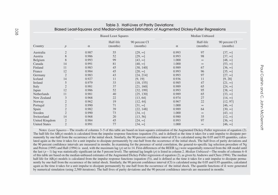
The DF regression results presented in Table 2 do not attempt to account forthe presence of serial correlation. Tests for serial correlation carried out on theresiduals from the least-squares regression of equation (1) indicate that all REERregressions (except Portugal) have residuals with serial correlation (see column 2of Table 1). Accordingly, least-squares estimates of the Augmented Dickey-Fuller(ADF) regressions, which do account for serial correlation, are set out in Table 3.In examining for the presence of serial correlation, the general-to-specific lagselection procedure of Ng and Perron (1995) and Hall (1994) is used, with themaximum lag set to 14.16 For all countries at least one lag (p = 2) of the first dif-ference of the REER is significant, which ensures that the ADF half-lives will dif-fer from the DF half-lives. The ADF half-lives are typically shorter in durationthan those derived from the DF regression, ranging from 11 months (Iceland) to


337

15These half-life results are comparable to those obtained by Cheung and Lai (2000b) using least-squares estimation on monthly bilateral (post–Bretton Woods) dollar real exchange rates, which calculatedan average half-life of 3.3 years.

16Starting with the maximum lag, first-differences of the logarithm of the REER (qt) were sequentiallyremoved from the AR model until the last lag was statistically significant (at the 5 percent level). At thatpoint all lag lengths smaller than or equal to p – 1 are included in the AR(p) regression of equation (2).

Pau

l Ca

shin

an

d C

.Joh

n M

cD

erm

ott

33

8

Table 3. Half-Lives of Parity Deviations: Biased Least-Squares and Median-Unbiased Estimation of Augmented Dickey-Fuller Regressions

Biased Least Squares Median Unbiased———————————————————— ————————————————————

Half-life 90 percent CI Half-life 90 percent CICountry p α (months) (months) α (months) (months)

Australia 2 0.987 55 [29, ∞] 0.993 97 [37, ∞]Austria 8 0.986 52 [29, ∞] 0.993 98 [37, ∞]Belgium 8 0.993 99 [43, ∞] 1.000 ∞ [48, ∞]Canada 14 0.991 81 [40, ∞] 1.000 ∞ [53, ∞]Finland 11 0.983 45 [30, 140] 0.989 67 [36, ∞]France 12 0.984 45 [20, ∞] 0.993 96 [35, ∞]Germany 2 0.983 43 [24, 214] 0.993 97 [27, ∞]Iceland 14 0.927 11 [9, 19] 0.936 11 [9, 28]Ireland 5 0.979 33 [18, 155] 0.985 47 [21, ∞]Italy 2 0.981 37 [21, 160] 0.989 65 [24, ∞]Japan 12 0.986 52 [32, 199] 0.993 95 [38, ∞]Netherlands 11 0.981 40 [25, 130] 0.989 65 [33, ∞]New Zealand 3 0.968 22 [13, 64] 0.974 27 [14, ∞]Norway 2 0.962 19 [12, 44] 0.967 22 [12, 97]Portugal 2 0.990 71 [31, ∞] 1.000 ∞ [46, ∞]Spain 2 0.982 39 [22, 148] 0.989 64 [30, ∞]Sweden 2 0.990 73 [34, ∞] 1.000 ∞ [43, ∞]Switzerland 14 0.968 20 [13, 56] 0.980 35 [12, ∞]United Kingdom 2 0.984 45 [24, ∞] 0.993 97 [36, ∞]United States 2 0.991 77 [34, ∞] 1.000 ∞ [46, ∞]

Notes: Least Squares—The results of columns 3–5 of this table are based on least-squares estimation of the Augmented Dickey-Fuller regression of equation (2).The half-life for AR(p) models is calculated from the impulse response functions (equation (5)), and is defined as the time it takes for a unit impulse to dissipate per-manently by one-half from the occurrence of the initial shock. Similarly, the 90 percent confidence interval (CI) is calculated using the 0.05 and 0.95 quantiles, calcu-lated again as the time it takes for a unit impulse to dissipate permanently by one-half from the occurrence of the initial shock. The half-lives of parity deviations andthe 90 percent confidence intervals are measured in months. In examining for the presence of serial correlation, the general-to-specific lag selection procedure of Ngand Perron (1995) and Hall (1994) is used, with the maximum lag (p) set to 14. First-differences of the REER (qt) were sequentially removed from the AR model untilthe last (p – 1) lag was statistically significant (at the 5 percent level). The optimal lag length (p) is listed in column 2. Median Unbiased—The results of columns 6–8of this table are based on the median-unbiased estimates of the Augmented Dickey-Fuller regression of equation (2), as given by Andrews and Chen (1994). The medianhalf-life for AR(p) models is calculated from the impulse response functions (equation (5)), and is defined as the time it takes for a unit impulse to dissipate perma-nently by one-half from the occurrence of the initial shock. Similarly, the 90 percent confidence interval (CI) is calculated using the 0.05 and 0.95 quantiles, calculatedagain as the time it takes for a unit impulse to dissipate permanently by one-half from the occurrence of the initial shock. The quantile functions of α̂ were generatedby numerical simulation (using 2,500 iterations). The half-lives of parity deviations and the 90 percent confidence intervals are measured in months.

99 months (Belgium). Across all countries, the mean half-life of parity reversionis 48 months and the median half-life is 45 months. While for several countries the90 percent confidence interval is narrower than for the DF regression (such as NewZealand and Norway), in several cases the variability of shocks to the REER is sowide as to include infinity as the upper bound of the confidence interval (such asCanada and the United States).17

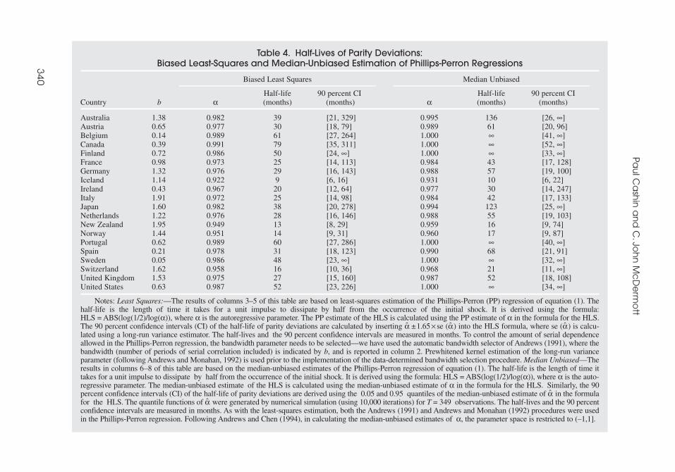
The ADF regressions presented in Table 3 do not attempt to account for thepresence of heteroskedasticity, and so will be invalid when there are departuresfrom the maintained hypothesis of AR(p) errors. Tests for heteroskedasticity car-ried out on the residuals from the least-squares regression of equation (1) indicatethat most REER regressions have residuals with heteroskedasticity (see columns3–4 of Table 1). Accordingly, given the presence of heteroskedasticity and serialcorrelation (including moving-average error structures) in the real exchange rateseries, the results of Phillips-Perron (PP) regressions, which are valid in the pres-ence of serial correlation and heteroskedasticity, are presented in Table 4. Theduration of PP half-lives are typically lower again than those derived from theADF and DF regressions, ranging from 9 months (Iceland) to 79 months (Canada).Across all countries, the mean half-life of parity reversion from the PP regressionis 35 months and the median half-life is 30 months. For those countries with finiteupper bounds for the 90 percent confidence interval of the half-lives of deviationsfrom parity, the confidence intervals based on PP regressions are typically tighterthan those derived from the ADF and DF regressions, yet continue to encompassa wide range of half-lives. Controlling for the serial correlation present in the datalowers considerably the estimated half-life of parity deviations—the PP regres-sions detect more serial correlation than the ADF and DF regressions, and thusproduce lower estimated half-lives of deviations from parity.

Broadly, the three least-squares results of Tables 2–4 indicate that across allcountries the median half-life of parity deviations is finite, with an average lengthof about four years, and a lower bound on the confidence intervals for the truehalf-lives of about two years. However, the upper bound of the confidence inter-val for many REER is greater than ten years (and in many cases is infinity).

Median-Unbiased Estimates of Half-Lives of Parity Reversion

The half-lives of PPP deviations calculated above (using the least-squares esti-mator) are reasonably close to Rogoff’s (1996) consensus of three to five years(36 to 60 months). However, as noted in Section I above, the least-squares esti-mator of the autoregressive parameter in each of the DF, ADF, and PP regres-sions is biased downward. As a result, the above calculations of the duration of deviations from PPP are also likely to be biased downward (and in favor offinding that PPP holds in the REER data). Consequently, we remove this bias by


339

17Consistent with Papell (1997), we find that accounting for serial correlation in the disturbancesweakens the evidence against a null hypothesis of a unit root in the real exchange rate series, as thepoint estimates of the autoregressive parameter are typically lower in the AR(p) case than for the AR(1)regression.

Pau

l Ca

shin

an

d C

.Joh

n M

cD

erm

ott

34

0

Table 4. Half-Lives of Parity Deviations: Biased Least-Squares and Median-Unbiased Estimation of Phillips-Perron Regressions

Biased Least Squares Median Unbiased———————————————————— ————————————————————

Half-life 90 percent CI Half-life 90 percent CICountry b α (months) (months) α (months) (months)

Australia 1.38 0.982 39 [21, 329] 0.995 136 [26, ∞]Austria 0.65 0.977 30 [18, 79] 0.989 61 [20, 96]Belgium 0.14 0.989 61 [27, 264] 1.000 ∞ [41, ∞]Canada 0.39 0.991 79 [35, 311] 1.000 ∞ [52, ∞]Finland 0.72 0.986 50 [24, ∞] 1.000 ∞ [33, ∞]France 0.98 0.973 25 [14, 113] 0.984 43 [17, 128]Germany 1.32 0.976 29 [16, 143] 0.988 57 [19, 100]Iceland 1.14 0.922 9 [6, 16] 0.931 10 [6, 22]Ireland 0.43 0.967 20 [12, 64] 0.977 30 [14, 247]Italy 1.91 0.972 25 [14, 98] 0.984 42 [17, 133]Japan 1.60 0.982 38 [20, 278] 0.994 123 [25, ∞]Netherlands 1.22 0.976 28 [16, 146] 0.988 55 [19, 103]New Zealand 1.95 0.949 13 [8, 29] 0.959 16 [9, 74]Norway 1.44 0.951 14 [9, 31] 0.960 17 [9, 87]Portugal 0.62 0.989 60 [27, 286] 1.000 ∞ [40, ∞]Spain 0.21 0.978 31 [18, 123] 0.990 68 [21, 91]Sweden 0.05 0.986 48 [23, ∞] 1.000 ∞ [32, ∞]Switzerland 1.62 0.958 16 [10, 36] 0.968 21 [11, ∞]United Kingdom 1.53 0.975 27 [15, 160] 0.987 52 [18, 108]United States 0.63 0.987 52 [23, 226] 1.000 ∞ [34, ∞]

Notes: Least Squares:—The results of columns 3–5 of this table are based on least-squares estimation of the Phillips-Perron (PP) regression of equation (1). Thehalf-life is the length of time it takes for a unit impulse to dissipate by half from the occurrence of the initial shock. It is derived using the formula:HLS = ABS(log(1/2)/log(α)), where α is the autoregressive parameter. The PP estimate of the HLS is calculated using the PP estimate of α in the formula for the HLS.The 90 percent confidence intervals (CI) of the half-life of parity deviations are calculated by inserting α̂ ±1.65 × se (α̂) into the HLS formula, where se (α̂) is calcu-lated using a long-run variance estimator. The half-lives and the 90 percent confidence intervals are measured in months. To control the amount of serial dependenceallowed in the Phillips-Perron regression, the bandwidth parameter needs to be selected—we have used the automatic bandwidth selector of Andrews (1991), where thebandwidth (number of periods of serial correlation included) is indicated by b, and is reported in column 2. Prewhitened kernel estimation of the long-run varianceparameter (following Andrews and Monahan, 1992) is used prior to the implementation of the data-determined bandwidth selection procedure. Median Unbiased—Theresults in columns 6–8 of this table are based on the median-unbiased estimates of the Phillips-Perron regression of equation (1). The half-life is the length of time ittakes for a unit impulse to dissipate by half from the occurrence of the initial shock. It is derived using the formula: HLS = ABS(log(1/2)/log(α)), where α is the auto-regressive parameter. The median-unbiased estimate of the HLS is calculated using the median-unbiased estimate of α in the formula for the HLS. Similarly, the 90percent confidence intervals (CI) of the half-life of parity deviations are derived using the 0.05 and 0.95 quantiles of the median-unbiased estimate of α̂ in the formulafor the HLS. The quantile functions of α̂ were generated by numerical simulation (using 10,000 iterations) for T = 349 observations. The half-lives and the 90 percentconfidence intervals are measured in months. As with the least-squares estimation, both the Andrews (1991) and Andrews and Monahan (1992) procedures were usedin the Phillips-Perron regression. Following Andrews and Chen (1994), in calculating the median-unbiased estimates of α, the parameter space is restricted to (–1,1].

calculating median-unbiased point estimates and confidence intervals for theautoregressive parameter in equations (1) and (2).18

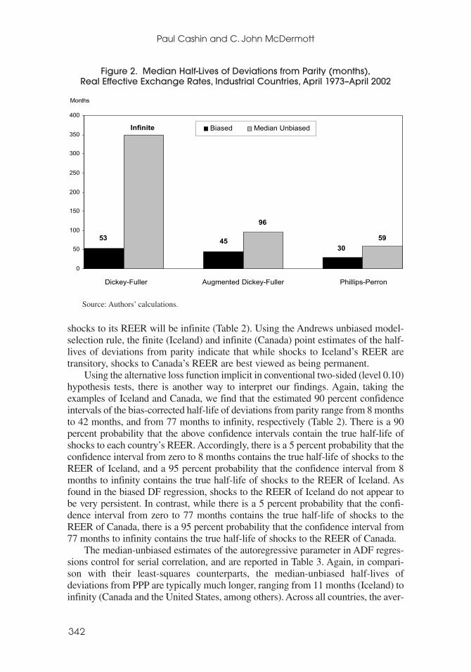
Median-unbiased estimates of the half-life of PPP deviations for the DF regres-sions are set out in Table 2. In comparison with the median-unbiased estimates ofα in DF regressions, the least-squares estimates of α are biased downward bybetween 0.005 and 0.013. While this is a small difference in absolute terms, it hasimportant implications for the half-life measures of the persistence of the REER.The median-unbiased point estimates of the half-lives are much greater than theirleast-squares counterparts for every country, with 11 of the countries having a half-life of infinity. Across all countries, the average (median) bias-corrected half-life ofparity reversion is infinity, clearly exceeding the average downwardly biased least-squares AR(1) half-life of 53 months (Figure 2). This implies no parity reversion,rather than the 15 percent per year calculated using biased DF methods. In addi-tion, the 90 percent confidence intervals for the median-unbiased estimates of half-lives of parity reversion are typically much wider than for their LS counterparts,and the REER of all countries in Table 2 (except Iceland) have an upper bound tothe confidence interval of the unbiased half-lives that embrace infinity.19

The results in Table 2 indicate that, using the Andrews unbiased model-selectionrule, 9 of the countries are subject to REER shocks that are finitely persistent, while11 of the countries experience permanent shocks to their REER series. The inter-pretation of this rule is that for any given country there is a 50 percent probabilitythat the confidence interval from zero to the estimated median-unbiased half-lifecontains the true half-life of shocks to its REER, and a 50 percent probability thatthe confidence interval from the estimated median-unbiased half-life to infinitycontains the true half-life of shocks to its REER. Let us again take the examples ofIceland (short-lived half-life) and Canada (infinite half-life). While there is a 50percent probability that the confidence interval from zero to 13 months contains thetrue half-life of shocks to the REER of Iceland, there is also a 50 percent probabil-ity that the confidence interval from 13 months to infinity contains the true half-lifeof shocks to the REER of Iceland. For Canada, while there is a 50 percent proba-bility that the confidence interval with a finite upper bound contains the true half-life of shocks to its REER, there is a 50 percent probability that the true half-life of


341

18Median-unbiased estimates (and confidence intervals) of the half-life of a shock (for T = 349 obser-vations (1973:4–2002:4)) were determined using quantile functions of α̂ generated by: numerical simula-tion (using 10,000 iterations), following the method suggested by Appendix B of Andrews (1993) for theDF regression of equation (1) (see Table 2); numerical simulation (using 10,000 iterations), following themethod suggested by McDermott (1996) for the PP regression of equation (1) (see Table 4); and numeri-cal simulation (using 2,500 iterations), following the method suggested by Andrews and Chen (1994) forthe ADF regression of equation (2) (see Table 3).

19Our results for the median-unbiased Dickey-Fuller regression are similar to those of Andrews (1993),who calculated point and interval estimates of the half-life of monthly bilateral dollar real exchange rates forseveral industrial countries over the period 1973 to 1988. He found that, using least squares, the half-life ofPPP deviations for each real exchange rate was finite, with an average half-life of about 31 months. However,using the median-unbiased procedure (for an AR(1) model) only three of the eight real exchange rates hadfinite half-lives of PPP deviations, with an average half-life of about 60 months. The remaining five exhib-ited permanent parity deviations. Similarly, while all of Andrews’ median-unbiased lower bounds of the 90percent confidence interval were less than 36 months (as is the case for the majority of countries in the pre-sent study), the upper bounds were all infinite (as is the case for all but one country in the present study).

shocks to its REER will be infinite (Table 2). Using the Andrews unbiased model-selection rule, the finite (Iceland) and infinite (Canada) point estimates of the half-lives of deviations from parity indicate that while shocks to Iceland’s REER aretransitory, shocks to Canada’s REER are best viewed as being permanent.

Using the alternative loss function implicit in conventional two-sided (level 0.10)hypothesis tests, there is another way to interpret our findings. Again, taking theexamples of Iceland and Canada, we find that the estimated 90 percent confidenceintervals of the bias-corrected half-life of deviations from parity range from 8 monthsto 42 months, and from 77 months to infinity, respectively (Table 2). There is a 90percent probability that the above confidence intervals contain the true half-life ofshocks to each country’s REER. Accordingly, there is a 5 percent probability that theconfidence interval from zero to 8 months contains the true half-life of shocks to theREER of Iceland, and a 95 percent probability that the confidence interval from 8months to infinity contains the true half-life of shocks to the REER of Iceland. Asfound in the biased DF regression, shocks to the REER of Iceland do not appear tobe very persistent. In contrast, while there is a 5 percent probability that the confi-dence interval from zero to 77 months contains the true half-life of shocks to theREER of Canada, there is a 95 percent probability that the confidence interval from77 months to infinity contains the true half-life of shocks to the REER of Canada.

The median-unbiased estimates of the autoregressive parameter in ADF regres-sions control for serial correlation, and are reported in Table 3. Again, in compari-son with their least-squares counterparts, the median-unbiased half-lives ofdeviations from PPP are typically much longer, ranging from 11 months (Iceland) toinfinity (Canada and the United States, among others). Across all countries, the aver-


342

0

50

100

150

200

250

300

350

400

Biased Median Unbiased

Dickey-Fuller Augmented Dickey-Fuller Phillips-Perron

Infinite

53

96

4530

59

Months

Figure 2. Median Half-Lives of Deviations from Parity (months),Real Effective Exchange Rates, Industrial Countries, April 1973–April 2002

Source: Authors’ calculations.

age bias-corrected half-life of parity reversion is 96 months, in excess of the averagedownwardly biased least-squares AR(p) half-life of 45 months (Figure 2). Thisimplies a rate of parity reversion of only 8 percent per year, rather than the 17 per-cent per year calculated using biased ADF methods. Similarly, the median-unbiasedconfidence intervals are much wider than their least-squares counterparts. TheAndrews unbiased model-selection rule indicates that all but 5 of the 20 countrieshave finitely persistent shocks to their REER, which is consistent with the reversionof REER to parity. However of all 20 countries, only Iceland and Norway produceda 90 percent confidence interval for the unbiased half-life of deviations from paritythat did not include infinity. Taking the United Kingdom as an example, while thereis a 50 percent probability that the confidence interval from zero to 97 months con-tains the true half-life of shocks to its REER, there is also a 50 percent probabilitythat the confidence interval from 97 months to infinity contains the true half-life. Inaddition, while there is a 5 percent probability that the confidence interval from zeroto 36 months contains the true half-life of shocks to the REER of the UnitedKingdom, there is a 95 percent probability that the confidence interval from 36months to infinity contains the true half-life (Table 3). The width of this confidenceinterval for the half-life indicates there is a great deal of uncertainty as to the dura-tion of the true half-life of parity reversion of the United Kingdom’s REER.

Our bias-corrected ADF regression results accord with those obtained byMurray and Papell (2000), who follow Andrews and Chen (1994) in calculatingmedian-unbiased estimates of half-lives for bilateral dollar real exchange rates.They find that the average bias-corrected half-life is about three years, but with con-fidence intervals that are typically so large that the point estimates of bias-correctedhalf-lives from ADF regressions provide virtually no information regarding thetrue size of the half-lives. However, an important deficiency of the Murray-Papellanalysis is the inability of their ADF bias-correction method to account for time-dependent heteroskedasticity, which is a common feature of real exchange rateseries. Once allowance is made for a wider class of serial correlation and het-eroskedasticity, as is done in this paper, the speed of parity reversion is typicallyfaster than that found with other median-unbiased models (see Figure 2).

The regression that corrects for the least-squares downward bias, and controlsfor serial correlation and heteroskedasticity, is the median-unbiased PP regression,the results of which are reported in Table 4. Across all countries, the average bias-corrected half-life of parity reversion is 59 months, clearly exceeding the averagedownwardly biased least-squares PP half-life of 30 months (see Figure 2). Thisimplies a rate of parity reversion of only 13 percent per year, rather than the 24percent per year calculated using biased PP methods. The broad pattern found inthe biased least-squares estimates of half-lives of parity reversion is also found forthe median-unbiased estimates of half-lives of parity reversion, with the estima-tion method that controls for serial correlation and heteroskedasticity (the PPregression) clearly yielding the smallest half-lives of deviations from parity.20


343

20In the context of biased least-squares estimation, Lothian and Taylor (2000) also find much smallerestimates of the half-lives of shocks to the dollar-sterling real exchange rate when using heteroskedastic-ity-robust PP regressions rather than ADF regressions.

As shown in Figure 2, implementation of methods of bias correction that donot account for both the serial correlation and heteroskedasticity present in realexchange rate data will tend to overestimate the duration of the half-life of devia-tions from parity, and erroneously indicate that purchasing power parity does nothold in the post–Bretton Woods period. Interestingly, the average half-life of par-ity deviations derived from median-unbiased PP methods is very close to the aver-age half-life of parity deviations derived from (conventional) biased DF estimationmethods.21 However, the downwardly biased least-squares DF estimates of thehalf-lives of deviations from parity yield no cases of infinite half-lives; in contrast,6 of the 20 countries experience non-finite half-lives using bias-corrected PP esti-mation methods (see Tables 2 and 4).

While the cross-country average half-lives of parity reversion based on themedian-unbiased PP regression are slightly longer than the cross-country averagebased on the biased least-squares DF regression (see Figure 2), the country-specificresults display quite a deal of heterogeneity. For those countries that have relativelysmall (biased) DF estimates of the autoregressive parameter (such as Iceland), thebias-corrected PP estimates of the autoregressive parameter tend to be lower thanthe biased DF estimates—this is consistent with faster speeds of parity reversionand greater evidence in favor of purchasing power parity (see Figure 3). In contrast,for those countries that have relatively large (biased) DF estimates of the autore-gressive parameter (such as Australia), the bias-corrected PP estimates of theautoregressive parameter tend to be greater than the biased DF estimates.

Using the bias-corrected PP regression results, the Andrews unbiased model-selection rule indicates that all but 6 of the 20 countries have finitely persistentshocks to their REER, which is consistent with the reversion of REER to parity(Table 4). For example, the United Kingdom exhibits a median-unbiased half-life ofdeviation from parity of 52 months. Using the Andrews unbiased model-selectionrule, this indicates that the United Kingdom experiences finitely persistent (transi-tory) shocks to its REER. However, nine countries have 90 percent confidence inter-vals for their half-lives of deviations from parity that embrace infinity. Taking theUnited States as an example, while there is a 5 percent probability that the confidenceinterval from zero to 34 months contains the true half-life of shocks to its REER,there is a 95 percent probability that the confidence interval from 34 months to infin-ity contains the true half-life (Table 4). Using the Andrews unbiased model-selectionrule, the unit root model is the most appropriate representation of the United StatesREER, and so shocks to its REER are best viewed as being permanent.22


344

21The presence of moving average and heteroskedastic errors in the real exchange rate data (as set out inTable 1) is most likely attributable to outliers in the real exchange rate data. The Phillips-Perron regressioncontrols for this form of heteroskedasticity, while the Augmented Dickey-Fuller and Dickey-Fuller regressionsdo not. As a result, estimated half-lives calculated from the latter two models (derived from both biased least-squares and median-unbiased estimators) will be greater than those derived from the biased and bias-correctedPhillips-Perron model. In addition, the Phillips-Perron regression picks up more serial correlation (particularlyof the moving average type), which would also reduce the estimated half-lives of parity deviations.

22As a check of the robustness of our results, for the same sample of countries as studied in this paper,McDermott (1996) found that (using the bias-corrected Phillips-Perron method) the persistence propertiesof shocks to the real effective and real bilateral exchange rate series were very similar. In addition, a com-parison of the two versions of the real exchange rate for Canada, Japan, and the United Kingdom (usingthe bias-corrected Dickey-Fuller method) again found that the median-unbiased persistence results for realbilateral exchange rates are very similar to those derived using the real effective exchange rate series.

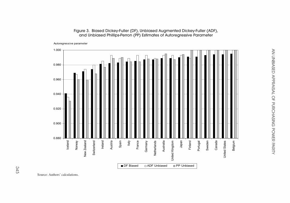
AN

UN

BIASED

AP

PR

AISA

L OF P

UR

CH

ASIN

G P

OW

ER PA

RITY

34

5

0.880

0.900

0.920

0.940

0.960

0.980

1.000

Icel

and

Nor

way

New

Zea

land

Sw

itzer

land

Irela

nd

Aus

tria

Spa

in

Italy

Fran

ce

Ger

man

y

Net

herla

nds

Aus

tralia

Uni

ted

Kin

gdom

Japa

n

Finl

and

Por

tuga

l

Sw

eden

Can

ada

Uni

ted

Sta

tes

Bel

gium

DF Biased ADF Unbiased PP Unbiased

Autoregressive parameter

Figure 3. Biased Dickey-Fuller (DF), Unbiased Augmented Dickey-Fuller (ADF),and Unbiased Phillips-Perron (PP) Estimates of Autoregressive Parameter

Source: Authors’ calculations.

For the majority of countries, these typically finite half-lives of deviationsfrom parity, and associated slow speeds of parity reversion, are consistent with thefindings of Flood and Taylor (1996). They find that evidence in favor of PPP ishard to discern from analyses of the short-run behavior of real exchange rates.However, once the data are averaged over 10 and 20 years, the regression coeffi-cient (in a pooled regression of the exchange rate change on the inflation differ-ential averages) is statistically significant and close to unity, providing strongerevidence of PPP.

In contrast to the above results, Taylor (2001) argues that there are two sourcesof upward bias in the conventional estimation of the speed of parity reversion:first, temporal aggregation bias, whereby sampling data at low frequencies doesnot allow one to identify a high-frequency adjustment process; and second, the lin-ear AR(1) specification of the standard (Dickey-Fuller) unit root model, whichassumes that reversion occurs monotonically, regardless of how far the process isfrom parity. However, as the present paper uses monthly REER data, the temporalaggregation bias is likely to be minimal. In addition, our use of AR(p) modelsallows for shocks to the REER to decline at a rate that is not necessarily constant.23

Taylor finds that when both sources of upward bias are present, then the estimatedhalf-life can be between 1.5 to 2.2 times the true half-life, for the case whenmonthly averaged data are being used to estimate a monthly (or greater) half-lifenonlinear threshold autoregressive process. Taylor (2001, p. 491) also acknowl-edges that month-to-month variation in nominal exchange rates is likely to dwarfthe variation in prices, and that the former are accurately measured in theInternational Monetary Fund’s IFS data. In comparison, the results from Tables 3and 4 indicate that even after controlling for serial correlation and heteroskedas-ticity, the bias-corrected half-life of parity deviations is typically about twice aslarge as the downwardly biased half-life.24

III. Conclusion

This paper has reexamined whether purchasing power parity (PPP) holds duringthe post–Bretton Woods period, by investigating the time-series properties of thereal effective exchange rate for 20 industrial countries. The theory of relative PPPholds that the exchange rate will be proportional to the ratio of money price levels(including traded and nontraded goods) between countries, which implies that


346

23While median-unbiased estimation allowing for AR(p) behavior does engender a non-monotonicimpulse response function, the shape of that impulse response function will be unaffected by the size ofthe shock to the real exchange rate. In contrast, methods that are robust to nonlinear adjustment to equi-librium allow for such an effect, yet do not correct for downwardly biased autoregressive parameters (seeTaylor, Peel, and Sarno, 2001, for a discussion of these issues).

24In addition to temporal aggregation bias, Imbs and others (2002) demonstrate that cross-sectionalaggregation bias raises the persistence of conventionally measured real exchange rate shocks. Cross-sectional aggregation bias arises from the failure of conventional estimation of the speed of parity rever-sion to take account of cross-sectoral heterogeneity in the dynamic properties of the typical componentsof aggregate price indices. This failure to allow for the persistence of relative prices to vary across sectorsinduces an upward bias in aggregate half-life measures, with the bias rising with the extent of cross-sectoral heterogeneity in the speed of parity reversion.

changes in relative price levels will be offset by changes in the exchange rate. Inassessing whether real exchange rates do converge to their equilibrium relativePPP value in the long run, we eschew undertaking hypothesis tests of whether realexchange rates follow a unit root process. Instead, we follow Andrews (1993) anduse point and interval statistics of the half-life of deviations from parity as our pre-ferred measure of the persistence of real exchange rate shocks.

Univariate studies of the hypothesis of unit roots in real exchange rates haveyielded consensus point estimates of the half-life of deviations of real exchangerates from purchasing power parity of between three to five years (Rogoff, 1996).Using conventional (least-squares) biased estimation of unit root models, we repli-cate the consensus finding in the literature. However, using median-unbiased esti-mation techniques that are robust to the presence of serial correlation and removethe downward bias of standard estimators, we find that the half-lives of parityreversion are longer than the consensus point estimate, with the cross-countryaverage of unbiased half-lives of deviations from parity lasting about eight years.

We concentrate on the results derived from the regression that allows for thebroadest error structure—median-unbiased estimates of Phillips-Perron regres-sions that are robust to the serial correlation and heteroskedasticity commonlyfound in real exchange rate series. In the post–Bretton Woods period, the majorityof countries are found to have finitely persistent shocks to their real effectiveexchange rates, which is consistent with the reversion of exchange rate deviationsfrom PPP. Averaging across all countries, the point estimate of the half-life of par-ity deviations is about five years, which is consistent with (but at the upper end of)Rogoff’s (1996) consensus estimate of the half-life of deviations from purchasingpower parity. In summary, while median-unbiased methods increase the estimatedhalf-life of deviations from PPP in comparison with downwardly biased least-squares-based methods, allowing for heteroskedasticity reduces the bias-correctedestimated half-life of parity deviations.

Using conventional two-sided hypothesis tests, the confidence interval of thebias-corrected half-life of deviations from parity is typically extremely wide,indicating that there is a great deal of uncertainty as to the “true” speed of parityreversion. When using the results from the heteroskedasticity-robust Phillips-Perron regression, 11 of the 20 countries in our sample have finite upper boundsto the confidence intervals of their half-lives of parity deviation, indicating thatfor just under half the countries the associated confidence intervals around thehalf-lives are too wide to provide much information as to whether PPP holds inthe long run. Although the null hypothesis of no PPP is not rejected at the 5 per-cent level for 9 of the 20 countries (as the upper bound of the bias-corrected con-fidence interval for the half-life contains infinity), failure to reject the nullhypothesis conveys little information as to the validity of PPP, as such a failuremay occur either because PPP is true, or because there is too much uncertainty asto the speed of reversion to PPP.

In contrast, using the median-unbiased point estimates of the half-lives ofdeviations from parity and the Andrews (1993) unbiased model-selection rule, wecan be more definitive about our willingness to draw conclusions as to the pres-ence or absence of parity reversion of real exchange rates in the post–Bretton


347

Woods period. When using the results from the heteroskedasticity-robust Phillips-Perron regression, we find that 14 of the 20 countries in our sample have finitebias-corrected half-lives of parity reversion. This indicates that for these countriesthere is a better than even chance that shocks to their real exchange rates are tran-sitory. Consequently, for these countries we can conclude that there is reversion ofreal exchange rates to parity, and so PPP holds in the post–Bretton Woods period.

Our results confirm Rogoff’s (1996) “PPP puzzle”—that while PPP holds forthe majority of countries, the speed of reversion of real exchange rates to parity is,in many cases, rather slow. In comparison with conventional least-squares-basedestimators, our use of serial-correlation robust median-unbiased estimators typi-cally doubles the estimated half-life of parity deviations. However, we find thatusing (biased and median-unbiased) estimators that are robust to the het-eroskedasticity typically present in real exchange rate series reduces the estimatedhalf-life of parity deviations. In particular, the cross-country average half-lifederived from heteroskedasticity-robust median-unbiased methods is close to theconventionally estimated (biased) average half-life of parity deviations.

While our results increase our understanding of the parity-reverting behaviorof real exchange rates over the post–Bretton Woods period, as median-unbiasedmodels are superior to biased least-squares-based models of exchange rates in sev-eral respects, there is scope for improvement. In particular, the implications forexchange rate modeling of median-unbiased methods, in the presence of nonlin-earities in the adjustment of real exchange rates toward long-run equilibrium, haveyet to be explored. This challenge awaits future research.

REFERENCES

Abuaf, Niso, and Phillipe Jorion, 1990, “Purchasing Power Parity in the Long Run,” Journal ofFinance, Vol. 45 (March), pp. 157–74.

Andrews, Donald, 1991, “Heteroskedasticity and Autocorrelation Consistent CovarianceMatrix Estimation,” Econometrica, Vol. 59 (May), pp. 817–58.

———, 1993, “Exactly Median-Unbiased Estimation of First-Order Autoregressive/Unit RootModels,” Econometrica, Vol. 61 (January), pp. 139–65.

———, and Hong-Yuan Chen, 1994, “Approximately Median-Unbiased Estimation ofAutoregressive Models,” Journal of Business and Economic Statistics, Vol. 12 (April),pp. 187–204.

Andrews, Donald, and J. Christopher Monahan, 1992, “An Improved Heteroskedasticity andAutocorrelation Consistent Covariance Matrix Estimator,” Econometrica, Vol. 60 (July),pp. 953–66.

Baillie, Richard, and Tim Bollerslev, 1989, “Common Stochastic Trends in Systems ofExchange Rates,” The Journal of Finance, Vol. 44, No. 1, pp. 167–81.

Cashin, Paul, Hong Liang, and C. John McDermott, 2000, “How Persistent Are Shocks toWorld Commodity Prices?” IMF Staff Papers, Vol. 47 (May–August), pp.177–217.

Cashin, Paul, C. John McDermott, and Catherine Pattillo, forthcoming, “Terms of Trade Shocksin Africa: Are They Short-Lived or Long-Lived?” Journal of Development Economics. Anearlier version of this paper was published under the same title as IMF Working Paper 00/72(Washington: International Monetary Fund).


348

Cermeño, Rodolfo, 1999, “Median-Unbiased Estimation in Fixed Effects Dynamic Panels,”Annales d’Economie et de Statistique, Vol. 55–56 (September–December), pp. 351–68.

Cheung, Yin-Wong, and Kon S. Lai, 1997, “Bandwidth Selection, Prewhitening and the Powerof the Phillips-Perron Test,” Econometric Theory, Vol. 13 (October), pp. 679–91.

———, 2000a, “On Cross-Country Differences in the Persistence of Real Exchange Rates,”Journal of International Economics, Vol. 50 (April), pp. 375–97.

———, 2000b, “On the Purchasing Power Parity Puzzle,” Journal of International Economics,Vol. 52 (December), pp. 321–30.

Choi, In, and Bhum Suk Chung, 1995, “Sampling Frequency and the Power of Tests for a UnitRoot: A Simulation Study,” Economics Letters, Vol. 49 (August), pp. 131–36.

Corbae, Dean, and Sam Ouliaris, 1988, “Cointegration and Tests of Purchasing Power Parity,”Review of Economics and Statistics, Vol. 70 (August), pp. 508–11.

DeJong, David, John C. Nankervis, N.E. Savin, and Charles H. Whiteman, 1992, “IntegrationVersus Trend Stationarity in Time Series,” Econometrica, Vol. 60 (March), pp. 423–33.

Dickey, David, and Wayne Fuller, 1979, “Distribution of the Estimators for AutoregressiveTime Series with a Unit Root,” Journal of the American Statistical Association, Vol. 74,No. 366, pp. 427–31.

Dornbusch, Rudiger, 1976, “Expectations and Exchange Rate Dynamics,” Journal of PoliticalEconomy, Vol. 84 (December), pp. 1161–76.

Edison, Hali, Joseph Gagnon, and William Melick, 1997, “Understanding the EmpiricalLiterature on Purchasing Power Parity: The Post-Bretton Woods Era,” Journal ofInternational Money and Finance, Vol. 16 (February), pp. 1–17.

Engel, Charles, 2000, “Long-Run PPP May Not Hold After All,” Journal of InternationalEconomics, Vol. 51 (August), pp. 243–73.

Flood, Robert, and Mark Taylor, 1996, “Exchange Rate Economics: What’s Wrong with theConventional Macro Approach?” in The Microstructure of Foreign Exchange Markets, ed.by J. Frankel, G. Galli, and A. Giovannini (Chicago, Illinois: University of Chicago Press).

Frankel, Jeffrey, 1986, “International Capital Mobility and Crowding Out in the U.S. Economy:Imperfect Integration of Financial Markets or of Goods Markets?” in How Open Is the U.S.Economy? ed. by R. Hafer (Lexington, Massachusetts: Lexington Books), pp. 33–67.

———, and Andrew Rose, 1996, “A Panel Project on Purchasing Power Parity: MeanReversion Within and Between Countries,” Journal of International Economics, Vol. 40(February), pp. 209–40.

Froot, Kenneth A., and Kenneth Rogoff, 1995, “Perspectives on PPP and Long-Run RealExchange Rates,” in Handbook of International Economics, Vol. 3, ed. by Gene Grossmanand Kenneth Rogoff (Amsterdam: Elsevier).

Hall, Alastair R., 1994, “Testing for a Unit Root in Time Series with Pretest Data-Based ModelSelection,” Journal of Business and Economic Statistics, Vol. 12 (October), pp. 461–70.

Imbs, Jean, Haroon Mumtaz, Morten Ravn, and Hélène Rey, 2002, “PPP Strikes Back:Aggregation and the Real Exchange Rate,” NBER Working Paper No. 9372 (Cambridge,Massachusetts: National Bureau of Economic Research).

Isard, Peter, 1995, Exchange Rate Economics (Cambridge: Cambridge University Press).

Lothian, James R., and Mark P. Taylor, 1996, “Real Exchange Rate Behavior: The Recent Floatfrom the Perspective of Two Centuries,” Journal of Political Economy, Vol. 104 (June),pp. 488–509.


349

———, 2000, “Purchasing Power Parity Over Two Centuries: Strengthening the Case for RealExchange Rate Stability. A Reply to Cuddington and Liang,” Journal of InternationalMoney and Finance, Vol. 19 (October), pp. 759–64.

Marriott, F.H.C., and J.A. Pope, 1954, “Bias in the Estimation of Autocorrelations,”Biometrika, Vol. 41 (December), pp. 390–402.

McDermott, C. John, 1996, “Estimation of the Near Unit Root Model of Real Exchange Rates,”IMF Working Paper 96/50 (Washington: International Monetary Fund).

Meese, Richard A., and Kenneth Rogoff, 1983, “Empirical Exchange Rate Models of theSeventies: Do They Fit Out of Sample?” Journal of International Economics, Vol. 14(February), pp. 3–24.

Murray, Christian, and David Papell, 2000, “The Purchasing Power Parity Paradigm,” (unpub-lished; Houston, Texas: Department of Economics, University of Houston).

Ng, Serena, and Pierre Perron, 1995, “Unit Root Tests in ARMA models with Data DependentMethods for the Selection of the Truncation Lag,” Journal of the American StatisticalAssociation, Vol. 90 (March), pp. 268–81.

O’Connell, Paul G.J., 1998, “The Overvaluation of Purchasing Power Parity,” Journal ofInternational Economics, Vol. 44 (February), pp. 1–19.

Orcutt, Guy H., 1948, “A Study of the Autoregressive Nature of the Time Series Used forTinbergen’s Model of the Economic System of the United States, 1919-1932,” Journal ofthe Royal Statistical Society, Series B, Vol. 10, No. 1, pp. 1–48.

———, and Herbert S. Winokur, 1969, “First Order Autoregression: Inference, Estimation andPrediction,” Econometrica, Vol. 37 (January), pp. 1–14.

Papell, David H., 1997, “Searching for Stationarity: Purchasing Power Parity Under the CurrentFloat,” Journal of International Economics, Vol. 43 (November), pp. 313–32.

Phillips, Peter C.B., 1987, “Time Series Regression with a Unit Root,” Econometrica, Vol. 55(March), pp. 277–301.

———, and Pierre Perron, 1988, “Testing for a Unit Root in Time Series Regression,”Biometrika, Vol. 75 (June), pp. 335–46.

Phillips, Peter C.B., and Zhijie Xiao, 1998, “A Primer on Unit Root Testing,” Journal ofEconomic Surveys, Vol. 12 (December), pp. 423–69.

Rogoff, Kenneth, 1996, “The Purchasing Power Parity Puzzle,” Journal of EconomicLiterature, Vol. 34 (June), pp. 647–68.

Rudebusch, Glenn D., 1992, “Trends and Random Walks in Macroeconomic Time Series: ARe-examination,” International Economic Review, Vol. 33 (August), pp. 661–80.

Sarno, Lucio, and Mark P. Taylor, 2002, “Purchasing Power Parity and the Real ExchangeRate,” IMF Staff Papers, Vol. 49, No. 1, pp. 65–105.

Shaman, Paul, and Robert A. Stine, 1988, “The Bias of Autoregressive Coefficient Estimators,”Journal of the American Statistical Association, Vol. 83 (September), pp. 842–48.

Stock, James H., 1991, “Confidence Intervals for the Largest Autoregressive Roots in U.S.Macroeconomic Time Series,” Journal of Monetary Economics, Vol. 28 (December),pp. 435–59.

Taylor, Alan, 2001, “Potential Pitfalls for the Purchasing-Power-Parity Puzzle? Sampling andSpecification Biases in Mean-Reversion Tests of the Law of One Price,” Econometrica,Vol. 69 (March), pp. 473–98.

Taylor, Mark P., David Peel, and Lucio Sarno, 2001, “Nonlinear Mean Reversion in RealExchange Rates: Toward a Solution to the Purchasing-Power-Parity Puzzles,” InternationalEconomic Review, Vol. 42 (November), pp. 1015–42.


350

Taylor, Mark P., and Lucio Sarno, 1998, “The Behavior of Real Exchange Rates in the Post-Bretton Woods Period,” Journal of International Economics, Vol. 46 (December),pp. 281–312.

White, Halbert, 1980, “A Heteroskedasticity-Consistent Covariance Estimator and a Direct Testfor Heteroskedasticity,” Econometrica, Vol. 48 (May), pp. 817–38.

Wickham, Peter, 1993, “A Cautionary Note on the Use of Exchange Rate Indicators,” IMFPaper on Policy Analysis and Assessment 93/5 (Washington: International Monetary Fund).

Wu, Yangru, 1996, “Are Real Exchange Rates Nonstationary? Evidence from a Panel-DataTest,” Journal of Money, Credit and Banking, Vol. 28 (February), pp. 54–63.

Zanello, Alessandro, and Dominique Desruelle, 1997, “A Primer on the IMF’s InformationNotice System,” IMF Working Paper 97/71 (Washington: International Monetary Fund).


351

an unbiased appraisal of purchasing power parity - imf.org · an unbiased appraisal of purchasing...

Documents