an uwb antenna array for breast cancer detection457396/fulltext01.pdf · an uwb antenna array for...

An UWB Antenna Array for Breast Cancer

Detection

Sayad Arafath Ruzdiana (831102-4379)

Master‟s Thesis in Electronics/Telecommunication

Supervisor: Docent Hoshang Heydari (Associate Professor)

Department of Theoretical Physics, Stockholm University, Stockholm, Sweden

Examiner: Dr. José Chilo (PhD)

Department of Technology and Build Environment, University of Gävle, Gävle, Sweden

University of Gävle Page i

To My Parents

& Friends

University of Gävle Page ii

Preface

This thesis work is been done at the department of Physics, University of Stockholm,

Stockholm, Sweden which is a part of my MS degree in Electronic/Telecommunications of

University of Gävle, Gävle, Sweden. It was a six month simulation project work and the goal

of the thesis is been achieved at the latest of 15th

August, 2011.

In this thesis work planar antenna, wide-slot antenna, stacked patch antenna, Tapered slot

antenna, PEMA antenna is being tested and finally planner monopole antennas are being used

for having better performance and given to an ultra wide band antenna array. The work is

done under the supervision of Hoshang Heydari, Associate Professor in Theoretical Physics,

Physics Department, Stockholm University, Stockholm, Sweden.

HFSS and CST Microwave Studio are being used but for having fast simulation result all

simulation results is being generated using CST Microwave Studio.

From the preliminary stage to the final draft of my goal that I owned only because of the

wonderful supervision of my Supervisor, Dr. Hoshang Heydari.

Furthermore I am also thankful to all of my friends and teachers for always encouraging

and guiding me during my project working period.

University of Gävle Page iii

Abstract

The aim of the thesis is to design an UWB antenna array that consist several antennas

working in the frequency range from (5-10) GHz.

A planar monopole antenna is being designed and investigated. Then the array of ultra

wideband directive performance is being presented. This biomedical application is a classical

approach for non destructive evaluation and belongs to Microwave tomography system. The

antenna is being designed to work properly across the given ultra wideband frequency range

from 5 GHz to 10 GHz. The antenna have very compact size (area of 9 mm * 10.5 mm) and is

immersed to liquid of high dielectric constant for breast tissue to be improved and increase the

dynamic range of the system.

The time domain performance of the antenna is to show the negligible distortion so that can

make it perform better for medical imaging systems. Due to the better performance of the

antenna the effect of the multilayer breast tissue is also investigated by calculating the fidelity

factor across all the tissue layers.

Now for better performance and to meet the requirements a Planar Monopole Antenna (PMA)

is designed and optimized regarding to different parameters. A „ ‟slot also been introduced

to the design to find the better result.

The simulated result shows the reflection coefficients of designed antenna is <-10dB over the

entire frequency band of interest (5 GHz-10GHz).

University of Gävle Page iv

Acknowledgement

I am thankful to Dr. Jose Chilo for giving me an opportunity to work with this wonderful

project work and also for taking the responsibility as my examiner for this thesis.

I am also very thankful to my supervisor Associate Professor Dr. Hoshang Heydari for giving

me a present supervision during this thesis project work. His continuous guidance, discussion

and support make this project work possible.

I am grateful to Professor Edvard Nordlander for his continuous support and interest.

Personally I would like to thank my friend Azeem Imtiaz whose advice and insightful

criticism helped me to my project work efficiently.

I would like to thank all the faculty members and staff at ITB/Electronics for their support

during my studies at the University of Gävle.

Last of all many thanks to all of my friends for their help and support and also thankful to all

of my family members for their love and support.

University of Gävle Page v

List of Elaborations

NBCC National Breast Cancer Coalition

UWB Ultra Wideband

PSPL Pico Second Pulse Lab

HP Hewlett Packard

PMA Planar Monopole Antenna

ADC Analog to Digital Converter

FDTD Finite Difference Time Domain

SAR Specific Absorption Rate

E-Field Electric Field

VNA Vector Network Analyzer

ML Matching Liquid

CST MWS Computer Simulation Technology Microwave Studio

University of Gävle Page vi

List of figures

Figure 1. A block diagram of the ultra-wideband time domain microwave tomography

system. ........................................................................................................................................ 2

Figure 2. Diagram of Microwave Imagine systems for breast cancer detection ........................ 4

Figure 3. The wide-slot antenna ................................................................................................. 7

Figure 4. Reflection coefficient vs frequency for wide-slot antenna ......................................... 8

Figure 5. The stacked patch antenna……………………………………………………….......7

Figure 6. Reflection coefficient vs frequency for stacked patch antenna .................................. 8

Figure 7. A Planar Monopole Antenna .................................................................................... 11

Figure 8. Reflection coefficient versus frequency of Planar Monopole Antenna .................... 11

Figure 9. (i) shows the top view of the antenna with corrugated radiator, (ii) shows the bottom

view of the antenna with partial ground, (iii) shows the side view of the antenna .................. 12

Figure 10. Frequency vs reflection coefficient graph for different patch length (B) ............... 16

Figure 11. The electrical energy density in single antenna in air ............................................. 18

Figure 12. E-field Distribution of the PMA ............................................................................. 19

Figure 13. Absolute value of E-field Distribution of the PMA ................................................ 20

Figure 14. The radian pattern of PMA at 7.5 GHz ................................................................... 21

Figure 15. The radian pattern of PMA on theta/phi direction at 7.5 GHz................................ 22

Figure 16. The radian pattern of PMA on phi/theta direction at 7.5 GHz................................ 22

Figure 17. Normalized SAR distribution with single antenna through pahntom ..................... 23

Figure 18. The water bolus model ............................................................................................ 25

University of Gävle Page vii

Figure 19. Top view of antenna array ...................................................................................... 26

Figure 20. The complete antenna array setup in CST .............................................................. 27

Figure 21. Reflection coefficients vs frequency of 4 neighbor antennas in air among the array

.................................................................................................................................................. 28

Figure 22. Reflection coefficients vs frequency of 4 neighbor antennas in distilled water

among the array ........................................................................................................................ 28

Figure 23. Frequency vs Coupling when the array is in air ..................................................... 30

Figure 24. Frequency vs Coupling when the array is immersed in distilled water .................. 31

Figure 25. Frequency vs Coupling when the array is immersed in sea water .......................... 31

Figure 26. The E-field distribution of the phantom among the array ...................................... 32

Figure 27. The SAR distribution of phantom among the array ................................................ 33

University of Gävle Page viii

List of tables

Table 1. The list of parameters used in antenna designing……………………………...12

Table 2. Results of the optimized antenna parameters…………………………….........13

Table 3. Electrical properties of the medium……………………………………………28

Table 4. The antenna array design parameters………………………………………....29

University of Gävle Page ix

Table of Contents Preface ......................................................................................................................................................ii

Abstract ................................................................................................................................................... iii

Acknowledgement ................................................................................................................................... iv

List of Elaborations ................................................................................................................................... v

List of figures ........................................................................................................................................... vi

List of tables .......................................................................................................................................... viii

1 Introduction .......................................................................................................................................... 1

1.1 Background .................................................................................................................................... 1

1.2 UWB Time Domain Microwave Tomography System ................................................................... 2

1.2.1 Impulse Generator (PSPL) ....................................................................................................... 3

1.2.2 Antenna System...................................................................................................................... 3

1.2.3 Data Acquisition Module (Digitizing Oscilloscope) ................................................................. 3

1.3 Thesis Objectives ........................................................................................................................... 3

1.4 Working Principle .......................................................................................................................... 4

2. UWB Antenna for Breast Cancer Tumor Detection ............................................................................. 5

2.1 Requirement of UWB Antenna ...................................................................................................... 5

2.2 Time Domain Inversion Algorithm ................................................................................................ 5

2.3 UWB Antenna for Microwave Imaging System ............................................................................. 6

2.3.1 Wide-slot Antenna .................................................................................................................. 7

2.3.2 Stacked Patch Antenna ........................................................................................................... 8

3. Planar Monopole Antenna (PMA) ..................................................................................................... 10

3.1 Reason of using PMA ................................................................................................................... 10

3.2 Antenna Structure ....................................................................................................................... 11

3.3 Required Parameters ................................................................................................................... 12

3.3.1 Lower band-edge frequency ( lf ) ........................................................................................ 12

3.3.2 Bandwidth (frequency span in which 11S ≤-10dB) .............................................................. 13

University of Gävle Page x

3.4 Antenna’s Parameters Description.............................................................................................. 13

3.5 Optimization of designed parametters ....................................................................................... 14

3.5.1 Effect of the patch length ( B ) ............................................................................................. 15

3.5.2 Effect of Ground plane length ( LG ) .................................................................................... 16

3.5.3 Effect of patch effective width ( A ) ..................................................................................... 16

3.5.4 Effect of gap between patch bottom edge and ground plane ( P ) ..................................... 17

3.5.5 Effect of feed-line width ( wF ) .............................................................................................. 17

3.5.6 Effect of ground plane width ( wG ) ...................................................................................... 17

3.6 Electric Energy Density ................................................................................................................ 18

3.7 E-field Distribution....................................................................................................................... 19

3.8 Far-field Distribution ................................................................................................................... 21

3.8.1 Directivity of the antenna (3D and 2D) ................................................................................ 21

3.8.2 Directivity of the antenna in Theta/Phi direction (3D and 2D) ............................................ 22

3.8.3 Directivity of the antenna in Phi/Theta direction (3D and 2D) ............................................ 22

3.9 Specific Absorption Rate (SAR) .................................................................................................... 23

4. Antenna Array Design ........................................................................................................................ 24

4.1 The Water Bolus Model ............................................................................................................... 24

4.2 Proposed Circular Antenna Array: ............................................................................................... 25

4.3 Reflection Coefficient of antennas among the array .................................................................. 28

4.4 Performance of the antenna array .............................................................................................. 29

4.4.1 Mutual coupling among the antenna array ......................................................................... 29

4.4.2 E-field distribution among the antenna array ...................................................................... 32

4.5 SAR distribution of the phantom among the antenna array ....................................................... 33

4.6 Proposed antenna array design parameters in different medium ............................................. 34

5. Conclusion ......................................................................................................................................... 36

6. Future Work ...................................................................................................................................... 37

References ............................................................................................................................................. 38

Appendix .................................................................................................................................................. 1

University of Gävle 1

1. Introduction

In the current world, breast cancer is a second leading cause of the women‟s cancer death

worldwide. Each and every year about more than160,000 women is dying in USA because of

this breast cancer and about 3200,000 woman is dying in whole world because of this cancer.

This bio data has been on the National Breast Cancer Coalition (NBCC) in 2004 that a woman

in United States has 1 in 6 chances for developing invasive breast cancer during her lifetime

and in 1975 the risk was 1 in 11. An estimation is been done about the causes of the breast

cancer and observed that 266480 new cases of the breast cancer will be diagnosed among

women in United States [7]. Breast cancer, which is used to call the prime killer of the urban

women, is becoming a big problem worldwide nowadays. Lot of investigation is been done to

get rid of this prime killer of the women. Experts suggested that to detect it as early as

possible and to treat it.

Breast cancer tumor detection is a biomedical approach and an application belongs to the

microwave tomography. The microwave detection of the breast cancer tumours is a non-

ionising and indeed potentially low-cost alternative. In the UWB imaging system a bunch of

narrow pulse is being transmitted from a single applicator belongs to the annular array and

then scattered with the different layer of the phantom. The scattered signal of different layer

of breast tissue is collected by array of antennas surrounding by the breast. The signal

processing algorithm can then be used to investigate the existence of any cancerous tissues.

So in this thesis work, a work has been done to investigate some models of the antenna and

optimized those in order to get the best antenna with the best parameter. Then in order to

continue furthermore the whole annular array is designed and tasted. Some important

parameters for the detection system have been discussed like as reflection coefficient, mutual

coupling, E-field distribution and SAR distribution etc. And finally it ensures that by those

parameters the detection system can be owned.

1.1 Background

Jacobi, Larsen and Hast have used an antenna system in 1979 where they have used different

matching liquid and immersed those antennas to successfully image a canine kidney [1]. Then

the biomedical approach of the microwave tomography starts to gain very much for lot of

interest. In order to overcome the situation different types of algorithms is been reconstructed

and been proposed which includes the linear and nonlinear methods. This biomedical

approach including the numerical and experimental studies leads to the demonstrating

efficacy of the microwave breast cancer detection system.

A major application of UWB systems is in the microwave imaging of the human body for

cancer detection [2]. This UWB is investigated because it‟s have the ability to operate in

dense multipath environment for indoor propagation. In a medical UWB imaging system, a

bunch of UWB pulses penetrate the surface area of the tissue of a human and the scattered

energy is measured to detect the presence of cancerous tumors [2]. Today X-ray

mammography is the most common tool for diagnosing breast cancer. But despite its ability to

provide high resolution images, it has several shortcomings such as difficultly in detecting

early cancer tumors, high false-alarm rate and discomfort to patients. On the other hand,


microwave imaging has the potential to achieve early detection of breast cancer and low false

alarm rate of the malignant tissue which is caused by the large difference in its electrical

properties compared to the normal breast tissue [3]

1.2 UWB Time Domain Microwave Tomography System

Figure 1. A block diagram of the ultra-wideband time domain microwave tomography system [11].

Here in Figure 1 we can see the block diagram of the UWB time domain microwave

tomography system. The total experimental system is organised with an impulse generator, a

sampling oscilloscope, an antenna array and a switching matrix. The sampling oscilloscope

has been composed with a mainframe and the wideband of two channel test set. By this

measuring system an impulse signal used to generate from the impulse generator is

transmitted by one of the antennas into an object-under-test and then scattered field is

acquired by remaining antennas. The acquired signals are then sampled and digitized by the

sampling oscilloscope. This process is repeated until all the antennas are being used for

transmitting. The switching matrix is being used in order to select different transmitting and

receiving antenna pairs. Now the synchronization between the transmitter and receiver

modules is achieved by connecting the trigger output of impulse generator with the trigger

input of two channel test set. Whole system is automated because of personal computer, via

the IEEE-488 bus [11].


1.2.1 Impulse Generator (PSPL)

The Impulse Generator PSPL (Pico Second Pulse Lab) produces fast impulses with FWHM

(full width half maximum) duration of about 75 ps. The output of the impulse generator is

being recorded by the sampling oscilloscope and it‟s power spectrum is presented [11].

1.2.2 Antenna System

All the antennas in the array are evenly distributed in a circle with a radius of 100 millimeters

and the object under test is given to the imaging region surrounded by the array. A mechanical

switching matrix is used for changing transmitting and receiving antennas.

1.2.3 Data Acquisition Module (Digitizing Oscilloscope)

The scattered signal of the object under test is being measured with the help of digitizing

oscilloscope and the 50 GHz two channel test. In the oscilloscope the equivalent time

sampling technique [11] is employed in order to extend the effective sampling rate of analog

to digital converter (ADC) and with this technique the time interval resolution can be as high

as 62.5 femto-second (fs) [11]. The input of the sampling oscilloscope is limited by the ADC

and its input dynamic range is ± 400mV.

1.3 Thesis Objectives

For the breast cancer toumor detection techniq the required frequency range for the antenna

can be one hundred MHz to one hundred GHz. The main objective of the thesis is that the

design has to be ultra wide band which can be used in breast cancer detection system. Some

objectives are summarized below,

i) The working range of the designed antenna should have to be from 5GHz to 10

GHz i.e. the reflection coefficient should be less than or equal to -10dB over the

entire frequency band.

ii) We have to take the mutual coupling in to the account for different matching

liquid.

iii) The E-field distribution of the antenna has to be uniform in different matching

liquid.

iv) The SAR distribution of the antenna has to be uniform in different matching

liquid.

v) The electric energy density has to be uniform through the antenna.


1.4 Working Principle

In microwave breast cancer tumour detection system a very narrow pulse is being transmitted

from one antenna to penetrate the breast tissue. The scattered signal cause of different layer of

breast tissue is collected by other remaining antennas of the array surrounding the breast

tissue. Then the signal processing algorithm can investigate the existence of any cancerous

tissue in breast. The process is being repeated until all the antennas of the array have been

used simultaneously as transmitter and scattered fields are recorded. The second step involves

the reconstruction of dielectric properties profiles of the object under test with the use of

measuring scattered fields [8][16]. Figure 2 shows the microwave imagine system for breast

cancer detection.

Figure 2. Diagram of microwave imagine systems for breast cancer detection


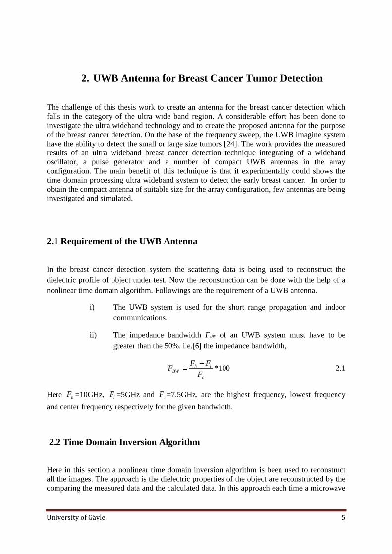
2. UWB Antenna for Breast Cancer Tumor Detection

The challenge of this thesis work to create an antenna for the breast cancer detection which

falls in the category of the ultra wide band region. A considerable effort has been done to

investigate the ultra wideband technology and to create the proposed antenna for the purpose

of the breast cancer detection. On the base of the frequency sweep, the UWB imagine system

have the ability to detect the small or large size tumors [24]. The work provides the measured

results of an ultra wideband breast cancer detection technique integrating of a wideband

oscillator, a pulse generator and a number of compact UWB antennas in the array

configuration. The main benefit of this technique is that it experimentally could shows the

time domain processing ultra wideband system to detect the early breast cancer. In order to

obtain the compact antenna of suitable size for the array configuration, few antennas are being

investigated and simulated.

2.1 Requirement of the UWB Antenna

In the breast cancer detection system the scattering data is being used to reconstruct the

dielectric profile of object under test. Now the reconstruction can be done with the help of a

nonlinear time domain algorithm. Followings are the requirement of a UWB antenna.

i) The UWB system is used for the short range propagation and indoor

communications.

ii) The impedance bandwidth FBW of an UWB system must have to be

greater than the 50%. i.e.[6] the impedance bandwidth,

100*c

lhBW

F

FFF 2.1

Here hF =10GHz, lF =5GHz and cF =7.5GHz, are the highest frequency, lowest frequency

and center frequency respectively for the given bandwidth.

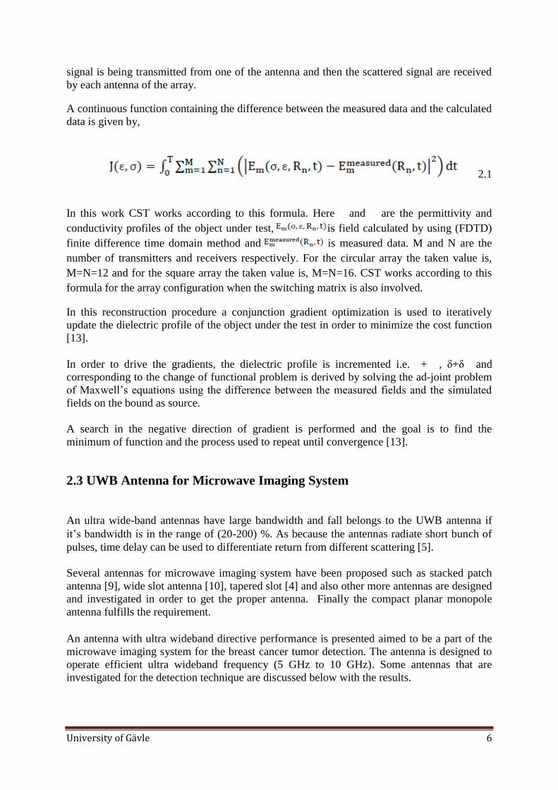
2.2 Time Domain Inversion Algorithm

Here in this section a nonlinear time domain inversion algorithm is been used to reconstruct

all the images. The approach is the dielectric properties of the object are reconstructed by the

comparing the measured data and the calculated data. In this approach each time a microwave


signal is being transmitted from one of the antenna and then the scattered signal are received

by each antenna of the array.

A continuous function containing the difference between the measured data and the calculated

data is given by,

2.1

In this work CST works according to this formula. Here and are the permittivity and

conductivity profiles of the object under test, is field calculated by using (FDTD)

finite difference time domain method and is measured data. M and N are the

number of transmitters and receivers respectively. For the circular array the taken value is,

M=N=12 and for the square array the taken value is, M=N=16. CST works according to this

formula for the array configuration when the switching matrix is also involved.

In this reconstruction procedure a conjunction gradient optimization is used to iteratively

update the dielectric profile of the object under the test in order to minimize the cost function

[13].

In order to drive the gradients, the dielectric profile is incremented i.e. + , δ+δ and

corresponding to the change of functional problem is derived by solving the ad-joint problem

of Maxwell‟s equations using the difference between the measured fields and the simulated

fields on the bound as source.

A search in the negative direction of gradient is performed and the goal is to find the

minimum of function and the process used to repeat until convergence [13].

2.3 UWB Antenna for Microwave Imaging System

An ultra wide-band antennas have large bandwidth and fall belongs to the UWB antenna if

it‟s bandwidth is in the range of (20-200) %. As because the antennas radiate short bunch of

pulses, time delay can be used to differentiate return from different scattering [5].

Several antennas for microwave imaging system have been proposed such as stacked patch

antenna [9], wide slot antenna [10], tapered slot [4] and also other more antennas are designed

and investigated in order to get the proper antenna. Finally the compact planar monopole

antenna fulfills the requirement.

An antenna with ultra wideband directive performance is presented aimed to be a part of the

microwave imaging system for the breast cancer tumor detection. The antenna is designed to

operate efficient ultra wideband frequency (5 GHz to 10 GHz). Some antennas that are

investigated for the detection technique are discussed below with the results.


2.3.1 Wide-slot Antenna

A wide slot antenna is being designed [10] and tested, which consists of an wide square slot in

the ground plain in one side of substrate with relative permittivity of 10.2 and on the other

side of the substrate is forked micro strip feed which splits below the slot, from 50 ohm feed

into two 100 ohm sections that excites the slot [15]. The total size of the antenna is

35mm*40mm and is simulated with the given frequency range 5GHz to 10GHz. Figure 3

shows the wide-slot antenna and figure 4 shows the reflection coefficient(S11) vs. entire

frequency graph for the wide-slot antenna.

Figure 3. The wide-slot antenna

Figure 4. Reflection coefficient vs. frequency for wide-slot antenna

Here in the graph we can see that the resonating frequency is at 8.25GHz then reflection

coefficient is increasing with the increasing of the frequency. After reaching the reflection

coefficient at 9.25GHz it‟s decreasing again with the increasing of frequency. The whole

bandwidth is performing well because the reflection coefficient is <-10dB for the entire


frequency range but the model is not suitable enough for the annular array configuration

because of large size.

2.3.2 Stacked Patch Antenna

A stacked patch antenna is being designed and investigated which consists of a micro-strip

line feeding slot, which in turns excites an arrangement of stacked patches. In the

configuration the slot feed is used to eliminate the inductance associate with a probe feed. The

patches sandwiching the lower permittivity substrate and their size is chosen because of lower

order resonance was achieved at either end of the desired frequency band [10]. Figure 5

shows the stacked patch antenna, and figure 6 shows the reflection coefficient (S11) vs. entire

frequency graph of the stacked patch antenna.

Figure 5. The stacked patch antenna

Figure 6. Reflection coefficient vs. frequency for stacked patch antenna


Here in the graph we can see that the resonating frequency is at 5.9GHz and than reflection

coefficient is increasing with the increasing of the frequency. At 7.7GHz the reflection

coefficient starts to decrease with the increasing of frequency and after reaching the reflection

coefficient at 8.2GHz it‟s increasing again with the increasing of frequency. By the

characteristics of the graph we can see that it‟s working as a dual band frequency because it‟s

have the two resonating point and 6.5 GHz to 7.9GHz, the whole bandwidth is showing the

reflection coefficient >-10dB. So that antenna is not performing well for the entire frequency

range.


3. Planar Monopole Antenna (PMA)

The investigation of the planar monopole antenna is influenced to focus on the planar shape in

the impedance bandwidth of the antenna. An optimization has to be done to get the best

parameter, so the designed applicator can handle the coupling medium and can also improve

the matching of the imaged object. Thus the increment of the dynamic range of the imaging

system can be done. The simulation performance of the single designed antenna have to be

compact in size so for array design it can shows the good impedance match and also low

mutual coupling for it‟s element. For the optimized antenna the performance we need to check

is, the electric energy density in different frequency over the entire frequency range, the E-

field distribution in different frequency over the entire frequency range, the Far-field

distribution and the SAR.

3.1 Reason of using PMA

After Investigating lot of antennas, Planar Monopole Antenna (PMA) is considered for breast

cancer detection system. The reasons are,

i) The wide bandwidth can be achieved with this type of antenna.

ii) The antenna have very simple structure.

iii) The size and shape of the antenna is very suitable for array design.

iv) Because of antenna‟s very small size it‟s easy to mount it in an ordinary plastic

casing.

v) It gives smooth electric field distribution through phantom

In the initial step a conventional reduced size PMA with an exponential taper for (5-10) GHz

band is designed. Some modification has been done in a design to get the better performance

such as a „ ‟slot has been introduced to the substrate and optimization is done to the all

parameters to get the best parameter.

Inductance is an undesirable quantity in this case. We have a pertial ground and a „ ‟ slot to

overcome this inductance. Lot of slot like as „Π‟, „┼‟, „▲‟ is being introduced to the system

and finally „ ‟ slot is taken because of performing well. It‟s working as a parallel plate

capacitor. Figure 7 shows the planar monopole antenna and figure 8 shows the graph

reflection coefficient (S11) vs. entire frequency) for finally designed model.


Figure 7. A Planar Monopole Antenna

Figure 8. Reflection coefficient versus frequency of Planar Monopole Antenna

Here in the graph we can see that the resonating frequency is at 5.7GHz and the whole

bandwidth is showing the reflection coefficient <-10dB. We observe one undesired reflection

peak at 9.75 GHz where the power transmission is 89% approximately. This is a negligible

mismatch and can be removed by further optimizing the feed point of coaxial cable.

3.2 Antenna Structure

Here we can see the following designed model of the antenna in CST. Figure 9(a) is showing

the top view of the antenna, figure 9(b) is showing the bottom view of the antenna and figure

9(c) is showing the side view of the antenna. On top view we have focused on the corrugated

radiator parameters, on the bottom view we have focused on the partial ground plain

parameters and on the side view we have focused on the substrate parameters. The parameters

of the introduced slot are discussed in both top view and bottom view.


Figure 9. (i) The top view of the antenna with corrugated radiator, (ii) The bottom view of the antenna with

partial ground, (iii) The side view of the antenna

3.3 Required Parameters

This antenna has two required parameters [13].

a. Lower band-edge frequency ( lf )

b. Bandwidth (frequency span in which 11S ≤-10dB)

3.3.1 Lower band-edge frequency ( lf )

The lower band-edge frequency of the PMA can be determined by equating the area of the planar

configuration [17]. The Lower band-edge frequency,

rBFf

L

l

2.7GHz 3.1

Here B is patch height, FL is micro strip feed-line height and the effective patch radius is r

(A/4), all the values of all parameters are considered in cm. That dielectric material increases

the effective dimension of the monopole leading to reduction in the lower band-edge

frequency.


3.3.2 Bandwidth (frequency span in which 11S ≤-10dB)

In this antenna design there are few parameters which influencing the bandwidth (frequency

span for which reflection coefficient is ≤-10dB) of PMA. First parameter is the effective patch

radius r. It has to be select properly otherwise the antenna will not exhibit wideband. [12],

[20]. Second parameter is the micro strip feed-line height FL and the third parameter is patch

height B.

3.4 Antenna’s Parameters Description

Here we have discussed all the parameters to the following table 1.

Description Parameters Dimensions(mm)

The patch height B 4.77

The patch width A 8.52

Patch thickness PX 0.2

Micro strip feed line height FL 5.25

Micro strip feed line width Fw 0.45

Substrate height SL 10.5

Substrate width Sw 9

Substrate thickness SX 0.64

Ground Height GL 4.77

Ground width GW 8.52

Ground thickness GX 0.2

Gap between the monopole and the ground P 0.48

Table 1. The list of parameters used in antenna designing


The calculation of the monopole is being performed following.

Calculations

The given frequency is, (5-10)GHz

The center frequency, cf = 7.5GHz

Speed of light, c= 300000000m/s

Length of the antenna is calculated as follows.

We know, λ=c / cf

=40mm

So for monopole, λ/4 = 10mm.

3.5 Optimization of designed parameters

In this design different parameter is been considerd and a finalized table is manipulated in

Table.2 such as, effect of the patch length ( B ), effect of ground plane length ( LG ), effect of

change of patch effective width ( A ), effect of gap between patch bottom edge and ground

plane ( P ), effect of change of feed-line width ( wF ) and effect of change of ground width ( wG

). Now those different parameters have been optimized and simulated in order to get the best

parameter for the designed antenna for the entire frequency. Different values of parameters

are chosen after simulating and optimizing in CST. Finally the best values are chosen. All

final values are chosen and given in table 1. There are different types of solovers in CST, but

Transient solver is used for antennas, transmission line and connectors. This is accurate and

fast process which leads to the CST MWS software [18]. The simulation results for the

different values of different parameters are explained below. Table.2 shows the obtained

results of the optimized antenna parameters.


Optimized parameters Best Chosen

Values(mm)

Resonating

frequency

(GHz)

Maximum

Reflection

coefficient(dB)

Effect of the patch length ( B ) 3.77 5.45 -11

Effect of Ground plane length ( LG ) 3.77 5.9 -11.2

Effect of patch effective width ( A ) 7.52 5.5 -11

Effect of gap between patch bottom edge

and ground plane ( P )

2.45 5.95 -11.8

Effect of feed-line width ( wF ) 0.55 5.75 -11

Effect of ground plain width ( wG ) 7.52 5.75 -10.9

Table 2. Results of the optimized antenna parameters

So now from the table 2 we can see all the results of the optimized parameters after simulation

and observation. The green curve performs the best results among all the parameters. We can

see from the table that the lowest reflection coefficient for the entire frequency rage is -11.8

dB and we got that for the changing of the gap between patch bottom edge and ground plane.

So when we keep all the parametes constant but the gap between patch bottom edge and

ground plane P =2.48 mm then we get the less reflection coefficient and the resonating

frequency is 5.95 GHz. So for P=2.48mm all the parameters can be taken to design the

antenna and to finalized it.

3.5.1 Effect of the patch length ( B )

For the optimization of the patch length, we know that by increasing the value of „ B ‟ we get

a lower value of the LF . When B = 4.77 mm, 4.27 mm or 3.77 mm we get the changes in the

length of feed-line. Figure 10 shows reflection coefficient (S11) vs. entire frequency graph for

different patch length ( B ).


Figure 10. frequency vs. reflection coefficient graph for different patch length ( B )

Now from the figure we can see that when B =3.77mm then the reflection coefficient is below

then -10dB over the entire frequency band of interest and the resonating frequency is

5.45GHz. So from the result it is clear that in this design both the achieved bandwidth and

lowest resonance frequency are dependent on the patch length ( B ).

Similarly we have explained different parameters one by one. The graphical representations

are given in the appendix.

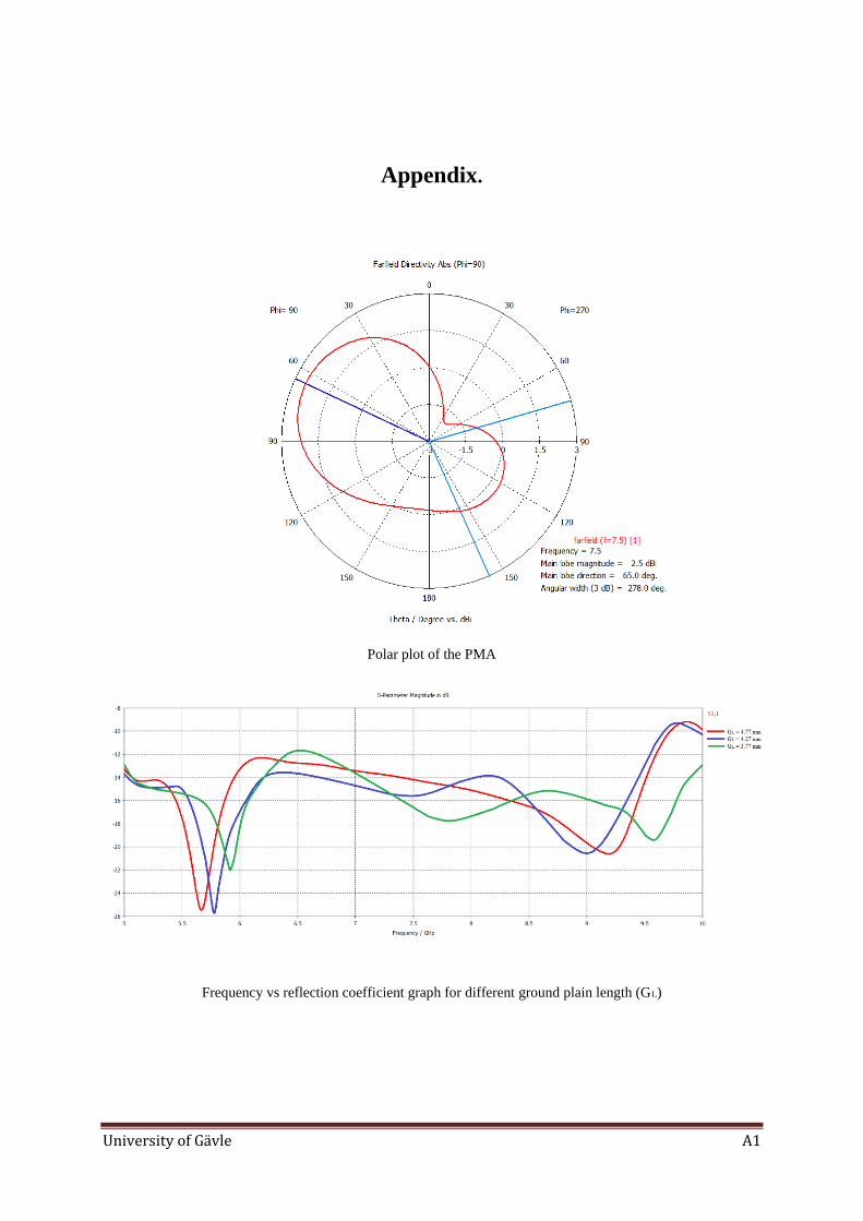
3.5.2 Effect of Ground plane length ( LG )

For different values of the ground plain length, LG = 4.77 mm, 4.27 mm or 3.77 mm we get

respective variation in the reflection coefficient. We conclude that as the value of LG

decreases, we get the antenna behaving more effectively with respect to reflection coefficient

(S11). Reflection coefficient (S11) vs. entire frequency graph for different ground plane

length LG is given in appendix. Also the best value for S11 is presented in Table 1

From the graph we can see that the changing ground plane length has also significant effect

on lowest resonance frequency. Increasing the ground plane length doesn‟t changes other

parameters. Now from the figure we can see that when LG =3.77mm then the reflection

coefficient < -10dB over the entire frequency band of interest and the resonating frequency is

5.9GHz.

3.5.3 Effect of patch effective width ( A )

For different values of the patch width, A = 8.52 mm, 8.02 mm or 7.52 mm we observe the

significant change in the reflection of antenna. We see that as the effective patch width is

decreased, we get an improved return loss over the desired frequency range. An elaborated

graph is given in appendix.


From the graph we can see that the changing effective patch width has significant effect on

resonance frequency and return loss. Increasing of the effective patch width doesn‟t changes

other parameters except reflection behavior of planar antenna. Now from the figure we can

see that when A =7.52mm then the reflection coefficient <-10dB over the entire frequency

band of interest and the resonating frequency is 5.5GHz. The finalized value for effective

width is given in table 1.

3.5.4 Effect of gap between patch bottom edge and ground plane ( P )

For different values of P = 0.48 mm, 1.48 mm or 2.48 mm making the changes in the

reflection of our proposed antenna. It is observed that as we increase the gap, a significant

change in the reflection coefficient is obtained. For example at the gap with 2.48mm we get

the maximum reflection value of -11.8dB which is the best value as shown in the table.1 a

graphical representation of this comparison is also explained in the appendix.

From the graph we can see that the changing of gap between patch bottom edge and ground

plane has significant effect on resonance frequency. It changes both the parameter of patch

length and feed-line height. Now from the figure we can see that when P =2.48mm and 1.48

then the reflection coefficient is below then -10dB over the entire frequency band of interest

and the resonating frequency is 5.95GHz and 5.85GHz.

3.5.5 Effect of feed-line width ( wF )

For different values of the feed width, wF = 0.35 mm, 0.45 mm or 0.55 mm we observe that

as we increase the feed-line width, we get good performance of antenna with respect to its

reflective behavior. As for example, we first chose the value to be 0.35mm the antenna was

reflecting the input power, as we then increased the feed width, we got further improvement

in the transmission of our proposed antenna and consequently a good reflection coefficient

was observed at 0.55mm feed width that we have shown in the table 1. Furthermore a

graphical presentation of this analysis is given in appendix.

From the graph we can see that the changing feed-line width has little effect on resonance

frequency. Increasing of the feed-line width doesn‟t changes other parameters except

reflection of antenna. Now from the figure we can see that when wF =0.55mm then the

reflection coefficient <-10dB over the entire frequency band of interest and the resonating

frequency is 5.72GHz.

3.5.6 Effect of ground plane width ( wG )

Further we have discussed the effect of the ground plane width on different parameters of

antenna. For different values of the ground plane width, wG = 8.52 mm, 8.02 mm or 7.52

mm. A graphical representation of frequency vs. reflection coefficient graph for different

ground plane width wG is given in the appendix. It is concluded that as the wG is reduced, a


corresponding change appears in the reflection of antenna. For example wG =7.52mm gives

us the best behavior of proposed antenna. At this specific value we get S11= -10.9dB. This is

a good selection for the performance of antenna.

From the graph we can see that the changing effective patch width also has little effect on

resonance frequency. Increasing of the effective ground width doesn‟t changes other

parameters except reflection coefficient. Now from the figure we can see that when wG

=7.52mm and 8.02mm then the reflection coefficient <-10dB over the entire frequency band

of interest and the resonating frequency is 5.76GHz and 5.7GHz.

3.6 Electric Energy Density

Eletric energy density is a term used for the amount of electric energy is being stored in given

PMA or region of space per unit volume. This is an action of stored energy at an unike

volume lavel. The charges repel each other during the charging process. The field picture of

the energy is that the energy is stored in the space between the conductors where there is an

electric field, E, present. Since the energy is thought of as being stored throughout a volume,

it makes sense to speak of the volume density of this energy, or the energy per unit volume.

Figure 11 shows the electrical energy density of a single antenna in the air.

Figure 11. The electrical energy density of a single antenna in air


From the figure we can see that the distribution of the electric energy through theh antenna is

very uniform for five different frequency over the entire frequency range. The unit of the

electric energy density is J/m^3 and by the color range we can see that in which part of the

antenna showing how much electric energy per unit volume. It‟s better if the highest range of

the antenna per m^3 area is below then 0.02J. Otherwist it‟s can burn the breast tissue.

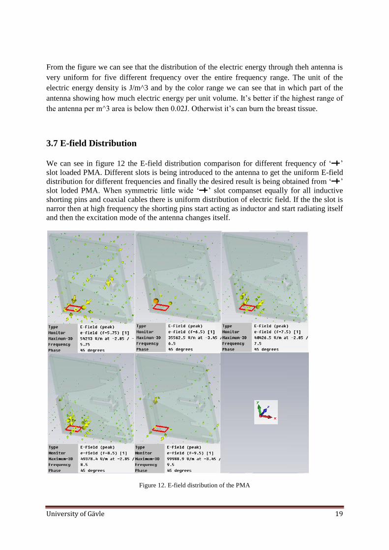
3.7 E-field Distribution

We can see in figure 12 the E-field distribution comparison for different frequency of „ ‟

slot loaded PMA. Different slots is being introduced to the antenna to get the uniform E-field

distribution for different frequencies and finally the desired result is being obtained from „ ‟

slot loded PMA. When symmetric little wide „ ‟ slot companset equally for all inductive

shorting pins and coaxial cables there is uniform distribution of electric field. If the the slot is

narror then at high frequency the shorting pins start acting as inductor and start radiating itself

and then the excitation mode of the antenna changes itself.

Figure 12. E-field distribution of the PMA


We can see from the figure that the maximum focusing point of the arrow is the feeding point

and then it‟s scattered uniformly to the whole part of antenna. Furthermore the cut between

the bottom edge of the patch and the upper edge of the ground plain plays a vital role to

overcome undesired inductance in conjunction with the little wide „ ‟ slot. The basic goal in

our design is to achieve the uniform electric field distribution thorough out the phantom. So

that the tumour residing in any part of the phantom could be identified by the superposition of

the uniform electric field.

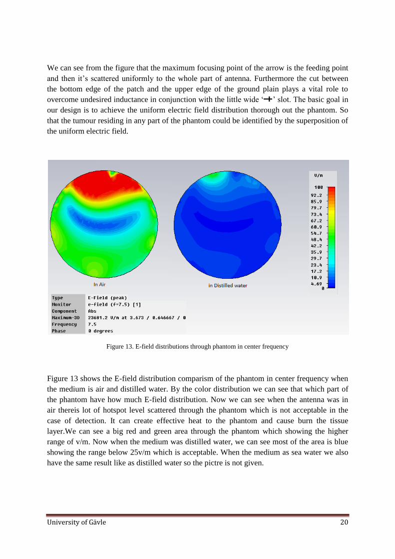
Figure 13. E-field distributions through phantom in center frequency

Figure 13 shows the E-field distribution comparism of the phantom in center frequency when

the medium is air and distilled water. By the color distribution we can see that which part of

the phantom have how much E-field distribution. Now we can see when the antenna was in

air thereis lot of hotspot level scattered through the phantom which is not acceptable in the

case of detection. It can create effective heat to the phantom and cause burn the tissue

layer.We can see a big red and green area through the phantom which showing the higher

range of v/m. Now when the medium was distilled water, we can see most of the area is blue

showing the range below 25v/m which is acceptable. When the medium as sea water we also

have the same result like as distilled water so the pictre is not given.


3.8 Far-field Distribution

By the far-field distribution we can see the radiation pattern of the PMA. The radiation

intensity is not same for the antenna according to all direction and position. So the term near-

field or far-field can be used to describe the radiation density of the antenna to the desired

distance. There are different types of radiation pattern of the antenna like as, directional,

beam. Etc. If the antenna is radiating in all direction then the used term is omni-directional. It

can show the radiation pattern of the antenna towards a specific direction [22]. Now another

two terms can be introduced in radiation pattern as main lobes and minor lobes. A Main lobe

defines the maximum radiation existing area and a minor lobe defines the minimum radiation

existing area [23]. In Figure 14 we can see the radiation patter of PMA at 7.5 GHz. We can

see the absolute value of the directivity of the antenna both in 3D and 2D plot. The polar plot

is explained in appendix. In Figure 15 we can see for theta/phi direction and in figure 16 we

can see for phi/theta direction.

3.8.1 Directivity of the antenna (3D and 2D)

Figure 14. The radiation pattern of PMA at 7.5 GHz


3.8.2 Directivity of the antenna in Theta/Phi direction (3D and 2D)

Figure 15. The radiation pattern of PMA on theta/phi direction at 7.5 GHz

3.8.3 Directivity of the antenna in Phi/Theta direction (3D and 2D)

Figure 16. The radiation pattern of PMA on phi/theta direction at 7.5 GHz


3.9 Specific Absorption Rate (SAR)

The SAR is an amount of the power absorbed by the medium per unit of the mass [21]. In

breast cancer detection SAR is the standard that can put some limit to the maximum amount

of power absorbed by the breast tissue. SAR can be calculated by the following equation.

2

ESAR , 3.1

Where is the conductivity of the material in S/m, E is the electric field intensity in V/m and

is the mass density in Kg/ 3m . From the equation it‟s clear that the focusing point is the

amplitude of the electric field intensity and not the phase. Distilled water and sea water is

considered as the best medium in water bolus. Figure 17 shows the normalized SAR

distribution with a single antenna through phantom when the medium is distilled water. An

explanation of the picture for the normalized SAR distribution with a single antenna through

phantom when the medium is sea water is given in appendix. The frequency separation is

being done to see the SAR distribution in different frequency

Figure 17. Normalized SAR distributions with a single antenna in distilled water through phantom


4. Antenna Array Design

For microwave breast cancer detection system the phantom is illuminated with the continuous

electromagnetic radiation of the single applicator from the different direction. For the annular

array designing the antenna is placed to the array with proper direction and distance and

immersed in to a water bolus. All the antennas are connected with the wave guide port. When

antennas get close to each other the mutual coupling occur between antennas both in receiving

and transmitting mode. The requirement of the coupling is at least -20dB between all the

neighbor radiators in the array [14].

The antenna array can be configured by 8*1, 12*1 or 16*1 setup. For the minimum number of

applicators can be obtained in 8*1 configuration which can focus better energy for lower

range of frequencies (434MHz-800MHz) only. For more lower or upper frequency limit there

could be an irregular power flow with this configuration and results no uniform E-field

distribution and also no uniform SAR distribution and high level of hotspots could be

achieved at the surface of phantom. Now to work with high frequency range and to get

uniform SAR distribution the modification can be done and the configuration can be

improved by 12*1 or 16*1 configurations.

4.1 The Water Bolus Model

The circular array radiators are used for the breast cancer detection also required water bolus.

The water bolus is the perfect medium to cool down the outer surface of the tissue of the

phantom and also it‟s used to cool down the radiating antenna. A number of radiators in the

circular array excite simultaneously to all individual frequencies, causing a strong heating

effect at a single target point deep inside to the phantom. Due to the irritating effect of the

radiator the surface of the breast tissue can burn or have some undesired effect. This effect

could be reduced by using the water bolus filled with cooled circulating water. All the

radiators are used to immerse in different matching liquids of different permittivity. The

radiated power is being absorbed by the phantom after passing through the matching liquid.

The size and shape of the water bolus, the height and diameter of different matching liquids

depends on the given frequency which is used according to the surface of the breast tissue. In

our CST setup we have used the thickness of the water bolus as 20mm and the height as

60mm. The inner diameter of the water bolus is 100mm same as the diameter of the phantom

and outer diameter is 140mm. Figure 18 shows the water bolus model used in our CST.


Figure 18. The water bolus model

4.2 Proposed Circular Antenna Array:

While designing the circular antenna array, we had to keep two parameters on Mind,

i) The size of the circumferential array configuration

ii) The distance between two adjacent antenna

Figure 19 shows the block diagram of a designed antenna array (top view).


Figure 19. Top view of antenna array

Now we have the thickness of the water bolus is 20mm. So the total radius of the array= the

radius of the phantom + the thickness of the water bolus = 50mm+20mm = 70mm.

So the size of the circumferential array is,

rC 2

=2* *70

=439.6mm

Now the distance between two adjacent antennas is,

( r2 /12)- (the width of one antenna) = (439.6/12)-9

=27.63mm

In CST one antenna is being designed and 11 copies of one antenna is being made, given to an

antenna array and simulated in air, different matching liquids and with different dielectric


properties. A circular chamber is used to hold the total array configuration and the water bolus

is used to hold the matching liquids and mount antennas. The chamber is made of a plastic

material having the permittivity of 1.2 and conductivity of 1Exp-16 S/m. All the antennas are

connected through wave guide ports of 50 ohm impedance. With all the radiators a discreet

port is attached to the feeding point which is acting as waveguide port. The complete antenna

array setup in CST is shown in Figure 20.

Figure 20. The complete antenna array setup in CST

Now the diameter of the phantom is 100mm. So the radius of the phantom is 50mm.

So the size of the circumferential phantom is,

rC 2

=2* *50

=314mm


4.3 Reflection Coefficient of antennas among the array

This is the primary requirement of the entire antenna in the array that the reflection coefficient

is below -10 dB over the entire frequency band. Now in the breast cancer detection system all

the antennas in the designed array are close proximity to each other and this cause mutual

coupling among all radiators. Increasing of the mutual coupling in the array also cause to

increase their reflection coefficient. To achieve the desired reflection coefficient the distance

between the neighbor antennas is optimized and adjusted perfectly. The medium of the water

bolus is also creating effect to reflection coefficient. So higher permittivity material is

preferable to have better result. We can see in Figure 21 the Reflection coefficients (S11) vs.

entire frequency graph of 4 neighbor antennas in sea water among the array and in Figure 22

we can see the (Reflection coefficients vs. frequency) graph of 4 neighbor antennas in

distilled water among the array.

Figure 21. Reflection coefficients vs frequency of 4 neighbor antennas in sea water among the array

Figure 22. Reflection coefficients vs. frequency of 4 neighbor antennas in distilled water among the array


From the above figure 21 and figure 22, we can see that the array of antenna is perfectly

transmitting the power inside the muscular phantom because the mutual coupling between

two adjacent antennas is below -20dB, so the power level is more than 90% which guaranties

the overall good performance of antenna [14].

4.4 Performance of the antenna array

The antenna array has to be designed perfectly and have to sit in the water bolus so we have

less mutual coupling and uniform E-filed distribution.

4.4.1 Mutual coupling among the antenna array

We can define the term mutual coupling as, when two or more neighbor antennas come close

to each other and when one antenna is transmitting a part of energy, another is receiving and it

exists both in transmitting and in receiving mode. Now among the annular array configuration

in transmitting mode one antenna used to radiate a part of energy which is received by the

other is known as mutual coupling. Mutual coupling decreases when the distance between

neighbor antennas increases. Mutual coupling depends on the following factors [19].

i). Radiation pattern of the antenna

ii). separation between antennas (both horizontally or vertically)

iii). Antennas orientation on the array.

4.4.1.1 Mutual coupling in air

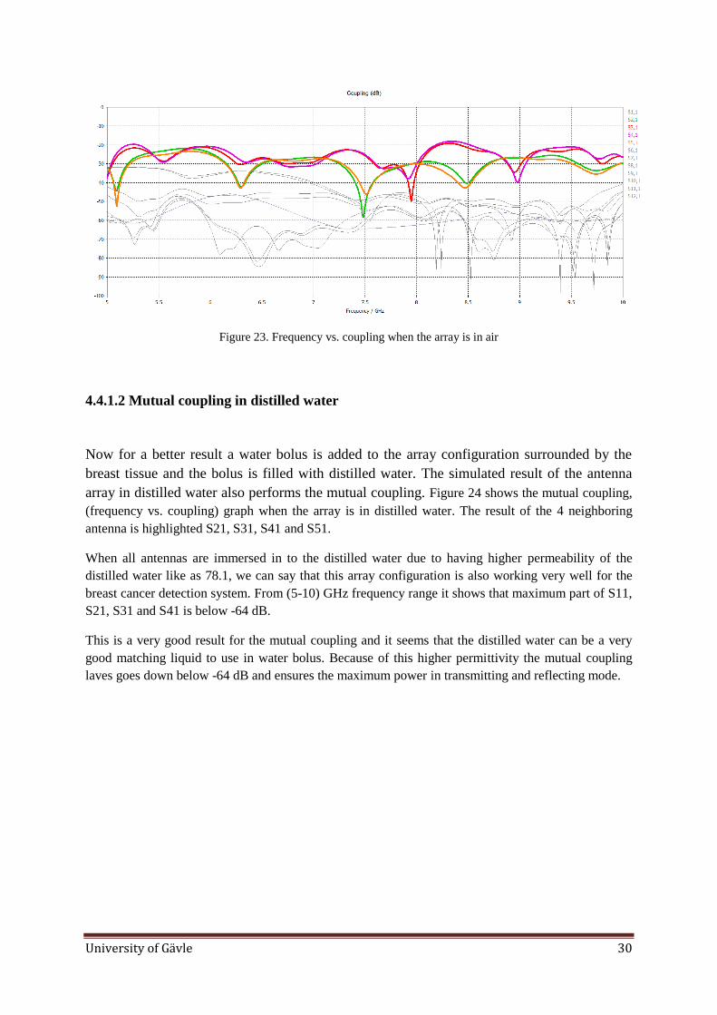
The simulated result of the antenna array in air performs the mutual coupling. Figure 23 shows

the mutual coupling, (frequency vs. coupling) graph when the array is in air. The result of the

neighboring antenna is highlighted S21, S31, S41 and S51.

This is evident to say that this array configuration is not bad to use for the breast cancer detection

system. From (5-10) GHz frequency range it shows that maximum part of S21, S31, S41 and S51 is

below -20 dB.


Figure 23. Frequency vs. coupling when the array is in air

4.4.1.2 Mutual coupling in distilled water

Now for a better result a water bolus is added to the array configuration surrounded by the

breast tissue and the bolus is filled with distilled water. The simulated result of the antenna

array in distilled water also performs the mutual coupling. Figure 24 shows the mutual coupling,

(frequency vs. coupling) graph when the array is in distilled water. The result of the 4 neighboring

antenna is highlighted S21, S31, S41 and S51.

When all antennas are immersed in to the distilled water due to having higher permeability of the

distilled water like as 78.1, we can say that this array configuration is also working very well for the

breast cancer detection system. From (5-10) GHz frequency range it shows that maximum part of S11,

S21, S31 and S41 is below -64 dB.

This is a very good result for the mutual coupling and it seems that the distilled water can be a very

good matching liquid to use in water bolus. Because of this higher permittivity the mutual coupling

laves goes down below -64 dB and ensures the maximum power in transmitting and reflecting mode.


Figure 24. Frequency vs. coupling when the array is immersed in distilled water

4.4.1.3 Mutual coupling in sea water

Now again for a better result the same formula is applied. The water bolus is added to the

array configuration surrounded by the breast tissue and the bolus is filled with sea water this

time. The simulated result of the antenna array in sea water also performs much better result

for the mutual coupling. Figure 25 shows the mutual coupling, (frequency vs. coupling) when the

array is immersed in sea water. The result of the neighboring antenna is highlighted S21, S31, S41 and

S51.

When all antennas are immersed in to the sea water due to having higher permeability this is evident to

say that this array configuration is also working much better for the breast cancer detection system.

From (5-10) GHz frequency range it shows that maximum part of S21, S31, S41 and S51 is below -

62dB.

Figure 25. Frequency vs. coupling when the array is immersed in sea water


This is also very good result for the mutual coupling like as the medium of distilled water and it seem

that the sea water can also be a very good matching liquid to use in water bolus. Having the higher

permittivity of sea water as 74, it performs well for mutual coupling and the mutual coupling laves

goes down below -62 dB and ensures the maximum power in transmitting and reflecting mode.

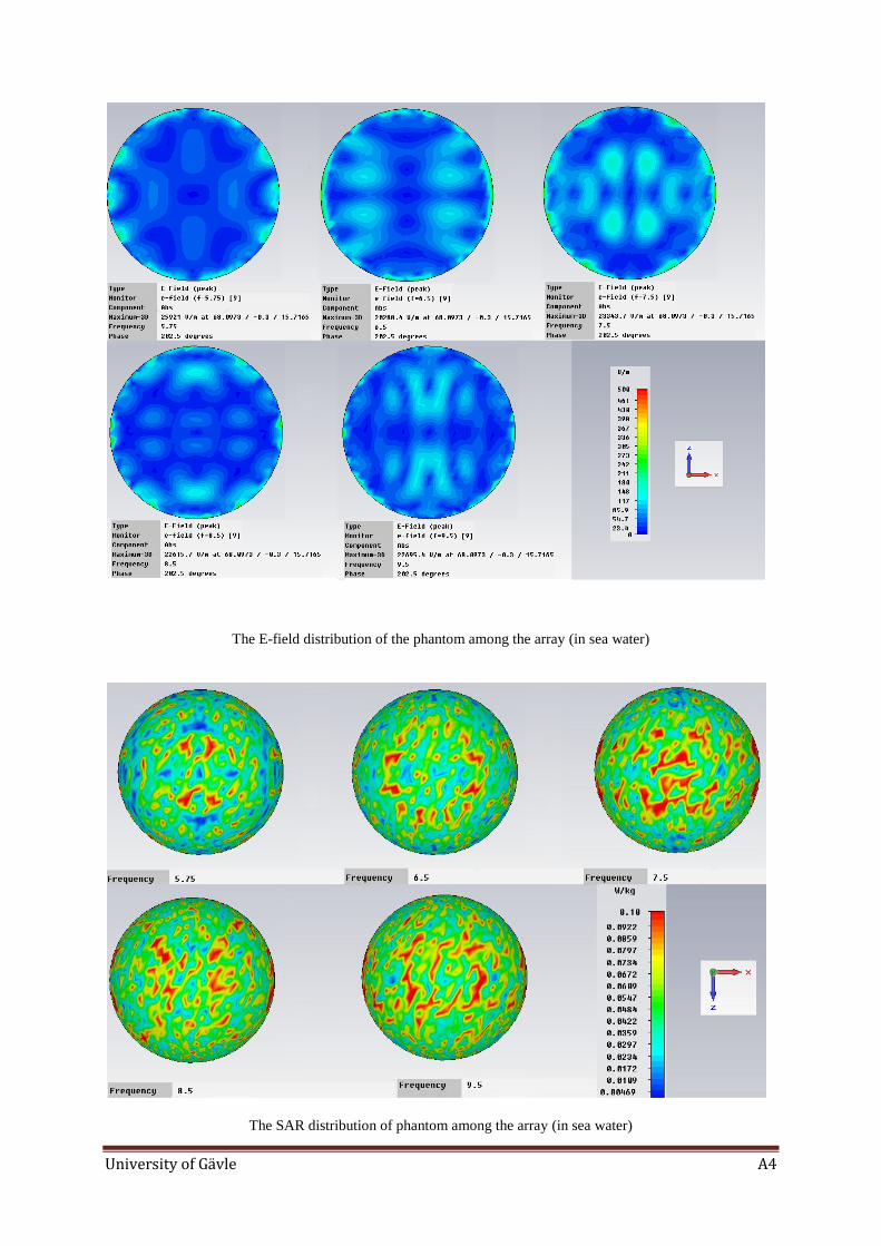
4.4.2 E-field distribution among the antenna array

For the breast cancer detection technique it‟s required that the E-field distribution is produced

deep inside the breast tissue. To the following application number of transmitter is illuminate

object under test. The requirement of a single applicator is to distribute the E-field both

horizontally and vertically by covering most of the area of the object under test. We have used

12 antennas in our designed array and simulated. We can see in Figure 26 the E-field

distribution when the medium is distilled water. From the figure it can be clearly observed

that the electric field distribution inside the muscular phantom is uniformly distributed. This

phenomenon permits us to say that the accurate detection can be done of deeply seated small,

medium or large size tumors. A picture of the E-field distribution when the medium is

distilled water is explained in appendix.

Figure 26. The E-field distribution of the phantom among the array in distilled water


4.5 SAR distribution of the phantom among the antenna array

Figure 27 shows the SAR distribution of phantom among the array when the medium is

distilled water in the water bolus and the SAR distribution of phantom among the array when

the medium is sea water in the water bolus is explained in appendix. The highest range is

given as 0.1 W/Kg at the surface of the phantom which is acceptable for the case of detection.

The higher range of the SAR distribution can burn the breast tissue and can destroy it. The

focusing area is changing with respect to the changing of lower frequency to higher

frequency. Higher frequencies are used to detect for the deeply seated small size tumor due to

small wavelength and lower frequencies are used to detect for the deeply seated medium and

large size tumors due to large wavelength. In our case the designed single applicator works

for the frequency range (5-10) GHz since it gives uniform SAR distribution deep inside the

phantom.

Figure 27. The SAR distribution of phantom among the array in distilled water

Now for example if we take the values as,

E-field intensity, E= 20 V/m

Conductivity of breast, = 0.2 S/m


Mass density of breast, = 998 Kg/ 3m

Then we have the value of,

2E

SAR

= 998

20*2.02

=0.08W/Kg

4.6 Proposed antenna array design parameters in different medium

(i) Table 3 shows the electrical properties of the medium used in the array

Used Medium Permittivity (εr) Conductivity (ζ)S/m Mass density( )kg/m^3

ML1(Distilled

Water)

78.1 5.55e-006 998

ML2(Sea Water) 74 3.53 1000

Air 1 08e-15 1.204

Plastic Chamber 1.2 10e-16 --------

Table 3 Electrical properties of the medium

(ii)Table 4 shows the description of the antenna array design parameters.

Parameters Description Values in mm

Rphn Radius of the phantom 50

Hphn Height of the phantom 50

Cph Circumference of the phantom 314

Din Inner circle diameter of the water bolus 100

Dut Outer circle diameter of the water bolus 140

Tpc Thickness of the plastic chamber 2


Car Circumference of the antenna array 439.6

D The distance between neighbor antennas 27.63

Table 4 The antenna array design parameters


5. Conclusion

We have developed a simplified PMA model to simulate for a breast cancer detection using

an UWB microwave imagine method. Then the following model has been given to the

proposed array configuration and simulated. During this selection process lot of antennas is

being verified to prefer the most suitable one. The results that are presented here for the UWB

antenna array is very feasible and can get high contrast and high resolution. It‟s observed

water is the universal solution in water bolus and both sea water and distilled water gives the

better performance. Both Circular array and square array can be used in this setup but because

of more feasibility circular array configuration is chosen. As the diameter of the phantom is

only 100mm, so in array configuration the work is being continued keeping 12 applicators.

Another reason to have less number of antennas is to avoid mutual coupling. Nowadays the

planer antenna is widely used in most of the biomedical field because of their characteristics.

They are low profile, light weight and easy to manufacture. For the high frequency purpose

it‟s a best choice.


6. Future Work

The future work of this thesis work will involve the matter of manufacturing the designed

antenna. Regarding the matter we have already contacted some companies in China and

Germany but it cost like several hundred USD. So we contacted KTH and got to know that

Rogers substrate is not available in Swedish companies but in Belgium. But we are trying to

get the responsible person and to manufacture it so we can make a comparison between the

simulated result and the manufactured measurement result. And in future for clinical

experimental system it will be developed and will be tested at hospital.


References

[1] A. Fhager, “Microwave tomography”, Ph.D. dissertation, Department of signals and

systems, University of Chalmers and Technology, Gothenburg, Sweden, 2006.

[2] S. C. Hagness, E. J. Bond, X. Li and B. D. Van Veen,“ Microwave imaging via space-time

beam forming for early detection of breast cancer,” IEEE Trans. Antenna propag., vol. 51,

no.8, pp. 1690-1705, August 2003.

[3] Q. H. Liu, et al., “Active microwave imaging. I. 2-D forward andinverse scattering

methods,” IEEE Trans. Microwave Theory and Techniques, vol. 50, no.1, pp. 123-133, Jan.

2002.

[4] Y. Wang, A. A. Bakar, M. E. Bialkowski, “Compact Tapered Slot Antennas for UWB

Microwave Imaging Applications‟‟IEEE Microwave Radar and Wireless Communications

(MIKON), pp. 1-4, August 2010.

[5] D. Ghosh, M. C. Taylor, T. K. Sarkar, M. C. Wicks and E. L. Mokole, “Transmission and

reception by ultra wideband antennas,” IEEE antennas and propagation magazine, vol. 48,

no. 5, pp. 67-99, October 2006.

[6] Fractional Bandwidth (FBW), Available at,

http://www.antenna-theory.com/definitions/fractionalBW.php.

[7] National Breast Cancer Coalition (NBBC) published in 2004, Available at,

http://www.stoobreastcancer.org.

[8] X. Zeng, “Ultra wideband time domain system for microwave tomography”, Licentiate

thesis, Depertment of Signals and Systems, University of Chalmers and Technology,

Gothenburg, Sweden, 2010.

[9] R. Nilavalan, I. J. Craddock, A. Preece, J. Leendertz and R. Benjamin “Wideband

Microstrip Patch Antenna Design for Breast Cancer TumourDetection” Department of

Medical Physics,University of Bristol, UK, April 2007.

[10] I. J. Craddock, J. A. Leendertz, A Preece, D. Gibbins, M. Klemm, and R. Benjamin, “A

comparison of a wide-slot and a stacked patch antenna for the purpose of breast cancer

detection,” IEEE Trans. on Antennas and Propagation, vol. 58, no. 3, pp. 665-674, 2010.

[11] M. Persson, H. Zirath, X. Zeng, A. Fhager, P. Linner ,” Accuracy Investigation of an

Ultra-Wideband Time Domain Microwave Imaging System”, Department of Signals and

Systems, Chalmers University of Technology, Gothenburg, Sweden, 2011.

http://ieeexplore.ieee.org/xpl/mostRecentIssue.jsp?punumber=5523194

http://ieeexplore.ieee.org/xpl/mostRecentIssue.jsp?punumber=5523194

http://www.antenna-theory.com/definitions/fractionalBW.php


[12] C. J. Fox, P. M. Meaney, F. Shubitidze, L. Potwin, and K. D. Paulsen,“Characterization

of an implicitly resistively-loaded monopole antennain lossy liquid media,” International

Journal of Antennas and Propagation, Article ID 580782, 2008.

[13] P. Hashemzadeh, A. Fhager and M. Persson, “Experimental investigation of an

optimization approach to microwave tomography”, Electromagnetic Biology and Medicine,

vol. 25, issue 1, pp. 1-12, 2006.

[14] J. Yu, M. Yuan and Q.H. Liu, “A wideband half oval patch antenna for breast imaging”,

Progress in electromagnetics research, vol. 98, pp. 1-13, January 2009.

[15] J.-Y. Sze and K.-L.Wong, “Bandwidth enhancement of a microstripline-fed printed

wide-slot antenna,” IEEE Trans. Antennas and Propagation, vol. 49, pp. 1020-1024, July

2001.

[16] A. Abbosh, "Directive antenna for ultra wideband medical imaging systems," J.

Antennas and Propagation, vol. 2008, Article ID 854012, 2008.

[17] N. P. Agrawall, G. Kumar, and K. P. Ray, “Wide-band planar monopole antennas,” IEEE

Transa. on Antennas and Propagation, vol. 46, no. 2, pp. 294–295, 1998.

[18] Computer Simulation Technology, Available at,

http://www.cst.com/Content/Products/CST_S2/Overview.aspx.

[19] C. A. Blanis, “Antenna theory analysis and design”, New York: John Wiley & Sons, Vol.

24, pp. 28-29, January, 2003.

[20] A. Fhager, P. Hashemzadeh, and M. Persson, “Reconstruction quality and spectral

content of an electromagnetic time-domain inversion algorithm,” IEEE Trans.

Biomed.Engineering, vol. 53, no. 8 pp. 1594–1604, August 2006.

[21] M. A. Stuchly, M. Okoniewski, „„A study of the handset antenna and human body

interaction.‟‟ IEEE Trans. microwave Theory Techl, MTT-44, no.

10, pp.1855-l864, 1996.

[22] J. D. Kraus,“Antennas”,SecondEdition,Tata McGraw-Hill Publications. ISBN 0-07-

035422-7, 2001.

[23] K.D. Prasad and Prasad, “Introduction to Antenna and Wave Propagation”, Second

Edition, Satya Publication, 2008.

[24] W. Liu, H. M. Jafari, S. Hranilovic and M. J. Deen,“Time Domain Analysis of UWB

Breast cancer Detection‟‟ Department of Electrical and Computer Engineering, McMaster

University, Hamilton, Canada. L8S4K1, 2006.

http://www.cst.com/Content/Products/CST_S2/Overview.aspx

University of Gävle A1

Appendix.

Polar plot of the PMA

Frequency vs reflection coefficient graph for different ground plain length (GL)


Frequency vs reflection coefficient graph for different patch width (A)

Frequency vs reflection coefficient graph for different values of gap between patch bottom edge and ground

plain (P)

Frequency vs reflection coefficient graph for different feed-line width (FW)


Frequency vs reflection coefficient graph for different ground plain width (Gw)

Normalized SAR distribution with single antenna in distilled water through phantom


The E-field distribution of the phantom among the array (in sea water)

The SAR distribution of phantom among the array (in sea water)

an uwb antenna array for breast cancer detection457396/fulltext01.pdf · an uwb antenna array for...

Documents