1

Modeling of two-dimensional DNA display

Ana-Maria FLORESCU (1), Marc JOYEUX (1) and Bénédicte LAFAY (2)

(1) Laboratoire de Spectrométrie Physique (CNRS UMR5588), Université Joseph Fourier

Grenoble 1, BP 87, 38402 St Martin d’Hères, France

(2) Laboratoire Ampère (CNRS UMR5005), Université de Lyon, Ecole Centrale de Lyon, 36

avenue Guy de Collongue, 69134 Ecully, France

Corresponding author :

Marc JOYEUX

Laboratoire de Spectrométrie Physique (CNRS UMR5588)

Université Joseph Fourier Grenoble 1

BP 87

38402 St Martin d’Hères

France

Email : Marc.Joyeux@ujf-grenoble.fr

Phone : (+33) 476 51 47 51

Fax : (+33) 476 63 54 95

2

Abstract : 2D display is a fast and economical way of visualizing polymorphism and

comparing genomes, which is based on the separation of DNA fragments in two steps,

according first to their size and then to their sequence composition. In this paper, we present

an exhaustive study of the numerical issues associated with a model aimed at predicting the

final absolute locations of DNA fragments in 2D display experiments. We show that simple

expressions for the mobility of DNA fragments in both dimensions allow one to reproduce

experimental final absolute locations to better than experimental uncertainties. On the other

hand, our simulations also point out that the results of 2D display experiments are not

sufficient to determine the best set of parameters for the modeling of fragments separation in

the second dimension and that additional detailed measurements of the mobility of a few

sequences are necessary to achieve this goal. We hope that this work will help in establishing

simulations as a powerful tool to optimize experimental conditions without having to perform

a large number of preliminary experiments and to estimate whether 2D DNA display is suited

to identify a mutation or a genetic difference that is expected to exist between the genomes of

closely related organisms.

3

1 - Introduction

Two-dimensional (2D) DNA display was first described by Fisher and Lerman [1-3].

This is an electrophoresis technique, which consists in separating DNA fragments in two

steps, according first to their size and then to their sequence composition. The first step uses

traditional slab electrophoresis, for example in agarose or polyacrylamide gels. Collisions

between DNA and the gel reduce the mobility of DNA fragments, so that the gel acts as a

sieve and the electrophoretic mobility becomes size-dependent, with smaller molecules

generally going faster than large ones [4]. In the second dimension, fragments of identical

length are separated on the basis of their sequence composition, thanks to a gradient of either

temperature (TGGE : temperature gradient gel electrophoresis) or the concentration of a

chemical denaturant, e.g., a mixture of urea and formamide (DGGE : denaturing gradient gel

electrophoresis), both methods being closely related (see [5,6] and below). The effective

volume of denaturated regions being larger than that of double-stranded ones, the mobility of

a given fragment decreases as the number of open base pairs increases. Since AT-rich regions

melt at lower temperatures than GC-rich ones, GC-rich fragments usually move farther than

AT-rich ones.

Although 2D DNA display has recently been applied to the comparison of the

genomes of closely related bacteria [7-9], this method is still essentially empirical and

simulations have only been used to a very limited extent to plan experiments and interpret

results [10-12]. In particular, it has been shown only recently [12] that the final relative

positions of DNA fragments in 2D display experiments can be predicted with satisfying

precision using a model that combines step-by-step integration of the equation of motion of

each fragment and the use of the open source program Meltsim [13] to estimate the number of

open base pairs at each step of the DGGE phase. This kind of simulations will therefore

4

certainly develop further, in order to help optimize experimental conditions (denaturing

gradient range, electrophoresis duration, etc) without having to perform a large number of

tedious preliminary experiments, and to predict whether 2D DNA display is a convenient tool

to identify a given mutation or a genetic difference that is expected to exist between the

genomes of closely related organisms.

The goal of this paper is to extend the results presented in [12] along several lines.

First, these results were obtained by modifying one parameter in existing formulae for the

mobility of the DNA fragments during each phase of the 2D display process [5,14,15]. The

point is that the formula, which was used to estimate the mobility of the fragments during

electrophoresis along the first dimension, is rather complex and involves many parameters

[14,15]. It is therefore not ideally suited for fitting purposes. We will show that the

corresponding procedure can be greatly simplified without deteriorating the quality of

predictions. Moreover, calculations in [12] disregarded absolute positions and considered only

relative ones. This may be dangerous, because the positions of all fragments will be badly

predicted if, by lack of chance, the displacement of one of the two fragments that serve as a

basis to define relative positions is badly modeled. In addition, while it is indisputable that

traditional electrophoresis along the first dimension is a process that is linear with respect to

both time and distance, which allows one to use relative instead of absolute positions, this is

no longer the case for the second dimension : denaturation is indeed a very abrupt process, so

that use of relative coordinates becomes rather questionable. We will show in this paper that it

is possible to handle absolute rather than relative positions, provided that one modifies the

relation, which is used to estimate the equivalent temperature at a given position of the

denaturing gradient gel, i.e., for a given concentration of the chemical denaturant [6,16,17].

Last but not least, we adjusted all the parameters of the model, in order to get a global view of

its capabilities and limitations. It will in particular be shown that, while the model is capable

5

of predicting the final positions in the second dimension with an average error smaller than

experimental uncertainties, the number of base pairs that are open at the end of the

electrophoresis experiment can nevertheless not be estimated accurately.

The remainder of this article is organized as follows. The simulation procedure is

sketched in Sect. 2. Simulation of the separation according to size (first dimension) and

sequence composition (second dimension) is next discussed in Sect. 3. We finally conclude in

Sect. 4.

2 – Materials and methods

According to the definition of mobility, the position y of sequence s at time t in a

constant electric field E satisfies

( )Eysdt

dy,µ= . (2.1)

If the mobility ( )ys,µ depends uniquely on the sequence s and not on position y, as is the

case for the standard electrophoretic set-up in the first dimension, integration of Eq. (2.1) is

straightforward and leads to

( ) ( ) ( ) tEsyty µ=− 0 . (2.2)

In contrast, if the mobility ( )ys,µ depends on both the sequence s and position y, as is the

case for TGGE and DGGE, then Eq. (2.1) must be integrated step by step according to

( ) ( ) ( )( ) dtEtystydtty ,µ+=+ . (2.3)

In this work, we integrated such equations of motion for the 40 fragments already discussed in

[12], which were obtained from the site-specific restrictions of λ-phage genomic DNA using

EcoRI, Eco47I, Eco91I, HindIII and PstI, respectively. As reported in the first columns of

Table 1, the size of these fragments varies between 1929 and 23130 base pairs, and their GC

6

content between 36.0% and 58.9%. For the first separation (according to size), we plugged the

experimental values of the electric field (E=2 V/cm) and the total electrophoresis time (t=8 h)

in Eq. (2.2). For the second separation (according to sequence composition), we integrated

Eq. (2.3) with the experimental value E=7 V/cm for 44 h by steps of 7 mn and checked that

results do not vary when the total integration time is increased to 80 h and the time step

lowered to 1 mn. We also checked that these results are similar to those obtained with an

integration time of 24 h, which coincides with the experimental duration, and concluded that

DNA sequences were already stopped at the end of the electrophoresis experiments.

As will be seen in more detail in Sect. 3.2, the calculation of ( )( )tys,µ during DGGE

requires the estimation of the number of open base pairs of sequence s at a temperature T

which has the same denaturation effect as the local concentration of denaturant. This was

achieved as in [12] by using the open source program MeltSim [13], which is based on

Poland’s algorithm [18] and Fixman and Freire’s speed up approximation [19]. We used the

set of thermodynamic parameters of Blake and Delcourt [20] and set the positional map

resolution to 1, which corresponds to the highest possible calculation precision for the number

of open base pairs. The influence of the remaining free parameter of the program, namely the

salt concentration [Na+], will be discussed in detail in Sect. 3.2.

At last, the mobility ( )ys,µ is expressed for both electrophoresis steps as a function of

a certain numbers of parameters, which need to be adjusted to reproduce experimental results

accurately. Eq. (2.2) and the step by step integration of Eq. (2.3) were therefore embedded in

a refinement loop based on the gradient method, in order to vary these parameters so as to

minimize the root mean square deviation between experimental positions and those calculated

from Eqs. (2.2) and (2.3).

3 – Results and discussion

7

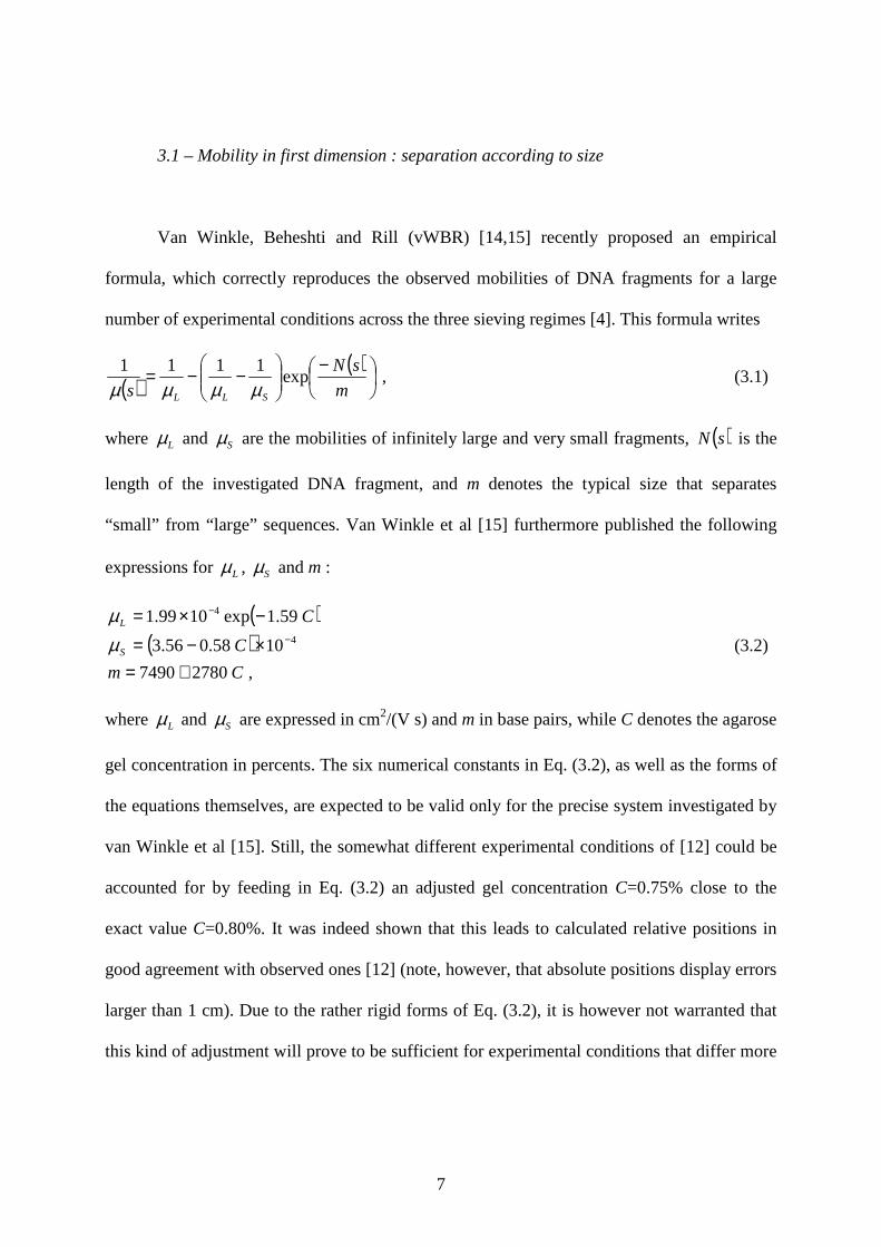
3.1 – Mobility in first dimension : separation according to size

Van Winkle, Beheshti and Rill (vWBR) [14,15] recently proposed an empirical

formula, which correctly reproduces the observed mobilities of DNA fragments for a large

number of experimental conditions across the three sieving regimes [4]. This formula writes

( )( )

−

−−=

m

sN

s SLL

exp1111

µµµµ , (3.1)

where Lµ and Sµ are the mobilities of infinitely large and very small fragments, ( )sN is the

length of the investigated DNA fragment, and m denotes the typical size that separates

“small” from “large” sequences. Van Winkle et al [15] furthermore published the following

expressions for Lµ , Sµ and m :

( )( )

,27807490

1058.056.3

59.1exp1099.14

4

Cm

C

C

S

L

+=×−=

−×=−

−

µµ

(3.2)

where Lµ and Sµ are expressed in cm2/(V s) and m in base pairs, while C denotes the agarose

gel concentration in percents. The six numerical constants in Eq. (3.2), as well as the forms of

the equations themselves, are expected to be valid only for the precise system investigated by

van Winkle et al [15]. Still, the somewhat different experimental conditions of [12] could be

accounted for by feeding in Eq. (3.2) an adjusted gel concentration C=0.75% close to the

exact value C=0.80%. It was indeed shown that this leads to calculated relative positions in

good agreement with observed ones [12] (note, however, that absolute positions display errors

larger than 1 cm). Due to the rather rigid forms of Eq. (3.2), it is however not warranted that

this kind of adjustment will prove to be sufficient for experimental conditions that differ more

8

widely from those of Ref. [15], in particular for the very popular polyacrylamide gels, and the

choice of the additional parameter(s) to adjust might become rather tricky.

A very efficient alternative to bypass this numerical problem consists in adjusting

directly the parameters Lµ , Sµ and m of Eq. (3.1) against the final absolute locations along

the first dimension. One obtains ( ) 41002.017.0 −×= mLµ cm2/(V s), ( ) 41003.053.4 −×= mSµ

cm2/(V s) and 640041200m=m , which differs substantially from the values derived from

Eq. (3.2) with the adjusted gel concentration C=0.75%, namely 41060.0 −×=Lµ cm2/(V s),

41012.3 −×=Sµ cm2/(V s) and 9575=m . Absolute positions obtained from Eq. (3.1) and the

adjusted values of Lµ , Sµ and m are compared to observed ones in Table 1. Experimental

positions correspond to the average of the positions observed in three different experiments,

while the associated uncertainties were estimated by taking the standard deviations for these

three experiments. Note that the results of a fourth experiment, which differ markedly from

the three other ones, were discarded. It can be checked that the root mean square deviation

between observed and calculated absolute positions, that is 0.05 cm, is almost four times

smaller than the average experimental uncertainty, which is 0.19 cm.

3.2 – Mobility in second dimension: separation according to sequence composition

It appears that very few studies have addressed the question of the electrophoretic

mobility of partially melted DNA sequences. To our knowledge, there is indeed only one

available model [5], which is inspired from previously existing results for the mobility of

branched polymers in gels. Although this model has no firm theoretical background and

should be tested under a larger range of experimental conditions, several studies performed so

far have reported fairly good agreement with experimental data [16,17]. According to this

9

model, the mobility of a partially melted DNA sequence decreases exponentially with the size

of the melted regions, that is

( ) ( ) ( )

−=

rL

TpsTs exp, 0µµ , (3.3)

where ( )s0µ is the mobility of the fragment when it is completely double-stranded, ( )Tp is

the sum of the probabilities for each base pair to be open at temperature T, and rL is a size

parameter, which is related to the mechanism that slows down partially melted fragments and

is therefore expected to depend on gel properties (concentration and pore size) and the

flexibility of single-stranded DNA. Values of rL reported in the literature range from 45 to

130 base pairs [16,17]. As already mentioned in Sect. 2, we used the open source program

MeltSim [13], together with the set of thermodynamic parameters of Blake and Delcourt [20],

to estimate ( )Tp . The input quantities of this program are the temperature T, but also the salt

concentration [Na+] : it is indeed well-known that the melting temperature of a sequence

varies logarithmically with [Na+]. It should however be stressed that MeltSim was devised to

predict the denaturation behavior of DNA sequences in cells and closely related media. Since

porous gels differ sensitively from such solutions, it is not obvious that salt concentration has

the same effect in cells and in gels. Moreover, we do not know how the presence of other salts

in the composition of the buffer affects the melting temperature of the DNA sequences. In the

simulations reported below, we therefore considered the [Na+] input of the MeltSim program

as a free parameter not necessarily related to the exact salt concentration in the gel.

Eq. (3.3) is sufficient to calculate the mobility of DNA fragments in TGGE

experiments, that is when a temperature gradient is imposed to the gel, because the

temperature T at each position y of the gel is known up to a certain precision. The link

between the mobility ( )ys,µ of Eq. (2.3) and the mobility ( )Ts,µ of Eq. (3.3) is therefore

straightforward. This is no longer the case for DGGE experiments, where the temperature of

10

the plate is kept uniform around 60°C and a gradient of chemical denaturant

(urea+formamide) is added to the gel in order to destabilize base pairings. In this later case,

the known quantity is the concentration dC of the denaturant at each position y in the gel, so

that estimation of the mobility ( )ys,µ requires the additional knowledge of the equivalent

temperature T, which has the same effect as a denaturant concentration dC from the point of

view of the melting of DNA fragments. A linear relation was proposed in [6], namely

dCT2.3

157+= , (3.4)

where dC is the concentration of the standard stock solution of urea and formamide at

position y (expressed in % v/v) and T the equivalent temperature (expressed in °C) to feed in

the MeltSim program to estimate ( )Tp at this position. As will be discussed below, we

however found that Eq. (3.4) does not enable one to reproduce the absolute positions reported

in [12]. We therefore replaced Eq. (3.4) by the more general linear relation

dCTT α+= 0 , (3.5)

where 0T and α are considered as free parameters. We also took into account the very slight

increase in solvent viscosity due to the gradient of denaturant by slightly adjusting the

mobilities of the DNA sequences at each time step, as described in [6].

To summarize, calculation of the mobility of DNA fragments in the second dimension

requires the knowledge of the numerical values of four constants, [Na+], rL , 0T and α. To be

really complete, one should actually include ( )s0µ , the mobility of fragment s when it is

completely double-stranded (see Eq. (3.3)), in the list of the free parameters of the model.

However, several trials convinced us that this parameter is so strongly correlated to the four

other ones that it is numerically impossible to let them vary simultaneously. We therefore

considered that the mobility ( )s0µ that appears in Eq. (3.3) is equal to the mobility in the first

11

dimension obtained from Eq. (3.1). We are aware that this involves a slight approximation,

since the gels in the two dimensions are not identical.

We thus varied [Na+], rL , 0T and α to reproduce the experimental results of [12].

These DGGE experiments were performed with 9 cm long plates and a denaturant

concentration dC increasing regularly from 25% to 100% between the extremities of the

plates (the total concentration of stock denaturant was computed using the protocol given by

Myers et al [21] : 100% stock denaturant corresponds to 7 M urea and 40% deionized

formamide). As for the first dimension, the absolute positions and uncertainties reported in

Table 1 were obtained from three different experiments, while the results of a fourth

experiment, which differ markedly from those of the three other ones, were discarded. We

first allowed the four parameters to vary simultaneously. This resulted in the salinity [Na+]

decreasing below 0.001 M, which is the limit of validity of the set of thermodynamic

parameters we used in the MeltSim program. In order to understand why this happens, we

next performed a series of three parameters fits (rL , 0T and α) at several fixed values of

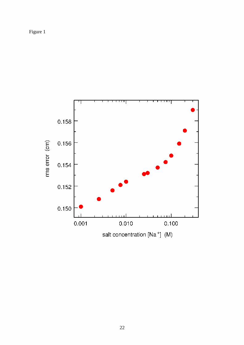
[Na+] ranging from 0.001 M to 0.3 M. Results are shown in Figs. 1 and 2. It is seen in Fig. 1

that the root mean square error between experimental and calculated absolute positions

actually remains essentially constant in the whole range 0.001-0.3 M. Furthermore,

examination of Fig. 2 indicates that the adjusted values of 0T and α vary logarithmically with

[Na+]. This is not really surprising because, as we already mentioned, the melting temperature

of a given sequence increases logarithmically with [Na+]. At last, it is seen in the top plot of

Fig. 2 that the adjusted value of rL varies between 100 and 140 base pairs, which agrees with

previously reported values [16,17].

Figs. 1 and 2 are however not sufficient to illustrate how broad the space of solutions

is, that is how widely each parameter can be varied while still preserving a very good

agreement between observed and calculated absolute positions. To get a better insight, we

12

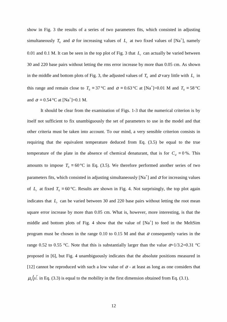
show in Fig. 3 the results of a series of two parameters fits, which consisted in adjusting

simultaneously 0T and α for increasing values of rL at two fixed values of [Na+], namely

0.01 and 0.1 M. It can be seen in the top plot of Fig. 3 that rL can actually be varied between

30 and 220 base pairs without letting the rms error increase by more than 0.05 cm. As shown

in the middle and bottom plots of Fig. 3, the adjusted values of 0T and α vary little with rL in

this range and remain close to 370 =T °C and 63.0=α °C at [Na+]=0.01 M and 580 =T °C

and 54.0=α °C at [Na+]=0.1 M.

It should be clear from the examination of Figs. 1-3 that the numerical criterion is by

itself not sufficient to fix unambiguously the set of parameters to use in the model and that

other criteria must be taken into account. To our mind, a very sensible criterion consists in

requiring that the equivalent temperature deduced from Eq. (3.5) be equal to the true

temperature of the plate in the absence of chemical denaturant, that is for 0=dC %. This

amounts to impose 600 =T °C in Eq. (3.5). We therefore performed another series of two

parameters fits, which consisted in adjusting simultaneously [Na+] and α for increasing values

of rL at fixed 600 =T °C. Results are shown in Fig. 4. Not surprisingly, the top plot again

indicates that rL can be varied between 30 and 220 base pairs without letting the root mean

square error increase by more than 0.05 cm. What is, however, more interesting, is that the

middle and bottom plots of Fig. 4 show that the value of [Na+] to feed in the MeltSim

program must be chosen in the range 0.10 to 0.15 M and that α consequently varies in the

range 0.52 to 0.55 °C. Note that this is substantially larger than the value α=1/3.2=0.31 °C

proposed in [6], but Fig. 4 unambiguously indicates that the absolute positions measured in

[12] cannot be reproduced with such a low value of α - at least as long as one considers that

( )s0µ in Eq. (3.3) is equal to the mobility in the first dimension obtained from Eq. (3.1).

13

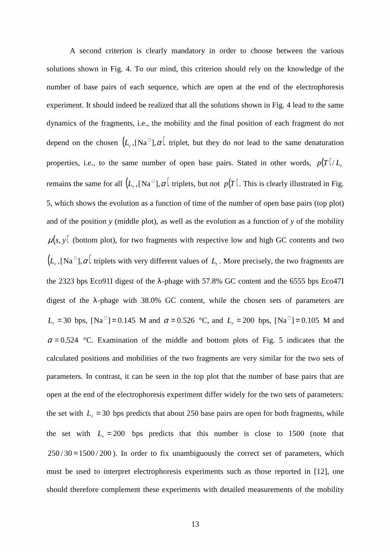
A second criterion is clearly mandatory in order to choose between the various

solutions shown in Fig. 4. To our mind, this criterion should rely on the knowledge of the

number of base pairs of each sequence, which are open at the end of the electrophoresis

experiment. It should indeed be realized that all the solutions shown in Fig. 4 lead to the same

dynamics of the fragments, i.e., the mobility and the final position of each fragment do not

depend on the chosen ( )α],Na[, +rL triplet, but they do not lead to the same denaturation

properties, i.e., to the same number of open base pairs. Stated in other words, ( ) rLTp /

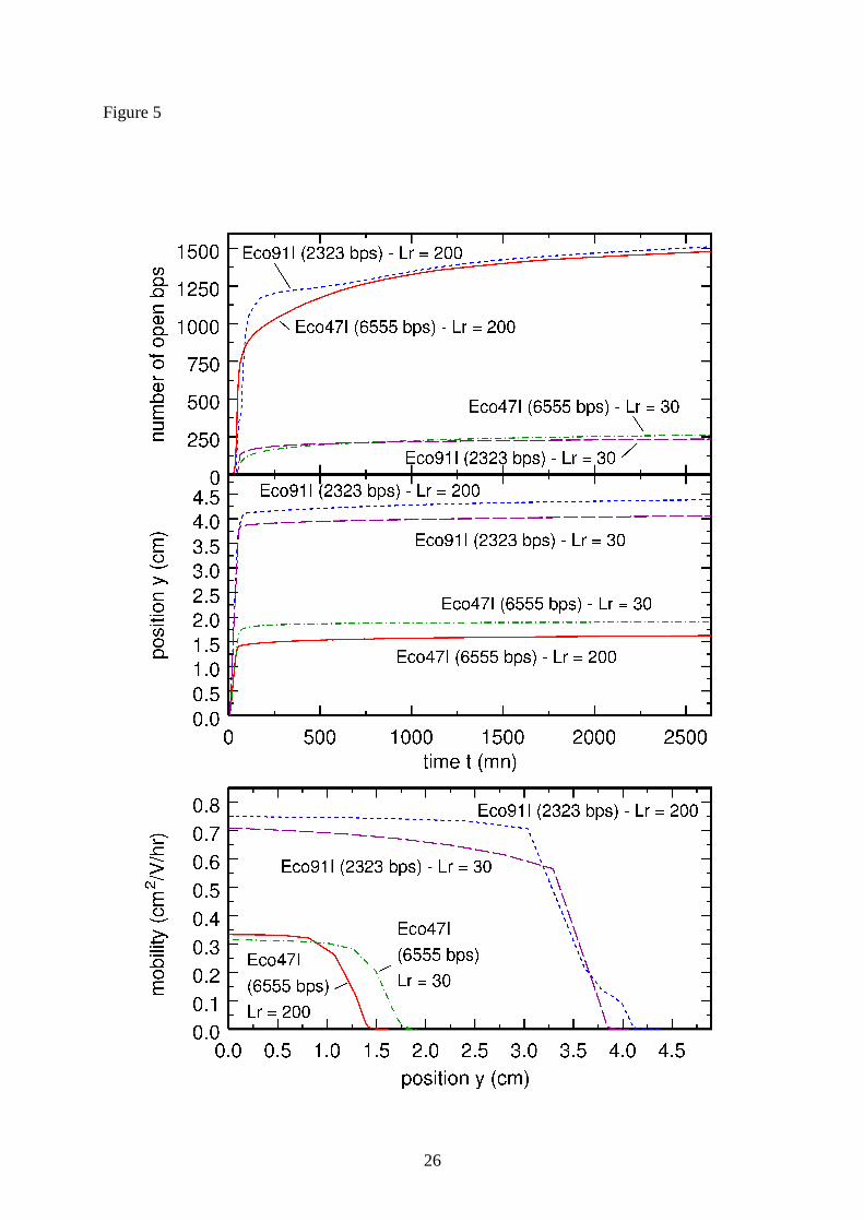
remains the same for all ( )α],Na[, +rL triplets, but not ( )Tp . This is clearly illustrated in Fig.

5, which shows the evolution as a function of time of the number of open base pairs (top plot)

and of the position y (middle plot), as well as the evolution as a function of y of the mobility

( )ys,µ (bottom plot), for two fragments with respective low and high GC contents and two

( )α],Na[, +rL triplets with very different values of rL . More precisely, the two fragments are

the 2323 bps Eco91I digest of the λ-phage with 57.8% GC content and the 6555 bps Eco47I

digest of the λ-phage with 38.0% GC content, while the chosen sets of parameters are

30=rL bps, 145.0]Na[ =+ M and 526.0=α °C, and 200=rL bps, 105.0]Na[ =+ M and

524.0=α °C. Examination of the middle and bottom plots of Fig. 5 indicates that the

calculated positions and mobilities of the two fragments are very similar for the two sets of

parameters. In contrast, it can be seen in the top plot that the number of base pairs that are

open at the end of the electrophoresis experiment differ widely for the two sets of parameters:

the set with 30=rL bps predicts that about 250 base pairs are open for both fragments, while

the set with 200=rL bps predicts that this number is close to 1500 (note that

200/150030/250 ≈ ). In order to fix unambiguously the correct set of parameters, which

must be used to interpret electrophoresis experiments such as those reported in [12], one

should therefore complement these experiments with detailed measurements of the mobility

14

of a few sequences, as in Fig. 4 of [16]. The positions of the bumps in the evolution of

mobility, which reflect the abrupt opening of large portions of the fragment, indeed reveal the

correct value of rL , and consequently also of ]Na[ + and α.

Since these additional data are not available for the experiments reported in [12], we

chose the set of parameters that leads to the smallest root mean square error, that is 100=rL

bps, 134.0]Na[ =+ M and 540.0=α °C, to compare calculated and experimental absolute

positions in the second dimension. Results are tabulated in the four last columns of Table 1. It

is stressed that the root mean square deviation between calculated and observed absolute

positions (0.15 cm) is almost twice smaller than the average experimental uncertainty (0.26

cm).

4 – Concluding remarks

In this paper, we have presented an (hopefully) exhaustive study of the numerical

issues associated with a model aimed at predicting the final absolute locations of DNA

fragments in 2D display experiments. In particular, we have shown that simple expressions

for the mobility of DNA fragments in both dimensions allow one to reproduce experimental

final absolute locations to better than experimental uncertainties. We have furthermore

pointed out that the results of 2D display experiments are not sufficient to determine the best

set of parameters for the modeling of fragments separation in the second dimension and that

additional detailed measurements of the mobility of a few sequences are necessary to achieve

this goal.

It was mentioned in the discussion at the end of [12], that the weakest part of this

model is probably Eq. (3.3), which expresses the mobility of a partially melted DNA

sequence as an exponentially decreasing function of the size of the melted regions, and that

15

the rL parameter should include some dependence on the properties of the gel (for example

its concentration and the size of the pores) and the studied DNA sequences (for example their

length, whether melting occurs at the extremities or inside the fragment, whether there is a

single melted region or several ones, etc). We made several attempts along these lines, but all

of them were unsuccessful. The reason for this is that the errors displayed in the last column

of Table 1 show no particular dependence on the length of the fragments, their GC content,

the distribution of the GC content inside the fragment and the number of melted regions at

each temperature. This, in turn, is probably due to the fact that experimental uncertainties,

which result essentially from the difficulty to control precisely the reproducibility of

experimental conditions, are almost twice as large as the root mean square deviation between

experimental and calculated positions. To our mind, it will not be possible (nor will it be

necessary !) to improve the model discussed here and in [12] as long as experimental

uncertainties will not be made substantially smaller than what can be achieved in today’s

experiments.

The authors declare no conflict of interest.

16

REFERENCES

[1] Fisher, S.G., Lerman, L.S., Cell 1979, 16, 191-200

[2] Fisher, S.G., Lerman, L.S., Proc. Natl. Acad. Sc. USA 1980, 77, 4420-4424

[3] Fisher, S.G., Lerman, L.S., Proc. Natl. Acad. Sc. USA 1983, 80, 1579-1583

[4] Viovy, J.L., Rev. Modern Phys. 2000, 72, 813-872

[5] Lerman, L.S., Fisher, S.G., Hurley, I. Silverstein, K., Lumelsky, N. Ann. Rev. Biophys.

Bioeng. 1984, 13, 399-423

[6] Lerman, L.S., Silverstein K., Methods Enzymol. 1987, 155, 482-501

[7] Malloff, C.A., Fernandez, R.C., Lam, W.L., J. Mol. Biol. 2001, 312, 1-5

[8] Malloff, C.A., Fernandez, R.C., Dullaghan, E.M., Stokes, R.W., Lam, W.L., Gene 2002,

293, 205-211

[9] Dullaghan, E.M., Malloff, C.A., Li, A.H., Lam, W.L., Stokes, R.W., Microbiology 2002,

148, 3111-3117

[10] Steger, G., Nucleic Acids Res. 1994, 22, 2760-2768

[11] Brossette, S., Wartell, R.M., Nucleic Acids Res. 1994, 22, 4321-4325

[12] Mercier, J.F., Kingsburry, C., Slater, G.W., Lafay, B., Electrophoresis 2008, 29, 1264-

1272

[13] Blake, R.D., Bizzaro, J.W., Blake, J.D., Day, G.R. et al, J. Bioinformatics 1999, 15, 370-

375

[14] Rill, R.L., Beheshti, A., Van Winkle, D.H., Electrophoresis 2002, 23, 2710-2719

[15] Van Winkle, D.H., Beheshti, A., Rill, R.L., Electrophoresis 2002, 23, 15-19

[16] Zhu, J., Wartell, R.M., Biochemistry 1997, 36, 15326-15335

[17] Wartell, R.M., Hosseini, S., Powell, S., Zhu, J., J. Chromatogr. A 1998, 806, 169-185

[18] Poland, D., Biopolymers 1974, 13, 1859-1871

17

[19] Fixman, M., Freire, J.J., Biopolymers 1977, 16, 2693-2704

[20] Blake, R.D., Delcourt, S.G., Nucleic Acids Res. 1998, 26, 3323-3332

[21] Meyers, R. M., Maniatis T., Lerman L. S., Methods Enzymol. 1987, 155, 501-527

18

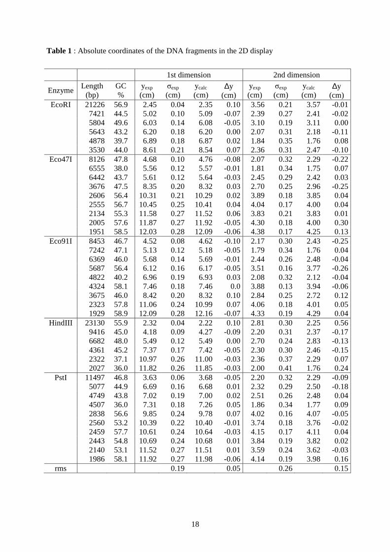
Table 1 : Absolute coordinates of the DNA fragments in the 2D display

1st dimension 2nd dimension

Enzyme Length

(bp) GC %

yexp (cm)

σexp (cm)

ycalc (cm)

∆y (cm)

yexp (cm)

σexp (cm)

ycalc (cm)

∆y (cm)

EcoRI 21226 56.9 2.45 0.04 2.35 0.10 3.56 0.21 3.57 -0.01 7421 44.5 5.02 0.10 5.09 -0.07 2.39 0.27 2.41 -0.02 5804 49.6 6.03 0.14 6.08 -0.05 3.10 0.19 3.11 0.00 5643 43.2 6.20 0.18 6.20 0.00 2.07 0.31 2.18 -0.11 4878 39.7 6.89 0.18 6.87 0.02 1.84 0.35 1.76 0.08 3530 44.0 8.61 0.21 8.54 0.07 2.36 0.31 2.47 -0.10

Eco47I 8126 47.8 4.68 0.10 4.76 -0.08 2.07 0.32 2.29 -0.22 6555 38.0 5.56 0.12 5.57 -0.01 1.81 0.34 1.75 0.07 6442 43.7 5.61 0.12 5.64 -0.03 2.45 0.29 2.42 0.03 3676 47.5 8.35 0.20 8.32 0.03 2.70 0.25 2.96 -0.25 2606 56.4 10.31 0.21 10.29 0.02 3.89 0.18 3.85 0.04 2555 56.7 10.45 0.25 10.41 0.04 4.04 0.17 4.00 0.04 2134 55.3 11.58 0.27 11.52 0.06 3.83 0.21 3.83 0.01 2005 57.6 11.87 0.27 11.92 -0.05 4.30 0.18 4.00 0.30 1951 58.5 12.03 0.28 12.09 -0.06 4.38 0.17 4.25 0.13

Eco91I 8453 46.7 4.52 0.08 4.62 -0.10 2.17 0.30 2.43 -0.25 7242 47.1 5.13 0.12 5.18 -0.05 1.79 0.34 1.76 0.04 6369 46.0 5.68 0.14 5.69 -0.01 2.44 0.26 2.48 -0.04 5687 56.4 6.12 0.16 6.17 -0.05 3.51 0.16 3.77 -0.26 4822 40.2 6.96 0.19 6.93 0.03 2.08 0.32 2.12 -0.04 4324 58.1 7.46 0.18 7.46 0.0 3.88 0.13 3.94 -0.06 3675 46.0 8.42 0.20 8.32 0.10 2.84 0.25 2.72 0.12 2323 57.8 11.06 0.24 10.99 0.07 4.06 0.18 4.01 0.05 1929 58.9 12.09 0.28 12.16 -0.07 4.33 0.19 4.29 0.04

HindIII 23130 55.9 2.32 0.04 2.22 0.10 2.81 0.30 2.25 0.56 9416 45.0 4.18 0.09 4.27 -0.09 2.20 0.31 2.37 -0.17 6682 48.0 5.49 0.12 5.49 0.00 2.70 0.24 2.83 -0.13 4361 45.2 7.37 0.17 7.42 -0.05 2.30 0.30 2.46 -0.15 2322 37.1 10.97 0.26 11.00 -0.03 2.36 0.37 2.29 0.07 2027 36.0 11.82 0.26 11.85 -0.03 2.00 0.41 1.76 0.24

PstI 11497 46.8 3.63 0.06 3.68 -0.05 2.20 0.32 2.29 -0.09 5077 44.9 6.69 0.16 6.68 0.01 2.32 0.29 2.50 -0.18 4749 43.8 7.02 0.19 7.00 0.02 2.51 0.26 2.48 0.04 4507 36.0 7.31 0.18 7.26 0.05 1.86 0.34 1.77 0.09 2838 56.6 9.85 0.24 9.78 0.07 4.02 0.16 4.07 -0.05 2560 53.2 10.39 0.22 10.40 -0.01 3.74 0.18 3.76 -0.02 2459 57.7 10.61 0.24 10.64 -0.03 4.15 0.17 4.11 0.04 2443 54.8 10.69 0.24 10.68 0.01 3.84 0.19 3.82 0.02 2140 53.1 11.52 0.27 11.51 0.01 3.59 0.24 3.62 -0.03 1986 58.1 11.92 0.27 11.98 -0.06 4.14 0.19 3.98 0.16

rms 0.19 0.05 0.26 0.15

19

The table indicates the size (in base pairs) of each fragment, its GC content (in %), and, for

each dimension, the experimental absolute position (yexp, in cm) averaged over three

experiments, the experimental uncertainty (σexp, in cm), the calculated absolute position (ycalc,

in cm) and the error (∆y=yexp-ycalc, in cm). Absolute positions in the first dimension were

obtained with the expression of mobility in Eq. (3.1) and parameters 41017.0 −×=Lµ cm2/(V

s), 41053.4 −×=Sµ cm2/(V s) and 41200=m . Absolute positions in the second dimension

were obtained with the expression of mobility in Eq. (3.3), the expression of equivalent

temperature in Eq. (3.5), and parameters 100=rL bps, 134.0]Na[ =+ M, 600 =T °C and

540.0=α °C.

20

FIGURE CAPTIONS

Figure 1 : Root mean square deviations (expressed in cm) between experimental and

calculated absolute positions along the second dimension (DGGE experiments) for the 40

DNA sequences listed in Table 1. The three parameters rL , 0T and α were adjusted

simultaneously for each fixed value of the salinity [Na+].

Figure 2 : Adjusted values of rL (top plot, units of base pairs), 0T (middle plot, units of °C),

and α (bottom plot, units of °C), as a function of the fixed salinity [Na+].

Figure 3 : Results of a series of two parameters fits, which consisted in adjusting

simultaneously 0T and α for increasing values of rL at two fixed values of [Na+] (0.01 and

0.1 M). The top plot shows the root mean square error (expressed in cm) between

experimental and calculated absolute positions along the second dimension (DGGE

experiments) for the 40 DNA sequences listed in Table 1. The middle plot shows the

evolution of 0T (expressed in °C) and the bottom plot the evolution of α (expressed in °C).

Figure 4 : Results of a series of two parameters fits, which consisted in adjusting

simultaneously [Na+] and α for increasing values of rL at fixed 600 =T °C. The top plot

shows the root mean square error (expressed in cm) between experimental and calculated

absolute positions along the second dimension (DGGE experiments) for the 40 DNA

sequences listed in Table 1. The middle plot shows the evolution of [Na+] (expressed in M)

and the bottom plot the evolution of α (expressed in °C).

21

Figure 5 : Evolution as a function of time of the number of open base pairs (top plot) and of

the position y (middle plot), and evolution as a function of y of the mobility ( )ys,µ (bottom

plot), for two different fragments and two different sets of parameters. The two fragments are

the 2323 bps Eco91I digest with 57.8% GC content and the 6555 bps Eco47I digest with

38.0% GC content. The two sets of parameters are 30=rL bps, 145.0]Na[ =+ M and

526.0=α °C, and 200=rL bps, 105.0]Na[ =+ M and 524.0=α °C. 600 =T °C for both

sets.

22

Figure 1

23

Figure 2

24

Figure 3

25

Figure 4

26

Figure 5