ana paula pereira peixoto search for tz production via ... · nome: ana paula pereira peixoto...
TRANSCRIPT

CER
N-T
HES
IS-2
016-
313
12/0
9/20
16
Ana Paula Pereira Peixoto
Search for tZ production via Flavour Changing
Neutral Currents with the ATLAS experiment
at the LHC
Agosto de 2016Um
inho |
2016
Ana P
aula
Pere
ira P
eix
oto
Se
arc
h f
or
tZ p
rod
ucti
on
via
Fla
vo
ur
Ch
an
gin
g N
eu
tra
l C
urr
en
ts
wit
h t
he
AT
LA
S e
xp
eri
me
nt
at
the
LH
C
Universidade do Minho
Escola de Ciências


Ana Paula Pereira Peixoto
Search for tZ production via Flavour Changing
Neutral Currents with the ATLAS experiment
at the LHC
Agosto de 2016
Dissertação de MestradoMestrado em Física - Física Aplicada
Trabalho efetuado sob a orientação do
Professor Doutor Nuno Filipe da Silva Fernandes de Castro
Universidade do Minho
Escola de Ciências

Declaracao
Nome: Ana Paula Pereira Peixoto
E-mail: [email protected]
Telefone:+351969233066
Numero de Cartao de Cidadao:13630865
Tıtulo da Tese: Search for tZ production via Flavour Changing Neutral Currents
with the ATLAS experiment at the LHC
Orientador: Doutor Nuno Filipe da Silva Fernandes de Castro
Ano de Conclusao:2016
Designacao do Mestrado: Mestrado em Fısica Aplicada
E AUTORIZADA A REPRODUCAO INTEGRAL DESTA TESE APENAS PARA
EFEITOS DE INVESTIGACAO, MEDIANTE DECLARACAO ESCRITA DO
INTERESSADO, QUE A TAL SE COMPROMETE;
Universidade do Minho, 29/08/2016
Assinatura:
Ana Paula Pereira Peixoto
Search for tZ production via Flavour ChangingNeutral Currents with the ATLAS experiment
at the LHC
Tese de Mestrado
Mestrado em Fısica - Fısica Aplicada
Trabalho efectuado sob orientacao do
Professor Doutor Nuno Filipe da Silva Fernandes de Castro
Agosto de 2016


Acknowledgedments
This thesis would not be possible without the support of many people. I would
like to gratefully acknowledge all of them, in particular the people that supervised
my work, those with whom I have worked and those who shared their knowledge
with me.
First of all, I would like to express my gratitude to Dr. Nuno Castro for many
reasons but more importantly for being a very supportive and, at same time,
exigent advisor. Thanks for all you taught me and for the opportunities you gave
me.
I also have to thank the Humboldt University (Berlin, Germany) for letting me use
their analysis code as well as the cluster to run the analysis presented in this thesis.
A special thanks to the Humboldt University group involved in this work composed
by Oliver Kind, Thomas Lohse, Sebastian Mergelmeyer and Soren Stamm. They
made possible a big part of the work presented here through their expert advices
and their support from the first minute of our collaboration. I would like to also
thank for their hospitality during my stay in Berlin. I have to acknowledge, in
particular, Oliver Kind and Sebastian Mergelmeyer for always being available to
help me and for everything I learned with them.
I thank the LIP-Minho team, specially my close colleagues Juan Pedro Araque,
Tiago Vale and Jose Correia for all the help they gave me and for the moments
we spent during the last year.
I would like to thank the whole LIP team for their support with a special thanks
to the Portuguese ATLAS group. I also have to thank all the people in the Single
Top subgroup in ATLAS for all the important advices to the development of this
iii
iv
analysis.
A special word of gratitude goes to my Physics and Chemistry teacher Sonia Torres
for introducing me to the physics world and for made me believe in my dream of
being a physicist.
The most important thanks go to all my family specially to my mother Manuela
and my father Carlos for all their patience and emotional support. Thanks for the
motivation and love you give me every day. Finally, I want to thank Tiago who
always understands and helps me no matter what. Thank you for being always by
my side.
I thank LIP (Laboratorio de Instrumentacao e Fısica Experimental de Partıculas),
FCT/MEC (Fundacao Ciencia e Tecnologia / Ministerio da Educacao e da Ciencia),
FEDER (Fundo Europeu de Desenvolvimento Regional) for funding my activi-
ties this past year, as established by the partnership PT2020 partnership with
COMPETE2020 (Autoridade de Gestao do Programa Operacional Competitivi-
dade e Internacionalizacao), by providing me with a research scholarship (Refer-
ence LIP/BI-26/2015).
Resumo
A presente dissertacao tem como objectivo a pesquisa da producao de eventos
tZ atraves de processos de mudanca de sabor por correntes neutras recorrendo a
uma analise de dados colectados pelo detector ATLAS do Large Hadron Collider
localizado no CERN. Os processos de mudanca de sabor por correntes neutras sao
muito raros no Modelo Padrao da Fısica de Partıculas, sendo ausentes a tree-level e
extremamente suprimidos a loop-level. No entanto, estes processos tem uma maior
probabilidade de ocorrer em varios modelos para alem do Modelo Padrao.
Neste trabalho e estudada a producao de um quark top e de um bosao Z atraves de
processos de mudanca de sabor por correntes neutras numa topologia trileptonica.
O estado final desta pesquisa consiste num par de leptoes de carga oposta e sabor
identico com uma massa compatıvel com o decaimento de um bosao Z, um leptao
carregado em conjunto com um leptao neutro provenientes do decaimento de um
quark top e finalmente um jacto proveniente de um quark bottom (b-tagged jet).
Os dados analisados, relativos a colisoes protao-protao a uma energia de centro de
massa de√s = 13 TeV, foram obtidos no perıodo de Julho a Novembro de 2015
correspondendo a uma luminosidade integrada de 3.21 fb−1.
Um estudo complementar de possıveis variaveis discriminantes e apresentado.
Atraves deste estudo, sao obtidos limites superiores esperados com um nıvel de
confianca de 95% na seccao eficaz de producao deste processo. Estes limites sao
interpretados em termos do acoplamento tZq e da fraccao de decaimento t → qZ.
v

vi
Abstract
The subject of the present dissertation is the search for tZ event production by
Flavour Changing Neutral Currents (FCNC) through the analysis of data collected
by the ATLAS detector of the Large Hadron Collider located in CERN. The FCNC
processes are very rare in the Standard Model of Particle Physics since they are
not allowed at tree-level and extremely suppressed at loop-level. However, this
processes have a higher probability to occur in several models beyond the Standard
Model.
In this thesis, a search for the production of a top quark and a boson Z via FCNC
in a trileptonic topology is discussed. The final state of the tZ production consists
in a pair of leptons with opposite sign and same flavour having a mass compatible
with the decay of a Z boson, a charged lepton and a neutral lepton classified as
coming from the decay of a top quark and finally a jet coming from a bottom
quark (b-tagged jet). The analyzed data coming from proton-proton collisions at
the centre-of-mass energy of√s = 13 TeV was collected in the data-taking period
between July and November of 2015 corresponding to an integrated luminosity of
3.21 fb−1.
A complementary study of possible discriminant variables is presented. Through
this study, expected upper limits at 95% confidence level on the cross-section of
tZ production via FCNC were obtained. An interpretation of these limits in terms
of branching ratios for t → qZ and the tZq coupling is also presented.
vii

viii

Contents
1 Introduction 1
2 The Standard Model of particle physics and beyond 3
2.1 The Standard Model of particle physics . . . . . . . . . . . . . . . . 3
2.1.1 Quantum electrodynamics . . . . . . . . . . . . . . . . . . . 6
2.1.2 Quantum chromodynamics . . . . . . . . . . . . . . . . . . . 7
2.1.3 Electroweak theory . . . . . . . . . . . . . . . . . . . . . . . 9
2.1.4 The Brout-Englert-Higgs mechanism . . . . . . . . . . . . . 10
2.2 Top quark physics . . . . . . . . . . . . . . . . . . . . . . . . . . . . 13
2.3 Top quark FCNC interactions . . . . . . . . . . . . . . . . . . . . . 15
3 Experimental Setup 19
3.1 CERN . . . . . . . . . . . . . . . . . . . . . . . . . . . . . . . . . . 19
3.2 The Large Hadron Collider . . . . . . . . . . . . . . . . . . . . . . . 20
3.3 The ATLAS detector . . . . . . . . . . . . . . . . . . . . . . . . . . 22
3.3.1 Inner detector . . . . . . . . . . . . . . . . . . . . . . . . . . 23
3.3.2 Calorimeters . . . . . . . . . . . . . . . . . . . . . . . . . . . 25
3.3.3 Muon spectrometer . . . . . . . . . . . . . . . . . . . . . . . 26
3.3.4 Magnet system . . . . . . . . . . . . . . . . . . . . . . . . . 28
3.3.5 Trigger and data acquisition system . . . . . . . . . . . . . . 28
3.3.6 Worldwide LHC Computer GRID . . . . . . . . . . . . . . . 29
4 Event analysis 33
4.1 Data sample and triggers . . . . . . . . . . . . . . . . . . . . . . . . 33
ix

x
4.2 Objects definition . . . . . . . . . . . . . . . . . . . . . . . . . . . . 34
4.3 Analysis strategy . . . . . . . . . . . . . . . . . . . . . . . . . . . . 37
4.4 Signal modeling . . . . . . . . . . . . . . . . . . . . . . . . . . . . . 40
4.5 Background modeling . . . . . . . . . . . . . . . . . . . . . . . . . . 40
4.6 Signal region definition . . . . . . . . . . . . . . . . . . . . . . . . . 42
4.7 Comparison between data and prediction . . . . . . . . . . . . . . . 46
4.7.1 Validation regions . . . . . . . . . . . . . . . . . . . . . . . . 46
4.8 Systematic uncertainties . . . . . . . . . . . . . . . . . . . . . . . . 61
4.9 Discriminant variables . . . . . . . . . . . . . . . . . . . . . . . . . 62
5 Limits 71
5.1 The CLs method . . . . . . . . . . . . . . . . . . . . . . . . . . . . 71
5.2 Limits on the tZ production . . . . . . . . . . . . . . . . . . . . . . 73
6 Conclusions 77

List of Figures
2.2.1 Leading order Feynman diagrams corresponding to the top quark
pair production through quark anti-quark annihilation and gluon
fusion [22]. . . . . . . . . . . . . . . . . . . . . . . . . . . . . . . . . 14
2.2.2 Feynman diagrams for the single top quark production at leading
order. . . . . . . . . . . . . . . . . . . . . . . . . . . . . . . . . . . 14
2.2.3 Summary of ATLAS and CMS measurements of the single top pro-
duction cross-sections in various channels as a function of the center
of mass energy [24, 25, 26, 27, 28, 29, 30, 31, 32, 33, 34, 35, 36, 37,
38, 39, 40, 41, 42, 43, 44]. . . . . . . . . . . . . . . . . . . . . . . . 15
2.3.1 Summary of the current 95% CL observed limits on the branching
ratios of the top quark decays via FCNC to a charm quark (left)
and to an up quark (right) along with a neutral boson [59]. . . . . . 18
3.1.1 Schematic view of the CERN accelerator complex.[62] . . . . . . . . 20
3.3.1 Representation of the ATLAS detector showing the different subsystems.[61] 22
3.3.2 Representation of the ATLAS inner detector. The pixel detectors
refers to the Insertable B-Layer and the Pixel Detector. [73] . . . . 24
3.3.3 Open view of the ATLAS calorimeter system.[74] . . . . . . . . . . 26
3.3.4 Representation of the ATLAS muon spectrometer.[75] . . . . . . . . 27
3.3.5 The total integrated luminosity delivered in the year of 2015 as a
function of time [76]. . . . . . . . . . . . . . . . . . . . . . . . . . . 29
xi

xii
3.3.6 Representation of the structure of the tiers 0, 1 and 2. The various
locations of the thirteen computer centres of tier 1 can also be found
[78]. . . . . . . . . . . . . . . . . . . . . . . . . . . . . . . . . . . . 31
4.2.1 The efficiency to tag b, c and light-flavour jets for the MV2c20 tagger
with the 77% working point. Efficiencies are shown as a function of
the jet pT and |η| [92, 93]. . . . . . . . . . . . . . . . . . . . . . . . 36
4.3.1 Distributions concerning the leptons after require events containing
exactly one jet. . . . . . . . . . . . . . . . . . . . . . . . . . . . . . 38
4.3.2 Distributions of relevant variables after require exactly one jet and
three leptons. . . . . . . . . . . . . . . . . . . . . . . . . . . . . . . 39
4.6.1 Signal region distributions before and after the b-tagged jet require-
ment. . . . . . . . . . . . . . . . . . . . . . . . . . . . . . . . . . . . 43
4.6.2 Signal region distributions before and after the b-tagged jet require-
ment. . . . . . . . . . . . . . . . . . . . . . . . . . . . . . . . . . . . 44
4.7.1 Z+jets dilepton control region distributions before and after the
b-tagged jet requirement. . . . . . . . . . . . . . . . . . . . . . . . . 48
4.7.2 Z+jets dilepton control region distributions of b-tagged jet multi-
plicity before and after the final requirement. . . . . . . . . . . . . . 49
4.7.3 Z+jets trilepton control region relevant distributions before and
after the b-tagged jet requirement. . . . . . . . . . . . . . . . . . . . 51
4.7.4 Z+jets trilepton control region distributions of b-tagged jet multi-
plicity before and after the b-tagged jet requirement. . . . . . . . . 52
4.7.5 tt control region distributions before and after the b-tagged jet re-
quirement. . . . . . . . . . . . . . . . . . . . . . . . . . . . . . . . . 53
4.7.6WZ Diboson control region distributions after the selection criteria. 57
4.7.7 tZj control region distributions before and after the b-tagged jet
requirement. . . . . . . . . . . . . . . . . . . . . . . . . . . . . . . . 59
4.9.1 Two dimensional distributions for different backgrounds shown as
a function of the Z boson candidate pT and the reconstructed top
quark mass and the transverse mass of the W boson. . . . . . . . . 63

xiii
4.9.2 Two dimensional distributions for the Z+jets background and sig-
nal, shown as function of the Z boson candidate pT and the recon-
structed top quark mass and the transverse mass of the W boson. . 64
4.9.3 Relevant distributions for the signal region with the added cut on
the transverse mass of the W boson. . . . . . . . . . . . . . . . . . 66
4.9.4 Relevant distributions of the signal region with the added cut on
the reconstructed top quark mass. . . . . . . . . . . . . . . . . . . . 69
5.2.1 The pull plot for the systematics studied in this analysis and their
correlation with the signal. . . . . . . . . . . . . . . . . . . . . . . . 75
5.2.2 Expected upper limits at 95% CL for the anomalous couplingKLut/Λ
considering the expected upper limits of the cross-sections for a lu-
minosity of 3.21 fb−1 and 30 fb−1 and the theoretical prediction. . . 76
6.0.1 Luminosity per year for the different centre-of-mass energy at the
LHC [100]. . . . . . . . . . . . . . . . . . . . . . . . . . . . . . . . . 78

xiv

List of Tables
2.1.1 The fundamental fermions of the Standard Model and their mass
and charge according to the Particle data Group [5]. . . . . . . . . . 5
2.1.2 The interactions in the Standard Model and their mediating gauge
bosons with the mass and charge according to the Particle data
Group [5]. . . . . . . . . . . . . . . . . . . . . . . . . . . . . . . . . 6
2.3.1 The theoretical values for the branching ratios of FCNC top decays
predicted by the Standard Model, the quark-singlet model (QS), the
two Higgs doublet model (2HDM), the flavour-conserving two Higgs
doublet model (FC 2HDM), the minimal supersymmetric model
(MSSM) and SUSY with R parity violation ( 6R SUSY) [50]. . . . . . 16
2.3.2 Summary of the 95% CL observed limits on the branching ratios
along with the production mode, the luminosity and the centre-of-
mass energy for the different searches performed by the ATLAS and
the CMS collaboration. . . . . . . . . . . . . . . . . . . . . . . . . . 17
4.2.1 Operating points for the MV2c20 b-tagging algorithm including the
c-jet and light-jets rejection rates [91]. . . . . . . . . . . . . . . . . 36
4.5.1 Background MC samples with the corresponding cross-sections and
generators used in the analysis presented in this thesis. . . . . . . . 41
4.6.1 Signal region event yields after the selection criteria. The uncer-
tainties presented corresponds only to the statistical errors. . . . . . 45
4.7.1 Selection criteria used to define the considered control regions. . . . 46
xv

xvi
4.7.2 Z+jets dilepton control region event yields after the selection crite-
ria. The uncertainties presented corresponds only to the statistical
errors. . . . . . . . . . . . . . . . . . . . . . . . . . . . . . . . . . . 49
4.7.3 Z+jets trilepton control region event yields after the selection crite-
ria. The uncertainties presented corresponds only to the statistical
errors. . . . . . . . . . . . . . . . . . . . . . . . . . . . . . . . . . . 52
4.7.4 tt control region event yields after the selection criteria. The uncer-
tainties presented corresponds only to the statistical errors. . . . . . 55
4.7.5WZ Diboson control region event yields after the selection criteria.
The uncertainties presented corresponds only to the statistical errors. 58
4.7.6 tZj control region event yields after the selection criteria. The
uncertainties presented corresponds only to the statistical errors. . . 60
4.9.1 Definition of distinct signal region selections in order to separate
background for signal. A cut on the transverse mass of W boson or
in the reconstructed top quark mass are added to the signal region
selection. . . . . . . . . . . . . . . . . . . . . . . . . . . . . . . . . . 65
4.9.2 Event yields for the signal region selection with a cut on the trans-
verse mass of the reconstructed W boson. The uncertainties pre-
sented corresponds only to the statistical errors. . . . . . . . . . . . 68
4.9.3 Event yields for the signal region selection with a cut on the recon-
structed top quark mass. The uncertainties presented corresponds
only to the statistical errors. . . . . . . . . . . . . . . . . . . . . . . 70

List of Acronyms
ALICE A Large Ion Collider Experiment
ATLAS A Toroidal LHC ApparatuS
BSM Beyond the Standard Model
CKM Cabibbo-Kobayashi-Maskawa
CL Confidence Level
CMS Compact Muon Solenoid
CERN Conseil Europeen pour la Recherche Nucleaire
FCNC Flavour Changing Neutral Currents
LHC Large Hadron Collider
LO Leading Order
MC Monte Carlo
OSSF Opposite-Sign Same-Flavour
xvii

xviii
SM Standard Model of Particle Physics
SPS Super Proton Synchroton
PS Proton Synchroton
QCD Quantum Chromodynamics
QED Quantum Electrodynamics
WLCG Worldwide LHC Computer GRID

Chapter 1
Introduction
The Standard Model of particle physics (SM), developed in the 1960’s [1], is the
theoretical framework that so far best describes the nature of the subatomic world.
This model has been severely tested and has been very successful in the description
of the experimental observations. However, this theory cannot explain phenomena
like the neutrinos masses or the dark matter and dark energy. Several models
were presented to extend the SM since is thought that it is not the most complete
theory of particle physics.
Discovered in 1995 [2, 3], the top quark is the heaviest particle in the SM and
decays almost all the times to a W boson and a b-quark. The top quark can decay
also through a neutral current. Within the SM, the Flavour Changing Neutral
Currents (FCNC) processes are forbidden at tree level due to the GIM mechanism
[4] and is suppressed at higher orders because of unitary of the CKM matrix.
In extensions of the SM it is possible having FCNC processes at tree level and
loop level where enhancements of the FCNC branching ratios were predicted. The
study of the top FCNCs interactions can be performed in two modes: one in the
t production along with a Z boson, Higgs boson or a photon (γ) and another in
the tt decays.
In this thesis, a search for the production of a single top quark in association
with a Z boson is considered. The goal of this thesis is to perform an analysis
comparing data events with an integrated luminosity of 3.21 fb−1 recorded with
1
Chapter 1: Introduction 2
a centre-of-mass energy of√s= 13 TeV at the ATLAS detector with simulated
events for the signal region and for the different control regions. The study of
possible discriminant variables for the signal region is also performed, presenting
expected limits for the branching ratio of the tZ production via FCNC processes.
In Chapter 2 a review of the SM and an introduction to the FCNC processes are
presented. Chapter 3 is composed by a presentation of the CERN and a review of
the LHC and of the ATLAS detector. A description of the analysis used to study
the signal region and the different control regions is made in Chapter 4. Expected
upper limits at 95% confidence level (CL) on the cross-section for the process pp
→ tZ were obtained in the Run-2 of the LHC at√s= 13 TeV with an integrated
luminosity of 3.21 fb−1 and 30 fb−1 are presented in Chapter 5. These limits were
also interpreted as limits on the coupling tZq and the branching ratio of the decay
t → qZ.

Chapter 2
The Standard Model of particle
physics and beyond
The SM is the theoretical framework that so far better describes the subatomic
world. Developed in the 1960’s [1], it has been tested and successful in describing
the experimental observations. This chapter briefly introduces the structure of the
SM and the FCNC interactions.
2.1 The Standard Model of particle physics
The matter is made from atoms which are made from electrons and nuclei. The
atomic nucleus is made of neutrons and protons and both of them are made of
elementary particles named quarks. The elementary particles interact via four
fundamental forces in nature: strong force, weak force, electromagnetic force and
gravitational force.
The strong interaction is responsible for the stability of the atomic nuclei by pre-
venting them from fragmenting as a result of the electric repulsion of the protons
and is a very short range force (typically around 10−15 m). The weak force is
responsible for the beta decay of unstable atoms and acts at very short distances
(typically around 10−18 m). The electromagnetic interaction acts over an infinite
range and is responsible for the interaction between electric charged particles. The
3

Section 2.1: The Standard Model of particle physics 4
electromagnetic force is well defined through the Maxwell equations. The gravita-
tional force is an interaction between massive objects with an infinite range. The
strong, weak and electromagnetic forces are the interactions included in the SM
of particle physics.
Based on relativistic quantum field theory, the SM describes the interactions be-
tween the elementary particles. This model assumes that matter is made from
elementary point-like particles with spin 1/2 called fermions. The interactions be-
tween the fermions are mediated by spin 1 particles called bosons. There are two
types of fermions: quarks and leptons. The leptons are divided in the electrically
charged with the fundamental charge of e = −1.6 × 10⁻¹⁹ C and the electrically
neutral particles called neutrinos (ν). In the other hand, the quarks carry frac-
tional charge which can be +2/3 |e| or - 1/3 |e|. The quarks carry also another
quantum number which is the colour charge. This charge is of three different types:
red, green or blue. Another characteristic of the fermions is that every particle has
an associated antiparticle with the same mass but carrying the opposite charge to
its corresponding particle.
The fermions are grouped into three generations. The difference between the
generations is the flavour, i.e. the fermion type, and the mass of the particles,
remaining the other corresponding quantum numbers. Each generation is defined
by two doublets, one in the lepton family and one in the quark family. The doublet
from the lepton family contains a charged lepton and his partner neutrino. The
doublet from the quark family contains a quark with a charge of + 2/3 |e| anda quark with a charge of - 1/3 |e|. There are three lepton doublets: the electron
(e) with his partner electron neutrino (νe), the muon (µ) with his partner muon
neutrino (νµ) and the tau (τ) with his partner tau neutrino (ντ ). The electron
doublet, the muon doublet and the tau doublet correspond to the first, second and
third generation of leptons, respectively.
There are three quark doublets: the up quark (u) with the down quark (d), the
charm quark (c) with the strange quark (s) and the top quark (t) with the bottom
quark (b). The up doublet, the charm doublet and the top doublet correspond
to the first, second and third generation of quarks, respectively. The elementary

5 Section 2.1: The Standard Model of particle physics
particles in the SM are listed in Table 2.1.1.
Generation Symbol Name Mass Electric charge (|e|)
Quarks
1stu Up 2.3 MeV +2/3
d Down 4.8 MeV -1/3
2ndc Charm 1.3 GeV +2/3
s Strange 95 MeV -1/3
3rdt Top 173.5 GeV +2/3
b Bottom 4.6 GeV -1/3
Leptons
1ste Electron 0.5 MeV -1
νe Electron Neutrino < 2 eV 0
2ndµ Muon 105.7 MeV -1
νµ Muon Neutrino < 2 eV 0
3rdτ Tau 1.8 GeV -1
ντ Tau Neutrino < 2 eV 0
Table 2.1.1: The fundamental fermions of the Standard Model and their mass and
charge according to the Particle data Group [5].
The bosonic sector is responsible for the interactions described in the SM. The
electromagnetic force carrier is the photon (γ). The photon is a massless parti-
cle and electrically neutral. The weak force carriers are the W± and Z bosons.
Before their discovery, the theory predicted that they should be massive. The Z
boson is electrically neutral and theW± bosons have positive and negative electric

Section 2.1: The Standard Model of particle physics 6
charge, respectively. The strong force carriers are the gluons (g) which are massless
particles with no electric charge. Since gluons carry colour charge with eight com-
binations, they interact among themselves and only couple to the strong charged
particles. Consequently, only quarks can participate in the strong interaction.
The gauge bosons of the three forces and their characteristics are summarized in
Table 2.1.2.
Beside this twelve gauge bosons, the SM contains one scalar boson, the Higgs
boson.
Interaction Mediator Mass (GeV) Electric Charge (|e|)
Strong Gluon × 8 (g) 0 0
Electromagnetic Photon (γ) 0 0
WeakZ 91.19 0
W± 80.39 ±1
Table 2.1.2: The interactions in the Standard Model and their mediating gauge
bosons with the mass and charge according to the Particle data Group [5].
2.1.1 Quantum electrodynamics
The classical theory of electromagnetic interactions is well known through the
Maxwell equations of the nineteenth century. The theory of Quantum Electrody-
namics (QED) unified electrodynamics and quantum mechanics providing a quan-
tum field theory based on the gauge invariance of electrodynamics. The QED
theory describes the interactions between electrically charged particles mediated
by a quantized electromagnetic field.
The free spin 1/2 particles are described in the Dirac Lagrangian
LDirac = ψ(iγµ∂µ −m)ψ (2.1.1)
where ψ corresponds to γ0ψ†, γµ (µ=1,2,3,4) corresponds to the Dirac matrices,
m is the fermion mass and ψ is the Dirac field. The Dirac matrices satisfy the

7 Section 2.1: The Standard Model of particle physics
following relations
γµ, γν = γµγν + γνγµ = 2gµν where gµν ≡ Metric tensor, (2.1.2)
γ5 = γ5 = iγ1γ2γ3γ4,
σµν =i
2[γµ, γν ] =
i
2(γµγν − γνγµ).
However, this Lagrangian is not invariant under a local U(1) gauge transformation
of the form
ψ −→ e−ieα(x)ψ and ψ −→ eieα(x)ψ (2.1.3)
where e is in units of the electric charge of the proton and α is a real number. With
this transformation the Dirac Lagrangian acquires an additional term of ψeγµ∂µψ.
To obtain a U(1) invariant Lagrangian, another term with the expression ψeγµAµψ
is added, where Aµ is the four-potential of the electromagnetic field.
Adding this term and the free field dynamics, described by the Maxwell equation,
the QED Lagrangian can be obtained:
LQED = −1
4F µνFµν + ψ[iγµ(∂µ − eAµ) +m]ψ (2.1.4)
where F µν = ∂µAν − ∂νAµ is the electromagnetic field tensor. Requiring local
phase invariance under U(1) applied to free Dirac Lagrangian, it is generated all
of electrodynamics and introduced a massless field which can be interpreted as the
photon.
2.1.2 Quantum chromodynamics
The interactions between quarks and gluons are described by a quantum field
theory called Quantum Chromodynamics (QCD) [6]. Analogous to the electric
charge in QED, each quark has an internal degree of freedom known as colour.
This new quantum number was introduced to explain how bound stated of three
identical quarks can exist and not violate the Pauli exclusion principle. The quark
colour state could be red (R), green (G) or blue (B). In this theory, the quarks
interact with each other through a gluon exchange. The gluon exchange changes
the colour state of the interacting quarks. The gluons also interact with each other
implying that the gluons are also colour carriers.

Section 2.1: The Standard Model of particle physics 8
The QCD theory is based on the gauge group SU(3) where exists three dimensions
and each dimension is a colour (R, G and B). The number of gluons is eight since
SU(3) has eight generators where each generator represents a colour exchange and
a gauge boson (gluon) in colour space. The generators of SU(3) are written as
ta =1
2λa (2.1.5)
where λa with a =1,2,...,8 corresponds to the Gell-Mann matrices. Each quark
flavour consists in a triplet of fields represented as
q =
qR
qG
qB
(2.1.6)
where each of this fields is a Dirac spinor associated to a colour state.
The QCD Lagrangian is
LQCD = q(iγµDµ −m)q − 1
4Ga
µνGµνa (2.1.7)
with the covariant derivative Dµ = ∂µ + igstaGaµ and the strength field tensor
defined by
Gaµν = ∂µG
aν − ∂νG
aµ − gsf
abcGbµG
cν (2.1.8)
where Gaµ are the gluon fields, gs is the QCD gauge coupling constant and fabc
are the structure constant of SU(3)c defined by the commutation relation [ta, tb] =
ifabctc.
The QCD theory has been very successful in the description of the interactions
binding quarks to hadrons. However, there are two important characteristics of this
theory: asymptotic freedom and confinement [7, 8]. Asymptotic freedom means
that at very high energies and short distances quarks and gluons interact weakly
with each other allowing the computation of observables using the perturbation
theory. Confinement means that at very low energy scales which corresponds to
large distances, when we try to separate quarks, the energy of the gluon field in-
creases, creating quark and anti-quark pairs and, consequently, free quarks cannot
exist.

9 Section 2.1: The Standard Model of particle physics
2.1.3 Electroweak theory
Proposed by Glashow, Salam and Weinberg [9, 10, 11], the electroweak theory is a
unified theory of electroweak interactions which describe the weak and electromag-
netic forces from a single gauge group SU(2)L ⊗ U(1)Y where Y corresponds to
the weak hypercharge. The weak hypercharge is given by the Gell-Mann-Nishijima
relation Y = 2 (Q - T3) where T3 is the third component of the weak isospin op-
erator T = σi/2 (i=1,2,3) with σi corresponding to the three Pauli matrices and
Q is the fermion electric charge (in units of |e|). The subscript in SU(2)L refers
to the fact that only left-handed fermions interact through the weak force. The
electroweak interaction is the interaction responsible for the change of flavour of
leptons and quarks.
The left-handed and right-handed components of the fermions fields can be ob-
tained via the operators of the weak symmetry group
ψL =1
2(1− γ5)ψ, (2.1.9)
ψR =1
2(1 + γ5)ψ.
Right-handed fermions transform as singlets and left-handed fermions transform
as doublets
f iR = liR, u
iR, d
iR, (2.1.10)
f iL =
(
liL
νiL
)
,
(
uiL
diL
)
,
with i = 1,2,3 corresponding to the generation index. It is necessary define the
Lagrangian of the gauge field
Lgauge = −1
4W i
µνWµνi − 1
4BµνB
µν . (2.1.11)
The W iµν and Bµν are the field strength tensors for the weak isospin and weak
hypercharge fields and they can be explicitly written as
W iµν ≡ ∂µW
iν − ∂νW
iµ + gǫijkW j
µWkν , (2.1.12)
Bµν ≡ ∂µBν − ∂νBµ,

Section 2.1: The Standard Model of particle physics 10
where ǫijk corresponds to the totally antisymmetric Levi-Civita tensor, g corre-
sponds to the SU(2)L gauge coupling, W iν and Bν are the gauge bosons of SU(2)L
and U(1)Y respectively and i take values of 1, 2 or 3. Finally, this theory could be
described through the Lagrangian
LEW =∑
f=l,q
f(iγµDµ)f + Lgauge (2.1.13)
where covariant derivative Dµ is defined by
Dµ ≡ ∂µ − ig−→T .
−→Wµ − ig′
Y
2Bµ (2.1.14)
where g and g′ are the coupling constants of the SU(2)L and U(1)Y gauge groups,
respectively.
At this point, these gauge boson fields are massless in order to maintain the gauge
invariance while we know that the weak interaction is mediated by heavy bosons
(W± and Z).
2.1.4 The Brout-Englert-Higgs mechanism
Proposed by three independent groups [12, 13, 14], the Brout-Englert-Higgs mech-
anism solved the contradiction between massive particles and the requirement of
gauge invariance. This mechanism is based in a spontaneous symmetry breaking,
where the symmetry group SU(2)L ⊗ U(1)Y breaks down to U(1)EM . The Higgs
field is an isospin doublet of complex scalar fields and is defined as
Φ ≡(
φ+
φ0
)
(2.1.15)
where φ+ corresponds to a electrically charged field and φ0 to a electrically neutral
field.
The Lagrangian which describes the free Higgs field is defined as
LΦ = (DµΦ)†(DµΦ)− V (Φ) (2.1.16)
with the covariant derivative Dµ given by Equation 2.1.14 and the V (Φ) corre-
sponding to the Higgs potential defined as
V (Φ) = µ2Φ†Φ + λ(Φ†Φ)2. (2.1.17)

11 Section 2.1: The Standard Model of particle physics
The Higgs potential depends on the parameters µ2 and λ. Consider the case where
µ2 < 0 e λ > 0, the minimum of the potential V (Φ) is given by
Φ†Φ = −µ2
2λ≡ v2
2(2.1.18)
and the Higgs field has a non-zero vacuum expectation value of v/√2 and does
not have a unique minimum. The Higgs potential minimum could be chosen in a
way that the Higgs field acquiring a vacuum expectation value is the electrically
neutral field and the Equation 2.1.15 can be rewritten as
Φ(x) =1√2
(
0
v +H(x)
)
(2.1.19)
where H(x) represents the ground state fluctuations around the vacuum state.
The interaction between the Higgs field and the fermions fields could be written
as
LY ukawa =∑
f=l,q
yf (fLΦfR + fR ΦfL) (2.1.20)
where the matrices yf describe the Yukawa couplings between the Higgs doublet
and the fermions. This Lagrangian, called the Yukawa Lagrangian, is gauge in-
variant since the terms fLΦfR and fR ΦfL are singlets. Through the Yukawa
Lagrangian, the Higgs field and the Higgs Lagrangian, the prediction for the mass
of the fermions and the mass of the Higgs boson can be obtained
mf = yfv√2, (2.1.21)
mH =√2λv.
The mass of the Higgs boson could not be predicted since the value of the λ is
unknown by the theory. The electroweak boson masses could also be obtained
through the Higgs Lagrangian and can be written as
mW =vg
2, (2.1.22)
mZ = v
√
g2 + g′2
2,
mγ = 0.
Section 2.1: The Standard Model of particle physics 12
The W± boson can couple the up type quarks with the down type quarks from
another generation changing the quark flavour. The Cabibbo-Kobayashi-Maskawa
(CKM) matrix describe the strength of flavour changing weak decays. The CKM
matrix consists in a n × n unitary matrix which describe n quark families. Im-
posing the three known particle generations and the unitarity of the matrix, the
CKM matrix can be obtained through a global fit to all available measurements
[5]:
VCKM =
|Vud| |Vus| |Vub||Vcd| |Vcs| |Vcb||Vtd| |Vts| |Vtb|
= (2.1.23)
=
0.97427± 0.00014 0.22536± 0.00061 0.00355± 0.00015
0.22522± 0.00061 0.97343± 0.00015 0.0414± 0.0012
0.00886± 0.00033 0.0405± 0.0011 0.99914± 0.00005
The theory of SM is based in the combination of the electroweak and strong in-
teractions through a gauge theory with the underlying symmetry group SU(3)c ⊗SU(2)L ⊗ U(1)Y . Except for gravity, the SM explain the fundamental interactions
of fermionic fields having free parameters corresponding to [15]:
• three coupling parameters (g,g′ and gs);
• two parameters to define the Higgs potential (µ2 and λ);
• six Yukawa couplings of the quarks to the Higgs field;
• four parameters for the CKM matrix corresponding to three mixing angles
and one CP-violating phase;
• three charged lepton masses;
• one parameter related with non-perturbative CP violation in QCD.
Since its formulation, the SM has been strongly tested and proved to be a well
based theory. However, there are also some open questions that the SM cannot
answer as, for example, the matter anti-matter asymmetry, the number of fermion

13 Section 2.2: Top quark physics
generations and the mass of neutrinos confirmed by neutrino oscillations [16, 17,
18, 19, 20]. Knowing that neutrinos have mass, the SM was extended with seven
more parameters (three parameters for neutrino masses, three for their mixing
angles and one for CP violating phase for the neutrino mixing matrix). The SM
as described here has a total of 26 parameters.
2.2 Top quark physics
Discovered in 1995 by the CDF and DØ collaborations at Fermilab [2, 3], the
top quark is the heaviest elementary particle know so far. Its existence has been
postulated since the discovery of the bottom quark allowing the completion of the
third generation of the SM. With the discovery of the top quark, a new field of
particle physics opened due to its exciting properties:
• It is the only quark that decays before hadronising due to the very short
lifetime around 10−25 s [21];
• It is the heaviest quark with a mass close to the electroweak symmetry break-
ing scale of v = 246 GeV [5];
• Determined by the CKM matrix (|Vtb|), the decay is dominated by the t −→Wb channel with a branching ratio of approximately 1 [5].
The top quark can be produced in top quark pairs called tt production or as a
single top-quark associated with other particles called single top quark produc-
tion. In hadron colliders, the tt production occurs dominantly through the strong
interaction (QCD). In the pp collider LHC, unlike the pp collider Tevatron, the top
quark pair is produced dominantly through the gluon fusion (around 85%). The
quark anti-quark annihilation and the gluon fusion processes at Leading Order
(LO) are shown in Figure 2.2.1.

Section 2.2: Top quark physics 14
Figure 2.2.1: Leading order Feynman diagrams corresponding to the top quark
pair production through quark anti-quark annihilation and gluon fusion [22].
Considering the single top quark production, the top quark is produced via the
weak interaction in three different channels:
• t-channel: W boson and gluon fusion (shown in Figure 2.2.2(a));
• Wt-channel: associated production of a top quark and a W boson (shown in
Figure 2.2.2(b));
• s-channel: W boson and quark anti-quark annihilation (shown in Figure
2.2.2(c)).
(a) (b) (c)
Figure 2.2.2: Feynman diagrams for the single top quark production at leading
order: (a) t-channel, (b) Wt-channel and (c) s-channel [23].
The cross-section values for the three channels are presented in Figure 2.2.3 with
the ATLAS and CMS measurements and the theoretical calculations which are

15 Section 2.3: Top quark FCNC interactions
based on NLO QCD, NLO QCD complemented with NNLL and NNLO QCD (for
t-channel only) assuming a mtop=172.5 GeV.
]Ve [Ts
Inclu
siv
e c
ross-s
ection [pb]
1
10
210
7 8 13
WGtopLHCATLAS+CMS PreliminarySingle top-quark productionJune 2016
t-channel
Wt
s-channel
ATLAS t-channel
ATLAS-CONF-2015-079
112006, ATLAS-CONF-2014-007, (2014) PRD90
CMS t-channel
CMS-PAS-TOP-16-003
090, (2014) 035, JHEP06 (2012) JHEP12
ATLAS Wt064 (2016) 142, JHEP01 (2012) PLB716
CMS Wt231802 (2014) 022003, PRL112 (2013) PRL110
LHC combination, WtATLAS-CONF-2016-023, CMS-PAS-TOP-15-019
ATLAS s-channel
228 (2016) PLB756L., ATLAS-CONF-2011-118 95% C.
CMS s-channel
L. 7+8 TeV combined fit 95% C.×L. arXiv:1603.02555 95% C.
58 (2014) PLB736NNLO
scale uncertainty
091503, (2011) PRD83NNLL + NLO054028 (2010) 054018, PRD81 (2010) PRD82
contribution removedtWt: t
uncertaintys
α ⊕ PDF ⊕scale
74 (2015) 10, CPC191 (2010) NPPS205NLO ,top= m
Fµ=
Rµ
CT10nlo, MSTW2008nlo, NNPDF2.3nloVeG 60 = removalt veto for t
b
TWt: p
VeG 65 =F
µ and
scale uncertainty
uncertaintysα ⊕ PDF ⊕scale
VeG = 172.5topm
sta
t tota
l
Figure 2.2.3: Summary of ATLAS and CMS measurements of the single top pro-
duction cross-sections in various channels as a function of the center of mass energy
[24, 25, 26, 27, 28, 29, 30, 31, 32, 33, 34, 35, 36, 37, 38, 39, 40, 41, 42, 43, 44].
2.3 Top quark FCNC interactions
Flavour Changing Neutral Current (FCNC) corresponds to a interaction with a
change in the fermion (quark or lepton) flavour through the emission of a neutral
boson. This process is not allowed at tree-level in the SM since there is no vertex
that directly couples neutral currents with two fermions from different generations.
However, this process can occur at higher order correction or loop-level or in
Beyond the Standard Model (BSM) models. The branching ratio of top quark
decay via FCNC is highly suppressed since it suffers from the small decay width
through FCNC [4] and the large tree-level rate for top quark decay to a b quark and

Section 2.3: Top quark FCNC interactions 16
a W boson. In the other hand, there are several new physics models that predict
FCNCs with higher branching ratios by several orders of magnitude and where
it is possible to have this processes at tree-level. A comparison between SM and
new physics models predictions for branching ratios of the decays of the top quark
to a up or a charm quark and a neutral boson is shown in Table 5.2.2. Several
theoretical studies has been done through the years related to FCNC processes.
Two examples of these studies are related with the FCNC processes on the strong
sector [45, 46] or the implementation of a Lagrangian describing these processes in
a Universal Feynrules Output (UFO) model using dimension-six gauge invariant
operators [47, 48, 49].
Process SM QS 2HDM FC 2HDM MSSM 6R SUSY
t → gu 3.7 × 10⁻¹⁴ 1.5 × 10⁻⁷ – – 8 × 10⁻⁵ 2 × 10⁻⁴
t → Zu 8 × 10⁻¹⁷ 1.1 × 10⁻⁴ – – 2 × 10⁻⁶ 3 × 10⁻⁵
t → γu 3.7 × 10⁻¹⁶ 7.5 × 10⁻⁹ – – 2 × 10⁻⁶ 1 × 10⁻⁶
t → Hu 2 × 10⁻¹⁷ 4.1 × 10⁻⁵ 5.5 × 10⁻⁶ – 10−5 ∼ 10−6
t → gc 4.6 × 10⁻¹² 1.5 × 10⁻⁷ ∼ 10−4 ∼ 10−8 8 × 10⁻⁵ 2 × 10⁻⁴
t → Zc 1 × 10⁻¹⁴ 1.1 × 10⁻⁴ ∼ 10−7 ∼ 10−10 2 × 10⁻⁶ 3 × 10⁻⁵
t → γc 4.6 × 10⁻¹⁴ 7.5 × 10⁻⁹ ∼ 10−6 ∼ 10−9 2 × 10⁻⁶ 1 × 10⁻⁶
t → Hc 3 × 10⁻¹⁵ 4.1 × 10⁻⁵ 1.5 × 10⁻³ ∼ 10−5 10−5 ∼ 10−6
Table 2.3.1: The theoretical values for the branching ratios of FCNC top decays
predicted by the Standard Model, the quark-singlet model (QS), the two Higgs dou-
blet model (2HDM), the flavour-conserving two Higgs doublet model (FC 2HDM),
the minimal supersymmetric model (MSSM) and SUSY with R parity violation
( 6R SUSY) [50].
Searches for FCNC interactions in the top sector have already been performed at
the Tevatron [51, 52] and the LHC. The ATLAS collaboration performed searches
for tgq anomalous couplings [53] and the CMS collaboration searches for tγq
anomalous couplings [54]. Concerning the tZq anomalous couplings, both the AT-

17 Section 2.3: Top quark FCNC interactions
LAS and the CMS collaboration obtained expected and observed upper limits at
95% CL for tZ production, tt decay [55, 56, 57] and for the two production modes
combined [58]. The most stringent and recent exclusion limit on BR(t → qZ)
excluded at 95% CL branching ratios for tZ production via FCNC greater than
0.02% [58]. Searching for the production of a single top quark in association with
a Z boson is a good strategy due to the sensitivity of these processes to both tZq
and tgq anomalous couplings.
t production BR(t → ug) < 4 × 10⁻⁵
20 fb−1√s =8 TeV [53] BR(t → cg) < 2 × 10⁻⁴
t production BR(t → uγ) < 1 × 10⁻⁴
20 fb−1√s =8 TeV [54] BR(t → cγ) < 2 × 10⁻³
tZ production BR(t → ug) < 6 × 10⁻³ BR(t → uZ) < 5 × 10⁻³
5 fb−1√s =7 TeV [56] BR(t → cg) < 7 × 10⁻² BR(t → cZ) < 1 × 10⁻¹
tt decay BR(t → qZ) < 7 × 10⁻⁴
20 fb−1√s = 8 TeV [55] q = u,c
tt decay BR(t → qZ) < 6 × 10⁻⁴
20 fb−1√s = 8 TeV [57] q = u,c
tZ production and tt decay BR(t → uZ) < 1.7 × 10⁻⁴
20 fb−1√s =8 TeV [58] BR(t → cZ) < 2.0 × 10⁻⁴
Table 2.3.2: Summary of the 95% CL observed limits on the branching ratios along
with the production mode, the luminosity and the centre-of-mass energy for the
different searches performed by the ATLAS and the CMS collaboration.
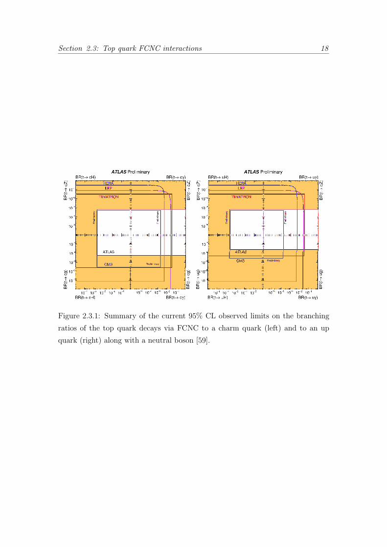
Figure 2.3.1 shows a summary of the current 95% CL observed limits on the
branching rations specifically of the top decays via FCNC to a charm quark with
a neutral boson and to an up quark with a neutral boson.
Section 2.3: Top quark FCNC interactions 18
Figure 2.3.1: Summary of the current 95% CL observed limits on the branching
ratios of the top quark decays via FCNC to a charm quark (left) and to an up
quark (right) along with a neutral boson [59].

Chapter 3
Experimental Setup
Located at the European Organization for Nuclear Research (CERN), the Large
Hadron Collider (LHC) [60] is the world’s highest energy particle accelerator. The
ATLAS experiment [61] is one of the four large experiments that benefit from
the collisions of the particles in the LHC. In this chapter an introduction to the
CERN’s accelerator complex, the LHC and the ATLAS detector is presented.
3.1 CERN
Based on the Franco-Swiss border near Geneva, the CERN was founded in Septem-
ber 29th of 1954 with 12 member states and the acronym CERN Conseil Europeen
pour la Recherche Nucleaire was born. The initial goal of this council was the
study of atomic nuclei and the congregation of scientists. It was soon improved to
the research in the high energy physics focusing in the interactions of subatomic
particles.
CERN has built several accelerators and detectors with distinct targets in the
particle physics field to probe the fundamental structure of the Universe. Figure
3.1.1 shows the accelerators and the detectors currently working at CERN.
Since its beginning, CERN played a major role in the great achievements in particle
physics. Among them are the discovery of neutral currents with the Gargamelle
bubble chamber (1973) [63], the discovery of W± and Z boson with the UA1
19

Section 3.2: The Large Hadron Collider 20
Figure 3.1.1: Schematic view of the CERN accelerator complex.[62]
and UA2 experiments (1983) [64, 65], the determination of the number of light
neutrino families at the Large Electron-Positron Collider (LEP) (1989) [66], the
discovery of direct CP violation [67](1999) and the latest discovery of the Higgs
boson [68, 69](2012) with a mass of 125 GeV observed by the ATLAS and the
CMS collaboration to fulfill the SM.
Through the years, the CERN laboratory has become more than an european
organization having already 22 member states and receiving more than 12,000
scientists from over 70 countries for their research.
3.2 The Large Hadron Collider
The latest addition to the CERN’s accelerator complex was the Large Hadron
Collider [60]. Today it is the world’s largest and most powerful particle accelerator.
21 Section 3.3: The Large Hadron Collider
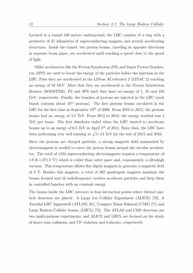
Located in a tunnel 100 meters underground, the LHC consists of a ring with a
perimeter of 27 kilometers of superconducting magnets and several accelerating
structures. Inside the tunnel, two proton beams, traveling in opposite directions
in separate beam pipes, are accelerated until reaching a speed close to the speed
of light.
Older accelerators like the Proton Synchroton (PS) and Super Proton Synchro-
ton (SPS) are used to boost the energy of the particles before the injection in the
LHC. First they are accelerated at the LINear ACcelerator 2 (LINAC 2) reaching
an energy of 50 MeV. After that they are accelerated in the Proton Synchroton
Booster (BOOSTER), PS and SPS until they have an energy of 1, 25 and 450
GeV, respectively. Finally, the bunches of protons are injected in the LHC (each
bunch contains about 1011 protons). The first protons beams circulated in the
LHC for the first time in September 10th of 2008. From 2010 to 2012, the protons
beams had an energy of 3.5 TeV. From 2012 to 2013, the energy reached was 4
TeV per beam. The first shutdown ended when the LHC started to accelerate
beams up to an energy of 6.5 TeV in April 5th of 2015. Since then, the LHC have
been performing very well running at√s=13 TeV for the rest of 2015 and 2016.
Since the protons are charged particles, a strong magnetic field maintained by
electromagnets is needed to curve the proton beams around the circular accelera-
tor. The total of 1232 superconducting electromagnets requires a temperature of
1.9 K (-271.3 °C) which is colder than outer space and, consequently, a ultrahigh
vacuum. This temperature allows this dipole magnets to generate a magnetic field
of 8 T. Besides this magnets, a total of 392 quadrupole magnets maintain the
beams focused and 16 radiofrequency cavities accelerate particles and keep them
in controlled bunches with an constant energy.
The beams inside the LHC intersect in four interaction points where distinct par-
ticle detectors are placed: A Large Ion Collider Experiment (ALICE) [70], A
Toroidal LHC ApparatuS (ATLAS) [61], Compact Muon Solenoid (CMS) [71] and
Large Hadron Collider beauty (LHCb) [72]. The ATLAS and CMS detectors are
two multi-purpose experiments, and ALICE and LHCb are focused on the study
of heavy-ions collisions, and CP violation and b-physics, respectively.
Section 3.3: The ATLAS detector 22
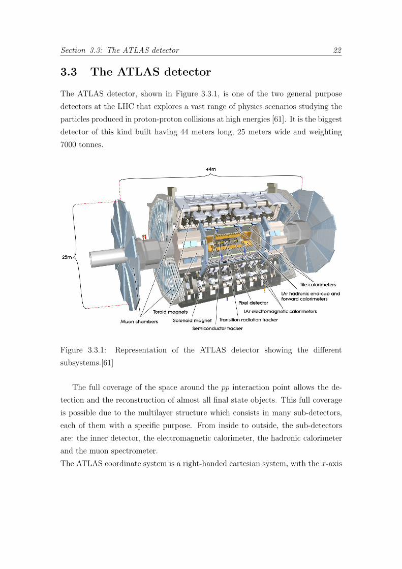
3.3 The ATLAS detector
The ATLAS detector, shown in Figure 3.3.1, is one of the two general purpose
detectors at the LHC that explores a vast range of physics scenarios studying the
particles produced in proton-proton collisions at high energies [61]. It is the biggest
detector of this kind built having 44 meters long, 25 meters wide and weighting
7000 tonnes.
Figure 3.3.1: Representation of the ATLAS detector showing the different
subsystems.[61]
The full coverage of the space around the pp interaction point allows the de-
tection and the reconstruction of almost all final state objects. This full coverage
is possible due to the multilayer structure which consists in many sub-detectors,
each of them with a specific purpose. From inside to outside, the sub-detectors
are: the inner detector, the electromagnetic calorimeter, the hadronic calorimeter
and the muon spectrometer.
The ATLAS coordinate system is a right-handed cartesian system, with the x-axis

23 Section 3.3: The ATLAS detector
towards the center of the LHC ring, the y-axis pointing upwards and the z-axis
pointing along the beam pipe. The nominal interaction point is defined as the
origin of the coordinate system. To better describe rotational invariant properties,
the spherical coordinates (R, φ, θ) are used and defined by
R =√
x2 + y2, φ = arctan(y/x), θ = arctan(R/z). (3.3.1)
The azimuthal angle φ is the angle between the x-axis and the y-axis and the
polar angle θ is defined as the angle between the z-axis and the x – y plane.
The azimuthal angle is defined within φ ∈ [−π, π] and the polar angle within θ ∈[0, π]. The particle momentum px, py and pz are defined along the x, y and z-axis,
respectively. However, it is widely used the transverse momentum pT defined by
pT =√
px2 + py2. (3.3.2)
The pseudorapidity is another important variable used in the ATLAS experiment
and it is defined by
η ≡ 1
2ln(
|−→P |+ pZ
|−→P | − pZ). (3.3.3)
Since the difference in the pseudorapidity of two particles ∆y is independent of
Lorentz boosts along the beam axis and, for massless particles, the pseudorapid-
ity coincides with the rapidity y, the pseudorapidity provides a physically better
variable. It can be also written in terms of the polar angle as
η ≡ − ln(tanθ
2). (3.3.4)
Another variable used is the distance between two particles ∆R defined in terms
of the difference in the pseudorapidity and the difference in the azimuthal angle
between the two particles:
∆R ≡√
∆η2 +∆φ2. (3.3.5)
3.3.1 Inner detector
The inner detector, shown in Figure 3.3.2, is a very compact and highly sensitive
part of ATLAS and the closest system to the beam pipe allowing the study of
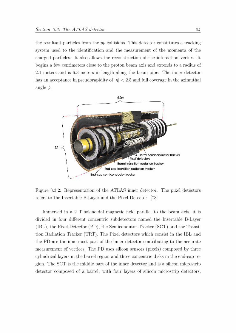
Section 3.3: The ATLAS detector 24
the resultant particles from the pp collisions. This detector constitutes a tracking
system used to the identification and the measurement of the momenta of the
charged particles. It also allows the reconstruction of the interaction vertex. It
begins a few centimeters close to the proton beam axis and extends to a radius of
2.1 meters and is 6.3 meters in length along the beam pipe. The inner detector
has an acceptance in pseudorapidity of |η| < 2.5 and full coverage in the azimuthal
angle φ.
Figure 3.3.2: Representation of the ATLAS inner detector. The pixel detectors
refers to the Insertable B-Layer and the Pixel Detector. [73]
Immersed in a 2 T solenoidal magnetic field parallel to the beam axis, it is
divided in four different concentric subdetectors named the Insertable B-Layer
(IBL), the Pixel Detector (PD), the Semicondutor Tracker (SCT) and the Transi-
tion Radiation Tracker (TRT). The Pixel detectors which consist in the IBL and
the PD are the innermost part of the inner detector contributing to the accurate
measurement of vertices. The PD uses silicon sensors (pixels) composed by three
cylindrical layers in the barrel region and three concentric disks in the end-cap re-
gion. The SCT is the middle part of the inner detector and is a silicon microstrip
detector composed of a barrel, with four layers of silicon microstrip detectors,
25 Section 3.3: The ATLAS detector
and two end-caps, each with nine disks. The TRT is the outermost part the in-
ner detector and consists of 4 mm diameter gaseous straw tubes interleaved with
transition radiation material.
Combining the information from the four subdetectors, the transverse momentum
resolution measured in the plane perpendicular to the beam axis is [61]
σpTpT
=0.05%
GeVpT ⊕ 1%. (3.3.6)
3.3.2 Calorimeters
The ATLAS calorimeter system, shown in Figure 3.3.3, is used to provide an
accurate measurement of particles energies by absorbing them and measuring the
shower properties, which eases the particle identification. The calorimeters are
designed to stop the majority of the particles, except for muons and neutrinos.
Each of the calorimeters are divided into a central barrel part and two symmetric
end-caps.
The calorimeter system stops most of the particles from arriving to the muon
spectrometer preventing them from being identified as muons. Given the neutrinos
do not leave any signatures to be observed and do not interact with the detector
material, the called missing transverse energy EmissT could be obtained since the
four-momentum carried by neutrino implies as unbalance in the total momentum
available in the event. The good measurement of EmissT is an important mission
in the ATLAS calorimeters since this variable is a crucial discriminant for many
physics searches.
The electromagnetic calorimeter force the decay and then measure the energy of the
electromagnetic particles which are leptons or photons. The hadronic calorimeter
measures the energy deposition from the hadronic showers of high energy hadrons
which are protons or neutrons. The components of the calorimetry system are:
the Liquid Argon (LAr) electromagnetic calorimeter, the LAr hadronic end-cap
calorimeter (HEC), the LAr forward calorimeter (FCal) and the Tile calorimeter
(TileCal). The electromagnetic and the hadronic calorimeters cover a region of |η|< 3.2 and |η| < 4.9, respectively.

Section 3.3: The ATLAS detector 26
The LAr electromagnetic calorimeter uses liquid argon as active material and lead
Figure 3.3.3: Open view of the ATLAS calorimeter system.[74]
plates as absorber composing a sampling detector of one barrel and two end-caps.
The target energy resolution for the electromagnetic calorimeter is [61]
σEE
=10%√E
⊕ 17%
E⊕ 0.7%, (3.3.7)
with E measured in GeV.
The TileCal hadronic calorimeter is also a sampling calorimeter using steel
(as absorber material) and scintillating plastic tiles (as active material) placed in
one central barrel and two extended barrels. The target energy resolution for the
TileCal hadronic calorimeter is [61]
σEE
=50%√E
⊕ 3% (3.3.8)
with E measured in GeV.
3.3.3 Muon spectrometer
The muon spectrometer, shown in Figure 3.3.4, is a combination of toroidal super-
conducting magnets and precision chambers designed to detect and measure the

27 Section 3.3: The ATLAS detector
momentum of the muons. As muons minimally interact with the other parts of the
detector and have long lifetimes, they are identified and measured in the outermost
detector layer. This system is by far the largest tracking system in ATLAS since
it extends from a radius of 4.25 m around the calorimeters out to the full radius
of the detector (which is 11 m). This detector system covers a region of |η| < 2.7.
It is also designed to trigger the muons in the region |η| < 2.4.
Figure 3.3.4: Representation of the ATLAS muon spectrometer.[75]
It is composed by four distinct chambers: Thin Gap Chambers (TGC), Resis-
tive Plate Chambers (RPC), Monitored Drift Tubes (MDT) and Cathode Strip
Chambers (CSC). Due to the magnetic field provided by the toroidal magnets,
this subdetectors measure the muons momentum through the measurement of the
curvature of the deflected muon trajectory. The muon spectrometer was designed
to provide a transverse momentum resolution of [61]
σpTpT
= 10% at pT = 1 TeV. (3.3.9)
Section 3.3: The ATLAS detector 28
3.3.4 Magnet system
The ATLAS magnet system allows the measurement of the charged particles mo-
mentum and it is designed to provide a field mostly orthogonal to the particle
trajectory. It is composed of four large superconducting magnets: one central
solenoid magnet, one barrel toroid, and two end-cap toroids.
The central solenoid magnet encloses the inner detector and provides a high mag-
netic field to bend the trajectory of charged particles allowing the momentum
measurement by the tracking system.
The toroidal magnet system is divided in three parts with a barrel part placed
around the central calorimeter and two end-caps placed at each end of the detector.
Each of these toroidal magnets has eight identical coils built radially in a symmetric
way around the beam pipe. The toroidal magnet system provides the magnetic
field for additional bending of the muon trajectories in order to measure with
precision their momentum in the muon barrel and end-cap spectrometers.
In contrast with the central solenoid magnet which produces a uniform magnetic
field of approximately 0.5 T, the magnetic field produced by the toroidal magnets
it varies from 0.15 T to 2.5 T [61].
3.3.5 Trigger and data acquisition system
The production cross-section of inelastic proton-proton scattering events at the
LHC is several orders of magnitude higher than the cross-section of elastic scat-
tering. Consequently, millions of uninteresting collisions happen every second.
Besides that, the high collision rate of 40 million events per second at the LHC
running conditions does not allow the storage and analysis of all amount of data
generated.
To reduce the flow of data to acceptable levels, the ATLAS trigger and data
acquisition system selects in real time events with different characteristics that
make them interesting for physics analyses. The trigger system works in three
stages: the level 1 hardware trigger (L1), the high level software trigger containing
the level 2 (L2) and event filter triggers (EF) [61]. In nominal conditions, the
29 Section 3.3: The ATLAS detector
L1, L2 and EF system reduces the event rate to 75 kHz, 3.5 kHz and 200 Hz,
respectively.
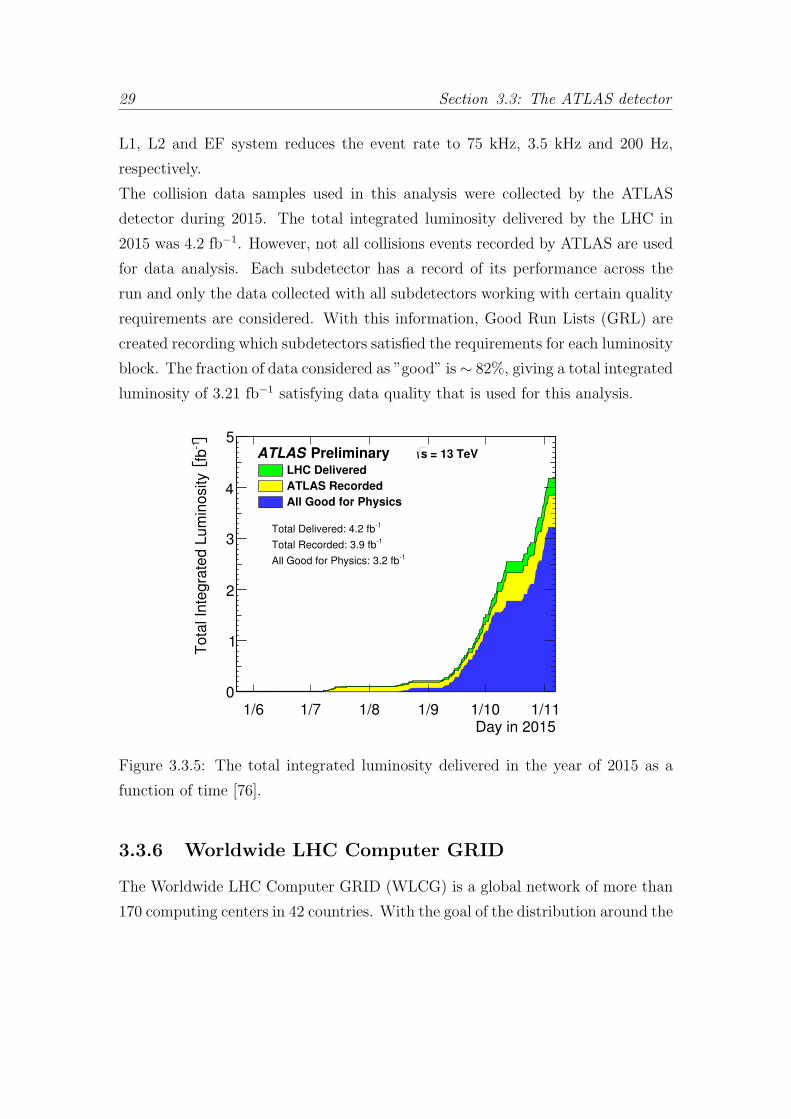
The collision data samples used in this analysis were collected by the ATLAS
detector during 2015. The total integrated luminosity delivered by the LHC in
2015 was 4.2 fb−1. However, not all collisions events recorded by ATLAS are used
for data analysis. Each subdetector has a record of its performance across the
run and only the data collected with all subdetectors working with certain quality
requirements are considered. With this information, Good Run Lists (GRL) are
created recording which subdetectors satisfied the requirements for each luminosity
block. The fraction of data considered as ”good” is∼ 82%, giving a total integrated
luminosity of 3.21 fb−1 satisfying data quality that is used for this analysis.
Day in 2015
-1fb
To
tal In
teg
rate
d L
um
ino
sity
0
1
2
3
4
5
1/6 1/7 1/8 1/9 1/10 1/11
= 13 TeVs PreliminaryATLASLHC Delivered ATLAS Recorded
All Good for Physics
Total Delivered: 4.2 fb-1
Total Recorded: 3.9 fb-1
All Good for Physics: 3.2 fb-1
Figure 3.3.5: The total integrated luminosity delivered in the year of 2015 as a
function of time [76].
3.3.6 Worldwide LHC Computer GRID
The Worldwide LHC Computer GRID (WLCG) is a global network of more than
170 computing centers in 42 countries. With the goal of the distribution around the

Section 3.3: The ATLAS detector 30
globe the data from the LHC experiments, the WLCG is linking up national and
international grid infrastructures. This worldwide network is designed to store,
organize and analyze the ∼ 30 Petabytes of data annually generated at the LHC
[77]. The WLCG is divided in different layers, called tiers, each one with distinct
purposes.
The Tier 0 is the CERN data Centre located in Geneva and also at the Wigner
Research Centre for Physics in Budapest. The two sites are connected by two
dedicated 100 Gigabit/s data links. The Tier 0 is responsible for the safe-keeping
of raw data, first pass reconstruction, distribution of raw data and reconstruction
output to the Tier 1.
The Tier 1 is composed by thirteen large computer centres. They are responsible
for the safe-keeping of a proportional share of raw and reconstructed data, large-
scale reprocessing and safe-keeping of corresponding output, distribution of data
to Tier 2 and safe-keeping of a share of simulated data produced at these Tier 2.
The Tier 2 is composed by around 160 sites typically located at universities and
other scientific institutes. This sites can store data and provide computing power
for specific analysis tasks. The individual scientists can access and process the
data through the Tier 3 computing resources consisting of local clusters.

31 Section 3.3: The ATLAS detector
Figure 3.3.6: Representation of the structure of the tiers 0, 1 and 2. The various
locations of the thirteen computer centres of tier 1 can also be found [78].

Section 3.3: The ATLAS detector 32

Chapter 4
Event analysis
This chapter presents the search analysis focused on the top FCNC process where
a top quark and a neutral Z boson is produced. A trileptonic topology with
three leptons, two charged leptons coming from the decay of the Z boson and
one charged lepton along with one neutrino coming and one b-tagged jet from the
decay of the top quark is considered. This topology was chosen since the final state
consists in a clear signature of three leptons and just one jet [79]. The consequent
loss in acceptance are compensated with the gain in efficiency. An overview of
the analysis is presented taking in account the objects definition, data and Monte
Carlo (MC) simulation samples, analysis strategy and systematic uncertainties.
The analysis presented in this thesis uses the A++ code as analysis code which
was developed by the Humboldt University group in Berlin [80].
4.1 Data sample and triggers
The data sample analyzed in this search was collected with the ATLAS detector
in proton-proton collisions at a centre-of-mass energy of 13 TeV between July and
November of 2015. A total integrated luminosity of 3.21 fb−1 was recorded after
requiring all subdetectors to be fully operational during the data taking.
The analyzed events are selected using single electron and muon triggers with
different pT thresholds and then are combined in a logical OR in order to increase
33

Section 4.2: Objects definition 34
the overall efficiency [81]. The single electron triggers used are HLT_e60_lhmedium
and HLT_e120_lhloose. Beside these, HLT_e24_lhmedium_L1EM20VH for data and
HLT_e24_lhmedium_L1EM18VH for MC triggers are used where the only difference is
due to the transverse energy threshold of the electromagnetic cluster. The single
muon triggers used are HLT_mu20_iloose_L1MU15 and HLT_mu50 [82]. The pT
thresholds are 24 or 60 GeV for the electron triggers and 20 or 50 GeV for the
muon triggers. In order to share information, a process named triggers match is
performed where a geometrical acceptance is applied to the triggers information
with a chosen ∆R. Due to the precise momentum measurement and the low
misidentification rate, muons are the objects best able to be measured and provide
an excellent trigger matching.
4.2 Objects definition
The physics objects studied in this analysis are electrons, muons and hadronic jets
including b-tagged jets.
Electron candidates [83] are reconstructed from energy deposits in the electromag-
netic calorimeter that are matched with tracks in the inner detector. Only electron
candidates with pT > 25 GeV in the central region defined by the range |ηcluster| <2.47 (|ηcluster| corresponds to the pseudorapidity of the cluster associated with the
electron candidate) are selected. There are three electron identification selections:
Medium, Loose and Tight to the specific needs of different physics analyses. In
this analysis, electrons candidates must satisfy tight quality criteria.
Muon candidates [84] are reconstructed from tracks in the layers of the muon spec-
trometer which matched with the corresponding tracks in the inner detector. Only
muon candidates with pT > 25 GeV and |η| < 2.5 are selected. A longitudinal
impact parameter with respect to the interaction point smaller than 2 mm is re-
quired to ensure that the muon candidate is a muon produced in the collisions and
not cosmic muons. Concerning the muon reconstruction, there are four identifi-
cation selections: Medium, Loose, Tight and High-pT. Loose, Medium and Tight
are inclusive categories where muons identified with tighter requirements are also
35 Section 4.2: Objects definition
included in the looser categories. In this analysis, muon candidates must satisfy
tight quality criteria.
Jets are reconstructed using the anti-kt algorithm [85, 86, 87] with a radius param-
eter of ∆R=0.4 using calibrated topological clusters built from energy deposits in
the hadronic calorimeter. The calibration of topological clusters [88, 89] is made to
correct the cluster energy for the effects of non-compensation, dead material and
out-of-cluster leakage. The corrections are obtained through simulation of neutral
and charged particles. During the jets reconstruction electrons and hadronic en-
ergy deposition can not be distinguish. To remove this overlap between electrons
and jets, any jet identified within a cone of radius ∆R < 0.2 is excluded. After
that, any remaining electrons or muons within a radius of ∆R < 0.4 of a select
jet are excluded. After energy calibration [90], only jets that satisfy pT > 30 GeV
and |η| < 2.5 are selected.
The identification of jets coming from the bottom quark, known as b-tagged jets,
is made using the MV2c20 algorithm. The MV2c20 algorithm uses a boosted de-
cision tree algorithm to discriminate b-jets from light (u,d,s-quark or gluon jets)
where the training is performed on a set of around 5 million tt events. With a
total of 24 input variables, this b-tagging algorithm takes into account parameters
like transverse momentum, pseudorapidity, invariant mass of tracks and distances
between others. Through a cut on the MV2 output distribution, the b-tagging
algorithm is characterized by different operating points. The operating points are
calibrated in a sample of simulated tt events and provide a specific b-tagging effi-
ciency of 60%, 70%, 77% or 85% [91].The performance of the b-tagging algorithm
is affected by the capability to correctly identify jets coming from a real b-quark
compared to the probability of mistakenly b-tagging a jet originating from a c-
quark or a light-flavour parton (u,d,s-quark or gluon). The b-tagging efficiencies
with the c-jet and light-jets rejection rates are presented in Table 4.2.1.

Section 4.3: Objects definition 36
b-jet efficiency c-jet rejection Light-jet rejection
60% 21 1900
70% 8.1 440
77% 4.5 140
85% 2.6 28
Table 4.2.1: Operating points for the MV2c20 b-tagging algorithm including the
c-jet and light-jets rejection rates [91].
For the analysis presented in this thesis, the operating point used is the one with
a jet efficiency of 77% due to the reasonable balance between the efficiency of the
identification of b-jets and the rejection of light quarks. The tagging efficiency to
b, c and light-flavour jets for the MV2c20 algorithm with the 77% operating point
as a function of jet pT and |η| are presented in Figure 4.2.1.
(a) (b)
Figure 4.2.1: The efficiency to tag b (green), c (blue) and light-flavour (red) jets
for the MV2c20 tagger with the 77% working point. Efficiencies are shown as a
function of the jet (a) pT and (b) |η| [92, 93].

37 Section 4.3: Analysis strategy
4.3 Analysis strategy
The strategy of this analysis consists in a set of requirements taking into account
the final state of tZ production via FCNC. The tZ production via FCNC consists
in the production of a Z boson which decays to two leptons, the production of
a top quark which decays to a W boson and a bottom quark. The final state is
characterized by two leptons coming from the Z boson, one charged lepton and
one neutral lepton (neutrino) coming from the W boson decay and one b-tagged
jet coming from the hadronisation of a bottom quark.
At the first selection level is required that events contain, exactly, one jet and
three leptons. In the next selection level, the events without a Z boson candidate
are excluded. The two leptons with higher pT are used to reconstruct the Z boson
candidate. The Z boson candidates are reconstructed with a pair of Opposite-Sign
Same-Flavour (OSSF) leptons (electrons or muons) with a invariant mass higher
than 70 Gev and lower than 110 GeV (which are around 20 GeV of difference
from the measured Z boson mass 91.19 GeV [5]). In the case of two Z bosons
reconstructed, the candidate with the mass closest to 91.19 GeV is selected. The
lepton not chosen as coming from the decay of the Z boson is used to reconstruct
the decay of the W boson. It is assumed that the W boson decays leptonically,
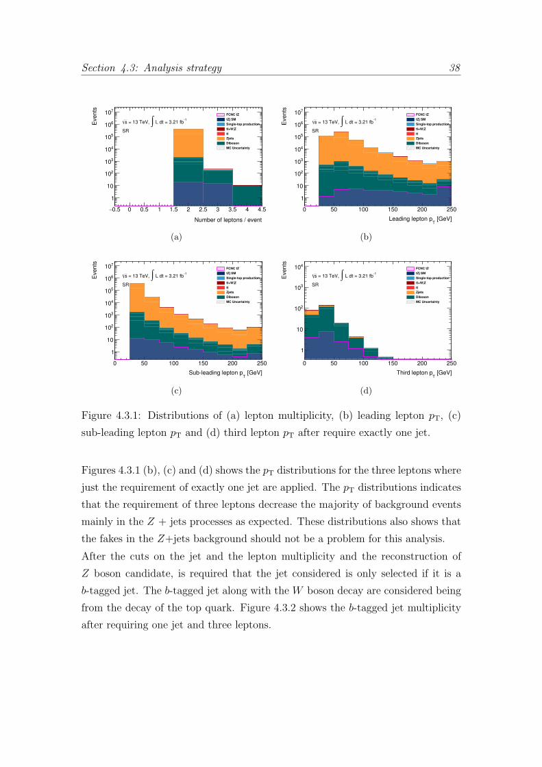
having a charged and a neutral lepton as final state. Figure 4.3.1 shows the lepton
multiplicity and the three leptons pT distributions after requiring events with ex-
actly one jet. The filled region corresponds to the multiple background processes
predictions and the solid line is the signal hypothesis for the tZ production through
FCNC processes.
Figure 4.3.1 (a) shows the lepton multiplicity. The signal sample has more events
in the regions with two and three leptons, which corresponds to the W boson
decaying hadronically and leptonically, respectively. In the dileptonic region the
background is defined by the Z+jets and dibosons processes. However, in the
trileptonic region the background corresponds mainly to the diboson processes. In
this analysis, it is studied the process where the W boson decays leptonically.
Section 4.3: Analysis strategy 38
Number of leptons / event
0.5− 0 0.5 1 1.5 2 2.5 3 3.5 4 4.5
Events
1
10
210
310
410
510
610
710 FCNC tZ
tZj SM
Single-top production
+W|Ztt
tt
Zjets
Diboson
MC Uncertainty
-1 L dt = 3.21 fb∫ = 13 TeV, s
SR
(a)
[GeV]T
Leading lepton p
0 50 100 150 200 250
Events
1
10
210
310
410
510
610
710 FCNC tZ
tZj SM
Single-top production
+W|Ztt
tt
Zjets
Diboson
MC Uncertainty
-1 L dt = 3.21 fb∫ = 13 TeV, s
SR
(b)
[GeV]T
Sub-leading lepton p
0 50 100 150 200 250
Events
1
10
210
310
410
510
610
710 FCNC tZ
tZj SM
Single-top production
+W|Ztt
tt
Zjets
Diboson
MC Uncertainty
-1 L dt = 3.21 fb∫ = 13 TeV, s
SR
(c)
[GeV]T
Third lepton p
0 50 100 150 200 250
Events
1
10
210
310
410 FCNC tZ
tZj SM
Single-top production
+W|Ztt
tt
Zjets
Diboson
MC Uncertainty
-1 L dt = 3.21 fb∫ = 13 TeV, s
SR
(d)
Figure 4.3.1: Distributions of (a) lepton multiplicity, (b) leading lepton pT, (c)
sub-leading lepton pT and (d) third lepton pT after require exactly one jet.
Figures 4.3.1 (b), (c) and (d) shows the pT distributions for the three leptons where
just the requirement of exactly one jet are applied. The pT distributions indicates
that the requirement of three leptons decrease the majority of background events
mainly in the Z + jets processes as expected. These distributions also shows that
the fakes in the Z+jets background should not be a problem for this analysis.
After the cuts on the jet and the lepton multiplicity and the reconstruction of
Z boson candidate, is required that the jet considered is only selected if it is a
b-tagged jet. The b-tagged jet along with the W boson decay are considered being
from the decay of the top quark. Figure 4.3.2 shows the b-tagged jet multiplicity
after requiring one jet and three leptons.
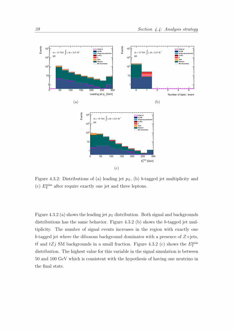
39 Section 4.4: Analysis strategy
[GeV]T
Leading jet p
0 50 100 150 200 250 300
Events
1
10
210
310
410 FCNC tZ
tZj SM
Single-top production
+W|Ztt
tt
Zjets
Diboson
MC Uncertainty
-1 L dt = 3.21 fb∫ = 13 TeV, s
SR
(a)
Number of bjets / event
0 1 2 3 4 5
Events
1
10
210
310
410 FCNC tZ
tZj SM
Single-top production
+W|Ztt
tt
Zjets
Diboson
MC Uncertainty
-1 L dt = 3.21 fb∫ = 13 TeV, s
SR
(b)
[GeV]miss
TE
0 50 100 150 200 250 300
Events
1
10
210
310
410 FCNC tZ
tZj SM
Single-top production
+W|Ztt
tt
Zjets
Diboson
MC Uncertainty
-1 L dt = 3.21 fb∫ = 13 TeV, s
SR
(c)
Figure 4.3.2: Distributions of (a) leading jet pT, (b) b-tagged jet multiplicity and
(c) EmissT after require exactly one jet and three leptons.
Figure 4.3.2 (a) shows the leading jet pT distribution. Both signal and backgrounds
distributions has the same behavior. Figure 4.3.2 (b) shows the b-tagged jet mul-
tiplicity. The number of signal events increases in the region with exactly one
b-tagged jet where the dibosons background dominates with a presence of Z+jets,
tt and tZj SM backgrounds in a small fraction. Figure 4.3.2 (c) shows the EmissT
distribution. The highest value for this variable in the signal simulation is between
50 and 100 GeV which is consistent with the hypothesis of having one neutrino in
the final state.
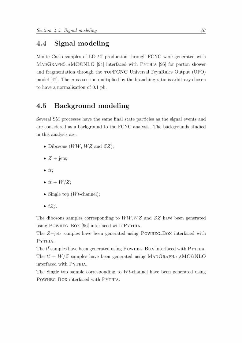
Section 4.5: Signal modeling 40
4.4 Signal modeling
Monte Carlo samples of LO tZ production through FCNC were generated with
MadGraph5 aMC@NLO [94] interfaced with Pythia [95] for parton shower
and fragmentation through the topFCNC Universal FeynRules Output (UFO)
model [47]. The cross-section multiplied by the branching ratio is arbitrary chosen
to have a normalisation of 0.1 pb.
4.5 Background modeling
Several SM processes have the same final state particles as the signal events and
are considered as a background to the FCNC analysis. The backgrounds studied
in this analysis are:
• Dibosons (WW , WZ and ZZ);
• Z + jets;
• tt;
• tt + W/Z;
• Single top (Wt-channel);
• tZj.
The dibosons samples corresponding to WW ,WZ and ZZ have been generated
using Powheg Box [96] interfaced with Pythia.
The Z+jets samples have been generated using Powheg Box interfaced with
Pythia.
The tt samples have been generated using Powheg Box interfaced with Pythia.
The tt + W/Z samples have been generated using MadGraph5 aMC@NLO
interfaced with Pythia.
The Single top sample corresponding to Wt-channel have been generated using
Powheg Box interfaced with Pythia.

41 Section 4.5: Background modeling
The tZj sample have been generated using MadGraph5 aMC@NLO interfaced
with Pythia.
The background processes described are simulated in multiple MC samples which
cross-sections and generators used are shown in Table 4.5.1.
Process σ (pb) Generator
WW → lνlν 10.631 Powheg Box + Pythia
WZ → lνll 4.462 Powheg Box + Pythia
WZ → qqll 3.285 Powheg Box + Pythia
ZZ → llll 1.257 Powheg Box + Pythia
ZZ → lνlν 0.925 Powheg Box + Pythia
ZZ → qqll 2.274 Powheg Box + Pythia
Z → ee 1950.63 Powheg Box + Pythia
Z → µµ 1950.63 Powheg Box + Pythia
Z → ττ 1950.63 Powheg Box + Pythia
tt 451.664 Powheg Box + Pythia
tt + W 0.221 MadGraph5 aMC@NLO + Pythia
tt + W 0.176 MadGraph5 aMC@NLO + Pythia
tt + W 0.171 MadGraph5 aMC@NLO + Pythia
tt + Z 0.013 MadGraph5 aMC@NLO + Pythia
tt + Z 0.023 MadGraph5 aMC@NLO + Pythia
tt + Z 0.013 MadGraph5 aMC@NLO + Pythia
tt + Z 0.023 MadGraph5 aMC@NLO + Pythia
tt + Z 0.013 MadGraph5 aMC@NLO + Pythia
tt + Z 0.024 MadGraph5 aMC@NLO + Pythia
Wt Channel 35.845 Powheg Box + Pythia
tZj 0.240 MadGraph aMC@NLO + Pythia
Table 4.5.1: Background MC samples with the corresponding cross-sections and
generators used in the analysis presented in this thesis.
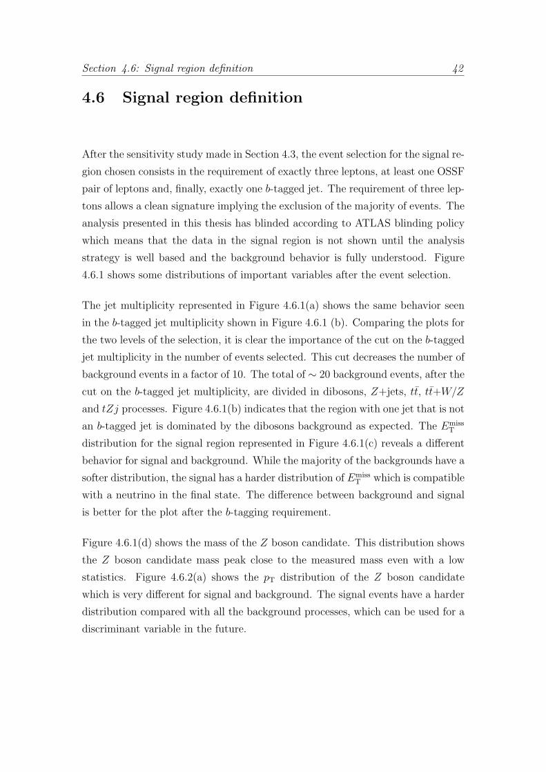
Section 4.6: Signal region definition 42
4.6 Signal region definition
After the sensitivity study made in Section 4.3, the event selection for the signal re-
gion chosen consists in the requirement of exactly three leptons, at least one OSSF
pair of leptons and, finally, exactly one b-tagged jet. The requirement of three lep-
tons allows a clean signature implying the exclusion of the majority of events. The
analysis presented in this thesis has blinded according to ATLAS blinding policy
which means that the data in the signal region is not shown until the analysis
strategy is well based and the background behavior is fully understood. Figure
4.6.1 shows some distributions of important variables after the event selection.
The jet multiplicity represented in Figure 4.6.1(a) shows the same behavior seen
in the b-tagged jet multiplicity shown in Figure 4.6.1 (b). Comparing the plots for
the two levels of the selection, it is clear the importance of the cut on the b-tagged
jet multiplicity in the number of events selected. This cut decreases the number of
background events in a factor of 10. The total of ∼ 20 background events, after the
cut on the b-tagged jet multiplicity, are divided in dibosons, Z+jets, tt, tt+W/Z
and tZj processes. Figure 4.6.1(b) indicates that the region with one jet that is not
an b-tagged jet is dominated by the dibosons background as expected. The EmissT
distribution for the signal region represented in Figure 4.6.1(c) reveals a different
behavior for signal and background. While the majority of the backgrounds have a
softer distribution, the signal has a harder distribution of EmissT which is compatible
with a neutrino in the final state. The difference between background and signal
is better for the plot after the b-tagging requirement.
Figure 4.6.1(d) shows the mass of the Z boson candidate. This distribution shows
the Z boson candidate mass peak close to the measured mass even with a low
statistics. Figure 4.6.2(a) shows the pT distribution of the Z boson candidate
which is very different for signal and background. The signal events have a harder
distribution compared with all the background processes, which can be used for a
discriminant variable in the future.

43 Section 4.6: Signal region definition
Number of jets / event
0 1 2 3 4 5
Events
0
100
200
FCNC tZ
tZj SM
Single-top production
+W|Ztt
tt
Zjets
Diboson
MC Uncertainty
-1 L dt = 3.21 fb∫ = 13 TeV, s
SR
Number of jets / event
0 1 2 3 4 5
Events
0
5
10
15
20
FCNC tZ
tZj SM
Single-top production
+W|Ztt
tt
Zjets
Diboson
MC Uncertainty
-1 L dt = 3.21 fb∫ = 13 TeV, s
SR
(a)
Number of bjets / event
0 1 2 3 4 5
Events
0
50
100
150
200
FCNC tZ
tZj SM
Single-top production
+W|Ztt
tt
Zjets
Diboson
MC Uncertainty
-1 L dt = 3.21 fb∫ = 13 TeV, s
SR
Number of bjets / event
0 1 2 3 4 5
Events
0
5
10
15
20
FCNC tZ
tZj SM
Single-top production
+W|Ztt
tt
Zjets
Diboson
MC Uncertainty
-1 L dt = 3.21 fb∫ = 13 TeV, s
SR
(b)
[GeV]miss
TE
0 50 100 150 200 250 300
Events
0
20
40
60
80
FCNC tZ
tZj SM
Single-top production
+W|Ztt
tt
Zjets
Diboson
MC Uncertainty
-1 L dt = 3.21 fb∫ = 13 TeV, s
SR
[GeV]miss
TE
0 50 100 150 200 250 300
Events
0
5
10 FCNC tZ
tZj SM
Single-top production
+W|Ztt
tt
Zjets
Diboson
MC Uncertainty
-1 L dt = 3.21 fb∫ = 13 TeV, s
SR
(c)
M(lep,lep) [GeV]
60 70 80 90 100 110 120
Events
0
50
100
FCNC tZ
tZj SM
Single-top production
+W|Ztt
tt
Zjets
Diboson
MC Uncertainty
-1 L dt = 3.21 fb∫ = 13 TeV, s
SR
M(lep,lep) [GeV]
60 70 80 90 100 110 120
Events
0
5
10
FCNC tZ
tZj SM
Single-top production
+W|Ztt
tt
Zjets
Diboson
MC Uncertainty
-1 L dt = 3.21 fb∫ = 13 TeV, s
SR
(d)
Figure 4.6.1: Signal region distributions of (a) jet multiplicity, (b) b-tagged jet
multiplicity, (c) EmissT and (d) Z boson candidate mass before (left) and after
(right) the b-tagged jet requirement.
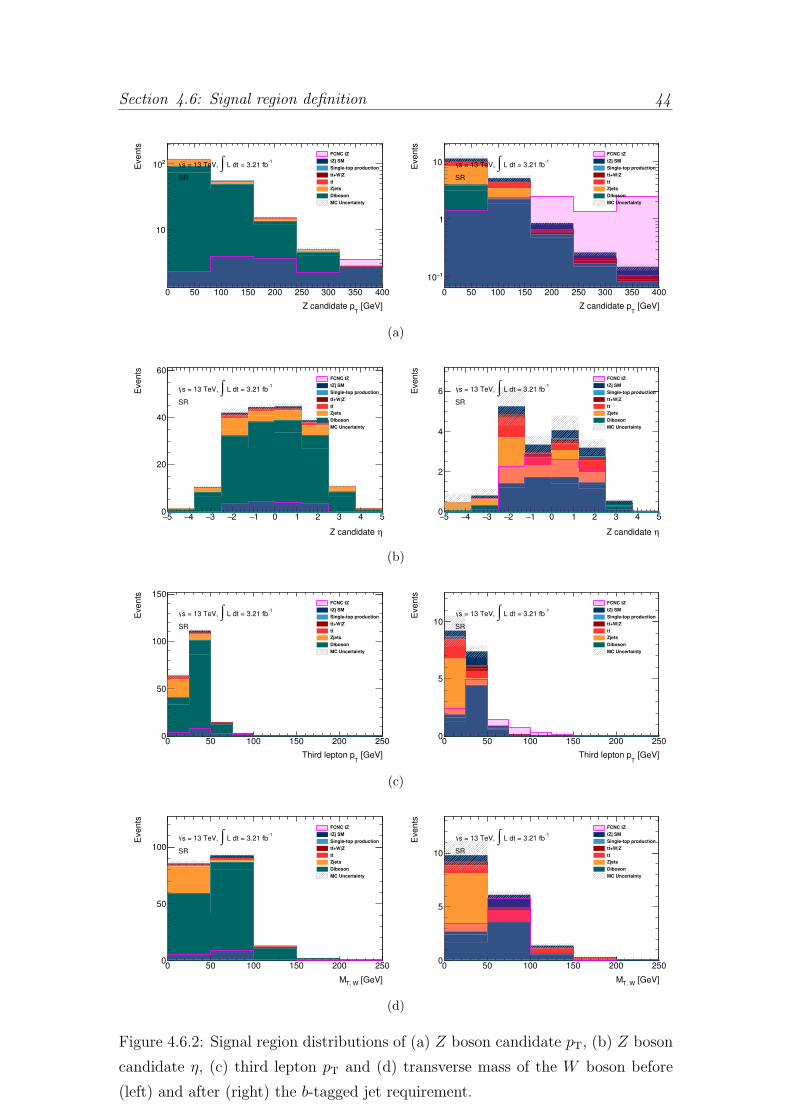
Section 4.6: Signal region definition 44
[GeV]T
Z candidate p
0 50 100 150 200 250 300 350 400
Events
10
210
FCNC tZ
tZj SM
Single-top production
+W|Ztt
tt
Zjets
Diboson
MC Uncertainty
-1 L dt = 3.21 fb∫ = 13 TeV, s
SR
[GeV]T
Z candidate p
0 50 100 150 200 250 300 350 400
Events
1−10
1
10FCNC tZ
tZj SM
Single-top production
+W|Ztt
tt
Zjets
Diboson
MC Uncertainty
-1 L dt = 3.21 fb∫ = 13 TeV, s
SR
(a)
ηZ candidate
5− 4− 3− 2− 1− 0 1 2 3 4 5
Events
0
20
40
60FCNC tZ
tZj SM
Single-top production
+W|Ztt
tt
Zjets
Diboson
MC Uncertainty
-1 L dt = 3.21 fb∫ = 13 TeV, s
SR
ηZ candidate
5− 4− 3− 2− 1− 0 1 2 3 4 5
Events
0
2
4
6
FCNC tZ
tZj SM
Single-top production
+W|Ztt
tt
Zjets
Diboson
MC Uncertainty
-1 L dt = 3.21 fb∫ = 13 TeV, s
SR
(b)
[GeV]T
Third lepton p
0 50 100 150 200 250
Events
0
50
100
150FCNC tZ
tZj SM
Single-top production
+W|Ztt
tt
Zjets
Diboson
MC Uncertainty
-1 L dt = 3.21 fb∫ = 13 TeV, s
SR
[GeV]T
Third lepton p
0 50 100 150 200 250
Events
0
5
10
FCNC tZ
tZj SM
Single-top production
+W|Ztt
tt
Zjets
Diboson
MC Uncertainty
-1 L dt = 3.21 fb∫ = 13 TeV, s
SR
(c)
[GeV]T, WM
0 50 100 150 200 250
Events
0
50
100
FCNC tZ
tZj SM
Single-top production
+W|Ztt
tt
Zjets
Diboson
MC Uncertainty
-1 L dt = 3.21 fb∫ = 13 TeV, s
SR
[GeV]T, WM
0 50 100 150 200 250
Events
0
5
10
FCNC tZ
tZj SM
Single-top production
+W|Ztt
tt
Zjets
Diboson
MC Uncertainty
-1 L dt = 3.21 fb∫ = 13 TeV, s
SR
(d)
Figure 4.6.2: Signal region distributions of (a) Z boson candidate pT, (b) Z boson
candidate η, (c) third lepton pT and (d) transverse mass of the W boson before
(left) and after (right) the b-tagged jet requirement.

45 Section 4.7: Signal region definition
The Z boson candidate η represented in Figure 4.6.2(b) shows the majority
of events located in the region where η is zero. The third lepton pT distribution
shown in Figure 4.6.2(c) is characterized by a harder distribution for the signal
events when compared with the background processes. This distribution shows
the behavior of a possible distribution variable. In Figure 4.6.2(d), the transverse
mass of theW boson is shown. This observable is computed considering the lepton
associated with the W boson and the missing transverse energy (EmissT ):
MT(W ) =√
(ElT + Emiss
T )2 − (plx + pmissx )2 − (ply + pmiss
y )2 (4.6.1)
Both distributions of this observable, before and after the b-tagging requirement,
shows the signal events located in the region between 50 and 100 GeV. This be-
havior is consistent with one neutrino in the final state which is the case for the
signal of this analysis. Along with the Z boson candidate pT, this observable can
be a variable used to discriminate signal and background events.
The events yields to the signal region after the selection are shown in Table 4.6.1.
The number of events in the total background are the sum of the number of events
for all background processes.
Process Signal
FCNC tZ 10.10± 0.37
SM tZj 1.94± 0.04
Single Top 0.08± 0.05
tt + W /Z 0.77± 0.01
tt 2.36± 0.45
Z + jets 5.47± 1.35
Dibosons 7.00± 0.21
Total background 17.63± 1.44
Table 4.6.1: Signal region event yields after the selection criteria. The uncertainties
presented corresponds only to the statistical errors.

Section 4.7: Comparison between data and prediction 46
4.7 Comparison between data and prediction
The selection criteria for the analysis of this thesis was presented in Section 4.3.
This section shows the comparison between the data events with an integrated
luminosity of 3.21 fb−1 recorded with a centre-of-mass energy of√s = 13 TeV at
the ATLAS detector and the MC prediction for the different processes.
4.7.1 Validation regions
Beside the signal region, multiple control regions are defined. While the signal
region is targeted to provide the signal sensitivity, the control regions are defined
to validate the background processes. The following regions are studied:
• Z + jets in a dileptonic topology;
• Z + jets in a trileptonic topology;
• tt in a trileptonic topology;
• Diboson, specifically the WZ process, in a trileptonic topology;
• tZj in a trileptonic topology.
Table 4.7.1 summarizes the event selection of the different control regions.
Z+jets 2L CR Z+jets 3L CR tt CR WZ Diboson CR tZj CR
= 2 leptons = 3 leptons = 3 leptons = 3 leptons = 3 leptons
- - EmissT > 20 GeV - Emiss
T > 20 GeV
- - MT (W ) > 40 GeV - -
≥ 1 OSSF Pair ≥ 1 OSSF Pair ≥ 1 OSSF Pair ≥ 1 OSSF Pair ≥ 1 OSSF Pair
70 GeV < M(ℓℓ) 70 GeV < M(ℓℓ) M(ℓℓ) < 80 GeV 81 GeV < M(ℓℓ) 70 GeV < M(ℓℓ)
M(ℓℓ) < 110 GeV M(ℓℓ) < 110 GeV M(ℓℓ) > 100 GeV M(ℓℓ) < 101 GeV M(ℓℓ) < 110 GeV
≥ 1 Jet ≥ 1 Jet = 2 Jets = 1 Jet ≥ 1 Jet
= 1 b-tagged jet = 1 b-tagged jet = 1 b-tagged jet - = 1 b-tagged jet
Table 4.7.1: Selection criteria used to define the considered control regions.
The selection of the Z+jets control region, taking into account the dileptonic
topology, consists in the requirement of exactly two leptons, at least one OSSF

47 Section 4.7: Comparison between data and prediction
pair of leptons with a reconstructed mass between 70 and 110 GeV and at least
one jet where one is an b-tagged jet.
Figure 4.7.1 shows some distributions to the dileptonic Z+jets control region.
Figure 4.7.1(a) shows the Z boson candidate mass distribution, having a good
agreement between data and MC, with the mass peak in the value of ∼ 91 GeV
(close to the measured Z boson mass). The pT distribution of the Z boson can-
didate, shown in Figure 4.7.1(b), is characterized by low values of this variable
mainly localized in the range of 0 and 150 GeV. In Figure 4.7.1(c), the comparison
between data and MC reveals a good agreement in the η distribution of the Z
boson candidate. The agreement is better before the b-tagging requirement.
The jet multiplicity in Figure 4.7.1(d) shows an excellent agreement in the region
with one jet before and after the b-tagging requirement. In the region with two
jets, the agreement is not so good and gets worse after requiring the b-tagged
jet. Since the normalisation is worse in the region with more than one jet and
the signal region requires exactly one jet, the disagreement between data and MC
will not be significant. The b-tagged jet multiplicity represented in Figure 4.7.2
is characterized by a better data and MC agreement in the region without b-jets
when compared with the region with one b-tagged jet. This behavior is compat-
ible in both distributions (before and after the b-tagging requirement). Knowing
from Figure 4.7.1(d) that the agreement between data and MC is reasonable in
the region with exactly one jet, this not so good agreement in the b-tagged jet
multiplicity should not affect the analysis. Since the Z+jets processes does not
have b-quarks in the final state, it is expected that the majority of the number of
events are excluded after the requirement of one b-tagged jet.
The events yields for the control region of Z+jets background, in a dileptonic
topology, after the selection are shown in Table 4.7.2. The number of events
observed that can be seen in Table 4.7.2 corresponds to the data events.
The Z+jets dileptonic control region selection allowed a good isolation of this
background having a total of ∼ 29000 Z+jets events against ∼ 32000 background
events.
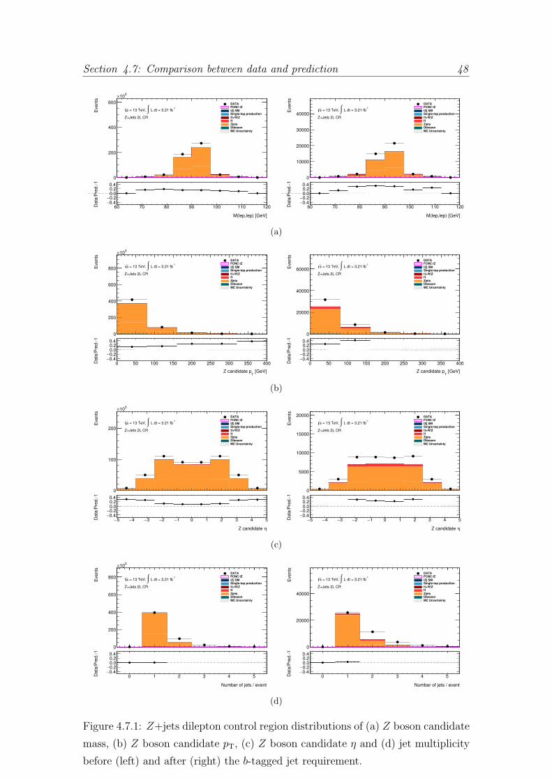
Section 4.7: Comparison between data and prediction 48
Eve
nts
0
200
400
600
310×
DATAFCNC tZtZj SMSingle-top production
+W|Ztttt
ZjetsDibosonMC Uncertainty
ATLAS
-1 L dt = 3.21 fb∫ = 13 TeV, s
Z+Jets 2L CR
M(lep,lep) [GeV]
60 70 80 90 100 110 120Da
ta/P
red
.-1
0.4−0.2−0.00.20.4
Eve
nts
0
10000
20000
30000
40000
DATAFCNC tZtZj SMSingle-top production
+W|Ztttt
ZjetsDibosonMC Uncertainty
ATLAS
-1 L dt = 3.21 fb∫ = 13 TeV, s
Z+Jets 2L CR
M(lep,lep) [GeV]
60 70 80 90 100 110 120Da
ta/P
red
.-1
0.4−0.2−0.00.20.4
(a)
Eve
nts
0
200
400
600
800
310×
DATAFCNC tZtZj SMSingle-top production
+W|Ztttt
ZjetsDibosonMC Uncertainty
ATLAS
-1 L dt = 3.21 fb∫ = 13 TeV, s
Z+Jets 2L CR
[GeV]T
Z candidate p
0 50 100 150 200 250 300 350 400Da
ta/P
red
.-1
0.4−0.2−0.00.20.4
Eve
nts
0
20000
40000
60000
DATAFCNC tZtZj SMSingle-top production
+W|Ztttt
ZjetsDibosonMC Uncertainty
ATLAS
-1 L dt = 3.21 fb∫ = 13 TeV, s
Z+Jets 2L CR
[GeV]T
Z candidate p
0 50 100 150 200 250 300 350 400Da
ta/P
red
.-1
0.4−0.2−0.00.20.4
(b)
Eve
nts
0
100
200
310×
DATAFCNC tZtZj SMSingle-top production
+W|Ztttt
ZjetsDibosonMC Uncertainty
ATLAS
-1 L dt = 3.21 fb∫ = 13 TeV, s
Z+Jets 2L CR
ηZ candidate
5− 4− 3− 2− 1− 0 1 2 3 4 5Da
ta/P
red
.-1
0.4−0.2−0.00.20.4
Eve
nts
0
5000
10000
15000
20000 DATAFCNC tZtZj SMSingle-top production
+W|Ztttt
ZjetsDibosonMC Uncertainty
ATLAS
-1 L dt = 3.21 fb∫ = 13 TeV, s
Z+Jets 2L CR
ηZ candidate
5− 4− 3− 2− 1− 0 1 2 3 4 5Da
ta/P
red
.-1
0.4−0.2−0.00.20.4
(c)
Eve
nts
0
200
400
600
800
310×
DATAFCNC tZtZj SMSingle-top production
+W|Ztttt
ZjetsDibosonMC Uncertainty
ATLAS
-1 L dt = 3.21 fb∫ = 13 TeV, s
Z+Jets 2L CR
Number of jets / event
0 1 2 3 4 5Da
ta/P
red
.-1
0.4−0.2−0.00.20.4
Eve
nts
0
20000
40000
DATAFCNC tZtZj SMSingle-top production
+W|Ztttt
ZjetsDibosonMC Uncertainty
ATLAS
-1 L dt = 3.21 fb∫ = 13 TeV, s
Z+Jets 2L CR
Number of jets / event
0 1 2 3 4 5Da
ta/P
red
.-1
0.4−0.2−0.00.20.4
(d)
Figure 4.7.1: Z+jets dilepton control region distributions of (a) Z boson candidate
mass, (b) Z boson candidate pT, (c) Z boson candidate η and (d) jet multiplicity
before (left) and after (right) the b-tagged jet requirement.

49 Section 4.7: Comparison between data and prediction
Eve
nts
0
500
1000
310×
DATAFCNC tZtZj SMSingle-top production
+W|Ztttt
ZjetsDibosonMC Uncertainty
ATLAS
-1 L dt = 3.21 fb∫ = 13 TeV, s
Z+Jets 2L CR
Number of bjets / event
0 1 2 3 4 5Da
ta/P
red
.-1
0.4−0.2−0.00.20.4
Eve
nts
0
20000
40000
60000
80000
DATAFCNC tZtZj SMSingle-top production
+W|Ztttt
ZjetsDibosonMC Uncertainty
ATLAS
-1 L dt = 3.21 fb∫ = 13 TeV, s
Z+Jets 2L CR
Number of bjets / event
0 1 2 3 4 5Da
ta/P
red
.-1
0.4−0.2−0.00.20.4
Figure 4.7.2: Z+jets dilepton control region distributions of b-tagged jet multi-
plicity before (left) and after (right) the b-tagged jet requirement.
Process Z+jets 2L CR
FCNC tZ 26.64± 0.60
SM tZj 19.23± 0.13
Single Top 141.74± 1.96
tt + W /Z 22.00± 0.08
tt 2 751.23± 15.43
Z + jets 29 064.40± 117.12
Dibosons 355.76± 4.74
Total background 32 354.37± 118.24
Observed 42 281
Table 4.7.2: Z+jets dilepton control region event yields after the selection criteria.
The uncertainties presented corresponds only to the statistical errors.
Analyzing the number of data events, the conclusion is that a not so good
agreement between data and prediction is obtained for this control region, specifi-
cally in the region with more than one jet. This difference in the number of events
can be explained by the Z+jets background normalisation that will be corrected
after a fit.

Section 4.7: Comparison between data and prediction 50
The selection of the Z+jets control region considering a trileptonic topology is the
same as for the dileptonic case but it requires exactly three leptons instead of two.
The control region considered here allows the study of the significance of the fakes
on the Z+jets processes since this process has only two leptons in the final state.
Figures 4.7.3 and 4.7.4 show some distributions for the trileptonic Z+jets control
region.
Figure 4.7.3(a) represents the Z boson candidate mass distribution with a peak
in the true value of the Z boson mass and a good agreement between data and
MC, even with a lot less events than the dileptonic Z+jets region. The pT distri-
bution shown in Figure 4.7.3(b) reveals again a softer distribution of background
compared with the signal. Figure 4.7.3(c) shows the Z boson candidate η where
a good agreement between data and MC exists before the b-tagging requirement
but not so good after. The jet multiplicity can be found in Figure 4.7.3(d) having
a big fraction of dibosons background what is expected since, in this topology,
the Z+jets will be characterized by fakes. However, the Z+jets background has
a reasonable number of events after all the selection criteria. The b-tagged jet
multiplicity distribution represented in Figure 4.7.4 shows a reasonable data and
MC agreement in both distributions. This agreement is a little better for the dis-
tributions after the b-tagging requirement. Due to the low statistics of this control
region, the number of events for signal increases while the number of the dom-
inant background (which corresponds to dibosons) decreases after the b-tagging
requirement.
The events yields for the control region of Z+jets background, in a trileptonic
topology, after the selection are shown in Table 4.7.3. Table 4.7.3 shows a not so
good isolation of Z+jets background where the dibosons is the dominant process.
However, the Z+jets is the third background with highest number of events, having
∼ 6 of the total of ∼ 37 background events. This behavior allows to conclude that
the fakes do not affect on a significant way this analysis since the processes with
three real leptons in the final state still dominate the background event yields.
A reasonable agreement between data and prediction is achieved even with a low
statistics after all the selection criteria for the control region considered.

51 Section 4.7: Comparison between data and prediction
Eve
nts
0
100
200
300
400DATAFCNC tZtZj SMSingle-top production
+W|Ztttt
ZjetsDibosonMC Uncertainty
ATLAS
-1 L dt = 3.21 fb∫ = 13 TeV, s
Z+Jets 3L CR
M(lep,lep) [GeV]
60 70 80 90 100 110 120Da
ta/P
red
.-1
0.4−0.2−0.00.20.4
Eve
nts
0
10
20
30
40 DATAFCNC tZtZj SMSingle-top production
+W|Ztttt
ZjetsDibosonMC Uncertainty
ATLAS
-1 L dt = 3.21 fb∫ = 13 TeV, s
Z+Jets 3L CR
M(lep,lep) [GeV]
60 70 80 90 100 110 120Da
ta/P
red
.-1
0.4−0.2−0.00.20.4
(a)
Eve
nts
0
100
200
300
400
DATAFCNC tZtZj SMSingle-top production
+W|Ztttt
ZjetsDibosonMC Uncertainty
ATLAS
-1 L dt = 3.21 fb∫ = 13 TeV, s
Z+Jets 3L CR
[GeV]T
Z candidate p
0 50 100 150 200 250 300 350 400Da
ta/P
red
.-1
0.4−0.2−0.00.20.4
Eve
nts
0
20
40
DATAFCNC tZtZj SMSingle-top production
+W|Ztttt
ZjetsDibosonMC Uncertainty
ATLAS
-1 L dt = 3.21 fb∫ = 13 TeV, s
Z+Jets 3L CR
[GeV]T
Z candidate p
0 50 100 150 200 250 300 350 400Da
ta/P
red
.-1
0.4−0.2−0.00.20.4
(b)
Eve
nts
0
50
100
150
200 DATAFCNC tZtZj SMSingle-top production
+W|Ztttt
ZjetsDibosonMC Uncertainty
ATLAS
-1 L dt = 3.21 fb∫ = 13 TeV, s
Z+Jets 3L CR
ηZ candidate
5− 4− 3− 2− 1− 0 1 2 3 4 5Da
ta/P
red
.-1
0.4−0.2−0.00.20.4
Eve
nts
0
10
20
DATAFCNC tZtZj SMSingle-top production
+W|Ztttt
ZjetsDibosonMC Uncertainty
ATLAS
-1 L dt = 3.21 fb∫ = 13 TeV, s
Z+Jets 3L CR
ηZ candidate
5− 4− 3− 2− 1− 0 1 2 3 4 5Da
ta/P
red
.-1
0.4−0.2−0.00.20.4
(c)
Eve
nts
0
200
400
DATAFCNC tZtZj SMSingle-top production
+W|Ztttt
ZjetsDibosonMC Uncertainty
ATLAS
-1 L dt = 3.21 fb∫ = 13 TeV, s
Z+Jets 3L CR
Number of jets / event
0 1 2 3 4 5Da
ta/P
red
.-1
0.4−0.2−0.00.20.4
Eve
nts
0
10
20
30
40DATAFCNC tZtZj SMSingle-top production
+W|Ztttt
ZjetsDibosonMC Uncertainty
ATLAS
-1 L dt = 3.21 fb∫ = 13 TeV, s
Z+Jets 3L CR
Number of jets / event
0 1 2 3 4 5Da
ta/P
red
.-1
0.4−0.2−0.00.20.4
(d)
Figure 4.7.3: Z+jets trilepton control region distributions of (a) Z boson candidate
mass, (b) Z boson candidate pT, (c) Z boson candidate η and (d) jet multiplicity
before (left) and after (right) the b-tagged jet requirement.

Section 4.7: Comparison between data and prediction 52
Eve
nts
0
200
400
600
DATAFCNC tZtZj SMSingle-top production
+W|Ztttt
ZjetsDibosonMC Uncertainty
ATLAS
-1 L dt = 3.21 fb∫ = 13 TeV, s
Z+Jets 3L CR
Number of bjets / event
0 1 2 3 4 5Da
ta/P
red
.-1
0.4−0.2−0.00.20.4
Eve
nts
0
20
40
60
80
DATAFCNC tZtZj SMSingle-top production
+W|Ztttt
ZjetsDibosonMC Uncertainty
ATLAS
-1 L dt = 3.21 fb∫ = 13 TeV, s
Z+Jets 3L CR
Number of bjets / event
0 1 2 3 4 5Da
ta/P
red
.-1
0.4−0.2−0.00.20.4
Figure 4.7.4: Z+jets trilepton control region distributions of b-tagged jet multi-
plicity before (left) and after (right) the b-tagged jet requirement.
Process Z+jets 3L CR
FCNC tZ 23.19± 0.56
SM tZj 4.67± 0.06
Single Top 0.14± 0.06
tt + W /Z 9.06± 0.05
tt 4.90± 0.64
Z + jets 6.28± 1.47
Dibosons 12.30± 0.25
Total background 37.36± 1.62
Observed 42
Table 4.7.3: Z+jets trilepton control region event yields after the selection criteria.
The uncertainties presented corresponds only to the statistical errors.
The tt control region selection requires exactly three leptons, EmissT higher than
20 GeV, MT(W ) higher than 40 GeV, at least one OSSF pair of leptons with a
reconstructed mass outside the range of 80 and 100 GeV and, finally, exactly two
jets where one is an b-tagged jet. Figure 4.7.5 shows relevant distributions of the
tt control region.
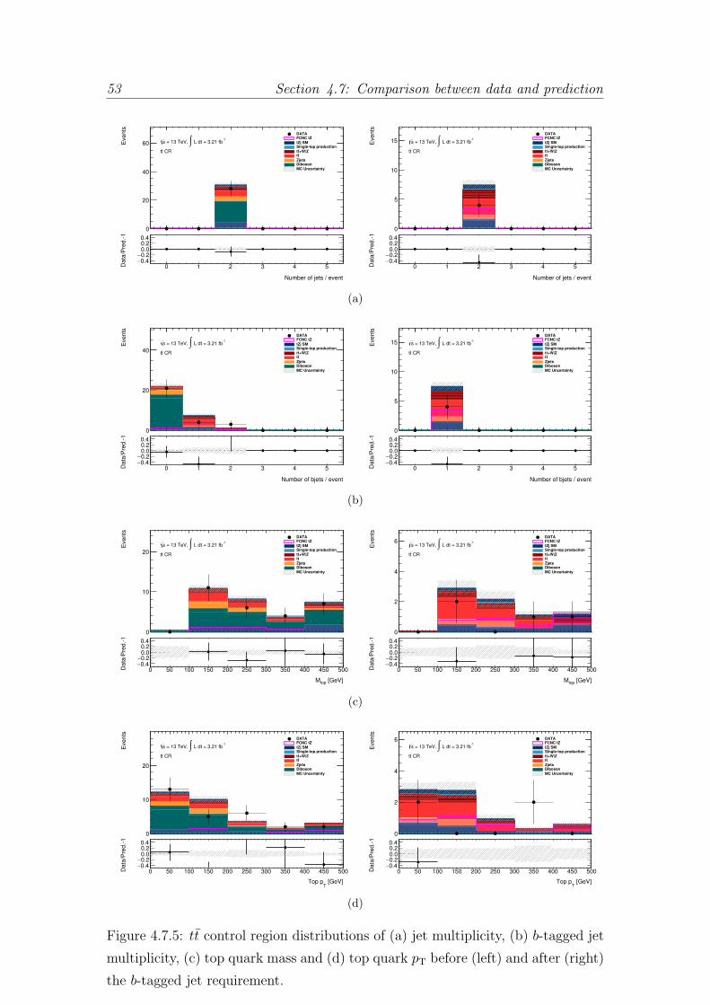
53 Section 4.7: Comparison between data and prediction
Eve
nts
0
20
40
60
DATAFCNC tZtZj SMSingle-top production
+W|Ztttt
ZjetsDibosonMC Uncertainty
ATLAS
-1 L dt = 3.21 fb∫ = 13 TeV, s
CRtt
Number of jets / event
0 1 2 3 4 5Da
ta/P
red
.-1
0.4−0.2−0.00.20.4
Eve
nts
0
5
10
15
DATAFCNC tZtZj SMSingle-top production
+W|Ztttt
ZjetsDibosonMC Uncertainty
ATLAS
-1 L dt = 3.21 fb∫ = 13 TeV, s
CRtt
Number of jets / event
0 1 2 3 4 5Da
ta/P
red
.-1
0.4−0.2−0.00.20.4
(a)
Eve
nts
0
20
40
DATAFCNC tZtZj SMSingle-top production
+W|Ztttt
ZjetsDibosonMC Uncertainty
ATLAS
-1 L dt = 3.21 fb∫ = 13 TeV, s
CRtt
Number of bjets / event
0 1 2 3 4 5Da
ta/P
red
.-1
0.4−0.2−0.00.20.4
Eve
nts
0
5
10
15
DATAFCNC tZtZj SMSingle-top production
+W|Ztttt
ZjetsDibosonMC Uncertainty
ATLAS
-1 L dt = 3.21 fb∫ = 13 TeV, s
CRtt
Number of bjets / event
0 1 2 3 4 5Da
ta/P
red
.-1
0.4−0.2−0.00.20.4
(b)
Eve
nts
0
10
20
DATAFCNC tZtZj SMSingle-top production
+W|Ztttt
ZjetsDibosonMC Uncertainty
ATLAS
-1 L dt = 3.21 fb∫ = 13 TeV, s
CRtt
[GeV]topM
0 50 100 150 200 250 300 350 400 450 500Da
ta/P
red
.-1
0.4−0.2−0.00.20.4
Eve
nts
0
2
4
6DATAFCNC tZtZj SMSingle-top production
+W|Ztttt
ZjetsDibosonMC Uncertainty
ATLAS
-1 L dt = 3.21 fb∫ = 13 TeV, s
CRtt
[GeV]topM
0 50 100 150 200 250 300 350 400 450 500Da
ta/P
red
.-1
0.4−0.2−0.00.20.4
(c)
Eve
nts
0
10
20
DATAFCNC tZtZj SMSingle-top production
+W|Ztttt
ZjetsDibosonMC Uncertainty
ATLAS
-1 L dt = 3.21 fb∫ = 13 TeV, s
CRtt
[GeV]T
Top p
0 50 100 150 200 250 300 350 400 450 500Da
ta/P
red
.-1
0.4−0.2−0.00.20.4
Eve
nts
0
2
4
6 DATAFCNC tZtZj SMSingle-top production
+W|Ztttt
ZjetsDibosonMC Uncertainty
ATLAS
-1 L dt = 3.21 fb∫ = 13 TeV, s
CRtt
[GeV]T
Top p
0 50 100 150 200 250 300 350 400 450 500Da
ta/P
red
.-1
0.4−0.2−0.00.20.4
(d)
Figure 4.7.5: tt control region distributions of (a) jet multiplicity, (b) b-tagged jet
multiplicity, (c) top quark mass and (d) top quark pT before (left) and after (right)
the b-tagged jet requirement.

Section 4.7: Comparison between data and prediction 54
Figure 4.7.5(a) represents the jet multiplicity before and after the b-tagging re-
quirement. The agreement between data and MC is reasonable for the distribu-
tion before requiring a b-tagged jet while is not good for the distribution after
this requirement. The same behavior is also observed in the distributions in Fig-
ure 4.7.5(b). The b-tagged jet multiplicity in Figure 4.7.5(b) shows the exclusion
power of the b-tagging requirement in the dibosons processes. After the selection
criteria, a reasonable fraction of tt events can be seen, even taking into account
that this process is characterized by having two and not three leptons in the final
state. Figure 4.7.5(c) represents the top quark reconstructed mass. The distribu-
tion shows a range of 100 and 500 GeV to this variable with a small peak in the
measured top quark mass (∼ 173 GeV). The pT distribution of the reconstructed
top quark shown in Figure 4.7.5(d) has a big range localized between 0 and 500
GeV. A good agreement between data and MC for the distributions in Figure 4.7.5
is disallowed by the low statistics in this region. Comparing the distributions for
the levels before and after the b-tagging requirement, a better agreement can be
seen in the distributions before this final criteria due to a higher statistics.
The events yields for the control region of tt background after the selection are
shown in Table 4.7.4. The event yields presented in Table 4.7.4 reveals that the
selection made for this control region was appropriate. The tt process is the
dominant background process having ∼ 3 of the ∼ 7 background events. However,
this region selection was defined taking in account the signal processes implying a
lack of statistics after the selection criteria. Despise that, a reasonable agreement
between data and MC was achieved considering the number of events after the
selection criteria. Through the event yields, a contamination of signal can be seen
due to the normalisation arbitrary chosen that was already excluded by the limits
obtained in previous searches [56, 57, 53, 55, 58].
The dibosons control region is focused on the WZ process since it is the dibosons
process closest to the signal final state. The selection consists in requiring exactly
three leptons, at least one OSSF pair of leptons with a reconstructed mass between
81 and 101 GeV and exactly one jet.

55 Section 4.7: Comparison between data and prediction
Process tt CR
FCNC tZ 3.45± 0.21
SM tZj 0.80± 0.03
Single Top 0.05± 0.03
tt + W /Z 1.54± 0.02
tt 2.81± 0.48
Z + jets 0.78± 0.55
Dibosons 1.54± 0.07
Total background 7.52± 0.73
Observed 4
Table 4.7.4: tt control region event yields after the selection criteria. The uncer-
tainties presented corresponds only to the statistical errors.
Figure 4.7.6 shows some relevant distributions for theWZ dibosons control region.
Figure 4.7.6(a) represents the W boson mass where a peak in the measured W
mass (∼ 80 GeV) can be seen. Besides that, it is clear that the dibosons is the
dominant background. Figure 4.7.6(b) shows the Z boson candidate mass with a
good agreement between data and MC and a peak in the region between 80 and
100 GeV. The pT distribution of the Z boson candidate in Figure 4.7.6(c) reveals
the main difference between the dibosons background and the signal. While the
dibosons events has a softer pT distribution, the signal has a harder distribution.
This characteristic can be used to separate background and signal in the next step
of this analysis. A good agreement between data and prediction is also achieved
in these distributions. The b-tagged jet multiplicity represented in Figure 4.7.6(d)
shows again that the signal events are characterized by having a b-tagged jet
in the final state and the majority of events are localized in the region without
a b-tagged jet which is important to distinguish signal from background. Figure
4.7.6(e) represents the distribution for the transverse mass of theW boson showing
that the signal and the dibosons background have similar distributions for this

Section 4.7: Comparison between data and prediction 56
observable. This characteristic can be predicted since one W boson is expected in
both final states. A good agreement between data and MC is a characteristic of
the distributions for this control region.
The same behavior is seen in Figure 4.7.6(f) where the EmissT distribution is shown.
Both the signal and the dibosons background has a distribution composed by high
values of EmissT which is consistent with at least one neutrino in the final state.
Knowing that the W boson can decay to a charged lepton and a neutrino, this
distribution is consistent with the prediction.
The events yields for the control region of dibosons background, specifically in the
WZ process, after the selection are shown in Table 4.7.5.
The good isolation of the WZ dibosons processes in this control region can be
seen in Table 4.7.5 where the dibosons background has ∼ 125 against the total of
∼ 133 background events. The agreement between data and MC is not so good
and can be explain by the Z+jets normalisation. A fit can be helpful for a better
agreement between data and MC. Since the dibosons is the dominant background
of the signal region, the distributions for this control region allows the study of
possible discriminant variables.
The tZj control region definition is important since this process has a topology
similar to the signal region. The tZj process has a small cross-section expectation
and no evidence was found until the moment [58]. The selection requires exactly
three leptons, EmissT higher than 20 GeV, at least one OSSF pair of leptons having
a mass between 70 and 110 GeV and at least one jet having exactly one b-tagged
jet.
Figure 4.7.7 shows some relevant distributions for the tZj control region. The
jet multiplicity represented in Figure 4.7.7(a) shows the effect that the b-tagging
requirement has in this control region. Before requiring an b-tagged jet the main
background corresponds to the dibosons processes. However, after the b-tagging
requirement, the total background is composed by the different backgrounds con-
sidered but in small fractions. The data and MC agreement is reasonable for both
the distributions in the regions between one and three jets where the majority of
the number of events is observed.

57 Section 4.7: Comparison between data and prediction
Eve
nts
1−10
1
10
210
DATAFCNC tZtZj SMSingle-top production
+W|Ztttt
ZjetsDibosonMC Uncertainty
ATLAS
-1 L dt = 3.21 fb∫ = 13 TeV, s
WZ Diboson CR
[GeV]W
M
0 20 40 60 80 100 120 140Da
ta/P
red
.-1
0.4−0.2−0.00.20.4
(a)
Eve
nts
1−10
1
10
210
DATAFCNC tZtZj SMSingle-top production
+W|Ztttt
ZjetsDibosonMC Uncertainty
ATLAS
-1 L dt = 3.21 fb∫ = 13 TeV, s
WZ Diboson CR
M(lep,lep) [GeV]
60 70 80 90 100 110 120Da
ta/P
red
.-1
0.4−0.2−0.00.20.4
(b)
Eve
nts
10
210
DATAFCNC tZtZj SMSingle-top production
+W|Ztttt
ZjetsDibosonMC Uncertainty
ATLAS
-1 L dt = 3.21 fb∫ = 13 TeV, s
WZ Diboson CR
[GeV]T
Z candidate p
0 50 100 150 200 250 300 350 400Da
ta/P
red
.-1
0.4−0.2−0.00.20.4
(c)
Eve
nts
1
10
210
DATAFCNC tZtZj SMSingle-top production
+W|Ztttt
ZjetsDibosonMC Uncertainty
ATLAS
-1 L dt = 3.21 fb∫ = 13 TeV, s
WZ Diboson CR
Number of bjets / event
0 1 2 3 4 5Da
ta/P
red
.-1
0.4−0.2−0.00.20.4
(d)
Eve
nts
1
10
210
DATAFCNC tZtZj SMSingle-top production
+W|Ztttt
ZjetsDibosonMC Uncertainty
ATLAS
-1 L dt = 3.21 fb∫ = 13 TeV, s
WZ Diboson CR
[GeV]T, W
M
0 50 100 150 200 250Da
ta/P
red
.-1
0.4−0.2−0.00.20.4
(e)
Eve
nts
1
10
210DATAFCNC tZtZj SMSingle-top production
+W|Ztttt
ZjetsDibosonMC Uncertainty
ATLAS
-1 L dt = 3.21 fb∫ = 13 TeV, s
WZ Diboson CR
[GeV]miss
TE
0 50 100 150 200 250 300Da
ta/P
red
.-1
0.4−0.2−0.00.20.4
(f)
Figure 4.7.6: WZ Diboson control region distributions of (a) W boson mass, (b)
Z boson candidate mass, (c) Z boson candidate pT, (d) b-tagged jet multiplicity,
(e) W boson transverse mass and (f) EmissT after the selection criteria.

Section 4.7: Comparison between data and prediction 58
Process WZ Diboson CR
FCNC tZ 4.41± 0.25
SM tZj 1.01± 0.03
Single Top 0.03± 0.03
tt + W /Z 0.40± 0.01
tt 0.75± 0.25
Z + jets 5.85± 1.64
Dibosons 125.45± 0.63
Total background 133.50± 1.77
Observed 151
Table 4.7.5: WZ Diboson control region event yields after the selection criteria.
The uncertainties presented corresponds only to the statistical errors.
Figure 4.7.7(b) represents the b-tagged jet multiplicity distributions. Before re-
quiring a b-tagged jet, a reasonable agreement between data and MC is seen in the
region without b-jets and with exactly one b-jet. After requiring one b-jet, a bet-
ter agreement between data and MC was achieved where the tZj SM background
starts to appears along with the other backgrounds processes. Figure 4.7.7(c)
shows the Z boson candidate mass distribution with a reasonable data and MC
agreement being better in the region between 80 and 100 GeV due to the large
statistics. Comparing the two distributions, it is clear the effect that the b-tagging
requirement has in the number of events of background decreasing a factor of ∼10.
The EmissT distributions in Figure 4.7.7(d) show a similar behavior between the
signal and the main background which corresponds to the dibosons background.
This behavior is characterized by high values of EmissT which is consistent with the
signal and the dibosons background prediction. Since a W boson is a characteris-
tic of these two processes, a neutrino is expected in the final state leading to high
values of the variable EmissT .

59 Section 4.7: Comparison between data and prediction
Eve
nts
0
200
400
600
800DATAFCNC tZtZj SMSingle-top production
+W|Ztttt
ZjetsDibosonMC Uncertainty
ATLAS
-1 L dt = 3.21 fb∫ = 13 TeV, s
tZj SM CR
Number of jets / event
0 1 2 3 4 5Da
ta/P
red
.-1
0.4−0.2−0.00.20.4
Eve
nts
0
10
20
30 DATAFCNC tZtZj SMSingle-top production
+W|Ztttt
ZjetsDibosonMC Uncertainty
ATLAS
-1 L dt = 3.21 fb∫ = 13 TeV, s
tZj SM CR
Number of jets / event
0 1 2 3 4 5Da
ta/P
red
.-1
0.4−0.2−0.00.20.4
(a)
Eve
nts
0
500
1000DATAFCNC tZtZj SMSingle-top production
+W|Ztttt
ZjetsDibosonMC Uncertainty
ATLAS
-1 L dt = 3.21 fb∫ = 13 TeV, s
tZj SM CR
Number of bjets / event
0 1 2 3 4 5Da
ta/P
red
.-1
0.4−0.2−0.00.20.4
Eve
nts
0
20
40
60
80DATAFCNC tZtZj SMSingle-top production
+W|Ztttt
ZjetsDibosonMC Uncertainty
ATLAS
-1 L dt = 3.21 fb∫ = 13 TeV, s
tZj SM CR
Number of bjets / event
0 1 2 3 4 5Da
ta/P
red
.-1
0.4−0.2−0.00.20.4
(b)
Eve
nts
0
100
200
300 DATAFCNC tZtZj SMSingle-top production
+W|Ztttt
ZjetsDibosonMC Uncertainty
ATLAS
-1 L dt = 3.21 fb∫ = 13 TeV, s
tZj SM CR
M(lep,lep) [GeV]
60 70 80 90 100 110 120Da
ta/P
red
.-1
0.4−0.2−0.00.20.4
Eve
nts
0
10
20
30
DATAFCNC tZtZj SMSingle-top production
+W|Ztttt
ZjetsDibosonMC Uncertainty
ATLAS
-1 L dt = 3.21 fb∫ = 13 TeV, s
tZj SM CR
M(lep,lep) [GeV]
60 70 80 90 100 110 120Da
ta/P
red
.-1
0.4−0.2−0.00.20.4
(c)
Eve
nts
10
210
DATAFCNC tZtZj SMSingle-top production
+W|Ztttt
ZjetsDibosonMC Uncertainty
ATLAS
-1 L dt = 3.21 fb∫ = 13 TeV, s
tZj SM CR
[GeV]miss
TE
0 50 100 150 200 250 300Da
ta/P
red
.-1
0.4−0.2−0.00.20.4
Eve
nts
1−10
1
10
DATAFCNC tZtZj SMSingle-top production
+W|Ztttt
ZjetsDibosonMC Uncertainty
ATLAS
-1 L dt = 3.21 fb∫ = 13 TeV, s
tZj SM CR
[GeV]miss
TE
0 50 100 150 200 250 300Da
ta/P
red
.-1
0.4−0.2−0.00.20.4
(d)
Figure 4.7.7: tZj control region distributions of (a) jet multiplicity, (b) b-tagged
jet multiplicity, (c) Z boson candidate mass and (d) EmissT before (left) and after
(right) the b-tagged jet requirement.
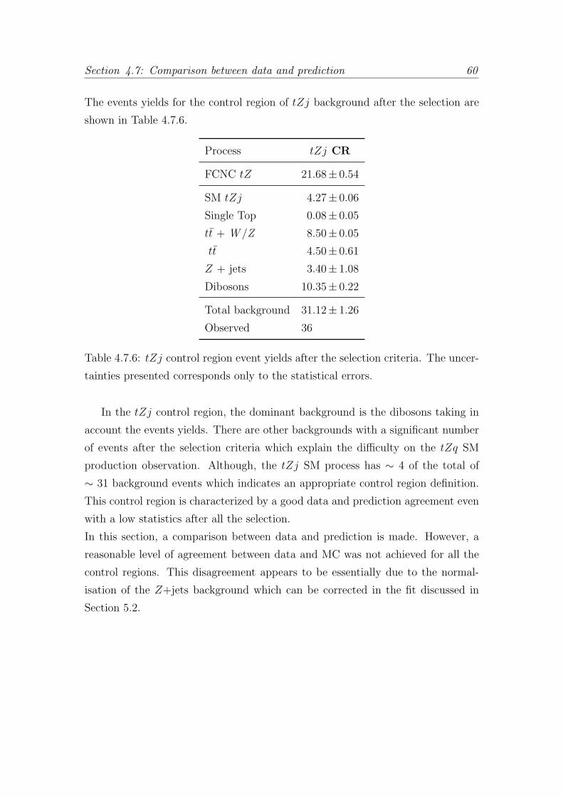
Section 4.7: Comparison between data and prediction 60
The events yields for the control region of tZj background after the selection are
shown in Table 4.7.6.
Process tZj CR
FCNC tZ 21.68± 0.54
SM tZj 4.27± 0.06
Single Top 0.08± 0.05
tt + W /Z 8.50± 0.05
tt 4.50± 0.61
Z + jets 3.40± 1.08
Dibosons 10.35± 0.22
Total background 31.12± 1.26
Observed 36
Table 4.7.6: tZj control region event yields after the selection criteria. The uncer-
tainties presented corresponds only to the statistical errors.
In the tZj control region, the dominant background is the dibosons taking in
account the events yields. There are other backgrounds with a significant number
of events after the selection criteria which explain the difficulty on the tZq SM
production observation. Although, the tZj SM process has ∼ 4 of the total of
∼ 31 background events which indicates an appropriate control region definition.
This control region is characterized by a good data and prediction agreement even
with a low statistics after all the selection.
In this section, a comparison between data and prediction is made. However, a
reasonable level of agreement between data and MC was not achieved for all the
control regions. This disagreement appears to be essentially due to the normal-
isation of the Z+jets background which can be corrected in the fit discussed in
Section 5.2.
61 Section 4.9: Systematic uncertainties
4.8 Systematic uncertainties
The presented results are affected by different sources of systematic uncertainties
associated with the respective measurement and that include the background and
signal modeling as well as the instrumental uncertainties. The sources studied
in this thesis include the measurement of the luminosity, lepton efficiency scale
factor, lepton energy scale and resolution, jet energy scale and resolution, the b-
tagging efficiency and EmissT calculation. These uncertainties are propagated to the
analysis by varying the corresponding parameters in the event reconstruction and
repeating the full analysis. The resulting event yields can then be compared to
the central values obtained with the nominal event reconstruction in order to get
an estimate of the effect of the systematic uncertainty.
Uncertainties like the b-tagging efficiency and the jet energy scale are split into
several components representing independent uncertainties. The dominant sources
of uncertainty are due to the jet energy scale and resolution. The jet energy scale
uncertainty is divided in orthogonal components which represent independent ef-
fective uncertainties using different techniques. The jet energy resolution uncer-
tainty is obtained through comparisons of simulation and data using studies with
Run-1 data. These studies are then checked to have an agreement with Run-2
data [97].
The EmissT calculation consists in contributions from soft terms coming from low-pT
pileup jets and underlying event activity and from hard terms coming from leptons
and jets. The uncertainty related with the soft terms is obtained by comparing
the simulated scale and resolution to that in data. The uncertainty associated
with the hard terms is propagated from the corresponding jet and lepton scale
and resolution uncertainties being classified together with the uncertainty on the
hard objects.
The b-tagging uncertainties are determined with the√s= 8 TeV data, then ex-
trapolated and checked using the√s= 13 TeV data. These uncertainties use
independent eigenvectors for the efficiency of b jets, c jets, light-parton jets and
two extrapolation uncertainty factors.

Section 4.9: Discriminant variables 62
4.9 Discriminant variables
The separation of background and signal can be found through a study of possible
discriminant variables. In Section 4.6.1, the signal region selection was presented
and the conclusion is that the pT distribution of the Z boson candidate corresponds
to the best variable to distinguish signal from background. Since the dominant
backgrounds of this analysis corresponds to the dibosons and Z+jets processes,
the final state of these processes can be used to study the relation between the
distributions of pT of the Z boson candidate with the reconstructed top quark
mass and with the transverse mass of the reconstructed W boson. The Z+jets
background was a final state with a reconstructed Z boson and jets. This process
does not contain a top quark or aW boson which means that the reconstructed top
quark mass should not peak in the top quark mass and the transverse mass of the
reconstructed W boson should have values below 50 GeV. The dominant process
of the dibosons background is the WZ process. This means that the transverse
mass of the W boson should be higher than 50 GeV with the same behavior of the
signal process. Since a top quark is not expected in the final state, it is expected
that the reconstructed top quark mass do not have a distribution compatible with
the mass distribution of a top quark. In Figures 4.9.1 and 4.9.2, a comparison for
backgrounds and signal of two dimensional distributions of the pT of the Z boson
candidate with the reconstructed top quark mass and the transverse mass of the
W boson after the signal region selection was presented.
Figure 4.9.1(a) shows the distributions for the single top background where the
production of one top quark is expected. Since in this analysis only theWt channel
are studied for the single top production, the final state consists in a top quark and
a W boson. The distributions shown in Figure 4.9.1(a) reveals a good description
of the background process studied.
Concerning the tt background distributions, represented in Figure 4.9.1(b), the
transverse mass of the W boson was distributed in all the range (between 0 and
250 GeV). This behavior only can be seen in these background process.

63 Section 4.9: Discriminant variables
M(top) [GeV]
0100
200300
400500
[GeV]T
Z candidate p
0100
200300
400
Events
0
500
1000
Single Top
[GeV]T,WM
050
100150
200250
[GeV]T
Z candidate p
0100
200300
400
Events
0
200
400
600
800
Single Top
(a)
M(top) [GeV]
0100
200300
400500
[GeV]T
Z candidate p
0100
200300
400
Events
0
200
400
600
800
tt
[GeV]T,WM
050
100150
200250
[GeV]T
Z candidate p
0100
200300
400
Events
0
200
400
600
tt
(b)
M(top) [GeV]0
100200
300400
500
[GeV]T
Z candidate p0
100200
300400
Events
0
1000
2000
3000
Dibosons
[GeV]T,WM
050
100150
200250
[GeV]T
Z candidate p0
100200
300400
Events
0
1000
2000
3000
Dibosons
(c)
Figure 4.9.1: Two dimensional distributions for (a) single top production, (b)
tt and (c) dibosons, shown as a function of the Z boson candidate pT and the
reconstructed top quark mass (left) and the transverse mass of theW boson (right).

Section 4.9: Discriminant variables 64
M(top) [GeV]
0100
200300
400500
[GeV]T
Z candidate p
0100
200300
400
Events
0
10000
20000
+jetsZ
[GeV]T,WM
050
100150
200250
[GeV]T
Z candidate p
0100
200300
400
Events
0
10000
20000
+jetsZ
(a)
M(top) [GeV]
0100
200300
400500
[GeV]T
Z candidate p
0100
200300
400
Events
0
50
100
150
Signal
[GeV]T,WM
050
100150
200250
[GeV]T
Z candidate p
0100
200300
400
Events
0
50
100
150
Signal
(b)
Figure 4.9.2: Two dimensional distributions for (a) Z + Jets and (b) signal, shown
as function of the Z boson candidate pT and the reconstructed top quark mass
(left) and the transverse mass of the W boson (right).
In Figure 4.9.1(c) are represented the dibosons background distributions with the
a higher number of events in the region with a transverse mass ofW boson between
50 and 100 GeV.
In Figure 4.9.2(a) for the Z+jets, the two dimensional distributions shows that all
the events have a transverse mass of the W boson lower than 50 GeV, implying
that this a good variable to cut on the signal region selection.
The distributions for signal, in Figure 4.9.2(b), show the majority of events in
the region with the MT(W ) higher than 50 GeV which are in agreement with the
presence of a W boson in the final state.

65 Section 4.9: Discriminant variables
For all the background and signal distributions, the number of events is signifi-
cantly higher in the region of the reconstructed top quark mass between 100 and
200 GeV (which are in agreement with the measured top quark mass of 173 GeV).
These two dimensional distributions comparing the Z boson candidate pT with
the reconstructed top quark mass shows that maybe the top quark mass is not a
good discriminant variable.
In order to study the effect of this two variables, new signal regions are defined
where one cut is added to the signal region selection. The goal is to have two sets
of complementary regions. The first set is characterized for having a cut on the
transverse mass of the W boson with one region requiring a value below 50 GeV
and the complementary region above 50 GeV. The second set has a cut on the
reconstructed top quark mass where the reconstructed top quark mass should be
inside or outside a range of 153 and 193 GeV (difference of 20 GeV to the measured
top quark mass which is 173 GeV [5]).
SR MT(W )<50 GeV SR MT(W )>50 GeV SR On top peak SR Off top peak
= 3 leptons
≥ 1 OSSF Pair
70 GeV < M(ℓℓ) < 110 GeV
= 1 b-tagged jet
MT(W ) < 50 GeV MT(W ) > 50 GeV |Mreco(t)−M(t)| < 20 GeV |Mreco(t)−M(t)| > 20 GeV
Table 4.9.1: Definition of distinct signal region selections in order to separate back-
ground for signal. A cut on the transverse mass ofW boson or in the reconstructed
top quark mass are added to the signal region selection.
The distributions of the two regions with the added cut on the transverse mass of
W boson are shown in Figure 4.9.3. With this cut, the expectation is to separate
the Z+jets background from all the other backgrounds and signal.
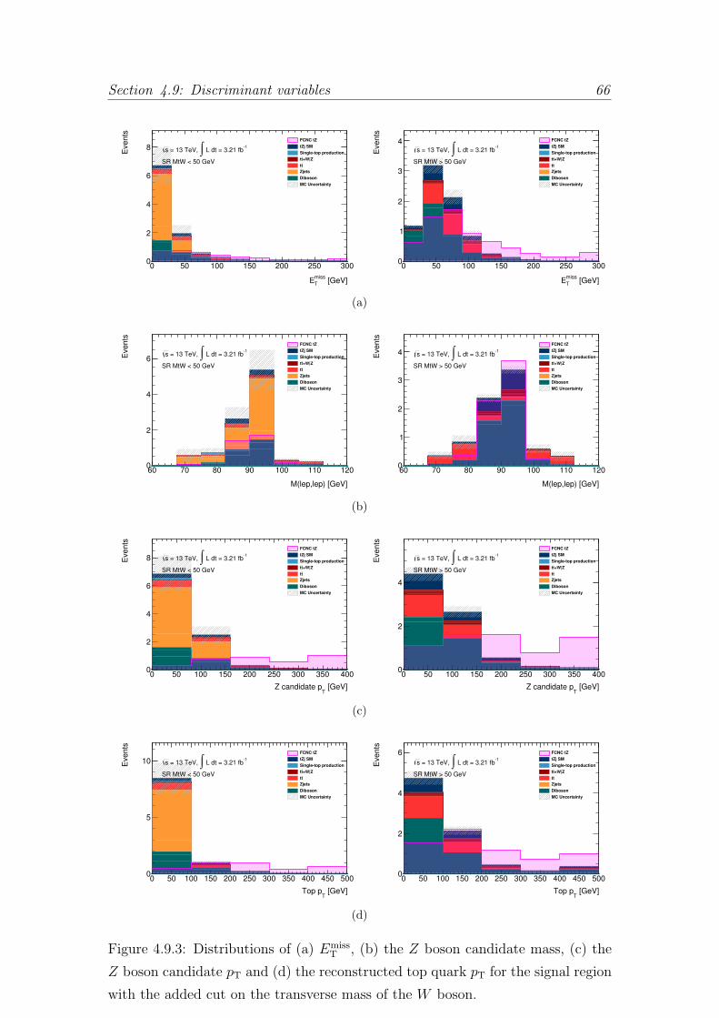
Section 4.9: Discriminant variables 66
[GeV]miss
TE
0 50 100 150 200 250 300
Events
0
2
4
6
8FCNC tZ
tZj SM
Single-top production
+W|Ztt
tt
Zjets
Diboson
MC Uncertainty
-1 L dt = 3.21 fb∫ = 13 TeV, s
SR MtW < 50 GeV
[GeV]miss
TE
0 50 100 150 200 250 300
Events
0
1
2
3
4 FCNC tZ
tZj SM
Single-top production
+W|Ztt
tt
Zjets
Diboson
MC Uncertainty
-1 L dt = 3.21 fb∫ = 13 TeV, s
SR MtW > 50 GeV
(a)
M(lep,lep) [GeV]
60 70 80 90 100 110 120
Events
0
2
4
6
FCNC tZ
tZj SM
Single-top production
+W|Ztt
tt
Zjets
Diboson
MC Uncertainty
-1 L dt = 3.21 fb∫ = 13 TeV, s
SR MtW < 50 GeV
M(lep,lep) [GeV]
60 70 80 90 100 110 120
Events
0
1
2
3
4FCNC tZ
tZj SM
Single-top production
+W|Ztt
tt
Zjets
Diboson
MC Uncertainty
-1 L dt = 3.21 fb∫ = 13 TeV, s
SR MtW > 50 GeV
(b)
[GeV]T
Z candidate p
0 50 100 150 200 250 300 350 400
Events
0
2
4
6
8
FCNC tZ
tZj SM
Single-top production
+W|Ztt
tt
Zjets
Diboson
MC Uncertainty
-1 L dt = 3.21 fb∫ = 13 TeV, s
SR MtW < 50 GeV
[GeV]T
Z candidate p
0 50 100 150 200 250 300 350 400
Events
0
2
4
FCNC tZ
tZj SM
Single-top production
+W|Ztt
tt
Zjets
Diboson
MC Uncertainty
-1 L dt = 3.21 fb∫ = 13 TeV, s
SR MtW > 50 GeV
(c)
[GeV]T
Top p
0 50 100 150 200 250 300 350 400 450 500
Events
0
5
10
FCNC tZ
tZj SM
Single-top production
+W|Ztt
tt
Zjets
Diboson
MC Uncertainty
-1 L dt = 3.21 fb∫ = 13 TeV, s
SR MtW < 50 GeV
[GeV]T
Top p
0 50 100 150 200 250 300 350 400 450 500
Events
0
2
4
6 FCNC tZ
tZj SM
Single-top production
+W|Ztt
tt
Zjets
Diboson
MC Uncertainty
-1 L dt = 3.21 fb∫ = 13 TeV, s
SR MtW > 50 GeV
(d)
Figure 4.9.3: Distributions of (a) EmissT , (b) the Z boson candidate mass, (c) the
Z boson candidate pT and (d) the reconstructed top quark pT for the signal region
with the added cut on the transverse mass of the W boson.

67 Section 4.9: Discriminant variables
The plots in Figure 4.9.3 reflects the excellent isolation of the Z+jets background
in the region with the transverse mass of the W boson below 50 GeV which is
the second dominant background of the signal region. More specifically the EmissT
distribution in Figure 4.9.3(a) shows the clear signature of signal when the cut of
MT(W ) > 50 GeV is applied. Beside that, the Z+jets background has the lowest
values of this variable in agreement with the final state of this process.
In Figure 4.9.3(b) the Z boson candidate mass is characterized by a good distribu-
tion in the two regions with a peak centered in the Z boson measured mass. This
behavior does not allow the possibility of considering the Z mass as a discriminant
variable. The pT of the Z boson candidate and the reconstructed top quark mass
can be considered as discriminant variables due to the differences between signal
and background distributions shown in Figures 4.9.3(c) and 4.9.3(d).
The event yields for these two complementary regions, in Table 4.9.2, reveals once
again the excellent isolation of the Z+jets with all the events from this background
in the region with the MT(W ) lower than 50 GeV. The single top background
corresponding to the Wt channel are also isolated in the region with the lower
MT(W ). However, the dibosons processes still have the higher fraction of the
background event yields.
The distributions of the two regions with the added cut on the reconstructed top
quark mass are shown in Figure 4.9.4. With this cut, the expectation is also
separate the Z+jets background from all the other backgrounds and signal since
this process do not have a top quark in the final state.

Section 4.9: Discriminant variables 68
Process SR SR
MT(W ) <50 MT(W )>50
FCNC tZ 3.47± 0.22 6.62± 0.30
SM tZj 0.62± 0.02 1.32± 0.03
Single Top 0.08± 0.05 0.00± 0.00
tt + W /Z 0.23± 0.01 0.53± 0.01
tt 0.71± 0.24 1.64± 0.38
Z + jets 5.47± 1.35 0.00± 0.00
Dibosons 2.66± 0.17 4.34± 0.12
Total background 9.80± 1.38 7.84± 0.40
Table 4.9.2: Event yields for the signal region selection with a cut on the transverse
mass of the reconstructed W boson. The uncertainties presented corresponds only
to the statistical errors.
The EmissT distribution, in Figure 4.9.4(a), shows a higher percentage of tt, dibosons
and other backgrounds in the region inside the top quark mass and a higher per-
centage of Z+jets in the region outside the top quark mass. The signal simulation
has higher values of EmissT in the region inside the top quark mass in agreement
with the prediction since a neutrino are expected in the final state.
In Figure 4.9.4(b) are shown the Z boson candidate mass distribution in agreement
with the prediction and well defined around the measured value of the Z boson.
The Z boson candidate pT represented in Figure 4.9.4(c) reveals a promising dis-
tribution which is different for background and signal. The same behavior can be
seen in Figure 4.9.4(d) where the reconstructed top quark mass are shown. For
these distributions, the background processes have a softer distribution while the
signal has a harder pT values. In agreement with Figure 4.9.3(c), the Z boson
candidate pT probes again being a good discriminant variable.

69 Section 4.9: Discriminant variables
[GeV]miss
TE
0 50 100 150 200 250 300
Events
0
0.5
1
1.5
2FCNC tZ
tZj SM
Single-top production
+W|Ztt
tt
Zjets
Diboson
MC Uncertainty
-1 L dt = 3.21 fb∫ = 13 TeV, s
SR On top peak
[GeV]miss
TE
0 50 100 150 200 250 300
Events
0
2
4
6
8 FCNC tZ
tZj SM
Single-top production
+W|Ztt
tt
Zjets
Diboson
MC Uncertainty
-1 L dt = 3.21 fb∫ = 13 TeV, s
SR Off top peak
(a)
M(lep,lep) [GeV]
60 70 80 90 100 110 120
Events
0
0.5
1
1.5
2FCNC tZ
tZj SM
Single-top production
+W|Ztt
tt
Zjets
Diboson
MC Uncertainty
-1 L dt = 3.21 fb∫ = 13 TeV, s
SR On top peak
M(lep,lep) [GeV]
60 70 80 90 100 110 120
Events
0
2
4
6
8
FCNC tZ
tZj SM
Single-top production
+W|Ztt
tt
Zjets
Diboson
MC Uncertainty
-1 L dt = 3.21 fb∫ = 13 TeV, s
SR Off top peak
(b)
[GeV]T
Z candidate p
0 50 100 150 200 250 300 350 400
Events
0
1
2
3FCNC tZ
tZj SM
Single-top production
+W|Ztt
tt
Zjets
Diboson
MC Uncertainty
-1 L dt = 3.21 fb∫ = 13 TeV, s
SR On top peak
[GeV]T
Z candidate p
0 50 100 150 200 250 300 350 400
Events
0
5
10
FCNC tZ
tZj SM
Single-top production
+W|Ztt
tt
Zjets
Diboson
MC Uncertainty
-1 L dt = 3.21 fb∫ = 13 TeV, s
SR Off top peak
(c)
[GeV]T
Top p
0 50 100 150 200 250 300 350 400 450 500
Events
0
1
2
3
FCNC tZ
tZj SM
Single-top production
+W|Ztt
tt
Zjets
Diboson
MC Uncertainty
-1 L dt = 3.21 fb∫ = 13 TeV, s
SR On top peak
[GeV]T
Top p
0 50 100 150 200 250 300 350 400 450 500
Events
0
5
10
FCNC tZ
tZj SM
Single-top production
+W|Ztt
tt
Zjets
Diboson
MC Uncertainty
-1 L dt = 3.21 fb∫ = 13 TeV, s
SR Off top peak
(d)
Figure 4.9.4: Distributions of (a) EmissT , (b) the Z boson candidate mass, (c) the
Z boson candidate pT and (d) the reconstructed top quark pT for the signal region
with the added cut on the reconstructed top quark mass.

Section 4.9: Discriminant variables 70
Process SR SR
On top peak Off top peak
FCNC tZ 3.95± 0.23 6.15± 0.29
SM tZj 0.89± 0.03 1.05± 0.03
Single Top 0.03± 0.03 0.06± 0.04
tt + W /Z 0.17± 0.01 0.60± 0.01
tt 0.69± 0.24 1.67± 0.38
Z + jets 0.66± 0.42 4.81± 1.28
Dibosons 1.38± 0.06 5.62± 0.20
Total background 3.82± 0.49 13.81± 1.35
Table 4.9.3: Event yields for the signal region selection with a cut on the recon-
structed top quark mass. The uncertainties presented corresponds only to the
statistical errors.
The events yields for the two regions with the cut on the reconstructed top quark
mass, in Table 4.9.3, reveals that the majority of events passed the selection with
the reconstructed quark mass outside the top peak. However, a reasonable isolation
of the Z+jets background are obtained with ∼ 90% of the events selected by the
region with the top quark mass outside the mass peak.

Chapter 5
Limits
Through the CLs prescription at the 95% CL, expected upper limits on the tZ
production via FCNC cross-section was obtained. With these limits on the cross-
section, expected limits on the branching ratios can be defined. In this chapter
a briefly description of the CLs method [98, 99] and the limits on the anomalous
coupling and the branching ratio are presented.
5.1 The CLs method
In particle physics one of the most important goals of a search is to exclude as much
as possible the existence of a signal in its absence or to confirm the existence of a
true signal as much as possible. The discovery or exclusion of a new physics model
is performed trough a statistical test. In order to achieve this, two hypothesis are
considered and tested where one describes the known physics processes and the
other includes the new phenomena. These two scenarios are described as follows:
• Corresponding to the SM known processes, it is often referred to as the
background-only (b) hypothesis;
• Corresponding to the SM known processes with the addition of a new signal
process, it is often referred to as the signal-plus-background (s+b) hypothesis.
71
Section 5.1: The CLs method 72
In the search presented in this thesis, the SM without FCNC interactions is con-
sidered the background-only scenario, while the signal-plus-background scenario
includes the FCNC interactions as signal.
A test statistical Q is used to quantify the compatibility of the observed data
with the given hypothesis being optimal when it is the likelihood ratio of Poisson
probabilities as follows
Q =P (data|signal + background)
P (data|background) (5.1.1)
where the probabilities are defined as
P (data|background) = bne−b
n!(5.1.2)
P (data|signal + background) =(s+ b)ne−(s+b)
n!(5.1.3)
being s and b the signal and background expected events after an analysis and n
the observed number of events.
The consistency of the data with the background-only and the signal-plus-background
hypothesis is obtained through a association between the test statistic Q and the
probability distribution P . These consistencies are obtained by defining different
confidence levels.
The confidence level for excluding the possibility of simultaneous presence of new
interactions or new particles production and background (s+b hypothesis) is given
by CLs+b and can be defined as the probability that the test statistic would be less
than or equal to that observed in the data, assuming the presence of both signal
and background. The confidence level for the background alone is given by CLb
and can be defined as the probability that background processes would give fewer
than or equal to the number of candidates observed. These two confidence levels
are defined as follows
CLs+b = P (Q ≤ Qobs|signal + background) (5.1.4)
CLb = P (Q ≤ Qobs|background) (5.1.5)
With the CLs+b and CLb defined, the equation of the confidence level for the
73 Section 5.2: Limits on the tZ production
signal-only hypothesis, CLs, can be obtained and defined as
CLs =CLs+b
CLb
. (5.1.6)
In case CLs < 0.05, the signal-plus-background hypothesis with a signal strength
µ is excluded at 95% CL. Taking in account that the number of expected signal
events s depends on the expected cross-section or other model parameters, the
upper or lower limits for the different values can be computed. Specifically in
the cross-section, upper limits on the expected cross-section can be obtained by
solving the equation
CLs(σ) = α (5.1.7)
with the fixed value of α is defined on the chosen confidence level (1 - α).
5.2 Limits on the tZ production
The study of possible discriminant variables in Section 4.8 enabled the definition
of the transverse mass of the W boson as the discriminant variable used for this
analysis. Through a fit in the two complementary signal regions with a cut on the
MT(W ) (selection defined in Table 4.9.1), expected upper limits are obtained for
a luminosity of 3.21 fb−1 and 30 fb−1.
The calculation of the limits for tZ production via FCNC presented here have
been made in collaboration with the Humboldt University of Berlin. To obtain the
limits presented here, different fits have been performed. First, a fit background-
only model to real data was made. After this, using the nuisance parameters from
the fit, a Asimov dataset without signal was generated. The expected upper limits
was determined and a new Asimov dataset with signal set to the upper limit was
generated. Finally, a fit of signal and background model to the last dataset was
performed.
The input uncertainties on the normalisation are:
• Luminosity - 5.0%;
• Z+jets and dibosons - 24.5%;

Section 5.2: Limits on the tZ production 74
• Wt channel - 5.4%;
• tt - 5.2%;
• ttV and tZj - 30.0%.
The pull plot was obtained with the correlation of a respective systematic and
the signal added, shown in Figure 5.2.1. This correlation indicates how much of
the total uncertainty is due to that particular systematic. The total correlation
for the MC statistical error is 9.5%. In Figure 5.2.1 the pull plot shows that all
the systematics considered are in agreement with the prediction since the central
value agrees with the θ=0 and the error band do not pass significantly beyond
|θ| = 1. The higher pulls are the dibosons normalisation and the luminosity that
affect directly the number of background events in the signal region.
For a luminosity of 3.21 fb−1, the expected upper limits to the inclusive cross-
section was 2.00 pb. For a luminosity of 3.21 fb−1, the expected upper limits to the
inclusive cross-section was 0.533 pb. In order to obtain a limit on the anomalous
coupling KLut, the cross-section as a function of the KL
ut/Λ (Λ corresponds to the
new physics scale) coupling was drawn for the two expected upper limits and for
the theoretical prediction. For this study, it was considered that the inclusive
cross-section does not depends of the anomalous coupling value. The intersection
between the theoretical curve and the limits value corresponds to the limit on
the anomalous coupling KLut/Λ. The inclusive cross-section as a function of the
anomalous coupling KLut/Λ are shown in Figure 5.2.2.
The limit on the KLut anomalous coupling for a luminosity of 3.21 fb−1 has the value
of KLut/Λ=0.045 TeV−1. In order to compare with the branching ratio from the
section 2.3, the conversion of the anomalous coupling to the branching ratio was
made using MadGraph5 aMC@NLO. With the value of KLut/Λ=0.045 TeV−1,
the limit on the branching ratio for a luminosity of 3.21 fb−1 are BR(t → Zq)
< 0.135%. For a luminosity of 30 fb−1, the limit has the value of KLut/Λ=0.023
TeV−1. The limit on the branching ratio for a luminosity of 30 fb−1 are BR(t →Zq) < 0.036%.

75 Section 5.2: Limits on the tZ production
Luminosity
EG_RESOLUTION_ALL
EG_SCALE_ALL
EL_SF_ID
EL_SF_Reco
EL_SF_Trigger
JET_19NP_JET_BJES_Response
JET_19NP_JET_EffectiveNP_1
JET_19NP_JET_EffectiveNP_2
JET_19NP_JET_EffectiveNP_3
JET_19NP_JET_EffectiveNP_4
JET_19NP_JET_EffectiveNP_5
JET_19NP_JET_EffectiveNP_6restTerm
JET_19NP_JET_EtaIntercalibration_Modelling
JET_19NP_JET_EtaIntercalibration_NonClosure
JET_19NP_JET_EtaIntercalibration_TotalStat
JET_19NP_JET_Flavor_Composition
JET_19NP_JET_Flavor_Response
JET_19NP_JET_Pileup_OffsetMu
JET_19NP_JET_Pileup_OffsetNPV
JET_19NP_JET_Pileup_PtTerm
JET_19NP_JET_Pileup_RhoTopology
JET_JER_SINGLE_NP
MET_SoftTrk_ResoPara
MET_SoftTrk_ResoPerp
MET_SoftTrk_Scale
MUONS_ID
MUONS_MS
MUONS_SCALE
MU_SF_ID_STAT
MU_SF_ID_SYST
MU_SF_Trigger_STAT
MU_SF_Trigger_SYST
bTagSF_B_0
bTagSF_B_1
bTagSF_B_2
bTagSF_B_3
bTagSF_B_4
bTagSF_C_0
bTagSF_C_1
bTagSF_C_2
bTagSF_C_3
bTagSF_Light_0
bTagSF_Light_1
bTagSF_Light_10
bTagSF_Light_11
bTagSF_Light_12
bTagSF_Light_13
bTagSF_Light_2
bTagSF_Light_3
bTagSF_Light_4
bTagSF_Light_5
bTagSF_Light_6
bTagSF_Light_7
bTagSF_Light_8
bTagSF_Light_9
VV normalisation
cross sectiontt
V normalisationtt
tZj normalisation
Wt cross section
Z+jets normalisation
θ-2 -1 0 1 2
]µ,θ[ρ0 0.05 0.1 0.15 0.2
-
-
-
+
-
+
+
+
-
-
+
+
+
-
-
+
+
+
+
+
-
-
-
-
-
Figure 5.2.1: The pull plot for the systematics studied in this analysis and their
correlation with the signal.
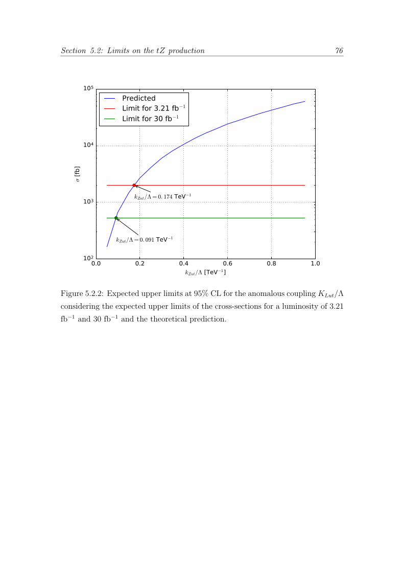
Section 5.2: Limits on the tZ production 76
0.0 0.2 0.4 0.6 0.8 1.0kZut/Λ [TeV−1]
102
103
104
105
σ [f
b]
kZut/Λ=0. 174 TeV−1
kZut/Λ=0. 091 TeV−1
PredictedLimit for 3.21 fb−1Limit for 30 fb−1
Figure 5.2.2: Expected upper limits at 95% CL for the anomalous couplingKLut/Λ
considering the expected upper limits of the cross-sections for a luminosity of 3.21
fb−1 and 30 fb−1 and the theoretical prediction.

Chapter 6
Conclusions
In the present thesis, a search for tZ production through FCNC using LHC data
collected by the ATLAS detector is presented. The data sample corresponds to
an integrated luminosity of 3.21 fb−1 recorded in 2015 by the ATLAS experiment
in proton-proton collisions at√s = 13 TeV. As a first step to the unblinding of
the data events in the signal region, the expected limits on the cross-section of the
tZ production were obtained in the absence of signal. The unblinding of the data
events in the signal region will be done as soon as the 2016 data be incorporated
and after the collaboration approval.
A dedicated data analysis, composed by different control regions for the main
backgrounds and a signal region focusing in the production of a top quark and
a Z boson via FCNC was developed. A signal region selection was implemented
considering the number of events remaining after all the selection cuts. However, a
study of discriminant variables was presented to better distinguish between signal
and background. The transverse mass of the W boson was the variable chosen to
be the discriminant variable for the signal region and a fit was performed taking
in account this added cut. The several sources of systematic uncertainties were
also evaluated in this analysis.
With the collaboration of the Humboldt University (Berlin) group, the expected
upper limits at 95% CL are set on the branching ratio for the decay of a top quark
into a Z boson and a u-quark. The LHC continues to deliver 13 TeV collision data,
77

Chapter 6: Conclusions 78
as shown in Figure 6.0.1, the new data will allow a increase in the sensitivity of this
process that may enable the discovery or, alternatively, constrain in a significantly
way the cross-section of the tZ production via FCNC.
Figure 6.0.1: Luminosity per year for the different centre-of-mass energy at the
LHC [100].
The posterior studies will consist in the conclusion of the study of systematic
uncertainties as well as the possibility of increasing the sensitivity of the analysis
considering multivariate techniques.

Bibliography
[1] S. L. Glashow, “Partial Symmetries of Weak Interactions,” Nucl. Phys.,
vol. 22, pp. 579–588, 1961.
[2] F. Abe et al., “Observation of top quark production in pp collisions,” Phys.
Rev. Lett., vol. 74, pp. 2626–2631, 1995.
[3] S. Abachi et al., “Observation of the top quark,” Phys. Rev. Lett., vol. 74,
pp. 2632–2637, 1995.
[4] S. L. Glashow, J. Iliopoulos, and L. Maiani, “Weak Interactions with Lepton-
Hadron Symmetry,” Phys. Rev., vol. D2, pp. 1285–1292, 1970.
[5] K. A. Olive et al., “Review of Particle Physics,” Chin. Phys., vol. C38,
p. 090001, 2014.
[6] H. Fritzsch, M. Gell-Mann, and H. Leutwyler, “Advantages of the color octet
gluon picture,” Physics Letters B, vol. 47, no. 4, pp. 365 – 368, 1973.
[7] Politzer, H. David, “Reliable Perturbative Results for Strong Interactions?,”
Phys. Rev. Lett., vol. 30, pp. 1346–1349, Jun 1973.
[8] D. J. Gross and F. Wilczek, “Ultraviolet behavior of non-abelian gauge the-
ories,” Phys. Rev. Lett., vol. 30, pp. 1343–1346, Jun 1973.
[9] S. L. Glashow, “Partial-symmetries of weak interactions,” Nuclear Physics,
vol. 22, no. 4, pp. 579 – 588, 1961.
79

80
[10] A. Salam, “Weak and Electromagnetic Interactions,” Conf. Proc.,
vol. C680519, pp. 367–377, 1968.
[11] Weinberg, Steven, “A Model of Leptons,” Phys. Rev. Lett., vol. 19, pp. 1264–
1266, Nov 1967.
[12] F. Englert and R. Brout, “Broken Symmetry and the Mass of Gauge Vector
Mesons,” Phys. Rev. Lett., vol. 13, pp. 321–323, 1964.
[13] P. W. Higgs, “Broken Symmetries and the Masses of Gauge Bosons,” Phys.
Rev. Lett., vol. 13, pp. 508–509, 1964.
[14] Guralnik, G. S. and Hagen, C. R. and Kibble, T. W. B., “Global Conser-
vation Laws and Massless Particles,” Phys. Rev. Lett., vol. 13, pp. 585–587,
Nov 1964.
[15] M. Bustamante, L. Cieri, and J. Ellis, “Beyond the Standard Model for Mon-
taneros,” in High-energy physics. Proceedings, 5th CERN-Latin-American
School, Recinto Quirama, Colombia, March 15-28, 2009, 2009.
[16] Y. Fukuda et al., “Evidence for oscillation of atmospheric neutrinos,” Phys.
Rev. Lett., vol. 81, pp. 1562–1567, 1998.
[17] M. Altmann et al., “Complete results for five years of GNO solar neutrino
observations,” Phys. Lett., vol. B616, pp. 174–190, 2005.
[18] K. Abe et al., “Evidence for the Appearance of Atmospheric Tau Neutrinos
in Super-Kamiokande,” Phys. Rev. Lett., vol. 110, no. 18, p. 181802, 2013.
[19] K. Eguchi et al., “First results from KamLAND: Evidence for reactor anti-
neutrino disappearance,” Phys. Rev. Lett., vol. 90, p. 021802, 2003.
[20] Bruce T. Cleveland and Timothy Daily and Raymond Davis, Jr. and James
R. Distel and Kenneth Lande and C. K. Lee and Paul S. Wildenhain and
Jack Ullman, “Measurement of the Solar Electron Neutrino Flux with the
Homestake Chlorine Detector,” The Astrophysical Journal, vol. 496, no. 1,
p. 505, 1998.

81
[21] K. Kroninger, A. B. Meyer, and P. Uwer, “Top-Quark Physics at the LHC,”
in The Large Hadron Collider: Harvest of Run 1 (T. Schorner-Sadenius, ed.),
pp. 259–300, 2015.
[22] http://inspirehep.net/record/1103034/plots. [Accessed: 28-06-2016].
[23] https://twiki.cern.ch/twiki/pub/AtlasProtected/FeynmanDiagrams.
[Accessed: 28-06-2016].
[24] https://atlas.web.cern.ch/Atlas/GROUPS/PHYSICS/
CombinedSummaryPlots/TOP/singletop_allchanvsroots/singletop_
allchanvsroots.pdf. [Accessed: 27-07-2016].
[25] “Measurement of the Inclusive and Fiducial Cross-Section of Single Top-
Quark t-Channel Events in pp Collisions at√s= 8 TeV,” Tech. Rep. ATLAS-
CONF-2014-007, CERN, Geneva, Mar 2014.
[26] “Measurement of the inclusive cross-section of single top-quark t-channel
production in pp collisions at√s = 13 TeV,” Tech. Rep. ATLAS-CONF-
2015-079, CERN, Geneva, Dec 2015.
[27] “Comprehensive measurements of t-channel single top-quark production
cross sections at√s = 7 TeV with the ATLAS detector,” Phys. Rev. D,
vol. 90, p. 112006, Dec 2014.
[28] S. Chatrchyan et al., “Measurement of the single-top-quark t-channel cross
section in pp collisions at√s = 7 TeV,” JHEP, vol. 12, p. 035, 2012.
[29] V. Khachatryan et al., “Measurement of the t-channel single-top-quark pro-
duction cross section and of the | Vtb | CKM matrix element in pp collisions
at√s= 8 TeV,” JHEP, vol. 06, p. 090, 2014.
[30] “Measurement of the inclusive cross section of single top quark production in
the t channel at√s = 13TeV,” Tech. Rep. CMS-PAS-TOP-16-003, CERN,
Geneva, 2016.

82
[31] G. Aad et al., “Evidence for the associated production of a W boson and a
top quark in ATLAS at√s = 7 TeV,” Phys. Lett., vol. B716, pp. 142–159,
2012.
[32] G. Aad et al., “Measurement of the production cross-section of a single top
quark in association with aW boson at 8 TeV with the ATLAS experiment,”
JHEP, vol. 01, p. 064, 2016.
[33] S. Chatrchyan et al., “Evidence for associated production of a single top
quark and W boson in pp collisions at√s = 7 TeV,” Phys. Rev. Lett.,
vol. 110, p. 022003, 2013.
[34] S. Chatrchyan et al., “Observation of the associated production of a single
top quark and a W boson in pp collisions at√s =8 TeV,” Phys. Rev. Lett.,
vol. 112, no. 23, p. 231802, 2014.
[35] “Combination of cross-section measurements for associated production of
a single top-quark and a W boson at√s = 8 TeV with the ATLAS and
CMS experiments,” Tech. Rep. ATLAS-CONF-2016-023, CERN, Geneva,
May 2016.
[36] “Combination of cross-section measurements of associated production of a
single top quark and a W boson at√s = 8 TeV with the ATLAS and CMS
experiments,” Tech. Rep. CMS-PAS-TOP-15-019, CERN, Geneva, 2016.
[37] “Search for s-Channel Single Top-Quark Production in pp Collisions at√s
= 7 TeV,” Tech. Rep. ATLAS-CONF-2011-118, CERN, Geneva, Aug 2011.
[38] “Evidence for single top-quark production in the s-channel in proton–proton
collisions at√s = 8 TeV with the ATLAS detector using the Matrix Element
Method,” Phys. Lett. B, vol. 756, pp. 228–246. 16 p, Nov 2015.
[39] V. Khachatryan et al., “Search for s channel single top quark production in
pp collisions at√s = 7 and 8 TeV,” 2016.

83
[40] “Fiducial t channel single top-quark cross section at 8 TeV,” Tech. Rep.
CMS-PAS-TOP-15-007, CERN, Geneva, 2015.
[41] Kidonakis, Nikolaos, “Next-to-next-to-leading-order collinear and soft gluon
corrections for t-channel single top quark production,” Phys. Rev. D, vol. 83,
p. 091503, May 2011.
[42] Kidonakis, Nikolaos, “Two-loop soft anomalous dimensions for single top
quark associated production with a W− or H−,” Phys. Rev. D, vol. 82,
p. 054018, Sep 2010.
[43] Kidonakis, Nikolaos, “Next-to-next-to-leading logarithm resummation for s-
channel single top quark production,” Phys. Rev. D, vol. 81, p. 054028, Mar
2010.
[44] P. Kant, O. Kind, T. Kintscher, T. Lohse, T. Martini, S. Molbitz, P. Rieck,
and P. Uwer, “Hathor for single top-quark production: Updated predictions
and uncertainty estimates for single top-quark production in hadronic colli-
sions,” Computer Physics Communications, vol. 191, pp. 74 – 89, 2015.
[45] R. Guedes, R. Santos, and M. Won, “Limits on strong flavor changing neutral
current top couplings at the LHC,” Phys. Rev., vol. D88, no. 11, p. 114011,
2013.
[46] P. M. Ferreira and R. Santos, “Strong flavor changing effective operator con-
tributions to single top quark production,” Phys. Rev., vol. D73, p. 054025,
2006.
[47] A. Amorim, J. P. Araque, N. F. Castro, J. Santiago, and R. Santos, “Pro-
duction of tγ, tZ and tH via Flavour Changing Neutral Currents,” PoS,
vol. TOP2015, p. 067, 2016.
[48] R. Coimbra, A. Onofre, R. Santos, and M. Won, “MEtop – a top FCNC
event generator,” J. Phys. Conf. Ser., vol. 447, p. 012031, 2013.

84
[49] C. Degrande, F. Maltoni, J. Wang, and C. Zhang, “Automatic computa-
tions at next-to-leading order in QCD for top-quark flavor-changing neutral
processes,” Phys. Rev., vol. D91, p. 034024, 2015.
[50] J. A. Aguilar-Saavedra, “Top flavor-changing neutral interactions: Theoret-
ical expectations and experimental detection,” Acta Phys. Polon., vol. B35,
pp. 2695–2710, 2004.
[51] V. M. Abazov et al., “Search for flavor changing neutral currents via quark-
gluon couplings in single top quark production using 2.3 fb−1 of pp collisions,”
Phys. Lett., vol. B693, pp. 81–87, 2010.
[52] “Search for the flavor-changing neutral-current decay t→ Zq in pp collisions
at√s=1.96TeV,” Physical Review Letters, vol. 101, 11 2008.
[53] G. Aad et al., “Search for single top-quark production via flavour-changing
neutral currents at 8 TeV with the ATLAS detector,” Eur. Phys. J., vol. C76,
no. 2, p. 55, 2016.
[54] V. Khachatryan et al., “Search for anomalous single top quark production
in association with a photon in pp collisions at√s = 8 TeV,” JHEP, vol. 04,
p. 035, 2016.
[55] G. Aad et al., “Search for flavour-changing neutral current top-quark decays
to qZ in pp collision data collected with the ATLAS detector at√s = 8
TeV,” Eur. Phys. J., vol. C76, no. 1, p. 12, 2016.
[56] “Search for Flavour Changing Neutral Currents in single top events,” Tech.
Rep. CMS-PAS-TOP-12-021, CERN, Geneva, 2013.
[57] S. Chatrchyan et al., “Search for Flavor-Changing Neutral Currents in Top-
Quark Decays tZq in pp Collisions at√s = 8TeV,” Phys. Rev. Lett., vol. 112,
no. 17, p. 171802, 2014.

85
[58] “Search for associated production of a Z boson with a single top quark and
for tZ flavour-changing interactions in pp collisions at sqrt(s) = 8 TeV,”
Tech. Rep. CMS-PAS-TOP-12-039, CERN, Geneva, 2016.
[59] https://atlas.web.cern.ch/Atlas/GROUPS/PHYSICS/
CombinedSummaryPlots/TOP/. [Accessed: 12-07-2016].
[60] Lyndon Evans and Philip Bryant, “LHC Machine,” Journal of Instrumenta-
tion, vol. 3, no. 08, p. S08001, 2008.
[61] The ATLAS Collaboration, “The ATLAS Experiment at the CERN Large
Hadron Collider,” Journal of Instrumentation, vol. 3, no. 08, p. S08003, 2008.
[62] https://cds.cern.ch/record/2119882. [Accessed: 17-06-2016].
[63] F. J. Hasert et al., “Observation of Neutrino Like Interactions Without Muon
Or Electron in the Gargamelle Neutrino Experiment,” Phys. Lett., vol. B46,
pp. 138–140, 1973.
[64] G. Arnison et al., “Experimental Observation of Isolated Large Transverse
Energy Electrons with Associated Missing Energy at s**(1/2) = 540-GeV,”
Phys. Lett., vol. B122, pp. 103–116, 1983. [,611(1983)].
[65] M. Banner et al., “Observation of Single Isolated Electrons of High Trans-
verse Momentum in Events with Missing Transverse Energy at the CERN
anti-p p Collider,” Phys. Lett., vol. B122, pp. 476–485, 1983.
[66] S. Schael et al., “Precision electroweak measurements on the Z resonance,”
Phys. Rept., vol. 427, pp. 257–454, 2006.
[67] V. Fanti et al., “A New measurement of direct CP violation in two pion
decays of the neutral kaon,” Phys. Lett., vol. B465, pp. 335–348, 1999.
[68] G. Aad et al., “Observation of a new particle in the search for the Standard
Model Higgs boson with the ATLAS detector at the LHC,” Phys. Lett.,
vol. B716, pp. 1–29, 2012.

86
[69] S. Chatrchyan et al., “Observation of a new boson at a mass of 125 GeV
with the CMS experiment at the LHC,” Phys. Lett., vol. B716, pp. 30–61,
2012.
[70] The ALICE Collaboration, “The ALICE experiment at the CERN LHC,”
Journal of Instrumentation, vol. 3, no. 08, p. S08002, 2008.
[71] The CMS Collaboration, “The CMS experiment at the CERN LHC,” Jour-
nal of Instrumentation, vol. 3, no. 08, p. S08004, 2008.
[72] The LHCb Collaboration, “The LHCb Detector at the LHC,” Journal of
Instrumentation, vol. 3, no. 08, p. S08005, 2008.
[73] https://cds.cern.ch/record/1095926. [Accessed: 17-06-2016].
[74] https://cds.cern.ch/record/1095927. [Accessed: 17-06-2016].
[75] http://cds.cern.ch/record/1095929. [Accessed: 17-06-2016].
[76] https://twiki.cern.ch/twiki/bin/view/AtlasPublic/
LuminosityPublicResultsRun2#Luminosity_summary_plots_for_AN1.
[Accessed: 07-07-2016].
[77] G. Duckeck, D. Barberis, R. Hawkings, R. Jones, N. McCubbin, G. Poulard,
D. Quarrie, T. Wenaus, and E. Obreshkov, “ATLAS computing: Technical
design report,” 2005.
[78] http://wlcg-public.web.cern.ch/tier-centres. [Accessed: 10-07-
2016].
[79] J.-L. Agram, J. Andrea, E. Conte, B. Fuks, D. Gele, and P. Lansonneur,
“Probing top anomalous couplings at the LHC with trilepton signatures in
the single top mode,” Phys. Lett., vol. B725, pp. 123–126, 2013.
[80] https://ms2.physik.hu-berlin.de/~atlas/aplusplus/htmldoc/. A++
Reference Guide.

87
[81] “2015 start-up trigger menu and initial performance assessment of the
ATLAS trigger using Run-2 data,” Tech. Rep. ATL-DAQ-PUB-2016-001,
CERN, Geneva, Mar 2016.
[82] “Performance of the ATLAS muon trigger in 2011,” Tech. Rep. ATLAS-
CONF-2012-099, CERN, Geneva, Jul 2012.
[83] “Electron efficiency measurements with the ATLAS detector using the 2015
LHC proton-proton collision data,” Jun 2016.
[84] “Muon reconstruction performance of the ATLAS detector in proton–proton
collision data at 13 TeV,” Eur. Phys. J. C, vol. 76, p. 292. 45 p, Mar 2016.
[85] M. Cacciari, G. P. Salam, and G. Soyez, “The Anti-k(t) jet clustering algo-
rithm,” JHEP, vol. 04, p. 063, 2008.
[86] M. Cacciari and G. P. Salam, “Dispelling the N3 myth for the kt jet-finder,”
Phys. Lett., vol. B641, pp. 57–61, 2006.
[87] M. Cacciari, G. P. Salam, and G. Soyez, “FastJet user manual,” Eur. Phys.
J. C, vol. 72, p. 1896. 69 p, Nov 2011.
[88] T. Barillari, E. Bergeaas Kuutmann, T. Carli, J. Erdmann, P. Giovannini,
K. J. Grahn, C. Issever, A. Jantsch, A. Kiryunin, K. Lohwasser, A. Maslen-
nikov, S. Menke, H. Oberlack, G. Pospelov, E. Rauter, P. Schacht, F. Spano,
P. Speckmayer, P. Stavina, and P. Strızenec, “Local Hadronic Calibration,”
Tech. Rep. ATL-LARG-PUB-2009-001-2. ATL-COM-LARG-2008-006. ATL-
LARG-PUB-2009-001, CERN, Geneva, Jun 2008. Due to a report-number
conflict with another document, the report-number ATL-LARG-PUB-2009-
001-2 has been assigned.
[89] “Monte Carlo Calibration and Combination of In-situ Measurements of Jet
Energy Scale, Jet Energy Resolution and Jet Mass in ATLAS,” Tech. Rep.
ATLAS-CONF-2015-037, CERN, Geneva, Aug 2015.

88
[90] “Jet Calibration and Systematic Uncertainties for Jets Reconstructed in the
ATLAS Detector at√s = 13 TeV,” Tech. Rep. ATL-PHYS-PUB-2015-015,
CERN, Geneva, Jul 2015.
[91] “Expected performance of the ATLAS b-tagging algorithms in Run-2,” Tech.
Rep. ATL-PHYS-PUB-2015-022, CERN, Geneva, Jul 2015.
[92] https://atlas.web.cern.ch/Atlas/GROUPS/PHYSICS/PUBNOTES/
ATL-PHYS-PUB-2015-022/figaux_02a.png. [Accessed: 02-08-2016].
[93] https://atlas.web.cern.ch/Atlas/GROUPS/PHYSICS/PUBNOTES/
ATL-PHYS-PUB-2015-022/figaux_02b.png. [Accessed: 02-08-2016].
[94] J. Alwall, M. Herquet, F. Maltoni, O. Mattelaer, and T. Stelzer, “MadGraph
5 : Going Beyond,” JHEP, vol. 06, p. 128, 2011.
[95] T. Sjostrand, S. Mrenna, and P. Z. Skands, “PYTHIA 6.4 Physics and Man-
ual,” JHEP, vol. 05, p. 026, 2006.
[96] Stefano Frixione and Paolo Nason and Carlo Oleari, “Matching NLO QCD
computations with parton shower simulations: the POWHEG method,”
Journal of High Energy Physics, vol. 2007, no. 11, p. 070, 2007.
[97] “Jet Calibration and Systematic Uncertainties for Jets Reconstructed in the
ATLAS Detector at√s = 13 TeV,” Tech. Rep. ATL-PHYS-PUB-2015-015,
CERN, Geneva, Jul 2015.
[98] T. Junk, “Confidence level computation for combining searches with small
statistics,” Nucl. Instrum. Meth., vol. A434, pp. 435–443, 1999.
[99] A. L. Read, “Presentation of search results: The CL(s) technique,” J. Phys.,
vol. G28, pp. 2693–2704, 2002. [,11(2002)].
[100] https://atlas.web.cern.ch/Atlas/GROUPS/DATAPREPARATION/
PublicPlots/2016/DataSummary/figs/intlumivsyear.png. [Accessed:
20-08-2016].