analysing binomial data conditional on number of … · web viewexamining possible explanatory...
TRANSCRIPT

Statistical Analysis of the SEERAD/SAC E. coli O157 Prevalence Study, 1998-2000
SEERAD FF Project BSS/028/99
Iain J. McKendrick
Biomathematics & Statistics Scotland
1

Executive Summary
Properties of Data
Samples from 952 farms are included in the analysis, with a total of 14,856 faecal samples analysed. Of these faecal samples, 1231 were positive for verocytotoxic E. coli O157. These positive samples were sourced from 207 farms. Hence, the raw figures indicate that 21.7% (19.2%, 24.5%) of groups sampled contained shedding animals, and that the animal level prevalence is 8.3% (7.3%, 9.4%). However, these figures do not allow for the effects of sampling error (which in a situation with many groups with a small number of shedders would tend to underestimate the number of groups containing shedders) and of the mixed nature of the sample (farms with no infection will, by definition, have zero prevalence, a more useful statistic is the estimate of the animal prevalence on those farms which are positive). The data are analysed using a beta-binomial model, from which it is estimated that the proportion of shedding animals is 7.9% with a 95% confidence interval of (6.5%, 9.6%). This is slightly lower than the raw estimate given earlier. This adjustment arises from the more appropriate modelling of the asymmetric prevalence distribution. It is estimated that 22.8% of finishing groups contained at least one positive shedding animal, with a 95% confidence interval of (19.6%, 26.3%). The point-estimate and confidence interval are both slightly higher than the raw estimates given earlier, since these figures incorporate an adjustment to allow for farms with low shedding rates being misclassified as negative due to sampling variability.
Analysis of Within-Farm Prevalences
These data are highly skewed, with many zero returns. This is because their true statistical distribution should be a mixture distribution, with true negative farms always generating a zero response and positive farms generating a range of responses, many of which will be zero, with variability arising from the between-farm variability and the sampling variability. Ignoring this aspect of the data gives rise to models with unacceptable residuals. The data is handled by restricting analysis to those observations with non-zero responses. Hence, the epidemiological analysis answers the question ‘given that the farm has at least one positive sample, what factors tend to be associated with higher within-farm prevalences?’
The data are analysed by fitting a series of generalised linear models to each variable in turn, developing a multivariate model (using some of the stepwise regression functions available for this class of model) containing all likely factors, and then refitting this model as a generalised linear mixed model (GLMM). Hence the ultimate model uses the most appropriate algorithm for the data. The data are consistently fitted as binomial random variables with logit link functions. Generalised linear models are consistently fitted with estimated dispersion parameters (all of which are clearly greater than one), while the GLMMs are fitted with Farm as a random effect and fixed dispersion (since farm is the basic sampling unit). Other possible random effects are insignificant.
Within the univariate analysis, examining structural variables, animal health division and sampling month are found to be highly significant. Examining possible
2

explanatory variables, we find that housing status (housed or unhoused) has an extremely significant effect on the prevalences (housed animals have a much higher prevalence than unhoused animals).
Factor/Variable Effect CommentDivision Highland area has a higher
prevalence, South-West has a low prevalence.
Effect even stronger in ultimate multivariate model.
Sampling Month Lower in summer months. Effect disappears in ultimate multivariate model. Effect explained by differential housing in different months.
Season/ Seas_List Summer and Autumn show lower prevalences.
Effect better explained by examining results on a month by month basis. Effect disappears in multivariate model.
Housed Housed animals have a much higher prevalence. Highly significant.
This is the key finding of the study. All other parts of the analysis depend on the correct modelling of the ‘Housed’ effect.
Recent Move A recent move is associated with lower prevalences.
This effect becomes even more clear when explored in conjunction with ‘Housed’.
Recent Change in Feed Recent change in feed associated with lower prevalences.
This effect becomes even more clear when explored in conjunction with ‘Housed’.
Silage_Home Silage production on the farm is associated with lower prevalence in housed animals.
Effect explained more fully in multivariate analysis.
Silage_Slurry Silage production on the farm with the spreading of slurry is associated with lower prevalence in housed animals.
Effect explained more fully in multivariate analysis.
N_Pigs Higher number of pigs is associated with lower prevalence.
Model result depends on 8 points with high leverage. Suspicious that categorical variable derived from this variable (Pigs) is not significant. Effect found not to be significant in final multivariate model. Probably spurious.
3

N_Deer Higher number of deer is associated with higher prevalence.
Model result depends on 1 point with high leverage. No basis for drawing any wider conclusions from this result. Probably spurious.
Water Natural water supplies associated with significantly lower prevalences than main supply.
Natural water supplies associated with unhoused animals. Even so, natural water supply is associated with lower prevalence.
Housing, Supplementary Feed, Forage, Silage, Concentrate, Grass_Manure, Grass_Slurry, Grass_Sewage, Grass_Geece, Grass_Gulls
All of these factors, although apparently significant in the univariate analysis, are confounded with Housed.
No information above that gained from ‘Housed’
Fitting a multi-factor model, particularly exploring the interactions between the Housed variable and the other possible variables, we find that the following factors are of interest:
Factor/Variable
Effect Log Odds Ratio
se p-value
Housed Housed animals have higher prevalences.
1.319 0.33 <0.001
FCattle Farms with >100 finishing cattle have significantly lower prevalences than those with <100.
-0.702 0.23 0.004
Housed/’Recent Changes in Housing or Diet’ interactions
Farms with Housed Animals and recent changes have higher prevalences than farms with unhoused animals. This effect is not formally significant.Farms with Housed Animals and no recent changes have higher prevalences than farms with Housed Animals and recent changes.
0.480
0.891
0.43
0.33
0.26
0.007
Water sourced from natural supply
Farms with animals at pasture have lower prevalences if the water is from a natural source.
-0.708 0.35 0.04
4

Slurry spread on Farm
Farms with housed animals which spread slurry on their silage fields have a lower prevalence than farms with housed animals which do not.
-0.5529 0.29 0.07
Animal Health Division
Scotland divided into three regions: Highlands; Central, Islands, North-East and South-East; and South West.Highlands exhibits a significantly higher prevalence than the portmanteau region.The South West exhibits a significantly lower prevalence than the portmanteau region.
0.969
-0.600
0.42
0.28
0.02
0.03
Sampling Month No significant effects identified. All variability explained by explanatory variables above, especially Housed.
Various Various 0.23
Sampling Year No significant effects identified.
Various Various 0.61
Hence, various explanatory factors and variables have been identified as being associated with the within-farm prevalence of E. coli O157 shedding in finishing cattle on positive farms. No statistically significant management system variability was observed in the analysis of the basic data, and nothing further became apparent following the fitting of the multi-factor model. Similarly, there was no evidence of any long-term trend in prevalences over the lifetime of the study, and this conclusion remained unaffected by the fitting of the multi-factor model. By contrast, the basic data showed evidence of variability between different Animal Health Divisions, and this effect remained in the multi-factor model, unexplained by any of the proposed explanatory factors. The basic data showed highly significant evidence of cyclicity by month. When included in a model with the full multi-factor model, the month effect was found to be insignificant, being fully explained by other explanatory factors. Hence it can be concluded that although the within-farm prevalences do vary with month, this is explained by the proposed explanatory factors. By contrast, the geographical variability in the data appears to be genuine, and is best examined after the extraneous effects of the other explanatory factors have been allowed for in the model.
Analysis of Between-Farm Prevalences
The detailed data collected in the study can be converted into binary (or Bernoulli) data, where the farm is recorded as a positive if at least one of the samples collected from that farm is positive, and negative if all samples are negative. The binary data can then be analysed in terms of the probability of observing a positive farm on different types of farm. These data present fewer difficulties in analysis than the within-farm prevalence data: since only positives and negatives are recorded, it is
5

impossible for a generalised linear model to provide a poor fit in terms of the distribution of residuals, since the data does not contain enough structure for any lack of fit to occur. Accordingly, all the models in this section are fitted with dispersion parameter set equal to one, since it is impossible to estimate any such over-dispersion from the data. Many of the diagnostics which are available in terms of the fit of the model for Binomial data are not useful for Bernoulli data. It is appropriate to examine the data in this format for two reasons: firstly, since zero prevalence farms have been excluded from the within-farm analysis for technical statistical reasons, it is desirable to investigate the factors which are associated with farms being negative, since otherwise these data will have never have been analysed. Secondly, there is no reason to believe that the factors which promote high within-herd prevalences on farms which are positive will be the same as the factors which either promote the infection of farms with E. coli O157 or which encourage the maintenance of infection once introduced. Obviously, a factor which is associated with high within-herd prevalence will have potential to also be associated with a high probability of herd infection, however, it will be interesting to identify where different factors may come into play in the two models.
The data are analysed by fitting a series of generalised linear models to each variable in turn, developing a multivariate model (using some of the stepwise regression functions available for this class of model) containing all likely factors, and then refitting this model as a generalised linear mixed model (GLMM). Hence the ultimate model uses the most appropriate algorithm for the data. The data are consistently fitted as Bernoulli random variables with logit link functions. Generalised linear models are consistently fitted with dispersion parameters fixed equal to one, while the GLMMs are fitted with Farm as a random effect and a fixed dispersion (since farm is the basic sampling unit). Other possible random effects are found to be insignificant.
Within the univariate analysis, examining structural variables, none are found to be highly significant. There is some weak evidence of an effect due to Sampling Year, but this effects are not significant at the 5% level. Examining possible explanatory variables, by contrast to the within-herd model, we find that Housing status has a negligible effect on the probability of a farm being identified as positive. The following factors were found to be of interest in the univariate analysis:
Factor/Variable Effect CommentDivision No formally statistically
significant effects. Highland division has a particularly low prevalence.
No trend apparent, although it is interesting that Highlands are so low, when the within-herd prevalence was high. Effects utterly disappear in the multifactor model.
Sampling Month No statistically significant evidence of any effects (p=0.26). Prevalences from December to February show signs of being lower.
In the within-farm model, January-April tended to show higher prevalences, associated with Housing effects. This aspect of the dataset requires careful interpretation, since data
6

from early 2000 is included in the January to April estimates, and not in the other months. There is some evidence that the data from 2000 exhibits a lower prevalence. Hence this variable is analysed along with Sampling Year. However, even when Year and Sample Month are fitted in the same model, there is only weak evidence of any effect due to Sampling Month. However, the effects which are apparent in the univariate analysis can be shown be significant within the multifactor analysis.
Sampling Year A small drop in 1999 and a large drop in 2000. The result is close to statistical significance (p=0.06).
Due to a lack of balance in the dataset, this result is derived from a model fitted with Sampling Month. There is compelling evidence of a drop in prevalence by year 2000, less so for year 1999. Similar results are seen in the multifactor model, where the trend is highly significant.
Number of Finishing Cattle Higher numbers of finishing cattle were associated with a high risk of the farm being positive. P-value suppressed as arising from a poorly fitting model.
Each of the eight significant cattle number factors and variables gives the same result: more animals equates to a higher risk of the farm being positive. Some are rejected as presenting a poorly fitting model: others because another factor is found to be more informative. This variate was overly sensitive to a small number of farms with high numbers of finishing cattle.
Categorised Number of Categorising the numbers One of the most
7

Finishing Cattle of animals into 4 classes, groups containing 1-49 animals were less likely to be identified as positive than larger groups, while groups of >200 animals had even higher prevalences still. Effects are highly statistically significant (p<0.001).
informative factors in this sub-grouping. Carried forward for further investigation in the multi-factor model.
Number of Groups of Cattle Higher numbers of groups of cattle were associated with a higher risk of the farm being positive. p-value suppressed as arising from a poorly fitting model.
This variate was overly sensitive to a small number of farms with high numbers of groups of cattle.
Categorised Number of Groups of Cattle
Higher numbers of groups of cattle were associated with a higher risk of the farm being positive. (p=0.08). Fit still fairly poor.
Factor relatively insignificant. Lacked information relative to other terms in the sub-grouping.
Number of Cattle in Sampling Group
Higher numbers of animals in the sampling group were associated with a higher risk of the farm being positive. p-value suppressed as arising from a poorly fitting model.
This variate was overly sensitive to a small number of farms with high numbers of groups of cattle.
Categorised Number of Cattle in Sampling Group
Higher numbers of animals in the sampling group were associated with a higher risk of the farm being positive (p<0.001).
Carried forward for further investigation in the multi-factor model.
Number of Cattle Higher numbers of cattle were associated with a higher risk of the farm being positive. p-value suppressed as arising from a poorly fitting model.
This variate was overly sensitive to a small number of farms with high numbers of cattle.
Categorised Number of Cattle Higher numbers of cattle were associated with a higher risk of the farm being positive. (p=0.002).
Carried forward for further investigation in the multi-factor model. Lacks significance when fitted with other factors.
Source of Cattle Farms which never buy in animals have a
Lacks significance when fitted with other factors in
8

significantly lower (p=0.03) risk of being positive than those which always or sometimes buy in animals.
the multivariate model. When number of finishing cattle or number of sampling groups are included in the model, it can be seen that source of cattle lacks explanatory power.
Breed Farms with B_D_DB class animals have a higher prevalence than others (p=0.018).
An extremely small level, with a correspondingly high leverage, it is not surprising that it is found to lack significance when fitted with other factors.
Beef Cattle on Dairy Farm Farms which are described as having a dairy system with beef cattle have a statistically significantly higher risk of being positive than other farms (p=0.017).
Risk group identified from analysis of interaction of two more broadly defined factors. Possible risk of over-trawling the data.
Spreading of Slurry on Pasture
Farms with unhoused animals which spread slurry on the pasture have a higher risk of being positive than those which do not, or those which have housed animals. (p=0.003).
Spreading of Manure on Pasture
Farms with unhoused animals which spread manure on the pasture have a lower risk of being positive than those which do not, or those which have housed animals. (p=0.037).
Number of Goats High number of goats is associated with a higher risk of farm being positive. p-value suppressed as arising from a poorly fitting model.
This variate was overly sensitive to two farms with higher numbers of goats.
Presence of Pigs on Farm The presence of pigs on a farm is associated with a higher risk of the farm being classed as positive (p=0.01).
Lab Operator The identity of the lab operator who carried out
This effect was found to be spurious, arising from the
9

the assaying of the samples was found to be a significant effect (p=0.039).
unbalanced nature of the data with respect to this factor. Different operators carried out work at different times, on samples with different mean prevalences.
Max Age of Animals in Group
A higher maximum age is associated with a lower prevalence (p=0.31).
This variate is included for completeness, since it is found to be relevant in the multi-factor model, although, as can be seen, it lacks any apparent explanatory power in isolation.
Fitting a multi-factor model, we find that the following factors and variates are of interest:
Factor/Variable
Effect Log Odds Ratio
se p-value
Sampling Year Allowing for the explanatory factors, farms sampled in year 1999 are at lower risk of being positive than those sampled in 1998.
Allowing for the explanatory factors, farms sampled in year 2000 are at lower risk of being positive than those sampled in 1999.
Allowing for the explanatory factors, farms sampled in year 2000 are at lower risk of being positive than those sampled in 1998.
-0.425
-0.371
-0.795
0.21
0.26
0.31
0.04
0.15
0.01
Sampling Month
A broad cyclical effect, with prevalence effects peaking in Summer and troughing in Winter. Anomalous changes in prevalences observed in a number of months, such as June, April and November.
Various Various 0.02
10

Categorised Number of Animals in Sampling Group.
Farms with 12-28 animals are at a higher risk of being positive than those with <12 animals.
Farms with >28 animals are at a higher risk of being positive than those with 12-28 animals.
0.687
0.462
0.23
0.19
0.003
0.03
Categorised Number of Finishing Cattle.
Farms with 50-199 animals are at a higher risk of being positive than those with 1-49 animals.
Farms with 200+ animals are at a higher risk of being positive than those with 50-199 animals.
0.367
0.614
0.19
0.30
0.05
0.04
Spreading of Slurry on Pasture
Considering only farms with animals at pasture, those which spread slurry are at a higher risk than those which do not.
1.205 0.32 <0.001
Spreading of Manure on Pasture
Considering only farms with animals at pasture, those which spread manure are at a lower risk than those which do not.
-1.155 0.36 0.001
Dairy Farms with Beef Cattle
Dairy farms with beef cattle are at a higher risk of being positive than other farms.
1.965 0.64 0.002
Presence of pigs on farm.
Farms with pigs are at a higher risk of being positive than those without pigs.
0.892 0.35 0.01
Maximum age of cattle in sampling group.
Higher maximum age is associated with a lower risk of the farm being positive.
-0.031 0.015 0.04
Of these, it should be pointed out that the factor ‘Categorised Number of Animals in Sampling Group’ is correlated with the number of animals in the sampling group and hence with the number of samples collected from the group. Hence it might be thought likely that a positive relationship might be generated through the higher detection probability arising from a larger sample. Consideration of the data suggests that this is unlikely, but even if the result is discounted on this basis, the inclusion of FCattle in the model even in the presence of the sampling group factor indicates that the size of enterprise is a highly significant risk factor.
11

Hence, various explanatory factors and variables have been identified as being associated with the farm prevalence of E. coli O157 shedding in finishing cattle. No statistically significant geographical or management system variability was observed in the analysis of the basic data, and nothing further became apparent following the fitting of the multi-factor model. By contrast, the basic data showed evidence of a long-term trend towards lower prevalences over the lifetime of the study, and this trend remained in the multi-factor model, unexplained by any of the proposed explanatory factors. The basic data showed no significant evidence of any cyclicity by month or season, although various peculiarities were observable in the analysis. When included in a model with the full multi-factor model, the month effect is found to be significant. It is important to stress that this significance is associated with the same peculiarities observed in the univariate model: the effect is not an artefact of a poorly fitting model. Hence it can be concluded that the farm level prevalences do vary with month, in a fashion which is not explained by the proposed explanatory factors.
12

Properties of Data
Samples from 952 farms are included in the analysis, with a total of 14,856 faecal samples analysed. Of these faecal samples, 1231 were positive for verocytotoxic E. coli O157. These positive samples were sourced from 207 farms. Hence, the raw figures indicate that 21.7% (19.2%, 24.5%) of groups sampled contained shedding animals.
126 "Modelling of binomial proportions. (e.g. by logits)." 127 MODEL [DISTRIBUTION=binomial; LINK=logit; DISPERSION=1] VFarmPos; NBINOMIAL=1 128 FIT [PRINT=model,summary,estimates; CONSTANT=estimate; FPROB=yes; TPROB=yes; FACT=9]\ 129
129............................................................................. ***** Regression Analysis ***** Response variate: VFarmPos Binomial totals: 1 Distribution: Binomial Link function: Logit Fitted terms: Constant *** Summary of analysis *** mean deviance approx d.f. deviance deviance ratio chi prRegression 0 0.0 *Residual 951 997.0 1.048Total 951 997.0 1.048* MESSAGE: ratios are based on dispersion parameter with value 1 Dispersion parameter is fixed at 1.00 *** Estimates of parameters *** antilog of estimate s.e. t(*) t pr. estimateConstant -1.2807 0.0786 -16.30 <.001 0.2779* MESSAGE: s.e.s are based on dispersion parameter with value 1
Analysis of the animal level prevalence is complicated by the need to fit a dispersion parameter and the (frankly) appalling fit of the model, giving a mean and confidence interval of 8.3% (7.3%, 9.4%).
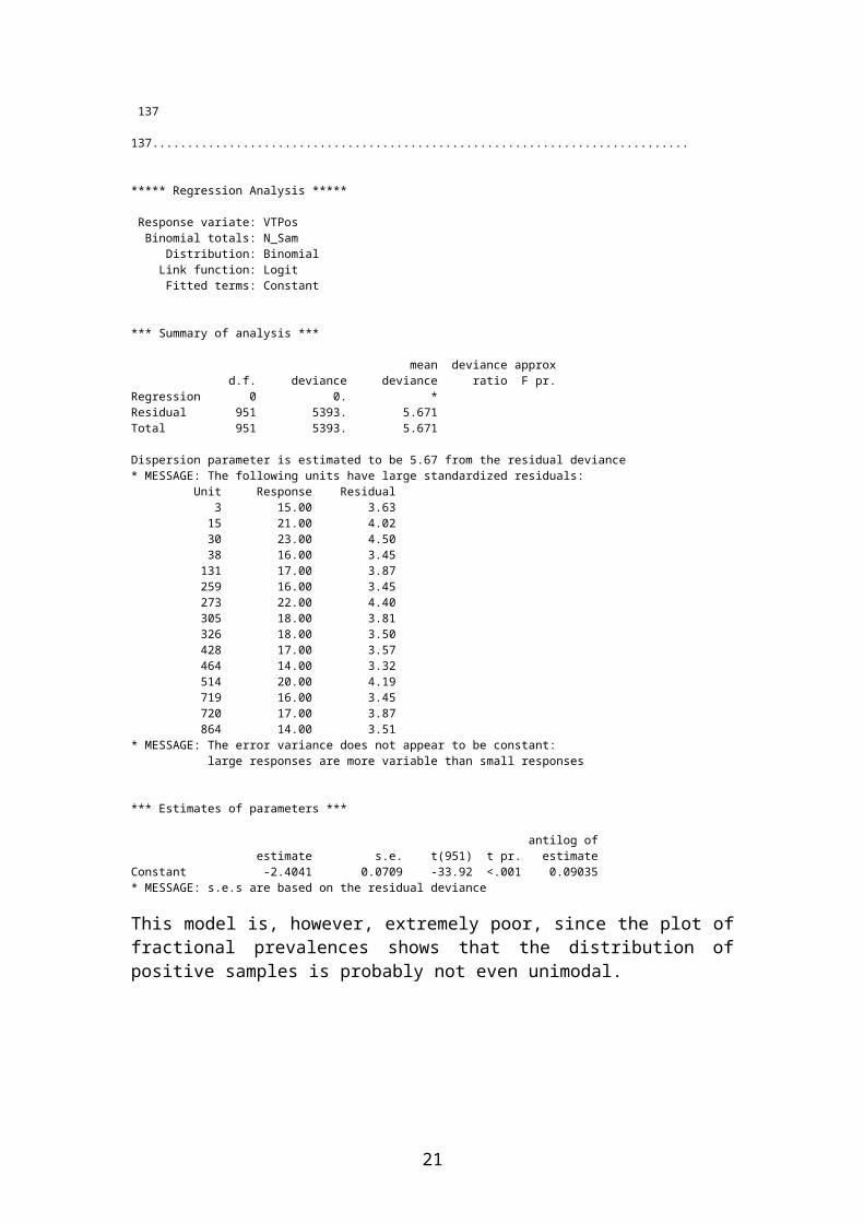
134 "Modelling of binomial proportions. (e.g. by logits)." 135 MODEL [DISTRIBUTION=binomial; LINK=logit; DISPERSION=*] VTPos; NBINOMIAL=N_Sam 136 FIT [PRINT=model,summary,estimates; CONSTANT=estimate; FPROB=yes; TPROB=yes; FACT=9]\ 137 137............................................................................. ***** Regression Analysis ***** Response variate: VTPos Binomial totals: N_Sam Distribution: Binomial Link function: Logit Fitted terms: Constant *** Summary of analysis *** mean deviance approx
13

d.f. deviance deviance ratio F pr.Regression 0 0. *Residual 951 5393. 5.671Total 951 5393. 5.671 Dispersion parameter is estimated to be 5.67 from the residual deviance* MESSAGE: The following units have large standardized residuals: Unit Response Residual 3 15.00 3.63 15 21.00 4.02 30 23.00 4.50 38 16.00 3.45 131 17.00 3.87 259 16.00 3.45 273 22.00 4.40 305 18.00 3.81 326 18.00 3.50 428 17.00 3.57 464 14.00 3.32 514 20.00 4.19 719 16.00 3.45 720 17.00 3.87 864 14.00 3.51* MESSAGE: The error variance does not appear to be constant: large responses are more variable than small responses *** Estimates of parameters *** antilog of estimate s.e. t(951) t pr. estimateConstant -2.4041 0.0709 -33.92 <.001 0.09035* MESSAGE: s.e.s are based on the residual deviance
This model is, however, extremely poor, since the plot of fractional prevalences shows that the distribution of positive samples is probably not even unimodal.
Histogram of Fractional Prevalences.
However, these figures do not allow for the effects of sampling error (which in a situation with many groups with a small number of shedders would tend to underestimate the number of groups containing shedders) and of the mixed nature of
14

the sample (farms with no infection will, by definition, have zero prevalence, a more useful statistic is the estimate of the animal prevalence on those farms which are positive).
In order to deal with these issues, a more complex model for the within-herd prevalence distribution is proposed. The data are treated as being the outcome of a mixture distribution, where a proportion pneg of the population are defined as negative farms and will always return a zero number of positive samples. Among the positive population, the between farm variability is modelled as a beta distribution, taking parameters a and b, while the sampling distribution of the faecal pat sampling process is taken to be binomial. A small number of farms were sampled using rectal samples. The sampling distribution of this process is taken to be hypergeometric. No positive samples were collected from rectally sampled groups. Hence, where N is the number of animal in the group, n is the number of samples collected, and x is the observed number of positives, the distribution of x is taken to be:
Hence, although two different sampling distributions are involved, they are based on the same underlying parameters and can be incorporated into the same likelihood. The log-likelihood is maximised with respect to a, b and pneg.
Parameter Valuepneg 3.98E-31a 0.0687b 0.8013
The beta function to model the between farm variability in positive groups has a bi-modal shape, reflecting the long tail towards high proportional prevalences. The population contains a large proportion of groups with low prevalences, which are likely to give rise to observations of zero positives. This means that the estimate for pneg and for a and b are highly negatively correlated.
15

0
1
2
3
4
5
6
0 0.2 0.4 0.6 0.8 1
Proportion Shedding
Between-farm variability as summarised by the beta function.
The fit of the model was tested against the faecal pat-sampled observations. These data were categorised by sample size, and expected values for each response given the model were calculated. Many of these expectations were extremely small, so the expectations and observations were grouped into larger combinations with expectations of at least 5. 55 variables were used to calculate a goodness of fit statistic. However, the expectations also incorporated 26 constraints, conditioning on the number of farms associated with each of the sample sizes. Hence there were 29 degrees of freedom associated with the test statistic. The fit to the data is found to be adequate, with a chi-squared goodness-of-fit test generating a test statistic which has a p-value of 0.16. The mean animal-level prevalence on positive farms was
estimated by the mean of the beta distribution, and the mean farm level
prevalence was estimated using a more complex procedure which took account of the distribution of numbers of finishing cattle in the groups sampled in the study.
This distribution has a highly skewed distribution, as shown below:
16

Histogram of Number of Cattle in Sampling Groups.However, when the number of cattle are log-transformed, the distribution looks much more symmetric:
Histogram of the Log of Number of Cattle in Sampling Groups.
The distribution of number of cattle in the sampling groups is modelled as a log-normal distribution, with parameters as shown in the table below:
Parameter Valuemu 2.843549
sigma 0.708497
17

Assuming no relationship between size of group and the variability in prevalence summarised in the beta distribution, the beta-binomial model was used to estimate the fraction of of groups which contained at least one shedding animal (the parameters already estimated give enough information to do this).
Confidence intervals for the prevalences were generated by exploring the nature of the profile log-likelihood in the vicinity of the maximum, and using the chi-squared approximation to the log-likelihood ratio to define a 95% confidence region for a, b and pneg. Because of the strong negative correlation between pneg and a and b, pneg was set equal to the maximum likelihood estimate. Marginal confidence intervals for the mean prevalences were then generated from the profile log-likelihood by identifying the maximum and minimum values of the prevalences on the boundary of the confidence region specified by the chi-squared approximation to the profile log-likelihood ratio. Two variables were assumed unfixed, so the confidence interval was based on two available degrees of freedom. The results are summarised in the following table:
18

Point Estimate 95% Confidence IntervalGroup-Level
Prevalence22.8% (19.6%, 26.3%)
Overall Animal-Level Prevalence
7.9% (6.5%, 9.6%)
Just under one quarter of the groups of finishing cattle contained at least one shedding animal. The point-estimate and confidence interval are both slightly higher than the raw estimates given earlier, since these figures incorporate an adjustment to allow for farms with low shedding rates being misclassified as negative due to sampling variability. These figures imply that this misclassification occurred in just over 1% of farms sampled, and hence, that from the population of positive groups sampled, just under 5% (4.7%) were misclassified.
The overall proportion of animals estimated to be shedding is 7.9%. This is slightly lower than the raw estimate given earlier. This adjustment arises from the more appropriate modelling of the asymmetric prevalence distribution. The confidence interval, (6.5%, 9.6%), is also slightly wider, for the same reason.
It is interesting to attempt to estimate the proportion of animals shedding in positive groups. The difficult with this estimate is that because many groups may contain only a small number of shedders, and it is difficult to distinguish such positive groups (which should contribute to the estimate) from negative groups (which should not). Estimates of this proportion are highly sensitive to the estimated value of pneg and hence it is inappropriate to utilise the profile likelihood approach used to estimate the earlier confidence intervals. Confidence intervals for the mean prevalences were generated from the log-likelihood by identifying the maximum values of the prevalence on the boundary of the confidence region specified by the chi-squared approximation to the log-likelihood ratio. Three variables were varied, so the upper limit of the confidence interval was based on three available degrees of freedom. The lower bounds of the confidence interval for the within-infected groups prevalence must occur where pneg is negligible, and when this is the case, the likelihood is degenerate, with only two effective degrees of freedom. Therefore, the lower bound of the confidence interval was taken to be equal to that calculated for the overall prevalence of infected animals above, since this corresponded to a case with pneg small and two degrees of freedom. The results are summarised in the following table:
Point Estimate 95% Confidence IntervalAnimal-Level Prevalence in
Positive Groups
7.9% (6.5%, 21.0%)
The mean estimate of the shedding prevalence remains the same, at 7.9%, but the confidence intervals is much wider, reflecting this uncertainly over the status of many of the farms reported as negative. It is interesting to note that these data are consistent with, on average, as many as 1 in 5 animals in positive groups shedding.
19

Analysing binomial data conditional on number of Vtpositives being greater than zero.
Descriptive variables (Division, Sam_Month, Manage_O)
5656 MODEL [DISTRIBUTION=binomial; LINK=logit; DISPERSION=*] VTPos; NBINOMIAL=N_Sam5657 FIT [PRINT=model,summary,estimates; CONSTANT=estimate; FPROB=yes; TPROB=yes; FACT=9]\5658 Manage_O * MESSAGE: Term Manage_O cannot be fully included in the model because 1 parameter is aliased with terms already in the model (Manage_O Mixed) = 0 ***** Regression Analysis ***** Response variate: VTPos Binomial totals: N_Sam Distribution: Binomial Link function: Logit Fitted terms: Constant, Manage_O *** Summary of analysis *** mean deviance approx d.f. deviance deviance ratio F pr.Regression 2 0. 0.160 0.02 0.979Residual 204 1528. 7.489Total 206 1528. 7.418 Dispersion parameter is estimated to be 7.49 from the residual deviance* MESSAGE: The error variance does not appear to be constant: large responses are more variable than small responses* MESSAGE: The following units have high leverage: Unit Response Leverage 620 5.00 0.048 637 4.00 0.044 681 4.00 0.046 *** Estimates of parameters *** antilog of estimate s.e. t(204) t pr. estimateConstant -0.701 0.250 -2.81 0.005 0.4958Manage_O Beef 0.054 0.277 0.20 0.846 1.056Manage_O Other 0.060 0.324 0.18 0.854 1.061Manage_O Mixed 0 * * * 1.000* MESSAGE: s.e.s are based on the residual deviance Parameters for factors are differences compared with the reference level: Factor Reference level Manage_O Dairy
Manage_O shows no significant effects. By contrast, consider Division.
5659 MODEL [DISTRIBUTION=binomial; LINK=logit; DISPERSION=*] VTPos; NBINOMIAL=N_Sam5660 FIT [PRINT=model,summary,estimates; CONSTANT=estimate; FPROB=yes; TPROB=yes; FACT=9]\5661 Division ***** Regression Analysis ***** Response variate: VTPos Binomial totals: N_Sam Distribution: Binomial Link function: Logit
20
Fitted terms: Constant, Division *** Summary of analysis *** mean deviance approx d.f. deviance deviance ratio F pr.Regression 5 90. 18.017 2.52 0.031Residual 201 1438. 7.154Total 206 1528. 7.418 Dispersion parameter is estimated to be 7.15 from the residual deviance* MESSAGE: The following units have high leverage: Unit Response Leverage 15 21.00 0.092 51 3.00 0.092 139 9.00 0.088 143 1.00 0.105 566 15.00 0.092 584 10.00 0.104 637 4.00 0.101 *** Estimates of parameters *** antilog of estimate s.e. t(201) t pr. estimateConstant -0.653 0.202 -3.23 0.001 0.5205Division Highland 0.725 0.395 1.84 0.068 2.065Division Islands -0.326 0.439 -0.74 0.458 0.7218Division North East 0.096 0.269 0.36 0.722 1.100Division South East 0.243 0.303 0.80 0.424 1.275Division South West -0.531 0.305 -1.74 0.083 0.5881* MESSAGE: s.e.s are based on the residual deviance Parameters for factors are differences compared with the reference level: Factor Reference level Division Central
The prevalence in the Highlands is significantly higher than that in Central, while those in the Islands and the South West show some evidence of being lower.
0
0.1
0.2
0.3
0.4
0.5
0.6
0.7
0.8
Central Highlands Islands NE SE SW
21

Plot of prevalences by animal health division (univariate analysis), with 95% confidence intervals.
The estimated prevalences on positive farms in different divisions are as follows:
Central 34%Highlands 52%Islands 27%NE 36%SE 40%SW 23%
Hence there is evidence that the South West and Islands are low, Central, NE and SE are moderate and Highlands is high in terms of prevalence.
Examining Sampling Month,
***** Regression Analysis ***** Response variate: VTPos Binomial totals: N_Sam Distribution: Binomial Link function: Logit Fitted terms: Constant, Sam_Mon *** Summary of analysis *** mean deviance approx d.f. deviance deviance ratio F pr.Regression 11 177. 16.104 2.32 0.011Residual 195 1351. 6.928Total 206 1528. 7.418 Dispersion parameter is estimated to be 6.93 from the residual deviance* MESSAGE: The error variance does not appear to be constant: intermediate responses are more variable than small or largeresponses* MESSAGE: The following units have high leverage: Unit Response Leverage 308 16.00 0.176 326 18.00 0.164 333 14.00 0.172 *** Estimates of parameters *** antilog of estimate s.e. t(195) t pr. estimateConstant 0.301 0.460 0.65 0.514 1.351Sam_Mon Feb -1.037 0.602 -1.72 0.086 0.3545Sam_Mon Mar -0.570 0.525 -1.09 0.279 0.5656Sam_Mon Apr -0.878 0.579 -1.52 0.131 0.4155Sam_Mon May -0.535 0.517 -1.04 0.301 0.5854Sam_Mon Jun -1.458 0.591 -2.47 0.014 0.2327Sam_Mon Jul -1.407 0.569 -2.47 0.014 0.2448Sam_Mon Aug -1.008 0.556 -1.81 0.071 0.3650Sam_Mon Sep -1.695 0.594 -2.85 0.005 0.1836Sam_Mon Oct -1.730 0.581 -2.98 0.003 0.1772Sam_Mon Nov -0.653 0.540 -1.21 0.228 0.5207Sam_Mon Dec -0.542 0.661 -0.82 0.413 0.5816* MESSAGE: s.e.s are based on the residual deviance Parameters for factors are differences compared with the reference level: Factor Reference level Sam_Mon Jan
22

5745 RKEEP ; RESIDUALS=Resids; FITTEDVALUES=Fits;ESTIMATES=Para;VCOVAR=Var
Examining the associated confidence intervals:
0%
10%
20%
30%
40%
50%
60%
70%
80%
90%
Janu
ary
Febru
ary
March
April
MayJu
ne July
Augus
t
Septem
ber
Octobe
r
Novembe
r
Decembe
r
Plot of prevalences by sampling month, with 95% confidence intervals.
The estimated prevalences on positive farms in different sampling months are as follows:
23

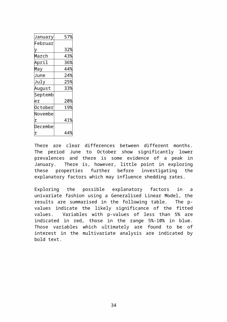
January 57%February 32%March 43%April 36%May 44%June 24%July 25%August 33%September 20%October 19%November 41%December 44%
There are clear differences between different months. The period June to October show significantly lower prevalences and there is some evidence of a peak in January. There is, however, little point in exploring these properties further before investigating the explanatory factors which may influence shedding rates.
Exploring the possible explanatory factors in a univariate fashion using a Generalised Linear Model, the results are summarised in the following table. The p-values indicate the likely significance of the fitted values. Variables with p-values of less than 5% are indicated in red, those in the range 5%-10% in blue. Those variables which ultimately are found to be of interest in the multivariate analysis are indicated by bold text.
24

Factor/Variable p-value CommentsManage_C 0.88 ‘Beef’ and ‘Others' higher than 'Dairy'Manage_O 0.98 ‘Beef’ and ‘Others' higher than 'Dairy'Division 0.03 ‘Highland’ higher than others.Sam_Month 0.01 Lower in summer monthsSample No variability in explanatory variableSam_Year 0.50 No obvious patternSeason 0.006 Summer and Autumn lower than Winter and SpringSeasList 0.04 Both Summer and Autumn lower than Winter and Spring
Sampler 0.85 ‘Fiona' is higher than 'Helen'
N_F_Cattle 0.177Higher numbers of finishing cattle associated with lower prevalence, probably better analysed as a factor, below
FCattle 0.301 No consistent pattern
N_Groups 0.35Probably better analysed as a factor, below: More groups associated with lower prevalence.
GroupsCat 0.93 No consistent pattern
N_Sam_Gr 0.22More animals in sampling group associated with lower prevalences
Min_Age 0.44 Higher minimum age associated with lower prevalenceMax_Age 0.25 Higher maximum age associated with lower prevalenceSource 0.17 ‘Buy in' and ‘Both’ lower than 'Breeding only'NewSource 0.19 ‘Open' lower than 'Closed'Breed 0.54 ‘DairyBeef' less than 'Beef', but not significant Housed <0.001 Housed animals have much higher prevalencesHousing <0.001 Housing confounded with Housed. Otherwise nothing. NoChange 0.59 1' higher than '0' (not sure of interpretation)TDHouse 0.45 Longer time associated with higher prevalencesRec_Move 0.002 A recent move is associated with lower prevalences
RecMove2 0.33Most recent move class 1 (<1 week) is lower than classes 2 and 3 (>1 week)
SupFeed <0.001 SupFeed confounded with Housed. Otherwise nothing.RecDFeed 0.007 Recent change in feed associated with lower prevalenceForage 0.007 Forage confounded with Housed.Silage 0.007 Silage confounded with Housed. Otherwise nothing.Concentrate 0.013 Concentrate confounded with Housed.
Sil_Home 0.029 ‘Yes' is lower than 'No'. Silage_Home confounded with Housed.
Sil_Manure 0.19‘Yes' is lower than 'No'. Silage_Manure confounded with Housed.
Sil_Slurry 0.108‘Yes' is lower than 'No'. Silage_Slurry confounded with Housed.
Sil_Sewage 0.44‘Yes' is lower than 'No'. Silage_Sewage confounded with Housed.
Sil_Geece 0.40‘Yes' is higher than 'No'. Silage_Geece confounded with Housed.
Sil_Gulls 0.37‘Yes' is higher than 'No'. Silage_Gulls confounded with Housed.
Hay 0.79 ‘Yes' is lower than 'No'Hay_Manure 0.58 ‘Yes' is lower than 'No'Hay_Slurry 0.69 ‘Yes' is lower than 'No'Hay_Sewage No data points in class with Sewage on hay fields.
25

Hay_Geese No data points in class with Geese on hay fields.Hay_Gulls 0.45 Gulls present associated with lower prevalence
Grass_Manure <0.001Grass_Manure confounded with Housed. Otherwise ‘Yes' is lower than 'No', but not significant.
Grass_Slurry <0.001Grass_Slurry confounded with Housed. Otherwise ‘Yes' is lower than 'No', but not significant.
Grass_Sewage <0.001Grass_Sewage confounded with Housed. Otherwise nothing.
Grass_Geece <0.001Grass_Geece confounded with Housed. Otherwise ‘Yes' is lower than 'No'
Grass_Gulls <0.001Grass_Gulls confounded with Housed. Otherwise ‘Yes' is lower than 'No'
N_Cattle 0.15 More cattle associated with lower prevalenceCattle 0.55 No clear pattern.
N_Sheep 0.37Large numbers of sheep are protective, but better analysed using a factor, below.
Sheep 0.67 (Sheep absent or present) 'With' is lower than 'Without'N_Goats 0.21 More goats associated with higher prevalenceGoats 0.46 (Goats absent or present) 'With' is higher than 'Without'N_Horses 0.84 More horses associated with lower prevalenceN_Pigs 0.037 More pigs associated with lower prevalencePigs 0.62 (Pigs absent or present) 'With' is lower than 'Without'N_Chickens 0.33 More chickens associated with higher prevalence
Chickens 1(Chickens absent or present) 'With' is virtually identical to 'Without'
N_Deer 0.026 More deer associated with higher prevalenceDeer 0.026 (Deer absent or present) 'With' is higher than 'Without'
Water 0.014Natural prevalences significantly lower than those for Mains
Mains 0.83Mains prevalences slightly higher than those farms with other sources.
Natural 0.002Farms with natural water sources have lower prevalences than those with other sources.
Private 0.08Farms with private water sources have lower prevalences than those with other sources; confounded with housed.
WaterCon 0.76 With' is higher than 'Without'
WaterCT 0.52All but 'None', 'Animal' and ASM thrown out for lack of information: 'ASM' lower than 'Animal'
Want2Know 0.75Those that wanted to know had higher prevalences than those who did not
Visit2 0.11Those willing to have a 2nd visit had a lower prevalence than those who were not
LabOperator 0.55 S' generated lower prevalences than 'D' and ‘H’BeefonDairy 0.34 This class of farm exhibits a higher prevalence
The key explanatory factor appears to be Housed, reporting whether the animals were housed or not. Many of the other factors which appear significant are actually confounded with Housed, and reflect this variable. It may be appropriate to report the full results for the Housed analysis:
5763 MODEL [DISTRIBUTION=binomial; LINK=logit; DISPERSION=*] VTPos; NBINOMIAL=N_Sam5764 FIT [PRINT=model,summary,estimates; CONSTANT=estimate; FPROB=yes; TPROB=yes; FACT=9]\5765 Housed
26

5765............................................................................ ***** Regression Analysis ***** Response variate: VTPos Binomial totals: N_Sam Distribution: Binomial Link function: Logit Fitted terms: Constant, Housed *** Summary of analysis *** mean deviance approx d.f. deviance deviance ratio F pr.Regression 1 161. 160.526 24.06 <.001Residual 205 1367. 6.671Total 206 1528. 7.418 Dispersion parameter is estimated to be 6.67 from the residual deviance* MESSAGE: The error variance does not appear to be constant: large responses are more variable than small responses *** Estimates of parameters *** antilog of estimate s.e. t(205) t pr. estimateConstant -1.241 0.161 -7.73 <.001 0.2891Housed 1 0.938 0.197 4.77 <.001 2.555* MESSAGE: s.e.s are based on the residual deviance Parameters for factors are differences compared with the reference level: Factor Reference level Housed 0
Unhoused 22%Housed 42%
Housed animals exhibit much higher prevalences than unhoused animals.
The effect of housing is so strong, and so fundamental, that it would seem wise to review all the other factors in terms of their interaction with Housing.
27
0%
10%
20%
30%
40%
50%
60%
Unhoused Housed

Factor/Variable p-value CommentsManage_C 0.153 ‘Beef’ higher and ‘Others' lower than 'Dairy'Manage_O 0.33 ‘Beef’ higher and ‘Others' lower than 'Dairy'
Division 0.007‘Highland’ higher than others, SW may be low. No interaction with Housed.
Sam_Month 0.31No interaction, monthly variability explained by differential housing in different months.
Sample No variability in explanatory variableSam_Year 0.23 No obvious pattern
Season 0.32No obvious pattern: seasonal variability explained by differential housing.
SeasList 0.40No obvious pattern: seasonal variability explained by differential housing.
Sampler 0.42‘Fiona' has a different effect to 'Helen' in housed and unhoused farms. No obvious effect.
N_F_Cattle 0.009
Higher numbers of finishing cattle associated with lower prevalence, probably better analysed as a factor, below. No interaction with Housed.
FCattle 0.032The larger the group of cattle, the lower the prevalence. No interaction with Housed.
N_Groups 0.016Probably better analysed as a factor, below: More groups associated with lower prevalence.
GroupsCat 0.41 No consistent pattern
N_Sam_Gr 0.20
More housed animals in sampling groups associated with lower prevalences, more unhoused associated with higher prevalences.
Min_Age 0.31Higher minimum age associated with lower prevalence in unhoused farms, opposite on housed.
Max_Age 0.40Higher maximum age associated with lower prevalence in unhoused farms, opposite on housed.
Source 0.09
‘Buy in' does different things in housed and unhoused farms. In unhoused, gives lower prevalences, in housed, gives higher.
NewSource 0.08‘Open' lower than 'Closed' in unhoused groups, vice versa in housed.
Breed 0.67 No consistent pattern.
Housing 0.73
Housing was confounded with Housed. Deal with this, and there is nothing left. ‘Slats’ and ‘Other’ are higher than ‘Court’ but nothing significant.
NoChange 0.60 1' higher than '0' (not sure of interpretation)TDHouse 0.36 Longer time associated with higher prevalences
Rec_Move 0.004Housed animals which have recently moved show significantly lower shedding levels.
RecMove2 0.16In unhoused groups, most recent move class 1 (<1 week) is lower than classes 2 and 3 (>1 week)
SupFeed 0.49
SupFeed was confounded with Housed. Having removed this, animals with supplementary feed have lower prevalences than those without.
RecDFeed 0.024Housed animals which have had a recent change in feed show significantly lower shedding levels.
Forage 0.55Forage was confounded with Housed. Now no consistent pattern.
28

Silage 0.51Silage was confounded with Housed. Now no consistent pattern.
Concentrate 0.67Concentrate was confounded with Housed. Now no consistent pattern.
Sil_Home 0.04 ‘Yes' is lower than 'No'. ‘Null response’ lower than ‘No’. No interaction with Housed.
Sil_Manure 0.047‘Yes' is lower than 'No'. ‘Null response’ higher than ‘No’. No interaction with Housed.
Sil_Slurry 0.027‘Yes' is lower than 'No'. ‘Null response’ higher than ‘No’. No interaction with Housed.
Sil_Sewage 0.23 ‘Yes' is lower than 'No'. ‘Null response’ higher than ‘No’Sil_Geece 0.34 No consistent pattern.Sil_Gulls 0.19 No consistent pattern.
Hay 0.56‘Yes' is higher than 'No' in unhoused, vice versa in housed.
Hay_Manure 0.52 ‘Yes' is lower than 'No' in unhoused animals.Hay_Slurry 0.60 ‘Yes' is lower than 'No' in unhoused animals.Hay_Sewage No data points in class with Sewage on hay fields.Hay_Geese No data points in class with Geese on hay fields.
Hay_Gulls 0.42Gulls present associated with lower prevalence in unhoused animals.
Grass_Manure 0.59Grass_Manure confounded with Housed. Otherwise ‘Yes' is lower than 'No', but not significant.
Grass_Slurry 0.39Grass_Slurry confounded with Housed. Otherwise ‘Yes' is lower than 'No', but not significant.
Grass_Sewage Grass_Sewage completely aliased with Housed.
Grass_Geese 0.49Grass_Geese confounded with Housed. Otherwise ‘Yes' is lower than 'No'
Grass_Gulls 0.99Grass_Gulls confounded with Housed. Otherwise ‘Yes' is lower than 'No'
N_Cattle 0.012More cattle associated with lower prevalence in housed groups.
Cattle 0.18No clear pattern: some evidence of lower prevalences in larger housed groups.
N_Sheep 0.10Large numbers of sheep are protective, but better analysed using a factor, below. No interaction with Housed.
Sheep 0.10 (Sheep absent or present) 'With' is lower than 'Without'N_Goats 0.49 Different effects in housed and unhoused.Goats 0.58 Different effects in housed and unhoused.
N_Horses 0.995More horses associated with lower prevalence in unhoused groups.
N_Pigs 0.034More pigs associated with lower prevalence. No interaction with Housed.
Pigs 0.38(Pigs absent or present) 'With' is lower than 'Without' in unhoused groups, vice versa for housed.
N_Chickens 0.18More chickens associated with higher prevalence in unhoused groups, vice versa in housed.
Chickens 0.90(Chickens absent or present) 'With' is higher than ‘Without’ in unhoused farms, vice versa for housed.
N_Deer 0.036More deer associated with higher prevalence. Potentially highly affected by one point’s leverage.
Deer 0.036(Deer absent or present) 'With' is higher than 'Without'. Potentially highly affected by one point’s leverage.
29

Water 0.28Effects explained by Housed variable. Mains water associated with housed.
Mains 0.79Unhoused animals with mains water had higher prevalences, housed animals had lower.
Natural 0.06Unhoused animals with natural water had lower prevalences.
Private 0.27Unhoused animals with private water had higher prevalences, housed animals had lower.
WaterCon 0.24 With' is higher than 'Without'WaterCT 1.00 No clear pattern
Want2Know 0.39Those that wanted to know had higher prevalences than those who did not
Visit2 0.19Those willing to have a 2nd visit had a lower prevalence than those who were not
LabOperator 0.45‘H’ and’ S' generated lower prevalences than 'D' for unhoused farms, higher for housed.
BeefonDairy 0.59This class of farm exhibits a higher prevalence in housed groups, lower in unhoused.
The Deer variables are driven by the presence of one farm in the study with a high prevalence, which was the only farm with a high number of deer, and indeed was one of only two farms with any deer at all. This record therefore has enormous leverage, and the resulting model is of dubious use. This variable should therefore be ignored. The variables which are of interest are therefore Housed, N_FCattle/FCattle/NGroups/NCattle, Source, Housed*Rec_Move/RecDFeed, Sil_Home/Sil_Manure/Sil_Slurry and N_Pigs. Note that the variables have been grouped, where appropriate, into equivalence classes of what are likely to be highly correlated factors.
Exploring the N_FCattle/FCattle/NGroups/Ncattle complex, which all associate lower prevalences with larger numbers of cattle, using forward stepwise selection with the Akaike information criterion to select candidates for inclusion/exclusion, we find that FCattle is the most informative measure, with NGroups the second most informative, but lacking statistical significance.
5579 MODEL [DISTRIBUTION=binomial; LINK=logit; DISPERSION=*] VTPos; NBINOMIAL=N_Sam5580 RSEARCH [PRINT=model,results; METHOD=fstepwise; CONSTANT=estimate; FACTORIAL=3; DENOMINATOR=ss;\5581 INRATIO=1; OUTRATIO=1; MAXCYCLE=50; AFACTORIAL=2; CRITERION=aic; EXTRA=cp; NTERMS=60;\5582 NBESTMODELS=8;FORCED=Housed] N_F_Catt+FCattle+N_Groups+N_Cattle ***** Model Selection ***** Response variate: VTPos Binomial totals: N_Sam Distribution: Binomial Link function: Logit Number of units: 207 Forced terms: Constant + Housed Forced df: 2 Free terms: N_F_Catt + FCattle + N_Groups + N_Cattle *** Stepwise (forward) analysis of deviance *** Change mean deviance approx d.f. deviance deviance ratio F pr.+ Housed 1 160.526 160.526 24.82 <.001+ FCattle 3 58.365 19.455 3.01 0.031
30

+ N_Groups 1 9.011 9.011 1.39 0.239Residual 201 1300.105 6.468 Total 206 1528.006 7.418 Final model: Constant + Housed + FCattle + N_Groups
Exploring the Housed*Rec_Move/RecDFeed complex, we see that Housed*Rec_Move is the more informative variable.
5588 MODEL [DISTRIBUTION=binomial; LINK=logit; DISPERSION=*] VTPos; NBINOMIAL=N_Sam5589 RSEARCH [PRINT=model,results; METHOD=fstepwise; CONSTANT=estimate; FACTORIAL=3; DENOMINATOR=ss;\5590 INRATIO=1; OUTRATIO=1; MAXCYCLE=50; AFACTORIAL=2; CRITERION=aic; EXTRA=cp; NTERMS=60;\5591 NBESTMODELS=8;FORCED=Housed] Housed.(Rec_Move+RecDFeed) ***** Model Selection ***** Response variate: VTPos Binomial totals: N_Sam Distribution: Binomial Link function: Logit Number of units: 207 Forced terms: Constant + Housed Forced df: 2 Free terms: Housed.Rec_Move + Housed.RecDFeed *** Stepwise (forward) analysis of deviance *** Change mean deviance approx d.f. deviance deviance ratio F pr.+ Housed 1 160.526 160.526 25.16 <.001+ Housed.Rec_Move 2 72.370 36.185 5.67 0.004Residual 203 1295.110 6.380 Total 206 1528.006 7.418 Final model: Constant + Housed + Housed.Rec_Move
The non-inclusion of RecDFeed can be explained by a confounding between this factor and Rec_Move. Considering the farms with shedding present, these divide into 4 categories depending on the status of the two factors:
Number of observations RecDFeed0 1
Rec_Move 0 137 141 20 36
Mean shedding fraction RecDFeed0 1
Rec_Move 0 0.41 0.291 0.26 0.24
However, the behaviour is heavily dependent on the housing status of the farm. Tabulating the number of observations, the mean shedding fraction and the standard error of these statistics gives the following:
Housed=0 RecDFeed Housed=1 RecDFeed0 1 0 1
Rec_Move 0 38 6Rec_Move 0 99 8
31

1 15 22 1 5 14
Housed=0 RecDFeed Housed=1 RecDFeed0 1 0 1
Rec_Move 0 0.22 0.14Rec_Move 0 0.48 0.401 0.26 0.26 1 0.26 0.20
Housed=0 RecDFeed Housed=1 RecDFeed0 1 0 1
Rec_Move 0 0.032 0.049Rec_Move 0 0.032 0.1271 0.072 0.051 1 0.093 0.041
The impression which might be given by a simple examination of the means would be that the higher prevalences are restricted only to housed animals which have not been subject to a recent move. However, care should be taken given the extremely small numbers of animals which have been subjected to a change in diet without a change in feed. The difference between the mean of this group and the means in the low prevalence group is unlikely to be statistically significant.
Clearly a positive entry for either RecDFeed or Rec_Move is associated with a lower shedding rate, although there is no sign of an interaction: the data set defining the most interesting aspects of the relationship is extremely sparse. For ease of analysis we therefore define a new variable RecChnge, which defines whether either change has taken place. The resulting interaction with Housed is highly significant (p=0.009). The effect of this factor could be centred on the effect of a change of location or of a change of diet: the dataset does not allow any further detail to be established.
Analysing the complex of significant silage related factors is complicated by the questionnaire structure. Many of the questions were only asked if the responses to a previous question took particular values. Hence, simple-minded fitting of multi-variate models will fail due to multiple aliasing of terms in the model. The data structure can be summarised as follows:
32

Responses Stratum Comments0 1 Housed Housed or
unhoused0 1 999 0 1 999 Silage 0=no silage fed
1=silage fed999=question
not askedFew Few Many Many Many Few999 0 1 999 999 0 1 999 Sil_Home 0=silage fed and
not produced1=silage fed and
produced on-farm
999=no silage fed or question
not asked999 999 0 1 999 999 999 0 1 999 Others 0=silage
produced, factor not present
1=silage produced, factor
present999=no silage produced on
farm or question not asked
Aliasing will obviously be a problem, and it should be noted that non-trivial responses to the later questions are more heavily drawn from the housed population. This may affect the analysis. Housed has previously been shown to be a highly significant variable. Silage is not significant, either as a main effect or in interaction with Housed. Fitting Sil_Home in interaction with Housed gives the following results:
* MESSAGE: Term Housed.Sil_Home cannot be fully included in the model because 1 parameter is aliased with terms already in the model (Housed 1 .Sil_Home 999) = - 1.000 + (Housed 1) + (Sil_Home 1) + (Sil_Home 999) - (Housed 1 .Sil_Home 1) ***** Regression Analysis ***** Response variate: VTPos Binomial totals: N_Sam Distribution: Binomial Link function: Logit Fitted terms: Constant + Housed + Sil_Home + Housed.Sil_Home *** Summary of analysis *** mean deviance approx d.f. deviance deviance ratio F pr.Regression 4 205. 51.186 7.81 <.001Residual 202 1323. 6.551Total 206 1528. 7.418
33
Dispersion parameter is estimated to be 6.55 from the residual deviance* MESSAGE: The error variance does not appear to be constant: intermediate responses are more variable than small or largeresponses* MESSAGE: The following units have high leverage: Unit Response Leverage 28 10.00 0.161 202 1.00 0.121 277 1.00 0.177 326 18.00 0.520 504 1.00 0.097 703 1.00 0.209 846 1.00 0.113 877 15.00 0.473 885 1.00 0.113 *** Estimates of parameters *** antilog of estimate s.e. t(202) t pr. estimateConstant 0.182 0.996 0.18 0.855 1.200Housed 1 1.117 0.269 4.16 <.001 3.056Sil_Home 1 -2.08 1.21 -1.72 0.086 0.1246Sil_Home 999 -1.375 0.983 -1.40 0.163 0.2528Housed 1 .Sil_Home 1 0.347 0.746 0.47 0.642 1.416Housed 1 .Sil_Home 999 0 * * * 1.000* MESSAGE: s.e.s are based on the residual deviance Parameters for factors are differences compared with the reference level: Factor Reference level Housed 0 Sil_Home 0
Trivial answers from housed animals are not fitted in the model because they are aliased with a previously-fitted term. However, we are not interested in this group. Dropping the interaction term is not statistically significant (p=0.63), however, dropping the main Sil_Home effect significantly increases the deviance (p=0.04). We therefore consider the model containing both the Housed and Sil_Home main effects:
**** Regression Analysis ***** Response variate: VTPos Binomial totals: N_Sam Distribution: Binomial Link function: Logit Fitted terms: Constant + Housed + Sil_Home *** Summary of analysis *** mean deviance approx d.f. deviance deviance ratio F pr.Regression 3 203. 67.749 10.38 <.001Residual 203 1325. 6.526Total 206 1528. 7.418 Dispersion parameter is estimated to be 6.53 from the residual deviance* MESSAGE: The error variance does not appear to be constant: intermediate responses are more variable than small or largeresponses* MESSAGE: The following units have high leverage: Unit Response Leverage 326 18.00 0.520 877 15.00 0.473 *** Estimates of parameters *** antilog of estimate s.e. t(203) t pr. estimateConstant 0.133 0.989 0.13 0.893 1.143Housed 1 1.166 0.247 4.72 <.001 3.208
34

Sil_Home 1 -1.747 0.967 -1.81 0.072 0.1742Sil_Home 999 -1.345 0.979 -1.37 0.171 0.2606* MESSAGE: s.e.s are based on the residual deviance Parameters for factors are differences compared with the reference level: Factor Reference level Housed 0 Sil_Home 0
Clearly, housed animal still present a higher prevalence, but this model indicates that animals in the level 1 class of the Sil_Home factor have lower prevalences than those in level 0 class. The level 999 class is not significantly different to either of the other two classes, but this is not surprising, given the heterogeneous nature of this level: it mostly refects unhoused farms, where the silage question was not asked. Hence, among housed animals where the farm produces silage, the mean prevalence appears to be lower. There are, of course, further factors nested within the silage production factor. The GLM model is not a good choice for the analysis of such unbalanced data, and it is also possible to define a more informative data structure.
The silage feeding factor is not nested within the housing factor, but it should have been: only a few farms with unhoused animals have records relating to silage production, even if they did produce silage. Such small numbers of values, generated randomly by accident (biased towards early samples collected by a relatively inexperienced operator) are worthless. Hence a new factor is defined: Silage2, defining farms with housed animals which do feed them silage. We continue this process, defining new dummy variables: SHome2, defining farms with housed animals, feeding silage, which do produce silage; SMan2, defining farms with housed animals, feeding and producing silage, which spread manure on the silage fields; SSlu2, SSew2, SGeec2 and SGull2 are defined in a similar fashion. These variables will be fitted along with Housed in a GLMM to explore the inter-relations between the different factors.
Fitting the Housed, Silage Feeding and Silage Production factors gives the following output:6479 GLMM [PRINT=model,monitor,components,vcovariance,means,backmeans,effects; DISTRIBUTION=binomial;\6480 LINK=logit; DISPERSION=1; FIXED=Housed+Silage2+SHome2; RANDOM=Farm; CONSTANT=estimate;\6481 FACT=9; PSE=*; MAXCYCLE=20; FMETHOD=all; CADJUST=mean] VTPos; NBINOMIAL=N_Sam ***** Generalised Linear Mixed Model Analysis ***** Method: cf Schall (1991) Biometrika Response variate: VTPos Distribution: BINOMIAL Link function: LOGIT Random model: Farm Fixed model: Constant + (Housed + Silage2) + SHome2 * Dispersion parameter fixed at value 1.000 *** Monitoring information *** Iteration Gammas Dispersion Max change 1 1.347 1.000 2.0404E+00 2 1.734 1.000 3.8636E-01 3 1.903 1.000 1.6972E-01 4 1.927 1.000 2.3823E-02 5 1.929 1.000 1.6145E-03 6 1.929 1.000 2.0148E-04
35

7 1.929 1.000 2.4608E-05 *** Estimated Variance Components *** Random term Component S.e. Farm 1.929 0.235 *** Residual variance model *** Term Factor Model(order) Parameter Estimate S.e. Dispersn Identity Sigma2 1.000 FIXED *** Estimated Variance matrix for Variance Components *** Farm 1 0.05510 Dispersn 2 0.00000 0.00000 1 2 *** Table of effects for Constant *** -1.471 Standard error: 0.1727 *** Table of effects for Housed *** Housed 0.0000 1.0000 0.0000 1.4064 Standard error of differences: 0.3088 *** Table of effects for Silage2 *** Silage2 0.0000 1.0000 0.0000 1.3649 Standard error of differences: 1.083 *** Table of effects for SHome2 *** SHome2 0.0000 1.0000 0.0000 -1.7519 Standard error of differences: 1.065 *** Tables of means *** *** Table of predicted means for Housed *** Housed 0.0000 1.0000 -1.6650 -0.2586 *** Table of predicted means for Silage2 *** Silage2 0.0000 1.0000 -1.6442 -0.2794 *** Table of predicted means for SHome2 ***
36

SHome2 0.0000 1.0000 -0.0859 -1.8377 *** Back-transformed Means (on the original scale) *** Housed 0.0000 0.1591 1.0000 0.4357 Silage2 0.0000 0.1619 1.0000 0.4306 SHome2 0.0000 0.4785 1.0000 0.1373 Note: means are probabilities not expected values. 6482 VDISPLAY [PRINT=Wald] *** Wald tests for fixed effects *** Fixed term Wald statistic d.f. Wald/d.f. Chi-sq prob * Sequentially adding terms to fixed model Housed 27.72 1 27.72 <0.001 Silage2 1.31 1 1.31 0.253 SHome2 2.71 1 2.71 0.100 * Dropping individual terms from full fixed model Housed 20.74 1 20.74 <0.001 Silage2 1.59 1 1.59 0.208 SHome2 2.71 1 2.71 0.100 * Message: chi-square distribution for Wald tests is an asymptotic approximation (i.e. for large samples) and underestimates the probabilities in other cases.
Inevitably, Housed is highly significant, while Silage Feeding explains virtually none of the variability. Silage production, however, has borderline significance in explaining some of the variability seen in the data. Fitting the production variables in turn gives the following p-values from the Wald statistic (when all other factors have also been fitted).
p-valueManure 0.11Sewage 0.91Slurry 0.06Geece 0.90Gulls 0.61
Clearly, Gulls, Geece and Sewage have no significant effect. However, the spreading of sewage and the spreading of slurry both appeear worth further examination. When they are both fitted in the same model, the spreading of manure lacks significance, with a p-value of 0.135, while the spreading of slurry is still within the range of
37

interest (p=0.08). Fitting the model with only slurry spreading gives rise to the following Wald statsitics:
6515 VDISPLAY [PRINT=Wald] *** Wald tests for fixed effects *** Fixed term Wald statistic d.f. Wald/d.f. Chi-sq prob * Sequentially adding terms to fixed model Housed 27.94 1 27.94 <0.001 Silage2 1.31 1 1.31 0.252 SHome2 2.73 1 2.73 0.098 SSlur2 3.40 1 3.40 0.065 * Dropping individual terms from full fixed model Housed 20.91 1 20.91 <0.001 Silage2 1.61 1 1.61 0.205 SHome2 1.91 1 1.91 0.167 SSlur2 3.40 1 3.40 0.065 * Message: chi-square distribution for Wald tests is an asymptotic approximation (i.e. for large samples) and underestimates the probabilities in other cases.
We note that Silage2 (feeding) continues to lack any significance, while the presence of slurry spreading factor (SSlur2) removed any significance from the Silage production factor (SHome2). Refitting the model without Silage2 causes only marginal changes. Refitting the model without SHome2 gives:
6516 GLMM [PRINT=model,monitor,components,vcovariance,means,backmeans,effects; DISTRIBUTION=binomial;\6517 LINK=logit; DISPERSION=1; FIXED=Housed+SSlur2; RANDOM=Farm; CONSTANT=estimate; FACT=9;\6518 PSE=*; MAXCYCLE=20; FMETHOD=all; CADJUST=mean] VTPos; NBINOMIAL=N_Sam ***** Generalised Linear Mixed Model Analysis ***** Method: cf Schall (1991) Biometrika Response variate: VTPos Distribution: BINOMIAL Link function: LOGIT Random model: Farm Fixed model: Constant + Housed + SSlur2 * Dispersion parameter fixed at value 1.000 *** Monitoring information *** Iteration Gammas Dispersion Max change 1 1.340 1.000 1.9846E+00 2 1.713 1.000 3.7332E-01 3 1.882 1.000 1.6920E-01 4 1.906 1.000 2.4158E-02 5 1.908 1.000 1.6650E-03 6 1.908 1.000 2.0323E-04 7 1.908 1.000 2.4199E-05 *** Estimated Variance Components *** Random term Component S.e. Farm 1.908 0.232 *** Residual variance model ***
38

Term Factor Model(order) Parameter Estimate S.e. Dispersn Identity Sigma2 1.000 FIXED *** Estimated Variance matrix for Variance Components *** Farm 1 0.05384 Dispersn 2 0.00000 0.00000 1 2 *** Table of effects for Constant *** -1.471 Standard error: 0.1719 *** Table of effects for Housed *** Housed 0.0000 1.0000 0.0000 1.3767 Standard error of differences: 0.2380 *** Table of effects for SSlur2 *** SSlur2 0.0000 1.0000 0.0000 -0.6851 Standard error of differences: 0.2917 *** Tables of means *** *** Table of predicted means for Housed *** Housed 0.0000 1.0000 -1.813 -0.437 *** Table of predicted means for SSlur2 *** SSlur2 0.0000 1.0000 -0.782 -1.467 *** Back-transformed Means (on the original scale) *** Housed 0.0000 0.1403 1.0000 0.3926 SSlur2 0.0000 0.3138 1.0000 0.1873 Note: means are probabilities not expected values. 6519 VDISPLAY [PRINT=Wald] *** Wald tests for fixed effects ***
39

Fixed term Wald statistic d.f. Wald/d.f. Chi-sq prob * Sequentially adding terms to fixed model Housed 27.94 1 27.94 <0.001 SSlur2 5.52 1 5.52 0.019 * Dropping individual terms from full fixed model Housed 33.45 1 33.45 <0.001 SSlur2 5.52 1 5.52 0.019 * Message: chi-square distribution for Wald tests is an asymptotic approximation (i.e. for large samples) and underestimates the probabilities in other cases.
The spreading of slurry on silage fields on farms where the animals are housed is associated with statistically significantly lower (p=0.02) shedding levels. The other factors are explained either by their association with housing or with slurry spreading.
Only one farm is recorded as having both housed animals and a natural water supply. Hence, any effect of natural water supply can be estimated only for unhoused animals. Refitting the model only to unhoused animals, we find that the effect remains statistically significant (p=0.03). The factor is redefined to define farms with unhoused animals with access to a natural water supply (Natural2).
Hence, the factors which appear to be particularly likely to be relevant in the multi-factor model are Housed, FCattle, Housed*Source, Housed*RecChnge, SSlur2, N_Pigs and Natural2. Forcing the model to contain Housed, we use stepwise regression to evaluate which of these factors should be included in a multi-factor model:
6520 MODEL [DISTRIBUTION=binomial; LINK=logit; DISPERSION=*] VTPos; NBINOMIAL=N_Sam6521 RSEARCH [PRINT=model,results; METHOD=fstepwise; FORCED=Housed; CONSTANT=estimate; FACTORIAL=3; DENOMINATOR=ss;\6522 INRATIO=1; OUTRATIO=1; MAXCYCLE=50; AFACTORIAL=2; CRITERION=aic; EXTRA=cp; NTERMS=60;\6523 NBESTMODELS=8] FCattle + Housed.Source + Housed.RecChnge +SSlur2 + N_Pigs + Natural2 ***** Model Selection ***** Response variate: VTPos Binomial totals: N_Sam Distribution: Binomial Link function: Logit Number of units: 207 Forced terms: Constant + Housed Forced df: 2 Free terms: FCattle + Housed.Source + Housed.RecChnge + SSlur2 + N_Pigs + Natural2 *** Stepwise (forward) analysis of deviance *** Change mean deviance approx d.f. deviance deviance ratio F pr.+ Housed 1 160.526 160.526 26.69 <.001+ Housed.RecChnge 2 61.752 30.876 5.13 0.007+ Housed.Source 4 57.622 14.405 2.40 0.052+ Natural2 1 23.184 23.184 3.85 0.051+ FCattle 3 34.351 11.450 1.90 0.130+ SSlur2 1 22.338 22.338 3.71 0.055+ N_Pigs 1 7.532 7.532 1.25 0.264Residual 193 1160.702 6.014 Total 206 1528.006 7.418
40

Final model: Constant + Housed + Housed.RecChnge + Housed.Source + Natural2 + FCattle + SSlur2 + N_Pigs
All of the factors are statistically significant with p-values less than or near 0.05, except for N_Pigs, which has ceased to show any appreciable evidence of fit and Fcattle which now has a significance level of 0.13. Dropping N_Pigs from the full model above produces a small change in deviance (p=0.26) by an F-test. We therefore conclude that the univariate significance of the N_Pigs variable is caused by some aspect of the data better explained by one of the other factors. Dropping FCattle from the (new) full model produces a larger change in deviance (p=0.11) by an F-test. It is decided to retain FCattle for the moment.
Fitting the remaining factors in a multi-factor model, we generate the following output:6600 "Modelling of binomial proportions. (e.g. by logits)."6601 MODEL [DISTRIBUTION=binomial; LINK=logit; DISPERSION=*] VTPos; NBINOMIAL=N_Sam6602 TERMS [FACT=9] Housed + Housed.RecChnge + Housed.Source + Natural2 + FCattle + SSlur26603 FIT [PRINT=model,summary,estimates; CONSTANT=estimate; FPROB=yes; TPROB=yes; FACT=9]\6604 Housed + Housed.RecChnge + Housed.Source + Natural2 + FCattle + SSlur2 ***** Regression Analysis ***** Response variate: VTPos Binomial totals: N_Sam Distribution: Binomial Link function: Logit Fitted terms: Constant + Housed + Housed.RecChnge + Housed.Source + Natural2 + FCattle + SSlur2 *** Summary of analysis *** mean deviance approx d.f. deviance deviance ratio F pr.Regression 12 360. 29.981 4.98 <.001Residual 194 1168. 6.022Total 206 1528. 7.418 Dispersion parameter is estimated to be 6.02 from the residual deviance* MESSAGE: The error variance does not appear to be constant: large responses are more variable than small responses *** Estimates of parameters *** antilog of estimate s.e. t(194) t pr. estimateConstant -0.682 0.304 -2.25 0.026 0.5058Housed 1 0.961 0.348 2.76 0.006 2.616Housed 0 .RecChnge 1 -0.179 0.322 -0.56 0.579 0.8362Housed 1 .RecChnge 1 -0.780 0.302 -2.59 0.010 0.4584Housed 0 .Source Buy -0.883 0.473 -1.87 0.064 0.4134Housed 0 .Source Both -0.392 0.446 -0.88 0.380 0.6756Housed 1 .Source Buy -0.178 0.268 -0.66 0.507 0.8371Housed 1 .Source Both -0.479 0.311 -1.54 0.126 0.6196Natural2 1 -0.661 0.349 -1.89 0.060 0.5164FCattle 2 0.152 0.231 0.66 0.512 1.164FCattle 3 -0.364 0.268 -1.36 0.176 0.6950FCattle 4 -0.455 0.327 -1.39 0.165 0.6344SSlur2 1 -0.493 0.257 -1.92 0.057 0.6106* MESSAGE: s.e.s are based on the residual deviance Parameters for factors are differences compared with the reference level: Factor Reference level Housed 0 Natural2 0
41

FCattle 1 SSlur2 0
Again using stepwise regression to explore the properties of the data, we force the above factors to be included in the model, and explore whether any other factors now should be included in the model (excluding time and geographical variables which will be considered later):6605 MODEL [DISTRIBUTION=binomial; LINK=logit; DISPERSION=*] VTPos; NBINOMIAL=N_Sam6606 RSEARCH [PRINT=model,results; METHOD=fstepwise; FORCED=Housed + Housed.RecChnge\6607 + Housed.Source + Natural2 + FCattle + SSlur2; CONSTANT=estimate; FACTORIAL=3; DENOMINATOR=ss;\6608 INRATIO=1; OUTRATIO=1; MAXCYCLE=50; AFACTORIAL=2; CRITERION=aic; EXTRA=cp; NTERMS=60;\6609 NBESTMODELS=8] BeefOnDairy + Breed + Cattle + Chicks +Forage + Goats \6610 + Gra_Geec + Gra_Gull + Gra_Manu + Gra_Slur + Hay + Hay_Manu + Lab_Op + Manage_C +\6611 Manage_O + Max_Age + Min_Age + N_Goats + N_Horses + N_Pigs + N_Sheep + NoChange + \6612 Pigs + Sampler + Sheep + T_DHouse + Visit2 + Want2Kno + Mains+Private+Water_Con + WaterCT ***** Model Selection ***** Response variate: VTPos Binomial totals: N_Sam Distribution: Binomial Link function: Logit Number of units: 199 Forced terms: Constant + Housed + Housed.RecChnge + Housed.Source + Natural2 + FCattle + SSlur2 Forced df: 13 Free terms: BeefOnDairy + Breed + Cattle + Chicks + Forage + Goats + Gra_Geec + Gra_Gull + Gra_Manu + Gra_Slur + Hay + Hay_Manu + Lab_Op + Manage_C + Manage_O + Max_Age + Min_Age + N_Goats + N_Horses + N_Pigs + N_Sheep + NoChange + Pigs + Sampler + Sheep + T_DHouse + Visit2 + Want2Kno + Mains + Private + Water_Con + WaterCT *** Stepwise (forward) analysis of deviance *** Change mean deviance approx d.f. deviance deviance ratio F pr.+ Housed+ Housed.RecChnge+ Housed.Source+ Natural2+ FCattle+ SSlur2 12 321.379 26.782 4.72 <.001+ Sheep 1 24.244 24.244 4.27 0.040+ Visit2 1 14.035 14.035 2.47 0.118+ Breed 5 39.495 7.899 1.39 0.229+ Chicks 1 13.171 13.171 2.32 0.129+ Water_Con 1 14.980 14.980 2.64 0.106+ Forage 2 15.461 7.731 1.36 0.259+ NoChange 1 6.347 6.347 1.12 0.292Residual 174 987.200 5.674 Total 198 1436.312 7.254 Final model: Constant + Housed + Housed.RecChnge + Housed.Source + Natural2 + FCattle + SSlur2 + Sheep + Visit2 + Breed + Chicks + Water_Con + Forage + NoChange
The threshold for inclusion is set deliberately low, so many of these will lack statistical significance. We examine their suitability for inclusion in the model by implementing a backwards stepwise procedure.
42

1/ NoChange is not statistically significant when dropped (p=0.38). NoChange is dropped.2/ Forage is not statistically significant when dropped (p=0.37). Forage is dropped.3/ Breed is not statistically significant when dropped (p=0.42). Breed is dropped.4/ Chick is not statistically significant when dropped (p=0.23). Chick is dropped.5/ Visit2 is not statistically significant when dropped (p=0.14). Visit2 is dropped.6/ Water_Con is not statistically significant when dropped (p=0.23). Water_Con is dropped.
When FCattle is experimentally dropped from the model, it registers a significance of 0.09. It is therefore retained, as is Sheep.
Hence we conclude that the multivariate model to be carried forward to the GLMM process is Housed + FCattle + Housed.Source + Housed.RecChnge + SSlur2 + Natural2+Sheep
Fitting this model in the Generalised Linear Mixed Model context gives the following output (neither county or veterinary practice are found to be significant random effects):
6629 GLMM [PRINT=model,monitor,components,vcovariance,means,backmeans,effects; DISTRIBUTION=binomial;\6630 LINK=logit; DISPERSION=1; FIXED=Housed + FCattle + Housed.Source + Housed.RecChnge + SSlur2 + Natural2+Sheep;\6631 RANDOM=Farm; CONSTANT=estimate; FACT=9; PSE=*; MAXCYCLE=20; FMETHOD=all; CADJUST=mean]\6632 VTPos; NBINOMIAL=N_Sam ***** Generalised Linear Mixed Model Analysis ***** Method: cf Schall (1991) Biometrika Response variate: VTPos Distribution: BINOMIAL Link function: LOGIT Random model: Farm Fixed model: Constant + (((((Housed + FCattle) + (Housed . Source))+ (Housed . RecChnge)) + SSlur2) + Natural2) + Sheep * Dispersion parameter fixed at value 1.000 *** Monitoring information *** Iteration Gammas Dispersion Max change 1 1.192 1.000 1.9262E+00 2 1.565 1.000 3.7302E-01 3 1.707 1.000 1.4208E-01 4 1.727 1.000 1.9953E-02 5 1.729 1.000 1.3488E-03 6 1.729 1.000 1.5644E-04 7 1.729 1.000 1.7719E-05 *** Estimated Variance Components *** Random term Component S.e. Farm 1.729 0.221 *** Residual variance model *** Term Factor Model(order) Parameter Estimate S.e. Dispersn Identity Sigma2 1.000 FIXED
43
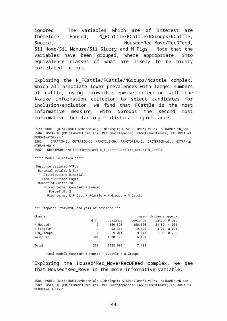
*** Estimated Variance matrix for Variance Components *** Farm 1 0.04876 Dispersn 2 0.00000 0.00000 1 2 *** Table of effects for Constant *** -0.6691 Standard error: 0.36486 *** Table of effects for Housed *** Housed 0.0000 1.0000 0.0000 1.2032 Standard error of differences: 0.3911 *** Table of effects for FCattle *** FCattle 1 2 3 4 0.0000 0.1717 -0.4264 -0.6731 Standard error of differences: Average 0.3330 Maximum 0.3876 Minimum 0.2608 Average variance of differences: 0.1133 *** Table of effects for Housed.Source *** Source Breed Buy Both Housed 0.0000 0.0000 -0.8806 -0.2403 1.0000 0.0000 -0.0607 -0.4802 Standard error of differences: Average 0.4572 Maximum 0.5820 Minimum 0.3133 Average variance of differences: 0.2177 *** Table of effects for Housed.RecChnge *** RecChnge 0.0000 1.0000 Housed 0.0000 0.0000 -0.1825 1.0000 0.0000 -0.9878 Standard error of differences: Average 0.3687 Maximum 0.4842 Minimum 0.3388 Average variance of differences: 0.1393 *** Table of effects for SSlur2 *** SSlur2 0.0000 1.0000 0.0000 -0.4288 Standard error of differences: 0.2977 *** Table of effects for Natural2 ***
44

Natural2 0.0000 1.0000 0.0000 -0.7141 Standard error of differences: 0.3534 *** Table of effects for Sheep *** Sheep 1 2 0.0000 -0.3043 Standard error of differences: 0.2317 *** Tables of means *** *** Table of predicted means for Housed *** Housed 0.0000 1.0000 -2.090 -1.096 *** Table of predicted means for FCattle *** FCattle 1 2 3 4 -1.361 -1.189 -1.787 -2.034 *** Table of predicted means for Housed.Source *** Source Breed Buy Both Housed 0.0000 -1.716 -2.597 -1.956 1.0000 -0.915 -0.976 -1.396 *** Table of predicted means for Housed.RecChnge *** RecChnge 0.0000 1.0000 Housed 0.0000 -1.998 -2.181 1.0000 -0.602 -1.590 *** Table of predicted means for SSlur2 *** SSlur2 0.0000 1.0000 -1.378 -1.807 *** Table of predicted means for Natural2 *** Natural2 0.0000 1.0000 -1.236 -1.950 *** Table of predicted means for Sheep *** Sheep 1 2 -1.440 -1.745 *** Back-transformed Means (on the original scale) *** Housed 0.0000 0.1101 1.0000 0.2506 FCattle
45

1 0.2041 2 0.2334 3 0.1434 4 0.1157 Housed 0.0000 1.0000 Source Breed 0.1524 0.2859 Buy 0.0694 0.2737 Both 0.1239 0.1985 RecChnge 0.0000 1.0000 Housed 0.0000 0.1194 0.1015 1.0000 0.3539 0.1695 SSlur2 0.0000 0.2013 1.0000 0.1410 Natural2 0.0000 0.2252 1.0000 0.1246 Sheep 1 0.1915 2 0.1487 Note: means are probabilities not expected values. 6633 VDISPLAY [PRINT=Wald] *** Wald tests for fixed effects *** Fixed term Wald statistic d.f. Wald/d.f. Chi-sq prob * Sequentially adding terms to fixed model Housed 29.54 1 29.54 <0.001 FCattle 10.11 3 3.37 0.018 Housed.Source 5.57 4 1.39 0.234 Housed.RecChnge 10.75 2 5.38 0.005 SSlur2 2.34 1 2.34 0.126 Natural2 4.13 1 4.13 0.042 Sheep 1.73 1 1.73 0.189 * Dropping individual terms from full fixed model FCattle 7.20 3 2.40 0.066 Housed.Source 5.60 4 1.40 0.231 Housed.RecChnge 8.84 2 4.42 0.012 SSlur2 2.08 1 2.08 0.150 Natural2 4.08 1 4.08 0.043 Sheep 1.73 1 1.73 0.189 * Message: chi-square distribution for Wald tests is an asymptotic approximation (i.e. for large samples) and underestimates the probabilities in other cases.
Remembering that the Wald tests are liberal, these results show no evidence for retaining Sheep and Housed.Source in the model.
Refitting the model without these factors gives the following output:
6634 GLMM [PRINT=model,monitor,components,vcovariance,means,backmeans,effects; DISTRIBUTION=binomial;\
46

6635 LINK=logit; DISPERSION=1; FIXED=Housed + FCattle + Housed.RecChnge + SSlur2 + Natural2;\6636 RANDOM=Farm; CONSTANT=estimate; FACT=9; PSE=*; MAXCYCLE=20; FMETHOD=all; CADJUST=mean]\6637 VTPos; NBINOMIAL=N_Sam ***** Generalised Linear Mixed Model Analysis ***** Method: cf Schall (1991) Biometrika Response variate: VTPos Distribution: BINOMIAL Link function: LOGIT Random model: Farm Fixed model: Constant + (((Housed + FCattle) + (Housed . RecChnge))+ SSlur2) + Natural2 * Dispersion parameter fixed at value 1.000 *** Monitoring information *** Iteration Gammas Dispersion Max change 1 1.253 1.000 1.8574E+00 2 1.585 1.000 3.3224E-01 3 1.736 1.000 1.5076E-01 4 1.757 1.000 2.1145E-02 5 1.759 1.000 1.4440E-03 6 1.759 1.000 1.6155E-04 7 1.759 1.000 1.7614E-05 *** Estimated Variance Components *** Random term Component S.e. Farm 1.759 0.221 *** Residual variance model *** Term Factor Model(order) Parameter Estimate S.e. Dispersn Identity Sigma2 1.000 FIXED *** Estimated Variance matrix for Variance Components *** Farm 1 0.04875 Dispersn 2 0.00000 0.00000 1 2 *** Table of effects for Constant *** -1.071 Standard error: 0.3036 *** Table of effects for Housed *** Housed 0.0000 1.0000 0.0000 1.3188 Standard error of differences: 0.3318 *** Table of effects for FCattle *** FCattle 1 2 3 4 0.0000 0.1309 -0.5034 -0.7694 Standard error of differences: Average 0.3248
47

Maximum 0.3815 Minimum 0.2595 Average variance of differences: 0.1077 *** Table of effects for Housed.RecChnge *** RecChnge 0.0000 1.0000 Housed 0.0000 0.0000 -0.1043 1.0000 0.0000 -0.8906 Standard error of differences: Average 0.3661 Maximum 0.4804 Minimum 0.3361 Average variance of differences: 0.1373 *** Table of effects for SSlur2 *** SSlur2 0.0000 1.0000 0.0000 -0.5229 Standard error of differences: 0.2901 *** Table of effects for Natural2 *** Natural2 0.0000 1.0000 0.0000 -0.7082 Standard error of differences: 0.3525 *** Tables of means *** *** Table of predicted means for Housed *** Housed 0.0000 1.0000 -2.024 -1.099 *** Table of predicted means for FCattle *** FCattle 1 2 3 4 -1.276 -1.145 -1.779 -2.045 *** Table of predicted means for Housed.RecChnge *** RecChnge 0.0000 1.0000 Housed 0.0000 -1.972 -2.077 1.0000 -0.653 -1.544 *** Table of predicted means for SSlur2 *** SSlur2 0.0000 1.0000 -1.300 -1.823 *** Table of predicted means for Natural2 *** Natural2 0.0000 1.0000 -1.207 -1.916 *** Back-transformed Means (on the original scale) ***
48
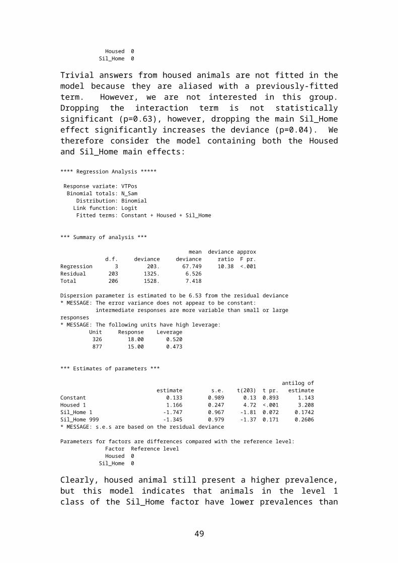
Housed 0.0000 0.1167 1.0000 0.2500 FCattle 1 0.2182 2 0.2414 3 0.1444 4 0.1145 RecChnge 0.0000 1.0000 Housed 0.0000 0.1221 0.1114 1.0000 0.3422 0.1759 SSlur2 0.0000 0.2141 1.0000 0.1391 Natural2 0.0000 0.2301 1.0000 0.1283 Note: means are probabilities not expected values. 6638 VDISPLAY [PRINT=Wald] *** Wald tests for fixed effects *** Fixed term Wald statistic d.f. Wald/d.f. Chi-sq prob * Sequentially adding terms to fixed model Housed 29.34 1 29.34 <0.001 FCattle 10.03 3 3.34 0.018 Housed.RecChnge 9.87 2 4.94 0.007 SSlur2 3.23 1 3.23 0.072 Natural2 4.04 1 4.04 0.045 * Dropping individual terms from full fixed model FCattle 9.21 3 3.07 0.027 Housed.RecChnge 7.14 2 3.57 0.028 SSlur2 3.25 1 3.25 0.071 Natural2 4.04 1 4.04 0.045 * Message: chi-square distribution for Wald tests is an asymptotic approximation (i.e. for large samples) and underestimates the probabilities in other cases.
These results show that farms on which the sampled animals were housed show statistically significantly higher (p<0.001) prevalences than those where the sampled animals were unhoused (Graph in JulyResults.xls[Multivariate Housed])
49
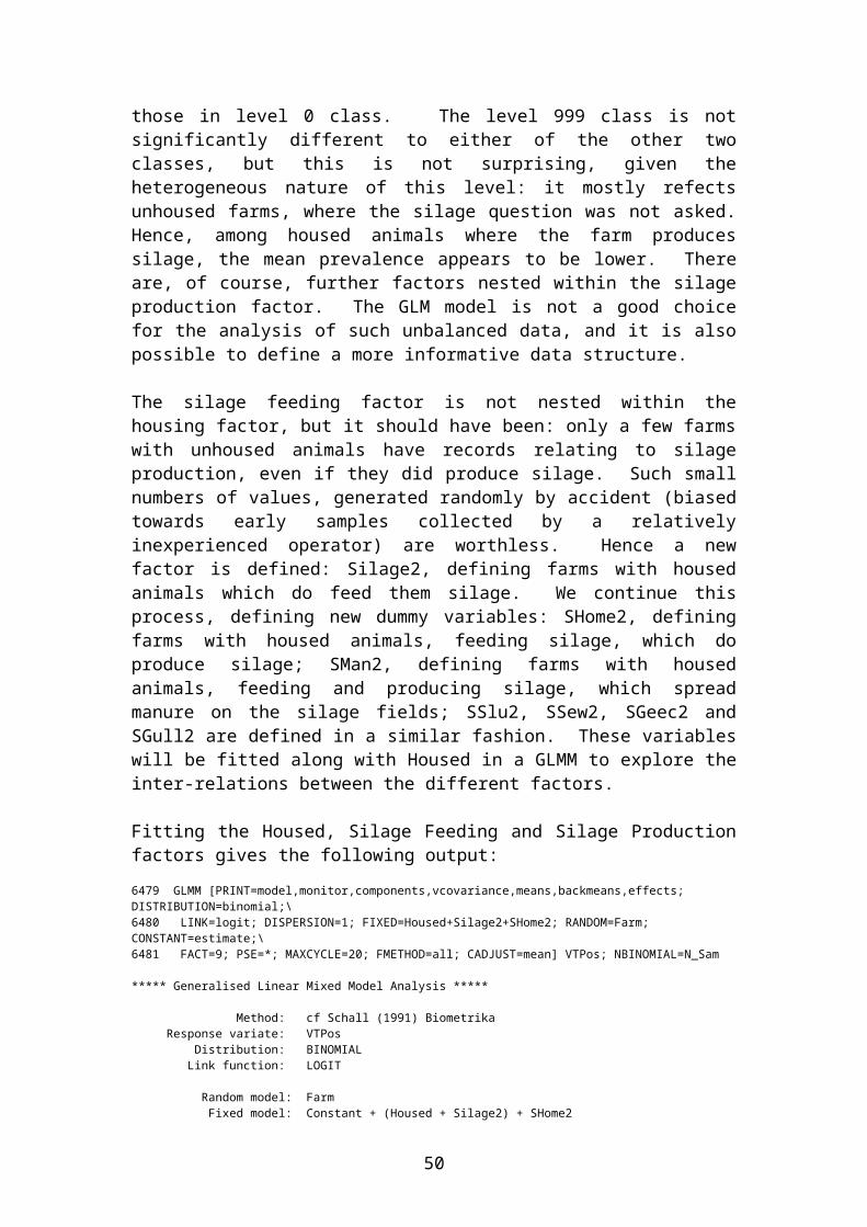
0.00
0.05
0.10
0.15
0.20
0.25
0.30
0.35
0.40
Unhoused Housed
Class of Farm
Prev
alen
ce
Plot of prevalences in housed and unhoused animals, with 95% confidence intervals.
The estimated prevalences on positive farms by housing status are as follows:
ClassMean
PrevalenceUnhoused 11.7%Housed 25.0%
The number of finishing cattle on the farm was used to define a categorical factor as follows:
Category Name Number of Finishing Cattle1 <502 50-1003 100-2004 >200
Farms which fell into categories 3 and 4 had statistically significantly lower prevalences than those in categories 1 and 2 (p=0.004).
50

0.00
0.05
0.10
0.15
0.20
0.25
0.30
0.35
0.40
FCattle 1 FCattle 2 FCattle 3 FCattle 4
Plot of prevalences in farms by FCattle category, with 95% confidence intervals.
The estimated prevalences on positive farms by number of finishing cattle are as follows:
CategoryMean
Prevalence1 21.8%2 24.1%3 14.4%4 11.5%
The variable defining whether there has been any change in diet or housing in the immediate past is significant when fitted in interaction with Housed.
0.000.050.100.150.200.250.300.350.400.450.50
Unhoused/NoChanges
Unhoused/WithChanges
Housed/NoChanges
Housed/WithChanges
Plot of prevalences in farms by Housed.RChnge category, with 95% confidence intervals.
51
0.0%
5.0%
10.0%
15.0%
20.0%
25.0%
30.0%
35.0%
40.0%
FCattle 1 FCattle 2 FCattle 3 FCattle 4

The estimated prevalences on positive farms by housing/change status are as follows:
CategoryMean
PrevalenceUnhoused/No Changes 12.2%
Unhoused/With Changes 11.1%Housed/No Changes 34.2%
Housed/With Changes 17.6%
There is no significant effect due to changes among unhoused animals (p=0.76). However, the prevalence among housed animals with recent changes is higher although not statistically significant (p=0.26), while the prevalence among housed animals without recent changes is significantly higher again (p=0.007). This can be interpreted as a ‘build-up’ effect: housing increases the prevalence, and the presence of a recent change implies that the housing effect will have had a shorter period of time to take effect. It should be remembered that this factor could reflect either changes in diet or changes in location: although it is tempting to interpret the results in terms of the change in location, this uncertainty should be borne in mind.
0.00
0.05
0.10
0.15
0.20
0.25
0.30
0.35
Natural Water Source Other
Plot of prevalences in farms by water source, with 95% confidence intervals.
The estimated prevalences on positive farms by water source are as follows:
CategoryMean
PrevalenceNatural Water 12.8%
Other 23.0%
Farms on which unhoused animals have access to a natural water supply have a lower prevalence (p=0.045) than on other farms.
52

0.00
0.05
0.10
0.15
0.20
0.25
0.30
No Slurry Spread Slurry Spread
Plot of prevalences in farms by Slurry Spreading status, with 95% confidence intervals.
The estimated prevalences on positive farms by slurry spreading status are as follows:
CategoryMean
PrevalenceNo Silage Grown 21.4%
Silage Grown 13.9%
Farms on which slurry is spread on the silage fields have a lower prevalence than those farms on which no slurry is spread. This difference is not statistically significant (p=0.07) but would seem worth reporting.
Having fitted all the likely explanatory variables in the multifactor model, we now return to explore the effect that the inclusion of these factors may have on the fit of the structural factors.
Fitting Division and Division.Housed gives the following output:
7122 GLMM [PRINT=model,monitor,components,vcovariance,means,backmeans,effects; DISTRIBUTION=binomial;\7123 LINK=logit; DISPERSION=1; FIXED=Housed + FCattle + Housed.RecChnge + SSlur2+ Natural2+Division+Division.Housed;\7124 RANDOM=Farm; CONSTANT=estimate; FACT=9; PSE=*; MAXCYCLE=20; FMETHOD=all; CADJUST=mean]\7125 VTPos; NBINOMIAL=N_Sam ***** Generalised Linear Mixed Model Analysis ***** Method: cf Schall (1991) Biometrika Response variate: VTPos Distribution: BINOMIAL Link function: LOGIT Random model: Farm Fixed model: Constant + (((((Housed + FCattle) + (Housed . RecChnge)) + SSlur2) + Natural2) + Division) + (Housed . Division) * Dispersion parameter fixed at value 1.000
53

*** Monitoring information *** Iteration Gammas Dispersion Max change 1 1.292 1.000 1.7250E+00 2 1.533 1.000 2.4051E-01 3 1.678 1.000 1.4561E-01 4 1.697 1.000 1.9120E-02 5 1.699 1.000 1.2743E-03 6 1.699 1.000 1.3341E-04 7 1.699 1.000 1.3609E-05 *** Estimated Variance Components *** Random term Component S.e. Farm 1.699 0.221 *** Residual variance model *** Term Factor Model(order) Parameter Estimate S.e. Dispersn Identity Sigma2 1.000 FIXED *** Estimated Variance matrix for Variance Components *** Farm 1 0.04885 Dispersn 2 0.00000 0.00000 1 2 *** Table of effects for Constant *** -1.232 Standard error: 0.4404 *** Table of effects for Housed *** Housed 0.0000 1.0000 0.0000 1.3835 Standard error of differences: 0.5199 *** Table of effects for FCattle *** FCattle 1 2 3 4 0.0000 0.2010 -0.3886 -0.6241 Standard error of differences: Average 0.3262 Maximum 0.3793 Minimum 0.2614 Average variance of differences: 0.1085 *** Table of effects for Housed.RecChnge *** RecChnge 0.0000 1.0000 Housed 0.0000 0.0000 -0.2138 1.0000 0.0000 -0.8995 Standard error of differences: Average 0.3702 Maximum 0.4860 Minimum 0.3347 Average variance of differences: 0.1404
54

*** Table of effects for SSlur2 *** SSlur2 0.0000 1.0000 0.0000 -0.3293 Standard error of differences: 0.3029 *** Table of effects for Natural2 *** Natural2 0.0000 1.0000 0.0000 -0.6814 Standard error of differences: 0.3534 *** Table of effects for Division *** Division Central Highland Islands North East South East 0.0000 0.6400 0.4473 0.1987 0.5044 Division South West -0.4383 Standard error of differences: Average 0.6037 Maximum 0.7070 Minimum 0.4892 Average variance of differences: 0.3678 *** Table of effects for Housed.Division *** Division Central Highland Islands North East South East Housed 0.0000 0.0000 0.0000 0.0000 0.0000 0.0000 1.0000 0.0000 1.1292 -1.7037 -0.1396 -0.4355 Division South West Housed 0.0000 0.0000 1.0000 -0.0928 Standard error of differences: Average 0.8699 Maximum 1.378 Minimum 0.6133 Average variance of differences: 0.8114 *** Tables of means *** *** Table of predicted means for Housed *** Housed 0.0000 1.0000 -1.822 -0.988 *** Table of predicted means for FCattle *** FCattle 1 2 3 4 -1.202 -1.001 -1.591 -1.826 *** Table of predicted means for Housed.RecChnge *** RecChnge 0.0000 1.0000 Housed 0.0000 -1.715 -1.929 1.0000 -0.538 -1.438
55

*** Table of predicted means for SSlur2 *** SSlur2 0.0000 1.0000 -1.240 -1.570 *** Table of predicted means for Natural2 *** Natural2 0.0000 1.0000 -1.064 -1.746 *** Table of predicted means for Division *** Division Central Highland Islands North East South East -1.527 -0.322 -1.931 -1.398 -1.240 Division South West -2.011 *** Table of predicted means for Housed.Division *** Division Central Highland Islands North East South East Housed 0.0000 -2.047 -1.407 -1.600 -1.848 -1.543 1.0000 -1.006 0.763 -2.263 -0.947 -0.937 Division South West Housed 0.0000 -2.485 1.0000 -1.538 *** Back-transformed Means (on the original scale) *** Housed 0.0000 0.1392 1.0000 0.2713 FCattle 1 0.2311 2 0.2688 3 0.1693 4 0.1387 RecChnge 0.0000 1.0000 Housed 0.0000 0.1526 0.1269 1.0000 0.3686 0.1919 SSlur2 0.0000 0.2244 1.0000 0.1723 Natural2 0.0000 0.2565 1.0000 0.1486 Division Central 0.1785 Highland 0.4202 Islands 0.1266 North East 0.1982 South East 0.2244 South West 0.1180
56

Housed 0.0000 1.0000 Division Central 0.1144 0.2677 Highland 0.1967 0.6820 Islands 0.1680 0.0943 North East 0.1361 0.2794 South East 0.1762 0.2814 South West 0.0769 0.1769 Note: means are probabilities not expected values.
7106 VDISPLAY [PRINT=Wald] *** Wald tests for fixed effects *** Fixed term Wald statistic d.f. Wald/d.f. Chi-sq prob * Sequentially adding terms to fixed model Housed 29.73 1 29.73 <0.001 FCattle 10.16 3 3.39 0.017 Housed.RecChnge 10.11 2 5.05 0.006 SSlur2 3.30 1 3.30 0.069 Natural2 4.12 1 4.12 0.042 Division 12.27 5 2.45 0.031 Housed.Division 4.78 5 0.96 0.443 * Dropping individual terms from full fixed model FCattle 7.24 3 2.41 0.065 Housed.RecChnge 7.65 2 3.82 0.022 SSlur2 1.18 1 1.18 0.277 Natural2 3.72 1 3.72 0.054 Housed.Division 4.78 5 0.96 0.443 * Message: chi-square distribution for Wald tests is an asymptotic approximation (i.e. for large samples) and underestimates the probabilities in other cases.
Hence, although Housed.Division is not significant, there is still significant evidence of geographical variability unexplained by the fitted epidemiological factors (in fact, the geographical distinctions are more clear after the effects of the other factors have been removed).
Fitting Manage_O gives the following Wald statistics:7111 VDISPLAY [PRINT=Wald] *** Wald tests for fixed effects *** Fixed term Wald statistic d.f. Wald/d.f. Chi-sq prob * Sequentially adding terms to fixed model Housed 29.16 1 29.16 <0.001 FCattle 9.98 3 3.33 0.019 Housed.RecChnge 9.82 2 4.91 0.007 SSlur2 3.21 1 3.21 0.073 Natural2 4.01 1 4.01 0.045 Manage_O 0.93 2 0.46 0.630 * Dropping individual terms from full fixed model FCattle 9.05 3 3.02 0.029 Housed.RecChnge 7.24 2 3.62 0.027 SSlur2 3.50 1 3.50 0.062 Natural2 3.90 1 3.90 0.048
57

Manage_O 0.93 2 0.46 0.630 * Message: chi-square distribution for Wald tests is an asymptotic approximation (i.e. for large samples) and underestimates the probabilities in other cases.
Fitting Housed.Manage_O gives the following Wald statistics:
7116 VDISPLAY [PRINT=Wald] *** Wald tests for fixed effects *** Fixed term Wald statistic d.f. Wald/d.f. Chi-sq prob * Sequentially adding terms to fixed model Housed 29.36 1 29.36 <0.001 FCattle 10.10 3 3.37 0.018 Housed.RecChnge 9.97 2 4.98 0.007 SSlur2 3.26 1 3.26 0.071 Natural2 4.01 1 4.01 0.045 Housed.Manage_O 6.25 4 1.56 0.181 * Dropping individual terms from full fixed model FCattle 10.47 3 3.49 0.015 Housed.RecChnge 7.61 2 3.80 0.022 SSlur2 3.53 1 3.53 0.060 Natural2 4.02 1 4.02 0.045 Housed.Manage_O 6.25 4 1.56 0.181 * Message: chi-square distribution for Wald tests is an asymptotic approximation (i.e. for large samples) and underestimates the probabilities in other cases.
Hence there is no evidence of Manage_O or its interaction with Housed having any significant effect on the prevalence.
Fitting Sam_Mon (which was highly significant in the univariate analysis) gives the following output:7126 GLMM [PRINT=model,monitor,components,vcovariance,means,backmeans,effects; DISTRIBUTION=binomial;\7127 LINK=logit; DISPERSION=1; FIXED=Housed + FCattle + Housed.RecChnge + SSlur2+ Natural2+Sam_Mon+Sam_Mon.Housed;\7128 RANDOM=Farm; CONSTANT=estimate; FACT=9; PSE=*; MAXCYCLE=20; FMETHOD=all; CADJUST=mean]\7129 VTPos; NBINOMIAL=N_Sam ***** Generalised Linear Mixed Model Analysis ***** Method: cf Schall (1991) Biometrika Response variate: VTPos Distribution: BINOMIAL Link function: LOGIT Random model: Farm Fixed model: Constant + (((((Housed + FCattle) + (Housed . RecChnge)) + SSlur2) + Natural2) + Sam_Mon) + (Housed . Sam_Mon) * Dispersion parameter fixed at value 1.000 *** Monitoring information *** Iteration Gammas Dispersion Max change 1 1.241 1.000 1.7883E+00 2 1.548 1.000 3.0736E-01 3 1.701 1.000 1.5289E-01 4 1.722 1.000 2.1058E-02 5 1.724 1.000 1.4655E-03
58

6 1.724 1.000 1.5810E-04 7 1.724 1.000 1.6533E-05 *** Estimated Variance Components *** Random term Component S.e. Farm 1.724 0.228 *** Residual variance model *** Term Factor Model(order) Parameter Estimate S.e. Dispersn Identity Sigma2 1.000 FIXED *** Estimated Variance matrix for Variance Components *** Farm 1 0.05218 Dispersn 2 0.00000 0.00000 1 2 *** Table of effects for Constant *** -2.230 Standard error: 1.3511 *** Table of effects for Housed *** Housed 0.0000 1.0000 0.000 2.929 Standard error of differences: 1.267 *** Table of effects for FCattle *** FCattle 1 2 3 4 0.0000 0.1277 -0.6122 -0.7928 Standard error of differences: Average 0.3353 Maximum 0.3965 Minimum 0.2706 Average variance of differences: 0.1147 *** Table of effects for Housed.RecChnge *** RecChnge 0.0000 1.0000 Housed 0.0000 0.0000 -0.0109 1.0000 0.0000 -0.9641 Standard error of differences: Average 0.4218 Maximum 0.5547 Minimum 0.3789 Average variance of differences: 0.1824 *** Table of effects for SSlur2 *** SSlur2 0.0000 1.0000 0.0000 -0.5271 Standard error of differences: 0.3023
59

*** Table of effects for Natural2 *** Natural2 0.0000 1.0000 0.0000 -0.6120 Standard error of differences: 0.3729 *** Table of effects for Sam_Mon *** Sam_Mon Jan Feb Mar Apr May 0.0000 -1.1247 0.2774 -0.0039 1.1748 Sam_Mon Jun Jul Aug Sep Oct 1.3308 1.3849 1.4567 0.8369 0.5001 Sam_Mon Nov Dec -0.2282 -0.2707 Standard error of differences: Average 1.259 Maximum 2.157 Minimum 0.5449 Average variance of differences: 1.816 *** Table of effects for Housed.Sam_Mon *** Sam_Mon Jan Feb Mar Apr May Housed 0.0000 * * 0.0000 0.0000 0.0000 1.0000 0.0000 0.0000 -0.6260 -0.5438 -0.8902 Sam_Mon Jun Jul Aug Sep Oct Housed 0.0000 0.0000 0.0000 0.0000 0.0000 0.0000 1.0000 * -2.7419 -1.5238 -4.0927 -1.4113 Sam_Mon Nov Dec Housed 0.0000 0.0000 * 1.0000 0.0000 0.0000 Standard error of differences: Average 1.655 Maximum 2.152 Minimum 0.9070 Average variance of differences: 2.805 *** Tables of means *** *** Table of predicted means for Housed *** Housed 0.0000 1.0000 * * *** Table of predicted means for FCattle *** FCattle 1 2 3 4 -1.726 -1.599 -2.338 -2.519 *** Table of predicted means for Housed.RecChnge *** RecChnge 0.0000 1.0000 Housed 0.0000 * *
60

1.0000 * * *** Table of predicted means for SSlur2 *** SSlur2 0.0000 1.0000 -1.782 -2.309 *** Table of predicted means for Natural2 *** Natural2 0.0000 1.0000 -1.740 -2.352 *** Table of predicted means for Sam_Mon *** Sam_Mon Jan Feb Mar Apr May Jun Jul Aug * * -1.934 -2.174 -1.169 * -1.885 -1.204 Sam_Mon Sep Oct Nov Dec -3.108 -2.104 -2.127 * *** Table of predicted means for Housed.Sam_Mon *** Sam_Mon Jan Feb Mar Apr May Jun Jul Housed 0.0000 * * -2.847 -3.129 -1.950 -1.794 -1.740 1.0000 -0.673 -1.797 -1.021 -1.220 -0.388 * -2.030 Sam_Mon Aug Sep Oct Nov Dec Housed 0.0000 -1.668 -2.288 -2.625 -3.353 * 1.0000 -0.740 -3.928 -1.584 -0.901 -0.943 *** Back-transformed Means (on the original scale) *** Housed 0.0000 * 1.0000 * FCattle 1 0.1511 2 0.1682 3 0.0880 4 0.0745 RecChnge 0.0000 1.0000 Housed 0.0000 * * 1.0000 * * SSlur2 0.0000 0.1440 1.0000 0.0904 Natural2 0.0000 0.1494 1.0000 0.0869 Sam_Mon Jan * Feb * Mar 0.1263 Apr 0.1021 May 0.2370 Jun *
61

Jul 0.1319 Aug 0.2308 Sep 0.0428 Oct 0.1087 Nov 0.1065 Dec * Housed 0.0000 1.0000 Sam_Mon Jan * 0.3379 Feb * 0.1422 Mar 0.0548 0.2648 Apr 0.0419 0.2279 May 0.1246 0.4042 Jun 0.1426 * Jul 0.1493 0.1161 Aug 0.1587 0.3231 Sep 0.0921 0.0193 Oct 0.0676 0.1703 Nov 0.0338 0.2889 Dec * 0.2802 Note: means are probabilities not expected values.
7121 VDISPLAY [PRINT=Wald] *** Wald tests for fixed effects *** Fixed term Wald statistic d.f. Wald/d.f. Chi-sq prob * Sequentially adding terms to fixed model Housed 29.42 1 29.42 <0.001 FCattle 10.20 3 3.40 0.017 Housed.RecChnge 9.95 2 4.97 0.007 SSlur2 3.30 1 3.30 0.069 Natural2 4.00 1 4.00 0.045 Sam_Mon 14.10 11 1.28 0.227 Housed.Sam_Mon 9.12 7 1.30 0.244 * Dropping individual terms from full fixed model FCattle 10.76 3 3.59 0.013 Housed.RecChnge 6.48 2 3.24 0.039 SSlur2 3.04 1 3.04 0.081 Natural2 2.69 1 2.69 0.101 Housed.Sam_Mon 9.12 7 1.30 0.244 * Message: chi-square distribution for Wald tests is an asymptotic approximation (i.e. for large samples) and underestimates the probabilities in other cases.
Neither Sam_Mon or Housed.Sam_Mon are statistically significant. Hence, the explanatory variables (particularly Housed) have explained most of the variability that was assigned to Month in the univariate analysis. We confirm this by refitting the model without any of the housing terms:
7134 VDISPLAY [PRINT=Wald] *** Wald tests for fixed effects *** Fixed term Wald statistic d.f. Wald/d.f. Chi-sq prob * Sequentially adding terms to fixed model FCattle 4.89 3 1.63 0.180 SSlur2 0.01 1 0.01 0.943 Natural2 21.19 1 21.19 <0.001 Sam_Mon 24.74 11 2.25 0.010
62
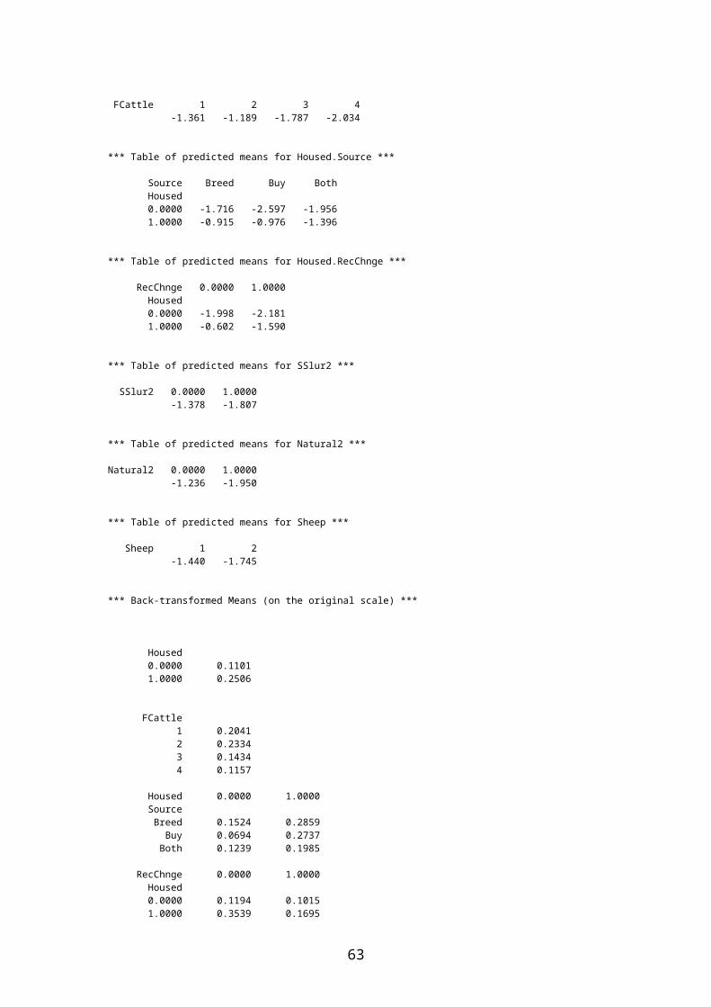
* Dropping individual terms from full fixed model FCattle 8.12 3 2.71 0.044 SSlur2 2.19 1 2.19 0.139 Natural2 12.75 1 12.75 <0.001 Sam_Mon 24.74 11 2.25 0.010 * Message: chi-square distribution for Wald tests is an asymptotic approximation (i.e. for large samples) and underestimates the probabilities in other cases.
This output confirms that the month to month variability is almost completely explained by the Housed terms.
Reviewing the pattern of housing of animals over the year we see the following pattern:
0
0.2
0.4
0.6
0.8
1
Janu
ary
Febru
ary
March
April
MayJu
ne July
Augus
t
Septem
ber
Octobe
r
Novembe
r
Decembe
r
Month
Prop
ortio
n G
roup
s Ho
used
Proportion of Sampling Groups Housed, by Month, with 95% Confidence Intervals.
In the univariate analysis, the months exhibiting a lower prevalence were identified as June to October. June to September are the months with the lowest proportion of animals housed, while in October, although a higher proportion of groups are housed, the ‘recent change’ factor is likely to operate to reduce the shedding prevalence.
Fitting Sam_Year and Sam_Year.Housed to the data gives rise to the following summary statistics:
7139 VDISPLAY [PRINT=Wald] *** Wald tests for fixed effects *** Fixed term Wald statistic d.f. Wald/d.f. Chi-sq prob * Sequentially adding terms to fixed model
63

Housed 29.01 1 29.01 <0.001 FCattle 9.95 3 3.32 0.019 Housed.RecChnge 9.79 2 4.89 0.007 SSlur2 3.19 1 3.19 0.074 Natural2 3.98 1 3.98 0.046 Sam_Year 1.00 2 0.50 0.606 Housed.Sam_Year 2.33 2 1.17 0.312 * Dropping individual terms from full fixed model FCattle 8.30 3 2.77 0.040 Housed.RecChnge 4.87 2 2.43 0.088 SSlur2 3.30 1 3.30 0.069 Natural2 3.44 1 3.44 0.064 Housed.Sam_Year 2.33 2 1.17 0.312 * Message: chi-square distribution for Wald tests is an asymptotic approximation (i.e. for large samples) and underestimates the probabilities in other cases.
There is no evidence of any year-on-year trend in prevalence in either housed or unhoused animals.
Returning to the model with the explanatory factors and animal health division, the prevalences by area, after adjusting for the significant explanatory variables, are given by fitting the following model:7140 GLMM [PRINT=model,monitor,components,vcovariance,means,backmeans,effects; DISTRIBUTION=binomial;\7141 LINK=logit; DISPERSION=1; FIXED=Housed+ FCattle + Housed.RecChnge+SSlur2+ Natural2+Division;\7142 RANDOM=Farm; CONSTANT=estimate; FACT=9; PSE=*; MAXCYCLE=20; FMETHOD=all; CADJUST=mean]\7143 VTPos; NBINOMIAL=N_Sam ***** Generalised Linear Mixed Model Analysis ***** Method: cf Schall (1991) Biometrika Response variate: VTPos Distribution: BINOMIAL Link function: LOGIT Random model: Farm Fixed model: Constant + ((((Housed + FCattle) + (Housed . RecChnge)) + SSlur2) + Natural2) + Division * Dispersion parameter fixed at value 1.000 *** Monitoring information *** Iteration Gammas Dispersion Max change 1 1.237 1.000 1.7843E+00 2 1.533 1.000 2.9627E-01 3 1.666 1.000 1.3312E-01 4 1.685 1.000 1.8695E-02 5 1.686 1.000 1.2612E-03 6 1.686 1.000 1.3440E-04 7 1.686 1.000 1.3954E-05 *** Estimated Variance Components *** Random term Component S.e. Farm 1.686 0.217 *** Residual variance model *** Term Factor Model(order) Parameter Estimate S.e. Dispersn Identity Sigma2 1.000 FIXED
64

*** Estimated Variance matrix for Variance Components *** Farm 1 0.04689 Dispersn 2 0.00000 0.00000 1 2 *** Table of effects for Constant *** -1.178 Standard error: 0.3600 *** Table of effects for Housed *** Housed 0.0000 1.0000 0.0000 1.2921 Standard error of differences: 0.3288 *** Table of effects for FCattle *** FCattle 1 2 3 4 0.0000 0.2252 -0.4122 -0.6472 Standard error of differences: Average 0.3220 Maximum 0.3765 Minimum 0.2586 Average variance of differences: 0.1058 *** Table of effects for Housed.RecChnge *** RecChnge 0.0000 1.0000 Housed 0.0000 0.0000 -0.1707 1.0000 0.0000 -0.8901 Standard error of differences: Average 0.3654 Maximum 0.4806 Minimum 0.3326 Average variance of differences: 0.1369 *** Table of effects for SSlur2 *** SSlur2 0.0000 1.0000 0.0000 -0.3338 Standard error of differences: 0.2957 *** Table of effects for Natural2 *** Natural2 0.0000 1.0000 0.0000 -0.7004 Standard error of differences: 0.3498 *** Table of effects for Division *** Division Central Highland Islands North East South East 0.0000 1.0762 0.1254 0.1065 0.1952 Division South West
65
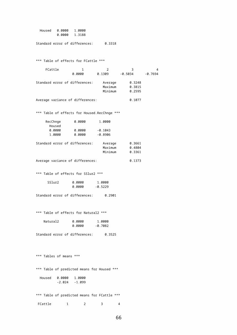
-0.4932 Standard error of differences: Average 0.4146 Maximum 0.5626 Minimum 0.2942 Average variance of differences: 0.1788 *** Tables of means *** *** Table of predicted means for Housed *** Housed 0.0000 1.0000 -1.821 -0.888 *** Table of predicted means for FCattle *** FCattle 1 2 3 4 -1.146 -0.921 -1.558 -1.793 *** Table of predicted means for Housed.RecChnge *** RecChnge 0.0000 1.0000 Housed 0.0000 -1.735 -1.906 1.0000 -0.443 -1.333 *** Table of predicted means for SSlur2 *** SSlur2 0.0000 1.0000 -1.188 -1.521 *** Table of predicted means for Natural2 *** Natural2 0.0000 1.0000 -1.004 -1.705 *** Table of predicted means for Division *** Division Central Highland Islands North East South East -1.523 -0.447 -1.398 -1.416 -1.328 Division South West -2.016 *** Back-transformed Means (on the original scale) *** Housed 0.0000 0.1393 1.0000 0.2914 FCattle 1 0.2412 2 0.2848 3 0.1739 4 0.1427 RecChnge 0.0000 1.0000 Housed 0.0000 0.1499 0.1294 1.0000 0.3909 0.2086 SSlur2
66

0.0000 0.2337 1.0000 0.1792 Natural2 0.0000 0.2681 1.0000 0.1538 Division Central 0.1790 Highland 0.3902 Islands 0.1982 North East 0.1952 South East 0.2095 South West 0.1175 Note: means are probabilities not expected values.
0
0.1
0.2
0.3
0.4
0.5
0.6
0.7
Division Central
Division Highland
Division Islands
DivisionNorth East
DivisionSouth East
DivisionSouthWest
Plot of prevalences by animal health division, with 95% confidence intervals.
The mean prevalence in Highland division appears to be significantly higher than those in Central, Islands, North-East and South-East (p=0.02), while the prevalences in these regions are significantly higher than that in the South-West (p=0.03). These trends match those seen in the univariate analysis.
Reviewing the fit of the model, plotting the observed and expected fractions of positive pats for the 207 data included in the model gives the following plot:
67

0
0.1
0.2
0.3
0.4
0.5
0.6
0.7
0.8
0.9
1
0 0.2 0.4 0.6 0.8 1
Observed Fraction
Mod
el P
roba
bilit
y
Plot of observed and fitted fractional prevalences.
Overall, the fit looks fairly reasonable, with a few minor outliers. The only serious lack of fit occurs for maximal prevalences, where the fitted model will always be smaller than an observed 100% shedding rate. Even this cluster of negative residuals looks likely to be of negligible effect. To assess this more formally, we examine a residual plot for the model. The residuals and fitted values from the model (based on the inclusion only of fixed effects) are recovered by refitting the model using the marginal method of Breslow & Clayton (1993) and then recovering the residuals using
VKEEP [RES=Residuals;FIT=Fitted].
The resulting fitted values are converted back onto the proportion scale using the inverse of the logit function, and the resulting plot is shown below:
68

-1.5
-1
-0.5
0
0.5
1
1.5
0 0.2 0.4 0.6 0.8 1
Fitted Fraction
Resi
dual
Plot of residual against model fit (random effects model).
The histogram of these residuals should also be examined.
Residuals (Random)
Freq
uenc
y
1.20.80.40.0-0.4-0.8
40
30
20
10
0
Histogram of Residuals (Random)
Histogram of residuals (random effects model).
69

The pattern of the residuals against the fitted value is fairly typical of this class of residuals. The histogram is sufficiently symmetric for the fit of the model to be regarded as acceptable, although there may be some evidence of sub-populations in the histogram. Interpretation of these residuals is problematic. To fully evaluate the fit of the model, we examine the deviance residuals from the equivalent fixed effect model with overdispersion. This model is close in its properties to the mixed model, and the deviance residuals are easier to interpret. The residuals are recovered using the RKEEP command, using the default residual settings in RKEEP and MODEL.
The resulting fitted values are converted back onto the proportion scale using the inverse of the logit function, and the resulting plot is shown below:
-2.5
-2
-1.5
-1
-0.5
0
0.5
1
1.5
2
2.5
3
0 0.2 0.4 0.6 0.8 1
Fitted Fraction
Resi
dual
Plot of residual against model fit (fixed effects model).
The histogram of these residuals should also be examined.
70

Residuals (Fixed)
Freq
uenc
y
2.251.500.750.00-0.75-1.50
30
25
20
15
10
5
0
Histogram of Residuals (Fixed)
Histogram of residuals (fixed effects model).
These graphics are much more easy to interpret. The main peculiarities appear to be a clustering of moderately negative residuals associated with observed fractional prevalences in the range 20-30%, and a slightly disproportionate number of high (>2) residuals. The latter are, however, drawn from a wide range of observations with different prevalences. It is, indeed, plausible that the latter peculiarity is a side-effect of the former, since if the residual histogram is visualised as a confounding of two subpopulations, one centred on a value slightly larger than zero, and the other on a value around –0.75, both sub-populations appear reasonably normally distributed in the dataset. No points have been highlighted by Genstat as exhibiting high leverage. Calculating Cook’s statistics for each observation to identify observations which combine both large residuals with high leverage, no particular pattern is apparent. No sub-population of the dataset appears to be having a consistently strong effect on the model.
71

Plotting the Cook’s statistics against the various explanatory factors shows no particular trend. Only one point stands out in this exercise: the point (Farm 515) with the largest Cook’s statistic appears as an outlier in both the Highland level of the Division factor and in the Housed with recent change level of the Housed.RecChnge interaction term. However, removing this farm from the model has a negligible effect on the residuals (and on the model and associated p-values in general).
The subpopulation of residuals correspond to a group of farms with lower than expected shedding levels. The predicted prevalence is in the range 20%-30%, while that observed is much lower: typically only one or two positive pats. Examination of the properties of these observations shows some pattern. They tend to be observations from farms which lack any of the obvious risk factors, or, if they do, these are off-set by other, protective factors. Hence, their fitted risk is close to the estimated mean, which is higher than the actual prevalence seen on these farms. This does not appear to be a response to the inclusion of any specific factor in the model (given the lack of evidence for significant leverage in the model), rather, it is a property of the response distribution, where on some farms there are much fewer positive pats detected than on apparently similar farms. This could reflect some unidentified and hence unmodelled explanatory factor, or some peculiarity of the distribution which describes the random terms. It is difficult to interpret such effects in purely random terms: the most obvious aspect of the raw data, namely the apparent ‘bulge’ at high prevalences, can be explained by various aspects of contagion models (such as the stochastic threshold theorem) or by hypothesising the existence of hyper-shedding cattle. It is more
72
VTPos
Fitted values suitably transformed
60
1.0
40
0.5
0.0
2.5
1.5
2.0
3.0
12010080
Cook's statistics

difficult to conceptualise a distributional effect which gives rise to a smaller population at moderate prevalences.
If this sub-population does reflect a genuine and unidentified explanatory factor, at least it is an unidentified protective factor rather than an unidentified risk factor. Examination of the residuals would suggest that the residuals, although less than perfect, are not sufficiently asymmetric to undermine the asymptotic assumptions which underlie the calculation of standard errors and p-values. Hence, the results reported in this document are still valid, and can be reported with confidence.
73

Analysing Bernoulli data (absence or presence of farm level infection)
Initially, the effect of the descriptive variables (Division, Sam_Month, Manage_O) will be assessed:
5559 MODEL [DISTRIBUTION=binomial; LINK=logit; DISPERSION=1] VFarmPos; NBINOMIAL=N_Bin5560 FIT [PRINT=model,summary,estimates; CONSTANT=estimate; FPROB=yes; TPROB=yes; FACT=9]\5561 Manage_O ***** Regression Analysis ***** Response variate: VFarmPos Binomial totals: N_Bin Distribution: Binomial Link function: Logit Fitted terms: Constant, Manage_O *** Summary of analysis *** mean deviance approx d.f. deviance deviance ratio chi prRegression 3 1.0 0.328 0.33 0.805Residual 948 996.0 1.051Total 951 997.0 1.048* MESSAGE: ratios are based on dispersion parameter with value 1 Dispersion parameter is fixed at 1.00* MESSAGE: The following units have high leverage: Unit Response Leverage 221 0.00 0.1845 351 0.00 0.1845 *** Estimates of parameters *** antilog of estimate s.e. t(*) t pr. estimateConstant -1.291 0.196 -6.58 <.001 0.2750Manage_O Beef 0.010 0.220 0.05 0.963 1.010Manage_O Other 0.032 0.260 0.12 0.903 1.032Manage_O Mixed -4.27 6.95 -0.61 0.539 0.01400* MESSAGE: s.e.s are based on dispersion parameter with value 1 Parameters for factors are differences compared with the reference level: Factor Reference level Manage_O Dairy
Manage_O shows no significant effects. Division shows more interesting effects.
5562 MODEL [DISTRIBUTION=binomial; LINK=logit; DISPERSION=1] VFarmPos; NBINOMIAL=N_Bin5563 FIT [PRINT=model,summary,estimates; CONSTANT=estimate; FPROB=yes; TPROB=yes; FACT=9]\5564 Division
5564............................................................................ ***** Regression Analysis ***** Response variate: VFarmPos Binomial totals: N_Bin Distribution: Binomial Link function: Logit Fitted terms: Constant, Division
74

*** Summary of analysis *** mean deviance approx d.f. deviance deviance ratio chi prRegression 5 7.9 1.580 1.58 0.162Residual 946 989.1 1.046Total 951 997.0 1.048* MESSAGE: ratios are based on dispersion parameter with value 1 Dispersion parameter is fixed at 1.00* MESSAGE: The error variance does not appear to be constant: large responses are more variable than small responses *** Estimates of parameters *** antilog of estimate s.e. t(*) t pr. estimateConstant -1.106 0.170 -6.52 <.001 0.3309Division Highland -0.612 0.336 -1.82 0.069 0.5423Division Islands -0.475 0.339 -1.40 0.161 0.6221Division North East -0.005 0.232 -0.02 0.982 0.9947Division South East 0.017 0.260 0.07 0.948 1.017Division South West -0.354 0.236 -1.50 0.133 0.7020* MESSAGE: s.e.s are based on dispersion parameter with value 1 Parameters for factors are differences compared with the reference level: Factor Reference level Division Central
Overall, there is no statistically significant evidence of any differences in the levels of farm prevalence in different areas of Scotland. The prevalence in the Central, North-East and South-East are all comparable, with the prevalence in the South-West being lower, and that in the Highlands and the Islands lower still.
0%
5%
10%
15%
20%
25%
30%
35%
Central Highlands Islands NE SE SW
Plot of farm prevalences by animal health division (univariate analysis), with 95% confidence intervals.
75

The estimated prevalences of positive farms in different divisions are as follows:
Central 25%Highlands 15%Islands 17%NE 25%SE 25%SW 19%
These results are interesting, noting in particular that the high animal prevalence in the Highlands is matched with a low farm prevalence, but no trend is apparent when the animal and farm prevalences are plotted by Division, and in general, it must be stressed that the farm prevalence effects are not statistically significant.
Examining Sampling Month,
5602 MODEL [DISTRIBUTION=binomial; LINK=logit; DISPERSION=1] VFarmPos; NBINOMIAL=N_Bin5603 FIT [PRINT=model,summary,estimates; CONSTANT=estimate; FPROB=yes; TPROB=yes; FACT=9]\5604 Sam_Mon 5604............................................................................ ***** Regression Analysis ***** Response variate: VFarmPos Binomial totals: N_Bin Distribution: Binomial Link function: Logit Fitted terms: Constant, Sam_Mon *** Summary of analysis *** mean deviance approx d.f. deviance deviance ratio chi prRegression 11 19.0 1.731 1.73 0.060Residual 940 978.0 1.040Total 951 997.0 1.048* MESSAGE: ratios are based on dispersion parameter with value 1 Dispersion parameter is fixed at 1.00* MESSAGE: The error variance does not appear to be constant: large responses are more variable than small responses *** Estimates of parameters *** antilog of estimate s.e. t(*) t pr. estimateConstant -2.031 0.376 -5.40 <.001 0.1311Sam_Mon Feb 0.292 0.481 0.61 0.544 1.340Sam_Mon Mar 0.784 0.435 1.80 0.071 2.190Sam_Mon Apr 0.340 0.475 0.71 0.475 1.405Sam_Mon May 1.051 0.432 2.43 0.015 2.860Sam_Mon Jun 0.502 0.485 1.04 0.300 1.652Sam_Mon Jul 1.010 0.465 2.17 0.030 2.745Sam_Mon Aug 0.915 0.463 1.97 0.048 2.496Sam_Mon Sep 1.030 0.466 2.21 0.027 2.801Sam_Mon Oct 0.696 0.452 1.54 0.123 2.007Sam_Mon Nov 1.364 0.466 2.93 0.003 3.910Sam_Mon Dec 0.677 0.546 1.24 0.215 1.968* MESSAGE: s.e.s are based on dispersion parameter with value 1
76

Parameters for factors are differences compared with the reference level: Factor Reference level Sam_Mon Jan 5605 RKEEP ; ESTIMATES=Est; VCOVARIANCE=Var
Overall, there is no statistically significant evidence of any differences in farm prevalence in different months. Examining the associated confidence intervals:
0%
5%10%
15%20%
25%
30%
35%
40%45%
50%
Janu
ary
Febru
ary
March
April
MayJu
ne July
Augus
t
Septem
ber
Octobe
r
Novembe
r
Decembe
r
Plot of farm prevalences by sampling month, with 95% confidence intervals.
The estimated farm prevalences in different sampling months are as follows:
January 12%February 15%March 22%April 16%May 27%June 18%July 26%August 25%September 27%October 21%November 34%December 21%
Although there is no formally statistically significant evidence of differences between the mean prevalences on a month-by-month basis, a clear trend is visible in the data. January, February and April are associated with the lowest three prevalences, while the prevalence from March is fairly low. At the within-farm level, these months were associated with some of the highest animal prevalences, explained by factors such as housing of animals. Given the complex multivariate model which was required in the analysis of the within-farm data, there is little point in exploring these properties
77

further before investigating the explanatory factors which might affect prevalence levels.Exploring the possible explanatory factors in a univariate fashion using a Generalised Linear Model, the results are summarised in the following table. The p-values indicate the likely significance of the fitted values. Variables with p-values of less than 5% are indicated in red, those in the range 5%-10% in blue. Those variables which ultimately are found to be of interest in the multivariate analysis are indicated by bold text.
Factor/Variable p-value CommentsManage_C 0.67 ‘Beef’ and ‘Others' higher than 'Dairy'Manage_O 0.80 ‘Beef’ and ‘Others' higher than 'Dairy'Division 0.16 ‘Highland’ lower than othersSam_Month 0.06 Lower in January and FebruarySample 0.28 Lower in rectal samplesSam_Year 0.004 Consistent drop with timeSeason 0.04 Winter lower than other seasons
SeasList 0.01Both Winter estimates lower than other seasons: final Spring may also be lower
Sampler 0.18 ‘Fiona' is higher than 'Helen'
N_F_Cattle <0.001
Higher numbers of finishing cattle associated with higher farm prevalence, probably better analysed as a factor, below
FCattle <0.001 Groups 2 and 3 higher than group 1, group 4 higher again
N_Groups 0.04Probably better analysed as a factor, below: more groups associated with higher prevalence
GroupsCat 0.08 More groups associated with higher prevalenceN_Sam_Gr <0.001 More sampling groups associated with higher prevalencesMin_Age 0.74 Higher minimum age associated with lower prevalenceMax_Age 0.31 Higher maximum age associated with lower prevalence
Source 0.01‘Buy in' and ‘Both’ higher prevalences than 'Breeding only'
NewSource 0.03 ‘Open' higher than 'Closed'Breed 0.03 ‘B_D_DB ' higher than others. No consistent pattern
Housed 0.64Farms with Housed animals are more likely to exhibit shedding animals: but this is not statistically significant
Housing 0.17
‘Byre’ excluded due to badly fitting model: too few observations. All alternatives have lower prevalences than ‘Court’.
NoChange 0.87 1' higher than '0' (not sure of interpretation)TDHouse 0.46 Longer time associated with higher prevalencesRec_Move 0.66 A recent move is associated with lower prevalences
RecMove2 0.58Most recent move class 1 (<1 week) is lower than classes 2 and 3 (>1 week)
SupFeed 0.80Farms with animals receiving supplementary feed less likely to be positive
RecDFeed 0.69 Recent change in feed associated with higher prevalence
Forage 0.39Farms with animals having forage less likely to be positive
Silage 0.64 Farms with animals having silage less likely to be positive
Concentrate 0.31Farms with animals having concentrate more likely to be positive
78

Sil_Home 0.83 ‘Yes' is higher than 'No'Sil_Manure 0.68 ‘Yes' is lower than 'No'Sil_Slurry 0.16 ‘Yes' is higher than 'No'Sil_Sewage 0.60 ‘Yes' is higher than 'No' Sil_Geece 0.22 ‘Yes' is lower than 'No'Sil_Gulls 0.57 ‘Yes' is higher than 'No'Hay 0.87 ‘Yes' is lower than 'No'Hay_Manure 0.68 ‘Yes' is lower than 'No'Hay_Slurry 0.12 ‘Yes' is higher than 'No'Hay_Sewage No data points in class with Sewage on hay fields.Hay_Geese 0.27 Geece present associated with lower prevalenceHay_Gulls 0.22 Gulls present associated with lower prevalence
Grass_Manure 0.02Farms reporting use of manure on grass less likely to be positive for shedding
Grass_Slurry <0.001Farms reporting use of slurry on grass more likely to be positive for shedding
Grass_Sewage 0.54Farms reporting use of sewage on grass less likely to be positive for shedding
Grass_Geece 0.52Farms reporting geece on grass less likely to be positive for shedding
Grass_Gulls 0.49Farms reporting gulls on grass more likely to be positive for shedding
N_Cattle 0.004 More cattle associated with higher prevalenceCattle 0.002 Groups 2 and 3 show higher prevalences than group 1
N_Sheep 0.41Larger numbers of sheep are protective, but better analysed using a factor
Sheep 0.42 (Sheep absent or present) 'With' is higher than 'Without'N_Goats 0.08 More goats associated with higher prevalenceGoats 0.44 (Goats absent or present) 'With' is higher than 'Without'N_Horses 0.69 More horses associated with lower prevalenceN_Pigs 0.32 More pigs associated with lower prevalencePigs 0.01 (Pigs absent or present) 'With' is higher than 'Without'N_Chickens 0.97 More chickens associated with lower prevalenceChickens 0.46 (Chickens absent or present) 'With' is lower than 'Without'N_Deer 0.28 More deer associated with higher prevalenceDeer 0.38 (Deer absent or present) 'With' is higher than 'Without'Water 0.16 No obvious pattern Mains 0.21 Mains supply farms have a higher mean prevalenceNatural 0.10 Natural supply farms have a lower mean prevalencePrivate 0.34 Private supply farms have a lower mean prevalenceWaterCon 0.66 With' is higher than 'Without'
WaterCT 0.81All but 'None', 'Animal' and ASM thrown out for lack of information: ordering ‘Animals’ , ‘None’, 'ASM'
Want2Know 0.68Those that wanted to know had lower prevalences than those who did not
Visit2 0.82Those willing to have a 2nd visit had a lower prevalence than those who were not
LabOperator 0.04‘S’ generated lower prevalences than ‘D’ and ‘H’. ‘H’ was lower than ‘D’.
BeefonDairy 0.02 This class of farm exhibits a higher prevalence
Unlike the analysis of the prevalence data from positive farms, no factor appears to be absolutely pivotal in defining the system in the way that the Housed/Unhoused
79
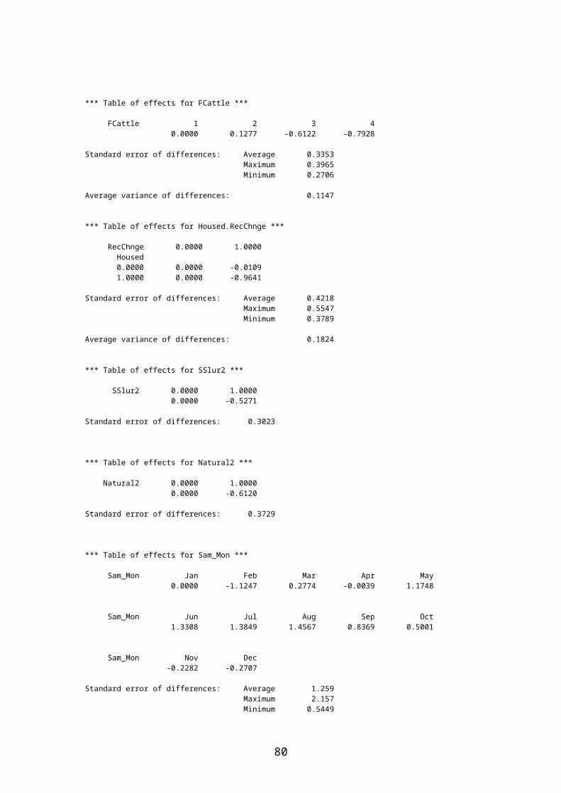
classification did in for the Binomial data. The properties of the interesting factors will therefore be reviewed in depth. These are N_F_Cattle/ FCattle/N_Groups/GroupsCat/N_Sam_Gr/Cattle/N_Cattle, Source/NewSource, Breed/ BeefonDairy (BeefonDairy is defined as a particular interaction of a management and a breed factor), Grass_Manure, Grass_Slurry, N_Goats, Pigs, LabOperator. Sample_Year and a variety of associated Sample_Month and/or Seasonal factors are all worth further investigation as possible descriptive factors. Note that the variables have been grouped, where appropriate, into equivalence classes of what are likely to be highly correlated factors.
Exploring the N_F_Cattle/FCattle/N_Groups/GroupsCat/N_Sam_Gr/Cattle/N_Cattle group, all of these measures are associated with the size of the animal population on the farm. All of these factors and variables associate higher numbers of cattle and/or groups with a higher probability of the farm exhibiting a sample containing VT E. coli O157. Examining the output from the model for N_F_Cattle, we note the high leverage which is associated with the larger values of the explanatory variable.
5621 MODEL [DISTRIBUTION=binomial; LINK=logit; DISPERSION=1] VFarmPos; NBINOMIAL=N_Bin5622 TERMS [FACT=9] N_F_Catt5623 FIT [PRINT=model,summary,estimates; CONSTANT=estimate; FPROB=yes; TPROB=yes; FACT=9]\5624 N_F_Catt ***** Regression Analysis ***** Response variate: VFarmPos Binomial totals: N_Bin Distribution: Binomial Link function: Logit Fitted terms: Constant, N_F_Catt *** Summary of analysis *** mean deviance approx d.f. deviance deviance ratio chi prRegression 1 17.1 17.065 17.06 <.001Residual 950 980.0 1.032Total 951 997.0 1.048* MESSAGE: ratios are based on dispersion parameter with value 1 Dispersion parameter is fixed at 1.00* MESSAGE: The error variance does not appear to be constant: intermediate responses are more variable than small or largeresponses* MESSAGE: The following units have high leverage: Unit Response Leverage 65 0.00 0.0606 70 1.00 0.0118 130 1.00 0.0212 172 0.00 0.0225 286 1.00 0.0212 308 1.00 0.0102 422 0.00 0.0102 440 1.00 0.0554 444 1.00 0.0368 450 0.00 0.0673 454 0.00 0.0152 455 0.00 0.0212 496 0.00 0.0212 499 0.00 0.0152 527 0.00 0.0078 529 1.00 0.0279 545 0.00 0.0085 552 0.00 0.0102 578 1.00 0.0102 683 1.00 0.0423 737 0.00 0.0102 775 0.00 0.0131
80

781 1.00 0.0082 838 1.00 0.0111 861 1.00 0.0212 874 0.00 0.0517 884 1.00 0.0102 920 0.00 0.0187 952 0.00 0.0102 *** Estimates of parameters *** antilog of estimate s.e. t(*) t pr. estimateConstant -1.567 0.108 -14.54 <.001 0.2087N_F_Catt 0.003631 0.000884 4.11 <.001 1.004
MESSAGE: s.e.s are based on dispersion parameter with value 1
Such large leverages associated with a sparse tail of the distribution of a variable are generally associated with poor models. Hence, FCattle is to be preferred as an explanatory variable. The output from this model still exhibits the same leverage issues, but these effects are confined to the largest classification class, which is of relatively little importance.
5625 "Modelling of binomial proportions. (e.g. by logits)."5626 MODEL [DISTRIBUTION=binomial; LINK=logit; DISPERSION=1] VFarmPos; NBINOMIAL=N_Bin5627 TERMS [FACT=9] FCattle5628 FIT [PRINT=model,summary,estimates; CONSTANT=estimate; FPROB=yes; TPROB=yes; FACT=9]\5629 FCattle ***** Regression Analysis ***** Response variate: VFarmPos Binomial totals: N_Bin Distribution: Binomial Link function: Logit Fitted terms: Constant, FCattle *** Summary of analysis *** mean deviance approx d.f. deviance deviance ratio chi prRegression 3 20.1 6.704 6.70 <.001Residual 948 976.9 1.030Total 951 997.0 1.048* MESSAGE: ratios are based on dispersion parameter with value 1 Dispersion parameter is fixed at 1.00* MESSAGE: The error variance does not appear to be constant: large responses are more variable than small responses* MESSAGE: The following units have high leverage: Unit Response Leverage 22 1.00 0.0158 65 0.00 0.0158 70 1.00 0.0158 97 0.00 0.0158 130 1.00 0.0158 172 0.00 0.0158 200 0.00 0.0158 280 0.00 0.0158 286 1.00 0.0158 308 1.00 0.0158 322 0.00 0.0158 324 0.00 0.0158 355 0.00 0.0158 363 0.00 0.0158 369 0.00 0.0158 383 1.00 0.0158 386 0.00 0.0158 388 0.00 0.0158 421 0.00 0.0158
81

422 0.00 0.0158 425 1.00 0.0158 440 1.00 0.0158 444 1.00 0.0158 446 1.00 0.0158 450 0.00 0.0158 454 0.00 0.0158 455 0.00 0.0158 468 0.00 0.0158 472 0.00 0.0158 489 0.00 0.0158 496 0.00 0.0158 499 0.00 0.0158 527 0.00 0.0158 529 1.00 0.0158 545 0.00 0.0158 552 0.00 0.0158 560 0.00 0.0158 578 1.00 0.0158 620 1.00 0.0158 651 1.00 0.0158 661 0.00 0.0158 667 0.00 0.0158 683 1.00 0.0158 688 1.00 0.0158 705 0.00 0.0158 725 0.00 0.0158 737 0.00 0.0158 752 0.00 0.0158 763 0.00 0.0158 775 0.00 0.0158 781 1.00 0.0158 805 0.00 0.0158 809 1.00 0.0158 838 1.00 0.0158 857 1.00 0.0158 861 1.00 0.0158 874 0.00 0.0158 884 1.00 0.0158 897 0.00 0.0158 920 0.00 0.0158 922 1.00 0.0158 945 0.00 0.0158 952 0.00 0.0158 *** Estimates of parameters *** antilog of estimate s.e. t(*) t pr. estimateConstant -1.649 0.126 -13.08 <.001 0.1923FCattle 2 0.587 0.192 3.06 0.002 1.799FCattle 3 0.588 0.214 2.75 0.006 1.800FCattle 4 1.095 0.290 3.78 <.001 2.990* MESSAGE: s.e.s are based on dispersion parameter with value 1 Parameters for factors are differences compared with the reference level: Factor Reference level FCattle 1
When the model is refitted, constrained to model only the smaller classes, the following output is generated:5630 RESTRICT FCattle;CONDITION=FCattle.LT.45631 "Modelling of binomial proportions. (e.g. by logits)."5632 MODEL [DISTRIBUTION=binomial; LINK=logit; DISPERSION=1] VFarmPos; NBINOMIAL=N_Bin5633 TERMS [FACT=9] FCattle5634 FIT [PRINT=model,summary,estimates; CONSTANT=estimate; FPROB=yes; TPROB=yes; FACT=9]\5635 FCattle
* MESSAGE: Term FCattle cannot be fully included in the model because 1 parameter is aliased with terms already in the model (FCattle 4) = 0
82

***** Regression Analysis ***** Response variate: VFarmPos Binomial totals: N_Bin Distribution: Binomial Link function: Logit Fitted terms: Constant, FCattle *** Summary of analysis *** mean deviance approx d.f. deviance deviance ratio chi prRegression 2 12.4 6.211 6.21 0.002Residual 886 894.2 1.009Total 888 906.6 1.021* MESSAGE: ratios are based on dispersion parameter with value 1 Dispersion parameter is fixed at 1.00* MESSAGE: The error variance does not appear to be constant: large responses are more variable than small responses *** Estimates of parameters *** antilog of estimate s.e. t(*) t pr. estimateConstant -1.649 0.126 -13.08 <.001 0.1923FCattle 2 0.587 0.192 3.06 0.002 1.799FCattle 3 0.588 0.214 2.75 0.006 1.800FCattle 4 0 * * * 1.000* MESSAGE: s.e.s are based on dispersion parameter with value 1 Parameters for factors are differences compared with the reference level: Factor Reference level FCattle 1
The effect is still highly significant (p=0.002). Hence, FCattle is always to be preferred over N_F_Cattle.
Similar considerations apply to N_Group, where the tail of the distribution has a strong leverage on the model:
5642 MODEL [DISTRIBUTION=binomial; LINK=logit; DISPERSION=1] VFarmPos; NBINOMIAL=N_Bin5643 TERMS [FACT=9] N_Groups5644 FIT [PRINT=model,summary,estimates; CONSTANT=estimate; FPROB=yes; TPROB=yes; FACT=9]\5645 N_Groups ***** Regression Analysis ***** Response variate: VFarmPos Binomial totals: N_Bin Distribution: Binomial Link function: Logit Fitted terms: Constant, N_Groups *** Summary of analysis *** mean deviance approx d.f. deviance deviance ratio chi prRegression 1 4.0 4.044 4.04 0.044Residual 950 993.0 1.045Total 951 997.0 1.048* MESSAGE: ratios are based on dispersion parameter with value 1 Dispersion parameter is fixed at 1.00* MESSAGE: The following units have high leverage: Unit Response Leverage
83

65 0.00 0.0461 97 0.00 0.0104 249 0.00 0.0087 293 0.00 0.0104 324 0.00 0.0123 440 1.00 0.0594 450 0.00 0.0797 454 0.00 0.0087 487 0.00 0.0072 494 0.00 0.0087 496 0.00 0.1141 527 0.00 0.0166 529 1.00 0.0123 545 0.00 0.0277 552 0.00 0.0217 748 0.00 0.0123 781 1.00 0.0123 861 1.00 0.0217 922 1.00 0.2307 945 0.00 0.0104 946 1.00 0.0087 *** Estimates of parameters *** antilog of estimate s.e. t(*) t pr. estimateConstant -1.417 0.104 -13.56 <.001 0.2426N_Groups 0.0375 0.0185 2.02 0.043 1.038* MESSAGE: s.e.s are based on dispersion parameter with value 1
Replacing N_Groups with GroupsCat gives rise to the following output:
5652 MODEL [DISTRIBUTION=binomial; LINK=logit; DISPERSION=1] VFarmPos; NBINOMIAL=N_Bin5653 TERMS [FACT=9] GroupsCat5654 FIT [PRINT=model,summary,estimates; CONSTANT=estimate; FPROB=yes; TPROB=yes; FACT=9]\5655 GroupsCat
***** Regression Analysis ***** Response variate: VFarmPos Binomial totals: N_Bin Distribution: Binomial Link function: Logit Fitted terms: Constant, GroupsCat *** Summary of analysis *** mean deviance approx d.f. deviance deviance ratio chi prRegression 3 6.7 2.230 2.23 0.082Residual 948 990.3 1.045Total 951 997.0 1.048* MESSAGE: ratios are based on dispersion parameter with value 1 Dispersion parameter is fixed at 1.00* MESSAGE: The error variance does not appear to be constant: large responses are more variable than small responses* MESSAGE: The following units have high leverage: Unit Response Leverage 50 0.00 0.0231 65 0.00 0.0231 97 0.00 0.0231 172 0.00 0.0231 249 0.00 0.0231 254 1.00 0.0231 285 0.00 0.0231 293 0.00 0.0231 324 0.00 0.0231 330 0.00 0.0231 331 0.00 0.0231 440 1.00 0.0231 450 0.00 0.0231
84

454 0.00 0.0231 459 0.00 0.0231 460 1.00 0.0231 487 0.00 0.0231 494 0.00 0.0231 496 0.00 0.0231 520 1.00 0.0231 527 0.00 0.0231 529 1.00 0.0231 545 0.00 0.0231 552 0.00 0.0231 599 1.00 0.0231 667 0.00 0.0231 688 1.00 0.0231 692 0.00 0.0231 709 0.00 0.0231 748 0.00 0.0231 761 0.00 0.0231 775 0.00 0.0231 781 1.00 0.0231 813 1.00 0.0231 839 0.00 0.0231 857 1.00 0.0231 861 1.00 0.0231 864 1.00 0.0231 901 0.00 0.0231 922 1.00 0.0231 945 0.00 0.0231 946 1.00 0.0231 952 0.00 0.0231 *** Estimates of parameters *** antilog of estimate s.e. t(*) t pr. estimateConstant -1.604 0.178 -9.03 <.001 0.2011GroupsCat 2 0.391 0.203 1.92 0.054 1.478GroupsCat 3 0.318 0.303 1.05 0.295 1.374GroupsCat 4 0.876 0.370 2.37 0.018 2.401* MESSAGE: s.e.s are based on dispersion parameter with value 1 Parameters for factors are differences compared with the reference level: Factor Reference level GroupsCat 1
On first review, this model output may appear less acceptable than the first, since the number of high leverage observations is higher. However, these observations are all of those allocated to the highest level of the group. The true suitability of the model can again be examined by constraining the model to ignore this level.
5673 RESTRICT GroupsCat;CONDITION=GroupsCat.LT.45674 "Modelling of binomial proportions. (e.g. by logits)."5675 MODEL [DISTRIBUTION=binomial; LINK=logit; DISPERSION=1] VFarmPos; NBINOMIAL=N_Bin5676 TERMS [FACT=9] GroupsCat5677 FIT [PRINT=model,summary,estimates; CONSTANT=estimate; FPROB=yes; TPROB=yes; FACT=9]\5678 GroupsCat * MESSAGE: Term GroupsCat cannot be fully included in the model because 1 parameter is aliased with terms already in the model (GroupsCat 4) = 0 ***** Regression Analysis ***** Response variate: VFarmPos Binomial totals: N_Bin Distribution: Binomial Link function: Logit Fitted terms: Constant, GroupsCat
85
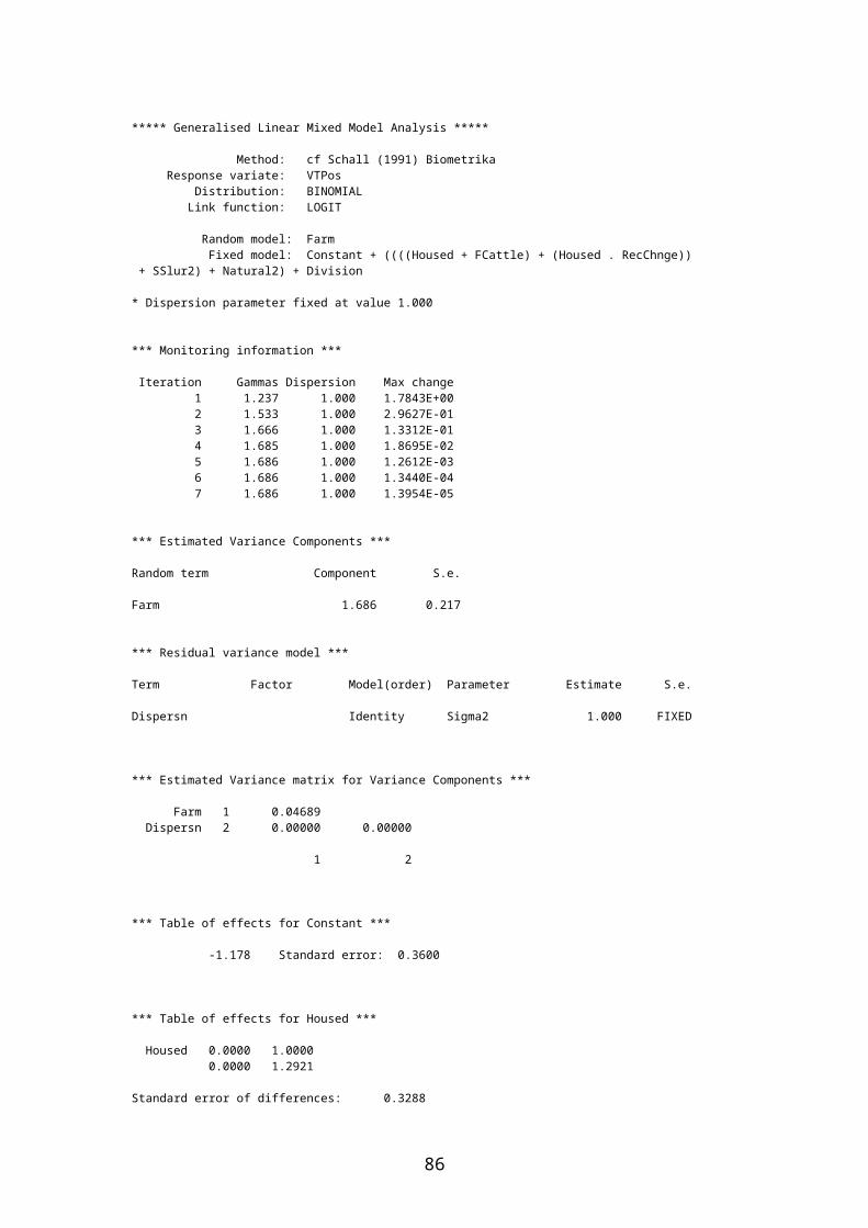
*** Summary of analysis *** mean deviance approx d.f. deviance deviance ratio chi prRegression 2 3.9 1.935 1.94 0.144Residual 906 936.1 1.033Total 908 939.9 1.035* MESSAGE: ratios are based on dispersion parameter with value 1 Dispersion parameter is fixed at 1.00* MESSAGE: The error variance does not appear to be constant: large responses are more variable than small responses *** Estimates of parameters *** antilog of estimate s.e. t(*) t pr. estimateConstant -1.604 0.178 -9.03 <.001 0.2011GroupsCat 2 0.391 0.203 1.92 0.054 1.478GroupsCat 3 0.318 0.303 1.05 0.295 1.374GroupsCat 4 0 * * * 1.000* MESSAGE: s.e.s are based on dispersion parameter with value 1 Parameters for factors are differences compared with the reference level: Factor Reference level GroupsCat 1
Leverage is not a problem in this model, but much of the significance of the effects has been lost.
5680 GROUPS [LMETHOD=*;boundaries=upper] N_Groups; RevGCat; limits=!(1.5); LABELS=!T(One, More)5681 "Modelling of binomial proportions. (e.g. by logits)."5682 MODEL [DISTRIBUTION=binomial; LINK=logit; DISPERSION=1] VFarmPos; NBINOMIAL=N_Bin5683 TERMS [FACT=9] RevGCat5684 FIT [PRINT=model,summary,estimates; CONSTANT=estimate; FPROB=yes; TPROB=yes; FACT=9]\5685 RevGCat ***** Regression Analysis ***** Response variate: VFarmPos Binomial totals: N_Bin Distribution: Binomial Link function: Logit Fitted terms: Constant, RevGCat *** Summary of analysis *** mean deviance approx d.f. deviance deviance ratio chi prRegression 1 4.6 4.581 4.58 0.032Residual 950 992.4 1.045Total 951 997.0 1.048* MESSAGE: ratios are based on dispersion parameter with value 1 Dispersion parameter is fixed at 1.00* MESSAGE: The error variance does not appear to be constant: large responses are more variable than small responses *** Estimates of parameters *** antilog of estimate s.e. t(*) t pr. estimateConstant -1.604 0.178 -9.03 <.001 0.2011RevGCat 2 0.413 0.198 2.09 0.037 1.512* MESSAGE: s.e.s are based on dispersion parameter with value 1 Parameters for factors are differences compared with the reference level: Factor Reference level
86

RevGCat 1
Hence, farms with more than one sampling group are more likely to exhibit positive samples (p=0.04). RevGCat is a more appropriate term to include in a model than N_Groups or GroupsCat.
Similar considerations apply to the N_Cattle and Cattle terms. N_Cattle is a significant variable, but some of the larger terms exert a strong leverage on the results:
5687 MODEL [DISTRIBUTION=binomial; LINK=logit; DISPERSION=1] VFarmPos; NBINOMIAL=N_Bin5688 TERMS [FACT=9] N_Cattle5689 FIT [PRINT=model,summary,estimates; CONSTANT=estimate; FPROB=yes; TPROB=yes; FACT=9]\5690 N_Cattle ***** Regression Analysis ***** Response variate: VFarmPos Binomial totals: N_Bin Distribution: Binomial Link function: Logit Fitted terms: Constant, N_Cattle *** Summary of analysis *** mean deviance approx d.f. deviance deviance ratio chi prRegression 1 8.3 8.275 8.27 0.004Residual 950 988.7 1.041Total 951 997.0 1.048* MESSAGE: ratios are based on dispersion parameter with value 1 Dispersion parameter is fixed at 1.00* MESSAGE: The following units have high leverage: Unit Response Leverage 62 1.00 0.0165 70 1.00 0.0109 182 0.00 0.0097 200 0.00 0.0104 201 0.00 0.0108 310 0.00 0.0083 370 0.00 0.0108 418 0.00 0.0072 444 1.00 0.0464 460 1.00 0.0083 494 0.00 0.0503 496 0.00 0.0216 527 0.00 0.1084 599 1.00 0.0104 651 1.00 0.0116 680 0.00 0.0125 737 0.00 0.0372 748 0.00 0.0079 750 1.00 0.0190 761 0.00 0.0417 763 0.00 0.0665 769 0.00 0.0186 884 1.00 0.0216 *** Estimates of parameters *** antilog of estimate s.e. t(*) t pr. estimateConstant -1.466 0.103 -14.18 <.001 0.2307N_Cattle 0.001299 0.000446 2.91 0.004 1.001
MESSAGE: s.e.s are based on dispersion parameter with value 1
87

Fitting Cattle gives similar results, but the leverage effects are confined to the larger two levels.5692 MODEL [DISTRIBUTION=binomial; LINK=logit; DISPERSION=1] VFarmPos; NBINOMIAL=N_Bin5693 TERMS [FACT=9] Cattle5694 FIT [PRINT=model,summary,estimates; CONSTANT=estimate; FPROB=yes; TPROB=yes; FACT=9]\5695 Cattle 5695............................................................................ ***** Regression Analysis ***** Response variate: VFarmPos Binomial totals: N_Bin Distribution: Binomial Link function: Logit Fitted terms: Constant, Cattle *** Summary of analysis *** mean deviance approx d.f. deviance deviance ratio chi prRegression 3 14.4 4.815 4.81 0.002Residual 948 982.6 1.036Total 951 997.0 1.048* MESSAGE: ratios are based on dispersion parameter with value 1 Dispersion parameter is fixed at 1.00* MESSAGE: The error variance does not appear to be constant: large responses are more variable than small responses* MESSAGE: The following units have high leverage: Unit Response Leverage 62 1.00 0.0454 70 1.00 0.0454 165 0.00 0.0454 182 0.00 0.0454 200 0.00 0.0454 201 0.00 0.0454 284 1.00 0.0454 310 0.00 0.0454 348 0.00 0.0454 370 0.00 0.0454 418 0.00 0.0454 437 0.00 0.0454 444 1.00 0.1664 460 1.00 0.0454 494 0.00 0.1664 496 0.00 0.0454 527 0.00 0.1664 599 1.00 0.0454 603 1.00 0.0454 651 1.00 0.0454 680 0.00 0.0454 737 0.00 0.1664 748 0.00 0.0454 750 1.00 0.0454 761 0.00 0.1664 763 0.00 0.1664 769 0.00 0.0454 884 1.00 0.0454 *** Estimates of parameters *** antilog of estimate s.e. t(*) t pr. estimateConstant -1.560 0.118 -13.24 <.001 0.2101Cattle 2 0.514 0.162 3.18 0.001 1.672Cattle 3 1.192 0.449 2.65 0.008 3.294Cattle 4 -0.05 1.10 -0.04 0.964 0.9517* MESSAGE: s.e.s are based on dispersion parameter with value 1 Parameters for factors are differences compared with the reference level:
88

Factor Reference level Cattle 1
However, the leverage issues are restricted to the largest two levels of the factor. Refitting the model, restricting the fit to lower levels, gives the following output:5701 RESTRICT Cattle;CONDITION=Cattle.LT.3 * MESSAGE: The structure Cattle is already restricted. Results may be unexpected.5702 MODEL [DISTRIBUTION=binomial; LINK=logit; DISPERSION=1] VFarmPos; NBINOMIAL=N_Bin5703 TERMS [FACT=9] Cattle5704 FIT [PRINT=model,summary,estimates; CONSTANT=estimate; FPROB=yes; TPROB=yes; FACT=9]\5705 Cattle
* MESSAGE: Term Cattle cannot be fully included in the model because 2 parameters are aliased with terms already in the model (Cattle 3) = 0 (Cattle 4) = 0 ***** Regression Analysis ***** Response variate: VFarmPos Binomial totals: N_Bin Distribution: Binomial Link function: Logit Fitted terms: Constant, Cattle *** Summary of analysis *** mean deviance approx d.f. deviance deviance ratio chi prRegression 1 10.2 10.176 10.18 0.001Residual 922 947.4 1.028Total 923 957.6 1.037* MESSAGE: ratios are based on dispersion parameter with value 1 Dispersion parameter is fixed at 1.00* MESSAGE: The error variance does not appear to be constant: large responses are more variable than small responses *** Estimates of parameters *** antilog of estimate s.e. t(*) t pr. estimateConstant -1.560 0.118 -13.24 <.001 0.2101Cattle 2 0.514 0.162 3.18 0.001 1.672Cattle 3 0 * * * 1.000Cattle 4 0 * * * 1.000* MESSAGE: s.e.s are based on dispersion parameter with value 1 Parameters for factors are differences compared with the reference level: Factor Reference level Cattle 1
The Cattle factor is highly significant and well-fitting. It is therefore preferable to the N_Cattle variable.
Fitting N_Sam_Gr gives rise to the following output:
5557 GROUPS [LMETHOD=*;boundaries=upper] N_Groups; RevGCat; limits=!(1.5); LABELS=!T(One, More)5558 MODEL [DISTRIBUTION=binomial; LINK=logit; DISPERSION=1] VFarmPos; NBINOMIAL=N_Bin5559 FIT [PRINT=model,summary,estimates; CONSTANT=estimate; FPROB=yes; TPROB=yes; FACT=9]\5560 N_Sam_Gr
89

5560............................................................................ ***** Regression Analysis ***** Response variate: VFarmPos Binomial totals: N_Bin Distribution: Binomial Link function: Logit Fitted terms: Constant, N_Sam_Gr *** Summary of analysis *** mean deviance approx d.f. deviance deviance ratio chi prRegression 1 23.1 23.052 23.05 <.001Residual 950 974.0 1.025Total 951 997.0 1.048* MESSAGE: ratios are based on dispersion parameter with value 1 Dispersion parameter is fixed at 1.00* MESSAGE: The following units have high leverage: Unit Response Leverage 18 0.00 0.0147 54 0.00 0.0098 59 0.00 0.0074 61 1.00 0.0070 70 1.00 0.0505 107 0.00 0.0126 123 0.00 0.0351 149 0.00 0.0158 167 0.00 0.0290 267 1.00 0.0186 363 0.00 0.0228 413 0.00 0.0169 440 1.00 0.0074 503 0.00 0.0158 510 0.00 0.0074 532 1.00 0.0169 544 0.00 0.0098 578 1.00 0.0228 584 1.00 0.0351 603 1.00 0.0090 609 0.00 0.0198 620 1.00 0.0290 637 1.00 0.0074 681 1.00 0.0136 703 1.00 0.0290 743 0.00 0.0070 781 1.00 0.0136 831 0.00 0.0141 838 1.00 0.0074 891 0.00 0.0086 906 0.00 0.0406 924 0.00 0.0116 *** Estimates of parameters *** antilog of estimate s.e. t(*) t pr. estimateConstant -1.770 0.134 -13.23 <.001 0.1703N_Sam_Gr 0.02106 0.00444 4.75 <.001 1.021* MESSAGE: s.e.s are based on dispersion parameter with value 1
Again, many of the points have a high leverage: these are farms with particularly high numbers of animals. Examining the properties of N_Sam_Gr we define a factor based on the quartiles of the distribution.
5583 DESCRIBE [SELECTION=nobs,nmv,mean,median,min,max,q1,q3] N_Sam_Gr
90
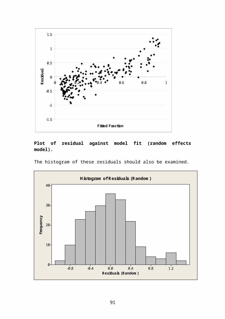
Summary statistics for N_Sam_Gr Number of observations = 952 Number of missing values = 0 Mean = 21.85 Median = 17.00 Minimum = 2.00 Maximum = 177.00 Lower quartile = 11.00 Upper quartile = 28.00
5586 GROUPS [LMETHOD=*;boundaries=upper] N_Sam_Gr; SamGrF; limits=!(11,17,28)
5586 GROUPS [LMETHOD=*;boundaries=upper] N_Sam_Gr; SamGrF; limits=!(11,17,28)5587 MODEL [DISTRIBUTION=binomial; LINK=logit; DISPERSION=1] VFarmPos; NBINOMIAL=N_Bin5588 FIT [PRINT=model,summary,estimates; CONSTANT=estimate; FPROB=yes; TPROB=yes; FACT=9]\5589 SamGrF
5589............................................................................ ***** Regression Analysis ***** Response variate: VFarmPos Binomial totals: N_Bin Distribution: Binomial Link function: Logit Fitted terms: Constant, SamGrF *** Summary of analysis *** mean deviance approx d.f. deviance deviance ratio chi prRegression 3 32.2 10.728 10.73 <.001Residual 948 964.8 1.018Total 951 997.0 1.048* MESSAGE: ratios are based on dispersion parameter with value 1 Dispersion parameter is fixed at 1.00* MESSAGE: The error variance does not appear to be constant: large responses are more variable than small responses *** Estimates of parameters *** antilog of estimate s.e. t(*) t pr. estimateConstant -2.089 0.204 -10.24 <.001 0.1239SamGrF 2 0.836 0.257 3.25 0.001 2.307SamGrF 3 0.847 0.256 3.31 <.001 2.332SamGrF 4 1.330 0.248 5.37 <.001 3.782* MESSAGE: s.e.s are based on dispersion parameter with value 1 Parameters for factors are differences compared with the reference level: Factor Reference level SamGrF 1
This factor fits well and is extremely statistically significant. Hence, SamGrF is preferred to N_Sam_Gr for further analysis.
Since Natural was such an important factor in the levels of shedding analysis, and the observed p-value in this analysis was only marginally above 0.1, it is worthwhile to review the effect of this factor in more depth. Focusing only on unhoused animals, given the negligible number of farms with housed animals and a natural source of water (7), and using the factor Natural2 to review the effect of natural water supplies on unhoused animals only, the observed p-value increases to 0.12. Hence, this factor is not considered for inclusion in the multifactor model.
91

Hence, FCattle, RevGCat, SamGrF and Cattle are the preferred factors for further review, with the other factors being removed primarily for reasons of model fit.
Exploring the FCattle/RevGCat/SamGrF/Cattle complex, which all associate higher risk of shedding being identified on a farm with larger numbers of cattle, using forward stepwise selection with the Akaike information criterion to select candidates for inclusion/exclusion, we generate the following output:
5594 MODEL [DISTRIBUTION=binomial; LINK=logit; DISPERSION=1] VFarmPos; NBINOMIAL=N_Bin5595 RSEARCH [PRINT=model,results; METHOD=fstepwise; CONSTANT=estimate; FACTORIAL=3; DENOMINATOR=ss;\5596 INRATIO=1; OUTRATIO=1; MAXCYCLE=50; AFACTORIAL=2; CRITERION=aic; EXTRA=cp; NTERMS=60;\5597 NBESTMODELS=8] FCattle+RevGCat+SamGrF+Cattle ***** Model Selection ***** Response variate: VFarmPos Binomial totals: N_Bin Distribution: Binomial Link function: Logit Number of units: 952 Forced terms: Constant Forced df: 1 Free terms: FCattle + RevGCat + SamGrF + Cattle *** Stepwise (forward) analysis of deviance *** Change mean deviance approx d.f. deviance deviance ratio chi pr+ SamGrF 3 32.184 10.728 10.73 <.001+ Cattle 3 10.905 3.635 3.63 0.012+ FCattle 3 6.721 2.240 2.24 0.081Residual 942 947.210 1.006 Total 951 997.020 1.048 Final model: Constant + SamGrF + Cattle + FCattle
The factor categorising the numbers of sampling groups is the most relevant, but the factor categorising the number of cattle on the farm also shows signs of strong statistical significance. The factor categorising the number of finishing cattle shows signs of statistical significance, even in the presence of the latter two factors. Only the factor categorising the total numbers of groups of cattle on the farm is found to lack any real statistical significance. On this basis, each of the factors FCattle, SamGrF and Cattle should be candidates for inclusion in the multivariate model.
Considering Source and NewSource as candidate factors, fitting Source (the basic data) gives the following output:
5598 MODEL [DISTRIBUTION=binomial; LINK=logit; DISPERSION=1] VFarmPos; NBINOMIAL=N_Bin5599 FIT [PRINT=model,summary,estimates; CONSTANT=estimate; FPROB=yes; TPROB=yes; FACT=9]\5600 Source ***** Regression Analysis ***** Response variate: VFarmPos Binomial totals: N_Bin Distribution: Binomial Link function: Logit Fitted terms: Constant, Source
92

*** Summary of analysis *** mean deviance approx d.f. deviance deviance ratio chi prRegression 2 4.7 2.341 2.34 0.096Residual 949 992.3 1.046Total 951 997.0 1.048* MESSAGE: ratios are based on dispersion parameter with value 1 Dispersion parameter is fixed at 1.00* MESSAGE: The error variance does not appear to be constant: large responses are more variable than small responses *** Estimates of parameters *** antilog of estimate s.e. t(*) t pr. estimateConstant -1.418 0.103 -13.73 <.001 0.2422Source Buy 0.326 0.190 1.71 0.087 1.385Source Both 0.372 0.212 1.75 0.080 1.451* MESSAGE: s.e.s are based on dispersion parameter with value 1 Parameters for factors are differences compared with the reference level: Factor Reference level Source Breed
The factor shows a moderate level of statistical significance, but this is entirely due to the differences between the class of farms which never buy replacement cattle on one hand, and those which buy or do both on the other. There is no evidence of any statistically significant difference between this latter two group: t=0.16, p=0.87. Hence, it would seem sensible to replace Source with a new factor, New Source, which consolidates the farms into a single ‘Open’ class and a ‘Closed’ class. Fitting this factor gives:
5601 MODEL [DISTRIBUTION=binomial; LINK=logit; DISPERSION=1] VFarmPos; NBINOMIAL=N_Bin5602 FIT [PRINT=model,summary,estimates; CONSTANT=estimate; FPROB=yes; TPROB=yes; FACT=9]\5603 NewSource ***** Regression Analysis ***** Response variate: VFarmPos Binomial totals: N_Bin Distribution: Binomial Link function: Logit Fitted terms: Constant, NewSource *** Summary of analysis *** mean deviance approx d.f. deviance deviance ratio chi prRegression 1 4.6 4.647 4.65 0.031Residual 950 992.4 1.045Total 951 997.0 1.048* MESSAGE: ratios are based on dispersion parameter with value 1 Dispersion parameter is fixed at 1.00* MESSAGE: The error variance does not appear to be constant: large responses are more variable than small responses *** Estimates of parameters *** antilog of estimate s.e. t(*) t pr. estimateConstant -1.418 0.103 -13.73 <.001 0.2422
93

NewSource 2 0.346 0.159 2.17 0.030 1.413* MESSAGE: s.e.s are based on dispersion parameter with value 1 Parameters for factors are differences compared with the reference level: Factor Reference level NewSource 1
Farms which never buy in replacement cattle have statistically significantly (p=0.03) lower risk of exhibiting a shedding animal than those which occasionally or frequently buy animals in. NewSource will be a candidate factor in the multivariate analysis.
BeefonDairy is a variable defined after close consideration of the properties of the dataset, in particular, Breed and Manage_O. Breed shows some evidence of significance in the bivariate analysis, but there is also evidence that the effect is confined to a subset of farms. Manage_O exhibits no evidence of significant differences in prevalence, but is important in understanding the patterns seen in Breed.
Fitting Breed as a main effect gives the following output:
5562 "Modelling of binomial proportions. (e.g. by logits)."5563 MODEL [DISTRIBUTION=binomial; LINK=logit; DISPERSION=1] VFarmPos; NBINOMIAL=N_Bin5564 TERMS [FACT=9] Breed5565 FIT [PRINT=model,summary,estimates; CONSTANT=estimate; FPROB=yes; TPROB=yes; FACT=9]\5566 Breed
5566............................................................................ * MESSAGE: Term Breed cannot be fully included in the model because 1 parameter is aliased with terms already in the model (Breed B_D) = 0 ***** Regression Analysis ***** Response variate: VFarmPos Binomial totals: N_Bin Distribution: Binomial Link function: Logit Fitted terms: Constant, Breed *** Summary of analysis *** mean deviance approx d.f. deviance deviance ratio chi prRegression 5 12.6 2.513 2.51 0.028Residual 946 984.5 1.041Total 951 997.0 1.048* MESSAGE: ratios are based on dispersion parameter with value 1 Dispersion parameter is fixed at 1.00* MESSAGE: The error variance does not appear to be constant: intermediate responses are more variable than small or largeresponses* MESSAGE: The following units have high leverage: Unit Response Leverage 7 1.00 0.091 8 0.00 0.024 17 1.00 0.091 60 0.00 0.024 87 0.00 0.024 101 1.00 0.091 110 0.00 0.024 113 0.00 0.091 116 0.00 0.091
94

118 0.00 0.091 184 0.00 0.024 185 0.00 0.091 223 0.00 0.024 280 0.00 0.024 291 0.00 0.024 306 0.00 0.024 314 0.00 0.024 338 0.00 0.024 345 0.00 0.024 350 0.00 0.024 447 0.00 0.091 479 0.00 0.024 485 0.00 0.024 494 0.00 0.024 542 0.00 0.024 593 0.00 0.024 595 0.00 0.024 596 0.00 0.024 598 0.00 0.024 599 1.00 0.024 600 0.00 0.166 607 0.00 0.024 619 0.00 0.024 620 1.00 0.166 637 1.00 0.166 645 0.00 0.024 646 1.00 0.024 661 0.00 0.024 688 1.00 0.166 702 0.00 0.024 708 0.00 0.024 725 0.00 0.024 728 0.00 0.024 729 0.00 0.024 735 0.00 0.024 747 0.00 0.024 755 0.00 0.091 762 0.00 0.024 813 1.00 0.024 825 1.00 0.024 826 0.00 0.024 856 0.00 0.024 859 1.00 0.091 864 1.00 0.024 884 1.00 0.166 896 0.00 0.024 911 0.00 0.166 951 0.00 0.024 952 0.00 0.091 *** Estimates of parameters *** antilog of estimate s.e. t(*) t pr. estimateConstant -1.2595 0.0872 -14.44 <.001 0.2838Breed DB -0.532 0.352 -1.51 0.131 0.5873Breed D 0.700 0.632 1.11 0.268 2.014Breed B_DB 0.182 0.301 0.60 0.546 1.200Breed DB_D -0.742 0.484 -1.53 0.126 0.4762Breed B_D 0 * * * 1.000Breed B_D_DB 1.953 0.868 2.25 0.024 7.047* MESSAGE: s.e.s are based on dispersion parameter with value 1 Parameters for factors are differences compared with the reference level: Factor Reference level Breed B
However, the patterns is very different on different types of farm.
Tabulating the number of farms and number of positive farms with respect to their recorded values for Breed and Manage_O, gives the following results (the number of
95

farms recorded as “Mixed” are too small for any statistical analysis, and are excluded; no animals were recorded as “B_D”):
Number Dairy Beef OtherB 11 576 173DB 59 3 8D 11 - -B_DB 25 18 18DB_D 42 - -B_D_DB 5 1 -
Positives Dairy Beef OtherB 6 123 39DB 9 0 1D 4 - -B_DB 6 6 4DB_D 5 - -B_D_DB 3 1 -
The means and marginal means for these tables are given by:
Dairy Beef Other AllB 0.545 0.214 0.225 0.221DB 0.153 0.000 0.125 0.143D 0.364 - - 0.364B_DB 0.240 0.333 0.222 0.262DB_D 0.119 - - 0.119B_D_DB 0.600 1.000 0.667All 0.216 0.217 0.221 0.218
Overall, there are clearly no significant differences between the mean prevalences on the different classes of farm. However, there is no clear evidence of any differences in the prevalence rates for different breeds on beef farms, and no evidence of any differences in the prevalence rates for different breeds on ‘Other’ farms. Similarly, for every breed except beef animals, there is no evidence of any differences in prevalence for the breed on different types of farm. However, an attempt to fit the interaction of Breed and Manage_O to the prevalence data gives the following output:
5716 "Modelling of binomial proportions. (e.g. by logits)."5717 MODEL [DISTRIBUTION=binomial; LINK=logit; DISPERSION=1] VFarmPos; NBINOMIAL=N_Bin5718 TERMS [FACT=9] Breed.Manage_O5719 FIT [PRINT=model,summary,estimates; CONSTANT=estimate; FPROB=yes; TPROB=yes; FACT=9]\5720 Breed.Manage_O 5720............................................................................ * MESSAGE: Term Breed.Manage_O cannot be fully included in the model because 14 parameters are aliased with terms already in the model (Breed B .Manage_O Mixed) = 0
96

(Breed DB .Manage_O Mixed) = 0 (Breed D .Manage_O Beef) = 0 (Breed D .Manage_O Other) = 0 (Breed D .Manage_O Mixed) = 0 (Breed DB_D .Manage_O Beef) = 0 (Breed DB_D .Manage_O Other) = 0 (Breed DB_D .Manage_O Mixed) = 0 (Breed B_D .Manage_O Dairy) = 0 (Breed B_D .Manage_O Beef) = 0 (Breed B_D .Manage_O Other) = 0 (Breed B_D .Manage_O Mixed) = 0 (Breed B_D_DB .Manage_O Other) = 0 (Breed B_D_DB .Manage_O Mixed) = 0 ***** Regression Analysis ***** Response variate: VFarmPos Binomial totals: N_Bin Distribution: Binomial Link function: Logit Fitted terms: Constant + Breed.Manage_O *** Summary of analysis *** mean deviance approx d.f. deviance deviance ratio chi prRegression 13 22.0 1.689 1.69 0.056Residual 938 975.1 1.040Total 951 997.0 1.048* MESSAGE: ratios are based on dispersion parameter with value 1 Dispersion parameter is fixed at 1.00* MESSAGE: The following units have high leverage: Unit Response Leverage 5 0.00 0.125 7 1.00 0.091 9 0.00 0.056 17 1.00 0.091 30 1.00 0.056 89 0.00 0.056 93 0.00 0.123 101 1.00 0.091 113 0.00 0.091 114 0.00 0.056 116 0.00 0.091 118 0.00 0.091 131 1.00 0.091 143 1.00 0.056 148 0.00 0.123 183 1.00 0.056 185 0.00 0.091 221 0.00 0.184 222 0.00 0.056 274 0.00 0.125 297 0.00 0.091 301 1.00 0.091 316 0.00 0.125 340 0.00 0.056 343 1.00 0.056 351 0.00 0.184 384 0.00 0.091 385 1.00 0.091 391 0.00 0.125
97

440 1.00 0.056 441 0.00 0.125 447 0.00 0.091 461 0.00 0.056 467 0.00 0.125 469 0.00 0.056 495 1.00 0.056 497 0.00 0.091 503 0.00 0.056 544 0.00 0.123 550 1.00 0.056 572 1.00 0.125 590 0.00 0.125 600 0.00 0.200 601 1.00 0.091 602 0.00 0.091 620 1.00 0.200 629 0.00 0.056 636 0.00 0.056 637 1.00 0.200 640 1.00 0.056 660 0.00 0.056 667 0.00 0.056 688 1.00 0.369 701 1.00 0.091 751 0.00 0.056 755 0.00 0.091 767 0.00 0.056 777 0.00 0.056 788 1.00 0.091 806 0.00 0.056 809 1.00 0.056 810 0.00 0.056 812 0.00 0.056 816 0.00 0.056 835 0.00 0.056 858 0.00 0.091 859 1.00 0.091 866 0.00 0.056 867 1.00 0.056 882 0.00 0.056 884 1.00 0.200 895 0.00 0.056 906 0.00 0.056 911 0.00 0.200 912 0.00 0.056 923 0.00 0.056 952 0.00 0.091 *** Estimates of parameters *** antilog of estimate s.e. t(*) t pr. estimateConstant 0.182 0.606 0.30 0.763 1.200Breed B .Manage_O Beef -1.486 0.614 -2.42 0.016 0.2263Breed B .Manage_O Other -1.417 0.632 -2.24 0.025 0.2425Breed B .Manage_O Mixed 0 * * * 1.000Breed DB .Manage_O Dairy -1.897 0.706 -2.69 0.007 0.1500Breed DB .Manage_O Beef -6.75 9.36 -0.72 0.471 0.001175Breed DB .Manage_O Other -2.13 1.23 -1.73 0.083 0.1190Breed DB .Manage_O Mixed 0 * * * 1.000Breed D .Manage_O Dairy -0.742 0.872 -0.85 0.395 0.4762Breed D .Manage_O Beef 0 * * * 1.000Breed D .Manage_O Other 0 * * * 1.000Breed D .Manage_O Mixed 0 * * * 1.000Breed B_DB .Manage_O Dairy -1.335 0.765 -1.74 0.081 0.2632Breed B_DB .Manage_O Beef -0.875 0.785 -1.11 0.265 0.4167Breed B_DB .Manage_O Other -1.435 0.830 -1.73 0.084 0.2381Breed B_DB .Manage_O Mixed -6.7 11.5 -0.59 0.556 0.001175Breed DB_D .Manage_O Dairy -2.184 0.771 -2.83 0.005 0.1126Breed DB_D .Manage_O Beef 0 * * * 1.000Breed DB_D .Manage_O Other
98

0 * * * 1.000Breed DB_D .Manage_O Mixed 0 * * * 1.000Breed B_D .Manage_O Dairy 0 * * * 1.000Breed B_D .Manage_O Beef 0 * * * 1.000Breed B_D .Manage_O Other 0 * * * 1.000Breed B_D .Manage_O Mixed 0 * * * 1.000Breed B_D_DB .Manage_O Dairy 0.22 1.10 0.20 0.839 1.250Breed B_D_DB .Manage_O Beef 5.04 8.33 0.60 0.545 153.9Breed B_D_DB .Manage_O Other 0 * * * 1.000Breed B_D_DB .Manage_O Mixed 0 * * * 1.000* MESSAGE: s.e.s are based on dispersion parameter with value 1
The model fit is extremely messy: many of the terms are aliased, and the leverage situation is extremely complicated. The model fit has a p-value of 0.056, not quite formally significant, but rather impressive where 13 degrees of freedom have been used to fit interaction terms where we believe that only one term is likely to be significant.
As noted earlier, there is no evidence of any pattern as a function of breed in the beef and ‘Other’ herds: hence it might be informative to examine the output from fitting Breed to only the Dairy herds:
5569 MODEL [DISTRIBUTION=binomial; LINK=logit; DISPERSION=1] VFarmPos; NBINOMIAL=N_Bin5570 TERMS [FACT=9] Breed5571 FIT [PRINT=model,summary,estimates; CONSTANT=estimate; FPROB=yes; TPROB=yes; FACT=9]\5572 Breed 5572............................................................................ * MESSAGE: Term Breed cannot be fully included in the model because 1 parameter is aliased with terms already in the model (Breed B_D) = 0 ***** Regression Analysis ***** Response variate: VFarmPos Binomial totals: N_Bin Distribution: Binomial Link function: Logit Fitted terms: Constant, Breed *** Summary of analysis *** mean deviance approx d.f. deviance deviance ratio chi prRegression 5 14.6 2.9249 2.92 0.012Residual 147 144.9 0.9859Total 152 159.5 1.0496* MESSAGE: ratios are based on dispersion parameter with value 1 Dispersion parameter is fixed at 1.00* MESSAGE: The error variance does not appear to be constant: large responses are more variable than small responses* MESSAGE: The following units have high leverage: Unit Response Leverage 600 0.00 0.199 620 1.00 0.199 637 1.00 0.199 884 1.00 0.199 911 0.00 0.199
99

*** Estimates of parameters *** antilog of estimate s.e. t(*) t pr. estimateConstant 0.182 0.605 0.30 0.763 1.200Breed DB -1.897 0.705 -2.69 0.007 0.1500Breed D -0.742 0.870 -0.85 0.394 0.4762Breed B_DB -1.335 0.764 -1.75 0.081 0.2632Breed DB_D -2.184 0.770 -2.84 0.005 0.1126Breed B_D 0 * * * 1.000Breed B_D_DB 0.22 1.09 0.20 0.838 1.250* MESSAGE: s.e.s are based on dispersion parameter with value 1 Parameters for factors are differences compared with the reference level: Factor Reference level Breed B
The resulting model is statistically significant (p=0.01). It may be informative to examine confidence intervals for the mean prevalences for different breeds in dairy herds:
0
0.1
0.2
0.3
0.4
0.5
0.6
0.7
0.8
0.9
1
B DB D B_D DB_D B_D_DB
Breed of Animal
Mea
n Pr
eval
ence
Restricting attention only to animals outwith the B or B_D_DB classes, the following output is generated:
5654 MODEL [DISTRIBUTION=binomial; LINK=logit; DISPERSION=1] VFarmPos; NBINOMIAL=N_Bin5655 TERMS [FACT=9] Breed5656 FIT [PRINT=model,summary,estimates; CONSTANT=estimate; FPROB=yes; TPROB=yes; FACT=9]\5657 Breed
5657............................................................................ * MESSAGE: Term Breed cannot be fully included in the model because 3 parameters are aliased with terms already in the model (Breed B) = 0 (Breed B_D) = 0 (Breed B_D_DB) = 0
100

***** Regression Analysis ***** Response variate: VFarmPos Binomial totals: N_Bin Distribution: Binomial Link function: Logit Fitted terms: Constant, Breed *** Summary of analysis *** mean deviance approx d.f. deviance deviance ratio chi prRegression 3 4.1 1.3683 1.37 0.250Residual 133 123.0 0.9251Total 136 127.1 0.9348* MESSAGE: ratios are based on dispersion parameter with value 1 Dispersion parameter is fixed at 1.00* MESSAGE: The error variance does not appear to be constant: large responses are more variable than small responses* MESSAGE: The following units have high leverage: Unit Response Leverage 7 1.00 0.091 17 1.00 0.091 101 1.00 0.091 113 0.00 0.091 116 0.00 0.091 118 0.00 0.091 185 0.00 0.091 447 0.00 0.091 755 0.00 0.091 859 1.00 0.091 952 0.00 0.091 *** Estimates of parameters *** antilog of estimate s.e. t(*) t pr. estimateConstant -1.715 0.362 -4.74 <.001 0.1800Breed B 0 * * * 1.000Breed D 1.155 0.723 1.60 0.110 3.175Breed B_DB 0.562 0.591 0.95 0.341 1.754Breed DB_D -0.287 0.598 -0.48 0.632 0.7508Breed B_D 0 * * * 1.000Breed B_D_DB 0 * * * 1.000* MESSAGE: s.e.s are based on dispersion parameter with value 1 Parameters for factors are differences compared with the reference level: Factor Reference level Breed DB
There is no evidence of any differences between the prevalences on these classes of farms. Examining the B and B_D_DB classes, tabulating their positive and negative values and carrying out a Fisher’s Exact test, we get:
5634 FEXACT2X2 [PRINT=prob] C1 ***** Fisher's Exact Test ***** One-tailed significance level 0.635 Mid-P value 0.433 Two-tailed significance level Two times one-tailed significance level 1.269 Mid-P value 0.865 Sum of all outcomes with Prob<=Observed 1.000 Mid-P value 0.798
There is no evidence of any difference in prevalence between the B and B_D_DB classes in dairy herds. However, fitting a model only to dairy herds, while excluding the beef class, gives the following output:
101

5660 MODEL [DISTRIBUTION=binomial; LINK=logit; DISPERSION=1] VFarmPos; NBINOMIAL=N_Bin5661 TERMS [FACT=9] Breed5662 FIT [PRINT=model,summary,estimates; CONSTANT=estimate; FPROB=yes; TPROB=yes; FACT=9]\5663 Breed5663............................................................................ * MESSAGE: Term Breed cannot be fully included in the model because 2 parameters are aliased with terms already in the model (Breed B) = 0 (Breed B_D) = 0 ***** Regression Analysis ***** Response variate: VFarmPos Binomial totals: N_Bin Distribution: Binomial Link function: Logit Fitted terms: Constant, Breed *** Summary of analysis *** mean deviance approx d.f. deviance deviance ratio chi prRegression 4 8.4 2.0954 2.10 0.079Residual 137 129.8 0.9472Total 141 138.1 0.9798* MESSAGE: ratios are based on dispersion parameter with value 1 Dispersion parameter is fixed at 1.00* MESSAGE: The error variance does not appear to be constant: large responses are more variable than small responses* MESSAGE: The following units have high leverage: Unit Response Leverage 600 0.00 0.199 620 1.00 0.199 637 1.00 0.199 884 1.00 0.199 911 0.00 0.199 *** Estimates of parameters *** antilog of estimate s.e. t(*) t pr. estimateConstant -1.715 0.362 -4.74 <.001 0.1800Breed B 0 * * * 1.000Breed D 1.155 0.723 1.60 0.110 3.175Breed B_DB 0.562 0.591 0.95 0.341 1.754Breed DB_D -0.287 0.598 -0.48 0.632 0.7508Breed B_D 0 * * * 1.000Breed B_D_DB 2.120 0.980 2.16 0.031 8.333* MESSAGE: s.e.s are based on dispersion parameter with value 1 Parameters for factors are differences compared with the reference level: Factor Reference level Breed DB
Hence, although the prevalence in group B_D_DB is higher, strictly speaking it is not statistically significantly higher than in the lower classes (p=0.08). However, the sample size is extremely small, and the comparison will have lacked power.
The greatest danger in this exercise is to overtrawl the data. The overall effect of fitting the Manage_O by Breed interaction was close to formal statistical significance. Hence, we are not unjustified, invoking the overall test as a type of Fisher test for multiple comparisons, in investigating the properties of individual interaction terms.
102

However, it would seem unwise to be overly liberal in then assigning importance to extremely small samples from the data, which actually lack formal statistical significance. In addition, the effect of beef animals on dairy herds appears to be specific to this type of farm. It is impossible to have the same confidence about the properties of the B_D_DB class, since the sample size in anything but the dairy herd is negligible.
In conclusion, it seems rational to create a new variable, BeefonDairy, to identify those farms with beef animals and a dairy management system. Fitting this variable gives the following results:
5665 "Modelling of binomial proportions. (e.g. by logits)."5666 MODEL [DISTRIBUTION=binomial; LINK=logit; DISPERSION=1] VFarmPos; NBINOMIAL=N_Bin5667 TERMS [FACT=9] BeefonDairy5668 FIT [PRINT=model,summary,estimates; CONSTANT=estimate; FPROB=yes; TPROB=yes; FACT=9]\5669 BeefonDairy 5669............................................................................ ***** Regression Analysis ***** Response variate: VFarmPos Binomial totals: N_Bin Distribution: Binomial Link function: Logit Fitted terms: Constant, BeefonDairy *** Summary of analysis *** mean deviance approx d.f. deviance deviance ratio chi prRegression 1 5.7 5.685 5.69 0.017Residual 950 991.3 1.044Total 951 997.0 1.048* MESSAGE: ratios are based on dispersion parameter with value 1 Dispersion parameter is fixed at 1.00* MESSAGE: The error variance does not appear to be constant: large responses are more variable than small responses* MESSAGE: The following units have high leverage: Unit Response Leverage 131 1.00 0.0908 297 0.00 0.0908 301 1.00 0.0908 384 0.00 0.0908 385 1.00 0.0908 497 0.00 0.0908 601 1.00 0.0908 602 0.00 0.0908 701 1.00 0.0908 788 1.00 0.0908 858 0.00 0.0908 *** Estimates of parameters *** antilog of estimate s.e. t(*) t pr. estimateConstant -1.3033 0.0794 -16.42 <.001 0.2716BeefonDairy 1 1.486 0.610 2.43 0.015 4.418* MESSAGE: s.e.s are based on dispersion parameter with value 1 Parameters for factors are differences compared with the reference level: Factor Reference level BeefonDairy 0
103

Farms in this class appear to have a significantly (p=0.02) higher prevalence. However, care must be taken over interpreting this factor, since it is derived from an extensive examination of the properties of the dataset. However, BeefonDairy should clearly be incorporated into the multivariate analysis. Fitting a model with both BeefonDairy and Breed as main effects, we generate the following output:
5679 MODEL [DISTRIBUTION=binomial; LINK=logit; DISPERSION=1] VFarmPos; NBINOMIAL=N_Bin5680 TERMS [FACT=9] BeefonDairy+Breed5681 FIT [PRINT=model,summary,estimates; CONSTANT=estimate; FPROB=yes; TPROB=yes; FACT=9]\5682 BeefonDairy+Breed 5682............................................................................ * MESSAGE: Term Breed cannot be fully included in the model because 1 parameter is aliased with terms already in the model (Breed B_D) = 0 ***** Regression Analysis ***** Response variate: VFarmPos Binomial totals: N_Bin Distribution: Binomial Link function: Logit Fitted terms: Constant + BeefonDairy + Breed *** Summary of analysis *** mean deviance approx d.f. deviance deviance ratio chi prRegression 6 18.1 3.019 3.02 0.006Residual 945 978.9 1.036Total 951 997.0 1.048* MESSAGE: ratios are based on dispersion parameter with value 1 Dispersion parameter is fixed at 1.00* MESSAGE: The error variance does not appear to be constant: large responses are more variable than small responses* MESSAGE: The following units have high leverage: Unit Response Leverage 7 1.00 0.091 17 1.00 0.091 101 1.00 0.091 113 0.00 0.091 116 0.00 0.091 118 0.00 0.091 131 1.00 0.091 185 0.00 0.091 297 0.00 0.091 301 1.00 0.091 384 0.00 0.091 385 1.00 0.091 447 0.00 0.091 497 0.00 0.091 600 0.00 0.166 601 1.00 0.091 602 0.00 0.091 620 1.00 0.166 637 1.00 0.166 688 1.00 0.166 701 1.00 0.091 755 0.00 0.091 788 1.00 0.091 858 0.00 0.091 859 1.00 0.091 884 1.00 0.166 911 0.00 0.166 952 0.00 0.091
104

*** Estimates of parameters *** antilog of estimate s.e. t(*) t pr. estimateConstant -1.792 0.341 -5.25 <.001 0.1667BeefonDairy 1 1.470 0.611 2.40 0.016 4.348Breed B 0.504 0.353 1.43 0.153 1.656Breed D 1.232 0.713 1.73 0.084 3.429Breed B_DB 0.714 0.447 1.60 0.110 2.043Breed DB_D -0.210 0.586 -0.36 0.721 0.8108Breed B_D 0 * * * 1.000Breed B_D_DB 2.485 0.928 2.68 0.007 12.00* MESSAGE: s.e.s are based on dispersion parameter with value 1 Parameters for factors are differences compared with the reference level: Factor Reference level BeefonDairy 0 Breed DB 5683 DROP [PRINT=model,summary,estimates; CONSTANT=estimate; FPROB=yes; TPROB=yes] Breed 5683............................................................................ ***** Regression Analysis ***** Response variate: VFarmPos Binomial totals: N_Bin Distribution: Binomial Link function: Logit Fitted terms: Constant + BeefonDairy *** Summary of analysis *** mean deviance approx d.f. deviance deviance ratio chi prRegression 1 5.7 5.685 5.69 0.017Residual 950 991.3 1.044Total 951 997.0 1.048 Change 5 12.4 2.486 2.49 0.029* MESSAGE: ratios are based on dispersion parameter with value 1 Dispersion parameter is fixed at 1.00* MESSAGE: The error variance does not appear to be constant: large responses are more variable than small responses* MESSAGE: The following units have high leverage: Unit Response Leverage 131 1.00 0.0908 297 0.00 0.0908 301 1.00 0.0908 384 0.00 0.0908 385 1.00 0.0908 497 0.00 0.0908 601 1.00 0.0908 602 0.00 0.0908 701 1.00 0.0908 788 1.00 0.0908 858 0.00 0.0908 *** Estimates of parameters *** antilog of estimate s.e. t(*) t pr. estimateConstant -1.3033 0.0794 -16.42 <.001 0.2716BeefonDairy 1 1.486 0.610 2.43 0.015 4.418* MESSAGE: s.e.s are based on dispersion parameter with value 1 Parameters for factors are differences compared with the reference level: Factor Reference level BeefonDairy 0
105
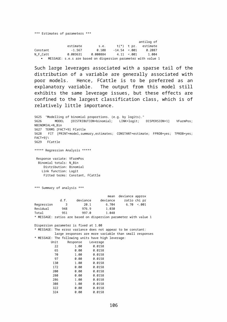
Both Breed (p=0.03) and BeefonDairy (p=0.02) are formally significantly explaining variability in the dataset. The latter is no surprise, but the former result deserves further attention. It is no surprise that the effect is completely driven by the B_D_DB level of the factor. This small group of 6 farms have a much higher prevalence. Leverage is a problem, but it would seem reasonable to define a new factor based exclusively around this breed, and include it in the multivariate analysis. Fitting Breed2 gives the following output:
5722 MODEL [DISTRIBUTION=binomial; LINK=logit; DISPERSION=1] VFarmPos; NBINOMIAL=N_Bin5723 TERMS [FACT=9] Breed25724 FIT [PRINT=model,summary,estimates; CONSTANT=estimate; FPROB=yes; TPROB=yes; FACT=9]\5725 Breed2
5725............................................................................ ***** Regression Analysis ***** Response variate: VFarmPos Binomial totals: N_Bin Distribution: Binomial Link function: Logit Fitted terms: Constant, Breed2 *** Summary of analysis *** mean deviance approx d.f. deviance deviance ratio chi prRegression 1 5.6 5.595 5.59 0.018Residual 950 991.4 1.044Total 951 997.0 1.048* MESSAGE: ratios are based on dispersion parameter with value 1 Dispersion parameter is fixed at 1.00* MESSAGE: The following units have high leverage: Unit Response Leverage 600 0.00 0.1656 620 1.00 0.1656 637 1.00 0.1656 688 1.00 0.1656 884 1.00 0.1656 911 0.00 0.1656 *** Estimates of parameters *** antilog of estimate s.e. t(*) t pr. estimateConstant -1.2975 0.0790 -16.42 <.001 0.2732Breed2 1 1.991 0.867 2.30 0.022 7.320* MESSAGE: s.e.s are based on dispersion parameter with value 1 Parameters for factors are differences compared with the reference level: Factor Reference level Breed2 0
Breed2 is therefore included in the multivariate analysis.
When investigating the properties of the factors Grass_Manure and Grass_Slurry, it is important to remember that these questions were, for the most part, only asked of farms where the animals were at pasture. Only 3 farms with housed animals recorded an answer to the questions about the properties of their pasture.
Tabulating out the properties by Housing and slurry status gives the following tables:
106

Number of FarmsHoused No Slurry Yes SlurryBlank
0 308 77 01 3 0 563
Number PositiveHoused No Slurry Yes SlurryBlank
0 53 27 -1 0 - 126
Fraction PositiveHoused No Slurry Yes SlurryBlank
0 0.172 0.351 -1 0.000 - 0.224
The effect is clearly not just due to differences between housed and unhoused farms. Fitting the GLM gives the following output (the effect of the small number of housed animals which have non blank returns will be small and hence will be ignored for the moment):
5789 MODEL [DISTRIBUTION=binomial; LINK=logit; DISPERSION=1] VFarmPos; NBINOMIAL=N_Bin5790 TERMS [FACT=9] Gra_Slur5791 FIT [PRINT=model,summary,estimates; CONSTANT=estimate; FPROB=yes; TPROB=yes; FACT=9]\5792 Gra_Slur 5792............................................................................ ***** Regression Analysis ***** Response variate: VFarmPos Binomial totals: N_Bin Distribution: Binomial Link function: Logit Fitted terms: Constant, Gra_Slur *** Summary of analysis *** mean deviance approx d.f. deviance deviance ratio chi prRegression 2 11.6 5.777 5.78 0.003Residual 948 982.4 1.036Total 950 994.0 1.046* MESSAGE: ratios are based on dispersion parameter with value 1 Dispersion parameter is fixed at 1.00* MESSAGE: The error variance does not appear to be constant: large responses are more variable than small responses* MESSAGE: The following units have high leverage: Unit Response Leverage 46 0.00 0.0129 51 1.00 0.0129 53 1.00 0.0129 55 1.00 0.0129 61 1.00 0.0129 63 0.00 0.0129 80 1.00 0.0129 83 0.00 0.0129 84 0.00 0.0129 86 0.00 0.0129 87 0.00 0.0129 92 0.00 0.0129
107

100 1.00 0.0129 110 0.00 0.0129 116 0.00 0.0129 118 0.00 0.0129 119 0.00 0.0129 128 0.00 0.0129 129 0.00 0.0129 132 0.00 0.0129 133 1.00 0.0129 135 0.00 0.0129 139 1.00 0.0129 143 1.00 0.0129 174 1.00 0.0129 180 0.00 0.0129 189 1.00 0.0129 190 0.00 0.0129 196 1.00 0.0129 199 0.00 0.0129 202 1.00 0.0129 204 1.00 0.0129 206 0.00 0.0129 215 1.00 0.0129 217 1.00 0.0129 219 0.00 0.0129 225 0.00 0.0129 226 0.00 0.0129 230 0.00 0.0129 247 0.00 0.0129 345 0.00 0.0129 507 0.00 0.0129 533 0.00 0.0129 541 0.00 0.0129 542 0.00 0.0129 543 0.00 0.0129 546 0.00 0.0129 547 0.00 0.0129 548 0.00 0.0129 552 0.00 0.0129 566 1.00 0.0129 578 1.00 0.0129 581 1.00 0.0129 593 0.00 0.0129 598 0.00 0.0129 603 1.00 0.0129 606 0.00 0.0129 608 0.00 0.0129 612 0.00 0.0129 613 1.00 0.0129 637 1.00 0.0129 639 1.00 0.0129 640 1.00 0.0129 645 0.00 0.0129 646 1.00 0.0129 659 0.00 0.0129 662 0.00 0.0129 663 0.00 0.0129 665 0.00 0.0129 670 0.00 0.0129 677 0.00 0.0129 681 1.00 0.0129 690 0.00 0.0129 702 0.00 0.0129 703 1.00 0.0129 707 0.00 0.0129 924 0.00 0.0129 *** Estimates of parameters *** antilog of estimate s.e. t(*) t pr. estimateConstant -1.583 0.151 -10.50 <.001 0.2054Gra_Slur 1 0.967 0.282 3.43 <.001 2.629Gra_Slur 999 0.339 0.181 1.87 0.061 1.404* MESSAGE: s.e.s are based on dispersion parameter with value 1 Parameters for factors are differences compared with the reference level:
108

Factor Reference level Gra_Slur 0
Among animals at pasture, those on farms which spread slurry on the grass are at a higher risk of presenting shedding than those on farms which do not.
Considering Gra_Manure, we can generate the following tables:
Number of FarmsHoused No Manure Yes Manure Blank
0 281 104 01 3 0 563
Number PositiveHoused No Manure Yes Manure Blank
0 67 13 1 0 126
Fraction PositiveHoused No Manure Yes Manure Blank
0 0.238 0.125 1 0.000 0.224
Again, any significance due to this factor is clearly not just due to differences between housed and unhoused animals. In fact, the prevalences in housed and unhoused/with no manure on pasture farms are virtually identical. The apparent effect is of unhoused farms which do spread manure having a lower prevalence. Fitting this as a GLM gives the following output:
5801 MODEL [DISTRIBUTION=binomial; LINK=logit; DISPERSION=1] VFarmPos; NBINOMIAL=N_Bin5802 TERMS [FACT=9] Gra_Manu5803 FIT [PRINT=model,summary,estimates; CONSTANT=estimate; FPROB=yes; TPROB=yes; FACT=9]\5804 Gra_Manu 5804............................................................................ ***** Regression Analysis ***** Response variate: VFarmPos Binomial totals: N_Bin Distribution: Binomial Link function: Logit Fitted terms: Constant, Gra_Manu *** Summary of analysis *** mean deviance approx d.f. deviance deviance ratio chi prRegression 2 6.6 3.307 3.31 0.037Residual 948 987.3 1.042Total 950 994.0 1.046* MESSAGE: ratios are based on dispersion parameter with value 1 Dispersion parameter is fixed at 1.00* MESSAGE: The error variance does not appear to be constant: large responses are more variable than small responses
109

*** Estimates of parameters *** antilog of estimate s.e. t(*) t pr. estimateConstant -1.175 0.139 -8.43 <.001 0.3088Gra_Manu 1 -0.771 0.328 -2.35 0.019 0.4627Gra_Manu 999 -0.068 0.172 -0.40 0.691 0.9338* MESSAGE: s.e.s are based on dispersion parameter with value 1 Parameters for factors are differences compared with the reference level: Factor Reference level Gra_Manu 0
As indicated above, the significant effect (p=0.04) is associated with the spreading of manure on farms with unhoused animals, where farms which spread manure are less likely to present shedding animals.
It is necessary to investigate whether there is any confounding of effects occurring between Gra_Slurry and Gra_Manure. Tabulating out the properties of the datset gives the following tables:
Number of Farms
Unhoused Slurry Manure 0 1
0 241 401 67 37
Housed 563
Number Positive
Unhoused Slurry Manure 0 1
0 49 181 4 9
Housed 126
Fraction Positive
Unhoused Slurry Manure 0 1
0 0.203 0.4501 0.060 0.243
Housed 0.224
All the groups have reasonable support in the data, and it is clear that the Slurry and Manure effects both appear to be operating on unhoused animals. Fitting both terms in the same GLM gives the following results (aliasing, mainly due to the blank coding in both factors for most housed farms makes the output messy, but will not affect the main estimates of interest):
110

5815 MODEL [DISTRIBUTION=binomial; LINK=logit; DISPERSION=1] VFarmPos; NBINOMIAL=N_Bin5816 TERMS [FACT=9] Gra_Manu*Gra_Slur5817 FIT [PRINT=model,summary,estimates; CONSTANT=estimate; FPROB=yes; TPROB=yes; FACT=9]\5818 Gra_Manu*Gra_Slur 5818............................................................................ * MESSAGE: Term Gra_Slur cannot be fully included in the model because 1 parameter is aliased with terms already in the model (Gra_Slur 999) = (Gra_Manu 999) * MESSAGE: Term Gra_Manu.Gra_Slur cannot be fully included in the model because 3 parameters are aliased with terms already in the model (Gra_Manu 1 .Gra_Slur 999) = 0 (Gra_Manu 999 .Gra_Slur 1) = 0 (Gra_Manu 999 .Gra_Slur 999) = (Gra_Manu 999) ***** Regression Analysis ***** Response variate: VFarmPos Binomial totals: N_Bin Distribution: Binomial Link function: Logit Fitted terms: Constant + Gra_Manu + Gra_Slur + Gra_Manu.Gra_Slur *** Summary of analysis *** mean deviance approx d.f. deviance deviance ratio chi prRegression 4 24.1 6.034 6.03 <.001Residual 946 969.8 1.025Total 950 994.0 1.046* MESSAGE: ratios are based on dispersion parameter with value 1 Dispersion parameter is fixed at 1.00* MESSAGE: The residuals do not appear to be random; for example, fitted values in the range 0.22 to 0.22 are consistently larger than observed values and fitted values in the range 0.45 to 0.45 are consistently smaller than observed values* MESSAGE: The error variance does not appear to be constant: large responses are more variable than small responses* MESSAGE: The following units have high leverage: Unit Response Leverage 46 0.00 0.0269 51 1.00 0.0250 53 1.00 0.0250 55 1.00 0.0250 61 1.00 0.0269 63 0.00 0.0250 80 1.00 0.0269 83 0.00 0.0250 84 0.00 0.0269 86 0.00 0.0269 87 0.00 0.0250 92 0.00 0.0269 100 1.00 0.0250 110 0.00 0.0250 116 0.00 0.0269 118 0.00 0.0269 119 0.00 0.0269 128 0.00 0.0250 129 0.00 0.0269 132 0.00 0.0269 133 1.00 0.0250 135 0.00 0.0250 139 1.00 0.0269 143 1.00 0.0250 174 1.00 0.0269
111

180 0.00 0.0269 189 1.00 0.0250 190 0.00 0.0269 196 1.00 0.0269 199 0.00 0.0269 202 1.00 0.0250 204 1.00 0.0250 206 0.00 0.0269 215 1.00 0.0250 217 1.00 0.0250 219 0.00 0.0269 225 0.00 0.0269 226 0.00 0.0250 230 0.00 0.0250 247 0.00 0.0250 345 0.00 0.0250 507 0.00 0.0269 533 0.00 0.0250 541 0.00 0.0269 542 0.00 0.0250 543 0.00 0.0250 546 0.00 0.0250 547 0.00 0.0250 548 0.00 0.0250 552 0.00 0.0269 566 1.00 0.0250 578 1.00 0.0250 581 1.00 0.0269 593 0.00 0.0250 598 0.00 0.0250 603 1.00 0.0269 606 0.00 0.0269 608 0.00 0.0250 612 0.00 0.0250 613 1.00 0.0250 637 1.00 0.0269 639 1.00 0.0250 640 1.00 0.0269 645 0.00 0.0269 646 1.00 0.0250 659 0.00 0.0250 662 0.00 0.0269 663 0.00 0.0269 665 0.00 0.0269 670 0.00 0.0269 677 0.00 0.0269 681 1.00 0.0250 690 0.00 0.0250 702 0.00 0.0269 703 1.00 0.0250 707 0.00 0.0269 924 0.00 0.0269 *** Estimates of parameters *** antilog of estimate s.e. t(*) t pr. estimateConstant -1.381 0.159 -8.66 <.001 0.2513Gra_Manu 1 -1.376 0.539 -2.55 0.011 0.2527Gra_Manu 999 0.138 0.189 0.73 0.466 1.147Gra_Slur 1 1.180 0.356 3.32 <.001 3.256Gra_Slur 999 0 * * * 1.000Gra_Manu 1 .Gra_Slur 1 0.441 0.733 0.60 0.547 1.555Gra_Manu 1 .Gra_Slur 999 0 * * * 1.000Gra_Manu 999 .Gra_Slur 1 0 * * * 1.000Gra_Manu 999 .Gra_Slur 999 0 * * * 1.000* MESSAGE: s.e.s are based on dispersion parameter with value 1 Parameters for factors are differences compared with the reference level: Factor Reference level Gra_Manu 0 Gra_Slur 0 5819 DROP [PRINT=model,summary,estimates; CONSTANT=estimate; FPROB=yes; TPROB=yes] Gra_Manu.Gra_Slur
112

5819............................................................................ * MESSAGE: Term Gra_Slur cannot be fully included in the model because 1 parameter is aliased with terms already in the model (Gra_Slur 999) = (Gra_Manu 999) ***** Regression Analysis ***** Response variate: VFarmPos Binomial totals: N_Bin Distribution: Binomial Link function: Logit Fitted terms: Constant + Gra_Manu + Gra_Slur *** Summary of analysis *** mean deviance approx d.f. deviance deviance ratio chi prRegression 3 23.8 7.922 7.92 <.001Residual 947 970.2 1.024Total 950 994.0 1.046 Change 1 0.4 0.370 0.37 0.543* MESSAGE: ratios are based on dispersion parameter with value 1 Dispersion parameter is fixed at 1.00* MESSAGE: The residuals do not appear to be random; for example, fitted values in the range 0.22 to 0.22 are consistently larger than observed values and fitted values in the range 0.47 to 0.47 are consistently smaller than observed values* MESSAGE: The error variance does not appear to be constant: large responses are more variable than small responses* MESSAGE: The following units have high leverage: Unit Response Leverage 46 0.00 0.0185 51 1.00 0.0200 53 1.00 0.0200 55 1.00 0.0200 61 1.00 0.0185 63 0.00 0.0200 80 1.00 0.0185 83 0.00 0.0200 84 0.00 0.0185 86 0.00 0.0185 87 0.00 0.0200 92 0.00 0.0185 100 1.00 0.0200 110 0.00 0.0200 116 0.00 0.0185 118 0.00 0.0185 119 0.00 0.0185 128 0.00 0.0200 129 0.00 0.0185 132 0.00 0.0185 133 1.00 0.0200 135 0.00 0.0200 139 1.00 0.0185 143 1.00 0.0200 174 1.00 0.0185 180 0.00 0.0185 189 1.00 0.0200 190 0.00 0.0185 196 1.00 0.0185 199 0.00 0.0185 202 1.00 0.0200 204 1.00 0.0200 206 0.00 0.0185 215 1.00 0.0200 217 1.00 0.0200 219 0.00 0.0185 225 0.00 0.0185 226 0.00 0.0200
113

230 0.00 0.0200 247 0.00 0.0200 345 0.00 0.0200 507 0.00 0.0185 533 0.00 0.0200 541 0.00 0.0185 542 0.00 0.0200 543 0.00 0.0200 546 0.00 0.0200 547 0.00 0.0200 548 0.00 0.0200 552 0.00 0.0185 566 1.00 0.0200 578 1.00 0.0200 581 1.00 0.0185 593 0.00 0.0200 598 0.00 0.0200 603 1.00 0.0185 606 0.00 0.0185 608 0.00 0.0200 612 0.00 0.0200 613 1.00 0.0200 637 1.00 0.0185 639 1.00 0.0200 640 1.00 0.0185 645 0.00 0.0185 646 1.00 0.0200 659 0.00 0.0200 662 0.00 0.0185 663 0.00 0.0185 665 0.00 0.0185 670 0.00 0.0185 677 0.00 0.0185 681 1.00 0.0200 690 0.00 0.0200 702 0.00 0.0185 703 1.00 0.0200 707 0.00 0.0185 924 0.00 0.0185 *** Estimates of parameters *** antilog of estimate s.e. t(*) t pr. estimateConstant -1.403 0.156 -8.97 <.001 0.2459Gra_Manu 1 -1.148 0.354 -3.24 0.001 0.3172Gra_Manu 999 0.159 0.186 0.86 0.392 1.173Gra_Slur 1 1.288 0.307 4.19 <.001 3.624Gra_Slur 999 0 * * * 1.000* MESSAGE: s.e.s are based on dispersion parameter with value 1 Parameters for factors are differences compared with the reference level: Factor Reference level Gra_Manu 0 Gra_Slur 0
There is no evidence of a statistically significant interaction between the factors (p=0.54), while independently, the spreading of manure is protective and the spreading of slurry is a risk factor for shedding being observed on the farm. It will be important to stress that although this result has been established only for farms with unhoused animals, the relevant data were not collected for housed farms. Hence, both Gra_Slurry and Gra_Manure will be considered in the multifactor model.
Considering N_Goats, it is suspicious that this variable is statistically significant, while the related factor reporting the absence or presence of goats is not. Plotting a histogram of N_Goats, we see that the bulk of the records contains zero. Generating a new histogram of the non-zero values of N_Goats, we see the following picture:
114

N_Goats
Freq
uenc
y
161412108642
20
15
10
5
0
Histogram of N_Goats
Fitting the model to N_Goats, we generate the following output:
5831 MODEL [DISTRIBUTION=binomial; LINK=logit; DISPERSION=1] VFarmPos; NBINOMIAL=N_Bin5832 TERMS [FACT=9] N_Goats5833 FIT [PRINT=model,summary,estimates; CONSTANT=estimate; FPROB=yes; TPROB=yes; FACT=9]\5834 N_Goats 5834............................................................................ ***** Regression Analysis ***** Response variate: VFarmPos Binomial totals: N_Bin Distribution: Binomial Link function: Logit Fitted terms: Constant, N_Goats *** Summary of analysis *** mean deviance approx d.f. deviance deviance ratio chi prRegression 1 3.1 3.150 3.15 0.076Residual 950 993.9 1.046Total 951 997.0 1.048* MESSAGE: ratios are based on dispersion parameter with value 1 Dispersion parameter is fixed at 1.00* MESSAGE: The following units have high leverage: Unit Response Leverage 9 0.00 0.0075 95 0.00 0.0515 170 0.00 0.0075 243 0.00 0.0075 343 1.00 0.0171 366 1.00 0.0075 367 1.00 0.3600 368 0.00 0.0075 537 0.00 0.0075
115

554 0.00 0.0316 585 0.00 0.0171 673 0.00 0.0075 676 0.00 0.0515 720 1.00 0.2125 746 1.00 0.0515 766 0.00 0.0765 792 0.00 0.0075 799 0.00 0.0075 818 0.00 0.0515 *** Estimates of parameters *** antilog of estimate s.e. t(*) t pr. estimateConstant -1.2989 0.0793 -16.38 <.001 0.2728N_Goats 0.1635 0.0943 1.73 0.083 1.178
MESSAGE: s.e.s are based on dispersion parameter with value 1
The two units with the highest leverage correspond to the farms with 10 and 16 goats. Removing these ultra-high leverage points from the analysis gives rise to the following output:
5934 MODEL [DISTRIBUTION=binomial; LINK=logit; DISPERSION=1] VFarmPos; NBINOMIAL=N_Bin5935 TERMS [FACT=9] N_Goats5936 FIT [PRINT=model,summary,estimates; CONSTANT=estimate; FPROB=yes; TPROB=yes; FACT=9]\5937 N_Goats
5937............................................................................ ***** Regression Analysis ***** Response variate: VFarmPos Binomial totals: N_Bin Distribution: Binomial Link function: Logit Fitted terms: Constant, N_Goats *** Summary of analysis *** mean deviance approx d.f. deviance deviance ratio chi prRegression 1 0.0 0.019 0.02 0.891Residual 948 990.9 1.045Total 949 990.9 1.044* MESSAGE: ratios are based on dispersion parameter with value 1 Dispersion parameter is fixed at 1.00* MESSAGE: The following units have high leverage: Unit Response Leverage 9 0.00 0.0192 95 0.00 0.1143 170 0.00 0.0192 243 0.00 0.0192 343 1.00 0.0422 366 1.00 0.0192 367 0.00 0.0192 536 0.00 0.0192 553 0.00 0.0741 584 0.00 0.0422 672 0.00 0.0192 675 0.00 0.1143 744 1.00 0.1143 764 0.00 0.1626 790 0.00 0.0192 797 0.00 0.0192 816 0.00 0.1143 *** Estimates of parameters ***
116

antilog of estimate s.e. t(*) t pr. estimateConstant -1.2888 0.0795 -16.22 <.001 0.2756N_Goats -0.023 0.172 -0.14 0.892 0.9770* MESSAGE: s.e.s are based on dispersion parameter with value 1
Having removed the two high leverage points, N_Goats no longer exhibits any particular statistical significance (p=0.89). It will therefore not be considered for inclusion in the multifactor model.
The next factor which will receive detailed consideration is Pigs. Fitting this factor gives rise to the following output:
5558 MODEL [DISTRIBUTION=binomial; LINK=logit; DISPERSION=1] VFarmPos; NBINOMIAL=N_Bin5559 TERMS [FACT=9] Pigs5560 FIT [PRINT=model,summary,estimates; CONSTANT=estimate; FPROB=yes; TPROB=yes; FACT=9]\5561 Pigs 5561............................................................................ ***** Regression Analysis ***** Response variate: VFarmPos Binomial totals: N_Bin Distribution: Binomial Link function: Logit Fitted terms: Constant, Pigs *** Summary of analysis *** mean deviance approx d.f. deviance deviance ratio chi prRegression 1 6.6 6.567 6.57 0.010Residual 950 990.5 1.043Total 951 997.0 1.048* MESSAGE: ratios are based on dispersion parameter with value 1 Dispersion parameter is fixed at 1.00* MESSAGE: The error variance does not appear to be constant: large responses are more variable than small responses* MESSAGE: The following units have high leverage: Unit Response Leverage 2 0.00 0.0244 13 0.00 0.0244 25 1.00 0.0244 53 1.00 0.0244 66 0.00 0.0244 80 1.00 0.0244 106 0.00 0.0244 170 0.00 0.0244 274 0.00 0.0244 323 0.00 0.0244 326 1.00 0.0244 337 0.00 0.0244 346 0.00 0.0244 360 1.00 0.0244 400 0.00 0.0244 428 1.00 0.0244 440 1.00 0.0244 456 0.00 0.0244 463 1.00 0.0244 469 0.00 0.0244 470 0.00 0.0244 482 1.00 0.0244 520 1.00 0.0244 527 0.00 0.0244 572 1.00 0.0244 581 1.00 0.0244
117

640 1.00 0.0244 659 0.00 0.0244 673 0.00 0.0244 680 0.00 0.0244 682 1.00 0.0244 720 1.00 0.0244 727 0.00 0.0244 746 1.00 0.0244 749 0.00 0.0244 758 0.00 0.0244 769 0.00 0.0244 799 0.00 0.0244 818 0.00 0.0244 932 0.00 0.0244 950 0.00 0.0244 *** Estimates of parameters *** antilog of estimate s.e. t(*) t pr. estimateConstant -1.3270 0.0812 -16.34 <.001 0.2653Pigs 2 0.881 0.330 2.67 0.008 2.413* MESSAGE: s.e.s are based on dispersion parameter with value 1 Parameters for factors are differences compared with the reference level: Factor Reference level Pigs 1
Hence, the presence of pigs on a farm is associated with a higher risk of the farm exhibiting positive samples. Pigs will be included as a candidate factor in the multifactor analysis.
Fitting Lab Operator as a factor gives rise to the following output:
5563 MODEL [DISTRIBUTION=binomial; LINK=logit; DISPERSION=1] VFarmPos; NBINOMIAL=N_Bin5564 TERMS [FACT=9] Lab_Op5565 FIT [PRINT=model,summary,estimates; CONSTANT=estimate; FPROB=yes; TPROB=yes; FACT=9]\5566 Lab_Op 5566............................................................................ ***** Regression Analysis ***** Response variate: VFarmPos Binomial totals: N_Bin Distribution: Binomial Link function: Logit Fitted terms: Constant, Lab_Op *** Summary of analysis *** mean deviance approx d.f. deviance deviance ratio chi prRegression 2 6.5 3.256 3.26 0.039Residual 925 958.2 1.036Total 927 964.7 1.041* MESSAGE: ratios are based on dispersion parameter with value 1 Dispersion parameter is fixed at 1.00* MESSAGE: The error variance does not appear to be constant: large responses are more variable than small responses *** Estimates of parameters *** antilog of estimate s.e. t(*) t pr. estimateConstant -1.080 0.122 -8.83 <.001 0.3397
118

Lab_Op H -0.304 0.169 -1.80 0.072 0.7379Lab_Op S -0.635 0.284 -2.24 0.025 0.5299* MESSAGE: s.e.s are based on dispersion parameter with value 1 Parameters for factors are differences compared with the reference level: Factor Reference level Lab_Op D
There are clear differences between the prevalence rate associated with different Lab Operators. At a facile level, this is alarming. Obviously, the results of a study should be independent of the technician carrying out the assaying of samples. However, the samples analysed by the different technicians are not randomly sampled across the lifetime of the study, and the initial analysis indicated that there was a major variation in prevalence over the study.
Tabulating the number of samples processed by each operator in each month of the study, we get the following values:
Month D H S3 2 3 04 6 9 05 9 5 06 10 21 07 19 19 08 25 13 09 22 26 0
10 24 21 011 19 19 012 12 14 013 23 13 014 17 25 015 21 32 016 26 18 017 19 20 018 18 17 019 15 15 020 20 15 021 13 6 022 31 20 023 0 21 024 0 13 025 0 22 1126 0 22 2327 0 28 3528 0 13 1829 0 9 31
Tabulating the mean prevalences seen in these months, we get the following table:
Month D H S3 0.000 0.333 -4 0.833 0.000 -
119

5 0.222 0.600 -6 0.200 0.190 -7 0.211 0.263 -8 0.320 0.231 -9 0.273 0.154 -
10 0.167 0.143 -11 0.368 0.421 -12 0.250 0.357 -13 0.087 0.077 -14 0.294 0.200 -15 0.286 0.188 -16 0.115 0.222 -17 0.316 0.300 -18 0.167 0.118 -19 0.267 0.333 -20 0.200 0.200 -21 0.462 0.333 -22 0.290 0.200 -23 - 0.238 -24 - 0.000 -25 - 0.182 0.09126 - 0.136 0.00027 - 0.179 0.25728 - 0.077 0.05629 - 0.000 0.226
Restricting the analysis to months 3-22, when only operators D and H were present, and fitting Lab Operator as an explanatory variable, we get the following output:
5724 MODEL [DISTRIBUTION=binomial; LINK=logit; DISPERSION=1] VFarmPos; NBINOMIAL=N_Bin5725 TERMS [FACT=9] Lab_Op5726 FIT [PRINT=model,summary,estimates; CONSTANT=estimate; FPROB=yes; TPROB=yes; FACT=9]\5727 Lab_Op 5727............................................................................ * MESSAGE: Term Lab_Op cannot be fully included in the model because 1 parameter is aliased with terms already in the model (Lab_Op S) = 0 ***** Regression Analysis ***** Response variate: VFarmPos Binomial totals: N_Bin Distribution: Binomial Link function: Logit Fitted terms: Constant, Lab_Op *** Summary of analysis *** mean deviance approx d.f. deviance deviance ratio chi prRegression 1 0.8 0.844 0.84 0.358Residual 680 749.3 1.102Total 681 750.1 1.101
120

* MESSAGE: ratios are based on dispersion parameter with value 1 Dispersion parameter is fixed at 1.00 *** Estimates of parameters *** antilog of estimate s.e. t(*) t pr. estimateConstant -1.080 0.122 -8.83 <.001 0.3397Lab_Op H -0.165 0.180 -0.92 0.357 0.8476Lab_Op S 0 * * * 1.000* MESSAGE: s.e.s are based on dispersion parameter with value 1 Parameters for factors are differences compared with the reference level: Factor Reference level Lab_Op D
There is no significant difference (p=0.36) between the two operators during the months for which they were both operating.
Restricting the analysis to months 25-29, when only operators H and S were present, and fitting Lab Operator as an explanatory variable, we get the following output:
5730 MODEL [DISTRIBUTION=binomial; LINK=logit; DISPERSION=1] VFarmPos; NBINOMIAL=N_Bin5731 TERMS [FACT=9] Lab_Op **** G5W0013 **** Warning (Code RE 49). Statement 1 on Line 5731Command: TERMS [FACT=9] Lab_OpNo observations found at the reference level of a factorThe reference level for factor Lab_Op was Level 1, and has been changed to Level 2 5732 FIT [PRINT=model,summary,estimates; CONSTANT=estimate; FPROB=yes; TPROB=yes; FACT=9]\5733 Lab_Op 5733............................................................................ * MESSAGE: Term Lab_Op cannot be fully included in the model because 1 parameter is aliased with terms already in the model (Lab_Op D) = 0 ***** Regression Analysis ***** Response variate: VFarmPos Binomial totals: N_Bin Distribution: Binomial Link function: Logit Fitted terms: Constant, Lab_Op *** Summary of analysis *** mean deviance approx d.f. deviance deviance ratio chi prRegression 1 0.1 0.0853 0.09 0.770Residual 210 176.3 0.8397Total 211 176.4 0.8362* MESSAGE: ratios are based on dispersion parameter with value 1 Dispersion parameter is fixed at 1.00 *** Estimates of parameters *** antilog of estimate s.e. t(*) t pr. estimateConstant -1.829 0.299 -6.12 <.001 0.1605Lab_Op D 0 * * * 1.000
121

Lab_Op S 0.115 0.393 0.29 0.771 1.122* MESSAGE: s.e.s are based on dispersion parameter with value 1 Parameters for factors are differences compared with the reference level: Factor Reference level Lab_Op H
There is no significant difference (p=0.77) between the two operators during the months for which they were both operating. The apparent Lab Operator effect is an artefact of the unbalanced nature of the dataset with respect to this factor. It will therefore not be considered as a candidate factor for the multifactor analysis.
We have considered all the candidate explanatory factors. The following factors: FCattle, SamGrF, Cattle, NewSource, BeefonDairy, Breed2, Gra_Slurry, Gra_Manure and Pigs will be candidates for inclusion in the multifactor model. However, the identification in the univariate analyses of significant year and (possibly) seasonal effects would indicate a need for some investigation of these possible descriptive factors prior to the fitting of the multifactor model.
Fitting Sam_Year gives rise to the following output:
5753 MODEL [DISTRIBUTION=binomial; LINK=logit; DISPERSION=1] VFarmPos; NBINOMIAL=N_Bin5754 TERMS [FACT=9] Sam_Year5755 FIT [PRINT=model,summary,estimates; CONSTANT=estimate; FPROB=yes; TPROB=yes; FACT=9]\5756 Sam_Year5756............................................................................ ***** Regression Analysis ***** Response variate: VFarmPos Binomial totals: N_Bin Distribution: Binomial Link function: Logit Fitted terms: Constant, Sam_Year *** Summary of analysis *** mean deviance approx d.f. deviance deviance ratio chi prRegression 2 10.8 5.419 5.42 0.004Residual 949 986.2 1.039Total 951 997.0 1.048* MESSAGE: ratios are based on dispersion parameter with value 1 Dispersion parameter is fixed at 1.00* MESSAGE: The error variance does not appear to be constant: large responses are more variable than small responses *** Estimates of parameters *** antilog of estimate s.e. t(*) t pr. estimateConstant -1.025 0.126 -8.14 <.001 0.3587Sam_Year 1999 -0.254 0.173 -1.47 0.142 0.7759Sam_Year 2000 -0.739 0.232 -3.19 0.001 0.4775* MESSAGE: s.e.s are based on dispersion parameter with value 1 Parameters for factors are differences compared with the reference level: Factor Reference level Sam_Year 1998
The effect looks conclusive: a drop in 1999 relative to 1998 was then continued in 2000. However, the results may be deceptive: only a fraction (months 1-5) of 2000
122

was sampled, and the analysis of monthly figures above might suggest that these months exhibit lower levels of farm prevalence. Hence the figure for Year 2000 could be biased. However, by restricting the analysis only to the months January-May, we can quickly test this hypothesis:
5774 MODEL [DISTRIBUTION=binomial; LINK=logit; DISPERSION=1] VFarmPos; NBINOMIAL=N_Bin5775 TERMS [FACT=9] Sam_Year5776 FIT [PRINT=model,summary,estimates; CONSTANT=estimate; FPROB=yes; TPROB=yes; FACT=9]\5777 Sam_Year5777............................................................................ ***** Regression Analysis ***** Response variate: VFarmPos Binomial totals: N_Bin Distribution: Binomial Link function: Logit Fitted terms: Constant, Sam_Year *** Summary of analysis *** mean deviance approx d.f. deviance deviance ratio chi prRegression 2 9.0 4.4964 4.50 0.011Residual 474 458.8 0.9680Total 476 467.8 0.9828* MESSAGE: ratios are based on dispersion parameter with value 1 Dispersion parameter is fixed at 1.00* MESSAGE: The error variance does not appear to be constant: large responses are more variable than small responses* MESSAGE: The following units have high leverage: Unit Response Leverage 1 0.00 0.0195 2 0.00 0.0195 3 1.00 0.0195 4 0.00 0.0195 5 0.00 0.0195 6 0.00 0.0195 7 1.00 0.0195 8 0.00 0.0195 9 0.00 0.0195 10 0.00 0.0195 11 0.00 0.0195 12 0.00 0.0195 13 0.00 0.0195 14 1.00 0.0195 15 1.00 0.0195 16 0.00 0.0195 17 1.00 0.0195 18 0.00 0.0195 19 1.00 0.0195 20 0.00 0.0195 21 0.00 0.0195 22 1.00 0.0195 23 0.00 0.0195 24 0.00 0.0195 25 1.00 0.0195 26 0.00 0.0195 27 0.00 0.0195 28 1.00 0.0195 29 1.00 0.0195 30 1.00 0.0195 31 1.00 0.0195 32 1.00 0.0195 33 0.00 0.0195 34 1.00 0.0195 35 0.00 0.0195 36 0.00 0.0195 37 0.00 0.0195
123

38 1.00 0.0195 39 1.00 0.0195 40 0.00 0.0195 41 0.00 0.0195 42 0.00 0.0195 43 0.00 0.0195 44 0.00 0.0195 45 0.00 0.0195 46 0.00 0.0195 47 0.00 0.0195 48 0.00 0.0195 49 0.00 0.0195 50 0.00 0.0195 51 1.00 0.0195 *** Estimates of parameters *** antilog of estimate s.e. t(*) t pr. estimateConstant -0.693 0.296 -2.34 0.019 0.5000Sam_Year 1999 -0.658 0.341 -1.93 0.054 0.5176Sam_Year 2000 -1.071 0.354 -3.02 0.003 0.3425* MESSAGE: s.e.s are based on dispersion parameter with value 1 Parameters for factors are differences compared with the reference level: Factor Reference level Sam_Year 1998
Restricting the analysis to only the first five months of the year, there is clear evidence of a year on year drop in the farm prevalence.
There are issues of balance in the dataset when considering Sam_Year and Sam_Month as factors to be fitted within the same model. It is therefore appropriate to used a Generalised Linear Mixed Model to analyse these data, since it will give rise to better estimates when fitting a model to highly unbalanced data. The model to be fitted is Sam_Year+Sam_Month (it is impossible to fit an interaction between these factors due to colinearity in the data), and it gives rise to the following output:
5709 GLMM [PRINT=model,monitor,components,vcovariance,means,backmeans,effects; DISTRIBUTION=binomial;\5710 LINK=logit; DISPERSION=1; FIXED=Sam_Year+Sam_Mon; RANDOM=Farm; CONSTANT=estimate;\5711 FACT=9; PSE=*; MAXCYCLE=20; FMETHOD=all; CADJUST=mean] VFarmPos; NBINOMIAL=N_Bin ***** Generalised Linear Mixed Model Analysis ***** Method: cf Schall (1991) Biometrika Response variate: VFarmPos Distribution: BINOMIAL Link function: LOGIT Random model: Farm Fixed model: Constant + Sam_Year + Sam_Mon * Dispersion parameter fixed at value 1.000 *** Monitoring information *** Iteration Gammas Dispersion Max change 1 0.08797 1.000 3.7834E+00 2 0.000001000 1.000 8.7973E-02 3 0.007951 1.000 7.9504E-03 4 0.08668 1.000 7.8730E-02 5 0.08698 1.000 3.0157E-04 6 0.08777 1.000 7.9033E-04 7 0.08780 1.000 2.6984E-05
124

*** Estimated Variance Components *** Random term Component S.e. Farm 0.088 0.276 *** Residual variance model *** Term Factor Model(order) Parameter Estimate S.e. Dispersn Identity Sigma2 1.000 FIXED *** Estimated Variance matrix for Variance Components *** Farm 1 0.07627 Dispersn 2 0.00000 0.00000 1 2 *** Table of effects for Constant *** -1.637 Standard error: 0.4301 *** Table of effects for Sam_Year *** Sam_Year 1998 1999 2000 0.0000 -0.1716 -0.6894 Standard error of differences: Average 0.2471 Maximum 0.2947 Minimum 0.1938 Average variance of differences: 0.06277 *** Table of effects for Sam_Mon *** Sam_Mon Jan Feb Mar Apr May Jun Jul Aug 0.0000 0.3126 0.8039 0.2403 0.9472 0.1870 0.6891 0.6000 Sam_Mon Sep Oct Nov Dec 0.6828 0.3909 1.0287 0.3368 Standard error of differences: Average 0.4246 Maximum 0.5717 Minimum 0.3162 Average variance of differences: 0.1830 *** Tables of means *** *** Table of predicted means for Sam_Year *** Sam_Year 1998 1999 2000 -1.119 -1.290 -1.808 *** Table of predicted means for Sam_Mon *** Sam_Mon Jan Feb Mar Apr May Jun Jul Aug -1.924 -1.611 -1.120 -1.684 -0.977 -1.737 -1.235 -1.324 Sam_Mon Sep Oct Nov Dec -1.241 -1.533 -0.895 -1.587
125

*** Back-transformed Means (on the original scale) *** Sam_Year 1998 0.2463 1999 0.2158 2000 0.1409 Sam_Mon Jan 0.1274 Feb 0.1664 Mar 0.2460 Apr 0.1566 May 0.2735 Jun 0.1497 Jul 0.2253 Aug 0.2102 Sep 0.2242 Oct 0.1775 Nov 0.2900 Dec 0.1698 Note: means are probabilities not expected values. 5712 FSPREADSHEET Vars[1]5713 VDISPLAY [PRINT=Wald] *** Wald tests for fixed effects *** Fixed term Wald statistic d.f. Wald/d.f. Chi-sq prob * Sequentially adding terms to fixed model Sam_Year 9.29 2 4.64 0.010 Sam_Mon 13.58 11 1.23 0.257 * Dropping individual terms from full fixed model Sam_Year 5.64 2 2.82 0.059 Sam_Mon 13.58 11 1.23 0.257
The year of sampling appears to be very close to statistical significance (p=0.059), exhibiting a small drop in 1999 and a large drop in 2000. The estimated mean farm prevalences for each year are as follows:
YearMean Farm Prevalence
1998 0.251999 0.222000 0.14
Plotting the mean prevalences by year, with the associated 95% confidence intervals, gives:
126

0.00
0.20
0.40
0.60
0.80
1.00
1998 1999 2000
Year
Mea
n Fa
rm P
reva
lenc
e
There is evidence of a mild drop in prevalence in 1999, followed by a larger decrease in 2000.
The month of sampling shows no sign of statistical significance (p=0.26). The mean prevalences for these months are as follows:
MonthMean Farm Prevalence
Jan 0.13Feb 0.17Mar 0.25Apr 0.16May 0.27Jun 0.15Jul 0.23
Aug 0.21Sep 0.22Oct 0.18Nov 0.29Dec 0.17
It is informative to plot the mean prevalences by month with the associated 95% confidence intervals.
127

0.00
0.20
0.40
0.60
0.80
1.00
Jan Feb Mar Apr May Jun Jul Aug Sep Oct Nov Dec
Month
Mea
n Fa
rm P
reva
lenc
e
There is some evidence of drops in prevalence in April and June and an increase in November. It is also noticeable that December, January, and February present some of the lowest prevalences across the months, even after adjusting for the Sampling Year effect.
It will clearly be important to assess the nature of the year effect after allowing for any explanatory factors which are identified as part of the modelling exercise. Given the importance of Month in the within-herd prevalence model, it will also be important to assess whether any Sampling Month-related effects become apparent in the multi-factor model.
Considering the candidate factors for the multi-variate model, no terms are forced into the model.
5911 RSEARCH [METHOD=fstep] FCattle+SamGrF+Cattle+NewSource+BeefonDairy+Breed2+Gra_Slur+Gra_Manu+Pigs ***** Model Selection ***** Response variate: VFarmPos Binomial totals: N_Bin Distribution: Binomial Link function: Logit Number of units: 951 Forced terms: Constant Forced df: 1 Free terms: FCattle + SamGrF + Cattle + NewSource + BeefonDairy + Breed2 + Gra_Slur + Gra_Manu + Pigs *** Stepwise (forward) analysis of deviance *** Change mean deviance approx d.f. deviance deviance ratio chi pr+ SamGrF 3 31.4232 10.4744 10.47 <.001+ Gra_Slur 2 10.8629 5.4314 5.43 0.004+ Gra_Manu 1 10.8730 10.8730 10.87 <.001+ BeefonDairy 1 7.8689 7.8689 7.87 0.005+ Pigs 1 5.1369 5.1369 5.14 0.023+ FCattle 3 7.6210 2.5403 2.54 0.055
128

+ Cattle 3 5.7489 1.9163 1.92 0.124+ Breed2 1 2.4449 2.4449 2.44 0.118+ NewSource 1 2.1589 2.1589 2.16 0.142Residual 934 909.8257 0.9741 Total 950 993.9643 1.0463 Final model: Constant + SamGrF + Gra_Slur + Gra_Manu + BeefonDairy + Pigs + FCattle + Cattle + Breed2 + NewSource
SamGrF, Grass Slurry, Grass Manure, BeefonDairy and Pigs all enter the model at a level which is statistically significant at the 5% level. FCattle is close to this level of statistical significance, while Cattle, Breed2 and NewSource all exhibit p-values greater than 0.1. However, none of the variables have such low significance that it would seem sensible to remove them from the analysis at this point. Cattle, Breed2 and NewSource all give rise to p-values which are appreciably higher than those seen within the univariate analyses. Considering factor Cattle, this is not an enormous surprise, given the many other factors included in the model which reflect the size of the farm operation. However, it is important to establish the aspects of the model which are causing the drop in significance assigned to Breed2 and NewSource.
In turn, each of Breed2 and NewSource are fitted with and without each other candidate variable. The significance of the factor, based on the change in deviance when it is removed from the two-factor model, is tabulated.
Initially considering the Breed2 factor,
Other Factor P-Value- 0.021SamGrF 0.05Gra_Slur 0.024Gra_Manu 0.037BeefonDairy 0.017Pigs 0.015FCattle 0.052Cattle 0.038NewSource 0.024
It is clear that no single factor is strongly associated with the drop in significance seen in the multi-factor model. This is probably related to the relatively low support present in the dataset for the factor Breed2. Only 6 farms in the dataset had this type of animal present. On balance, it is more likely that the effect is spurious, associated with the high leverage associated with these 6 farms and the unbalanced nature of the dataset. On these grounds, Breed2 should ultimately be excluded from the multifactor analysis.
By contrast, tabulating the effects of other factors on NewSource gives:
Other Factor P-Value- 0.026SamGrF 0.151Gra_Slur 0.028
129

Gra_Manu 0.031BeefonDairy 0.039Pigs 0.037FCattle 0.222Cattle <0.001Breed2 0.037
It is immediately clear that the finishing cattle number factors, SamGrF and FCattle are associated with a dramatic drop in the significance associated with NewSource. This is probably due to some type of correlation between large and open farms. Firstly, the multifactor model is fitted without these two factors to confirm the relationship.
5735 MODEL [DISTRIBUTION=binomial; LINK=logit; DISPERSION=1] VFarmPos; NBINOMIAL=N_Bin5736 TERMS [FACT=9] SamGrF + Gra_Slur + Gra_Manu +BeefonDairy + Pigs + FCattle + Cattle + Breed2 +NewSource5737 FIT [PRINT=model,summary,estimates; CONSTANT=estimate; FPROB=yes; TPROB=yes; FACT=9]\5738 Gra_Slur + Gra_Manu +BeefonDairy + Pigs + Cattle + Breed2 +NewSource
5738............................................................................ * MESSAGE: Term Gra_Manu cannot be fully included in the model because 1 parameter is aliased with terms already in the model (Gra_Manu 999) = (Gra_Slur 999) ***** Regression Analysis ***** Response variate: VFarmPos Binomial totals: N_Bin Distribution: Binomial Link function: Logit Fitted terms: Constant + Gra_Slur + Gra_Manu + BeefonDairy + Pigs + Cattle + Breed2 + NewSource *** Summary of analysis *** mean deviance approx d.f. deviance deviance ratio chi prRegression 10 58.3 5.8334 5.83 <.001Residual 940 935.6 0.9954Total 950 994.0 1.0463* MESSAGE: ratios are based on dispersion parameter with value 1 Dispersion parameter is fixed at 1.00* MESSAGE: The residuals do not appear to be random; for example, fitted values in the range 0.04 to 0.07 are consistently larger than observed values and fitted values in the range 0.36 to 0.38 are consistently smaller than observed values* MESSAGE: The error variance does not appear to be constant: large responses are more variable than small responses* MESSAGE: The following units have high leverage: Unit Response Leverage 62 1.00 0.049 70 1.00 0.049 80 1.00 0.051 131 1.00 0.094 165 0.00 0.049 182 0.00 0.047 200 0.00 0.049 201 0.00 0.049 284 1.00 0.057 297 0.00 0.094 301 1.00 0.094
130

310 0.00 0.047 348 0.00 0.047 370 0.00 0.047 384 0.00 0.094 385 1.00 0.094 418 0.00 0.047 437 0.00 0.047 444 1.00 0.141 460 1.00 0.047 494 0.00 0.141 496 0.00 0.049 497 0.00 0.102 527 0.00 0.255 581 1.00 0.051 599 1.00 0.047 600 0.00 0.176 601 1.00 0.108 602 0.00 0.072 603 1.00 0.084 620 1.00 0.167 637 1.00 0.217 640 1.00 0.051 651 1.00 0.049 659 0.00 0.046 680 0.00 0.073 688 1.00 0.211 701 1.00 0.094 737 0.00 0.200 748 0.00 0.047 750 1.00 0.047 761 0.00 0.141 763 0.00 0.141 769 0.00 0.073 788 1.00 0.094 858 0.00 0.102 884 1.00 0.133 911 0.00 0.167 950 0.00 0.041 *** Estimates of parameters *** antilog of estimate s.e. t(*) t pr. estimateConstant -1.887 0.203 -9.29 <.001 0.1515Gra_Slur 1 1.118 0.319 3.50 <.001 3.058Gra_Slur 999 0.045 0.191 0.24 0.813 1.046Gra_Manu 1 -1.179 0.367 -3.22 0.001 0.3075Gra_Manu 999 0 * * * 1.000BeefonDairy 1 1.313 0.645 2.04 0.042 3.716Pigs 2 0.890 0.343 2.60 0.009 2.436Cattle 2 0.532 0.182 2.93 0.003 1.702Cattle 3 1.271 0.470 2.70 0.007 3.566Cattle 4 -0.04 1.12 -0.04 0.972 0.9610Breed2 1 1.709 0.901 1.90 0.058 5.525NewSource 2 0.501 0.178 2.81 0.005 1.650* MESSAGE: s.e.s are based on dispersion parameter with value 1 Parameters for factors are differences compared with the reference level: Factor Reference level Gra_Slur 0 Gra_Manu 0 BeefonDairy 0 Pigs 1 Cattle 1 Breed2 0 NewSource 1
Clearly, in the absence of the finishing cattle size factors, NewSource is highly significant (p=0.005). The relationship between these factors initially will be investigated through tabulation.Tabulating the properties of the dataset with respect to NewSource and SamGrF gives:
131

n SamGrF NewSource 1 2 3 4
1 180 142 148 1252 65 92 93 107
mean SamGrF NewSource 1 2 3 4
1 0.106 0.197 0.216 0.2962 0.123 0.261 0.237 0.346
var SamGrF NewSource 1 2 3 4
1 0.095 0.159 0.171 0.2102 0.110 0.195 0.183 0.228
se SamGrF NewSource 1 2 3 4
1 0.023 0.034 0.034 0.0412 0.041 0.046 0.044 0.046
There is little significant evidence of any difference due to NewSource at any of the levels of SamGrF: in each case the mean is higher in the open farms, but the difference is not appreciable relative to the standard errors.
Tabulating the properties of the dataset with respect to NewSource and FCattle gives:
n FCattle NewSource 1 2 3 4
1 341 141 88 252 124 108 87 38
mean FCattle NewSource 1 2 3 4
1 0.158 0.255 0.216 0.2802 0.169 0.259 0.299 0.421
var FCattle NewSource 1 2 3 4
1 0.134 0.191 0.171 0.2102 0.142 0.194 0.212 0.250
se FCattle NewSource 1 2 3 4
1 0.020 0.037 0.044 0.0922 0.034 0.042 0.049 0.081
132

Again, there is negligible difference in the mean behaviour between open and closed farms except in the farms with the largest numbers of finishing cattle, and there the numbers are small, ensuring that the associated standard errors are large. The evidence for NewSource being the driving factor behind the variability seen in these tables is weak and contradictory. By contrast, both FCattle and SamGrF show self-consistent patterns of effect: all the higher levels of the factor consistently show significantly different prevalence levels to the lowest level. On balance, it is more likely that the NewSource effect is, at best, small and lacking in statistical significance in this study. On these grounds, NewSource should ultimately be excluded from the multifactor analysis.
Fitting the remaining factors in a multi-factor model, we generate the following output:
5780 MODEL [DISTRIBUTION=binomial; LINK=logit; DISPERSION=1] VFarmPos; NBINOMIAL=N_Bin5781 TERMS [FACT=9] SamGrF + Gra_Slur + Gra_Manu+BeefonDairy + Pigs + FCattle + Cattle5782 FIT [PRINT=model,summary,estimates; CONSTANT=estimate; FPROB=yes; TPROB=yes; FACT=9]\5783 SamGrF + Gra_Slur + Gra_Manu+BeefonDairy + Pigs + FCattle + Cattle
5783............................................................................ * MESSAGE: Term Gra_Manu cannot be fully included in the model because 1 parameter is aliased with terms already in the model (Gra_Manu 999) = (Gra_Slur 999) ***** Regression Analysis ***** Response variate: VFarmPos Binomial totals: N_Bin Distribution: Binomial Link function: Logit Fitted terms: Constant + SamGrF + Gra_Slur + Gra_Manu + BeefonDairy + Pigs + FCattle + Cattle *** Summary of analysis *** mean deviance approx d.f. deviance deviance ratio chi prRegression 14 79.5 5.6811 5.68 <.001Residual 936 914.4 0.9770Total 950 994.0 1.0463* MESSAGE: ratios are based on dispersion parameter with value 1 Dispersion parameter is fixed at 1.00* MESSAGE: The residuals do not appear to be random; for example, fitted values in the range 0.09 to 0.10 are consistently larger than observed values and fitted values in the range 0.33 to 0.34 are consistently smaller than observed values* MESSAGE: The error variance does not appear to be constant: large responses are more variable than small responses* MESSAGE: The following units have high leverage: Unit Response Leverage 62 1.00 0.060 70 1.00 0.068 80 1.00 0.062 131 1.00 0.098 165 0.00 0.060 182 0.00 0.062 200 0.00 0.068 284 1.00 0.059 297 0.00 0.103 301 1.00 0.106
133

310 0.00 0.057 370 0.00 0.062 384 0.00 0.111 385 1.00 0.107 418 0.00 0.059 437 0.00 0.058 444 1.00 0.214 460 1.00 0.056 494 0.00 0.114 496 0.00 0.074 497 0.00 0.094 527 0.00 0.289 581 1.00 0.059 601 1.00 0.111 602 0.00 0.071 603 1.00 0.083 640 1.00 0.052 651 1.00 0.069 659 0.00 0.052 680 0.00 0.074 701 1.00 0.094 737 0.00 0.214 748 0.00 0.058 750 1.00 0.056 761 0.00 0.114 763 0.00 0.096 769 0.00 0.085 788 1.00 0.104 858 0.00 0.115 884 1.00 0.063 *** Estimates of parameters *** antilog of estimate s.e. t(*) t pr. estimateConstant -2.460 0.272 -9.04 <.001 0.08544SamGrF 2 0.786 0.266 2.96 0.003 2.195SamGrF 3 0.642 0.269 2.39 0.017 1.901SamGrF 4 1.135 0.267 4.25 <.001 3.111Gra_Slur 1 1.121 0.322 3.48 <.001 3.068Gra_Slur 999 0.121 0.197 0.61 0.540 1.128Gra_Manu 1 -1.131 0.371 -3.05 0.002 0.3228Gra_Manu 999 0 * * * 1.000BeefonDairy 1 1.788 0.651 2.75 0.006 5.980Pigs 2 0.893 0.347 2.57 0.010 2.443FCattle 2 0.280 0.207 1.35 0.176 1.324FCattle 3 0.183 0.234 0.79 0.432 1.201FCattle 4 0.783 0.317 2.47 0.013 2.187Cattle 2 0.277 0.175 1.58 0.113 1.320Cattle 3 0.845 0.475 1.78 0.075 2.328Cattle 4 -0.90 1.15 -0.78 0.434 0.4054* MESSAGE: s.e.s are based on dispersion parameter with value 1 Parameters for factors are differences compared with the reference level: Factor Reference level SamGrF 1 Gra_Slur 0 Gra_Manu 0 BeefonDairy 0 Pigs 1 FCattle 1 Cattle 1
All of the factors included in this model give rise to effect qualitatiatively similar to those seen in the univariate analyses.
Again using stepwise regression to explore the properties of the data, we force the above factors to be included in the model, and explore whether any other factors now should be included in the model (excluding time and geographical variables which will be considered later):
134

5838 RSEARCH [METHOD=fstep;FORCED=FCattle+SamGrF+Cattle+BeefonDairy+Gra_Slur+Gra_Manu+Pigs] Manage_O \\5839 +Sampler+ Max_Age + Min_Age + Housed + Housing+ NoChange + T_DHouse+Sup_Feed\\5840 +Forage + Silage+Conc+ Sil_Home+ Sil_Manu+Sil_Slur+Sil_Sewa+Sil_Geec+Sil_Gull+Hay + Hay_Manu + Hay_Slur+Hay_Geec+Hay_Gull\\5841 +Gra_Sewa+Gra_Geec+Gra_Gull+Sheep + N_Horses+ Chicks + Deer+ Water + Water_Con + WaterCT+ Want2Kno \\5842 + Visit2 ***** Model Selection ***** Response variate: VFarmPos Binomial totals: N_Bin Distribution: Binomial Link function: Logit Number of units: 950 Forced terms: Constant + FCattle + SamGrF + Cattle + BeefonDairy + Gra_Slur + Gra_Manu + Pigs Forced df: 15 Free terms: Manage_O + Sampler + Max_Age + Min_Age + Housed + Housing + NoChange + T_DHouse + Sup_Feed + Forage + Silage + Conc + Sil_Home + Sil_Manu + Sil_Slur + Sil_Sewa + Sil_Geec + Sil_Gull + Hay + Hay_Manu + Hay_Slur + Hay_Geec + Hay_Gull + Gra_Sewa + Gra_Geec + Gra_Gull + Sheep + N_Horses + Chicks + Deer + Water + Water_Con + WaterCT + Want2Kno + Visit2 *** Stepwise (forward) analysis of deviance *** Change mean deviance approx d.f. deviance deviance ratio chi pr+ FCattle+ SamGrF+ Cattle+ BeefonDairy+ Gra_Slur+ Gra_Manu+ Pigs 14 79.6050 5.6861 5.69 <.001+ Housing 4 13.2654 3.3163 3.32 0.010+ Max_Age 1 4.0096 4.0096 4.01 0.045+ Water 6 8.7817 1.4636 1.46 0.186+ Sampler 1 3.5225 3.5225 3.52 0.061+ T_DHouse 1 3.1108 3.1108 3.11 0.078+ Sil_Geec 2 3.1216 1.5608 1.56 0.210+ Hay_Slur 2 2.9882 1.4941 1.49 0.224+ Hay_Geec 1 4.7456 4.7456 4.75 0.029+ Hay_Manu 1 3.5651 3.5651 3.57 0.059+ Hay_Gull 1 2.6588 2.6588 2.66 0.103+ Manage_O 3 3.1311 1.0437 1.04 0.372+ Sil_Slur 1 1.3876 1.3876 1.39 0.239+ Sil_Gull 1 1.0677 1.0677 1.07 0.301Residual 910 858.5149 0.9434 Total 949 993.4757 1.0469 Final model: Constant + FCattle + SamGrF + Cattle + BeefonDairy + Gra_Slur + Gra_Manu + Pigs + Housing + Max_Age + Water + Sampler + T_DHouse + Sil_Geec + Hay_Slur + Hay_Geec + Hay_Manu + Hay_Gull + Manage_O + Sil_Slur + Sil_Gull
On fitting this model, it becomes apparent that the model is subject to a serious lack of fit due to aliasing between Housing and Grass_Slurry. Housing is by far the less understandable variable and is dropped. Recalculating the stepwise procedure gives:
5851 RSEARCH [METHOD=fstep;FORCED=FCattle+SamGrF+Cattle+BeefonDairy+Gra_Slur+Gra_Manu+Pigs] Manage_O \\5852 +Sampler+ Max_Age + Min_Age + Housed + NoChange + T_DHouse+Sup_Feed\\
135

5853 +Forage + Silage+Conc+ Sil_Home+ Sil_Manu+Sil_Slur+Sil_Sewa+Sil_Geec+Sil_Gull+Hay + Hay_Manu + Hay_Slur+Hay_Geec+Hay_Gull\\5854 +Gra_Sewa+Gra_Geec+Gra_Gull+Sheep + N_Horses+ Chicks + Deer+ Water + Water_Con + WaterCT+ Want2Kno \\5855 + Visit2 ***** Model Selection ***** Response variate: VFarmPos Binomial totals: N_Bin Distribution: Binomial Link function: Logit Number of units: 950 Forced terms: Constant + FCattle + SamGrF + Cattle + BeefonDairy + Gra_Slur + Gra_Manu + Pigs Forced df: 15 Free terms: Manage_O + Sampler + Max_Age + Min_Age + Housed + NoChange + T_DHouse + Sup_Feed + Forage + Silage + Conc + Sil_Home + Sil_Manu + Sil_Slur + Sil_Sewa + Sil_Geec + Sil_Gull + Hay + Hay_Manu + Hay_Slur + Hay_Geec + Hay_Gull + Gra_Sewa + Gra_Geec + Gra_Gull + Sheep + N_Horses + Chicks + Deer + Water + Water_Con + WaterCT + Want2Kno + Visit2 *** Stepwise (forward) analysis of deviance *** Change mean deviance approx d.f. deviance deviance ratio chi pr+ FCattle+ SamGrF+ Cattle+ BeefonDairy+ Gra_Slur+ Gra_Manu+ Pigs 14 79.6050 5.6861 5.69 <.001+ Sampler 1 4.4342 4.4342 4.43 0.035+ Max_Age 1 3.7562 3.7562 3.76 0.053+ Water 6 8.0363 1.3394 1.34 0.235+ T_DHouse 1 3.1636 3.1636 3.16 0.075+ Hay_Geec 2 3.4529 1.7264 1.73 0.178+ Hay_Slur 1 3.8311 3.8311 3.83 0.050+ Hay_Manu 1 3.4441 3.4441 3.44 0.063+ Manage_O 3 4.3497 1.4499 1.45 0.226+ Hay_Gull 1 2.3074 2.3074 2.31 0.129+ Sil_Geec 2 2.5615 1.2807 1.28 0.278+ Housed 1 1.3066 1.3066 1.31 0.253Residual 915 873.2272 0.9543 Total 949 993.4757 1.0469 Final model: Constant + FCattle + SamGrF + Cattle + BeefonDairy + Gra_Slur + Gra_Manu + Pigs + Sampler + Max_Age + Water + T_DHouse + Hay_Geec + Hay_Slur + Hay_Manu + Manage_O + Hay_Gull + Sil_Geec + Housed
The threshold for inclusion is set deliberately low, so many of these factors will lack statistical significance. We examine their suitability for inclusion in the model by implementing a backwards stepwise procedure.
1/ Housed is not statistically significant when dropped (p=0.22). Housed is dropped.2/ Sil_Geece is not statistically significant when dropped (p=0.11). Sil_Geece is dropped.3/ Sil_Slur is not statistically significant when dropped (p=0.84). Sil_Slur is dropped.4/ Sample is not statistically significant when dropped (p= 0.17). Sample is dropped.5/ Sil_Gull is not statistically significant when dropped (p=0.57). Sil_Gull is dropped.6/ Water is not statistically significant when dropped (p=0.19). Water is dropped.
136

7/ Hay_Geece is not statistically significant when dropped (p=0.20). Hay_Geece is dropped.8/ Hay_Manu is not statistically significant when dropped (p=0.54). Hay_Manu is dropped.9/ Hay_Gull is not statistically significant when dropped (p=0.30). Hay_Gull is dropped.10/ Hay_Slurry is not statistically significant when dropped (p=0.25). Hay_Slurry is dropped.11/ T_DHouse is not statistically significant when dropped (p=0.11). T_DHouse is dropped.12/ Cattle is not statistically significant when dropped (p=0.18). Cattle is dropped.
All the remaining factors are statistically significant at at least the 10% level. The factor Max_Age has been added as a new candidate factor, where a higher maximum age in the animals in the sample group means that the samples are less likely to contain a positive. Examination of the histogram of this variable suggests that it is unlikely to be subject to serious leverage problems.
5883 DROP [PRINT=model,summary,estimates; CONSTANT=estimate; FPROB=yes; TPROB=yes] Cattle * MESSAGE: Term Gra_Manu cannot be fully included in the model because 1 parameter is aliased with terms already in the model (Gra_Manu 999) = (Gra_Slur 999) ***** Regression Analysis ***** Response variate: VFarmPos Binomial totals: N_Bin Distribution: Binomial Link function: Logit Fitted terms: Constant + FCattle + SamGrF + BeefonDairy + Gra_Slur + Gra_Manu + Pigs + Max_Age *** Summary of analysis *** mean deviance approx d.f. deviance deviance ratio chi prRegression 12 78.0 6.5038 6.50 <.001Residual 937 915.4 0.9770Total 949 993.5 1.0469 Change 3 4.9 1.6474 1.65 0.176* MESSAGE: ratios are based on dispersion parameter with value 1 Dispersion parameter is fixed at 1.00* MESSAGE: The residuals do not appear to be random; for example, fitted values in the range 0.07 to 0.09 are consistently larger than observed values and fitted values in the range 0.55 to 0.58 are consistently smaller than observed values* MESSAGE: The error variance does not appear to be constant: large responses are more variable than small responses* MESSAGE: The following units have high leverage: Unit Response Leverage 25 1.00 0.046 53 1.00 0.049 80 1.00 0.060 131 1.00 0.091 297 0.00 0.105 301 1.00 0.108 384 0.00 0.109 385 1.00 0.102 440 1.00 0.049
137
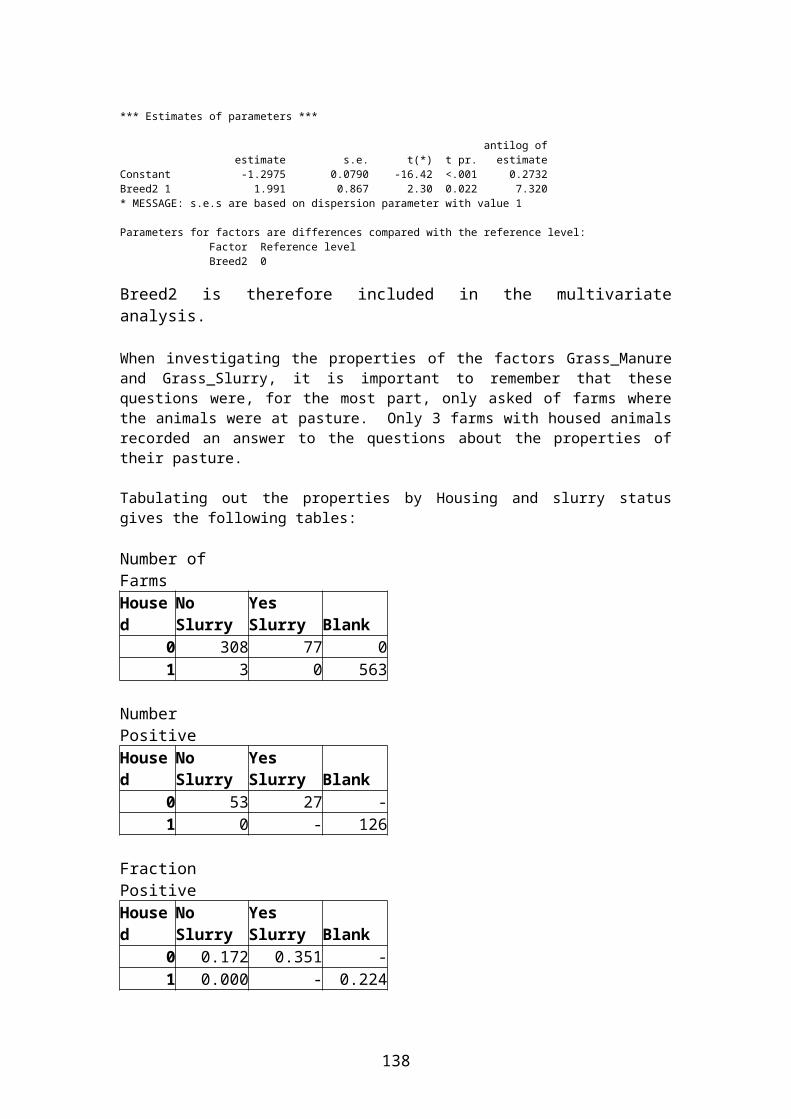
497 0.00 0.099 527 0.00 0.051 552 0.00 0.050 581 1.00 0.059 601 1.00 0.109 602 0.00 0.096 640 1.00 0.052 659 0.00 0.049 701 1.00 0.097 788 1.00 0.101 858 0.00 0.114 *** Estimates of parameters *** antilog of estimate s.e. t(*) t pr. estimateConstant -1.750 0.384 -4.55 <.001 0.1738FCattle 2 0.383 0.208 1.84 0.066 1.466FCattle 3 0.362 0.234 1.55 0.122 1.436FCattle 4 0.981 0.318 3.08 0.002 2.668SamGrF 2 0.746 0.266 2.81 0.005 2.109SamGrF 3 0.632 0.269 2.35 0.019 1.882SamGrF 4 1.097 0.268 4.09 <.001 2.995BeefonDairy 1 1.967 0.641 3.07 0.002 7.150Gra_Slur 1 1.201 0.319 3.76 <.001 3.324Gra_Slur 999 0.084 0.197 0.43 0.668 1.088Gra_Manu 1 -1.164 0.369 -3.15 0.002 0.3122Gra_Manu 999 0 * * * 1.000Pigs 2 0.891 0.347 2.57 0.010 2.438Max_Age -0.0309 0.0154 -2.01 0.044 0.9695* MESSAGE: s.e.s are based on dispersion parameter with value 1 Parameters for factors are differences compared with the reference level: Factor Reference level FCattle 1 SamGrF 1 BeefonDairy 0 Gra_Slur 0 Gra_Manu 0 Pigs 1
Hence, the factors FCattle, SamGrF, Beefin Dairy, Gra_Slurry, Gra_Manure, Pigs and the variate Max_Age are carried forward for detailed review in the Generalised Linear Mixed Model.
Fitting this model in the Generalised Linear Mixed Model context gives the following output. Initially, County and veterinary practice are fitted as possible random effects along with Farm.
5560 GLMM[PRINT=model,monitor,components,vcovariance,means,backmeans,effects;DISTRIBUTION=binomial;\5561 LINK=logit; DISPERSION=1; FIXED=SamGrF + Gra_Slur + Gra_Manu+BeefonDairy + Pigs + FCattle + Max_Age;\5562 RANDOM=County+Vet+Farm; CONSTANT=estimate; FACT=9; PSE=*;MAXCYCLE=20; FMETHOD=fixed;\5563 CADJUST=mean] VFarmPos; NBINOMIAL=N_Bin
**** G5W0001 **** Warning (Code VC 38). Statement 131 in Procedure GLMM
Command: REML [PRINT=*; RMETHOD=all] TRANSValue of deviance at final iteration larger than at previous iteration(s)
Minimum deviance = 2199.17: value at final iteration = 2215.26
**** G5W0002 **** Warning (Code VD 12). Statement 131 in Procedure GLMM
Command: REML [PRINT=*; RMETHOD=all] TRANSREML algorithm has diverged/parameters out of bounds - output not available
138

Results may be unreliable. Printed estimates of varianceparameters/monitoringinformation are available from REML or VDISPLAY and will indicate whichparameters are unstable. Redefine the model or use better initial values.
**** G5W0003 **** Warning (Code VD 12). Statement 135 in Procedure GLMM
Command: VKEEP #RAND; COMP=V[]REML algorithm has diverged/parameters out of bounds - output not available
Results may be unreliable. Printed estimates of varianceparameters/monitoringinformation are available from REML or VDISPLAY and will indicate whichparameters are unstable. Redefine the model or use better initial values.
* Message: Negative variance components present:
* Tables of effects/means will be produced for random model terms but shouldbeused with caution
***** Generalised Linear Mixed Model Analysis *****
Method: Marginal model, cf Breslow & Clayton (1993) JASA Response variate: VFarmPos Distribution: BINOMIAL Link function: LOGIT
Random model: (County + Vet) + Farm Fixed model: Constant + (((((SamGrF + Gra_Slur) + Gra_Manu) +BeefinDairy) + Pigs) + FCattle) + Max_Age
* Dispersion parameter fixed at value 1.000
******** Warning from GLMM: missing values generated in weights/working variate.
*** Monitoring information ***
Iteration Gammas Dispersion Max change 1 0.009026 0.0001000 0.2296 1.000 3.4670E+00
******** Warning from GLMM: missing values generated in weights/working variate.
2 0.005302 0.0001000 0.0001000 1.000 2.2952E-01
******** Warning from GLMM: missing values generated in weights/working variate.
3 0.005788 0.0001000 0.09561 1.000 9.5507E-02
******** Warning from GLMM: missing values generated in weights/working variate.
4 0.005703 0.0001000 0.2326 1.000 1.3699E-01
******** Warning from GLMM: missing values generated in weights/working variate.
5 0.005657 0.0001000 0.2370 1.000 4.3747E-03
******** Warning from GLMM: missing values generated in weights/working variate.
6 0.005638 0.0001000 0.2368 1.000 2.0973E-04
******** Warning from GLMM: missing values generated in weights/working variate.
139
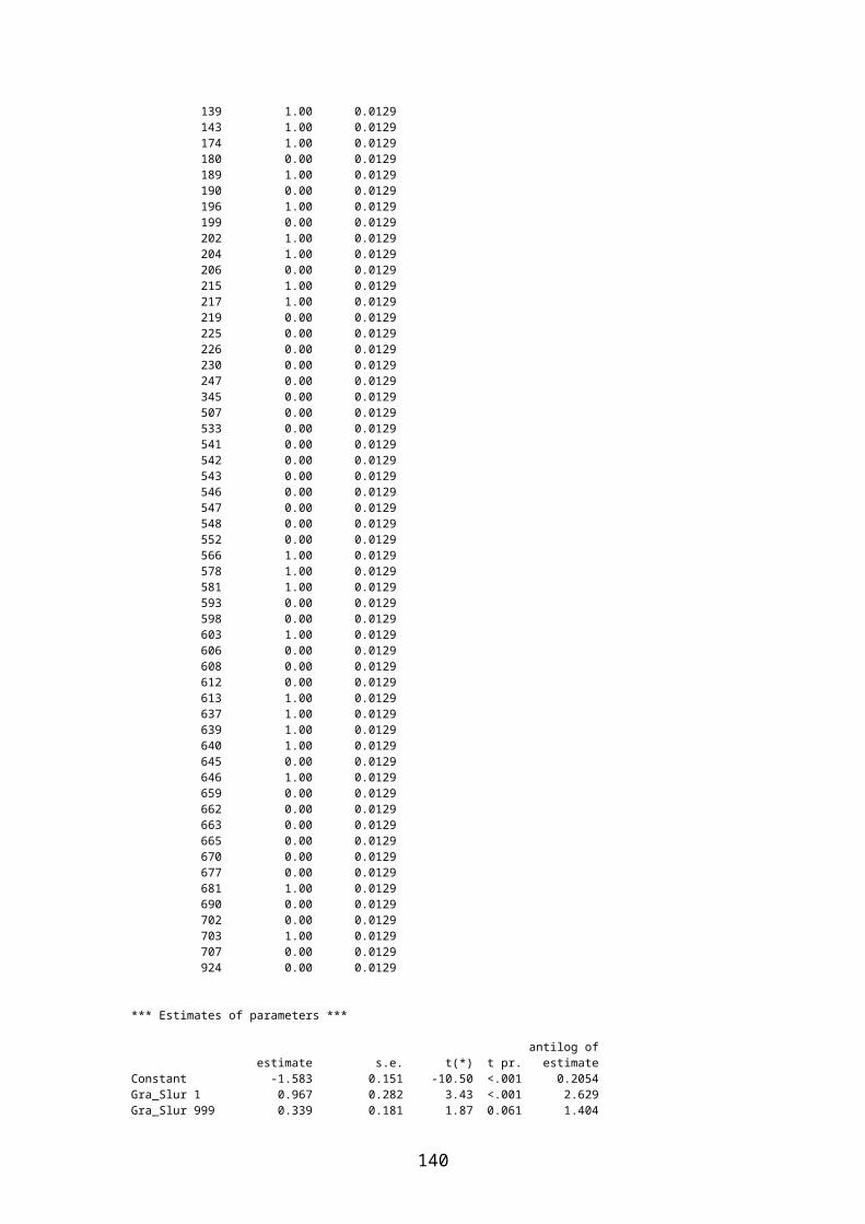
7 0.005635 0.0001000 0.2367 1.000 7.3462E-05
*** Estimated Variance Components ***
Random term Component S.e.
County 0.006 0.052Vet 0.000 0.093Farm 0.237 0.304
*** Residual variance model ***
Term Factor Model(order) Parameter EstimateS.e.
Dispersn Identity Sigma2 1.000FIXED
*** Estimated Variance matrix for Variance Components ***
County 1 0.00272 Vet 2 -0.00204 0.00858 Farm 3 -0.00034 -0.00654 0.09255 Dispersn 4 0.00000 0.00000 0.00000 0.00000
1 2 3 4
*** Table of effects for Constant ***
-2.349 Standard error: 0.2667
*** Table of effects for SamGrF ***
SamGrF 1 2 3 4 0.0000 0.7505 0.6321 1.0896
Standard error of differences: Average 0.2515 Maximum 0.2737 Minimum 0.2280
Average variance of differences: 0.06369
*** Table of effects for Gra_Slur ***
Gra_Slur 0.0 1.0 999.0 0.0000 1.2091 0.0885
Standard error of differences: Average 0.2846 Maximum 0.3277 Minimum 0.2011
Average variance of differences: 0.08451
*** Table of effects for Gra_Manu ***
Gra_Manu 0.0 1.0 999.0 0.0000 -1.1654 0.0000
Standard error of differences: 0.3776
*** Table of effects for BeefonDairy ***
BeefonDairy 0.0000 1.0000 0.0000 1.9659
140

Standard error of differences: 0.6598
*** Table of effects for Pigs ***
Pigs 1 2 0.0000 0.8876
Standard error of differences: 0.3565
*** Table of effects for FCattle ***
FCattle 1 2 3 4 0.0000 0.3834 0.3564 0.9813
Standard error of differences: Average 0.2796 Maximum 0.3352 Minimum 0.2130
Average variance of differences: 0.08062
*** Table of effects for Max_Age ***
-0.03106 Standard error: 0.015738
**** G5W0004 **** Warning (Code VC 19). Statement 268 in Procedure GLMM
Command: VKEEP #PFORM; MEANS=MEANS[]; VARMEANS=VARMEANS[]Table/sed matrix not available for mean effects of covariates
Table of mean effects cannot be saved for term Max_Ageas it is a variate/covariate
*** Tables of means ***
* Using covariate mean values
*** Table of predicted means for SamGrF ***
SamGrF 1 2 3 4 -0.4479 0.3025 0.1842 0.6417
*** Table of predicted means for Gra_Slur ***
Gra_Slur 0.0 1.0 999.0 -0.2624 0.9467 -0.1740
*** Table of predicted means for Gra_Manu ***
Gra_Manu 0.0 1.0 999.0 0.5586 -0.6068 0.5586
*** Table of predicted means for BeefonDairy ***
BeefonDairy 0.0000 1.0000 -0.8129 1.1531
*** Table of predicted means for Pigs ***
141

Pigs 1 2 -0.2737 0.6139
*** Table of predicted means for FCattle ***
FCattle 1 2 3 4 -0.2602 0.1233 0.0962 0.7212
*** Back-transformed Means (on the original scale) ***
* Using covariate mean values
SamGrF 1 0.3899 2 0.5751 3 0.5459 4 0.6551
Gra_Slur 0.0 0.4348 1.0 0.7204 999.0 0.4566
Gra_Manu 0.0 0.6361 1.0 0.3528 999.0 0.6361
BeefonDairy 0.0000 0.3073 1.0000 0.7601
Pigs 1 0.4320 2 0.6488
FCattle 1 0.4353 2 0.5308 3 0.5240 4 0.6729
Note: means are probabilities not expected values.
Veterinary practice is clearly the least significant (in fact, virtually non-existent) variance component. The model is refitted without this random factor.5564 GLMM[PRINT=model,monitor,components,vcovariance,means,backmeans,effects;DISTRIBUTION=binomial;\5565 LINK=logit; DISPERSION=1; FIXED=SamGrF + Gra_Slur + Gra_Manu+BeefonDairy + Pigs + FCattle + Max_Age;\5566 RANDOM=County+Farm; CONSTANT=estimate; FACT=9; PSE=*; MAXCYCLE=20;FMETHOD=fixed;\5567 CADJUST=mean] VFarmPos; NBINOMIAL=N_Bin
* Message: Negative variance components present:
* Tables of effects/means will be produced for random model terms but shouldbeused with caution
***** Generalised Linear Mixed Model Analysis *****
142

Method: Marginal model, cf Breslow & Clayton (1993) JASA Response variate: VFarmPos Distribution: BINOMIAL Link function: LOGIT
Random model: County + Farm Fixed model: Constant + (((((SamGrF + Gra_Slur) + Gra_Manu) +BeefinDairy) + Pigs) + FCattle) + Max_Age
* Dispersion parameter fixed at value 1.000
******** Warning from GLMM: missing values generated in weights/working variate.
*** Monitoring information ***
Iteration Gammas Dispersion Max change 1 0.0001000 0.1210 1.000 3.5292E+00
******** Warning from GLMM: missing values generated in weights/working variate.
2 0.0001000 0.0001000 1.000 1.2092E-01
******** Warning from GLMM: missing values generated in weights/working variate.
3 0.0001000 0.0001000 1.000 0.0000E+00
*** Estimated Variance Components ***
Random term Component S.e.
County 0.000 0.042Farm 0.000 0.278
*** Residual variance model ***
Term Factor Model(order) Parameter EstimateS.e.
Dispersn Identity Sigma2 1.000FIXED
*** Estimated Variance matrix for Variance Components ***
County 1 0.00173 Farm 2 -0.00160 0.07753 Dispersn 3 0.00000 0.00000 0.00000
1 2 3
*** Table of effects for Constant ***
-2.345 Standard error: 0.2540
*** Table of effects for SamGrF ***
SamGrF 1 2 3 4 0.0000 0.7439 0.6306 1.0895
Standard error of differences: Average 0.2424 Maximum 0.2623 Minimum 0.2212
Average variance of differences: 0.05914
143

*** Table of effects for Gra_Slur ***
Gra_Slur 0.0 1.0 999.0 0.0000 1.2053 0.0917
Standard error of differences: Average 0.2747 Maximum 0.3156 Minimum 0.1946
Average variance of differences: 0.07864
*** Table of effects for Gra_Manu ***
Gra_Manu 0.0 1.0 999.0 0.0000 -1.1552 0.0000
Standard error of differences: 0.3589
*** Table of effects for BeefonDairy ***
BeefonDairy 0.0000 1.0000 0.0000 1.9648
Standard error of differences: 0.6380
*** Table of effects for Pigs ***
Pigs 1 2 0.0000 0.8917
Standard error of differences: 0.3454
*** Table of effects for FCattle ***
FCattle 1 2 3 4 0.0000 0.3818 0.3515 0.9802
Standard error of differences: Average 0.2710 Maximum 0.3254 Minimum 0.2062
Average variance of differences: 0.07578
*** Table of effects for Max_Age ***
-0.03085 Standard error: 0.015202
**** G5W0005 **** Warning (Code VC 19). Statement 268 in Procedure GLMM
Command: VKEEP #PFORM; MEANS=MEANS[]; VARMEANS=VARMEANS[]Table/sed matrix not available for mean effects of covariates
Table of mean effects cannot be saved for term Max_Ageas it is a variate/covariate
*** Tables of means ***
* Using covariate mean values
144

*** Table of predicted means for SamGrF ***
SamGrF 1 2 3 4 -0.4409 0.3030 0.1897 0.6486
*** Table of predicted means for Gra_Slur ***
Gra_Slur 0.0 1.0 999.0 -0.2572 0.9481 -0.1655
*** Table of predicted means for Gra_Manu ***
Gra_Manu 0.0 1.0 999.0 0.5602 -0.5950 0.5602
*** Table of predicted means for BeefonDairy ***
BeefonDairy 0.0000 1.0000 -0.8073 1.1575
*** Table of predicted means for Pigs ***
Pigs 1 2 -0.2707 0.6210
*** Table of predicted means for FCattle ***
FCattle 1 2 3 4 -0.2533 0.1286 0.0982 0.7270
*** Back-transformed Means (on the original scale) ***
* Using covariate mean values
SamGrF 1 0.3915 2 0.5752 3 0.5473 4 0.6567
Gra_Slur 0.0 0.4360 1.0 0.7207 999.0 0.4587
Gra_Manu 0.0 0.6365 1.0 0.3555 999.0 0.6365
BeefonDairy 0.0000 0.3085 1.0000 0.7609
Pigs 1 0.4327 2 0.6504
FCattle 1 0.4370 2 0.5321
145

3 0.5245 4 0.6741
Note: means are probabilities not expected values.
Neither variance component is significantly affecting the model. It would seem sensible, however, to attempt to fit the model with only the lowest stratum of variability.5568 GLMM[PRINT=model,monitor,components,vcovariance,means,backmeans,effects;DISTRIBUTION=binomial;\5569 LINK=logit; DISPERSION=1; FIXED=SamGrF + Gra_Slur + Gra_Manu+BeefonDairy + Pigs + FCattle + Max_Age;\5570 RANDOM=Farm; CONSTANT=estimate; FACT=9; PSE=*; MAXCYCLE=20;FMETHOD=fixed;\5571 CADJUST=mean] VFarmPos; NBINOMIAL=N_Bin
***** Generalised Linear Mixed Model Analysis *****
Method: Marginal model, cf Breslow & Clayton (1993) JASA Response variate: VFarmPos Distribution: BINOMIAL Link function: LOGIT
Random model: Farm Fixed model: Constant + (((((SamGrF + Gra_Slur) + Gra_Manu) +BeefinDairy) + Pigs) + FCattle) + Max_Age
* Dispersion parameter fixed at value 1.000
******** Warning from GLMM: missing values generated in weights/working variate.
*** Monitoring information ***
Iteration Gammas Dispersion Max change 1 0.09728 1.000 3.5426E+00
******** Warning from GLMM: missing values generated in weights/working variate.
2 0.0001000 1.000 9.7176E-02
******** Warning from GLMM: missing values generated in weights/working variate.
3 0.0001000 1.000 0.0000E+00
*** Estimated Variance Components ***
Random term Component S.e.
Farm 0.000 0.276
*** Residual variance model ***
Term Factor Model(order) Parameter EstimateS.e.
Dispersn Identity Sigma2 1.000FIXED
*** Estimated Variance matrix for Variance Components ***
Farm 1 0.07605 Dispersn 2 0.00000 0.00000
146

1 2
*** Table of effects for Constant ***
-2.345 Standard error: 0.2540
*** Table of effects for SamGrF ***
SamGrF 1 2 3 4 0.0000 0.7439 0.6307 1.0896
Standard error of differences: Average 0.2424 Maximum 0.2623 Minimum 0.2212
Average variance of differences: 0.05914
*** Table of effects for Gra_Slur ***
Gra_Slur 0.0 1.0 999.0 0.0000 1.2053 0.0917
Standard error of differences: Average 0.2746 Maximum 0.3156 Minimum 0.1946
Average variance of differences: 0.07863
*** Table of effects for Gra_Manu ***
Gra_Manu 0.0 1.0 999.0 0.0000 -1.1552 0.0000
Standard error of differences: 0.3589
*** Table of effects for BeefonDairy ***
BeefonDairy 0.0000 1.0000 0.0000 1.9648
Standard error of differences: 0.6380
*** Table of effects for Pigs ***
Pigs 1 2 0.0000 0.8918
Standard error of differences: 0.3454
*** Table of effects for FCattle ***
FCattle 1 2 3 4 0.0000 0.3818 0.3515 0.9802
Standard error of differences: Average 0.2710 Maximum 0.3254 Minimum 0.2062
Average variance of differences: 0.07578
*** Table of effects for Max_Age ***
-0.03085 Standard error: 0.015201
147

**** G5W0006 **** Warning (Code VC 19). Statement 268 in Procedure GLMM
Command: VKEEP #PFORM; MEANS=MEANS[]; VARMEANS=VARMEANS[]Table/sed matrix not available for mean effects of covariates
Table of mean effects cannot be saved for term Max_Ageas it is a variate/covariate
*** Tables of means ***
* Using covariate mean values
*** Table of predicted means for SamGrF ***
SamGrF 1 2 3 4 -0.4408 0.3031 0.1898 0.6487
*** Table of predicted means for Gra_Slur ***
Gra_Slur 0.0 1.0 999.0 -0.2571 0.9481 -0.1654
*** Table of predicted means for Gra_Manu ***
Gra_Manu 0.0 1.0 999.0 0.5603 -0.5949 0.5603
*** Table of predicted means for BeefonDairy ***
BeefonDairy 0.0000 1.0000 -0.8072 1.1576
*** Table of predicted means for Pigs ***
Pigs 1 2 -0.2707 0.6211
*** Table of predicted means for FCattle ***
FCattle 1 2 3 4 -0.2532 0.1287 0.0983 0.7270
*** Back-transformed Means (on the original scale) ***
* Using covariate mean values
SamGrF 1 0.3915 2 0.5752 3 0.5473 4 0.6567
Gra_Slur 0.0 0.4361 1.0 0.7207 999.0 0.4587
148
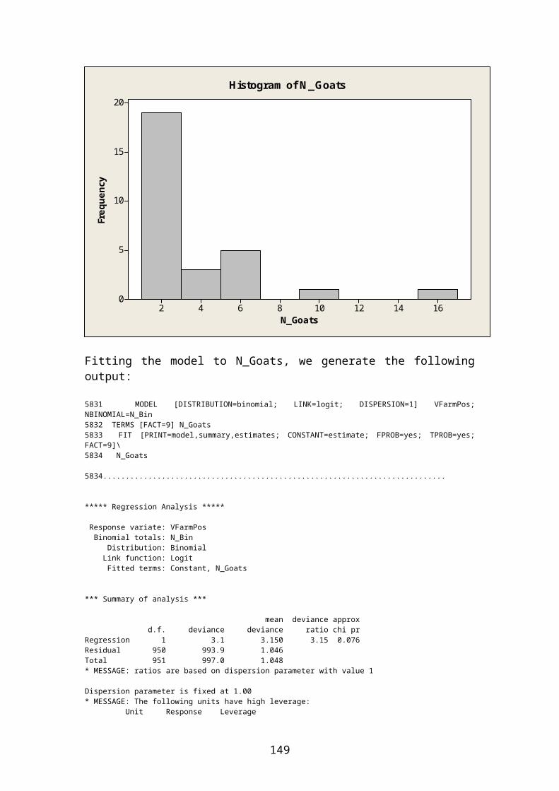
Gra_Manu 0.0 0.6365 1.0 0.3555 999.0 0.6365
BeefonDairy 0.0000 0.3085 1.0000 0.7609
Pigs 1 0.4327 2 0.6505
FCattle 1 0.4370 2 0.5321 3 0.5246 4 0.6742
Note: means are probabilities not expected values.
Given the complete lack of significance of the Farm effect, it was thought worthwhile to investigate the equivalent model incorporating County as the sole random effect. 5576 GLMM[PRINT=model,monitor,components,vcovariance,means,backmeans,effects;DISTRIBUTION=binomial;\5577 LINK=logit; DISPERSION=1; FIXED=SamGrF + Gra_Slur + Gra_Manu+BeefonDairy + Pigs + FCattle + Max_Age;\5578 RANDOM=County; CONSTANT=estimate; FACT=9; PSE=*; MAXCYCLE=20;FMETHOD=fixed;\5579 CADJUST=mean] VFarmPos; NBINOMIAL=N_Bin
* Message: Negative variance components present:
* Tables of effects/means will be produced for random model terms but shouldbeused with caution
***** Generalised Linear Mixed Model Analysis *****
Method: Marginal model, cf Breslow & Clayton (1993) JASA Response variate: VFarmPos Distribution: BINOMIAL Link function: LOGIT
Random model: County Fixed model: Constant + (((((SamGrF + Gra_Slur) + Gra_Manu) +BeefinDairy) + Pigs) + FCattle) + Max_Age
* Dispersion parameter fixed at value 1.000
******** Warning from GLMM: missing values generated in weights/working variate.
*** Monitoring information ***
Iteration Gammas Dispersion Max change 1 0.0001000 1.000 1.1357E-02
******** Warning from GLMM: missing values generated in weights/working variate.
2 0.0001000 1.000 0.0000E+00
*** Estimated Variance Components ***
149

Random term Component S.e.
County 0.000 0.036
*** Residual variance model ***
Term Factor Model(order) Parameter EstimateS.e.
Dispersn Identity Sigma2 1.000FIXED
*** Estimated Variance matrix for Variance Components ***
County 1 0.0012650 Dispersn 2 0.0000000 0.0000000
1 2
*** Table of effects for Constant ***
-2.235 Standard error: 0.2221
*** Table of effects for SamGrF ***
SamGrF 1 2 3 4 0.0000 0.6742 0.5690 1.0116
Standard error of differences: Average 0.2221 Maximum 0.2363 Minimum 0.2097
Average variance of differences: 0.04944
*** Table of effects for Gra_Slur ***
Gra_Slur 0.0 1.0 999.0 0.0000 1.1463 0.0813
Standard error of differences: Average 0.2590 Maximum 0.2994 Minimum 0.1803
Average variance of differences: 0.07020
*** Table of effects for Gra_Manu ***
Gra_Manu 0.0 1.0 999.0 0.0000 -1.0643 0.0000
Standard error of differences: 0.3138
*** Table of effects for BeefonDairy ***
BeefonDairy 0.0000 1.0000 0.0000 1.9072
Standard error of differences: 0.6258
*** Table of effects for Pigs ***
Pigs 1 2 0.0000 0.8653
150

Standard error of differences: 0.3371
*** Table of effects for FCattle ***
FCattle 1 2 3 4 0.0000 0.3586 0.3300 0.9417
Standard error of differences: Average 0.2587 Maximum 0.3151 Minimum 0.1918
Average variance of differences: 0.06943
*** Table of effects for Max_Age ***
-0.02929 Standard error: 0.014025
******** Warning (Code VC 19). Statement 268 in Procedure GLMM
Command: VKEEP #PFORM; MEANS=MEANS[]; VARMEANS=VARMEANS[]Table/sed matrix not available for mean effects of covariates
Table of mean effects cannot be saved for term Max_Ageas it is a variate/covariate
*** Tables of means ***
* Using covariate mean values
*** Table of predicted means for SamGrF ***
SamGrF 1 2 3 4 -0.3868 0.2874 0.1822 0.6248
*** Table of predicted means for Gra_Slur ***
Gra_Slur 0.0 1.0 999.0 -0.2322 0.9140 -0.1510
*** Table of predicted means for Gra_Manu ***
Gra_Manu 0.0 1.0 999.0 0.5317 -0.5326 0.5317
*** Table of predicted means for BeefonDairy ***
BeefonDairy 0.0000 1.0000 -0.7767 1.1305
*** Table of predicted means for Pigs ***
Pigs 1 2 -0.2557 0.6096
*** Table of predicted means for FCattle ***
FCattle 1 2 3 4 -0.2307 0.1280 0.0993 0.7111
151
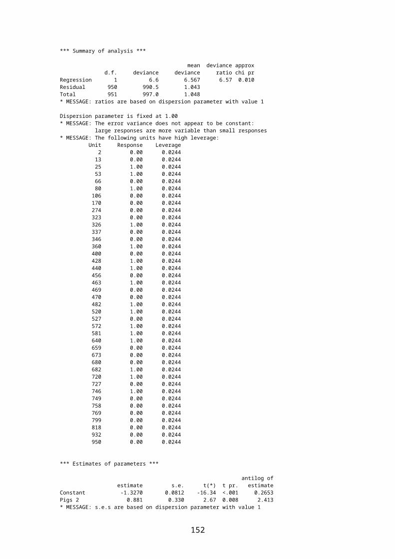
*** Back-transformed Means (on the original scale) ***
* Using covariate mean values
SamGrF 1 0.4045 2 0.5714 3 0.5454 4 0.6513
Gra_Slur 0.0 0.4422 1.0 0.7138 999.0 0.4623
Gra_Manu 0.0 0.6299 1.0 0.3699 999.0 0.6299
BeefonDairy 0.0000 0.3150 1.0000 0.7559
Pigs 1 0.4364 2 0.6478
FCattle 1 0.4426 2 0.5320 3 0.5248 4 0.6706
Note: means are probabilities not expected values.
Hence there is no evidence of any of the random effects being particularly important. However, it would seem sensible to use a REML-type algorithm to fit the data, given the strongly unbalanced nature of the dataset. Hence, we will fit the model with Farm as the sole random effect. Refitting the model (output not listed) and calculating Wald statistics for the fixed effects gives the following results:
5582 VDISPLAY [PRINT=Wald] 5582............................................................................ *** Wald tests for fixed effects *** Fixed term Wald statistic d.f. Wald/d.f. Chi-sq prob * Sequentially adding terms to fixed model SamGrF 26.59 3 8.86 <0.001 Gra_Slur 9.38 2 4.69 0.009 Gra_Manu 9.17 1 9.17 0.002 BeefonDairy 8.10 1 8.10 0.004 Pigs 5.21 1 5.21 0.022 FCattle 7.79 3 2.60 0.051 Max_Age 4.12 1 4.12 0.042 * Dropping individual terms from full fixed model
152

SamGrF 17.56 3 5.85 <0.001 Gra_Slur 15.20 2 7.60 <0.001 Gra_Manu 10.36 1 10.36 0.001 BeefonDairy 9.48 1 9.48 0.002 Pigs 6.67 1 6.67 0.010 FCattle 10.36 3 3.45 0.016 Max_Age 4.12 1 4.12 0.042 * Message: chi-square distribution for Wald tests is an asymptotic approximation (i.e. for large samples) and underestimates the probabilities in other cases.
Even allowing for the liberal nature of the Wald tests, it is clear that there is strong statistical evidence for the inclusion of each of the factors in the final multi-factor model.
Each factor will be reviewed in turn, plotting the mean estimated farm prevalence for different levels of each factor, along with the associated 95% confidence intervals.
Considering SamGrF, there is clear evidence that farms with fewer than 12 animals in the sampling group have a lower probability of exhibiting shedding.
Category Mean Farm Prevalence<12 0.39
12-17 0.5818-28 0.55>28 0.66
Any trend in the data would be assumed to be monotonic, and hence it seems likely that the (statistically insignificant) difference between categories 2 and 3 is simply due to stochastic noise. It is not immediately clear how the prevalence in the highest category relates to those in the intermediate categories.
0
0.2
0.4
0.6
0.8
1
<12 12-17 18-28 >28
Categories
Mea
n Fa
rm P
reva
lenc
e
153

Contrasting the mean in the first category with the means in the 2 intermediate categories, we find that the mean difference (on the logit scale) equals 0.69, the standard error is 0.23 and hence the t-statistic equals 2.93, with an associated p-value of 0.003. Hence, the probability of detecting shedding is lower in groups containing fewer than 12 animals than in groups containing 12-28 animals. Contrasting the mean in the final category with the means in the 2 intermediate categories, we find that the mean difference on the logit scale equals 0.40, the standard error is 0.19 and hence the t-statistic equals 2.12, with an associated p-value of 0.03. Hence, the probability of detecting shedding is lower in groups containing 12-28 animals than in groups containing more animals.
It might be thought that this is a truism: that if on all farms, each animal has an independent chance of shedding, and hence the larger the number of samples tested, the more likely it is that a positive sample will be detected. In practice, we might suspect that the independence assumption is extremely unlikely to be true, but we need to assess the results under such a hypothesis. The first requirement is to estimate the independent probability of animal infection. For each category, we tabulate the median number of samples collected, and hence, based on the estimated farm prevalences for these categories, an estimate of the individual probabilities.
CategoryMean
PrevalenceMedian Samples
Individual Probability
<12 0.39 8 0.06012-17 0.58 14 0.05918-28 0.55 18 0.043
>28 0.66 22 0.047
The higher the number of samples in the sample, the weaker the effect of variability in the sampling distribution on the individual probabilities. However, the Highest category is unbounded, which will increase the variability again. On this basis, a value of 0.043, derived from the 18-28 category, is used as the estimate of the individual probability.
Category
Estimated Prevalence from Data
Modelled Prevalence
<12 0.39 0.3012-17 0.58 0.4618-28 0.55 0.55
>28 0.66 0.62
Given the sizeable numbers of farms in the study, the differences between the estimated and modelled prevalences in the lowest two categories are appreciable. Similar results were generated by calculating the individual probability of detection for each farm, and then averaging these by category. On this basis, it seems unlikely that the pattern of prevalences associated with SamGrF are purely explicable as being a mechanical association with the highly correlated term, number of samples collected. Besides which, the within-herd prevalence estimated here is very much less than that calculated from the within-herd prevalence data. This must cast
154

considerable doubt on the argument that this observed effect is an artefact of the sampling scheme. However, this possibility should be taken into account when discussing this variable. However, the inclusion of FCattle in the model, even in the presence of SamGrF, indicates that there are genuine ‘size of operation’ effects present in the epidemiology of infection.
In view of this, we will next consider the factor FCattle. The pattern of prevalence can be seen in the following diagram:
0
0.2
0.4
0.6
0.8
1
1-49 50-99 100-199 200+
Categories
Mea
n Fa
rm P
reva
lenc
e
The mean farm prevalences for each category of FCattle are as follows:
Category Mean Farm Prevalence1-49 0.4450-99 0.53
100-199 0.52200+ 0.67
There is some indication of an upwards trend in the data with respect to higher numbers of finishing cattle, especially when comparing the lowest category, the middle two categories and the highest category.
Comparing the lowest category (<50 animals) with the two intermediate categories (50-99 and 100-199), the mean difference in prevalences (on the logit scale) is 0.37, with a standard error of 0.19, giving rise to a t-statistic of 1.98 and an associated p-value of 0.048. Comparing the intermediate categories with the highest category (200+ animals), the mean difference in prevalences (on the logit scale) is 0.61, with a standard error of 0.30, giving rise to a t-statistic of 2.07 and an associated p-value of 0.039. Hence, there is evidence of a trend of increased risk of shedding being identified, associated with higher numbers of finishing cattle on the farm. In the context of SamGrF also being fitted to the model, this result is almost certainly a genuine effect of enterprise size. It might be associated with some threshold results
155

from epidemic modelling theory, or from some aspects of animal management on larger enterprises.
Next, considering the effect of spreading slurry on pasture. It will be remembered that this question was in the main asked only to farms with animals at pasture. Hence, the inclusion in this analysis of a ‘Housed’ category, to reflect the prevalences seen, on average, on farms on which the question was not asked. The mean prevalences for the different categories are as follows:
CategoryMean Farm Prevalence
Unhoused: No Slurry 0.44Unhoused: Slurry Spread 0.72
Housed 0.46
It is apparent that the mean prevalences seen in Housed animals and in Pastured animals from farms which do not spread slurry are virtually identical. However, the mean prevalence on farms which do spread slurry is appreciably higher. Comparing the mean prevelences on farms with animals at pasture, comparing those which spread slurry and those which do not, we find that the mean difference (on the logit scale) equals 1.21, the standard error equals 0.32, giving rise to a t-statistic of 3.82 and an associated p-value less than 0.001. The spreading of slurry on pasture is a significant risk factor on farms with animals at pasture.
0
0.2
0.4
0.6
0.8
1
Unhoused: No Slurry Unhoused: SlurrySpread
Housed
Categories
Mea
n Fa
rm P
reva
lenc
e
Next, we consider the effect of spreading manure on pasture. Again, this question was in the main asked only to farms with animals at pasture. Hence, the repeated inclusion in this analysis of a ‘Housed’ category, to reflect the prevalences seen, on average, on farms on which the question was not asked.
156

0
0.2
0.4
0.6
0.8
1
Unhoused: No Manure Unhoused: ManureSpread
Housed
Categories
Mea
n Fa
rm P
reva
lenc
e
The mean farm prevalences for the different categories of farm are as follows:
CategoryMean Farm Prevalence
Unhoused: No Manure 0.64Unhoused: Manure Spread 0.36
Housed 0.64
It is apparent that the mean prevalences seen in Housed animals and in Pastured animals from farms which do not spread manure are virtually identical. However, the mean prevalence on farms which do spread manure is appreciably lower. Comparing the mean prevelences on farms with animals at pasture, comparing those which spread manure and those which do not, we find that the mean difference (on the logit scale) equals 1.16, the standard error equals 0.36, giving rise to a t-statistic of 3.22 and an associated p-value of 0.001. The spreading of manure on pasture is a significant protective factor on farms with animals at pasture. This result may appear somewhat counterintuitive: however, it may be related to the manure management regime in place on a farm which wishes to spread this material on pasture. If the regimen which is put in place to achieve this reduces contact of animals with faeces in the short term during time periods when the animals are housed, this may have a negative effect on the ability of the infection to maintain itself on the farm, and hence it gives rise to a reduction in farm prevalence even later, when the animals (ironically) are at pasture, and hence in contact with the manure. The results seen earlier in the within-herd prevalence analysis would suggest that the contact of animals with infection while housed is more important in maintaining high prevalence levels than any contact while at pasture. It is unfortunate that the design of the study does not allow any investigation of whether similar manure on pasture effects are present on farms with (currently) housed animals.
157

Farms with beef animals in a dairy herd were identified as high risk in the earlier analyses. Considering the BeefonDairy factor, it is immediately clear that the prevalence is much higher on this class of farm.
CategoryMean Farm Prevalence
Not a Dairy Farm with Beef Cattle 0.31Dairy Farm with Beef Cattle 0.76
The means and 95% confidence intervals are given in the following plot:
0
0.2
0.4
0.6
0.8
1
Not a Dairy Farm with Beef Cattle Dairy Farm with Beef Cattle
Categories
Mea
n Fa
rm P
reva
lenc
e
Carrying out a t-test, the mean difference (on the logit scale) is found to be 1.96, the standard error is 0.64, the t-statistic equals 3.08, and the associated p-value 0.002. Hence, the prevalence is highly statistically significantly higher in this class of farm. It is of some concern that this particular group was only identified through a detailed examination of the data, but the high prevalence seen in this group is extremely striking.
The final factor which has been examined is Pigs. The mean farm prevalence for each category is as follows:
CategoryMean Farm Prevalence
Pigs not present 0.43Pigs present 0.65
The picture becomes more clear if the means are plotted with the associated 95% confidence intervals:
158

0
0.2
0.4
0.6
0.8
1
Pigs not present Pigs present
Categories
Mea
n Fa
rm P
reva
lenc
e
The data would suggest that farms with pigs present exhibit a higher prevalence than those which do not. Carrying out a t-test, the mean difference (on the logit scale) is found to be 0.89, the standard error is 0.35, the t-statistic equals 2.58, and the associated p-value 0.01. Hence, the prevalence is statistically significantly higher in this class of farm.
The only variate which has been included in the model is Max_Age. The effect of this variate on the linear predictor is summarised by the associated coefficient, which takes the estimated value of –0.03, with a standard error of 0.015. The associated p-value equals 0.04. Hence, this result suggests that the higher the maximum age of animal present in the sampling group, the less likely is the group to present a positive sample. The nature of the effect is similar to that seen in the univariate analysis, where the associated p-value was 0.30. However, the removal of noise through the fitting of other explanatory factors has clearly allowed the multi-factor model to identify the utility of this variate in explaining aspects of the data. A review of the histogram of the variate would suggest that it is unlikely to be subject to issues of leverage.
Having fitted all the likely explanatory variables in the multifactor model, we now return to explore the effect that the inclusion of these factors may have on the fit of the structural factors.
Fitting Division in addition to the above explanatory variables gives the following output:
5567 GLMM [PRINT=model,monitor,components,vcovariance,means,backmeans,effects; DISTRIBUTION=binomial;\5568 LINK=logit; DISPERSION=1; FIXED=SamGrF + Gra_Slur + Gra_Manu+BeefonDairy + Pigs + FCattle + Max_Age+Division;\5569 RANDOM=Farm; CONSTANT=estimate; FACT=9; PSE=*; MAXCYCLE=20; FMETHOD=fixed; CADJUST=mean] VFarmPos; NBINOMIAL=N_Bin ***** Generalised Linear Mixed Model Analysis *****
159

Method: Marginal model, cf Breslow & Clayton (1993) JASA Response variate: VFarmPos Distribution: BINOMIAL Link function: LOGIT Random model: Farm Fixed model: Constant + ((((((SamGrF + Gra_Slur) + Gra_Manu) + BeefinDairy) + Pigs) + FCattle) + Max_Age) + Division * Dispersion parameter fixed at value 1.000 ******** Warning from GLMM: missing values generated in weights/working variate. *** Monitoring information *** Iteration Gammas Dispersion Max change 1 0.1286 1.000 3.5100E+00 ******** Warning from GLMM: missing values generated in weights/working variate. 2 0.000001000 1.000 1.2864E-01 ******** Warning from GLMM: missing values generated in weights/working variate. 3 0.000001000 1.000 0.0000E+00 *** Estimated Variance Components *** Random term Component S.e. Farm 0.000 0.277 *** Residual variance model *** Term Factor Model(order) Parameter Estimate S.e. Dispersn Identity Sigma2 1.000 FIXED *** Estimated Variance matrix for Variance Components *** Farm 1 0.07674 Dispersn 2 0.00000 0.00000 1 2 *** Table of effects for Constant *** -2.144 Standard error: 0.3003 *** Table of effects for SamGrF *** SamGrF 1 2 3 4 0.0000 0.7174 0.5415 1.0466 Standard error of differences: Average 0.2447 Maximum 0.2661 Minimum 0.2227 Average variance of differences: 0.06023 *** Table of effects for Gra_Slur *** Gra_Slur 0.0 1.0 999.0
160

0.0000 1.2801 0.0802 Standard error of differences: Average 0.2790 Maximum 0.3217 Minimum 0.1955 Average variance of differences: 0.08130 *** Table of effects for Gra_Manu *** Gra_Manu 0.0 1.0 999.0 0.0000 -1.1381 0.0000 Standard error of differences: 0.3610 *** Table of effects for BeefonDairy *** BeefonDairy 0.0000 1.0000 0.000 2.015 Standard error of differences: 0.6400 *** Table of effects for Pigs *** Pigs 1 2 0.0000 0.8741 Standard error of differences: 0.3480 *** Table of effects for FCattle *** FCattle 1 2 3 4 0.0000 0.3680 0.3494 0.9796 Standard error of differences: Average 0.2747 Maximum 0.3277 Minimum 0.2076 Average variance of differences: 0.07788 *** Table of effects for Max_Age *** -0.03181 Standard error: 0.015407 *** Table of effects for Division *** Division Central Highland Islands North East South East 0.0000 -0.4960 -0.2883 0.0093 0.0066 Division South West -0.3872 Standard error of differences: Average 0.3212 Maximum 0.4244 Minimum 0.2437 Average variance of differences: 0.1062 **** G5W0003 **** Warning (Code VC 19). Statement 268 in Procedure GLMM Command: VKEEP #PFORM; MEANS=MEANS[]; VARMEANS=VARMEANS[]Table/sed matrix not available for mean effects of covariates
161
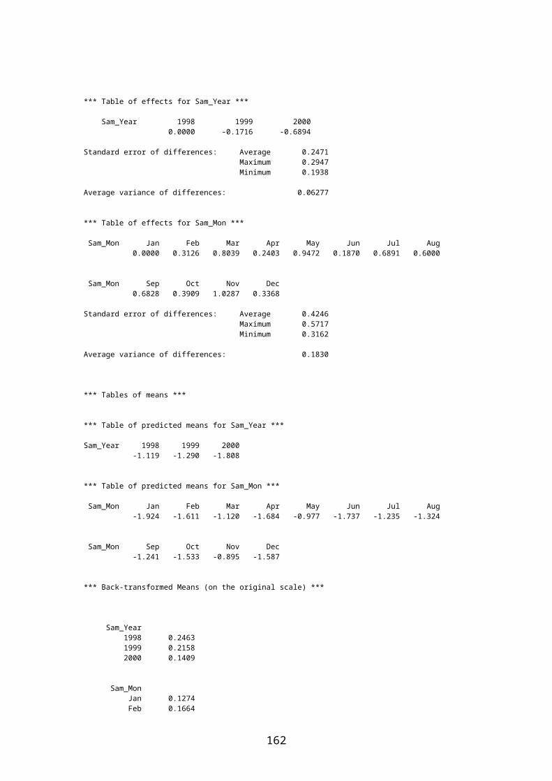
Table of mean effects cannot be saved for term Max_Ageas it is a variate/covariate *** Tables of means *** * Using covariate mean values *** Table of predicted means for SamGrF *** SamGrF 1 2 3 4 -0.3942 0.3232 0.1473 0.6524 *** Table of predicted means for Gra_Slur *** Gra_Slur 0.0 1.0 999.0 -0.2713 1.0088 -0.1911 *** Table of predicted means for Gra_Manu *** Gra_Manu 0.0 1.0 999.0 0.5615 -0.5766 0.5615 *** Table of predicted means for BeefonDairy *** BeefonDairy 0.0000 1.0000 -0.825 1.189 *** Table of predicted means for Pigs *** Pigs 1 2 -0.2549 0.6192 *** Table of predicted means for FCattle *** FCattle 1 2 3 4 -0.2421 0.1259 0.1073 0.7375 *** Table of predicted means for Division *** Division Central Highland Islands North East South East 0.3748 -0.1213 0.0864 0.3841 0.3814 Division South West -0.0124 *** Back-transformed Means (on the original scale) *** * Using covariate mean values SamGrF 1 0.4027 2 0.5801 3 0.5367 4 0.6575 Gra_Slur 0.0 0.4326 1.0 0.7328 999.0 0.4524
162

Gra_Manu 0.0 0.6368 1.0 0.3597 999.0 0.6368 BeefonDairy 0.0000 0.3047 1.0000 0.7666 Pigs 1 0.4366 2 0.6500 FCattle 1 0.4398 2 0.5314 3 0.5268 4 0.6764 Division Central 0.5926 Highland 0.4697 Islands 0.5216 North East 0.5949 South East 0.5942 South West 0.4969 Note: means are probabilities not expected values. 5570 VDISPLAY [PRINT=Wald] 5570............................................................................ *** Wald tests for fixed effects *** Fixed term Wald statistic d.f. Wald/d.f. Chi-sq prob * Sequentially adding terms to fixed model SamGrF 26.27 3 8.76 <0.001 Gra_Slur 9.23 2 4.61 0.010 Gra_Manu 9.05 1 9.05 0.003 BeefonDairy 8.03 1 8.03 0.005 Pigs 5.15 1 5.15 0.023 FCattle 7.56 3 2.52 0.056 Max_Age 4.05 1 4.05 0.044 Division 5.56 5 1.11 0.352 * Dropping individual terms from full fixed model SamGrF 16.43 3 5.48 <0.001 Gra_Slur 16.61 2 8.31 <0.001 Gra_Manu 9.94 1 9.94 0.002 BeefonDairy 9.91 1 9.91 0.002 Pigs 6.31 1 6.31 0.012 FCattle 9.79 3 3.26 0.020 Max_Age 4.26 1 4.26 0.039 Division 5.56 5 1.11 0.352 * Message: chi-square distribution for Wald tests is an asymptotic approximation (i.e. for large samples) and underestimates the probabilities in other cases.
As in the univariate analysis, there is clearly no evidence of any variability which is explained by Animal Health Division (p=0.35). For completeness, the plot of the mean prevalences by animal health division, adjusted for the other explanatory factors is as follows:
163

0.00
0.20
0.40
0.60
0.80
1.00
Central Highland Islands North East SouthEast
SouthWest
Categories
Mea
n Fa
rm P
reva
lenc
e
Although Highland Division is still the lowest prevalence division, it is much less extreme, clearly much of the between-division variability has been explained by the explanatory variables.
Considering Management class, fitting Manage_O gives rise to the following output (summarised):
5583 VDISPLAY [PRINT=Wald]
5583............................................................................ *** Wald tests for fixed effects *** Fixed term Wald statistic d.f. Wald/d.f. Chi-sq prob * Sequentially adding terms to fixed model SamGrF 26.46 3 8.82 <0.001 Gra_Slur 9.43 2 4.72 0.009 Gra_Manu 9.17 1 9.17 0.002 BeefonDairy 8.02 1 8.02 0.005 Pigs 5.16 1 5.16 0.023 FCattle 7.79 3 2.60 0.051 Max_Age 4.01 1 4.01 0.045 Manage_O 1.49 3 0.50 0.685 * Dropping individual terms from full fixed model SamGrF 17.22 3 5.74 <0.001 Gra_Slur 15.73 2 7.87 <0.001 Gra_Manu 10.51 1 10.51 0.001 BeefonDairy 10.32 1 10.32 0.001 Pigs 6.27 1 6.27 0.012 FCattle 10.37 3 3.46 0.016 Max_Age 2.63 1 2.63 0.105 Manage_O 1.49 3 0.50 0.685 * Message: chi-square distribution for Wald tests is an asymptotic approximation (i.e. for large samples) and underestimates the probabilities in other cases.
164
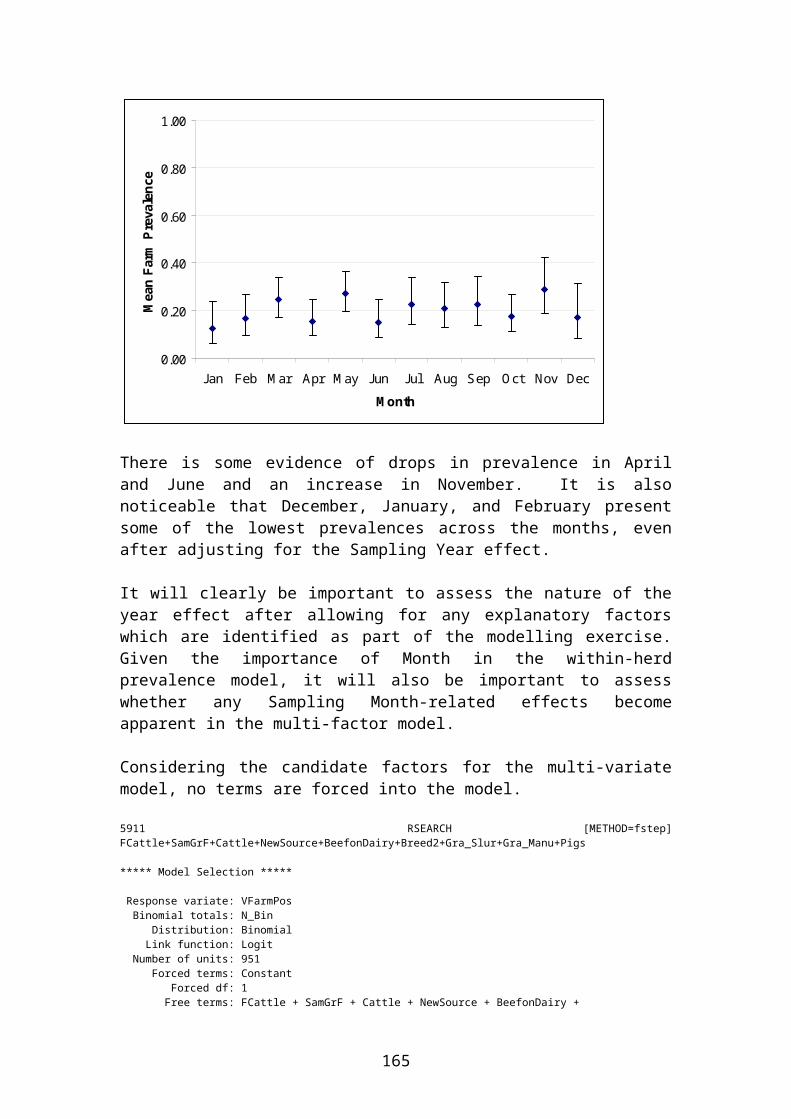
As seen in the earlier univariate analysis, there is clearly no evidence of any systematic effect due to Management Class.
Given the evidence for trend in the data with respect to Sampling Year, and our continued interest in Sampling Month, the first model to investigate temporal trend will fit a separate effect for each of the 27 months of the study:
5661 GLMM [PRINT=model,monitor,components,vcovariance,means,backmeans,effects; DISTRIBUTION=binomial;\5662 LINK=logit; DISPERSION=1; FIXED=SamGrF + Gra_Slur + Gra_Manu+BeefonDairy + Pigs + FCattle + Max_Age+Month;\5663 RANDOM=Farm; CONSTANT=estimate; FACT=9; PTERMS=Month; PSE=*; MAXCYCLE=20; FMETHOD=all;\5664 CADJUST=mean] VFarmPos; NBINOMIAL=N_Bin; MEANS=Means; VARMEANS=Vars ***** Generalised Linear Mixed Model Analysis ***** Method: cf Schall (1991) Biometrika Response variate: VFarmPos Distribution: BINOMIAL Link function: LOGIT Random model: Farm Fixed model: Constant + ((((((SamGrF + Gra_Slur) + Gra_Manu) + BeefinDairy) + Pigs) + FCattle) + Max_Age) + Month * Dispersion parameter fixed at value 1.000 ******** Warning from GLMM: missing values generated in weights/working variate. *** Monitoring information *** Iteration Gammas Dispersion Max change 1 0.2879 1.000 3.2307E+00 ******** Warning from GLMM: missing values generated in weights/working variate. 2 0.000001000 1.000 2.8787E-01 ******** Warning from GLMM: missing values generated in weights/working variate. 3 0.06742 1.000 6.7416E-02 ******** Warning from GLMM: missing values generated in weights/working variate. 4 0.2668 1.000 1.9935E-01 ******** Warning from GLMM: missing values generated in weights/working variate. 5 0.2801 1.000 1.3329E-02 ******** Warning from GLMM: missing values generated in weights/working variate. 6 0.2854 1.000 5.3309E-03 ******** Warning from GLMM: missing values generated in weights/working variate. 7 0.2862 1.000 7.9267E-04 ******** Warning from GLMM: missing values generated in weights/working variate. 8 0.2863 1.000 6.5874E-05
165

*** Estimated Variance Components *** Random term Component S.e. Farm 0.286 0.310 *** Residual variance model *** Term Factor Model(order) Parameter Estimate S.e. Dispersn Identity Sigma2 1.000 FIXED *** Estimated Variance matrix for Variance Components *** Farm 1 0.09603 Dispersn 2 0.00000 0.00000 1 2 *** Table of effects for Month *** Month 3.00 4.00 5.00 6.00 7.00 8.00 9.00 10.00 0.000 1.220 1.004 0.507 0.903 1.066 0.838 0.184 Month 11.00 12.00 13.00 14.00 15.00 16.00 17.00 18.00 1.334 0.567 -1.054 0.134 0.119 -0.460 0.852 -0.192 Month 19.00 20.00 21.00 22.00 23.00 24.00 25.00 26.00 0.916 0.367 1.638 0.304 0.049 -9.310 -0.455 -1.563 Month 27.00 28.00 29.00 0.272 -1.353 0.461 Standard error of differences: Average 3.266 Maximum 34.94 Minimum 0.4839 Average variance of differences: 90.87 *** Tables of means *** *** Table of predicted means for Month *** Month 3.00 4.00 5.00 6.00 7.00 -0.1603 1.0599 0.8437 0.3464 0.7428 Month 8.00 9.00 10.00 11.00 12.00 0.9057 0.6782 0.0238 1.1738 0.4065 Month 13.00 14.00 15.00 16.00 17.00 -1.2148 -0.0262 -0.0415 -0.6201 0.6913 Month 18.00 19.00 20.00 21.00 22.00 -0.3520 0.7553 0.2069 1.4780 0.1441 Month 23.00 24.00 25.00 26.00 27.00 -0.1110 -9.4700 -0.6156 -1.7231 0.1118 Month 28.00 29.00 -1.5135 0.3006
166

*** Back-transformed Means (on the original scale) *** Month 3.00 0.4600 4.00 0.7427 5.00 0.6992 6.00 0.5857 7.00 0.6776 8.00 0.7121 9.00 0.6633 10.00 0.5059 11.00 0.7638 12.00 0.6002 13.00 0.2289 14.00 0.4934 15.00 0.4896 16.00 0.3498 17.00 0.6663 18.00 0.4129 19.00 0.6803 20.00 0.5515 21.00 0.8143 22.00 0.5360 23.00 0.4723 24.00 0.0001 25.00 0.3508 26.00 0.1515 27.00 0.5279 28.00 0.1804 29.00 0.5746 Note: means are probabilities not expected values. 5666 VDISPLAY [PRINT=Wald] *** Wald tests for fixed effects *** Fixed term Wald statistic d.f. Wald/d.f. Chi-sq prob * Sequentially adding terms to fixed model SamGrF 19.74 3 6.58 <0.001 Gra_Slur 8.08 2 4.04 0.018 Gra_Manu 7.51 1 7.51 0.006 BeefonDairy 5.57 1 5.57 0.018 Pigs 3.52 1 3.52 0.060 FCattle 5.77 3 1.92 0.123 Max_Age 3.11 1 3.11 0.078 Month 45.97 26 1.77 0.009 * Dropping individual terms from full fixed model SamGrF 17.97 3 5.99 <0.001 Gra_Slur 16.57 2 8.29 <0.001 Gra_Manu 9.35 1 9.35 0.002 BeefonDairy 8.72 1 8.72 0.003 Pigs 6.65 1 6.65 0.010 FCattle 11.47 3 3.82 0.009 Max_Age 7.83 1 7.83 0.005 Month 45.97 26 1.77 0.009
Clearly, the month in which farms were sampled has a highly significant effect on the probability of a farm being identified as positive, even after allowing for the explanatory variables. The plot of mean prevalences by sampling month is as follows:
167

0
0.2
0.4
0.6
0.8
1
Mar-98
May-98
Jul-9
8
Sep-9
8
Nov-98
Jan-9
9
Mar-99
May-99
Jul-9
9
Sep-9
9
Nov-99
Jan-0
0
Mar-00
May-00
Month
Mea
n Fa
rm P
reva
lenc
e
There is a clear visual downwards trend in prevalence as the survey progressed, along with a seasonal effect which is slightly apparent in the 1998 data, is very apparent in the 1999 data, and which seems likely to be present in the 2000 data. In addition, there are peculiarities in the pattern of observed prevalences. In each of 1998 and 1999, there is evidence of an appreciable drop in prevalence in June, and in each of 1999 and 2000, there is evidence of an appreciable drop in prevalence in April. It is possible to overemphasise such apparent correlations in time series data, but it is reasonable to assume that the observed prevalence could change according to month, in line with changes in herd management and diet.
Fitting Sampling Month at this level of detail does not help to define a picture of any seasonal effects on the prevalence. Any model with which it is hoped to achieve this objective must allow for the long term drop in prevalence and the month-to month variability. The simplest appropriate model is felt to be one which fits both Sampling Year and Month of Sample as fixed effects. It will not be possible to fit an interaction term. Since the data were collected in random clusters by week within Animal Health Division, it is theoretically possible that some of the drops and peaks might be associated with the particular Divisions which were sampled during that month. This is unlikely, given the lack of significance seen earlier for Animal Health Division as a factor, but to test for this, the model is refitted also including Animal Health Division:
5677 VDISPLAY [PRINT=Wald] *** Wald tests for fixed effects *** Fixed term Wald statistic d.f. Wald/d.f. Chi-sq prob * Sequentially adding terms to fixed model SamGrF 21.25 3 7.08 <0.001 Gra_Slur 7.85 2 3.93 0.020 Gra_Manu 7.70 1 7.70 0.006 BeefonDairy 6.45 1 6.45 0.011 Pigs 4.14 1 4.14 0.042
168
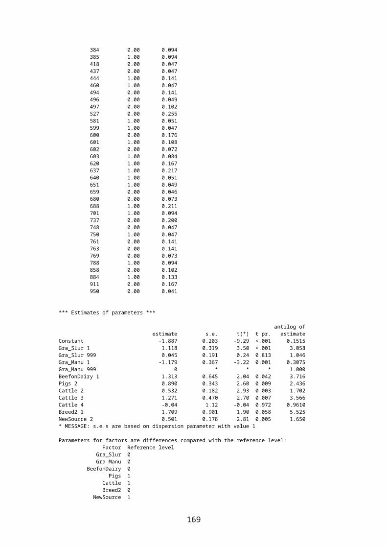
FCattle 5.99 3 2.00 0.112 Max_Age 3.15 1 3.15 0.076 Division 4.51 5 0.90 0.479 Sam_Year 14.19 2 7.09 <0.001 Sam_Mon 20.54 11 1.87 0.038 * Dropping individual terms from full fixed model SamGrF 16.92 3 5.64 <0.001 Gra_Slur 16.91 2 8.46 <0.001 Gra_Manu 9.36 1 9.36 0.002 BeefonDairy 10.55 1 10.55 0.001 Pigs 6.98 1 6.98 0.008 FCattle 10.04 3 3.35 0.018 Max_Age 7.19 1 7.19 0.007 Division 4.28 5 0.86 0.510 Sam_Year 6.91 2 3.45 0.032 Sam_Mon 20.54 11 1.87 0.038
The summarised results show that Division is insignificant as an effect, while Sampling Month is still significant. Hence, the model is refitted without this extraneous variable:
5684 GLMM [PRINT=model,monitor,components,vcovariance,means,backmeans,effects; DISTRIBUTION=binomial;\5685 LINK=logit; DISPERSION=1; FIXED=SamGrF + Gra_Slur + Gra_Manu+BeefonDairy + Pigs + FCattle + Max_Age+Sam_Year+Sam_Mon;\5686 RANDOM=Farm; CONSTANT=estimate; FACT=9; PSE=*; MAXCYCLE=20; FMETHOD=all; CADJUST=mean]\5687 VFarmPos; NBINOMIAL=N_Bin ***** Generalised Linear Mixed Model Analysis ***** Method: cf Schall (1991) Biometrika Response variate: VFarmPos Distribution: BINOMIAL Link function: LOGIT Random model: Farm Fixed model: Constant + (((((((SamGrF + Gra_Slur) + Gra_Manu) + BeefinDairy) + Pigs) + FCattle) + Max_Age) + Sam_Year) + Sam_Mon * Dispersion parameter fixed at value 1.000 ******** Warning from GLMM: missing values generated in weights/working variate. *** Monitoring information *** Iteration Gammas Dispersion Max change 1 0.1777 1.000 3.3648E+00 ******** Warning from GLMM: missing values generated in weights/working variate. 2 0.000001000 1.000 1.7774E-01 ******** Warning from GLMM: missing values generated in weights/working variate. 3 0.000001000 1.000 0.0000E+00 *** Estimated Variance Components *** Random term Component S.e. Farm 0.000 0.283 *** Residual variance model *** Term Factor Model(order) Parameter Estimate S.e.
169

Dispersn Identity Sigma2 1.000 FIXED *** Estimated Variance matrix for Variance Components *** Farm 1 0.07987 Dispersn 2 0.00000 0.00000 1 2 *** Table of effects for Constant *** -3.180 Standard error: 0.5414 *** Table of effects for SamGrF *** SamGrF 1 2 3 4 0.0000 0.8074 0.7204 1.1645 Standard error of differences: Average 0.2488 Maximum 0.2693 Minimum 0.2278 Average variance of differences: 0.06224 *** Table of effects for Gra_Slur *** Gra_Slur 0.0 1.0 999.0 0.0000 1.3087 0.6259 Standard error of differences: Average 0.3242 Maximum 0.3755 Minimum 0.2704 Average variance of differences: 0.1069 *** Table of effects for Gra_Manu *** Gra_Manu 0.0 1.0 999.0 0.0000 -1.1917 0.0000 Standard error of differences: 0.3676 *** Table of effects for BeefonDairy *** BeefonDairy 0.0000 1.0000 0.000 2.206 Standard error of differences: 0.6646 *** Table of effects for Pigs *** Pigs 1 2 0.0000 1.0280 Standard error of differences: 0.3655 *** Table of effects for FCattle *** FCattle 1 2 3 4 0.0000 0.3878 0.3844 1.1158 Standard error of differences: Average 0.2810
170

Maximum 0.3371 Minimum 0.2135 Average variance of differences: 0.08154 *** Table of effects for Max_Age *** -0.04357 Standard error: 0.016086 *** Table of effects for Sam_Year *** Sam_Year 1998 1999 2000 0.0000 -0.4249 -0.7956 Standard error of differences: Average 0.2577 Maximum 0.3071 Minimum 0.2076 Average variance of differences: 0.06806 *** Table of effects for Sam_Mon *** Sam_Mon Jan Feb Mar Apr May Jun Jul Aug 0.0000 0.1722 0.8812 0.2479 1.2634 0.4584 1.1696 1.0222 Sam_Mon Sep Oct Nov Dec 1.2757 0.5800 1.1474 0.2218 Standard error of differences: Average 0.4615 Maximum 0.5939 Minimum 0.3495 Average variance of differences: 0.2163 **** G5W0020 **** Warning (Code VC 19). Statement 268 in Procedure GLMM Command: VKEEP #PFORM; MEANS=MEANS[]; VARMEANS=VARMEANS[]Table/sed matrix not available for mean effects of covariates Table of mean effects cannot be saved for term Max_Ageas it is a variate/covariate *** Tables of means *** * Using covariate mean values *** Table of predicted means for SamGrF *** SamGrF 1 2 3 4 -0.5474 0.2600 0.1730 0.6171 *** Table of predicted means for Gra_Slur *** Gra_Slur 0.0 1.0 999.0 -0.5192 0.7895 0.1067 *** Table of predicted means for Gra_Manu *** Gra_Manu 0.0 1.0 999.0 0.5229 -0.6688 0.5229
171

*** Table of predicted means for BeefonDairy *** BeefonDairy 0.0000 1.0000 -0.977 1.228 *** Table of predicted means for Pigs *** Pigs 1 2 -0.3883 0.6397 *** Table of predicted means for FCattle *** FCattle 1 2 3 4 -0.3463 0.0415 0.0381 0.7694 *** Table of predicted means for Sam_Year *** Sam_Year 1998 1999 2000 0.5325 0.1076 -0.2630 *** Table of predicted means for Sam_Mon *** Sam_Mon Jan Feb Mar Apr May -0.5776 -0.4054 0.3036 -0.3298 0.6857 Sam_Mon Jun Jul Aug Sep Oct -0.1192 0.5920 0.4446 0.6980 0.0023 Sam_Mon Nov Dec 0.5698 -0.3558 *** Back-transformed Means (on the original scale) *** * Using covariate mean values SamGrF 1 0.3665 2 0.5646 3 0.5431 4 0.6496 Gra_Slur 0.0 0.3730 1.0 0.6877 999.0 0.5267 Gra_Manu 0.0 0.6278 1.0 0.3388 999.0 0.6278 BeefonDairy 0.0000 0.2735 1.0000 0.7736 Pigs 1 0.4041 2 0.6547 FCattle 1 0.4143
172

2 0.5104 3 0.5095 4 0.6834 Sam_Year 1998 0.6301 1999 0.5269 2000 0.4346 Sam_Mon Jan 0.3595 Feb 0.4000 Mar 0.5753 Apr 0.4183 May 0.6650 Jun 0.4702 Jul 0.6438 Aug 0.6094 Sep 0.6678 Oct 0.5006 Nov 0.6387 Dec 0.4120 Note: means are probabilities not expected values. 5688 VDISPLAY [PRINT=Wald] *** Wald tests for fixed effects *** Fixed term Wald statistic d.f. Wald/d.f. Chi-sq prob * Sequentially adding terms to fixed model SamGrF 23.99 3 8.00 <0.001 Gra_Slur 8.78 2 4.39 0.012 Gra_Manu 8.64 1 8.64 0.003 BeefonDairy 6.90 1 6.90 0.009 Pigs 4.40 1 4.40 0.036 FCattle 6.56 3 2.19 0.087 Max_Age 3.47 1 3.47 0.063 Sam_Year 16.00 2 8.00 <0.001 Sam_Mon 22.04 11 2.00 0.024 * Dropping individual terms from full fixed model SamGrF 19.06 3 6.35 <0.001 Gra_Slur 18.22 2 9.11 <0.001 Gra_Manu 10.51 1 10.51 0.001 BeefonDairy 11.01 1 11.01 <0.001 Pigs 7.91 1 7.91 0.005 FCattle 11.86 3 3.95 0.008 Max_Age 7.33 1 7.33 0.007 Sam_Year 7.25 2 3.63 0.027 Sam_Mon 22.04 11 2.00 0.024
Both Month and Year of Sampling are found to have a statistically significant influence on the probability of a farm being classed as positive for shedding. The inclusion of these structural variables has a negligible effect on the significances estimated for the explanatory factors.
Reviewing the effect of Sampling Year, the estimated mean prevalences for the three years of the study, adjusted for Sampling Month effects and all the explanatory factors, are:
Year Mean Farm Prevalence1998 0.63
173

1999 0.532000 0.43
Plotting the mean prevalence with the associated 95% confidence intervals gives:
0.00
0.20
0.40
0.60
0.80
1.00
1998 1999 2000
Year
Mea
n Fa
rm P
reva
lenc
e
The nature of the trend is clear. There is a year on year drop in prevalence, which is statistically significant overall (p=0.03). The drop from 1998 to 1999 exhibits a mean change of –0.425, with a standard error of 0.208. The associated t-statistic equals 2.05, with a p-value of 0.04. The drop from 1999 to 2000 is not statistically significant (change=-0.37, se=0.26, t=1.44, p=0.15). The nature of the trend is identical to that seen in the analysis involving only year and month, but the estimated effects are much more significant for 1998/1999, presumably since much of the extraneous noise in the initial analysis has been explained by the explanatory variables in the multi-factor model, and less significant for 1999/2000, presumably since much of the effect in 2000 has been explained by other explanatory factors which were strongly unbalanced in the (abbreviated) sampling year 2000.
Reviewing the effect of Sampling Month, the estimated mean prevalences for the each month of the year, adjusted for Sampling Year effects and all the explanatory factors, are:
MonthMean Farm Prevalence
Jan 0.36Feb 0.40Mar 0.58Apr 0.42May 0.67Jun 0.47Jul 0.64
Aug 0.61
174

Sep 0.67Oct 0.50Nov 0.64Dec 0.41
A more clear picture is provided by plotting the mean prevalence with the associated 95% confidence intervals, giving:
0.00
0.20
0.40
0.60
0.80
1.00
Jan Feb Mar Apr May Jun Jul Aug Sep Oct Nov Dec
Month of Sampling
Mea
n Fa
rm P
reva
lenc
e
There appears to be a clear seasonal cycle in prevalence, with higher values in late Sprint and Summer, and lower values in December to February. However, over and above this, there is evidence of other monthly effects occurring against the cycle, perhaps most blatantly in June, and probably in March, April and November. Again, the nature of the month to month effect is unchanged relative to the initial analysis involving only month and year, but the estimated effects exhibit a greater significance, presumably due to the greater explanatory value of the multi-factor model.
It is tempting to consider that, previous evidence notwithstanding, the Sampling Month effect might be associated with Housing status, as was the within-farm prevalence on positive farms. To test this hypothesis, the model is refitted, including Housed as a further explanatory factor. The (summarised) results are as follows:
5730 VDISPLAY [PRINT=Wald] *** Wald tests for fixed effects *** Fixed term Wald statistic d.f. Wald/d.f. Chi-sq prob * Sequentially adding terms to fixed model SamGrF 24.20 3 8.07 <0.001 Gra_Slur 8.46 2 4.23 0.015 Gra_Manu 8.77 1 8.77 0.003 BeefonDairy 6.90 1 6.90 0.009
175

Pigs 4.37 1 4.37 0.037 FCattle 6.40 3 2.13 0.094 Max_Age 3.45 1 3.45 0.063 Sam_Year 15.98 2 7.99 <0.001 Housed 0.55 1 0.55 0.460 Sam_Mon 21.94 11 1.99 0.025 * Dropping individual terms from full fixed model SamGrF 19.25 3 6.42 <0.001 Gra_Slur 16.54 2 8.27 <0.001 Gra_Manu 10.65 1 10.65 0.001 BeefonDairy 11.02 1 11.02 <0.001 Pigs 7.87 1 7.87 0.005 FCattle 11.64 3 3.88 0.009 Max_Age 7.24 1 7.24 0.007 Sam_Year 7.32 2 3.66 0.026 Housed 0.53 1 0.53 0.467 Sam_Mon 21.94 11 1.99 0.025
Housed remains completely insignificant as an explanatory factor, and Sampling Month and Sampling Year are unchanged in terms of overall significance levels.
Hence, there is clear evidence of a temporal structure in the data, both over the long term (a significant decrease in the proportion of farms detected as positive over the lifetime of the project), and over the short term (a significant month to month variability, unexplained by the explanatory variables fitted in the multi-factor model).
176

Appendix 1: Variates and Factors Collected by the Farm Questionnaire.
Factor/Variable Comments LevelsManage_O Observed management type. Beef, Dairy, Other, MixedDivision Animal Health Division, with one division divided into Highlands and Islands. Central, Highlands, Islands, NE, SE, SWSam_Month Month in which samples were collected. January-DecemberSample Type of sampling scheme. Faecal Pat, RectalSam_Year Year in which samples were collected. 1998, 1999, 2000
Sampler Person carrying out sampling. H, F (codes)N_F_Cattle Number of finishing cattle on farm. VariateFCattle Number of finishing cattle, categorised into groups. <50, 50-99, 100-199, 200+N_Groups Number of management groups of cattle on farm. VariateGroupsCat Number of management groups, categorised into groups. 1, 2-5, 6-9, 10+N_Sam_Gr Number of finishing cattle in sampling group. VariateMin_Age Minimum age of animals in sampling group. VariateMax_Age Maximum age of animals in sampling group. VariateSource Farm policy for replacement cattle. Buy In, Breeding Only, BothNewSource Restructuring of 'Source' into open and closed farms. Open, Closed
Breed Breed of cattle in sampling group.Beef (Suckler Beef), Dairy Beef, Dairy (Bull Beef), Combinations of these
Housed Whether sampling group are housed or unhoused. Housed, UnhousedHousing For housed animals only: type of housing. Court/Straw Yard, Slats, Byre, OtherTDHouse Number of months for which animals have been in current housed state. Variate
Rec_MoveWhether or not the sampling group have been moved in the 4 weeks prior to sampling. Yes, No
SupFeed For unhoused animals only: whether the sampling group is fed supplements. Yes, No
RecDFeedWhether or not the sampling group have had a change in diet in the 4 weeks prior to sampling. Yes, No
Forage For housed animals only: whether the sampling group is fed forage. Yes, NoSilage For housed animals only: whether the sampling group is fed silage. Yes, NoConcentrate For housed animals only: whether the sampling group is fed concentrate. Yes, NoSil_Home For housed animals fed silage only: whether the farm produces silage. Yes, No
Sil_ManureFor housed animals fed farm-produced silage only: whether the farm spreads manure on the silage fields. Yes, No
Sil_SlurryFor housed animals fed farm-produced silage only: whether the farm spreads slurry on the silage fields. Yes, No
Sil_SewageFor housed animals fed farm-produced silage only: whether the farm spreads sewage on the silage fields. Yes, No
Sil_GeeceFor housed animals fed farm-produced silage only: whether geese have been observed on the silage fields. Yes, No
Sil_GullsFor housed animals fed farm-produced silage only: whether gulls have been observed on the silage fields. Yes, No
Hay Whether the farm produces hay. Yes, No
Hay_ManureIf the farm produces hay only: whether the farm spreads manure on the hay fields. Yes, No
Hay_Slurry If the farm produces hay only: whether the farm spreads slurry on the hay fields. Yes, No
Hay_SewageIf the farm produces hay only: whether the farm spreads sewage on the hay fields. Yes, No
Hay_GeeseIf the farm produces hay only: whether geese have been observed on the hay fields. Yes, No
Hay_GullsIf the farm produces hay only: whether gulls have been observed on the hay fields. Yes, No
Grass_Manure Whether the farm spreads manure on pasture. Yes, NoGrass_Slurry Whether the farm spreads slurry on pasture. Yes, NoGrass_Sewage Whether the farm spreads sewage on pasture. Yes, NoGrass_Geece Whether geese have been observed on pasture. Yes, NoGrass_Gulls Whether gulls have been observed on pasture. Yes, NoN_Cattle Number of cattle on farm other than the finishing group. Variate
CattleNumber of cattle on farm other than the finishing group, categorised into a factor. <100, 100-499, 500-899, 900+
N_Sheep Number of sheep on farm. VariateSheep Absence/presence of sheep on farm. Yes, NoN_Goats Number of goats on farm. VariateGoats Absence/presence of goats on farm. Yes, NoN_Horses Number of horses on farm. VariateN_Pigs Number of pigs on farm. VariatePigs Absence/presence of pigs on farm. Yes, No
177

N_Chickens Number of chickens on farm. VariateChickens Absence/presence of chickens on farm. Yes, NoN_Deer Number of deer on farm. VariateDeer Absence/presence of deer on farm. Yes, NoMains Whether sampling group is watered with a mains supply. Yes, NoPrivate Whether sampling group is watered with a private supply. Yes, NoNatural Whether sampling group is watered with a natural supply. Yes, NoWaterCon Whether water have been contaminated within the 12 months prior to sampling. Yes, No
WaterCT Possible sources of contamination.Animals Upstream, Septic Tank, Midden, Combinations of these
Want2Know Whether farmer wishes to know results of sampling. Yes, NoVisit2 Whether farmer is willing to have a further set of samples collected. Yes, NoLabOperator Lab operator responsible for assaying faeces samples. S, D, H (codes)BeefonDairy Whether farm is classed as a dairy farm with suckler beef cattle. Yes, No
178