Analysing Debris-Flow Impact Models, Based on a SmallScale Modelling Approach

Christian Scheidl • Michael Chiari • Roland Kaitna • Matthias Mullegger •

Alexander Krawtschuk • Thomas Zimmermann • Dirk Proske

Received: 8 December 2011 / Accepted: 27 June 2012 / Published online: 18 July 2012� The Author(s) 2012. This article is published with open access at Springerlink.com

Abstract The objective of this study is to analyse adaptable debris-flow impact models,

which are very important for mitigation measurements and buildings using their sphere of

influence. For this reason, 16 debris-flow experiments, on a small-scale modelling approach,

were performed. Impact forces were measured with a force plate panel, consisting of 24

aluminium devices, coaxially mounted with resistance strain gauges. Flow velocities, flow

heights as well as horizontal impact forces were sampled with a frequency of 2.4 kHz. Sub

datasets of sampled raw force data were defined by applying an average median filter, a low-

pass filter routine. Further, estimated peak pressure values as well as empirical coefficients of

hydraulic impact models were compared, and the influence of signal processing is discussed.

Keywords Debris flow � Impact force � Physical modelling � Signal processing

1 Introduction

Debris flows endanger human living in mountainous regions all over the world. The design

of structural mitigation measures, like debris-flow barriers, or the maintenance of infra-

structures such as bridges, requires the estimation of potential impact forces caused by

debris flows. Currently, no entirely mechanistically and theoretically based impact model

is sufficiently accurate and computable in periods common for design offices (Proske et al.

2008; Hubl et al. 2009). Debris-flow impact models for engineering purposes are, there-

fore, mainly based on rational arguments and empirical approaches, as stated for instance

by Egli (2005) or the Austrian code series ONR2480X; the latter is currently under

C. Scheidl (&) � M. Chiari � R. Kaitna � M. Mullegger � D. ProskeInstitute of Mountain Risk Engineering, University of Natural Resources and Life Sciences, Vienna,Peter-Jordan-Strasse 82, 1190 Wien, Austriae-mail: christian.scheidl@boku.ac.at

A. Krawtschuk � T. ZimmermannInstitute of Structural Engineering, University of Natural Resources and Life Sciences, Vienna,Wien, Austria

123

Surv Geophys (2013) 34:121–140DOI 10.1007/s10712-012-9199-6

development. Wendeler (2008) analysed existing debris-flow impact models and their

adaptability to design flexible debris-flow barriers.

Impact forces caused by real-scale debris-flow events have been measured at Mt. Yake-

dake in Japan (Okuda et al. 1977), in the Jiangjia Ravine in China (Zhang 1993; Hu et al.

2011), at the Schesatobel in Austria (Konig 2006) and in the Illgraben torrent in Switzerland

(Wendeler et al. 2007). An example of a large scale experiment is given by DeNatale et al.

(1999) and Bugnion et al. (2011). The advantage of large scale debris-flow experiments or

impact force measurements of natural debris flows at monitoring stations is that scaling

considerations with regard to the process are not necessary. However, the possibility to gather

systematic data for controlled boundary conditions is limited. For instance, the unknown

frequency of occurrence of a debris-flow event and therewith the effort of the installation and

operation of measurement devices are main disadvantages of real-scale observations. And for

large scale experiments, the expected volume of the event makes the design of the mea-

surement setup cost-intensive and flow and material parameters are often unknown.

For this reasons, laboratory small scale experiments (measuring debris-flow impacts)

have also been carried out, accepting the difficulty in scaling debris flows for physical

modelling (Armanini and Scotton 1992; Ishikawa et al. 2008; Hubl and Holzinger 2003;

Tiberghien et al. 2007; Monney et al. 2007; Shieh et al. 2008; Wendeler 2008). Due to the

complex flow behaviour of debris flows including scale dependent interactions between the

solid and the fluid phase (Iverson and Denlinger 2001; Iverson et al. 2011), a common

approach to extrapolate from experimental scale to field scale is often based on hydro-

dynamic approaches, assuming geometric as well as simple kinematic similarity. This

seems to be justified, since these experiments focus on the impacts of sediment-fluid

mixtures on an obstacle rather than on the flow dynamics of debris flows. Kinematic

similarity is characterised by the dimensionless Froude number (Fr), which is the ratio of

inertial and gravitational forces of the flowing mass. For this approach, the Froude number

should have values similar to natural debris-flow events. Hubl et al. (2009) showed that the

impact forces of the real-scale observations have mainly been estimated in a Froude range

between 0 and 2, but only the tests by Tiberghien et al. (2007) reach this range. Minia-

turised tests were mainly carried out at higher Froude numbers, concluding that models

based on these experimental data do not comply with field data

The objective of this study is to analyse impact forces of granular and viscous debris

flows based on small scale laboratory experiments. All tests rely on Froude scaling,

accomplished with Froude numbers, Fr \ 3. After an overview of existing debris-flow

impact models, a detailed description of the laboratory flume as well as the experimental

setup is given. Measured peak flow heights, maximum velocities, and peak pressure values

are presented. The measurements are compared to existing impact models, especially to the

modified hydrodynamic model of Hubl and Holzinger (2003), which is strongly related to

the Austrian code series ONR2480X currently under development. Finally, observations of

single, short time impacts of large particles, significantly exceeding the peak pressure

values, are discussed.

2 Debris-Flow Impact Models

Debris-flow impact models suggested for the design of engineering structures can be

classified into hydraulic and solid-collision models (Hubl et al. 2009). This twofold

classification reflects the complexity of debris-flow processes, where the impact can either

be caused by fluid-phase slurry thrusting or a point-wise loading due to coarse solid

122 Surv Geophys (2013) 34:121–140

123

particle collision (Hu et al. 2011). These solid body impact models assume elastic material

behaviour and are mainly based on the Hertz model. Alternative models, considering

viscous-elastic and elastic-plastic behaviour, are proposed by Walton and Braun (1986)

and Thornton (1997). This study focuses on hydraulic models, which can be separated into

hydrostatic and hydrodynamic models.

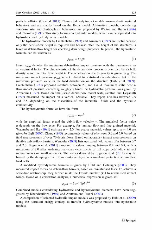
The hydrostatic models by Lichtenhahn (1973) and Armanini (1997) are useful because

only the debris-flow height is required and because often the height of the structures is

taken as debris-flow height for checking dam design purposes. In general, the hydrostatic

formula can be written as:

ppeak ¼ kqgh ð1Þ

Here, ppeak denotes the maximum debris-flow impact pressure with the parameter k as

an empirical factor. The characteristic of the debris-flow process is described by its bulk

density q and the total flow height h. The acceleration due to gravity is given by g. The

maximum impact pressure ppeak is not related to statistical considerations, but to the

maximum pressure value in the load distribution on the structure (Hubl et al. 2009).

Lichtenhahn (1973) proposed k-values between 2.8 and 4.4. A maximum static debris-

flow impact pressure, exceeding roughly 5 times the hydrostatic pressure, was given by

Armanini (1997). Based on small-scale debris-flow model tests, Scotton and Deganutti

(1997) measured the impact on a vertical obstacle. They report k-values between 2.5

and 7.5, depending on the viscosities of the interstitial fluids and the hydraulic

conductivity.

The hydrodynamic formulas have the form

ppeak ¼ aqv2 ð2Þ

with the empirical factor a and the debris-flow velocity v. The empirical factor value

a depends on the flow type. For example, for laminar flow and fine grained material,

Watanabe and Ike (1981) estimate a = 2.0. For coarse material, values up to a = 4.0 are

given by Egli (2005). Zhang (1993) recommends values of a between 3.0 and 5.0, based on

field measurements of over 70 debris flows. Based on laboratory impact measurements on

flexible debris-flow barriers, Wendeler (2008) lists up scaled field values of a between 0.7

and 2.0. Bugnion et al. (2011) proposed a values ranging between 0.4 and 0.8, with a

maximum of 2.0 after analysing real-scale experiments of hill slope debris-flow impact

measurements on small obstacles. The values denoted by Bugnion et al. (2011) may be

biased by the damping effect of an elastomer layer as a overload protection within their

load cells.

A modified hydrodynamic formula is given by Hubl and Holzinger (2003). They

measured impact forces on debris-flow barriers, based on miniaturised tests. To achieve a

scale-free relationship, they further relate the Froude number (Fr) to normalised impact

forces. Based on a correlation analysis, a numerical expression is given as:

ppeak ¼ 5qv0:8ðghÞ0:6 ð3Þ

Combined models considering hydrostatic and hydrodynamic elements have been sug-

gested by Kherkheulidze (1969) and Arattano and Franzi (2003).

A comparison of selected hydraulic impact models was proposed by Hubl et al. (2009)

using the Bernoulli energy concept to transfer hydrodynamic models into hydrostatic

models:

Surv Geophys (2013) 34:121–140 123

123

kqgh ¼ aqv2

2ð4Þ

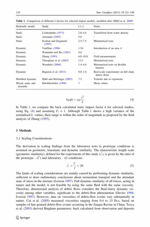
In Table 1, we compare the back calculated static impact factor k for selected studies,

using Eq. (4) and assuming Fr = 1. Although Table 1 shows a high variance of the

normalised k -values, their range is within the order of magnitude as proposed by the field

analysis of Zhang (1993).

3 Methods

3.1 Scaling Considerations

The derivation in scaling findings from the laboratory tests to prototype conditions is

assumed on geometric, kinematic and dynamic similarity. The characteristic length scale

(geometric similarity), defined for the experiments of this study (k0), is given by the ratio of

the prototype - (l*) and laboratory - (l) conditions:

k0 ¼ l�

l¼ 20 ð5Þ

The limits of scaling considerations are mainly caused by performing dynamic similarity,

sufficient to draw rudimentary conclusions about momentum transport and the attendant

state of stress in the mixture (Iverson 1997). Full dynamic similarity of all forces, acting in

nature and the model, is not feasible by using the same fluid with the same viscosity.

Therefore, dimensional analysis of debris flows considers the fluid-slurry dynamic vis-

cosity among other variables, significant to the debris-flow phenomenon (Davies 1994;

Iverson 1997). However, data on viscosities of debris-flow events vary substantially in

nature. Cui et al. (2005) measured viscosities ranging from 0.4 to 15 Pa.s, based on

samples of fine grained debris-flow events occurring in the Jiangia Ravine in China. Tecca

et al. (2003) derived Bingham parameters, back calculated from observation and deposits

Table 1 Comparison of different k factors for selected impact models, modified after (Hubl et al. 2009)

Hydraulic model Study k [–] Notes

Static Lichtenhahn (1973) 2.8–4.4 Transferred from water density

Static Armanini (1997) 5.0 -

Static Scotton and Deganutti(1997)

2.5–7.5 Miniaturised tests

Dynamic VanDine (1996) 1.5A Introduction of an area A

Dynamic Watanabe and Ike (1981) 4.0 -

Dynamic Zhang (1993) 6.0–10.0 Field measurements

Dynamic Tiberghien et al. (2007) 13.5 Miniaturised tests

Dynamic Wendeler (2008) 1.4–4.0 Miniaturised tests on flexiblebarriers

Dynamic Bugnion et al. (2011) 0.8–1.6 Real-scale experiments on hill slopedebris flows

Modified dynamic Hubl and Holzinger (2003) 7.5 Transfer due to exponents

Mixed, static anddynamic

Kherkheulidze (1969) 1 Mean values

124 Surv Geophys (2013) 34:121–140

123

of granular debris-flow events. They report viscosities ranging from 5 to 75 Pa.s, varying

by a factor of five compared to the measurements of the muddy debris flows of the Jiangia

Ravine. We, therefore, defined two different bulk mixtures for our experimental tests,

reflecting a more granular or viscous flow behaviour. Since viscosities of debris-flow

events have yet to be verified, we further decided to apply the Froude scaling concept to

our experimental test:

v�ffiffiffiffiffiffi

gl�p ¼ Fr ¼

vffiffiffiffi

glp ð6Þ

Here, v* and v refer, respectively, to the prototype and laboratory maximum surface

velocities at the debris-flow front. The gravitational attraction is denoted by g, whereas l*

as well as l denote the peak flow heights of the prototype and laboratory experiments,

respectively.

The prototype pressure values (p*) are then estimated, based on the measured pressure

values (p) by means of:

p� ¼ pk0 ð7Þ

In Table 2, selected laboratory and prototype parameters for this study, satisfying Froude

scaling and based on the characteristic length scale (Eq. 5), are compared.

3.2 Debris-Flow Material

The experimental bulk mixtures are based on water combined with a defined grain-size

distribution of solid particles, which may consist of loam (0.0002–0.1 mm) and bedload

sediments (0.1–50 mm). The dry mass of the particles was kept constant with 370 kg, and

only the water content remained variable. The maximum used grain diameter of 50 mm was

defined in accordance to the maximum flow width of the flume (450 mm), as well as to the

size of the impact area of each aluminium device (40 9 40 mm) within the force plate. The

total bulk density (qdf) was averaged to be 2,000 kg/m3. Figure 1 shows the grain-size

distribution used for this study compared to selected grain-size distributions for debris flows

based on field observations (VAW 1992; Hu et al. 2011). The grain-size distribution, used by

D’Agostino et al. (2010), refers to debris-flow material used in their laboratory tests. The

granular bulk mixture consisted only of particles with diameters larger than 0.1 mm. Here,

we substituted the finer particles with water to achieve a constant mass concentration.

The viscous mixture included fine particles consisting of 26 % clay, 60 % silt and 14 %

sand. The results of a mineral analysis showed 15 % of swellable Smektit within the clay

fraction, which counteracts phase seperation for a longer time period.

Table 2 Range of laboratory and prototype parameters for the experiments of this study

B[m] dmax [m] v [m/s] h [m] Fr [–] ppeak [kN/m2]

laboratory 0.45 0.05 0.6–2.5 0.06–0.16 0.7–3.2 0.28–1.02

prototype 9.00 1.00 2.8–10.9 1.20–3.20 0.7–3.2 5.66–20.31

Here, B denotes the flow width, whereas dmax refers to the maximum grain size. The maximum measuredvelocities and flow heights are denoted, respectively, by v and h. Fr refers to the related Froude number andppeak refers to the maximum debris-flow impact pressures (Eq. 1–3)

Surv Geophys (2013) 34:121–140 125

123

3.3 Experimental Device

The experiments were conducted at the Institute of Mountain Risk Engineering (IAN) at

the University of Natural Resources and Life Sciences, Vienna. The flume is made out of

wood and has a total length of 6.5 m. For this study, the slope of the flume remained fixed

at 30 % and had a constant flow width of 0.45 m (Fig. 2). Functionally, the construction

can be separated into a start (reservoir) and a measuring section (flume).

The start section is about 2 9 1 m in plan view and can hold a total volume of 0.33 m3,

which can be released with a simple start mechanism, imitating a dam-break scenario.

Figure 3a shows the start section with the starting mechanism at the moment of the release

of a viscous debris-flow experiment.The measuring section begins after the start section

and has in total a length of 4.5 m. The height of the side walls amounts to 0.5 m. Since the

flume slope remained constant, the roughness of the basal layer of the measuring section

was adapted to meet the desired Froude numbers. After several tests, an epoxy-sand

coating with a d50 of about 1 mm showed most suitable results.

The measuring devices are mounted along the measuring section and are comprised of

three ultrasonic devices, installed to measure flow heights at fixed lengths from the starting

mechanism (Fig. 3b) and one force plate panel, installed at the end of the flume, to measure

horizontal impact forces.

This force plate panel consists of 24 cuboidal aluminium devices, coaxially mounted

with resistance strain gauges (Fig. 4a). The impact area of each load cell has a quadratic

shape of 0.04 9 0.04 m, which results in a total impact area of the force plate panel of

0.0384 m2. In Fig. 4b, the frontal view (impact side) of the force panel, discretised due to

24 load cells, can be seen. Each load cell was individually calibrated in steps of 1 kN over

a range of 0 to 4 kN. The calibration was done by using a universal testing machine

(Fig. 4d). Size and situation of the load cells within the force plate is shown in Fig. 5.The

Fig. 1 Grain-size distribution of the debris-flow material used in this study, compared to selected grain-sizedistributions of observed events in Switzerland (VAW 1992), China (Hu et al. 2011) and used for laboratorytests by D’Agostino et al. (2010)

126 Surv Geophys (2013) 34:121–140

123

Fig. 2 Sketch of the experimental flume at the IAN-laboratory. All specifications are in mm

Fig. 3 a Start section and starting mechanism (steel plate) at the moment of a debris-flow release from topview. b Bottom view measuring section with the three ultrasonic devices US1, US2 and US3 (counting fromupstream), mounted in the middle of the channel

Surv Geophys (2013) 34:121–140 127

123

design of the force plate allows an installation on the orographic left side, or in the centre

of the flume, so that the flow was never completely stopped by the force plate. Addi-

tionally, three camera devices were installed, showing videos with a view from the starting

box, the force plate and the measuring section.

In total, 30 experiments were carried out, whereas the number of experiments was

limited due to the large amount of the total mass(&400 kg), which had to be mobilised.

Each experiment consisted of 370 kg solid particles, based on the defined grain-size dis-

tribution (Fig. 1), and combined with a certain amount of water. The slope of the flume as

well as the basal friction condition remained fixed for all experiments. The variability of

the flow dynamics of each experiment was therefore only controlled by the variability of

the added water content by weight. Thus, a low water content of the bulk mass resulted in

low Froude numbers. Minimum water contents per weight and Froude numbers were

observed for experiments with flow heights approximating to the maximum grain size of

Fig. 4 a Detailed view of the cuboidal aluminium devices to measure horizontal load forces based onresistance strain gauges. b Frontal view of the force plate panel, discretised due to 24 load cells. c Plan viewof the installed force plate panel, related to the flume construction. d Universal testing machine to calibratethe load cells individually

128 Surv Geophys (2013) 34:121–140

123

the solid particles (0.05 m). With increasing water content, we further observed an

increase in the turbulence of the bulk mixture and a decoupling of material and fluid.

Therefore, experiments of Fr [ 3 were excluded from further analysis. Table 3 gives an

overview of the selected experiments, the added water contents per weight and the esti-

mated maximum flow parameters. The variance of the measured maximum flow velocities

and flow heights, and Froude numbers, for identical experimental setups, are in a small

range. However, the deviation of the measured maximum velocities for each setup might

be explained due the relatively short measuring sector, which affects the development of a

full steady flow.

For each experiment, the impact forces of all load cells and the flow heights along the

flume were sampled over a certain time period. This time period varied for each experi-

ment since the opening of the starting mechanism and the start of the measuring devices

were not coincidental.

All measured data were sampled with a frequency of 2.4 kHz using a MGCplus data-

logger of the company HBM. The results were stored in ascii-file format.

3.4 Processing of the Impact Signal

Measurement of single impacts of short duration needs a sampling frequency sufficient to

capture the true peak force. In this study, we do not focus on these single impacts of very

short duration, but on the maximum bulk impact force over durations relevant for engi-

neering design purposes. However, since there is no critical duration of impacts on an

engineering structure, our data analysis compares different approaches.

For each experiment, 24 time series of force signals (based on the 24 load cells) were

sampled. All the scanned raw data were primarily filtered, regarding the Nyquist-Shannon

sampling theorem:

Fig. 5 Size and situation of theload cells forming the force plate.Each square represents one loadcell, starting with load cell Nr. 1in the lower left corner to loadcell Nr. 24 in the upper rightcorner

Surv Geophys (2013) 34:121–140 129

123

fscan [ 2fmax ð8Þ

Considering the applied scan frequency (fscan), Eq. 8 yields a refined dataset with a

maximum frequency (fmax) for data interpretation. Hence, the force signals, used for further

analysis, consist of sampled data within a frequency range between 0 and 1,190 Hz. This

dataset is referred to as the dataset of the entire signals (dataset A). Figure 6 shows forces

over time, based on dataset A of load cell 1 and experiment 1. Also shown is the median of

the entire signals based on a running window of 300 Hz, which is denoted as the dataset of

the average signals (dataset B). The window size was chosen as a best-fit parameter to

eliminate random effects but keeping the long-term response of the signal. Random effects

seemed to be based on the resonance frequency of the force plate and on single impacts of

very short duration. Certainly, dataset B also reduces the peak values of the force signals.

However, analysis showed that the random effects were measured in higher frequency

ranges. Dataset C is therefore defined as a low-pass filtered version of dataset A. The

related threshold frequency (maximum low pass frequency) is based on the following

theoretical considerations. Video observations showed that the total area of load cells,

which measured maximum forces over time, were always entirely hit by the experimental

debris-flow front. Assuming an experimental ‘‘debris’’ flow as a mono-phase flux, we

defined the maximum low pass frequency fmaxlbased on the average maximum front

Table 3 Overview of the selected experiments, used for further analyses

Nr. Bulk mixture setup vmax [m/s] hpeak [m] Fr [–] W [%]

1 Viscous 1.355 0.140 1.16 0.18

2 Viscous 0.931 0.080 1.05 0.16

3 Viscous 1.159 0.120 1.07 0.16

4 Viscous 1.277 0.070 1.54 0.16

Mean value 1.180 0.103 1.20

Standard deviation 0.185 0.033 0.23

5 Granular 1.767 0.160 0.61 0.16

6 Granular 0.942 0.155 0.76 0.16

7 Granular 0.959 0.150 0.80 0.16

8 Granular 1.032 0.140 0.88 0.16

9 Granular 0.725 0.110 0.70 0.16

10 Granular 0.634 0.130 0.56 0.16

Mean value 0.843 0.140 0.72

Standard deviation 0.156 0.018 0.12

11 Granular 1.469 0.125 1.33 0.27

12 Granular 2.147 0.070 2.59 0.27

13 Granular 2.455 0.060 3.20 0.27

14 Granular 1.480 0.095 1.53 0.27

15 Granular 2.132 0.080 2.41 0.27

16 Granular 1.800 0.105 1.77 0.27

Mean value 1.977 0.089 2.20

Standard deviation 0.342 0.024 0.67

The maximum measured velocities and flowheights are respectively denoted by vmax and hpeak. Fr refers tothe related Froude number and W denotes the water content in percent per weight

130 Surv Geophys (2013) 34:121–140

123

velocity of vav = 1.3 m/s and the maximum grain diameter (dmax = 0.05 m), which is

approximately the same as the total height of a load cell.

fmaxl[

vav

dmax

¼ 1:3

0:05¼ 26Hz ð9Þ

Fig. 6 Entire dataset (A) as well as averaged dataset (B) of experiment Nr. 1 measured with load cell Nr. 1

Fig. 7 Low pass filtered dataset (C) of experiment Nr. 1 measured with load cell Nr. 1

Surv Geophys (2013) 34:121–140 131

123

We then low-pass filtered dataset A, considering fmaxl, to obtain signals, measured within a

frequency range between 0 and 26 Hz. We denoted this dataset for further analyses as

dataset C. Figure 7 shows forces over time, based on dataset C of load cell 1 and exper-

iment 1. A visual comparison between the original data (dataset A) and the low-pass

filtered data (dataset C) hypothesizes that the integral of the impact signals over time are

not significantly modified. This assumption is somehow also confirmed by the power

spectrum density (PSD) of the force signals based on dataset A. On average, the PSD for all

experiments and load cells show higher power values of the force signals in lower fre-

quency ranges. An example of a power spectrum density plot of load cell 1 and experiment

1 is given in figure 8.

3.5 Peak Flow Heights and Maximum Velocities

The flow heights for each experiment were scanned with ultrasonic devices at three dif-

ferent locations along the flume (US1, US2 and US3). The ultrasonic device US1 is

mounted near the start section, whereas the flow height measurements of US2 and US3 are

located near the end of the flume, with US3 being closest to the force plate (Fig. 2). The

peak flow height of the experiment was, therefore, detected by the ultrasonic device US3 at

the moment when the debris-flow front passes this device. As an example, Fig. 9 shows the

measured flow heights over time for the viscous experiment Nr. 1. The red arrow indicates

the time point for which the maximum flow height of the experiment Nr. 1 was defined.

Here, flow height values after this point of time, exceeding the estimating peak flow height,

may originate from the deflection of the force plate and were therefore not used for further

analyses. The maximum velocity of the mass was estimated, based on the time when the

debris-flow front of the experiment passed the ultrasonic devices.

The estimated peak flow heights as well as the maximum flow velocities of all

experiments are listed in Table 3.

Fig. 8 Power spectrum density of the force signals measured with load cell Nr. 1 of experiment Nr. 1

132 Surv Geophys (2013) 34:121–140

123

4 Results

Based on the datasets B and C, we estimated the maximum forces over time for each load

cell and experiment. The entire dataset A was not considered since the effective impact

signals might be biased due to random effects in higher frequency ranges. The maximum

forces over time are denoted with Fnm, whereas n defines the number of the load cells

(n =1–24), and m refers to the different datasets (m = B or C). The value of the highest

maximum force Fnm for each dataset is then defined as Fmax

m :

Fmmax ¼ maxðFm

1;Fm2 ; . . .;Fm

24Þ ð10Þ

4.1 Peak Pressure Values

The peak pressure value for each experiment and dataset (ppeakm ) is based on Fmax

m , related to

the constant area of one single load cell:

pmpeak ¼

Fmmax

0:0016m2ð11Þ

Peak pressure values pmpeak* upscaled to prototype conditions (indicated with *) for all

experiments and datasets are listed in Table 4. Further, the approximated time differences

between the moment when the debris-flow front reached the force plate and the moment

when the peak pressure values were observed are shown.

4.2 Pressure Coefficients of Hydraulic Impact Models

The back calculated static pressure factors knm (cp. Eq. 1), and dynamic pressure factors

acalcm (cf. Eq. 2) for all experiments, respectively, the datasets B and C, are based on

Fig. 9 Measured flow heights over time of the ultrasonic devices US1, US2 and US3 for the experiment Nr.1. The red arrow indicates the point in time for which the peak flow height was estimated

Surv Geophys (2013) 34:121–140 133

123

kmcalc ¼

pmpeak

qdf ghpeak

ð12Þ

and

amcalc ¼

pmpeak

qdf v2

ð13Þ

On average, we measured peak pressures, exceeding the hydrostatic pressure by a factor of

approximately seven (averaged dataset B). The measured peak pressure values based on

dataset C exceeds the hydrostatic pressure by a factor of twelve. Compared to the different

k factors for selected impact models (Table 1), the back calculated coefficients (kcalc) for

the averaged dataset B are within an order of magnitude of those proposed by Hubl et al.

(2009) and are similar to the laboratory results of Armanini (1997).

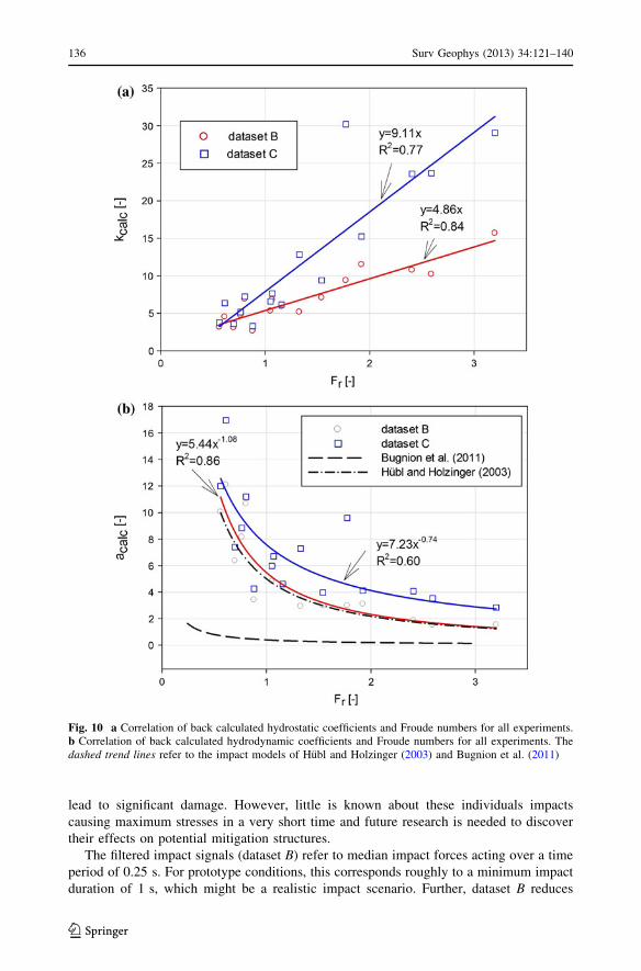
The back calculated coefficients of the dynamic approach, based on dataset B also fit to

the range of proposed data in literature. Higher peak pressure values of dataset C also yield

a higher related dynamic coefficient. Back calculated dimensionless coefficients for all

experiments and datasets are listed in Table 5. Figure 10a shows the correlations of back

calculated hydrostatic coefficients with Froude numbers for all experiments, separated for

the datasets B and C.

The correlations of back calculated hydrodynamic coefficients with Froude numbers are

given in Figure 10b. Also shown are the correlations of the modified impact model (Eq. 3)

of Hubl and Holzinger (2003) as well as the field based dynamic impact model as proposed

Table 4 Maximum peak prototype pressure values of all experiments and the datasets B and C

Nr. Bulk mixture pBpeak* [kN/m2] pC

peak* [kN/m2] Dt [s]

1 Viscous 324.64 339.33 5.53

2 Viscous 166.76 207.16 5.62

3 Viscous 320.19 359.97 4.89

4 Viscous 194.32 258.51 0.58

5 Granular 284.57 398.82 0.56

6 Granular 289.36 313.94 0.67

7 Granular 392.40 411.98 0.60

8 Granular 145.77 181.23 0.80

9 Granular 133.80 155.74 1.01

10 Granular 161.73 192.95 0.91

11 Granular 253.46 629.43 0.38

12 Granular 280.20 650.56 0.31

13 Granular 369.05 684.29 0.58

14 Granular 428.47 568.06 1.27

15 Granular 337.63 740.12 0.26

16 Granular 386.28 1244.01 0.29

Mean value 279.29 458.51 1.52

Standard deviation 94.93 284.98 1.93

The approximate time difference between the moment when the debris-flow front reached the force plateand the moment when the maximum pressure values are observed is defined by Dt

134 Surv Geophys (2013) 34:121–140

123

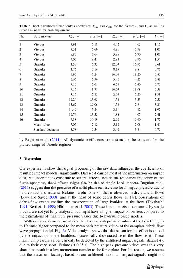
by Bugnion et al. (2011). All dynamic coefficients are assumed to be constant for the

plotted range of Froude regimes.

5 Discussion

Our experiments show that signal processing of the raw data influences the coefficients of

resulting impact models, significantly. Dataset A carried most of the information on impact

data, but uncertainties exist due to several effects. Beside the resonance frequency of the

flume apparatus, these effects might also be due to single hard impacts. Bugnion et al.

(2011) suggest that the presence of a solid phase can increase local impact pressure due to

hard contact and material locking—a phenomenon that is observed in dry granular flows

(Levy and Sayed 2008) and at the head of some debris flows. In fact, observations of

debris-flow events confirm the transportation of large boulders at the front (Takahashi

1991; Berti et al. 1999; Hurlimann et al. 2003). These hard contacts, often caused by single

blocks, are not yet fully analysed, but might have a higher impact on barriers compared to

the estimations of maximum pressure values due to hydraulic based models.

With every experiment, we also could observe peak pressure values at the flow front, up

to 10 times higher compared to the mean peak pressure values of the complete debris-flow

wave propagation (cf. Fig. 6). Video analysis shows that the reason for this effect is caused

by the impact of single boulders, occasionally dissociated from the flow front. These

maximum pressure values can only be detected by the unfiltered impact signals (dataset A),

due to their very short lifetime (&0.05 s). The high peak pressure values over this very

short time result in a low momentum transfer to the force plate. For this reason, we assume

that the maximum loading, based on our unfiltered maximum impact signals, might not

Table 5 Back calculated dimensionless coefficients kcalc and acalc, for the dataset B and C, as well asFroude numbers for each experiment

Nr. Bulk mixture kcalcB [-] kcalc

C [-] acalcB [-] acalc

C [-] Fr [-]

1 Viscous 5.91 6.18 4.42 4.62 1.16

2 Viscous 5.31 6.60 4.81 5.98 1.05

3 Viscous 6.80 7.64 5.96 6.70 1.07

4 Viscous 7.07 9.41 2.98 3.96 1.54

5 Granular 4.53 6.35 12.09 16.95 0.61

6 Granular 4.76 5.16 8.15 8.84 0.76

7 Granular 6.90 7.24 10.66 11.20 0.80

8 Granular 2.65 3.30 3.42 4.25 0.88

9 Granular 3.10 3.61 6.36 7.40 0.70

10 Granular 3.17 3.78 10.05 11.98 0.56

11 Granular 5.17 12.83 2.94 7.29 1.33

12 Granular 10.20 23.68 1.52 3.53 2.59

13 Granular 15.67 29.06 1.53 2.84 3.20

14 Granular 11.49 15.24 3.11 4.12 1.92

15 Granular 10.76 23.58 1.86 4.07 2.41

16 Granular 9.38 30.19 2.98 9.60 1.77

Mean value 7.05 12.12 5.18 7.08 1.40

Standard deviation 3.58 9.34 3.40 3.84 0.79

Surv Geophys (2013) 34:121–140 135

123

lead to significant damage. However, little is known about these individuals impacts

causing maximum stresses in a very short time and future research is needed to discover

their effects on potential mitigation structures.

The filtered impact signals (dataset B) refer to median impact forces acting over a time

period of 0.25 s. For prototype conditions, this corresponds roughly to a minimum impact

duration of 1 s, which might be a realistic impact scenario. Further, dataset B reduces

Fig. 10 a Correlation of back calculated hydrostatic coefficients and Froude numbers for all experiments.b Correlation of back calculated hydrodynamic coefficients and Froude numbers for all experiments. Thedashed trend lines refer to the impact models of Hubl and Holzinger (2003) and Bugnion et al. (2011)

136 Surv Geophys (2013) 34:121–140

123

random effects and the back calculated impact coefficients are within the range of the

proposed coefficients proposed in the literature.

The entire dataset C of the lowpass filtered impact signals reduced the observed peak

pressure values of dataset A, but showed the same integral of impact signals over time as

dataset B. No outstanding peak pressure values can be detected, but still for dataset C the

minimum approximated impact duration of one single signal amounts to 0.20 s and shows

on average 50 % higher peak pressure values, compared to the results of the averaged

datasets B. However, peak pressure values of dataset C are within the range of uncertainty

of dataset B for all experiments.

Nevertheless, impact models based on a reduced dataset might miss information of peak

pressure values based on single hard impacts, acting over a longer time period. Here, more

research is needed to define a critical duration of impacts or modified design criteria based

on impact duration.

A clear distinction between viscous and granular setups can be observed, regarding the

time difference ðDtÞ between the moment when the debris-flow front reached the force

plate and the moment when the maximum pressure values were measured. Here, maximum

pressure values for the granular setups were constantly measured close to the point in time

when the debris-flow front reached the force plate. For the viscous setups, we observed a

significant time lag between the first impact and the maximum measured impact. This

retarded reaction might be due to an increase in the pore water pressure from the debris-

flow front to its tail caused by the fine material within the bulk mixture.

The Austrian code series, which is currently under development, considers the hydro-

static model proposed by Armanini (1997) and the modified hydrodynamic model of Hubl

and Holzinger (2003). In principle, our data show that the dynamic impact coefficients

linearly correlate to the inverse of the Froude numbers (Fig. 10b). The peak pressures can

therefore also be estimated by means of:

ppeak ¼ �qdf vðghÞ1=2 ð14Þ

with � reflecting the dimensionless impact coefficients (k and a) at Froude number Fr = 1.

Since we assume Froude scaling (� is constant for the applied Froude range) we sub-

stitute Eq. 14 with

ðghÞ1=2 / v ð15Þ

resulting in

ppeak ¼ �qdf v2 ð16Þ

Figure 10b as well as Eqs. (14–16) show that the modified impact model (Eq. 3), as

proposed by Hubl and Holzinger (2003), is very close to the general form of the dynamic

impact model (Eq. 2), which is physically approved and confirmed by several experiments.

However, considering the hydrodynamic model in detail ð� ¼ aÞ, our data show higher

back calculated dynamic impact coefficients with increasing Froude numbers (Table 5).

The divergence between the correlation proposed by Bugnion et al. (2011) and the cor-

relation found for this study and for Hubl and Holzinger (2003) (Fig. 10b) might be

explained by the different examined process types (hill slope debris flows vs. debris flows).

Further, data of this study as well as of Hubl and Holzinger (2003) are based on a small

scale modelling approach, whereas the real-scale experiments by Bugnion et al. (2011)

showed higher turbulences, respectively, higher turbulence and higher Froude numbers. It

Surv Geophys (2013) 34:121–140 137

123

seems that the variable impact coefficients due to the complex rheological characteristics

of the flowing mass is to some extent reflected by the Froude regime. These aspects need to

be further evaluated with laboratory and field data.

6 Conclusion

The small scale modelling approach to measure horizontal debris-flow forces is confirmed

by existing impact models, although our study shows that the kind of signal processing of

the raw impact data has a big influence. The correlation between the Froude numbers and

the dimensionless coefficients of the hydrostatic and hydrodynamic models underline the

approach to fulfil kinematic similarity when analysing debris-flow impact forces based on a

physical model in the laboratory. We further conclude that the general form of the

dynamical impact model shows more plausible results, compared to the general form of the

hydrostatic model.

Typically, load cases for dimensioning debris-flow barriers account either for a single

block impact or for hydrostatic or hydrodynamic impacts, which act over the total flow

height. Our small scale experiments gave evidence to debate a combination or enlargement

of these two load cases, considering individual punctual impacts, causing maximum

stresses at the moment when the flow front hits the structure.

Acknowledgments The study is part of the research project ‘‘Historical arch bridges under horizontaldebris flow impacts’’ funded by the Austrian Science Fund (FWF), project nr.: P21653. The authors thankProf. Dr. Ottner from the Institute of Applied Geology (BOKU) for analysing the clay material, and Dr. Sinnfrom the Institute of Physics and Material Sciences (BOKU) for providing us the technology to calibrate theload cells used in this study. The authors also thank Fabian Steinkellner for his fundamental work on thedesign of the force plate panel.

Open Access This article is distributed under the terms of the Creative Commons Attribution Licensewhich permits any use, distribution, and reproduction in any medium, provided the original author(s) and thesource are credited.

References

Arattano M, Franzi L (2003) On the evaluation of debris flows dynamics by means of mathematical models.Nat Hazards Earth Syst Sci 3(6):539–544. doi:10.5194/nhess-3-539-2003

Armanini A (1997) On the dynamic impact of debris flows. In: Armanini A, Masanori M (eds) Recentdevelopments on debris flows, lecture notes in earth sciences, Springer, Berlin, pp 208–226

Armanini A, Scotton P (1992) Experimental analysis on the dynamic impact of a debris flow on structures.In: Internationales symposion interpraevent 1992, vol 6, Bern, pp 107–116

Berti M, Genevois R, Simoni A, Tecca PR (1999) Field observations of a debris flow event in the dolomites.Geomorphology 29:265–274. doi:10.1016/S0169-555X(99)00018-5

Bugnion L, McArdell B, Bartelt P, Wendeler C (2011) Measurements of hillslope debris flow impactpressure on obstacles. Landslides, pp 1–9. doi:10.1007/s10346-011-0294-4

Cui P, Chen X, Waqng Y, Hu K, Li Y (2005) Jiangia ravine debris flows in southwestern china. In: Jakob M,Hungr O (eds) Debris-flow hazards and related phenomena, Springer, Berlin, pp 565–594

D’Agostino V, Cesca M, Marchi L (2010) Field and laboratory investigations of runout distances of debrisflows in the dolomites (eastern italian alps). Geomorphology 115(3-4):294–304. doi:10.1016/j.geomorph.2009.06.032

Davies T (1994) Dynamically similar small-scale debris flow models. In: University of Trento I (ed) Inter-national workshop on floods and inundations related to large earth movements, IAHS Publication, p 11

DeNatale J, Iverson R, Major J, LaHusen R, Fiegel G, Duffy J (1999) Experimental testing of flexiblebarriers for containment of debris flows. US Geological Survey Open-File Report 205:38

138 Surv Geophys (2013) 34:121–140

123

Egli T (2005) Wegleitung, Objektschutz gegen gravitative Naturgefahren. Vereinigung Kantonaler Feuer-versicherungen (VKF)

Hu K, Wei F, Li Y (2011) Real-time measurement and preliminary analysis of debris-flow impact force atjiangjia ravine, china. Earth Surf Process Landf 36:1268–1278 doi:10.1002/esp.2155

Hubl J, Holzinger G (2003) Entwicklung von Grundlagen zur Dimensionierung kronenoffener Bauwerke furdie Geschiebebewirtschaftung in Wildbachen: Kleinmassstabliche Modellversuche zur Wirkung vonMurbrechern. WLS Report 50 Band 3, Institut of Mountain Risk Engineering

Hubl J, Suda J, Proske D, Kaitna R, Scheidl C (2009) Debris flow impact estimation. In: Popovska C,Jovanovski M (eds) Eleventh international symposium on water management and hydraulic Engi-neering, vol 1, pp 137–148

Hurlimann M, Rickenmann D, Graph C (2003) Field and monitoring data of debris-flow events in the swissalps. Can Geotech J 40:161–175

Ishikawa N, Inoue R, Hayashi K, Hasegawa Y, Mizuyama T (2008) Experimental approach on measurementof impulsive fluid force using debris flow model. In: Conference proceedings interpraevent 08

Iverson RM (1997) The physics of debris flows. Rev Geophys 35(3):245–296Iverson RM, Denlinger RP (2001) Flow of variably fluidized granular masses across three-dimensional

terrain. J Geophys Res 106:537–552. doi:1.1029/2000JB900329Iverson RM, Reid ME, Logan M, LaHusen RG, Godt JW, Griswold JP (2011) Positive feedback and

momentum growth during debris-flow entrainment of wet bed sediment. Nat Geosci 4(2):116–121. doi:10.1038/ngeo1040

Kherkheulidze I (1969) Estimation of basic characteristics of mudflows (‘sel’). In: Floods and their com-putation, International Association of Scientific Hydrology Publication, Leningrad, vol 2, 940–948

Konig U (2006) Real scale debris flow tests in the Schesatobel-valley. Master’s thesis, University of NaturalResources and Life Sciences, Vienna, Austria

Levy A, Sayed M (2008) Numerical simulations of the flow of dilute granular materials around obstacles.Powder Technol 181(2):137–148. doi:10.1016/j.powtec.2006.12.005

Lichtenhahn C (1973) Die Berechnung von Sperren in Beton und Eisenbeton. In: Kolloquium uber Wild-bachsperren, Mitteilungen der Forstlichen Bundesanstalt Wien, vol 102, pp 91–127

Monney J, Herzog B, Wenger M, Wendeler C, Roth A (2007) Einsatz von multiplen Stahlnetzbarrieren alsMurgangruckhalt. Wasser Energie Luft 3:255–259

S, Suwa H, Okunishi K, Nakano K, K Y (1977) General observations of debris flow (iii),1976 yakedakekamikamihorizawa. In: Annual report of the Disaster Prevention Research Institute at Kyoto Uni-versity, vol 20B, pp 237–263

Proske D, Kaitna R, Suda J, Hubl J (2008) Abschatzung einer Anprallkraft fur murenexponierte Massi-vbauwerke. Bautechnik 85(12):803–811. doi:10.1002/bate.200810059

Scotton P, Deganutti A (1997) Phreatic line and dynmaic impact in laboratory debris flow experiments. In:Chen C (ed) Proceedings of the 1st. international conference on debris-flow hazards mitigation:mechanics, prediction and assessment, American Society of Civil Engineers, New York, pp 777 – 786

Shieh CL, Ting CH, Pan HW (2008) Impulsive force of debris flow on a curved dam. Int J Sediment Res23:149–158. doi:10.1016/S1001-6279(08)60014-1

Takahashi T (1991) Debris flow. IAHR Monograph Series, A.A.Balkema / Rotterdam / BrookfieldTecca PR, Galgaro A, Genevois R, Deganutti A (2003) Development of a remotely controlled debris flow

monitoring system in the dolomites (acquabona, italy). Hydrol Process 17:1771–1784Thornton C (1997) Coefficient of restitution for collinear collisions of elastic-perfectly plastic spheres.

J Appl Mech 64(2):383–386. doi:10.1115/1.2787319Tiberghien D, Laigle D, Naaim M, Thibert E, Ousset F (2007) Experimental investigation of inter-action

between mudflow and obstacle. In: Chen C, Major J (eds) Debris-flow hazards mitigation: mechanics,prediction and assessment, Millpress, Rotterdam

VanDine DF (1996) Debris flow control structures for forest engineering. Working paper, Ministry of ForestResearch Program, Victoria, British Columbia

VAW (1992) Murgange 1987, Dokumentation und Analyse, Bericht Nr.: 97.6 der Versuchsanstalt furWasserbau, Hydrologie und Glaziologie, ETH Zurich

Walton O, Braun RL (1986) Viscosity, granular-temperature, and stress calculations for shearing assembliesof inelastic frictional disks. J Rheol 30:949–980

Watanabe M, Ike (1981) Investigation and analysis of volcanic mud flows on mount sakurajima. japan. In:Erosion sediment transport measurement, International Association on Hydrology, Florence, SciencePublication, vol 133, 245–256

Wendeler C (2008) Murgangsruckhalt in wildbachen. grundlage zur planung und berechnung von flexiblenbarrieren. PhD thesis, Swiss Federal Institute of Technology Zurich, Zurich. doi:10.3929/ethz-a-005699588

Surv Geophys (2013) 34:121–140 139

123

Wendeler C, Volkwein A, Denk M, Roth A, Wartmann S (2007) Field measurements used for numericalmodelling of flexible debris flow barriers. In: Chen C, Major J (eds) Debris-flow hazards mitigationmechanics, prediction and assessment, Millpress, Rotterdam

Zhang S (1993) A comprehensive approach to the observation and prevention of debris flows in china. NatHazards 7:1–23. doi:10.1007/BF00595676

140 Surv Geophys (2013) 34:121–140

123