analysis and applications of some modified bessel …dlozier/sf21/sf21slides/rappoport4.pdf ·...
TRANSCRIPT

ANALYSIS AND APPLICATIONS OF SOME MODIFIED BESSEL FUNCTIONS
JURI M. RAPPOPORT∗
Abstract. Some new properties of kernels of modified Kontorovitch–Lebedev integral transforms — modifiedBessel functions of the second kind with complex orderK 1
2+iβ(x) are presented. Inequalities giving estimations for
these functions with argumentx and parameterβ are obtained. The polynomial approximations of these functionsas a solutions of linear differential equations with polynomial coefficients and their systems are proposed.
Key words. Chebyshev polynomials, modified Bessel functions, Lanczos Tau method, Kontorovich-Lebedevintegral transforms
AMS subject classifications.33C10, 33F05, 65D20
1. Some properties of the functionsReK 12+iβ(x) and ImK 1
2+iβ(x). In this sectionnew properties of the kernels of modified Kontorovitch–Lebedev integral transforms are de-duced, and some of their known properties are collected, which are necessary later on.
It is possible to write the kernels of these transforms in the form
ReK 12+iβ(x) =
K 12+iβ(x) +K 1
2−iβ(x)
2and ImK 1
2+iβ(x) =K 1
2+iβ(x)−K 12−iβ(x)
2i,
whereKν(x) is the modified Bessel function of the second kind (also called MacDonaldfunction).
The functionsReK 12+iβ(x) andImK 1
2+iβ(x) have integral representations [1]
(1.1) ReK 12+iβ(x) =
∫ ∞
0
e−x cosh t cosht
2cos(βt)dt,
(1.2) ImK 12+iβ(x) =
∫ ∞
0
e−x cosh t sinht
2sin(βt)dt.
The vector-function(y1(x), y2(x)) with the componentsy1(x) = ReK 12+iβ(x),
y2(x) = ImK 12+iβ(x) is the solution of the system of differential equations
d2y1dx2
+1x
dy1dx
−(
1 +14 − β2
x2
)y1 +
β
x2y2 = 0,
d2y2dx2
+1x
dy2dx
− β
x2y1 −
(1 +
14 − β2
x2
)y2 = 0.
The functionsReK 12+iβ(x) andImK 1
2+iβ(x) are even and odd functions, respectivelyof the variableβ,
ReK 12+iβ(x) = ReK 1
2−iβ(x),
ImK 12+iβ(x) = −ImK 1
2−iβ(x).
∗Russian Academy of Sciences, Vlasov Street, Building 27, Apt. 8, Moscow 117335, Russia([email protected] ).
1

2 J. M. RAPPOPORT
The functionsReK 12+iβ(x) andImK 1
2+iβ(x) are related to the modified Bessel func-tions of the first kindIν(x) as follows,
(1.3) ReK 12+iβ(x) =
π
cosh(πβ)
ReI− 12−iβ(x)−ReI 1
2+iβ(x)
2,
(1.4) ImK 12+iβ(x) =
π
cosh(πβ)
ImI− 12−iβ(x)− ImI 1
2+iβ(x)
2.
The expansion ofI 12+iβ(x) in ascending powers ofx has the form
I 12+iβ(x) =
(x2
) 12(cos(β ln
x
2
)+ i sin
(β ln
x
2
))×
∞∑k=0
(x2
4
)k
k!Γ(k + 3
2 + iβ) =
∞∑k=0
(ak + ibk),(1.5)
whereak andbk satisfy the following recurrence relations:
a0 + ib0 =(x
2
) 12 cos
(β ln x
2
)+ i sin
(β ln x
2
)Γ(
32 + iβ
) ,
mk = x2 k + 12
4k((k + 1
2
)2 + β2) , nk = x2 β
4k((k + 1
2
)2 + β2) ,
ak = ak−1mk + bk−1nk, bk = bk−1mk − ak−1nk.
The expansion ofI− 12−iβ(x) in ascending powers ofx has the form
I− 12−iβ(x) =
(x2
)− 12(cos(β ln
x
2
)− i sin
(β ln
x
2
))×
∞∑k=0
(x2
4
)k
k!Γ(k + 1
2 − iβ) =
∞∑k=0
(ck + idk),(1.6)
whereck anddk satisfy the following recurrence relations:
c0 + id0 =(x
2
)−1/2 cos(β ln x
2
)− i sin
(β ln x
2
)Γ(
12 − iβ
) ,
pk = x2 k − 12
4k((k − 1
2
)2 + β2) , qk = x2 β
4k((k − 1
2
)2 + β2) ,
ck = ck−1pk − dk−1qk, dk = dk−1pk + ck−1qk.
The expansions (1.5) and (1.6) converge for all0 < x <∞ and0 ≤ β <∞.It follows from (1.1)–(1.2) that it is possible to writeReK 1
2+iβ(x) in the form of theFourier cosinus-transform
(1.7) ReK 12+iβ(x) =
(π2
) 12FC
[e−x cosh t cosh
t
2; t→ β
],
MODIFIED BESSEL FUNCTIONS 3
andImK 12+iβ(x) in the form of the Fourier sinus-transform
(1.8) ImK 12+iβ(x) =
(π2
) 12FS
[e−x cosh t sinh
t
2; t→ β
].
The inversion formulas have the respective forms
FC
[ReK 1
2+iβ(x);β → t]
=(π
2
) 12e−x cosh t cosh
t
2,
FS
[ImK 1
2+iβ(x);β → t]
=(π
2
) 12e−x cosh t sinh
t
2
or, in integral form,∫ ∞
0
ReK 12+iβ(x) cos(tβ)dβ =
π
2e−x cosh t cosh
t
2,(1.9) ∫ ∞
0
ImK 12+iβ(x) sin(tβ)dβ =
π
2e−x cosh t sinh
t
2.(1.10)
Differentiating equations (1.9) and (1.10) with respect tot, we obtain∫ ∞
0
βReK 12+iβ(x) sin(tβ)dβ =
π
2
(x sinh t cosh
t
2− sinh
t
2
)e−x cosh t,∫ ∞
0
βImK 12+iβ(x) cos(tβ)dβ =
π
2
(cosh
t
2− x sinh t sinh
t
2
)e−x cosh t.(1.11)
It follows from (1.9) that ∫ ∞
0
ReK 12+iβ(x)dβ =
π
2e−x,
and from (1.11) that ∫ ∞
0
βImK 12+iβ(x)dβ =
π
2e−x.
Differentiating (1.9) and (1.10) 2n times with respect tot, we obtain∫ ∞
0
β2nReK 12+iβ(x) cos(tβ)dβ =
π
2(−1)nD2n
t
(e−x cosh t cosh
t
2
),∫ ∞
0
β2nImK 12+iβ(x) sin(tβ)dβ =
π
2(−1)nD2n
t
(e−x cosh t sinh
t
2
),
from which there follows, fort = 0,∫ ∞
0
β2nReK 12+iβ(x)dβ =
π
2(−1)nD2n
t
(e−x cosh t cosh
t
2
)t=0
.
Differentiating (1.9) and (1.10) 2n+ 1 times with respect tot, we obtain∫ ∞
0
β2n+1ReK1/2+iβ(x) sin(tβ)dβ =π
2(−1)n+1D2n+1
t
(e−x cosh t cosh
t
2
),∫ ∞
0
β2n+1ImK1/2+iβ(x) cos(tβ)dβ =π
2(−1)nD2n+1
t
(e−x cosh t sinh
t
2
).
4 J. M. RAPPOPORT
whence, fort = 0,∫ ∞
0
β2n+1ImK1/2+iβ(x)dβ =π
2(−1)nD2n+1
t
(e−x cosh t sinh
t
2
)t=0
.
For the computation of certain integrals of the functionsReK 12+iβ(x) and ImK 1
2+iβ(x),integral identities are useful. They reduce this problem to the computation of some otherintegrals of elementary functions.
PROPOSITION1.1. If f is absolutely integrable on[0,∞), then the following identitieshold, ∫ ∞
0
ReK 12+iβ(x)f(β)dβ =
(π2
) 12∫ ∞
0
e−x cosh t cosht
2FC(t)dt,(1.12) ∫ ∞
0
ImK 12+iβ(x)f(β)dβ =
(π2
) 12∫ ∞
0
e−x cosh t sinht
2FS(t)dt,(1.13)
whereFC(t) is the Fourier cosinus-transform off(β), andFS(t) the Fourier sinus-transformof f(β).
Proof. Multiplying both sides of the equalities (1.7) and (1.8) by f(β), integrating withrespect toβ from 0 to∞, and applying Fubini’s theorem for singular integrals with parameter[2], we obtain (1.12) and (1.13).
PROPOSITION1.2. If f is absolutely integrable on[0,∞), then the following identitieshold ∫ ∞
0
ReK 12+iβ(x)FC(β)dβ =
(π2
) 12∫ ∞
0
e−x cosh t cosht
2f(t)dt,(1.14) ∫ ∞
0
ImK 12+iβ(x)FS(β)dβ =
(π2
) 12∫ ∞
0
e−x cosh t sinht
2f(t)dt.(1.15)
Proof. This follows from (1.9)–(1.10) and from Fubini’s theorem [2].The equations (1.12)–(1.15) are useful for the simplification and the calculation of dif-
ferent integrals containingReK1/2+iβ(x) andImK1/2+iβ(x).
For example, letf(β) = e−αβ , thenFC(t) =√
2π
αα2+t2 , FS(t) =
√2π
tα2+t2 and∫ ∞
0
ReK 12+iβ(x)e−αβdβ = α
∫ ∞
0
(α2 + t2)−1e−x cosh t cosht
2dt,∫ ∞
0
ReK 12+iβ(x)
1α2 + β2
dβ =π
2α
∫ ∞
0
e−αt−x cosh t cosht
2dt,∫ ∞
0
ImK 12+iβ(x)e−αβdβ =
∫ ∞
0
t(α2 + t2)−1e−x cosh t sinht
2dt,∫ ∞
0
ImK 12+iβ(x)
β
α2 + β2dβ =
π
2
∫ ∞
0
e−αt−x cosh t sinht
2dt.
If f(β) = Γ( 14 + iβ
2 )Γ( 14 −
iβ2 ), thenFC(t) = 2π√
cosh tand∫ ∞
0
ReK 12+iβ(x)Γ(
14
+iβ
2)Γ(
14− iβ
2)dβ =
=√
2ππ∫ ∞
0
e−x cosh t cosh t2√
cosh tdt = π
√πe−
x2K0(
x
2).
MODIFIED BESSEL FUNCTIONS 5
If f(β) = sinh(2πβ)cosh(2πβ)+cos(2πα) , |Reα| < 1
2 , thenFS(t) = cosh(αt)√2π sinh t
2and
∫ ∞
0
ImK 12+iβ(x) sinh(2πβ)
cosh(2πβ) + cos(2πα)dβ =
12
∫ ∞
0
e−x cosh t cosh(αt)dt =12Kα(x).
REMARK 1.3. All formulas of the present paragraph remain valid ifx is changed tozlying in the right-hand half-plane.
1.1. The Laplace transform ofReK 12+iβ(x) and ImK 1
2+iβ(x).The Laplace transform ofKiβ(x) is computed in [3]. We use the representation (1.1) for theevaluation of the Laplace transformation ofReK 1
2+iβ(x). We have
L[ReK 1
2+iβ(x);β]
=∫ ∞
0
cos(βt) cosht
2
∫ ∞
0
e−(p+cosh t)x dx dt
=∫ ∞
0
cos(βt) cosh t2
cosh t+ coshαdt (p = coshα)
=√π
2FC
(cosh t
2
cosh t+ coshα
)=π
2cos(αβ)
cosh α2 cosh(πβ)
.
Equivalently, we can write
L−1
cos(β cosh−1 p)√p+12
=(π
2
)−1
cosh(πβ)ReK 12+iβ(x).
For the evaluation of the Laplace transform ofImK 12+iβ(x) we utilize the representation
(1.2). We have
L[ImK 1
2+iβ(x); p]
=√π
2FS
(sinh t
2
cosh t+ coshα
)=π
2sin(αβ)
cosh(πβ) sinh α2
,
or, equivalently,
L−1
sin(β cosh−1 p)√p−12
=√π
2cosh(πβ)ImK 1
2+iβ(x).
We note that these equations can also be obtained directly from the formula for the Laplacetransforms ofKν(x) by separating real and imaginary parts.
1.2. The asymptotic behavior ofReK 12+iβ(x) and ImK 1
2+iβ(x) for x → 0, x → ∞and β → ∞. ForReK 1
2+iβ(x) andImK 12+iβ(x) the following asymptotic formulas for
β →∞ are valid [1],
ReK 12+iβ(x) ∼
(πx
) 12e−
πβ2 cos
(β lnβ − β − β ln
x
2
),
ImK 12+iβ(x) ∼
(πx
) 12e−
πβ2 sin
(β lnβ − β − β ln
x
2
),
wherex is a fixed positive number.

6 J. M. RAPPOPORT
It follows immediately from (1.3)–(1.6) that forx→ 0 we have
K 12+iβ(x) ∼ 1
2
(x2
)− 12 cos
(β ln x
2
)− i sin
(β ln x
2
)Γ(
12 − iβ
) ,
whence
ReK 12+iβ(x) ∼ 1
2
(x2
)− 12
(ReΓ
(12
+ iβ
)cos(β ln
x
2
)+ImΓ
(12
+ iβ
)sin(β ln
x
2
)),
ImK 12+iβ(x) ∼ 1
2
(x2
)− 12
(ImΓ
(12
+ iβ
)cos(β ln
x
2
)−ReΓ
(12
+ iβ
)sin(β ln
x
2
)),
For large valuesx the following asymptotic expansion is valid [4]
K 12+iβ(x) ∼
( π2x
) 12e−x
∞∑k=0
(12
+ iβ, k
)(2x)−k,
where
(ν, k) =(4ν2 − 12)(4ν2 − 32) · · · (4ν2 − (2k − 1)2)
22kk!.
In particular, therefore,
ReK 12+iβ(x) ∼
( π2x
) 12e−x
(1− β2
2x+ · · ·
),
ImK 12+iβ(x) ∼
( π2x
) 12e−x
(β
2x+ · · ·
)=
β
2x
( π2x
) 12e−x(1 + · · · ).
1.3. The series expansions in powers ofβ. The solutions of problems in mathemat-ical physics connected with the use of the Kontorovitch–Lebedev integral transforms areoften expressed as integrals with respect toβ of the functionsKiβ(x), ReK 1
2+iβ(x) andImK 1
2+iβ(x). Both the asymptotic expansions of these integrals for large valuesβ, and theexpansions of these functions in powers ofβ, are of interest for the analysis of the behaviorof these integrals.
The expansions of these functions in powers ofβ are deduced from their integral repre-sentations (1.1)–(1.2). Substituting in themcos(βt) andsin(βt) by their series expansionsand interchanging the order of the summation and integration, we obtain
Kiβ(x) =∞∑
k=0
β2k
(2k)!
∫ ∞
0
t2ke−x cosh tdt =
= K0(x)−β2
2!
∫ ∞
0
t2e−x cosh tdt+β4
4!
∫ ∞
0
t4e−x cosh tdt+ · · · ,(1.16)

MODIFIED BESSEL FUNCTIONS 7
ReK 12+iβ(x) =
∞∑k=0
β2k
(2k)!
∫ ∞
0
t2ke−x cosh t cosht
2dt =
= K 12(x)− β2
2!
∫ ∞
0
t2e−x cosh t cosht
2dt
+β4
4!
∫ ∞
0
t4e−x cosh t cosht
2dt+ · · · ,(1.17)
ImK 12+iβ(x) =
∞∑k=0
β2k+1
(2k + 1)!
∫ ∞
0
t2k+1e−x cosh t sinht
2dt =
= β
∫ ∞
0
te−x cosh t sinht
2dt− β3
3!
∫ ∞
0
t3e−x cosh t sinht
2dt+ · · · .(1.18)
These functions are entire functions in the variableβ, and therefore the series convergefor all real values ofβ. From these expansions it is possible to obtain the series for thederivatives and for the integrals of these functions with respect to the variableβ, which willconverge for all realβ also. Similar integrals for the spherical functions are stated in [5].
It’s possible to rewrite the expansions (1.16)–(1.18) in terms of Laplace transforms asfollows,
Kiβ(x) = e−x∞∑
k=0
(−1)kL
[arccosh2k(y + 1)√
(y + 1)2 − 1; y → x
]β2k
(2k)!,(1.19)
ReK 12+iβ(x) = e−x
∞∑k=0
(−1)kL
[arccosh2k(y + 1)√
2y; y → x
]β2k
(2k)!,(1.20)
ImK 12+iβ(x) = e−x
∞∑k=0
(−1)kL
[arccosh2k+1(y + 1)√
2(y + 2); y → x
]β2k+1
(2k + 1)!,(1.21)
This form of writing may be more convenient since it is possible to use numerical methodsfor evaluating Laplace transforms.
The expansions (1.19)–(1.21) are convenient for the calculation of the kernels of Konto-rovitch-Lebedev integral transforms for small valuesβ.
2. Inequalities for the MacDonald functionsKiβ(x),ReK 12+iβ(x) and ImK 1
2+iβ(x).It follows from (1.1) that for allβ ∈ [0,∞)
|ReK 12+iβ(x)| ≤ K 1
2(x) =
( π2x
) 12e−x,
and it follows from (1.2) that for allβ ∈ [0,∞)
|ImK 12+iβ(x)| ≤
∫ ∞
0
e−x cosh t sinht
2dt =
( π2x
) 12ex[1− φ((2x)
12 )]≤ B
e−x
x,
whereB is some positive constant [6],[7].In [8], for arbitraryν = σ + iβ, σ ≥ 0, the following inequality is derived
|Iν(x)| ≤ eπ|β|
2 Iσ(x).
Taking advantage of the formula [8]
|Kν(x)| ≤(C1(x, σ) + C2(x, σ)|β|σ− 1
2
)e−
π|β|2 ,
8 J. M. RAPPOPORT
we obtain that beginning with someT, |β| > T ,
|K 12+iβ(x)| ≤ C(x)e−
π|β|2 .
But this inequality is too rough and may be insufficient for conducting various proofs. Toobtain more refined inequalities, we use [9]
(2.1) |Kiβ(x)| ≤ Ax−14 e−
π|β|2 ,
whereA is some positive constant, and the representations [1]
ReK 12+iβ(x) =
( π2x
) 12 e−x
cosh(πβ)
+β tanh(πβ)
(2π)12
∫ x
0
[e−(x−y)
√x− y
− e−(x+y)
x12
]Kiβ(y)dy(2.2)
−β tanh(πβ)(2π)
12
∫ ∞
x
e−(x+y)
x12
Kiβ(y)y
dy,
ImK 12+iβ(x) =
βex
(2π)12
∫ ∞
x
e−yKiβ(y)y(y − x)
12dy.
LEMMA 2.1. The following inequalities hold forx > 0
|ReK 12+iβ(x)| ≤ c|β|e−
π|β|2 x−
34 +
(2πx
) 12
e−xe−π|β|,
|ImK 12+iβ(x)| ≤ c0|β|e−
π|β|2 x−
34 ,
wherec0 andc are some positive constants.Proof. We estimate the second additive term in (2.2), using the inequality (2.1),
|β tanh(πβ)(2π)
12
∫ x
0
[e−(x−y)
(x− y)12− e−(x+y)
x12
]Kiβ(y)y
dy|
≤ A|β|e−π|β|
2e−x
√x
∫ x
0
ey√1− y
x
− ey
yy−
14 dy ≤ A|β|e−
π|β|2 x−
34 .(2.3)
We next estimate the third additive term,
|β tanh(πβ)√2π
∫ ∞
x
e−(x+y)
√x
Kiβ(y)y
dy| ≤ B|β|e−π|β|
2e−x
√x
∫ ∞
x
e−yy−54 dy
≤ B|β|e−π|β|
2 e−2xx−34 .(2.4)
Combining the first term and estimates (2.3) and (2.4), we obtain the required inequality.Furthermore, we obtain
|ImK 12+iβ(x)| ≤ | βe
x
√2π
∫ ∞
0
e−yKiβ(y)y√y − x
dy|
≤ c0|β|e−π|β|
2 ex
∫ infty
x
e−yy−54
√y − x
dy ≤ c0|β|e−π|β|
2 x−34 .
MODIFIED BESSEL FUNCTIONS 9
For future use, an analysis of the behavior of the modified Bessel functionKσ+iβ(x) for largevalues ofβ is necessary.
LEMMA 2.2. For 0 ≤ σ ≤ 12 , |β| ≥ β0 ≥ 1, x ≥ x0 ≥ 1, the following inequality holds,
|Kσ+iβ(x)| ≤(c1x
σ− 12 + c2x
12−σ|β|σ− 1
2
)ex−π|β|
2 ,
wherec1 > 0, c2 > 0, c1, c2, β0, x0 are some constants.Proof. We use the formula [10]
Kµ(x) =π
2 sin(πµ)(I−µ(x)− Iµ(x)), µ = σ + iβ.
1. We first estimatesin(πµ). It is possible to show that for|β| ≥ β(1)0 > 0, β(1)
0 someconstant, the following inequality is valid
(2.5) a1eπ|β| ≤ | sin(πµ)| ≤ a2e
π|β|,
wherea1 > 0, a2 > 0, a1, a2 are some constants.2. We next estimateIµ(x), µ = σ + iβ, σ ≥ 0. The following inequality is derived for
σ ≥ 0 in [8]
|Iµ(x)| ≤ I0(x)(x2 )σe
π|β|2
Γ(σ + 1).
It follows from the asymptotics ofI0(x) [10] for largex that forx ≥ x(1)0 > 0, x(1)
0 someconstant,
(2.6) |Iµ(x)| ≤ a3xσ− 1
2 ex+π |β|
2 ,
wherea3 > 0, a3 some constant.3. We finally estimateI−µ(x), µ = σ + iβ, σ ≥ 0. Proceeding analogously [8], we can
rewriteI−µ(x) in the form
I−µ(x) =(x2 )−µ
Γ(1− µ)ψ(x, µ),
where
ψ(x, µ) = 1 +∞∑
s=1
(x2 )2s
s!∏k=s
k=1(−µ+ k).
Then|k − µ| =√
(k − σ)2 + β2 ≥ k − 1 for 0 ≤ σ ≤ 12 , k = 2, 3, . . . , and√
(1− σ)2 + β2 ≥ 12 , β arbitrary. Therefore,
∏k=sk=1
√(k − σ)2 + β2 ≥ (s−1)!
2 . We obtain,after some calculations, that
ψ(x, µ) ≤ 1 + 2∞∑
s=1
(x2 )2s
s!(s− 1)!≤ 2
(1 +
x
2I1(x)
).
Using for |β| ≥ β(2)0 ≥ 1, 0 ≤ σ ≤ 1
2 , the expansion of the gamma-function from [9]
and the asymptotics [10] for I1(x) we obtain that beginning with somex(2)0 , x ≥ x
(2)0 ≥ 1,
the following estimation holds,
(2.7) |I−µ(x)| ≤ a4x12−σ|β|σ− 1
2 ex+π|β|
2 ,

10 J. M. RAPPOPORT
a4 > 0, a4 some constant.Combining the estimations (2.5)–(2.7), we obtain that for0 ≤ σ ≤ 1
2 , |β| ≥ β0 ≥ 1,
x ≥ x0 ≥ 1, β0 = max(β(1)0 , β
(2)0 ), x0 = max(x(1)
0 , x(2)0 ) the following inequality is valid,
|Kµ(x) ≤ π
2a1e−π|β||I−µ(x)− Iµ(x)| ≤ π
2a1
(a3x
σ− 12 + a4x
12−σ|β|σ− 1
2
)ex−π|β|
2 .
Denotingc1 = π2a1
a3, c2 = π2a1
a4, we obtain the statement of the lemma.The properties of the modified Kontorovitch–Lebedev integral transforms are considered
in [11]–[14].
3. Tau method approximation for modified Bessel function of imaginary order.Several approaches for the evaluation of the modified Bessel functions are elaborated in [15]–[19]. The Tau method [20] realization, with minimal residue choice for the determination ofthe polynomial approximations of the solutions of the second order differential equations withpolynomial coefficients [16] of the following form
(a0y2 + a5y)v′′(y) + (a1y + a2)v′(y) + a3v(y) = 0, v(0) = a4, y ∈ [0, 1],
is supposed. Ann-th approximation of the solution is sought in the form of then-th degreepolynomialvn(y), which is the solution of the equation
(b0y2 + b5y)v(y) =∫ y
0
(b1x+ b2y + b3)v(x)dx+ b4y + τn+2T∗n+2[(1− αn+2)y + αn+2],
where the coefficientsai, i = 0, . . . , 5, may be expressed by coefficientsbi, i = 0, . . . , 5,αn+2 = sin2 π
4(n+2) — the leftmost root of the shifted Chebyshev polynomial of then+2-thdegreeT ∗n+2(y) in the interval[0, 1], τn+2 — undefined coefficient.
The problem about determination of the polynomialPn(y) =∑n
k=0 pkyk, which is the
least deviated from zero on the interval[0, 1] among alln-th degree polynomials, satisfyingthe pair of linear correlations on the coefficientsp0 = 0,
∑ni=1 c
(n)i pi = 1 was considered.
The following theorem is proved [16]:
THEOREM 3.1. If the sequence of numbersc(n)i , i = 1, . . . , n, is alternating, then the
polynomialτnT ∗n [(1−αn)y+αn] is the polynomial least deviating from zero in the uniformmetric on[0, 1] among all polynomials of degreen, satisfying the indicated pair of linearrelations.
On the basis of this theorem it’s shown (as suggested by us) in the Tau method residue, ina number of significant cases, is a minimal in the uniform metric on[0, 1], among all possiblepolynomial residues permitting the Volterra integral equations solution.
We have the following differential equation with polynomial coefficients for the approx-imation and computing of the second kind modified Bessel functionKiβ(x):
y2v′′(y) + 2(y + 1)v′(y) + (1/4 + β2)v(y) = 0,
v(0) = 1,
and the Volterra integral equation
y2v(y) =∫ y
0
[(94
+ β2
)x−
(14
+ β2
)y − 2
]v(x)dx+ 2y.

MODIFIED BESSEL FUNCTIONS 11
We obtain the following recurrence formulas for the coefficients of canonical polynomialsQm(y) =
∑mk=0 qkmy
k in this case:
q00 =2
14 + β2
, q0k = − 2(k + 2)k2 + k + 1
4 + β2q0k−1, k = 1, . . .
The minimality of the residue suggested by us follows from the Theorem3.1 as q0m
|q0m| =(−1)m,m = 0, 1, . . .
The advantages of this modification, as compared with usual and other tau-methods, isshown.
4. Tau method approximation for modified Bessel function of complex order.Anew numerical scheme of the Tau method application is proposed for the solution of the sec-ond order linear differential equations systems, with the second order polynomial coefficientsof the following kind:
(a(j)0 y2 + a
(j)1 y)v′′j (y) +
k∑i=1
[(a(j)3i−1y − a
(j)3i )v′i(y) + a
(j)3i+1vi(y)] = 0,
vj(0) = a(j)3k+2, j = 1, . . . , k, y ∈ [0, 1],
in the unknown vector-functionv(y) = (v1(y), . . . , vk(y)). It is assumed to have only onesolution. Integrating twice and carrying an addition in the right part in the kind of the vector-polynomialPn(y), we derive for the determination of then-th approximation of the solutionv(y) = (v1(y), . . . , vk(y)) the system of Volterra integral equations with polynomial kernels
(b(j)0 y2 + b(j)1 y)vj(y) =
∫ y
0
[k∑
i=1
(b(j)3i−1x+ b(j)3i y + b
(j)3i+1)vi(x)]dx+ Pjn+2(y),
j = 1, . . . , k,
where the coefficientsb(j)i anda(j)i , i = 0, . . . , 3k + 2 andj = 1, . . . , k, are connected in
a definite way andPjn+2(y), j = 1, . . . , k, aren + 2-th degree polynomials. The differentvariables of the vector residue choice and its minimization are analyzed. The recurrenceformulas for the canonical vector-polynomials coefficients convenient for the calculations aregiven.
Consider the system of two second order differential equations(k = 2) in more detail.This case is of particular interest for differential equations with complex coefficients.
The scheme of the integral form of the Tau Method described in this paper can be used forderiving polynomial approximations of hypergeometric and confluent hypergeometric func-tions of the first kind with complex parameters.
The modified Kontorovich–Lebedev integral transforms [11] with kernels
ReK 12+iβ(x) =
K 12 +iβ
(x)+K 12−iβ
(x)
2 andImK 12+iβ(x) =
K 12 +iβ
(x)−K 12−iβ
(x)
2i , whereKs(x)is MacDonald’s function, is of great importance in solving some problems of mathematicalphysics, in particular mixed boundary value problems for the HELMHOLTZ equation in wedgeand cone domains. We find it necessary to computeReK 1
2+iβ(x) andImK 12+iβ(x) to use this transform in practice [21]. These functions also
occur in solving some classes of dual integral equations with kernels which contain MacDon-ald’s function of imaginary indexKiβ(x) [11]. Therefore, now we consider the second kindmodified Bessel functionK 1
2+iβ(x) in more detail.

12 J. M. RAPPOPORT
We have a system of two second order differential equations
y2v′′1 + 2(y + 1)v′1 + β2v1 + βv2 = 0,
y2v′′2 + 2(y + 1)v′2 − βv1 + β2v2 = 0,
v1(0) = 1, v2(0) = 0,
or the system of Volterra integral equations
y2v1(y) =∫ y
0
((2 + β2)x− (2 + β2y))v1(x)dx+ β
∫ y
0
(x− y)v2(x)dx+ 2y,
y2v2(y) = β
∫ y
0
(y − x)v1(x)dx+∫ y
0
((2 + β2)x− (2 + β2y))v2(x)dx,
K 12+iβ(x) = (
π
2x)
12 e−x(v1(
1x
) + iv2(1x
), x ≥ 1.
The following formulas for the coefficients of canonical vector-polynomials are derived [16]
q(1)1m =
(β2 +m(m+ 1))(m+ 1)(m+ 2)(β2 +m(m+ 1))2 + β2
, q(1)2m =
β(m+ 2)(m+ 1)(β2 +m(m+ 1))2 + β2
,
q(2)1m = −q(1)2m, q
(2)2m = q
(1)1m,
q(j)1i = −
2(i+ 1)((β2 + i(i+ 1))q(j)1i+1 − βq(j)2i+1)
(β2 + i(i+ 1))2 + β2,
q(j)2i = −
2(i+ 1)(βq(j)1i+1 + (β2 + i(i+ 1))q(j)2i+1)(β2 + i(i+ 1))2 + β2
,
i = m− 1, . . . , 0, j = 1, 2.
By means of computations is shown that the choice of the residue in the formPjn+2(y) =τjn+2Tn+2[(1−αn+2)y+αn+2], j = 1, 2, is optimal as compared with other known variantsin this case too.
The applications for the numerical solution of boundary value problems in wedge do-mains are given in [22],[23].
REFERENCES
[1] N. N. LEBEDEV AND I. P. SKALSKAYA , Some integral transforms related to Kontorovitch–Lebedev trans-forms, (in Russian), in The Questions of the Mathematical Physics, pp. 68–79, Nauka, Leningrad, 1976.
[2] N. V IENER, Fourier Integral and Some Its Applications, (in Russian), Fizmatgiz, Moscow, 1963.[3] I. N. SNEDDON, The Use of Integral Transforms, McGraw-Hill, New York, 1972.

MODIFIED BESSEL FUNCTIONS 13
[4] A. F. NIKIFOROV AND V. B. UVAROV, The Special Functions of the Mathematical Physics, (in Russian),Nauka, Moscow, 1975.
[5] M. I. ZHURINA AND L. N. KARMAZINA , The Tables and Formulas for the Spherical FunctionsP m− 1
2+iτ(z),
(in Russian), VC AN SSSR, Moscow, 1962.[6] A. P. PRUDNIKOV, Y. A. BRYCHKOV, AND O. I. MARICHEV, The Integrals and Series, (in Russian), Nauka,
Moscow, 1981.[7] A. P. PRUDNIKOV, Y. A. BRYCHKOV, AND O. I. MARICHEV, The Integrals and Series, Special Functions,
(in Russian), Nauka, Moscow, 1983.[8] A. G. GRINBERG, The Selected Questions of the Mathematical Theory of the Electric and Magnetic Phe-
nomenons, (in Russian), Publishing House of AN SSSR, Moscow-Leningrad, 1948.[9] N. N. LEBEDEV, Some Integral Transforms of the Mathematical Physics, PhD Thesis, (in Russian), Ioffe
Physics-Technical Institute, Leningrad, 1950.[10] N. N. LEBEDEV, The Special Functions and Their Applications, 2nd edition, revised and complemented, (in
Russian), Fizmatgiz, Moscow-Leningrad, 1963.[11] N. N. LEBEDEV AND I. P. SKALSKAYA , The dual integral equations connected with the Kontorovitch–
Lebedev transform, (in Russian), Prikl. Matem. and Mechan., 38 (1974), pp. 1090–1097.[12] V. B. PORUCHIKOV AND J.M. RAPPOPORT, Inversion formulas for modified Kontorovitch–Lebedev trans-
forms, (in Russian), Diff. Uravn., 20 (1984), pp. 542–546.[13] J. M. RAPPOPORT, Some properties of modified Kontorovitch-Lebedev integral transforms, (in Russian), Diff.
Uravn., 21 (1985), pp. 724–727.[14] J. M. RAPPOPORT, Some results for modified Kontorovitch-Lebedev integral transforms, in Proceedings of
the 7th International Colloquium on Finite or Infinite Dimensional Complex Analysis, Marcel Dekker,2000, pp. 473–477.
[15] U. T. EHRENMARK, The numerical inversion of two classes of Kontorovich-Lebedev transforms by directquadrature, J. Comput. Appl. Math., 61 (1995), pp. 43–72.
[16] J. M. RAPPOPORT, The canonical vector-polynomials at computation of the Bessel functions of the complexorder, Comput. Math. Appl., 41 (2001), pp. 399–406.
[17] A. GIL , J. SEGURA AND N. M. TEMME, Evaluation of the modified Bessel function of the third kind ofimaginary orders, J. Comput. Phys., 175 (2002), pp. 398–411.
[18] J. M. RAPPOPORT, Some numerical quadrature algorithms for the computation of the MacDonald function,in Proceedings of the Third ISAAC Congress, Progress in Analysis, vol. 2, World Scientific Publishing,2003, pp. 1223–1230.
[19] B. R. FABIJONAS, D. L. LOZIER, AND J. M. RAPPOPORT, Algorithms and codes for the MacDonald func-tion: Recent progress and comparisons, Journ. Comput. Appl. Math., 161 (2003), pp. 179–192.
[20] J. H. FREILICH AND E. L. ORTIZ, Numerical solution of systems of ordinary differential equations with theTau Method, Math. Comp., 39 (1982), pp. 467–479.
[21] J. M. RAPPOPORT, Tables of modified Bessel functionsK 12+iβ(x), (in Russian), Nauka, Moscow, 1979.
[22] J. M. RAPPOPORT, Tau method and numerical solution of some mixed boundary value problems, in Pro-ceedings of the Conference on Computational and Mathematical Methods on Science and EngineeringCMMSE-2004, Angstrom Laboratory, 2004, pp. 236–242.
[23] J. M. RAPPOPORT, Dual integral equations for some mixed boundary value problems, in Advances in Anal-ysis, Proceedings of the 4th ISAAC Congress, World Scientific Publishing, 2005, pp. 167–176,
Tau method and numerical solution of
some mixed boundary value problems
Juri M. Rappoport
Department of Mathematical Sciences, Russian Academy of Sciences
email: [email protected]
Abstract
The new realization of the Lanczos Tau Method with minimal residue isproposed for the numerical solution of the second order differential equa-tions with polynomial coefficients. The computational scheme of Taumethod [1] is extended for the systems of hypergeometric type differen-tial equations. The programs of evaluation are prepared and tables ofthe modified Bessel functions K1/2+iβ(x) are published. A Tau Methodcomputational scheme is applied to the approximate solution of a systemof differential equations related to the differential equation of hypergeo-metric type. Various vector perturbations are discussed. Our choice ofthe perturbation term is a shifted Chebyshev polynomial with a specialform of selected transition and normalization. The minimality condi-tions for the perturbation term are found for one equation. They aresufficiently simple for the verification in number of important cases.The new applications of modified integral Kontorovitch–Lebedevtransforms [2] for the solution of some problems of mathematical physicsare given. The algorithm of numerical solution of some mixed boundaryvalue problems for the Helmholtz equation in wedge domains is devel-oped.
Key words: Lanczos Tau method, Bessel functions, Kontorovitch–Lebedev integral transforms, Chebyshev polynomials, dual integralequationMSC 2000: 65D20, 33F05, 33C10, 41A10, 65L10, 65R10
1 Tau method
The questions of the approximation of the solutions of the linear differentialequations with polynomial coefficients by means of polynomials coefficientsand construction approximations of the Kontorovitch–Lebedev integraltransforms kernels are considered. The Tau method realization with minimalresidue choice for the determination of the polynomial approximations of the
2 Tau method and numerical solution
solutions of the second order differential equations with polynomial coefficients[3] of the following form
(a0y2 + a5y)v′′(y) + (a1y + a2)v′(y) + a3v(y) = 0, v(0) = a4, y ∈ [0, 1],
is supposed. By its using n-th approximation of the solution is seeked in theform of the n-th degree polynomial vn(y), which is the solution of the equation
(b0y2+b5y)v(y) =∫ y
0(b1x+b2y+b3)v(x)dx+b4y+τn+2T
∗n+2[(1−αn+2)y+αn+2],
where coefficients ai, i=0,...,5, may be expressed by coefficients bi, i=0,...,5,αn+2 = sin2(π/(4(n + 2)))- the most left root of the shifted Chebyshev poly-nomial of the n + 2 -th degree T ∗n+2(y) in the interval [0, 1], τn+2 - undefinedcoefficient.
The problem about determination of the polynomial Pn(y) =∑n
k=0 pkyk,
which is the least deviated from zero on the interval [0, 1] among all n-thdegree polynomials, satisfying the pair of linear correlations on the coefficientsp0 = 0,
∑ni=1 c
(n)i pi = 1 was considered. The following theorem is proved:
Theorem 1. If the sequence of numbers c(n)i , i = 1, . . . , n, is alternating
then the polynomial τnT ∗n [(1 − αn)y + αn] is the polynomial least deviatingfrom zero in the uniform metric on [0, 1] among all polynomials of degree n,satisfying the indicated pair of linear relations.
On the basis of this theorem it’s shown that suggested by us in the Taumethod residue, in the number of significant cases, is the minimal in theuniform metric on [0, 1] among all possible polynomial residues permitting theVolterra integral equations solution in the kind of polynomial also.
On the example of computing the second kind modified Bessel functionKiβ(x) this modification’s advantages are shown as compared with usual andother tau-method and approximation method’s variants.
The new numerical scheme of the Tau method application is proposed forthe solution of the second order linear differential equations systems with thesecond order polynomial coefficients of the following kind:
(a(j)0 y2 + a
(j)1 y)v′′j (y) +
k∑i=1
[(a(j)3i−1y − a
(j)3i )v′i(y) + a
(j)3i+1vi(y)] = 0,
vj(0) = a(j)3k+2, j = 1, . . . , k, y ∈ [0, 1],

Juri M. Rappoport 3
in the unknown vector-function v(y) = (v1(y), . . ., vk(y)). It is assumed to haveonly one solution. Integrating twice and carrying an addition in the right partin the kind of the vector-polynomial Pn(y), we derive for the determination ofthe n-th approximation of the solution v(y) = (v1(y), . . ., vk(y)) the system ofVolterra integral equations with polynomial kernels
(b(j)0 y2 + b(j)1 y)vj(y) =
∫ y
0[
k∑i=1
(b(j)3i−1x+ b(j)3i y + b
(j)3i+1)vi(x)]dx+ Pjn+2(y),
j = 1, . . . , k,
where coefficients b(j)i and a(j)i , i = 0, . . . , 3k+2 and j = 1, . . . , k, are connected
in definite way and Pjn+2(y), j = 1, . . . , k, – n+2-th degree polynomials. Thedifferent variables of the vector residue choice and its minimization are ana-lyzed. The recurrent formulas for the canonical vector-polynomials coefficientsconvenient for the calculations are given.
Consider the system of two second order differential equations (k = 2) inmore detail. This case is of particular interest for differential equations withcomplex coefficients.
The scheme of the integral form of the Tau Method described in this papercan be used for deriving polynomial approximations of hypergeometric andconfluent hypergeometric functions of the first kind with complex parameters.
The modified Kontorovitch - Lebedev integral transforms [2] withkernels ReK1/2+iβ(x) = (K1/2+iβ(x) + K1/2−iβ(x))/2 and ImK1/2+iβ(x) =(K1/2+iβ(x) − K1/2−iβ(x))/2i, where Ks(x) is MacDonald’s function, isof great importance in solving some problems of mathematical physics, inparticular mixed boundary value problems for the Helmholtz equation inwedge and cone domains. We find it necessary to compute ReK1/2+iβ(x) andImK1/2+iβ(x) to use this transform in practice. These functions also occur insolving some classes of dual integral equations with kernels which contain Mac-Donald’s function of imaginary index Kiβ(x) [4]. Therefore, now we considerthe second kind modified Bessel function K1/2+iβ(x) in more detail.
We have a system of two second order differential equations
y2v′′1 + 2(y + 1)v′1 + β2v1 + βv2 = 0,
y2v′′2 + 2(y + 1)v′2 − βv1 + β2v2 = 0,
v1(0) = 1, v2(0) = 0,
or the system of Volterra integral equations
y2v1(y) =∫ y
0((2 + β2)x− (2 + β2y))v1(x)dx+ β
∫ y
0(x− y)v2(x)dx+ 2y,
4 Tau method and numerical solution
y2v2(y) = β
∫ y
0(y − x)v1(x)dx+
∫ y
0((2 + β2)x− (2 + β2y))v2(x)dx,
K1/2+iβ(x) = (π/(2x))1/2e−x(v1(1/x) + iv2(1/x)), x ≥ 1.
By means of computations is shown that the choice of the residue inthe form Pjn+2(y) = τjn+2Tn+2[(1 − αn+2)y + αn+2], j = 1, 2, is optimal ascompared with other known variants in this case too.
2 Mixed boundary value problems
The definition of two pairs of direct and inverse modified Kontorovitch–Lebedev integral transforms [2] are cited
F+(τ) =∫ ∞
0f(x)ReK1/2+iτ (x)dx, 0 ≤ τ ≤ ∞,
f(x) = (4/π2)∫ ∞
0ch(πτ)F+(τ)ReK1/2+iτ (x)dτ, 0 < x <∞,
andF−(τ) =
∫ ∞
0f(x)ImK1/2+iτ (x)dx, 0 ≤ τ ≤ ∞,
f(x) = (4/π2)∫ ∞
0ch(πτ)F−(τ)ImK1/2+iτ (x)dτ, 0 < x <∞.
The sufficient conditions of the existence of these transforms and the va-lidity of the inversion formulas are given.
It’s shown that the inversion formulas of the modified Kontorovitch–Lebedev integral transforms can be deduced from the inversion formulas ofthe ”usual” Kontorovitch–Lebedev transforms and the corresponding the-orem is proven.
For the case of nonnegative finite functions with restricted variation theconditions of present theorem are reduced to one condition, which is necessaryand sufficient then.
The verification of the solution of singular integral equations of the form
φ(x) = f(x) + λ
∫ ∞
0(K1(x+ y)+−K0(x+ y))φ(y)dy, 0 < x <∞,
where f(x) - given function, λ - parameter, complying with the condition λ <1/π, is given by means of the modified Kontorovitch–Lebedev transforms.The proof of the Parseval equalities for these transforms is conducted.
The problem of the evaluation of the modified Kontorovitch–Lebedevtransforms is greatly simplified by means of their decomposition into the form

Juri M. Rappoport 5
of compositions of more simple integral transforms, in particular Fourierand Laplace transforms. The expression of the modified Kontorovitch–Lebedev integral transforms over the general Meyer integral transforms ofspecial index and argument is given.
The dual integral equations with Macdonald’s function of the imaginaryorder Kiτ (x) in the kernel of the following form were introduced by Lebedevand Skalskaya [2]∫ ∞
0M(τ)τ tanh(ατ)Kiτ (kr)dτ = rg(r), 0 < r < a,
∫ ∞
0M(τ)Kiτ (kr)dτ = f(r), r > a,
where g(r) and f(r) - given functions. They showed [2] that solutions of thisequations may be determined in the form of single quadratures from solutionsof second kind Fredholm integral equations with symmetric kernel containingMacDonald’s function of the complex order K1/2+iτ (x).
M(τ) =2sqrt(2) sinh(πτ)πsqrt(π) sinh(ατ)
∫ ∞
0ψ(t)ReK1/2+iτ (kt)dt,
ψ(t) = h(t)−∫ ∞
0K(s, t)ψ(s)ds, a ≤ t <∞,
where ReK1/2+iτ (z) - real part of MacDonald’s function of complex order1/2 + iτ . In the case g(r) = 0
h(t) = −sqrt(k) exp(kt)π
d
dt
∫ ∞
0
exp(−kr)f(r)sqrt(r − t)
dr
K(s, t) =4π
∫ ∞
0
sinh[(π − α)τ ]sinh(ατ)
ReK1/2+iτ (ks)ReK1/2+iτ (kt)dτ.
The numerical solution is conducted. The economical methods of theevaluation of kernels of the integral equations based on Gauss quadratureformulas on Lagerre polynomial’s knots are proposed. The procedures ofthe preliminary transformation of integrals and extraction of the singularityin the integrand are used for the increase of accuracy and speed of algorithms.The cases of dual integral equations admitting complete analytical solution areconsidered. Observed examples demonstrate the efficiency of this approach inthe numerical solution of the mixed boundary value problems of elasticity andcombustion in the wedge domains.
The application of the integral Kontorovitch–Lebedev transforms anddual integral equations to the solution of the mixed boundary value problems
6 Tau method and numerical solution
are considered. The diffusion and elastic problems reduced to the solution ofthe proper mixed boundary value problem for the Helmholtz equation
∆u− k2u = 0,∂u
∂η|ϕ=±α,0<r<a(r) = g(r), u|ϕ=±α,r>a(r) = f(r),
u|r⇒0— restricted, u|r⇒∞— restricted.
The solution of the problem as derived by Lebedev is determined by thenext way in the form of the integral Kontorovitch–Lebedev transform
u(r, ϕ) =∫ ∞
0M(τ)
coshϕτcoshατ
Kiτ (kr)dτ,
where M(τ) is the solution of dual integral equation.It is shown that the above-mentioned problems solution for the Helm-
holtz equation are present in the form of single quadrature from Helmholtzequation are present in the form of single quadrature from Fredholm inte-gral equation type. The dimension of the problem is lowered on unit by this,what is the essential advantage of this method. The examples permitting thecomplete analitical solution of the problem are given.
The numerical solution of the mixed boundary value problems and re-ceived dual integral equations is carried out. It consists of numerical solutionof the second kind Fredholm integral equation with symmetric kernels andthe followed taking of quadratures from their solution. The estimation of erroris given. The control calculations results give the precision for the solution in6-7 digits after comma. The considered examples demonstrate the efficiency ofthe dual integral method in the solution of the mixed boundary value problemsfor the Helmholtz equation in the wedge domains.
References
[1] J.H. Freilich, E. L. Ortiz, ”Numerical solution of systems of ordinarydifferential equations with the Tau Method”, Math. Comp. 39 (1982)467–479.
[2] N.N. Lebedev, I. P. Skalskaya, ”The dual integral equationsconnected with Kontorovitch-Lebedev transform”, Prikl. Matem. andMechan. 38, no.6 (1974) 1090–1097. (in Russian).
[3] J.M. Rappoport, ”Canonical vector polynomials for the computationof complex order Bessel functions with the Tau method”, Comp. Math.Appl. 41 (2001) 399–406.

Juri M. Rappoport 7
[4] B.R. Fabijonas, D.W. Lozier, J.M. Rappoport, ”Algorithms andcodes for the Macdonald function: Recent progress and comparisons”,Journ. Comput. Appl. Math. 161 (2003) 179–192.
DUAL INTEGRAL EQUATIONS METHODFOR SOME MIXED BOUNDARY VALUEPROBLEMS
Juri M. RappoportRussian Academy of SciencesVlasov street, Building 27, Apt.8,Moscow 117335 Russian Federation ∗
Abstract The new applications of modified Kontorovitch–Lebedev integraltransforms for the solution of some problems of mathematical physicsare given. The algorithm of numerical solution of some mixed boundaryvalue problems for the Helmholtz equation in wedge domains by meansof dual integral equations method is developed.
Keywords: Dual integral equations, boundary value problems, Kontorovitch–Lebedev integral transform, modified Bessel function
1. IntroductionThe method of dual integral equations [1,4,10] is one of the effective
approaches for the solution of boundary value problems of the mathe-matical physics. The dual integral equations may be reduced to Fred-holm integral equations or infinite systems of linear algebraic equations.The special emphasis is done in this paper on dual integral equationswith modified Bessel function of imaginary index Kiτ (x) in the kernel.The problems of computation of this function are considered in [2,3,7].But the theory and applications of this type of dual integral equationsare elaborated quite unsufficiently till this time. The paper presentsimportant results for the numerical solution of these types of problems.
∗Partial funding provided by CRDF grant RM1-361.
1

2
2. The Application of Dual Integral EquationsMethod for Some Mixed Boundary ValueProblems
The modified Kontorovitch–Lebedev integral transforms [5,8] withkernels ReK1/2+iβ(x) = (K1/2+iβ(x)+K1/2−iβ(x))/2 and ImK1/2+iβ(x)= (K1/2+iβ(x) − K1/2−iβ(x))/2i, where Ks(x) is MacDonald’s func-tion, are of great importance in solving some problems of mathematicalphysics, in particular mixed boundary value problems for the Helmholtzequation in wedge and cone domains. It’s necessary to computeReK1/2+iβ(x) and ImK1/2+iβ(x) [6,7,9] to use this transforms in prac-tice. These functions also occur in solving some classes of dual inte-gral equations with kernels which contain MacDonald’s function ofimaginary index Kiβ(x). Therefore the computation of the second kindmodified Bessel function K1/2+iβ(x) is considered in more detail [6,7,9].
The definition of two pairs of direct and inverse modified Kon-torovitch–Lebedev integral transforms [5] are cited
F+(τ) =∫ ∞
0f(x)ReK1/2+iτ (x)dx, 0 ≤ τ ≤ ∞,
f(x) = (4/π2)∫ ∞
0ch(πτ)F+(τ)ReK1/2+iτ (x)dτ, 0 < x <∞,
andF−(τ) =
∫ ∞
0f(x)ImK1/2+iτ (x)dx, 0 ≤ τ ≤ ∞,
f(x) = (4/π2)∫ ∞
0ch(πτ)F−(τ)ImK1/2+iτ (x)dτ, 0 < x <∞.
The sufficient conditions of the existence of these transforms andthe validity of the inversion formulas are given.
It’s shown that the inversion formulas of the modified Kontoro-vitch–Lebedev integral transforms can be deduced from the inversionformulas of the ”usual” Kontorovitch–Lebedev transforms and thecorresponding theorem is proven. For the case of nonnegative finitefunctions with restricted variation the conditions of present theorem arereduced to one condition, which is necessary and sufficient then.
The verification of the solution of singular integral equations ofthe form
φ(x) = f(x) + λ
∫ ∞
0(K1(x+ y)+−K0(x+ y))φ(y)dy, 0 < x <∞,
where f(x) - given function, λ - parameter, complying with the conditionλ < 1/π, is given by means of the modified Kontorovitch–Lebedev

Dual Integral Equations 3
transforms. The proof of the Parseval equalities for these transformsis conducted.
The problem of the evaluation of the modified Kontorovitch–Lebedev transforms is greatly simplified by means of their decomposi-tion into the form of compositions of more simple integral transforms,in particular Fourier and Laplace transforms. The expression of themodified Kontorovitch–Lebedev integral transforms over the gen-eral Meyer integral transforms of special index and argument is given.
The dual integral equations with Macdonald’s function of theimaginary order Kiτ (x) in the kernel of the following form were intro-duced by Lebedev and Skalskaya [4]∫ ∞
0M(τ)τ tanh(ατ)Kiτ (kr)dτ = rg(r), 0 < r < a,
∫ ∞
0M(τ)Kiτ (kr)dτ = f(r), r > a,
where g(r) and f(r) - given functions. They showed [4] that solutionsof these equations may be determined in the form of single quadraturesfrom solutions of second kind Fredholm integral equations with sym-metric kernel containing MacDonald’s function of the complex orderK1/2+iτ (x)
M(τ) =2√
2 sinh(πτ)π√π sinh(ατ)
∫ ∞
0ψ(t)ReK1/2+iτ (kt)dt,
ψ(t) = h(t)−∫ ∞
0K(s, t)ψ(s)ds, a ≤ t <∞,
where ReK1/2+iτ (z) - real part of MacDonald’s function of complexorder 1/2 + iτ . In the case g(r) = 0
h(t) = −√kekt
π
d
dt
∫ ∞
0
e−krf(r)√r − t
dr,
K(s, t) =4π
∫ ∞
0
sinh[(π − α)τ ]sinh(ατ)
ReK1/2+iτ (ks)ReK1/2+iτ (kt)dτ.
The numerical solution is conducted. The economical methodsof the evaluation of kernels of the integral equations based on Gaussquadrature formulas on Laguerre polynomial’s knots are proposed.The procedures of the preliminary transformation of integrals and ex-traction of the singularity in the integrand are used for the increase ofaccuracy and speed of algorithms. The cases of dual integral equations
4
admitting complete analytical solution are considered. Observed exam-ples demonstrate the efficiency of this approach in the numerical solutionof the mixed boundary value problems of elasticity and combustion inthe wedge domains [1].
The application of the Kontorovitch–Lebedev integral trans-forms and dual integral equations to the solution of the mixed boundaryvalue problems are considered. The diffusion and elastic problems re-duced to the solution of the proper mixed boundary value problems forthe Helmholtz equation.
The mixed boundary value problems for the Helmholtz equation[4]
∆u− k2u = 0 (1)
are arised in some fields of mathematical physics.The solution of this type of problems in the wedge domains is de-
termined by the next way in the form of the Kontorovitch–Lebedevintegral transform [4]
u(r, ϕ) =∫ ∞
0M(τ)
coshϕτcoshατ
Kiτ (kr)dτ,
where M(τ) is the solution of dual integral equation.It is shown that the above-mentioned problems solution for the
Helmholtz equation are present in the form of single quadrature fromthe solution of Fredholm integral equation type. The dimension of theproblem is lowered on unit by this, what is the essential advantage ofthis method. The examples permitting the complete analitical solutionof the problem are given.
The numerical solution of the mixed boundary value problems andreceived dual integral equations is carried out. It consists of numericalsolution of the second kind Fredholm integral equation with symmet-ric kernels and the followed taking of quadratures from their solution.The estimation of error is given. The control calculations results givethe precision for the solution in 6-7 digits after comma. The consid-ered examples demonstrate the efficiency of the dual integral method inthe solution of the mixed boundary value problems for the Helmholtzequation in the wedge domains.
Let’s use the following notations here and further: r, ϕ - polarcoordinates of the point; α - angle of the sectorial domain; u - desiredfunction; η - normal to the boundary.
The numerical solution of some boundary value problems for theequation of the form (1) in arbitrary sectorial domains is considered inour work under the assumption that the function u|Γ is known on thepart of the boundary and the normal derivative ∂u
∂η |Γ is known on the

Dual Integral Equations 5
other part of the boundary. The Kontorovitch–Lebedev integraltransforms [4] and dual integral equations method [4,10] are used for thesearching of the solution.
Let’s consider the symmetric case for the simplicity of the calcu-lations
∆u− k2u = 0,∂u
∂η|ϕ=±α(r) = g(r), 0 < r < a,
u|ϕ=±α(r) = f(r), r > a,u|r→0 - restricted,u|r→∞ - restricted.
(2)
The solution of (2) is determined by the following way in the formof Kontorovitch-Lebedev integral transforms [4]
u(r, ϕ) =∫ ∞
0M(τ)
coshϕτcoshατ
Kiτ (kr)dτ, (3)
where M(τ) is the solution of dual integral equation∫∞0 M(τ)τ tanh(ατ)Kiτ (kr)dτ = rg(r), 0 < r < a,∫∞
0 M(τ)Kiτ (kr)dτ = f(r), r > a,(4)
where g(r) and f(r) - given functions and Kν(z) - modified Besselfunction (Macdonald function) of imaginary order.
The dimension of the problem is lowered on unit by this approachas it can be seen easily.
The dual integral equations of this type were considered in [4]. Itwas shown in [4] that the solutions of these equations may be determinedin the form of single quadratures from auxiliary functions satisfying tothe second kind Fredholm integral equations with symmetric kernelcontaining MacDonald’s function of the complex order K1/2+iτ (x).
The general case is reduced to the case g(r) = 0 as it follows from[4]. Let’s consider this case for the simplicity further in this paper.
Let’s denote
h(t) = −√kekt
π
d
dt
∫ ∞
0
e−krf(r)√r − t
dr,
K(s, t) =4π
∫ ∞
0
sinh[(π − α)τ ]sinh(ατ)
ReK1/2+iτ (ks)ReK1/2+iτ (kt)dτ,
(5)
where ReK1/2+iτ (z) - real part of MacDonald’s function of complexorder 1/2 + iτ .
6
Then we obtain the following procedure for the determination ofM(τ) on the basis of [4]
M(τ) =2√
2 sinh(πτ) cosh(ατ)π√π sinh(ατ)
∫ ∞
aψ(t)ReK1/2+iτ (kt)dt, (6)
where ψ(t) - solution of the integral Fredholm equation of the secondkind
ψ(t) = h(t)− k
π
∫ ∞
aK(s, t)ψ(s)ds, a ≤ t <∞. (7)
It’s useful under the decision of boundary value problems to findthe solution u on the boundary of sectorial domain
u|Γ(r) =∫ ∞
0M(τ)Kiτ (kr)dτ. (8)
Substituting expression (6) for M(τ) in (8) and transposing theorder of the integration we obtain
u|Γ(r) =2√
2π√π
∫ ∞
aψ(t)Gr(t)dt, (9)
where
Gr(t) =∫ ∞
0
sinh(πτ) cosh(ατ)sinh(ατ)
Kiτ (kr)ReK1/2+iτ (kt)dτ. (10)
So the numerical solution of the boundary value problem (2) con-sists from the numerical solution of integral Fredholm equation of thesecond kind with symmetric kernel and from the consequent taking ofthe quadratures from its solution.
Let’s truncate the integral equation (7) by the following way
ψ(t) = h(t)− k
π
∫ b
aK(s, t)ψ(s)ds, a ≤ t ≤ b. (11)
The conducted estimations show that we don’t obtain any loss ofaccuracy in the bounds 10−7−10−8 under the truncation of the integralequation (7) for b ≥ 10 in view of fast decrease of the kernels K(s, t) fors, t→∞.
The method of mechanical quadratures with the use of combinedSimpson formula with instant integration step is one of the most con-venient methods of numerical solution of Fredholm integral equationof the second kind.
The application of combined Simpson formula possible in the case
Dual Integral Equations 7
of fixed step ∆t and odd number of steps leads to the linear inhomoge-neous system of algebraic equations
ψi +∆t3k
π
N∑j=1
AjKijψj = hi, i = 1, ..., N, (12)
whereN =
b− a∆t
+ 1,
tj = a+ (j − 1)∆t, j = 1, ..., N,
Kij = K(si, tj), hi = h(ti), i, j = 1, ..., N,
ψi - approximate values ψ(ti), i = 1, ..., N,
Aj =
1 for j = 1, j = N ,4 for j = 2, 4, 6, ..., N − 1,2 for j = 3, 5, 7, ..., N − 2.
It’s convenient to use the Gauss elimination method for the solu-tion (12). The speed and operating memory of the mainframe computerBESM-6 made possible to use under the calculations up to N ≈ 150knots.
The solution of the system (12) gives values ψ1, ..., ψn. The approx-imate solution of the integral equation (7) upon the whole of interval[a, b] is found by means of interpolation over this values ψi, i = 1, ..., N.For the analytical expression of the approximate solution we take thefollowing magnitude
ψn(t) = h(t)− ∆t3k
π
n∑j=1
AjK(t, tj)ψj , (13)
having the values ψ1, ..., ψN in the points of interpolation. We obtainmore biggest accuracy in this case with respect to the comparison withlinear or quadratic interpolation.
Further the solution of dual equation was computed by the formu-las (6) with the use of codes and routines for the computationReK1/2+iτ (x) [6,7,9].
The error estimation of the numerical solution scheme (12) - (13)may be carried on.
Integrals (5), (10) may be expressed through known functions forspecial values of the angle α, in particular for α = π
n , n = 1, 2, ...We compute the truncated integrals in fact under the computa-
tions of integrals (5), (10) on the computer: the integration is carriedon over the some interval [0, B]. In view of this fact it’s important to
8
choose by the correct way the truncation interval [0, B], ensuring thecomputation of stated integrals with necesssary precision without theexpenditure of unnecessary computer time. The estimations of the error
KB(s, t) =4π
∫ ∞
B
sinh[(π − α)τ ]sinh(ατ)
ReK1/2+iτ (ks)ReK1/2+iτ (kt)dτ,
GBr (t) =
∫ ∞
B
sinh(πτ) cosh(ατ)sinh(ατ)
Kiτ (kr)ReK1/2+iτ (kt)dτ,
arising from the truncation are useful for this purpose. On the basis ofinequalities from [4,8] for functions Kiτ (x) and ReK1/2+iτ (x) we obtain
KB(s, t) ≤ c2k−3/2(st)−3/4 e−2αB
2α(B2 +
B
α+
12α2
), (14)
GBr (t) ≤ Ac
αk−1r−1/4t−3/4e−2αB, (15)
where A and c - some positive constants having the multiplicity of aunit. As it can be seen from (14) and (15) it’s necessary to take theextending interval [0, B] for the decreasing values of angle α.
Let’s consider the example admitting the complete analytical so-lution of the problem (2)
f(r) =√π
k√
2(e−kr + ekr[1− Φ(
√2k(r + a))]),
g(r) = 0, α =π
4.
Then we obtain on the basis of relevant calculations [4] that
h(t) = e−kt +1πe−kaK0(k(t+ a)),
K(s, t) = K0(k(s+ t)) +K1(k(s+ t)), (16)
and ψ(t) = e−kt.Substituting (16) in (9) and performing some calculations we ob-
tain for r < a
u|Γ(r) =√π
k√
2(e−kr(1− φ(
√2k(a− r))) + ekr(1− φ(
√2k(a+ r))))
and for r > a
u|Γ(r) =√π
k√
2(e−kr + ekr(1− φ(
√2k(a+ r))))
Dual Integral Equations 9
(verification of the conditions of the problem).We obtained the precision in 7-8 significant digits under the solu-
tion of dual integral equation (computation of the values (cosh πτ2 )−1M(τ)
) so for a = 1.0, k = 1 (cosh 3π2 )−1M(3) = .928825310 − 01.
We obtained the precision in 6-7 digits after comma under the cal-culation of values u|Γ(r) so for a = 1.0, k = 1 u|Γ(2) = .174544410 + 00.
The different preliminary procedures of the separation of singu-larity or transformation of the integral into the integral without thesingularity are useful for the computation of integral (9).
Let’s consider the calculations for the case α = π2 in detail [4].
Let’s introduce the functions
G1r(t) =π√π
2√
2e−k(r+t)√k(r + t)
and
G2r(t) =
0, t ≤ r
π√π
2√
2e−k(t−r)√k(t− r)
, t > r.
Then Gr(t) = G1r(t) +G2r(t) and
u|Γ(r) =2√
2π√π
∫ b
aψ(t)G1r(t)dt+
2√
2π√π
∫ b
max(a,r)ψ(t)G2r(t)dt. (17)
The formula (17) is more convenient for the application of procedures ofnumerical integration then formula (9).
Here the function G1r(t) hasn’t singularities for all r, t > 0 and thefunction G2r(t) hasn’t singularities for t ≥ a, r < a. For r ≥ a integrandof the second integral in (17) has singularity for t = r and the integralitself is equal to ∫ b
aψ(t)
e−k(t−r)√k(t− r)
dt.
Let’s make the change of variables t1 =√
t−rb−r and introduce the function
g(t1) =√b− rk
ψ((b− r)t21 + r)e−k(b−r)t21 .
Then the second integral in (17) is equal to 2∫ 10 g(t1)dt1, where the latter
integral doesn’t contain any singularities in the integrand.It’s strongly efficient to use the procedures of numerical integration
for the transformed integral. The accuracy of computations is increasedand the computer time is shorten by this approach.

10
3. SummaryThe dual integral equations with Macdonald’s function of the imag-
inary order Kiτ (x) in the kernel are considered. The solutions of theseequations and proper mixed boundary value problems are determinedin the form of single quadratures from solutions of second kind Fred-holm integral equations. The numerical solution is conducted and theproblems of the computational methodology are discussed. Examplesdemonstrate the efficiency of the dual integral method in the numericalsolution of the mixed boundary value problems of elasticity, combustionand electrostatics in the wedge domains.
References[1] Alexandrov, V.M., Pozharskii D.A. Nonclassical spatial problems of the mechan-
ics of contact interactions of elastic bodies. Moscow, Factorial, 1998.-288pp. (inRussian).
[2] Ehrenmark, U.T. The numerical inversion of two classes of Kontorovich–Lebedev transform of direct quadrature. Journ. Comp. Appl. Math., 61 (1995),43–72.
[3] Fabijonas, B.R., Lozier, D.W., and Rappoport J.M. Algorithms and codes forthe Macdonald function: recent progress and comparisons. Journ. Comp. Appl.Math., 161(2003), 179–192.
[4] Lebedev, N.N., and Skalskaya, I.P. Dual integral equations connected withKontorovich–Lebedev integral transform. Prikl. Matem. Mechan., 38(1974),N 6, 1090–1097 (in Russian).
[5] Lebedev, N.N., and Skalskaya, I.P. Some integral transforms relatedKontorovich–Lebedev transform. The Problems of Mathematical Physics.Leningrad: Nauka, Leningr. otd., 1976, 68–79 (in Russian).
[6] Rappoport, J.M. Tables of Modified Bessel Functions K1/2+iτ (x) . Moscow:Nauka, 1979.-338pp. (in Russian).
[7] Rappoport, J.M. The programs and some methods of the Macdonald functioncomputation. Akad. Nauk SSSR, OVM, Moscow, 1991.-16pp. (in Russian).
[8] Rappoport, J.M. Some results for modified Kontorovich–Lebedev trans-forms. Proceedings of the 7th International Colloquium on Finite or InfiniteDimensional Complex Analysis. Marcel Dekker Inc., 2000, pp.473–477.
[9] Rappoport, J.M. The canonical vector-polynomials at computation of theBessel functions of the complex order. Computers and Mathematics with Ap-plications, 2001, vol.41, No.3/4, pp.399–406.
[10] Ufliand, I.S. Method of dual equations in the mathematical physics problems.Leningrad: Nauka, Leningr. otd., 1977. - 220pp. (in Russian).
NIST Handbook of Mathematical FunctionsISBN 978-0-521-19225-5 hardbackISBN 978-0-521-14063-8 softback
NIST Digital Library of Mathematical Functions
http://dlmf.nist.gov
video
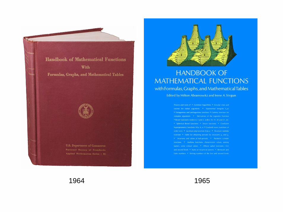
1964 1965

Milton Abramowitz Irene Stegun

Abramowitz & Stegun (1964)
0
500
1000
1500
2000
2500
1971 1978 1985 1992 1999 2006
Year
Cita
tions

From A&S to DLMF
1954 A&S project conceived1964 A&S published1996 DLMF project conceived1999 NSF grant received2008 Preliminary website released2009 CUP selected as publisher2010 DLMF published (print, cd, and web)

What’s New in DLMF?
• Methodology chapters• More formulas, fewer tables
– With references for every formula• More graphs, better graphs
– Zoomable, rotatable on web• More on computation
– With links to software on web• New functions…including Painlevé!

What Else?
• cd and web are searchable• Both have live links• Further web capabilities
– links from symbols to definitions– pop-up info boxes– online access to papers, reviews, etc.– software sections and master index– vrml and x3d visualizations
