analysis and control of batch order picking …
TRANSCRIPT

ANALYSIS AND CONTROL OF BATCH ORDER PICKING PROCESSES
CONSIDERING PICKER BLOCKING
A Dissertation
by
SOONDO HONG
Submitted to the Office of Graduate Studies of Texas A&M University
in partial fulfillment of the requirements for the degree of
DOCTOR OF PHILOSOPHY
August 2010
Major Subject: Industrial Engineering

Analysis and Control of Batch Order Picking Processes
Considering Picker Blocking
Copyright 2010 Soondo Hong

ANALYSIS AND CONTROL OF BATCH ORDER PICKING PROCESSES
CONSIDERING PICKER BLOCKING
A Dissertation
by
SOONDO HONG
Submitted to the Office of Graduate Studies of Texas A&M University
in partial fulfillment of the requirements for the degree of
DOCTOR OF PHILOSOPHY
Approved by:
Co-Chairs of Committee, Andrew A. Johnson Brett A. Peters
Committee Members, Sergiy Butenko Vivek Sarin
Head of Department, Brett A. Peters
August 2010
Major Subject: Industrial Engineering

iii
ABSTRACT
Analysis and Control of Batch Order Picking Processes Considering
Picker Blocking. (August 2010)
Soondo Hong, B.S; M.S., Pohang University of Science and Technology
Co-Chairs of Advisory Committee: Dr. Andrew A. Johnson Dr. Brett A. Peters
Order picking operations play a critical role in the order fulfillment process of
distribution centers (DCs). Picking a batch of orders is often favored when customers’
demands create a large number of small orders, since the traditional single-order picking
process results in low utilization of order pickers and significant operational costs.
Specifically, batch picking improves order picking performance by consolidating
multiple orders in a ―batch‖ to reduce the number of trips and total travel distance
required to retrieve the items. As more pickers are added to meet increased demand,
order picking performance is likely to decline due to significant picker blocking.
However, in batch picking, the process of assigning orders to particular batches allows
additional flexibility to reduce picker blocking.
This dissertation aims to identify, analyze, and control, or mitigate, picker
blocking while batch picking in picker-to-part systems. We first develop a large-scale
proximity-batching procedure that can enhance the solution quality of traditional
batching models to near-optimality as measured by travel distance. Through simulation
studies, picker blocking is quantified. The results illustrate: a) a complex relationship

iv
between picker blocking and batch formation; and b) a significant productivity loss due
to picker blocking.
Based on our analysis, we develop additional analytical and simulation models to
investigate the effects of picker blocking in batch picking and to identify the picking,
batching, and sorting strategies that reduce congestion. A new batching model (called
Indexed order Batching Model (IBM)) is proposed to consider both order proximity and
picker blocking to optimize the total order picking time. We also apply the proposed
approach to bucket brigade picking systems where hand-off delay as well as picker
blocking must be considered.
The research offers new insights about picker blocking in batch picking
operations, develops batch picking models, and provides complete control procedures
for large-scale, dynamic batch picking situations. The twin goals of added flexibility and
reduced costs are highlighted throughout the analysis.

v
ACKNOWLEDGEMENTS
I thank my dissertation advisors, Dr. Andrew L. Johnson and Dr. Brett A. Peters,
who taught me to think critically and frame the key questions. Their support encouraged
me to investigate new ideas and methods. I value their creativity and deep passion for
engineering research and their leadership in advanced education.
I am grateful to Dr. Sergiy Butenko and Dr. Vivek Sarin for their advice and
suggestions during the writing of this dissertation. I also thank Dr. Banerjee for our
constructive discussions which led me to expand my research areas.
I am fortunate to have many wonderful colleagues, including Chiwoo Park,
Youngmyoung Ko, Hyunsoo Lee, Eunshin Byon, Chaehwa Lee, and Heungjo An. I also
thank Sunghyok Woo, Byungsoo Na, Wonju Lee, Moonsu Lee, Jungjin Cho, Seongdae
Kim, Jeehyuk Park, Daeheon Choi, and Kyungnam Ha who have been good friends.
Finally, my special gratitude goes to my father, mother, brothers, mother-in-law,
father-in-law, and brother-in-law for understanding and supporting my love of research,
and I thank my wife, Misook Ha, and my son, Euipyo (Eric), for their steadfast
encouragement and love.

vi
TABLE OF CONTENTS
Page
ABSTRACT .............................................................................................................. iii
ACKNOWLEDGEMENTS ...................................................................................... v
TABLE OF CONTENTS .......................................................................................... vi
LIST OF FIGURES ................................................................................................... ix
LIST OF TABLES .................................................................................................... xii
CHAPTER
I INTRODUCTION ................................................................................ 1
II BACKGROUND .................................................................................. 5
1. Order picking systems ................................................................ 5 2. Order picking policy ................................................................... 7 3. Picker blocking ........................................................................... 9 III LITERATURE REVIEW ..................................................................... 11
1. Batch picking with k-pickers ...................................................... 11 2. Order batching algorithms .......................................................... 14 3. Research issues ........................................................................... 15
IV LARGE-SCALE ORDER BATCHING WITH TRAVERSAL ROUTING METHODS ........................................................................ 17
1. Introduction ................................................................................ 17 2. Related literature ........................................................................ 20 3. Route-selecting order batching model (RSB) ............................ 22 4. Route-bin packing problem (RPP) and its LP relaxation (RPP-
LP) ........................................................................................... 27 5. A heuristic route-packing based order batching procedure
(RBP) ......................................................................................... 31 6. Implementation and computational results ................................ 36 7. Conclusions ................................................................................ 44

vii
CHAPTER Page
V ANALYSIS OF PICKER BLOCKING IN NARROW-AISLE BATCH PICKING ............................................................................... 46
1. Introduction ................................................................................ 46 2. Literature survey ........................................................................ 50 3. Problem definition ...................................................................... 52 4. Analysis of picker blocking ........................................................ 56 5. Comparison study in parallel-aisle picking systems .................. 71 6. Conclusion and further study ..................................................... 78
VI BATCH PICKING IN NARROW-AISLE ORDER PICKING
SYSTEMS WITH CONSIDERATION FOR PICKER BLOCKING . 80 1. Introduction ................................................................................ 80 2. Literature survey ........................................................................ 82 3. Problem definition ...................................................................... 84 4. Indexed order batching model (IBM) ......................................... 87 5. An exact mixed-integer programming (MIP) formulation ......... 92 6. A simulated annealing (SA) algorithm ....................................... 105 7. Implementation and computational results ................................ 107 8. Conclusion and further studies ................................................... 117 VII ANALYSIS AND CONTROL OF PICKER BLOCKING IN A
BUCKET BRIGADE ORDER PICKING SYSTEM ........................... 119 1. Introduction ................................................................................ 119 2. Literature review ........................................................................ 124 3. Analysis and control of picker blocking .................................... 128 4. Analysis and control of hand-off delay ...................................... 137 5. Simulation and experimental results .......................................... 143 6. Conclusions ................................................................................ 155 VIII CONTRIBUTIONS AND CONCLUSION ......................................... 157
REFERENCES .......................................................................................................... 159
APPENDIX A. SUPPLEMENTARY FORMULATION, PROOF, ALGORITHM, AND RESULTS DISCUSSED IN CHAPTER IV .......................... 163
APPENDIX B. SUPPLEMENTARY EXAMPLES, PROOF, VALIDATION, ALGORITHM, AND RESULTS DISCUSSED IN CHAPTER V . 172

viii
Page
APPENDIX C. EXECUTABLE MIP FORMULATION FOR INDEXED BATCH MODEL ........................................................................................... 179
APPENDIX D. SUPPLEMENTARY FORMULATIONS AND PROOFS DISCUSSED IN CHAPTER VII ..................................................... 183
VITA ......................................................................................................................... 189

ix
LIST OF FIGURES
Page
Figure 1. Examples of order picking systems: (a) part-to-picker system (Warehouse-rx.com); (b) picker-to-part system (Amazon.com). .......................................... 5
Figure 2. A typical picker-to-part system: parallel-aisle OPS layout (Gademann et
al., 2001). .......................................................................................................... 6
Figure 3. Traversal route method (Petersen, 1997). ........................................................... 7
Figure 4. Order picking policies: (a) batch picking; (b) zone picking; and (c) bucket brigade picking. ................................................................................................ 9
Figure 5. Types of picker blocking: (a) in-the-aisle picker blocking; (b) pick-face blocking (Parikh and Meller, 2009); and (c) hand-off delay. .......................... 10
Figure 6. A ten-aisle order picking system ....................................................................... 23
Figure 7. An example of elementary route set and combined route set. .......................... 34
Figure 8. Batches b1 and b2 are constructed by grouping yr orders assigned to route r. ........................................................................................................................ 35
Figure 9. The average travel length per order with the one-way traversal routing method: (a) sort-while-pick strategy; and (b) pick-then-sort strategy. ........... 41
Figure 10. The total retrieval time comparison via a simulation study: (a) light congestion case; and (b) heavy congestion case. ............................................ 42
Figure 11. The average travel length per order with the two-way traversal routing method: (a) sort-while-pick strategy; and (b) pick-then-sort strategy. ........... 44
Figure 12. A narrow-aisle system and a routing example (modified from Gademann and Van de Velde (2005)). ............................................................................... 53
Figure 13. Picker blocking (Parikh and Meller, 2009). .................................................... 53
Figure 14. A circular order picking aisle (Gue et al., 2006). ............................................ 55
Figure 15. State space and transitions for the Markov chain model when picking time equals travel time. ................................................................................... 58

x
Page
Figure 16. The percentage of time that pickers are blocked over different number of pick faces when two pickers work with pick:walk time = 1:1........................ 60
Figure 17. The comparison of single-pick and multiple-pick models when two pickers work with pick:walk time = 1:1. ........................................................ 61
Figure 18. The percentage of time that pickers are blocked over different number of pick faces when two pickers work with pick:walk time = 1:0........................ 66
Figure 19. The comparison of single-pick and multiple-pick models when two pickers work with pick:walk time =1:0. ......................................................... 67
Figure 20. The percentage of time blocked over different pick:walk time ratios: (a) two pickers in 20 pick faces; and (b) five pickers in 100 pick faces. ............. 69
Figure 21. Simulation results over different workload distributions (the number of pickers = 5, the number of pick faces = 100, and pick:walk time = 1:0.2) : (a) the percentage of time blocked; and (b) the standard deviation of the number of picks (workload). ........................................................................... 70
Figure 22. Comparison over different batching algorithms of: (a) total travel distance; and (b) total retrieval time. .............................................................. 74
Figure 23. The percentage of time blocked and standard deviation of the number of picks per aisle over different batching algorithms: (a) FCFS; (b) seed; (c) CW II; and (d) RBP. ........................................................................................ 75
Figure 24. An example of different aisle-entrance orders due to batches skipping aisles (Bi=batch i). ........................................................................................... 90
Figure 25. Order picker’s retrieval trip starting time. ...................................................... 91
Figure 26. An OPS layout. ............................................................................................... 93
Figure 27. Delay time for batch b at pick face f when a picker is blocked. ................... 100
Figure 28. A simulated annealing algorithm. ................................................................. 106
Figure 29. A picker blocking computation procedure. ................................................... 107
Figure 30. Algorithm comparison with different throughput measurements: (a) WT+DT per order; and (b) Walk time+delay time % in the total retrieval time. .............................................................................................................. 114

xi
Page
Figure 31. A flow-rack OPS (Bartholdi and Eisenstein, 1996a). ................................... 120
Figure 32. Delay situations in bucket brigade order picking: (a) picker blocking; and (b) hand-off delay. ......................................................................................... 122
Figure 33. A description of chain reaction after completion of batch i to release a new batch i+k. ............................................................................................... 131
Figure 34. A normal situation example. In both models, four pickers process four batches. Two pickers (picker 3 and 4) may have a chance of blocking depending on items in batches i+2 and i+3 (the number of pick faces = 8, the number of pickers = 4): (a) a circular-aisle abstraction; and (b) a bucket brigade OPS. ..................................................................................... 133
Figure 35. A completion and release example. Both models release batch i+4 at the same time and it starts from pick face 1 (the number of pick faces = 8, the number of pickers = 4): (a) a circular-aisle abstraction; and (b) a bucket brigade OPS. ..................................................................................... 134
Figure 36. An example of hand-off and its appropriate renewal process. ...................... 138
Figure 37. No-handshake hand-off policy. ..................................................................... 141
Figure 38. Comparing two bucket brigade methods: (a) regular bucket brigade; and (b) no-handshake hand-off bucket brigade. .................................................. 142
Figure 39. The percentage of time blocked (two-picker, 20 pick faces) with multiple-picks with infinite backward walk with allowance of intermediate hand-off: (a) bucket brigade system; and (b) circular-aisle system. .......................................................................................................... 145
Figure 40. Impacts on hand-off delay of policy parameter over different picking environments: (a) triangular pick time; and (b) exponential pick time. ....... 148

xii
LIST OF TABLES
Page
Table 1. Computational results over different algorithms ................................................ 39
Table 2. Computational results with the two-way traversal routing method in the ten-aisle picking system .................................................................................. 43
Table 3. Default order picking and OPS profiles ........................................................... 109
Table 4. Experimental results of the exact approach ...................................................... 110
Table 5. Configuration of an OPS (modified from Petersen example (Petersen, 2000)) ............................................................................................................ 111
Table 6. Comparison of neighborhood rules in simulated annealing approach ............. 113
Table 7. Comparison of WT+DT per order .................................................................... 114
Table 8. Variation of the number of orders over two batching strategies ....................... 115
Table 9. The experimental results over diverse order picking environments ................. 116
Table 10. Comparison of inter-completion time (the number of orders=2160, Imax=20000) ................................................................................................. 117
Table 11. The percentage of time blocked when two pickers work (p=pick density, n=the number of pick faces) ......................................................................... 129
Table 12. Average hand-off delay per occurrence over different order picking situations ....................................................................................................... 146
Table 13. Summary of experimental environments ........................................................ 151
Table 14. Experimental results on single order picking ................................................. 152
Table 15. Experimental results varying batch size ......................................................... 153
Table 16. Comparison of Cont and heuristic approach (Hcont) ..................................... 154

1
CHAPTER I
INTRODUCTION
Distribution centers (DC) are a fundamental part of the supply chain, which links
manufacturers to customers. Within the supply chain, DCs consolidate and store
products, fulfill stocked products as requests arrive, and provide various value-added
functions in response to product requirements. DCs are also of economic importance;
according to the annual ―State of Logistics Report‖ (Wilson, 2008), warehousing costs in
the United States are approximately 8% of the total logistic cost, or 0.8% of total gross
domestic product (GDP).
Online retailers’ DCs are often termed ―order fulfillment facilities.‖ Their
functions include distributing customer orders and sustaining the online retail business.
Clearly, order picking operations represent significant cost and service drivers for these
retailers. According to Tompkins et al. (2003), order picking typically comprises almost
50% of the total operating costs of a typical DC. For example, in 2003, Amazon.com’s
fulfillment expense was $477 million, which accounts for 48% of total operation
expenses (Amazon.com, 2004). Amazon’s order picking operations contribute between
10-15% of its fulfillment-related expenditure, including fulfillment and customer service
centers (Lieu, 2005).
Despite the recent enhancements in order picking technology, 75 to 80%
of all DCs still rely on manual order picking (De Koster, 2004; Napolitano, 2008). ____________
This dissertation follows the style of IIE Transactions.
2
Manual order picking is cost effective because the initial setup cost is relatively low.
Moreover, human pickers are flexible relative to mechanical systems (Ruben and Jacobs,
1999) and can more easily handle irregular shapes and sizes and employ diverse sets of
picking vehicles as needed.
Since customer demands in online retailers’ order fulfillment facilities are
characterized by diverse, small-sized orders (De Koster, 2003), manual order picking
faces a critical operational issue to ensure good performance. The problem involves
determining the set of orders, i.e., the batch, to be picked by a worker, and the worker’s
route through the facility to retrieve the items in the batch. The traditional single-order
picking mode of operation can result in many costly trips, particularly if the orders are
small. In contrast, a batch order picking strategy groups orders to reduce the number of
trips required, and consequently, reduces operational costs. Additionally, the latter
strategy provides some robustness to the variation and operational difficulties caused by
small order sizes. Therefore, an efficient order batching algorithm can have a significant
impact on costs in an order picking environment with small order sizes.
In general, the number of items picked per unit of time is an important criterion
for evaluating warehouse performance (De Koster and Balk, 2008). When a shorter
fulfillment period is required, manual order picking systems tend to add more pickers to
shorten the response time. However, using a batch picking strategy with multiple pickers
introduces a new issue relevant to picker utilization, namely, that multiple pickers will
create congestion and delays that ―waste‖ productive work time. This increase in
nonproductive time is known as picker blocking. The impact of the number of pickers on

3
order picking throughput and picker utilization indicates that warehouse managers
should focus on picker blocking when assigning a large number of pickers to a particular
retrieval process. We note, however, that traditional batching algorithms do not consider
picker blocking or its impact on order picking productivity.
This dissertation is interested in order batching procedures in large-scale picking
situations with k-pickers, where picker blocking can become a significant issue. We
begin by considering a narrow-aisle picking environment, which is very attractive in
terms of storage capability. However, since one-way passage in an aisle may be
inevitable in this configuration (Gue et al., 2006), the order fulfillment time can lengthen
and the operational cost can increase, because the one-way travel characteristic leads to
longer trips and the narrow-aisle configuration produces heavy congestion Bartholdi and
Eisenstein.
Thus, we first examine the significance of picker blocking in the traditional
proximity-based batching approach. This sub-study presents a new large-scale, near-
optimal distance-based batch order picking procedure with traversal routing methods.
The operational policy identified by a gap error comparison is near-optimal based on a
travel distance criterion, but also reduces picker blocking relative to other order batching
methods. However, management is still required to reduce productivity loss due to
blocking.
Second, since the prior simulation study identifies picker blocking which is not
fully modeled by the available literature, we focus on developing an analytical model
that is suitable for batch picking and examining situations of varying levels of picker

4
activity.
Because batch picking with k-pickers appears to produce a significant level of
picker blocking when k increases to fulfill high demand levels, we propose a combined
batching and sequencing model, referred to as the indexed batching model (IBM), to
simultaneously control both the trip distance and the time blocked.
We also analyze bucket brigade picking, a popular order picking situation, where
picker blocking is still an issue but the routing issue is replaced with hand-off delay issue.
We identify analytical throughput models, build an integrated control framework to
reduce both picker blocking and hand-off delay, and derive control algorithms for each
delay case.
This dissertation is organized as follows. Chapter II describes general knowledge
and background on order picking in distribution centers. Chapter III reviews the
literature and identifies new opportunities. Chapter IV explores managing a large-size
order batching situation more efficiently and describes the effects of picker blocking.
Chapter V examines picker blocking in batch picking using analytical models and
simulation study. A new batching model that considers both proximity and congestion is
developed in Chapter VI. In Chapter VII, we discuss an application of the proposed
approach to bucket brigade systems. Chapter VIII summarizes the contributions and
highlights future research opportunities.

5
CHAPTER II
BACKGROUND
1. ORDER PICKING SYSTEMS
Order picking operation involves retrieving customer orders from storage in an
order picking system (OPS) in a DC. Commonly, a DC is composed of multiple OPSs
classified by the relevant storage and retrieval mechanism. Specifically, in part-to-picker
systems, an automated device transfers items requested to a stationary order picker
(Figure 1(a)). In picker-to-part systems, pickers travel to item storage locations and
collect the items (Figure 1 (b)). In the latter, pickers must traverse multiple aisles and
areas to fulfill orders. The travel mode can include walking with a cart or riding on a
retrieval vehicle. The skill and flexibility of the human pickers are critical, as pickers
visit multiple locations on each tour and handle diverse items.
(a) (b)
Figure 1. Examples of order picking systems: (a) part-to-picker system (Warehouse-rx.com); (b) picker-to-part system (Amazon.com).
Figure 2 shows a typical, and popular, picker-to-part picking system, i.e., a bin-
shelving picking system with a parallel-aisle configuration and two cross aisles located

6
in the front and back of the layout that connect the parallel aisles. A loading/unloading
(L/U) station is located in the front of the leftmost aisle. Bin-shelving storage on each
side of the aisles allows order pickers to easily retrieve items. One pick face includes
multiple pick locations. To collect a batch, the picker starts from the L/U station,
circumnavigates the aisles of pick area via the cross aisles, and returns to the L/U station;
this operation forms a trip.
Figure 2. A typical picker-to-part system: parallel-aisle OPS layout (Gademann et al., 2001).
A specified routing method (based on pickers’ experience or management-
determined) plays an important role in improving order picking performance, because it
determines the travel distance, which is a fundamental throughput measure. Heuristics
are often preferred because they produce more straightforward and natural routes for
pickers than an optimal strategy (Petersen and Schmenner, 1999). The heuristics include
the traversal method, the return method, the mid-point method, the largest gap method,
and the combined method (Petersen, 1997). The traversal routing method in Figure 3 is
most frequently cited in the literature because of its simplicity and popularity in industry.
When this method is used in parallel-aisle OPS, any aisle containing at least one pick is

7
traversed entirely.
Figure 3. Traversal route method (Petersen, 1997).
2. ORDER PICKING POLICY
From an operational view, organizing and batching orders for pickers to reduce
travel and blocking time is as important as designing optimal routing strategies. Single-
order picking allocates one order to one picker. Alternatively, to increase efficiency,
several orders can be consolidated in a batch. Figure 4 (a) illustrates batch picking by a
single picker. Since one picker picks multiple orders in the same trip, the total retrieval
time is reduced. When multiple orders are collected in a trip, their disassembly into
orders is termed a sorting operation. There are two efficient strategies relevant to the
sorting operation while batch picking. In the sort-while-pick strategy, pickers sort
products while traveling between picking locations. A cart carries bins for orders. The
picked items are identified as belonging to a particular order and deposited in the correct
bins. The pick-then-sort strategy separates the two operations into a sorting operation
executed by manual workers or by sortation equipment to separate the items into orders
after completing a trip to retrieve the items in a batch.
Picking a large-size batch (or order) may be assigned to multiple pickers and is

8
called zone picking (Figure 4 (b)). Order pickers travel only in their specialized zone.
There are two protocols to assign a batch to each zone. In synchronized zone picking,
each zone collects one batch simultaneously. Retrieval time for a batch can be shorter
than a full retrieval time by a single picker, because several pickers process partitioned
portions of a batch. In progressive zone picking, a batch is processed in individual zones
sequentially. A batch is passed between zones, and items are collected in various zones
to complete the orders in the batch. In general, a buffer of work-in-process batches is
formed between two zones to insure pickers in downstream zones are not idle.
Bucket brigade picking is similar to progressive zone picking, but employs a
variable zone boundary policy where zone size is not predetermined and is resized
automatically and dynamically (Figure 4 (c)). No buffer between pickers is necessary
(see, for example, Bartholdi and Eisenstein (1996a)). A batch must pass all pick faces
and collect items at related pick faces in sequence to be completed. Pickers are ordered
from upstream to downstream in a row, and the order is maintained across the zones. A
picker picks an item and places it in the tote assigned to the particular batch. The picker
then moves to the next pick face to continue processing the batch if there is no picker at
the next pick face. The upstream picker hands off the current batch when the upstream
picker meets a downstream picker who has no assigned batch.

9
(a) (b) (c)
Figure 4. Order picking policies: (a) batch picking; (b) zone picking; and (c) bucket
brigade picking.
3. PICKER BLOCKING
In a typical picker-to-part system, adding pickers is expected to enhance the
system’s order picking throughput. However, the benefits to throughput are increasingly
offset by picker blocking (Ruben and Jacobs, 1999). Picker blocking occurs when
multiple pickers traverse a pick area while maintaining a no passing restriction, or two or
more pickers attempt to occupy the same space or the same resource simultaneously.
When a picker prevents another picker from passing, in-the-aisle blocking arises as
depicted in Figure 5(a), and when pickers attempt to pick from the same storage location,
pick-face blocking occurs as depicted in Figure 5 (b). In this dissertation, picker blocking
refers to in-the-aisle blocking unless otherwise stated.

10
(a) (b) (c)
Figure 5. Types of picker blocking: (a) in-the-aisle picker blocking; (b) pick-face blocking (Parikh and Meller, 2009); and (c) hand-off delay.
Bucket brigade picking also encounters picker blocking situations, because, as
mentioned, this protocol sets a zone boundary between pickers in a variant manner.
While an upstream picker moves in a forward direction, the next pick face may be
occupied by a busy downstream picker (Figure 5(a)). Hence, the upstream picker cannot
―hand off‖ the current batch to the downstream picker since the downstream picker is
currently allocated to a retrieval task. The upstream picker also cannot pass over the
downstream picker because the zone restriction disallows passing. Further, when the
downstream picker is idle, he/she moves in a backward direction to take a hand-off from
an upstream picker. If the upstream picker is picking when the downstream picker
encounters the upstream picker, the downstream picker must wait for the completion,
which is termed hand-off delay as shown in Figure 5(c).

11
CHAPTER III
LITERATURE REVIEW
1. BATCH PICKING WITH K-PICKERS
Depending upon pickers’ organization, batch picking with k-pickers can be
classified by
1) (single-zone) batch picking
2) (multiple-) zone batch picking
3) bucket brigade batch picking.
Batch picking is most commonly single-zone, multiple-picker batch picking.
Since multiple pickers work in a zone, an interaction among k-pickers arises, which
leads to picker blocking. In studying the relationship between picker blocking and
batching algorithms, Ruben and Jacobs (1999) find that congestion impacts the selection
of batching procedures and storage policies. Their simulation studies show that a
turnover-based storage policy1 causes more congestion than family-based2 or random
storage3 strategies. Gue et al. (2006) and Parikh and Meller (2009; 2010) investigate
effects of picker blocking using analytical and simulation studies. The authors introduce
analytical models related to picker blocking in specified-order picking environments,
both picker blocking in narrow-aisle (Gue et al., 2006; Parikh and Meller, 2010) and
pick-face blocking in wide-aisle (Parikh and Meller, 2009). Gue et al. (2006) explain
1 A turnover-based storage policy determines storage locations of products according to the demand
popularity of products. Popular products are stored in locations to reduce the retrieval time. 2 The demand affinity between products is used to determine storage locations of products. Thus, it
can reduce the time to reach the next item in an order. 3 A random strategy randomly determines storage locations of products.

12
that the batch picking strategy in narrow-aisle OPSs can experience less picker blocking
when the pick density is either very low or high. Parikh and Meller (2010) find that even
though the pick density is high, picker blocking can be significant when the variation of
the pick density is high. Parikh and Meller (2009) do not consider batching, but
distinguish the effects of congestion in the wide-aisle picking situation of a single-pick
model versus a multiple-pick model. The single-pick model assumes that at most a
single pick occurs at a pick face, which is often true in single-order picking, whereas the
multiple-pick model considers repeated picks at a pick face, which is more likely in
batch picking. Parikh and Meller (2009) suggest wide-aisle OPSs may experience
significant blocking when multiple-picks are required at each pick face. They also find
that the variation of pick density plays a vital role in the significance of pick-face
blocking.
From the standpoint of picker blocking, zone picking is a preferred alternative for
heavy picker blocking environments. However, restricting pickers movement creates
additional idleness from workload imbalances and increases work in process (WIP).
There is some research on how to achieve equal balance among zones (Jane, 2000; Jane
and Laih, 2005) by examining historical customer orders and the items assigned to
storage zones. Le-Duc (2005) presents a procedure to find the optimal number of picking
zones by using mixed integer programming. Jane and Laih (2005) propose an
assignment algorithm in a synchronized zone picking system where all zone pickers
fulfill the same order simultaneously. A similarity coefficient of any two items is
presented for measuring the co-appearance of both items in the same order. To minimize

13
the idle time of the synchronized zone picking system, the items most frequently
requested (i.e., with high similarity coefficient) are assigned to different zones.
As Bartholdi and Eisenstein (1996a) indicate, the balanced workload model in
zone picking exhibits three major problems in practice. First, available approaches tend
to depend on historical data; even though workloads are balanced for historical data,
current and future demand patterns experience imbalances. Second, non-demand based
uncertainties exist, e.g., equipment breakdown, absenteeism, etc., leading to workload
imbalances. Third, picker capability is not identical and varies with pickers’ learning.
To solve these problems, an order picking system with bucket brigades is an
alternative to zone picking (Bartholdi and Eisenstein, 1996a). The bucket brigade
picking system is a promising strategy that can solve load balance issues, a significant
concern within multiple pickers OPSs. The bucket brigade method provides a self-
balancing characteristic using minimal WIP (Bartholdi and Eisenstein, 1996a; Bartholdi
and Eisenstein, 1996b). Yet, this strategy faces two operational delays: hand-off delay
and picker blocking delay (Koo, 2009). The literature notes that it encounters less picker
blocking when pickers are arranged in ascending capability order (Bartholdi and
Eisenstein, 1996a; Bartholdi and Eisenstein, 1996b; Koo, 2009). However, the only
available research on picker blocking in bucket brigade order picking has been
conducted by Koo (2009), who proposes a model combining a zone picking policy and
the bucket brigade order picking policy. Under his modified strategy, pickers’
downstream travel is allowed to a predefined point at which pickers leave their current
tote and move upstream. Since a downstream range is limited, picker blocking lessens,

14
and the number of direct hand-offs also drops since WIP is allowed. However, this
method can significantly increase WIP and may disrupt the load-balancing
characteristics.
2. ORDER BATCHING ALGORITHMS
The first component of our research focuses on the proximity batching relevant
to parallel-aisle picking systems, where nearby orders are grouped based on travel
distance. The proximity batching algorithms for parallel-aisle picking systems can be
categorized as 1) optimal approaches; 2) meta-heuristics; 3) seed heuristics; and 4)
saving heuristics.
An optimal approach is to solve the batching and routing problem exactly
through a mixed integer programming model using branch-and-bound to minimize the
maximum route length (Gademann and van de Velde, 2005; Gademann et al., 2001).
Despite enhanced branch-and-price methods, exact methods based on branch-and-bound
face a limitation in scalability of the number of orders and batches (we verify this with
our computational experiments in Section IV).
Hsu et al. (2005) propose a meta-heuristic approach, a genetic order batching
algorithm, to minimize the total travel distance. The problem complexity of the genetic
algorithm is strongly dependent on the number of batches, the number of orders, and the
number of aisles. Similarly, it is not clear whether the proposed genetic algorithm can
solve large-scale problems, because the algorithm appears to be inefficient over
medium-size problems with low routing complexity.
De Koster et al. (1999) conduct a comparison study of seed and saving

15
algorithms. Our independent analysis in Chapter IV confirms that only seed and saving
algorithms are able to analyze large-sized problems. However, the solution quality of
these methods is uncertain in medium- and large-size problems, because the exact value
of the optimal solution cannot be identified and lower bound estimates are not available
in the literature.
3. RESEARCH ISSUES
Reviewing the available methods we identify three critical issues:
1) The impacts on picker blocking of batch picking in a narrow-aisle system are not
fully understood. Within the proximity batching literature, Ruben and Jacobs
(1999) discuss the limitation of the available batching methods on picker blocking
control. Two studies (Gue et al., 2006; Parikh and Meller, 2010) observe the
impacts by the size and the variation of pick density throughout analytical and
simulation models. However, the relationship between batch picking situations
(i.e., batching algorithms, sorting strategies, and storage policies) and the results of
analytical studies has not been fully examined despite its significance upon
warehouse design and operations. For example, the literature is silent on whether
batch picking always produces heavy picker blocking. If it does not, what
conditions should be satisfied for higher order picking throughput?
2) Proximity-based batching algorithms can handle only distance-related
performance. The literature on batching algorithms does not address the trade-off
between travel distance and time blocked. Namely, to manage heavy picker
blocking situations, a new order batching model and relevant solution procedure is
16
needed. The new batching algorithm requires quantifying picker blocking as well
as travel distance.
3) Bucket brigade picking systems also face significant congestion issues. Picker
blocking and the hand-off models in bucket brigade picking systems are not well
understood with respect to analytical models and direct control. Only a simulation-
based approach (Koo, 2009) has been used to quantify picker blocking, and a
direct mitigation of picker blocking has yet to be addressed. Hand-off issues are
frequently neglected in the available literature despite the possibility of
productivity loss. Moreover, Koo’s hand-off model fails to deliver an exact model;
thus, we introduce such a model in Chapter VII. We conclude that understanding
picker blocking and hand-off delays is very restricted and partially incorrect, and
we provide a mechanism to improve operations in a bucket brigade system by
explicitly addressing both issues in determining the operational plans.

17
CHAPTER IV
LARGE-SCALE ORDER BATCHING WITH TRAVERSAL
ROUTING METHODS
This chapter investigates the effects by picker blocking when an order picking
situation employs traditional batching models to reduce the pickers’ total travel distance.
In practice, some order picking systems retrieve 500~2000 orders per hour and include
ten or more aisles. Available proximity batching methods are not suitable for the study
proposed, because all large-scale approaches are implemented to obtain a heuristic
solution, and those heuristic algorithms only demonstrate their improvement relative to a
random batching strategy or prior batching algorithms. Thus, we employ a new, near-
optimal proximity-batching procedure, a solution validation procedure, and relevant
picker blocking experiments. The quality of the solutions is demonstrated by comparing
with a lower bound developed as a linear programming relaxation of the batching
formulation described in this chapter. A simulation study indicates that the proposed
heuristic is relatively robust to picker blocking.
1. INTRODUCTION
From a computational view, the route selection problem is typically easy, but
difficulty arises mainly due to the combinatorial number of potential batches. The
routing problem in rectangular parallel-aisle systems can be optimally solved with
polynomial complexity (Ratliff and Rosenthal, 1983). Furthermore, pickers often prefer
heuristic routing methods (De Koster et al., 1999; Gademann and van de Velde, 2005),
18
which can be computationally simpler than the optimal routing method. In contrast, the
computational burden associated with the partitioning decision is a primary source of
complexity for the batching problem. For example, when the number of orders is 100
and the capacity of the order picker is 10 orders per trip, the number of possible
combinations for batching the orders is 6.5*1085. Hence, only heuristic batching
algorithms can solve large-size problems in a timely manner. We note, too, that the
complexity of the batching problem affects the assessment of solution quality. The
performance of the various proposed methods for batching have not been demonstrated
quantitatively in any practical size problem because lower bound estimates were not
previously available.
We, therefore, examine picking systems that process 500-2000 orders in a one-
hour time window. This picking environment has one-way narrow aisles, and we
assume pickers use traversal routes through the DC.4 We consider both sort-while-pick
and pick-then-sort strategies, and both random and class-based storage policies. Ideally,
we want to exploit the advantage of the traversal routing method in developing a
computationally efficient procedure to solve large-size problems and determine a tight
lower bound to evaluate performance.
We approach the batching problem using a selection-based routing method, not
the more common construction-based routing method, and derive a new batching
procedure by first assigning orders to routes and then constructing batches within route
4 Throughout most of this dissertation we assume one-way narrow aisles since this is a typical
setting for the batch picking problem where congestion is a concern; however, these methods can be extended to multi-directional travel with some increase in computational burden, as discussed in Section 6.3.

19
sets. Even though the routing mechanism occupies a small portion of the computational
time, it influences solution approaches for order batching algorithms. The traditional
order batching algorithms build a route for a given batch and calculate the route length.
This route construction concept then guides the search procedure narrowing order-to-
batch assignments to identify batches with potentially shorter routes. Initially, we
identify a set of potential routes and match orders to potential routes. As the routes and
their lengths are predetermined, it is possible to match orders to routes without
identifying batches. The direct assignment of orders to routes can improve the solution
quality, reduce the computational time, and obtain a lower bound. Accordingly, we
build an efficient heuristic procedure to pack batches from orders within routes.
This chapter makes three important contributions to the extant literature. First, a
large-scale, near-optimal order batching procedure for parallel-aisle picking systems is
demonstrated for the first time; the environments cover both narrow-aisle and wide-aisle
systems and are extendible to other layouts using traversal routing methods. Second, it
introduces a new order batching formulation and relevant relaxation models utilizing a
bin-packing problem. The bin-packing problem can be solved more efficiently on large-
size problems compared to a batching problem even though both require complex
analysis. Third, the proposed algorithm is compared with available heuristic algorithms
in terms of both total travel distance and total travel time, since the shortest routing
distance does not guarantee the shortest retrieval time in environments with picker
blocking. A simulation study is used to evaluate the performance of the proposed
algorithm considering picker blocking.
20
The remainder of the chapter is organized as follows. In Section 2, we review
related studies regarding order batching algorithms in parallel-aisle picking systems.
The details of the new formulation and the relaxed models are discussed in Sections 3
and 4, respectively. Section 5 describes a heuristic batching procedure based on the
relaxation model. Section 6 discusses the computational experiments and comparison
results. We conclude with directions for future research and the model’s extension.
2. RELATED LITERATURE
The literature review in this chapter expands on the relevant portions from the
general literature review presented in Chapter III. This chapter focuses on the proximity
batching relevant to parallel-aisle picking systems, where nearby orders are grouped
based on travel distance. The prior work in proximity batching algorithms for parallel-
aisle picking systems can be categorized into 1) seed heuristics; 2) saving heuristics; 3)
meta-heuristics; and 4) optimal approaches.
In conducting a comparison study of seed and saving algorithms, De Koster et al.
(1999) conclude that the best seed algorithms combine three control factors: select the
seed order as the order that must visit the largest number of aisles, choose the next order
to minimize the number of additional aisles, and cumulatively update the seed
information based on orders in the seed. Alternatively, the same paper develops the
savings algorithm (which is a modified Clarke and Wright method (1964)) in which a
savings list is updated until there are no remaining savings pairs. The authors find the
savings algorithm is preferable to the seed algorithm. Our independent analysis also
confirms that only seed and saving algorithms are able to analyze large-size problems.

21
However, the solution quality of these methods is uncertain in medium- to large-size
problems, because the exact value of the optimal solution cannot be identified and lower
bound estimates are not available in the literature.
Hsu et al. (2005) propose a meta-heuristic approach, a genetic order batching
algorithm, to minimize the total travel distance. The problem complexity of the genetic
algorithm is strongly dependent on the number of batches, the number of orders, and the
number of aisles. Their tests are conducted on ~300 orders to generate ~40 batches in a
five-aisle warehouse; this size problem required ~2500 seconds to execute the heuristic.
It is not clear whether the proposed genetic algorithm can solve large-scale problems,
because the algorithm appears to be computationally inefficient over medium-size
problems with low routing complexity.
An optimal approach is to solve the batching and routing problem exactly
through a mixed integer programming model (Gademann and van de Velde, 2005;
Gademann et al., 2001). Gademann et al. (2001) present a branch-and-bound solution
for a wave picking environment, where a large number of orders are partitioned into
multiple batches to minimize the maximum route length. Gademann and Van de Velde
(2005) develop a branch-and-price formulation for the sort-while-pick order picking
strategy. The authors present two important findings: 1) the number of aisles and the
number of batches significantly impact the computational time; and 2) the average time
to identify an optimal solution is very short compared to the time necessary to verify its
optimality. Despite enhanced branch-and-price methods, Gademann and Van de Velde
(2005) are only able to solve problems sizes of ~30 orders and ~8 batches. We infer and

22
confirm with our own experiments that exact methods based on branch-and-bound face a
limitation in scalability of the number of orders and batches.
Summarizing the available methods, we identify two critical issues. First, all
approaches are implemented to obtain a solution with a partitioning first, routing second
method. The route construction procedure is necessary and follows a partitioning
decision because the route length varies according to pick locations in a batch. However,
the partitioning problem is complex, requiring the construction of all combinations of
orders to batch assignments. Second, within the batching literature there is no research
on lower bound algorithms for a large-scale problem. Heuristic algorithms only
demonstrate their improvement relative to random batching strategy or prior batching
algorithms. Without a lower bound, one cannot quantify the performance of the
heuristics in absolute terms.
3. ROUTE-SELECTING ORDER BATCHING MODEL (RSB)
3.1 Problem definition
We consider an order picking environment similar to those described in Petersen
II (2000) and Gong and De Koster (2008). The order profile assumes an average order
size is two line items per order and 1080 orders arrive per hour. Figure 6 shows a ten-
aisle bin-shelving OPS with a narrow parallel-aisle configuration and two cross-aisles
located in the front and back of the layout, which connect the parallel aisles. An L/U
station is located in front of the leftmost aisle. There are forty pick faces per aisle in
which order pickers retrieve items. The height of the shelves does not impact the travel
length. To collect a batch, a picker starts from the L/U station, circumnavigates aisles of

23
pick locations via the cross-aisles, and returns to the L/U station. While retrieving items,
pickers take a one-way traversal route and do not make U-turns within an aisle. In other
words, if they enter an aisle, pickers pass completely through it. However, they need not
traverse every aisle. Further, each aisle is traversed in a fixed direction to prevent pickers
from being blocked in an aisle by pickers approaching from the opposite direction, i.e.,
one-way traversal routing (Gue et al., 2006) is used. One order picker can carry ten bins
on a cart allowing him/her to simultaneously pick up to ten different orders. We assume
a constant walking speed and pick time per item. In determining batches, blocking
delays are ignored and total retrieval distance is minimized. The issue of blocking is
revisited in more detail in Section 6.2.3. In addition, some parameters (e.g., sorting
strategy, storage policy, capacity, and number of aisles) are varied to investigate
robustness in the quality of solutions across differing environments.
Figure 6. A ten-aisle order picking system

24
3.2 Formulation
A new order batching model is formulated that takes advantage of the traversal
routing method. When traversal routing methods are used, all possible routes can be
constructed from the warehouse layout. Thus, given a batch, a best fit route can be
selected as a matching problem, referred to as the route-selecting order batching model
(RSB).
The formulation is flexible and can handle both sort-while-pick and pick-then-
sort operational strategies. The capacity of the cart is represented by CAPA. Qo denotes
the portion of CAPA that order o consumes. In the case of sort-while-pick strategy,
CAPA is measured in units of orders, thus Qo is 1. In the case of pick-then-sort strategy,
CAPA is measured in units of items, thus Qo becomes the number of items in order o.
OAoa is set to 1 if aisle a must be visited to gather the items in order o. Route
information and length are initially constructed for all routes r in the route set R. Route
information is expressed with the aisle visiting vector (RAra) and the route length is LTr.
Given pickers’ one-way traversal routing, for pick areas of size |A| = 2, 4, 6, 8, 10, and
12, where A is the number of aisles, the sizes of route set |R| are 1, 4, 12, 33, 88, and 232,
respectively. Though the size of |R| increases exponentially, for reasonable-size
problems, for example 10 aisles, there are only 88 potential routes. We define a set of
batches, B, initially |B|=|O|, allowing each order a separate batch. If batch b in B is set to
include an order, batch b is active. RSB is formulated to determine if batch b is active,
which is indicated by BVb, if order o is assigned to batch b, which is indicated by Xob,
and the route of batch b, which is indicated by Ybr.

25
Indices and parameters
bB,
= the set of batches, and its index Bb
oO,
= the set of orders, and its index Oo
aA,
= the set of aisles, and its index AAa ,,1
rR,
= the set of routes, and its index Rr
oQ
= the number of line items in order o
oaOA = 1 if order o passes through aisle a (=order o has at least one pick in aisle a) 0 otherwise
rLT
= the length of route r
raRA = 1 if route r passes through aisle a 0 otherwise
CAPA
= the capacity of a cart
Decision variables
obX = 1 if order o is assigned to batch b 0 otherwise
brY = 1 if batch b takes route r 0 otherwise
bBV = 1 if batch b is valid 0 otherwise
Formulation
(RSB) Bb Rr
brrYLTMin (4.1)
s.t.
,1Bb
ob X O, o (4.2)
,CAPA XQOo
obo
B, b (4.3)
bob BVX
B, bO, o (4.4)

26
,1Rr
br Y
,BbBVbB b b ),1|{' (4.5)
,Rr
brraoaob YRAOAX ,BbBVbB b
O oA a
b ),1|{'
,,
(4.6)
1,0obX
B, bO, o
1,0brY
R, rB, b
The goal is to minimize the total travel distance (4.1). The basic function of the
given algorithm is to partition orders into batches. An order cannot be separated into
multiple batches and all orders should be assigned to batches (4.2); a batch should not
exceed the capacity constraint of the cart (4.3). The maximum number of batches is
limited to the number of orders. BVb is active if at least one order is assigned to batch b
(4.4). A batch must have one route (4.5). The aisle visiting incidence vector of route b
should contain the aisle visiting incidence vector of orders in batch b (4.6).
3.3 Validation
To validate our model, we derive general requirements of the formulation as in
Gademann and Van de Velde (2005).
Requirement 1 (No splitting of an order and all orders are fulfilled). Every
order is included in exactly one batch.
Requirement 2 (Capacity). The number of items in a batch is less than or equal
to the maximum batch size.
Requirement 3 (Complete route). A route starts at the L/U station and returns
to the L/U station.
Requirement 4 (One-way directionality). Each aisle has its own moving
direction.

27
Similar to Gademann and Van de Velde, we require 1, 2, 3, and 4. The
requirements are modeled by (4.2) for requirement 1 and (4.3) for requirement 2.
Requirements 3 and 4 are enforced while generating the candidate routes in set R.
4. ROUTE-BIN PACKING PROBLEM (RPP) AND ITS LP RELAXATION (RPP-
LP)
This section develops two relaxation models for the route-selecting order
batching formulation (RSB) model, both of which can serve as lower bounds for the
RSB model. The RSB model stated above simplifies the batching problem; however, it
still contains partitioning constraints (4.2), which have been proven to be NP-complete
(Gademann et al., 2001; Ruben and Jacobs, 1999). However, the partitioning stage can
be postponed and a route-bin packing problem (RPP) is developed by assigning orders
directly to routes. This allows a lower bound to be constructed, but additional
reformulations using a linear programming relaxation are needed to solve large-size
problems.
4.1 Route-bin packing problem (RPP)
RSB can be simplified by removing the batching variables to develop a new
partitioning problem. When the partitioning stage is skipped, the batching problem is
relaxed to obtain the number of routes required to retrieve orders. Then, within route
types, batches can be identified similar to a generic bin-packing problem; this
formulation is referred to as a route-bin packing problem (RPP). To further describe the
details, we reuse two decision variables, obX
and
brY , introduced in the prior section.

28
Using the following two equations,
Bb
b ro bo r YXx , Bb
brr Yy , we further define xor
indicating order o is assigned to route r r and ry is the count of batches taking route r.
Based on these two new variables, we derive three new constraints (4.8), (4.9),
and (4.10) using Gaussian elimination processes and Lagrangian relaxations. A
constraint in (4.2) specified by order o is matched to a constraint in (4.8) having the
same order o. The inequalities (4.9) and (4.10) also are valid after aggregating the
constraints related to route r. Basically, we aggregate constraints in (4.3) for batches b
using route r. We can replace batching index b with route index r by aggregating the
constraints having the same route r; thus, (4.9) has no batch index. We repeat the same
process for (4.6) to obtain (4.10). Finally, we relax constraints (4.4) and (4.5), and RPP
without batching variables results. The proof appears in Appendix A.1.
Decision variables
orx = 1 if order o is assigned to route r 0 otherwise
ry = the number of batches assigned to route r
(Basic RPP) Rr
rr yLTMin
(4.7)
s.t.
,1Rr
or x O, o (4.8)
,rOo
oro yCAPAxQ
R, r (4.9)
,rraoaor yRAOAx R, rA, aO, o (4.10)
1,0orx
O, oR, r

29
,...2,1,0ry
R, r
The objective is to minimize the sum of the length of assigned routes (4.7). All
orders are assigned to exactly one route (4.8). The capacity of the assigned routes r
should be greater than or equal to the total quantity of items to be picked (4.9). The aisle
visiting incidence vector of route r should contain the aisle visiting incidence vector of
each order o that has been assigned to route r (4.10).
The number of constraints in the basic RPP formulation for constraint set (4.10)
is |O||A||R|. This can be simplified as follows:
1) For each r in R, we evaluate whether order o is covered by route r and, if so,
include order o in set Or.
2) Then for o in O\Or, xor is 0, because route r does not cover order o.
Thus, constraint set (4.11) is constructed, which has no more than |O||R|
constraints. Relaxing constraint (4.10) to (4.11) reduces the complexity of the
formulation with only a minimal expansion of the solution space.
(RPP) Rr
rr yLTMin
s.t.
(4.8), (4.9), and
,0orx
R, r,OO o r \ (4.11)
Rather than (4.11), there is another way to reduce the number of constraints. We
can penalize Qor = INFINITY instead of each constraint in (4.11). Then, xor is forced to
be 0, because Qor is larger than CAPA. The resulting formulation has a smaller number

30
of constraints. However, using a general MIP solver, the computational performance of
this strategy to reduce the number of constraints in (4.11) is poor. Thus, we use (4.11)
for computational purposes. The RPP without constraints (4.11) is equivalent to a
generalized bin-packing problem (Lewis and Parker, 1982).
4.2 Linear programming relaxation on RPP (RPP-LP)
We derive a lower bound algorithm by relaxing the integer restrictions within
RPP. This LP relaxation of RPP provides a weak lower bound. To strengthen the lower
bound, we add valid inequalities based on the original constraint (4.10). This is
implemented by enforcing yr to be equal to maximal xor for route r as shown in (4.12).
(RPP-LP) Rr
rr yLTMin
s.t.
(4.8), (4.9), (4.11), and
,ror yx
R, r,O o r (4.12)
ry0
R, r
Constraints (4.12) ensure that if any order o is assigned to route r, then there is at
least one batch within route r.
4.3 Relationship and optimality
A simple lower bound can be constructed by assuming that each order uses an
optimal route (LTo) and each cart is fully loaded during each trip. We define the travel
distance under this construction to be the ideal batching (IB) bound represented by
31
Obj(IB).
CAPALTLTCAPAIB
Oo
o
Oo
o //1)(Obj
Obj(IB) is equal to or less than Obj(RPP-LP), because RPP-LP without
constraints (4.11) and (4.12) is the formulation to find the travel distance under ideal
batching.
For Obj(RPP-LP), Obj(RPP), and Obj(RSB), the following inequalities hold as a
definition of relaxation:
Obj(IB) ≤ Obj(RPP-LP) ≤ Obj(RPP) ≤ Obj(RSB)
The solution to RPP is optimal if Obj (RPP) = Obj (restored batches from RPP
solution), because the upper bound is the same as the lower bound. The solution by RPP-
LP is also optimal if the solution by RPP-LP is integral and Obj (RPP-LP) is equal to
Obj (restored batches from RPP-LP solution).
5. A HEURISTIC ROUTE-PACKING BASED ORDER BATCHING
PROCEDURE (RBP)
This section describes a heuristic solution procedure to solve the batching
problem based on the RPP formulation. The RPP model is preferred, because batches
can easily be constructed from the solution to RPP. However, RPP is still
computationally difficult, so two further computational improvements are considered: 1)
a partial route set; and 2) a truncated branch-and-bound approach. The proposed
heuristic procedure is composed of three steps:
Step 1: identify and construct potential route sets.
Step 2: assign orders to routes using RPP

32
Step 3: restore a feasible solution from the infeasible solution obtained from the
relaxed model.
These steps are described below.
Step 1. : Identify and construct potential route sets
We have already shown in section 3.2 that |R| increases exponentially as |A|
increases. Consequently, variables and constraints in the RPP formulation, including the
route index, increase exponentially. The set of routes is constructed in two steps: first, an
elementary route set (Re) is selected to guarantee each order can be picked using one of
the routes in the route set. This is done by completely enumerating all routes and
sequencing them in ascending order by route length. For order o, we select a first fit
from the set, and update Re U {r} ties are broken randomly. The elementary route set is
only part of the reduced route set (Rr) used in RPP. Second, we consider combined route
set (Rc), because these routes will be useful when the number of orders assigned to a
route do not divide evenly into the batch size.
To generate the combined route set, we employ the Clark and Wright II
algorithm (CW II) (Clarke and Wright, 1964; De Koster et al., 1999). The modified CW
II algorithm constructs routes with relatively short travel distances. As part of the CW II
algorithm, a composite level, indicating the maximum number of routes covered by a
combined route, must be specified. A detail of the route-set selection procedure follows.

33
Route-set selection procedure:
The route construct step can be illustrated by the example shown in Figure 7.
Assume that the number of aisles is six and six orders are given. In this aisle
configuration, 12 different routes are available. From the orders to be picked, the
elementary route set is constructed as {e1, e2, e3, e4}. For four elementary routes, CW II
creates c1 when the composite level is four. Rr becomes {e1, e2, e3, e4}, because c1 is
already a route in Re.
1. Initialize O = all orders, Re ={}, Rc ={}. 2. Construct Re
For o = 1 to |O| If Re does not include an optimal route for order o R = optimal route of o Re = Re U {r} End if End for
3. Construct Rc from Re using a route composition algorithm Set the composite limit C Do
Calculate the savings sij for all possible route pairs i,j in Re u Rc
Sort the savings in decreasing order. Do
Select the pair with the non-selected highest savings. In the case of a tie, select a random pair.
If the pair does not violate composite level C Combine both ―routes‖ to form a new element r in Rc
While (remaining pair in the savings or any composite candidate)
While (all r’s in Re have not been included in Rc) 4. Rr = Re U Rc

34
Figure 7. An example of elementary route set and combined route set.
Step 2. Assign orders to routes using RPP
This step solves RPP using an IP solver with a time-truncated branch-and-bound
method. Gademann and Van de Velde (2005) indicate that the branch-and-bound
approach to solving the batching formulation converges to a near-optimal solution
quickly and most of the computational time is spent validating the optimality of the
solution. Because RPP considers a simpler set of potential routes the computational time
will be faster, but we also truncate the search with a time-limitation. However, later we
will construct a lower bound, thus we can estimate the impact on the solution quality
caused by the time truncation.
Step 3. Build batches from orders within routes
Step three, BPr , constructs batches with routes using the order-to-route
assignment information. After constructing the batches, residual orders must be merged
into additional batches. The solution of the BPr sub-procedure depends on the sortation
strategy.
i) Sort-while-pick strategy
In this case, since the size of a batch is based on number of orders, not items, BPr

35
can be solved using a greedy algorithm. By assigning orders to batches on a first-come-
first-serve basis, we can obtain an optimal solution. Figure 8 illustrates a procedure to
cluster 10 orders into two 5-order batches, where yr is 2. Then, orders are grouped into
two batches, b1 and b2.
Figure 8. Batches b1 and b2 are constructed by grouping yr orders assigned to route r.
Note that the routes from the combined route set can be used to handle residual
orders from the elementary route sets. The remaining residual analysis is typically trivial
under a sort-while-pick strategy.
ii) Pick-then-sort order picking strategy
Here, CAPA is defined in terms of items. Further, orders can have multiple items.
Thus, assigning orders to batches using a greedy algorithm produces a poor solution.
Instead, we solve IP formulation BRr shown below to allocate orders to batches more
efficiently while maintaining CAPA. When there are remaining orders (i.e., not fully
packed batches), we merge them into new batches. When there are residual batches of
less than half of CAPA, the CW II algorithm is applied to merge these remaining batches.
(BPr) rBb
bzMin
(4.13)
36
s.t.
,1 rBb
ob x O, o (4.14)
,bOo
obo zCAPAxQ
,B b r (4.15)
1,0obx
O, o,B b r
.1,0bz ,B b r
6. IMPLEMENTATION AND COMPUTATIONAL RESULTS
We first test the performance of the proposed heuristic on different problem sizes
assuming a one-way traversal routing method. We then extend the experiments to the
two-way traversal routing method.
6.1 Implementation
The following analysis using the MIP formulations developed above are
implemented using the ILOG CPLEX Callable Library C API 11.0.4. The data-set
generator and comparison algorithms are developed using the C language. To test the
computational performance, the executable files are run on a Windows NT-based server
system with the Windows Vista operating system (Xeon 2.66 Ghz CPU, 12 GB memory).
While compiling the CPLEX source, the stand-alone dynamic-linked library (DLL) is
used. Both the branch-and-cut option and the heuristic search option are disabled to
evaluate the exact computational time. While solving RPP and BPr, we use the truncated
branch-and-bound method with a time limit of 60 seconds. Instead of the optimal
solutions, we evaluate solutions of the RBP by comparing with their LP lower bound
generated with a full route set. Note that RPP-LP does not require the time limit and BPr

37
is only applicable for the pick-then-sort strategy.
Each experiment is repeated for 20 random instances. The number of orders in an
instance is fixed. The number of items in an order is determined by a simple density
function where p(1) = 0.5/0.95, p(n)=( 1/2*(n-1)-1/2*n )/(0.95) when n = 2,…,10, and
p(n) = 0 otherwise. This order size distribution generates a result similar to that of
Frazelle’s (2002) small picking example. The average order-size is 2.02. Item locations
are determined by the within-aisle class-based storage policy where A:B:C ratio is
0.7:0.2:0.1. Further, class A, B and C items are stored in aisles 1-2, 3-4, and 5-10,
respectively. The time to travel the length of one pick-face is 1 time unit. The time to
travel the length and the width of the aisle is 21 and 2 time units, respectively. The time
to travel the length of the aisle includes the time from the center of cross aisles to the
front end of a passage aisle, and the time aisles from a back end of an aisle to the center
of cross, which are assumed to be half of a pick face. Thus, the time to travel the length
of the aisle becomes 40/2+0.5+0.5= 21. The L/U station is located in front of the
leftmost aisle. To combine routes in the route set reduction stage, the composite level is
set to 3 routes.
In discussing the performance of the algorithms, we use the following notation
throughout the remainder of this section.
FCFS: partition orders into batches based on a first-come first-serve policy
Seed: the seed algorithm in De Koster et al. (1999): 1) select a seed having the
largest number of aisles, 2) choose the order minimizing the number of
additional aisles, and 3) update the seed as an order is added it.
CW II: the Clarke and Wright algorithm (II) in De Koster et al. (1999). See

38
Appendix A.2 for more detail.
RBP: the heuristic route-selection-based batching algorithm
LB: the linear relaxation model of RPP (RPP-LP)
IB: the ideal batching model
Obj: the objective value of an algorithm
ObjL: the objective value of RPP, L stands for a lower bound
ObjU: the objective value of restored solution of RPP, U stands for an upper
bound
CPU: computational time in seconds
LU gap: gap between an objective function value and the RPP-LP objective
function value expressed as a percentage ( = (an objective function value
– LB)/(LB) %)
6.2 Experimental results
6.2.1 Computational time and the total travel distance
The performance of the proposed RBP method is compared to FCFS, seed, CWII,
and the LB to understand the relative performance. These problems are computationally
difficult so the total travel distance, the run time and the percentage deviation from the
lower bound are calculated and reported in Table 1. The RBP produced near-optimal
solutions within about 2 minutes and outperformed the seed and the CW II algorithms.
Moreover, RBP improvement over alternative methods was larger for scenarios in which
the number of orders was smaller.

39
Table 1. Computational results over different algorithms
Specifically, in the sort-while-picking strategy, the seed algorithm requires a run
time of 0.2 seconds. However, the LU gap is between 15 and 30%. CW II has a shorter
total travel distance, but took a longer computational time (which was also noted by De
Koster et al. (1999)). As the problem size increased, its computational time increased
exponentially. When the number of orders was 2160, it took on average 137.30 seconds.
RBP demonstrated a considerable improvement in travel distance. The LU gap ranged
from 1.07 to 2.26% when the computational time was limited to 60 seconds, whereas
the best approach identified in De Koster et al. (1999), CW II, showed a gap ranging
from 9 to 14%.
The LU gap of RBP was larger under the sort-while-pick strategy. The increase
in the gap is because RBP produced some batches that were not filled to capacity
because of fixed non-uniform order sizes. Note that this has been partially improved by
forming additional batches by merging these remaining batches using the CW II
algorithm. To investigate additional possibility and improve the solution quality, we
conducted a neighborhood search considering different combinations of batches. We
observed a small performance improvement, i.e., less than 0.2% of the total retrieval
Sort # FCFS Seed CW II RBP LB IB
Strategy orders Obj LU gap Obj CPU LU gap Obj CPU LU gap ObjL ObjU CPU LU gap Obj CPU Obj
Sort- 360 5923.0 57.97% 3549.3 0.00 29.87% 2899.1 0.40 14.14% 2546.9 2546.9 11.47 2.26% 2489.3 0.77 2305.8
while- 720 11892.5 59.80% 6332.3 0.02 24.51% 5501.9 4.96 13.12% 4844.6 4844.6 40.33 1.33% 4780.3 1.83 4615.9
pick 1080 17915.3 60.48% 8970.1 0.05 21.06% 8033.3 16.20 11.86% 7177.2 7177.2 56.95 1.34% 7080.8 2.68 6938.6
1440 23961.0 60.82% 11573.1 0.09 18.88% 10505.0 39.09 10.63% 9504.9 9504.9 60.26 1.23% 9388.3 3.63 9256.0
1800 29989.7 60.95% 14122.7 0.14 17.08% 12942.6 75.68 9.52% 11849.0 11849.0 60.34 1.17% 11710.5 4.58 11587.2
2160 36033.8 61.06% 16605.7 0.21 15.50% 15412.0 137.30 8.96% 14183.3 14183.3 60.40 1.07% 14031.8 5.69 13916.0
Pick- 360 4645.5 55.74% 3147.4 0.01 34.67% 2476.9 0.46 16.98% 2128.7 2128.7 17.54 3.40% 2056.2 4.93 1897.4
then- 720 9342.6 57.37% 5539.1 0.02 28.09% 4659.0 4.79 14.51% 4107.7 4107.7 67.11 3.04% 3983.0 11.98 3814.4
sort 1080 14126.7 57.85% 7967.5 0.05 25.26% 6868.9 14.70 13.31% 6136.5 6160.5 75.30 3.34% 5955.0 12.87 5783.4
1440 18831.5 58.35% 10198.8 0.09 23.09% 8927.0 33.69 12.14% 8076.2 8145.3 96.46 3.70% 7843.7 18.14 7689.6
1800 23522.5 58.55% 12476.8 0.14 21.85% 10979.5 62.21 11.20% 10024.7 10100.9 105.02 3.47% 9750.3 22.80 9614.6
2160 28257.9 58.69% 14683.5 0.20 20.51% 13065.3 104.09 10.66% 12002.4 12108.5 140.54 3.60% 11672.5 27.71 11550.7
40
distance. The details and experimental results are summarized in Appendix A.3.
While the computational time of RBP and CW II was almost equal under the
sort-while-pick strategy, the run-time of RBP increased under the pick-then-sort strategy,
because the batch packing stage was computationally intensive using the IP bin-packing
algorithm. However, run-times were still smaller than 150 seconds for all cases. While
the IP-based batch packing process may take slightly longer, this is not a significant
computational burden. Note that in both RPP and BPr, the time limit for the branch-and-
bound procedure is 60 seconds, and the solution procedure requires multiple iterations of
BPr.
The seed and CWII algorithms depend on having a large number of orders to
improve performance. When the number of orders was 360 or 720, the algorithms
experienced a large LU gap. Thus, the benefits of RBP are significant for large-size
problems, but are even more prominent when the number of orders is small.
6.2.2 The average travel length per order
The average travel length per order is another metric that can evaluate the
performance of various batching methods, assuming all orders construct similar numbers
of batches. With this objective, a large-size batching problem is preferred since larger
problems can produce more efficient batches, thus reducing trip distance. The previous
methods developed for batching demonstrate a significant improvement in average travel
length per order as shown in Figure 9. The improvement declined as the number of
orders increased. When the number of orders increased from 1800 to 2160, there were
minimal gains in throughput of the order picking system. In all cases, RBP dominated

41
other heuristics in solution quality with very small gaps to IB and LB.
(a) (b)
Figure 9. The average travel length per order with the one-way traversal routing method: (a) sort-while-pick strategy; and (b) pick-then-sort strategy.
6.2.3 Impacts on picker blocking in narrow-aisle configuration
In narrow-aisle picking systems, the shorter travel length does not guarantee a
shorter retrieval time due to picker blocking (Gue et al., 2006). Thus, we conduct a
simulation study to quantify the effect on picker blocking on the various batching
algorithms. Two situations are considered: a light congestion situation and a heavy
congestion situation. A light congestion environment is defined as: the number of orders
in a time window = 1080 orders, 4 time windows, pick:walk time ratio = 5:1, 5 pickers,
setup time per batch = 120, and cart capacity = 10 orders or 20 items. A heavy
congestion environment is defined as: pick:walk time ratio = 10:1, 15 pickers, and cart
capacity = 25 orders or 50 items.
Figure 10 depicts the comparison of the total retrieval time. RBP was relatively
robust to picker blocking situation, while seed and CW II produced very poor results
under heavy congestion. These findings emphasize the importance of picker blocking
and selecting a batching algorithm that not only reduces travel distance, but also does not

42
create excessive picker blocking.
(a) (b)
Figure 10. The total retrieval time comparison via a simulation study: (a) light congestion case; and (b) heavy congestion case.
Other experimental results are summarized in Appendix A.4. RBP demonstrated
consistent performance over other order picking profiles, including variations in both
OPS sizes and storage policies.
6.3 Application: wide-aisle picking systems
The previous framework considered pick areas characterized by one-way narrow-
aisles. The proposed framework described in this study can be extended to operations
with two-way wide-aisle pick areas. The wide-aisle picking system is used in industry to
reduce picker blocking or to accommodate storage/retrieval vehicles.
6.3.1 Two-way traversal routing method
Here, pickers have greater flexibility in route selection. Consider constructing an
extended route set R based on a two-way traversal routing method. The number of
unique routes required grows quickly in the number of aisles. For example, for |A| = 2, 4,
6, 8, 10, 12, the corresponding number of routes is 1, 7, 31, 127, 511, 2047. The number
of routes for any even value of A can be calculated using the following equation:

43
L(A)= |A|C2+|A|C4+|A|C6+..+|A|C|A|, where |A|=2,4,… and |A|Ca = .
6.3.2 Computational result
In Table 2, the previous four methods for batching were used in a two-way
traversal routing situation. Further, Figure 11 compares the average travel length per
order in a ten-aisle picking system. The impact of optimally batching was more
significant as the routing methods grew more complex. With the two-way traversal
routing method, RBP continued to dominate CW II and the other methods and the
improvement achieved by using RBP was larger for two-way traversal routing. The RBP
route set included a smaller proportion of the total number of possible routes to attempt
to balance performance with computation time. This is the primary source of the
deterioration of the performance for both RBP and the lower bound estimates.
Table 2. Computational results with the two-way traversal routing method in the ten-aisle picking system
Sort # FCFS Seed CW II RBP LB IB
Strategy orders Obj LU gap Obj CPU LU gap Obj CPU LU gap ObjL ObjU CPU LU gap Obj CPU Obj
Sort- 360 5385.1 57.42% 2938.6 0.01 21.97% 2833.4 0.43 19.08% 2359.6 2359.6 30.55 2.83% 2292.8 64.78 2063.2
while- 720 10808.0 59.43% 5287.2 0.03 17.06% 5219.4 4.17 15.98% 4476.7 4476.7 60.15 2.05% 4385.1 119.97 4128.7
pick 1080 16242.0 60.16% 7596.5 0.05 14.83% 7597.8 13.57 14.84% 6622.3 6622.3 60.28 2.30% 6470.2 185.28 6206.9
1440 21716.9 60.66% 9883.7 0.09 13.55% 9922.5 31.43 13.89% 8729.0 8729.0 60.41 2.12% 8544.3 258.77 8286.1
1800 27202.7 60.98% 12077.1 0.15 12.12% 12186.6 63.88 12.91% 10833.6 10833.6 60.61 2.03% 10613.7 422.94 10364.8
2160 32725.9 61.25% 14273.7 0.21 11.17% 14506.4 111.40 12.59% 12924.7 12924.7 60.81 1.89% 12679.8 429.91 12443.9
Pick- 360 4243.8 55.79% 2598.4 0.01 27.79% 2385.9 0.49 21.36% 1968.7 1968.7 50.71 4.69% 1876.4 1267.52 1666.5
then- 720 8488.7 57.60% 4622.1 0.03 22.14% 4407.6 4.91 18.35% 3802.5 3802.5 60.76 5.35% 3598.9 6833.24 3343.0
sort 1080 12836.7 58.38% 6681.9 0.05 20.05% 6445.7 17.53 17.12% 5654.0 5654.0 64.55 5.51% 5342.2 13546.39 5070.2
1440 17131.7 59.01% 8576.9 0.09 18.12% 8384.6 42.77 16.24% 7400.1 7416.8 79.92 5.31% 7022.8 19910.84 6752.1
1800 21426.1 59.42% 10527.9 0.14 17.41% 10282.5 85.27 15.44% 9255.8 9314.1 98.83 6.65% 8694.6 16521.80 8436.3
2160 25743.9 59.67% 12423.5 0.21 16.43% 12168.7 146.69 14.68% 11039.6 11073.2 127.08 6.24% 10382.3 24644.21 10137.0
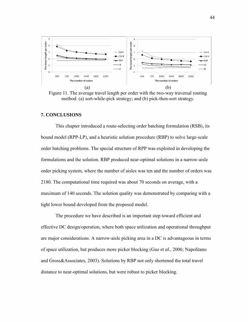
44
(a) (b)
Figure 11. The average travel length per order with the two-way traversal routing method: (a) sort-while-pick strategy; and (b) pick-then-sort strategy.
7. CONCLUSIONS
This chapter introduced a route-selecting order batching formulation (RSB), its
bound model (RPP-LP), and a heuristic solution procedure (RBP) to solve large-scale
order batching problems. The special structure of RPP was exploited in developing the
formulations and the solution. RBP produced near-optimal solutions in a narrow-aisle
order picking system, where the number of aisles was ten and the number of orders was
2180. The computational time required was about 70 seconds on average, with a
maximum of 140 seconds. The solution quality was demonstrated by comparing with a
tight lower bound developed from the proposed model.
The procedure we have described is an important step toward efficient and
effective DC design/operation, where both space utilization and operational throughput
are major considerations. A narrow-aisle picking area in a DC is advantageous in terms
of space utilization, but produces more picker blocking (Gue et al., 2006; Napolitano
and Gross&Associates, 2003). Solutions by RBP not only shortened the total travel
distance to near-optimal solutions, but were robust to picker blocking.

45
A variety of direct extensions of RBP are possible. We showed the RBP
framework was extendible to wide-aisle picking systems with a two-way traversal route.
Some order picking systems, such as a multiple cross-aisle system (Roodbergen and de
Koster, 2001) and a 2-block warehouse (Le-Duc and de Koster, 2007), can also be
modeled using the RBP batching procedure. In those systems, it is possible to enumerate
available or preferred routes (R) and to define matching relationships between routes and
orders (Or) for general situations. As long as the warehouse manager can construct a
preferred route set (R), the proposed algorithm can solve the problem with only slight
modifications.
Extending this research to consider other routing methods and to explicitly
account for picker blocking will be useful. First, the proposed procedure can be a key
enabler when developing an efficient batching algorithm with different routing methods
as discussed in Section 6.3. Second, picker blocking should be scrutinized and managed
in order picking operations. Our experimental results indicate that using the RBP method
for batching can have significant benefits in terms of reduced picker blocking. However,
productivity loss by picker blocking still remains an issue. These observations provide
motivation for the research described in the next chapters.

46
CHAPTER V
ANALYSIS OF PICKER BLOCKING IN NARROW-AISLE
BATCH PICKING
This chapter identifies sources of picker blocking in batch picking in a narrow-
aisle situation and determines satisfactory operational situations, e.g., batching algorithm,
sorting strategy, for reducing picker blocking. We present new multiple-pick analytical
models to more accurately evaluate picker blocking in a closed-form expression of pick
density and the number of pick faces. We compare the results developed from a
conventional single-pick order picking models to our multiple-pick models to quantify
and identify sources of picker blocking. Note a single pick model assumes there can be
at most one picker per pick face, whereas a multiple-pick model allows multiple picks at
a pick face. Finally, a simulation study over a variety of batching situations is presented.
We highlight three findings for narrow-aisle batch picking processes: 1) variation in
pick density across aisles affects picker blocking as much as the magnitude of pick
density; 2) a near-optimal distance-based batching algorithm can reduce picker blocking
when an appropriate sorting strategy is employed, because it reduces both the number of
aisles visited and the variation in the number of picks per aisle; and 3) the sorting
strategy (i.e., a pick-then-sort strategy or a sort-while-pick strategy) causes varying
amounts of congestion, depending on possible routing options used.
1. INTRODUCTION
We consider a narrow-aisle picking environment, which is very attractive for its

47
storage capability. However, the narrow-aisle configuration can produce picker blocking,
even though one-way traversal routing is used to mitigate congestion (Gue et al., 2006).
Accordingly, the order fulfillment time can lengthen and operational costs increase. In
practice, the effects of batch formation on picker blocking vary according to the batching
algorithm, sorting strategy, and storage policy.
A principle of batch picking is to have pickers gather items that are closely
located within the storage space when feasible. Basically, a batch has a higher pick
density compared to a single order, which leads to higher picker utilizations. Two studies
(Gue et al., 2006; Skufca, 2005) consider a model under a single-pick assumption
defined as a situation in which only a single product type is picked at a particular pick
face. However, in batch picking, the probability of needing to pick more than one
product type at a particular pick face increases. Thus, multiple-pick models that consider
repeated picks at a particular pick face can be useful. Parikh and Meller’s (2010) recent
analytical models of picker blocking considering multiple-picks in narrow-aisle
configurations begin to develop an understanding of the impact of non-deterministic pick
times as well as multiple-picks at a stop on order picking performance.
However, to date, researchers do not fully understand the relationship between
picker blocking and batch formation. Gue et al. (2006) and Parikh and Meller (2010)
have identified two sources of picker blocking as the size and variation of pick density.
However, the impact of batch formation on picker blocking has not been characterized.
It is evident that practical picking situations (i.e., batching algorithm, sorting strategy,
and storage policy) influence batch formation and thus can have differing effects on two

48
sources of picker blocking.
In general, an analytical model characterizing picker blocking with a closed-form
expression in terms of the number of pickers, k, is desirable. The k-picker model can
help researchers analyze the impacts of increasing the number of pickers. The closed-
form expression can suggest diverse numerical analysis over different operations without
the use of simulations. Available analytical studies (Gue et al., 2006; Parikh and Meller,
2009; Parikh and Meller, 2010; Skufca, 2005) develop models of two extreme cases:
pickers’ walk speed is infinite or slow. Neither model exists in practice, but they can
bound actual situations and provide an excellent understanding of picker blocking.
Parikh and Meller’s (2010) two-pickers multiple-pick analytical models for narrow-aisle
configurations raise two issues : 1) the analytical model for the slow walk speed case is
developed based on four combinations of pick and walk tasks of two pickers;
consideration of picking and walking states restricts the extension of the models as well
as increases the computational complexity; and 2) a closed-form expression for the
infinite walk speed case has not been developed; thus their experimental study does not
provide analytical measures of picker blocking for varying pick density. In other words,
similar to a simulation, the experimental study requires a computational calculation.
Note that our study has been conducted independently from Parikh and Meller’s recent
study, but both studies produce similar analytical models and address an identical
opinion which is relevant for the impacts of multiple-picks on picker blocking. Although
Parikh and Meller’s study was published first, we show the differences between two
results. From the standpoint of the analytical models, the differences described above

49
have been identified. In terms of the research aim, however, we focus on both
developing analytical models over multiple-pick situations, and also scrutinizing order
batch picking situations which can give throughput benefits in a narrow-aisle
configuration by satisfying the analytical results (Parikh and Meller cover only the
impacts by multiple-picks on picker blocking).
This chapter develops new analytical models of picker blocking considering
multiple-picks in narrow-aisle configurations, which are simpler compared to Parikh and
Meller (2010) and can facilitate the derivation of two closed-form equations for the
probability of being blocked. Further relevant convergence characteristics are addressed
from the two closed-form expressions. More importantly, we conduct simulation studies
over different batch picking situations to relate characteristics of the picking
environment and picker blocking to determine appropriate batching strategies for high
order picking throughput.
This chapter is organized as follows. Section 2 details the relevant order picking
literature and identifies new research opportunities. Section 3 defines a circular blocking
model. In Section 4, we derive new blocking models under the assumption of two-
pickers and multiple-picks per location. We apply the models to two extreme cases.
Relevant insights about the differences between the multiple-pick models and a single-
pick model and the impacts of the size of variation in batch size are discussed. Section 5
examines the relationship between analytical models and batching situations. Section 6
summarizes the findings and offers suggestions for future research.

50
2. LITERATURE SURVEY
Picker blocking analysis in parallel-aisle picking systems can be distinguished by
the aisle width, which defines the physical form of the system. A narrow-aisle system is
typically characterized by no-passing in an aisle. The picker blocking created by the no-
passing condition is termed in-the-aisle blocking. Skufca (2005) presents a k-picker
congestion model of a circular no-passing system in the case of infinite walk speed. Gue
et al. (2006) address two-picker congestion models of a parallel-aisle pick area
approximated by a circular no-passing system considering infinite and unit walk speeds.
In the unit walk speed, the unit walk time to pass a pick face is identical to the unit pick
time. They also conduct additional simulations to investigate picker behavior under more
practical walk speed assumptions. The authors focus on identifying the effects of ―pick
density‖ on picker blocking under the single-pick assumption. Their results indicate that
a batch picking strategy in narrow-aisle OPSs is advantageous when the pick density is
either very low or very high. Parikh and Meller (2010) find that picker blocking can also
be significant when the variation of the pick density is high. They develop two-picker
congestion models under extreme walk speed assumptions and investigate other
scenarios via a simulation study. A closed-form expression was only derived for the unit
walk speed scenario. Their unit speed Markov chain model is relatively complex
compared to our model. In addition, their analytical model over the infinite walk speed
scenario experiences a gap compared to our result which is independently conducted and
more clearly satisfies a common characteristic of picker blocking models. Both issues
will be discussed in Section 4.
51
A wide-aisle system experiences a different type of picker blocking, referred to
as pick face blocking. Parikh and Meller (2009) investigate analytical models under both
the single-pick and multiple-pick assumption. The multiple-pick model, which allows a
picker to repeatedly pick at a pick face, can reflect a more realistic situation. The authors
indicate that the variation of pick density plays a vital role in increasing picker blocking
and find that the wide-aisle picking systems can encounter significant pick face blocking
when multiple picks occur at a pick face. Their comparison of the two models points to
the equal importance of the variation of pick time as well as the variation in pick density.
Several comparison studies to select a best-performing batching algorithm (De
Koster et al., 1999; Ho and Tseng, 2006; Pan and Liu, 1995; Ruben and Jacobs, 1999)
have been conducted during the last two decades. However, most studies (De Koster et
al., 1999; Ho and Tseng, 2006; Pan and Liu, 1995) evaluate performance in terms of
travel distance; only Ruben and Jacobs (1999) study the relationship between picker
blocking and batching algorithms. The latter authors indicate that the level of congestion
is affected by the selection of batching procedures and storage policies, although they
don’t provide a clear rationale for the congestion. Through simulation studies, they find
that a turnover-based storage policy, where popular products with large demand are
stored based on shortest-possible travel retrieval, generates more congestion than family-
based, where higher-demand products are stored closer together, or random storage
policies. Their blocking model approximates congestion by splitting an aisle in two and
disallowing other pickers to access an occupied area. This type of unique control policy
leads to different levels of congestion compared to recent studies (Gue et al., 2006;

52
Parikh and Meller, 2009; Skufca, 2005).
Reviewing the available literature, we identify two critical issues with respect to
the expression and analysis of picker blocking. First, the multiple-pick picker blocking
models by Parikh and Meller (2010) are complex and inaccurate. To establish a Markov
property, their analytical model for the slow walk speed case requires four sub states of
the pick and walk tasks of two pickers; consideration of pick and walk states restricts the
extension of the models as well as increases the computational complexity. In addition
their model lacks a closed-form expression of infinite walk speed despite the fact that
this type of expression can facilitate additional analysis of picker blocking.
Second, no analytical studies have fully investigated the relationship with the
batching algorithm even though, in practice, the batching algorithm may change both the
pick density level and its variation. Ruben and Jacobs’s (1999) result fails to explain
picker blocking in connection with batching algorithms, and there is no clear theoretical
rationale for the congestion. Gue et al.’s (2006) notion, i.e., less picker blocking when
pick density is very low or very high, also requires additional investigation as Parikh and
Meller (2010) finds a higher picker blocking situation. Furthermore, since both Gue et al.
and Parikh and Meller do not conduct their studies on batch picking environments, their
results do not explain practical situations.
3. PROBLEM DEFINITION
3.1 Batch picking in narrow-aisle picking systems
In narrow-aisle picking systems, pickers circumnavigate one-way aisles to
retrieve items from shelves and place them in a cart as shown in Figure 12. When an
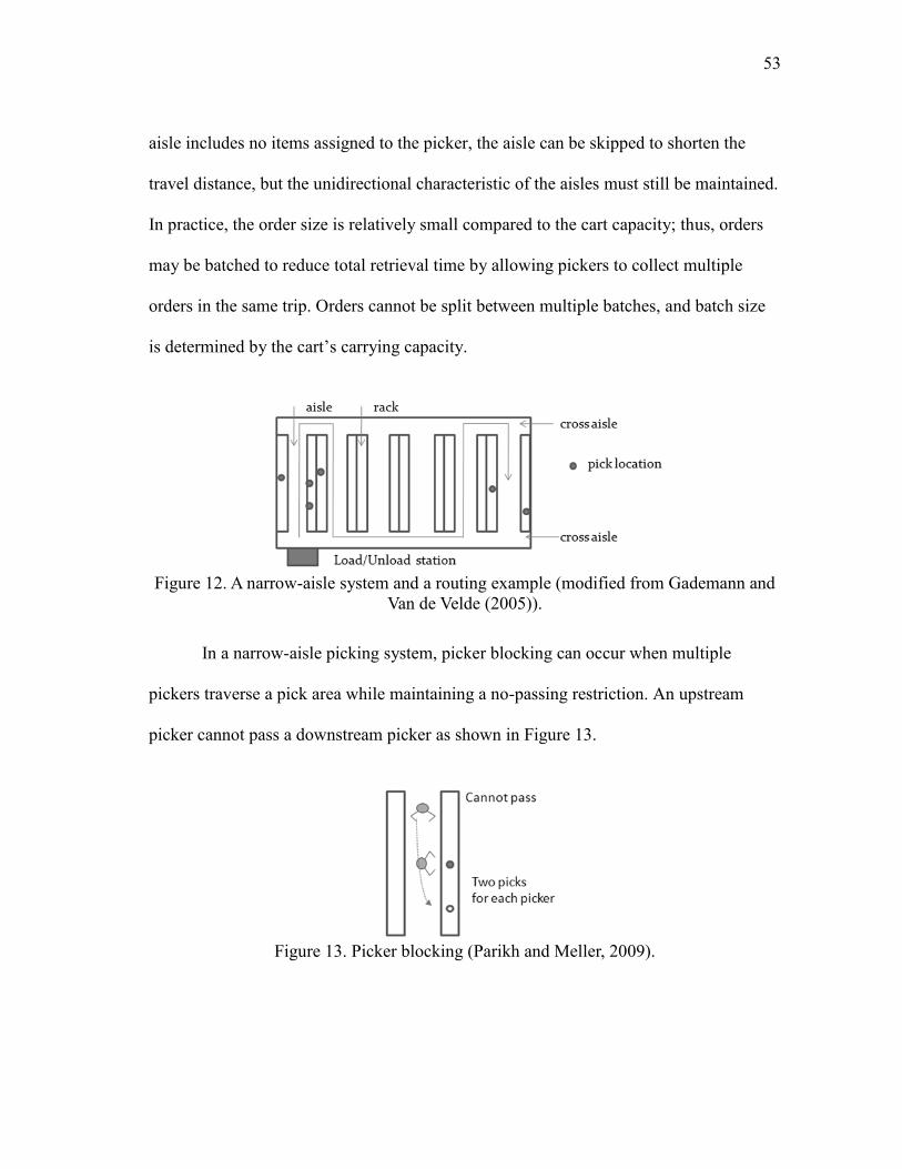
53
aisle includes no items assigned to the picker, the aisle can be skipped to shorten the
travel distance, but the unidirectional characteristic of the aisles must still be maintained.
In practice, the order size is relatively small compared to the cart capacity; thus, orders
may be batched to reduce total retrieval time by allowing pickers to collect multiple
orders in the same trip. Orders cannot be split between multiple batches, and batch size
is determined by the cart’s carrying capacity.
Figure 12. A narrow-aisle system and a routing example (modified from Gademann and
Van de Velde (2005)).
In a narrow-aisle picking system, picker blocking can occur when multiple
pickers traverse a pick area while maintaining a no-passing restriction. An upstream
picker cannot pass a downstream picker as shown in Figure 13.
Figure 13. Picker blocking (Parikh and Meller, 2009).
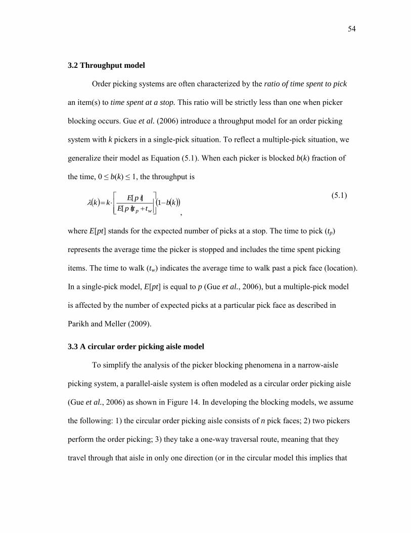
54
3.2 Throughput model
Order picking systems are often characterized by the ratio of time spent to pick
an item(s) to time spent at a stop. This ratio will be strictly less than one when picker
blocking occurs. Gue et al. (2006) introduce a throughput model for an order picking
system with k pickers in a single-pick situation. To reflect a multiple-pick situation, we
generalize their model as Equation (5.1). When each picker is blocked b(k) fraction of
the time, 0 ≤ b(k) ≤ 1, the throughput is
kbttp tE
p tEkk
wp
1
][
][
,
(5.1)
where E[pt] stands for the expected number of picks at a stop. The time to pick (tp)
represents the average time the picker is stopped and includes the time spent picking
items. The time to walk (tw) indicates the average time to walk past a pick face (location).
In a single-pick model, E[pt] is equal to p (Gue et al., 2006), but a multiple-pick model
is affected by the number of expected picks at a particular pick face as described in
Parikh and Meller (2009).
3.3 A circular order picking aisle model
To simplify the analysis of the picker blocking phenomena in a narrow-aisle
picking system, a parallel-aisle system is often modeled as a circular order picking aisle
(Gue et al., 2006) as shown in Figure 14. In developing the blocking models, we assume
the following: 1) the circular order picking aisle consists of n pick faces; 2) two pickers
perform the order picking; 3) they take a one-way traversal route, meaning that they
travel through that aisle in only one direction (or in the circular model this implies that

55
they move only in a clockwise direction); 4) pick time is constant regardless of the pick
face characteristics, such as shelf height; 5) at a pick face, pickers pick with a probability
p; q denotes 1-p, the probability of walking past a pick-face; 6) a picker can only be
picking, walking, or standing idle due to blocking; 7) the pick time and the walk time
between two pick faces are deterministic, termed as tp and tw, respectively.
Figure 14. A circular order picking aisle (Gue et al., 2006).
As a performance measurement, we obtain the percentage of time blocked,
denoted as bmpt:wt(k), where m stands for a multiple-pick situation and pt:wt represents
the pick:walk time ratio. In the case of a single-pick situation (s), Skufca (2005)
previously derived the analytical model for bs1:0(k). Gue et al. (2006) studied single-pick
models, i.e., bs1:1(2) and bs
1:0(2), analytically, and generalized to other cases (e.g.,
bs1:0.5(2), bs
1:0.25(2),…, bs1:1(10)) using simulation models. Parikh and Meller (2010)
conducted another study for multiple-pick models (bm1:1(2) and bm
1:0(2)), where the
analytical model for bm1:1(2) is presented in a closed-form expression using a discrete
Markov chain with 4(n-1) states, and bm1:0(2) is built on (n+1) state Markov chain, but
does not have a closed-form expression.

56
3.4 Scope of study
We wish to develop new analytical models for bm1:1(2) and bm
1:0(2) 5 and to
investigate the more general case bmpt:wt(k) over varying pick density variation, e.g.,
different pick density functions, using a simulation study in a circular order picking aisle.
For a more complete understanding of picker blocking and batch picking and their
relationships to other aspects of warehouse operations, we conduct an extended
simulation study considering batching algorithms, sorting strategies, and storage policies
in a parallel-aisle picking system.
4. ANALYSIS OF PICKER BLOCKING
We first build analytical models for two order pickers who conduct a retrieval
operation in a parallel-aisle picking system using the circular aisle characterization to
develop a general understanding, and then conduct a simulation study to reinforce the
significance in more practical situations.
Our analytical study considers two extreme cases that do not exist in practice but
provide bounds for realistic situations as well as help provide an excellent understanding
of picker blocking: 1) walk speed is equal to unit pick time per pick face (pick:walk time
= 1:1); and 2) walk speed is infinite (pick:walk time = 1:0). Our analytical model
utilizes a Markov property in determining distances between two pickers, which is
consistent with prior work, see also (Gue et al., 2006; Parikh and Meller, 2009; Skufca,
2005).
5 Our models replace and correct the Markov chains in Parikh and Meller (2010). First, we
introduce a new Markov chain independent of picking or walking information in the infinite walk speed case. Second, we present an accurate Markov chain model to derive a closed-form expression of the unit walk speed case.
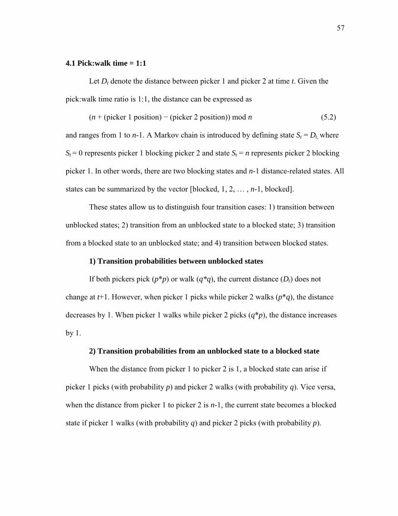
57
4.1 Pick:walk time = 1:1
Let Dt denote the distance between picker 1 and picker 2 at time t. Given the
pick:walk time ratio is 1:1, the distance can be expressed as
(n + (picker 1 position) − (picker 2 position)) mod n (5.2)
and ranges from 1 to n-1. A Markov chain is introduced by defining state St = Dt, where
St = 0 represents picker 1 blocking picker 2 and state St = n represents picker 2 blocking
picker 1. In other words, there are two blocking states and n-1 distance-related states. All
states can be summarized by the vector [blocked, 1, 2, … , n-1, blocked].
These states allow us to distinguish four transition cases: 1) transition between
unblocked states; 2) transition from an unblocked state to a blocked state; 3) transition
from a blocked state to an unblocked state; and 4) transition between blocked states.
1) Transition probabilities between unblocked states
If both pickers pick (p*p) or walk (q*q), the current distance (Dt) does not
change at t+1. However, when picker 1 picks while picker 2 walks (p*q), the distance
decreases by 1. When picker 1 walks while picker 2 picks (q*p), the distance increases
by 1.
2) Transition probabilities from an unblocked state to a blocked state
When the distance from picker 1 to picker 2 is 1, a blocked state can arise if
picker 1 picks (with probability p) and picker 2 walks (with probability q). Vice versa,
when the distance from picker 1 to picker 2 is n-1, the current state becomes a blocked
state if picker 1 walks (with probability q) and picker 2 picks (with probability p).

58
3) Transition probabilities from a blocked state to an unblocked state
If picker 1 is blocked by picker 2, picker 1 must wait for picker 2 to walk (with
probability q) to exit a blocked state. Vice versa, when picker 2 is blocked by picker 1,
picker 2 must wait for picker 1 to walk (with probability q).
4) Transition probabilities between blocked states
When the current state is blocked, a pick can occur with probability p and the
blocking status remains, i.e., a blocked state transitions to a blocked state with
probability p.
In sum, when multiple picks are allowed, the transition probabilities can be
described in a transition diagram as illustrated in Figure 15.
Figure 15. State space and transitions for the Markov chain model when picking time equals travel time.
The Markov chain model in Figure 15 does not include substates of picking or
walking as the Gue et al. (2006) and Parikh and Meller (2010) models. Thus the
transition matrix is more condensed. The resulting transition matrix, which has
dimensions (n+1) x (n+1), is:

59
pq
pqqppq
pqqp
qppq
pqqppq
qp
A
0000
000
000
000
000
0000
22
22
22
22
Stationary distribution
We obtain the following v, which satisfies vA = v.
1,
1,,
1,1
ppv
The stationary density using ||v|| is scaled to obtain a stationary probability. From
v above, this implies:
p
n
pnv
12
1112
The blocking probability of one picker at one blocked state is
121
2
12 *1
1:1
np
p
p
nv
vb m (5.3)
Equation (5.3) is identical to the results by Parikh and Meller (2010), whose
transition matrix has dimensions 16*(n-1) x (n-1). Figure 16 plots percentage of time
blocked over different number of aisles (n). The 1:1 picker blocking model estimates a
smaller productivity loss when the picking area includes more pick faces as shown:

60
Figure 16. The percentage of time that pickers are blocked over different number of pick faces when two pickers work with pick:walk time = 1:1.
Productivity loss over pick density starts from 0, increases as pick density
increases, and converges to 1/(n+1) as pick-density approaches 1. This result is
summarized in the following theorem.
Theorem 1. When two pickers travel at unit speed, the percentage of time
blocked is at least 0 and at most 1
1
n .
Proof. (5.3) is a monotonic increasing function. Its limiting value is 0 when p
goes to 0 and 1/(n+1) when p goes to 1 as follows: 012
lim0
pn
p
p,
1
1
12lim
1
npn
p
p. The result is
1
1% blocked time0
n. End of proof.
Figure 17 compares the relationship between a multiple-pick (m) model and a
single-pick model (s) over two different numbers of pick faces (20 and 50 pick faces).
Here, the x-axis is the average number of picks, not pick density. As Equation (5.1)

61
indicated, the throughput comparison over identical workloads (i.e., the number of picks)
can express the impact of picker blocking. The multiple-pick results are monotonically
increasing, while the single-pick results, developed by Gue et al. (2006), show a drop in
picker blocking at high pick requirements.
Figure 17. The comparison of single-pick and multiple-pick models when two pickers work with pick:walk time = 1:1.
Note that the proposed discrete-time Markov chain of picker blocking for
multiple-picks with a pick:walk time = 1:1 differs from Parikh and Meller (2010) in that
the distance is not conditioned on the operation modes of the pickers (i.e., walking or
picking). As we addressed above, when multiple-picks are allowed, a Markov property
of distance holds regardless of the previous walking or picking status. The conditional
multiple-pick model is summarized in Appendix B.1, which is similar to the Parikh and
Meller (2010) model. Moreover, the approach described in this chapter is applicable in
wide-aisle systems discussed in Parikh and Meller (2009) (see Appendix B.2).
4.2 Pick:walk time = 1:0
The infinite speed assumption allows for transitions to multiple states in our
62
Markov chain model. Thus, the probability that a picker moves distance x is
approximated, and then a probability function for the distance y, characterizing the
change in the distance between the two pickers, is estimated.
Let random variables X1t and X2
t represent the number of locations moved in time
t by pickers 1 and 2, respectively. If a picker picks more than one pick at a pick face, the
distribution of the location is defined over the infinite sample space with a random
variable characterizing the number of locations between two pickers:
,...2,1,0 for xpqxf x . (5.4)
Yt = X1t - X2
t denote the change in distance between the two pickers when passing
is not allowed. As described in Appendix B.3, the probability density function of Yt (g(y))
becomes:
yq
pqyg
y
-for 1
(5.5)
Suppose the distance at the previous state is Dt−1 = r. The actual change in
distance is bounded by the physical blocking phenomenon and the amount of the change
is limited by r. Like the previous 1:1 analysis, four transition cases are defined: 1)
transition between unblocked states; 2) transition from an unblocked state to a blocked
state; 3) transition from a blocked state to an unblocked state; and 4) transition between
blocked states.
1) Transition probabilities between unblocked states
In this case, the distribution function (5.5) is used directly. Given r, the change is
bounded between 1 and n-1 ruling out the possibility of the first picker catching up to the

63
second picker.
1,...,1,1-1for 1
nrrnyrq
pqyYP
y
t
2) Transition probabilities from an unblocked state to a blocked state
The next step is calculating the probability of events with blocking. To obtain
this probability, we need to accumulate all cases above the limits (0 or n). We note that
there will be blocking at state 0 if Yt ≤ −r. g(y) is symmetric and the probabilities for the
bounding cases are calculated as:
11for ,
1
1
1
1
1
nr q
q
q
p
q
pqrYP
rr
ry
y
t
11for ,1
nr q
qrnYP
rn
t
3) Transition probabilities from a blocked state to an unblocked state
The distribution function (5.5) is again used directly. Note that r is 0 or n when a
picker is blocked. Since the blocked picker walks first, initially, the distance between
two pickers also becomes 0 or n.
nrrnyrq
pqyYP
y
t or 0,1-1for 1
4) Transition probabilities between blocked states
Similar to 3), r = 0 or n express the blocked states. Without loss of generality, the
probabilities in 2) are applicable. Thus, expressions for both the lower bound and the
upper bound are as follows:
or 0for ,
1 nr
q
qrYP
r
t

64
or 0for ,
1 nr
q
qrnYP
rn
t
The probabilities that we derive are similar to Parikh and Meller (2010) with one
exception. While managing the transition from blocked (0) to blocked (n) or blocked (n)
to blocked (0), the equation above uses )1( qqn from the transition probability 4),
which differs from )1(2 qqn in Parikh and Meller. Since they do not offer any
comment on both values, the reason cannot be identified. Instead, we use a
computational comparison, which will be discussed later.
The result forms the following transition matrix:
pq
q
pq
q
pq
q
pq
q
q
q
q
q
p
q
pqpqpq
q
q
q
q
q
pqpq
q
q
q
q
q
pq
q
pq
q
q
q
q
q
pq
q
pq
q
pq
q
p
q
q
q
q
q
pq
q
pq
q
pq
q
pq
q
A
nnn
nnn
nn
nn
nnn
nnn
1
1
11111
111111
1111
1111
111111
111111
1
221
321
232
232
123
122
Stationary distribution
To identify a stationary distribution, a v which satisfies vA = v is identified as:
1,,...,,1 ppv
We can scale the stationary density using ||v|| = 2+(n-1)p. The blocking
probability of a picker at one blocked state is:

65
pn
bm
12
120:1
(5.6)
Because of the differences in the expression for the transition probabilities from
blocked (0) to blocked (n) or blocked (n) to blocked (0), the results given by the 1:0
analytical model we propose have a 0.032 to 0.170% error gap compared to the results
from Parikh and Meller’s (2010) model. According to Parikh and Meller (2009), when p
= 1, both 21:1mb and 20:1
mb should converge to the same value regardless of walk speed.
A high pick density leads to the same congestion situation, which is observed in single-
pick narrow-aisle models (Gue et al., 2006) and wide aisle models (Parikh and Meller,
2010). When p=1, the equation in our 1:0 analytical model satisfies the general
knowledge, but Parikh and Meller’s model experiences a gap of 0.0083% when the
number of pick faces = 20.
As the function is derived, the convergence characteristic of the 1:0 model can be
investigated, and the following theorem is observed.
Theorem 2. When two pickers travel at infinite speed, the percentage of time
blocked is at most 50% and at least 1
1
n.
Proof. (5.6) is a monotonic decreasing function. There are two limiting
characteristics. As p goes to 0, the upper limiting value is 2
1
12
1lim
0
pnp. The
lower limiting value is 1/(n+1) as follows: 1
1
12
1lim
1
npnp.

66
The result is 2
1 % blocked time
1
1
n. End of proof.
Figure 18 depicts the productivity loss over different numbers of pick faces.
Picker blocking starts from picker utilization 50%, decreases as pick-density increases,
and converges to 1/(n+1). As we observed in the 1:1 model, larger areas are less
susceptible to picker blocking than smaller areas.
Figure 18. The percentage of time that pickers are blocked over different number of pick faces when two pickers work with pick:walk time = 1:0.
Figure 19 compares a multiple-pick (m) model and a single-pick model (s) over
20 pick faces and 50 pick faces. The percentage of time blocked for both the multiple-
pick and single-pick models decreases monotonically as pick density increases. However,
the multiple-pick results consistently experience a higher percentage of time blocked.
Moreover, as Equation (5.6) indicated, the percentage of time blocked for the multiple-
pick model goes to 1/(n+1), not to 0.

67
Figure 19. The comparison of single-pick and multiple-pick models when two pickers work with pick:walk time =1:0.
From theorems 1 and 2, a further important result can be derived.
Theorem 3. As pick density goes to 1, the percentage of time blocked converges
to 1
1
nwhen there are two pickers.
Proof. This proof is a direct extension of the previous results. When the walk
speed is equal to the pick time, we can use Equation (5.3) as follows:
1
1
12lim
1
npn
p
p. When pickers walk at infinite speed, Equation (5.6) experiences
the same convergence: 1
1
12
1lim
1
npnp. End of proof.
4.3 Simulation study
The two analytical models are based upon three assumptions: 1) extreme
pick:walk time ratio; 2) a Markov property in distance between pickers; and 3) the
68
circular approximation to a parallel aisle order picking area. Below, assumptions 1 and 2
will be relaxed and investigated via a simulation study; assumption 3 will be maintained
in Sections 4 and 5. Appendix B.4 discusses the validation of our analytical models and
simulations by cross comparison among our analytical models, our simulation models,
and Parikh and Meller’s (2010) results.
4.3.1 Fractional walk speed
In practice, pickers are not extremely fast or slow. If the pick time is 1, most
practical speeds for walking are on the range [0.05,1] (Gue et al., 2006). For example,
our literature review found a fast speed would have a pick to walk ratio of 1:0.1
(Petersen, 2000) and a slow speed would have a ratio of 1:0.2 (Yu and De Koster, 2009).
We conduct a simulation study with pick:walk time = 1:0.025, 1:0.05, 1:0.1, 1:0.2, and
1:0.5. Figure 20 illustrates the simulations’ results of a two-picker model (labeled a) and
a five-picker model (labeled b). Solid lines are the results with pick:walk time = 1:0,
1:0.025, 1:0.05, 1:0.1, 1:0.2, 1:0.5, and 1:1 from top to bottom. The upper dotted line is
an analytical result with pick:walk time = 1: 0. The lower dotted line is an analytical
result with pick:walk time = 1:1.
As pick density increases, the percentage of time blocked converges to
approximately the value derived in Theorem 3. For example, when p = 0.95, in Figure 20
(a) ranges [4.53, 5.00] of throughput loss by picker blocking in a 20-pick face circular
picking system with two pickers. According to Theorem 3, the loss is 1/21 = 4.76 when
two pickers are in the order picking system. Figure 20 (b), using five pickers, converges
to [3.79, 3.86]. Our observation indicates that the multiple-pick characteristic of batch

69
picking increases picker blocking. In addition, picker blocking is an issue regardless of
variation of pick density in a narrow-aisle order picking. This result supports the
observations of Parikh and Meller (2010) in a narrow-aisle order picking and Parikh and
Meller (2009) in a wide-aisle order picking.
(a) (b)
Figure 20. The percentage of time blocked over different pick:walk time ratios: (a) two pickers in 20 pick faces; and (b) five pickers in 100 pick faces.
4.4.2 Non-Markov property in distance: Variation of the number of picks
In multiple-pick and single-pick analytical models, the number of picks in a trip
(from the first pick face to the last pick face) is determined to maintain a Markov
property of the distance between two pickers. That restriction is relaxed and investigated
via simulation. A simulation model developed with the same pick probability restrictions
as the single-pick analytical model (Gue et al. (2006)) is used. Several models are
considered: a simulation model generated with the restrictions in the multiple-pick
analytical model (described above), a fixed-size model (the number of picks in a trip is
constant), and a uniform-size model (the number of picks in a trip follows a discrete
uniform distribution [mean/2, mean *3/2]).
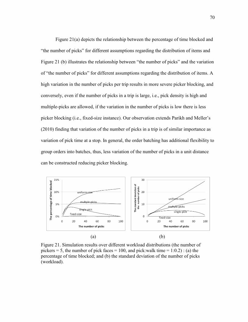
70
Figure 21(a) depicts the relationship between the percentage of time blocked and
―the number of picks‖ for different assumptions regarding the distribution of items and
Figure 21 (b) illustrates the relationship between ―the number of picks‖ and the variation
of ―the number of picks‖ for different assumptions regarding the distribution of items. A
high variation in the number of picks per trip results in more severe picker blocking, and
conversely, even if the number of picks in a trip is large, i.e., pick density is high and
multiple-picks are allowed, if the variation in the number of picks is low there is less
picker blocking (i.e., fixed-size instance). Our observation extends Parikh and Meller’s
(2010) finding that variation of the number of picks in a trip is of similar importance as
variation of pick time at a stop. In general, the order batching has additional flexibility to
group orders into batches, thus, less variation of the number of picks in a unit distance
can be constructed reducing picker blocking.
(a) (b)
Figure 21. Simulation results over different workload distributions (the number of pickers = 5, the number of pick faces = 100, and pick:walk time = 1:0.2) : (a) the percentage of time blocked; and (b) the standard deviation of the number of picks (workload).

71
5. COMPARISON STUDY IN PARALLEL-AISLE PICKING SYSTEMS
Another difficulty encountered when analyzing picker blocking in real picking
situations arises due to the multiple-aisles characteristic and impacts by routing. In this
section we describe an extended simulation study in a parallel-aisle order picking system.
In particular, in a parallel-aisle order picking system with multiple aisles, decreasing the
travel distance is a primary concern of management. Thus, a batching algorithm to
efficiently reduce the travel distance is developed. In addition, a sorting strategy and a
storage policy often are changed to maximize the retrieval performance (Frazelle, 2002;
Tompkins et al., 2003). The batching algorithm, sorting strategy, and storage policy can
increase the expected number of picks at a stop, but they also impact picker blocking
(b(k)). This section describes the effects of the batching algorithms, sorting strategies,
and storage polices on picker blocking.
5.1 Simulation design
Various batching algorithms are available. Specifically, large-scale order
batching situations will be considered, thus the comparison is limited to those that can
handle large problems sizes. From the available literature, the following are considered:
Seed: the seed algorithm developed in De Koster et al. (1999): 1) select a
seed having the largest number of aisles; 2) choose the order minimizing
the number of additional aisles; and 3) update the seed as an order is added
to it.
CW II: the Clarke and Wright algorithm (II) in De Koster et al. (1999). See
Appendix B.5 for more detail.
RBP: the heuristic route-selection-based batching algorithm. See Chapter
IV and Appendix B.6 for more detail.
72
Seed and Clarke and Wright (CW) II are identified as the best algorithms in de
Koster et al.’s comparison study (1999). The route-selection batching procedure (RBP)
is a near-optimal batching algorithm discussed in Chapter IV.
A sorting strategy impacts the batching algorithms by affecting the units of
measure determining the batch size. Basically, the pickers carry bins or boxes on the cart
to store each order separately in a ―sort-while-pick‖ operation. Thus, the batch size is
determined by the number of bins, i.e., the number of orders. Another strategy, ―pick-
then-sort‖, does not carry bins (but it does require a sorting operation after the
completion of the picking operation). In this case, the picker does not need to carry bins
and separate orders, rather he/she can mix orders on the cart and orders can be batched to
maximize capacity.
Products are typically stored in warehouses to minimize retrieval efforts. In
general, a class-based storage policy stores the more frequently requested items closest
to the loading station to reduce the trip distance in contrast to a random storage policy
where items are stored in random locations in the warehouse.
Consider a general order picking situation: the number of orders in a time
window = 540 orders, eight time windows per shift, pick:walk time ratio = 5:1, setup
time per batch = 0, average order size = two items (uniform [1,3]), five pickers, and cart
capacity = 10 orders when sort-while-pick strategy and 20 items when pick-then-sort
strategy. A two-aisle system and a ten-aisle system with identical total number of pick
faces as 100 are considered to investigate the effects of pick density. While the two-aisle
system is similar to a circular aisle model, the ten-aisle system captures the effects that

73
asiels can be skipped as long as the one-way travel within aisles is maintained. The
number of simulation runs per instance (i.e., 20 runs per instance) following Ruben and
Jacobs (1999). The percentage of time blocked and the standard deviation of the number
of picks in an aisle (STD) are compared across scenarios.
5.2 Experimental results
Figure 22 shows the total travel distance and the total retrieval times for eight
different situations, while Figure 23 depicts the productivity loss for each batching
algorithm. The two-aisle instances of FCFS in Figure 23 (a) is very similar to Gue et al.
(2006). The productivity loss is approximately 1~3%. In the two-aisle models, other
batching algorithms have similar or slightly better picker utilization, because there is a
very small reduction of the total travel distance by decreasing the number of trips.
In the ten-aisle instances, the FCFS procedure in Figure 23 (a) shows a small
percentage of time blocked, approximately 1.5~4.2%. However, with respect to overall
performance, other batching algorithms achieve significantly larger reductions in the
travel distance (Figure 22 (a)) and overall throughput improvement which is inversely
related to the total retrieval time shown in Figure 22 (b). For batching algorithms other
than FCFS, a productivity loss by picker blocking becomes an issue as noted by
discussed in Section 4.3 and Parikh and Meller (2010).

74
(a)
(b)
Figure 22. Comparison over different batching algorithms of: (a) total travel distance; and (b) total retrieval time.

75
(a)
(b)
(c)
(d)
Figure 23. The percentage of time blocked and standard deviation of the number of picks per aisle over different batching algorithms: (a) FCFS; (b) seed; (c) CW II; and (d) RBP.

76
The results of the experiments provide insights regarding batching algorithms,
sorting strategies, and storage policies as follows:
1) Solution quality of batching algorithm impacts picker blocking when an appropriate
sorting strategy is employed.
The seed algorithm creates heavy congestion compared to FCFS, because the
algorithm increases pick-density. CWII shows less picker blocking compared to the seed
algorithm. However, the RBP solution exhibits less congestion due to reduced travel
distance. Furthermore, the standard deviation of RBP is less than the standard deviation
of the seed algorithm, and is less or a little more than the standard deviation of the CW II
algorithm. Intuitively, an improved distance-based batching algorithm could encounter
more congestion. However, RBP reduces congestion due to large reductions in the
distance traveled, and relatively reasonable variation of picks per aisle as shown in
Figure 23.
2) Sorting strategy impacts picker blocking when combined with RBP.
When the sorting operation is combined with an appropriate OPS size (i.e., the
number of aisles) and as the solution quality of batching algorithms is close to optimality,
e.g., RBP in most scenarios and CW II in a few particular cases, a distance-based
batching model performs well in terms of picker blocking. In the two-aisle picking
system with a single route, the pick-then-sort strategy experiences less picker blocking
as shown in Figure 23 (d). Vice versa, in the ten-aisle pick system characterized by
several routing lengths ((five cases of number of aisles visited: 2, 4, 6, 8, and 10), the
sort-while-pick strategy is advantageous (see Figure 23 (d)).

77
In the two-aisle picking system, only single route is available under the traversal
routing method. The pick-then-sort strategy determines the batch size by the number of
picks. Then, the variation of picks across batches is 0 if batches are consolidated
optimally. Accordingly, the variation of picks per aisle is 0, which is similar to a ―fixed-
size‖ case (see Section 4.4.2). Thus, RBP reduces picker blocking, whereas the sort-
while-pick strategy packs each batch with a constant number of orders. Thus, the number
of picks across batches can vary within range of the batch size * the order size. The sort-
while-pick strategy results in greater picker blocking compared to the pick-then-sort
strategy in the two-aisle picking situation.
The ten-aisle picking system faces a different situation as the number of aisles
visited across batches becomes diverse. When the sorting operation is separated from the
order picking operation (pick-then-sort strategy), there is more variation of the number
of picks per aisle across batches. Intuitively, a batch should contain the same number of
items, but the number of aisles visited is not identical. Thus, the variation of the number
of picks per aisle among batches varies widely, as do the route lengths.
In the sort-while-pick strategy, less variation of picks per aisle can be achieved
while obtaining a high quality solution. The sort-while-pick strategy constrains each
batch to have the same number of orders, not number of items. A batch with a long route
may include orders passing more aisles. To pass more aisles, each order may contain
more items. Then, the batch with a long route may include more items because the batch
size is determined by the number of orders, and vice versa. In conclusion, the expected
number of picks of a batch will typically be proportional to the length of route, i.e., the

78
number of aisles visited, as batches are packed more optimally. Thus, compared to the
pick-then-sort strategy, this characteristic can produce less variation of the number of
picks per aisle, which reduces picker blocking.
3) Similar to Ruben and Jacobs (1999), class-based storage policies increase picker
blocking.
When a class-based storage policy is applied, picker blocking increases as Ruben
and Jacobs observed. Even though the RBS algorithm implements a sort-while-pick
strategy (Figure 23 (d)), the productivity loss due to congestion is 7.5%. In other words,
the class-based storage policy offsets the gain of the travel distance with the losses
related to picker blocking as shown in Figure 22. The previous observation (impacts by
near-optimality and sorting strategy) is still valid since each aisle stores items evenly
under the class-based storage policy.
6. CONCLUSION AND FURTHER STUDY
This chapter provided a new understanding of picker blocking in a narrow-aisle
batching picking situation and scrutinized the relationship between picker blocking and
order batching using both analytical models and simulation studies. New analytical
models of two specific conditions in two-picker order picking situations (a slow walk
speed and an infinite walk speed) are developed. Specifically, two closed-form
expressions were derived and the relevant convergence characteristics addressed.
Diverse simulations were conducted varying several warehouse policies including the
batching algorithm, the sorting strategy, and the storage policy. Most importantly,
simulation results showed that a near-optimal distance-based batch algorithm (RBP)

79
creates very little picker blocking. Furthermore, the sorting strategy affects the variation
of the number of picks in an aisle, thus making specific sorting strategies (sort-while-
pick) more effective in large facilities.
These experimental results reveal that batch strategies faces different levels of
picker blocking and identify the conditions under which blocking can be reduced. First,
we verified the importance of pick density on picker blocking (Parikh and Meller, 2010).
Second, the distance-based batching (RBP) algorithm lessened picker blocking, because
of a very significant reduction in the travel distance and a relatively uniform pick density.
Third, a sort-while-pick strategy induces less picker blocking when a RBP was used in a
large facility.
80
CHAPTER VI
BATCH PICKING IN NARROW-AISLE ORDER PICKING SYSTEMS WITH
CONSIDERATION FOR PICKER BLOCKING
Reducing the time spent picking orders benefits warehouse operations by
decreasing the resources required and by improving response time. The two primary
components of the time spent picking orders are traveling time and blocking time. This
chapter proposes a batching and sequencing procedure called the indexed batching
model (IBM) with the objective of minimizing an aggregation of travel distance and
congestion delay. The IBM differs from the traditional batching formulation in that it
assigns orders to indexed batches, where a batch index represents the batch’s release
sequence. A mixed integer programming solution for exact control is developed and a
simulated annealing procedure for a large-scale environment is demonstrated. Our
results indicate that the integrated batching-and-sequencing approach achieves the
throughput improvement not realized by the traditional approaches and allows for the
development of batch picking strategies that are ideal for narrow-aisle order picking
systems.
1. INTRODUCTION
DCs are constantly challenged to reduce the cost of their operations and to
become more efficient. One common way to lower costs per unit shipped is to increase
space utilization (Napolitano, 2009). According to the recent warehouse operations
survey (Napolitano, 2008), the warehousing industry has three major cost sources:

81
inventory, investment, and order processing. For example, rising inventories often force
warehouses to store more goods in less space (Gue et al., 2006; Napolitano, 2009).
Narrow-aisle picking systems are one alternative to increase space utilization with
minimal investment costs. However, the narrow-aisle characteristic can add to order
picking costs due to longer travel and more congestion (Gue et al., 2006). Small order
sizes exacerbate the problem, because they require more trips through the picking area.
Implementing an efficient batch order picking strategy can help to reduce operational
costs in a narrow-aisle order picking environment with small order sizes.
However, the combination of narrow-aisle OPS and a batch picking strategy can
suffer from significant operational performance loss and control difficulties related to
picker blocking (Gue et al., 2006; Parikh and Meller, 2010). As more pickers travel in a
picking area, well-designed control policies can reduce travel distances or improved
design of the facility may elevate these congestion issues (Zhang et al., 2009).
Traditionally, an OPS can be designed with wide aisles to create less blocking, or can be
operated using zone picking, where each zone contains a single picker. However, both of
these approaches are not viable in many cases due to additional space (or cost)
requirements.
Other approaches employ routing alternatives. Zhang et al. (2009) provide an
alternative routing method where the path is dependent on the congestion amount. Gue
et al. (2006) briefly introduce a routing strategy where a downstream (= blocking) picker
exits an aisle and circulates back behind an upstream (blocked) picker using an empty
aisle when there is significant congestion. However, the alternative paths or averted

82
routing approaches may lengthen a trip compared to the original route, and can be
challenging to implement in practice.
Control policies to trade off travel distances and time blocked have not been
addressed in the academic literature. Thus, the goals of this chapter are: 1) develop a
control framework combining order batching and sequencing issues; 2) present a
practical solution procedure to solve the integrated batching and sequencing problem;
and 3) vary the order picking environments to investigate the performance of the
proposed strategy. A new batching framework is developed including the sequencing
problem. The proposed model is formulated as a mixed integer program (MIP). This
formulation can only be solved optimally for small size problems. To overcome this
limitation, we adapt a simulated annealing heuristic approach.
The chapter is organized as follows. Section 2 briefly reviews related studies. In
section 3, a concise batching framework to handle blocking is developed. The
framework considers a picking area with one-way aisles and uses insights from flow-
shop scheduling problem to identify strategies to reduce picker blocking. Section 4
develops an indexed batching framework to address in-the-aisle picker blocking. Section
4 also addresses the sequencing of batches, how the multiple aisle impacts the
framework, and how the proposed model can handle multiple trips. In Sections 5 and 6,
we formulate a MIP and develop a simulated annealing heuristic solution approach,
summarize the results, and discuss the importance of the findings.
2. LITERATURE SURVEY
When operational costs due to picker blocking are excessive, engineers prefer

83
alternative OPS configuration or order picking strategy to control blocking. Alternatives
are available for a wide-aisle OPS (Parikh and Meller, 2009) or in the case of zone order
picking (De Koster and Yu, 2008). However, for facilities in which space is a concern
changing the layout and order picking operations to either of these alternatives may not
be feasible. Further, to make the best use of their limited space some warehouses have
narrow-aisles. However, if picker blocking is a concern in these settings the only
solutions available in the literature are passing and rerouting strategies (Gue et al., 2006;
Zhang et al., 2009). We review the previous studies of OPSs focusing on picker blocking.
To structure our review of the related studies, each is classified based on their modeling
methodology as: 1) analytical models of picker blocking; 2) routing methods with picker
blocking; and 3) picker blocking while batching orders.
Gue et al.(2006) and Parikh and Meller (2009) introduce analytical models to
quantify narrow-aisle and wide-aisle picker blocking, respectively. They determine the
relationship between throughput and pick density demonstrating the significance of
picker blocking. The results indicate that batch picking strategies in narrow-aisle OPS
are advantageous when the pick density is either very low or very high (Gue et al., 2006).
The problem of controlling or reducing picker blocking while routing has rarely
been studied. Ratliff and Rosenthal (1983) present a polynomial timed dynamic model to
optimally solve the order picking problem when the objective is to minimize travel
distance. Hall (1993) surveys heuristics routing for practical purposes, and concludes
that S-shape and largest-gap strategies are reasonable strategies for minimizing travel
distance. These studies attempt to minimize travel distance, but when an order picking

84
area has significant traffic, picker blocking may result in additional distance traveled or
time penalty; a structured analysis of additional travel distance or time delays is omitted
in the literature. Gue et al.(2006) discuss practical methods to avoid picker blocking,
such as allowing a trailing picker to pass while the leading picker unload collected items,
or forcing a blocked picker to exit the current aisle and use an empty aisle to continue to
traverse the pick area when significant blocking is expected.
Moreover, some literature indicates that batch picking tends to face less picker
blocking. Gue et al. (2006) introduce an industry case with less picker blocking when
pick density is very high. Ruben and Jacobs (1999) show the relationship between the
batching algorithm and the storage policy and indicate this can increase congestion,
picker blocking, and delays. The recent literature on batching algorithms ignores picker
blocking or considers a single-order picker (Chen and Wu, 2005; De Koster et al., 1999;
Gademann and van de Velde, 2005; Gademann et al., 2001; Ho and Tseng, 2006; Hsu et
al., 2005; Pan and Liu, 1995; Won and Olafsson, 2005). In Chapter V we discussed our
finding that the near-optimal distance-based batching algorithm, RBP, experiences less
picker blocking when a sort-while-picking strategy is applied.
3. PROBLEM DEFINITION
3.1 Narrow-aisle order picking system OPS and batch picking
We consider narrow-aisle OPS where pickers circumnavigate one-way aisles to
retrieve items from shelves and place them on a cart. When an order picker has no items
to retrieve in a particular aisle, the aisle can be skipped to shorten the travel distance if
the unidirectional characteristic of aisles can still be maintained. In particular, the order
85
size is relatively small compared to the cart capacity; thus, consolidating many order
retrievals into one trip (―batch picking‖) is considered to improve order picking
throughput. The size of a batch is constrained by the number of orders that will fit on the
cart. In other words, a picker carry bins on a cart and places each order in its own bin
regardless of the order size. This sortation strategy is referred to as ―sort-while-pick‖.
Further, the number of items varies based on the order size, and orders cannot be split
over multiple batches.
3.2 Multiple pickers and in-the-aisle picker blocking
In general, multiple pickers gather a set of orders prepared prior to the shift.
Further, a picker who completes a trip through the picking area, to gather a particular
batch, returns to the original starting position and begins picking a new batch without
delay. When multiple pickers work in an OPS, they will encounter congestion while
travelling and accessing pick faces. A narrow aisle layout has additional congestion
created by the no passing policy (Gue et al., 2006). In a narrow-aisle OPS, two types of
picker blocking occur.
First, when two-way traversal of an aisle is possible, if a picker enters an aisle in
which another picker is already present and moving towards the entering picker,
deadlock arises. To avoid this, the approaching picker can be made to wait before
entering. However, this forces the picker to stand idle. One-way traversal route is
popular because this type of idleness or deadlock is avoided.
Second, congestion can occur even when pickers move in the same direction. If
a trailing picker’s next pick-location is occupied by a former picker, the trailing picker is

86
blocked until the former picker leaves. Gue et al.(2006) call this ―in-the-aisle picker
blocking‖. Whereas the deadlock in an aisle can be solved by the one-way traversal
routing method, there is no simple rule to avoid the in-the-aisle blocking. When multiple
aisles are visited, pickers can be re-sequenced at the end of aisles as Gue et al.(2006)
point out; they observe less in-the-aisle blocking when another picker is allowed to pass
in order to improve downstream blocking.
3.3 Performance criteria considering picker blocking
Two performance criteria can be considered for an OPS: total retrieval time and
completion time. Total retrieval time maximizes pickers’ throughput by reducing their
work hours. Completion time is important especially when the completion time of the
last order is important because of order commitment times. Either could be used
depending on the firm’s primary objective. In this chapter, the focus is to minimize total
retrieval time.
The criterion, minimization of the total retrieval time, can be expressed by the
sum of the cart loading (LT) and unloading time (UT), pick time (PT), walk time (WT),
and delay time (DT) of all batches. Hence, the following objective is minimized:
A trip requires a constant LT and picked-item UT. PT is approximated as the
number of picks in a batch times the unit pick time. We ignore the effect of search time,
height of shelves, and multiple picks in a pick face (i.e., to pick an item, a picker uses the
same amount of time regardless of shelf height and consecutive picks at a same pick
face). WT is the total travel distance times the unit walk time. We assume the
Min LT+UT+PT+WT+DT

87
acceleration/deceleration time is negligible. DT is the gap between the planned leaving
time at a pick face or an aisle entrance and the actual leaving time. When a downstream
picker blocks the next pick face of an upstream picker, the upstream picker cannot leave
the current location until the next pick face is available.
3.4 Batching models with in-the-aisle picker blocking
As the objective function is increased by the delay time caused by in-the-aisle
picker blocking, the formulation of an order batching control model must also reflect the
constraints regarding picker blocking. The scheduling literature provides several
alternatives to estimate the time blocked. In particular, the in-the-aisle blocking is
similar to the permutation flow shop scheduling problem with limited intermediate
storage in the scheduling context, which is known to be a strongly NP-hard
(nondeterministic polynomial-time hard) problem and is translated into a traveling
salesman problem (TSP) (Pinedo, 1995).
The time lost by in-the-aisle picker blocking can be minimized for a given set of
batches by optimal sequencing. To improve the benefits of batching, a batching
sequencing problem is incorporated into the proposed model. Thus, the format of the
new integrated problem combines the batch sequencing problem with the traditional
batching problem, which we refer to as the batching and sequencing problem (BSP).
4. INDEXED ORDER BATCHING MODEL (IBM)
This section clarifies the BSP model and discusses sequencing issues, treatment
of multiple aisles, and consideration of multiple trips for pickers.

88
4.1 Indexed batching (single aisle and infinite pickers)
To develop the intuition and basis for later models, consider an OPS that has a
single aisle and an infinite number of pickers. Fundamentally, the sequencing problem
determines a release sequence to obtain minimal delay given by batches. Thus, if the
delay is measured and integrated into the objective function of the batching problem, the
batching and sequencing problems can be solved simultaneously. We define this
formulation as the IBM.
In the model, the one-way traversal routing constraints always hold since there is
a single aisle. The IBM concept captures the sequencing decision in the in-the-aisle
picker blocking constraints and the delay in the objective. The in-the-aisle blocking
model developed in Gue et al. (2006) can be used here. Moreover, their model gives the
same results as the permutation flow shops with finite intermediate storage in Pinedo
(1995). Obviously, a permutation flow shop with identical machines and zero
intermediate buffer storage is similar to an order picking situation in a narrow aisle. A
job (batch) in the permutation flow shop with zero intermediate buffer storage stays at
the current machine (pick face) if the next machine (pick face) is busy because of
another job (batch). Pinedo calls the phenomenon blocking, which is the same as picker
blocking in order picking.
(Abstracted IBM with single aisle and infinite pickers) Min LUT+ WT+DT
Subject to
Batching constraints
One-way traversal routing constraints
In-the-aisle picker blocking constraints

89
Gue et al.’s model can express the in-the-aisle blocking given a set of batches, a
release sequence, and the pickers’ available start times. However, their model can only
be applied directly for a single aisle with unlimited pickers. If these assumptions are
relaxed, additional modeling is necessary to estimate picker blocking. These extensions
are described below.
4.2 Aisle-entrance sequencing (multiple aisles and infinite pickers)
First, consider a multiple aisle setting. Thus, when seeking shorter travel
distances, some batches skip some aisles (Figure 24) to avoid complete traversal of the
facility. The routing alters the aisle entrance sequence, which can be enumerated in three
different cases. First, at the first aisle, the release sequence is inherited from the indices
of batches. Some batches may skip the first aisle, but it does not change the release
sequence. The routing defines the subset of batches that traverse the first aisle. Second,
we need to identify the batches entering the second aisle and update their entrance times.
Some additional batches may skip the second aisle, but the entrance sequence at the
second aisle remains the same as the initial index, because batches skipping the first aisle
must also skip the second aisle because one-way traversal of aisles is enforced. After
updating the aisle entrance time, picker blocking can be calculated. Third, for the third
and higher aisles, the batches entering a particular aisle and their sequence must be
identified, and the batches’ entrance time calculated. The aisle-entrance sequence at the
first aisle no longer holds since reentry occurs from batches that skipped previously
aisles. Unlike the update of the aisle entrance time, the aisle-entrance sequence leads to
additional constraints and decision variables in the programming problem because the
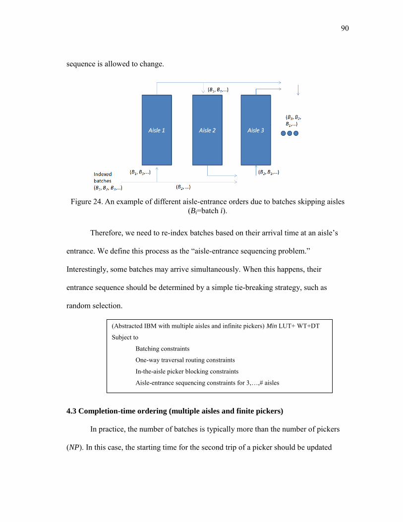
90
sequence is allowed to change.
Figure 24. An example of different aisle-entrance orders due to batches skipping aisles
(Bi=batch i).
Therefore, we need to re-index batches based on their arrival time at an aisle’s
entrance. We define this process as the ―aisle-entrance sequencing problem.‖
Interestingly, some batches may arrive simultaneously. When this happens, their
entrance sequence should be determined by a simple tie-breaking strategy, such as
random selection.
4.3 Completion-time ordering (multiple aisles and finite pickers)
In practice, the number of batches is typically more than the number of pickers
(NP). In this case, the starting time for the second trip of a picker should be updated
(Abstracted IBM with multiple aisles and infinite pickers) Min LUT+ WT+DT
Subject to
Batching constraints
One-way traversal routing constraints
In-the-aisle picker blocking constraints
Aisle-entrance sequencing constraints for 3,…,# aisles
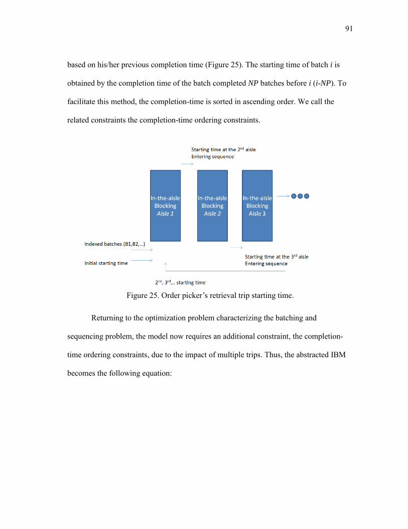
91
based on his/her previous completion time (Figure 25). The starting time of batch i is
obtained by the completion time of the batch completed NP batches before i (i-NP). To
facilitate this method, the completion-time is sorted in ascending order. We call the
related constraints the completion-time ordering constraints.
Figure 25. Order picker’s retrieval trip starting time.
Returning to the optimization problem characterizing the batching and
sequencing problem, the model now requires an additional constraint, the completion-
time ordering constraints, due to the impact of multiple trips. Thus, the abstracted IBM
becomes the following equation:

92
Herein, the updates of the aisle-entrance sequencing, the in-the-aisle picker
blocking, and the completion-time ordering are included in ascending order of time, i.e.,
a first event is processed first. Below, we give two solutions: an MIP formulation and a
next-event advance approach.
5. AN EXACT MIXED-INTEGER PROGRAMMING (MIP) FORMULATION
In this section, we formulate the IBM as a mixed-integer program. We focus on a
general formulation in this section, while the executable MIP formulation is shown in
Appendix C.
5.1 Parameters and decision variables
We consider the general multiple aisle OPS layout as shown in Figure 26. The
OPS has an even number of aisles to allow pickers to traverse the entire picking area
without requiring a u-turn or back-tracking. The pick faces are numbered 0 to Fa+1 at
every aisle. Pick faces 0 and Fa+1 represent the entrance and the exit of an aisle,
respectively. In odd aisles, the entrance is located at the front cross aisle, and for even
aisles entry is from the rear cross aisle. It takes time AE to travel from the entrance to the
first pick face or from the last pick face to an exit. The travel time between neighboring
pick faces is PF. The walk time from 0 to Fa+1 is equal to PF*(|Fa|-1)+2*(AE+PF/2) =
(Abstracted IBM with multiple aisles and finite pickers) Min LUT+ WT+DT
Subject to
Batching constraints
One-way traversal routing constraints
In-the-aisle picker blocking constraints
Aisle-entrance sequencing constraints for 3,…,# aisles
Completion-time ordering constraints for all batches

93
AH when an aisle is passed through. The cross time between two parallel aisles is AW.
The L/U station is located in the front of the leftmost aisle.
Figure 26. An OPS layout.
NP pickers work in the OPS, where NP is assumed to be smaller than the number
of batches. The number of batches is not given, although the number of batches must be
smaller than the number of orders. Two batch picking strategies—pick-then-sort and
sort-while-pick—are considered; the choice of strategy impacts cart capacity. A picker
who completes a trip is reassigned to the next available batch and all pickers are
available initially.
Several decision variables associated with the IBM procedure must be defined:
basically, orders are assigned to batches and to a release sequence through batching
variables; each order includes multiple items; and each item is stored in only one pick
face. Xob is set to 1 when order o is assigned to batch b. The batch sequence at the third
and later aisles is defined through variables ( aijY ). For all a = 3,…,|A|, a
ijY is set to 1
when batch j is released in the ith position of the sequence. The starting time for batches

94
picked on a picker’s second or later trip (STi) can be captured using ordering variables
(Zij) of the completion-time (CTi). Similarly, Zij is set to 1 when batch j is completed in
the ith position of the sequence.
The routing is expressed by the aisle-visiting incident vector. Initially, the vector
for order o at aisle a is given as OAVoa (this vector can be obtained from items in an
order). OAVoa is set to 1 if any item in an order o is stored in aisle a. The route of a batch
is determined by (BAba). If batch b has at least one pick in aisle a, BAba is set to 1. While
evaluating picker blocking, aiAV expresses whether the ith released batch enters in aisle a.
Additional details follow.
Indices and parameters
fF, = the set of pick faces, its index, FFf ,,1 , 0=L/U station or entrance kaA ,, = the set of aisles, and its indices AAka ,,1, aF = the set of pick faces in aisle aaa FAFFFa ,,,1,
jibB ,,, = the set of for the batches, and its indices ,,, bBjib stands for the initial batch number
oO, = the set of orders, and its index Oo
oaOAV = 1 if order o passes through aisle a (order o has at least one pick in aisle a) 0 otherwise
ofOP = the number of picks of order o and pick face f bST = the starting time of thb batch
PTPF, = the walk time to pass one pick face, the pick time to pick an item
NP = the number of pickers
AEAWAH ,,
= the time to pass through an aisle, the width between two aisles, aisle enter/exit
time

95
UTLT,
= the loading time, the unloading time = the time required for the transition between two batches in a pick face
afL ,1 = the leaving time at the previous history
Decision variables
obX = 1 if order o is assigned to batch b (i.e. b is the release sequence at aisle 1) 0 otherwise
aijY = 1 if batch j enters aisle a at the ith order, ||, . ..,3 Aa
0 otherwise
ijZ = 1 if batch j returns to the unloading station at the ith order 0 otherwise
bBV = 1 if batch b is valid 0 otherwise
baBA = 1 if batch b has at least one pick in aisle a 0 otherwise
aiAV
= 1 if the ith batch has at least one pick in aisle a
0 otherwise
NBV
= the number of valid batches
baBAC = the completion time of batch b up to aisle a
bNBA = the number of pairs of aisles visited to retrieve batch b
bRBA = the right most aisle visited while retrieving batch b
bfBP = the picking time of the ith batch at pick face
a
ifa
if CPP ,
= the pick time of the ith batch at pick face f in aisle a, and its cumulative pick time a
ifaif CDD ,
= the time delayed of the ith batch at pick face f in aisle a, and its cumulative
time delayed
aifL
= the leaving time of the ith batch at pick face f in aisle a
aifCW
= the cumulative walk time of the ith batch to pick face f in aisle a
iCT = the completion time of the batch which has finished at the ith order
baba INTINT 2,1
= non-negative integer variables

96
5.2 Objective cost
The goal is to minimize loading/unloading time (LUT) + total walk time (WT) +
total time delayed (DT) (6.1). LUT is proportional to the number of valid batches times
the unit loading/unloading time. The travel time of a batch is the sum of the vertical
travel times (= 2*NBAb*AH) and the horizontal travel times (= 2*RBAb*AW). WT is the
sums of the travel times of all batches. DT is obtained by summing the cumulative delay
at each aisle of all batches.
Min
Aa N BVb
a
FiN BVb
bb CDAWRBAAHNBANBVUTLT a
,,1,,1
22
(6.1)
5.3 Indexed batching constraints
The basic function of the given algorithm is to partition orders into batches. The
actual decision includes the number-of-batches variable (NBV), batching variables (Xob),
and batch validity (BVb). An order cannot be separated (6.2), and a batch should not
exceed the capacity (6.3). When partitioning the orders, NBV should be determined
simultaneously. The maximum number of batches is equal to the number of orders. We
define a binary variable (BVb) to represent the validity of a batch. BVb is obtained from
an OR operation among inclusion flags of orders in batch b (6.4). To avoid alternative
identical solutions regarding batching, we set one additional comparison constraint such
that lower-numbered batches are assigned first (6.5). Constraints (6.6) calculate the
number of valid batches. From the batching information (Xob), the pick time vector of
batches is obtained (6.7).
,1Bb
ob X O, o (6.2)
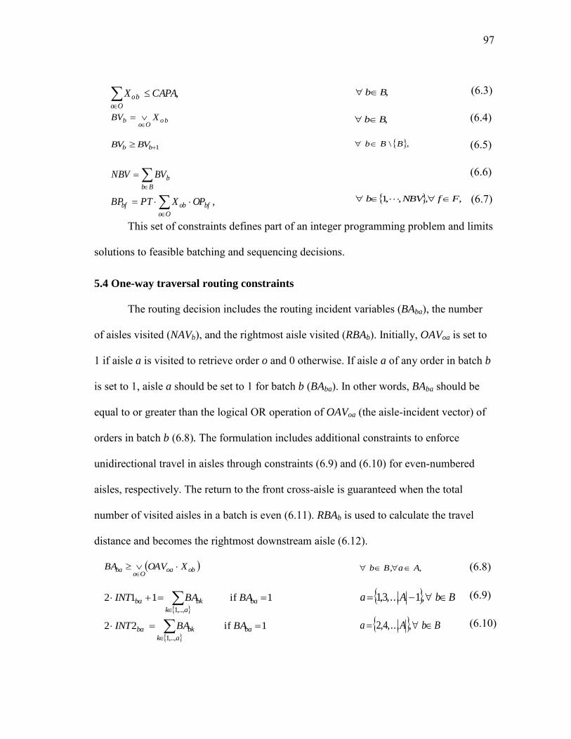
97
,CAPA XOo
ob
B, b (6.3)
o bOo
b XBV
B, b (6.4)
1 bb BVBV
,BB b \ (6.5)
Bb
bBVNBV (6.6)
,
Oo
bfobbf OPXPTBP
F, f,NBV b ,,1 (6.7)
This set of constraints defines part of an integer programming problem and limits
solutions to feasible batching and sequencing decisions.
5.4 One-way traversal routing constraints
The routing decision includes the routing incident variables (BAba), the number
of aisles visited (NAVb), and the rightmost aisle visited (RBAb). Initially, OAVoa is set to
1 if aisle a is visited to retrieve order o and 0 otherwise. If aisle a of any order in batch b
is set to 1, aisle a should be set to 1 for batch b (BAba). In other words, BAba should be
equal to or greater than the logical OR operation of OAVoa (the aisle-incident vector) of
orders in batch b (6.8). The formulation includes additional constraints to enforce
unidirectional travel in aisles through constraints (6.9) and (6.10) for even-numbered
aisles, respectively. The return to the front cross-aisle is guaranteed when the total
number of visited aisles in a batch is even (6.11). RBAb is used to calculate the travel
distance and becomes the rightmost downstream aisle (6.12).
oboaOo
ba XOAVBA
,AaB, b (6.8)
1 if 112,..,1
ba
ak
bkba BABAINT
B bAa ,1,..,3,1 (6.9)
1 if 22,..,1
ba
ak
bkba BABAINT
B bAa ,,..,4,2 (6.10)

98
,2
Aa
bab BANBA B, b (6.11)
,baAa
b BAaMAXRBA
B, b (6.12)
5.5 In-the-aisle picker blocking constraints
In-the-aisle picker blocking constraints evaluate the blocking delay by the
information composed of batches, the start-time of pickers (STi), the aisle-completion
time of batch b (BACba), and the trip-completion time of ith batch (CTi). The calculation
requires the introduction of several intermediate variables: aifCP , a
ifCW , and aifCD stand
for the cumulative pick time, the cumulative walk time, and the cumulative delay time
before leaving pick face f in aisle a of batch b.
aifCW is the cumulative walk time when the picker picking batch i reaches pick
face f in aisle a. The starting time is obtained from STi, CTi and BACba. Constraints (Eq.
5-13) update aifCW at aisle entrances and pick faces. At the loading station (aisle-
entrance 1), aifCW is determined using the pickers’ available time (STi) when the release
sequence is smaller than the number of pickers, otherwise, using the completion time of
the previous trip (CTi). The starting time of batch NP+1 is the completion time of the
first completed batch because the picker responsible for the first completed batch will be
assigned to pick the NP+1st batch. At other aisle-entrances, aifCW is updated by the
previous aisle completion time (BACba) plus aisle crossing time (AW). Otherwise, aifCW
is determined from the previous aifCW 1 when ith batch uses aisle a, i.e., a
iAV = 1.

99
otherwise
1 and 0 if
1 and 0, , if
1 and 0, , if
1,
1
afi
ai
Bj
j,aa
ij
NPi
i
aif
CWAVWT
afAWBACY
afNPiCTLT
afNPiSTLT
CW
A,aF f
,NBV i
a
,0
,,1
(6.13)
The delay time is expressed as the gap between the planned leaving time and the
actual leaving time from a pick face or aisle entrance. An intermediate variable, leaving
time ( aifL ), is introduced to simplify the calculation. This intermediate variable helps to
establish the delay time as a function of the picker’s leaving time and the pick face
available time. Cases 1 through 3 below concern batch i passing through aisle a. In case
4, batch i skips aisle a.
Case-1) When pick face f is not the last pick face in an aisle. Figure 27
illustrates a timeline of a picker blocking situation in a pick face that is not the final pick
face. A picker retrieving batch i leaves pick face f of aisle a at time aifL = a
ifCP + aifCW +
aifCD . Herein, a
iCW 0 stands for the arrival time at the aisle entrance. When the picker
departs pick face f, pick face f is accessible by another picker after transition time (γ).
When pick face f is already occupied, the picker must wait until pick face f is released.
We describe blocking time as the gap between the pick face ready time ( afiL ,1 + γ) and
the planned-arrival time of the trailing picker ( aifCP + a
ifCW + aifCD 1 +PF). At pick face f, a
trailing picker can depart pick face f at aifCP + a
ifCW + aifCD 1 . If the next pick face f+1 is
available without any picker blocking, the picker can arrive at aifCP + a
ifCW + aifCD 1 +PF,
where PF is the walk time between two neighboring pick faces. However, if the next

100
pick face f+1 is not available ( afiL 1,1 + γ > a
ifCP + aifCW + a
ifCD 1 +PF), the picker should
stay at the current pick face ( aifD = a
fiL 1,1 + γ -( aifCP + a
ifCW + aifCD 1 +PF) ), where a
fiL 1,1
is the departure time at the next pick face f+1 of the previous batch i-1. The leaving time,
aifL , is updated to a
ifCP + aifCW + a
ifCD 1 + aifD = a
ifCP + aifCW + a
ifCD , recursively.
Figure 27. Delay time for batch b at pick face f when a picker is blocked.
Case-2) When pick face f is an aisle entrance. When multiple order pickers
arrive together at an aisle entrance, or a picker intentionally waits at the aisle entrance
(to improve downstream blocking), a waiting delay occurs. This delay is allowed at pick
face 0a. Since there is no picking time and no previous delay, if a delay occurs then aiD 0
becomes aiL 1,1 + γ -( a
iCW 0 +AE).
Case-3) When pick face f is the last pick face, |Fa|. At the last pick face of an
aisle, the calculation is unnecessary, because the picker exits an aisle. Thus, we do not
consider picker blocking.
Case-4) When aisle a is skipped. While retrieving a batch, the picker passes
through some aisles and skips others. When a batch skips an aisle, the batch does not

101
need to be used in calculating delay times in the skipped aisle. We update the leaving
time of the batch skipping an aisle ( aifL ) using the leaving time of the previous batch
( afiL ,1 ). To detect if an aisle is being skipped, we use the routing information a
iAV ,
which is a binary variable denoting the usage of aisle a by batch b. The detail is
discussed in Section 5.6.
Constraints (6.14) update the cumulative pick time. Constraints (6.15) calculate
the cumulative delay time. Constraints (6.16) and (6.17) calculate the time delayed ( aifD )
and the leaving time ( aifL ) at pick face f with aisle-incidence vector ( a
iAV ). Constraints
(6.16) implement the delay calculation discussed in the four cases above. Constraints
(6.17) update the leaving time. At an aisle entrance (f = 0), aifL is determined by a
ifCW +
aifCD since there is no pick operation. At a pick face (f>0), a
ifL is assigned with aifCP +
aifCW + a
ifCD if batch i passes through aisle a. When batch i skips aisle a, aifL is assigned
to be equal to afiL ,1 .
,1,afi
aif
aif CPPCP
A,aF f
,NBV i
a
,
,,1
(6.14)
, 001,ai
ai
afi
aif
aif DCDCDDCD
A,aF f
,NBV i
a
,0
,,1
(6.15)
otherwise0
},0{\
and 1 if
0,
0 if0,
1,
1,1
1,1
aa
ai
afi
aif
aif
afi
aif
ai
aif
FFf
AV
PFCD
CWCPLMax
fAECWLMax
D
A,aF f
,NBV i
a
,0
,,1
(6.16)

102
otherwise,1
, 0 and 1 if
0 if
afi
faiififif
ifif
aif
L
fAVCDCWCP
f CDCW
L
A,aF f
,NBV i
a
,0
,,1
(6.17)
5.6 Aisle-entrance sequencing constraints
We establish the release sequence at aisle a in {3,…,|A|} as aijY . The index i
defines a sequence and batch j is released as the ith batch in a sequence when aijY = 1.
Thus, only one batch can be assigned to each sequence position (6.18). Batch j is
assigned to only one sequence position (6.19). Constraints (6.23) establish that the first
completed batch at the previous aisle enters the current aisle first.
As the release sequence is determined, the related variables are assigned. The
pick time vector of batch i at pick face f in aisle a is updated with batch j’s pick time
(6.20). Additionally, the release sequence in each aisle updates the route information of
ith batch ( a
iAV ) (6.21) and the batch completion time in aisle (BAC) using aijY (batch j is
released at ith time in aisle a) (6.22).
1
..,1
NBVj
aijY
,Aa
,NBV i
,,3
,,1
(6.18)
1
..,1
NBVi
aijY
,Aa
,NBV i
,,3
,,1
(6.19)
2,1 if
2,1 if
..,1,
aBPY
aBP
P
NBVjfFaj
aij
ifa
ifa
A,aF f
,NBV i
a
,
,,1
(6.20)
2,1 if
2,1 if
..,1
aBAY
aBAAV
NBVjja
aij
iaa
i
A,a,NBV i ,,1 (6.21)

103
1 and 1 if
1 and 0 if
1 and 1 if
1 and 0 if
..,1
1
1
aBA
aBA
aBA
aBA
AELY
AWBAC
AE L
CW
BAC
b a
b a
b a
b a
NBVi
a
Fi
aib
b ,a -
a
Fb
b
b a
a
a
A,a,NBV i ,,1 (6.22)
j
aja
jij
aja
ij BACYBACY 1,,11,
,Aa
,NBV i
,,3
,,1
(6.23)
5.7 Completion-time ordering constraints
The completion time of the ith batch (CTi) is updated based on the completion
time ordering variables of batches (Zij) and the completion time of the batch at the last
aisle. Zij captures the completed batches such that batch j is the ith batch completed
(6.24), (6.25). CTi shows the completion time of the ith completed batch (the time when
it returns to the unloading station) (6.26), where completion time = exit time at the last
effective aisle + the return time to the L/U station + unloading time. Constraint (6.27)
assures order completion times and the sequences are consistent.
1
..,1
NBVj
ijZ
(a completion sequence must include one batch)
,NBV i ..,1 (6.24)
1
..,1
NBVi
ijZ
(a batch should be assigned to one completion
sequence)
,NBV j ..,1 (6.25)
UTZAWRBABACCTNBVj
ijjRBAji j
..,1,
,NBV i ..,1 (6.26)
1 ii CTCT
,NBV i 1..,1 (6.27)
The final executable MIP formulation is summarized in Appendix C.
5.8 Validation
From the traditional batching and scheduling models, the requirements necessary
to define valid batches and sequences that are sufficiently flexible are defined through
the following set of assumptions. Requirements 1 through 4 maintain the integrity of the
104
order, enforce the capacity of the cart, ensure that routes begin and end at the L/U station,
and allow one-way travel only within aisles. While travelling in an aisle, two pickers
cannot occupy a pick face at the same time and a picker cannot pass another picker in an
aisle (outlined in requirements 5 and 6). When pickers move between aisles, they enter
the next aisle they plan to traverse in a first-come, first-served (FCFS) priority ordering:
Requirement 1 (No split of an order and all order fulfillments). Every order is
included in exactly one batch.
Requirement 2 (Capacity). The number of items in a batch is less than or equal
to the maximum batch size.
Requirement 3 (Complete route). A route must start at and return to the L/U
station.
Requirement 4 (One-way directionality). Each aisle has its own moving
direction.
Requirement 5 (A single picker at a pick face). Only one picker can occupy a
pick face.
Requirement 6 (No-passing in an aisle). Self-explanatory.
Requirement 7 (FCFS at aisle entrance and LU station). The first picker to
arrive starts first at every aisle and LU station.
Requirement 1 is enforced by (6.2) and requirement 2 is enforced by (6.3).
Requirements 3 and 4 can be guaranteed when the constraints in (6.9), (6.10), and (6.11)
are satisfied. (6.16) restricts a picker from entering a pick location occupied by the
former picker; therefore, requirement 5 is enforced. Moreover, the delay time must be

105
greater than or equal to 0. Thus, a trailing picker cannot pass the former picker
(Requirement 6). (6.13) enforces the FCFS sequencing at the LU station and at the
beginning of each aisle (Requirement 7).
6. A SIMULATED ANNEALING (SA) ALGORITHM
Scalability is a major problem in order picking. The model above combines two
NP-hard problems: the order batching problem and the sequencing problem. To handle
large-scale instances, a simulated annealing heuristic procedure is used.
6.1 Simulated annealing procedure
Simulated annealing is widely used in sequencing problems and order batching
problems. We employ an algorithm described in Pinedo (1995), which is illustrated in
Figure 28. For a batching situation, an indexed batching solution is given as BS1 and its
total retrieval time as Obj(BS1). The major characteristic is to accept a worse solution
(BS) while progressively searching for a better candidate solution of solution BSi with
probability P(BSi,BS) = e^( (Obj(BSi)-Obj(BS)/ βi ), where βi is referred to as the cooling
parameter or temperature. To update the cooling parameter (βi), we use a simple function
ai where 0<a<1, a ∈ R (see Pinedo (1995) in detail). Thus, the probability to accept an
incorrect solution gradually decreases as iteration i cumulatively updates the cooling
parameter (βi) using a, i.e., βi= a*βi-1 where i>1 and 0<a<1. To generate an initial
solution (BS1), a large-scale order batching algorithm, RBP see Chapter V, is used which
produces a near-optimal solution when the objective is to minimize the total retrieval
distance. Imax is the maximum number of iterations. T is the updated temperature. Section
7.2.2 discusses how to develop a neighboring solution.

106
Figure 28. A simulated annealing algorithm.
6.2 Picker blocking estimation (Obj(B))
Obj(B) quantifies the blocking time using the mechanism discussed in the
previous section. Figure 29 describes the main procedure. In-the-aisle picker blocking
follows the mechanism shown in Figure 27. We assume that there are NP pickers. p is
index of pickers. Statusp represents the current status of picker p, which includes a batch
index when picker p has an assigned batch, IDLE when the picker is ready for picking or
has no assigned batch, and OFF-DUTY when the last trip has been completed.
Step1. Set i = 1 and T = a.
Initialization
Obtain an initial feasible solution, BS1
Set Imax
Set the best solution BS* = BS1
Step 2. Generate a new batch solution BS from BSi, i.e. BS is the neighboring solution of BSi.
If Obj(BS*)<Obj(BS)<Obj(BSi), set BSi+1 = BS;
Else If Obj(BS)<Obj(BS*), set BS*= BSi+1 = BS;
Else if Obj(BS)> Obj(BSi), set BSn+1 = BS with a probability of e(( Obj(BSi)-Obj(BS) )/T);
Otherwise, BSi+1 = BSi
Step 3. Increase i = i+ 1.
Update the temperature T = T * a.
If i = Imax, then STOP; otherwise, go to Step 2.

107
Figure 29. A picker blocking computation procedure.
7. IMPLEMENTATION AND COMPUTATIONAL RESULTS
This section summarizes the computational implementation and discusses
insights from the results. The experiments analyze the impacts on walk time and delay
time by the proposed integrated batch creation and sequencing framework compared to
other order batching and release approaches. Different order picking strategies and
Step1. Set LUTp, WTp, DTp, PTp = 0.0, and Statusp = IDLE for all pickers ( p= 1,…,NP)
b= 1
Step 2. Select picker p of not OFF-DUTY and smallest LUTp+WTp+DTp+PTp. If tie, randomly choose
if no picker p, go to Step3
Switch (Statusp)
Case picker p has an assigned batch
If not the last visiting aisle // aisle-entrance ordering
In-the-aisle picker blocking on the assigned aisle
Update WTp, DTp, PTp // picks, walks, delay at the aisle
Statusp = Next aisle
Else the last visiting aisle // completion-time ordering
In-the-aisle picker blocking on the assigned aisle
Update LUTp,WTp, DTp, PTp // picks, walks, delay at the aisle
// walks to the L/U station, unloading
Statusp = IDLE
Case picker p has no assigned batch
If b≤ |B|
Assign the next batch // aisle-entrance ordering
Update LUTp,WTp // loading, walks to the first visiting aisle
Statuspk = Batch b
B = b+1
else
Statusp = OFF-DUTY
Step 3. Finish. Return sum of LUTp,WTp, DTp, and PTp
108
pick:walk time ratios are considered to explore the robustness of the proposed
framework. Sensitivity tests are conducted over various order picking environments to
observe the trends in throughput improvement and the computational performance of the
proposed framework.
The MIP formulation is implemented using ILOG CPLEX Callable Library C
API 11.0.4. The simulated annealing algorithm is programmed using C language as are
the data-set generator and the simulation module. The executable files run on Windows
Vista (Xeon 2.66 Ghz CPU, 24 GB memory, 32 bit implementation). For the MIP
algorithm, we disable both the branch-and-cut option and the heuristic search option to
evaluate the exact computational time. To validate the batching results, a discrete-event
simulation method (Law and Kelton, 2000) is used, where the simulation clock is
advanced in the ―next-event time advance‖ approach. Three throughput performance
measurements are reported: the average walk time plus delay time per order (WT+DT),
the average retrieval time per order (RT), and the completion time (CT). The objective is
the minimization of RT.
7.1 Exact approach
We implement the MIP solution described in Appendix C.1 directly and obtain
the exact solution. The exact approach can manage only small problem sizes, which do
not account for real-world problems. However, this approach allows us to test the
impacts of the combined batching and sequencing problem and its computational
improvement when an indexed batching model has been employed.
The profiles in Table 3 are used to generate data. For every parameter setting, we

109
run 20 instances. The item locations are generated according to the class-based storage
policy with A:B:C ratio of 70:20:10 for first aisle: second aisle: remaining aisles,
respectively. The term ―interval‖ represents the inter-departure time between two pickers.
Below, we also test the ―pick-then-sort‖ method where CAPA determines a batch size.
Then, (6.3) is replaced with CAPA XOS
Oo
obo
, where OSo represents the order size.
Table 3. Default order picking and OPS profiles
We consider three different batching and release scenarios. B-then-R generates
batches to minimize the total travel distance and releases batches randomly. B-then-S
generates batches to minimize the total travel distance and sequences the batches to
minimize the total delay time. BSP and IBM consider the release sequence while
partitioning orders into batches. BSP does not use the indexed batching method, but
rather combines the batching problem and the sequencing problem in a single model.
Table 4 illustrates the computational results. The table includes columns LT
(loading and unload time), WT (walk time), DT (time blocked), PT (pick time), RT
(retrieval time), CT (completion time), CPU (average run time in seconds), CPUmax
(longest run time), and CPUmin (shortest run time). We note three important
observations. First, the combined batching and sequencing approach dominates the other
approaches. The BSP and IBM approaches show, on average, 13.2% retrieval time
reduction compared to the B-then-R approach, whereas the B-then-S approach improves
Order picking operation profile OPS profile Order profile Picker profile Strategy Capacity Pick time L/U #aisle #pick faces Width #orders Order size Interval #pickers Speed
Sort-while-pick 4 orders 5 10 4 10 2 16 2 1 4 1
Pick-then-sort 10 items 5 10 4 10 2 16 2 1 4 1

110
the throughput on average about 8.0% with the same storage strategy. However, the CT
lengthens (inevitable, since we use a small problem size). This issue will be revisited in
the next section with a large problem size. Second, IBM dominates the BSP method
when comparing the computational time. Third, despite the small problem size and an
optimal IBM approach, we do not find a no-blocking result in an optimal model.
Table 4. Experimental results of the exact approach
7.2 Simulated annealing approach for large-size applications
7.2.1 A mail order company example
A mail order company warehouse operation is analyzed as an example of a large-
scale order picking profile as described in Petersen (2000). The order picking
environment, e.g., the number of aisles, the pick:walk time ratio, the number of pickers,
the number of orders, etc., also derives from Petersen (2000); however, Petersen does
not vary the pick to walk time ratios. To determine the ratios, Gue et al. (2006)’s
recommendation of a ratio of 20:1 or smaller is used. Most academic studies have used
5:1~10:1 (Gong and De Koster, 2008; Gue et al., 2006; Petersen, 2000). Thus, values on
the range 2:1~20:1 were used in experimentation. Reported below are the two most
commonly used ratios of 5:1 and 10:1. For every parameter setting, we test 20 instances.
Strategies Scenarios LT WT DT PT RT CT CPU CPUmin CPUmax
Sort- B-then-R 20.0 33.9 16.1 37.9 107.9 130.1 0.29 0.23 0.47
while- B-then-S 20.0 33.9 8.0 37.9 99.8 109.4 0.27 0.22 0.34
pick BSP 20.0 34.1 1.6 37.9 93.6 122.2 1883.23 128.53 8507.01
IBM 20.0 34.1 1.6 37.9 93.6 121.2 142.04 35.72 632.30
Pick- B-then-R 20.0 35.1 16.6 44.3 115.9 141.6 0.26 0.19 0.41
then- B-then-S 20.0 35.1 6.8 44.3 106.1 111.8 15.26 68.00 119.20
sort BSP 20.0 35.1 1.2 44.3 100.5 125.1 512.36 63.10 2679.03
IBM 20.0 35.1 1.2 44.3 100.5 125.8 63.38 13.82 180.72

111
The picking environment is summarized in Table 5.
Table 5. Configuration of an OPS (modified from Petersen example (Petersen, 2000))
Profiles Values Pick:walk time ratio Number of aisles Walk time Number of pick faces / aisle Pick time Number of pickers Cycle length Number of orders (per cycle) Loading / Unloading time Order size SKU P/D location ABC class rule Capacity Order picking strategy
2:1, 5:1, 10:1 , 20:1 10, 20, 30 PF = 1 seconds/pick face, AE = 0.5 second, AW = 2 seconds 20 pick faces 2, 5, 10, 20 seconds 8, 16, 24 (starting interval = 1.0 seconds) 1 hour 360, 720, 1080, 1440 Each 60 seconds 2.02 ( p(1) = 0.5/0.95, p(n)=( 1/2*(n-1)-1/2*n )/(0.95) when n=2,…,10,
and p(n) = 0 otherwise.), Unif(1,3), Uniform(3,9), Uniform(5,15) 1 Center of the leftmost aisle Demand portion and aisle size 70%:20%:10% = 2:2:6, 50:30:20, Random 10 orders, 30 items Sort-while-pick, pick-then-sort
In discussing the performance of the algorithms, we use the following notation
throughout the remainder of this section.
WT+DT: the average total walk time (WT) plus total time blocked (DT) per order
RT: the average retrieval time per order
CT: the completion time of the last completed batch
LB: the linear relaxation model of RBP
IBMsa: the indexed batching procedure with simulation annealing, where this study
uses a = 0.8 after a preliminary experiment
Obj: the objective value of an algorithm
Red : reduction ratio by an algorithm compared to the RBP + random release
method expressed as a percentage ( = (an objective function value of the RBP
+ random release method – the objective function value of an algorithm)/( an
objective function value of the RBP + random release method ) %)
LU gap: gap between an objective function value and the LB objective function

112
value expressed as a percentage ( = (an objective function value – the LB
objective function value)/(the LB objective function value) %)
CPU: the run-time in seconds
7.2.2 Neighborhood search
The method for defining a neighborhood in a simulated annealing procedure is
critical to effective implementation (Pinedo, 1995). Four methods that can be used to
define the neighborhood in which to search were investigated. In the first method, NB1,
a general two-exchange method is employed where a pair of orders is exchanged. We
randomly pick two batches (b1, b2) and two orders (o1, o2) from each batch. The new
neighborhood becomes b1 with o2 and b2 with o1. Next, we develop three more
neighborhood methods. The method NB2 switches b1 with b2, changing the sequence of
batches to be picked. The orders in each batch do not change. NB3 and NB4 set an
acceptance condition on NB1. In NB3, b2 is selected among batches having the same
route. In NB4, the new neighborhood must keep the current travel distance.
NB1. batches and orders change
NB2. batches change sequence
NB3. batches and orders change if two batches have the same route
NB4. batches and orders change if new batches have at most the same distance
Alternative neighborhood definitions are compared in Table 6 relative to
different pick:walk time ratios. NB1 and NB4 are dominant. Specifically, when the
congestion is light, NB4 is slightly better than NB1. Since the initial solution guarantees
a near-optimal travel distance for the picker, the approach to search a neighbor in order
to reduce the blocking time is effective. In contrast, when heavy congestion exists, NB1
identifies better solutions. NB1 searches a much larger solution space than NB4, because

113
NB1 considers both the distance reduction and the delay reduction.
Table 6. Comparison of neighborhood rules in simulated annealing approach
Rules 5:1 10:1 WT+DT CPU WT+DT CPU
NB1 7.79 70.46 8.86 84.42
NB2 8.43 323.87 11.17 482.78
NB3 7.87 54.55 9.74 53.14
NB4 7.62 73.67 9.21 77.68
7.2.3 Comparison to available algorithms
Table 7 and Figure 30 compare the IBMsa method to other available batching
methods. The FCFS method groups orders into batches sequentially, and releases the
batches as they arrive. The seed algorithm is one of the most common batching methods.
The best seed algorithm in De Koster et al. (1999) is reported below. The CW II
approach, a variation of the Clarke and Wright algorithm (1964) appearing in De Koster
et al. (1999), is also considered. The table includes the performance of RBP. The LP
relaxation described in Chapter IV is used to obtain a lower bound (LB). Seed, CW II,
and RBP minimize only the travel distance and do not handle the release sequence. Thus,
the grouped batches are released in a FCFS manner.
Table 7 and Figure 30 (a) show how IBM dominates the other methods based on
the WT+DT criteria. The run time is less than 2 minutes. Specifically, the proposed
IBM achieves a 2.5 to 18% reduction in the total retrieval time compared to the near-
optimal distance-only approach, RBP, as depicted in Figure 30 (b).

114
Table 7. Comparison of WT+DT per order 2:1 5:1 10:1 20:1 WT+DT CPU WT+DT CPU WT+DT CPU WT+DT CPU FCFS + Random release
17.69 20.25 25.39 36.84
Seed algorithm + Random release
11.14 0.03 15.65 0.03 24.00 0.03 42.04 0.03
CW (II) + Random release
8.69 136.93 11.44 135.70 16.92 135.77 28.90 133.78
RBP + Random release
7.65 46.80 9.91 49.03 14.50 48.53 24.51 48.74
IBMsa 7.04 67.34 7.79 81.92 8.86 90.76 10.78 101.32
(a) (b)
Figure 30. Algorithm comparison with different throughput measurements: (a) WT+DT per order; and (b) Walk time+delay time % in the total retrieval time.
7.2.4 Comparison across the number of orders
Table 8 summarizes the results across the number of orders over two batching
strategies. Compared to the best distance-based algorithm (RBP), IBMsa experiences
approximately 5 % to 14.0% reduction of the total retrieval time. The solution from
optimizing the retrieval time also results in 4% to 12% reduction of the completion time
(CT). When the pick:walk time ratio is small, the percentage reduction in retrieval time
decreases and the percentage gap to the lower bound is small. Both the sort-while-pick
strategy and the pick-then-sort strategy show a stable improvement of the total retrieval
time. When the problem size is small, IBMsa performs better, because the search space is
relatively smaller.

115
Table 8. Variation of the number of orders over two batching strategies
7.2.5 Other order picking profiles
Note that order picking environments can be more diverse. Table 9 summarizes
the results of additional experiments varying the number of aisles, storage policy,
number of pickers, and order size. The sort-while-pick strategy is evaluated for the
pick:walk time ratio of 5:1.
Storage policy
The storage profile in Table 9 exhibits an interesting result. When the pick:walk
time ratio = 10:1, the random storage policy performs best under no sequencing control.
After applying the IBM, the class-based approaches perform better based on the total
retrieval time criteria. This finding stresses a critical issue concerning the
interdependence of the storage policy and the order-size pattern and number of pickers.
If the class-based approach is used, the benefits of applying IBM are significant.
The number of pickers
More pickers cause more blocking. The proposed procedure shows an
Pick: Stategy # RBP+Random release LB IBMsa -best
walk orders RT CT
ratio WT WT+DT RT CT RT WT+DT Obj Red% LU gap % Obj Red% LU gap % Rule CPU
5:1 Sort 360 7.08 11.37 33.33 944.28 28.88 8.47 30.42 8.7% 5.3% 870.25 7.8% 32.4% NB1 30.30
while 720 6.72 9.91 31.89 1608.88 28.62 7.79 29.77 6.7% 4.0% 1504.50 6.5% 16.1% NB1 69.00
pick 1080 6.63 9.34 31.39 2305.15 28.61 7.40 29.45 6.2% 2.9% 2170.03 5.9% 11.9% NB4 138.57
1440 6.59 9.24 31.29 3008.38 28.57 7.33 29.38 6.1% 2.9% 2827.03 6.0% 9.6% NB4 159.86
Pick 360 5.92 11.34 29.41 929.15 23.63 8.36 26.44 10.1% 11.9% 875.33 5.8% 62.3% NB1 111.21
then 720 5.69 9.49 27.56 1493.90 23.50 7.25 25.32 8.1% 7.7% 1397.05 6.5% 31.2% NB1 148.65
sort 1080 5.70 8.62 26.78 2088.13 23.61 6.97 25.13 6.2% 6.4% 1957.08 6.3% 22.2% NB1 225.22
1440 5.61 8.25 26.42 2636.83 23.53 6.87 25.04 5.2% 6.4% 2521.55 4.4% 18.6% NB4 298.70
10:1 Sort 360 7.08 16.83 48.74 1371.15 38.84 9.49 41.40 15.1% 6.6% 1220.65 11.0% 38.5% NB1 37.12
while 720 6.72 14.50 46.47 2351.93 38.60 8.86 40.82 12.1% 5.7% 2098.08 10.8% 20.3% NB1 82.05
pick 1080 6.63 13.62 45.72 3362.13 38.66 8.89 40.99 10.3% 6.0% 3027.43 10.0% 15.7% NB1 154.65
1440 6.59 13.51 45.60 4390.95 38.61 9.02 41.11 9.8% 6.5% 3973.35 9.5% 14.1% NB1 180.00
Pick 360 5.92 17.28 45.31 1369.80 33.59 10.25 38.27 15.5% 14.0% 1237.70 9.6% 62.2% NB1 107.51
then 720 5.69 13.86 41.91 2269.18 33.48 8.86 36.91 11.9% 10.2% 1995.40 12.1% 31.8% NB1 148.53
sort 1080 5.70 12.42 40.62 3085.15 33.66 8.53 36.73 9.6% 9.1% 2828.80 8.3% 24.1% NB4 217.20
1440 5.61 11.80 40.01 3958.68 33.58 8.29 36.50 8.8% 8.7% 3631.93 8.3% 19.9% NB4 298.96

116
improvement beyond the other methods investigated. RT reduction and CT reduction are
9.7% and 8.8%, respectively when the pick:walk time ratio = 5:1. With a higher
pick:walk time ratio, more blocking occurs and the IBM algorithm shows greater
benefits on a percentage basis.
The number of aisles in OPS
In larger OPS, pickers ―spread out‖ in a picking area and there is less picker
blocking. Thus, the benefit from IBM diminishes. ―-‖ means that a lower bound solution
could not be obtained because the problem size is too large.
Order size
We test three different order sizes. The IBM algorithm shows a robust benefit
over all values.
Table 9. The experimental results over diverse order picking environments
7.2.6 Side effects in a large-scale application
The control of picker blocking minimizes both the RT per order and the
Pick: RBP + Random release LB IBMsa - Sort-while-picking policy - best
walk Profiles Values RT CT
ratio WT WT+DT RT CT RT WT+DT Obj Red % LU gap% Obj Red % LU gap% Rule CPU
5:1 Default 6.72 9.91 31.89 1608.88 28.62 7.79 29.77 0.07 0.04 1504.50 0.06 0.16 NB1 69.00
Storage 5:3:2 7.69 9.64 31.62 1603.38 29.54 8.35 30.33 0.04 0.03 1532.53 0.04 0.15 NB4 153.76
random 9.24 10.40 32.38 1624.33 31.04 9.68 31.66 0.02 0.02 1595.20 0.02 0.14 NB4 203.89
#pickers 8 6.72 8.16 30.14 2832.10 28.62 6.93 28.91 0.04 0.01 2723.70 0.04 0.06 NB4 28.91
24 6.72 11.87 33.85 1221.53 28.62 8.59 30.57 0.10 0.07 1114.35 0.09 0.28 NB1 87.37
#aisles 20 10.14 11.77 33.77 1712.80 - 10.78 32.78 - - 1664.03 - - NB4 444.29
30 14.07 15.19 37.23 1850.35 - 14.41 36.46 - - 1805.65 - - NB4 654.93
order U(1,3) 6.98 9.34 31.32 1590.30 28.87 7.56 29.53 0.06 0.02 1498.95 0.06 0.15 NB4 83.45
size U(3,9) 11.13 17.30 59.25 2942.38 52.98 12.88 54.83 0.07 0.03 2757.43 0.06 0.15 NB4 478.31
U(5,15) 13.41 22.60 84.64 4194.13 75.34 16.22 78.26 0.08 0.04 3885.93 0.07 0.14 NB4 812.01
10:1 Default 0 6.72 14.50 46.47 2351.93 38.84 8.86 40.82 0.12 0.05 2098.08 0.11 1.38 NB1 82.05
Storage 5:3:2 7.69 12.42 44.38 2269.83 39.52 9.26 41.23 0.07 0.04 2110.55 0.07 0.18 NB4 168.26
random 9.24 12.09 44.05 2258.65 41.02 10.46 42.42 0.04 0.03 2166.98 0.04 0.17 NB4 213.22
#pickers 8 6.72 10.35 42.31 3983.85 38.84 7.24 39.20 0.07 0.01 3703.53 0.07 0.06 NB4 64.74
24 6.72 19.10 51.07 1850.28 38.84 10.61 42.57 0.17 0.10 1546.25 0.16 0.32 NB1 108.56
#aisles 20 10.14 14.28 46.26 2367.10 - 11.79 43.77 - - 2249.88 - - NB4 465.15
30 14.07 17.08 49.11 2454.68 - 15.21 47.24 - - 2360.50 - - NB4 677.16
order U(1,3) 6.98 12.90 44.86 2289.23 38.85 8.29 40.25 0.10 0.04 2042.75 0.11 0.16 NB4 120.33
size U(3,9) 11.13 24.82 96.72 4792.23 82.93 14.82 86.72 0.10 0.05 4360.45 0.09 0.17 NB4 1104.61
U(5,15) 13.41 32.92 144.99 7165.48 125.37 19.26 131.34 0.09 0.05 6513.75 0.09 0.15 NB4 1772.90

117
completion time. Table 10 includes additional analysis regarding the average and the
standard deviation of inter-arrival times between pickers. We collect the inter-arrival
time between pickers at the LU station and the 2nd aisle. With the proposed procedure,
the inter-arrival time becomes smaller and less variable. The smaller variance may
indicate that the pickers are more evenly spaced using the IBM method.
Table 10. Comparison of inter-completion time (the number of orders=2160, Imax=20000)
8. CONCLUSION AND FURTHER STUDIES
This chapter presented: 1) the framework to optimize the order picking operation
in a circumnavigational order picking system, where both travel distance and time
blocked should be assessed; 2) the indexed order batching model (IBM) combining the
order batching problem and the batch sequencing problem; and 3) a simulated annealing
heuristic procedure to allow analysis of realistic problem sizes. The narrow-aisle
structure was exploited in developing the framework, the algorithm, and the procedure.
Experimental results showed that consideration for blocking in an integrated batching
and sequencing approach can have substantial benefits on performance criteria such as
total retrieval time or completion time.
This chapter has taken an initial step towards controlling congestion in a DC
5:1 10:1
Sequence LU station 2nd aisle LU station 2nd aisle
#pickers method RT CT Avg Std Avg Std RT CT Avg Std Avg Std
8 pickers RBP+Rand 29.76 8165.88 36.87 33.71 47.43 47.54 41.86 11494.53 52.07 49.07 66.67 71.61
IBMsa 28.69 7868.70 35.49 28.82 45.63 43.37 38.94 10696.53 48.39 40.63 61.83 64.65
16pickers RBP+Rand 31.09 4376.40 19.24 19.09 24.36 28.43 45.26 6386.68 28.32 29.35 35.56 44.64
IBMsa 29.18 4108.70 18.02 16.90 22.72 26.59 40.59 5688.20 25.09 23.42 31.17 32.20
24pickers RBP+Rand 32.55 3148.18 13.53 14.60 16.87 21.08 48.80 4729.53 20.61 23.10 25.46 33.32
IBMsa 29.95 2883.88 12.32 11.99 15.26 17.33 41.94 4010.88 17.22 16.79 21.21 23.01

118
facility. Specifically, we focused on the narrow-aisle order picking system, which is an
attractive OPS layout due to its cost merit from the standpoint of the DC design. The
proposed order picking operation procedure requires a reevaluation of some previous
research findings. For example, Ruben and Jacobs (1999) recognize the possibility of
productivity loss due to congestion under a class-based storage policy, which tends to
increase pick-density to shorten the travel distance. However, our experimental results
over the variation of the storage policy showed that if appropriate batching and
sequencing procedures, such as IBM, are implemented the congestion in a class-based
policy can be mitigated. IBM can also play a vital role in minimizing or preventing
picker utilization from dropping as the number of pickers increases. According to Gue et
al. (2006), the picker utilization drops as more pickers are staffed in an order picking
system. Thus, it is clear that under IBM some order picking system design rules relevant
to picker blocking should be reconsidered.
We suggest that our research be expanded to consider dynamic controls and to
explicitly account for other idle factors. First, to handle real-world problems, more
dynamic situations should be considered, for example, picking environments that
encounter cart breakdowns, search failures, and order changes. IBM requires new
planning when any of these difficulties are present. Second, while this study only
considers picker blocking, some order picking strategies encounter different idle factors,
such as hand-off delay in bucket brigade systems (Koo, 2009), which is a topic we will
address in the next chapter.

119
CHAPTER VII
ANALYSIS AND CONTROL OF PICKER BLOCKING IN A BUCKET
BRIGADE ORDER PICKING SYSTEM
Bucket brigades is an operation mode for order picking systems, which is
characterized by its self-balancing nature and high pick rates (Bartholdi and Eisenstein,
1996a). However, due to variability and uncertainty of the pick locations within a
particular order or batch, picker blocking can cause productivity losses. Furthermore, the
hand-off operation, which involves transiting partially-picked orders or batches from
upstream pickers to downstream pickers, can result in delays for the downstream pickers.
This chapter examines the significance of picker blocking and hand-off delay in bucket
brigade order picking and identifies the relevant analytical models, highlighting the
issues of blocking and hand-off delay through simulation studies. Our analytical results
identify several conditions for high order picking throughput, such as batch picking,
stable picking performance, and intermediate hand-off. A complete control procedure for
dynamic order picking is provided that mitigates both picker blocking and hand-off
delay. The proposed framework experiences 7 to 12% improvement of utilization across
diverse order picking situations when five pickers pick on average 20 items per tote.
1. INTRODUCTION
1.1 Bucket brigade order picking
A bucket brigade operational policy is attractive because the workload balancing

120
characteristic that allows dynamic reassignment of zones increases productivity with
minimal managerial or planning requirements. In the warehousing industry, the order
picking operation consists of retrieving customer orders from storage. To increase
throughput, multiple orders are often grouped in a batch for more efficient picking
operations.6 The method by which batches are assigned to pickers can have a significant
impact on picking performance. The bucket brigade concept used in general assembly-
line operations can be applied to order picking to achieve valued properties, such as the
self-balancing characteristic and minimum work-in-process (WIP) (Bartholdi and
Eisenstein, 1996a; Bartholdi and Eisenstein, 1996b). In practice, a bucket brigade order
picking strategy is often used with flow-rack shelving (Figure 31) in high throughput
warehouse environments. In this study, the combination of flow-rack shelving and the
bucket brigade strategy discussed in Bartholdi and Eisenstein (1996a) is referred to as a
bucket brigade order picking system (OPS).
Figure 31. A flow-rack OPS (Bartholdi and Eisenstein, 1996a).
The bucket brigade OPS is characterized by limited WIP, high picking
6 We discuss order pickers gathering batches. However, if batching is not used this would imply
one order per batch.

121
throughput, high space utilization, and the self-balancing property (Bartholdi and
Eisenstein, 1996a). However, as pick requirements are random over pick locations,
pickers often encounter blocking when the downstream picker is busy. In addition,
pickers may stand idle when the hand-off process is not synchronized.
In a bucket brigade OPS, multiple pickers help to pick a single batch. Pickers are
sequenced from upstream to downstream, and the sequence is maintained throughout.
Each batch is picked to a tote, and the tote is passed from one picker to the next
traversing the aisle. Pickers collect items at related pick faces in sequence. A picker
picks an item and places it in the tote assigned to a particular batch. The picker then
moves to the next pick face to continue processing the batch if there is no picker at the
next pick face. The upstream picker hands off the current tote upon meeting a
downstream picker who has no assigned tote. The picker most upstream (the first picker)
retrieves a new batch and tote from a loading station and begins picking at the first pick
face. The last picker releases the completed batch to the unloading station. A work area
for a picker is not predetermined and is dynamically resized through the pick-and-pass
process. Thus, this strategy eliminates the need for work zone load balancing, which can
be complicated and difficult (Bartholdi and Eisenstein, 1996a).
1.2 Performance under picker blocking and hand-off delay
A bucket brigade OPS does not allow pickers to pass due to the higher space
utilization (Bartholdi and Eisenstein, 1996a). Not allowing pickers to pass one another
can cause a delay in two ways. First, an upstream picker attempts to move forward to the
next pick face that is occupied by a busy downstream picker as shown in Figure 32 (a).

122
In this situation the upstream picker cannot hand-off the current batch to the downstream
picker because the downstream picker is currently executing a retrieval task. The
upstream picker also cannot pass over the downstream picker, because passing is not
allowed (picker blocking). Second, delay can occur when the downstream picker moves
upstream to take a hand-off from an upstream picker. If the upstream picker is picking
when the downstream picker encounters the upstream picker, the downstream picker
must wait until the upstream picker completes the pick. This is termed hand-off delay as
shown in Figure 32 (b).
(a) (b)
Figure 32. Delay situations in bucket brigade order picking: (a) picker blocking; and (b) hand-off delay.
Performance regarding picker blocking and hand-off delay in bucket brigade
OPS is not well understood. In order to achieve the highest throughput, an individual
order picker’s region of operation within the aisle should stabilize so that the picker can
become familiar with the set of items and their location within the region (Lim and Yang,
2009). In diverse bucket brigade situations researchers (Armbruster and Gel, 2006;
Bartholdi and Eisenstein, 1996b; Bartholdi and Eisenstein, 2005; Bartholdi et al., 2001)
have identified operation rules or conditions that lead to stability. However, picker
blocking and hand-off delay can impact picker utilization (Bartholdi and Eisenstein,

123
1996b) and this issue has received little attention in the literature to date. Only Koo
(2009) investigates the productivity loss due to picker blocking and hand-off delays in a
bucket brigade OPS using simulation under the assumption picker capability is identical.
The throughput loss is 26.1% of the total working time, with 15.6% loss due to picker
blocking and 10.5% loss due to hand-off delay. To our knowledge, there is no analytical
model on picker blocking and hand-off delay in bucket brigade OPS which can help
engineers develop more effective operational strategies.
1.3 Our scope and goals
Order picking throughput is often measured by the ratio of time spent to pick to
time spent at a stop. Gue et al. (2006) introduced the throughput model for a narrow-
aisle order picking system with k pickers. We generalize Gue et al.’s result for a bucket
brigade OPS as described in Equation (7.1). When pickers are blocked with a fraction of
the time, b(k), where 0 ≤ b(k) ≤ 1, and a hand-off takes E[HO], where 0 ≤ E[HO] ≤
maximal pick time at a pick face, the throughput is:
kbHOEnkttptE
ptEkk
wp
1
][/1][
][
(7.1)
where E[pt] stands for the expected number of picks at a stop and n is the number of
pick faces in bucket brigade OPS. The time to pick (tp) represents the average time the
picker is stopped and includes the time spent picking items. The time to walk (tw)
indicates the average time to walk past a pick face (location).
We assume that pickers perform identically, which is persuasive due to
simplicity of order picking, the relatively easy learning curve in order picking, and the
124
use of technology. In our model, walk speed is not instantaneous for both forward and
backward directions. Items in orders are randomly located in n pick faces and the
number of pickers (k) is relatively small compared to n. The time to load and unload
orders at the beginning and end of the aisle is negligible. Importantly, passing is not
allowed in this high density bucket brigade operation.
We develop analytical models for picker blocking and hand-off delays in a
bucket brigade OPS, where no correlation between two delays is assumed. We conduct a
simulation study to clarify the source of delays in diverse situations. The analytical and
simulation models allow for the size of delays to be quantified; however, a primary
purpose of our examination is to assist operational decision-making. A control model
and relevant algorithms are proposed to reduce the delays.
The chapter is organized as follows. Section 2 reviews the relevant order picking
literature and identifies new opportunities. In Section 3, we introduce analytical models
and control methods for picker blocking. Section 4 focuses on an analytical model of
hand-off delay and details the proposed control policy for reducing hand-off delay.
Section 5 describes a simulation study analyzing picker blocking and hand-off delay and
summarizes the experimental results. Section 6 concludes this chapter.
2. LITERATURE REVIEW
Bucket brigade models are typically characterized by work content model
(uniform or exponential), walk speed assumptions (finite or infinite speed in forward and
backward walks), and pickers’ velocity or capability (identical or non-identical). Bucket
brigade was originally proposed for the manufacturing setting, thus descriptions of this

125
work have been adapted for an order picking setting.
2.1 Picker blocking and hand-off delay in bucket brigades
Bartholdi and Eisenstein (1996b) introduce the bucket brigade management
method for manufacturing settings. Their three assumptions are: pickers travel with
instantaneous walk speed (including backward walk speed), a picker’s capability is
distinct and not identical, and workloads are uniformly and randomly distributed. Their
model considers non-identical capability and utilizes the capability difference to reduce
blocking. The highest throughput is obtained when pickers are sequenced with the
slowest picker in the location most upstream and the fastest picker in the location most
downstream. Picker blocking can be minimized when there are large capability
differences among pickers. The authors also suggest that hand-off delay can be reduced
through practice.
Bartholdi and Eisenstein (1996a) present the bucket brigade for order picking and
describe the productivity improvements through a physical implementation. In particular,
the authors emphasize that bucket brigades can achieve both high space utilization and
high picker utilization. However, since higher space utilization makes passing difficult,
they recommend the bucket brigade for high-volume, limited space picking operations
over the more traditional zone picking strategy. Further, the authors suggest another way
to reduce picker blocking is cooperation between neighboring pickers, where a blocked
picker aids a blocking picker with the help of pick-to-light technology. A blocked picker
picks items of a blocking picker, which are identified by pick-to-light.
Bartholdi et al. (2001) develop a general performance model where the work

126
load is not uniform over the pick area. They show that bucket brigades is still
advantageous and self-balancing despite the fact that pick locations are exponentially
distributed. Their assumption states that when walk speed is instantaneous, pickers move
rapidly. Thus, hand-offs of all pickers occur simultanesously and sychronously, and
hand-off delays drop.
Bartholdi and Eisenstein (2005) analyze an assembly-line where the walk speed
is not infinite and the return trip of a picker after handing off his/her workload requires
significant time. Under these assumptions hand-off delay affects productivity. They find
a considerable loss of productivity by walk-back time and hand-off delay; nonetheless,
their practical application demonstrates a stable performance. Specifically, they assume
constant hand-off time to identify the operational stability, but do not evaluate the
productivity loss due to the hand-off operation. They do not observe the impacts of
picker blocking.
Koo (2009) shows that picker blocking and hand-off delay reduce the
productivity of the bucket brigade OPS when pickers have the same capability. The
author assumes that work load is random, pick time is not deterministic, and walk time is
infinite. He constrains each picker’s picking area by defining a downstream boundary
which he shows improves their productivity. Further, upstream pickers are allowed to
leave totes at the boundary location if a downstream picker is not available to take over
the tote. Under this set of assumptions Koo derives a closed form calculation for hand-
off delay as (k-1)*E[pick time]/2.
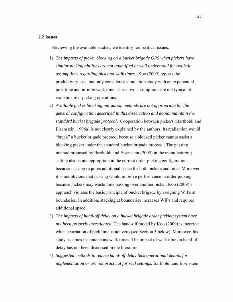
127
2.2 Issues
Reviewing the available studies, we identify four critical issues:
1) The impacts of picker blocking on a bucket brigade OPS when pickers have
similar picking abilities are not quantified or well understood for realistic
assumptions regarding pick and walk times. Koo (2009) reports the
productivity loss, but only considers a simulation study with an exponential
pick time and infinite walk time. These two assumptions are not typical of
realistic order picking operations.
2) Available picker blocking mitigation methods are not appropriate for the
general configuration described in this dissertation and do not maintain the
standard bucket brigade protocol. Cooperation between pickers (Bartholdi and
Eisenstein, 1996a) is not clearly explained by the authors. Its realization would
―break‖ a bucket brigade protocol because a blocked picker cannot assist a
blocking picker under the standard bucket brigade protocol. The passing
method proposed by Bartholdi and Eisenstein (2005) in the manufacturing
setting also is not appropriate in the current order picking configuration
because passing requires additional space for both pickers and totes. Moreover,
it is not obvious that passing would improve performance in order picking
because pickers may waste time passing over another picker. Koo (2009)’s
approach violates the basic principle of bucket brigade by assigning WIPs at
boundaries. In addition, stacking at boundaries increases WIPs and requires
additional space.
3) The impacts of hand-off delay on a bucket brigade order picking system have
not been properly investigated. The hand-off model by Koo (2009) is incorrect
when a variation of pick time is not zero (see Section 5 below). Moreover, his
study assumes instantaneous walk times. The impact of walk time on hand-off
delay has not been discussed in the literature.
4) Suggested methods to reduce hand-off delay lack operational details for
implementation or are not practical for real settings. Bartholdi and Eisenstein

128
(1996a) suggest a smooth hand-off operation; however, there is no description
of the operational implementation. In addition, simultaneous and sychronous
hand-off (Bartholdi et al., 2001) does not apply when both pick time and walk
time are finite.
3. ANALYSIS AND CONTROL OF PICKER BLOCKING
In this section, we develop analytical models of picker blocking and methods to
mitigate picker blocking for bucket brigade OPS. Recognizing that both standard
multiple-aisle rectangular order picking systems and bucket brigade order picking
systems can be characterized using the circular-aisle OPS abstraction, we apply the
blocking control model developed in Chapter V to a bucket brigade OPS under the
assumption of no passing. Finally, we utilize the control model to demonstrate the
reduction that can be achieved.
3.1 Picker blocking in a circular order picking aisle with two pickers
Gue et al. (2006) investigate the effects of picker blocking under a no-passing
policy, considering only single-pick situations. The circular order picking aisle
abstraction is used in developing both analytical models and a simulation study. Table
11, column 1, shows the closed-form expression for percentage of time blocked for two
pick to walk time ratios developed in Gue et al. (2006). Column 2 presents our results in
Chapter V. The analysis is undertaken for a two-picker OPS. Both approaches consider
two extreme cases: 1) walk speed is equal to unit pick time per pick face (pick time:walk
time = 1:1), and 2) walk speed is infinite (pick time:walk time = 1:0). The results in
Table 11 are developed for a rectangular multiple aisle warehouse with cross aisles at the
front and back of the picking area. Pickers take a one-way traversal route and passing is

129
not allowed. At a pick face, a batch includes an item with a probability p. Further, q
denotes 1-p, the probability of no item at a pick face. The models of Gue et al. (2006)
and Chapter V are distinguished by the number of picks per pick location, single vs.
multiple. The multiple-pick model can repeat a pick at the same pick face with
probability p.
Table 11. The percentage of time blocked when two pickers work (p=pick density, n=the number of pick faces)
Pick:walk time
Single-pick (Gue et al., 2006)
Multiple-picks (see Chapter V)
1:0 pnp
p
112
1
pn 12
1
1:1
2211 ppn
pq
12 pn
p
Gue et al. (2006) explain that the batch picking strategy can experience less
picker blocking when the pick density is either very low or very high. Chapter V and
Parikh and Meller (2010) show that the variation in pick density can be as important as
the level of pick density in determining the amount of blocking in a circular-aisle OPS.
One important observation in Chapter V is that batch picking can reduce picker blocking.
3.2 Picker blocking in bucket brigade order picking
Bucket brigade order picking has a special release mechanism of a new batch and
the mechanism impacts the picker blocking model. Thus, first, the release mechanism of
a new batch is explained. Second, picker blocking will be discussed. Note that in this
study we show the equivalence of the picker blocking models of the bucket brigade
order picking and the circular-aisle abstraction under specific situations, instead of a

130
direct development of the picker blocking model of bucket brigade order picking.
Figure 33 describes a series of hand-offs after completion of a batch. k pickers
are sequenced from the loading station to the unloading station in a decreasing sequence
of k,k-1,…, 2,1. When a batch (denote this batch ith batch) is finished by the picker most
downstream (picker 1), a new batch must enter the system. Picker 1 becomes idle and
moves backward to take over the batch of picker 2 who is moving forward with the i+1st
batch. Obviously, the hand-off occurs when they meet. Picker 2 changes direction
(backward towards the loading station) to take a new batch from a picker further
upstream (i.e., picker 3), when he/she meets an upstream picker he/she takes over i+2nd
batch, and then turns and continues picking in a forward direction. Finally, the picker
most upstream (picker k) arrives at the loading station to take over i+kth batch, and
his/her arrival time at the loading station becomes the starting time of a new batch (i.e.,
i+kth batch). The difference between the completion time of the ith batch and the starting
time of the i+kth batch, which is a batch paired to the ith released batch, equals the sum of
backward walks and the hand-off delay occurring after completion of the ith batch.

131
Figure 33. A description of chain reaction after completion of batch i to release a new batch i+k.
Assume that there is no hand-off delay and backward walk speed (empty travel
walking speed) is instantaneous similar to Bartholdi and Eisenstein (1996a). In addition,
k pickers have identical pick performance and walk speed as we assumed in Section 1.
Interestingly, with infinite backward walk speed and no hand-off delays, the circular-
aisle abstraction of the traversal routing rectangular picking system can be used to
characterize a bucket brigade OPS in terms of picker blocking. Further, the same picker
blocking model can be used for both analyses.
The equivalence can be easily shown by replacing ―pickers‖ with ―batches‖. By
definition, picker blocking occurs while pickers repeat picking, walking, and blocking,
and the picking locations and durations are determined by batches. Thus, without loss of
generality, the picker blocking mechanism can be derived from the batches. In bucket
brigade order picking, picker blocking occurs when an upstream batch has no item to be
picked, but a downstream batch has some picks at the next pick face and holds the next

132
pick face. Then, the upstream batch may stay at the current pick face, which causes a
delay and becomes a picker blocking situation. A more rigorous proof follows.
Theorem 4. When the backward walk time is instantaneous and the hand-off
time is zero, the picker blocking model of bucket brigade order picking is equivalent to
the picker blocking model of the circular-aisle abstraction.
Proof.
When the batch most downstream is completed, it disappears from the system,
other batches in the system are handed off to the next pickers, and a new batch is
released. The completion, backward walks, and hand-offs occur instantaneously and
result in the release of a new batch. This proof shows that: order picking mechanisms of
two models (bucket brigade order picking and circular-aisle abstraction) are equivalent
until a batch is completed; the completion of a batch does not impact any locations and
times of current batches; and the release of a new batch has the same locations, time, and
batch.
1) Before completion of the batch most downstream
Without loss of generality, before completion of a batch, two models follow the
same procedure. For example, consider batches i, i+1, i+2, and i+3 as depicted in Figure
34. Figure 34 (a) is a circular-aisle abstraction, and Figure 34 (b) is a bucket brigade
order picking situation. The moving directions and batches are identical. Thus, until
batch i (bi) is completed, the two systems face the same situations of picker blocking.
133
(a) (b)
Figure 34. A normal situation example. In both models, four pickers process four batches. Two pickers (picker 3 and 4) may have a chance of blocking depending on items in batches i+2 and i+3 (the number of pick faces = 8, the number of pickers = 4): (a) a circular-aisle abstraction; and (b) a bucket brigade OPS.
2) Completion of the batch most downstream and occurrence of hand-off
Since batch i has been completed, the chain reaction discussed in Figure 33 arises.
Due to the infinite backward walk speed and the zero hand-off delay, all batches will be
handed off at the same time. Batch i+k enters the system (i.e., the first pick face) and its
release time is identical to the completion time of batch i. The picker assignments of
batches i+1, i+2, …, i+k-1 are changed from 2,3,..,k to 1,…,k-1. Picker k captures batch
i+k. During this shift, there is no blocking. Then, recursively, case 1) repeats. In the
circular-aisle abstraction, the release location of a new batch is the first pick face and the
release time of a new batch is the completion time of kth before. Thus, the two systems
release a new batch into the same location at the same time when the backward walk
speed is infinite and the hand-off delay is negligible (see (a)
(b)
Figure 35).

134
(a) (b)
Figure 35. A completion and release example. Both models release batch i+4 at the same time and it starts from pick face 1 (the number of pick faces = 8, the number of pickers = 4): (a) a circular-aisle abstraction; and (b) a bucket brigade OPS.
From Proofs 1 and 2, two systems are identical in steady state. Initialization and
finalization stages are beyond the scope of the analysis of the steady state. However,
technically, two models can start with the same procedure if they start together from the
loading station. The finalization stage also can be the same if they do not allow any
hand-off after the last batch enters the system. End of proof.
Having identified the equivalence of the picker blocking model in these two
settings, we are now able to develop the following insights:
1) Batch picking faces less picker blocking when the batch size is determined by
the number of items, not the number of orders. The batch size can be
determined by quantity of items the tote can hold when using a pick-then-sort
strategy, or number of orders (or the number of totes in a batch) in a sort-
while-pick strategy. When a batch includes a fixed number of items, pick
density is constant over batches. Thus, the variation of pick density decreases.
2) With a finite backward walk time, picker blocking may become less than the
infinite backward walk time case. The release of the i+kth batch requires a

135
duration after the completion of the ith batch due to the backward walk times.
The distance between i+kth and i+k-1st lengthens compared to the infinite
backward walk time case. Thus, picker blocking decreases.
3) When walk speed is not infinite and is not unit walk speed, hand-off delay
becomes more significant and picker blocking decreases. As hand-off delay
increases, the starting time of a new batch is delayed. Typically, picker
blocking decreases as hand-off delay increases.
3.3 Indexed order batching model for control
Since the picker blocking mechanism of a circular-aisle OPS has been identified,
and the equivalence of the bucket brigade OPS shown, the multiple-aisle IBM for picker
blocking control described in Chapter VI can be employed.
We generalize the model by relaxing two assumptions: the IBM for bucket
brigade order picking differs from the parallel-aisle IBM: 1) the starting time of the i+kth
batch is determined by the cumulative sum of hand-off delay and backward walk time
upon completion of the ith batch; and 2) the IBM for bucket brigade order picking has no
routing problem. Based on these two differences, the abstracted IBM becomes the
following equation:
The indexed batching constraints associate the batching problem with the release
sequence. In-the-aisle picker blocking constraints are required to calculate overall picker
blocking. The IBM for bucket brigade OPS can update the release-time of batch i+k
using the following logic:
(Abstracted IBM with finite pickers) Min Walk time + Time delayed Subject to Indexed batching constraints In-the-aisle picker blocking constraints Release-time updating constraints

136
where k is the number of pickers and i is the index of a batch. For E[HO] (the expected
time delayed per hand-off occurrence), we introduce a weight factor α. Because an
expected hand-off delay can vary depending on hand-off control (discussed below in
Section 5), the weight factor α is necessary. Moreover, usually the loading time is 0 in a
bucket brigade protocol. Thus, to obtain the starting time of the i+kth batch, we use the
following equation:
For a detailed IBM formulation, see Appendix D.2.
The starting time of batch i+k at the loading station
= the completion time of the ith completed batch at the unloading station
+ unit backward time*n
+ α (k-1)E[HO]
The starting time of batch i+k at loading station
= the completion time of the i th completed batch at unloading station
+ the expected backward travel time by picker 1 for batch i+1
+ the expected hand-off delay by picker 1 for batch i+1
+ the expected backward travel time by picker 2 for batch i+2
+ the expected hand-off delay by picker 2 for batch i+2
…
+ the expected backward travel time by picker k for batch i+k
+ the expected loading time by picker k for batch i+k
= the completion time of the ith completed batch at the unloading station
+ the expected backward travel time by picker 1,..,k linked by batch i’s completion
+ the expected hand-off delay by picker 1,..,k-1
+ the expected loading time by picker k for batch i+k
= the completion time of the ith completed batch at the unloading station
+ unit backward time*n
+ (k-1)E[HO]
+ the expected loading time by picker k for batch i+k

137
4. ANALYSIS AND CONTROL OF HAND-OFF DELAY
In this section, we conduct an analytical study to quantify if hand-offs are a
significant source of delay and thus a concern of management. We develop a renewal
process model for the hand-off operation between two pickers when pick time is random
and walk time is instantaneous. We also propose a method to control hand-off delay.
4.1 Renewal process model for hand-off operation
We assume that walk speed is infinite and the number of picks is large enough
for analytical purposes. As in the previous blocking models, the first assumption (infinite
walk speed) is common in the bucket brigade literature. Section 5 below provides further
generalizations for cases with finite walk speed and fewer picks via a simulation study.
Consider that an upstream picker and a downstream picker are identical in terms
of pick time and walk time. The upstream picker makes stops 1, 2,… for picks whenever
a pick face contains at least one item to be picked. Note that each stop can process one or
more picks and can come from different batches. X1, X2, X3,… denotes the time spent for
the upstream picker to pick all items in a pick face at a stop. In other words, X1, X2, X3,…
becomes an inter-arrival time between stops. The mean of the inter-arrival time of stops
[X1, X2, X3,…] is E[X] and identical to average pick time per stop. The sequence, A1,
A2,…, represents the times at which the upstream picker completes the retrieval
operation at 1st stop, the retrieval operation at 2nd stop, …. . The downstream picker’s
returning time is the sum of the walking time, picking time, blocking time (if blocked),
and walk back for a particular batch. When the pick load is large enough, the returning
time of a downstream picker is close to random arrival. Here, the sequence, S1, S2, S3,...

138
is the arrival time of the downstream picker to take over a tote from the upstream picker.
The waiting time of a downstream picker is Y1, Y2, Y3,... for each arrival. The waiting
time for jth hand-off (Yj ) becomes Ai-Sj where Ai stands for the completion time of pick(s)
at ith stop of the upstream picker.
The example in Figure 36 illustrates a hand-off delay of picker 1 when picker 2
processes the second item of batch 2 (B22, where the superscript indicates the batch
number and the subscript stands for items in a batch). Picker 1 has completed the last
two picks of batch 1 (B15 and B1
6) and unloaded the collected batch, he/she is idle at the
next pick face of picker 2. The idle time duration is Y1 (=A2-S1) when picker 1 arrives at
time S1 and picker 2 finishes the second item of batch 2 (B22) at time A2.
Figure 36. An example of hand-off and its appropriate renewal process.
From the situation we described above, the expected time delayed per hand-off
occurrence and the expected time delayed per batch can be derived.

139
Theorem 5. The expected waiting time (E[Y(t)]) is E[X2]/2E[X] and the hand-off
delay per batch is (k-1)* E[X2]/2E[X].
Proof.
We derive the renewal processes based on the definition in Ross (1996). By
definition, E[X2]<∞, because X is the average pick time at a stop and X is finite as long
as the pick is completed.
The expected waiting time (E[Y(t)]) can be expressed as:
tFtXtXEth
xFxmtFtF
ydmytFyStYEtFStYEtYE
n
n
t
tNtN
|)(
,1 where
,|0|][
1
0
(7.2)
Since E[X2]<∞, tFtXtXEth |)( is directly Riemann integrable. Thus, we
can use the key renewal theorem:
XEXE
XEdttFtXtXEtYE
2/
/|][
2
0
(7.3)
(See Appendix D.3 in detail.)
k-1 pickers are associated with hand-offs for a batch. Thus, the expected hand-off
time per batch is (k-1)* E[X2]/2E[X]. End of proof.
4.2 Intermediate hand-off rule and pick-first priority
The previous section estimated the expected wait time due to hand-off delay.
Equation (7.3) indicates that multiple-picks can increase the hand-off delay as the
140
variation increases. Note that we assume that the pick time at a stop is dependent on the
number of items, which is a multiple-pick situation at a pick face. Usually, the multiple-
pick situation concerns multiple products. In practice, while retrieving multiple items
from a pick face, an upstream picker may be able to yield remaining item(s) to a
downstream picker after completion of an item, not all of the items. This yielding seems
to be more practical and can prevent the stop-based model from overestimating the hand-
off delay.
This study terms the yielding the intermediate hand-off rule. This practical rule
and procedure can also reduce hand-off delay and simplify our other hand-off proofs.
When an upstream picker sees a downstream picker while processing multiple items,
he/she can yield the remaining picks to the downstream picker if he/she completes at
least one pick. This method can prevent unnecessarily long hand-off delays when
multiple-picks at a pick face are allowed. Then, under the intermediate hand-off rule, the
mean of the inter-arrival time of picks E[X] becomes the average pick time since a hand-
off can occur at the completion of every pick, not stop.
However, when the downstream picker becomes idle simultaneously as the
upstream picker starts the first pick, the upstream picker completes the first pick and
yields the batch after the completion. This exception to the intermediate hand-off rule is
called pick-first priority.
4.3 Control of hand-off delay: No-handshake hand-off policy
Initially, a hand-off policy to reduce delay is identified, and then an optimal
control value is presented. The hand-off delay stems from poor synchronization between

141
two pickers. Typically in a bucket brigade system two pickers meet and the upstream
picker hands the tote to the downstream picker. Pickers coming into direct contact is
termed a handshake hand-off. Our new policy relaxes this restriction, which is termed a
no-handshake hand-off policy. As depicted in Figure 37, an upstream picker decides to:
1) move forward to the next pick and retrieve the next pick; or 2) move backward,
leaving a batch at the location of the next pick. In the latter case, the downstream picker
will process the next pick upon taking over the batch.
Figure 37. No-handshake hand-off policy.
Next, conditions which determine the upstream pickers’ behavior are defined.
Walk speed is infinite and the pickers are identical. It is assumed that pickers can
accurately estimate expected hand-off delay. The assumption will be revisited when
discussing a practical application in Section 5. Consider a hand-off between two pickers.
Define τ as a threshold period of time. If the expected hand-off delay is longer than τ, the
upstream picker does not perform the next pick. In Figure 38 (a), Y2 is longer than τ, and
the upstream picker does not start the second pick, but leaves the current batch and
moves backward. The new hand-off time, zero, in Figure 38 (b) replaces Y2 in Figure 38
(a). The remaining timeline of the no-handshake hand-off bucket brigade differs from
the timeline of the regular bucket brigade because the upstream picker does not process a
pick relevant to A3 and instead the downstream picker retrieves the pick. Thus, the
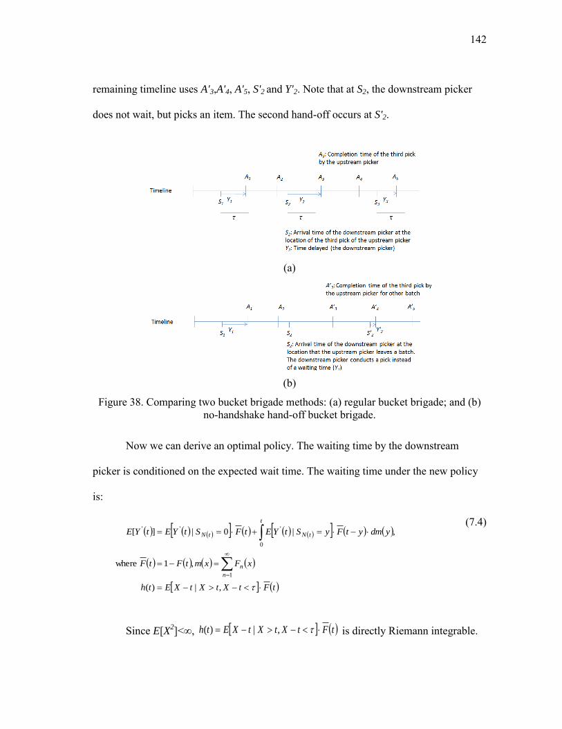
142
remaining timeline uses A'3,A'4, A'5, S'2 and Y'2. Note that at S2, the downstream picker
does not wait, but picks an item. The second hand-off occurs at S'2.
(a)
(b)
Figure 38. Comparing two bucket brigade methods: (a) regular bucket brigade; and (b) no-handshake hand-off bucket brigade.
Now we can derive an optimal policy. The waiting time by the downstream
picker is conditioned on the expected wait time. The waiting time under the new policy
is:
tFtXtXtXEth
xFxmtFtF
ydmytFyStYEtFStYEtYE
n
n
t
tNtN
,|)(
,1 where
,|0|][
1
0
'''
(7.4)
Since E[X2]<∞, tFtXtXtXEth ,|)( is directly Riemann integrable.

143
Thus, we can use the key renewal theorem:
XExdFxdFx
XEdttFtXtXtXEtYE
2/
/,|)]([
2
0
2
0
'
(7.5)
(See Appendix D.4 in detail.)
From Equation (7.5), we derive the following theorem.
Theorem 6. With a no-handshake hand-off policy, the minimum expected hand-
off delay is zero.
Proof.
Equation (7.5) is always greater than and equal to 0 over τ. When τ = 0, this value
is always zero as shown below in Equation (7.6).
02
0
2
xdFxdFx
(7.6)
End of proof.
5. SIMULATION AND EXPERIMENTAL RESULTS
In Sections 3 and 4, analytical and control models were presented to quantify and
reduce picker blocking and hand-off delay. This section will verify the models using
simulations. In addition, the simulations are extended into practical situations since
several assumptions are inevitable in models: no hand-off delay in the picker blocking
model, and a large number of picks and infinite walk speeds in the hand-off models.
More importantly, the performance improvement will be evaluated in practical settings.

144
5.1 Simulation study on picker blocking
Figure 39 illustrates performance loss by picker blocking in 20-pick face bucket
brigade systems and circular picking systems with two pickers whose speed is from 0 to
infinite walk speed. Solid lines are the simulations’ results when pick:walk time = 1:0,
1:0.025, 1:0.05, 1:0.1, 1:0.25, 1:0.5, and 1:1 from top to bottom. The upper dotted line is
an analytical result with pick:walk time = 1: 0. The lower dotted line is a lower bound
with pick:walk time = 1:1. Deterministic pick time and walk speed hold.
When pick:walk time = 1:1, the delay in the bucket brigade picking is almost
identical to the pattern of the circular-aisle picking. When pick:walk time = 1:0, the
bucket brigade order picking faces less blocking than the analytical model and the
circular-aisle model. Our analysis indicates that the 1:0 model can include one hand-off
situation at the first pick face. By chance, as an upstream picker arrives at the first pick
face with a pick, he/she can face a downstream picker. According to the pick-first
priority, the upstream picker picks and the downstream picker waits. Our observation
indicates that when walk speed is not infinite or is unit walk speed, hand-off delay
becomes more of a concern. As hand-off delay arises, the starting time of a new batch is
delayed. Thus, picker blocking decreases.

145
(a) (b)
Figure 39. The percentage of time blocked (two-picker, 20 pick faces) with multiple-picks with infinite backward walk with allowance of intermediate hand-off: (a) bucket brigade system; and (b) circular-aisle system.
5.2 Simulation study on hand-off delay
A simulation study distinguishes when more and less hand-offs occur. The
benefits of the hand-off control strategy are demonstrated.
5.2.1 Impacts on hand-off delay by practical situations
In practice, pickers are neither infinitely fast nor do they process an infinite
number of picks. For a more realistic situation, we analyze the hand-off model using a
discrete-event simulation under the intermediate hand-off rule and pick-first priority.
More specifically, the walk time is classified by forward walk (i.e., loaded walk) and
backward walk (i.e., empty walk) according to the moving direction or the carrying
status of a tote. We consider five situations: 1) 100 pick faces and two pickers with 500
picks and infinite walk speed (notated 2NW-500); 2) 100 pick faces and five pickers
with 50 picks and infinite walk speed (5NW-50); 3) 100 pick faces and five pickers with
20 picks and infinite walk speed (5NW-20); 4) 100 pick faces and five pickers with 20
picks and forward walk time = 0.1 time per pick face (5FW-20); and 5) 100 pick faces
and five pickers with 20 picks, forward walk time = 0.1 time per pick face, and

146
backward walk time = 0.05 time per pick face (5BW-20). Additionally, we consider
three pick time distributions: Uni = uniform [min,max] = [0.5, 1.5], Tri = triangular [min,
mode, max] = [0.5, 1.0, 1.5], and Exp = exponential [mean] = [1.0], where the time unit
represents a time spent to retrieve an item. There are 20 simulation runs with 2000
orders per run; the number of simulation runs is obtained from: 1) the comparison
between our analytical models and simulation results; and 2) the experiment size
proposed by the simulation environments in Ruben and Jacobs (1999).
The comparison results are summarized in Table 12. We are interested in the gap
between analytical results and simulation values over order picking situations. 2NW-500
shows a very small gap compared to the analytical result. As the number of picks
decreases and the number of pickers increases (5NW-50, 5NW-20) the hand-off delay
decreases compared to the analytical value. Forward walk time and backward move also
impact the delay (5FW-20, 5BW-20); less hand-off delay is observed. When walking
takes positive time, pickers can confront each other while walking, not picking
frequently. In this case, a hand-off operation can be conducted without delay. Thus, the
average hand-off delay time is reduced.
Table 12. Average hand-off delay per occurrence over different order picking situations Distribution Uni Tri Exp Time
delayed Gap Time
delayed Gap Time
delayed Gap
Analytical value 0.5466 - 0.5208 - 1.0000 - 2NW-500 0.5419 0.87% 0.5207 0.02% 1.0010 -0.10% 5NW-50 0.5233 4.27% 0.5101 2.06% 0.8663 13.37% 5NW-20 0.4730 13.46% 0.4628 11.14% 0.7046 29.54% 5FW-20 0.3333 39.02% 0.4039 22.46% 0.6253 37.47% 5BW-20 0.3286 39.87% 0.3223 38.13% 0.5225 47.75%
147
5.2.2 No-handshake hand-off policy
A simulation study is conducted to investigate the proposed control methods
including the intermediate hand-off rule. The impact of picker blocking is minimized by
fixing the batch size and only allowing single picks at a given pick face. Several picking
environments are investigated by varying the pick time and the walk time distributions,
the number of pick faces, and workloads.
As depicted in Figure 40, τ = 0 achieves a minimum hand-off delay. While
Figure 40 (a) shows almost zero hand-off delay, Figure 40 (b) shows a relatively
significant hand-off delay in spite of τ = 0. The expected hand-off delay of 5NW-50,
5NW-20, 5FW-20, and 5BW-20 situations in Figure 40 (b) increases as the variance and
range of the pick time distribution increase. In particular, as the number of picks
decreases (5NW-50, 5NW-20 situations in Figure 40 (b)), the values of time delayed
increases when τ = 0. Situations relevant to the pick-first priority for the exponential
pick time cases occur more frequently because the number of picks is too small. When
an upstream picker takes a long time to pick an item, a downstream picker reaches the
hand-off location from the upstream picker before the upstream picker has completed the
first pick. As walking speed impacts the downstream picker’s performance (5FW-20 and
5FW-20 situations in Figure 40 (b)), the time to reach an upstream picker increases; thus
the time delayed decreases when τ = 0. In summary, while a significant portion of the
hand-off delay can be reduced through the no-handshake hand-off rule, the portion of
pick-first priority is exceptional, particularly for the exponential pick time cases in
Figure 40 (b). When the variation of pick time is very high and the number of picks is

148
small, the no-handshake hand-off rule functions poorly. The stable retrieval performance
plays an important role in employing the no-handshake hand-off rule appropriately.
(a) (b)
Figure 40. Impacts on hand-off delay of policy parameter over different picking environments: (a) triangular pick time; and (b) exponential pick time.
5.3 Integrated control of picker blocking and hand-off delay
This section summarizes the computational implementation and discusses
insights from the analysis. IBM and no-handshake hand-off policy are implemented at
different operational levels. IBM is proposed to determine the content of batches and the
sequence of batches, while the no-handshake hand-off policy is an instruction given to
the picker. Instead of integrating the two control strategies, a hierarchical structure is
proposed. The details are as follows:
Use IBM to reduce picker blocking
Teach pickers the no-handshake hand-off policy to reduce hand-off delay
5.3.1 Experimental design
A modified order picking profile based on Koo (2009) is used to evaluate the
proposed procedure. We consider 100 pick faces and five pickers. A picker performs

149
with pick:(forward) walk:backward walk ratio = 1.0:0.1:0.05. We employ a triangular
distribution for pick time. Deterministic forward and backward walk times are assumed.
We compare two control cases: FCFS = sequence orders into batches on a first-come-
first-serve basis and release batches immediately after construction; and Cont = IBM +
no-handshake hand-off operation.
We investigate four different scenarios listed in Table 13. First, a standard
scenario uses the walk speed and picking capability configurations defined above.
Second, a capability scenario differentiates picking capabilities across pickers. The unit
time per pick for the five pickers in the simulation is differentiated into 1.5, 1.25, 1.0,
0.75, 0.5, where an average picker performs one pick per unit time. Third, the fast-walk
scenario looks at the variations in the walk speed of pickers which frequently appear in
the bucket brigade order picking literature (Bartholdi and Eisenstein, 1996b; Koo, 2009),
where the authors assume pickers’ travel with instantaneous walk speed. A fast-walk
situation increases walk speed into pick:walk:back = 1:0.05:0.025; this value is a fast
case in Gue et al. (2006). Fourth, in one small-OPS scenario, the walk speed is fast and
the OPS is small in size. The OPS has 50 pick faces.
We evaluate single order picking and batch order picking. We consider five
scenarios with varying average order sizes of 4, 6, 10, 20, and 50 items for the single
order picking strategy, and two items per order in the batch picking strategy. The order
size of each order is randomly selected based on a uniform distribution [min,max] =
[mean/2, mean*3/2]. Pick time is drawn from a triangular distribution of [min, mode,
max] = [0.5,1.0,1.5]. Note that according to our survey, a practical work load per picker

150
is 2~4 picks per batch (Koo, 2009) and four orders per batch (Bartholdi and Eisenstein,
1996a). Since an order size can vary, but is relatively small in a bucket brigade order
picking, batch picking considers 20 items as a regular batch size (i.e., four picks per
picker or two orders per picker) and 50 items for a heavy demand situation (i.e., 10 picks
per picker or five orders per picker).
As a performance measure, we compare utilization (%), time blocked (%), and
hand-off delay (%). Utilization is the percentage of time spent picking to overall
operations. Time blocked represents a productivity loss. Hand-off delay includes the
ratio of hand-off waiting time to the overall time. In addition, the column labeled Diff in
the result tables (Table 14 and Table 15) shows the comparison between FCFS and Cont.
Run time illustrates the computation time per cycle, where a cycle has k batches for k
pickers.
The simulation is implemented using C language and the IBM formulations using
ILOG CPLEX Callable Library C API 11.0.4. The executable files run on Windows
Server 2008 (Xeon 2.66 Ghz CPU, 12 GB memory, 32 bit implementation). We disable
both the branch-and-cut option and the heuristic search option to evaluate the exact
computational time. One instance includes 2000 orders and 20 runs consistent with
Ruben and Jacobs (1999). The picking environment is summarized in Table 13.
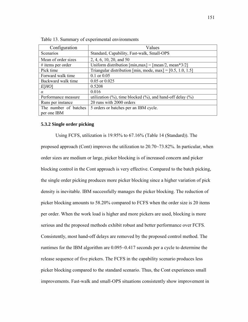
151
Table 13. Summary of experimental environments
Configuration Values Scenarios Standard, Capability, Fast-walk, Small-OPS Mean of order sizes 2, 4, 6, 10, 20, and 50 # items per order Uniform distribution [min,max] = [mean/2, mean*3/2] Pick time Triangular distribution [min, mode, max] = [0.5, 1.0, 1.5] Forward walk time 0.1 or 0.05 Backward walk time 0.05 or 0.025 E[HO] 0.5208 α 0.016 Performance measure utilization (%), time blocked (%), and hand-off delay (%) Runs per instance 20 runs with 2000 orders The number of batches per one IBM
5 orders or batches per an IBM cycle.
5.3.2 Single order picking
Using FCFS, utilization is 19.95% to 67.16% (Table 14 (Standard)). The
proposed approach (Cont) improves the utilization to 20.70~73.82%. In particular, when
order sizes are medium or large, picker blocking is of increased concern and picker
blocking control in the Cont approach is very effective. Compared to the batch picking,
the single order picking produces more picker blocking since a higher variation of pick
density is inevitable. IBM successfully manages the picker blocking. The reduction of
picker blocking amounts to 58.20% compared to FCFS when the order size is 20 items
per order. When the work load is higher and more pickers are used, blocking is more
serious and the proposed methods exhibit robust and better performance over FCFS.
Consistently, most hand-off delays are removed by the proposed control method. The
runtimes for the IBM algorithm are 0.095~0.417 seconds per a cycle to determine the
release sequence of five pickers. The FCFS in the capability scenario produces less
picker blocking compared to the standard scenario. Thus, the Cont experiences small
improvements. Fast-walk and small-OPS situations consistently show improvement in

152
terms of increased utilization.
Table 14. Experimental results on single order picking
5.3.3 Batch order picking
Table 15 summarizes the results of varying the batch size in bucket brigade OPS.
A 4.29~7.04% improvement of utilization in the standard picking situation is observed.
As identified in Section 4, batch picking can reduce the variation of pick density and
lead to less picker blocking. Thus, the results for batch picking are not as dramatic as
observed in the single order picking scenario. Specifically, in the standard situation, the
percentage of time blocked is 1.58~1.68%, whereas the FCFS situation is 2.60~2.89%.
Hand-off control consistently shows improvement; the percentage difference between
FCFS and Cont is 80.70~86.64%. The calculations related to the IBM average 0.387
seconds when the batch size is 20 and 1.254 seconds when the batch size is 50.
Scenarios Order Utilization (%) Time blocked (%) Hand-off delay (%) Run time
Size FCFS Cont Diff (%) FCFS Cont Diff (%) FCFS Cont Diff (%) (seconds)
Standard 4 19.95 20.70 3.75 2.66 1.46 45.09 2.26 0.34 85.15 0.095
6 26.67 28.05 5.17 3.85 1.91 50.41 2.68 0.41 84.67 0.125
10 36.51 38.95 6.67 5.61 2.56 54.38 3.01 0.48 83.92 0.164
20 50.82 55.21 8.64 8.09 3.38 58.20 2.92 0.53 81.97 0.229
50 67.16 73.82 9.92 10.56 3.90 63.05 2.14 0.47 78.09 0.417
Capability 4 19.83 19.97 0.72 1.42 0.82 42.15 2.96 0.23 92.32 0.077
6 26.33 27.06 2.75 1.98 1.03 47.94 3.49 0.26 92.42 0.106
10 36.01 37.67 4.61 2.70 1.38 48.97 3.93 0.34 91.23 0.152
20 50.84 53.90 6.02 3.55 1.74 50.99 3.90 0.46 88.30 0.215
50 69.41 73.29 5.60 4.16 1.84 55.64 2.91 0.49 83.01 0.394
Fast-walk 4 30.58 32.85 7.41 6.81 4.73 30.61 5.13 1.30 74.69 0.148
6 38.42 41.77 8.72 8.27 5.42 34.46 5.35 1.24 76.73 0.187
10 48.49 53.33 9.97 10.01 6.17 38.41 5.12 1.12 78.06 0.230
20 61.32 67.94 10.78 11.48 6.18 46.16 4.18 0.89 78.79 0.277
50 73.92 82.07 11.03 12.44 5.26 57.74 2.55 0.61 76.23 0.463
Small-OPS 4 40.34 44.62 10.62 12.79 11.02 13.81 9.06 3.54 60.97 0.092
6 47.99 53.52 11.51 13.46 11.19 16.85 8.63 2.94 65.90 0.109
10 57.16 64.05 12.06 13.99 10.49 25.01 7.47 2.30 69.17 0.124
20 67.98 76.10 11.94 13.79 8.61 37.54 5.53 1.57 71.64 0.166
50 77.64 86.58 11.51 13.46 6.23 53.68 3.08 0.91 70.36 0.282

153
Interestingly, the proposed approach shows some improvement under capability
instances, where the unit time per pick for the five pickers is not identical and pickers are
optimally sequenced to maximize the picker performance. We note that the capability
instance with batch picking is one of the best-performance order picking situations. Cont
can still give a benefit. Capability instances slightly increase blocking delays, but
achieve large reductions in hand-off delay, and thus lead to overall improvement in
performance.
The fast-walk and small-OPS order picking scenario indicate higher utilization
improvement by the proposed algorithm (3.87~9.45%). Computationally, fast-walk
scenarios experience on average 0.524~1.048 seconds per five batches and small-OPS
scenarios on average 0.338~0.737 seconds.
Table 15. Experimental results varying batch size
5.4 A distance-based heuristic approach for τ
Use of τ as a threshold is not practical in most circumstances since pickers
probably cannot accurately estimate expected hand-off. However, this finding is easily
transferrable to a distance-based heuristic approach. The difficulty of forecasting arises
Scenarios Batch Utilization (%) Time blocked (%) Hand-off delay (%) Run time
Size FCFS Cont Diff (%) FCFS Cont Diff (%) FCFS Cont Diff (%) (seconds)
Standard 20 52.34 56.02 7.04 2.60 1.68 35.34 3.37 0.45 86.64 0.387
50 72.56 75.67 4.29 2.89 1.58 45.28 2.37 0.46 80.70 1.254
Capability 20 51.10 54.29 6.25 1.05 1.06 -1.16 4.10 0.38 90.81 0.236
50 71.66 74.18 3.52 0.78 0.79 -1.68 3.06 0.42 86.37 0.530
Fast-walk 20 64.91 70.39 8.45 4.25 2.81 33.96 5.01 0.71 85.88 0.524
50 81.31 84.64 4.10 3.38 2.29 32.20 2.90 0.64 78.01 1.048
Small-OPS 20 73.03 79.94 9.45 5.94 4.19 29.46 6.51 1.40 78.43 0.338
50 86.34 89.68 3.87 3.81 2.86 24.93 3.25 0.94 70.95 0.737
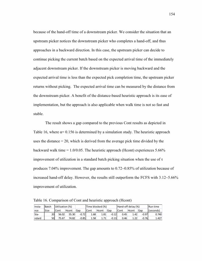
154
because of the hand-off time of a downstream picker. We consider the situation that an
upstream picker notices the downstream picker who completes a hand-off, and thus
approaches in a backward direction. In this case, the upstream picker can decide to
continue picking the current batch based on the expected arrival time of the immediately
adjacent downstream picker. If the downstream picker is moving backward and the
expected arrival time is less than the expected pick completion time, the upstream picker
returns without picking. The expected arrival time can be measured by the distance from
the downstream picker. A benefit of the distance-based heuristic approach is its ease of
implementation, but the approach is also applicable when walk time is not so fast and
stable.
The result shows a gap compared to the previous Cont results as depicted in
Table 16, where α= 0.156 is determined by a simulation study. The heuristic approach
uses the distance = 20, which is derived from the average pick time divided by the
backward walk time = 1.0/0.05. The heuristic approach (Hcont) experiences 5.66%
improvement of utilization in a standard batch picking situation when the use of τ
produces 7.04% improvement. The gap amounts to 0.72~0.85% of utilization because of
increased hand-off delay. However, the results still outperform the FCFS with 3.12~5.66%
improvement of utilization.
Table 16. Comparison of Cont and heuristic approach (Hcont)
Insta- Batch Utilization (%) Time blocked (%) Hand-off delay (%) Run time
nce Size Cont Hcont Gap Cont Hcont Gap Cont Hcont Gap (seconds)
Sta- 20 56.02 55.30 -0.72 1.68 1.81 -0.12 0.45 1.42 -0.97 0.740
ndard 50 75.67 74.82 -0.85 1.58 1.71 -0.13 0.46 1.22 -0.76 1.427
155
6. CONCLUSIONS
This chapter has made three important contributions to the analysis and
understanding of bucket brigade OPS. First, analytical models of picker blocking and
hand-off delay in bucket brigade OPS are developed. Second, based on analytical studies
and additional simulation studies, the conditions are identified under which more
efficient operations can be achieved. Third, control methodologies are developed to
maximize order picking throughput.
Analytical models were developed to quantify the delays related to blocking and
hand-offs by extending the analogy of a circular-aisle OPS to the bucket brigade OPS.
The analytical results found: 1) batch picking can reduce picker blocking because of less
variation of an average work load per batch; and 2) decreased variability in pick time
reduces hand-off delay. Bartholdi and Eisenstein (1996b) emphasized the importance of
a smooth hand-off operation, but did not clearly define the smooth operation and its
rationale. Intermediate hand-off is one method which can reduce delays related to the
hand-off operation. Moreover, the reduction stems from less variance of the expected
pick time of an upstream picker.
Directly controlling picker blocking and hand-off delay also maximizes
throughput. We found that IBM could mitigate picker blocking. Further, the analogy to a
circular-aisle OPS facilitated the development of models to batch orders and assign
batches to pickers to reduce blocking delays in bucket brigade systems. To reduce hand-
off delay, the synchronization requirement in upstream-to-downstream hand-off was
relaxed and strategies to coordinate the physical system were proposed. Both ideal
156
method and practical application were developed.
Based on our findings we suggest that future research should focus upon: 1)
practical application; 2) generalization of the proposed approach for bucket brigades
used in manufacturing operations; and 3) an integrated throughput model. The proposed
methods such as intermedidate hand-off, no-handshake hand-off, and IBM may be
difficult to implement in practice. In the case of the no-handshake hand-off, additional
studies on realistic implementation approaches (e.g., a distance-based heuristic approach)
could be undertaken. Since only order picking systems are considered, the next step is to
identify possible applications in other manufacturing and service areas, for example,
general manufacturing systems such as the assembly line described in Bartholdi and
Eisenstein (2005). A more comprehensive solution that integrates the models could
potentially contribute to a clearer understanding of bucket brigade operation.

157
CHAPTER VIII
CONTRIBUTIONS AND CONCLUSION
Order picking operations play a critical role in the order fulfilment process of
warehouses and DCs. Picking a batch of orders is favored when customers’ demands
create a large number of small orders. Thus, constructing an appropriate order batching
algorithm involves reducing the total retrieval workforce, and differs from a general
batching in that scalability in the number of orders, simplicity in routing, and congestion
must be addressed. This dissertation established four tasks:
First, a large-scale and near-optimal order batching algorithm to minimize the
travel distance is developed. The outcomes of this research highlighted critical
observations of near-optimal, large-scale order batching: less congestion than
expectation, but still significant under some situations.
Second, since the available literature cannot explain the observations, an analysis
and simulation study to identify the complex relationship between sources of
picker blocking and the relevant situations of a real-world firm is undertaken.
Third, a new order batching model and its large-scale solution to manage both
distance and congestion simultaneously is developed.
Fourth, we examined the significance of congestion and hand-off delays in
bucket brigade order picking, followed by providing a structured control
procedure for dynamic order picking which mitigates both picker blocking and
hand-off delay directly.
This dissertation makes three major contributions. First, the proposed analytical
studies give a clear understanding of picker blocking and hand-off delay in batch order
picking. Second, it introduces for the first time in the literature exact batch picking

158
frameworks to handle picker blocking. Third, efficient solution methodologies are
provided for two large-scale, practical order picking situations.
In particular, three new batching models are demonstrated:
1) A near-optimal, large-scale proximity-batching algorithm for traversal routing
methods is developed. We express it as route-selecting batching formulation (RSB). To
obtain an efficient and effective lower bound model for the batching problem, a route-
bin packing problem (RPP) is derived from RSB.
2) A new order batching procedure with picker blocking in a narrow-aisle
picking system is presented (IBM).
3) A new order batching procedure with picker blocking and hand-off delay is
addressed for a bucket-brigade picking system.

159
REFERENCES
Amazon.com (2004) 2003 Amazon.com Annual Report. Amazon.com, Inc., Seattle.
Armbruster, D., Gel, E.S. (2006) Bucket brigades revisted: Are they always effective? European Journal of Operational Research, 172(1), 213-220.
Bartholdi, J.J., Eisenstein, D.D. (1996a) Bucket brigades: a self-organizing order-picking system for a warehouse. Working paper.
Bartholdi, J.J., Eisenstein, D.D. (1996b) A production line that balances itself. Operations Research, 44(1), 21-34.
Bartholdi, J.J., Eisenstein, D.D. (2005) Using bucket brigades to migrate from craft manufacturing to assembly lines. Manufacturing Service Operations
Management, 7(2), 121-129.
Bartholdi, J.J., Eisenstein, D.D., Foley, R.D. (2001) Performance of bucket brigades when work is stochastic. Operations Research, 49(5), 710-719.
Chen, M.-C., Wu, H.-P. (2005) An association-based clustering approach to order batching considering customer demand patterns. Omega, 33(4), 333-343.
Clarke, G., Wright, J.W. (1964) Scheduling of vehicles from a central depot to a number of delivery points. Operations Research, 12, 568-581.
De Koster, R. (2003) Distribution strategies for online retailers. Engineering
Management, IEEE Transactions on, 50(4), 448-457.
De Koster, R. (2004) How To Assess a Warehouse Operation in a Single Tour. RSM Erasmus University, Rotterdam, The Netherlands.
De Koster, R., Balk, B.M. (2008) Benchmarking and monitoring international warehouse operations in Europe. Production and Operations Management, 17(2), 175-183.
De Koster, R., Van der Poort, E.S., Wolters, M. (1999) Efficient orderbatching methods in warehouses. International Journal of Production Research, 37(7), 1479-1504.
De Koster, R., Yu, M. (2008) Minimizing makespan and throughput times at Aalsmeer flower auction. The Journal of the Operational Research Society, 59(9), 9.
Frazelle, E. (2002) World-class Warehousing and Material Handling. McGraw-Hill,

160
New York.
Gademann, N., van de Velde, S. (2005) Order batching to minimize total travel time in a parallel-aisle warehouse. IIE Transactions, 37(1), 63-75.
Gademann, N., Van den Berg, J., Van der Hoff, H. (2001) An order batching algorithm for wave picking in a parallel-aisle warehouse. IIE Transactions, 33(5), 385.
Gong, Y., De Koster, R. (2008) A polling-based dynamic order picking system for online retailers. IIE Transactions, 40, 1070-1082.
Gue, K.R., Meller, R.D., Skufca, J.D. (2006) The effects of pick density on order picking areas with narrow aisles. IIE Transactions, 38(10), 859-868.
Hall, R.W. (1993) Distance approximations for routing manual pickers in a warehouse. IIE Transactions, 25(4), 76.
Ho, Y.C., Tseng, Y.Y. (2006) A study on order-batching methods of order-picking in a distribution centre with two cross-aisles. International Journal of Production
Research, 44(17), 3391-3417.
Hsu, C.M., Chen, K.Y., Chen, M.C. (2005) Batching orders in warehouses by minimizing travel distance with genetic algorithms. Computers in Industry, 56(2), 169-178.
Jane, C.C. (2000) Storage location assignment in a distribution center. International
Journal of Physical Distribution & Logistics Management, 30(1), 55.
Jane, C.C., Laih, Y.W. (2005) A clustering algorithm for item assignment in a synchronized zone order picking system. European Journal of Operational
Research, 166(2), 489-496.
Koo, P.-H. (2009) The use of bucket brigades in zone order picking systems. OR
Spectrum, 31(4).
Law, A.M., Kelton, W.D. (2000) Simulation Modeling and Analysis. McGraw-Hill, Boston.
Le-Duc, T. (2005) Design and control of efficient order picking processes. Ph.D. dissertation, Erasmus University, Rotterdam, The Netherlands.
Le-Duc, T., de Koster, R.M.B.M. (2007) Travel time estimation and order batching in a 2-block warehouse. European Journal of Operational Research, 176(1), 374-388.
Lewis, R.T., Parker, R.G. (1982) On a generalized bin-packing problem. Naval Research
Logistics Quarterly, 29(1), 119-145.
161
Lieu, C.C.A. (2005) Impact of inventory storage and retrieval schemes on productivity. MBA. and MS. thesis, Massachusetts Institute of Technology, Cambridge, MA.
Lim, Y.F., Yang, K.K. (2009) Maximizing throughput of bucket brigades on discrete work stations. Production and Operations Management, 18(1), 48-59.
Napolitano, M. (2008) Sitting tight - 2008 warehouse/DC operations survey results. Logistics Management, 47(11), 47-50.
Napolitano, M. (2009) Real DC stories: low cost deep impact. Logistics Management, 48(1), 46-49.
Napolitano, M., Gross&Associates (2003) The Time, Space and Cost Guide to Better
Warehouse Design. The Distribution Group, Ogden, UT.
Pan, C.H., Liu, S.Y. (1995) A comparative study of order batching algorithms. Omega, 23(6), 691-700.
Parikh, P.J., Meller, R.D. (2009) Estimating picker blocking in wide-aisle order picking systems. IIE Transactions, 41, 232-246.
Parikh, P.J., Meller, R.D. (2010) A note on worker blocking in narrow-aisle order picking systems when pick time is non-deterministic. IIE Transactions, 42(6), 392 - 404.
Petersen, C.G. (1997) An evaluation of order picking routeing policies. International
Journal of Operations & Production Management, 17(11), 1098-1111.
Petersen, C.G. (2000) An evaluation of order picking policies for mail order companies. Production and Operations Management, 9(4), 319-335.
Petersen, C.G., Schmenner, R.W. (1999) An evaluation of routing and volume-based storage policies in an order picking operation. Decision Sciences, 30(2), 481-501.
Pinedo, M. (1995) Scheduling: Theory, Algorithms, and Systems. Prentice Hall, Englewood Cliffs, NJ.
Ratliff, H.D., Rosenthal, A.S. (1983) Order-picking in a rectangular warehouse: a solvable case of the traveling salesman problem. Operations Research, 31(3), 507-521.
Roodbergen, K.J., de Koster, R. (2001) Routing methods for warehouses with multiple cross aisles. International Journal of Production Research, 39(9), 1865-1883.
Ross, S.M. (1996) Stochastic Processes. John Wiley & Sons, Inc., New York.

162
Ruben, R.A., Jacobs, F.R. (1999) Batch construction heuristics and storage assignment strategies for walk/ride and pick systems. Management Science, 45(4), 575-596.
Skufca, J.D. (2005) k Workers in a circular warehouse: a random walk on a circle, without passing. SIAM Review, 47(2), 301-314.
Tompkins, J.A., Bozer, Y.A., Tanchoco, J.M.A. (2003) Facilities Planning. J. Wiley, Hoboken, NJ.
Wilson, R. (2008) 19th Annual State of Logistics Report. Council of Supply Chain Management Professionals, Washington DC.
Won, J., Olafsson, S. (2005) Joint order batching and order picking in warehouse operations. International Journal of Production Research, 43(7), 1427-1442.
Yu, M., De Koster, R.B.M. (2009) The impact of order batching and picking area zoning on order picking system performance. European Journal of Operational
Research, 198(2), 480-490.
Zhang, M., Batta, R., Nagi, R. (2009) Modeling of workflow congestion and optimization of flow routing in a manufacturing/warehouse facility. Management
Science, 55(2), 267-280.

163
APPENDIX A
SUPPLEMENTARY FORMULATION, PROOF, ALGORITHM,
AND RESULTS DISCUSSED IN CHAPTER IV
A.1 FORMULATION OF BASIC RPP FROM RSB
The basic RPP can be derived from RSB. In particular, each constraint in the
basic RPP is derived from a constraint of RSB, or becomes a constraint aggregating
relevant constraints in RSB.
1) Objective function
Rr
rr
Rr Bb
brr
Bb Rr
brr
yLT
YLTYLT
By definition, r
Bb
br yY
2) Constraints (4.8)
From (4.2),
1Bb
ob X Oo
1. . .||21
Bobobob XXX Oo
1...||||2211
Rr
rbob
Rr
rbob
Rr
rbob BBYXYXYX Oo Since 1
Rr
brY
1...||||2211
Rr
rbob
Rr
rbob
Rr
rbob BBYXYXYX Oo
1)...(||||2211
YXYXYX
Rr
rbobrbobrbob BB Oo
1)(
YX
Rr Bb
brob Oo By definition,
o r
Bb
b ro b xYX
1Rr
or x Oo

164
3) Constraints (4.9)
From (4.3),
,
,
,
CAPA XQ
CAPA XQ
CAPA XQ
Oo
obo
Oo
obo
Oo
obo
BbYbBb
BbYbBb
BbYbBb
RbrR
br
br
,1|
,1|
,1|
||
2
1
||
2
1
Assume that all b’s have at least one order
,
,
,
||||
22
11
RR br
Oo
brobo
br
Oo
brobo
br
Oo
brobo
YCAPA YXQ
YCAPA YXQ
YCAPA YXQ
||
2
1
RBb
Bb
Bb
By definition,
1rbrY
,
,
,
||
||
||
||
2
2
2
2
1
1
1
1
R
R
R
R
Bb
br
Bb Oo
brobo
Bb
br
Bb Oo
brobo
Bb
br
Bb Oo
brobo
YCAPA YXQ
YCAPA YXQ
YCAPA YXQ
Aggregate constraints indexed by r. The new constraints become weaker, thus the new model becomes a relaxation of the original constraints
rr Bb
br
Oo Bb
brobo YCAPA YXQ Rr
,r
Oo
oro yCAPA xQ
Rr
By definition, o r
Bb
b ro b xYX
and
r
Bb
br yY
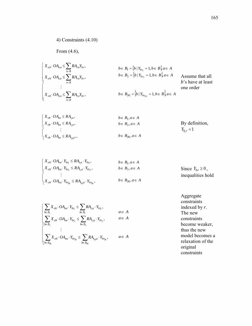
165
4) Constraints (4.10)
From (4.6),
,
,
,
Rr
brraoaob
Rr
brraoaob
Rr
brraoaob
YRAOAX
YRAOAX
YRAOAX
AaBbYbBb
AaBbYbBb
AaBbYbBb
RbrR
br
br
, ,1|
, ,1|
, ,1|
||
2
1
||
2
1
Assume that all b’s have at least one order
,,
,
,
||
2
1
aroaob
aroaob
aroaob
RRAOAX
RAOAX
RAOAX
AaBb
AaBb
AaBb
R
,
,
,
||
2
1
By definition, 1rbr
Y
,
,
,
||||||
222
111
RRR brarbroaob
brarbroaob
brarbroaob
YRAYOAX
YRAYOAX
YRAYOAX
AaBb
AaBb
AaBb
R
,
,
,
||
2
1
Since 0brY , inequalities hold
,
,
,
||
||||
||
||
2
22
2
2
1
11
1
1
R
RR
R
R
Bb
brar
Bb
broaob
Bb
brar
Bb
broaob
Bb
brar
Bb
broaob
YRAYOAX
YRAYOAX
YRAYOAX
Aa
Aa
Aa
Aggregate constraints indexed by r. The new constraints become weaker, thus the new model becomes a relaxation of the original constraints

166
,
,
,
||
||||
||
||
2
22
2
2
1
11
1
1
R
RR
R
R
Bb
brar
Bb
broboa
Bb
brar
Bb
broboa
Bb
brar
Bb
broboa
YRAYXOA
YRAYXOA
YRAYXOA
Aa
Aa
Aa
,
rr Bb
brra
Bb
broboa YRAYXOA AaRr ,
,rraoroa yRAyOA AaRr ,
By definition, o r
Bb
b ro b xYX
and r
Bb
br yY
A.2 CLARKE AND WRIGHT II ALGORITHM (CLARKE AND WRIGHT, 1964;
DE KOSTER ET AL., 1999)
Step 1. Obtain the distance savings sij for all possible order pairs i,j when two
orders are grouped, given the capacity of the pick device.
Step 2. Sort the savings in decreasing order.
Step 3. Select the pair with the highest savings. In the case of a tie, select a
random pair.
Step 4. Combine both ―orders‖ to form a new cluster, if allowed by the pickers’
capacity. If not, choose the next combination on the list and repeat step 4.
Step 5. If not all order combinations have been included in a route, proceed with
Step 1. In the calculation, all clusters are considered as orders. Otherwise,
finish.

167
A.3 SIMULATED ANNEALING PROCEDURE FOR RBP
This section presents a simulated annealing algorithm for order batching to
obtain an improved solution from RBP and summarizes the experimental results.
Simulated annealing procedure
Simulated annealing is widely used in sequencing problems and order batching
problems. We employ an algorithm described in Pinedo (1995). For a batching situation,
a batching solution is given as BS1 and its total retrieval time as Obj(BS1). The major
characteristic is to accept a worse solution (BS) while progressively searching for a
better candidate solution of solution BSi with probability P(BSi,BS) = e^( (Obj(BSi)-
Obj(BS)/ βi ), where βi is referred to as the cooling parameter or temperature. To update
the cooling parameter (βi), we use a simple function ai where 0<a<1, a ∈ R (see Pinedo
(1995) in detail). Thus, the probability to admit an solution with a worse objective value
is gradually decreases as iteration i cumulatively updates the cooling parameter (βi)
using a, i.e., βi= a*βi-1 where i>1 and 0<a<1. To generate an initial solution (BS1), RBP
is used, which produces a solution that nearly minimizes the total retrieval distance. Imax
is the maximum number of iterations. T is the updated temperature.
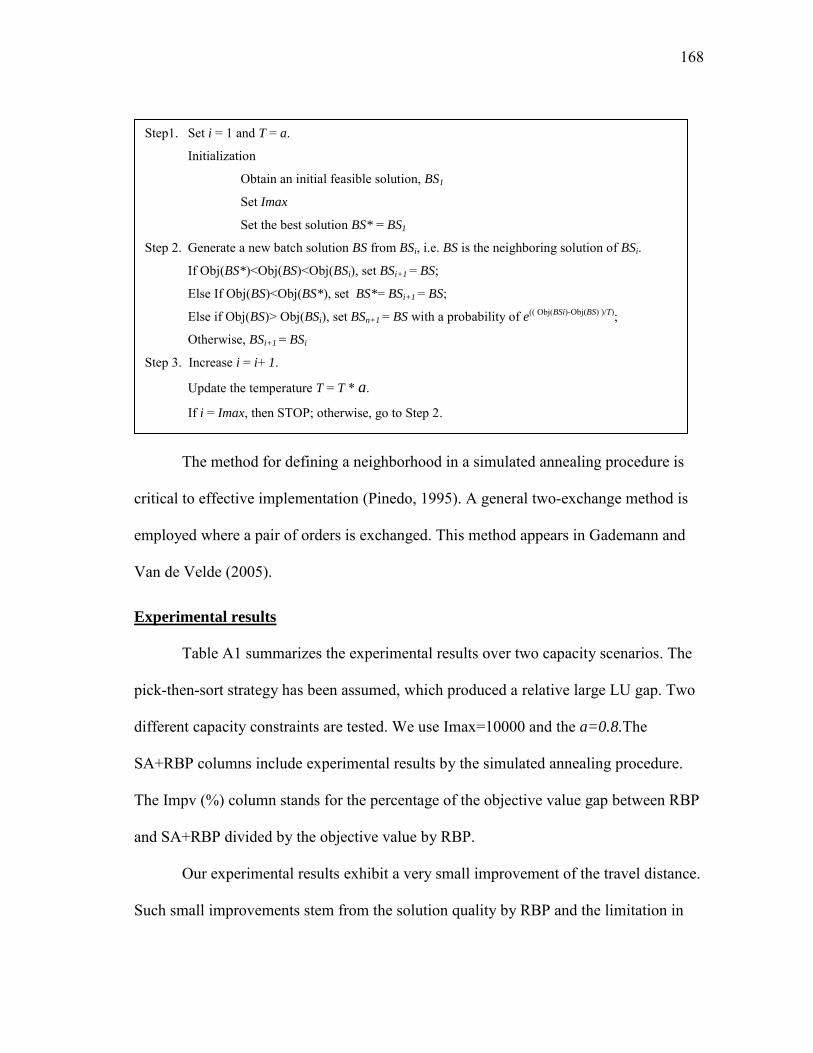
168
The method for defining a neighborhood in a simulated annealing procedure is
critical to effective implementation (Pinedo, 1995). A general two-exchange method is
employed where a pair of orders is exchanged. This method appears in Gademann and
Van de Velde (2005).
Experimental results
Table A1 summarizes the experimental results over two capacity scenarios. The
pick-then-sort strategy has been assumed, which produced a relative large LU gap. Two
different capacity constraints are tested. We use Imax=10000 and the a=0.8.The
SA+RBP columns include experimental results by the simulated annealing procedure.
The Impv (%) column stands for the percentage of the objective value gap between RBP
and SA+RBP divided by the objective value by RBP.
Our experimental results exhibit a very small improvement of the travel distance.
Such small improvements stem from the solution quality by RBP and the limitation in
Step1. Set i = 1 and T = a.
Initialization
Obtain an initial feasible solution, BS1
Set Imax
Set the best solution BS* = BS1
Step 2. Generate a new batch solution BS from BSi, i.e. BS is the neighboring solution of BSi.
If Obj(BS*)<Obj(BS)<Obj(BSi), set BSi+1 = BS;
Else If Obj(BS)<Obj(BS*), set BS*= BSi+1 = BS;
Else if Obj(BS)> Obj(BSi), set BSn+1 = BS with a probability of e(( Obj(BSi)-Obj(BS) )/T);
Otherwise, BSi+1 = BSi
Step 3. Increase i = i+ 1.
Update the temperature T = T * a.
If i = Imax, then STOP; otherwise, go to Step 2.
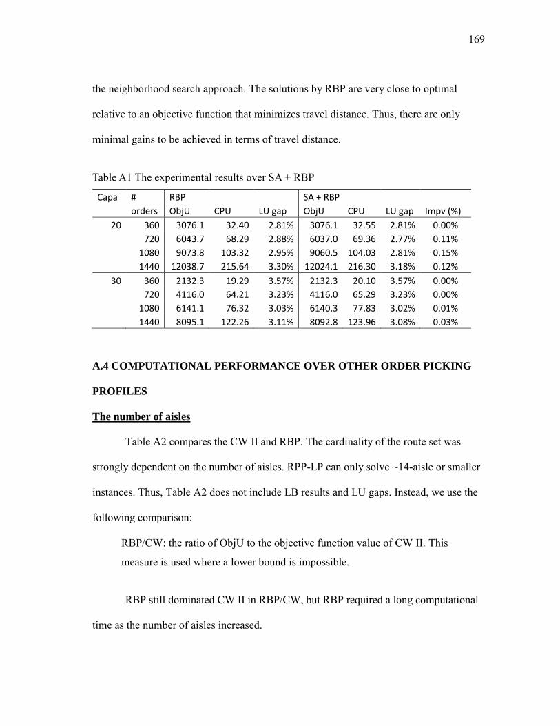
169
the neighborhood search approach. The solutions by RBP are very close to optimal
relative to an objective function that minimizes travel distance. Thus, there are only
minimal gains to be achieved in terms of travel distance.
Table A1 The experimental results over SA + RBP
Capa # RBP SA + RBP orders ObjU CPU LU gap ObjU CPU LU gap Impv (%)
20 360 3076.1 32.40 2.81% 3076.1 32.55 2.81% 0.00% 720 6043.7 68.29 2.88% 6037.0 69.36 2.77% 0.11% 1080 9073.8 103.32 2.95% 9060.5 104.03 2.81% 0.15%
1440 12038.7 215.64 3.30% 12024.1 216.30 3.18% 0.12%
30 360 2132.3 19.29 3.57% 2132.3 20.10 3.57% 0.00% 720 4116.0 64.21 3.23% 4116.0 65.29 3.23% 0.00% 1080 6141.1 76.32 3.03% 6140.3 77.83 3.02% 0.01% 1440 8095.1 122.26 3.11% 8092.8 123.96 3.08% 0.03%
A.4 COMPUTATIONAL PERFORMANCE OVER OTHER ORDER PICKING
PROFILES
The number of aisles
Table A2 compares the CW II and RBP. The cardinality of the route set was
strongly dependent on the number of aisles. RPP-LP can only solve ~14-aisle or smaller
instances. Thus, Table A2 does not include LB results and LU gaps. Instead, we use the
following comparison:
RBP/CW: the ratio of ObjU to the objective function value of CW II. This
measure is used where a lower bound is impossible.
RBP still dominated CW II in RBP/CW, but RBP required a long computational
time as the number of aisles increased.

170
Table A2 The experimental results with the variation of the number of aisles
# # CW II RBP
orders aisles Obj CPU ObjL ObjU CPU # routes RBP/CW
1080 10 8033.3 15.6 7175.0 7175.0 56.7 40.4 0.89
20 12492.8 17.0 10647.5 10647.5 121.0 147.2 0.85
30 16614.3 17.2 14379.6 14379.6 242.9 254.4 0.87
40 20517.8 18.7 18418.0 18418.0 366.8 342.4 0.90
2160 10 15412.0 141.5 14186.6 14186.6 60.5 47.8 0.92
20 23365.4 129.5 20287.7 20287.7 123.1 214.1 0.87
30 31102.9 147.8 26587.4 26587.4 253.5 393.4 0.85
40 37971.8 142.0 33637.3 33637.3 394.3 552.9 0.89
The route reduction step is not effective in the 40-aisle instance. As the number
of routes increased, we modulated the truncation time limit to produce good solutions;
specifically, 120 seconds, 180 seconds, and 240 seconds were allowed for 20-aisle, 30-
aisle, 40-aisle instances. However, despite this increase in the truncation time limit,
RBP’s performance suffered loss in the objective values. Figure A1 illustrates the
variations of the average travel length over different algorithms with respect to the
number of aisles. The performance gap between CW II and RBP did not widen as shown
in Figure A1 when the number of aisles was 40.
(a) (b)
Figure A1 The average travel length per order over the variation of the number of aisles: (a) the number of orders = 1080, and (b) the number of orders = 2160.

171
Storage policy
Table A3 and Figure A2 include the test results with different storage policies.
Picking systems can operate under different storage pattern or storage policies As orders
were scattered more evenly, all algorithms had longer travel distance. In particular, the
computational time of RBP lengthened. The storage policy has an impact on the route set
of RBP. More uniformly-stored items produce more elementary routes. Thus, the
elementary route set becomes larger, and the number of combined routes also increases.
A larger route set results in longer computational time.
Table A3 The experimental results with the variation of storage policies
# # CW II RBP Orders aisles Obj CPU ObjL ObjU CPU # routes RBP/CW
ABC 10 18000.4 140.8 16181.4 16181.4 60.7 63.7 0.90 =0.5:0.3:0.2 20 28926.6 130.9 24043.8 24043.8 128.4 340.5 0.83 30 38950.5 134.7 33104.8 33104.8 278.7 581.6 0.85 40 47811.1 151.0 42441.0 42441.0 568.7 747.8 0.89
Random 10 22125.6 121.3 19310.4 19310.4 60.9 83.0 0.87 Storage 20 37872.4 126.9 34535.9 34535.9 150.0 554.5 0.91 30 51343.2 138.2 46266.7 46266.7 347.9 796.4 0.90 40 63794.8 155.1 57098.8 57098.8 699.6 901.9 0.90
(a) (b)
Figure A2 The average travel length per order over the variation of the storage policy (# orders = 1080): (a) ABC ratio = 0.5:0.3:0.2; and (b) random storage policy.

172
APPENDIX B
SUPPLEMENTARY EXAMPLES, PROOF, VALIDATION, ALGORITHM, AND
RESULTS DISCUSSED IN CHAPTER V
B.1 PICKER BLOCKING MODEL OF PICK:WALK TIME = 1:1 IN A
NARROW-AISLE USING PICK AND WALK TASKS
Let Dt denote the distance between picker 1 and picker 2 at time t. Given the
pick:walk time ratio as 1:1, the distance d can be expressed as
(n+(picker 1 position)−(picker 2 position)) mod n
and ranges from 1 to n-1. To establish a Markov property, we can condition on the either
pick or walk state of a previous distance and connect to the either pick or walk state of a
posterior distance. Since there are two pickers and they can conduct either pick or walk,
four sub states are available: dpp, dwp, dpw, dww depending on the actions of pickers 1 and
2 and distance d, where p stands for a picking, w for a walking. In particular, two states,
1wp and n-1pw are augmented into ―blocked‖ because one picker attempts to walk toward
one occupied pick face. Then all states can be described as the states [1pp, 1pw, blocked,
1ww, 2pp, 2pw, 2wp, 2ww, . . . , (n − 1)pp, blocked, (n − 1)wp, (n − 1)ww]. When multiple-picks
are allowed, their transition probability forms a new relationship. Figure A3 illustrates
the transitions.
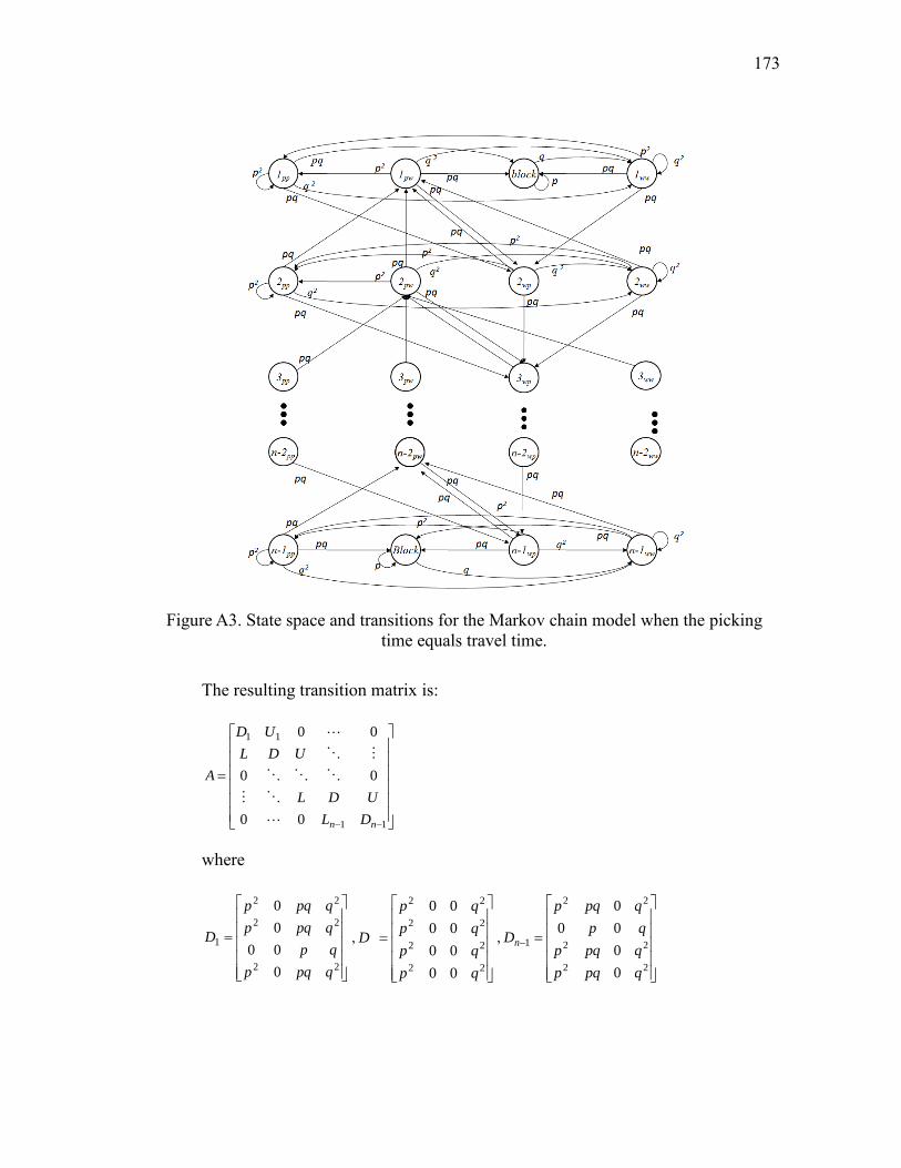
173
Figure A3. State space and transitions for the Markov chain model when the picking time equals travel time.
The resulting transition matrix is:
11
11
00
00
00
nn DL
UDL
UDL
UD
A
where
22
22
22
1
0
00
0
0
qpqp
qp
qpqp
qpqp
D ,
22
22
22
22
00
00
00
00
qp
qp
qp
qp
D ,
22
22
22
1
0
0
00
0
qpqp
qpqp
qp
qpqp
Dn

174
000
0000
000
000
1
pq
pq
pq
U ,
000
000
000
000
pq
pq
pq
pq
U ,
000
000
000
000
pq
pq
pq
pq
L ,
000
000
0000
000
1
pq
pq
pq
Ln
Similar to Gue et al. (2006), we obtain the following v which satisfies vA=v.
1
2
2
22
2
22
1
2 ,,,,21,,,,,21,,,,,,
ndnddd
qpqpppppppppp,ppqppqpv
We can scale the stationary density using ||v||.
12
123
2213 222
pn
pn
qppqppppppnv
The blocking probability of picker 2 is
122 3
1:1
pn
p
v
vbm
B.2 PICKER BLOCKING WHEN PICK:WALK TIME = 1:1 IN A WIDE-AISLE
A Markov property is applied in pick:walk time = 1:1 for a wide-aisle situation.
When multiple picks are allowed, their transition probability forms a transition diagram
as illustrated in Figure A4.
Figure A4. State space and transitions for the Markov chain model when picking time
equals travel time in a wide-aisle situation with multiple-pick allowance.

175
The resulting transition matrix which has (n+1) x (n+1) is:
22
22
22
22
22
000
000
000
000
002
0002
qpqqpq
pqqppq
pqqp
qppq
pqpqqp
qqp
A
Stationary distribution
We obtain the following v which satisfies vA = v:
222 2
1,,
2
1,,1
p
q
p
q
p
qv
We can scale the stationary density using ||v|| to obtain a stationary probability.
From v above, we have:
2
2
2
2
2
2
2
2
22
2
22
2
22)1(22
2
2122
2
1122
2
111
p
pnpp
p
ppnnpp
p
pnqp
p
qnqp
p
qn
p
qv
The blocking probability of blocking state of a picker is
pnpp
p
p
pnppv
vb
22
2
22
2
1
22
2
2
2
*1 (A1)

176
B.3 PROOF OF PROBABILITY WITHOUT PASSING
q
pq
pq
qpqqpq
pqpqpq
xfyxfxYPyxYP
yYPyg
y
yy
x
xy
x
yx
x
xyx
xx
tt
t
1
111
1
2
2
2
0
22
0
22
0
00
B.4 COMPARISON OF ANALYTICAL AND SIMULATION MODELS
Table A4 summarizes the results to validate the new analytical models and our
simulation models. The 1:1 analytical model is already identical to the model by Parikh
and Meller (2010). The results by the 1:0 analytical models also experienced
0.032~0.170% error gap compared to the results of Parikh and Meller (2010). The gap
between the performances of the simulation model and the analytical model is 0.01~0.33%
in terms of the percentage of the difference of the percentage of time blocked (i.e., Diff %
= (the percentage of time blocked by the analytical model – the percentage of time
blocked by the simulation model)/(the percentage of the time blocked by the analytical
model) * 100) except one instance. When picker blocking occurs rarely, for example
when p = 0.05 in pick:walk time = 1:1, the simulation model gives a relatively higher
difference. For other cases, the difference percentage is smaller than 0.33%. These
results show that the analytical model can well estimate a multiple-pick blocking
situation.

177
Table A4. Comparison of analytical and simulation results of the percentage of time blocked in a circular aisle (20 pick faces)
B.5 CLARKE AND WRIGHT II ALGORITHM (CLARKE AND WRIGHT, 1964;
DE KOSTER ET AL., 1999)
Step 1. Obtain the distance savings sij for all possible order pairs i,j when two orders
are grouped, given the capacity of the pick device.
Step 2. Sort the savings in decreasing order.
Step 3. Select the pair with the highest savings. In the case of a tie, select a random
pair.
Step 4. Combine both orders to form a new cluster, if allowed by the pickers’
capacity. If not, choose the next combination on the list and repeat Step 4.
Step 5. If all order combinations have not been included in a route, proceed with Step
1. In the calculation, all clusters are considered as orders. Otherwise, finish.
B.6 A HEURISTIC ROUTE-PACKING BASED ORDER BATCHING
PROCEDURE (RBP)
RBP takes advantage of the traversal routing method. When traversal routing
Probability Pick:walk time =1:1 Pick:walk time =1:0
p Analytical Simulation Diff % Analytical Simulation Diff %
0.05 0.2618 0.2580 1.43 33.8983 33.8823 0.05
0.1 0.5208 0.5225 -0.33 25.6410 25.6283 0.05
0.2 1.0309 1.0313 -0.03 17.2414 17.2454 -0.02
0.3 1.5306 1.5256 0.33 12.9870 12.9916 -0.04
0.4 2.0202 2.0186 0.08 10.4167 10.4181 -0.01
0.5 2.5000 2.5005 -0.02 8.6957 8.6871 0.10
0.6 2.9703 2.9655 0.16 7.4627 7.4567 0.08
0.7 3.4314 3.4243 0.21 6.5359 6.5327 0.05
0.8 3.8835 3.8749 0.22 5.8140 5.8007 0.23
0.9 4.3269 4.3154 0.27 5.2356 5.2224 0.25
0.95 4.5455 4.5491 -0.08 4.9875 4.9917 -0.08

178
methods are used, all possible routes can be constructed from the warehouse layout.
Thus, given a batch, a best fit route can be selected as a bin-packing problem (called the
route-selecting order batching model (RSB)).
RBP is composed of three steps:
Step 1. Identifies potential route sets.
Step 2. Solves the RPP model heuristically. The RSB model stated above simplifies
the batching problem, but still contains partitioning constraints. A route-bin
packing problem (RPP) is developed by assigning orders to routes directly,
which can skip the partitioning stage. However, RPP is still computationally
difficult, and thus we consider two further computational improvements: a
partial route set and a truncated branch-and-bound approach.
Step 3. Restores a feasible solution from the infeasible solution by the relaxed model.

179
APPENDIX C
EXECUTABLE MIP FORMULATION FOR INDEXED BATCH
MODEL
Decision variables
,,, aif
aif
aif DICDD
= the time delay of the ith batch at pick face f in aisle a, its cumulative
time delay, and its intermediate variable
,,, ai
aif
aif LFLIL
= the leaving time of the ith batch at pick face f in aisle a
Formulation
Min
Aa Bb
a
FiBb
bb CDAWRBAWTAHNBANBVUTLT a22
s.t
,1Bb
ob X O, o
,CAPA X
Oo
o b
B, b
obb XBV
B, bO, o
Oo
obb XBV
B, b
1 bb BVBV
,BB b \
Bb
bBVNBV
, Oo
bfobbf OPXPTBP
F, fB, b
oboaba XOAVBA
A, aB, bO, o
ba
ak
bkbaba
ba
ak
bkbaba
BAaBABAMINT
BAaBABAMINT
,..,0
,..,0
112
112
B bA a ,

180
,2
Aa
bab BANBA B, b
,bab BAaRBA B, b
,1
,...,
Aak
bkbkb BAMBAkRBA B, b
NPik
k ii APMSTLTCW,...,1
00 1
00, ,a fB, bNPi
NPik
k ii APMSTLTCW,...,1
00 1
00, ,a fB, bNPi
kkii APMCTLTCW 100
00 , ,a fB,iNPk
kkii APMCTLTCW 100
00 , ,a fB,iNPk
aijj,a
aif YMAWBACCW 11
,Aa fB,j i 0\,0,
aijj,a
aif YMAWBACCW 11
,Aa fB,j i 0\,0,
afi
ai
aif CWAVWTCW 1,
,Aa
F fB,j i a
0\
,,
,1,a
fba
ifa
if CPPCP
A,aF fB, i a ,
, 001,ai
ai
afi
aif
aif DCDCDDCD
A,a
F fM i a
,0 ,
aif
aif
aif
aif
aif
aif
aif
aif
aif
aif
aif
aif
aif
aif
a
afi
aif
aif
afi
aif
afi
aif
DFMDI
DFMDI
DFMDXDI
DFMDXDI
DFMDX
DFMDX
FffWTCDCW
CPL
fAECWL
DX
1
1
1
0
and 0 if
0 if
otherwise1,
1,1
1,1
A,a
F fB, i a
,0
ai
aif AVMD
A,a
F fB, i a
,0
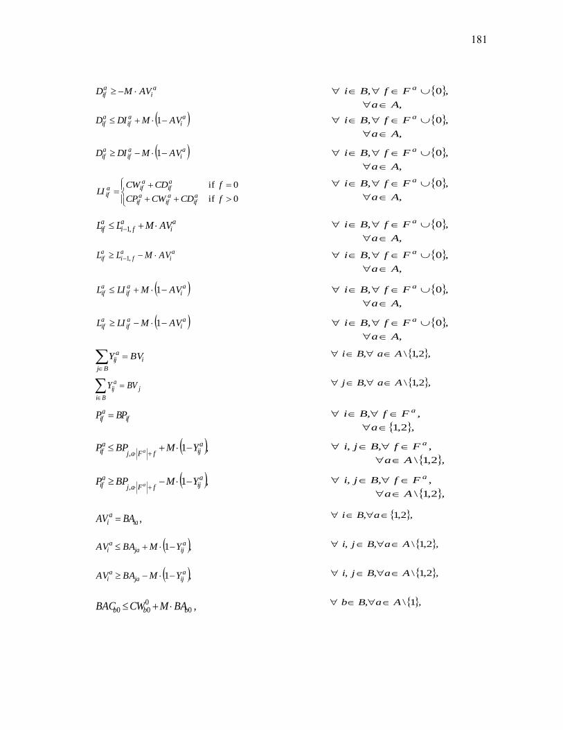
181
ai
aif AVMD
A,a
F fB, i a
,0
ai
aif
aif AVMDID 1
A,a
F fB, i a
,0
ai
aif
aif AVMDID 1
A,a
F fB, i a
,0
0 if
0 if
fCDCWCP
fCDCWLI
aif
aif
aif
aif
aifa
if
A,a
F fB, i a
,0
ai
afi
aif AVMLL ,1
A,a
F fB, i a
,0
ai
afi
aif AVMLL ,1
A,a
F fB, i a
,0
ai
aif
aif AVMLIL 1
A,a
F fB, i a
,0
ai
aif
aif AVMLIL 1
A,a
F fB, i a
,0
iBj
aij BVY
,A aB, i 2,1\
j
Bi
aij BVY
,A aB, j 2,1\
if
aif BPP
,a
F fB, i a
2,1
,
,1,
aijfFaj
aif YMBPP a
,Aa
F fB,j i a
2,1\
,,
,1,
aijfFaj
aif YMBPP a
,Aa
F fB,j i a
2,1\
,,
,iaa
i BAAV
,aB, i 2,1
,1 aijja
ai YMBAAV
,AaB,j i 2,1\,
,1 aijja
ai YMBAAV
,AaB,j i 2,1\,
, 0000 bbb BAMCWBAC ,AaB, b 1\

182
, 0000 bbb BAMCWBAC ,AaB, b 1\
, 1 00
0 0 bFbb BAMAE LBAC ,AaB, b 1\
,BAMAE LBAC bFbb 00
0 10 ,AaB, b 1\
,1 bab,a-ba BAMAWBACBAC
,AaB, b 1\
,1 bab,a-ba BAMAWBACBAC
,AaB, b 1\
,1 baa
bba BAMWTLFBAC
,AaB, b 1\
,1 baa
bba BAMWTLFBAC
,AaB, b 1\
,1,
aib
a
Fi
ab YMLLF a
,AaB,b i 1\,
,1,
aib
a
Fi
ab YMLLF a
,AaB,b i 1\,
1,11,
1,
11
1
ia
jiaj
aijaj
BVMYMBAC
YMBAC
,AaB,j i 2,1\, i
Bj
ij BVZ
B, i
jBi
ij BVZ
B, i
ij
jiAji
ZMUT
AWRBAAWRBAABACCT
1
11,
B,j i ,
ij
jiAji
ZMUT
AWRBAAWRBAABACCT
1
11,
B,j i ,
11 1 iii BVM CTCT
,BB i \

183
APPENDIX D
SUPPLEMENTARY FORMULATIONS AND PROOFS DISCUSSED IN
CHAPTER VII
D.1 PACKING PROBLEM
The goal is to minimize the number of batches (A2). Yb is 0 if batch b is selected
and 0 otherwise. (A3) forces one order to be assigned once. (A4) is used to meet a
capacity constraint if necessary.
Min Bb
bY (A2)
s.t.
1Bb
obX
O, o (A3)
bOo
obo YCAPAXOS
B, b (A4)
D.2 INDEXED BATCHING MODEL (IBM) FOR BUCKET BRIGADE ORDER
PICKING
Parameters and decision variables
An OPS has a linear aisle with |F| pick faces. The pick faces are numbered 1 to F.
L/U stations are numbered 0 and F+1, respectively. The forward travel time between
neighboring pick faces is WT. The backward travel time between neighboring pick faces
is BW. The walk time from 0 to F+1 is equal to WT*(|F|+1) = AH. The L/U stations are

184
located in the front and rear of the aisle.
NP pickers work in the OPS, and the OPS is forced to assign all pickers. The
number of batches is not given, although the number of batches must be smaller than the
number of orders. Generally, the number of batches is greater than the number of pickers.
Two batching picking policies — pick-then-sort policy and sort-while-pick policy — are
considered; the policy impacts cart capacity. When a batch is completed, a new batch
enters the system. Its entrance time is updated based on the backward walk time and the
expected hand-off delay. All pickers are available initially.
Diverse decision variables are associated with the indexed order batching
problem. Fundamentally, orders are assigned to batches and their release orders through
index variables (Xoi). The starting time of batches in a picker’s second or more trips (CWi)
is updated. The overall procedure includes more variables.
Indices and parameters
fF , = the set of pick faces, its index f ∈ F oO, = the set of orders, and its index o∈O iB, = the set of batches, and its index i∈ B
ofOP = the number of picks of order o at pick face f
oOS = the number of picks in order o
iST = the starting time of ith batch
CAPA = the capacity of a cart (batch size)
PT = the pick time to pick an item
WT = the forward walk time between two pick faces
BW = the backward walk time between two pick faces

185
HOE = the expected hand-off delay per occurrence
NP = the number of pickers
= the weight on hand-off delay = the time required for the transition between two batches in a pick face
Decision variables
oiX = 1 if order o enters the ith order; 0 otherwise
ifif CPP ,
= the pick time of the ith batch at pick face f, and its cumulative pick time
ifif CDD ,
= the time delayed of the ith batch at pick face f, and its cumulative time delayed
ifCW
= the cumulative walk time of the ith batch to pick face f
iCT = the completion time of the order which has finished at the ith batch
The goal is to minimize total walk time + total time delayed (A5). Walk time is
the sums of the travel times of all batches. The travel time of the ith batch is the sum of
the forward travel times (= AH*WT), the backward travel times (= AH*BW) if i >PK,
and the hand-off time if i >PK. DT is obtained by summing the cumulative delay at the
last pick face of all batches.
Min
NBVbFi
CDPKBHOENPBWAHBWTAH
,,1
][1
(A5)
s.t.
1Bi
oiX
O, o (A6)
CAPAXOSOo
oio
B, i (A7)

186
, Oo
ofoiif OPXPTP
F, fB, i (A8)
0
0 , if][1
0 , if
1,
,,,
fWTCW
fNPiHOENPFBW
CDCWCP
fNPiST
CW
fi
FNPiFNPiFNPi
i
if
,F fB, i 0 (A9)
,1, fiifif CPPCP
, F fB, i (A10)
, 001, iifiifif DCDCDDCD
0 F fB, i (A11)
otherwise0
},0{\ 0,
0 if0,
1,11,11,1
1,11,1
FFfWTCDCWCP
CDCWCPMax
fCWCDCWMax
D a
ififif
fififi
ififi
if
0 , F fB i (A12)
An order cannot be separated (A6) and a batch should keep the capacity
constraint (A7). (A7) is set for the item-based capacity. When there is order-based
capacity, constant 1 replaces OSo. As the release sequence is determined, the related
variables are assigned. The pick time vector of batch i at pick face f is updated with
batch j’s pick time (A8). Constraints (A9) update CWif at the loading station and pick
faces. At the loading station, CWif is determined using the pickers’ available time (STi)
or the completion time of the NPth previous trip (CPi-NP,|F| + CWi-NP,|F| + CDi-NP,|F|) + the
returning time to the entrance. The starting time of batch NP+1 can be derived from the
completion time of the first completed batch, because the first responsible picker for the
first batch will be assigned to pick the NP+1 batch. Backward travel time and the
expected hand-off delay are added. Constraints (A10) and (A11) calculate the
cumulative pick time and delay time. Constraint (A12) calculates the time delayed (Dif)
using the leaving time at pick face f. At an f = 0, the leaving time of batch i is determined

187
by CWif + CDif since there is no pick operation. At a pick face (f>0), the leaving time is
assigned with CPif + CWif + CDif.
D.3 HAND-OFF MODEL
][2
][)
][
1
|)(,
||][
||
|0|
,1 where
,|0|][
2
0
1
0
PTE
PTEuudF
PTE
tFtXtXEththen
ydmytFytXytXEtFtXtXEtYE
ytXytXEyStYE
tXtXEStYE
xFxmtFtF
ydmytFyStYEtFStYEtYE
t
tN
tN
n
n
t
tNtN
2/
2/
/
/
/|][
2
0
2
0 0
0
0
XE
xdFx
xdFdttx
dtxdFtx
dttFtXtXEtYE
x
t
D.4 HAND-OFF DELAY WITH NO-HANDSHAKE MODE
2/
/2
/2
//
/
/,|)]('[
2
0
2
2
0
2
0 0
0
0
xdFxdFx
xdFxdFx
xdFdttxxdFdttx
dtxdFtx
dttFtXtXtXEtYE
t
tx
x
t
t

188
2
ex p
1
2][
e
eexeHOE
xxx
5.12
5.1
5.0
3
2
2
3][
xxx
HOE u n if
2
5.02
5.0
35.0
25.1
2
5.1
35.0
2
2
18
15.015.05.15.00.15.15.0
][
1
15.0,
23
5.1
1
23
2222
xxx
xxx
HOE tri

189
VITA
Soondo Hong studied at Pohang University of Science and Technology
(POSTECH), Korea, and received a Bachelor of Science degree in industrial engineering
in 1994. He graduated with a Master of Science degree in industrial engineering from
POSTECH in 1996. His first job was a software and systems engineer at LG
Semiconductor in Cheongju, Korea. From 1999 to 2002, he joined a venture company of
business solutions and consulting service as a consultant and project manager. He
worked as a research scientist at Korea Aerospace Research Institute (KARI) in Daejon,
Korea, in 2003.
He entered the Department of Industrial and Systems Engineering at Texas A&M
University in August 2004 and received his Ph.D. degree in industrial engineering under
the supervision of Dr. Andrew L. Johnson and Dr. Brett A. Peters.
Permanent email: [email protected]
Permanent Address:
Soondo Hong
c/o Dr. Johnson and Dr. Peters
Department of Industrial and Systems Engineering
Texas A&M University
College Station TX 77840- 3131