analysis and design of laterally loaded piles ggu-latpile · 2019-09-02 · 1 preface . ggu-latpile...

Analysis and design of laterally loaded piles

GGU-LATPILE

VERSION 8

Last revision: August 2019 Copyright: Prof. Dr.-Ing. Johann Buß Technical implementation, layout and sales: Civilserve GmbH, Steinfeld

Contents:

1 Preface .................................................................................................................................. 6

2 Licence protection................................................................................................................ 7

3 Language selection............................................................................................................... 7

4 Starting the program........................................................................................................... 8

5 First steps using a worked example.................................................................................... 9 5.1 General note ..................................................................................................................... 9 5.2 System description ........................................................................................................... 9 5.3 Step 1: Select analysis options ....................................................................................... 10 5.4 Step 2: Enter system data ............................................................................................... 11 5.5 Step 3: Define berm on the active side........................................................................... 12 5.6 Step 4: Define berm on the passive side......................................................................... 12 5.7 Step 5: Define soils ........................................................................................................ 13 5.8 Step 6: Define type of earth pressure ............................................................................. 14 5.9 Step 7: Define active earth pressure ............................................................................... 15 5.10 Step 8: Define passive earth pressure............................................................................. 16 5.11 Step 9: Define subgrade reaction modulus profile ......................................................... 17 5.12 Step 10: Analyse system ................................................................................................ 18 5.13 Step 11: Evaluate and visualise the results..................................................................... 23

6 Theoretical principles ........................................................................................................ 25 6.1 General ........................................................................................................................... 25 6.2 Soil properties ................................................................................................................ 26 6.3 Active earth pressure...................................................................................................... 26 6.4 At-rest earth pressure ..................................................................................................... 26 6.5 Increased active earth pressure....................................................................................... 27 6.6 Passive earth pressure .................................................................................................... 27 6.7 Berms ............................................................................................................................. 28 6.8 Area loads....................................................................................................................... 29 6.9 Line loads ....................................................................................................................... 30 6.10 Bounded surcharges (active side)................................................................................... 31 6.11 Bounded surcharges (passive side) ................................................................................ 32 6.12 2nd order theory .............................................................................................................. 33 6.13 Analysis of mobilised passive earth pressure................................................................. 36 6.14 Analysis of vertical capacity .......................................................................................... 36

7 Description of menu items................................................................................................. 37 7.1 File menu........................................................................................................................ 37

7.1.1 "New" menu item................................................................................................... 37 7.1.2 "Load" menu item.................................................................................................. 39 7.1.3 "Save" menu item .................................................................................................. 39 7.1.4 "Save as" menu item .............................................................................................. 39 7.1.5 "Print output table" menu item............................................................................... 39

7.1.5.1 Selecting the output format ........................................................................... 39 7.1.5.2 Button "Output as graphics".......................................................................... 40 7.1.5.3 Button "Output as ASCII"............................................................................. 42

GGU-LATPILE User Manual of 94 August 2019

7.1.6 "Export" menu item ............................................................................................... 43 7.1.7 "Output preferences" menu item............................................................................ 43 7.1.8 "Print and export" menu item ................................................................................ 43 7.1.9 "Batch print" menu item ........................................................................................ 46 7.1.10 "Exit" menu item.................................................................................................... 46 7.1.11 "1, 2, 3, 4" menu items........................................................................................... 46

7.2 Editor 1 menu................................................................................................................. 47 7.2.1 "Analysis options" menu item................................................................................ 47 7.2.2 "System input" menu item ..................................................................................... 47 7.2.3 "Berms (active side)" menu item ........................................................................... 48 7.2.4 "Berms (passive side)" menu item......................................................................... 48 7.2.5 "Soils" menu item .................................................................................................. 49 7.2.6 "Type of earth pressure" menu item ...................................................................... 50 7.2.7 "Active earth pressure" menu item ........................................................................ 51 7.2.8 "Passive earth pressure" menu item....................................................................... 52 7.2.9 "At-rest earth pressure" menu item........................................................................ 53 7.2.10 "User-defined earth pressure coefficients" menu item........................................... 53 7.2.11 "Seismic acceleration" menu item ......................................................................... 54 7.2.12 "Analysis of Sum V" menu item............................................................................ 55 7.2.13 "Partial factors + Sum V" menu item..................................................................... 56

7.3 Editor 2 menu................................................................................................................. 57 7.3.1 "Subgrade reaction moduli" menu item................................................................. 57 7.3.2 "Displacement boundary conditions" menu item................................................... 58 7.3.3 "Action boundary conditions" menu item.............................................................. 58 7.3.4 "Lateral pressures" menu item ............................................................................... 59 7.3.5 "Area and line loads" menu item ........................................................................... 59 7.3.6 "Bounded surcharges" menu item.......................................................................... 60 7.3.7 "Steel sections" menu item .................................................................................... 60 7.3.8 "Differing sections" menu item.............................................................................. 63 7.3.9 "Young's modulus/Specific weight" or "Specific weight" menu items ................. 63

7.4 System menu .................................................................................................................. 64 7.4.1 "Info" menu item ................................................................................................... 64 7.4.2 "Special preferences" menu item ........................................................................... 64 7.4.3 "Depth subdivisions" menu item ........................................................................... 64 7.4.4 "Analyse" menu item ............................................................................................. 65 7.4.5 "Optimise" menu item............................................................................................ 67 7.4.6 "Design defaults" menu item ................................................................................. 68 7.4.7 "Graph positioning preferences" menu item.......................................................... 70 7.4.8 "Graphics output preferences" menu item ............................................................. 71 7.4.9 "Labelling preferences" menu item........................................................................ 72 7.4.10 "Graph grid preferences" menu item ..................................................................... 72 7.4.11 "Dimension lines" menu item ................................................................................ 73 7.4.12 "Display system" menu item.................................................................................. 73 7.4.13 "Display results" menu item .................................................................................. 73


7.5 Evaluation menu............................................................................................................. 74 7.5.1 "Main output summary" menu item....................................................................... 74 7.5.2 "Maximum reaction summary" menu item ............................................................ 74 7.5.3 "Sum V analyses" menu item................................................................................. 74 7.5.4 "Working capacity" menu item.............................................................................. 75 7.5.5 "Move section bases" menu item........................................................................... 75

7.6 Graphics preferences menu ............................................................................................ 76 7.6.1 "Refresh and zoom" menu item ............................................................................. 76 7.6.2 "Zoom info" menu item ......................................................................................... 76 7.6.3 "Legend font selection" menu item........................................................................ 76 7.6.4 "Pen colour and width" menu item ........................................................................ 76 7.6.5 "Mini-CAD toolbar" and "Header toolbar" menu items ........................................ 77 7.6.6 "Toolbar preferences" menu item .......................................................................... 77 7.6.7 "General legend" menu item.................................................................................. 79 7.6.8 "Soil properties legend" menu item ....................................................................... 80 7.6.9 "Design legend" menu item ................................................................................... 81 7.6.10 "Subgrade modulus legend" menu item................................................................. 81 7.6.11 "Section legend" menu item................................................................................... 81 7.6.12 "Move objects" menu item..................................................................................... 82 7.6.13 "Save graphics preferences" menu item................................................................. 82 7.6.14 "Load graphics preferences" menu item ................................................................ 82

7.7 Page size + margins menu.............................................................................................. 83 7.7.1 "Auto-resize" menu item........................................................................................ 83 7.7.2 "Manual resize (mouse)" menu item...................................................................... 83 7.7.3 "Manual resize (editor)" menu item....................................................................... 83 7.7.4 "Font size selection" menu item............................................................................. 83 7.7.5 "Page size and margins" menu item....................................................................... 84 7.7.6 "Undo" menu item ................................................................................................. 85 7.7.7 "Restore" menu item.............................................................................................. 85 7.7.8 "Preferences" menu item........................................................................................ 85

7.8 Info menu ....................................................................................................................... 85 7.8.1 "Copyright" menu item.......................................................................................... 85 7.8.2 "GGU on the web" menu item............................................................................... 85 7.8.3 "GGU support" menu item..................................................................................... 85 7.8.4 "Maxima" menu item............................................................................................. 85 7.8.5 "Compare earth pressure coefficients" menu item................................................. 86 7.8.6 "kh method" menu item ......................................................................................... 86 7.8.7 "M-N diagram" menu item .................................................................................... 86 7.8.8 "Steel design to EC3" menu item........................................................................... 86 7.8.9 "Help" menu item .................................................................................................. 86 7.8.10 "What's new?" menu item...................................................................................... 86 7.8.11 "Language preferences" menu item ....................................................................... 86


8 Tips and tricks.................................................................................................................... 87 8.1 "?" buttons...................................................................................................................... 87 8.2 Keyboard and mouse...................................................................................................... 88 8.3 Function keys ................................................................................................................. 89 8.4 "Copy/print area" icon.................................................................................................... 90

9 Index.................................................................................................................................... 91

List of Figures:

Figure 1 Subgrade reaction modulus profile ...................................................................................6

Figure 2 Worked example ................................................................................................................9

Figure 3 Visualisation of results ....................................................................................................23

Figure 4 Berms on the active side..................................................................................................28

Figure 5 Area load.........................................................................................................................29

Figure 6 At-rest earth pressure from area loads ...........................................................................30

Figure 7 Bounded surcharge (active side).....................................................................................31

Figure 8 Bounded surcharge (passive side)...................................................................................32

Figure 9 Embedded pile .................................................................................................................34

Figure 10 Pile with a displacement boundary condition (wx = 0) ................................................34

Figure 11 Pile with two displacement boundary conditions..........................................................35


1 Preface

GGU-LATPILE allows analysis and design of piles subjected to lateral loads and moments. For analysis both the partial safety factors to EC 7 and the global safety factors to DIN 1054 (old) may be taken into consideration. Subgrade reaction moduli can be applied to user-defined, linearly variable sections over the length of the pile. By thus dividing the pile into a number of sections it is possible to model any subgrade reaction modulus profile.

GW (2.00)

M(g/q) = -15.0 / 0.0

H(g/q) = -20.0 / 0.0

SR moduli

25.010.0

15.050.0

75.0

2.5

03

.00

2.0

0

Figure 1 Subgrade reaction modulus profile

Elastic analysis supplies the soil stress determined from the product of the subgrade reaction modulus and the deformation along the length of the pile. This elastic stress must not exceed the passive earth pressure that can be developed in front of the pile. By means of iteration, GGU-LATPILE reduces the subgrade reaction modulus such that this condition is adhered to. GGU-LATPILE calculates both passive (various methods of analysis can be selected) and active earth pressures.

The Code of Practice published by Forschungsgesellschaft für Straßen- und Verkehrswesen (FGSV): M EBGS-Lsw - Code of Practice for the Design and Analysis of Footings and Steel Posts for Noise Abatement Walls and Bird Overfly Aids on Roads (Edition 2018, FGSV no. 552) has been incorporated for the purposes of analysing noise abatement walls.


The application is designed to allow simple data input or modification. The input is immediately shown on the screen, giving you optimum control over what you are doing. Reading of the manual can mostly be dispensed with, because

"?" buttons

dealing with almost all geotechnical and program-specific problems are available in the dialog boxes. You are presented with the necessary information by clicking the "?" button (see also Section 8.1).

Graphics output supports the true-type fonts supplied with WINDOWS, so that excellent layout is guaranteed. Colour output and any graphics (e.g. files in formats BMP, JPG, PSP, TIF, etc.) are supported. PDF and DXF files can also be imported by means of the integrated Mini-CAD mod-ule (see the "Mini-CAD" manual).

The program has been thoroughly tested. No faults have been found. Nevertheless, liability for completeness and correctness of the program and the manual, and for any damage resulting from incompleteness or incorrectness, cannot be accepted.

2 Licence protection

GGU software is provided with the WIBU-Systems CodeMeter software protection system. For this purpose the GGU-Software licences are linked to an USB dongle, the WIBU-Systems CmStick, or as CmActLicense to the respective PC hardware.

It is required for licence access that the CodeMeter runtime kit (CodeMeter software protection driver) is installed. Upon start-up and during running, the GGU-LATPILE program checks that a licence on a CmStick or as CmActLicense is available.

3 Language selection

GGU-LATPILE is a bilingual program. The program always starts with the language setting applicable when it was last ended.

The language preferences can be changed at any time in the "Info" menu, using the menu item "Spracheinstellung" (for German) or "Language preferences" (for English).


4 Starting the program

After starting the program, you will see two menus at the top of the window:

File

Info

By going to the "File" menu, a previously analysed system can be loaded by means of the "Load" menu item, or a new one created using "New". After clicking the "New" menu item a dialog box opens for specifying general preferences for your new system. You leave the dialog box clicking on the button with the desired pile type (e.g. "Steel pile").

You then arrive at the initial program screen, containing an example system with legends and the selected pile type. Now eight menus appear at the top of the window:

File

Editor 1

Editor 2

System

Evaluation

Graphics preferences

Page size + margins

Info

After clicking one of these menus, the so-called menu items roll down, allowing you access to all program functions.

The program works on the principle of What you see is what you get. This means that the screen presentation represents, overall, what you will see on your printer. In the last consequence, this would mean that the screen presentation would have to be refreshed after every alteration you make. For reasons of efficiency and as this can take several seconds for complex screen contents, the GGU-LATPILE screen is not refreshed after every alteration.

If you would like to refresh the screen contents, press either [F2] or [Esc]. The [Esc] key addi-tionally sets the screen presentation back to your current zoom, which has the default value 1.0, corresponding to an A3 format sheet.


5 First steps using a worked example

5.1 General note

When using the program for the first time you should enter data starting at the left and then work through the menu items in sequence from top to bottom. Begin at menu item "Editor 1/Analysis options" and click each menu item in the "Editor 1" menu, just to get an overview of the multi-tude of options available in the program. Proceed in analogy for the "Editor 2" menu. Once you have worked through these two menus you have completely described the system. Details on the definition of certain input parameters are described in Section 7 pp. An example will describe procedure more closely.

5.2 System description

As a worked example, the following system is to be analysed:

GW (2.00)

M(g/q) = -15.0 / 0.0

H(g/q) = -20.0 / 0.0

SR moduli

25.010.0

15.050.0

75.0

2.00 1.00 1.00 2.25

1.0

02.

50

3.0

01.

001

.00

1.3

0

10 kN/m²

Figure 2 Worked example

The system contains three different soils. On the active side is a berm with a surcharge of 10 kN/m². On the passive side is a further berm. The subgrade reaction modulus profile is presented graphically. A steel pile (HEB 300) is to be analysed. A moment of 15 kN m and a horizontal load of 20 kN acts on the pile head. The effective direction of the load can be seen in Figure 2. Groundwater is 2.0 m below the pile head. The pile is 7.5 m long.


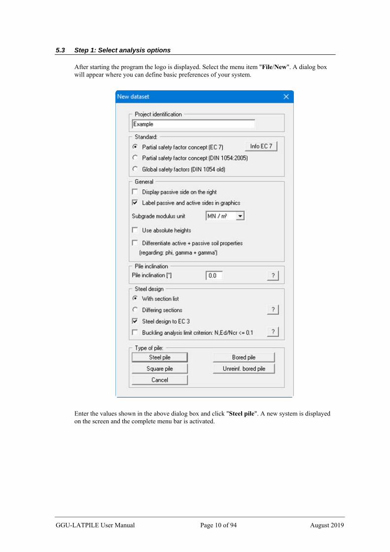
5.3 Step 1: Select analysis options

After starting the program the logo is displayed. Select the menu item "File/New". A dialog box will appear where you can define basic preferences of your system.

Enter the values shown in the above dialog box and click "Steel pile". A new system is displayed on the screen and the complete menu bar is activated.


5.4 Step 2: Enter system data

Go to the menu item "Editor 1/ System input" and enter the data for the pile head loading.

The pile width is required for determination of the spatial passive earth pressure. Using this menu item you also enter any groundwater level and distributed loads (see Section 7.2.2).


5.5 Step 3: Define berm on the active side

Go to the "Editor 1" menu and select "Berms (active side)":

Click "0 berm(s) to edit" and enter 1 as the new number of berms. Enter the following values and click "Done".

5.6 Step 4: Define berm on the passive side

Go to the "Editor 1" menu and select "Berms (passive side)". Click "0 berm(s) to edit" and enter the number 1. Enter the following values and click "Done".


5.7 Step 5: Define soils

Go to the "Editor 1" menu and select "Soils". Click the "Edit no. of soils" button and enter 3 as new number of soils. Enter the values shown in the following dialog box:


5.8 Step 6: Define type of earth pressure

Go to the "Editor 1" menu and select "Type of earth pressure".

The necessary buttons are already selected, so you need not change anything. The same applies to the remaining menu items in "Editor 1". However, you should click on these items and take a look at them, in order to familiarise yourself with them.


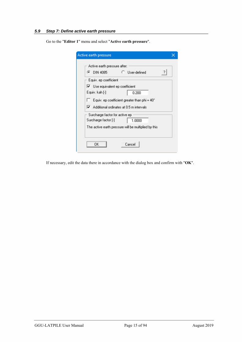
5.9 Step 7: Define active earth pressure

Go to the "Editor 1" menu and select "Active earth pressure".

If necessary, edit the data there in accordance with the dialog box and confirm with "OK".


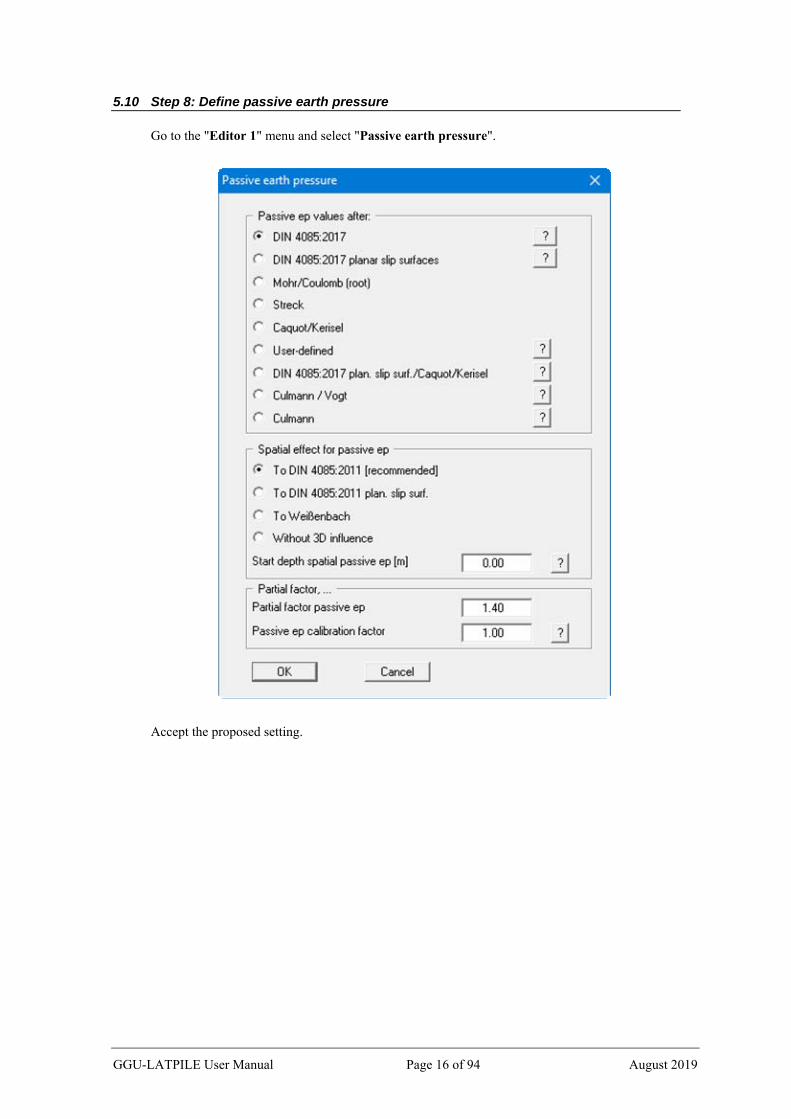
5.10 Step 8: Define passive earth pressure

Go to the "Editor 1" menu and select "Passive earth pressure".

Accept the proposed setting.


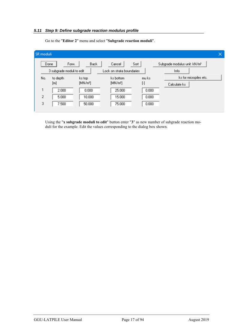
5.11 Step 9: Define subgrade reaction modulus profile

Go to the "Editor 2" menu and select "Subgrade reaction moduli".

Using the "x subgrade moduli to edit" button enter "3" as new number of subgrade reaction mo-duli for the example. Edit the values corresponding to the dialog box shown.


5.12 Step 10: Analyse system

Go to the "System" menu and select "Analyse".

The pile length and pile width were adopted from the "Editor 1/System input" dialog box. If you would prefer to use a different section, click the "Section: …" button and select the required sec-tion from the list of sections displayed. Confirm the input by pressing "OK".

EC 7 requires that a verification be performed to demonstrate that the soil stress (ks ꞏ w)d is smaller than the characteristic passive earth pressure eph,k (not reduced by a partial safety factor!). However, once analysis is complete it must be verified that the sum of the soil stress is smaller than the design passive earth pressure:

(ks ꞏ w)d ≤ Eph,k /Ep


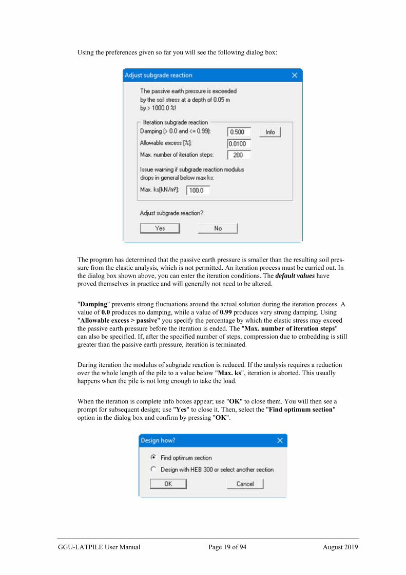
Using the preferences given so far you will see the following dialog box:

The program has determined that the passive earth pressure is smaller than the resulting soil pres-sure from the elastic analysis, which is not permitted. An iteration process must be carried out. In the dialog box shown above, you can enter the iteration conditions. The default values have proved themselves in practice and will generally not need to be altered.

"Damping" prevents strong fluctuations around the actual solution during the iteration process. A value of 0.0 produces no damping, while a value of 0.99 produces very strong damping. Using "Allowable excess > passive" you specify the percentage by which the elastic stress may exceed the passive earth pressure before the iteration is ended. The "Max. number of iteration steps" can also be specified. If, after the specified number of steps, compression due to embedding is still greater than the passive earth pressure, iteration is terminated.

During iteration the modulus of subgrade reaction is reduced. If the analysis requires a reduction over the whole length of the pile to a value below "Max. ks", iteration is aborted. This usually happens when the pile is not long enough to take the load.

When the iteration is complete info boxes appear; use "OK" to close them. You will then see a prompt for subsequent design; use "Yes" to close it. Then, select the "Find optimum section" option in the dialog box and confirm by pressing "OK".


You will then move directly to the design preferences dialog box (see menu item "System/Design defaults", Section 7.4.6).

Adopt the data and confirm by pressing "OK". An appropriate message box then opens. The set-tings given in the box for the optimum section can be adopted:


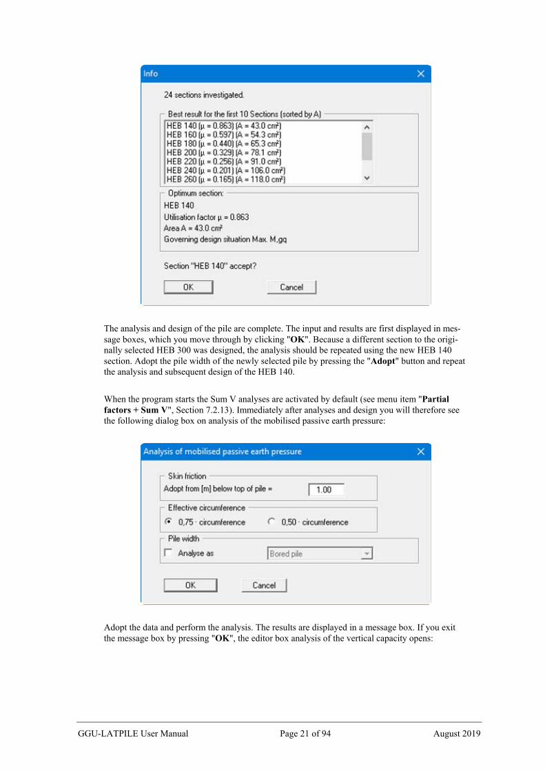
The analysis and design of the pile are complete. The input and results are first displayed in mes-sage boxes, which you move through by clicking "OK". Because a different section to the origi-nally selected HEB 300 was designed, the analysis should be repeated using the new HEB 140 section. Adopt the pile width of the newly selected pile by pressing the "Adopt" button and repeat the analysis and subsequent design of the HEB 140.

When the program starts the Sum V analyses are activated by default (see menu item "Partial factors + Sum V", Section 7.2.13). Immediately after analyses and design you will therefore see the following dialog box on analysis of the mobilised passive earth pressure:

Adopt the data and perform the analysis. The results are displayed in a message box. If you exit the message box by pressing "OK", the editor box analysis of the vertical capacity opens:


After accepting the settings by pressing "OK" the data are again displayed in a message box. By pressing the "Analyse again" button the above dialog box opens again and you can perform the analysis using the modified data.


5.13 Step 11: Evaluate and visualise the results

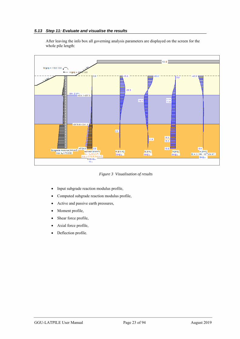
After leaving the info box all governing analysis parameters are displayed on the screen for the whole pile length:

Figure 3 Visualisation of results

Input subgrade reaction modulus profile,

Computed subgrade reaction modulus profile,

Active and passive earth pressures,

Moment profile,

Shear force profile,

Axial force profile,

Deflection profile.


The graphical visualisation, apart from showing the system, also contains other elements (referred to as legends) which contain further information and user input:

General legend This legend contains general information on the system.

Soil properties legend This legend contains data relating to the properties of every defined soil type.

Design legend This legend contains all data relating to design of steel sections or the cross-section of the analysed reinforced concrete pile.

Subgrade modulus legend The legend shows the specified subgrade reaction moduli along the pile section defined for the subgrade reaction modulus profile.

You can print the diagram on the printer (menu item "File/Print and export", Section 7.1.8), as well as a comprehensive table of data (menu item "File/Print output table", Section 7.1.5).

Using the program's zoom function, you can zoom in on selected sections of the graphics. If you double click with the left mouse button over a particular section of the graphics, the corresponding state variables will appear in an info box.

You can add further explanations or comments to the graphics using the Mini-CAD module. Save your work to data file by selecting "File/Save as" (Section 7.1.4).


6 Theoretical principles

6.1 General

GGU-LATPILE solves the differential equation for an elastically embedded pile using the given boundary conditions.

EJ ꞏ w'''' + kS ꞏ b ꞏ w = q

with

E = Young's modulus

J = moment of inertia

w = pile displacement

kS = subgrade reaction modulus

b = pile width

q = load

The solution is determined numerically using the so-called finite element method.

Action boundary conditions at the pile head can be defined (see menu item "Editor 1/System input"). At the pile toe, boundary conditions are generally:

Moment = 0.0;

Shear force = 0.0;

Vertical displacement = 0.0.

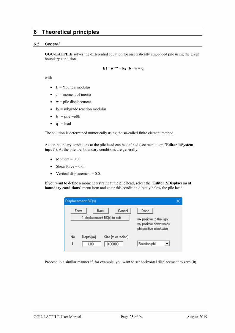
If you want to define a moment restraint at the pile head, select the "Editor 2/Displacement boundary conditions" menu item and enter this condition directly below the pile head:

Proceed in a similar manner if, for example, you want to set horizontal displacement to zero (0).


6.2 Soil properties

A maximum of 50 soil layers can be taken into consideration. The following parameters must be given for each:

depth in m below pile head, or absolute depth;

unit weight [kN/m³] of the moist soil ;

unit weight [kN/m³] of buoyant soil ' ;

friction angle [°];

cohesion (active and passive) [kN/m²];

active angle of wall friction as ratio of a/ ;

passive wall friction angle p/ ;

cone resistance from CPT qc or cone resistance qb,k,

shear strength of the undrained soil cu,k or skin friction qs,k.

If you activate the "Differentiate active + passive soil properties" check box in the dialog box in "File/New" or "Editor 1/Analysis options", you can enter differing friction angles and unit weights for the active and the passive sides.

To analyse the vertical capacity to EAU, EAB and EAP, enter the cone resistance qc and the shear strength of the undrained soil cu,k. When using empirical data, enter the values for qb,k and qs,k instead of qc and cu,k.

6.3 Active earth pressure

Active earth pressure is analysed to DIN 4085. DIN 4085 provides two relationships for the coefficients of earth pressure kah (friction) and kch (cohesion). Alternatively, there is the option of determining the cohesion coefficient from kch = kah

-2, a method often found in older literature.

6.4 At-rest earth pressure

The coefficient of at-rest earth pressure, k0 , is obtained after FRANKE (Die Bautechnik 1974/No. 1) from:

k0 = 1.0 - sin + (cos + sin - 1.0) ꞏ /

= wall friction angle = ground inclination

The vertical load component resulting from wall friction is obtained from the tangent of the angle of wall friction. However, in accordance with the EAB, a minimum value of 0.5 ꞏ the horizontal component is assumed when the tangent of the angle of wall friction is < 0.5.


6.5 Increased active earth pressure

The coefficient of increased active earth pressure, keh , is obtained from the coefficients of active earth pressure and at-rest earth pressure:

keh = (1.0 - f) ꞏ kah + f ꞏ k0

0.0 f 1.0

6.6 Passive earth pressure

The coefficient of passive earth pressure can be analysed using a number of methods:

DIN 4085:2017;

DIN 4085:2017 planar slip surfaces;

Streck,

Caquot/Kerisel,:p;

DIN 4085:2017 planar slip surfaces/ Caquot/Kerisel,

Culmann / Vogt,

Culmann.

The earth pressure after Culmann is acquired by varying the slip surface angle (see (sheet wall) Piling Handbook 1977). The forces at the earth pressure wedge are calculated using a slice method.

Following a proposal by Vogt (Dr. N. Vogt, Vorschlag für die Bemessung der Gründung von Lärmschutzwänden (Proposal for designing the footings of noise abatement walls), Geotechnik 1988, p. 210) a failure system corresponding to the pile width is considered. The friction and co-hesion forces acting on both sides of the failure system are incorporated in the calculation after Culmann. This determines a spatial passive earth pressure.

Otherwise, the following options are available for the spatial effect of the passive earth pressure:

To DIN 4085:2011;

To DIN 4085:2011 planar slip surfaces;

To Weißenbach;

Without 3D influence.


6.7 Berms

GGU-LATPILE can handle 10 berms on both the active and the passive sides. The berms can include surcharges. The effect on earth pressure is taken into consideration according to the Piling Handbook (Krupp Hoesch Stahl).

Figure 4 Berms on the active side

The following relationships apply for the parameters x and y:

x = kah0 / (kah - kah0) ꞏ a

y = kah0 / (kah - kah0) ꞏ x

eahu = ꞏ dh + surcharge

= unit weight of soil in the berm area

If the angle is greater than , it is assumed that = for analysis. Berms on the passive side are dealt with in exactly the same manner.



6.8 Area loads

Up to 10 area loads can be positioned on the active side at any height.

Possible types of earthpressure distribution

Type

Area load

eaho = 3 * eahu

Figure 5 Area load

The slip surface angle for the active earth pressure resulting from the self-weight of the soil is adopted for analysis compliant to DIN 4085.

a

a

ag

cossin

cossinsin

cosarctan

When there are a number of soil layers, GGU-LATPILE moves from layer to layer applying the appropriate angles of friction. The type of resulting earth pressure distribution can be defined in 4 different ways.

For at-rest pressure, the effects on the pile from area loads are determined using the theory of elastic half-space. The two load concentration factors "3" and "4" can be taken into consideration (also see Figure 6).

For over consolidated, cohesive soils use the concentration factor "3" applies, where: eop = q/ (2 - 1 + cos1 sin2 - cos2 sin2)

For cohesion less soils or non-over consolidated, cohesive soils use the concentration factor "4" applies, where: eop = q/4 (sin³2 - sin³1)

Area load

e op profile

Figure 6 At-rest earth pressure from area loads

With regard to the kind of earth pressure, area loads can be defined independent of the global preferences (see menu item "Editor 1/Type of earth pressure", Section 7.2.6).

6.9 Line loads

Line loads perpendicular to the pile axis are treated as shown in Fig. 4.20 on page 64 of the Piling Handbook 1977 (Spundwand-Handbuch). Data is entered in the form of a number of discrete area loads.


6.10 Bounded surcharges (active side)

Up to 10 bounded surcharges can be positioned at any height on the active side.

HE

p

a

e = k ꞏ pah ah

Figure 7 Bounded surcharge (active side)

The earth pressure coefficient k is acquired from kah for active earth pressure and from k0 for at-rest earth pressure. If this option is activated, the resulting earth pressure is then redistributed.

If negative values are entered, e.g. in order to generate a double-bounded surcharge, the linear component between and may not be adopted.


6.11 Bounded surcharges (passive side)

Up to 10 bounded surcharges may be adopted at any height on the passive side. The passive earth pressure is computed as follows:

p =10.0

p

e = k ꞏ pph ph

Figure 8 Bounded surcharge (passive side)


6.12 2nd order theory

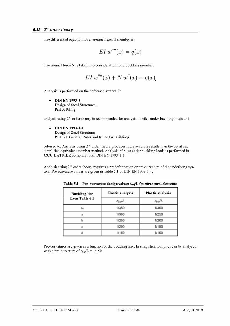
The differential equation for a normal flexural member is:

.

The normal force N is taken into consideration for a buckling member:

.

Analysis is performed on the deformed system. In

DIN EN 1993-5 Design of Steel Structures, Part 5: Piling

analysis using 2nd order theory is recommended for analysis of piles under buckling loads and

DIN EN 1993-1-1 Design of Steel Structures, Part 1-1: General Rules and Rules for Buildings

referred to. Analysis using 2nd order theory produces more accurate results than the usual and simplified equivalent member method. Analysis of piles under buckling loads is performed in GGU-LATPILE compliant with DIN EN 1993-1-1.

Analysis using 2nd order theory requires a predeformation or pre-curvature of the underlying sys-tem. Pre-curvature values are given in Table 5.1 of DIN EN 1993-1-1.

Pre-curvatures are given as a function of the buckling line. In simplification, piles can be analysed with a pre-curvature of e0,d/L = 1/150.


Using embedded piles without additional displacement boundary conditions the deformed system is defined by an inclination of the pile.

L

e0,d

Figure 9 Embedded pile

Using embedded piles with a horizontal displacement boundary condition (wx = 0), the deformed system is defined by a linear pre-curvature from the support point to the top of the pile and a para-bolic pre-curvature between the support points and the foot of the pile.

e0,d / 2

e0,d

linear

Parabel

Figure 10 Pile with a displacement boundary condition (wx = 0)


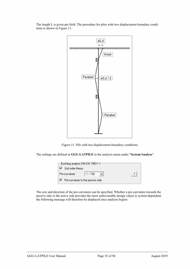
The length L is given per field. The procedure for piles with two displacement boundary condi-tions is shown in Figure 11.

e0,d / 2

e0,d

linear

Parabel

Parabel

Figure 11 Pile with two displacement boundary conditions

The settings are defined in GGU-LATPILE in the analysis menu under "System/Analyse".

The size and direction of the pre-curvature can be specified. Whether a pre-curvature towards the passive side or the active side provides the more unfavourable design values is system-dependent: the following message will therefore be displayed once analysis begins:


You must therefore deactivate the "Pre-curvature to passive side" check box following success-ful analysis and check, in a new analysis, whether pre-curvature to the active side delivers less favourable values.

In an analysis using 2nd order theory the necessary iteration process in terms of displacement is carried out using the design normal force Nd.

Subsequent design is based on a comparison of stresses

σd ≤ fy,k / γM = fy,k / 1,1 = fy,d

The "Example" folder contains 4 GGU-LATPILE files, which deal with the classical Euler cases 1 to 4. If the vertical load V at the pile head is increased slightly using the "Editor 1/System in-put" menu item and the system analysed, the following error message appears:

The normal force given in the data files thus corresponds to the buckling force determined after Euler.

6.13 Analysis of mobilised passive earth pressure

Detailed notes on this analysis concept are included in EAU 2012, Section 8.2.5.5, and in the Recommendations on Piling (2012).

6.14 Analysis of vertical capacity

Detailed notes on this analysis concept are included in EAU 2012, Section 8.2.5.5, and in the Recommendations on Piling (2012).


7 Description of menu items

7.1 File menu

7.1.1 "New" menu item

You can enter a new system using this menu item. You will see the following dialog box:

You can enter a dataset description ("Project identification") of the problem going to process, which will then be used in the General legend (see Section 7.6.7)

In the next group box the radio buttons are used to specify which safety concept to use for analysis and design.


Additionally, excavation visualisation to the right can be activated, as well as selecting kN/m³ or MN/m³ as the units for the modulus of subgrade reaction via a drop-down menu. The units can also be modified directly in the "Editor 2/Subgrade reaction moduli" menu item dialog box (see Section 7.3.1). If the "Label passive and active sides in graphics" check box is activated, both sides are labelled at the bottom of the system.

If you select the "Use absolute heights" check box you can enter all depths or heights in m AD (heights are positive upwards). If you leave this box unselected, the pile head is assumed at 0.0 (height/depth) and all input of layer depths etc. is positive downwards. Thanks to WYSIWYG there is no danger of using incorrect data, since all input is immediately visible on the screen. In this example and the following explanations of this manual the check box "Use absolute heights" is not selected.

If your system uses differing soil properties on the active and the passive sides, activate the "Differentiate active + passive soil properties" check box in the above dialog box. You will then be presented with different input columns for entering the active and passive friction angle and unit weight soil properties in the "Editor 1/Soils" menu item (Section 7.2.5). For better visualisation you can define the soil colours on the active and the passive sides differently using the Soil properties legend (see Section 7.6.8).

Below this, a pile inclination between -6° and +6° can be defined. Please read the information displayed after pressing the "?" button.

In the "Steel design:" group box, you can choose whether a section from the section list loaded by the program should be selected to design a steel pile, or whether you wish to design a steel pile with differing sections. If you work with the section list, the search for the optimum section in the list is performed automatically. The section list is loaded automatically when the program starts. However, you can expand and edit this list to suit your requirements (see Section 7.3.7). Steel design should always follow EC 3.

The type of pile to be analysed is specified using the buttons in the lower group box. If you decide to use a different pile type in the course of a project, simply select the menu item "File/New" and switch to the new pile type. Previously entered system data is retained!

If you select "Bored pile", subsequent design to EC 2 will assume a circular cross-section. If you select "Square pile", subsequent design to EC 2 will assume a square cross-section. The informa-tion with regard to "From section list" is irrelevant for "Bored pile", "Unreinf. bored pile" and "Square pile".

If you have changed to partial safety factor concept in the uppermost group box, you will see a further dialog box for specifying the partial factors after clicking the required pile type. Using the "Default values" button, you can accept the partial factors given in DIN 1054:2010 or EC 7 for the different load cases. The partial factors entered can be edited at any time using the "Edi-tor 1/Partial factors + Sum V" menu item (see Section 7.2.13).


7.1.2 "Load" menu item

You can load a file with system data, which was created and saved at a previous sitting, and then edit the data.

7.1.3 "Save" menu item

You can save data entered or edited during program use to a file, in order to have them available at a later date, or to archive them. The data is saved without prompting with the name of the current file. Loading again later creates exactly the same presentation as was present at the time of saving.

7.1.4 "Save as" menu item

You can save data entered during program use to an existing file or to a new file, i.e. using a new file name. For reasons of clarity, it makes sense to use ".p20" as file suffix, as this is the suffix used in the file requester box for the menu item "File/Load". If you choose not to enter an exten-sion when saving, ".p20" will be used automatically. If the current system has been analysed at the time of saving, the analysis results are saved in the file.

7.1.5 "Print output table" menu item

7.1.5.1 Selecting the output format

You can have a table printed containing the current analysis results. The results can be sent to the printer or to a file (e.g. for further editing in a word processor). The output contains all informa-tion on the current state of analysis, including the system data.

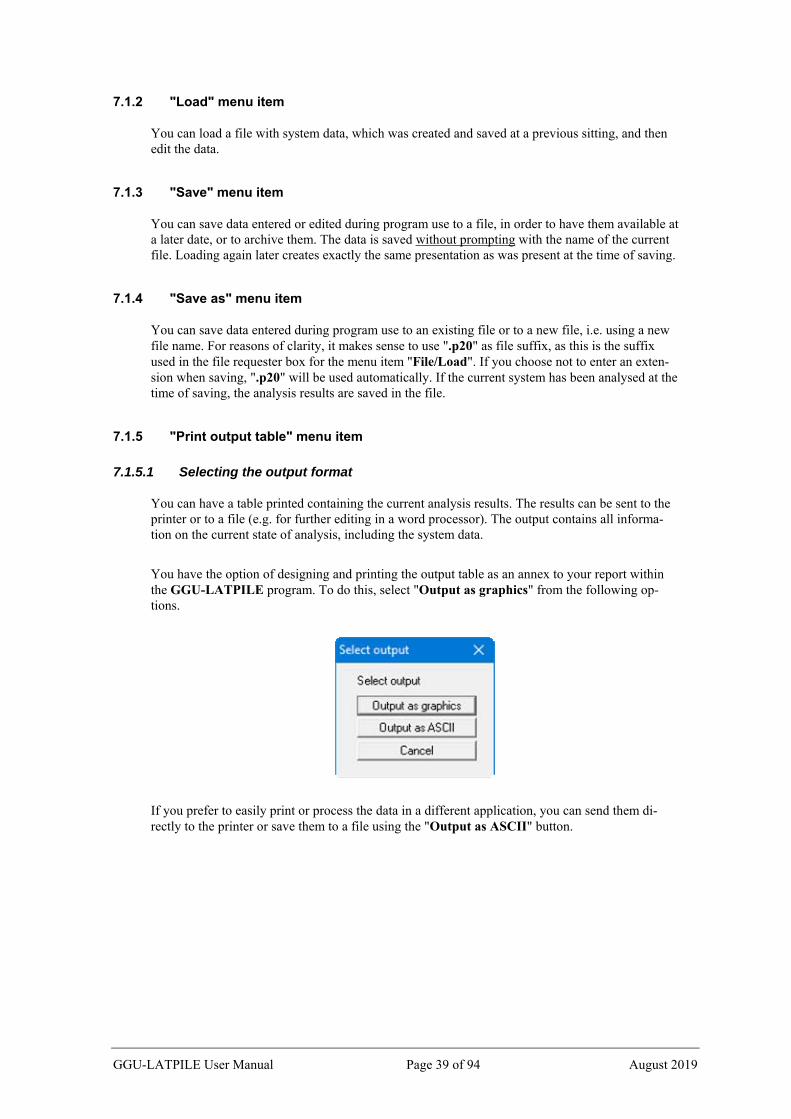
You have the option of designing and printing the output table as an annex to your report within the GGU-LATPILE program. To do this, select "Output as graphics" from the following op-tions.

If you prefer to easily print or process the data in a different application, you can send them di-rectly to the printer or save them to a file using the "Output as ASCII" button.


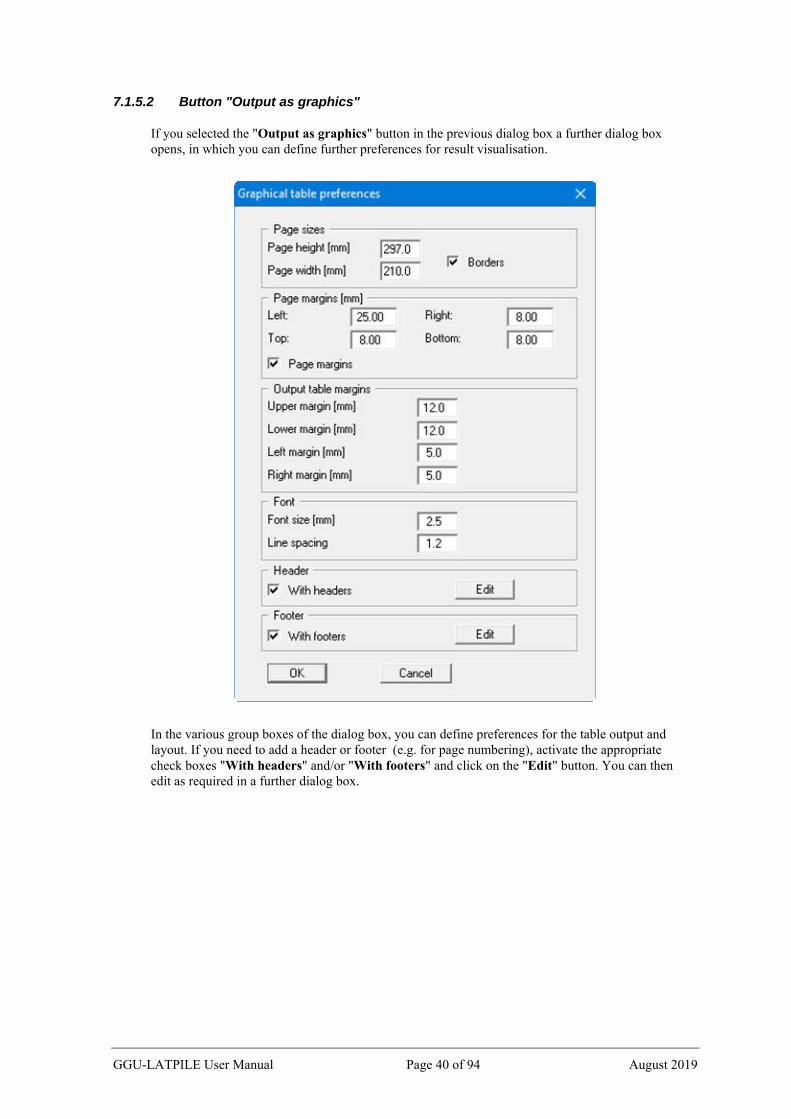
7.1.5.2 Button "Output as graphics"

If you selected the "Output as graphics" button in the previous dialog box a further dialog box opens, in which you can define further preferences for result visualisation.

In the various group boxes of the dialog box, you can define preferences for the table output and layout. If you need to add a header or footer (e.g. for page numbering), activate the appropriate check boxes "With headers" and/or "With footers" and click on the "Edit" button. You can then edit as required in a further dialog box.


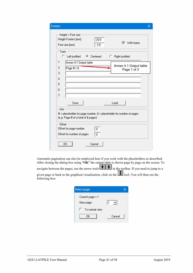
Automatic pagination can also be employed here if you work with the placeholders as described. After closing the dialog box using "OK" the output table is shown page by page on the screen. To

navigate between the pages, use the arrow tools in the toolbar. If you need to jump to a

given page or back to the graphical visualisation, click on the tool. You will then see the following box:

Annex 4.1 Output table Page 1 of 3


7.1.5.3 Button "Output as ASCII"

You can have your analysis data sent to the printer, without further work on the layout, or save it to a file for further processing using a different program, e.g. a word processing application.

In the dialog box you can define output preferences.

"Output preferences" group box Using the "Edit" button the current output preferences can be changed or a different printer selected. Using the "Save" button, all preferences from this dialog box can be saved to a file in order to have them available for a later session. If you select "GGU-LATPILE.drk" as file name and save the file in the program folder (default), the file will be automatically loaded the next time you start the program.

Using the "Page format" button you can define, amongst other things, the size of the left margin and the number of lines per page. The "Header/footer" button allows you to enter a header and footer text for each page. If the "#" symbol appears within the text, the current page number will be entered during printing (e.g. "Page #"). The text size is given in "Pts". You can also change between "Portrait" and "Landscape" formats.

"Print pages" group box If you do not wish pagination to begin with "1" you can add an offset number to the check box. This offset will be added to the current page number. The output range is defined us-ing "From page no." "to page no.".

"Output to:" group box Start output by clicking on "Printer" or "File". The file name can then be selected from or entered into the box. If you select the "Window" button the results are sent to a separate window. Further text editing options are available in this window, as well as loading, sav-ing and printing.


7.1.6 "Export" menu item

The general stability can be simply verified by exporting the data from GGU-LATPILE to GGU-STABILITY (GGU slope stability application). After clicking this menu item an appropriate file (".boe") can be generated with the required GGU-STABILITY version status.

7.1.7 "Output preferences" menu item

You can edit output preferences (e.g. swap between portrait and landscape) or change the printer in accordance with WINDOWS conventions.

7.1.8 "Print and export" menu item

You can select your output format in a dialog box. You have the following options:

"Printer" allows graphic output of the current screen contents (graphical representation) to the WINDOWS default printer or to any other printer selected using the menu item "File/Output preferences". But you may also select a different printer in the following dialog box by pressing the "Output prefs./change printer" button.

In the upper group box, the maximum dimensions which the printer can accept are given. Below this, the dimensions of the image to be printed are given. If the image is larger than the output format of the printer, the image will be printed to several pages (in the above ex-ample, 4). In order to facilitate better re-connection of the images, the possibility of enter-ing an overlap for each page, in x and y direction, is given. Alternatively, you also have the possibility of selecting a smaller zoom factor, ensuring output to one page ("Fit to page" button). Following this, you can enlarge to the original format on a copying machine, to en-sure true scaling. Furthermore, you may enter the number of copies to be printed.


If you have activated the table representation on the screen, you will see a different dialog box for output by means of the "File/Print and export" menu item button "Printer".

Here, you can select the table pages to be printed. In order to achieve output with a zoom factor of 1 (button "Fit in automatically" is deactivated), you must adjust the page format to suit the size format of the output device. To do this, use the dialog box in "File/Print output table" button "Output as graphics".

"DXF file" allows output of the graphics to a DXF file. DXF is a common file format for transferring graphics between a variety of applications.

"GGU-CAD file" allows output of the graphics to a file, in order to enable further processing with the GGU-CAD program. Compared to output as a DXF file this has the advantage that no loss of colour quality occurs during export.

"Clipboard" The graphics are copied to the WINDOWS clipboard. From there, they can be imported into other WINDOWS programs for further processing, e.g. into a word processor. In order to import into any other WINDOWS program you must generally use the "Edit/Paste" function of the respective application.

"Metafile" allows output of the graphics to a file in order to be further processed with third party soft-ware. Output is in the standardised EMF format (Enhanced Metafile format). Use of the Metafile format guarantees the best possible quality when transferring graphics.

If you select the "Copy/print area" tool from the toolbar, you can copy parts of the graphics to the clipboard or save them to an EMF file. Alternatively you can send the marked area directly to your printer (see "Tips and tricks", Section 8.4). Using the "Mini-CAD" program module you can also import EMF files generated us-ing other GGU applications into your graphics.


"Mini-CAD" allows export of the graphics to a file in order to enable importing to different GGU appli-cations with the Mini-CAD module.

If the "Retain Mini-CAD layers" check box is activated, the layer allocations for any ex-isting Mini-CAD elements are saved. Otherwise, all Mini-CAD elements are saved on Layer 1 and are also inserted into Layer 1 in other GGU programs via the "Load" function in the Mini-CAD pop-up menu.

By activating the "Output global coordinates" check box, the present graphics are saved in the system coordinates [m]. Otherwise they are saved in the page coordinates [mm]. If you import the Mini-CAD file saved using "Global coordinates" into a different GGU program, the coordinates are also transferred. If a system is transferred from GGU-STABILITY to GGU-2D-SSFLOW, for example, the system coordinates and scale are corrected compliant with the transferred global coordinates, after importing the file and pressing the function key [F9] (menu item "Page size + margins/Auto-resize").

"GGUMiniCAD" allows export of the graphics to a file in order to enable processing in the GGUMiniCAD program.

"Cancel" Printing is cancelled.


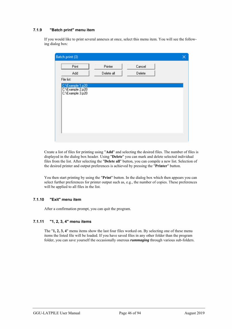
7.1.9 "Batch print" menu item

If you would like to print several annexes at once, select this menu item. You will see the follow-ing dialog box:

Create a list of files for printing using "Add" and selecting the desired files. The number of files is displayed in the dialog box header. Using "Delete" you can mark and delete selected individual files from the list. After selecting the "Delete all" button, you can compile a new list. Selection of the desired printer and output preferences is achieved by pressing the "Printer" button.

You then start printing by using the "Print" button. In the dialog box which then appears you can select further preferences for printer output such as, e.g., the number of copies. These preferences will be applied to all files in the list.

7.1.10 "Exit" menu item

After a confirmation prompt, you can quit the program.

7.1.11 "1, 2, 3, 4" menu items

The "1, 2, 3, 4" menu items show the last four files worked on. By selecting one of these menu items the listed file will be loaded. If you have saved files in any other folder than the program folder, you can save yourself the occasionally onerous rummaging through various sub-folders.


7.2 Editor 1 menu

7.2.1 "Analysis options" menu item

Using this menu item you can edit the default preferences of the current system. The dialog box corresponds to the box in the menu item "File/New" (see description in Section 7.1.1).

7.2.2 "System input" menu item

Enter the forces at the pile head for the pile you have used into a dialog box, as well as further system parameters.

You see the above dialog box if you have selected the partial safety factors in "File/New" or "Editor 1/Analysis options" menu items. The permanent and changeable loads are entered sepa-rately in accordance with the partial safety factor concept. You define both the pile length and the pile width. The width is required for determination of the spatial passive earth pressure.

The loads specified in M EBGS-Lsw 2018 can be determined for analysis of piles for noise abate-ment walls. In the dialog box that opens after clicking the respective button, select the required data. A dynamic wind loading factor can be defined.

If you checked the "Use absolute heights" box when defining the system, an additional entry, "Top of pile", appears in the dialog box for specifying the absolute position. In this case, all heights are measured in m AD or m site zero, i.e. the y-axis is positive upwards. You can then enter a value, for example, of 86.42 [m AD] in the "Top of pile" field. All further input must then be with reference to this value.


If the height of a previously defined system is subsequently set to absolute heights, a query fol-lows after leaving the dialog box above asking for confirmation of whether soil strata and defined elements such as area loads, for example, should be adapted to the new pile top. Adaptation would mean that the depth of a soil layer entered as a positive value would be converted from, for exam-ple, 7.5 m to an absolute height of -7.5 m AD. If then, you only convert your system to [m AD], do not select any elements in the query box and press the "OK" button.

In the lower group box, you can define the groundwater level and a distributed load. If you are working with the partial safety factors used in DIN 1054 (new), decide whether the distributed load is "Permanent", "Changeable" or the "Component above 10.0 kN/m² changeable" (see the following dialog box). "Component above 10.0 kN/m² changeable" means, for example, that for an input of 13.5 kN/m², 10 kN/m² are adopted as permanent and 3.5 kN/m² as changeable in the analysis.

7.2.3 "Berms (active side)" menu item

You can define a maximum of 10 berms on the active side.

Enter the x-ordinates of the toe and head of the berm. With "delta h" you define the height of the berm, whereby negative values are also permitted. Finally, a "Surcharge" on the horizontal sur-face behind the head of the berm can be entered.

If more than one berm is present in the system, click "x berm(s) to edit" and enter the number of berms.

Berms may not overlap. The program checks that this condition is adhered to and warns of any errors.

7.2.4 "Berms (passive side)" menu item

Berms on the passive side are defined in exactly the same manner as for the active side, but with-out the "Live load" check box.


7.2.5 "Soils" menu item

You can define the soil properties in the following dialog box. In stratified soils first the number of layers must be entered under "Edit no. of soils".

Using the "Common soils" button, you can easily select the soil properties of many common soils from a database or determine intermediate values. In the dialog box, which you open by pressing the "Common soils" button, open the "Soils_english.gng_ggu" file when first starting the pro-gram in English ("Edit table"/"Load" buttons). Then save the data set in the "Soils.gng_ggu" file on the program level in order to open your modified database file when the program starts. You can also enter your own data ("Edit table"/"x soils to edit" button) and save it in the "Soils.gng_ggu" file. You can also use your adapted file in other GGU programs by means of the "Common soils" function if you copy the file into the appropriate GGU program folder.

Layer depths (except when using the modulus of subgrade reaction) are always with reference to the top of the pile, or are in absolute values (m AD), if this was selected in the initial dialog box of the "File/New" menu item.

If you have activated the "Differentiate active + passive soil properties" check box in the dialog box in "File/New" or "Editor 1/Analysis options", you can enter differing friction angles and unit weights for the active and the passive sides.

To analyse the vertical capacity to EAU, EAB and EAP, enter the cone resistance qc and the shear strength of the undrained soil cu,k. When using empirical data, enter the values for qb,k and qs,k instead of qc and cu,k. To do this, activate the "Use own empirical data (not recommended)" check box in the "Editor 1/Partial factors + Sum V" menu item dialog box (see Section 7.2.13).

Clicking the "Sort" button sorts the soil layers according to depth; however, this is performed automatically when you click "OK" to leave the dialog box. This eliminates the possibility of input errors.


You can also use this function to eliminate a soil from the table. Simply assign the soil to be eliminated a greater layer depth and then click the "Sort" but-ton. The corresponding soil is now the last soil in the table and can be deleted by reducing the number of soils.

7.2.6 "Type of earth pressure" menu item

In this dialog box you define the type of earth pressure on which the analysis is to be based.

The options for area loads can be specified separately.


7.2.7 "Active earth pressure" menu item

You can specify active earth pressure preferences using this dialog box:

In the upper group box you specify the type of active earth pressure calculation. The other two methods are only of interest if you wish to analyse an example from older literature sources or check certain results.

The "Use equivalent ep coefficient" check box should only be deactivated in exceptional circum-stances (see EAB R 4). The equivalent earth pressure coefficient can only be smaller than 0.2 in special circumstances (see EAB R 4). It only makes sense to deactivate this check box when re-examining existing analyses (for instance, all the examples used in the Piling Handbook). Alterna-tively, the equivalent earth pressure coefficient can be defined by means of a friction angle phi = 40°. This procedure also takes the defined wall friction angle into consideration.

A number of applications on the market also provide the option of a general increase in active earth pressure, apart from certain forms or earth pressure redistribution. In order to be able to check analysis performed with such an application, GGU-LATPILE also offers the possibility.


7.2.8 "Passive earth pressure" menu item

You can specify passive earth pressure preferences using this dialog box:

In the upper group box you specify the type of passive earth pressure calculation (see also Section 6.6).

The spatial effect of the passive earth pressure can be set to the mid-region.

If you have selected partial safety factors, enter the partial factor for passive earth pressure and the calibration factor in the dialog box in accordance with the information in DIN 1054:2010/EC 7.


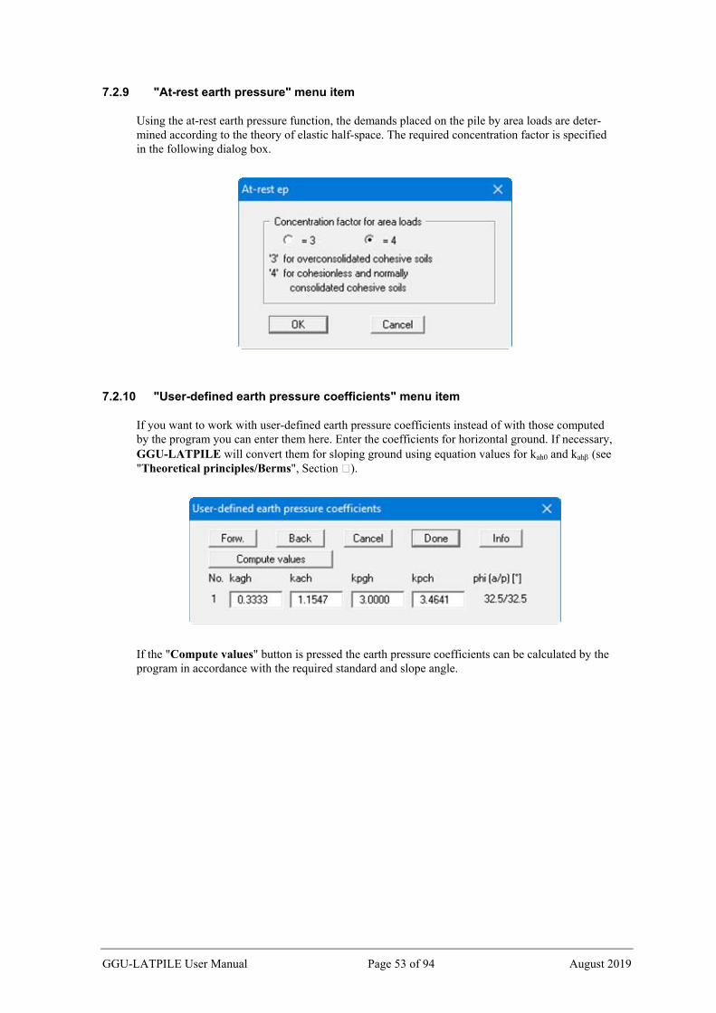
7.2.9 "At-rest earth pressure" menu item

Using the at-rest earth pressure function, the demands placed on the pile by area loads are deter-mined according to the theory of elastic half-space. The required concentration factor is specified in the following dialog box.

7.2.10 "User-defined earth pressure coefficients" menu item

If you want to work with user-defined earth pressure coefficients instead of with those computed by the program you can enter them here. Enter the coefficients for horizontal ground. If necessary, GGU-LATPILE will convert them for sloping ground using equation values for kah0 and kah (see "Theoretical principles/Berms", Section ).

If the "Compute values" button is pressed the earth pressure coefficients can be calculated by the program in accordance with the required standard and slope angle.


7.2.11 "Seismic acceleration" menu item

Seismic loads can be taken into consideration as described in EC 8 or EAU 1990, Section 2.14, by increasing the active earth pressure coefficients and reducing the passive earth pressure coeffi-cients. Seismic loads are given in multiples of gravitational acceleration (g).


7.2.12 "Analysis of Sum V" menu item

If you are analysing with the global safety factor concept to DIN 1054 (old), you can activate the analysis of mobilised passive earth pressure using this menu item.

If the check box is activated, the dialog box allowing selection of the analysis options for the mo-bilised passive earth pressure opens immediately following your analysis and design.

If the system has already been analysed the modifications required for analysis of mobilised pas-sive earth pressure can be more easily made using the menu item "Evaluation/Sum V analyses", because the system then need not be analysed once again (see Section 7.5.3).


7.2.13 "Partial factors + Sum V" menu item

If you are analysing with the partial safety factor concept, you will see a dialog box for defining the partial factors.

In the dialog box's lower group box, activate required Sum V analyses using the two check boxes. When the check boxes are activated analysis is performed automatically following your system analysis and design (see the example in Section 5.12).

On a previously analysed system, you can perform the analyses with a variety of settings via the menu item "Evaluation/Sum V analyses" (see Section 7.5.3), without having to reanalyse the system.

In the "Default values" group box the partial factors for the various load cases and subsoil condi-tions given in the DIN 1054:2010 and in the EC 7 can be selected by means of the dialog box reached by clicking the "To DIN 1054:2010" button. The selected design situation is automati-cally entered at the top of the dialog box and shown later in the General legend. However, you can also use your own designations. The load case designations were altered for the EC 7 partial safety factor concept:

Load Case 1 is now DS-P: Persistent Design Situation

Load Case 2 is now DS-T: Transient Design Situation

Load Case 3 is now DS-A: Accidental Design Situation

In addition, there is a seismic design situation (DS-E). In the DS-E design situation all partial factors = '1.0'. It is also possible to select the partial safety factors compliant with Austrian stan-dards using the "To ÖNORM EN 1997-1" button.


7.3 Editor 2 menu

7.3.1 "Subgrade reaction moduli" menu item

As the analysis is to be performed for an elastically embedded pile toe, it is necessary to enter a modulus of subgrade reaction. In this dialog box you can enter the profile of the subgrade reaction moduli.

The number of subgrade reaction moduli can be adapted to your system using the "x subgrade moduli to edit" button.

In the field designated "mu ks" the tangential bedding is given as a multiple of the horizontal bedding. However, the factor is generally of little importance, since the pile toe is considered to be vertically non-displaceable, meaning that deformations in a longitudinal direction, and any associ-ated tangential subgrade reaction moduli, are small.

The units can be changed from MN/m³ to kN/m³ and vice versa using the "Subgrade reaction modulus unit: kN/m³" check box.


7.3.2 "Displacement boundary conditions" menu item

You can introduce additional displacement boundary conditions anywhere along the pile.

In the above example, a rotation phi of 0.0 has been entered 2.0 m below the top of the pile. Alter-natively to "Rotation phi" you can select "Displ. wx" or " Displ. wy", which stand for horizontal and vertical displacement respectively.

7.3.3 "Action boundary conditions" menu item

You can introduce additional action boundary conditions anywhere along the pile.

The direction of the forces is defined by means of the sign. In the example above a horizontal force of 15 kN/m has been entered at the top of the pile, acting towards the left.


7.3.4 "Lateral pressures" menu item

If, in addition to the diverse possibilities for determining earth pressure on the pile, you also need to take additional surcharges on the active side into consideration, this is where to enter them.

The number of lateral pressures can be modified using the "x lateral pressure(s) to edit" button. Then enter the ordinates in metres from the top of the pile or as absolute heights, and the values for the lateral pressures.

7.3.5 "Area and line loads" menu item

Using this menu item you define area loads and line loads.

The "x area load(s) to edit" button allows you to determine the number of area loads to be con-sidered. Subsequently you can enter the sizes "p(v)" (= vertical) and "p(h)" (= horizontal), the ordinates and the "Depth" of the area loads. You must also enter the "Type" (shape) of the resul-tant horizontal forces on the pile (see also Section 6.8). For defining an area load as a live load, select the corresponding check box on the right.

Using the "Generate line loads" button, line loads acting vertically on the pile may be considered adopted as area loads (see Section 6.9).


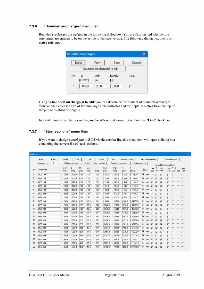
7.3.6 "Bounded surcharges" menu item

Bounded surcharges are defined in the following dialog box. You are first queried whether the surcharges are entered to be on the active or the passive side. The following dialog box opens for active side input:

Using "x bounded surcharge(s) to edit" you can determine the number of bounded surcharges. You can then enter the size of the surcharges, the ordinates and the depth in metres from the top of the pile or as absolute heights.

Input of bounded surcharges on the passive side is analogous, but without the "Live" check box.

7.3.7 "Steel sections" menu item

If you want to design a steel pile to EC 3 via the section list, this menu item will open a dialog box containing the current list of steel sections.


The following options are available:

"Forw.", "Back", "Go to no." You can navigate through the list using "Forw." and "Back". "Go to no." allows you to jump to the section specified.

"Cancel", "Done" Exit the dialog box either saving or rejecting your modifications using these buttons.

"x Sections to edit", "Info" Using this button you may expand or reduce the list of steel sections. New sections are added to the end of the list. A description of the abbreviations used to enter the section data is available via the "Info" button.

"Load", "Save", "Sort", "Delete doubles" A different section list can be opened by pressing the "Load" button. It is then possible to append the new list to an already open section list. After appending sections it may be ex-pedient to delete any double sections in the list by pressing the "Delete doubles" button. The sections can then be sorted either by moment of inertia or by name by pressing the "Sort" button. The modified section list may then be saved to the program folder as ".tbw_ggu" file for subsequent analyses by pressing the "Save" button.

"Select section" A dialog box opens in which you select the required section for design.

"Simulate corrosion" You can define the corrosion for any sections, which is then used to calculate the new sec-tion data. The new section data can be allocated to the selected section, or to a different, ex-isting section. The data can also be allocated to a new section, which is added to the exist-ing list.

Corrosion in tubular sections can be generated using the "Create tubular section" button (see next side).

"Weld on plates" If you need to simulate reinforcement using weld-on plates, click the previous "Simulate corrosion" button and enter a negative corrosion.


"Create tubular section" A new tubular section can be generated. A dialog box opens for entering the dimensions and identification. In the following dialog box you can then save the section as a new sec-tion, or using a previously allocated name:

"Delete sections" Any number of sections in a sequence in the list can be deleted using this button.

"Create old record" Using this button you can save a record containing the old section tables based on the global safety factors (".tbw", ".spw").

If Steel design to EC 3 is not activated, the old dialog box opens. A check box in front of the number of each steel section can be activated. This is used to select the respective steel section. If you then press the "Selected section as design section" button, this section is used as the design section. The section parameters ("h" = height; "b" = width; "A" = area; "I" = moment of inertia) can be edited. The program uses I and h to determine the section modulus W during the subse-quent design phase. The variable S is the first moment of area of the section and s is the web thickness. The value of "S/s" is required for verification of shear stress.


7.3.8 "Differing sections" menu item

If you want to design a steel pile using differing sections at different depths, you can use this menu item to define the different individual sections for the pile. For example, this can be used to represent partial corrosion of the steel pile, as shown in the following dialog box:

First, define the required number of sections using the "x Different sections to edit" button. After clicking the button with the section designation you will see a dialog box in which you can select the required section from the section list. You can save your section compilation in a ".sol_ggu" file and load it again when needed using the "Load" and "Save" buttons. The sections are sorted according to depth using "Sort".

If you are working with differing sections, you specify the steel grade and buckling analysis for the individual sections in the dialog box for this menu item.

If you exit this menu item and have previously selected "With section list" in "Editor 1/Analysis options", you will be asked whether you wish to convert to steel design using differing sections. You will see a similar question if the case is vice versa. If you have already selected "Differing sections" and would like to add a section (e.g. with corrosion), you can go to the "Editor 2/Steel sections" and add the required section without having to immediately move back to "With section list" again. When you exit this menu item you will see the reverse question: whether to change to steel design using the section list. In this case, respond negatively and supplement your new sec-tion using the menu item "Editor 2/Differing sections".

7.3.9 "Young's modulus/Specific weight" or "Specific weight" menu items

This menu item has two separate designations and opens two different dialog boxes depending on whether you are working with a section list or with user-defined section data:

"Young's modulus/Specific weight" When working with the section list, you must enter Young's modulus and specific weight of the pile. From the former the bending line is calculated, from the latter the self-weight of the pile.

"Specific weight" Using differing sections Young's modulus is entered in the corresponding dialog box, so that here it is only necessary to specify the specific weight of the pile.


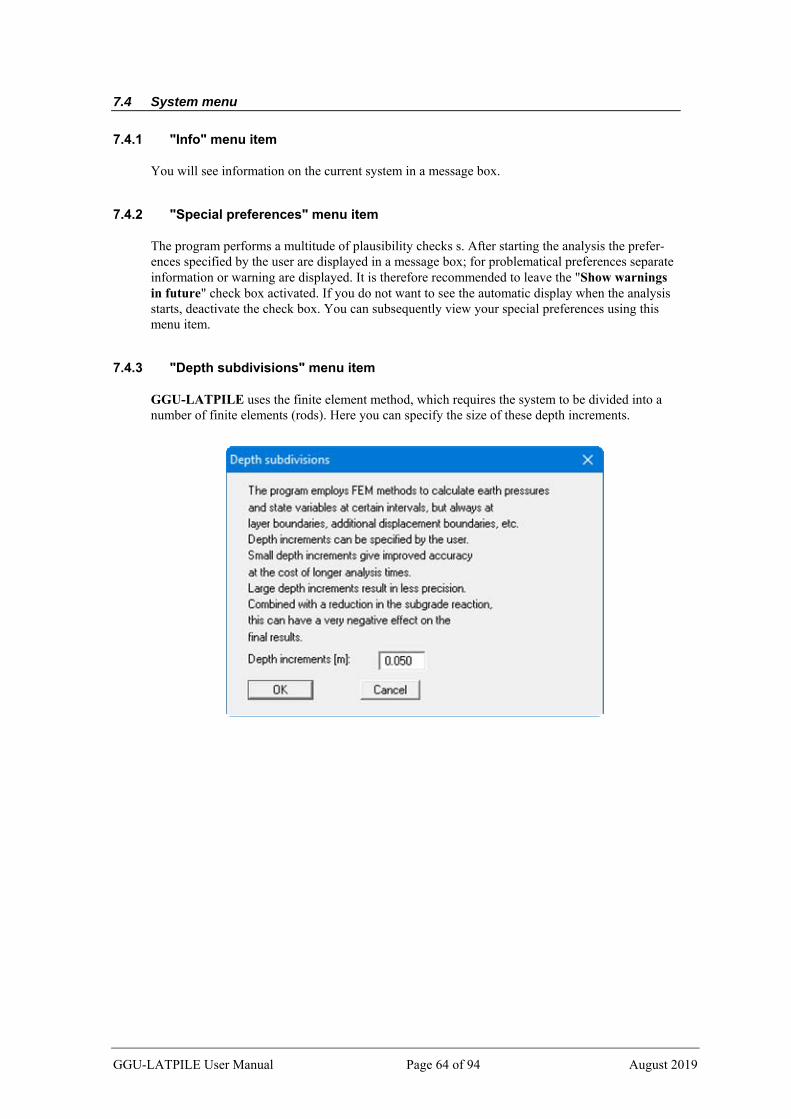
7.4 System menu

7.4.1 "Info" menu item

You will see information on the current system in a message box.

7.4.2 "Special preferences" menu item

The program performs a multitude of plausibility checks s. After starting the analysis the prefer-ences specified by the user are displayed in a message box; for problematical preferences separate information or warning are displayed. It is therefore recommended to leave the "Show warnings in future" check box activated. If you do not want to see the automatic display when the analysis starts, deactivate the check box. You can subsequently view your special preferences using this menu item.

7.4.3 "Depth subdivisions" menu item

GGU-LATPILE uses the finite element method, which requires the system to be divided into a number of finite elements (rods). Here you can specify the size of these depth increments.


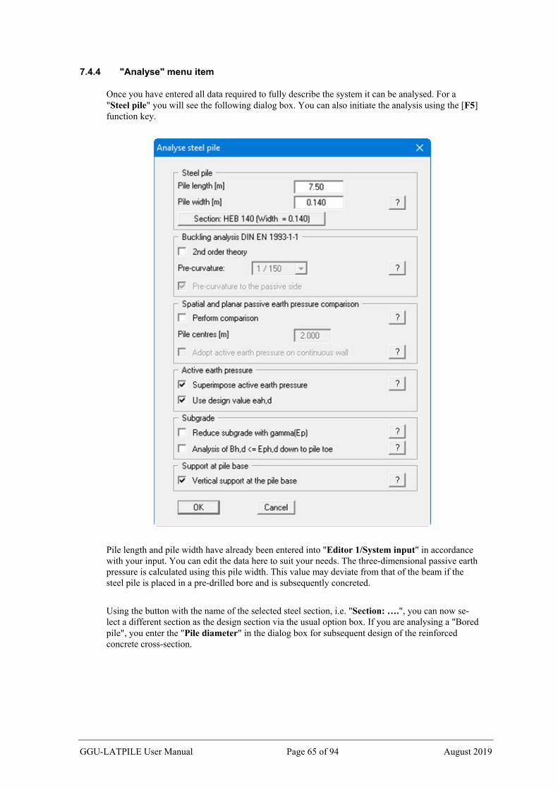
7.4.4 "Analyse" menu item

Once you have entered all data required to fully describe the system it can be analysed. For a "Steel pile" you will see the following dialog box. You can also initiate the analysis using the [F5] function key.

Pile length and pile width have already been entered into "Editor 1/System input" in accordance with your input. You can edit the data here to suit your needs. The three-dimensional passive earth pressure is calculated using this pile width. This value may deviate from that of the beam if the steel pile is placed in a pre-drilled bore and is subsequently concreted.

Using the button with the name of the selected steel section, i.e. "Section: ….", you can now se-lect a different section as the design section via the usual option box. If you are analysing a "Bored pile", you enter the "Pile diameter" in the dialog box for subsequent design of the reinforced concrete cross-section.


Piles subject to buckling hazards can be analysed using "2nd order theory". A system pre-curvature, which can be adopted at 1/150, must be defined for buckling analysis to DIN EN 1993-5 or DIN EN 1993-1-1. The direction of pre-curvature must also be defined (to the passive side or the active side). Whether a pre-curvature towards the passive side or the active side provides the more unfavourable design values is system-dependent: it is therefore absolutely vital that both directions are investigated in a buckling analysis (see "Theoretical principles/2nd order theory", Section 6.12).

EC 7 requires that a verification be performed to demonstrate that the soil stress (ks ꞏ w)d is smaller than the characteristic passive earth pressure eph,k (not reduced by a partial safety factor!). However, once analysis is complete it must be verified that the sum of the soil stress is smaller than the design passive earth pressure:

(ks ꞏ w)d ≤ Eph,k /Ep

If the check box is deactivated, Bh,d and Eph,d are only cumulated to the pile pivot.

In some systems, tensile forces can occur at the pile base.This is due to the vertical immovability of the wall toe generated by the program.In bedded systems this boundary condition can be deac-tivated.However, when adopting the subgrade reaction modulus definition it is necessary that a tangential subgrade with the factor "µ(ks)"<> 0.0 is defined.The resulting normal force at the pile base is then more realistic.The value of "µ(ks)" generally has no great influence on the analysis results.The "Vertical support at the pile base" check box should only be deactivated if tensile forces occur at the pile base when the check box is activated!

After leaving the dialog box with "OK", the program checks whether the passive earth pressure is smaller than the resulting soil pressure from the elastic analysis, which is not permitted. In this case you see a dialog box for adjusting the subgrade reaction (see further explanations in the worked example, Section 5.12).

Following the analysis you can immediately carry out the design after confirming at the prompt. You then move directly to a dialog box, which can also be reached via the "System/Design de-faults" menu item (see Section 7.4.6).


7.4.5 "Optimise" menu item

Using this function it is possible to optimise pile length. You can also initiate this function press-ing the [F7] function key.


In the top section of the dialog box you enter the minimum and maximum pile length, as well as a delta pile length, thereby defining the range of lengths from which the optimum length should be selected. For example, the values in the dialog box shown above will result in the lengths 6.00, 6.25, 6.50, 6.75,..., 8.00 m being investigated. The middle section of the dialog box relates to the iteration process. The default values have proved themselves in practice and will generally not need to be altered (see further explanations in the worked example, Section 5.12). In the bottom section of the dialog box, additional iteration criteria can be defined.

Once optimisation is complete, the optimum pile length can be transferred to your system. The system should then be reanalysed.

7.4.6 "Design defaults" menu item

Once the current system has been analysed you can progress directly to the pile design (see menu item "System/Analyse", Section 7.4.4). In addition, using this menu item, you can also carry out subsequent design for a different section to that used for the analysis.

When designing a steel pile the following dialog box opens containing two options for selecting the section:

You can search for the optimum section in the section list (see the example in Section 5.12). By activating the bottom option the analysis is performed using the previously selected design sec-tion. However, in the subsequent dialog box you can also select a different design section.


When design is complete you are informed of the verification results in an information box and are presented with the principal data on which the design was based. After confirming with "OK", the state variables and the system are presented on the screen.


7.4.7 "Graph positioning preferences" menu item

If you are not happy with the automatic graph arrangement you can arrange them to suit your needs using this menu item. First, activate the "Manual graph positioning" radio button.

The diagrams will then be shown central at the position "x" with the specified "Width".

The fastest way to modify the position of a graph is to press the [F11] function key and then to pull the graph to the new position holding the left mouse button pressed.


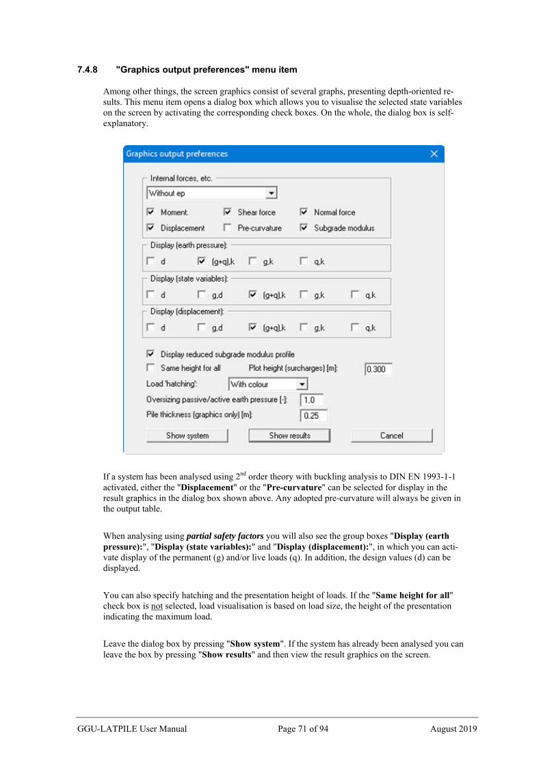
7.4.8 "Graphics output preferences" menu item

Among other things, the screen graphics consist of several graphs, presenting depth-oriented re-sults. This menu item opens a dialog box which allows you to visualise the selected state variables on the screen by activating the corresponding check boxes. On the whole, the dialog box is self-explanatory.

If a system has been analysed using 2nd order theory with buckling analysis to DIN EN 1993-1-1 activated, either the "Displacement" or the "Pre-curvature" can be selected for display in the result graphics in the dialog box shown above. Any adopted pre-curvature will always be given in the output table.

When analysing using partial safety factors you will also see the group boxes "Display (earth pressure):", "Display (state variables):" and "Display (displacement):", in which you can acti-vate display of the permanent (g) and/or live loads (q). In addition, the design values (d) can be displayed.

You can also specify hatching and the presentation height of loads. If the "Same height for all" check box is not selected, load visualisation is based on load size, the height of the presentation indicating the maximum load.

Leave the dialog box by pressing "Show system". If the system has already been analysed you can leave the box by pressing "Show results" and then view the result graphics on the screen.


7.4.9 "Labelling preferences" menu item

This menu item allows you to specify labelling preferences for the system visualisation and the result graphics.

In the dialog box, you activate the required check boxes and select the preferences for alignment or font sizes.

7.4.10 "Graph grid preferences" menu item

Here you can define graph grids for moments, shear forces and normal forces.


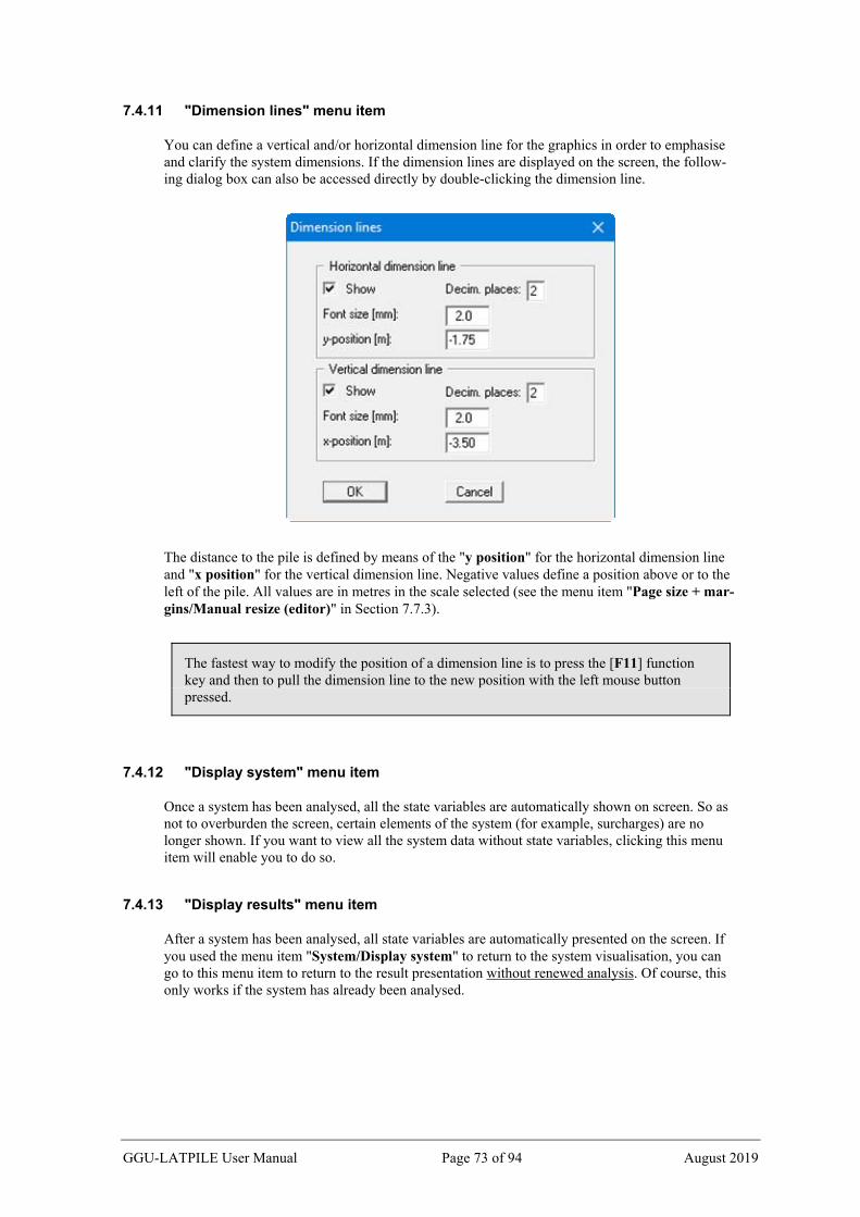
7.4.11 "Dimension lines" menu item

You can define a vertical and/or horizontal dimension line for the graphics in order to emphasise and clarify the system dimensions. If the dimension lines are displayed on the screen, the follow-ing dialog box can also be accessed directly by double-clicking the dimension line.

The distance to the pile is defined by means of the "y position" for the horizontal dimension line and "x position" for the vertical dimension line. Negative values define a position above or to the left of the pile. All values are in metres in the scale selected (see the menu item "Page size + mar-gins/Manual resize (editor)" in Section 7.7.3).

The fastest way to modify the position of a dimension line is to press the [F11] function key and then to pull the dimension line to the new position with the left mouse button pressed.

7.4.12 "Display system" menu item

Once a system has been analysed, all the state variables are automatically shown on screen. So as not to overburden the screen, certain elements of the system (for example, surcharges) are no longer shown. If you want to view all the system data without state variables, clicking this menu item will enable you to do so.

7.4.13 "Display results" menu item

After a system has been analysed, all state variables are automatically presented on the screen. If you used the menu item "System/Display system" to return to the system visualisation, you can go to this menu item to return to the result presentation without renewed analysis. Of course, this only works if the system has already been analysed.


7.5 Evaluation menu

7.5.1 "Main output summary" menu item

A message box appears containing the main system analysis parameters. This function can also be initialized pressing the [F6] function key.

You are also informed that double-clicking the left mouse button (after you have closed the mes-sage box) on any part of the graphics will cause the corresponding state variables to be shown on screen.

7.5.2 "Maximum reaction summary" menu item

You will see the maximum values for all state variables.

7.5.3 "Sum V analyses" menu item

Using this menu item it is possible to analyse Sum V once again for a previously analysed system. If analysis of Sum V was not previously activated, it is activated now via a prompt box. The acti-vation is then shown in the "Editor 1/Analysis of Sum V" or "Editor 1/Partial factors + Sum V" dialog boxes (see Sections 7.2.12 and 7.2.13).

The circumference is required for analysis of Sum V. Both rectangular steel sections (HEB) and circular, tubular sections may be adopted as steel sections. If the analysis is activated a dialog box opens allowing the steel cross-section to be selected.


In the subsequent dialog box the type of analysis or the effective circumference may be modified for the analysed system. This dialog box always opens immediately following analysis and design if analysis of Sum V is activated. For a bored pile analysis you can also specify whether the bored pile should be designed as a driven pile. When analysing a bored pile you can also specify whether the bored pile should be designed as a driven pile. You can choose between four analysis methods from a drop-down menu when analysing a steel pile.

Once the modifications are confirmed by pressing "OK" the data is displayed in a message box. After closing the box the results for analysis of Sum V are displayed in the General legend, if the appropriate check box is activated (see Section 7.6.7).

7.5.4 "Working capacity" menu item

You can determine the working capacity for dolphin analysis from H,k and w,k.

7.5.5 "Move section bases" menu item

If you are analysing using several sections, you can move the bottom edges of the sections using the mouse in order to achieve optimised section utilisation. The system is recalculated immediately after moving the bottom edge. You can also activate movement by pressing the [F8] function key.


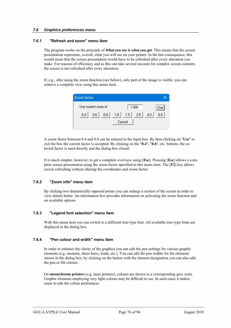
7.6 Graphics preferences menu

7.6.1 "Refresh and zoom" menu item

The program works on the principle of What you see is what you get. This means that the screen presentation represents, overall, what you will see on your printer. In the last consequence, this would mean that the screen presentation would have to be refreshed after every alteration you make. For reasons of efficiency and as this can take several seconds for complex screen contents, the screen is not refreshed after every alteration.

If, e.g., after using the zoom function (see below), only part of the image is visible, you can achieve a complete view using this menu item.

A zoom factor between 0.4 and 8.0 can be entered in the input box. By then clicking on "Use" to exit the box the current factor is accepted. By clicking on the "0.4", "0.6", etc. buttons, the se-lected factor is used directly and the dialog box closed.

It is much simpler, however, to get a complete overview using [Esc]. Pressing [Esc] allows a com-plete screen presentation using the zoom factor specified in this menu item. The [F2] key allows screen refreshing without altering the coordinates and zoom factor.

7.6.2 "Zoom info" menu item

By clicking two diametrically opposed points you can enlarge a section of the screen in order to view details better. An information box provides information on activating the zoom function and on available options.

7.6.3 "Legend font selection" menu item

With this menu item you can switch to a different true-type font. All available true-type fonts are displayed in the dialog box.

7.6.4 "Pen colour and width" menu item

In order to enhance the clarity of the graphics you can edit the pen settings for various graphic elements (e.g. moment, shear force, loads, etc.). You can edit the pen widths for the elements shown in the dialog box; by clicking on the button with the element designation you can also edit the pen or fill colours.

On monochrome printers (e.g. laser printers), colours are shown in a corresponding grey scale. Graphic elements employing very light colours may be difficult to see. In such cases it makes sense to edit the colour preferences.


7.6.5 "Mini-CAD toolbar" and "Header toolbar" menu items

Using these two menu items you can add free text to the graphics and add lines, circles, polygons and images (e.g. files in formats BMP, JPG, PSP, etc.). PDF files can also be imported as images. The same pop-up menu opens for both menu items, the icons and functions used are described in more detail in the Mini-CAD manual saved in the 'C:\Program Files (x86)\GGU-Software\ Manuals' folder during installation. The differences between the Mini-CAD and Header CAD are as follows:

Objects created with "Mini-CAD" are based on the coordinate system (generally in me-tres), in which the drawing is produced, and are shown accordingly. You should use the "Mini-CAD toolbar" when you wish to add information to the system (for example, label-ling of slope inclinations or the location of any foundations).

Objects created with the "Header CAD" are based on the page format (in mm). This makes you independent of the coordinate system and keeps you in the same position on the page. You should select the "Header toolbar" if you wish to place general information on the drawing (company logo, report numbers, plan numbers, stamp etc.). Once you have saved the header information to disk (see "Mini-CAD" user manual), you can load it into com-pletely different systems (with different system coordinates). The saved header information will appear in exactly the same position on the page, which greatly simplifies the creation of general page information.

7.6.6 "Toolbar preferences" menu item

After starting the program a horizontal toolbar for menu items appears below the program menu bar. If you would rather work with a popup window with several columns, you can specify your preferences using this menu item. The smart icons can also be switched off.

At the bottom of the program window you find a status bar with further information. You can also activate or switch off the status bar here. The preferences will be saved in the "GGU-LATPILE.alg" file (see menu item "Graphics preferences/Save graphics preferences") and will be active at the next time the program is started.

By clicking on the tools (smart icons) for the menu items you can directly reach most of the pro-gram functions. The meaning of the smart icons appears as a text box if you hover with the mouse pointer over the tools. Some of the tool functions can be activated from the normal menu items.

"Next page"/"Previous page" Using this icon, you can navigate between the individual pages in the tabular representation.

"Select page" If you are in the tabular representation, you can use this icon to jump to a specific page or to return to the normal representation, that is, to the graphics.

"Zoom out" If you have previously zoomed in, this tool returns to a full screen display.

"Zoom (-)"/"Zoom (+)" With the zoom functions you can zoom in or out of parts of the image, by clicking the left mouse button.


"Colour on/off" If you need to remove the colour from the system presentation, to create a black and white print-out, for example, use this on/off switch.

"Move object" Use this icon to position legends and diagrams at the desired position on the output sheet.

"Copy/print area" Use this tool to copy only parts of the graphics in order to paste them, e.g. to a report. You will see information on this function and can then mark an area, which is copied to the clipboard or can be saved in a file. Alternatively you can send the marked area directly to your printer (see "Tips and tricks", Section 8.4).

"Undo" By clicking this icon the last performed change (e.g. movement of graphical elements made using the [F11] function key or the menu item "Graphics preferences/Move objects") can be undone.

"Restore " By clicking this symbol, the last change undo carried out using "Undo" can be restored.


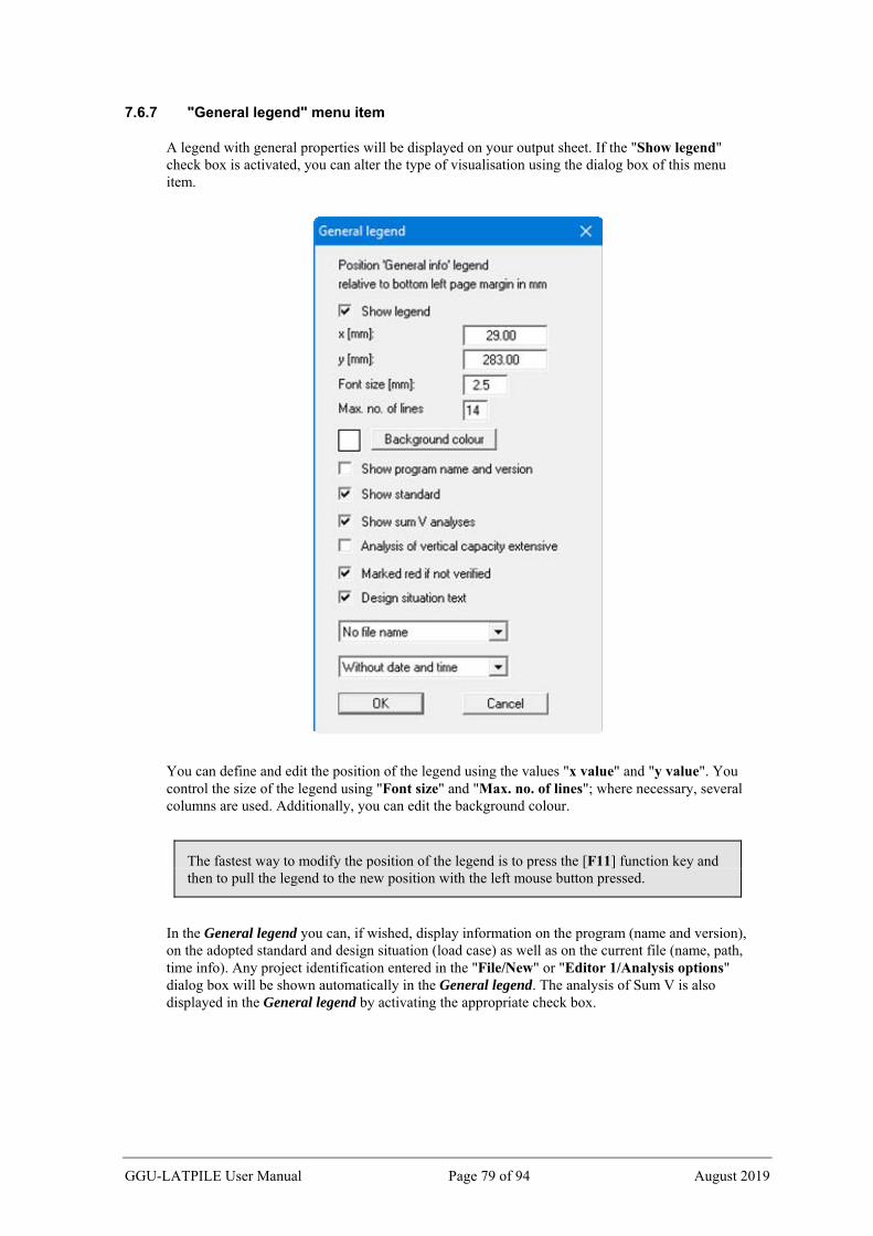
7.6.7 "General legend" menu item

A legend with general properties will be displayed on your output sheet. If the "Show legend" check box is activated, you can alter the type of visualisation using the dialog box of this menu item.

You can define and edit the position of the legend using the values "x value" and "y value". You control the size of the legend using "Font size" and "Max. no. of lines"; where necessary, several columns are used. Additionally, you can edit the background colour.

The fastest way to modify the position of the legend is to press the [F11] function key and then to pull the legend to the new position with the left mouse button pressed.

In the General legend you can, if wished, display information on the program (name and version), on the adopted standard and design situation (load case) as well as on the current file (name, path, time info). Any project identification entered in the "File/New" or "Editor 1/Analysis options" dialog box will be shown automatically in the General legend. The analysis of Sum V is also displayed in the General legend by activating the appropriate check box.


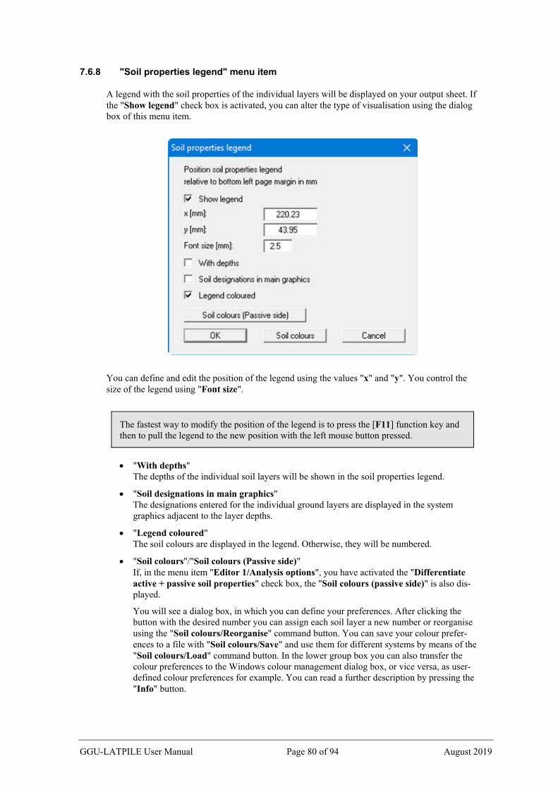
7.6.8 "Soil properties legend" menu item

A legend with the soil properties of the individual layers will be displayed on your output sheet. If the "Show legend" check box is activated, you can alter the type of visualisation using the dialog box of this menu item.

You can define and edit the position of the legend using the values "x" and "y". You control the size of the legend using "Font size".

The fastest way to modify the position of the legend is to press the [F11] function key and then to pull the legend to the new position with the left mouse button pressed.

"With depths" The depths of the individual soil layers will be shown in the soil properties legend.

"Soil designations in main graphics" The designations entered for the individual ground layers are displayed in the system graphics adjacent to the layer depths.

"Legend coloured" The soil colours are displayed in the legend. Otherwise, they will be numbered.

"Soil colours"/"Soil colours (Passive side)" If, in the menu item "Editor 1/Analysis options", you have activated the "Differentiate active + passive soil properties" check box, the "Soil colours (passive side)" is also dis-played.

You will see a dialog box, in which you can define your preferences. After clicking the button with the desired number you can assign each soil layer a new number or reorganise using the "Soil colours/Reorganise" command button. You can save your colour prefer-ences to a file with "Soil colours/Save" and use them for different systems by means of the "Soil colours/Load" command button. In the lower group box you can also transfer the colour preferences to the Windows colour management dialog box, or vice versa, as user-defined colour preferences for example. You can read a further description by pressing the "Info" button.


7.6.9 "Design legend" menu item

Following analysis and design a legend containing the principal system design results is displayed on the screen. Using this menu item you can alter the type of presentation if the "Show legend" check box is activated.

You can define and edit the position of the legend using the values "x value" and "y value". You control the size of the legend using "Font size" and "Max. no. of lines"; where necessary, several columns are used. The fastest way to modify the position of the legend is to press the [F11] func-tion key and then to pull the legend to the new position with the left mouse button pressed.

7.6.10 "Subgrade modulus legend" menu item

A legend is displayed on the screen containing the subgrade reaction moduli entered for the sec-tions along the pile defined for the subgrade reaction profile. Using this menu item you can alter the type of presentation if the "Show legend" check box is activated.

You can define and edit the position of the legend using the values "x" and "y". The size of the legend is controlled by the values for "Font size". The fastest way to modify the position of the legend is to press the [F11] function key and then to pull the legend to the new position while holding the left mouse button.

7.6.11 "Section legend" menu item

A legend containing a small sketch of the pile section employed is displayed on the screen. Using this menu item you can alter the type of presentation or turn off the legend completely.

You can define and edit the position of the legend using the values "x" and "y". The size of the legend is controlled by the height-width ratio. The fastest way to modify the position of the legend is to press the [F11] function key and then to pull the legend to the new position while holding the left mouse button.


7.6.12 "Move objects" menu item

Select this menu item in order to position legends, diagrams and other graphical elements at the desired position on the output sheet. You can also move objects by pressing [F11] and then posi-tioning the legend box with the left mouse button pressed. In that case an info-box appears no more.

If "Manual graph positioning" has been selected in the "System/Graph positioning prefer-ences" menu item (see Section 7.4.7), the result graphs can also be repositioned using this func-tion.

7.6.13 "Save graphics preferences" menu item

Some of the preferences you made with the menu items of the "Graphics preferences" menu can be saved to a file. If you select "GGU-LATPILE.alg" as file name, and save the file on the same level as the program, the data will be automatically loaded the next time the program is started and need not be entered again.

If you do not go to "File/New" upon starting the program, but open a previously saved file instead, the preferences used at the time of saving are shown. If subsequent changes in the general preferences are to be used for existing files, these preferences must be imported us-ing the menu item "Graphics preferences/Load graphics preferences".

7.6.14 "Load graphics preferences" menu item

You can reload a graphics preferences file into the program, which was saved using the "Graph-ics preferences/Save graphics preferences" menu item. Only the corresponding data will be refreshed.


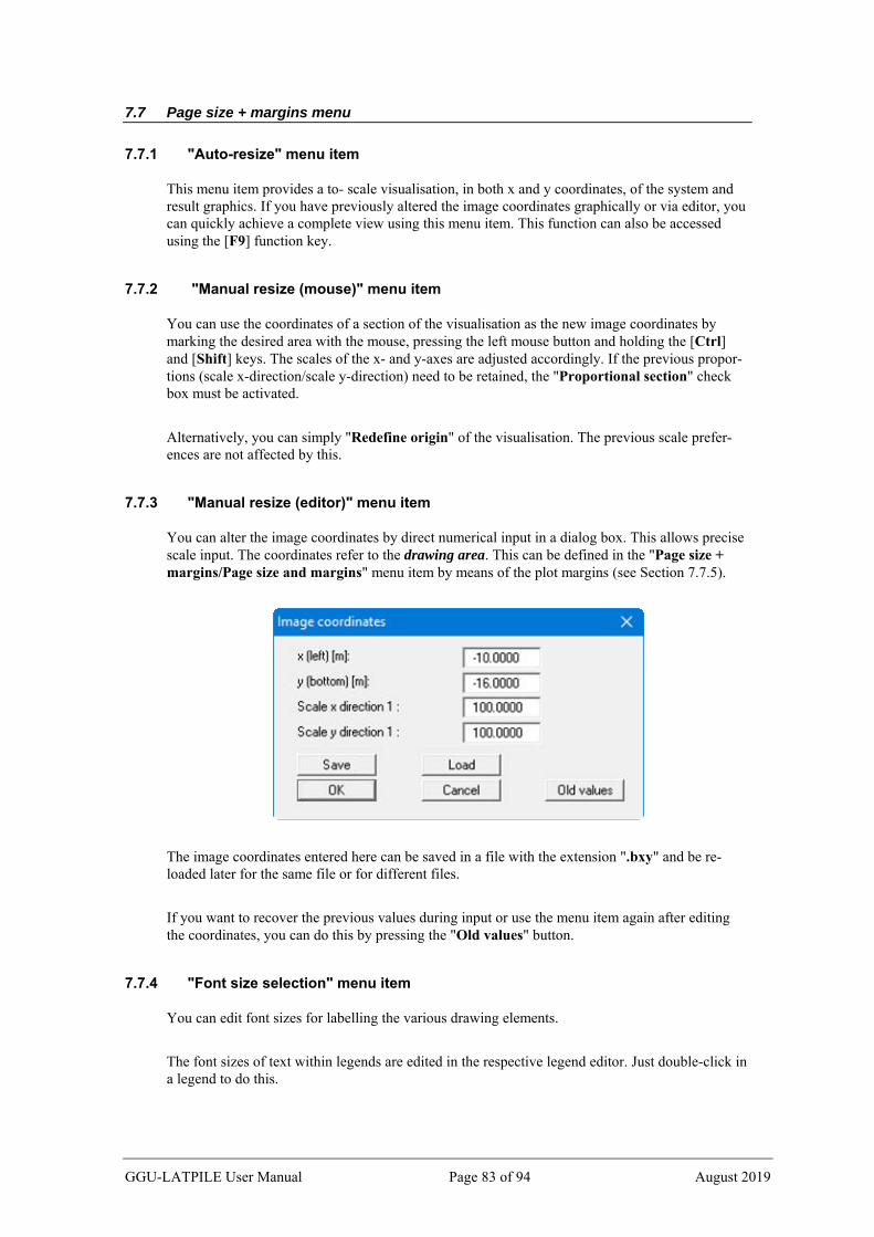
7.7 Page size + margins menu

7.7.1 "Auto-resize" menu item

This menu item provides a to- scale visualisation, in both x and y coordinates, of the system and result graphics. If you have previously altered the image coordinates graphically or via editor, you can quickly achieve a complete view using this menu item. This function can also be accessed using the [F9] function key.

7.7.2 "Manual resize (mouse)" menu item

You can use the coordinates of a section of the visualisation as the new image coordinates by marking the desired area with the mouse, pressing the left mouse button and holding the [Ctrl] and [Shift] keys. The scales of the x- and y-axes are adjusted accordingly. If the previous propor-tions (scale x-direction/scale y-direction) need to be retained, the "Proportional section" check box must be activated.

Alternatively, you can simply "Redefine origin" of the visualisation. The previous scale prefer-ences are not affected by this.

7.7.3 "Manual resize (editor)" menu item

You can alter the image coordinates by direct numerical input in a dialog box. This allows precise scale input. The coordinates refer to the drawing area. This can be defined in the "Page size + margins/Page size and margins" menu item by means of the plot margins (see Section 7.7.5).

The image coordinates entered here can be saved in a file with the extension ".bxy" and be re-loaded later for the same file or for different files.

If you want to recover the previous values during input or use the menu item again after editing the coordinates, you can do this by pressing the "Old values" button.

7.7.4 "Font size selection" menu item

You can edit font sizes for labelling the various drawing elements.

The font sizes of text within legends are edited in the respective legend editor. Just double-click in a legend to do this.


7.7.5 "Page size and margins" menu item

The default page set-up is A3 when the program is started. You can edit the page format in the following dialog box.

"Page in general" defines the size of the output sheet. The A3 format is set as default. The program automatically draws thin cutting borders around the page, which are required when using a plotter on paper rolls. The borders can be switched off using the "With bor-ders" check box.

"Page margin" defines the position of a frame as a distance to the margins. This frame en-closes the subsequent diagram. You can switch off the frame deactivating the "With mar-gins" check box.

The "Plot margin" define a set distance between the page margin and the actual drawing area in which the graphical evaluation of your input is presented.


7.7.6 "Undo" menu item

If you have carried out any changes to dialog boxes or moved objects to a different position on the screen after selecting the "Graphics preferences/Move objects" menu item or using the [F11] function key, this menu item will allow you to undo the movements. This function can also be reached by using the key combination [Alt] + [Back] or the appropriate tool in the toolbar (see Section 7.6.6).

7.7.7 "Restore" menu item

When this menu item is selected the last change made in a dialog box or the last change in the position of objects, which you undid using the menu item "Page size + margins/Undo" will be restored. This function can also be reached by using the key combination [Ctrl] + [Back] or the appropriate tool in the toolbar (see Section 7.6.6).

7.7.8 "Preferences" menu item

You can activate or deactivate the undo functions.

7.8 Info menu

7.8.1 "Copyright" menu item

You will see a copyright message and information on the program version number.

The "System" button shows information on your computer configuration and the folders used by GGU-LATPILE.

7.8.2 "GGU on the web" menu item

Using this menu item you can access the GGU Software website: www.ggu-software.com.

Get information on updates and modifications on a regular basis from your program module page. You can also subscribe to email notifications, which provide information on all modifications on a monthly basis.

7.8.3 "GGU support" menu item

This menu item takes to the GGU-Software Contact area at www.ggu-software.com.

7.8.4 "Maxima" menu item

Here you can check the defaults for maximum values.


7.8.5 "Compare earth pressure coefficients" menu item

Here you can calculate the earth pressure coefficients for given values of phi, delta and beta.

7.8.6 "kh method" menu item

Using this menu item, you can design according to the kh method (DIN 1045 old), independent of any calculated internal forces.

7.8.7 "M-N diagram" menu item

Using this menu item, you can design circular cross- sections according to DIN 1045 (old), inde-pendent of any calculated internal forces. The program calculates steel and concrete strains by means of iteration and from this determines the necessary reinforcement for a symmetrically rein-forced circular cross section. Using this routine, you no longer need to rely on barely readable literature diagrams, but can now also design reinforcement that is not given as diagrams the con-ventional literature.

7.8.8 "Steel design to EC3" menu item

You can perform steel design to EC3 for a different section. You will see the same dialog box as in the menu item "System/Design defaults" (see Section 7.4.6).

7.8.9 "Help" menu item

The GGU-LATPILE manual is opened as a PDF document. The help function can also be ac-cessed using the [F1] function key.

7.8.10 "What's new?" menu item

You will see information on program improvements in comparison to older versions.

7.8.11 "Language preferences" menu item

This menu item allows you to switch the menus and the graphics from German to English and vice versa. To work in German, deactivate the two check boxes Dialoge + Menüs übersetzen (trans-late dialogs, menus)" und "Graphiktexte übersetzen (translate graphics)".

Alternatively, you can work bilingually, e.g. with German dialog boxes but with graphic output in English. The program always starts with the language setting applicable when it was last ended.


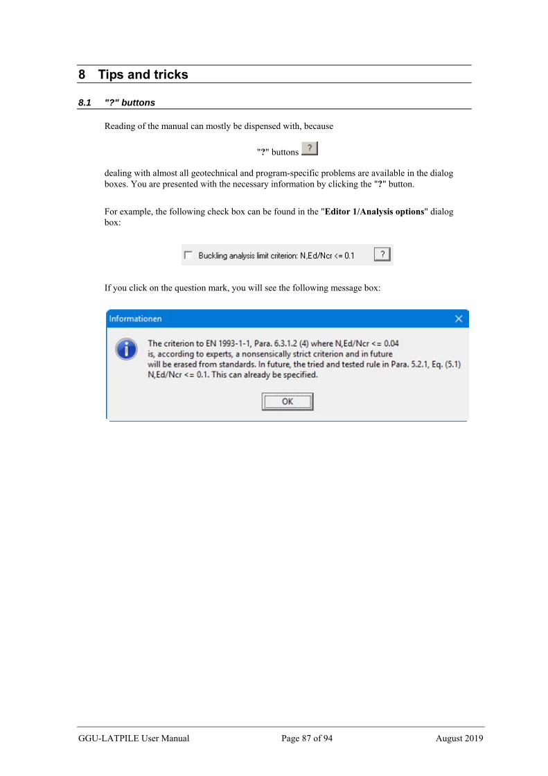
8 Tips and tricks

8.1 "?" buttons

Reading of the manual can mostly be dispensed with, because

"?" buttons

dealing with almost all geotechnical and program-specific problems are available in the dialog boxes. You are presented with the necessary information by clicking the "?" button.

For example, the following check box can be found in the "Editor 1/Analysis options" dialog box:

If you click on the question mark, you will see the following message box:


8.2 Keyboard and mouse

If you click the right mouse button anywhere on the screen a context menu containing the princi-pal menu items opens.

By double-clicking the left mouse button on legends or Mini-CAD objects, the editor for the se-lected element immediately opens, allowing it to be edited.

If you double-click in the system graphics with the left mouse button you will see a message box with the results at the selected depth. This gives you a quick overview of the results for any de-sired depth.

You can scroll the screen with the keyboard using the cursor keys and the [Page up] and [Page down] keys. By clicking and pulling with the mouse, with [Ctrl] pressed, you activate the zoom function, i.e. the selected section will fill the screen. Use the mouse wheel to zoom in or out of the screen view or to pan.


In addition, scale and coordinates of the system graphics (drawing area within the plotting mar-gins) can be altered directly using the mouse wheel. The following mouse wheel functions are available:

Change system graphics (new values can be checked in "Page size + margins/Manual resize (editor)"):

[Ctrl] + mouse wheel up = enlarge system graphics (change of scale)

[Ctrl] + mouse wheel down = shrink system graphics (change of scale)

[Shift] + mouse wheel up = move system graphics up (change in system coordinates)

[Shift] + mouse wheel down = move system graphics down (change in system coordinates)

[Shift] + [Ctrl] + mouse wheel up = move system graphics right (change in system coordinates)

[Shift] + [Ctrl] + mouse wheel down = move system graphics left (change in system coordinates)

Change screen coordinates:

Mouse wheel up = move screen image up

Mouse wheel down = move screen image down

[Alt] + [Ctrl] + mouse wheel up = enlarge screen image (zoom in)

[Alt] + [Ctrl] + mouse wheel down = shrink screen image (zoom out)

[Alt] + [Shift] + mouse wheel up = move screen image right

[Alt] + [Shift] + mouse wheel down = move screen image left

8.3 Function keys

Some of the function keys are assigned program functions. The allocations are noted after the corresponding menu items. The individual function key allocations are:

[Esc] refreshes the screen contents and sets the screen back to your current zoom, which has the default value 1.0. This is useful if, for example, you have used the zoom function to display parts of the screen and would like to quickly return to a complete overview.

[F1] opens the manual file.

[F2] refreshes the screen without altering the current magnification.

[F5] opens the menu item "System/Analyse".

[F6] opens the menu item "Evaluation/Main output summary".

[F7] opens the menu item "System/Optimise".

[F9] opens the menu item "Page size + margins/Auto-resize".

[F11] activates the menu item "Graphics preferences/Move objects".


8.4 "Copy/print area" icon

A dialog box opens when the "Copy/print area" icon in the menu toolbar is clicked, de-scribing the options available for this function. For example, using this icon it is possible to either copy areas of the screen graphics and paste them into the report, or send them directly to a printer.

In the dialog box, first select where the copied area should be transferred to: "Clipboard", "File" or "Printer". The cursor is displayed as a cross after leaving the dialog box and, keeping the left mouse button pressed, the required area may be enclosed. If the marked area does not suit your requirements, abort the subsequent boxes and restart the function by clicking the icon again.

If "Clipboard" was selected, move to the MS Word document (for example) after marking the area and paste the copied graphics using "Edit/Paste".

If "File" was selected, the following dialog box opens once the area has been defined:

The default location of the file is the folder from which the program is started and, if several files are created, the file is given the file name "Image0.emf" with sequential numbering. If the "Rename" button in the dialog box is clicked, a file selector box opens and the copied area can be saved under a different name in a user-defined folder. Saving can be aborted by pressing the "De-lete" button.

If the "Printer" button was pressed in the first dialog box, a dialog box for defining the printer settings opens after marking the area. Following this, a dialog box for defining the image output settings opens. After confirming the settings the defined area is output to the selected printer.


9 Index

2 2nd order theory,

for pile analysis under buckling loads.......... 33 select for analysis ................................... 47, 66

A Absolute heights, use........................................ 38 Action boundary conditions,

defaults at pile toe ........................................ 25 define along pile........................................... 58 define at pile head ........................................ 47

Active earth pressure, analysis principles ........................................ 26 edit preferences ............................................ 51 select for analysis ......................................... 50

Analysis of Sum V, activate/edit preferences................... 55, 56, 74 show results in a message box...................... 75 show results in legend .................................. 79

Analysis of vertical capacity, enter soil properties ................................ 26, 49

Analysis, save results in file ............................. 39 Area loads,

consider as live loads ................................... 59 consider in analysis ...................................... 29 define ........................................................... 59

At rest earth pressure, coefficient after Franke ................................ 26 vert./horiz. component ................................. 26

At-rest earth pressure, select for analysis ......................................... 50

B Bending line,

calculation with Young's modulus ............... 63 Berms,

define labelling preferences ......................... 72 define on active side..................................... 48 define on passive side................................... 48

Bounded surcharges, consider .................................................. 31, 32 define ........................................................... 60

Buckling analysis to DIN EN 1993-1-1, activate ......................................................... 66 pile analysis principles ................................. 33

Buckling analysis, select method for analysis ............................ 63

C Caquot/Kerisel,

passive earth pressure analysis..................... 27 select for analysis ......................................... 52

Clipboard .......................................................... 44 Cohesion coefficient, determination methods... 26 Cohesion,

enter/adopt from soil database...................... 49

Colour, define for soils.............................................. 80 switch on/off .......................................... 78, 80

Colour/hatching, define for loads ..................... 71 Colour/pens, define for graphical elements ...... 76 Company letterhead, add via Mini-CAD.......... 77 Cone resistance,

for analysis of vertical capacity.............. 26, 49 Context menu, open.......................................... 88 Coordinates,

alter via editor .............................................. 83 alter with mouse ........................................... 83 optimise/reset ............................................... 83 save/load ...................................................... 83

Copy/print area ..................................... 44, 78, 90 Culmann,

earth pressure calculation ............................. 27 Cutting borders, switch on/off .......................... 84

D Damping, define for iteration ........................... 19 Database,

for soil properties of common soils .............. 49 Dataset description,

display .......................................................... 79 enter.............................................................. 37

Delete, soil layers ..................................................... 50 steel sections ................................................ 61

Design passive earth pressure, in analysis ........ 66 Design section, select ................................. 61, 62 Design situation,

activate display in legend ............................. 79 enter text for legend ..................................... 56

Design, display results in legend ............................... 81 of circular cross-sections.............................. 86 using kh method ........................................... 86

Differential equation, elastically embedded pile ............................. 25

Dimension lines, define............................................................ 73 move with mouse ......................................... 82

DIN 4085, consider in analysis ................................ 26, 27 select for analysis ......................................... 52

DIN EN 1993-5/DIN EN 1993-1-1................... 33 Displacement boundary conditions, define....... 58 Displacement, define for pile............................ 58 Distributed load,

define............................................................ 48 define labelling preferences ......................... 72

Drawing area, define......................................... 84 DXF file,

export ........................................................... 44 import ............................................................. 7

Dynamic wind loading, consider using a factor ................................. 47


E Earth pressure coefficients,

be analysed................................................... 86 calculate ....................................................... 53 user-defined.................................................. 53

Earth pressure, after Culmann............................................... 27 preferences for active ................................... 51 preferences for passive ................................. 52 select for analysis ......................................... 50

Earth quake, as design situation to EC 7 ........................... 56 consider loads............................................... 54

EC 2, cross-section approach............................ 38 EC 3, activate for steel design .......................... 38 EC 7, load cases description ............................. 56 Design,.............................................................. 68 Editor window, output table ............................. 42 Elastically embedded pile,

differential equation ..................................... 25 EMF format ...................................................... 44 Equivalent earth pressure coefficient,

activate use................................................... 51 Euler cases, example files................................. 36 Excavation, change alignment .......................... 38

F FGSV.................................................................. 6 File,

display name in legend................................. 79 load/save ...................................................... 39

Find optimum section ................................. 19, 68 Finite element method ...................................... 25 First moment of area, enter for steel sections ... 62 Font selection ................................................... 76 Font size,

design legend................................................ 81 dimension lines ............................................ 73 edit for graphical elements ........................... 83 general legend .............................................. 79 soil properties legend ................................... 80 subgrade modulus legend ............................. 81 system/result graphics .................................. 72

Footer, output table........................................... 40 Franke............................................................... 26 Friction angle,

activate separate act./pass. values input ....... 38 enter/adopt from soil database...................... 49

Function keys ................................................... 89

G General page information,

add via Mini-CAD........................................ 77 General stability, verification via file export .... 43 GGU-CAD file, export ..................................... 44 GGUMiniCAD file, export............................... 45 GGU-STABILITY file, export ......................... 43 Global coordinates,

use for Mini-CAD output ............................. 45 Global safety factors concept,

select for analysis ......................................... 37

Graph grids, define ........................................... 72 Graph positions,

alter via editor .............................................. 70 alter with mouse ........................................... 82

Graphics, add via Mini-CAD............................ 77 Groundwater,

define............................................................ 48 define colour ................................................ 76 define labelling preferences ......................... 72

H Hatching, define for loads ................................ 71 Header CAD, application explanations ............ 77 Header, output table.......................................... 40 Horizontal displacement, define for pile head .. 25 Horizontal force, define at pile head................. 47

I Increased active earth pressure,

coefficient .................................................... 27 select for analysis ......................................... 50

Iteration, define canceling criteria ............................... 19 define damping............................................. 19 pile optimisation........................................... 68 reduction subgrade reaction moduli ......... 6, 19

K kh method ......................................................... 86

L Labelling, system/result graphics ..................... 72 Language preferences ................................... 7, 86 Lateral pressures, define ................................... 59 Layout,

define for output sheet.................................. 84 define for output table .................................. 40

Legends, move with mouse .............................. 82 Licence protection .............................................. 7 Line loads,

define............................................................ 59 perpendicular to pile axis ............................. 30

Live load, consider area load as .................................... 59 consider distributed load as .......................... 48

Load case, activate display in legend ............................. 79 enter text for legend ..................................... 56

Load case,adopt from DIN 1054-2010/EC 7 .... 56 Load concentration factor,

consider ........................................................ 30 define............................................................ 53

Loads, graphical output preferences ................. 71

M M EBGS-Lsw 2018,

determination of moment/horizontal force ... 47 FGSV Code of Practice .................................. 6

Manual, open as PDF file ................................. 86


Maximum values, display for state variables............................. 74 show for system ........................................... 85

Metafile, export ................................................ 44 Mini-CAD,

application explanations............................... 77 export file ..................................................... 45 output with global coordinates ..................... 45

M-N-diagram.................................................... 86 Moment of inertia,

enter for steel sections.................................. 62 Moment restraint, define................................... 25 Moment, define at pile head ............................. 47 Mouse,

click functions .............................................. 88 wheel functions ............................................ 89

mu ks, enter ...................................................... 57

N Navigation, output table ................................... 77

O Objects, move with mouse................................ 82 ÖNORM EN 1997-1,

select partial safety factors ........................... 56 Output preferences...................................... 42, 43 Output table,

edit output as ASCII..................................... 42 edit output as graphics.................................. 40 navigation..................................................... 41 select output format...................................... 39 switch to system graphics....................... 41, 77

P Page,

copy/print section................................... 78, 90 define format ................................................ 84 switch margins on/off................................... 84

Pagination, automatic ................................. 41, 42 Partial safety factors,

define ........................................................... 56 select from ÖNORM EN 1997-1.................. 56

Passive earth pressure, analysis methods for coefficients ................. 27 spatial effect ................................................. 52 specify calculation........................................ 52

PDF file, import via Mini-CAD.................... 7, 77 Pen preferences, edit for graphical elements .... 76 Pile head,

max. rotation for iteration ............................ 68 Pile head,

define horizontal displacement.................... 25 define moment restraint................................ 25

Pile head, max. displacement for iteration.................... 68

Pile toe, define action boundary conditions...... 25 Pile,

define different sections ............................... 63 define inclination.......................................... 38 define rotation/displacement ........................ 58 define width/length ...................................... 47

optimise length ............................................. 67 select type..................................................... 38

Piling Handbook, consideration of line loads............................ 30 effect on earth pressure ................................ 28

Plausibility checks, view results ....................... 64 Plot margins, define.......................................... 84 Pre-curvature,

activate visualisation in result graphics........ 71 define for buckling analysis ......................... 66 visualisation in different systems ................. 34

Presentation height, loads ................................. 71 Print,

graphics ........................................................ 43 output table................................................... 44 section .............................................. 44, 78, 90 several files .................................................. 46

Program, display name in legend................................. 79 save/load preferences ................................... 82 show improvements...................................... 86 show information ......................................... 85

Project data, add via Mini-CAD ....................... 77 Project identification,

display .......................................................... 79 enter.............................................................. 37

R Reinforced concrete cross-section,

design values ................................................ 65 Result graphics,

alter positions ............................................... 70 display .......................................................... 73 edit preferences ............................................ 71 label.............................................................. 72

Results, display for selected depth.............. 74, 88 Rods, define for system .................................... 64 Rotation, define for pile.................................... 58

S Safety concept, select ....................................... 37 Scale,

alter with mouse ........................................... 83 define via editor ........................................... 83 determine automatically ............................... 83

Scroll the screen ............................................... 88 Section modulus,

enter for steel sections.................................. 62 Section,

activate selection from list............................ 38 display as sketch in legend........................... 81 edit/enlarge list ............................................. 61

Sections, activate design with differing sections ......... 38 optimise length graphically .......................... 75

Seismic acceleration, as design situation to EC 7 ........................... 56 consider loads............................................... 54

Self-weight pile, calculation ............................. 63 Shear strength,

for analysis of vertical capacity.............. 26, 49 Shear stress, values for steel sections ............... 62



Slope stability application ................................ 43 Smarticons, for menu items .............................. 77 Soil colours/numbers, activate display ............. 80 Soil designations,

activate presentation in system graphics ...... 80 enter ............................................................. 49

Soil layers, adapt to absolute heights .............................. 48 define/delete ................................................. 50 maximum number ........................................ 26

Soil properties, define ........................................................... 49 display in legend .......................................... 80 enter/adopt from soil database...................... 49

Soil stress, in analysis....................................... 66 Specific weight, define for sections.................. 63 Standard, display in legend............................... 79 Status bar main program, activate .................... 77 Steel cross-section, select for Sum V................ 74 Steel design, activate to EC 3 ........................... 38 Steel grade, select for analysis.......................... 63 Steel pile,

define different sections ............................... 63 Steel pile, define partial corrosion .................... 63 Steel sections,

define/delete ................................................. 61 select for design ..................................... 61, 62

Streck, passive earth pressure analysis..................... 27 select for analysis ......................................... 52

Subgrade reaction modulus, define profile ................................................ 57 display profile in legend............................... 81 select unit ............................................... 38, 57

Subgrade, reduce ........................................ 18, 66 Sum V,

activate analysis/edit preferences ..... 55, 56, 75 System,

activate coloured display.............................. 80 analyse ................................................... 18, 65 display .......................................................... 73 display properties in legend ......................... 79 division into rods.......................................... 64 edit graphics output preferences................... 71

show information ................................... 64, 85

T Theory of elastic half-space.............................. 30 Toolbar, edit for menu items ............................ 77 Translation, activate ......................................... 86 True-type font................................................... 76 Types of resulting earth pressure distribution... 29

U Unit weight,

activate separate act./pass. values input ....... 38 enter/adopt from soil database...................... 49

V Version number,

display in a message box.............................. 85 display in legend .......................................... 79

Vertical capacity, enter soil properties for analysis............. 26, 49

Vertical force, define at pile head..................... 47

W Web thickness, enter for steel sections ............. 62 Weißenbach, spatial passive earth pressure ...... 27 What you see is what you get ........................... 76 Working capacity,

determine for dolphin analysis ..................... 75

Y Young's modulus,

enter for steel sections.................................. 63

Z Zoom factor, define for full-screen display ...... 76 Zoom function, activate........................ 76, 77, 88

analysis and design of laterally loaded piles ggu-latpile · 2019-09-02 · 1 preface . ggu-latpile...

Documents