analysis and synthesis of 3d shape families via deep

Eurographics Symposium on Geometry Processing 2015Mirela Ben-Chen and Ligang Liu(Guest Editors)

Volume 34 (2015), Number 5

Analysis and synthesis of 3D shape familiesvia deep-learned generative models of surfaces

Haibin Huang Evangelos Kalogerakis Benjamin Marlin

University of Massachusetts Amherst

Figure 1: Given a collection of 3D shapes, we train a probabilistic model that performs joint shape analysis and synthesis.(Left) Semantic parts and corresponding points on shapes inferred by our model. (Right) New shapes synthesized by our model.

AbstractWe present a method for joint analysis and synthesis of geometrically diverse 3D shape families. Our methodfirst learns part-based templates such that an optimal set of fuzzy point and part correspondences is computedbetween the shapes of an input collection based on a probabilistic deformation model. In contrast to previoustemplate-based approaches, the geometry and deformation parameters of our part-based templates are learnedfrom scratch. Based on the estimated shape correspondence, our method also learns a probabilistic generativemodel that hierarchically captures statistical relationships of corresponding surface point positions and parts aswell as their existence in the input shapes. A deep learning procedure is used to capture these hierarchical rela-tionships. The resulting generative model is used to produce control point arrangements that drive shape synthesisby combining and deforming parts from the input collection. The generative model also yields compact shape de-scriptors that are used to perform fine-grained classification. Finally, it can be also coupled with the probabilisticdeformation model to further improve shape correspondence. We provide qualitative and quantitative evaluationsof our method for shape correspondence, segmentation, fine-grained classification and synthesis. Our experimentsdemonstrate superior correspondence and segmentation results than previous state-of-the-art approaches.

Categories and Subject Descriptors (according to ACM CCS): I.3.5 [Computer Graphics]: Computational Geometryand Object Modeling—

1. IntroductionDiscovering geometric and semantic relationships of 3Dshapes is fundamental to several computer graphics appli-cations. In particular, several tools for geometric modeling,manufacturing, shape retrieval and exploration can benefitfrom algorithms that automatically extract part, region andpoint correspondences within large shape collections. Dur-ing the recent years, due to the growing number of online

3D shape repositories (Trimble Warehouse, Turbosquid andso on), a number of algorithms have been proposed to jointlyanalyze shapes in large collections to discover such corre-spondences. The key advantage of these algorithms is thatthey do not treat shapes in complete isolation from eachother, but rather extract useful mappings and correlations be-tween shapes to produce results that are closer to what a hu-man would expect.

c© 2015 The Author(s)Computer Graphics Forum c© 2015 The Eurographics Association and JohnWiley & Sons Ltd. Published by John Wiley & Sons Ltd.

H. Huang & E. Kalogerakis & B. Marlin / Analysis and synthesis of 3D shape familiesvia deep-learned generative models of surfaces

Although there has been significant progress on analy-sis of shapes with similar structure (e.g., human bodies)and similar types of deformations (e.g, isometries or near-isometries), dealing with collections of structurally and geo-metrically diverse shape families (e.g., furniture, vehicles)still remains an open problem. A promising approach tohandle such collections is to iteratively compute part or/andpoint correspondences and existence using part-based or lo-cal non-rigid alignment [KLM∗13, HSG13]. The rationalefor such approach is that part correspondences can help lo-calize point correspondences and improve local alignment,point correspondences can refine segmentations and localalignment, and in turn more accurate local alignment can fur-ther refine segmentations and point correspondences. One ofthe drawbacks of existing methods following this approachis that strict point-to-point correspondences are not that suit-able for collections of shapes whose parts exhibit signifi-cant geometric variability, such as airplanes, bikes and soon. In addition, these methods use templates made out ofbasic primitives (e.g., boxes in [KLM∗13]) or other mediat-ing shapes [HSG13], whose geometry may drastically differfrom the surface geometry of several shapes in the collec-tion leading to inaccurate correspondences. In the case oftemplate fitting, approximate statistics on the used primitivescan be used to penalize unlikely alignments (e.g., Gaussiandistributions on box positions and scales). However, thesestatistics capture rather limited information about the ac-tual surface variability in the shapes of the input collection.Similarly, in the context of shape synthesis, shape variabil-ity is often modeled with statistics over predefined part de-scriptors that cannot be directly mapped back to surfaces[KCKK12] or parameters of simple basic primitives, suchas boxes [FAvK∗14, AKZM14].

We present a method that analyzes and synthesizes 3D shapecollections by learning representations of surface variabil-ity from scratch. Our method has two main components:a probabilistic deformation model and a generative surfacemodel. The probabilistic deformation model jointly esti-mates fuzzy point correspondences and part segmentationsof shapes through learned part-based templates. In contrastto previous works that use simple geometric primitives orpre-existing shapes as templates, our method learns the tem-plate geometry and deformations from the input collection.The deformation model provides input to our generative sur-face model that aims to learn geometric and structural re-lationships of parts and corresponding surface point posi-tions. Following the concept of deep learning (or hierarchi-cal learning) [Ben09] widely used in computer vision andnatural language processing, the key idea of our generativemodel is to learn relationships in the surface data hierarchi-cally: our model learns geometric arrangements of pointswithin individual parts through a first layer of latent vari-ables. Then it encodes interactions between the latent vari-ables of the first layer through a second layer of latent vari-ables whose values correspond to relationships of surface ar-rangements across different parts. Subsequent layers medi-ate higher-level relationships related to the overall shape ge-ometry, semantic attributes and structure. The hierarchicalarchitecture of our model is well-aligned with the composi-tional nature of shapes: shapes usually have a well-definedstructure, their structure is defined through parts, parts are

made of patches and point arrangements with certain regu-larities.

Our method can jointly learn the probabilistic deformationmodel and the generative surface model leading to improvedshape correspondence. In addition, the generative model canbe sampled to generate plausible point-sampled surfaces thatautomatically drive shape synthesis. Finally, its uppermostlayer produces a compact shape descriptor, or feature rep-resentation, that can be used to perform fine-grained clas-sification (e.g., airplanes can be categorized to fighter jets,propeller aircraft, unmanned aerial vehicles, and so on).

Contributions. The contribution of our work is two-fold.First, we provide a probabilistic deformation model that es-timates fuzzy point and part correspondences within struc-turally and geometrically diverse shape families. The maindifference with previous work is that our method learns thegeometry and deformation parameters of templates withina fully probabilistic framework to optimally achieve thesetasks instead of relying on fixed primitives or pre-existingshapes. Second, we introduce a deep-learned probabilisticgenerative model of 3D shape surfaces that can be used tofurther optimize shape correspondences, synthesize surfacepoint arrangements, and produce compact shape descriptorsfor fine-grained classification. Both probabilistic models canbe learned together leading to joint shape analysis and syn-thesis. To the best of our knowledge, our method is the firstto apply deep learning for training generative models of 3Dshape surfaces. In contrast to previous work on generativeprobabilistic models that rely on highly structured databases(e.g., manually segmented shapes), our deep-learned modelsynthesizes shapes without or minimal human supervision.While previous generative models usually encode only high-level part and shape descriptors, our model directly encodessurface geometry and shape structure. Instead of mixing-and-matching parts from a database to synthesize shapes asfrequently done in prior work, the sampled surface point ar-rangements of our model can be used to also deform the in-put collection parts to create more novel shape variations.

2. Related Work

Our method is related to prior work on data-driven meth-ods for computing shape correspondences in collections withlarge geometric and structural variability, statistical modelsof shapes, and deep Boltzmann machines. We review themost relevant work in these areas. A complete review ofprevious research in shape correspondences and segmenta-tion is out of the scope of this paper. We refer the readerto recent surveys in shape correspondences [vKZHCO11],segmentation [TPT15], and structure-aware shape process-ing [MWZ∗13].

Data-driven shape correspondences. Analyzing shapesjointly in a collection to extract useful geometric, struc-tural and semantic relationships often yields significantlybetter results than analyzing isolated single shapes or pairsof shapes, especially for classes of shapes that exhibit largegeometric variability. This has been demonstrated in pre-vious data-driven methods for computing point-based andfuzzy correspondences [KLM∗12,HZG∗12,HSG13,HG13].However, these methods do not leverage the part structure

c© 2015 The Author(s)Computer Graphics Forum c© 2015 The Eurographics Association and John Wiley & Sons Ltd.


of the input shapes and do not learn a model of surfacevariability. As a result, these methods often do not gener-alize well to collections of shapes with significant struc-tural diversity. A number of data-driven methods have beendeveloped to segment shapes and effectively parse theirstructure [KHS10, HKG11, SvKK∗11, HFL12, WAvK∗12,LMS13, XSX∗14, XXLX14]. However, these methods buildcorrespondences only at a part level, thus cannot be usedto find more fine-grained point or region correspondenceswithin parts. Some of these methods require several train-ing labeled segmentations [KHS10, vKZHCO11, XXLX14]as input, or require users to interactively specify tens to hun-dreds of constraints [WAvK∗12].

Our work is closer to that of Kim et al. [KLM∗13]. Kim etal. proposed a method that estimates point-level correspon-dences, part segmentations, rigid shape alignments, and astatistical model of shape variability based on template fit-ting. The templates are made out of boxes that iteratively fitto segmented parts. Boxes are rather coarse shape represen-tations and in general, shape parts frequently have drasticallydifferent geometry than boxes. Our method also makes useof templates to estimate correspondences and segmentations,however, their geometry and deformations are learned fromscratch. Our produced templates are neither pre-existingparts nor primitives, but new learned parts equipped withprobabilities over their point-based deformations. Kim etal.’s statistical model learns shape variability only in termsof individual box parameters (scale and position) and can-not be used for shape synthesis. In contrast, our statisticalmodel encodes both shape structure and actual surface ge-ometry, thus it can be used to generate shapes. Kim et al.’smethod computes hard correspondences via closest points,which are less suitable for typical online shape repositoriesof inanimate objects. Our method instead infers probabilis-tic, or fuzzy, correspondences and segmentations via a prob-abilistic deformation model that combines non-rigid surfacealignment, feature-based matching, as well as a deep-learnedstatistical model of surface geometry and shape structure.

Statistical models of 3D shapes. Early works developedstatistical models of shapes in specific domains, such asfaces [BV99], human bodies [ACP03], and poses [ASK∗05].Yingze et al. [BCLS13] proposed a statistical model ofsparse sets of anchor points by deforming a mean tem-plate shape using thin-plate spline (TPS) transformations forshapes, like cars, fruits, and keyboards. Our work can beseen as a generalization of these previous works to domainswhere shapes differ in both their structure and geometry andwhere no single template or mean shape can be used.

A number of approaches have tried to model shape variabil-ity using Principal Component Analysis or Gaussian Pro-cess Latent Variable models on Signed Distance Function(SDF) representations of shapes [SDYT11, CKC11, PR11,DPRR13]. However, the dimensionality of SDF voxel-basedrepresentations is very high, requiring the input shapes tobe discretized at rather coarse voxel grids or use compres-sion schemes that tend to eliminate surface features of theoutput shapes. Various ad-hoc weights are frequently usedto infer coherent SDF values for the output shapes. Othermethods use deformable templates made out of orientedboxes [OLGM11, KLM∗13, AKZM14], and model shape

variability in terms of the size and position of these boxes.Xu et al. [XZCOC12] mixes-and-matches parts through setevolution with part mutations (or deformations) followingthe box parametrization approach of [OLGM11] and partcrossovers controlled by user-speficied fitness scores. Fishet al. [FAvK∗14] and Yumer et al. [YK14] represent shapesin terms of multiple basic primitives (boxes, planes, cylin-ders etc) and capture shape variability in terms of primi-tive sizes, relative orientations, and translations. As a result,these methods do not capture statistical variability at the ac-tual surface level and cannot directly be used to generate newsurface point arrangements. Kalogerakis et al. [KCKK12]proposed a generative model of shape structure and part de-scriptors (e.g., curvature histograms, shape diameter, silhou-ette features). However, these descriptors are not invertiblei.e., they cannot be directly mapped back to surface points.As a result, their model cannot be used to output surfacegeometry and was only used for shape synthesis by retriev-ing and recombining database parts without further modifi-cations. In constrast to the above approaches, our generativemodel jointly analyzes and synthesizes 3D shape families,outputs both structure and actual surface geometry, as wellas learned class-specific shape descriptors.

Deep Boltzmann Machines. The statistical model of sur-face variability proposed in our paper follows the structure ofa general class of probabilistic generative models, known asDeep Boltzmann Machines (DBMs) in the machine learningliterature. DBMs have showed promising results for speechand image generation [RSMH11,RHSW11,MDH12,SH12].In a concurrent work, Wu et al. [WSK∗15] proposed DBMsbuilt over voxel representations of 3D shapes to producegeneric shape descriptors and reconstruct low-resolutionshapes from input depth maps. Our model in inspired byprior work on DBMs to develop a deep generative model of3D shape surfaces. Our model has several differences com-pared to previous DBM formulations. Our model aims atcapturing continuous variability of surfaces, instead of pixelor voxel interactions. To capture surface variability, we useBeta distributions to model the surface point locations (in-stead of Gaussian or Bernoulli distributions frequently usedin DBMs). In addition, the connectivity of layers in ourmodel takes into account the structure of shapes based ontheir parts. Since shape collections have typically a muchsmaller size than image or audio collections, and since thegeometry of surfaces tend to vary smoothly across neighbor-ing points, we use spatial smoothness priors during training.We found that all these adaptations were important to gener-ate surface geometry.

3. Overview

Given a 3D model collection representative of a shape fam-ily, our goal is to compute probabilistic point correspon-dences and part segmentations of the input shapes (Figure1, left), as well as learn a generative model of 3D shapesurfaces (Figure 1, right). At the heart of our method liesa probabilistic deformation model that learns part templatesand uses them to compute fuzzy point correspondences andsegmentations. We now provide an overview of our part tem-plate learning concept, our probabilistic deformation model,and our generative surface model.



(a)

(b)

(c)

legs seat back armrests columm base

Figure 2: Hierarchical part template learning for a collec-tion of chairs. (a) Learned high-level part templates for allchairs. (b) Learned part templates per chair type or group(benches, four-legged chairs, office chairs). (c) Representa-tive shapes per group and exemplar segmented shapes (inred box).

Learned part templates. Our method computes probabilis-tic surface correspondences by learning suitable part tem-plates from the input collection. As part template, we de-note a learned arrangement of surface points that can beoptimally deformed towards corresponding parts of the in-put shapes under a probabilistic deformation model. To ac-count for structural differences in the shapes of the inputcollection, the part templates are learned with a hierarchi-cal procedure. Our method first clusters the input collectioninto groups containing structurally similar shapes, such asbenches, four-legged chairs and office chairs (Figure 2c).Then a template for each semantic part per cluster is learned(Figure 2b). Given the learned group-specific part templates,our method learns higher-level templates for semantic partsthat are common across different groups e.g. seats, backs,legs, armrests in chairs (Figure 2a). The top-level part tem-plates allow our method to establish correspondences be-tween shapes that belong to structurally different groups,yet share parts under the same label. If parts are unique toa group (e.g., office chair bases), we simply transfer them tothe top level and do not establish correspondences to incom-patible parts with different label coming from other clusters.

Probabilistic deformation model. At the heart of our algo-rithm lies a probabilistic deformation model (Section 4). Themodel evaluates the probability of deformations applied onthe part templates under different corresponding point andpart assignments over the input shape surfaces. By perform-ing probabilistic inference on this model, our method itera-tively computes the most likely deformation of the part tem-plates to match the input shape parts (Figure 3). At each it-eration, our method deforms the part templates, and updatesprobabilities of point and part assignments over the inputshape surfaces. The updated probabilistic point and part as-signments iteratively guides the deformation and vice versauntil convergence.

Generative surface model. Based on the estimated proba-bility distributions over corresponding point and part assign-ments on all the input shapes of the collection, our methodlearns a probabilistic model characterizing the structural andsurface variability within a shape family (Section 5). The

surface variability is encoded in the model through a jointprobability distribution that captures relationships betweenparts and surface point locations within the shape family.For example, consider airplanes. The position of wingtipsis strongly related to the positions of other points on thesame wing (i.e., the overall wing geometry), as well as thepart arrangement and surface geometry of the whole air-plane. These complex relationships of points and parts inthe shapes of a family are hierarchically captured throughlatent variables. The model contains a layer of latent vari-ables whose assignments are associated with arrangementsof surface points within the same part. Higher-level layers oflatent variables progressively capture relationships betweensurface points belonging to different shape parts. The la-tent variables also capture dominant modes of surface pointarrangements corresponding to structurally different shapegroups. By sampling the latent variables on the top layer, ourmodel can generate parts and surface points that are used tosynthesize new shapes. The top layer also produces shapedescriptors that can be used for fine-grained classification.Through the captured relationships between point locations,the model can be used to further improve correspondencesin the shapes of the collection.

Pre-processing. Our method requires the following pre-processing, or initialization: first, we rely on the rigid align-ments provided by Kim et al. [KLM∗13] to consistently ori-ent the input shapes of each collection. Practically, we foundthat our surface variability model can tolerate incorrectlyaligned shapes in the collections (e.g. about 5% of the inputshapes were not aligned correctly in the dataset it was trainedon). Second, our method requires as input a labeled segmen-tation for at least one shape per group (Figure 2c, red boxes).The segmentation can be provided by either the user, or anautomatic co-segmentation technique. In the case of manualinput, to facilitate the user, our method automatically clus-ters the shapes into groups and selects an exemplar shape pergroup. The user is asked to segment these exemplar shapes.In the case of co-segmented input, we use the segmentationsprovided by Kim et al. [KLM∗13]. We note that the pro-vided segmentations are used for initialization only: giveninitial segments, our methods learns the part templates andimproves the shape segmentations.

4. Probabilistic deformation model

Our method takes as input a collection of shapes, and outputsgroups of structurally similar shapes together with learnedpart templates per group (Figure 2). Given the group-specificpart templates, our method also outputs high-level part tem-plates for the whole collection. A probabilistic model isused to infer the part templates. The model evaluates thejoint probability of hypothesized part templates, deforma-tions of these templates towards the input shapes, as well asshape correspondences and segmentations. The probabilisticmodel is defined over the following set of random variables:

Part templates Y = {Yk} where Yk ∈ R3 denotes the 3Dposition of a point k on a latent part template. There aretotal K such variables, where K is the number of points onall part templates. The number of points per part templateis determined from the provided exemplar shape parts.



learned parttemplates

input shape

deformed part templates (iteration 1)



prob. pointcorrespondences

prob. segmentation


prob. segmentation


prob. segmentation

Figure 3: Given learned part templates for four-leggedchairs, our method iteratively deforms them towards an in-put shape through probabilistic inference. At each itera-tion, probability distributions over deformations, point cor-respondences and segmentations are inferred according toour probabilistic model (probabilistic correspondences areshown only for the points appearing as blue spheres on thelearned part templates).

Deformations D = {Dt,k} where Dt,k ∈ R3 represents theposition of a point k on a part template as it deforms to-wards the shape t. Given T input shapes and K total pointsacross all part templates, there are K ·T such variables.

Point correspondences U = {Ut,p} where Ut,p ∈{1,2, ...,K} represents the “fuzzy” correspondenceof the surface point p on an input shape t with pointson the part templates. In our implementation, each inputshape is uniformly sampled with 5000 points, thus thereare total 5000 ·T such random variables.

Surface segmentation S = {St,p} where St,p ∈ {1, ...,L}represents the part label for a surface point p on an in-put shape t. L is the number of available part templates,corresponding to the total number of semantic part labels.There are also 5000 ·T surface segmentation variables.

Input surface points Xt = {Xt,p} where Xt,p ∈ R3 repre-sents the 3D position of a surface sample point p on aninput shape t.

Our deformation model is defined through a set of factors,each representing the degree of compatibility of different as-signments to the random variables it involves. The factorscontrol the deformation of the part templates, the smooth-ness of these deformations, the fuzzy point correspondencesbetween each part template and input shape, and the shapesegmentations. The factors are designed out of intuition andexperimentation. We now explain the factors used in ourmodel in detail.

Unary deformation factor. We first define a factor that as-sesses the consistency of deformations of individual surfacepoints on the part templates with an input shape. Given aninput shape t represented by its sampled surface points Xt ,the factor is defined as follows:

φ1(Dt,k,Xt,p,Ut,p = k) =

exp{− .5(Dt,k−Xt,p)

TΣ−11 (Dt,k−Xt,p)

}where the parameter Σ1 is a diagonal covariance matrix es-timated automatically, as we explain below. The factor en-

courages deformations of points on the part templates to-wards the input shape points that are closest to them.

Deformation smoothness factor. This factor encouragessmoothness in the deformations of the part templates. Givena pair of neighboring surface points k,k′ on an input tem-plate, the factor is defined as follows:

φ2(Dt,k,Dt,k′ ,Yk,Yk′) =

exp{− .5((Dt,k−Dt,k′)− (Yk−Yk′))

TΣ−12

((Dt,k−Dt,k′)− (Yk−Yk′))

}The factor favors locations of deformed points relative totheir deformed neighbors that are closer to the ones on the(undeformed) part templates. The covariance matrix Σ2 isdiagonal and is also estimated automatically. In our imple-mentation, we use the 20 nearest neighbors of each point kto define its neighborhood.

Correspondence factor. This factor evaluates the compati-bility of a point on a part template with an input surface pointby comparing their geometric descriptors:

φ3(Ut,p = k,Xt) = exp{− .5(fk− ft,p)

TΣ−13 (fk− ft,p)

}where fk and ft,p are geometric descriptors evaluated onthe points of the part template and the input surface Xtrespectively, Σ3 is a diagonal covariance matrix. Our de-scriptor includes geometric information from shape diam-eter [SSCO08] (under three different normalizing parame-ters α = 1,2,4), average geodesic distance [HSKK01], andPCA [KLM∗13], forming a 10− dimensional vector.

Segmentation factor. This factor assesses the consistency ofeach part label with an individual surface point on an inputshape. The part label depends on the fuzzy correspondencesof the point with each part template:

φ4(St,p = l,Ut,p = k) ={

1, if label(k) = lε, if label(k) 6= l

where label(k) represents the label of the part template withthe point k. The constant ε is used to avoid numerical insta-bilities during inference, and is set to 10−3 in our implemen-tation.

Segmentation smoothness. This factor assesses the consis-tency of a pair of neighboring surface points on an inputshape with part labels:

φ5(St,p = l,St,p′ = l′,Xt) =

{1−Φt,p,p′ , if l 6= l′

Φt,p,p′ , if l = l′

where p′ is a neighboring surface point to p and:

Φt,p,p′ = exp{− .5(ft,p− ft,p′)

TΣ−15 (ft,p− ft,p′)

}To define the neighborhood for each point p, we first seg-ment the input shape into convex patches based on the ap-proximate convex segmentation algorithm [AGCO13]. Thenwe find the 20 nearest neighbors from the patch the point



p belongs to. The use of information from convex patcheshelped our method compute smoother boundaries betweendifferent parts of the input shapes.

Deformation model. Our model is defined as a ConditionalRandom Field (CRF) [KF09] multiplying all the above fac-tors together and normalizing the result to express a jointprobability distribution over the above random variables.

Pcr f (Y,U,S,D|X) =1

Z(X) ∏t

[∏k,p

φ1(Dt,k,Xt,p,Ut,p)

·∏k,k′

φ2(Dt,k,Dt,k′ ,Yk,Yk′) ·∏p

φ3(Ut,p,Xt)

·∏p

φ4(St,p,Ut,p) ·∏p,p′

φ5(St,p,St,p′ ,Xt)

](1)

Mean-field inference. Using the above model, our methodinfers probability distributions for part templates and de-formations, as well as shape segmentations and correspon-dences. To perform inference, we rely on the mean-field ap-proximation theory due to its efficiency and guaranteed con-vergence properties. We approximate the original probabil-ity distribution Pcr f with another simpler distribution Q suchthat the KL-divergence between these two distributions isminimized:

Pcr f (Y,U,S,D|X)≈ Q(Y,U,S,D|X)

where the approximating distribution Q is a product of indi-vidual distributions associated with each variable:

Q(Y,U,S,D|X) =

∏k

Q(Yk)∏t,k

Q(Dt,k)∏t,p

Q(Ut,p)∏t,p

Q(St,p)

For continuous variables, we use Gaussians as approximat-ing individual distributions, while for discrete variables, weuse categorical distributions. We provide all the mean-fieldupdate derivations for each of the variables in the supple-mentary material. Learning the part templates entails com-puting the expectations of part template variables Yk withrespect to their approximating distribution Q(Yk). For eachpart template point Yk, the mean-field update is given by:

Q(Yk)∝ exp{− .5(Yk−µk)

TΣ−12 (Yk−µk)

}where:

µk =1

|N (k)|∑k′(EQ[Yk′ ]+

1T ∑

t(EQ[Dt,k]−EQ[Dt,k′ ])

)andN (k) includes all neighboring points k′ of point k on thepart template. As seen in the above equation, to compute themean-field updates, we need to compute expectations overdeformations of part templates. However, to compute theseexpectations, we require an initialization for the part tem-plates, as described next.

Clustering. The first step of our method is to cluster theinput shapes into groups of structurally similar shapes. For

this purpose, we define a dissimilarity measure between twoshapes based on our unary deformation factor. We measurethe amount of deformation required to map the points ofone shape towards the corresponding points of the othershape in terms of their Euclidean distance, and vice versa.For small datasets (with less than 100 shapes), we computethe dissimilarities between all-pairs of shapes, then use theaffinity propagation clustering algorithm [FD07]. The affin-ity propagation algorithm takes as input dissimilarities be-tween all pairs of shapes, and outputs a set of clusters to-gether with a set of representative, or exemplar, shape percluster. We note that another possibility would be to useall the factors of the model to define a dissimilarity mea-sure, however, this proved to be computationally too expen-sive. For larger datasets, we compute a graph over the inputshapes, where each node represents a shape, and edges con-nect shapes which are similar according to a shape descrip-tor [KLM∗12]. We compute distances for pairs of shapesconnected with an edge, then embed the shapes with theIsomap technique [TSL00] in a 20-dimensional space. Weuse the distances in the embedded space as dissimilarity met-ric for affinity propagation.

As mentioned above, affinity propagation also identifies arepresentative, or exemplar, shape per cluster. In the caseof manual initialization of our method, we ask the userto segment each identified exemplar shape per group, orlet him select a different exemplar shape if desired. In thecase of non-manual segmentation initialization, we rely ona co-segmentation technique to get an initial segmentationof each exemplar shape. In our implementation we use theco-segmentation results provided by Kim et al. [KLM∗13].Even if the initial segmentation of the exemplar shapes is ap-proximate, our method updates and improves the segmenta-tions for all shapes in the collection based on our probabilis-tic deformation model, as demonstrated in the results. To en-sure that the identified exemplar shape has all (or most) rep-resentative parts per cluster in the case of automatic initial-ization, we modify the clustering algorithm to force it to se-lect an exemplar from the shapes with the largest number ofparts per cluster based on the initial shape co-segmentations.Figure 2 shows the detected clusters for a small chair datasetand user-specified shape segmentations for each exemplarshape per cluster.

Inference procedure and parameter learning. Given theclusters and initially provided parts for exemplar shapes, themean-field procedure follows the Algorithm 1. At line 1, weinitialize the approximating distributions for the part tem-plates according to a Gaussian centered at the position ofthe surface points on the provided exemplar parts. We theninitialize the deformed versions of the part templates usingthe provided exemplar parts after aligning them with eachexemplar shape (lines 2-5). Alignment is done by findingthe least-squares affine transformation that maps the exem-plar shapes with the shapes of their group. The affine trans-formation is used to account for anisotropic scale differ-ences between shapes in each group. We initialize the ap-proximating distributions for correspondences and segmen-tations with uniform distributions (lines 6-9). Then we startan outer loop (line 10) during which we update the covari-ance matrices (line 11) and execute an inner loop for updat-ing the approximating distributions for segmentations, corre-



spondences and deformations for each input shape (lines 12-24). The covariance matrices are computed through piece-wise training [SM05] on each factor separately using max-imum likelihood. We provide the parameter updates in thesupplementary material. Finally, we update the distributionson part templates (line 25). The outer loop for updating thepart templates and parameters requires 5− 10 iterations toreach convergence in our datasets. Convergence is checkedbased on how much the inferred point position on the parttemplate deviate on average from the ones of the previousiteration. For the inner loop, we practically found that run-ning more mean-field iterations (10 in our experiments) forupdating the deformations helps the algorithm converge tobetter segmentations and correspondences. During the infer-ence procedure, our method can infer negligible probability(below 10−3) for one or more part labels for all points on aninput shape. This happens when an input shape has parts thatare subset of the ones existing in its group. In this case, thepart templates missing from that shape are deactivated e.g.,Figure 3 demonstrates this case where the input shape doesnot have armrests.

High-level part template learning. Learning the part tem-plates at the top level of hierarchy follows the same algo-rithm as above with different input. Instead of the shapes inthe collection, the algorithm here takes as input the learnedpart templates per group. For initialization, we try each partfrom the lower level to initialize each higher-level part tem-plate per label, and select the one with highest probabilityaccording to our model (Equation 1). The part templates,deformations and correspondences are updated according toAlgorithm 1. For this step, we omit the updates for segmen-tations, since the algorithm works with individual parts. Wenote that it is straightforward to extend our method to han-dle more hierarchy levels of part templates (e.g., splitting theclusters into sub-clusters also leading to the use of more ex-emplars per shape type, or group) by applying the same algo-rithm hierarchically and using a hierarchical version of affin-ity propagation [GCF11]. Experimentally, we did not see anysignificant benefit from using multiple exemplars per groupat least in the datasets we used.

5. Generative surface model

We now describe a generative probabilistic model whosegoal is to characterize surface variability within a shapefamily. This model is built on the probabilistic shape cor-respondences and segmentations estimated with the tech-nique described in the previous section. Learning a modelthat characterizes surface variability poses significant chal-lenges. First, even if we consider individual correspondingsurface points, there is no simple probability distribution thatcan model the variability in their position. For example, Fig-ure 4 shows the distributions over coordinates of character-istic feature points across the shapes of four-legged chairs.The coordinates are expressed in an object-centered coordi-nate system whose origin is located on the chairs’ center ofmass. We observe that (a) the distributions are not unimodal(Figure 4, left and middle), (b) the modes usually correspondto different types of chairs, such as benches or single-personchairs, and similar modes appear for different feature points(Figure 4, left and middle), (c) even if the distributions ap-

input : Input collection and initially segmented parts ofexemplar shapes

output: Learned part templates, shape correspondences andsegmentations

1: Initialize EQ[Yk] from the position of the exemplar shapepart points;

2: for each shape t← 1 to T do3: for each part template point k← 1 to K do4: Initialize EQ[Dt,k] from the aligned part templates

with the shape t;5: end6: for each surface point p← 1 to P do7: Initialize Q(Ut,p) and Q(St,p) to uniform

distributions;8: end9: end10: repeat11: Update covariance matrices Σ1,Σ2,Σ3,Σ5;12: repeat13: for each shape t← 1 to T do14: for each surface point p← 1 to P do15: update correspondences Q(Ut,p);16: update segmentations Q(St,p);17: end18: for iteration← 1 to 10 do19: for each part template point k← 1 to K do20: update deformations Q(Dt,k);21: end22: end23: end24: until convergence;25: update part templates Q(Y);26: until convergence;

Algorithm 1: Mean-field inference procedure.

pear to be unimodal, they might not be captured with com-monly used symmetric distributions, such as Gaussians (redcurves). For example, a Gaussian distribution would assignnoticeable probability density for unrealistic chairs whoseback would be aligned with the center of mass, or is in frontof it (with respect to the frontal viewpoint used to displaythe chairs in the above figure). Furthermore, there are im-portant correlations in the positions of different correspond-ing points that would need to be captured by the genera-tive model: for example, benches are usually associated withwide seats, short backs, and legs placed on the seat corners.Another complication is that shapes vary in structure: for ex-ample, some chairs have armrests, while some others do not.The existence of parts depends on the overall type of chairs.Thus, a generative model needs to capture such structural re-lationships between parts, as well as capture the dependen-cies of point positions conditioned on the existence of theseparts in the input shapes. Finally, even if our 3D shapes areparameterized with a relatively moderate number of consis-tently localized points (about 5000 points), the dimension-ality of our input data is still very large (15000), which alsoneeds to be handled by the learning procedure of our genera-tive model. Following the literature in deep learning, the key



0 0.5 1 1.5 2 2.5 30

0.2

0.4

0.6

0.8

1

1.2

1.4

Gaussian (2 components)Beta (2 components)

−2.5 −2 −1.5 −1 −0.5 0 0.50

0.5

1

1.5

2

2.5

Gaussian (2 components)Beta (2 components)

chair left leg tip x-coordinate chair back corner z-coordinate−0.2 0 0.2 0.4 0.6 0.8 1 1.2 1.4 1.6

0

0.5

1

1.5

2

2.5

GaussianBeta

chair back corner y-coordinate distribution

yz

x

yz

x

yz

x

prob

abili

ty d

ensi

ty

prob

abili

ty d

ensi

ty

prob

abili

ty d

ensi

ty

Figure 4: Examples of feature point coordinate histograms for chairs and fitted distributions. The fitted Beta distributions arebounded by the minimum and maximum values of the coordinates and fit the underlying probability density more accurately.

idea is to design the generative model such that it capture in-teractions in the surface data hierarchically through multiplelayers of latent variables. We experimented with differentnumbers of hidden layers, and discuss performance differ-ences in Section 6. Our surface variability model is definedover the following set of random variables:

Surface point positions D = {Dk} where Dk ∈ R3 repre-sents the position of a consistently localized point k onan input shape expressed in object-centered coordinates.During the training of our model, these random variablesare observed by using the inference procedure of the pre-vious section i.e., they are given by the part template de-formations per input shape. We note that we drop theshape index t since this variable is common across allshapes for our generative model.

Surface point existences E = {Ek} where Ek ∈ {0,1} rep-resents whether a point k exists on an input shape. Thesevariables are also observed during training the model ofsurface variability. They are determined by the inferenceprocedure of the previous section based on which parttemplates were active or inactive per input shape.

Latent variables for geometry H = {H(1)m ,H(2)

n ,H(3)o } en-

code relationships of surface point location coordinates atdifferent hierarchical levels. The super-script is an indexfor the different hidden layers in our model.

Latent variables for structure G = {Gr} encode struc-tural relationships of parts existence in shapes.

Model structure. The generative model is defined throughfactors that express the interaction degree between the abovevariables. The choice of the factors was motivated by exper-imentation and empirical observations. We start our discus-sion with the factors involving the observed surface pointposition variables. Given that these are continuously valuesvariables, one way to model the distribution over point po-sitions would be to use Gaussian distributions. However, asshown in Figure 4, a Gaussian may incorrectly capture thevariability even for a single surface point position. Instead,we use Beta distributions that bound the range of values fora variable, and whose density function is more flexible. TheBeta distribution over a single coordinate of an individualpoint location is defined as follows:

P(Dk,τ) =1B

Da−1k,τ · (1−Dk,τ)

b−1

where the index τ = 1,2,3 refers to the x-,y-, or z-coordinateof the point respectively, B is a normalization factor, a, b arepositive-valued parameters that control the shape of the dis-tribution. The distribution is defined over the interval [0,1],

thus in our implementation we normalize all the observedcoordinate values within this range. As discussed above, us-ing a single distribution to capture the statistical variabilityof a point location is still inadequate since the point locationson a surface are not independent of each other. As shownin Figure 4, the locations are multi-modal and modes areshared, thus we use latent variables to capture these com-mon modes. Putting these empirical observations together,the interaction between point locations and latent variablescan be modeled as follows:

φ(D,H(1)) =

∏k,τ

Dak,τ,0−1k,τ · (1−Dk,τ)

bk,τ,0−1

·∏k,τ

∏m∈Nk

Dak,τ,mH(1)m

k,τ · (1−Dk,τ)bk,τ,mH(1)

m

·∏k,τ

∏m∈Nk

Dck,τ,m(1−H(1)m )

k,τ · (1−Dk,τ)dk,τ,m(1−H(1)

m )

where ak,τ,m,bk,τ,m,ck,τ,m,dk,τ,m are positive weights ex-pressing how strong is the interaction between each la-tent variable m with point k, ak,τ,0,bk,τ,0 are positive biasweights, Nk denotes the subset of latent random variablesof the first layer connected to the variable Dk. To decreasethe number of parameters and enforce some sparsity in themodel, we split the latent variables in the first layer intogroups, where each group corresponds to a semantic part.We model the interaction between each point position withthe first hidden layer variables that correspond to the seman-tic part it belongs to (see also Figure 5 for a graphical repre-sentation of our model). In this manner, each latent variableof the first layer can be thought of as performing a spatiallysensitive convolution on the input points per part (see alsosupplementary material for the inference equations indicat-ing this convolution).

As shown in Figure 4, each group of shapes has its owndistinctive parts e.g., benches are associated with wide andshort backs. The latent variables of the second layer medi-ate the inter-dependencies of the part-level latent variablesof the first layer. The choice of factors for those interactionsare based on sigmoid functions that “activate” part-level ge-ometry modes given certain global shape variability modes:

φ(H(1),H(2)) = exp{

∑m

wm,0H(1)m +∑

m,nwm,nH(1)

m H(2)n

+∑n

wn,0H(2)n

}



D1 D6369 .... ....

H1 H636....

H1 H2 H266....H3

D6370 D9219D12903 D13284E1 E6369....

E6370 E9219E12903 E13284

....H637 H921 ....

H1290 H1328

H1 H2 H106....

fuselagevariables

left wingvariables

vertical stabilizervariables

(1) (1) (1) (1) (1) (1)

(2) (2) (2) (2)

(3) (3) (3)

....

H1 H636........

H637 H921 ....H1290 H1328

(1) (1) (1) (1) (1) (1)G

Figure 5: Graphical representation of the surface variabilitymodel based on our airplane dataset.

where the parameters wm,n control the amount of interactionbetween the latent variables of the first and second layer,wm,0, wn,0 are bias weights. Given the above factor, it can beseen that each latent variable is activated through sigmoidfunctions:

P(H(1)m = 1|H(2)) = σ(wm,0 +∑

nwm,nH(2)

n )

P(H(2)n = 1|H(1)) = σ(wn,0 +∑

mwm,nH(1)

m )

where σ(x) = 1/(1+exp(−x)) represents the sigmoid func-tion.

We model the interactions of the latent variables of the sub-sequent hidden layers in the same manner. By multiplyingall of the above factors, we combine them into a single prob-ability distribution, which has the form of a deep Boltzmannmachine [SH12]. By taking into account that some factorsmust be deactivated when parts are non-existing in shapes(i.e., when the existence variables for their points are 0), ourfinal probability distribution has the following form:

Pbsm(D,H,G,E) = 1Z

exp{

∑k,τ(ak,τ,0−1) ln(Dk,τ)Ek +∑

k,τ(bk,τ,0−1) ln(1−Dk,τ)Ek

+ ∑k,τ,m∈Nk

ak,τ,m ln(Dk,τ)H(1)m Ek

+ ∑k,τ,m∈Nk

bk,τ,m ln(1−Dk,τ)H(1)m Ek

+ ∑k,τ,m∈Nk

ck,τ,m ln(Dk,τ)(1−H(1)m )Ek

+ ∑k,τ,m∈Nk

dk,τ,m ln(1−Dk,τ)(1−H(1)m )Ek

+∑m

wm,0H(1)m +∑

m,nwm,nH(1)

m H(2)n +∑

nwn,0H(2)

n

+∑n,o

wn,oH(2)n H(3)

o +∑o

wo,0H(3)o

+∑k

wk,0Ek +∑k,r

wk,rEkGr +∑r

wr,0Gr

}(2)

where Z is a normalization constant. In the following para-graphs, we refer to this model as Beta Shape Machine (BSM)due to the use of Beta distributions to model surface data.

Figure 6: Samples generated from the BSM for airplanesand chairs. The generated shapes are implicitly segmentedinto labeled parts since each point is colored according tothe label of the part template it originated from.

Parameter learning. Learning the parameters of the BSMmodel poses a number of challenges. Exact maximum like-lihood estimation of the parameters is intractable in DeepBoltzmann machines, thus we resort to an approximatelearning scheme, called contrastive divergence [KF09]. Con-trastive divergence aims at maximizing the probability gapbetween the surface data of the input shapes and samplesrandomly generated by our model. The intuition is that byincreasing the probability of the observed data relative to theprobability of random samples, the parameters are tuned tomodel the input data better. The objective function of con-trastive divergence is defined as follows:

LCD =1T ∑

t[ln Pbsm(ξt)− ln Pbsm(ξ

′t)]

where T is the number of training examples, Pbsm is given byEquation 2 without the normalization factor Z (known as un-normalized measure), ξt is an assignment to the variables ofthe model given an input shape t and ξ

′t is an assignment to

the variables according to a sample perturbed from the sameinput shape t. The assignments to the variables Ek and Dk perinput shape t are set by checking if the part template exists inthe input shape and finding the closest surface point to eachpoint k on the deformed part templates for it respectively.The assignments for the latent variables are computed byperforming mean-field inference and using the expectationsof their approximating distributions, following Salakhutdi-nov et al. [SH12] (see supplementary material for more de-tails). The perturbed sample is generated by inferring the ap-proximating probability distribution of the top-layer binaryvariables given an input shape, then sampling these binaryvariables according to their distribution, and finally comput-ing the expectations of the approximating distributions of allthe other variables in the model given the sampled values ofthe top layer.

An additional complication in parameter learning is thateven for collections whose shapes are parameterized witha relatively moderate number of points and even with thesparsity in the connections between the observed variablesand the first hidden layer, the number of parameters rangesfrom 5 to 10 million. Yet the available organized 3D shapecollections are limited in size e.g., the corrections we usedcontain only a few thousand shapes. A key idea in our learn-ing approach is to use strong spatial priors that favor simi-lar weights on the variables representing point positions thatare spatially close to each other on average across the inputshapes of our collections. To favor spatial smoothness in the



Q(H741=1)=0.5(1)

Q(H1248=1)=0.5(1)

Q(H57=1)=0.5(2)

Q(H741=1)=1.0(1)

Q(H1248=1)=1.0(1)

Q(H57=1)=1.0(2)

Q(H741=1)=0(1)

Q(H1248=1)=0(1)

Q(H57=1)=0(2)

Figure 7: Certain latent variables in our learned model havemeaningful interpretations. For example, given the leftmostdelta-shaped wing arrangement, certain hidden variablesof the first layer are activated (i.e., activation probabilitybased on mean-field inference becomes approximately one),while given the rightmost straight wing arrangement, thesame variables are deactivated. Similarly, other first layervariables are activated and deactivated for triangular andstraight tailplanes respectively. The model also learns thatthere is a potential statistical correlation between straightwings and tailplanes through variables of the second layer.Initializing the synthesis procedure with interpolated proba-bilities (e.g., 50%) of these variables generate plausible in-termediate configurations of wings and tailplanes (middle).

learned parameters, we change the above objective functionwith the following spatial priors and L1 norm regularizationterms. The L1 norm was desired to eliminate weak hiddennode associations causing higher noise when sampling themodel and also prevent model overfitting. The new objectivefunction is defined as follows:

LCD,spatial =1T ∑

t[ln Pbsm(ξt)− ln Pbsm(ξ

′t)]

−λ1 ∑k,τ,k′∈Nk ,m

|ak,τ,m−ak′,τ,m|−λ2 ∑k,τ,m|ak,τ,m|


|bk,τ,m−bk′,τ,m|−λ2 ∑k,τ,m|bk,τ,m|


|ck,τ,m− ck′,τ,m|−λ2 ∑k,τ,m|ck,τ,m|


|dk,τ,m−dk′,τ,m|−λ2 ∑k,τ,m|dk,τ,m|

−λ1 ∑k,r,k′∈Nk

|wk,r−wk′,r|

−λ2(∑m,n|wm,n|−∑

n,o|wn,o|−∑

k,r|wk,r|)

where λ1,λ2 are regularization parameters, set to 10−3 and10−4 respectively in our experiments, N (k) here denotesall the variables representing point positions whose aver-age distance to point k is less than 10% of the largest dis-tance between a pair of points across all shapes. We per-form projected gradient ascent to maximize the above ob-jective function under the constraint that the parametersak,m,bk,m,ck,m,dk,m are all positive. The same parametersare initialized to random positive numbers according to auniform distribution on [10−7,10−3], while the rest of theweights are initialized according to a normal distributionwith mean 0 and variance 0.1.

To avoid local minima during learning, we perform pre-training [SH12]: we first separately train the parameters be-tween the surface points layer and the first hidden layer, thenthe parameters of the first and second hidden layer, and soon. Then in the end, our method jointly learns the parame-ters of the model across all layers. To train our model withcontrastive divergence, we also found that it was necessaryto apply our training procedure separately on the part of themodel involving the interaction parameters between the ex-istence variables Ek and the latent variables G, then the pa-rameters involved in the rest of the model are learned condi-tioned on the existence variables Ek [Mar08]. Otherwise, theparameters of the model were abruptly diverging due to thethree-way interaction of the existence variables, point posi-tion variables and the first-layer latent variables. For moredetails regarding learning and parameter update equations,we refer the reader to the supplementary material and pro-vided source code. Figure 7 demonstrates a characteristic ex-ample of the information captured in latent variables of ourmodel after learning. In the results section, we discuss fine-grained classification experiments indicating the relationshipof the uppermost layer variables with high-level shape at-tributes, e.g., shape types.

Number of latent variables. A significant factor in the de-sign of the model is the number of latent variables G and H.Using too few latent variables in the model results in missingimportant correlations in the data and causing large recon-struction errors during training. Using too many latent vari-ables causes longer training times, and results in capturingredundant correlations. We practically experimented withvarious numbers of latent variables per layer, and checkedperformance differences in terms of correspondence accu-racy (see joint shape analysis and synthesis paragraph). Thebest performance was achieved by selecting the number oflatent variables of the first layer to be 1/10th of the totalnumber of the point position variables D per part. The num-ber of latent variables in the second layer was 1/5th of thenumber of latent variables in the first layer, and the numberof latent variables in the third layer H(3) was 1/2.5th thenumber of latent variables in the second layer. The numberof latent variables G was set equal to the total number oflatent variables H(1).

Shape synthesis. To perform shape synthesis with the gen-erative model, we first sample the binary variables of thetop hidden layer, then we alternate twice between top-downand bottom-up mean-field inference in the model. We thencompute the expectations of the surface point existences andlocation variables based on their inferred distributions. Theresult is a point cloud representing the surface of a newshape. Figure 6 shows representative sampled point clouds.The point clouds consists of 5000 points. Due to the ap-proximate nature of learning and inference on our model,the samples do not lie necessarily on a perfect surface. Dueto their low number, we cannot apply a direct surface re-construction technique. Instead, we find parts in the trainingshapes whose corresponding points are closest to the sam-pled point positions based on their average Euclidean dis-tances. Then we apply the embedded deformation method[SSP07] to preserve the local surface detail of the used meshparts, and deform them smoothly and conservatively towards



Figure 8: Synthesis of new shapes (left) based on the BetaShape Machine samples (green box) and embedded defor-mation on input shape parts (right).

the sampled points. A deformation graph of 100 nodes isconstructed per part, and nodes are deformed according tothe nearest sampled points. We use the following parametersfound in [SSP07]: wrot = 3, wreg = 15, wcon = 120 and setthe deformation node neighborhood size equal to 20. Fig-ure 8 shows synthesized shapes based on the sampled pointclouds and the closest training shape parts (in blue). As itcan been, the model learns important constraints for gener-ating plausible shapes, such as symmetries and functionalpart arrangements.

Joint shape analysis and synthesis. The BSM model canbe used as a surface prior to improve shape correspondence.To do this, we combine the deformation model of the pre-vious section and the BSM generative model into a singlejoint probability distribution, and find the most likely jointassignment to all variables:

maximize Pcr f (Y,U,S,D|X) ·Pbsm(D,H,G,E)

The most likely joint assignment to the above variables isfound again with mean-field inference. First, we apply theAlgorithm 1 to compute initial correspondences and seg-mentations, and train the BSM model based on the esti-mated correspondences and segmentations. Then we per-form mean-field inference on the joint model to compute themost likely assignments to all variables based on their in-ferred approximating distribution modes, yielding improvedpoint correspondences. We alternate between training theBSM model and mean-field inference 3 times in our exper-iments, after which we did not notice any considerable im-provement.

6. Results

We now describe the experimental validation of our methodfor computing semantic point correspondences, shape seg-mentation, fine-grained classification, and synthesis.

Correspondence accuracy. We evaluated the performanceof our method on the recent benchmark provided by Kim

et al. [KLM∗13]. We refer to it as BHCP benchmark. Thebenchmark provides positions of ground-truth points in acollection of 404 shapes from Trimble Warehouse includ-ing bikes, helicopters, chairs and airplanes. We comparedour algorithm with previous methods whose authors madetheir results publically available or agreed to share resultswith us on the same benchmark: Figure 9a demonstrates theperformance of our method, the box template fitting methodby Kim et al. [KLM∗13], the local non-rigid registrationmethod by Huang et al. [HSG13], and the functional mapnetwork method also by Huang et al [HWG14]. We reportthe performance of Huang et al.’s method [HSG13] basedon the originally published results as well as the latest up-dated results kindly provided by the authors. Following Kimet al.’s protocol, we measure the Euclidean distance error be-tween each provided ground-truth point position and its cor-responding point position predicted by the competing meth-ods averaged over all the pairs of shapes in the benchmark.The y-axis demonstrates the fraction of correspondencespredicted correctly below a given Euclidean error thresholdshown on the x-axis. We stress that all methods are com-pared using the same protocol evaluated over all the pairs ofthe shapes contained in the benchmark, as also done in pre-vious work. The performance of our algorithm is reportedusing the BSM surface prior together with the CRF defor-mation model. Our part templates were initialized based onthe co-segmentations provided by Kim et al. (no manual seg-mentations were used). Our surface prior was learned in asubset of the large datasets used in Kim et al. (1509 air-planes, 408 bikes, 3701 chairs, 406 helicopters). We did notuse their whole dataset because we excluded shapes whoseprovided template fitting error according to their methodwas above the median error value for airplanes and chairs,and above the 90th percentile for bikes and chairs indicatingpossible wrong rigid alignment. A few tens of models couldalso not be downloaded based on the provided original weblinks. To ensure a fair comparison, we updated the perfor-mance of Kim et al. by learning the template parameters inthe same subset as ours. Their method had slightly betterperformance compared to using the original dataset (0.95%larger fraction of correspondences predicted correctly at dis-tance 0.05). Huang et al.’s reported experiments and resultsdo not make use of the large datasets, but are based on pair-wise alignments and networks within the ground-truth setsof the shapes in the benchmark. Figure 9a indicates that ourmethod outperforms the other algorithms. In particular, wenote that even if we initialized our method with Kim et al.’ssegmentations, the final output of our method is significantlybetter: 18.2% more correct predictions at 0.05 distance thanKim et al.’s method.

We provide images of the corresponding feature points andlabeled segmentations for the shapes of our large datasets inthe supplementary material as well as Figures 1 (left) and10 (left). All these results were produced by initializing ourmethod with the co-segmentations provided by Kim et al.(no manual shape segmentation was used). We also providecorrespondence accuracy plots for each category separatelyin the supplementary material.

Alternative formulations. We now evaluate the perfor-mance of our method compared to alternative formulations.First, we show the performance of our method in the case



0 0.05 0.1 0.150

10

20

30

40

50

60

70

80

90

Our method

Euclidean Distance

% C

orre

spon

denc

es

% C

orre

spon

denc

es

Kim et al. 2013 updatedHuang et al. 2013 originalHuang et al. 2013 updated

0 0.05 0.1 0.150

10

20

30

40

50

60

70

80

90

Euclidean Distance

Learned templates, no BSM priorOur method

Box templates, no BSM priorBox templates with BSM prior

0 0.05 0.1 0.150

10

20

30

40

50

60

70

80

90

Euclidean Distance

% C

orre

spon

denc

es

Learned templates (no BSM prior)

no deformation factors

no segmentation factorsno deformation smoothness factor

no correspondence factor

(a) (b) (c)0 0.05 0.1 0.150

10

20

30

40

50

60

70

80

90

3-layer BSM2-layer BSM3-layer Gaussian-Bernoulli DBN1-layer BSM

Euclidean Distance

% C

orre

spon

denc

es

(d)

Huang et al. 2014

Figure 9: Correspondence accuracy of our method in Kim et al.’s benchmark versus (a) previous approaches, (b) using boxtemplates and skipping the BSM surface prior, (c) skipping factors from the CRF deformation model, (d) versus alternativeDeep Boltzmann Machine formulations.

it does not learn part templates, but instead uses the samemean-field deformation procedure on the box templates pro-vided by Kim et al. In other words, we deform boxes insteadof learned parts. Figure 9b shows that the correspondence ac-curacy is significantly better with the learned part templates.In the same plot, we show the performance of the two ver-sions of our method with and without the BSM surface prior.We note that using the BSM prior improves correspondenceaccuracy either in the case of box or learned part templates.

We also evaluate the performance of our method by testingthe contribution of the different factors used in the CRF de-formation model. Figure 9c shows the correspondence ac-curacy in the same benchmark by using all factors in ourmodel (top curve), without using the unary deformation, de-formation smoothness, correspondence or segmentation fac-tors. For all these alternative models, we do not include theBSM prior to factor out its influence. As shown in the plot,all factors contribute to the improvement of the performance.In particular, skipping the deformation or segmentation partsof the model cause a noticeable performance drop.

Finally, we evaluate the performance of our method by usingdifferent formulations of the surface prior. Figure 9d demon-strates the correspondence accuracy of our three-layer BSMmodel (original model), versus a two-layer and a single-layer BSM model. In addition, we include a comparisonwith a Deep Boltzmann Machine that uses Gaussian insteadof Beta distributions (Gaussian-Bernoulli DBM) using threelayers and the same training procedure. Our three-layer BSMmodel provides the best performance. Using more layers didnot yield any significant improvement based on our datasets.

Category Num. Kim et al. Our Num.(Dataset) shapes (our init.) method groups

Bikes (BHCP) 100 76.8 82.3 2Chairs (BHCP) 100 81.2 86.8 2

Helicopters (BHCP) 100 80.1 87.4 1Planes (BHCP) 104 85.8 89.6 2

Lamps (COSEG) 20 95.2 96.5 1Chairs (COSEG) 20 96.7 98.5 1Vase (COSEG) 28 81.3 83.3 2

Quadrupeds (COSEG) 20 86.9 87.9 3Guitars (COSEG) 44 88.5 89.2 1Goblets (COSEG) 12 97.6 98.2 1

Candelabra (COSEG) 20 82.4 87.8 3Large Chairs (COSEG) 400 91.2 92.0 5Large Vases (COSEG) 300 85.6 83.0 5

Table 1: Labeling accuracy of our method versus Kim et al.

Segmentation accuracy. We now report the performance ofour method for shape segmentation. We evaluated the seg-mentation performance on the COSEG dataset [WAvK∗12]and a new dataset we created: we labeled the parts of the404 shapes used in the BHCP correspondences benchmark.We provide images of the ground-truth segmentations in thesupplementary material. We compared our method with Kimet al.’s segmentations in these datasets based on the publi-cally available code and data. These are the same segmen-tations that we used to initialize our method (no manualsegmentations were used). For both methods, we evaluatethe labeling accuracy by measuring the fraction of faces forwhich the part label predicted by our method agrees with theground-truth label. Since our method provides segmentationat a point cloud level, we transfer the part labels from pointsto faces using the same graph cuts as in Kim et al. Table 1shows that our method yields better labeling performance.The difference is noticeable in complex shapes, such as he-licopters, airplanes, bikes and candelabra. The same tablereports the number of clusters (groups) used in our model.We note that our method could be initialized with any otherunsupervised technique. This table indicates that our methodtends to improve the segmentations it was initialized with.

Fine-grained classification. The uppermost layer of theBSM model can be used to produce a compact, class-specificshape descriptor. We demonstrate its use in the context offine-grained classification. For this purpose, we labeled theBHCP benchmark shapes with fine-grained class labels: wecategorized airplanes into commercial jets, fighter jets, pro-peller aircraft and UAVs, chairs into benches, armchairs,side and swivel chairs, and bikes into bicycles, tricycles andmotorbikes. We compute activation probabilities in the up-permost layer through mean-field inference given each in-put shape, and used those as descriptors. Using 10 trainingexamples per class, and a single nearest neighbor classifi-cation scheme based on L1 norm distance, the rest of theshapes were classified with accuracy 92%, 94%, 96.5% forairplanes, chairs, and bikes respectively. Descriptors, results,training and test splits are included in the supplementary ma-terial.

Shape synthesis. Figure 1(right) and 10(right) demonstratessynthesized chairs and airplanes using samples from theBSM model trained on these large collections. Our shapesynthesis procedure makes use of the shape parts segmentedby our method in these collections. However, not all shapesare segmented perfectly: even if the labeling accuracy of ourmethod is high as demonstrated above, minor errors alongsegmentation boundaries (e.g., mislabeled individual faces



Figure 10: Left: Shape correspondences and segmentations for chairs. Right: Synthesis of new chairs

crossing boundaries) cause visual artifacts when shapes areassembled from these segmented parts. Such errors are com-mon in graph cuts. Corrections would require re-meshingor other low-level mesh operations. We instead manuallyflagged 25% of airplanes and 40% of chairs with imper-fect segmentation boundaries. These were excluded duringthe nearest neighbors procedure for selecting parts given theBSM samples. We still believe that the amount of human su-pervision for this process is much smaller compared to pre-vious generative models [KCKK12] that required manuallyspecified shape segmentations for at least half or the wholeinput collections. We also conducted a perceptual evalua-tion of our synthesized shapes with 31 volunteers recruitedthrough Amazon Mechanical Turk. Our user study indicatesthat the shapes produced by our model were seen as plausi-ble as the training shapes of the input collections. We includethe user study details and results in the supplementary ma-terial. We also provide images of 500 synthesized airplanesand chairs in the supplementary material.

Running times. The mean-field procedure (Algorithm 1) re-quires 6 hours for our largest dataset (3K chairs). Learningthe BSM model requires 45 hours on the same dataset. Run-ning times are reported on a E5-2697 v2 processor. Runningtimes scale linearly with the dataset size.

7. Limitations and Discussion

Our paper described a method for joint shape analysis andsynthesis in a shape collection: our method learns part tem-plates, computes shape correspondence and part segmen-tations, generates new shape surface variations, and yieldsshape descriptors for fine-grained classification. Our methodrepresents an early attempt in this area, thus there are sev-eral limitations to our method and many exciting directionsfor future work. First, our method is greedy in nature. Ourmethod relies on approximate inference for both the CRFdeformation and the BSM generative model. Learning relieson approximate techniques. As a result, the sampled pointclouds are not smooth and noiseless. We used conservativedeformations of parts from the input collection to factor outthe noise and preserve surface detail during shape synthesis.

Assembling shapes from parts suffers from various limita-tions: adjacent parts are not always connected in a plausi-ble manner, segmentation artifacts affect the quality of theproduced shapes, topology changes are not supported. In-stead of re-using parts from the input collection, it wouldbe more desirable to extend our generative model with lay-ers that produce denser point clouds. In this case, the denserpoint clouds could be used as input to surface reconstruc-tion techniques to create new shapes entirely from scratch.However, the computational cost for learning such genera-tive model with dense output would be much higher. Fromthis aspect, it would be interesting to explore more efficientlearning techniques in the future. Our part template learningprocedure relies on provided initial rigid shape alignmentsand segmentations, which can sometimes be incorrect. Itwould be better to fully exploit the power of our probabilisticmodel to perform rigid alignment. Deep learning architec-tures could be used to estimate initial segmentations and cor-respondences. The learned shape descriptor could improvethe shape grouping. Finally, the variability of the synthesizedshapes seems somewhat limited. Fruitful directions includeexploring deeper architectures, investigating better samplingstrategies, introducing variables to capture part arrangementdata, and matching part templates with multiple symmetriccomponents if such exist in the input shapes.

Acknowledgements. Kalogerakis gratefully acknowledgessupport from NSF (CHS-1422441). We thank Qi-xingHuang and Vladimir Kim for sharing data from theirmethods. We thank Siddhartha Chaudhuri and anony-mous reviewers for valuable comments. We thank SzymonRusinkiewicz for distributing the trimesh2 library.

References[ACP03] ALLEN B., CURLESS B., POPOVIC Z.: The space of

human body shapes: reconstruction and parameterization fromrange scans. ACM Trans. Graphics 22, 3 (2003). 3

[AGCO13] ASAFI S., GOREN A., COHEN-OR D.: Weak con-vex decomposition by lines-of-sight. Comp. Graph. Forum 32, 5(2013). 5

[AKZM14] AVERKIOU M., KIM V. G., ZHENG Y., MITRA



N. J.: ShapeSynth: Parameterizing Model Collections for Cou-pled Shape Exploration and Synthesis. Comp. Graph. Forum 33,2 (2014). 2, 3

[ASK∗05] ANGUELOV D., SRINIVASAN P., KOLLER D.,THRUN S., RODGERS J., DAVIS J.: SCAPE: shape completionand animation of people. ACM Trans. Graph. 24, 3 (2005). 3

[BCLS13] BAO S. Y., CHANDRAKER M., LIN Y., SAVARESEYS.: Dense object reconstruction with semantic priors. In Proc.CVPR (2013). 3

[Ben09] BENGIO Y.: Learning deep architectures for ai. Found.Trends Mach. Learn. 2, 1 (2009). 2

[BV99] BLANZ V., VETTER T.: A morphable model for the syn-thesis of 3D faces. In Proc. SIGGRAPH (1999). 3

[CKC11] CHEN Y., KIM T., CIPOLLA R.: Silhouette-based ob-ject phenotype recognition using 3d shape priors. In Proc. CVPR(2011). 3

[DPRR13] DAME A., PRISACARIU V., REN C., REID I.: Densereconstruction using 3D object shape priors. In Proc. CVPR(2013). 3

[FAvK∗14] FISH N., AVERKIOU M., VAN KAICK O., SORKINE-HORNUNG O., COHEN-OR D., MITRA N. J.: Meta-representation of shape families. ACM Trans. Graph. 33, 4(2014). 2, 3

[FD07] FREY B. J., DUECK D.: Clustering by passing messagesbetween data points. Science 315 (2007). 6

[GCF11] GIVONI I. E., CHUNG C., FREY B. J.: Hierarchicalaffinity propagation. In UAI (2011). 7

[HFL12] HU R., FAN L., LIU L.: Co-segmentation of 3d shapesvia subspace clustering. Comp. Graph. Forum 31, 5 (2012). 3

[HG13] HUANG Q., GUIBAS L.: Consistent shape maps viasemidefinite programming. Comp. Graph. Forum 32, 5 (2013). 2

[HKG11] HUANG Q., KOLTUN V., GUIBAS L.: Joint shape seg-mentation with linear programming. ACM Trans. Graph. 30, 6(2011). 3

[HSG13] HUANG Q.-X., SU H., GUIBAS L.: Fine-grained semi-supervised labeling of large shape collections. ACM Trans.Graph. 32, 6 (2013). 2, 11

[HSKK01] HILAGA M., SHINAGAWA Y., KOHMURA T., KUNIIT. L.: Topology Matching for Fully Automatic Similarity Esti-mation of 3d Shapes. In Proc. SIGGRAPH (2001). 5

[HWG14] HUANG Q., WANG F., GUIBAS L.: Functional mapnetworks for analyzing and exploring large shape collections.ACM Trans. Graph. 33, 4 (2014). 11

[HZG∗12] HUANG Q.-X., ZHANG G.-X., GAO L., HU S.-M.,BUTSCHER A., GUIBAS L.: An optimization approach for ex-tracting and encoding consistent maps in a shape collection. ACMTrans. Graph. 31, 6 (2012). 2

[KCKK12] KALOGERAKIS E., CHAUDHURI S., KOLLER D.,KOLTUN V.: A probabilistic model for component-based shapesynthesis. ACM Trans. Graph. 31, 4 (2012). 2, 3, 13

[KF09] KOLLER D., FRIEDMAN N.: Probabilistic GraphicalModels: Principles and Techniques. MIT Press, 2009. 5, 9

[KHS10] KALOGERAKIS E., HERTZMANN A., SINGH K.:Learning 3D Mesh Segmentation and Labeling. ACM Trans.Graphics 29, 3 (2010). 3

[KLM∗12] KIM V. G., LI W., MITRA N. J., DIVERDI S.,FUNKHOUSER T.: Exploring collections of 3d models usingfuzzy correspondences. ACM Trans. Graph. 31, 4 (2012). 2,6

[KLM∗13] KIM V. G., LI W., MITRA N. J., CHAUDHURI S.,DIVERDI S., FUNKHOUSER T.: Learning part-based templatesfrom large collections of 3d shapes. ACM Trans. Graph. 32, 4(2013). 2, 3, 4, 5, 6, 11

[LMS13] LAGA H., MORTARA M., SPAGNUOLO M.: Geome-try and context for semantic correspondences and functionalityrecognition in man-made 3d shapes. ACM Trans. Graph. 32, 5(2013). 3

[Mar08] MARLIN B. M.: Missing Data Problems in MachineLearning. PhD thesis, University of Toronto, 2008. 10

[MDH12] MOHAMED A., DAHL G. E., HINTON G.: Acousticmodeling using deep belief networks. Trans. Audio, Speech andLang. Proc. 20, 1 (2012). 3

[MWZ∗13] MITRA N., WAND M., ZHANG H. R., COHEN-ORD., KIM V., HUANG Q.-X.: Structure-aware shape processing.In SIGGRAPH Asia 2013 Courses (2013). 2

[OLGM11] OVSJANIKOV M., LI W., GUIBAS L., MITRA N. J.:Exploration of continuous variability in collections of 3D shapes.ACM Trans. Graphics 30, 4 (2011). 3

[PR11] PRISACARIU V. A., REID I.: Shared shape spaces. InProc. ICCV (2011). 3

[RHSW11] ROUX N. L., HEESS N., SHOTTON J., WINN J. M.:Learning a generative model of images by factoring appearanceand shape. Neural Computation 23, 3 (2011). 3

[RSMH11] RANZATO M. A., SUSSKIND J., MNIH V., HINTONG.: On deep generative models with applications to recognition.In Proc. IEEE CVPR (2011). 3

[SDYT11] SANDHU R., DAMBREVILLE S., YEZZI A., TAN-NENBAUM A.: A nonrigid kernel-based framework for 2d-3dpose estimation and 2d image segmentation. IEEE Trans. Pat-tern Anal. Mach. Intell. 33, 6 (2011). 3

[SH12] SALAKHUTDINOV R., HINTON G.: An efficient learningprocedure for deep boltzmann machines. Neural Computation24, 8 (2012). 3, 9, 10

[SM05] SUTTON C., MCCALLUM A.: Piecewise training of undi-rected models. In Proc. UAI (2005). 6

[SSCO08] SHAPIRA L., SHAMIR A., COHEN-OR D.: Consistentmesh partitioning and skeletonisation using the shape diameterfunction. The Visual Computer 24, 4 (2008). 5

[SSP07] SUMNER R. W., SCHMID J., PAULY M.: Embeddeddeformation for shape manipulation. ACM Trans. Graph. 26, 3(2007). 10

[SvKK∗11] SIDI O., VAN KAICK O., KLEIMAN Y., ZHANG H.,COHEN-OR D.: Unsupervised co-segmentation of a set of shapesvia descriptor-space spectral clustering. ACM Trans. Graphics30, 6 (2011). 3

[TPT15] THEOLOGOU P., PRATIKAKIS I., THEOHARIS T.: Acomprehensive overview of methodologies and performanceevaluation frameworks in 3d mesh segmentation. CVIU (2015).2

[TSL00] TENENBAUM J., SILVA V., LANGFORD J.: A global ge-ometric framework for nonlinear dimensionality reduction. Sci-ence 290, 5500 (2000). 6

[vKZHCO11] VAN KAICK O., ZHANG H., HAMARNEH G.,COHEN-OR D.: A survey on shape correspondence. Comp.Graph. Forum 30, 6 (2011). 2, 3

[WAvK∗12] WANG Y., ASAFI S., VAN KAICK O., ZHANG H.,COHEN-OR D., CHEN B.: Active co-analysis of a set of shapes.ACM Trans. Graph. 31, 6 (2012). 3, 12

[WSK∗15] WU Z., SONG S., KHOSLA A., ZHANG L., TANGX., XIAO J.: 3d shapenets: A deep representation for volumetricshape modeling. In Proc. CVPR (2015). 3

[XSX∗14] XU W., SHI Z., XU M., ZHOU K., WANG J., ZHOUB., WANG J., YUAN Z.: Transductive 3d shape segmentationusing sparse reconstruction. Comp. Graph. Forum 33, 5 (2014).3

[XXLX14] XIE Z., XU K., LIU L., XIONG Y.: 3d shape segmen-tation and labeling via extreme learning machine. Comp. Graph.Forum 33, 5 (2014). 3

[XZCOC12] XU K., ZHANG H., COHEN-OR D., CHEN B.: Fitand diverse: Set evolution for inspiring 3d shape galleries. ACMTrans. Graph. 31, 4 (2012). 3

[YK14] YUMER M., KARA L.: Co-constrained handles for de-formation in shape collections. ACM Trans. Graph. 32, 6 (2014).3


Analysis and synthesis of 3D shape families viadeep-learned generative models of surfaces

Supplementary Material

1 Mean-field inference equations

According to the mean-field approximation theory [1], given a probability distribu-tion P defined over a set of variablesX1, X2, ..., XV , we can approximate it with asimpler distribution Q, expressed as a product of individual distributions over eachvariable, such that the KL-divergence of P from Q is minimized:

KL(Q || P ) =∑X1

∑X2

...∑XV

Q(X1, X2, ..., XV ) · ln Q(X1, X2, ..., XV )

P (X1, X2, ..., XV )

In the case of continuous variables, the above sums are replaced with integrals overtheir value space. Suppose that the original distribution P is defined as a productof factors:

P (X1, X2, ..., XV ) =1

Z

∏s=1...S

φs(Ds)

where Ds is a subset of the random variables (called scope) for each factor s in thedistribution P , and Z is a normalization constant.

Minimizing the KL-divergence of P from Q yields the following mean-field up-dates for each variable Xv (v = 1...V ):

Q(Xv) =1

Zvexp

{∑s

∑Ds−{Xv}

Q(Ds − {Xv}) lnφs(Ds)

}

where Zv =∑Xv

Q(Xv) is a normalization constant for this distribution (the sum

is replaced with the integral over the value space of Xv if this is a continuousvariable), and Ds − {Xv} is the subset of the random variables for the factor sexcluding the variable Xv.

Below we specialize the above update formula for each of our variable in our prob-abilistic model.

15

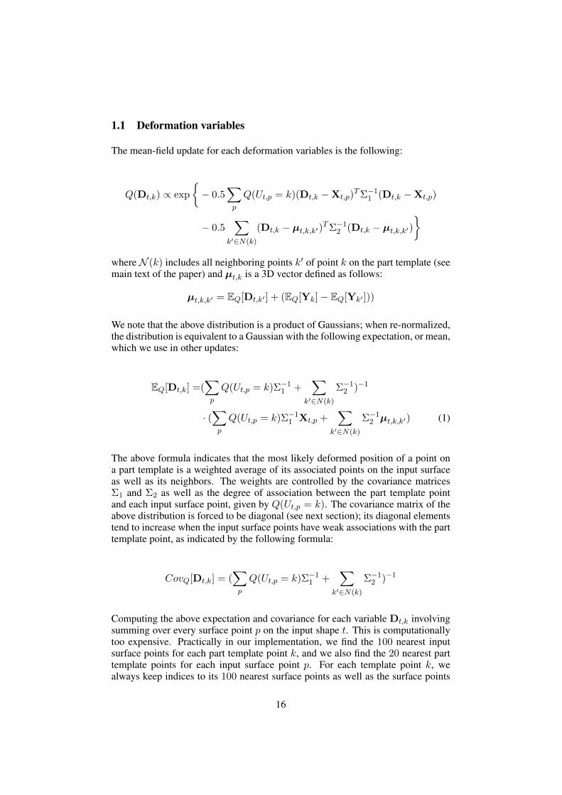
1.1 Deformation variables

The mean-field update for each deformation variables is the following:

Q(Dt,k) ∝ exp

{− 0.5

∑p

Q(Ut,p = k)(Dt,k −Xt,p)TΣ−11 (Dt,k −Xt,p)

− 0.5∑

k′∈N(k)

(Dt,k − µt,k,k′)TΣ−12 (Dt,k − µt,k,k′)

}

whereN (k) includes all neighboring points k′ of point k on the part template (seemain text of the paper) and µt,k is a 3D vector defined as follows:

µt,k,k′ = EQ[Dt,k′ ] + (EQ[Yk]− EQ[Yk′ ]))

We note that the above distribution is a product of Gaussians; when re-normalized,the distribution is equivalent to a Gaussian with the following expectation, or mean,which we use in other updates:

EQ[Dt,k] =(∑p

Q(Ut,p = k)Σ−11 +∑

k′∈N(k)

Σ−12 )−1

· (∑p

Q(Ut,p = k)Σ−11 Xt,p +∑

k′∈N(k)

Σ−12 µt,k,k′) (1)

The above formula indicates that the most likely deformed position of a point ona part template is a weighted average of its associated points on the input surfaceas well as its neighbors. The weights are controlled by the covariance matricesΣ1 and Σ2 as well as the degree of association between the part template pointand each input surface point, given by Q(Ut,p = k). The covariance matrix of theabove distribution is forced to be diagonal (see next section); its diagonal elementstend to increase when the input surface points have weak associations with the parttemplate point, as indicated by the following formula:

CovQ[Dt,k] = (∑p

Q(Ut,p = k)Σ−11 +∑

k′∈N(k)

Σ−12 )−1

Computing the above expectation and covariance for each variable Dt,k involvingsumming over every surface point p on the input shape t. This is computationallytoo expensive. Practically in our implementation, we find the 100 nearest inputsurface points for each part template point k, and we also find the 20 nearest parttemplate points for each input surface point p. For each template point k, wealways keep indices to its 100 nearest surface points as well as the surface points

16

whose nearest points include that template point k. Instead of summing over allthe surface points of each input shape, for each template point k we sum over itsabovementioned indices to surface point only. For the rest of the surface points,the distribution values Q(Ut,p = k) are practically negligible and are skipped inthe above summations.

1.2 Part template variables

For each part template point Yk, the mean-field update is given by:

Q(Yk) ∝ exp

{− .5(Yk − µk)

TΣ−12 (Yk − µk)

}where µk is the mean, or expectation (3D vector), defined as follows:

µk = EQ[Yk] =1

|N (k)|∑k′

(EQ[Yk′ ] +

1

T

∑t

(EQ[Dt,k]− EQ[Dt,k′ ]))

and N (k) includes all neighboring points k′ of point k on the part template, T isthe number of input shapes. The covariance matrix for the above distribution isgiven by Σ2.

1.3 Point correspondence variables

The mean-field update for the latent variables Ut,p yields a categorical distributioncomputed as follows:

Q(Ut,p = k) ∝ exp

{− 0.5(EQ[Dt,k]−Xt,p)

TΣ−11 (EQ[Dt,k]−Xt,p)

− 0.5Tr(Σ−11 · CovQ[Dt,k])

− 0.5(fk − ft,p)TΣ−13 (fk − ft,p)− ln ε ·Q(St,p = label(k))

}

where Tr(Σ−11 · CovQ[Dt,k]) represents the matrix trace, ε is a small constantdiscussed in the main text of the paper. For computational efficiency reasons, weavoid computing the above distribution for all pairs of part template and inputsurface points. As in the case of the updates for the deformation variables, we keepindices to input surface point positions that are nearest neighbors to part templatepoints and vice versa. We compute the above distributions only for pairs betweenthese neighboring points. For the rest of the pairs, we set Q(Ut,p = k) = 0.

17

1.4 Segmentation variables

The mean-field update for the variables St,p also yields a categorical distribution:

Q(St,p = l) ∝ exp

{∑k

Q(Ut,p = k)[label(k) 6= l] ln ε

+∑

p′∈N(p)

∑l′ 6=l

Q(St,p′ = l′) ln(1.0− Φ)

+∑

p′∈N(p)

Q(St,p′ = l) ln(Φ)

}

where N(p) is the neighborhood of the input surface point used for segmenta-tion (see main text for more details), Phi evaluates feature differences betweenneighboring surface points (see main text for its definition). The binary indicatorfunction [label(k) 6= l] is 1 if the expression in brackets holds, otherwise it is 0.

2 Covariance matrix updates

The covariance matrices of our factors are updated as follows:

Σ1 =1

Z1

∑t,k,p∈N (k)

Q(Ut,p = k)(EQ[Dt,k]−Xt,p)(EQ[Dt,k]−Xt,p)T

Σ2 =1

Z2

∑t,k,k′∈N(k)

((EQ[Dt,k]− EQ[Dt,k′ ])− (EQ[Yk]− EQ[Yk′ ]))·

· (EQ[Dt,k]− EQ[Dt,k′ ]− (EQ[Yk]− EQ[Yk′ ]))T

Σ3 =1

Z3

∑t,k,p∈N (k)

Q(Ut,p = k)(fk − ft,p)(fk − ft,p)T

Σ5 =1

Z5

∑t,p,p′∈N(p)

(ft,p − ft,p′)(ft,p − ft,p′)T

18

where Z1 = Z3 =∑

t,k,p∈N (k)

Q(Ut,p = k), Z2 =∑

t,k,k′∈N(k)

1, Z5 =∑

t,p,p′∈N(p)

1.

The computed covariance matrices are forced to be diagonal i.e., in the above com-putations only the diagonal elements of the covariance matrices are taken into ac-count, while the rest of the elements are set to 0.

3 Contrastive divergence

Contrastive divergence iterates over the following three steps in our implementa-tion: variational (mean-field) inference, stochastic approximation (or sampling),and parameter updates. We discuss the steps in detail below.

Variational inference step. Our deformation model yields expectations over de-formed point positions of the part templates based on Equation 1. For each de-formed point, we find the surface point that is closest to its expected position. LetDk,τ [t] the observed surface position of point k for an input shape t. The subscriptτ takes values 1, 2, or 3 that correspond to the x−,y−,z− coordinate of the pointrespectively. Let Ek[t] represents the observed existence of a point k (binary vari-able) also inferred by our deformation model. Given all observed point positionsD[t] and existences E[t] per shape t, we perform bottom-up mean-field inferenceon the binary hidden nodes according to the following equations in the followingorder:

Q(H(1)m = 1|D[t],E[t]) = σ

(wm,0 +

∑k∈Nm,τ

(ak,τ,m − ck,τ,m) ln(Dk,τ [t])Ek[t]

+∑

k∈Nm,τ(bk,τ,m − dk,τ,m) ln(1−Dk,τ [t])Ek[t]

+∑n

wm,nQ(H(2)n = 1|D[t],E[t])

)

Q(H(2)n = 1|D[t],E[t]) = σ

(wn,0 +

∑m

wm,nQ(H(1)m = 1|D[t],E[t])

+∑o

wn,oQ(H(3)o = 1|D[t],E[t])

)

Q(H(3)o = 1|D[t],E[t]) = σ

(wo,0 +

∑n

wn,oQ(H(2)n = 1|D[t],E[t])

)

where σ(·) represents the sigmoid function,Nm is the set of the observed variableseach hidden node (variable) H(1)

m is connected to. The mean-field updates for H(1)m

19

involve a weighted summation over the observed variables D[t] per part, whichcan be thought of as a convolutional scheme per part. We perform 3 mean-fielditerations alternating the updates over the above hidden nodes. During the firstiteration, we initialize Q(H

(2)n = 1) = 0 and Q(H

(3)o = 1) = 0 for each hidden

node n and o.

Stochastic approximation. This step begins by sampling the binary hidden nodesof the top layer for each training shape t. Sampling is performed according to theinferred distributions Q(H

(3)o = 1|D[t],E[t]) of the previous step. Let H(3)

o [t′] theresulting sampled 0/1 values. Then we perform top-down mean-field inference onthe binary hidden nodes of the other layers as well as the visible layer:

Q(H(2)n = 1|E[t],H(3)[t′]) = σ

(wn,0 +

∑m

wm,nQ(H(1)m = 1|E[t],H(3)[t′])

+∑o

wn,oH(3)o [t′]

)

Q(H(1)m = 1|E[t],H(3)[t′]) = σ

(wm,0 +

∑k∈Nm,τ

(ak,τ,m − ck,τ,m) ln(Dk,τ [t′])Ek[t]

+∑

k∈Nm,τ(bk,τ,m − dk,τ,m) ln(1−Dk,τ [t′])Ek[t]

+∑n

wm,nQ(H(2)n = 1|E[t],H(3)[t′])

)

Q(Dk,τ |E[t],H(3)[t′]) ∝

D

(ak,τ,0−1)+∑

m∈Nkak,τ,mQ(H

(1)m =1|E[t],H(3)[t′])+

∑m∈Nk

ck,τ,m(1−Q(H(1)m =1|E[t],H(3)[t′]))

k,τ

(1−Dk,τ )(bk,τ,0−1)+

∑m∈Nk

bk,τ,mQ(H(1)m =1|E[t],H(3)[t′])+

∑m∈Nk

dk,τ,m(1−Q(H(1)m =1|E[t],H(3)[t′]))

where Dk,τ [t′] in the above mean-field updates is set to be the expectation of theabove Beta distribution and Nk is the set of the hidden variables each observednode (variable) Dk,τ is connected to. We note that sampling all the variables in themodel caused contrastive divergence not to converge, thus we instead used expec-tations of the above distributions instead. As in the previous step, we performed 3iterations alternating over the above mean-field updates. During the first iteration,we skip the terms involvingDk,τ [t′] during the inference of the hidden nodes of thefirst layer. At the second and third iteration, we infer distributions for the hiddenlayers as follows:

Q(H(3)o = 1|D[t′],E[t]) = σ

(wo,0 +

∑n

wn,oQ(H(2)n = 1|D[t′],E[t])

)

20

Q(H(2)n = 1|D[t′],E[t]) = σ

(wn,0 +

∑m

wm,nQ(H(1)m = 1|D[t′],E[t])

+∑o

wn,oQ(H(3)o = 1|D[t′],E[t])

)

Q(H(1)m = 1|D[t′],E[t]]) = σ

(wm,0 +

∑k∈Nm,τ

(ak,τ,m − ck,τ,m) ln(Dk,τ [t′])Ek[t]

+∑

k∈Nm,τ(bk,τ,m − dk,τ,m) ln(1−Dk,τ [t′])Ek[t]

+∑n

wm,nQ(H(2)n = 1|D[t′],E[t])

)

Parameter updates. The parameters of the model are updated with project gra-dient ascent according to the expectations over the final distributions computed inthe previous two steps and the observed data. We list the parameter updates below.We note that sgn(·) used below denotes the sign function, ν is the iteration number(or epoch), η is the learning rate, µ is the momentum rate. The learning rate is setto 0.001 initially, and is multiplied by a factor 0.9 when at the previous epoch thereconstruction error

∑t,k,τ |Dk,τ [t]Ek[t]−Dk,τ [t′]Ek[t]| increases, and it is multi-

plied by a factor 1.1 when the reconstruction error decreases. The momentum rateis progressively increased from 0.5 towards 1.0 asymptotically during training.

ak,τ,0 = max(ak,τ,0 + ∆ak,τ,0[ν], 0) , where

∆ak,τ,0[ν] = µ ·∆ak,τ,0[ν − 1] + η1

T

∑t

(ln(Dk,τ [t])− ln(Dk,τ [t′])

)− ηλ1

∑k′∈Nk

sgn(ak,τ,0 − ak′,τ,0)− ηλ2sgn(ak,τ,0)

bk,τ,0 = max(bk,τ,0 + ∆bk,τ,0[ν], 0) , where

∆bk,τ,0[ν] = µ ·∆bk,τ,0[ν − 1] + η1

T

∑t

(ln(1−Dk,τ [t])− ln(1−Dk,τ [t′])

)− ηλ1

∑k′∈Nk

sgn(bk,τ,0 − bk′,τ,0)− ηλ2sgn(bk,τ,0)

21

ak,τ,m = max(ak,τ,m + ∆ak,τ,m[ν], 0) , where

∆ak,τ,m[ν] = µ ·∆ak,τ,m[ν − 1] + η1

T

∑t

(ln(Dk,τ [t])Q(H(1)

m = 1|D[t],E[t])

− ln(Dk,τ [t′])Q(H(1)m = 1|D[t′],E[t])

)− ηλ1

∑k′∈Nk

sgn(ak,τ,m − ak′,τ,m)− ηλ2sgn(ak,τ,m)

bk,τ,m = max(bk,τ,m + ∆bk,τ,m[ν], 0) , where

∆bk,τ,m[ν] = µ ·∆bk,τ,m[ν − 1] + η1

T

∑t

(ln(1−Dk,τ [t])Q(H(1)

m = 1|D[t],E[t])

− ln(1−Dk,τ [t′])Q(H(1)m = 1|D[t′],E[t])

)− ηλ1

∑k′∈Nk

sgn(bk,τ,m − bk′,τ,m)− ηλ2sgn(bk,τ,m)

ck,τ,m = max(ck,τ,m + ∆ck,τ,m[ν], 0) , where

∆ck,τ,m[ν] = µ ·∆ck,τ,m[ν − 1] + η1

T

∑t

(ln(Dk,τ [t])(1−Q(H(1)

m = 1|D[t],E[t])

− ln(Dk,τ [t′])(1−Q(H(1)m = 1|D[t′],E[t])

)− ηλ1

∑k′∈Nk

sgn(ck,τ,m − ck′,τ,m)− ηλ2sgn(ck,τ,m)

dk,τ,m = max(dk,τ,m + ∆dk,τ,m[ν], 0) , where

22

∆dk,τ,m[ν] = µ ·∆dk,τ,m[ν − 1] + η1

T

∑t

(ln(1−Dk,τ [t])(1−Q(H(1)

m = 1|D[t],E[t])

− ln(1−Dk,τ [t′])(1−Q(H(1)m = 1|D[t′],E[t])

)− ηλ1

∑k′∈Nk

sgn(dk,τ,m − dk′,τ,m)− ηλ2sgn(dk,τ,m)

wm,0 = wm,0 + ∆wm,0[ν] , where

∆wm,0[ν] = µ ·∆wm,0[ν − 1] + η1

T

∑t

(Q(H(1)

m = 1|D[t],E[t])

−Q(H(1)m = 1|D[t′],E[t])

)− ηλ2sgn(wm,0)

wn,0 = wn,0 + ∆wn,0[ν] , where

∆wn,0[ν] = µ ·∆wn,0[ν − 1] + η1

T

∑t

(Q(H(2)

n = 1|D[t],E[t])

−Q(H(2)n = 1|D[t′],E[t])

)− ηλ2sgn(wn,0)

wo,0 = wo,0 + ∆wo,0[ν] , where

∆wo,0[ν] = µ ·∆wo,0[ν − 1] + η1

T

∑t

(Q(H(3)

o = 1|D[t],E[t])

−Q(H(3)o = 1|D[t′],E[t])

)− ηλ2sgn(wo,0)

23

wm,n = wm,n + ∆wm,n[ν] , where

∆wm,n[ν] = µ ·∆wm,n[ν − 1] + η1

T

∑t

(Q(H(1)

m = 1|D[t],E[t])Q(H(2)n = 1|D[t],E[t])

−Q(H(1)m = 1|D[t′],E[t])Q(H(2)

n = 1|D[t′],E[t])

)− ηλ2sgn(wm,n)

wn,o = wn,o + ∆wn,o[ν] , where

∆wn,o[ν] = µ ·∆wn,o[ν − 1] + η1

T

∑t

(Q(H(2)

n = 1|D[t],E[t])Q(H(3)o = 1|D[t],E[t])

−Q(H(2)n = 1|D[t′],E[t])Q(H(3)

o = 1|D[t′],E[t])

)− ηλ2sgn(wn,o)

3.1 Parameter updates for the structure part of the BSM

To learn the parameters wk,0, wk,r, wr,0 involving the variables E and G of theBSM part modeling the shape structure, we similarly perform contrastive diver-gence with the following steps:

Inference. Given the observed point existences E[t], we infer the following distri-bution over the latent variables G (we note that this is exact inference):

Q(Gr = 1|E[t]) = σ(wr,0 +∑k

wk,rEk[t])

Sampling. We sample the binary latent variables G according to the inferred distri-bution Q(Gr = 1|E[t]). Let Gr[t′] the resulting sampled 0/1 values. We performinference for the existence variables as follows:

Q(Ek = 1|G[t′]) = σ(wk,0 +∑r

wk,rGr[t′])

24

and repeat for the latent variables:

Q(Gr = 1|G[t′]) = σ(wr,0 +∑k

wk,rQ(Ek = 1|G[t′]))

Parameter updates The parameters of the structure part of the BSM are updatedas follows:

wk,0 = wk,0 + ∆wk,0[ν] , where

∆wk,0[ν] = µ ·∆wk,0[ν − 1] + η1

T

∑t

(Ek[t]−Q(Ek = 1|G[t′])

)− ηλ1

∑k′∈Nk

sgn(wk,0 − wk′,0)− ηλ2sgn(wk,0)

wr,0 = wr,0 + ∆wr,0[ν] , where

∆wr,0[ν] = µ ·∆wr,0[ν − 1] + η1

T

∑t

(Q(Gr = 1|E[t])−Q(Gr = 1|G[t′])

)− ηλ2sgn(wr,0)

wk,r = wk,r + ∆wk,r[ν] , where

∆wk,r[ν] = µ ·∆wk,r[ν − 1] + η1

T

∑t

(Ek[t]Q(Gr = 1|E[t])

−Q(Ek = 1|G[t′])Q(Gr = 1|G[t′])

)− ηλ1

∑k′∈Nk

sgn(wk,r − wk′,r)− ηλ2sgn(wk,r)

References

[1] Daphne Koller and Nir Friedman. Probabilistic Graphical Models: Principlesand Techniques. The MIT Press, 2009.

25

Analysis and synthesis of 3D shape families viadeep-learned generative models of surfaces

User Study

We conducted a perceptual evaluation of our synthesized shapes with volunteers re-cruited through Amazon Mechanical Turk. Each volunteer performed 40 pairwisecomparisons in a web-based questionnaire. Each comparison was between imagesof two shapes from the chairs or airplanes domain. For each pair, one shape wascoming from the training collection of one of the two domains, and the other shapewas coming from our collection of synthesized shapes of the same domain. Thetwo shapes were randomly sampled from their collections. They appeared in arandom order on the web pages of the questionnaire.

The participants were asked to choose which of the two presented shapes was moreplausible, or indicate whether they found both shapes to be equally plausible, ornone of them to be plausible. Each questionnaire contained 20 unique compar-isons and each comparison was repeated twice by flipping the order of the twoshapes in the question. To diminish the risk of contaminating the results of the userstudy with unreliable respondents, we excluded participants that gave two differentanswers to more than 6 of the 20 unique comparisons, or took less than 2 minutesin total to complete the questionnaire.

The number of reliable Mechanical Turk respondents after the above filtering was31. A total of 1240 pairwise comparisons were gathered in total. The resultsare visualized in the following figure. The user study indicates that the shapesproduced by our model were seen as plausible as the training shapes of the inputcollection.

195 votes: 210 votes: 171 votes:32 votes:synthesized airplanes

are more plausibleboth airplanes are plausible

none areplausible

training airplanesare more plausible

148 votes: 260 votes: 163 votes:61 votes:synthesized chairsare more plausible

both chairs are plausible

none areplausible

training chairsare more plausible

Figure 1: Results of our Amazon Mechanical Turk user study

26

analysis and synthesis of 3d shape families via deep

Documents