analysis and testing of a lidar-based approach to … institute of aeronautics and astronautics 1...

American Institute of Aeronautics and Astronautics

1

Analysis and Testing of a LIDAR-Based Approach to Terrain Relative Navigation for Precise Lunar Landing

Andrew E. Johnson1 and Tonislav I. Ivanov2 Jet Propulsion Laboratory, California Institute of Technology, 4800 Oak Grove Drive, Pasadena, CA, 91109

To increase safety and land near pre-deployed resources, future NASA missions to the moon will require precision landing. A LIDAR-based terrain relative navigation (TRN) approach can achieve precision landing under any lighting conditions. This paper presents results from processing flash lidar and laser altimeter field test data that show LIDAR TRN can obtain position estimates less than 90m while automatically detecting and eliminating incorrect measurements using internal metrics on terrain relief and data correlation. Sensitivity studies show that the algorithm has no degradation in matching performance with initial position uncertainties up to 1.6 km.

Nomenclature ALHAT = Autonomous Landing and Hazard Avoidance Technology LIDAR = Light Detection And Ranging TRN = terrain relative navigation DEM = digital elevation map NTS = Nevada Test Site DV = Death Valley USGS = United States Geological Survey UTM = Universal Transverse Mercator ECEF = Earth Centered Earth Fixed Frame CEP 95% = Circular Error Probable 95% Radius CEP 99% = Circular Error Probable 99% Radius V/CNF = Valid Over Confident Fraction V/COR = Valid Over Correct Fraction P2V = Peak-to-Valley TRI = Terrain Relief Index

I. Introduction RECISE landing on the surface of the Moon is the goal for future lunar missions of NASA. Such capability will enable scientists to get closer to a point of interest and to access rougher terrain. However, traditional lunar

landing approaches, based on inertial sensing, do not have the navigational precision to meet this goal. To address this shortcoming, several terrain relative navigation (TRN) approaches have been proposed.1-6 These approaches sense the terrain during descent and augment the inertial navigation by providing, in real-time, position or bearing estimates relative to known surface landmarks. From these estimates, the navigational precision can be increased to a level that meets a requirement of landing within 90 m of a predetermined location.7

The Autonomous Landing and Hazard Avoidance Technology (ALHAT) project of NASA is developing a LIDAR-based terrain relative navigation algorithm.8-10 Unlike other algorithms, this is an active range sensing approach that can operate under any illumination conditions and can enable landing anywhere on the Moon at any time of day. The proposed TRN approach is intended for use during the braking burn phase of a lander, after it de-orbits. During this phase, the lander travels a significant distance downrange at a shallow path angle; thus, the cumulative LIDAR data forms a long contour. Additionally, the LIDAR can be placed on a single-axis gimbal that swings in the cross-track direction to produce a wider contour. After collection, the LIDAR data is projected into a

1 Supervisor GN&C Hardware and Testbed Development Group, MS 301-121, AIAA member 2 Associate Member of Technical Staff, Computer Vision Group, MS 198-236

P


2

digital elevation map (DEM) using the most current position estimate for the lander. To obtain a position correction, this “LIDAR DEM” is correlated with a “reference DEM” constructed from a-priori reconnaissance, such as the Lunar Reconnaissance Orbiter data. High-fidelity simulation of the LIDAR TRN has shown that both regular and wide contours can achieve the ALHAT 90 m precision objective.1

This paper describes the performance of the LIDAR-based TRN approach using data collected during a recent field test described in section II. More detail on the algorithm is given in section III. The approach produces position estimates and associated confidence using internal metrics introduced in section IV. In most field test flights, as shown in section V, the confident estimates have error typically less than 90 m. Misalignments are the likely causes of the large position errors in other flights. In addition, in Section VI, studies were conducted to assess the sensitivity to confidence metric, contour length, map pixel size, and initial position uncertainty.

II. Field Test Description To further mature LIDAR TRN, as well as other TRN approaches, ALHAT conducted a field test in June and

July of 2009. For this test, a fixed-wing aircraft was outfitted with a suite of TRN sensors, along with sensors to provide ground truth position and attitude. A gimbaled platform contained two laser ranging sensors: a flash LIDAR collected multiple ranges for each image acquired while a laser altimeter provided one range but at a faster rate than the flash LIDAR. The gimbal had different modes to obtain a variety of contour widths. Details on the field test implementation, platform, and ground truth trajectory generation can be found in [Keim 2010]12. A total of eight data collection flights were flown. For most flights, the plane flew horizontally at 60 m/s. The flights were conducted at 2, 4, and 8 km altitudes over two test sites: Death Valley (DV) and Nevada Test Site (NTS). A variety of terrain was imaged including mountains, hills, washes, dry lakebeds, and craters. Each flight had between one and two hours of valid data.

NTS and DV were selected as test sites for the field test because of the lack of vegetation over large areas and the variety of terrain relief. NTS in particular was selected because it has a large crater field on a flat terrain, analogous to the lunar mare. DV in particular was selected because of the mountainous regions and associated foothills that are analogous to the lunar uplands.

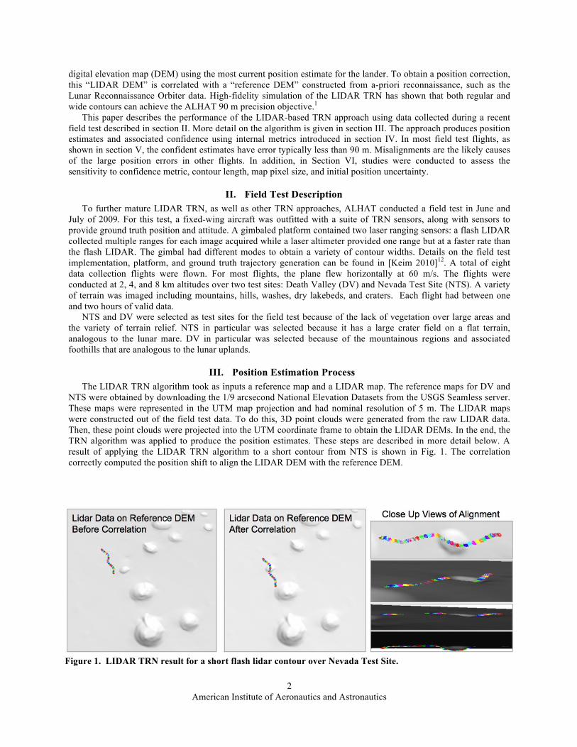
III. Position Estimation Process The LIDAR TRN algorithm took as inputs a reference map and a LIDAR map. The reference maps for DV and

NTS were obtained by downloading the 1/9 arcsecond National Elevation Datasets from the USGS Seamless server. These maps were represented in the UTM map projection and had nominal resolution of 5 m. The LIDAR maps were constructed out of the field test data. To do this, 3D point clouds were generated from the raw LIDAR data. Then, these point clouds were projected into the UTM coordinate frame to obtain the LIDAR DEMs. In the end, the TRN algorithm was applied to produce the position estimates. These steps are described in more detail below. A result of applying the LIDAR TRN algorithm to a short contour from NTS is shown in Fig. 1. The correlation correctly computed the position shift to align the LIDAR DEM with the reference DEM.

Figure 1. LIDAR TRN result for a short flash lidar contour over Nevada Test Site.


3

A. Generating 3D Point Clouds The flash LIDAR data consisted of 128 by 128 pixel images. Each pixel in a LIDAR image consisted of 20

timed intensities of the return laser pulse. First of all, pixels that constantly yielded erroneous readings or did not trigger, i.e. did not register a reading, were disregarded. Next, the maximum intensity for each remaining pixel was determined by finding the peak of a 6th order polynomial fit to the timed return pulse intensities. The corresponding time-of-flight for this maximum, as measured by the LIDAR’s clock, was then multiplied by the speed of light over two to yield a range for that pixel. Also, the ranges were calibrated to deal with drifting clock rate and pixel-to-pixel non-uniformities. Additionally, to remove any remaining outliers, a local median filter was applied to the ranges. Finally, a 3D point cloud was generated for each image by computing the rays for each pixel using a perfect perspective camera projection. For the laser altimeter sensor, a single range is measured each time the laser is fired. This range along the known sensor boresight is turned into a single 3D point for each altimeter measurement.

B. Constructing the LIDAR DEM The 3D point clouds were represented in the LIDAR sensor coordinate frame. They needed to be transformed

into the UTM frame to generate a LIDAR DEM with the same frame as that of the reference map. Beforehand, a flight trajectory was computed that defined the position and attitude of the LIDAR in the Earth Centered Earth Fixed Frame (ECEF). This trajectory was interpolated to construct rigid transformations that, at each LIDAR image instance, mapped the sensor frame to the ECEF. Next, the 3D point cloud for each image was transformed into the ECEF, then into latitude/longitude/height, and finally into the UTM frame. After 3D point clouds from several sequential LIDAR images were transformed into the UTM frame, the new points were inserted into a two dimensional map array using bilinear interpolation to form the LIDAR contour DEM10. The LIDAR DEM resolution was set to 5 m to match the one of the reference DEM. The width of the LIDAR contour depended on whether the gimbal was moving or not during flight. The length of the contour depended on the number of images used to form it and was adjusted to tune the performance.

C. Correlating the DEMs The bounds of the LIDAR DEM, increased by the position uncertainty of 200 m, were used to crop the large

reference DEM. The LIDAR DEM and the cropped reference DEMs were matched using a floating-point correlation algorithm13 that handled missing data. The maximum value in the correlation map resulting from the algorithm corresponded to the horizontal shift between the contour and the reference DEM. To increase the precision of this shift, a bi-quadratic fit was made to a neighborhood around the correlation peak to compute a sub-pixel maximum. This shift in pixels was converted to a shift in meters using the DEM pixel size. The process described above was automated and all flights were processed at nominal parameters. Additionally, studies were conducted on a smaller subset to determine sensitivity to driving parameters.

IV. Analysis Metrics

A. Performance Metrics The purpose of TRN was to provide accurate position estimates. The error of an estimate was determined by the

difference between the position estimated by the algorithm and the position computed from the ground truth data. Recall that the ALHAT requirement was to land within 90 m horizontal distance of the intended landing point. Thus, for the purpose of this analysis, a position estimate was labeled “correct” if it had a position error less than 90 m. An incorrect estimate was one that had a position error greater than 90 m.

In addition to estimating position, the TRN algorithm established a level of confidence for the estimates. As described below, this was done by applying thresholds to three metrics internal to the algorithm in such a way that the estimates satisfy the thresholds had high accuracy. An estimate that satisfied all thresholds was labeled as “confident,” and were passed by the algorithm to the navigation filter. Estimates that were both correct and confident are dubbed as “valid” and those that were incorrect and confident – as “invalid.” Four metrics were used to describe position estimation performance:

• Valid Over Correct Fraction (V/COR): The number of valid (correct and confident) estimates over the total number of correct estimates. This metrics describes the percentage of the correct estimates that are marked as confident.

• Valid Over Confident Fraction (V/CNF): The ratio of the number of valid (correct and confident) estimates over the number of all confident estimates. This metrics describes the percentage of the confident estimates passed on to navigation that are correct.


4

• CEP 95%: The circular error probable radius (in meters) centered on (0,0) meters containing 95% of the confident position estimates. CEP is an error metric common in targeting applications.

• CEP 99%: The circular error probable radius (in meters) centered on (0,0) meters containing 99% of the confident position estimates.

B. Confidence Metrics Metrics were developed to assign a measure of confidence to the TRN position estimates and also decided which

estimates can be used in navigation. Without these confidence metrics the TRN algorithm could pass estimate with large errors. The aim was to achieve the greatest number of correct estimates, while allowing very few incorrect estimates, to be passed on to navigation.

The correlation peak height, correlation peak width, and peak ratio were output as correlation metrics. These metrics were computed after the algorithm was run and described properties of the correlation DEM matching procedure done by TRN. Additionally, four terrain metrics were calculated from the LIDAR contour. These metrics were computed from the LIDAR data and describe properties of the terrain contour used in TRN matching. It was supposed that the terrain relief and the geometry of the contour related to the TRN error. All terrain metrics were computed locally, on a sliding 100 m by 100 m window, and then the overall maximum result for the contour was taken. Multiple TRN confidence metrics were investigated, and the ones in bold were most discriminative of correct and incorrect estimates. These are to be used inside the sensor to label confidence.

• Correlation peak height (unitless, between -1 and 1) – the height of the correlation peak. Height is defined as the distance from the (x,y) plane to the vertex of the bi-quadratic fit around the peak.

• Correlation peak width (pixels) – the maximum width of the correlation peak. Width is determined as the major radius of the ellipse formed by the intersection of the biquadratic and the (x,y) plane.

• Peak ratio (unitless) – the ratio in heights of the correlation peak and the second highest peak. The second highest peak is the peak with the next highest correlation height.

• Peak-to-Valley (meters) – the difference between the highest and the lowest elevation in the terrain contour after it is projected on the median plane to remove the effect of overall slope.

• Terrain Relief Index (TRI) (meters) – the expected standard deviation of elevations among neighboring pixels.11

• Contour size (pixels) – the total number of DEM pixels in the contour. • Contour shape (unitless) – a measure of length and width of the contour as described by the two eigenvalues

of the scatter matrix of the x and y coordinates of the contour points. An estimate was labeled “confident” if the three metrics in bold above satisfied respective thresholds:

(Correlation Peak height > 0.7) and (Correlation Peak Width < 70 pixels) and (Peak To Valley > 10 meters) The aim of the confidence metrics is to have the highest number of valid estimates, while maintaining a very low

number of incorrect and confident estimates. Loosening the thresholds allows a greater number of valid estimates to be obtained. However, the average error of these estimates increases and also more incorrect estimates are passed. Vice versa, tightening the thresholds results in a significant number of valid estimates to be thrown out in order to achieve the lowest possible number of confident and incorrect estimates. Thus, we traded off higher confidence in the confident estimates for lesser number of valid estimates.

V. Performance Analysis of Flights: Flash LIDAR data Based on the contour length sensitivity study describe in the next section, 75 consecutive flash LIDAR images

were used to construct each contour in every flight. Given the 10 Hz rate of the LIDAR and the 60 m/s speed of the aircraft, this resulted in contour length of 450m. The processing steps, described in Section III, were applied to each contour and the TRN position correction was recorded along with all the confidence metrics mentioned above. Since the ground truth trajectory was used to transform the LIDAR samples into the map frame, the position correction should have been zero; thus, the computed correction was actually the error in position estimation. However, the ground truth had noticeable biases in some flights.

Table 1 summarizes the performance metrics for all flights. To further illustrate the performance of the LIDAR TRN algorithm, scatter plots of the horizontal position errors are shown in Fig. 2. The four possible labels for a TRN position measurement were marked as fallows:

• Confident and correct (green dot) • Confident and incorrect (red dot) • Not confident and correct (cyan circle) • Not confident and incorrect (blue dot)


5

The performance for flights 2, 3, 4, 5, and 7 was very good. The errors on the confident measurements are clustered near zero and the CEP 95% was less than 90m. Flights 4, 5, 7 were at NTS and had CEP 99% less than 90m. Flights 2 and 3 were at DV and had CEP 99% over 90m due to a few large outliers (red dots), which would likely be thrown out by the navigation filter that is the recipient of the TRN measurements. The high V/CNF percentage indicates that the confidence metrics are doing a good job of separating the correct measurements from the incorrect measurements; thus, most estimates passed on to navigation were actually correct. Also, a large number of the correct estimates were retained by the metrics as indicated by the V/COR percentage.

Flight 1 has the worst performance. The scatter plot indicates a possible cause for the poor performance. The off center clustering suggests an unknown and constant misalignment from the ground truth trajectory. Since attitude is

Figure 2. TRN performance for all flights with LIDAR data. These plots show the distribution of error for the TRN position estimates across flights. For most flights, the confident estimates (solid dots) are green, i.e. within the 90 m requirement (dotted circle). The system detects and discards a lot of its erroneous estimates (blue circles).

Table 1. Comparison of position estimation performance

Flash LIDAR Laser Altimeter

V/COR (%)

V/CNF (%)

CEP 95% (m)

CEP 99% (m)

V/COR (%)

V/CNF (%)

CEP 95% (m)

CEP 99% (m)

D V

1 87.4 79.1 125.7 144.0 212 93 98.7 118.8 2 77.7 96.8 65.2 100.3 215 98.2 66.9 100.2 3 91.3 98.1 51.0 141.4 - - - - 8 - - - - - - - -

N T S

4 68.3 98.8 37.0 77.7 222 98.2 26.2 97.1 5 64.2 99.7 31.0 56.9 282 98.3 34.3 133.8 6 - - - - - - - - 7 58.8 100 30.2 42.9 132 99.2 42.3 58.2


6

assumed perfect, errors in pointing will be compensated by errors in estimated position. Another possible source of the error is the narrower 5x divergence (i.e., beam width) on the flash lidar laser used on Flight 1 (and Flight 3) relative to Flights 2, 4, 5 and 7. To obtain greater maximum range the divergence of the transmit laser was decreased. This narrowing resulted in about 100 triggering pixels per image when the plane was at 2 km altitude and 50 or fewer at higher altitude. In Flights 2, 4, 5, and 7 the wider 2x divergence was used, which resulted in 400 pixels at 2 km and 200 pixels at 4 km altitude. This difference meant that the LIDAR contours for Flights 1 and 3 were narrower than those of the other flights , which could explain the greater spread in error.

Flights 6 and 8 had apparent large ground truth trajectory errors. These flights were the last ones performed after a week of down time for the aircraft during which some work was done on the sensors. This may have effected the alignment of the LIDAR and LA with the rest of the system. Additionally, during Flight 8, the LIDAR had problems outputting its clock rate, making it impossible to calibrate the range and make accurate LIDAR maps.

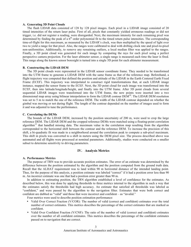
Fig. 3 shows the magnitude of the horizontal error plotted against the three confidence metrics for Flight 2. In each plot the threshold used is shown as a black line. Peak to valley is the best metric for separating correct from incorrect estimates. Correlation peak height and peak width help eliminate a few more incorrect estimates as indicated by the blue circles above the peak to valley threshold on the left plot in Fig 3. The position estimation results for Flight 2 were plotted on a contour map of DV in Fig. 6. One can see that most errors occurred in the flat portions of the terrain, whereas most correct estimates were over the rougher terrain. Therefore, the performance of LIDAR TRN is driven by the amount of terrain relief present in the LIDAR data.

VI. Performance Analysis of Flights: Laser Altimeter data In each flight, Laser Altimeter (LA) data was collected along with flash LIDAR data. For comparative purposes,

the LA segments were matched to cover the same area as the flash LIDAR segments. Since both instruments were aligned and timed the same, we calculated the start and end time of each 7.5 sec LIDAR segment and then extracted the corresponding LA data. A range correction of 42 m was added to all LA ranges to account for a known constant bias in range. Furthermore, outlier ranges were eliminated. The LA had sparsely spaced points in each segment, and much fewer points than flash LIDAR. These LA 3D point clouds were turned into a DEM following the procedure of section III.B and matched to the reference DEM using the TRN algorithm tolerant to sparse/missing data as described in section III.C.

To analyze the LA performance, the same metrics were used as in sections IV. Scatter plots were made of horizontal position error (Fig. 4). The laser altimeter did not produce results for Flight 3, 6, or 8.

Table 1 above summarizes numerically the performance results of the LA. All successful flights (1,2,4,5,7) had most errors clustered near (0,0) and CEP95% < 90m. The DV flights (1,2) had larger errors than the NTS flights (4,5,7), which may be due to the better quality of map for the NTS site.

By looking at flash LIDAR and LA results in Tables 1 one can see that the LA performed almost as well as flash LIDAR despite having much fewer samples. This proves that the TRN elevation correlation algorithm works robustly even on terrain with a few significant features (i.e. with peak-to-valley 10 m). The errors from the LA and LIDAR contours were correlated. Comparing the error distributions over the test site maps (Fig. 6) shows that both data sets gave very similar performance over the same terrain – good results for rough terrain and bad for flat.

Figure 3. TRN metrics for Flight 2 with LIDAR data. These plots show the metric value versus the error for the TRN position estimates. Acceptable estimates are to the left of the vertical line marking the 90m error. The horizontal lines are the metric thresholds.


7

VII. Sensitivity Studies In addition to processing the LIDAR data from all flights, studies were conducted to assess the sensitivity to

confidence metric, contour length, map pixel size, and initial position uncertainty. Because of its relatively good performance, Flight 2 was used in these studies.

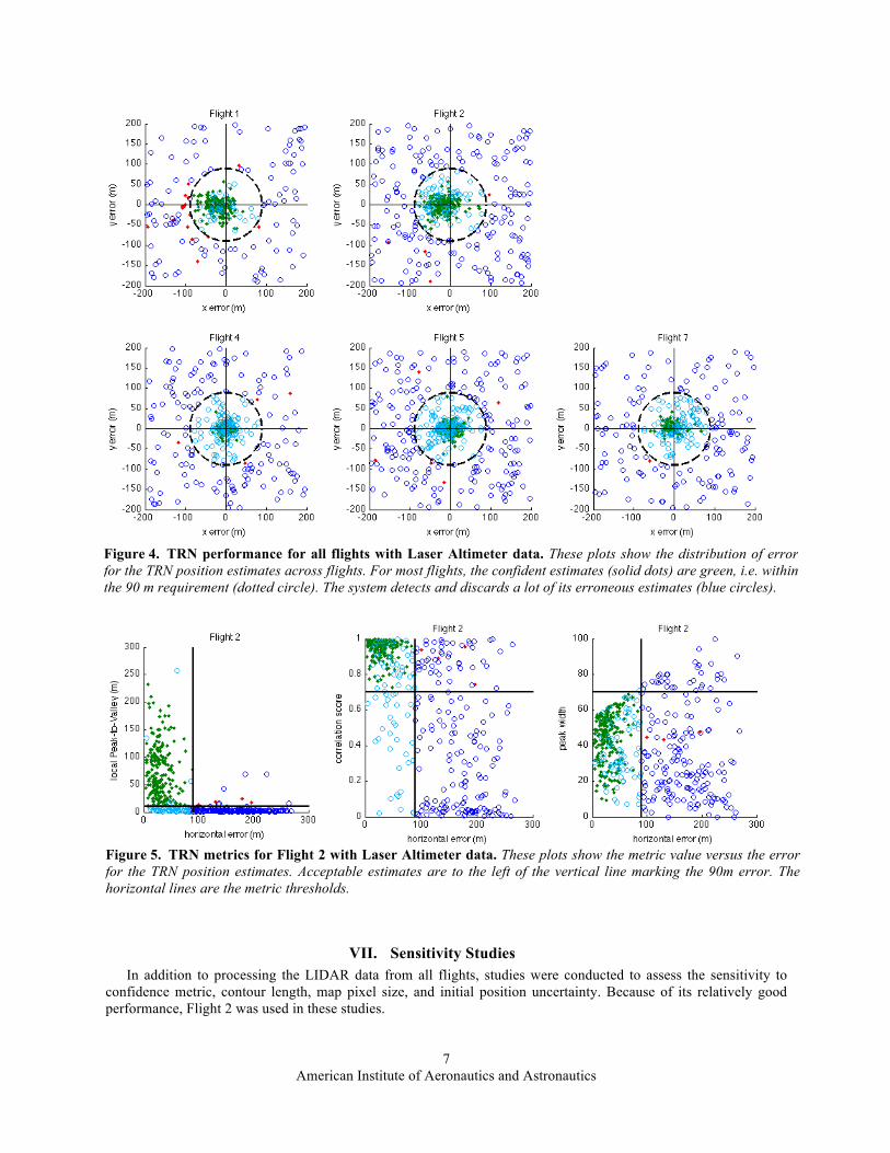
Figure 5. TRN metrics for Flight 2 with Laser Altimeter data. These plots show the metric value versus the error for the TRN position estimates. Acceptable estimates are to the left of the vertical line marking the 90m error. The horizontal lines are the metric thresholds.

Figure 4. TRN performance for all flights with Laser Altimeter data. These plots show the distribution of error for the TRN position estimates across flights. For most flights, the confident estimates (solid dots) are green, i.e. within the 90 m requirement (dotted circle). The system detects and discards a lot of its erroneous estimates (blue circles).


8

A. Confidence Metric Study After observing plots, such as those in Fig. 3, for all confidence metrics, it was found out that P2V and TRI were

the best metrics. Almost all estimates above their respective thresholds (25 m for P2V and 1 m for TRI) were correct. Both of these metrics describe terrain relief and utilize the fact that higher relief results in better estimates.

The contour size and shape did not have an observable relation with the error. This confirmed the intuition that it was only necessary to have one unique feature in the contour to lock in the correlation. Also, if the contour had no features and was flat, its shape did not improve error.

The correlation peak height, peak width, and peak ratio were able to throw out estimates with high error, which occurred because of very flat terrain that was hard to match. However, these metrics were mostly subsumed by the P2V and the TRI metrics.

B. Contour Length Study This study aimed to determine the contour length that generated the highest total number of valid estimates as

determined by the confidence metrics. Five sets of contours were generated with different lengths using: 600, 300, 150, 75, and 37 images. Note that 600 images represent 60 s of data and about 3600 m of flight path.

As the number of images in the segments decreased, the TRN updates became more frequent; thus, the total number of estimates increased. It was observed that the total number of valid estimates detected by the metrics also increased, giving a higher rate of confident estimates passed on to navigation. However, the marginal increase became smaller every time the length was cut in half. Also, the error of the valid estimates increased by a few meters. Furthermore, confident but incorrect estimates started appearing. Therefore, the number of valid estimates increased, but the quality of these estimates degraded with shorter segment length. The contour length with 75 images maximized the number of valid estimates while keeping the confident and incorrect estimates to a minimum.

! !

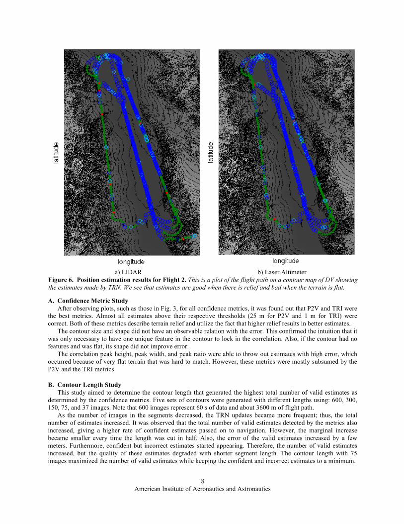
a) LIDAR b) Laser Altimeter

Figure 6. Position estimation results for Flight 2. This is a plot of the flight path on a contour map of DV showing the estimates made by TRN. We see that estimates are good when there is relief and bad when the terrain is flat.


9

C. Map Pixel Size Study The LIDAR TRN algorithm is based on correlation between a LIDAR DEM and a reference DEM. As the size

of the pixels in the map increases the accuracy of the peak fit during correlation decreases and, consequently, the position estimates become less accurate. To assess the sensitivity to map pixels size flights 2 and 7 were used.

As seen in the left plot of Fig. 7, the mean error of the valid position estimates increased as the map pixel size increased. There was a linear growth in the mean error when pixel size was between 20 and 80 m. However, there was essentially no change in error when resolution was between 5 and 20 m. This discrepancy was likely due to an error in the ground truth on the order of 20 m, which caused the constant estimate error despite change in resolution. Also, Flight 2 over DV initially had twice as much error as Flight 7 over NTS. This was probably due to the ground truth error being larger for DV than NTS.

As seen in the right plot of Fig. 7, the percentage of confident estimates that are incorrect increased as the map pixel size increased. The terrain relief was being smoothed as map resolution increased. With less terrain relief, the contours became less unique, which increased the chance of incorrect matches.

0

20

40

60

80

100

0 200 400 600 800 1000 1200 1400 1600

me

an

ho

rizo

nta

l p

ositio

n e

rro

r (m

)

position uncertainty radius (m)

Valid and Correct Mean Error(map resolution = 5m)

DV flight2 450m contoursDV flight2 225m contours

NTS flight7 450m contoursNTS flight7 225m contours

0

0.2

0.4

0.6

0.8

1

0 200 400 600 800 1000 1200 1400 1600

ratio

position uncertainty radius (m)

Incorrect Over Valid Fraction(map resolution = 5m)



a) Valid mean error b) Invalid over confident Figure 8. Position uncertainty sensitivity study.

0

20

40

60

80

100

0 20 40 60 80 100

mean h

orizonta

l positio

n e

rror

(m)

map pixel size (m)

Valid and Correct Mean Error(Position Uncertainty=200m)



0

0.2

0.4

0.6

0.8

1

0 20 40 60 80 100

ratio

map pixel size (m)

Incorrect Over Valid Fraction(Position Uncertainty=200m)



a) Valid mean error b) Invalid over confident

Figure 7. Map pixel size sensitivity study.


10

D. Position Uncertainty Study Plots of the performance metrics as a function of the position uncertainty for Flights 2 and 7 are show in Fig. 8.

The valid mean error and the invalid over confident fraction did not change with uncertainty. Therefore, the LIDAR TRN algorithm is not sensitive to the position uncertainty and could easily handle the initial position uncertainties of about 1 km expected during lunar landing. However, as the position uncertainty increased, the size of the correlation search area increased, and so did the computation time of the algorithm.

VIII. Conclusion The TRN approach presented here, based on correlation of LIDAR data and an elevation map, meets the

objective of 90 m landing precision under any lighting conditions. In our experiments with field test data, TRN estimates had error typically less than 50 m. Most incorrect estimates are eliminated using confidence metrics based on terrain relief and correlation statistics. Instrument misalignments were the main causes of large global errors. Disregarding those, more than 95% of the TRN estimates passed on to the navigation filter were accurate. Furthermore, the algorithm was able to handle initial position uncertainty of 1.6 km without performance degradation. However, TRN performance degraded with larger map pixel sizes.

Future work will include a study of the effect of contour width on TRN performance. Also, pre-filtering of the contours though a band-pass filter or masking out flat regions will be investigated to sharpen the correlation peak.

Acknowledgments The work described in this publication was performed at the Jet Propulsion Laboratory, California Institute of

Technology, under contract from the National Aeronautics and Space Administration. The authors would like to thank the entire ALHAT Field Test 3 Team at JPL and the lidar sensor developers at NASA Langley Research Center. This work was performed under the ALHAT Project managed by NASA Johnson Space Center and funded by the NASA Exploration Technology Development Program.

References 1Johnson, A., and Montgomery, J., “Overview of Terrain Relative Navigation Approaches for Precise Lunar Landing,” Proc.

of the IEEE Aerospace Conference, Big Sky, MT, 2008. 2Aggarwal, J., and Sabata, B., “Estimation of Motion from a Pair of Range Images: A Review,” Computer Vision, Graphics,

and Image Processing, Vol. 54, No. 3, 1991, pp. 309-324. 3Shah, M. and Kumar, R., (eds.), Video Registration, Kluwer Academic Publishers, Boston, 2003, Chapter 7 “Geodetic

Alignment of Aerial Video Frames,” by Sheikh, Y., Khan, S., Shah, M., and Cannata, R. 4Gaskell, R., “Automated Landmark Identification for Spacecraft Navigation,” Proc. of the AAS/AIAA Astrodynamics

Specialists Conference, 2001. 5Cheng, Y., and Ansar, A., “Landmark Based Position Estimation for Pinpoint Landing on Mars,” Proc. of the IEEE Int’l

Conf. on Robotics and Automation (ICRA), Barcelona, Spain, 2005, pp. 4470–4475. 6Johnson, A. et al., “A General Approach to Terrain Relative Navigation for Planetary Landing”, Proc. the AIAA Infotech at

the Aerospace Conference, Rohnert Park, CA, 2007. 7Epp, C. and Smith, T., “The Autonomous Precision Landing and Hazard Detection and Avoidance Technology (ALHAT),”

Proc. of the Aerospace Conference, Big Sky, MT, March 2008, pp. 1-7. 8Golden, J. P., “Terrain Contour Matching (TERCOM): a Cruise Missile Guidance Aid,” Image Processing for Missile

Guidance, Proc. of the Society of Photo-optical Instrumentation Engineers, Vol. 238, 1980, pp. 10-18. 9Carr, J. C., and Sobek, J. L., “Digital Scene Matching Area Correlator (DSMAC),” Image Processing for Missile Guidance,

Proc. of the Society of Photo-Optical Instrumentation Engineers, Vol. 238, 1980, pp. 36-41. 10Johnson, A., and SanMartin, M., “Motion Estimation from Laser Ranging for Autonomous Comet Landing,” Proc. of the

Int'l Conf. on Robotics and Automation (ICRA), San Francisco, CA, 2000, pp. 132-138. 11Riley, S., DeGloria, S., and Elliot, R., “A Terrain Ruggedness Index That Quantifies Topographic Heterogeneity,”

International Journal of Science, Vol. 5, No. 1-4, 1999, pp. 23-26. 12Keim, J., “Field Test Implementation to Evaluate a Flash Lidar as a Primary Sensor for Safe Lunar Landing,” Proc. of the

Aerospace Conference, Big Sky, MT, March 2010, paper 2.0304. 13 Lewis, J.P., “Fast Template Matching,” Vision Interface, Quebec City, CA, May 15-19 1995, pp. 120–123.

analysis and testing of a lidar-based approach to … institute of aeronautics and astronautics 1...

Documents