NASA Technical Memorandum 4174

Analysis and Testing of AxialCompression in ImperfectSlender Truss Struts

Mark S. Lake and Nicholas Georgiadis

FEBRUARY 1990

1

Summary

This study addresses the axial compression of imperfect slender struts for large spacestructures. The load-shortening behavior of struts with initially imperfect shapes and eccentriccompressive end loading is analyzed using linear beam-column theory and results are comparedwith geometrically nonlinear solutions to determine the applicability of linear analysis. A setof aluminum-clad graphite/epoxy struts sized for application to the Space Station Freedomtruss are measured to determine their initial imperfection magnitude, load eccentricity, andcross-sectional area and moment of inertia. Load-shortening curves are determined from axialcompression tests of these specimens and are correlated with theoretical curves generated usinglinear analysis.

Introduction

The Space Station Freedom represents the first of a new generation of spacecraft whosecomponents will be assembled on-orbit and integrated within a large lightweight truss structure(see fig. 1). Recent studies (refs. 1 and 2) have resulted in the selection of a 5-m erectable designas the baseline configuration for this structure. Advanced development programs (refs. 3, 4, and5) underway for a number of years have resulted in the fabrication of high-stiffness aluminum-clad graphite/epoxy truss struts (see fig. 2) and the development of quick-attachment erectablejoints (see fig. 3).

The depth of the space station truss structure (5 m) was selected primarily because of stiff-ness instead of strength considerations. Low packaged-volume constraints have dictated theuse of very long, slender struts. However, the structure is also required to withstand signif-icant loads due to thermal gradients, spacecraft operations, and attitude control maneuvers.Consequently, elastic stability of these slender struts is a design concern.

Previous studies (refs. 6 and 7) addressed the elastic stability of long slender strutsfor general large space structure applications. This paper summarizes the results of astudy that extends this previous work and specifically addresses the effect of geometricirregularities encountered during development of the aluminum-clad graphite/epoxy struts.Such irregularities are common to the fabrication of long slender struts by most manufacturingprocesses. The load-shortening behavior of initially curved struts with eccentric compressiveend loading is studied herein analytically using both linear and nonlinear beam theory. Resultsfrom these analyses are compared to determine the applicability of linear analysis. Severalstruts produced during development of the strut fabrication process are measured to determinecross-sectional variations and imperfections in straightness. Finally, results from compressiontests of these specimens are correlated with results generated using linear analysis.

Symbols

A cross-sectional area

DCDT direct current differential transformer

E Young s modulus

e applied load eccentricity

I cross-sectional moment of inertia

Ip moment of inertia of cross section with no concentricity error

l strut length

l* distance between reference points for axial shortening measurements

P axial compressive load on strut

2

Pe Euler buckling load of strut

Pep Euler buckling load of perfect strut

q ratio of axial compression load to Euler buckling load

ql limit load for applicability of linear analysis

qmax maximum load applied in compression test

ri inner radius of strut cross section

ro outer radius of strut cross section

t average thickness of strut cross section

tmin minimum thickness of strut cross section

tmax maximum thickness of strut cross section

∆t difference in minimum and maximum thicknesses of strut cross section

u longitudinal displacement of strut

w lateral displacement of strut

wh homogeneous portion of lateral displacement solution

wo initial imperfection of strut

x, y, z Cartesian coordinates

x0 longitudinal position of first reference point for axial shortening measurements

x1 longitudinal position of second reference point for axial shortening measurements

yi distance from centroid to center of inside surface of eccentric cross section (seefig. 9)

yo distance from centroid to center of outside surface of eccentric cross section (seefig. 9)

δ total axial shortening of strut

ε magnitude of strut initial imperfection at strut midlength

∆εrms percent-rms difference between measured imperfections and best-fit paraboliccurve

Analysis of Axial Shortening of Eccentrically Loaded, Imperfect Struts

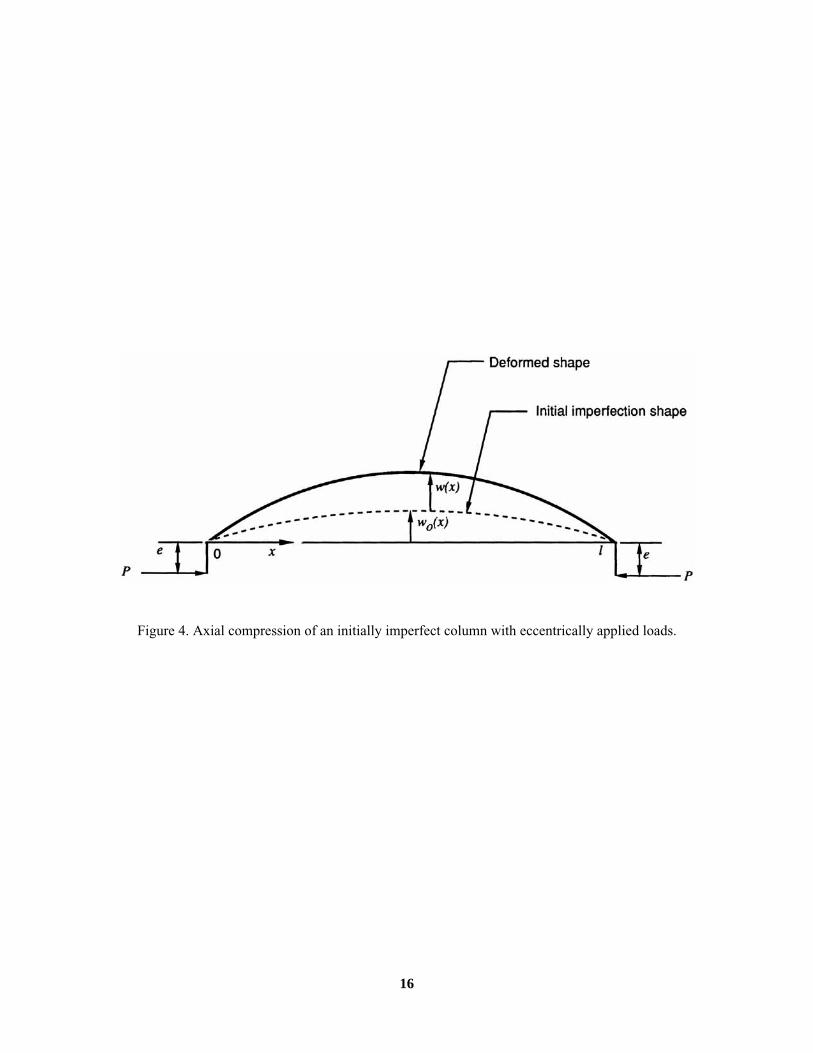
The deformed shape w(x) of a strut with an initial imperfection wo(x) and acted on by aCompressive axial load P applied at a distance e from the neutral axis is shown in figure 4.The linear differential equation and the appropriate boundary conditions to determine w(x) aregiven in equation (1) and are derived in ref. 8.

EId w

dxPw P(w e)

2

2 o+ = − + (1)

where

w w l( ) ( )0 0= =The solution to the homogeneous portion of equation (1) is

w B qxl

B qxlh =

+

1 2cos sinπ π (2)

3

where B1 and B2 are determined from the boundary conditions and q, the compressive axial loadnormalized by the Euler buckling load for the simply supported strut, is defined as

q =PP

=Pl

EIe

2

2π(3)

The initial imperfection wo(x) is assumed to be parabolic with a maximum magnitude of ε, andis given by

w =x x

o 42

εl l

−

(4)

Substituting equation (4) into equation (1), determining the particular solution, and applyingthe boundary conditions, results in the following expression for lateral displacement of acompressively loaded strut with a parabolic initial imperfection:

w(x)=2

2 2

2

8

2 21

82 2

2

2

επ

π π επ

π π

q

qx

l

qxl q

eq q x

− −

+ +

tan sin

+

−cosπ q x

e2

(5)

For small lateral displacements, total axial shortening can be calculated by superimposing thecontribution due to uniform axial compression on that due to lateral displacement. The axialshortening between any two arbitrary points x0 and x1 is found by integrating the axial strainbetween these limits. In order to represent both the effect of uniform axial compression and theeffect of lateral displacement, it is necessary to include both the linear term and the first nonlinearterm of axial strain. The equation for axial shortening is thus

δ =12

12

12

2

0

1

0

12

0

1dudx

dwdx

dxdudx

dxdwdx

dxx

x

x

x

x

x

+

= +

∫ ∫ ∫ (6)

To determine the axial shortening of a strut with an initial lateral imperfection wo(x) equation(6) must be modified. In this case the total lateral displacement after application of load is w(x) +wo(x) (see fig. 4). Therefore, the axial shortening due to the elastic deflection w(x) is

δ =dudx

dxd w w

dxdx

dwdx

dxx

xo

x

xo

x

x

+ +

−

∫ ∫ ∫

0

12

0

12

0

112

12

( ) (7)

The linear strain in the first term of equation (7) is the uniform axial compressive stressdivided by the Young s modulus of the strut. Making this substitution and evaluating the firstintegral gives

δ =Pl*EA

+ +

−

∫ ∫1

212

2

0

12

0

1d w wdx

dxdwdx

dxo

x

xo

x

x( ) (8)

where l* = x1 — x0.The remaining two terms in equation (8) can now be evaluated by substitution of the parabolic

initial imperfection wo given in equation (4) and the corresponding lateral displacement w givenin equation (5). The following integral expression is obtained:

δ = 32ε2

π 2ql2 + 8εe

l2 +

π 2qe2

2l2 tan2

π q2

cos2 π qx

2

xo

xl

- 2 tan π q

2 cos

π qx2

sin π qx

2 + sin2

π qx2

- 8ε2

4 l2 - 4xl + 4x 2 dx + Pl*

EA(9)

4

The total axial shortening of the strut can be determined by setting x0 = 0 and x0 = l in equation(9). Integration and simplification of this equation lead to the following expression:

δ = ε2 32 π q - sin (π q)

l (π q)3 1 + cos (π q) - 8

3l + εe

8 π q - sin (π q)l π q 1 + cos (π q)

+ e2 π q π q - sin (π q)

2l 1 + cos (π q) + Pl

EA (10)

Equation (10) is the sum of four terms that make specific contributions to the axial shorteningof the strut. The first term is due solely to the initial imperfection. The second term accounts forthe interaction between initial imperfection and load eccentricity. The third term is due solely tothe load eccentricity. Finally, the fourth term is the contribution due to uniform axialcompression.

It is common in linear imperfect strut analysis to assume a half-sine rather than a parabolicinitial imperfection shape because the homogeneous solution to the differential equation isalready of this form (se eq. (2)). Although the study is based on a parabolic initial imperfection, aderivation of the equation for axial shortening of a strut with a half-sine initial imperfection ispresented in appendix A.

Of concern in the analysis of axial shortening of eccentrically loaded columns with initialimperfections is the occurrence of large deflections and the importance of geometric nonlineari-ties. The nonlinear solution for end shortening of an eccentrically loaded column with a circularinitial imperfection is presented in reference 9. This solution is inherently transcendental andrequires the use of numerical iteration routines. Consequently, it is desirable to use the linearsolution presented in equation (10) for problems involving sufficiently small deflections. Acomparison of results from equation (10) with results from the nonlinear solution are presented inappendix B. From this comparison, loads are defined where the linear solution departs from thenonlinear solution by a specified percentage for ranges of the initial imperfection and loadeccentricity magnitudes.

Testing of Imperfect Slender Truss Struts

Eleven struts, sized for application to the Space Station Freedom truss, were tested todetermine their load-shortening behavior. Nine of the specimens were 5 m long and two of thespecimens were 7.1 m long. Before loading, each specimen was measured to determine its initialimperfection and cross-sectional uniformity. Descriptions of the test setup and imperfectionmeasurements of the specimens are presented in this section. Finally, experimental load-shortening data are presented for each specimen and compared with analytical predictions basedon the linear analysis developed in the preceding section.

Description of Test Setup

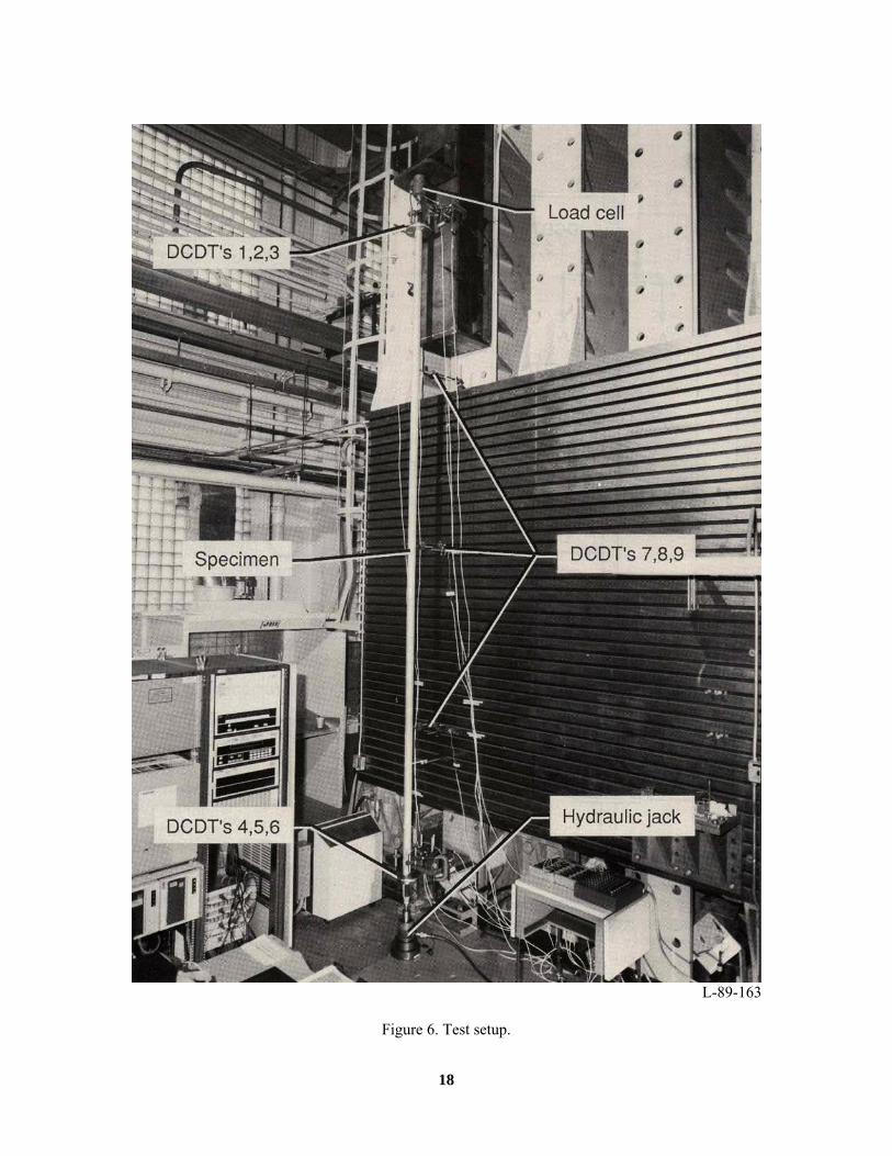
Before testing, each specimen was mated to quick-attachment erectable joint hardware of thetype shown in figure 3, and the assembly was accurately set to length. The specimen wasmounted vertically between a hydraulic jack for load introduction and a load cell for loadmeasurement. This test setup is diagramed in figure 5 and shown in figure 6.

Centerline shortening of each specimen was determined from direct current differentialtransformer (DCDT) measurements made at two stations along the length of the specimen(x0 and x1 inches from the bottom of the specimen). These locations spanned the portionof the strut with a uniform cross-sectional area, thus displacement measurements between themexcluded any deformation in the erectable end-joints. Displacement at the center of thespecimen cross section was calculated by averaging the readings of three DCDT s located at the

5

apexes of an equilateral triangle centered on the cross section. This process eliminatesthe effects of local bending rotations in the specimen regardless of the direction of rotation.The approximate location of the measurement stations and a section view of the upper stationshowing the DCDT placement are shown in figure 5. The axial shortening of the specimenbetween these two stations is determined by subtracting the centerline displacement at theupper station (DCDT s 1, 2, and 3) from the centerline displacement at the lower station(DCDT s 4, 5, and 6).

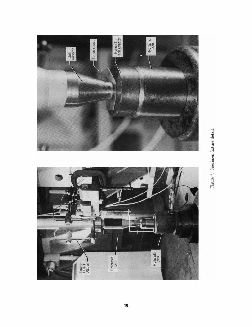
Details of the fixture used to provide a pinned-end restraint to the specimen are shown infigure 7. The left-hand photograph shows the lower end of the specimen, the lower DCDTstation, and the hydraulic jack. The right-hand photograph shows a close-up view of thespecimen end fixture. A special joint adaptor was attached to the node fitting portion of theerectable joint to cause end rotation of the specimen to occur at the theoretical node center(see fig. 3). Because of the arbitrary orientation of initial imperfections and eccentricities,it was impossible to identify, a priori, the preferred direction of buckling of the specimens.Therefore, it was necessary to provide an omnidirectional pinned-end restraint by incorporatinga hemispherical end on the joint adaptor and a mating hemispherical socket in the hydraulicjack adaptor. A thin sheet of greased Teflon was inserted between these adaptors to ensurea low-friction interface. Identical fixtures were used on both the top and the bottom of thespecimen.

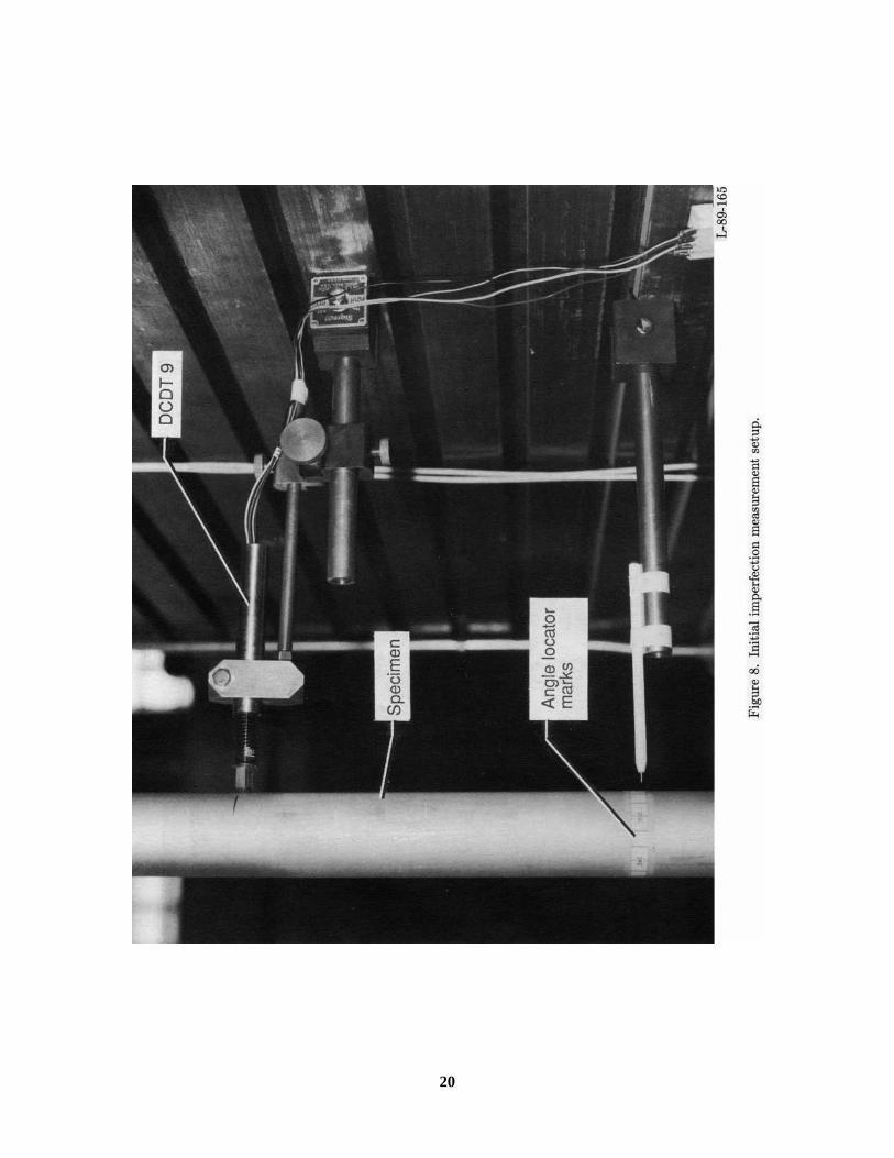
The initial imperfections of the specimens were determined from lateral DCDT measurementsmade along the strut length. Measurements were made at evenly spaced stations as the specimenwas rotated 360ß around its longitudinal axis. The lower lateral DCDT (DCDT 9) and a series ofindicator marks to locate the orientation angle around the circumference of the specimen areshown in figure 8. An explanation of the procedure used to determine initial imperfectionmagnitudes from these readings is presented in the following section.

Description of Specimens

Each specimen was measured to determine an initial imperfection magnitude and variations inits cross-sectional dimensions. Results of these measurements are presented below.

Specimen initial imperfection magnitudes. The initial imperfection was measured at threepoints along the length of the specimen: 0.25l, 0.50l, and 0.75l. To determine the imperfectionvalues at each point, DCDT readings were taken at 20ß increments as the strut was rotatedabout its longitudinal axis. The minimum reading was then subtracted from the maximumreading with the result divided by two to give the imperfection value at this point. These valuesfor the imperfection at the three span locations were used to obtain a least-squares regression fitof equation (4). The resulting expression for the best-fit ε is given in equation (11):

ε =2

173 4 31 4 1 2 3 4w w w/ / /+ +( ) (11)

where w 1/4, w1/2, w3/4 are the measured values of imperfection at 0.25l, 0.50l, and 0.75l,respectively.

To determine the quality of the parabolic curve fit of the imperfection data, the percent-rmsdifference (∆εrms) between the data and the best-fit parabolic curve is also calculated. Theseresults are presented in table I along with the specimen lengths and the location of the upper andlower stations for measuring axial displacement (see fig. 5). The parabolic curve fitapproximations to the actual imperfection shape of the specimens were found to exhibit rmserrors between 1.8 and 26 percent.

6

Table I. Specimen Lengths and Initial Imperfections

Specimen l, in. x0, in. x1, in. l*, in. ε, in. ∆εrms, %

1 196.8 8.1 188.7 180.6 0.071 26.02 196.8 8.1 188.7 180.6 .307 8.83 196.8 8.1 188.7 180.6 .187 16.64 196.8 8.1 188.7 180.6 .232 8.05 196.8 8.1 188.7 180.6 .215 10.86 196.8 8.1 188.7 180.6 .145 10.77 196.8 8.1 188.7 180.6 .265 10.08 196.8 8.1 188.7 180.6 .214 1.8

a9 196.8 8.5 186.9 178.4 .075 15.010 278.4 8.1 270.3 262.2 .681 3.211 278.4 8.1 270.3 262.2 .382 9.6

aThe values of x0 and x1 for specimen 9 are different from those for the other 5-m strutsbecause of a manufacturing error that necessitated the addition of a tubular aluminumextension to one end of the specimen.

Specimen cross-sectional variations. Ideally, the inner and outer layers of aluminum in thestrut cross section (see fig. 2) should be concentric and of constant thickness as should the layerof graphite/epoxy. The nominal design values for the thicknesses of each aluminum layer, thethickness of the graphite/epoxy layer, and the outer radius are 0.006, 0.060, and 1.066 in..,respectively.

The specimen cross sections showed a lack of concentricity between the inner and outer layersof aluminum and thus, significant variations from the nominal dimensions. This lack ofconcentricity results in a shift of the centroid of the cross section, and thus, a reduction in themoment of inertia and the introduction of a load eccentricity. In general, it was observed that thecross-sectional imperfections were aligned with the initial imperfection bow in the strut such thatall effects (load eccentricity, reduced cross-sectional moment of inertia, and initial strut bow)were additive in degrading the load-shortening performance of the strut.

Measurements of outside diameter and wall thickness were made at various orientationsaround both ends of each specimen and these values were used to derive average cross-sectionalproperties. For the purpose of these calculations, the three-layer, two-material, annular crosssection was assumed to be a single-layer, one-material annular cross section with an effectiveYoung s modulus to be determined from experiment.

A strut cross section in which the inner and outer circular surfaces are not concentric isshown in figure 9. The axes shown are centroidal and the distances to the centers of the innerand outer circular surfaces from the origin are defined as yi and yo, respectively. The radii ofthese inner and outer surfaces are ri and ro, respectively, and the minimum and maximumthicknesses are tmin and tmax, respectively. The difference in the minimum and maximumthicknesses is given by

∆t t t y yi o= max min ( )− = −2 (12)

The average thickness, t, is defined to be

t t t=12

( )max min+ (13)

From the definition of the centroid of a planar region, it follows that

ydA y r y rArea

o o i i∫ ⇒ == 0 2 2 (14)

7

During manufacture, the inside of the ends of each tube was machined on a lathe to accept atapered, bonded adaptor fitting for the erectable joint hardware. The center of machining was thecenter of the outside surface of the strut cross section. Therefore, after assembly, the center of thehemispherical end of the joint adaptor fitting (see fig. 7) was coincident with the center of theoutside surface. Accordingly, the center of the outside surface was assumed to be the point ofapplication of the load, and therefore the load eccentricity e is given by the following equation(see fig. 9):

e yo= (15)

Substituting equations (12) through (14) into equation (15) and simplifying gives thefollowing expression for load eccentricity in terms of the outer radius, the average thickness, andthe difference between the maximum and minimum thicknesses:

et r r t t

r t t

o o

o

=∆ 2 2

2

2

2 2

− +( )−( )

(16)

To quantify the concentricity effect, the eccentricity given by equation (16) can be expressedas a function of the concentricity error (yi — yo). Inserting equation (12) into equation (16) andsubstituting the nominal value of ro/t ¯ 14.8 gives

ey y r t r t

r ty y

i o o o

oi o=

( )

( ). ( )

− − +( )−

≈ −2 2 2 1

2 16 6 (17)

Thus the resulting load eccentricity is over six times greater than the concentricity error. Thisillustrates the importance of maintaining concentricity (or equal material distribution around thestrut circumference) during manufacture of the struts.

The minimum moment of inertia I for the eccentric cross section can be calculated byperforming the appropriate area integral. The result is

I y dA r r y r y rArea

o i i i o o= −( ) − −( )∫ 2 4 4 2 2 2 2

4=

π π (18)

The first term in this expression is the moment of inertia of the concentric cross section, and thesecond term is the reduction due to deviation from concentricity.

Substituting equations (12) through (16) into equation (18) and simplifying gives the equationfor cross-sectional moment of inertia in terms of the outside radius, the average thickness, and theapplied load eccentricity. This equation is

I r r t e rr

r tI e r

r

r to o o

o

op o

o

o

=π π π4

1 14 4 2 22

22 2

2

2− −[ ] −

−−

= −−

−

( )( ) ( )

(19)

where Ip is the moment of inertia of the perfect cross section (one with no concentricity error).A concentricity error does not affect the area of the cross section, which is given by

A r r r r to i o o= π π2 2 2 2−( ) = − −[ ]( ) (20)

Values for t, ∆t, and ro were determined from averaged measurements made at each end ofeach specimen and values for e, I, Ip, and A were calculated for each specimen using equation(17), equation (11), and equation (12). A summary of these measured and calculated values aswell as a list of the nominal design values for comparison are presented in table II.

8

Table II. Average Cross-Sectional Parameters for Test Specimens

Specimen r0, in. t, in. ∆t, in. e, in. Ι, in4 Ιp, in4 Α, in2

Nominal 1.066 0.072 0.000 0.000 0.248 0.248 0.4661 1.070 .089 .021 .056 .300 .302 .5752 1.072 .088 .014 .037 .299 .301 .5683 1.070 .086 .016 .044 .291 .293 .5554 1.069 .085 .015 .042 .288 .289 .5485 1.066 .091 .015 .038 .303 .304 .5846 1.064 .087 .026 .070 .287 .291 .5587 1.062 .074 .017 .055 .249 .251 .4778 1.069 .092 .027 .068 .306 .310 .591

a9 1.065 .093 .027 .067 .306 .309 .59510 1.065 .084 .015 .042 .281 .283 .54011 1.062 .084 .012 .034 .280 .281 .541

aBecause of problems in the manufacture of specimen 9, it was possible to make thesemeasurements at only one end; therefore, the values given do not represent a strut average.

On the average, these specimens were approximately 20 percent thicker than the nominaldesign, with as much as a 30-percent variation in thickness around any given cross section.However, the presence of errors in concentricity caused only 1-2 percent reductions in themoment of inertia. In the following section, results are presented from axial compression testsand analysis which illustrate the effect of these dimensional irregularities on the load-shorteningbehavior of the struts.

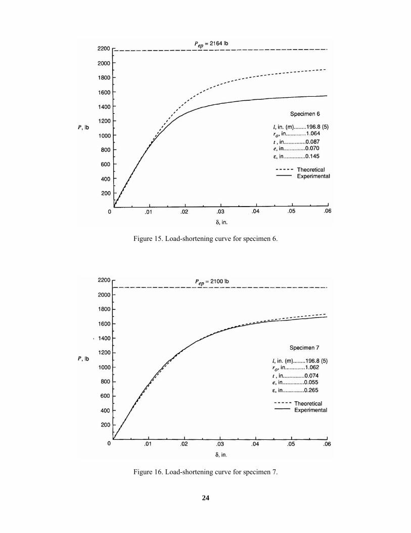
Results from axial compression analyses and tests. A value for the effective Young smodulus, E , for each specimen was determined by considering the initial slope of theexperimental load-shortening curve of the specimen. With this value and the values for thedimensional parameters given in tables I and II, the specimen s theoretical load-shortening curvecan be generated by solution of equation (9) or equation (10) for a series of load values. Equation(10) gives the axial shortening between the ends of the strut, and therefore cannot be used forcomparison with the experimental data. Consequently, theoretical load-shortening curves weregenerated by numerical integration of equation (9).

The experimental load-shortening curve for each specimen was determined using thecompression test setup previously described. During each test, the specimen was subjected to aslowly increasing compressive load while a real-time plot of the load-shortening curve becamenearly zero. Data from these tests are plotted in figures 10 through 20 for specimens 1 through11, respectively.

The initial slopes of these curves, EA/l*, were used to determine experimental values for E.These values are presented in table III for each specimen along with calculated values for theEuler buckling load (Pe = π2EI/l2); the perfect cross section Euler buckling load (Pep = π2EIp/l

2);and the normalized maximum loads achieved in each test, qmax. A comparison of Pe and Pep intable III illustrates the small reduction in I (and consequently Pep) resulting from lack ofconcentricity. Differences in the cross-sectional dimensions and effective Young s modulus ofdifferent specimens led to 10 percent variations in Euler buckling loads and effective axialstiffnesses.

9

Table III. Results From Axial Compression Tests

Specimen E, psi Pe, lb Pep, lb qmax ql

1 27.3 x 106 2088 2102 0.90 0.962 27.6 2108 2122 .80 .933 28.9 2141 2156 .86 .954 28.8 2106 2113 .83 .945 25.7 1979 1986 .89 .946 29.2 2134 2164 .72 .957 32.9 2083 2100 .83 .938 27.8 2166 2194 .87 .949 26.7 2080 2100 .91 .96

10 27.7 1011 1018 .77 .9011 27.7 1014 1018 .84 .94

Also included in table III are load values ql at which the linear load-shortening analysis differsfrom the nonlinear analysis by 2 percent. These values were determined from analyses presentedin appendix B. None of the specimens were tested to a load level above these limiting values(qmax < ql). Thus, geometric nonlinearities were unimportant, and the linear load-shorteninganalysis presented in equation (9) and equation (10) is applicable.

The theoretical load-shortening curves as determined from numerical integration of equation(9) are shown in figures 10 through 20. Good agreement is seen between the theoretical andexperimental curves for all of the specimens except 4, 6 and 9. The specimens that had thegreatest rms error in the parabolic approximation of their imperfections (specimens 1 and 3)showed reasonably good agreement between the theoretical and experimental load-shorteningcurves. Therefore, the poor agreement for specimens 4, 6, and 9 may be due to variations in theircross-sectional dimensions near the midspan. The cross-sectional dimensions in table II weredetermined from measurements made near the ends of the specimens (only one end for specimen9); thus, any significant cross-sectional variations near the middle of the strut would not berepresented in these measurements.

Initial imperfections and errors in cross-sectional concentricity significantly degraded the load-shortening behavior of all specimens as evidenced by the fact that all the specimens deviatedmarkedly from linear elastic behavior characteristic of a corresponding perfect strut. This impliesthat control of cross-sectional concentricity and strut straightness is very important to achievesatisfactory performance from long slender truss struts.

Concluding Remarks

The results of a study of the load-shortening behavior of initially imperfect struts under theaction of eccentrically applied compressive loads have been presented. Linear analysis has beenperformed and compared with experimental results from 11 developmental aluminum-cladgraphite/epoxy truss struts. These comparisons showed good agreement for most specimens.

The specimens were measured to determine deviations from straightness and nominal cross-sectional dimensions. These measurements were used to calculate values for initial imperfectionmagnitude and load eccentricity, as well as cross-sectional area and moment of inertia. It wasdetermined that the load eccentricity resulting from an error in cross-sectional concentricity isover six times greater than the concentricity error.

Deviations from concentricity coupled with initial imperfections in straightness led tosignificantly degraded load-shortening behavior for all specimens tested. This illustrates theimportance of maintaining concentricity and straightness during the manufacture of the struts.

10

Appendix A

Axial Shortening of an Eccentrically Loaded Strut With a Half-Sine InitialImperfection

The half-sine initial imperfection given in equation (A1) is commonly selected for linearimperfect strut analysis because it is the same shape as the homogeneous solution to thegoverning differential equation (see eq. (1)). The solution for axial shortening of an eccentricallyloaded strut with this initial imperfection follows the same steps as outlined for the parabolicinitial imperfection.

w =o ε πsin

xl

(A1)

Substituting equation (A1) into equation (1), determining the particular solution, and applyingthe boundary conditions results in the following expression for lateral displacement of aneccentrically loaded strut with a half-sine initial imperfection:

w(x)=qε π

π

ππ

1 2 2−

+ −

−

qxl

e

q

qq

xl

esincos( / )

cos (A2)

Equation (8) is evaluated by substitution of the half-sine initial imperfection wo given inequation (A1) and the corresponding lateral displacement w given in equation (A2). Thefollowing integral expression is obtained for the axial shortening between any two points x0 andx1 of the strut:

δ επ π επ

π

π π π=

12

1

11

2

1 2 2

2

22

2

20

1

l q

xl

e q

q l q

q q x

lxlx

x

−

−

+−

−

∫ ( )

cos( ) cos( / )

sin cos

+

−

+e q

l q

q q x

ldx

PlEA

π

π

π π

cos( / )sin

*

2 2

2

2 (A3)

The total axial shortening of the strut can be determined by setting x0 = 0 and x0 = l (thus l* =l) in equation (A3). The result is

δ ε π π ε π π π π

π=

22

2

2

22

4 1 42

1 2 1l q le

q

l qe

q q q

l q

PlEA( ) ( )

sin( )

cos( )−−

+−

+−[ ]

+[ ]

+ (A4)

Recall that e is the load eccentricity, ε is the midlength magnitude of the half-sineimperfection, and q is the applied compressive load normalized to the Euler buckling load.Equation (A4) is the sum of four terms similar to those in equation (10). In fact, the third andfourth terms are identical to those in equation (10) because they account for the effects of loadeccentricity and uniform axial compression, which are unchanged from the first case. Thedifferent assumptions for initial imperfection shape account for the differences in the first twoterms of equation (10) and equation (A4).

11

Appendix B

Importance of Geometric Nonlinearities

A recent study (ref. 9) has used the nonlinear formulation for axial compression of a strut (ref.8) to investigate the load-shortening behavior of an eccentrically loaded strut with a constant-curvature (i.e., circular) initial imperfection. For small initial imperfection magnitudes, theparabolic shape presented in equation (4) closely approximates the circular shape assumed in thenonlinear analysis of reference 9. Thus, comparison of the linear solution presented in equation(10) with the corresponding nonlinear solution from reference 9 will identify the importance ofgeometric nonlinearities.

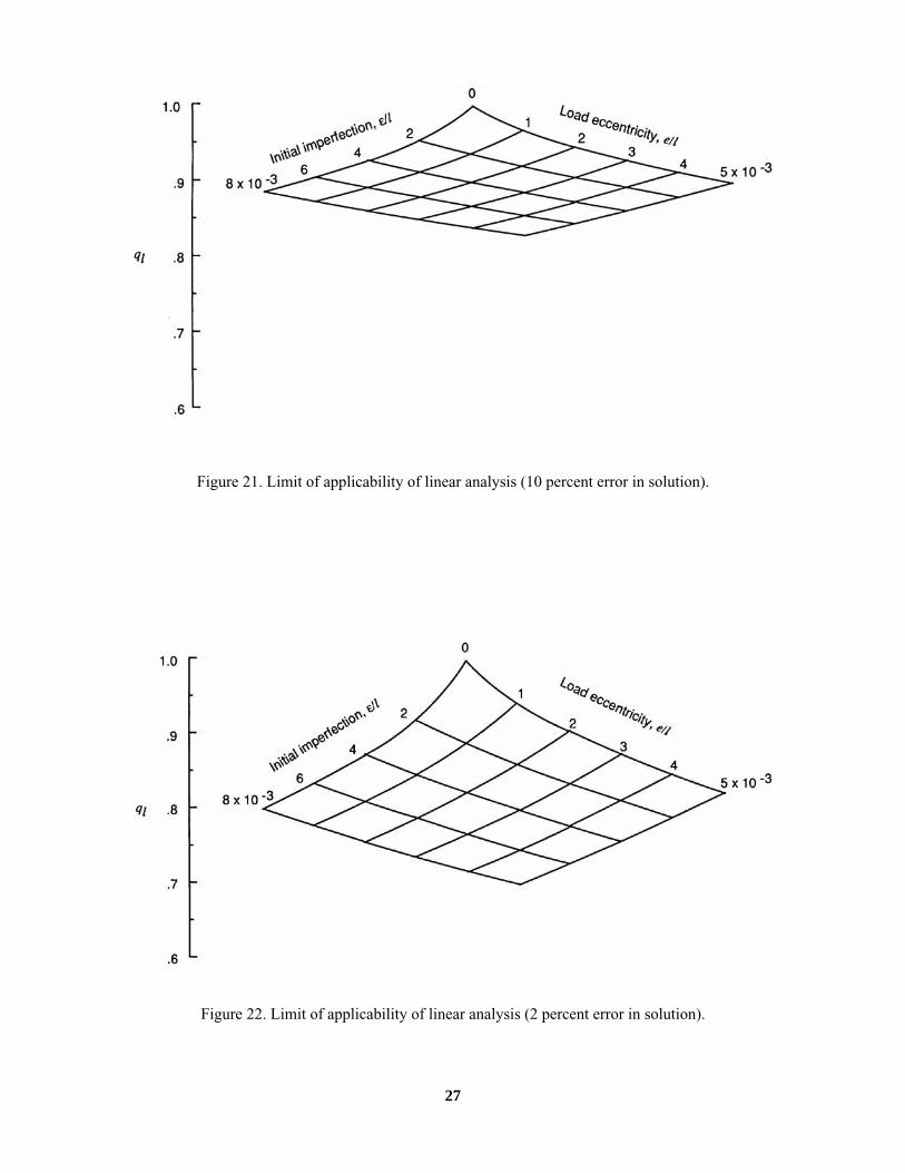
Linear analysis predicts larger deformations for large loads than those predicted with nonlinearanalysis. From equation (10), it is evident that as q approaches 1, linear analysis predicts infiniteaxial shortening. However, nonlinear analysis predicts finite axial shortening for q = 1. The errorin linear analysis increases with increasing load. Therefore, a load ql at which the axialshortening from linear analysis is in error by a specified amount is defined as the limit ofapplicability of linear analysis.

Values for ql can be determined for ranges of the strut parameters e/l and ε/l and general plotsof this limiting load can be constructed. Figure 21 presents a carpet plot of ql for an allowableerror in linear analysis equal to 10 percent, and figure 22 presents a similar plot for an allowableerror equal to 2 percent. These plots can be used to readily determine the limit of applicability oflinear analysis for specimens with given values of e/l and ε/l. All experimental load-shorteningdata analyzed in the present study fall below the 2-percent-error limit for the respective specimen.Therefore, errors in linear analysis due to geometric nonlinearities are less than 2 percent.

12

References

1. Mikulas, Martin M., Jr.; Croomes, Scott D.; Schneider, William; Bush, Harold G.; Nagy, Kornell; Pelischek,Timothy; Lake, Mark S.; and Wesselski, Clarence: Space Station Truss Structures and ConstructionConsiderations. NASA TM-86338, 1985.

2. Mikulas, Martin M., Jr.; and Bush, Harold G.: Design, Construction and Utilization of a Space Station AssembledFrom 5-Meter Erectable Struts. NASA TM-89043, 1986.

3 . Johnson, R. R.; Bluck, R. M.; Holmes, A. M. C.; and Kural, M. H.: Development of Space Station StrutDesign. Materials Sciences for the Future - 31st International SAMPE Symposium and Exhibition, JeromeL. Bauer and Robert Dunaetz, eds., Soc. for the Advancement of Meterial and Process Engineering, 1986,pp. 90-102.

4. Ring, L. R.: Process Development and Fabrication of Space Station Type Aluminum-Clad Graphite EpoxyStruts. NASA CR-181873, 1990.

5. Heard, Walter L., Jr.; Bush, Harold G.; Watson, Judith J.; Spring, Sherwood C.; and Ross, Jerry L.:Astronaut/EVA Construction of Space Station. A Collection of Technical Papers — AIAA SDM Issues ofthe International Space Station, Apr. 1988, pp. 39-46 (Available as AIAA-88-2459.)

6. Heard, W. L., Jr.; Bush, H. G.; and Agranoff, Nancy: Buckling Tests of Structural Elements Applicable to LargeErectable Space Trusses. NASA TM-78628, 1978.

7. Razzaq, Zia; Voland, R. T.; Bush, H. G.; and Mikulas, M. M., Jr.: Stability, Vibration, and PassiveDamping of Partially Restrained Imperfect Columns. NASA TM-85697, 1983.

8. Timoshenko, Stephen P.; and Gere, James M.: Theory of Elastic Stability, Second ed. McGraw-Hill Book Co.,1961.

9. Fichter, W. B.; and Pinson, Mark W.: Load-Shortening Behavior of an Initially Curved EccentricallyLoaded Column. NASA TM-101643, 1989.

13

14

15

16

Figure 4. Axial compression of an initially imperfect column with eccentrically applied loads.

17

Figure 5. Diagram of test setup.

18

L-89-163

Figure 6. Test setup.

19

20

21

Figure 9. Nonconcentric strut cross section.

Figure 10. Load-shortening curve for specimen 1.

22

Figure 11. Load-shortening curve for specimen 2.

Figure 12. Load-shortening curve for specimen 3.

23

Figure 13. Load-shortening curve for specimen 4.

Figure 14. Load-shortening curve for specimen 5.

24

Figure 15. Load-shortening curve for specimen 6.

Figure 16. Load-shortening curve for specimen 7.

25

Figure 17. Load-shortening curve for specimen 8.

Figure 18. Load-shortening curve for specimen 9.

26

Figure 19. Load-shortening curve for specimen 10.

Figure 20. Load-shortening curve for specimen 11.

1100

1000

900

800

700

600

500

400

300

200

100

1100

1000

900

800

700

600

500

400

300

200

100

27

Figure 21. Limit of applicability of linear analysis (10 percent error in solution).

Figure 22. Limit of applicability of linear analysis (2 percent error in solution).

National Aeronautics andSpace Administration

Report Documentation Page

1. Report No.

NASA TM-41742. Government Accession No. 3. Recipient’s Catalog No.

4. Title and Subtitle

Analysis and Testing of Axial Compression in Imperfect Slender5. Report Date

February 1990Truss Struts 6. Performing Organization Code

7. Author(s)

Mark S. Lake and Nicholas Georgiadis8. Performing Organization Report No.

L-167129. Performing Organization Name and Address

NASA Langley Research Center10. Work Unit No.

506-43-41-02Hampton, VA 23665-5225 11. Contract or Grant No.

12. Sponsoring Agency Name and Address

National Aeronautics and Space Administration13. Type of Report and Period Covered

Technical MemorandumWashington, DC 20546-0001 14. Sponsoring Agency Code

15. Supplementary Notes

16. Abstract

This study addresses the axial compression of imperfect slender struts for large space structures.The load-shortening behavior of struts with initially imperfect shapes and eccentric compressiveend loading is analyzed using linear beam-column theory and results are compared with geometri-cally nonlinear solutions to determine the applicability of linear analysis. A set of developmentalaluminum-clad graphite/epoxy struts sized for application to the Space Station Freedom truss aremeasured to determine their initial imperfection magnitude, load eccentricity, and cross-sectionalarea and moment of inertia. Load-shortening curves are determined from axial compression testsof these specimens and are correlated with theoretical curves generated using linear analysis.

17. Key Words (Suggested by Author(s))

Column stabilityEccentricity loadInitial imperfectionSpace station

18. Distribution Statement

Unclassified-Unlimited

19. Security Classif. (of this report)

Unclassified20. Security Classif. (of this page)

Unclassified21. No. of Pages

2822. Price

A03NASA FORM 1626 OCT 86 NASA-Langley, 1990

For sale by the National Technical Information Service, Springfield, Virginia 22161-2171