Analysis, Control, andDesign Optimization ofEngineering Mechanics

Systems

Esubalewe Lakie Yedeg

PhD Thesis, May 2016

Department of Computing ScienceUmea UniversitySE-901 87 UmeaSweden

Department of Computing ScienceUmea UniversitySE-901 87 Umea, Sweden

yedegl@cs.umu.se

copyright c© 2016 Esubalewe Lakie Yedeg

UMINF: .. ..ISSN: ....-....ISBN: ...-..-....-...-.

Electronic version available at http://umu.diva-portal.org/Printed by Print & Media, Umea UniversityUmea, Sweden 2016

Abstract

This thesis considers applications of gradient-based optimization algorithms to thedesign and control of some mechanics systems. The material distribution approach totopology optimization is applied to two design different acoustic devices, a reactivemuffler and an acoustic horn, and optimization is used to control a ball pitching robot.

Reactive mufflers are widely used to attenuate the exhaust noise of internal combus-tion engines by reflecting the acoustic energy back to the source. A material distributionoptimization method is developed to design the layout of sound-hard material insidethe expansion chamber of a reactive muffler. The objective is to minimize the acousticenergy at the muffler outlet. The presence or absence of material is represented bydesign variables that are mapped to varying coefficients in the governing equation.An anisotropic design filter is used to control the minimum thickness of materialsseparately in different directions. Numerical results demonstrate that the approachcan produce mufflers with high transmission loss for a broad range of frequencies.

For acoustic devices, it is possible to improve their performance, without addingextended volumes of materials, by an appropriate placement of thin structures withsuitable material properties. We apply layout optimization of thin sound-hard materialin the interior of an acoustic horn to improve its far-field directivity properties.Absence or presence of thin sound-hard material is modeled by a surface transmissionimpedance, and the optimization determines the distribution of materials along a“ground structure” in the form of a grid inside the horn. Horns provided with theoptimized scatterers show a much improved angular coverage, compared to the initialconfiguration.

The surface impedance is handled by a new finite element method developed forHelmholtz equation in the situation where an interface is embedded in the compu-tational domain. A Nitsche-type method, different from the standard one, weaklyenforces the impedance conditions for transmission through the interface. As opposedto a standard finite-element discretization of the problem, our method seamlesslyhandles both vanishing and non-vanishing interface conditions. We show the stabilityof the method for a quite general class of surface impedance functions, provided thatpossible surface waves are sufficiently resolved by the mesh.

The thesis also presents a method for optimal control of a two-link ball pitchingrobot with the aim of throwing a ball as far as possible. The pitching robot is connectedto a motor via a non-linear torsional spring at the shoulder joint. Constraints on themotor torque, power, and angular velocity of the motor shaft are included in themodel. The control problem is solved by an interior point method to determine theoptimal motor torque profile and release position. Numerical experiments show theeffectiveness of the method and the effect of the constraints on the performance.

iii

Sammanfattning

Denna avhandling anvander sig av gradientbaserade optimeringsalgoritmer for designoch styrning av ett antal mekaniksystem. Topologioptimering med materialdistru-butionsmetoden anvands for att formge tva olika akustiska anordningar, en reaktivljuddampare och ett akustiskt horn. Dessutom anvands en optimeringsmetod for attstyra en bollkastande robot.

Reaktiva ljuddampare anvands ofta for att dampa avgasljudet hos forbranningsmo-torer genom att reflektera den akustiska energin tillbaka till kallan. En materialdistri-butionsmetod har utvecklats for att utforma fordelningen av ljudhart material inutiexpansionskammaren i en reaktiv ljuddampare. Malet ar att minimera den akustiskaenergin vid ljuddamparens utlopp. Narvaro eller franvaro av material representeras avdesignvariabler som avbildas till varierande koefficienter i ljudutbredningsmodellensekvation. Ett anisotropt designfilter anvands for att separat begransa den minimalatillatna materialtjockleken i olika riktningar. De numeriska resultaten visar att metodenkan generera ljuddampare med hoga transmissionsforluster for ett brett frekvensband.

For akustiska komponenter ar det ofta mojligt att paverka prestanda, utan attbehova anvanda omfattande volymer av material, genom en lamplig placering avtunna strukturer med lampliga materialegenskaper. Vi optimerar utbredningen av tuntljudhart material i det inre av ett akustiskt horn for att forbattra hornets spridningse-genskaper i fjarrfaltet. Franvaro eller narvaro av tunt ljudhart material modellerasgenom en varierande akustisk impedans over ett antal givna ytor, och en optime-ringsalgoritm bestammer fordelningen av material utmed en grundstruktur i form avett galler inuti hornet. Hornen som ar forsedda med de optimerade spridarna visaren mycket forbattrad vinkeltackning jamfort med den ursprungliga konfigurationen.Ytimpedanserna hanteras numeriskt med hjalp av en ny finita-elementmetod somutvecklats for Helmholtz ekvation i narvaro av impedansytor i berakningsdomanen.En metod av Nitschetyp, som skiljer sig fran standardversionen, anvands for en svagformulering av impedansenvillkoren. I motsats till standardmetoden for hantering avimpedansytor klarar var metod att somlost hantera fallen da transmissionsimpedansenar saval noll som nollskild. Vi visar att metoden ar stabil for en forhallandevis allmannklass av ytimpedansfunktioner, forutsatt att eventuella ytvagor ar tillrackligt upplosaav berakningsnatet.

Avhandlingen presenterar ocksa en metod for optimal styrning av en tvalanksbollkastande robot i syfte att kasta bollen en sa lang stracka som mojligt. Robotarmen aransluten till en motor via en olinjar torsionsfjader vid armens axelled. Begransningar formotorns vridmoment samt kraften och vinkelhastigheten hos motoraxeln ar inkluderadei modellen. Styrproblemet loses med hjalp av en inrepunktsmetod som bestammer denoptimala motormomentsprofilen samt frigoringslaget for bollen. Numeriska experimentpavisar metodens effektivitet och belyser de palagda bivillkorens effekt pa kastlangden.

v

Preface∗

This thesis consists of introductions to the subject of topology optimization andNitsche-type methods for interface problems and the following papers.

Paper I Esubalewe Lakie Yedeg, Eddie Wadbro, and Martin Berggren, Interiorlayout topology optimization of a reactive muffler. Structural and Multidis-ciplinary Optimization, vol. 53, pp. 645–656, 2016.

Paper II Esubalewe Lakie Yedeg, Eddie Wadbro, Peter Hansbo, Mats G. Larson, andMartin Berggren, A Nitsche-type Method for Helmholtz Equation with anEmbedded Acoustically Permeable Interface. Computer Methods in AppliedMechanics and Engineering, vol. 304, pp 479–500, 2016.

Paper III Esubalewe Lakie Yedeg, Eddie Wadbro, and Martin Berggren. Layoutoptimization of thin sound-hard material to improve the far-field directivityproperties of an acoustic horn. Submitted for publication, 2016.

Paper IV Esubalewe Lakie Yedeg. On the use of thin structures to control the far-fieldproperties of an acoustic devices. Technical Report UMINF 16.12, Dept.of Computing Science, Sweden, 2016.

Paper V Esubalewe Lakie Yedeg and Eddie Wadbro. State constrained optimalcontrol of a ball pitching robot. Mechanism and Machine Theory, vol. 69,pp. 337–349, 2013.

This work has been financially supported in part by the Swedish Foundation forStrategic Research, Grant No. AM13-0029, and by the Swedish Research Council,Grant No. 621-2013-3706.

∗The papers have been re-typeseted to fit the booklet’s style. There may be minor typographicaldifferences from the published papers.

vii

Acknowledgement

This thesis would not have been possible without the inspiration, encouragement, andsupport of several individuals. I take this opportunity to give special thanks to thefollowing people.

First and foremost, I would like to express my sincere gratitude to my scientificadvisor, Martin Berggren for giving me the chance to join his research group andfor his continuous guidance, inspiration, encouragement, and support. He has been athoughtful and wonderful advisor, and without him this thesis would not have beencompleted or written. Martin, thank you for invaluable discussions and incrediblefeedback in my work. I have learned quite a lot from you.

I would also like to extend my appreciation to my co-advisor Eddie Wadbro forinteresting and fruitful discussions. I am grateful for his boundless support, especiallywhen I desire an advice on Matlab implementation. He was always open to me wheneverI needed his advice on research or other issues.

My deep gratitude also goes to all colleagues at UMIT research lab and the De-partment of Computing Science for the friendly and pleasant working atmosphere. Inparticular, I am grateful to members of the Design and Optimization research groupand system administrators.

I would like to extend my thanks to all Ethiopian friends who live in Umea, especiallyMeseret, Anteneh, Ewnetu, and their family who made me feel at home during mystay here. Meseret you are special for my family and I really thank you for everythingyou have done. I am thankful to Enideg and Fiseha for their support.

I would like to say a heartfelt thank you to my parents, Wubit Aragaw and LakieYedeg for always believing in me and for their unconditional support, encouragementand prayers. Without their support and prayers this work would not have been possible.Wubit, I always love you, you played a major role in shaping my life and you havebeen the rock of our family. I am also grateful to my brother Bekalu Lakie, my uncleAshagre Yedeg and their family for supporting me in whatever way they could. I wouldalso like to thank my parents-, brothers-, and sisters-in-law for their steady supportand prayers.

Last but not least, my deep and special appreciation goes to my wife, Tigist Muluken,who has given me the strength, support, encouragement and inspiration. Tigist, thankyou for your unconditional love and everything that comes to my life with you. I willnever forget your patience, sacrifices and suffering that you endured in taking care ourchildren, especially when I stay late in office. I also want to acknowledge my daughter,Yeabsira, and my son, Elias. I am so proud to be your father, you are sweet, positiveand cheerful kids. Finally, I would like to thank everybody who have contributed eitherdirectly or indirectly to this Thesis, as well as express my apology that I could notmention personally one by one.

Thank you!Esubalewe Lakie YedegUmea, May 2016

ix

I dedicate this thesis tomy mother, Wubit Aragaw, andmy beloved wife, Tigist Muluken.

I love you all dearly.

xi

Contents

1 Introduction 1

2 Topology Optimization by Material Distribution 32.1 Problem formulation . . . . . . . . . . . . . . . . . . . . . . . . . . . . 32.2 Discretization . . . . . . . . . . . . . . . . . . . . . . . . . . . . . . . . 42.3 Penalization . . . . . . . . . . . . . . . . . . . . . . . . . . . . . . . . . 52.4 Numerical instabilities and regularization . . . . . . . . . . . . . . . . 6

3 Summary of Paper I 93.1 Introduction . . . . . . . . . . . . . . . . . . . . . . . . . . . . . . . . . 93.2 Problem description . . . . . . . . . . . . . . . . . . . . . . . . . . . . 93.3 Selected numerical results . . . . . . . . . . . . . . . . . . . . . . . . . 11

4 Nitsche-Type Methods for Interface Problems 154.1 Problem formulation and preliminaries . . . . . . . . . . . . . . . . . . 154.2 A Finite Element Method . . . . . . . . . . . . . . . . . . . . . . . . . 174.3 Consistency and Coercivity . . . . . . . . . . . . . . . . . . . . . . . . 184.4 Convergence Analysis . . . . . . . . . . . . . . . . . . . . . . . . . . . 20

5 Summary of Paper II 235.1 Introduction . . . . . . . . . . . . . . . . . . . . . . . . . . . . . . . . . 235.2 Interface problems . . . . . . . . . . . . . . . . . . . . . . . . . . . . . 245.3 Selected numerical results . . . . . . . . . . . . . . . . . . . . . . . . . 26

6 Summary of Paper III and Paper IV 296.1 Introduction . . . . . . . . . . . . . . . . . . . . . . . . . . . . . . . . . 296.2 Problem description . . . . . . . . . . . . . . . . . . . . . . . . . . . . 306.3 Optimization problem . . . . . . . . . . . . . . . . . . . . . . . . . . . 326.4 Sensitivity Analysis . . . . . . . . . . . . . . . . . . . . . . . . . . . . . 336.5 Selected numerical results . . . . . . . . . . . . . . . . . . . . . . . . . 34

7 Summary of Paper V 357.1 Introduction . . . . . . . . . . . . . . . . . . . . . . . . . . . . . . . . . 35

xiii

7.2 Problem formulation . . . . . . . . . . . . . . . . . . . . . . . . . . . . 357.3 Selected numerical results . . . . . . . . . . . . . . . . . . . . . . . . . 38

xiv

Chapter 1

Introduction

Mechanical devices play an important role in our daily life. How to “optimally” designthem while satisfying the required system and design constraints is an importantengineering concern. We assume that the optimality of the design can be measured byan objective function that quantifies, for example, construction cost, strength of thedesigned structure, or some other performance measure. If a particular design makesthe objective function as high or low as possible, depending the objective, it is calledan optimal design.

Numerical design optimization of mechanical devices seeks to acquire, using acombination of simulation and numerical optimization algorithms, the best performanceof the device while satisfying some set of constraints. The subject is becoming moreimportant due to material resource limitations, the development of computationalalgorithms, and the availability of high-performance computers. During the last threedecades, the subject has developed rapidly with new theoretical insights, computationalmethods, and application areas. In general, numerical design optimization approachescan be classified into three main groups, namely sizing optimization, shape optimization,and topology optimization.

In sizing optimization, the conceptual geometry of the device is fixed during theoptimization process, and the goal is to find the optimal values of some free parametersof the structure, such as thickness, length, or radius of individual components. In shapeoptimization problems, the shape of the boundaries is subject to optimization, but theconceptual layout is predetermined. The design variables are typically some kind ofparameterization of the design boundaries. Topology optimization is the most generaland flexible approach to numerical design optimization, where for every point in thedesign region, it is to be determined whether the point is occupied by a material or not.Thus, the shape as well as the connectedness of the individual parts of the structureare not known a priori. Topology optimization can be seen as a generalization of sizingand shape optimization.

The behaviour of mechanical devices can often be modeled by partial differentialequations, such as the equations of elasticity, fluid mechanics, or acoustics. Thesemodels, ideally, represent the interaction of the device with its surroundings. Determin-

1

ing exact solutions of partial differential equations are possible only in some specialcases. In general, finding approximate solutions of partial differential equations relyon numerical techniques. The finite element method is one of the major techniques fornumerical solutions of partial differential equations.

Many mechanical systems can be modeled by ordinary differential equations. Thesesystems change with respect to time or any other independent variable according tothe equation. It is often possible to guide these systems from one state to anotherpredefined state by applying some kind of external force or control. It may also bepossible to carry out the same task in different ways. If there are more than one wayof performing the task, then it may be possible to choose the “best” way. The bestway can be quantified by using a measure of performance of the system; this measureis often called “cost function”, “objective function”, or “performance index”. Theexternal force applied to the system corresponding to the best performance is calledthe optimal control.

Optimal control also denotes the process of determining control and state trajectoriesfor a system over a given period of time to minimize or maximize an objective function.Optimal control is related to the theory of calculus of variations. The theory of optimalcontrol has been widely studied and is used in many areas since the beginning of theso-called “modern” control theory in the 1960s [1].

In general, control systems are classified into two broad categories: closed loop andopen loop systems. In closed-loop systems, also called feedback control systems, theinput is affected by the systems output directly or indirectly. It uses the input andsome portion of the output to maintain a prescribed relationship between the outputand the reference input. However, in open-loop control systems, sometimes calledoff-line or non-feedback control systems, the system output does not affect the controlinput in any form. In this case, the system is free from any change in response to theoutput of the process. Standard control theory mostly concerns closed-loop systems,and these are the ones used in most engineering control applications. In contrast, theopen-loop systems are useful in more special situations. In this thesis, we consider thedesign of such open-loop systems.

In this thesis, we use the optimal control and topology optimization ideas in twodifferent areas. First the topology optimization method is used to determine theinternal layout of a reactive muffler to minimize the acoustic energy at the outlet.The method is also used to improve the far-field properties of an acoustic horn bydistributing thin sound-hard material in the interior of the horn. We use the conceptof acoustic transmission impedance to model the acoustic properties of thin material.A new finite element method for Helmholtz equation with embedded interface isformulated to numerically handle the transmission impedance. The Method of MovingAsymptotes [2] is used to solve the optimization problems. Finally, we apply theoptimal control approach to determine the control of a ball pitching robot in order tothrow a ball as far as possible. The open-loop control problem is solved numericallyusing Matlab’s fmincon.

2

Chapter 2

Topology Optimization by Material

Distribution

Topology optimization is a mathematical approach to optimize the material layoutof a device within a given design space such that a certain performance criterion ismaximized or minimized, depending the objective, for a given set of conditions. Startingfrom the publication of the pioneering paper by Bendsøe and Kikuchi [3], topologyoptimization methods for continuum structures have been expanded significantly andapplied to many practical engineering problems. Topology optimization has beenused starting from designing materials at micro-level, see for example the works ofSigmund [4], Zhou & Li [5], and Jensen et al. [6], to large-scale designs such as bridgesand buildings, and for components within the automobile and aircraft industries, seefor example the works of example Borrvall & Petersson [7], Guan et al. [8], Wang etal. [9], and Krog et al. [10].

The field of topology optimization is dominated by methods that apply the materialdistribution concept, that is, when the design variables somehow represent local materialproperties. Most numerical methods for topology optimization rely on finite elementmethods for performance evaluations. In this case, the design domain is discretizedinto a fine mesh of elements, and the purpose of the algorithm is to find the optimalmaterial distribution by determining for each element in the design domain whetherit should be filled with material (solid element) or not (element with air). In thenext sections, a brief overview on topology optimization by the material distributionmethod is given.

2.1 Problem formulation

In general, a topology optimization problem consists of an objective function, a designdomain, design constraints, and a state equation. Let Ω be the design domain andΩm ⊂ Ω the region in the design domain occupied by solid material. The distributionof material in Ω is usually modeled by a material indicator function α, defined as

3

α(x) = 1, if x ∈ Ωm and α(x) = 0 otherwise. Mathematically, a topology optimizationproblem in its general form is given by

minα∈U

J(α, u) (2.1a)

s.t. a(α;u, v) = `(v) ∀v ∈ V, (2.1b)

C(α, u) ≤ 0, (2.1c)

where U = α : α(x) ∈ 0, 1, x ∈ Ω is the set of admissible designs, J is an objectivefunction to measure the performance, u denotes the state variable that solves thestate equation, C is a constraint function, and V is an appropriate function space. Thedesign and the state variables are related by the state equation, in this case given bythe variational form (2.1b).

Remark : In acoustics related topology optimization problems, the material indicatorfunction α is 1 in the region of air and 0 in the region that is occupied by sound-hardmaterial.

The prototype problem of this kind is the classical problem of minimizing thecompliance, J = `(u) (equivalent to maximizing the stiffness), of a mechanical structuresubject to state equation (2.1b), the governing equation of linear elasticity, and thevolume constraint, C(α) =

∫Ωα(x)dx − V ≤ 0. Here, V is the upper bound of the

volume occupied by solid material. To guarantee coercivity of the bilinear form, thematerial indicator function should not be zero. Therefore, the space of admissibledesigns U = α : α(x) ∈ 0, 1, x ∈ Ω is usually replaced by U = α : α(x) ∈ε, 1, x ∈ Ω for a small constant ε > 0, such that α(x) = ε for x ∈ Ω− Ωm.

In many cases, topology optimization problems of the form (2.1) are ill-posed.Typically, the ill-posedness is due to the existence of minimizing sequences that do notconverge [11], which, after discretization, usually, manifests itself as mesh dependencyin the numerical solution. A relaxation method can be used to address this problem.It also allows the use of gradient-based optimization algorithms. By letting α takevalues in the continuous range [ε, 1], the binary optimization problem (2.1) becomes

minα∈U

J(α, u), (2.2a)

s.t. a(α;u, v) = `(v) ∀v ∈ V, (2.2b)

C(α, u) ≤ 0, (2.2c)

where U = α : ε ≤ α(x) ≤ 1, x ∈ Ω.In the case of compliance minimization, there exist a unique solution of problem (2.2).

The proof of the existence of a solution can be found in Section 5.2 of the book [12]by Bendsøe and Sigmund.

2.2 Discretization

Numerical methods are typically used to obtain an approximate solution of optimizationproblem (2.2). Following a finite element procedure, the domain Ω is partitioned into

4

N small subdomains called elements Ek, k = 1, . . . , N , such that Ω = ∪Nk=1Ek. Thematerial indicator function α is approximated by an element-wise constant functionαh. The state variable u is approximated by uh ∈ Vh(Ω), where Vh ⊂ V is a space ofcontinuous and element-wise polynomial functions. The discrete state variable uh isthe solution of the discrete state equation for a given feasible design αh

ah(αh;uh, vh) = `h(vh) ∀vh ∈ Vh, (2.3)

where vh, ah and `h are the discretized version of v, a, and `, respectively. Similarly,the objective and constraint functions are replaced by their corresponding discreteversions.

Then, the discrete version of the optimization problem (2.2) can be formulated as

minαh∈Uh

Jh(αh, uh)

s.t. ah(αh;uh, vh) = `h(vh) ∀vh ∈ Vh,Ch(αh, uh) ≤ 0,

(2.4)

where Jh and Ch are the discrete version of the objective and constraint functions,and the space of admissible designs, Uh is the set of element-wise constant functions.There are different optimization methods to solve the optimization problem (2.4), forinstance, the optimality criteria method [13] and the Method of Moving Asymptotes(MMA) [2]. The MMA method is well suited mathematical algorithm for topologyoptimization problems [12]. We use the MMA to solve the topology optimizationproblem in Paper I.

2.3 Penalization

Unfortunately, the relaxed problem (2.2) is different from the original binary prob-lem (2.1), and the material indicator function corresponding to the solution of therelaxed problem is usually not binary. This results in “gray” regions with α-valuesstrictly between ε and 1 in the optimized designs. However, the goal of the originalproblem is to find a black and white structure, that is, a solution α such that α(x) iseither ε or 1 for all points x ∈ Ω. To obtain binary optimal designs, it is common tointroduce some kind of penalization to force the intermediate values towards either εor 1.

There are different penalization methods that can be used for this purpose. One ofthe methods, commonly used in acoustic related problems, deals with the intermediatevalues by adding a penalty function Jp to the objective function (2.2a), and optimizesthe penalized problem

minα∈U

J(α, u) + γJp(α) (2.5a)

s.t. a(α;u, v) = `(v) ∀v ∈ V, (2.5b)

C(α, u) ≤ 0, (2.5c)

5

where γ > 0 is a penalty parameter. Alternatively, the penalty function can be addedas a constraint by including

Jp(α) ≤ εp,in the problem (2.2), for a small positive number εp. One of the frequently used penaltyfunctions [14, 15], is

Jp(α) =

∫Ω

(1− α)(α− ε). (2.6)

For topology optimization problems with active volume constraint, the so calledSolid Isotropic Material with Penalization (SIMP) method is widely used. It wassuggested by Bendsøe [16] and uses a non-linear interpolation function of the form

fq(α) = αq, (2.7)

where q > 1 is a constant, together with the volume constraint∫Ω

α(x)dx ≤ V. (2.8)

In this method, as the value of q increases the local stiffness of the intermediate valuesdecreases while their volume remain unchanged.

Rietz [17] introduced a method, an alternating approach to the SIMP method, calledRAMP (Rational Approximation of Material Properties) and which uses

fq(α) =α

1 + q(1− α), (2.9)

with q > 0. Both for SIMP and RAMP, the parameter q represents the amount ofpenalization, and the variational equation in problem (2.2) is replaced by

a(fq(α);u, v) = `(v) ∀v ∈ V, (2.10)

with volume constraint (2.8).

2.4 Numerical instabilities and regularization

A well-organized survey of numerical instabilities in topology optimization for con-tinuum elastic structures and their corresponding regularization methods is given bySigmund and Petersson [11]. In this section, a brief overview of numerical instabilitiesand a possible treatment method is presented. In general, the common numericalproblems arising in topology optimization can be categorized in to three groups: meshdependency, formation of checkerboard pattern, and local minima.

Mesh dependency is the problem of finding qualitatively different solutions withmore and more holes and finer structural elements with better performances whenthe problem is solved using the same algorithm but with finer and finer mesh sizes.

6

It is related to the non-existence of solution to the optimization problem, due tonon-closedness of the set of feasible designs.

A checkerboard pattern is the occurrence of high oscillations of the design variablebetween air and material. The issue is usually associated with the choice of finiteelements and can often be prevented by using higher-order finite elements for the statevariable [18].

Most problems in topology optimization are not convex and many of them havemultiple (local) minima [12]. Hence, performing the same numerical optimizationalgorithm but with a small change in the starting guess or algorithmic parameters canresult different locally optimal solutions. Based on experience, a continuation approachis suggested to overcome this problem [11, 12]. This approach lets the penalizationparameters increase or decrease gradually to guide the development of the solutiontowards reliably good designs.

In the literature, several methods are proposed to tackle the problems with checker-board patterns and mesh-dependency in topology optimization [11, 12, 16]. Mesh-independent filtering methods are among the most commonly used methods due totheir ease of implementation and their efficiency [19]. The use of filtering in topologyoptimization, based on ideas borrowed from image processing, was suggested by Sig-mund [20]. Since then, filters have been used to regularize many topology optimizationproblems [15, 21, 22, 23]. Filtering methods for topology optimization can be groupedinto density and sensitivity based methods.

Density filtering was introduced by Bruns and Tortorelli [21]. The main idea isto modify the element density such that it depends on the densities of elements ina predefined neighborhood. The problem is optimized with respect to an artificialdensity variable α and the physical density, the filtered one, is achieved by using aconvolution of a filter kernel and the artificial density variable, given by

α(x) =

∫Rdφ(x, y)α(y)dy, (2.11)

where d is the space dimenstion. A filter kernel φ that is commonly used for topologyoptimization is

φ(x, y) = σ(x) max

(0, 1− |x− y|

τ

), (2.12)

where τ > 0 is the filter radius and σ(x) is a normalization factor such that∫Rdφ(x, y)dy = 1. (2.13)

Bourdin [22] proved the existence of solutions as well as finite element convergenceof the minimum compliance problem using this filter and the SIMP penalizationmethod. In Paper I, we use density filtering with an anisotropic generalization ofintegration kernel (2.12) for an acoustic problem. The filtered and penalized version

7

of the topology optimization problem (2.2) is given by

minα∈U

J(α, u) + γJp(α)

s.t. α(·) =

∫Rdφ(·, y)α(y)dy

a(α;u, v) = `(v) ∀v ∈ V,C(α, u) ≤ 0.

(2.14)

The other alternative, sensitivity filtering, is used to modify the design sensitivity ofa particular element by making it dependent on a weighted average over its neighboringelements. In this method, the design updates are performed using the filtered sensitivityinstead of the real sensitivity. The approach is simple to use but risky, especially forline-search based optimization algorithms [19]. Different variations of the two filteringmethods are reviewed in Sigmund’s article [19].

8

Chapter 3

Summary of Paper I - Interior layout

topology optimization of a reactive muffler

3.1 Introduction

In Paper I, we consider the optimal design of a reactive muffler. A reactive muffler isa device commonly used to attenuate exhaust noise of internal combustion engines. Ittypically consists of a series of chambers of different dimensions connected together inorder to cause an acoustic impedance mismatch, that is, to reflect a substantial partof the acoustic energy back to the source or back and forth among the chambers [24].Any change in the arrangement or the dimensions of the muffler components affectthe performance.

We use the material distribution approach to optimize the internal configuration ofan expansion chamber in a cylindrically symmetric reactive muffler. The objective is toreduce the outgoing acoustic energy at the outlet as much as possible by distributingsound hard material inside the expansion chamber. We use Helmholtz equation tomodel the acoustic waves propagation in the muffler and a finite element method tonumerically solve the equation. To solve the topology optimization problem, we usethe Method of Moving Asymptotes, MMA [2].

3.2 Problem description

We consider a muffler consisting of an expansion chamber, an end inlet, and an endoutlet as shown in Figure 3.1(a). There may be a perforated pipe connecting theinlet and the outlet. The computational domain Ω = Ωl ∪ Ωu with Ωu = Ωd ∪ Ωp isillustrated in Figure 3.1(b), which shows an arbitrary cross-section through the centerof the cylindrically symmetric muffler 3.1(a). The non-overlapping regions Ωl and Ωu

are separated by the interface ΓI. The non-design region Ωl is introduced to ensureunblocked gas flow from the inlet to the outlet. The optimization problem is to findan optimal distribution of sound-hard material in the gray-shaded design region Ωd to

9

1

(a) Γs

ΓL ΓR

Γsym

Ωl

ΩdΩp

ΓI

r2r1

l

Ωm

1

(b)

Figure 3.1: A cylindrical symmetric muffler and the computational domain.

improve the performance of the muffler. The region Ωm in Figure 3.1(b) representsthe region occupied by sound-hard material. The presence of material at each point inthe design region is modeled by the material indicator function α, defined by α(x) = εif x ∈ Ωm and α(x) = 1 otherwise, where ε is a small positive number.

We ignore viscous losses, background flow, and hot gas effects in Ω. The inlet andoutlet pipes are assumed to be narrow and long compared to the wavelength of interest,so that all non-planar modes of outgoing waves are geometrically evanescent andnegligible at ΓL and ΓR. By assuming that the orifice diameter and the thicknessof the perforated layer ΓI are smaller than the wavelengths of interest, the soundpropagation through the layer is modeled by an acoustic impedance.

Assume that the incoming wave at the inlet boundary, ΓL is a plane wave ofamplitude A. The Helmholtz equation, the boundary conditions, and the interfacecondition together results in the following variational problem.

Find pl ∈ H1(Ωl), pu ∈ H1(Ωu) and λ ∈ H−1/2(ΓI) such that

∫Ωl

r∇ql · ∇pl +

∫Ωu

αr∇qu · ∇pu − κ2

∫Ωl

rqlpl

−κ2

∫Ωu

αrqupu −∫

ΓI

rJqKλ+ iκ

∫ΓL∪ΓR

rqlpl = 2iκA

∫ΓL

rql,∫ΓI

rµJpK− i

κ

∫ΓI

rζµλ = 0,

for all ql ∈ H1(Ωl), qu ∈ H1(Ωu), and µ ∈ H−1/2(ΓI),

(3.1)

where r is the radial coordinate, ζ is the acoustic impedance of the perforated layer,κ = 2πf/c is the wavenumber for frequency f and speed of sound c, and i2 = −1.Functions p = pl and p = pu are the complex amplitude of the pressure field in Ωl andΩu, respectively, and JpK = pl − pu.

In order to allow the use of a gradient-based optimization algorithm, the binaryconstraint α ∈ ε, 1 is relaxed into a box constraint α ∈ [ε, 1], and the optimizationproblem is formulated as a minimization of the transmission of acoustic energy to themuffler outlet for the target frequencies; that is,

minα∈UJ (α;W, γ), (3.2)

10

where α ∈ U = β ∈ L∞(Ω) : 0 < ε ≤ β ≤ 1 a.e. in Ωd, β ≡ 1 ∈ Ω − Ωd is a newdesign variable, α = S(α) for filtering function S : L2(R2)→ L2(R2), and W is the setof all frequencies for which we are interested in to optimize the muffler. The objectivefunction is defined by

J (α;W, γ) = Jp(S(α); γ) + Jt(S(α);W). (3.3)

Here, Jp is the penalty function, and the primary objective function Jt is defined by

Jt(α;W) =∑fj∈W

J(pl(α, fj)), (3.4)

where for each fj ∈ W , pl(α, fj) ∈ H1(Ωl) is part of the triplet pl, pu, and λ that solvesstate equation (3.1) for design α and wave number κ = 2πfj/c. In expression (3.4),for a single frequency fj , we define function J as the magnitude square of the meanpressure amplitude at the outlet boundary, that is

J(pl(α, fj)) =1

2|〈pl〉ΓR |2, (3.5)

where the mean acoustic pressure amplitude function over ΓR is defined by

〈pl〉ΓR=

∫ΓRrpl∫

ΓRr. (3.6)

The finite element method is used to discretize problem (3.1). The material indicatorfunction is assumed to be constant in each element. The Method of Moving Asymptotessolves the optimization problem (3.3) by adding the penalty term to the objectivefunction using a continuation approach for the penalty parameter γ. Post-processingtechniques are used to sharpen the edges of the sound-hard material. The performanceof the muffler designs are compared in terms of the transmission loss. The transmissionloss of a muffler with the same cross-sectional area for the inlet and outlet is given by[25, 26]

TL = 10 log10

( |pi|2|po|2

), (3.7)

where pi and po are the amplitudes of the incoming and outgoing acoustic pressure,respectively.

3.3 Selected numerical results

Two types of reactive mufflers are considered for the optimization, with and without aperforated pipe connecting the inlet and the outlet. We denote them by muffler withimpedance layer and muffler without impedance layer, respectively. The mufflers havethe same general configuration; they have inlet and outlet pipes of radius r1 = 0.05 m,

11

(a)

(b)

(c)

(d)

(e)

Figure 3.2: Final muffler designs from the continuation steps. (a)without penalty, (b) with penalty (γ = 1/2) and filter, (c) withpenalty (γ = 500) and filter, (d) with penalty (γ = 500) and after

filter is dropped, (e) after second level post-processing.

and the expansion chamber has radius r2 = 0.1 m and length l = 0.5 m. The perforatedpipe of the muffler with impedance layer is characterized by a porosity of σ = 20%,thickness t = 1.5 mm, and orifice diameter d = 3.1 mm.

For all numerical experiments, we set ε = 10−8 as a lower bound for the designvariable αh. We use 28,672 square elements with side length 1.5625 mm for the finiteelement discretization. The number of design variables is 9,280. We use an anisotropicfilter of height 6.56 mm and width 3.28 mm. A plane wave of amplitude A = 1 isinjected into the muffler at the inlet boundary.

Figure 3.2 shows the designs from different steps of the continuation approach. Theoptimization is performed for a muffler without impedance layer at target frequencyf = 349 Hz. Figures 3.2(a), 3.2(b), and 3.2(c) are the designs obtained from theoptimization with γ = 0, γ = 1/2, and γ = 500, respectively. The figures show thatas the parameter γ increases more and more, the designs become more black andwhite. Figure 3.2(c) looks black and white except at the edges of the sound-hardmaterial. To obtain sharp edges, the filter is dropped and optimization is continued.Figure 3.2(d) shows the sharpened design. In this experiment, we add the second phaseof post-processing, in which the three narrow openings in Figure 3.2(d) are replacedby a single opening of the same total width and the optimization without filter isrestarted. Figure 3.2(e) shows the final design.

We optimize the two types of mufflers for a single target frequency and for multi-target frequencies. The single frequency optimization is performed at 697 Hz. Fig-

12

0 200 400 600 800 1000 12000

10

20

30

40

Frequency (Hz)

Tra

nsm

issi

on L

oss

(dB

)

Figure 3.3: Transmission loss spectra corresponding to thedesigns in Figure 3.2. — TL of (a), – – TL of (b), · · · TL of

(c), • TL of (d), + TL of (e).

(a)

(d)

0 200 400 600 800 1000 12000

5

10

15

20

25

30

35

40

Frequency (Hz)

Tra

nsm

issi

on L

oss

(dB

)

(c)

Figure 3.4: Final muffler designs and their transmission loss spectra, optimizedfor the target frequency 697 Hz.

13

(a)

(b)

0 200 400 600 800 1000 12000

5

10

15

20

25

30

35

40

Frequency (Hz)

Tra

nsm

issi

on L

oss

(dB

)

(c)

Figure 3.5: Final muffler designs and their transmission loss spectra, optimizedfor 20 target frequency in the range 250–1050 Hz.

ures 3.4(a) and 3.4(b) show the optimized design of the mufflers without and withimpedance layer, respectively, and Figure 3.4(c) illustrates the transmission loss spectraof these two mufflers. The dashed line spectrum in Figure 3.4(c) shows that the designin Figure 3.4(a) performs remarkably good in the range 600–800 Hz. Similarly, the solidline spectrum shows that the design in Figure 3.4(b) has a good acoustic attenuationperformance in the range 400–780 Hz.

To obtain a good performance in a wider range of frequencies, we optimize for 20frequencies exponentially distributed in the range of 250–1050 Hz. The optimizedlayout of the mufflers without and with impedance layer are depicted in Figures 3.5(a)and 3.5(b), respectively. The corresponding transmission loss spectra are illustrated inFigure 3.5(c). The spectra show that the two mufflers perform remarkably good in therange 220–1200 Hz.

14

Chapter 4

Nitsche-Type Methods for Interface

Problems

In his classical paper, Nitsche [27] proposed a new finite element method to solve amodel Poisson problem with essential boundary condition. The method treats theboundary value problems without imposing the Dirichlet boundary condition in thefinite element space, but instead modifies the variational problem to weakly enforcethe boundary condition.

Another way to weakly enforce Dirichlet boundary conditions is through the useof Lagrangian multipliers [28]. Nitsche’s method is closely related to the stabilizedmultiplier method of Barbosa & Hughes [29, 30], which circumvents the inf-supcondition that arises when Lagrangian multipliers are employed. The relation betweenthe two methods is analysed by Stenberg [31]. Juntunen & Stenberg [32] extendedNitsche’s method, designed for pure Dirichlet conditions, to a general class of mixedboundary conditions. Interior-penalty discontinuous Galerkin methods [33, 34] use theideas of Nitsche to weakly enforce inter-element continuity. Stenberg [35] and Beckeret al. [36] also use Nitsche’s approach as a mortar method for domain decompositionwith non-matching grids. Recently, Hansbo & Hansbo [37] proposed an unfitted finiteelement method to solve elliptic interface problem based on Nitsche’s method.

As a background, we will discuss the Nitsche method for a standard elliptic interfaceproblem, following the presentation in Hansbo & Hansbo [37] and Becker et al. [36].Paper II extends this method to a complex-valued indefinite equation, the Helmholtzequation, and to a case with a much more complicated interface condition.

4.1 Problem formulation and preliminaries

Let Ω be an open bounded domain in Rn, n = 2, 3 with a Lipschitz boundary ∂Ω. Asa model problem, we consider the following linear boundary value problem:

−∆u+ u = f in Ω,

u = 0 on ∂Ω,(4.1)

15

where f ∈ L2(Ω), the space of square integrable functions in Ω.A variational form of problem (4.1) is formulated as follows.

Find u ∈ H10 (Ω) such that

a(u, v) =

∫Ω

fv ∀v ∈ H10 (Ω), (4.2)

where

a(u, v) =

∫Ω

(∇u · ∇v + uv), (4.3a)

and H10 (Ω) denotes the set of functions in L2(Ω) such that their first weak derivatives

are also in L2(Ω), and such that their trace on the ∂Ω vanish. Here, L2(Ω) denote thespace of square integrable functions on Ω.

Assume that Ω can be split into two disjoint, open, and connected subdomainsΩ1 and Ω2 such that Ω = Ω1 ∪ Ω2 ∪ ΓI, where ΓI = Ω1 ∩ Ω2 is a smooth orientableinterface boundary of codimension one with positive measure. We denote by n1 andn2 = −n1 the two unit normal fields on each side of the interface boundary. We fixan orientation of the interface by selecting one of these normals and denoting it by n.

For a regular function u in Ω1 ∪ Ω2, define ui, i = 1, 2 as the limit of u whenapproaching the interface boundary from the interior of the side for which ni is theoutward-directed normal; that is, ui(x) = lims→0+ u(x− sni(x)) for x ∈ ΓI, and wedenote the jump of u over the interface by

JuK = n · (n1u1 + n2u2), (4.4)

and the average normal derivative over the interface is defined by∂u

∂n

=

1

2

(∂u1

∂n+∂u2

∂n

). (4.5)

We then rewrite the model problem (4.1), due to the interface, as

−∆u+ u = f in Ω1 ∪ Ω2, (4.6a)

u = 0 on ∂Ω, (4.6b)

JuK = 0 on ΓI, (4.6c)r∂u∂n

z= 0 on ΓI. (4.6d)

Here, note that ∂Ω = (∂Ω1 ∪ ∂Ω2) \ ΓI. Problems (4.1) and (4.6) are equivalent.Denote the space of square integrable functions on Ω1 ∪ Ω2 by L2(Ω1 ∪ Ω2). Let

α = (α1, . . . , αn) ∈ Nn be a multi-index with |α| = ∑ni=1 αi. For a nonnegative integer

m, Hm(Ω1 ∪ Ω2) denotes the set of functions u ∈ L2(Ω1 ∪ Ω2) such that all weak

16

partial derivatives ∂αu with |α| ≤ m are also in L2(Ω1 ∪Ω2). Spaces L2(Ω1 ∪Ω2) andHm(Ω1 ∪ Ω2) are equipped with norms

‖u‖2L2(Ω1∪Ω2) =

∫Ω1∪Ω2

|u|2,

‖u‖2Hm(Ω1∪Ω2) =∑|α|≤m

(∫Ω1

|∂αu|2 +

∫Ω2

|∂αu|2),

(4.7)

respectively. Note that the Hm(Ω1 ∪ Ω2) norms are “broken” norms that exclude theinterface and that the space Hm(Ω1 ∪ Ω2) for m ≥ 1 allows discontinuities over theinterface.

For i = 1, 2, and a measurable subset Γ ⊂ ∂Ωi, we denote by γΩiΓ,m : Hm+1(Ωi)→

Hm+1/2(Γ) the continuous, mth-order trace operator [38, Theorem 8.7], for whichthere is a constant c1 such that

‖γΩiΓ,m u‖Hm+1/2(Γ) ≤ c1‖u‖Hm+1(Ωi) ∀u ∈ Hm+1(Ωi). (4.8)

For m = 0 and 1, operator γΩiΓ,m applied on Cm

(Ωi)

functions yield the restrictions ofu and ∂u/∂n on Γ, respectively. In addition to inequality (4.8), the zeroth-order traceoperator satisfies [39, Theorem 1.6.6]

‖γΩiΓ,0 u‖2L2(Γ) ≤ c2‖u‖L2(Ωi)‖u‖H1(Ωi), i = 1, 2, (4.9)

for some constant c2. We denote the space of all measurable functions on ΓI that arebounded almost everywhere by L∞(ΓI).

4.2 A Finite Element Method

We assume that Ω ⊂ R3 has a polyhedral boundary and interface boundary ΓI

is polygonal. We introduce families of separate, non-degenerate tetrahedral trian-gulations

T h1h>0

andT h2h>0

of Ω1 and Ω2, respectively, parameterized by

h = maxK∈T h1 ∪T h2 hK , where hK is the diameter of element K ∈ T h1 ∪ T h2 . Thecondition of non degeneracy is that there exists a constant C such that for each h > 0and K ∈ T h1 ∪ T h1 , hK/ρK ≤ C, where ρK denotes the diameter of the largest ballcontained in K. We note that if an element K satisfies condition hK/ρK ≤ C, thenall faces F of K will satisfy the condition hF /ρF ≤ C, where hF is the diameter of Fand ρF is the diameter of the largest disc contained in F (see Section 3 in Paper IIfor further discussion).

We define the finite element space Vh = V h1 + V h2 , where V hi consists functions thatare continuous on Ωi, polynomials on each element in T hi , and extended by zero intoΩ \ Ωi; that is,

V hi = v ∈ H1(Ω1 ∪ Ω2) | v∣∣K∈ Pk(K) ∀K ∈ T hi and v ≡ 0 otherwise, (4.10)

17

where Pk(K) denotes the polynomials of maximum degree k ≥ 1 on element K.The Nitsche-type method for the interface problem (4.6) is derived as follows.

Assume that u ∈ H2(Ω1 ∪ Ω2) satisfies interface problem (4.6). The continuity ofnormal derivatives, interface condition (4.6d), yields ∂u1/∂n = ∂u2/∂n = ∂u/∂n.By multiplying equation (4.6a) by a test function v ∈ H1(Ω1 ∪ Ω2) and applyingintegration by parts, using boundary condition (4.6b), we find that∫

Ω1∪Ω2

(∇u · ∇v + uv)−∫ΓI

∂u

∂n

JvK =

∫Ω1∪Ω2

fv =: `(v), (4.11)

Using interface condition (4.6c), equation (4.11) can be extended to

aλ(u, v) :=

∫Ω1∪Ω2

(∇u·∇v+uv)−∫ΓI

∂u

∂n

JvK−

∫ΓI

∂v

∂n

JuK+

∫ΓI

λJuKJvK = `(v), (4.12)

for any λ ∈ L∞(ΓI).The Nitsche-type method for the interface problem, based on variational expres-

sion (4.12), is defined as follows.

Find uh ∈ Vh such that

aλ(uh, vh) = `(vh) ∀vh ∈ Vh,(4.13)

where the parameter λ is a function of the mesh size h and a sufficiently large parameterγ > 0 (see Theorem 4.3.4 below).

4.3 Consistency and Coercivity

By the construction of the method, we have the following consistency lemma.

Lemma 4.3.1. A solution u ∈ H2(Ω1 ∪ Ω2) of problem (4.2) satisfies

aλ(u, vh) = `(vh) ∀vh ∈ Vh. (4.14)

Lemma 4.3.1 implies Galerkin orthogonality; that is, if u ∈ H2(Ω1 ∪ Ω2) solvesproblem (4.2) and uh solves equation (5.4), then

aλ(u− uh, vh) = 0 ∀uh ∈ Vh. (4.15)

For the analysis of the method, we introduce the mesh dependent norm

|||uh |||2 =

∫Ω1∪Ω2

(|∇uh|2 + |uh|2) +

∫ΓI

h∣∣∣ ∂uh

∂n

∣∣∣2 +

∫ΓI

1

h

∣∣JuhK∣∣2. (4.16)

We need the following standard inverse inequality to prove coercivity of the bilinearform aλ.

18

Lemma 4.3.2. For vh ∈ Vh there exist a constant CI such that∫ΓI

h∣∣∣ ∂vh

∂n

∣∣∣2 ≤ CI ∫Ω1∪Ω2

|∇vh|2. (4.17)

Theorem 4.3.3 (Continuity). For any real and nonnegative λ ∈ L∞(ΓI), there is aconstant Cc such that

aλ(u, v) ≤ Cc |||u||| |||v||| ∀u, v ∈ Vh ∪H2(Ω). (4.18)

Proof. Using Cauchy–Schwarz inequality, we bound the second and last term on theright side of expression (4.12) as follows∫

ΓI

∂u

∂n

JvK ≤

∫ΓI

∣∣∣∣h∂u∂n

1

hJvK∣∣∣∣ ≤ (∫

ΓI

h

∣∣∣∣∂u∂n∣∣∣∣2 ∫

ΓI

1

h

∣∣JvK∣∣2)1/2

(4.19)

and ∫ΓI

λJuKJvK ≤(∫

ΓI

λ|JuK∣∣2 ∫

ΓI

λ∣∣JvK∣∣2)1/2

. (4.20)

The bound for the third term on the right side of expression (4.12) follows similarlyand as a result we have the continuity of aλ.

Next we show that, for a proper choice of parameter λ, the bilinear form aλ iscoercive.

Theorem 4.3.4 (Coercivity). Let γ be sufficiently large. Then, the bilinear form aλ iscoercive on Vh, that is,

aλ(uh, uh) ≥ Cγ |||uh|||2 ∀uh ∈ Vh, (4.21)

for some Cγ > 0.

Proof.

aλ(uh, uh) ≥∫

Ω1∪Ω2

(|∇uh|2 + |uh|2

)− 2

∫ΓI

∣∣∣∣∂uh∂n

JuhK∣∣∣∣+

∫ΓI

λ∣∣∣JuhK∣∣∣2 (4.22)

Consider the second term on the right side of expression (4.22). By inequalities (4.19)and ab ≤ a2/2ε+ εb2/2, for any ε > 0, we get

2

∫ΓI

∣∣∣∣∂uh∂n

JuhK∣∣∣∣ ≤ ∫

ΓI

h

ε

∣∣∣∣∂uh∂n∣∣∣∣2 +

∫ΓI

ε

h

∣∣∣JuhK∣∣∣2. (4.23)

19

Substituting inequality (4.23) into expression (4.22) yields

aλ(uh, uh) ≥∫

Ω1∪Ω2

(|∇uh|2 + |uh|2

)−∫ΓI

h

ε

∣∣∣∣∂uh∂n∣∣∣∣2 +

∫ΓI

(λ− ε

h)∣∣∣JuhK∣∣∣2. (4.24)

By adding and subtracting the second integral in expression (4.24) and using inequal-ity (4.17), we get

aλ(uh, uh) ≥ 1

2

∫Ω1∪Ω2

(|∇uh|2 + |uh|2

)+

∫ΓI

h

ε

∣∣∣∣∂uh∂n∣∣∣∣2 +

(1

2− 2CI

ε

)∫Ω1∪Ω2

|∇vh|2

+

∫ΓI

(λ− ε

h)∣∣∣JuhK∣∣∣2. (4.25)

Choosing ε = 4CI and λ = γ/h for γ = 8CI in inequality (4.26) yields

aλ(uh, uh) ≥ 1

2

∫Ω1∪Ω2

(|∇uh|2 + |uh|2

)+

2

γ

∫ΓI

h

∣∣∣∣∂uh∂n∣∣∣∣2 +

γ

2

∫ΓI

1

h

∣∣∣JuhK∣∣∣2, (4.26)

from which the coercivity follows with Cγ = min(2/γ, γ/2

).

4.4 Convergence Analysis

Let πhi be the standard nodal interpolation operator [39, Def. 3.3.9] on the mesh

T hi of Ωi, and define the interpolation operator πh : W → Vh, where W∣∣Ωi

=

Hm(Ωi) ∩ C0(Ωi), by (πhq)∣∣

Ωi= πhi

(q∣∣Ωi

)i = 1, 2. (4.27)

Then, the following local interpolation error estimate holds [40, Theorem 3.1.6], [39,Section 4.4]. For any u ∈ Hm(K) and 0 ≤ l ≤ m, we have

‖u− πhu‖Hl(K) = ‖u− πhi u‖Hl(K) ≤ Chm−lK ‖u‖Hm(K) ∀K ∈ T hi , i = 1, 2. (4.28)

From the local estimate the following lemma follows, stated without proof, whichshows that the functions in Vh can approximate the functions u ∈ Hk+1(Ωi) to theorder of hk in the triple norm ||| · ||| (see the work of Hansbo & Hansbo [41] for asimilar proof).

Lemma 4.4.1 (Interpolation). Let πh be as stated in expression (4.27). Then, for eachu ∈ Hk+1(Ω1 ∪ Ω2), the following bound holds

|||u− πhu||| ≤ Cπhs‖u‖Hs+1(Ω1∪Ω2) (4.29)

where Cπ is independent of h and u, and s ∈ [0, k] in which k is the maximal degreeof the basis functions in Vh.

20

We now present the following a priori error estimates.

Theorem 4.4.2. Let u ∈ H1+σ(Ω) for some σ ≥ 1 be the solution of problem (4.2),and let uh ∈ Vh be a solution to the discrete problem (5.4). Then, there is a constantC such that

|||u− uh ||| ≤ Chs‖u‖Hs+1(Ω1∪Ω2), (4.30)

where s = minσ, k.

Proof. For any vh ∈ Vh, using coercivity (4.21), orthogonality (4.15), and continu-ity (4.18), we have

Cγ |||vh − uh|||2 ≤aλ(vh − uh, vh − uh)

=aλ(vh − u, vh − uh)

≤Cc |||vh − u||| |||vh − uh|||,(4.31)

and hence|||vh − uh||| ≤ C1 |||vh − u|||, (4.32)

where C1 = Cc/Cγ . Now using triangle inequality, we obtain

|||u− uh||| ≤ |||u− vh|||+ |||vh − uh||| ≤ C |||u− vh||| (4.33)

where C = 1 + C1. Finally, by choosing vh = πhu and using Lemma 4.4.1, we get thedesired result.

Using standard duality techniques [39, §5.7], we can also show the a priori estimate

‖u− uh ‖L2(Ω1∪Ω2) ≤ Chs+1‖u‖Hs+1(Ω1∪Ω2). (4.34)

21

Chapter 5

Summary of Paper II - A Nitsche-type

Method for Helmholtz Equation with an

Embedded Acoustically Permeable

Interface

5.1 Introduction

In the standard approach to material distribution based topology optimization, thematerial is distributed throughout the design region after the region is divided intofinitely many small elements [12]. In this approach, a restriction method is typicallyneeded to ensure mesh independent solutions. A restriction method, often realizedthrough the use of filters, imposes a fixed minimal width of the distributed material.It is however possible to get significant effects on the propagation of acoustic waves,without adding extended volumes of materials, by an appropriate placement of thinstructures with suitable material properties. Moreover, topology optimization withoutfiltering applied to acoustic devices results in thin and scattered structures. It thereforeappears natural to consider thin material distribution in acoustic devices design,instead of the “standard” material distribution approach to topology optimization [12].The acoustic property of thin materials can be modeled by an acoustic transmissionimpedance of an embedded surface.

In Paper II, we present a Nitsche-type method for Helmholtz equation in which aninterface, modeled by using a transmission impedance, is embedded in the compu-tational domain. The method is conceptually similar to the approach of Hansbo &Hansbo [41] for the simulation of discontinuities in elasticity problems. Our method isdesigned to seamlessly handle a complex-valued impedance function that is allowedto vanish, for which the method reduces to a method analogous to the one in § 4.2(symmetric interior-penalty method [33] to enforce interelement continuity).

23

Γs

Γs

Γio Ω1

ΓIΩ2

Γio

1Γs

Γs

ΓioΓioΓIΩ1

Ω2

1

Ω2

Ω1

ΓI

Γs

Γs

Γio Γio

1(a) (b) (c)

1

Figure 5.1: Computational domain cases

5.2 Interface problems

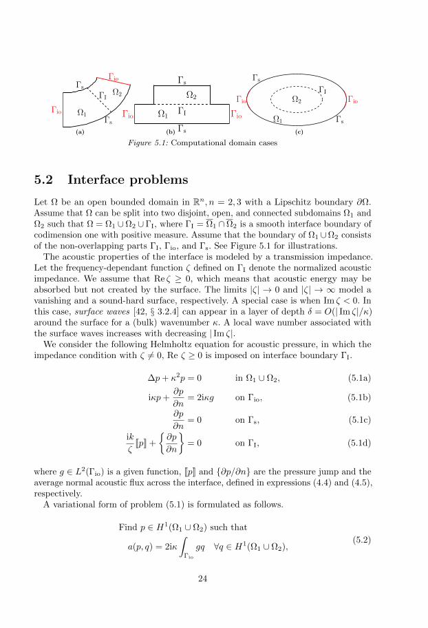
Let Ω be an open bounded domain in Rn, n = 2, 3 with a Lipschitz boundary ∂Ω.Assume that Ω can be split into two disjoint, open, and connected subdomains Ω1 andΩ2 such that Ω = Ω1 ∪Ω2 ∪ ΓI, where ΓI = Ω1 ∩Ω2 is a smooth interface boundary ofcodimension one with positive measure. Assume that the boundary of Ω1 ∪Ω2 consistsof the non-overlapping parts ΓI, Γio, and Γs. See Figure 5.1 for illustrations.

The acoustic properties of the interface is modeled by a transmission impedance.Let the frequency-dependant function ζ defined on ΓI denote the normalized acousticimpedance. We assume that Re ζ ≥ 0, which means that acoustic energy may beabsorbed but not created by the surface. The limits |ζ| → 0 and |ζ| → ∞ model avanishing and a sound-hard surface, respectively. A special case is when Im ζ < 0. Inthis case, surface waves [42, § 3.2.4] can appear in a layer of depth δ = O(| Im ζ|/κ)around the surface for a (bulk) wavenumber κ. A local wave number associated withthe surface waves increases with decreasing | Im ζ|.

We consider the following Helmholtz equation for acoustic pressure, in which theimpedance condition with ζ 6= 0, Re ζ ≥ 0 is imposed on interface boundary ΓI.

∆p+ κ2p = 0 in Ω1 ∪ Ω2, (5.1a)

iκp+∂p

∂n= 2iκg on Γio, (5.1b)

∂p

∂n= 0 on Γs, (5.1c)

ik

ζJpK +

∂p

∂n

= 0 on ΓI, (5.1d)

where g ∈ L2(Γio) is a given function, JpK and ∂p/∂n are the pressure jump and theaverage normal acoustic flux across the interface, defined in expressions (4.4) and (4.5),respectively.

A variational form of problem (5.1) is formulated as follows.

Find p ∈ H1(Ω1 ∪ Ω2) such that

a(p, q) = 2iκ

∫Γio

gq ∀q ∈ H1(Ω1 ∪ Ω2),(5.2)

24

where

a(p, q) =

∫Ω1∪Ω2

∇p · ∇q − κ2

∫Ω1∪Ω2

pq + iκ

∫Γio

pq + iκ

∫ΓI

1

ζJpKJqK. (5.3a)

In order for bilinear form a to be well defined on all of H1(Ω1 ∪Ω2)×H1(Ω1 ∪Ω2),we require that ζ ∈ L∞(ΓI) such that |ζ| ≥ δζ almost everywhere for some constantδζ > 0. With this condition, the existence of a unique solution for problem (5.2) canbe shown by using a Garding inequality and compactness [38, § 17.4].

The proposed finite element method for the interface problem, which seamlesslyhandles both vanishing and non-vanishing interface conditions, is as follows.

Find ph ∈ Vh such that

aλ(ph, qh) = `(qh) ∀qh ∈ Vh,(5.4)

where the space Vh of complex valued functions is as defined in Section 4.2 and

aλ(p, q) =

∫Ω1∪Ω2

∇p · ∇q − κ2

∫Ω1∪Ω2

pq −∫ΓI

∂p

∂n

(JqK +

ζ

iκ

∂q

∂n

)+

∫ΓI

ζ

iκ

∂p

∂n

∂q

∂n

−∫ΓI

(JpK +

ζ

iκ

∂p

∂n

)∂q

∂n

+

∫ΓI

λ

(JpK +

ζ

iκ

∂p

∂n

)(JqK +

ζ

iκ

∂q

∂n

)+ iκ

∫Γio

pq (5.5)

with a complex-valued function

λ =

(h

γ+ζ

iκ

)−1

(5.6)

for a sufficiently large γ > 0 and for mesh parameter h. Function λ is nonzero andbounded under the requirement

h Im ζ ≥ − γ

4κ|ζ|2 almost everywhere on ΓI. (5.7)

By construction the method is consistent and symmetric. The stability of the methodfollows from the following theorem. Let Γ−I be the union of all subsets of ΓI in whichIm ζ < 0 almost everywhere. Let U = L2(Ω1 ∪ Ω2)× L2(Γ−I ) and define the mappingJ : V → U by q 7→

(√κq, JqK

∣∣Γ−

I

/√δζ), which means that

‖Jq‖2U = κ

∫Ω1∪Ω2

|q|2 +1

δζ

∫Γ−

I

∣∣JqK∣∣2. (5.8)

We note that J is injective and compact with an image that is dense in U .

25

Theorem 5.2.1. Let λ be as defined above, let condition (5.7) holds, and let γ besufficiently large. Then, there is a constant Cc such that

|aλ(ph, qh)| ≤ Cc |||ph||| |||qh||| ∀ph, qh ∈ Vh ∪H2(Ω1 ∪ Ω2). (5.9)

Moreover, aλ satisfies

|aλ(ph, ph)|+ 2κ‖Jph‖2U ≥1

4||| ph |||2 ∀ph ∈ Vh, (5.10)

where

||| ph |||2 =

∫Ω1∪Ω2

|∇ph|2 + κ2

∫Ω1∪Ω2

|ph|2 +1

γ

∫ΓI

h∣∣∣ ∂ph

∂n

∣∣∣2 +

∫ΓI

|λ|∣∣JphK∣∣2. (5.11)

Assuming sufficient regularity of solutions to problem (5.2) and its dual, the followinga priori error estimate holds.

Theorem 5.2.2. Assume that ζ ∈ L∞(ΓI) satisfies |ζ| ≥ δζ > 0 almost everywhere onΓI. Let p be the solution of problem (5.2), assumed to satisfy p ∈ H1+σ(Ω1 ∪ Ω2) forsome σ ≥ 1, let ph be a solution to the discrete problem (5.4), and let k denote themaximal polynomial order of the elements in Vh. Then, there exists a mesh size limith1 > 0 and a constant C such that for each 0 < h ≤ h1,

||| p− ph ||| ≤ Chs|p|Hs+1(Ω1∪Ω2). (5.12)

where s = minσ, k.

5.3 Selected numerical results

Theorem 5.2.2 estimates the convergence rate of our method in the triple-norm. Tostudy the L2-convergence, we consider boundary value problem (5.1) in the domainΩ1 ∪ Ω2 = x ∈ R2 : 0 < |x1| < 1, 0 < x2 < 0.1 with an interface boundaryΓI = (0, x2) ∈ R2 : 0 < x2 < 0.1. Since Ω1 ∪ Ω2 is a narrow waveguide, the exactsolution is given by

p(x1, x2) =

e−iκ(x1+1) + ζ

2+ζ eiκ(x1−1) −1 < x1 < 0, 0 < x2 < 0.1

22+ζ e

−iκ(x1+1) 0 < x1 < 1, 0 < x2 < 0.1.(5.13)

Figure 5.2 shows the L2-convergence of the new and standard finite element methodsfor ζ = 0.21 + 0.10i. Note that the curves for the standard and new methods are ontop of each other. Numerical results also show that there is a similar convergence ratefor a vanishing interface, ζ = 0.

To observe the surface wave property, we solve boundary value problem (5.1) inΩ1 ∪ Ω2 ∈ R2, which is an arbitrary cross-section of a simple cylindrical reactivemuffler. Figure 5.3 shows the behaviour of the surface waves for varying bulk wavenumber κ and a fixed impedance ζ = −0.2i, whereas Figure 5.4 shows the behaviourfor a fixed wave number κ and a varying impedance.

26

-7 -6 -5 -4 -3 -2 -1 0-30

-25

-20

-15

-10

-5

0

5

∗+

♦×

∗+

♦×

∗

+

♦×

∗

+

♦×

∗

+

♦×

∗

+

♦×

∗

+

♦×

∗

+

♦×

∗

+

♦×

∗

+♦×

κ = 5

k = 1k = 2

k = 3♦♦♦

k = 1∗

k = 2+

k = 3×

log(h)

log(error)

-7 -6 -5 -4 -3 -2 -1 0-30

-25

-20

-15

-10

-5

0

5

∗+♦×

∗+

♦×

∗+

♦×

∗

+

♦×

∗

+

♦×

∗

+

♦×

∗

+

♦×

∗

+

♦×

∗

+

♦×

∗

+

♦× κ = 10

k = 1k = 2

k = 3♦♦♦

k = 1∗

k = 2+

k = 3×

log(h)

log(error)

-7 -6 -5 -4 -3 -2 -1 0-30

-25

-20

-15

-10

-5

0

5

∗+♦×∗+♦×∗+♦×∗+♦×

∗+

♦×

∗

+

♦×

∗

+

♦×

∗

+

♦×

∗

+

♦×

∗

+

♦×

κ = 50

k = 1k = 2

k = 3♦♦♦

k = 1∗

k = 2+

k = 3×

log(h)

log(error)

-7 -6 -5 -4 -3 -2 -1 0-30

-25

-20

-15

-10

-5

0

5

∗+♦×∗+♦×∗+♦×∗+♦×∗+♦×

∗+

♦×

∗

+

♦×

∗

+

♦×

∗

+

♦×

∗

+

♦×

κ = 100

k = 1k = 2

k = 3♦♦♦

k = 1∗

k = 2+

k = 3×

log(h)

log(error)

Figure 5.2: Convergence rates of the standard finite element and the proposed method forthe interface problem with acoustic impedance ζ = 0.21 + 0.10i for polynomial orders k = 1,k = 2, and k = 3, and wave numbers κ = 5, κ = 10, κ = 50, and κ = 100. The dotted lines

are reference lines for second, third, and fourth order L2-convergence.

κ = 10 κ = 20

κ = 40 κ = 80

Figure 5.3: Surface waves corresponding to different wave numbers for ζ = −0.2i.

ζ = −0.2i ζ = −0.1i

ζ = −0.05i ζ = −0.025i

Figure 5.4: Surface waves behaviour as Im(ζ) varies for κ = 10.5.

27

Chapter 6

Summary of Paper III and Paper IV -

Layout optimization of thin sound-hard

material to improve the far-field directivity

properties of an acoustic horn

6.1 Introduction

In the material distribution to topology optimization [12], a design region is dividedinto a large number of small elements (“pixels” in 2D and “voxels” in 3D), andthe optimization algorithm decides about the material composition of each element.The material distribution approach [12] is usually associated with techniques such asrelaxation, penalization, and design filters to obtain mesh independent designs. Thisapproach has the tendency to produce designs with extended volumes of materialand to filter out thin structures. However, numerical experiences with optimizationof devices for acoustic wave propagation have indicated a propensity for creation ofthin (for example see Paper I) and scattered [43] structures, which are difficult toaccomplish with the traditional topology optimization approach.

In Paper III, a material distribution approach to determine the layout of thinmaterials inside an acoustic horn is introduced. The acoustic properties of thinmaterials are modeled by an acoustic transmission impedance. We use the finiteelement method introduced in Chapter 5 to handle both vanishing and non-vanishingsurface impedance simultanuously.

Paper IV outlines some technical details in connection to the problem treatedin Paper III. In particular, it presents matrix representation for evaluations of thefar-field pattern and the sensitivity analysis of the problem. We use the adjoint-basedmethod [44, § 6] to efficiently compute the gradient of the objective function withrespect to the design variables, and the accuracy of the gradient computation is verifiedagainst finite difference approximations.

29

Incoming plane wave

Outgoing wave

2a 2b

ldz′

y′

x′

(a)

RΩ

Γout

Γin

ΩA

ΩW ΩH

Γs

Γsym

(b)

Figure 6.1: The horn to be optimized and the computational domain.

6.2 Problem description

We consider a cylindrically symmetric horn as shown in Figure 6.1a. The shape ofthe horn has already been determined by shape optimization aiming for a perfecttransmission by minimizing the reflections of the horn back to its throat [45]. For thepurpose of numerical computations, using the axial symmetry assumption, the exteriordomain is truncated by an artificial far-field boundary Γout, which yields a boundeddomain Ω, as depicted in Figure 6.1b. We assume that Ω is the union of three disjoint,open, and connected subdomains ΩW, ΩH, and ΩA, that is, Ω = ΩW ∪ ΩH ∪ ΩA. Theboundaries of the computational domain are denoted by Γout; Γin, the left boundary ofthe truncated waveguide; Γsym, an axial symmetry line; and Γs, the boundary betweensound-hard material and air.

Assume that the wave propagation is governed by the wave equation for the acousticpressure P . By seeking a time harmonic solution, the time varying pressure field isseparated as P (x, t) = R(p(x)eiωt), where R is the real part, p is a complex amplitudefunction, ω is the angular frequency, x = (r, z), and i2 = −1. The amplitude functionp satisfies the Helmholtz equation

1

r∇ · (r∇p) + κ2p = 0 in Ω, (6.1)

where κ = ω/c is the wavenumber, r is the radial coordinate, and ∇ = (∂/∂r, ∂/∂z).Assume that the incoming wave at the inlet boundary Γin is a plane wave of

amplitude A. The first order Engquist–Majda absorbing boundary condition is used toapproximate the Sommerfeld radiation condition on Γout [46, 47]. Then, the complexamplitude function satisfies(

iκ+1

RΩ

)p+

∂p

∂n= 0 on Γout, (6.2a)

iκp+∂p

∂n= 2iκA on Γin, (6.2b)

∂p

∂n= 0 on Γs ∪ Γsym. (6.2c)

30

To improve the performance of the given horn, we aim to distribute thin sheets ofsound-hard material along a grid inside ΩH. These squares partition the computationaldomain into several small subdomains and introduce numerous interface boundariesbetween the subdomains. We denote the union of all interface boundaries by ΓI anddefine Ω0 = Ω \ ΓI.

By assuming that the flux of the acoustic pressure is continuous over the interface,we have (see Section 2.1 of Paper II for the derivation)

ik

ζJpK +

∂p

∂n

= 0 on ΓI, (6.3)

where ζ is the normalized transition impedance, and JpK and ∂p/∂n are the pressurejump and the average normal acoustic flux across the interface, respectively. Notethat the limits |ζ| → 0 and |ζ| → ∞ model a vanishing and a sound-hard surface,respectively.

Helmholtz equation (6.1), together with boundary conditions (6.2) and interfacecondition (6.3), yields the following variational problem.

Find p ∈ H1(Ω0) such that

a(p, q) := a0(p, q) + iκ

∫ΓI

r

ζJpKJqK = 2iκA

∫Γin

rq ∀q ∈ H1(Ω0), (6.4)

where

a0(p, q)=

∫Ω0

r∇p · ∇q−κ2

∫Ω0

rpq + iκ

∫Γin∪Γout

rpq +1

RΩ

∫Γin

rpq. (6.5)

We characterize the structure of ΓI by a material indicator function α : ΓI → 0, 1defined such that α(x) = 0 if x is occupied by material and α(x) = 1 if x is occupiedby air. Then, we define the impedance function ζ such that ζ = 0 when α = 1, thatis, for a vanishing interface, and such that ζ attains a large, purely imaginary valuewhen α = 0, that is, when approximating the impedance of a sound-hard material. Toenable the use of gradient-based optimization algorithm, we relax the design variable,α to attain any value in the range [0, 1].

We introduce a collection of non-degenerate triangulationsT hih>0

of the subdo-

mains Ωi. Let V hi be the space of all complex-valued continuous functions that arebi-quadratic polynomials on each element in Ωi and extended by zero into Ω \ Ωi. Wedefine the finite element space by Vh =

∑i V

hi . The solution of the acoustic problem

p ∈ H1(Ω0) is approximated in the space Vh and denoted by ph. The material indicatorfunction α is approximated by an edge-wise constant function αh : ΓI → [0, 1] andimpedance function ζ is approximated by the edge-wise constant function ζh = ζ(αh).

Based on a Nitsche-type formulation introduced in Chapter 5, the discrete variationalproblem which handles both vanishing and non-vanishing interface conditions is definedas follows.

Find ph ∈ Vh such that

aλ(ph, qh) = `(qh) ∀qh ∈ Vh,(6.6)

31

where the discrete bilinear form aλ is defined by

aλ(ph, qh) = a0(ph, qh)−∫ΓI

(1− λζhiκ

)(JqhK

∂ph∂n

+JphK

∂qh∂n

)

−∫ΓI

ζhiκ

(1− λζh

iκ

)∂ph∂n

∂qh∂n

+

∫ΓI

λJphKJqhK, (6.7)

in which the function λ ∈ L∞(ΓI) is as defined in expression (5.6).

6.3 Optimization problem

The objective of the optimization is to improve the far-field performance of the referencehorn shown in Figure 6.1a while keeping the efficiency of the new design as high aspossible. For single frequency f and a given design αh, to minimize the reflection andthe difference in magnitude of the far-field intensities at two given angles θ1 and θ2,we consider the objective functions

Jhr (αh; f) =1

2|〈ph〉Γin

−A|2, (6.8a)

Jh∞(αh; f, θ1, θ2) =1

2

∣∣∣ log10

( |ph,∞(θ1)|2|ph,∞(θ2)|2

)∣∣∣, (6.8b)

where 〈·〉Γin is the mean acoustic pressure over Γin as defined in expression (3.6), andph is the solution of problem (6.6) for a κ = 2πf/c and ζh = iζmax(1 − αh)3; ζmax

is chosen such that ζh = iζmax approximates the impedance of sound-hard material.Here the far-field pattern at an angle θ is defined by

ph,∞(θ) =1

4π

∫Γout

eiκx·x(

1

RΩ+ iκ+ iκx · n

)ph, (6.9)

where x(θ) is a point on the unit sphere at an angle θ with respect to the symmetryaxis. Then, the objective function used for the optimization is given by

Jh(αh;F ,Θ) =1

nf

nf∑i=1

Jhr (αh; fi) +1

nf (nθ−1)

nf∑i=1

nθ−1∑j=1

Jh∞(αh, fi, θj , θj+1), (6.10)

where F = f1, f2, . . . , fnf and Θ = θ1, θ2, . . . , θnθ are the set of consideredfrequencies and angles, respectively. The set of feasible designs is defined by

Uh =αh ∈ L∞(ΓI) : 0 ≤ αh ≤ 1 a.e. in ΓI

. (6.11)

32

6.4 Sensitivity Analysis

Let ai denote the value of the piecewise constant functions αh on boundary meshelement Ei in ΓI, and define the vector representation of αh by a = (a1, . . . , aNΓ

)T ,where NΓ is the number of interface boundary elements. For a single frequency f andangles θ1 and θ2, consider the objective function

Jh(a; f, θ1, θ2) =1

2log10

( |ph,∞(θ1)|2|ph,∞(θ2)|2

). (6.12)

The derivative of Jhwith respect to ai, using the chain rule and the adjoint-basedcomputation, is (see Paper IV for the full derivation)

∂J(a; f, θ1, θ2)

∂ai=G(θ1)−G(θ2)

ln(10), (6.13)

where

G(θ) =1

|ph,∞(θ)|2

(Rph,∞(θ)R

∂ph,∞(θ)

∂ai

+ Iph,∞(θ)I

∂ph,∞(θ)

∂ai

). (6.14)

Here,

∂ph,∞∂ai

=

∫Ei

dc1dai

r

(JzhK

∂ph∂n

+ JphK

∂zh∂n

)+

∫Ei

dc2dai

r

∂zh∂n

∂ph∂n

−∫Ei

dλ

dairJzhKJphK,

(6.15)

withdλ

dai= − 1

iκλ2i

dζh,idai

,

dc1dai

= − 1

iκ

(λi −

1

iκλ2i ζh,i

)dζh,idai

,

dc2dai

=1

iκ

(1− ζh,i

iκ

(2λi −

1

iκλ2i ζh,i

)) dζh,idai

,

(6.16)

where λi = λ|Ei , ζh,i = ζh(ai) and zh is the solution to the following adjoint problem.

Find zh ∈ Vh such that

aλ(αh; vh, zh) = vh,∞(θ) ∀vh ∈ Vh,(6.17)

where

vh,∞(θ) =1

4π

∫Γ3d

out

eiκx·x(

1

RΩ+ iκ+ iκx · n

)vh. (6.18)

Note that the derivative dζh,i/dai in expression (6.16) depends on the parametrizationof ζh,i. The accuracy of the gradient computation in expression (6.13) is verified againstfinite difference approximations in Paper IV.

33

(a) (b)

Figure 6.2: Final horn designs: (a) optimized for three target frequencies 6400× 2(m−2)/12 Hz,for m = 0, 1, 2 and (b) optimized for nine target frequencies 6400 × 2(m−2)/12 Hz, 0, 1, . . . , 8.

Frequency (Hz)1500 2500 3500 4500 5500 6500 7500 8500 9500

Bea

m W

idth

(°)

40

50

60

70

80

90

100

110

120

130

140Design 1Design 2Ref. horn

(a)

Frequency (Hz)0 1000 2000 3000 4000 5000 6000 7000 8000 9000 10000

|R|

0

0.1

0.2

0.3

0.4

0.5

0.6

0.7

0.8

0.9

1Design 1Design 2Ref. horn

(b)

Figure 6.3: The beam width and reflection spectrum as functions of frequency of the optimzedhorns in Figure 6.2 and the reference horn. Design 1 and Design 2 refer to the designs in

Figures 6.2a and 6.2b, respectively, and Ref. Horn is the reference horn.

6.5 Selected numerical results

We consider the reference horn depicted in Figure 6.1a with length l = 161.5 mm,throat radius a = 19.3 mm, and mouth radius b = 150 mm. The waveguide has aradius of a = 19.3 mm and a length of d = 206.5 mm. The horn region ΩH, illustratedin Figure 6.1b, is divided into 68 subdomains by putting 67 squares with side length8.9722 mm. The boundaries between the subdomains form the interface ΓI consistingof 146 components. The reference horn has virtually perfect transmission propertieswithin the considered frequency range. The reflection spectrum of the reference horn isplotted in Figure 6.3b (dashed line). However, the far-field properties of the referencehorn are not ideal, in particular for higher frequencies. The beam width of the referencehorn is plotted in Figure 6.3b (dashed line). We optimize the horn for an even far-fielddirectivity at angles 0, 5, 10, 15, 20, and 25 with respect to the symmetry axis.

Figures 6.2a and 6.2b show the final designs of the horn optimized for three targetfrequencies 6400 × 2(m−2)/12 Hz, for m = 0, 1, 2 and nine target frequencies 6400 ×2(m−2)/12 Hz, 0, 1, . . . , 8, respectively. Figure 6.3a shows the beam width of the twooptimized designes depicted in Figure. 6.2 using the dash-dotted and solid lines,respectively. The beam width for the two designs are uniformly above 60 in frequencyband 1600 to 9050 Hz. The reflection spectra of the designs in Figures 6.2a and 6.2band the reference horn are shown in Figure 6.3b.

34

Chapter 7

Summary of Paper V - State constrained

optimal control of a ball pitching robot

7.1 Introduction

In Paper V, we study an optimal control problem of a ball pitching robot that isdesigned to capture important dynamics of the human upper limb (including theshoulder, arm, and forearm) during an overarm throw. The robot has two links thatare connected at the elbow joint by a linear torsional spring. The links represent thearm and forearm, and the spring represents the stiffness of the muscles around theelbow joint in human upper limb [48, 49]. The two-link robot is connected to a motorshaft at the shoulder joint by a non-linear torsional spring. At the end of the forearm,the robot is equipped with a gripping mechanism that allows the robot to grasp andrelease the ball at any required time.

The main objective is to determine the optimal motor torque and the release timethat enable the robot to pitch the ball as far as possible. We include constraints onthe motor torque and power as well as the angular velocity of the motor shaft intothe problem formulation. For computational efficiency, we replace the time-globalconstraints on maximum allowed power and maximum angular velocity of the motorshaft by approximations based on integral quantities.

7.2 Problem formulation

The initial configuration of the two-link robot with a gripping mechanism holdinga ball is illustrated in Figure 7.1. We denote the two links by the arm and forearm,respectively. Let q2 measure the angle change between the arm and the forearm atthe elbow joint. The angles q1 and qm, measured with respect to the horizontal axis,describe the configuration of the arm and the motor shaft, respectively. The onlydriving force of the system comes from the motor shaft. Figure 7.2 shows a trajectory

35

x

y

m1

m2

xr

releaseline

qmq1

−q2

τm

mb

1

Figure 7.1: Initial configuration of thepitching robot and the release line.

x

y

xr

t = trvb

τm

1Figure 7.2: Configuration of the pitchingrobot at the release time and the balltrajectory during the pitching motion.

of the ball during a pitching motion. The ball gets released with velocity vb in thedesired direction when it crosses the release line (x, y) = (xr, s), s ∈ R.

Let q = [qm, q1, q2]T be a vector of generalized coordinates of the robotic manipulator,and let θ(t) = [q(t), q(t)]T ∈ R6 be the state vector. Let τ(t) ∈ R be a variable thatmeasures the torque of the motor. The equations of motion of the system, derivedbased on the Euler–Lagrange formulation in Appendix A of Paper V, in state spacerepresentation becomes

θ = f(θ, τ), (7.1)

where,

f(θ, τ) =

θ4

θ5

θ6

I−1m (τ − τs(θ))

M(θ)−1

(K(θ)−G(θ)− C(θ)

[θ4

θ5

])

, (7.2)

and where, Im is the motor inertia, τs(θ) the torque due to the non-linear spring at theshoulder joint, M(θ) the inertia matrix, C(θ) the matrix of centrifugal and Coriolisforces, and where the vectors G(θ) and K(θ) represent gravitational and spring forces,respectively.

As illustrated in Figure 7.2, at time t = tr the ball is released with velocity vb. Itthen follows a ballistic trajectory until it hits the ground at a point (J, 0), where

J(θ, xr) = xr +xb(tr)

g

(yb(tr) +

√yb(tr)2 + 2gyb(tr)

). (7.3)

Here xr is the position of the vertical release line (x, y) = (xr, s), s ∈ R, at which thegripping mechanism of the robot releases the ball, and g is the gravitational constant.

36

The vertical position of the ball at the release time is

yb(tr) = l1 sin(q1(tr)) + l2 sin(q1(tr) + q2(tr)),

where l1 and l2 are the lengths of the arm and the forearm, respectively. Similarly, thevelocity of the ball vb = (xb, yb) at time t = rr is given by

xb(tr) = −l1 sin(q1(tr))q1(tr)− l2 sin(q1(tr) + q2(tr))(q1(tr) + q2(tr)),

yb(tr) = l1 cos(q1(tr))q1(tr) + l2 cos(q1(tr) + q2(tr))(q1(tr) + q2(tr)).(7.4)

Note that the robot’s shoulder is held fixed at the origin of the coordinate systemand that the ball is thrown in the negative x direction. Hence, minimizing J impliesmaximizing the distance between the origin and the point (J, 0).

We minimize J over the torque change in time. By inclusion of the constraints onthe motor torque and torque change in the set of admissible controls, we obtain

A =

η ∈ L∞ | sup

t|η(t)| ≤ Cτ , sup

t

∣∣∣∣τ0 +

∫ t

0

η(s) ds

∣∣∣∣ ≤ τ , (7.5)

where τ is the maximum allowed torque of the motor, Cτ is the bound on the torquechange in time, and η is the our control function defined by

τ = η,

τ(0) = τ0.(7.6)

For computational efficiency, we replace the time-global constraints on maximumallowed power and maximum angular velocity of the motor shaft by approximationsbased on integral quantities (see Paper V for further discussion). For practical reasons,we impose the constraint |xr| ≤ l1 + l2 on the release line. Since it is possible todetermine the release line position if the release time is known and vice versa, weoptimize with respect to the release line position instead of the time.

Putting the system dynamics, the objective function, and the constraints together,we obtain the optimal control problem

minη∈A,

|xr|≤l1+l2

J(xr, θ(tr))

subject to τ = η, τ(0) = τ0,

θ = f(θ, τ), θ(0) = θ(0),(1

tr

∫ tr

0

|θ4|p dt

)1/p

≤(

1

p+ 1

)1/p

Qmax,(1

tr

∫ tr

0

|τθ4|p dt

)1/p

≤(

1

p+ 1

)1/p

Pmax,

(7.7)

where Qmax and Pmax are the maximum allowed angular velocity of the motor shaftand input power of the motor, respectively, and θ(0) is the initial state of the system.

37

Time [s]0 0.2 0.4 0.6 0.8

Moto

rto

rque

[Nm

]

-50

0

50

100

-0.5 0 0.5 1-0.6

-0.4

-0.2

0

0.2

0.4

0.6

0.8

Figure 7.3: Left: the time evaluation of the optimal torque. Right: the ball trajectory duringthe pitching motion, starting from the initial position up to the time when the ball is released.

To numerically solve optimal control problem (7.7), we use a uniform discretizationof the time interval [0, T ], where T is a sufficiently large time such that 0 < tr ≤ T .Then, we use the so-called Heun’s method to numerically solve the state equation. Thediscrete version of optimal control problem (7.7) is solved numerically by an interiorpoint method with BFGS Hessian approximation as implemented in Matlab’s fmincon.The gradients of the objective function and the constraint function is computed bythe discrete adjoint approach.

7.3 Selected numerical results

The non-linear spring at the shoulder joint produces a torque that is approximated bythe function

τs = 7761.7(qm − q1)3 + 2.9755(qm − q1)2 + 77.8080(qm − q1)− 0.0334. (7.8)

The coefficients are obtained from a least-squares fit with measured data, for the ballpitching robot we study, in the range |qm − q1| ≤ 0.25 rad. In this range, the relativeerror between the measured data and the cubic model is less than 2.5 × 10−3. Theinitial conditions

q0 = [0.978, 0.908,−0.172] rad∗, q0 = 0 rad/s, and τ0 = 8.213 Nm (7.9)

are determined in such away that the system is stationary at time t0 = 0 for a givenq1(0) = π − 2.234 rad. The lengths of the arm and the forearm are l1 = 0.3 m and

∗In the published paper, the order of the elements in q0 is erroneous.

38

Time [s]0 0.2 0.4 0.6 0.8

Angl

e[rad]

-2

-1

0

1

qm q1 q2

Time [s]0 0.2 0.4 0.6 0.8

Angu

larve

locity

[rad/s

]

-20

-10

0

10

_qm _q1 _q2

Figure 7.4: Time evolution of the generalized coordinates q1, q2, and qm (left),the corresponding angular velocities q1, q2 and qm (right) computed using the

optimal input torque from Figure 7.3.

l2 = 0.542 m, respectively. The maximum allowed motor torque, power and angularvelocity of the motor shaft are τ = 180 Nm, Pmax = 270 Nm/s and Qmax = 3.787 rad/s,respectively. For a complete set of parameters for this experiment refer to Paper V.We set T = 2 s, ∆t = 0.0025 s, Cτ = 1000 Nm/s, and p = 100 for the numericalexperiments.

Figure 7.3 shows the time evaluation of the resulting optimal input torque profile(left diagram) and the ball trajectory during the pitching motion (right diagram). Thetorque profile shows that the optimal torque attains its maximum value 89.54 Nmafter 0.473 s. The optimal release line given by (x, y) = (xr, s), where xr = 0.506 mand s ∈ R, and the pitching motion takes tr = 0.843 s to cross the release line. Theball is thrown at an upward angle of 40.82 degrees with velocity of 11.36 m/s. Afterthe ball is released, it follows a ballistic trajectory in the negative direction and finallyhits the ground 13.25 m away from the origin (the robot’s shoulder position).

Figure 7.4 illustrates the time evolution, from the initial time to the final time, ofthe generalized coordinates q1, q2, and qm (left diagram), and the angular velocitiesq1, q2, and qm (right diagram). Recall that q2 measures the angle change between thearm and the forearm, while q1 and qm measure the angle of the arm and the motorshaft with respect to the horizontal line. The left diagram illustrates, in particular,that |qm − q1| ≤ 0.25 rad throughout the motion.

From the right diagram of Figure 7.4, we can see that the angular velocity qm of themotor shaft (solid line) essentially has four phases. Starting from a stationary position,in the first phase it decelerates from a stationary position until it reaches an angularvelocity of about −3.7 rad/s. The motor shaft moves at an almost constant angularvelocity in the second phase, and accelerates rapidly in the third phase. Finally, themotor shaft moves at a relatively constant angular velocity of about 3.7 rad/s. Inthe second and last phase the angular speed qm of the motor shaft reached to the

39

Figure 7.5: Snapshots of the ball pitching robot during the throwing motion obtained byusing the optimal input torque presented in Figure 7.3. The snapshots are taken at times(top row from left to right) t = 0, tr/7, 2tr/7, and 3tr/7 and (bottom row from left to right)t = 4tr/7, 5tr/7, 6tr/7, and tr, where tr = 0.843 s is the duration of the throwing motion.

maximum bound. During the last 0.35 s, the angular velocity, q1 + q2 of the forearmmeasured with respect to the horizontal line is strictly increasing.

Figure 7.5 shows snapshots, taken at equal time interval, of the robot and illustratesthe trajectory of the ball during the throwing motion. The snapshots suggest thatabout three quarters of the total pitching time is spent on swinging the ball backwardagainst the throwing direction to get longer interval of acceleration. In the last quarterof the pitching time, the arm and forearm swings forward to the direction of the throwand the ball accelerates rapidly and reaches its maximum velocity at the release.

40

Bibliography

[1] D.E. Kirk. Optimal Control Theory: An Introduction. Dover Books on ElectricalEngineering Series. Dover Publications, 2004.

[2] K. Svanberg. The method of moving asymptotes–a new method for structural opti-mization. International Journal for Numerical Methods in Engineering, 24(2):359–373, 1987.

[3] M.P. Bendsøe and N. Kikuchi. Generating optimal topologies in structural designusing a homogenization method. Computer Methods in Applied Mechanics andEngineering, 71(2):197–224, 1988.

[4] O. Sigmund. Tailoring materials with prescribed elastic properties. Mechanics ofMaterials, 20(4):351–368, 1995.

[5] S. Zhou and Q. Li. Design of graded two-phase microstructures for tailoredelasticity gradients. Journal of Materials Science, 43:5157–5167, 2008.

[6] K. E. Jensen, P. Szabo, and F. Okkels. Topology optimization of viscoelasticrectifiers. Applied Physics Letters, 100(23):234102–234102–3, 2012.

[7] T. Borrvall and J. Petersson. Large-scale topology optimization in 3d usingparallel computing. Computer Methods in Applied Mechanics and Engineering,190(46-47):6201–6229, 2001.

[8] H. Guan, Y.J. Chen, Y.C. Loo, Y.M. Xie, and G.P. Steven. Bridge topologyoptimization with stress, displacement and frequency constraints. Computers andStructures, 81(3):131–145, 2003.

[9] L. Wang, P.K. Basu, and J.P. Leiva. Automobile body reinforcement by finiteelement optimization. Finite Elements in Analysis and Design, 40(8):879–893,2004.

[10] L. Krog, A. Tucker, M. Kemp, and R. Boyd. Topology optimization of aircraftwing box ribs. In 10th AIAA/ISSMO Multidisciplinary Analysis and OptimizationConference, page 16, 2004.

41

[11] O. Sigmund and J. Petersson. Numerical instabilities in topology optimization: Asurvey on procedures dealing with checkerboards, mesh-dependencies and localminima. Structural optimization, 16:68–75, 1998.

[12] M.P. Bendsøe and O. Sigmund. Topology optimization. Theory, methods, andapplications. Springer, 2003.

[13] O. Sigmund. A 99 line topology optimization code written in matlab. Structuraland Multidisciplinary Optimization, 21(2):120–127, 2001.

[14] C.S. Jog and R.B. Haber. Stability of finite element models for distributed-parameter optimization and topology design. Computer Methods in AppliedMechanics and Engineering, 130(3–4):203–226, 1996.

[15] T. Borrvall and J. Petersson. Topology optimization using regularized intermediatedensity control. Computer Methods in Applied Mechanics and Engineering, 190(37-38):4911–4928, 2001.

[16] M.P. Bendsøe. Optimal shape design as a material distribution problem. Structuraland Multidisciplinary Optimization, 1(4):193–202, 1989.

[17] A. Rietz. Sufficiency of a finite exponent in SIMP (power law) methods. Structuraland Multidisciplinary Optimization, 21(2):159–163, 2001.

[18] A. D´iaz and O. Sigmund. Checkerboard patterns in layout optimization. Struc-tural optimization, 10:40–45, 1995.

[19] O. Sigmund. Morphology-based black and white filters for topology optimization.Structural and Multidisciplinary Optimization, 33(4-5):401–424, 2007.

[20] O. Sigmund. Design of Material Structures Using Topology Optimization. PhDthesis. Technical University of Denmark, 1994.

[21] T.E. Bruns and D.A. Tortorelli. Topology optimization of non-linear elasticstructures and compliant mechanisms. Computer Methods in Applied Mechanicsand Engineering, 190:3443–3459, 2001.

[22] B. Bourdin. Filters in topology optimization. International Journal for NumericalMethods in Engineering, 50(9):2143–2158, 2001.

[23] M.Y. Wang and S. Wang. Bilateral filtering for structural topology optimization.International Journal for Numerical Methods in Engineering, 63(13):1911–1938,2005.

[24] L. Munjal. Acoustics of ducts and mufflers with application to exhaust andventilation system design. Wiley-Interscience publication. Wiley, 1987.

[25] T.W. Wu and G.C. Wan. Muffler performance studies using a direct mixed–bodyboundary element method and a three-point method for evaluating transmissionloss. Journal of Vibration and Acoustics, 118(3):479–484, 1996.

42

[26] D.D. Davis, G.M. Stokes, D. Moore, and G.L. Stevens. Theoretical and experi-mental investigation of mufflers with comments on engine-exhaust muffler design.NACA report 1192, 1954.

[27] J. Nitsche. Uber ein Variationsprinzip zur Losung von Dirichlet-Problemen beiVerwendung von Teilraumen, die keinen Randbedingungen unterworfen sind.Abhandlungen aus dem Mathematischen Seminar der Universitat Hamburg, 36:9–15, 1971.

[28] I. Babuska. The finite element method with Lagrange multiplayer. NumerischeMathematik, 20(122):179–192, 1973.

[29] H.J.C. Barbosa and T.J.R. Hughes. The finite element method with Lagrange mul-tipliers on the boundary: circumventing the Babuska-Brezzi condition. ComputerMethods in Applied Mechanics and Engineering, 85(1):109 – 128, 1991.

[30] H.J.C. Barbosa and T.J.R. Hughes. Boundary Lagrange multipliers in finiteelement methods: Error analysis in natural norms. Numerische Mathematik,62(1):1–15, 1992.

[31] R. Stenberg. On some techniques for approximating boundary conditions in thefinite element method. Journal of Computational and Applied Mathematics, 63(1- 3):139 – 148, 1995.

[32] M. Juntunen and R. Stenberg. Nitsche’s method for general boundary conditions.Mathematics of Computation, 78(267):1353–1374, 2009.

[33] D.N. Arnold. An interior penalty finite element method with discontinuouselements. SIAM Journal on Numerical Analysis, 19(4):742–760, 1982.

[34] D.N. Arnold, F. Brezzi, B. Cockburn, and L.D. Marini. Unified analysis ofdiscontinuous Galerkin methods for elliptic problems. SIAM Journal on NumericalAnalysis, 39(5):1749–1779, 2002.

[35] R. Stenberg. Mortaring by a method of J. A. Nitsche. Computational Mechanics,New Trends and Applications, pages 1–6, 1998.

[36] R. Becker, P. Hansbo, and R. Stenberg. A finite element method for domaindecomposition with non-matching grids. ESAIM Mathematical Modelling andNumerical Analysis, 37(2):209–225, 2003.

[37] A. Hansbo and P. Hansbo. An unfitted finite element method, based on Nitsche’smethod, for elliptic interface problems. Computer Methods in Applied Mechanicsand Engineering, 191(47-48):5537–5552, 2002.

[38] J. Wloka. Partial Differential Equations. Cambridge University Press, 1987.

[39] S.C. Brenner and R. Scott. The Mathematical Theory of Finite Element Methods.Texts in Applied Mathematics. Springer, 2008.

43

[40] P.G. Ciarlet. The Finite Element Method for Elliptic Problems. Society forIndustrial and Applied Mathematics, Philadelphia, PA, USA, 2002.

[41] A. Hansbo and P. Hansbo. A finite element method for the simulation of strongand weak discontinuities in solid mechanics. Computer Methods in AppliedMechanics and Engineering, 193(33–35):3523–3540, 2004.

[42] S.W. Rienstra and A. Hirschberg. An introduction to acoustics. Revised andupdated version of reports IWDE 92-06 and IWDE 01-03, Eindhoven Universityof Technology, 2015.

[43] E. Wadbro, R. Udawalpola, and M. Berggren. Shape and topology optimizationof an acoustic horn–lens combination. Journal of Computational and AppliedMathematics, 234(6):1781–1787, 2010.

[44] P.W. Christensen and A. Klarbring. An Introduction to Structural Optimization,volume 153 of Solid Mechanics and Its Applications. Springer, 2008.

[45] D. Noreland, R. Udawalpola, P. Seoane, E. Wadbro, and M. Berggren. An efficientloudspeaker horn designed by numerical optimization: An experimental study.Report UMINF 10.1, Department of Computing Science, Umea University, 2010.

[46] B. Engquist and A. Majda. Absorbing boundary conditions for the numericalsimulation of waves. Mathematics of Computation, 31(139):629 –651, 1977.

[47] F. Ihlenburg. Finite Element Analysis of Acoustic Scattering. Springer, NewYork, 1998.

[48] S. Katsumata, S. Ichinose, T. Shoji, S. Nakaura, and M. Sampei. Throwing motioncontrol based on output zeroing utilizing 2-link underactuated arm. In Proceedingsof the 2009 conference on American Control Conference, pages 3057–3064, 2009.

[49] U. Mettin, A.S. Shiriaev, L.B. Freidovich, and M. Sampei. Optimal ball pitchingwith an underactuated model of a human arm. In IEEE International Conferenceon Robotics and Automation, ICRA 2010, pages 5009–5014, 2010.

44