analysis of an interface stabilised finite element method

arX

iv:1

010.

1873

v2 [

mat

h.N

A]

31

Mar

201

1

ANALYSIS OF AN INTERFACE STABILISED FINITE ELEMENT

METHOD: THE ADVECTION-DIFFUSION-REACTION EQUATION

GARTH N. WELLS∗

Abstract. Analysis of an interface stabilised finite element method for the scalar advection-diffusion-reaction equation is presented. The method inherits attractive properties of both continuousand discontinuous Galerkin methods, namely the same number of global degrees of freedom as a con-tinuous Galerkin method on a given mesh and the stability properties of discontinuous Galerkinmethods for advection dominated problems. Simulations using the approach in other works demon-strated good stability properties with minimal numerical dissipation, and standard convergence ratesfor the lowest order elements were observed. In this work, stability of the formulation, in the formof an inf-sup condition for the hyperbolic limit and coercivity for the elliptic case, is proved, as isorder k + 1/2 order convergence for the advection-dominated case and order k + 1 convergence forthe diffusive limit in the L2 norm. The analysis results are supported by a number of numericalexperiments.

Key words. Finite element methods, discontinuous Galerkin methods, advection-diffusion-reaction

AMS subject classifications. 65N12, 65N30

1. Introduction. Discontinuous Galerkin methods have proven effective andpopular for classes of partial differential equations, in particular transport equa-tions in which advection is dominant. The attractive stability properties of suitablyconstructed discontinuous Galerkin methods and the possibility of matching non-conforming meshes are advantageous, but do come at the cost of an increased num-ber of global degrees of freedom on a given mesh compared to continuous Galerkinmethods. In a number of recent works, advances have been made in reconciling theappealing features of continuous and discontinuous Galerkin methods in one frame-work. Works in this direction include those of Hughes et al. [1], Labeur and Wells [2]and Cockburn et al. [3] for the advection-diffusion equation, Burman and Stamm [4]for advection-reaction equation, and Labeur and Wells [2] and Labeur and Wells [5]for the incompressible Navier-Stokes equations. These methods generally strive for areduction in the number of global degrees of freedom relative to a conventional dis-continuous Galerkin method without sacrificing other desirable features. In this work,stability and convergence estimates are presented for one such method applied to thescalar advection-diffusion-reaction equation, namely the interface stabilised methodas formulated in Labeur and Wells [2].

The principle behind the interface stabilised method is simple: the equation ofinterest is posed cell-wise subject to weakly imposed Dirichlet boundary conditionsin the spirit of discontinuous Galerkin methods. The boundary condition which isweakly satisfied is provided by an ‘interface’ function that lives only on cell facetsand is single-valued on cell facets. An equation for this additional field is furnishedby insisting upon weak continuity of the so-called ‘numerical flux’ across cell facets.This weak continuity of the numerical flux is in contrast with typical discontinuousGalerkin methods which satisfy continuity of the numerical flux across cell facetspoint-wise by construction. For particular choices in the method, it may be possibleto achieve point-wise continuity. Upwinding of the advective flux at interfaces can

∗Department of Engineering, University of Cambridge, Trumpington Street, Cambridge CB2 1PZ,United Kingdom ([email protected]).

1

http://arxiv.org/abs/1010.1873v2

2 GARTH N. WELLS

be incorporated naturally in the definition of the numerical flux, as is typical fordiscontinuous Galerkin methods. By building a degree of continuity into the interfacefunction spaces (at cell vertices in two dimensions and across cell edges in threedimensions), the number of global degrees of freedom is equal to that for a continuousGalerkin method on the same mesh. The key to this reduction in the number of globaldegrees of freedom is that functions which are defined on cells are not linked directlyacross cell facets, rather they communicate only via the interface function. Therefore,functions on cells can be eliminated locally (cell-wise) in favour of the functions thatlive on cell facets. Outwardly the approach appears to have elements in common withmortar methods, and could serve to elucidate links between mortar and discontinuousGalerkin methods.

The motivation for analysing the interface stabilised method comes from the ob-served performance of the method for the advection-diffusion in Hughes et al. [1] andLabeur and Wells [2] and for the incompressible Navier-Stokes equations in Labeurand Wells [2], and for the Navier-Stokes equations on moving domains, as presentedin Labeur and Wells [5]. The method was observed in simulations to be robust andonly minimal numerical dissipation could be detected. Labeur and Wells [2] alsoshowed that the methodology can lead to a stable formulation for Stokes equationusing equal-order Lagrange basis functions for the velocity and the pressure. Themethod examined in this work is closely related to that formulated by Hughes et al.[1] for the advection-diffusion equation, and analysed in Buffa et al. [6]. Buffa et al.[6] proved stability for a streamline-diffusion stabilised variant of the method, but notfor the original formulation. For the case without the additional streamline diffusionterm, stability was demonstrated for some computed examples by evaluating the inf-sup condition numerically. However, in the absence of an analytical stability estimateconvergence estimates could not be formulated. The stability and error estimates de-veloped here for a method without an additional streamline diffusion term are madepossible by: (1) the different and transparent format in which the problem is posed;and (2) the different machinery that is brought to bear on the problem. With respectto the last point, advantage is taken of some developments formulated by Ern andGuermond [7].

In the remainder of this work, the equation of interest and the numerical methodto be analysed are first formalised. This is followed by analysis of the hyperboliccase, for which satisfaction of an inf-sup is demonstrated. The the diffusive limitcase is then considered, for which demonstration of coercivity suffices. The results ofsome numerical simulations are then presented in support of the analysis, after whichconclusions are drawn.

2. Interface stabilised method.

2.1. Model problem. Consider a polygonal domain Ω ⊂ Rd, where 1 ≤ d ≤ 3,

with boundary Γ = ∂Ω. The unit outward normal vector to the domain is denotedby n. The advection-diffusion-reaction equation reads:

µu+ a · ∇u− κ∇2u = f in Ω, (2.1)

where µ ≥ 0 and κ ≥ 0 are assumed to be constant, a : Ω → Rd is a divergence-

free vector field that is Lipschitz continuous on Ω and satisfies ‖a‖L∞(Ω) ≤ 1, andf : Ω → R is a suitably regular source term. The divergence-free condition on a caneasily be relaxed to µ− (1/2)∇ · a > 0. Portions of the boundary on which a · n ≥ 0are denoted by Γ+, and portions on which a · n < 0 are denoted by Γ−. A function

AN INTERFACE STABILISED FINITE ELEMENT METHOD 3

ζ is defined on boundaries such that ζ = 0 on outflow portions of the boundary (Γ+)and ζ = 1 on inflow portions of the boundary (Γ−).

For the case κ > 0, the boundary is partitioned into ΓN and ΓD such thatΓN ∪ ΓD = Γ and ΓN ∩ ΓD = ∅, and the boundary conditions

(−ζua+ κ∇u) · n = g on ΓN ,

u = 0 on ΓD,(2.2)

are considered, where g : ΓN → R is a suitably smooth prescribed function. For thecase κ = 0, then ΓD = ∅, ΓN = Γ− and the considered boundary condition reads:

− ua · n = g on Γ−. (2.3)

2.2. The method. Let T be a triangulation of Ω into non-overlapping simplicessuch that T = K. A simplex K ∈ T will be referred to as a cell and a measure ofthe size of a cell K will be denoted by hK , with the usual assumption that hK ≤ 1,and h = maxK∈T hK . The boundary of a cell K is denoted by ∂K and the outwardunit normal to a cell is denoted by n. The outflow portion of a cell boundary isthe portion on which a · n ≥ 0, and is denoted by ∂K+. The inflow portion of acell boundary is the portion on which a · n < 0, and is denoted by ∂K−. As forthe exterior boundary, the function ζ is defined such that ζ = 0 on ∂K+ and ζ = 1on ∂K−. The set of all facets F = F contained in the mesh will be used, as willthe union of all facets, which is denoted by Γ0. Adjacent cells are considered to sharea common facet F .

The bilinear and linear forms for the advection-diffusion-reaction equation arenow introduced. Using the notation w = (w, w) and v = (v, v), consider the bilinearform:

B (w,v) =

∫

Ω

µwv dx+

∫

Ω

(−aw + κ∇w) · ∇v dx

+∑

K

∫

∂K

(

−aw + κ∇w −

(

ζa−ακ

hKn

)

(w − w)

)

· n (v − v) ds

+∑

K

∫

∂K

κ (w − w)∇v · n ds+

∫

Γ+

a · nvw ds (2.4)

and the linear form

L (v) =

∫

Ω

fv dx+

∫

ΓN

gv ds, (2.5)

where α ≥ 0. The relevant finite element function spaces for the problem which willbe considered read

Wh =

wh ∈ L2 (Ω) , wh|K ∈ Pk (K)∀K ∈ T

, (2.6)

Wh =

wh ∈ H l(

Γ0)

, wh|F ∈ Pk (F )∀F ∈ F , wh = 0 on ΓD

, (2.7)

where 0 ≤ l ≤ 1 and Pk(K) denotes the space of standard Lagrange polynomial func-tions of order k on cell K. The space Wh is the usual space commonly associatedwith discontinuous Galerkin methods, and the space Wh contains Lagrange polyno-mial shape functions that ‘live’ only on cell facets and are single-valued on facets. The

4 GARTH N. WELLS

choice of l, which determines the regularity of the facet functions at cell vertices in twodimensions and across cell edges in three dimensions, will have a significant impacton the structure of the resulting matrix problem. Using the notation W ⋆

h = Wh × Wh

and vh = (vh, vh), the finite element problem of interest reads: find uh ∈ W ⋆h such

that

B (uh,vh) = L (vh) ∀vh ∈ W ⋆h . (2.8)

To motivate the terms appearing in the bilinear form, it is useful to considerthe case in which v = 0 and the case in which v = 0 separately. Considering firstvh = (vh, 0), the variational problem corresponding to equation (2.8) for a single cellreads: given uh ∈ Wh, find uh ∈ Wh such that for all vh ∈ Wh

∫

K

µuhvh dx +

∫

K

σ (uh) · ∇vh dx−

∫

∂K

σ (uh) · nvh ds

+

∫

∂K

κ (uh − uh)∇vh · n ds =

∫

K

fvh dx, (2.9)

where σ (w) = −a∇w+ κ∇w is the usual flux vector and σ (w) is a ‘numerical flux’,

σ (w) = −aw + κ∇w −

(

ζa −ακ

hKn

)

(w − w) . (2.10)

The problem in equation (2.9) is essentially a cell-wise postulation of a Galerkinproblem for equation (2.1) subject to the weak satisfaction of the boundary conditionuh = uh. In the numerical flux, the presence of the term ζ provides for upwinding ofthe advective part of the flux, and the term (ακ/hK)n (w − w) is an interior penalty-type contribution to the numerical flux [8]. The term

∫

∂K κ (uh − uh)∇vh · n ds istypical of discontinuous Galerkin methods for elliptic problems, and resembles thatin Arnold et al. [8] for the Poisson equation. The numerical flux can be evaluatedon both sides of a facet. On the outflow (upwind) portion of a cell boundary, theadvective part of the numerical flux is equal to the regular advective flux. On theinflow (downwind) portion of a cell boundary, the advective part of the numerical fluxdepends on the interface function, taking on −au. The diffusive numerical flux on acell boundary has contributions from the regular flux and a penalty-like contributionwhich depends on the difference between wh and the interface function wh. Settingvh = 1 in equation (2.9),

∫

K

µuh dx−

∫

∂K

σ (uh) · n ds =

∫

K

f dx, (2.11)

which demonstrates local conservation in terms of the numerical flux. Note that thenumerical flux defined in equation (2.10) is not single-valued on cell facets. Settingvh = (0, vh) furnishes the problem: given uh ∈ Wh, find uh ∈ Wh such that for allvh ∈ Wh

∑

K

∫

∂K

σ (uh) · nvh ds+

∫

Γ+

a · nuhvh ds =

∫

ΓN

gvh ds, (2.12)

which is a statement of weak continuity of the numerical flux across cell facets.Noteworthy in the bilinear form is that the functions wh, which are discontinuous

across cell facets, are not linked directly across facets. They are only linked implicitly


through their interaction with wh. Setting vh = (vh, 0) leads to a local (cell-wise)problem, which, given uh and f can be solved locally to eliminate uh in favour of uh.This process is commonly referred to as static condensation. Then, setting vh =(0, vh), one can solve a global problem to yield the interface solution uh. The field uh

can then be recovered trivially element-wise. To formulate a global problem with thesame number of degrees as a continuous finite element method, l in equation (2.7) mustbe chosen such that there is only one degree of freedom at a given point; the interfacefunctions are continuous at cell vertices in two dimensions and along cell edges in threedimensions. Further details on the formulation of the interface stabilised method andvarious algorithmic details can be found in Labeur and Wells [2].

The formulation of Hughes et al. [1] can be manipulated into framework presentedin this section, and in the hyperbolic limit coincides with the formulation presentedhere. In the case of diffusion, Hughes et al. [1] adopted an upwinded diffusive fluxwhereas the diffusive flux is centred in the present method. The formulation presentedin Cockburn et al. [3] follows the same framework as Labeur and Wells [2], althoughthe use of functions lying in L2

(

Γ0)

on facets is advocated.The method is now shown to be consistent with equation (2.1). If u solves equa-

tion (2.1), it is chosen to define u = (u, u). The action of the trace operator in thesecond slot is implicit in this definition (this will be expanded upon in Section 3).With this definition of u consistency can be addressed.

Lemma 2.1 (consistency). If u = (u, u), where u ∈ Hm (Ω) is a solution to (2.1)with m = 2 if κ > 0 and m = 1 otherwise, and if uh solves (2.8), then for all vh ∈ W ⋆

h

B (u− uh,vh) = 0. (2.13)

Proof. Since uh is a solution to (2.8) and due to the bilinear nature of B, itsuffices to demonstrate that B (u,vh)−L (vh) = 0. Considering first B (u, (vh, 0))−L ((vh, 0)), which is presented in equation (2.9), after applying integration by parts

B (u, (vh, 0))− L ((vh, 0)) =

∫

K

(

µu+ a∇u − κ∇2u− f)

vh dx = 0, (2.14)

since u satisfies (2.1) for κ = 0. Considering now B (u, (0, vh))− L ((0, vh)), which ispresented in equation (2.12),

B (u, (0, vh))− L ((0, vh)) =

∫

ΓN

((−ζua+ κ∇u) · n− g) vh ds = 0, (2.15)

since u satisfies the boundary condition in (2.3). Summing equations (2.14) and (2.14)and subtracting B (uh,vh)− L (vh) = 0 concludes the proof.

2.3. Limit cases. The method will be analysed for the hyperbolic (κ = 0) andelliptic (a = 0, µ = 0) limit cases. The bilinear form is therefore decomposed intoadvective and diffusive parts,

B (w,v) = BA (w,v) +BD (w,v) , (2.16)

where

BA (w,v) =

∫

Ω

µwv dx−∑

K

∫

K

aw · ∇v dx−∑

K

∫

∂K+

a · nw (v − v) ds

−∑

K

∫

∂K−

a · nw (v − v) ds+

∫

Γ+

a · nwv ds (2.17)

6 GARTH N. WELLS

and

BD (w,v) =∑

K

∫

K

κ∇w · ∇v dx

+∑

K

∫

∂K

(

κ∇w +ακ

hKn (w − w)

)

· n (v − v) ds

+∑

K

∫

∂K

κ (w − w)∇v · n ds. (2.18)

Stability and error estimates will be proved by analysing BA (w,v) and BD (w,v)independently.

2.4. Conventional discontinuous Galerkin methods as a special case. Ifthe functions defined on facets are defined to be in L2

(

Γ0)

(l = 0 in equation (2.7)),then for the hyperbolic case the formulation reduces to the conventional discontinu-ous Galerkin formulation with full upwinding of the advective flux [9, 10, 11]. In thediffusive limit, it reduces to a method which closely resembles the symmetric interiorpenalty method [12, 13]. Of prime practical interest is the case where the interfacefunctions are continuous as this leads to the fewest number of global degrees of free-dom, but the special case of l = 0 is considered briefly in this section to illustrate alink with conventional discontinuous Galerkin methods.

For the case µ = κ = 0, setting vh = 0 everywhere and vh = 0 everywhere withthe exception of one interior facet F , the method implies that at the facet F

∫

F

awh · n+vh ds =

∫

F−

awh+ · n+vh ds, (2.19)

where the subscript ‘+’ indicates functions evaluated on the boundary of the upwindcell. This implies that for a given wh, the facet function wh simply takes on theupwind value on each facet. Inserting this into equation (2.17) and setting vh = 0,

BA (wh, vh) =

∫

Ω

µwhvh dx−∑

K

∫

K

awh · ∇vh dx

+∑

K

∫

∂K+

a · nwhvh ds+∑

K

∫

∂K−

a · nwh+vh ds, (2.20)

which is the bilinear form associated with the classical discontinuous Galerkin formu-lation for hyperbolic problems with full upwinding.

The diffusive case (κ = 1, µ = 0, a = 0, α > 0) is now considered, in which casethe subscripts ’+’ and ’−’ indicate functions evaluated on opposite sides of a facet.Following the same process as for the hyperbolic case leads to

∫

F

α

hKwhvh ds =

1

2

∫

F−

(

−∇wh− · n− +α

hKwh−

)

vh ds

+1

2

∫

F+

(

−∇wh+ · n+ +α

hKwh+

)

vh ds (2.21)

on facets. Assuming for simplicity that hK is constant, inserting the expression for


wh into (2.18) and after some tedious manipulations, the bilinear forms reduces to:

BD (wh, vh) =∑

K

∫

K

∇wh · ∇vh dx −

∫

Γ0

〈∇wh〉 · JvhK ds

−

∫

Γ0

JwhK · 〈∇vh〉 ds+α

2hK

∫

Γ0

JwhK · JvhK ds−hK

2α

∫

Γ0

J∇whKJ∇vhK ds, (2.22)

where 〈a〉 = 1/2 (a+ + a−) and JaK = (a+n+ + a−n−) are the usual average and jumpdefinitions, respectively. This bilinear form resembles closely that of the conventionalsymmetric interior penalty method, with the exception of the term which penalisesjumps in the gradient of the solution.

3. Notation and useful inequalities. The standard norm on the Sobolevspace Hs(K) will be denoted by ‖·‖s,K and the Hs(K) semi-norm will be denoted by|·|s,K . Constants c which are independent of hK will be used extensively in the pre-sentation. The values of constants without subscripts may change at each appearance,and the value of any constant with a numeral subscript remains fixed. When c ap-pears with a parameter subscript, this indicates a dependence on a model parameter.For example, cµ indicates a dependence on µ.

Use will be made of various estimates for functions on finite element cells for thecase hK ≤ 1. In particular, use will be made of the trace inequalities [13, 14]

‖v‖20,∂K ≤ c(

h−1K ‖v‖20,K + hK |v|21,K

)

∀v ∈ H1(K), (3.1)

‖∇v · n‖20,∂K ≤ c(

h−1K |v|21,K + hK |v|22,K

)

∀v ∈ H2(K). (3.2)

On polynomial finite element spaces, the inverse estimate [15, 14]

|vh|1,K ≤ ch−1K ‖vh‖0,K ∀vh ∈ Pk(K) (3.3)

will be used extensively. Combining equations (3.1) and (3.3) leads to

‖vh‖0,∂K ≤ ch− 1

2

K ‖vh‖0,K ∀vh ∈ Pk(K). (3.4)

Frequently, functions defined on Ω or on a finite element cell K will be restrictedto an interior or exterior boundary. For finite element functions defined on a cell,owing to the continuity of the functions on a cell the trace is well-defined point-wiseon the cell boundary. When considering functions in Hs (Ω) restricted to Γ0, theaction of a trace operator γ : Hs (Ω) → Hs−1/2

(

Γ0)

should be taken as implied inthe presentation.

4. Analysis for the hyperbolic limit. The interface stabilised method is firstanalysed for the hyperbolic limit case which corresponds to the bilinear form in equa-tion (2.17). For this case the spaces

W (h) = Wh +H1 (Ω) , (4.1)

W (h) = Wh +H1/2(

Γ0)

, (4.2)

will be used in the analysis, as will the notation W ⋆(h) = W (h) × W (h). The spaceW (h) has been defined such that it contains the trace of all functions in H1 (Ω) on Γ0.This will prove important in developing error estimates.

8 GARTH N. WELLS

Introducing the notation an = |a ·n|, two norms are defined on W ⋆(h). The firstis what will be referred to as the ‘stability’ norm,

|||v|||2A = µ ‖v‖20,Ω +∑

K

hK ‖a · ∇v‖20,K +∑

K

∥

∥

∥a

12n (v − v)

∥

∥

∥

2

0,∂K+∥

∥

∥a

12n v∥

∥

∥

2

0,Γ. (4.3)

The second norm, which will be referred to as the ‘continuity’ norm, reads

|||v|||2A′ = |||v|||2A +∑

K

h−1K ‖v‖20,K +

∑

K

∥

∥

∥a

12n v∥

∥

∥

2

0,∂K−

+∑

K

∥

∥

∥a

12nv∥

∥

∥

2

0,∂K+

. (4.4)

Control of vh ∈ W ⋆h in terms of the |||·|||A norm also implies control of hK

∥

∥

∥a

12n vh

∥

∥

∥

2

0,∂K

due to the following proposition.Proposition 4.1. There exists a constant c > 0 such that for all K ∈ T and for

all vh ∈ W ⋆h

hK ‖vh‖20,∂K ≤ c

(

‖vh − vh‖20,∂K + ‖vh‖

20,K

)

. (4.5)

Proof. Using the triangle inequality and the inverse inequality (3.4):

hK ‖vh‖20,∂K =hK ‖vh − vh + vh‖

20,∂K

≤hK

(

‖vh − vh‖0,∂K + ‖vh‖0,∂K

)2

≤2hK

(

‖vh − vh‖20,∂K + ch−1

K ‖vh‖20,K

)

≤c(

‖vh − vh‖20,∂K + ‖vh‖

20,K

)

.

(4.6)

4.1. Stability. Stability of the interface stabilised method for hyperbolic prob-lems will be demonstrated through satisfaction of the inf-sup condition. Before consid-ering the inf-sup stability, a number of intermediate results are presented. The analysisborrows from the approach of Ern and Guermond [7] to discontinuous Galerkin meth-ods (see also Ern and Guermond [14, Section 5.6]). A similar approach is adopted byBurman and Stamm [4].

Lemma 4.2 (coercivity). For all v ∈ W ⋆(h)

BA (v,v) ≥ µ ‖v‖20,Ω +1

2

∑

K

∥

∥

∥a

12n (v − v)

∥

∥

∥

2

0,∂K+

1

2

∥

∥

∥a

12n v∥

∥

∥

2

0,Γ. (4.7)

Proof. From the definition of BA (v,v) and the fact that a is divergence-free, itfollows from the application of integration by parts to (2.17) and some straightforwardmanipulations that

BA (v,v) = µ ‖v‖20,Ω +1

2

∑

K

∥

∥

∥a

12n (v − v)

∥

∥

∥

2

0,∂K+

1

2

∥

∥

∥a

12n v∥

∥

∥

2

0,Γ. (4.8)


As is usual for advection-reaction problems, BA (v,v) is coercive with respect toa particular norm, but the norm offers no control over derivatives of the solution.

Consider a function zh which depends on wh ∈ W ⋆h according to

zh = (zh, 0) = (−hKaK · ∇wh, 0) , (4.9)

where aK is the average of a on cell K. Lipschitz continuity of a implies the followingbound on a cell K [4, 16]:

‖a− aK‖L∞(K) ≤ chK |a|W 1∞

(K) . (4.10)

Lemma 4.3. If the function zh depends on wh according to equation (4.9), thenfor all wh ∈ W ⋆

h there exists a c1 > 0 such that if vh = c1wh + zh, then

1

2|||wh|||

2A ≤ BA (zh,wh) + c1BA (wh,wh) = BA (vh,wh) . (4.11)

Proof. Consider first two bounds on ‖zh‖K . Using equation (4.10) and the inverseestimate (3.3),

‖zh‖0,K = ‖hK aK · ∇wh‖0,K

≤ ‖hKa · ∇wh‖0,K + ‖hK (a− aK) · ∇wh‖0,K

≤ ‖hKa · ∇wh‖0,K + chK |a|W 1∞

(K) ‖hK∇wh‖0,K

≤ ‖hKa · ∇wh‖0,K + c |a|W 1∞

(K) ‖hKwh‖0,K ,

(4.12)

and from the inverse estimate (3.3)

‖zh‖0,K = ‖hK aK · ∇wh‖0,K ≤ c ‖a‖L∞(K) ‖wh‖0,K ≤ c ‖wh‖0,K . (4.13)

From the definition of the bilinear form in equation (2.17),

∑

K

hK ‖a · ∇wh‖20,K = BA (zh,wh) +

∑

K

hK

∫

K

µaK · (∇wh)wh dx

+∑

K

hK

∫

K

(a · ∇wh) (a− a)K · ∇wh dx

−∑

K

hK

∫

∂K+

an (wh − wh) aK · ∇wh ds. (4.14)

Applying the Cauchy-Schwarz inequality to the various terms on the right-hand side,

∑

K

hK ‖a · ∇wh‖20,K ≤ BA (zh,wh) +

∑

K

‖µwh‖0,K ‖hK aK · ∇wh‖0,K

+∑

K

∥

∥

∥h

12

Ka · ∇wh

∥

∥

∥

0,K

∥

∥

∥h

12

K (a− a)K · ∇wh

∥

∥

∥

0,K

+∑

K

‖hK aK · ∇wh‖0,∂K+‖an (wh − wh)‖0,∂K+

. (4.15)

10 GARTH N. WELLS

Each term is now appropriately bounded. Using equation (4.13),∑

K

‖µwh‖0,K ‖hK aK · ∇wh‖0,K ≤ cµ∑

K

‖wh‖20,K . (4.16)

Setting R2 =∥

∥

∥h

12

Ka · ∇wh

∥

∥

∥

0,K

∥

∥

∥h

12

K (a− aK) · ∇wh

∥

∥

∥

0,Kand using (4.10), an inverse

inequality and Young’s inequality,

R2 ≤c∥

∥

∥h

12

Ka · ∇wh

∥

∥

∥

0,K‖a− aK‖L∞(K)

∥

∥

∥h

12

K∇wh

∥

∥

∥

0,K

≤chK |a|W 1∞

(K)

∥

∥

∥h

12

Ka · ∇wh

∥

∥

∥

0,K

∥

∥

∥h

12

K∇wh

∥

∥

∥

0,K

≤chK |a|W 1∞

(K)

(

1

2ǫ2‖a · ∇wh‖

20,K +

ǫ22‖wh‖

20,K

)

,

(4.17)

where ǫ2 > 0 but is otherwise arbitrary. Setting ǫ2 = 2c |a|W 1∞

(K)

R2 ≤1

4hK ‖a · ∇wh‖

20,K + chK |a|2W 1

∞(K) ‖wh‖

20,K . (4.18)

Setting R3 = ‖hK aK · ∇wh‖0,∂K+‖an (wh − wh)‖0,∂K+

and using equation (4.12) andYoung’s inequality,

R3 ≤ch− 1

2

K ‖hK aK · ∇wh‖0,K ‖an (wh − wh)‖0,∂K+

≤c

(

∥

∥

∥h

12

Ka · ∇wh

∥

∥

∥

0,K+ |a|W 1

∞(K)

∥

∥

∥h

12

Kwh

∥

∥

∥

0,K

)

‖an (wh − wh)‖0,∂K+

≤c

2ǫ3

(

∥

∥

∥h

12

Ka · ∇wh

∥

∥

∥

0,K+ |a|W 1

∞(K)

∥

∥

∥h

12

Kwh

∥

∥

∥

0,K

)2

+cǫ32

‖an (wh − wh)‖20,∂K+

≤chK

ǫ3

(

‖a · ∇wh‖20,K + |a|2W 1

∞(K) ‖wh‖

20,K

)

+cǫ32

‖an (wh − wh)‖20,∂K+

,

(4.19)

where ǫ3 > 0 but is otherwise arbitrary. Setting ǫ3 = 4c,

R3 ≤1

4hK ‖a · ∇wh‖

20,K

+ c

(

hK |a|2W 1∞

(K) ‖wh‖20,K + ‖a‖L∞(Ω)

∥

∥

∥a

12n (wh − wh)

∥

∥

∥

2

0,∂K+

)

. (4.20)

Combining these results leads to

1

2

∑

K

hK ‖a · ∇wh‖20,K ≤ BA (zh,wh)

+ cmax

(

‖a‖L∞(Ω) ,hK |a|2W 1

∞(Ω)

µ

)(

µ ‖wh‖20,Ω +

∑

K

∥

∥

∥a

12n (wh − wh)

∥

∥

∥

2

0,∂K

)

.

(4.21)

From the above result, the definition of the norm in (4.3) and coercivity (4.7), the

lemma follows straightforwardly with c1 = cmax(

1, |a|2W 1∞

(Ω) /µ)

.

Proposition 4.4. For zh which depends on wh according to equation (4.9),there exists a c2 > 0 such that for all wh ∈ W ⋆

h

|||zh|||A ≤ c2 |||wh|||A . (4.22)


Proof. The components of |||zh|||A can be bounded term-by-term. Using equa-tion (4.13),

µ ‖zh‖20,K = µ ‖hKaK · ∇wh‖

20,K ≤ cµ ‖a‖2L∞(Ω) ‖wh‖

20,K . (4.23)

Using the inverse inequality (3.3) and equation (4.12),

hK ‖a · ∇zh‖20,K ≤ ch−1

K ‖zh‖20,K

≤ c(

hK ‖a · ∇wh‖20,K + hK |a|2W 1

∞(K) ‖wh‖

20,K

)

.(4.24)

For the facet term,

∥

∥

∥a

12nhK aK · ∇wh

∥

∥

∥

2

0,∂K

≤ chK ‖an‖L∞(∂K)

(

hK ‖a · ∇wh‖20,K + hK |a|2W 1

∞(K) ‖wh‖

20,K

)

. (4.25)

This proves that |||zh|||A ≤ cmax

(

‖a‖L∞(Ω) ,(

h |a|2W 1∞

(Ω) /µ)

12

)

|||wh|||A, with c2 =

cmax(

‖a‖L∞(Ω) , |a|W 1∞

(Ω) /µ12

)

.

Setting vh = c1wh + zh, the preceding proposition also implies that

|||vh|||A = |||c1wh + zh|||A ≤ (c1 + c2) |||wh|||A . (4.26)

Now, using the preceding two results, the demonstration of inf-sup stability is straight-forward.

Lemma 4.5 (inf-sup stability). There exists a βA > 0, which is independent of

h, such that for all vh ∈ W ⋆h

supwh∈W⋆

h

BA (vh,wh)

|||wh|||A≥ βA |||vh|||A . (4.27)

Proof. For non-trivial vh = c1wh+zh, combining Lemma 4.3 and Proposition 4.4(see also equation (4.26)) yields

|||vh|||A |||wh|||A ≤ (c1 + c2) |||wh|||2A ≤ 2 (c1 + c2)BA (vh,wh) , (4.28)

which implies that for βA = 1/ (2 (c1 + c2)), there exists a function wh ∈ W ⋆h such

that

βA |||vh|||A ≤BA (vh,wh)

|||wh|||A∀vh ∈ W ⋆

h . (4.29)

This is satisfaction of the inf-sup condition.Note the dependence of βA on the problem data; it becomes smaller as gradients

in a become large and as µ becomes small. In practice, this is a rather pessimisticscenario since often additional L2 control will be provided by the prescription of thesolution at inflow boundaries. Numerical experiments with µ = 0 are usually observedto be stable.

12 GARTH N. WELLS

4.2. Error analysis. To reach an error estimate, continuity of the bilinear formwith respect to the norms defined in equations (4.3) and (4.4) is required. It isthe continuity requirement which necessitates the introduction of the norm |||·|||A′ inaddition to the stability norm |||·|||A.

Lemma 4.6 (continuity). There exists a CA > 0, which is independent of h, suchthat for all w ∈ W ⋆(h) and for all vh ∈ W ⋆

h

|BA (w,vh) | ≤ CA |||w|||A′ |||vh|||A . (4.30)

Proof. From the definition of the bilinear form:

|BA (w,vh) | =

∣

∣

∣

∣

∣

∫

Ω

µwvh dx−∑

K

∫

K

aw · ∇vh dx−∑

K

∫

∂K+

anw (vh − vh) ds

+∑

K

∫

∂K−

anw (vh − vh) ds+

∫

Γ+

anwvh ds

∣

∣

∣

∣

∣

≤∑

K

‖w‖0,K

(

µ ‖vh‖0,K + ‖a · ∇vh‖0,K

)

+∑

K

∥

∥

∥a

12nw∥

∥

∥

0,∂K+

∥

∥

∥a

12n (vh − vh)

∥

∥

∥

0,∂K+

+∑

K

∥

∥

∥a

12n w∥

∥

∥

0,∂K−

∥

∥

∥a

12n (vh − vh)

∥

∥

∥

0,∂K−

+∥

∥

∥a

12n w∥

∥

∥

0,Γ+

∥

∥

∥a

12n vh

∥

∥

∥

0,Γ+

.

(4.31)

Now, bounding each term,

∑

K

µ ‖w‖0,K ‖vh‖0,K ≤ |||w|||A′ |||vh|||A , (4.32)

∑

K

h− 1

2

K ‖w‖0,K h12

K ‖a · ∇vh‖0,K ≤ |||w|||A′ |||vh|||A , (4.33)

∑

K

∥

∥

∥a

12nw∥

∥

∥

0,∂K+

∥

∥

∥a

12n (vh − vh)

∥

∥

∥

0,∂K+

≤ |||w|||A′ |||vh|||A , (4.34)

∑

K

∥

∥

∥a

12n w∥

∥

∥

0,∂K−

∥

∥

∥a

12n (vh − vh)

∥

∥

∥

0,∂K−

≤ |||w|||A′ |||vh|||A , (4.35)

∥

∥

∥a

12n w∥

∥

∥

0,Γ+

∥

∥

∥a

12n vh

∥

∥

∥

0,Γ+

≤ |||w|||A′ |||vh|||A . (4.36)

Summation of these bounds leads to the result, and demonstrates that CA = 1.The necessary results are now in place in to prove convergence of the method.Lemma 4.7 (convergence). For the case κ = 0, if u = (u, u), where u solves

equation (2.1) and uh is the solution to the finite element problem (2.8), then

|||u− uh|||A ≤

(

1 +CA

βA

)

infvh∈W⋆

|||u− vh|||A′ . (4.37)


Proof. From inf-sup stability (Lemma 4.5), consistency (Lemma 2.1) and conti-nuity of the bilinear form (Lemma 4.6):

βA |||uh −wh|||A ≤ supvh∈W⋆

h

BA (uh −wh,vh)

|||vh|||A= sup

vh∈W⋆

h

BA (u−wh,vh)

|||vh|||A

≤ CA supvh∈W⋆

h

|||u−wh|||A′ |||vh|||A|||vh|||A

= CA |||u−wh|||A′ .

(4.38)

Application of the triangle inequality

|||u− uh|||A ≤ |||u−wh|||A + |||wh − uh|||A (4.39)

and |||v|||A ≤ |||v|||A′ yields the result.Lemma 4.8 (best approximation). For the case κ = 0, if u ∈ Hk+1 (Ω) solves

equation (2.1) and u = (u, u), and uh is the solution to the finite element prob-

lem (2.8), then there exists a cµ,a > 0 such that

|||u− uh|||A ≤ cµ,ahk+ 1

2 ‖u‖k+1,Ω (4.40)

and

‖u− uh‖0,Ω ≤ cµ,ahk+ 1

2 ‖u‖k+1,Ω . (4.41)

Proof. The continuous interpolant of u is denoted by Ihu =(

Ihu, Ihu)

, where

Ihu ∈ Wh ∩ C(

Ω)

and Ihu = Ihu|Γ0 , which is contained in Wh. The standardinterpolation estimate reads:

‖u− Ihu‖m,K ≤ chk+1−mK |u|k+1,K . (4.42)

Bounding each term in |||u− Ihu|||A′ ,

‖u− Ihu‖20,K ≤ ch

2(k+1)K |u|2k+1,K , (4.43)

hK ‖a · ∇ (u− Ihu)‖20,K ≤ ch2k+1

K |u|2k+1,K , (4.44)∥

∥

(

u− Ihu)

− (u− Ihu)∥

∥

2

0,∂K= 0, (4.45)

h−1K ‖u− Ihu‖

20,K ≤ ch2k+1

K |u|2k+1,K , (4.46)

∥

∥u− Ihu∥

∥

2

0,∂K= ‖u− Ihu‖

20,∂K

≤ c(

h−1K ‖u− Ihu‖

20,K + hK |u− Ihu|

21,K

)

≤ ch2k+1K |u|2k+1,K . (4.47)

Using these results and equation (4.37) leads to the convergence estimates.

5. Analysis in the diffusive limit. The diffusive limit (a = 0, µ = 0) is nowconsidered, in which case the bilinear form is given by equation (2.18). The analysisof the diffusive case is considerably simpler than for the hyperbolic case since stabilitycan be demonstrated via coercivity of the bilinear form. Analysis tools and resultswhich are typically used in the analysis of discontinuous Galerkin methods for ellipticproblems [8] are leveraged against this problem.

14 GARTH N. WELLS

To ease the notational burden, the case of homogeneous Dirichlet boundary con-ditions on Γ is considered. The extended function spaces

W (h) = Wh +H2 (Ω) ∩H10 (Ω) , (5.1)

W (h) = Wh +H3/20

(

Γ0)

, (5.2)

will be used, where H3/20

(

Γ0)

denotes the trace space of H2 (Ω)∩H10 (Ω) on facets Γ0.

As for the hyperbolic case, two norms on W ⋆ (h) = W (h)× W (h) are introducedfor the examination of stability and continuity. The ‘stability’ norm reads

|||v|||2D =∑

K

κ ‖∇v‖20,K +∑

K

ακ

hK‖v − v‖20,∂K , (5.3)

and the ‘continuity’ norm reads

|||v|||2D′ = |||v|||2D +∑

K

h2Kκ

α|v|22,K . (5.4)

It is clear from the definitions that |||v|||2D ≤ |||v|||2D′ , but there also exists a constantc > 0 such that for all vh ∈ W ⋆

h

|||vh|||D′ ≤ c(

1 + α−1)

|||vh|||D , (5.5)

since from equation (3.1) it follows that

h2K |vh|

22,K ≤ c ‖∇vh‖

20,K ∀vh ∈ Wh. (5.6)

Therefore, the norms |||·|||D and |||·|||D′ are equivalent on the finite element space W ⋆h .

To demonstrate that |||·|||2D and |||·|||2D′ do constitute norms, first recall that for afacet F

∑

F

‖v+ − v−‖0,F =∑

F

‖(v+ − v)− (v− − v)‖0,F

≤∑

F

‖v − v+‖0,F + ‖v − v−‖0,F

=∑

K

‖v − v‖0,∂K .

(5.7)

Denoting the average size of two cells sharing a facet by hF ,

∥

∥

∥κ

12 v∥

∥

∥

2

0,Ω≤ c1

(

∑

K

κ ‖∇v‖20,K +∑

F

κ

hF

∥

∥v+ − v−∥

∥

2

0,F

)

≤ c1(

1 + α−1)

|||v|||2D ,

(5.8)where the first inequality is a standard result (See Arnold [13, Lemma 2.1] and Ernand Guermond [14, Lemma 3.45]). Hence, |||·|||D and |||·|||D′ constitute norms.

5.1. Stability. Before proceeding to coercivity of the bilinear form, an interme-diate result is presented.

Proposition 5.1. There exists a constant c > 0 such that for any ǫ > 0 and all

vh ∈ W ⋆h

∣

∣

∣

∣

2

∫

∂K

κ∇vh · n (vh − vh) ds

∣

∣

∣

∣

≤ ǫcκ ‖∇vh‖20,K +

κ

ǫhK‖vh − vh‖

20,∂K . (5.9)


Proof. Applying to the term∫

∂K ∇vh · n (vh − vh) ds the Cauchy-Schwarz in-equality, the inverse estimates and Young’s inequality,∣

∣

∣

∣

2

∫

∂K

κ∇vh · (vh − vh)n ds

∣

∣

∣

∣

≤2κhK ‖∇vh · n‖0,∂K h−1K ‖vh − vh‖0,∂K

≤hKκǫ ‖∇vh · n‖20,∂K +κ

ǫhK‖vh − vh‖

20,∂K

≤ǫcκ(

|vh|21,K + h2

K |vh|22,K

)

+κ

ǫhK‖vh − vh‖

20,∂K

≤ǫcκ ‖∇vh‖20,K +

κ

ǫhK‖vh − vh‖

20,∂K ,

(5.10)

which complete the proof.Lemma 5.2 (coercivity). There exists a βD > 0, independent of h, and a constant

α0 > 0 such that for α > α0 and for all vh ∈ W ⋆h

BD (vh,vh) ≥ βD |||vh|||2D , (5.11)

and there exists an α1 > α0 such that for all vh ∈ W ⋆h

BD (vh,vh) ≥1

2|||vh|||

2D . (5.12)

Proof. Setting wh = vh in the bilinear form for the diffusive limit case (2.18),

BD (v,v) =∑

K

κ ‖∇vh‖20,K + 2

∑

K

∫

∂K

κ∇vh · n (vh − vh) ds

+∑

K

ακ

hK‖vh − vh‖

20,∂K . (5.13)

Using Proposition 5.1 to bound the term∑

K

∫

∂K κ∇vh · n (vh − vh) ds,

BD (vh,vh) ≥∑

K

(1− ǫc)κ ‖∇vh‖20,K +

∑

K

(

α−1

ǫ

)

κ

hK‖vh − vh‖

20,∂K . (5.14)

Setting ǫ = 1/δc, where δ > 1 but is otherwise arbitrary,

BD (vh,vh) ≥∑

K

(

1−1

δ

)

κ ‖∇vh‖20,K +

∑

K

(α− δc)κ

hK‖vh − vh‖

20,∂K . (5.15)

This proves equation (5.11) and demonstrates that α0 = c. Setting δ = 2,

BD (vh,vh) ≥∑

K

1

2κ ‖∇vh‖

20,K +

∑

K

(α− 2c)κ

hK‖vh − vh‖

20,∂K , (5.16)

which proves (5.12) when α1 = 1/2 + 2c.The proof to Lemma 5.2 demonstrates that stability is enhanced for a larger

penalty parameter. Stability demands that α > c, and when this is satisfied δ can bechosen such that βD approaches zero as α approaches α0, and such that βD approachesone as α becomes much larger than α0.

16 GARTH N. WELLS

5.2. Error analysis. The error analysis proceeds in a straightforward mannernow that the stability result is in place.

Lemma 5.3 (continuity). There exists a CD > 0, independent of h, such that for

all w ∈ W ⋆(h) and for all v ∈ W ⋆(h)

|BD (w,v) | ≤ CD |||w|||D′ |||v|||D′ . (5.17)

Proof. From the definition of the bilinear form,

|BD (w,vh) | ≤∑

K

κ ‖∇w‖0,K ‖∇vh‖0,K +∑

K

κ ‖∇w · n‖0,∂K ‖vh − vh‖0,∂K

+∑

K

κ ‖w − w‖0,∂K ‖∇vh · n‖0,∂K +∑

K

ακ

hK‖w − w‖0,∂K ‖vh − vh‖0,∂K . (5.18)

Each term can be bounded appropriately,∑

K

κ ‖∇w‖0,K ‖∇vh‖0,K ≤ |||w|||D′

∑

K

κ12 ‖∇vh‖0,K , (5.19)

∑

K

κ ‖∇w · n‖0,∂K ‖vh − vh‖0,∂K ≤∑

K

c(

h− 1

2

K |w|1,K + h12

K |w|2,K

)

‖vh − vh‖0,∂K

≤ c∑

K

max(

1, α− 12

)

|||w|||D′

∑

K

(

ακ

hK

)12

‖vh − vh‖0,∂K , (5.20)

∑

K

κ ‖w − w‖0,∂K ‖∇vh · n‖0,∂K ≤ c∑

K

‖w − w‖0,∂K

(

h− 1

2

K |v|1,K + h12

K |v|2,K

)

≤ cmax(

1, α− 12

)

|||w|||D′

∑

K

(κ

α

)12(

|v|1,K + hK |v|2,K

)

, (5.21)

∑

K

ακ

hK‖w − w‖0,∂K ‖v − v‖0,∂K ≤ |||w|||D′

∑

K

(

ακ

hK

)12

‖v − v‖0,∂K . (5.22)

Summing these inequalities shows that the bilinear form is continuous with respect

to |||·|||D′ , with CA = cmax(

1, α− 12

)

.

The penalty term α is usually taken to be greater than one, in which case CD = c.Lemma 5.4 (convergence). If α is chosen suitably large such that the bilinear

form is coercive, then if u solves equation (2.1) and u = (u, u), and uh is the solution

to equation (2.8) for the case µ = 0, a = 0 and κ > 0, then

|||u− uh|||D ≤

(

1 +

(

1 + cα−1)

CD

βD

)

infwh∈W⋆

h

|||u−wh|||D′ . (5.23)

Proof. Using coercivity, consistency and continuity:

βD |||uh −wh|||2D ≤ BD (uh −wh,uh −wh)

= BD (u−wh,uh −wh)

≤ CD |||u−wh|||D′ |||uh −wh|||D′ ,

(5.24)


and then exploiting |||vh|||D′ ≤(

1 + cα−1)

|||vh|||D (see equation (5.5)),

|||uh −wh|||D ≤ β−1D CD

(

1 + cα−1)

|||u−wh|||D′ , (5.25)

which followed by the application of the triangle inequality yields the desired result.

Lemma 5.5 (best approximation). For the case µ = 0, a = 0 and κ > 0, if

u ∈ Hk+1 (Ω) solves equation (2.1) and u = (u, u), and uh is the solution to the finite

element problem (2.8), and α is chosen such that the bilinear form is coercive, then

there a exists a cα > 0 such that

|||u− uh|||D ≤ cαhk ‖u‖k+1,Ω (5.26)

and

‖u− uh‖0,Ω ≤ cαhk+1 ‖u‖k+1,Ω . (5.27)

Proof. The first estimate follows directly from the standard interpolation estimatefor the continuous interpolant Ihu =

(

Ihu, Ihu)

, where again Ihu ∈ Wh ∩C(

Ω)

andIhu = Ihu|Γ0 , which is an element of Wh. Applying the standard interpolationestimate (4.42) to |||u− Ihu|||D′ ,

‖∇ (u− Ihu)‖20,K ≤ ch2k |u|2k+1,K , (5.28)

∥

∥

(

u− Ihu)

− (u− Ihu)∥

∥

2

0,∂K= 0, (5.29)

h2K |u− Iuh|

22,K ≤ ch2k |u|2k+1,K . (5.30)

Using these inequalities leads to equation (5.26). The L2 estimate follows from theusual duality arguments. Owing to adjoint consistency of the method (since thebilinear form is symmetric), if w ∈ H2(Ω)∩H1

0 (Ω) is the solution to the dual problem

BD (v,w) =

∫

Ω

(u− uh) · v dx ∀v ∈ W ⋆(h), (5.31)

and wI ∈ W ⋆h is a suitable interpolant of w, then from consistency and continuity of

the bilinear form, and the estimate in (5.26), it follows that

‖u− uh‖20,Ω = BD (u− uh,w)

= BD (u− uh,w −wI)

≤ CD |||u− uh|||D′ |||w −wI |||D′

≤ cαh ‖w‖2,Ω |||u− uh|||D′ .

(5.32)

Finally, using the elliptic regularity estimate ‖w‖2,Ω ≤ cα ‖u− uh‖0,Ω leads to

‖u− uh‖0,Ω ≤ cαh |||u− uh|||D′ . (5.33)

The L2 error estimate follows trivially.

18 GARTH N. WELLS

6. Observed stability and convergence properties. Some numerical exam-ples are now presented to examine stability and convergence properties of the method.In all examples, the interface functions are chosen to be continuous everywhere (l = 1in equation (2.7)), so the number of global degrees of freedom is the same as for acontinuous Galerkin method on the same mesh. When computing the error for casesusing polynomial basis order k, the source term and the exact solution are interpo-lated on the same mesh but using Lagrange elements of order k + 6. Likewise, ifthe field a does not come from a finite element space it is interpolated using orderk + 6 Lagrange elements. Exact integration is performed for all terms. All meshesare uniform and the measure of the cell size hK is set to two times the circumradiusof cell K.

The computer code used for all examples in this section is freely available inthe supporting material [17] under a GNU Public License. The necessary low-levelcomputer code specific to this problem has been generated automatically from a high-level scripted input language using freely available tools from the FEniCS Project [18,19, 20, 21]. The computer input resembles closely the mathematical notation andabstractions used in this work to describe the method. Particular advantage is takenof automation developments for methods that involve facet integration [19].

6.1. Hyperbolic problem. Consider the domain Ω = (−1, 1)2, with µ = 1,a = (0.8, 0.6), κ = 0 and u = 1 on Γ−. The source term f is chosen such that

u = 1 + sin(

π (1 + x) (1 + y)2 /8)

(6.1)

is the analytical solution to equation (2.1). This example has been considered previ-ously for discontinuous Galerkin methods by Bey and Oden [22] and Houston et al.[23].

The computed error |||u− uh|||A is presented in Figure 6.1 for h-refinement withvarious polynomial orders. As predicted by the analysis, the observed converge rateis k + 1/2. For all polynomial orders the method converges robustly.

6.2. Elliptic problem. A problem on the domain Ω = (−1, 1)2 is now consid-ered, with µ = 0, a = (0, 0) and κ = 1. The source term f is selected such that

u = sin (πx) sin (πy) (6.2)

is the analytical solution to equation (2.1). The value of the penalty parameter isstated for each considered case.

The computed errors in the L2 norm for h-refinement with elements of varyingpolynomial order and α = 5 are shown in Figure 6.2. In all cases, the predictedk + 1 order of convergence is observed. The computed results for α = 6 are shown inFigure 6.3, in which the convergence for the k = 2 case is somewhat erratic. Usingα = 4k2, since the penalty parameter for the interior penalty method usually needsto be increased with increasing polynomial order, reliable convergence behaviour atthe predicted rate is recovered, as can be seen in Figure 6.4.

6.3. Advection-diffusion problems. An advection-diffusion problem is con-sidered on the domain Ω = (−1, 1)

2, with µ = 0, a = (ex(y cos y + sin y), exy sin y)

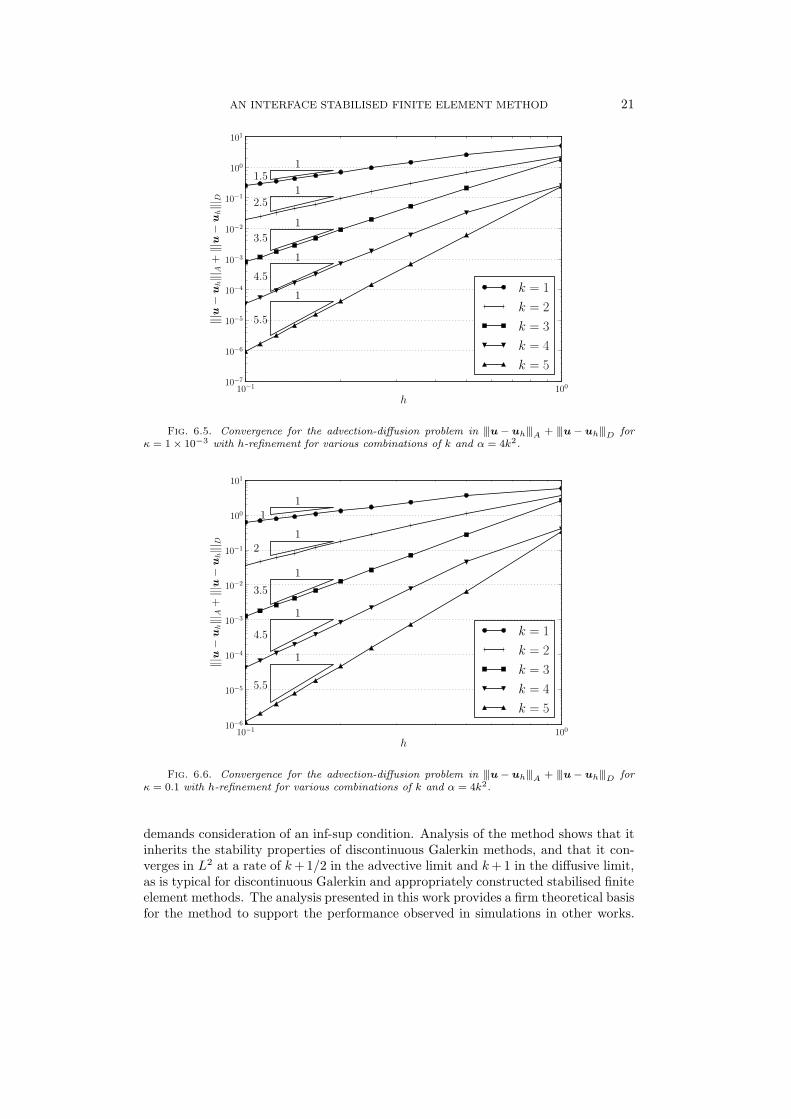
and for various values of κ. The source term f is chosen such that equation (6.2) isthe analytical solution. For all cases, α = 4k2.

The convergence behaviour is examined in terms of |||u− uh|||A + |||u− uh|||D.The computed error for the case κ = 1 × 10−3 is presented in Figure 6.5. For this


10−1

100

h

10−8

10−7

10−6

10−5

10−4

10−3

10−2

10−1

100

101

‖|u−

uh‖|

A

1

1.5

1

2.5

1

3.5

1

4.5

1

5.5

k = 1

k = 2

k = 3

k = 4

k = 5

Fig. 6.1. Convergence for the hyperbolic case with h-refinement for various polynomial orders

in |||·|||A.

10−1

100

h

10−8

10−7

10−6

10−5

10−4

10−3

10−2

10−1

100

‖u−

uh‖ 0

,Ω

1

2

1

3

1

4

1

5

1

6

k = 1

k = 2

k = 3

k = 4

k = 5

Fig. 6.2. Convergence for the elliptic case in L2 with h-refinement for various polynomial

orders and α = 5.

advection dominated problem, the method is observed to converge at the rate k +1/2. For κ = 0.1, the observed convergence response is presented in Figure 6.6. Aconvergence rate of k is observed for the lower order polynomial cases, and the rateappears approach k+1/2 for the higher-order polynomial cases. For κ = 10, which isdiffusion dominated, the observed convergence is presented in Figure 6.7. As expected,a convergence rate of k is observed for the diffusion-dominated case.

20 GARTH N. WELLS

10−1

100

h

10−8

10−7

10−6

10−5

10−4

10−3

10−2

10−1

100

‖u−

uh‖ 0

,Ω

1

2

1

3

1

4

1

5

1

6

k = 1

k = 2

k = 3

k = 4

k = 5


orders and α = 6.

10−1

100

h

10−8

10−7

10−6

10−5

10−4

10−3

10−2

10−1

100

‖u−

uh‖ 0

,Ω

1

2

1

3

1

4

1

5

1

6

k = 1

k = 2

k = 3

k = 4

k = 5


orders and α = 4k2.

7. Conclusions. Stability and error estimates have been developed for an in-terface stabilised finite element method that inherits features of both continuous anddiscontinuous Galerkin methods. The analysis is for the hyperbolic and elliptic limitcases of the advection-diffusion-reaction equation. While the number of global de-grees of freedom on a given mesh for the method is the same as for a continuous finiteelement method, the stabilisation mechanism is the same as that present in upwindeddiscontinuous Galerkin methods. This is borne out in the stability analysis, which


10−1 100

h

10−7

10−6

10−5

10−4

10−3

10−2

10−1

100

101

‖|u−

uh‖|

A+‖|u−

uh‖|

D

1

1.5

1

2.5

1

3.5

1

4.5

1

5.5

k = 1

k = 2

k = 3

k = 4

k = 5

Fig. 6.5. Convergence for the advection-diffusion problem in |||u− uh|||A + |||u− uh|||D for

κ = 1× 10−3 with h-refinement for various combinations of k and α = 4k2.

10−1 100

h

10−6

10−5

10−4

10−3

10−2

10−1

100

101

‖|u−

uh‖|

A+‖|u−

uh‖|

D

1

1

1

2

1

3.5

1

4.5

1

5.5

k = 1

k = 2

k = 3

k = 4

k = 5


κ = 0.1 with h-refinement for various combinations of k and α = 4k2.

demands consideration of an inf-sup condition. Analysis of the method shows that itinherits the stability properties of discontinuous Galerkin methods, and that it con-verges in L2 at a rate of k+1/2 in the advective limit and k+1 in the diffusive limit,as is typical for discontinuous Galerkin and appropriately constructed stabilised finiteelement methods. The analysis presented in this work provides a firm theoretical basisfor the method to support the performance observed in simulations in other works.

22 GARTH N. WELLS

10−1 100

h

10−6

10−5

10−4

10−3

10−2

10−1

100

101

102

‖|u−

uh‖|

A+‖|u−

uh‖|

D

1

1

1

2

1

3

1

4

1

5

k = 1

k = 2

k = 3

k = 4

k = 5


κ = 10 with h-refinement for various combinations of k and α = 4k2.

The analysis results are supported by numerical examples which considered a rangeof polynomial order elements.

Acknowledgement. The author acknowledges the helpful comments on thismanuscript from Robert Jan Labeur and the assistance of Kristian B. Ølgaard inimplementing the features that facilitated the automated generation of the computercode used in Section 6.

References.

[1] T. J. R. Hughes, G. Scovazzi, P. B. Bochev, and A. Buffa. A multiscale discontin-uous Galerkin method with the computational structure of a continuous Galerkinmethod. Computer Methods in Applied Mechanics and Engineering, 195(19-22):2761 – 2787, 2006.

[2] R. J. Labeur and G. N. Wells. A Galerkin interface stabilisation method forthe advection-diffusion and incompressible Navier-Stokes equations. Computer

Methods in Applied Mechanics and Engineering, 196(49–52):4985–5000, 2007.[3] B. Cockburn, B. Dong, J. Guzman, M. Restelli, and R. Sacco. A hybridizable dis-

continuous Galerkin method for steady-state convection-diffusion-reaction prob-lems. SIAM Journal on Scientific Computing, 31(5):3827–3846, 2009.

[4] E. Burman and B. Stamm. Minimal stabilization for discontinuous Galerkin finiteelement methods for hyperbolic problems. Journal of Scientific Computing, 33(2):183–208, 2007.

[5] R. J. Labeur and G. N. Wells. Interface stabilised finite element method formoving domains and free surface flows. Computer Methods in Applied Mechanics

and Engineering, 198(5-8):615 – 630, 2009.[6] A. Buffa, T. J. R. Hughes, and G. Sangalli. Analysis of a multiscale discontinuous

Galerkin method for convection-diffusion problems. SIAM Journal on Numerical

Analysis, 44(4):1420–1440, 2006.[7] A. Ern and J.-L. Guermond. Discontinuous Galerkin methods for Friedrichs’


systems. I. General theory. SIAM Journal on Numerical Analysis, 44(2):753–778, 2006.

[8] D. N. Arnold, F. Brezzi, B. Cockburn, and L. D. Marini. Unified analysis of dis-continuous Galerkin methods for elliptic problems. SIAM Journal on Numerical

Analysis, 39(5):1749–1779, 2002.[9] W. H. Reed and T. R. Hill. Triangular mesh methods for the neutron transport

equation. Technical Report LA-UR-73-479, Los Alamos Scientic Laboratory,1973.

[10] P. Lesaint and P.-A. Raviart. On a finite element method for solving the neutrontransport equation. In Mathematical Aspects of Finite Elements in Partial Dif-

ferential Equations, Publication No. 33, pages 89–123. Math. Res. Center, Univ.of Wisconsin-Madison, Academic Press, New York, 1974.

[11] C. Johnson and J. Pitkaranta. An analysis of the discontinuous Galerkin methodfor a scalar hyperbolic equation. Mathematics of Computation, 46(173):1–26,1986.

[12] M. F. Wheeler. An elliptic collocation-finite element method with interior penal-ties. SIAM Journal on Numerical Analysis, 15(1):152–161, 1978.

[13] D. N. Arnold. An interior penalty finite element method with discontinuouselements. SIAM Journal on Numerical Analysis, 19(4):742–760, 1982.

[14] A. Ern and J.-L. Guermond. Theory and Practice of Finite Elements, volume159 of Applied Mathematical Sciences. Springer-Verlag, New York, 2004.

[15] S. C. Brenner and L. R. Scott. The Mathematical Theory of Finite Element

Methods, volume 15 of Texts in Applied Mathematics. Springer New York, thirdedition, 2008.

[16] L. C. Evans. Partial Differential Equations. American Mathematical Society,Providence, Rhode Island, 1998.

[17] G. N. Wells. Supporting material, 2010. URLhttp://www.dspace.cam.ac.uk/handle/1810/226688.

[18] R. C. Kirby and A. Logg. A compiler for variational forms. ACM Transactions

on Mathematical Software, 32(3):417–444, 2006.[19] K. B. Ølgaard, A. Logg, and G. N. Wells. Automated code generation for dis-

continuous Galerkin methods. SIAM Journal on Scientific Computing, 31(2):849–864, 2008.

[20] K. B. Ølgaard and G. N. Wells. Optimisations for quadrature representations offinite element tensors through automated code generation. ACM Transactions

on Mathematical Software, 37(1):8:1–8:23, 2010.[21] A. Logg and G. N. Wells. DOLFIN: Automated finite element computing. ACM

Transactions on Mathematical Software, 37(2):20:1–20:28, 2010.[22] K. S. Bey and J. T. Oden. hp-Version discontinuous Galerkin methods for hy-

perbolic conservation laws. Computer Methods in Applied Mechanics and Engi-

neering, 133(3–4):259 – 286, 1996.[23] P. Houston, C. Schwab, and E. Suli. Stabilized hp-finite element methods for

first-order hyperbolic problems. SIAM Journal on Numerical Analysis, 37(5):1618–1643, 2000.

http://www.dspace.cam.ac.uk/handle/1810/226688

analysis of an interface stabilised finite element method

Documents