analysis of bright water reservoir sweep improvement...
TRANSCRIPT

ANALYSIS OF BRIGHT WATER RESERVOIR SWEEP IMPROVEMENT AND COMPARISON WITH POLYMER
FLOODING FOR IMPROVED OIL RECOVERY
By:
AKANNI Olatokunbo Olabode
THESIS
Submitted in partial fulfillment of the requirements for the
Degree of Master of Science in Petroleum Engineering
Department of Petroleum and Natural Gas Engineering
New Mexico Institute of Mining and Technology
Socorro New Mexico
December 2010

ABSTRACT
Oil recovery can be improved by injecting fluids into the reservoir via a network
of injection wells to flush oil towards the petroleum production wells. Waterflood is the
most common of this method but associated with it is the problem of early breakthrough
at the production wells and excess water production due to thief zones in the reservoir.
This study examines Bright Water reservoir sweep improvement for waterflooding and
compares with polymer flooding. The slug size of the Bright Water in the higher
permeability reservoir, the position of Bright Water slug in the reservoir and the
permeability contrast of adjacent layers are factors that affect the efficiency of this
reservoir sweep improvement method. Permeability contrast also affects oil recovery for
polymer flooding but not as much as Bright Water. The Bright Water method gives lower
recovery for highly viscous oils but maximum recovery can be obtained with polymer
flood for highly viscous oils by increasing the viscosity of the polymer to obtain
favorable mobility ratio for the displacement process. The cost relation between Bright
Water polymer and normal (HPAM) polymer also plays a role in determining the
profitability of one over the other. Early injection (before 0.5 PV) favors the Bright Water
over polymer flood, but after this the percentage of mobile oil recovered by polymer
flood passes that of Bright Water. The profitability of polymer flood is greater at early
pore volumes of injection (0.5PV – 2.0PV), and vice versa for the Bright Water treatment
method.

ii
ACKNOWLEDGMENT
First and foremost, I would like to use this opportunity to thank my research advisor, Dr.
Randy Seright. Words cannot fully capture how grateful I am to him for giving me the
opportunity to work on this project, his insightful technical knowledge and directions,
and also for his support and encouragement during the course of the research. I would
also like to recognize Dr. Her Yuan Chen and Dr. Thomas Engler for their support and
knowledgeable contributions for this project, special thanks to Dr. Thomas Engler and
Karen Balch for assisting me with unreserved access to the simulation laboratory for the
timely completion of the project. I am grateful to Dr. Robert Lee for support and the
entire staff of the New Mexico Petroleum Recovery Research Center.
I would also like to acknowledge friends and classmates who I have had the privilege of
interacting with during the course of my study, thanks to those who have contributed to
the completion of my study - directly or indirectly. Special thanks to Ronald Adegoke for
providing temporary abode for me in Socorro during my last semester. Most above all, I
will like to express gratitude to my spouse, Olufolake Odufuwa for support and
encouragement during challenging times in the course of this study.
Lastly, I dedicate this work to my parents, Dr. M.S. Akanni and Mrs. B.O. Akanni for
their continued belief in my success and labor of love to offer me the best in life. God
bless you.
iii
TABLE OF CONTENTS
ACKNOWLEDGMENT ........................................................................................................................ ii
TABLE OF CONTENTS ...................................................................................................................... iii
LIST OF TABLES ................................................................................................................................ vi
LIST OF FIGURES ............................................................................................................................. viii
CHAPTER 1 ........................................................................................................................................... 1
INTRODUCTION .................................................................................................................................. 1
1.1 Problem Description ..................................................................................................................... 1
1.2 Research Objectives ...................................................................................................................... 2
CHAPTER 2 ........................................................................................................................................... 4
LITERATURE REVIEW ....................................................................................................................... 4
2.1 Modification of Injection Profile for Waterflooding .................................................................... 4
2.2 Gel Placement to Modify Injection Profiles ................................................................................. 4
2.3 Polymer Flooding .......................................................................................................................... 7
2.4 Bright Water ` ............................................................................................................................... 9
2.4.1 Early Bright Water Development ............................................................................... 9
2.4.2 The nature and Purpose of Bright Water (aka Pop Polymer) ...................................... 9
2.4.3 Reservoir Mechanism of the Bright Water Treatment. ............................................. 10
2.4.4 Technical Field Trials ............................................................................................... 12
2.5 Bright Water versus Polymer Flooding ...................................................................................... 14
CHAPTER 3 ......................................................................................................................................... 17
MATHEMATICAL THEORY AND SIMULATION MODEL DESCRIPTION ............................... 17

iv
3.1 Fractional Flow Equations .......................................................................................................... 17
3.2 Buckley-Leverett Frontal Advance Theory ................................................................................ 20
3.3 Reservoir Model and Conditions ................................................................................................ 28
3.4 Description of Simulation Models .............................................................................................. 29
3.4.1 The Reservoir Base Case .......................................................................................... 30
3.4.2 Polymer Flood Simulation Model ............................................................................. 32
3.4.3 The Bright Water Simulation Model ........................................................................ 33
CHAPTER 4 ......................................................................................................................................... 34
RESULTS AND DISCUSSION .......................................................................................................... 34
4.1 No Crossflow Reservoir Condition. ............................................................................................ 34
4.2 Validation of Simulation Results ................................................................................................ 36
4.3 Bright Water Simulation Results ................................................................................................ 38
4.3.1 Position of Bright Water Slug ................................................................................... 39
4.3.2 Size of Bright Water Slug ......................................................................................... 43
4.4 Bright Water versus Polymer Flood ........................................................................................... 44
4.4.1 Recovery comparison for 1,000 cp Oil ..................................................................... 45
4.4.2 Recovery Comparison for Other Oil Viscosities ....................................................... 48
4.5 Permeability Ratio ...................................................................................................................... 52
4.5.1 Permeability Ratio Effect on Bright Water Recovery ............................................... 52
4.5.2 Permeability Ratio Effect on Polymer Flood Recovery ............................................ 55
4.5.3 Permeability Ratio Effect Comparison of Bright Water and Polymer Flood ............ 56
CHAPTER 5 ......................................................................................................................................... 57
ECONOMICS CONSIDERATIONS ................................................................................................... 57
5.1 Bright Water Polymer Concentration ......................................................................................... 57
5.1.1 Bright Water for 40% of High Permeability Layer ................................................... 58
v
5.1.2 Bright Water for 80% of High Permeability Layer ................................................... 58
5.2 Polymer (HPAM) Concentration ................................................................................................ 59
5.3 Cost Comparison for Bright Water and Polymer Flood ............................................................. 60
5.3.1 Normal Case Comparison ......................................................................................... 60
5.3.2 Optimistic Case Comparison .................................................................................... 63
5.3.3 Extremely Optimistic Case Comparison ................................................................... 65
CHAPTER 6 ......................................................................................................................................... 67
CONCLUSIONS AND RECOMMENDATIONS ............................................................................... 67
6.1 Conclusions ............................................................................................................................. 67
6.2 Recommendations ....................................................................................................................... 68
NOMENCLATURE ............................................................................................................................. 70
REFERENCES ..................................................................................................................................... 73
APPENDIX A: Description of the Basic Reservoir Simulation Model. .............................................. 75
APPENDIX B: Description of the Polymer Model Keywords. ........................................................... 78
vi
LIST OF TABLES
TABLE 3.1: PERTINENT PROPERTIES OF THE RESERVOIR MODELS ............................................ 31
TABLE 4.1: RESULTS OF DIFFERENT SLUG POSITIONS WITH CORRESPONDING RECOVERIES
(IN %) .................................................................................................................................................. 41
TABLE 4.2: RESULTS OF DIFFERENT SLUG SIZES WITH CORRESPONDING RECOVERIES (IN
%) ........................................................................................................................................................ 44
TABLE 4.3: COMPARISON BETWEEN BRIGHT WATER AND POLYMER FLOOD FOR 1,000 CP
OIL ...................................................................................................................................................... 47
TABLE 4.4: COMPARISON BETWEEN BRIGHT WATER AND POLYMER FLOOD FOR 1 CP AND
10 CP OIL ........................................................................................................................................... 49
TABLE 4.5: COMPARISON BETWEEN BRIGHT WATER AND POLYMER FLOOD FOR 100 CP OIL
............................................................................................................................................................. 50
TABLE 4.6: COMPARISON BETWEEN BRIGHT WATER AND POLYMER FLOOD FOR 10,000 CP
OIL ...................................................................................................................................................... 51
TABLE 4.7: PERMEABILITY RATIO COMPARISON FOR BRIGHT WATER (BASE RESERVOIR
CONDITIONS) ................................................................................................................................... 53
TABLE 4.8: PERMEABILITY RATIO COMPARISON FOR BRIGHT WATER (WITH 10% BW) ...... 55
TABLE 4.9: PERMEABILITY RATIO COMPARISON FOR POLYMER FLOOD (10 CP POLYMER) 56
TABLE 5.1: BENEFIT RATIO (I) FOR COST COMPARISON OF 10 CP OIL ....................................... 61
TABLE 5.2: BENEFIT RATIO (I) FOR COST COMPARISON OF 100 CP OIL ..................................... 61
TABLE 5.3: BENEFIT RATIO (I) FOR COST COMPARISON OF 1,000 CP OIL .................................. 61
TABLE 5.4: BENEFIT RATIO (I) FOR COST COMPARISON OF 10,000 CP OIL ................................ 62
TABLE 5.5: BENEFIT RATIO (I) FOR COST COMPARISON OF 10 CP OIL ....................................... 63
TABLE 5.6: BENEFIT RATIO (I) FOR COST COMPARISON OF 100 CP OIL ..................................... 63
TABLE 5.7: BENEFIT RATIO (I) FOR COST COMPARISON OF 1,000 CP OIL .................................. 64
TABLE 5.8: BENEFIT RATIO (I) FOR COST COMPARISON OF 10,000 CP OIL ................................ 64

vii
TABLE 5.9: BENEFIT RATIO (I) FOR COST COMPARISON OF 10 CP OIL ....................................... 65
TABLE 5.10: BENEFIT RATIO (I) FOR COST COMPARISON OF 100 CP OIL ................................... 65
TABLE 5.11: BENEFIT RATIO (I) FOR COST COMPARISON OF 1,000 CP OIL ................................ 65
TABLE 5.12: BENEFIT RATIO (I) FOR COST COMPARISON OF 10,000 CP OIL .............................. 66
viii
LIST OF FIGURES
FIGURE 2.1: INJECTION OF WATER-LIKE GELANT ............................................................................. 5
FIGURE 2.2: INJECTION OF WATER POSTFLUSH PRIOR TO GELATION ......................................... 6
FIGURE 2.3: SHUT-IN DURING GELATION ............................................................................................ 6
FIGURE 2.4: WATER INJECTION AFTER GELATION ........................................................................... 6
FIGURE 2.5: ILLUSTRATION OF WATERFLOOD IN A LAYERED RESERVOIR (WITHOUT
BRIGHT WATER TREATMENT). .................................................................................................... 12
FIGURE 2.6: ILLUSTRATION OF WATER FLOOD IN A LAYERED RESERVOIR WITH THE
BRIGHT WATER TREATMENT. ..................................................................................................... 12
FIGURE 2.7: WATERFLOOD AFTER BRIGHT WATER TREATMENT ............................................... 15
FIGURE 2.8: POLYMER FLOOD FOR A DUAL LAYERED RESERVOIR. .......................................... 15
FIGURE 3.1: TYPICAL FRACTIONAL FLOW CURVE; OIL-WATER SYSTEM. ................................ 19
FIGURE 3.2: FRACTIONAL FLOW VS. WATER SATURATION WITH ITS DERIVATIVE CURVES
............................................................................................................................................................. 24
FIGURE 3.3: EXAMPLE OF A PERFORMANCE PREDICTION CURVE (FROM BL FRONTAL
ADVANCE THEORY) ....................................................................................................................... 27
FIGURE 3.4: SHOWING TANGENT DRAWN TO LOCATE FLOOD FRONTS FOR A POLYMER
FLOOD. ............................................................................................................................................... 28
FIGURE 4.1: BRIGHT WATER TREATMENT FOR A NO CROSSFLOW CASE. ................................ 35
FIGURE 4. 2: GEL PLACEMENT METHOD FOR A NO CROSSFLOW CASE. .................................... 35
FIGURE 4.3: COMPARISON OF THE RECOVERY PLOTS FROM SIMULATOR AND ANALYTICAL
METHOD. ........................................................................................................................................... 37
FIGURE 4.4: COMPARISON OF ANALYTICAL/SIMULATOR RESULTS FOR 1000CP OIL AND
10CP POLYMER INJECTED. ............................................................................................................ 38
FIGURE 4.5: RECOVERY WITH VARIATION IN POSITION OF 40% BRIGHT WATER SLUG IN
THIEF ZONE ...................................................................................................................................... 40

ix
FIGURE 4.6: RECOVERY WITH VARIATION IN POSITION OF 40% BRIGHT WATER SLUG IN
THIEF ZONE UP TO 3 PV INJECTION. .......................................................................................... 41
FIGURE 4.7: SLUG POSITION CLOSE TO PRODUCER ........................................................................ 42
FIGURE 4.8: SLUG POSITION IN THE MIDDLE ................................................................................... 42
FIGURE 4.9: SLUG POSITION CLOSE TO INJECTOR .......................................................................... 43
FIGURE 4.10: RECOVERY WITH VARIATION OF BRIGHT WATER SLUG SIZE IN THIEF ZONE 44
FIGURE 4.11: BRIGHT WATER VERSUS POLYMER FLOOD RECOVERY PLOT FOR 1,000 CP OIL
............................................................................................................................................................. 46
FIGURE 4.12: BRIGHT WATER VS POLYMER FLOOD RECOVERY PLOT FOR 1,000CP OIL
(UNTIL 3 PV INJECTION) ................................................................................................................ 46
FIGURE 4.13: BRIGHT WATER VERSUS POLYMER FLOOD RECOVERY PLOT FOR 1 CP AND 10
CP OIL ................................................................................................................................................ 48
FIGURE 4.14: BRIGHT WATER VERSUS POLYMER FLOOD RECOVERY PLOT FOR 100 CP OIL 49
FIGURE 4.15: BRIGHT WATER VERSUS POLYMER FLOOD RECOVERY PLOT FOR 10,000 CP
OIL ...................................................................................................................................................... 50
FIGURE 4.16: PERMEABILITY RATIO COMPARISON PLOT FOR BRIGHT WATER (BASE
RESERVOIR CONDITIONS) ............................................................................................................ 53
FIGURE 4.17: PERMEABILITY RATIO COMPARISON PLOT FOR BRIGHT WATER (6 GRID
BLOCKS IN VERTICAL AXIS) ........................................................................................................ 54
FIGURE 4.18: PERMEABILITY RATIO COMPARISON PLOT FOR BRIGHT WATER (WITH
10%BW) .............................................................................................................................................. 54
FIGURE 4.19: PERMEABILITY RATIO COMPARISON PLOT FOR POLYMER FLOOD (WITH 10 CP
POLYMER) ......................................................................................................................................... 55
FIGURE 4.20: COMPARISON PLOT FOR PERMEABILITY RATIO EFFECT ON POLYMER FLOOD
AND BRIGHT WATER ..................................................................................................................... 56

1
CHAPTER 1
INTRODUCTION
One of the most common ways employed by the petroleum industry for
improving oil recovery is to flush the oil towards petroleum production wells by injecting
water into the reservoir via a network of injection wells – a process known as waterflood.
A common method also employed is polymer flooding, in which polyacrylamides
or polysaccharides are added to injected water to increase the effectiveness of the water
in displacing oil.
In order for water or polymer flooding to be effective, the injection wells must be
carefully placed. The characteristics of reservoir rock tend to be heterogeneous, or non-
uniform, and the porosity (amount of space between the rock grains) and permeability
(the ability to transmit fluids between the grains) can vary greatly. Formation
heterogeneity affects the performance of most flooding operations, making it a decisive
factor for consideration.
1.1 Problem Description
The injected water can flow fast through thin highly permeable layers of rock,
bypassing much of the oil in the reservoir. These highly permeable layers are known as
‘thief zones’, so-called because they ‘steal’ the injection water. This stolen water then
tends to break through in the production wells, where it causes problems. Every barrel of
water produced must be handled in the oil field’s facilities, treated and either re-injected
2
into the reservoir, or in some cases safely disposed of. All of these can be expensive and
require the use of additional chemicals to process. It takes much time as well as money.
A number of methods are employed by the petroleum industry to tackle this
challenge; the basic concept of these methods is to isolate the thief zones by installing
physical barriers in or near the walls of the injection well boreholes. These range from
inserting devices such as mechanical plugs and patches to injecting polymer gels or
cement. The cements typically go no further than the face of the reservoir rock formation,
and the polymer gels generally don’t penetrate more than about 50 ft (15m).1
Unfortunately, because most thief zones have some degree of contact with the rest
of the reservoir (free crossflow), unless there are extensive vertical permeability barriers,
the injected water can often find its way into the thief zones after getting past the length
of gel penetration.
Since the existing methods do not satisfactorily eradicate this problem, an
industry consortium of some major oil and gas companies was formed and conducted a
multi-company research project known as Bright Water2 to proffer a convincing solution.
1.2 Research Objectives
The major objective of this research work is to analyze the novel ‘Bright Water’
method of reservoir sweep improvement for water flooding and compare the result with
the existing method of direct polymer flooding. The analysis would seek to understand
whether the use of this new sophisticated method is justifiable instead of direct polymer
flooding for improved recovery of oil in place. This main objective can be broken down
into smaller ones as listed below:

3
§ Development of an analytical (mathematical) performance prediction model for
water and polymer flooding processes.
§ Building a water and polymer flooding simulation model for performance
prediction with Schlumberger Eclipse.
§ Comparison of the output from the analytical model and that from the simulation
model.
§ Building a simulation model for the Bright Water treatment process; for
performance prediction with Schlumberger Eclipse.
§ Comparison of the performance of the polymer flooding model with the Bright
Water model under similar reservoir conditions.
§ Variation of pertinent parameters (such as permeability contrast, fluid viscosities
etc) to examine the effects on the performance of both aforementioned methods.
§ Economics analysis on both processes.
4
CHAPTER 2
LITERATURE REVIEW
This chapter examines the existing method of reservoir sweep improvement via
gel placement. A review of direct polymer flooding is also made with a view of giving
the reader a better understanding of the process, keeping the basic research objective in
mind; which is to compare with the Bright Water project.
2.1 Modification of Injection Profile for Waterflooding
As mentioned in the introduction, various methods have been employed to
address the thief zone problem in waterfloods, with the paramount of this being
placement of gels to modify flow profiles.
Near wellbore treatments have been used in attempts to correct waterflood sweep
profile. However in general, the depth of penetration, is typically no more than 15 feet (5
meters)3, and is too small to exert a controlling influence on the reservoir flow unless
extensive barriers to the fluid movement exist orthogonal to the well. Even if vertical
conformance is corrected, areal conformance problems can still be significant.
2.2 Gel Placement to Modify Injection Profiles
The purpose of the gel treatment method is to reduce the flow through fractures or
high permeability zones while diverting injected fluids into the lower permeability
hydrocarbon-bearing layer.4
5
The gel placement method is applied after initial waterflood and premature water
breakthrough in the production well due to injected water flowing through in the high
permeability (thief) zones.
The concept of this method is illustrated in Figure 2.1- 2.4 for a reservoir with a
free crossflow between layers.
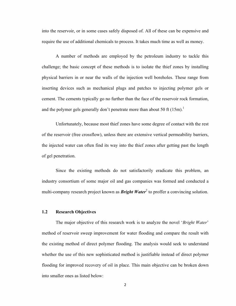
The first step is the injection of a gelant with water-like viscosity, as shown in
Figure 2.1.4 After this step, water is injected to displace the water-like gelant away from
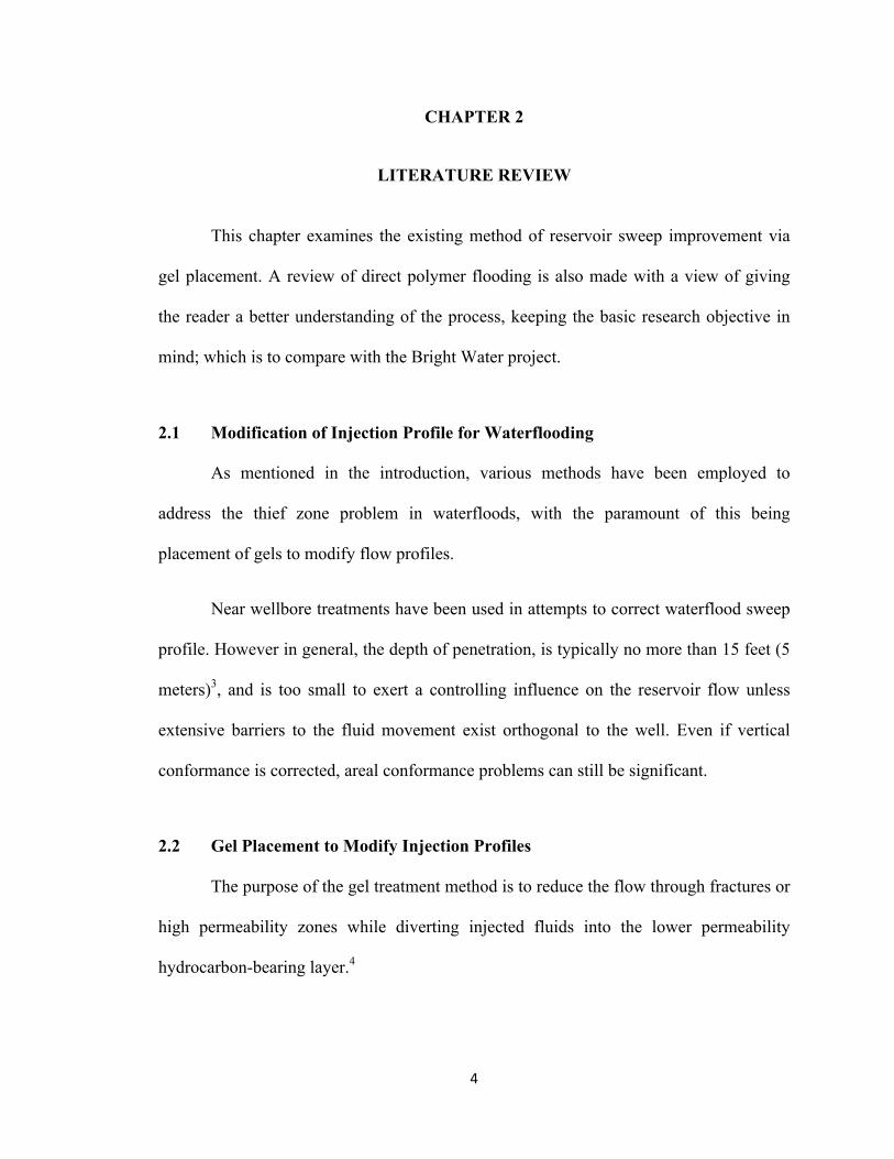
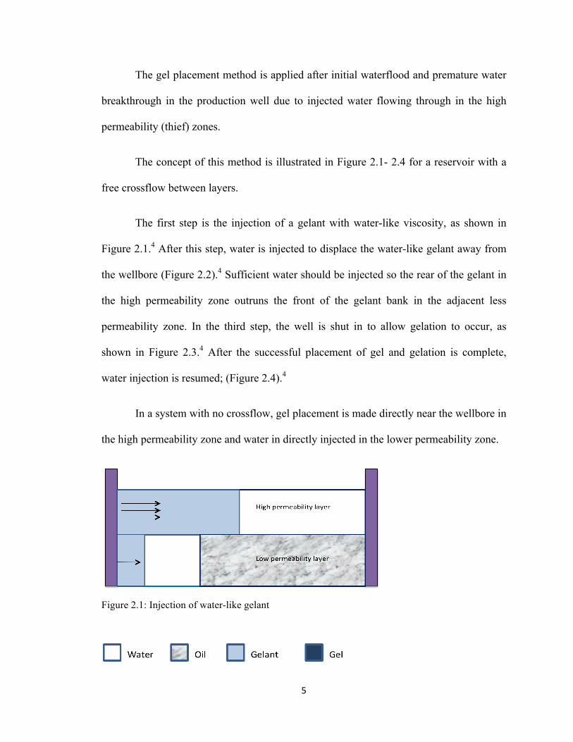
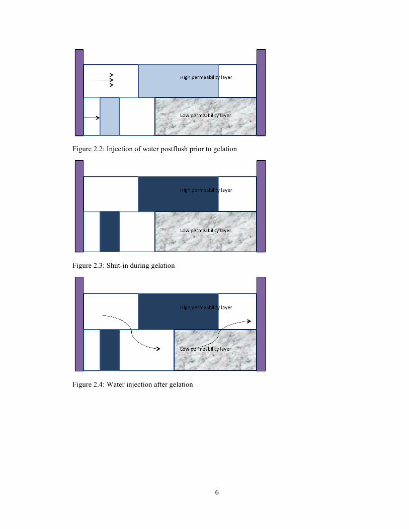
the wellbore (Figure 2.2).4 Sufficient water should be injected so the rear of the gelant in
the high permeability zone outruns the front of the gelant bank in the adjacent less
permeability zone. In the third step, the well is shut in to allow gelation to occur, as
shown in Figure 2.3.4 After the successful placement of gel and gelation is complete,
water injection is resumed; (Figure 2.4).4
In a system with no crossflow, gel placement is made directly near the wellbore in
the high permeability zone and water in directly injected in the lower permeability zone.
Figure 2.1: Injection of water-like gelant
6
Figure 2.2: Injection of water postflush prior to gelation
Figure 2.3: Shut-in during gelation
Figure 2.4: Water injection after gelation
7
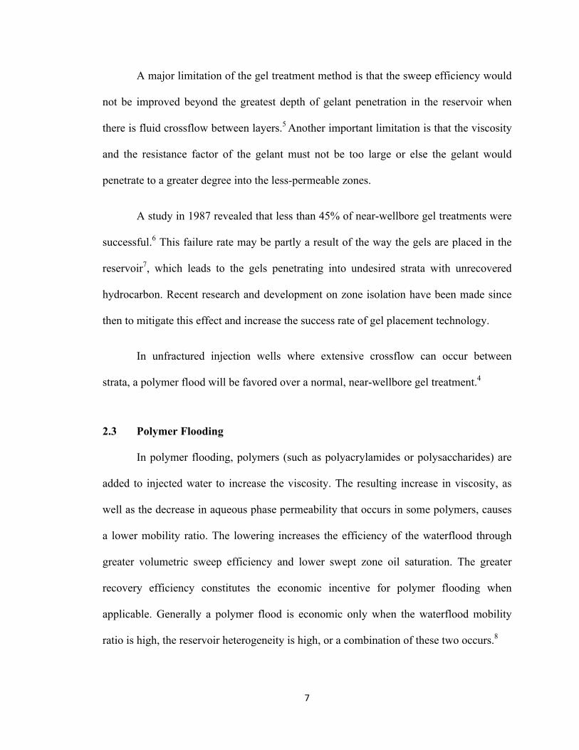
A major limitation of the gel treatment method is that the sweep efficiency would
not be improved beyond the greatest depth of gelant penetration in the reservoir when
there is fluid crossflow between layers.5 Another important limitation is that the viscosity
and the resistance factor of the gelant must not be too large or else the gelant would
penetrate to a greater degree into the less-permeable zones.
A study in 1987 revealed that less than 45% of near-wellbore gel treatments were
successful.6 This failure rate may be partly a result of the way the gels are placed in the
reservoir7, which leads to the gels penetrating into undesired strata with unrecovered
hydrocarbon. Recent research and development on zone isolation have been made since
then to mitigate this effect and increase the success rate of gel placement technology.
In unfractured injection wells where extensive crossflow can occur between
strata, a polymer flood will be favored over a normal, near-wellbore gel treatment.4
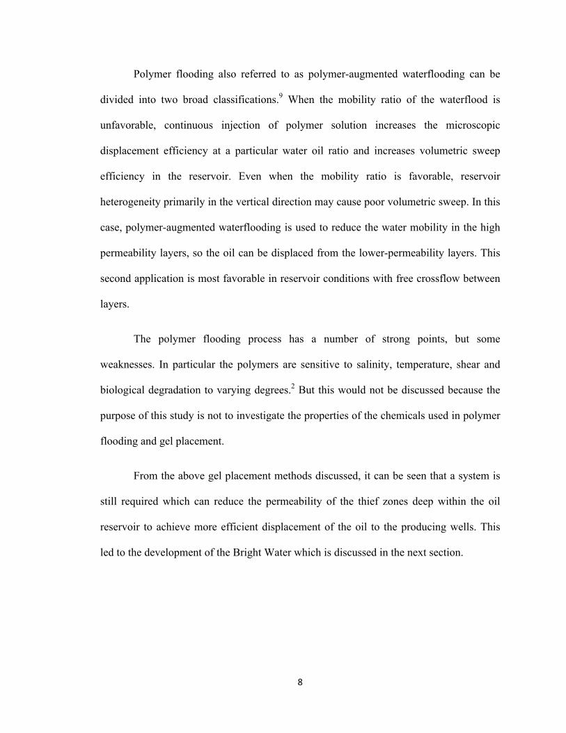
2.3 Polymer Flooding
In polymer flooding, polymers (such as polyacrylamides or polysaccharides) are
added to injected water to increase the viscosity. The resulting increase in viscosity, as
well as the decrease in aqueous phase permeability that occurs in some polymers, causes
a lower mobility ratio. The lowering increases the efficiency of the waterflood through
greater volumetric sweep efficiency and lower swept zone oil saturation. The greater
recovery efficiency constitutes the economic incentive for polymer flooding when
applicable. Generally a polymer flood is economic only when the waterflood mobility
ratio is high, the reservoir heterogeneity is high, or a combination of these two occurs.8
8
Polymer flooding also referred to as polymer-augmented waterflooding can be
divided into two broad classifications.9 When the mobility ratio of the waterflood is
unfavorable, continuous injection of polymer solution increases the microscopic
displacement efficiency at a particular water oil ratio and increases volumetric sweep
efficiency in the reservoir. Even when the mobility ratio is favorable, reservoir
heterogeneity primarily in the vertical direction may cause poor volumetric sweep. In this
case, polymer-augmented waterflooding is used to reduce the water mobility in the high
permeability layers, so the oil can be displaced from the lower-permeability layers. This
second application is most favorable in reservoir conditions with free crossflow between
layers.
The polymer flooding process has a number of strong points, but some
weaknesses. In particular the polymers are sensitive to salinity, temperature, shear and
biological degradation to varying degrees.2 But this would not be discussed because the
purpose of this study is not to investigate the properties of the chemicals used in polymer
flooding and gel placement.
From the above gel placement methods discussed, it can be seen that a system is
still required which can reduce the permeability of the thief zones deep within the oil
reservoir to achieve more efficient displacement of the oil to the producing wells. This
led to the development of the Bright Water which is discussed in the next section.
9
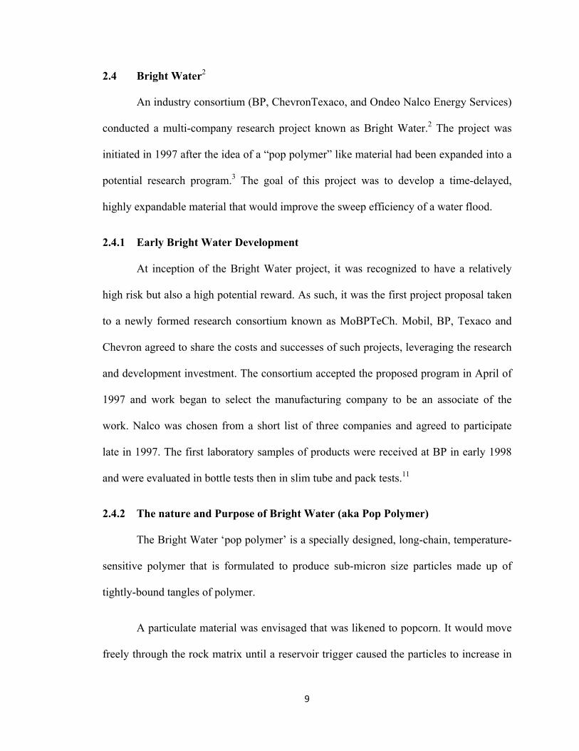
2.4 Bright Water2
An industry consortium (BP, ChevronTexaco, and Ondeo Nalco Energy Services)
conducted a multi-company research project known as Bright Water.2 The project was
initiated in 1997 after the idea of a “pop polymer” like material had been expanded into a
potential research program.3 The goal of this project was to develop a time-delayed,
highly expandable material that would improve the sweep efficiency of a water flood.
2.4.1 Early Bright Water Development
At inception of the Bright Water project, it was recognized to have a relatively
high risk but also a high potential reward. As such, it was the first project proposal taken
to a newly formed research consortium known as MoBPTeCh. Mobil, BP, Texaco and
Chevron agreed to share the costs and successes of such projects, leveraging the research
and development investment. The consortium accepted the proposed program in April of
1997 and work began to select the manufacturing company to be an associate of the
work. Nalco was chosen from a short list of three companies and agreed to participate
late in 1997. The first laboratory samples of products were received at BP in early 1998
and were evaluated in bottle tests then in slim tube and pack tests.11
2.4.2 The nature and Purpose of Bright Water (aka Pop Polymer)
The Bright Water ‘pop polymer’ is a specially designed, long-chain, temperature-
sensitive polymer that is formulated to produce sub-micron size particles made up of
tightly-bound tangles of polymer.
A particulate material was envisaged that was likened to popcorn. It would move
freely through the rock matrix until a reservoir trigger caused the particles to increase in

10
size to block the thief zone pore throats. The thermal front caused by the temperature
differences between the injected water and the reservoir was selected as the most
practical reservoir trigger.3
The product was based on a polymer particle bound in its manufactured, shrunken
form (colloquially referred to as a “kernel” from the analogy of popcorn) by a thermally
sensitive crosslinker, which would break when the particles reached a suitable trigger
temperature. This would allow them to absorb water and increase in size to block pore
throats.
2.4.3 Reservoir Mechanism of the Bright Water Treatment.
For the purpose of this study, the Bright Water is assumed to perform with 100%
accuracy as described by the manufacturers. It will be assumed that the Bright Water has
the same viscosity as water, and that the formulation of the Bright Water molecules can
be adjusted so that the particles will ‘pop’ at different rates and different temperatures.
The product (Bright Water) was engineered to disperse into the injection water
then travel with the water to the problem zone. To avoid loss of particles during
propagation of the treatment to the thermal front, the adsorption and retention of the
particles of the rock pore walls was designed to be minimal until thermally triggered.11
Since the Bright Water is injected with water at the same viscosity, most of it
enters directly into the thief zones and when the molecules get to a certain point in the
reservoir, of the predetermined temperature front change, there is a trigger and the
molecules expand in diameter (“pop” rather like popcorn but a lot slower)10, form
associations and block the rock pores of the high permeability zone.

11
The application of the reagent can be divided into three phases10;
1. Injection, when the particles enter the formation at relatively high velocity. At this
stage the temperature is that of the injection water and relatively low, typically 50
to 120oF. The particles are submicron diameter and inert when injected. This
allows them to enter the formation without causing loss of injectivity.
2. The propagation phase is when the particles, still small and inert, are pushed by
the normal waterflood and move through the pore structure far into the reservoir
at geometrically reducing velocity and increasing temperature gradient between
the injection water and the reservoir temperature.
3. “Popping” when the particles reach temperatures between 120 and 170oF, internal
crosslinks break and the particles absorb water and grow. With time and
temperature, they react with water, expand and become interactive. They can then
block the pore system they are travelling through. Isothermal application is also
possible with the correct reagent grade selection.
After the popping of the polymer and the thief zone has been blocked, water is then
injected into the reservoir to drive the oil in the lower permeability zone towards the
production well.
Figure 2.516 below shows a normal water flood treatment in a layered reservoir and
this is compared to a Bright Water treatment method in Figure 2.6.16 The second figure
shows the reservoir after the Bright Water has been injected and the polymer had
‘popped’ at the right point in the reservoir as designed by the temperature trigger
mechanism.

12
Figure 2.5: Illustration of waterflood in a layered reservoir (without Bright Water treatment).
Figure 2.6: Illustration of water flood in a layered reservoir with the Bright Water treatment.
2.4.4 Technical Field Trials
Between 1999 and 2000, different fields were considered as possibilities for field
trial. It should be noted that a relatively low oil recovery combined with high water cut in
a pattern that has had a significant pore volume of water injected is a good basis for
concluding that a sweep problem (thief zone) exists.2 Eventually the Chevron Petroleum
Indonesia, Minas field was selected because it fit the requisite selection criteria given
below11:

13
§ Available movable oil reserves
§ Early water breakthrough to high water-cut
§ Problem with high permeability contrast, (thief zone at least 5 times un-swept
zone)
§ Porosity of highest perm zone > 17%
§ Permeability in thief zone > 100 mD
§ Minimal reservoir fracturing
§ Temperature 50 C (122 F) to 150 C (302 F)
§ Expected injector-producer transit time > 30 days
§ Injection water salinity under 70,000 ppm
In November 2001, the first of these water flood profile modification treatments was
pumped in the Minas field. The Minas field, located on the island of Sumatra in
Indonesia, has an OOIP of 8.7 billion barrels, is at nearly 50% recovery, and has water-
cuts greater than 97%.
The purpose of this pilot trial was to test the logistics of supply and application, then
provide unequivocal evidence of in-depth blocking of the thief zone. For this purpose the
top sand of the reservoir, where a small amount of attic oil potential was identified, was
isolated and treated.11
The treatment was executed in November 2001 as stated above, and the results
published (Pritchett et al, 2003).3 It was reported that the treatment caused a block in the
reservoir up to 38 meters away from the injection well, and a small amount of

14
incremental oil was recovered11, but the volume of incremental oil attributable to the
Bright Water treatment is uncertain.3
As part of the continued development of this material, a second trial commenced in
late November 2002 on a North Sea (UK) productions platform. The treatment was
successfully placed in mid December, 2002.2 This proved that treatments could be
injected offshore, even on minimum facility platforms and confirmed that the particles
injected easily into 400 mD (0.395µm2) sandstone without loss of injectivity.
Unfortunately the field was sold before the treatment results were observed for this
particular field.11
A first commercial trial was then arranged for the Milne Point field in Alaska. This is
the subject of a paper by Ohms et al (2009).10 BP deployed the particulate sweep
improvement system in seven BP or BP joint venture operated field up to August 2008
with some recorded level of technical success as reported by Frampton et al.11
2.5 Bright Water versus Polymer Flooding
In as much as technical and some commercial success have been reported so far for
this project, the questions still to be answered are:
§ Is the Bright Water treatment always a better method than polymer flooding?
§ Under what conditions will one be preferred to the other (parameters involved)?
§ What are the cost implications of both processes versus recovery potential?
These questions are what this research seeks to answer.

15
Figure 2.7 below shows a case of water flooding after Bright Water treatment for
a reservoir with the high permeability layer already watered out, a critical point to be
examined is how much oil will be recovered for a case with hydraulic contact between
layers (free crossflow). The study will also show the dependency (or otherwise) of the
recovery to the length covered by the popped polymer and amount of pore volumes of
water injected to achieve maximum recovery.
Figure 2.7: Waterflood after Bright Water treatment The main objective will be to compare the output of the Bright Water treated case
with that of the direct polymer flooding – in both cases, with high permeability layer
already watered out - as shown in Figure 2.8.
Figure 2.8: Polymer flood for a dual layered reservoir.

16
The basic tools employed in the course of the research work are analytical and the
results will be cross-examined with numerical simulation; which will then be used for the
comparison of both methods of enhanced oil recovery. More about the mathematical
analysis and simulation will be discussed in next chapter.

17
CHAPTER 3
MATHEMATICAL THEORY AND SIMULATION MODEL DESCRIPTION
This chapter introduces the basics of the Buckley-Leverett frontal advance theory;
it covers fractional flow calculations and the displacement mechanisms described by
frontal advance theory for water and polymer flood performance prediction. The reservoir
model used in the simulation part of the research will also be described in this chapter.
The simulation models to be discussed include those for the waterflood and polymerflood
processes, and also for the Bright Water treatment.
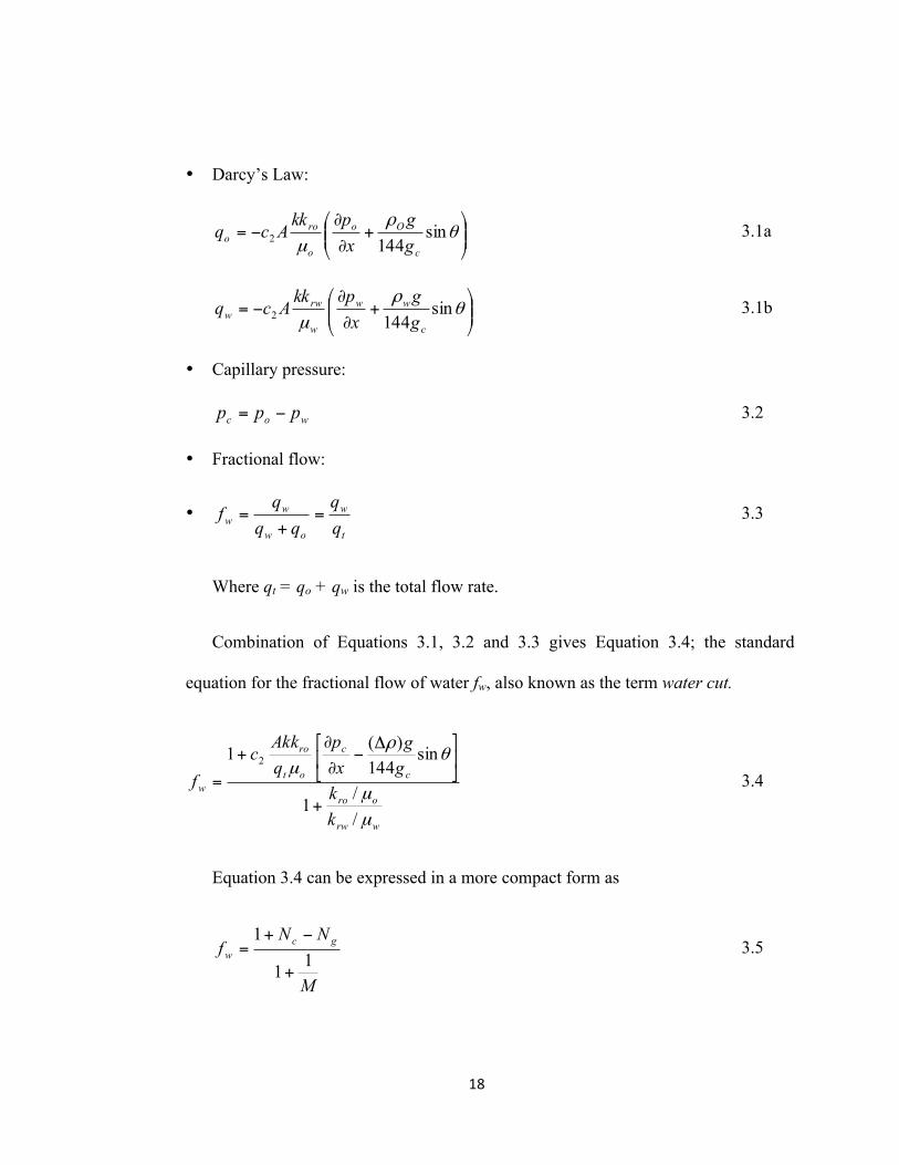
3.1 Fractional Flow Equations
The concept of fractional flow provides the basic understanding of the effects of
the competing driving forces on multiphase flow. The three fundamental forces in a flow
are12:
§ Viscous force (due to fluid viscosity)
§ Capillary force (due to capillary pressure); and
§ Gravity force (due to fluid density or weight)
These three forces are combined together to blend into a single equation known as the
fractional flow equation. Consider a simultaneous oil and water flow (2-phase flow) in
the reservoir. To determine the fraction of each phase flowing, the following equations
are combined12:
18
• Darcy’s Law:
⎟⎟⎠
⎞⎜⎜⎝
⎛+
∂
∂−= θ
ρµ
sin1442
c
Oo
o
roo g
gxpkkAcq 3.1a
⎟⎟⎠
⎞⎜⎜⎝
⎛+
∂
∂−= θ
ρµ
sin1442
c
ww
w
rww g
gxpkkAcq 3.1b
• Capillary pressure:
woc ppp −= 3.2
• Fractional flow:
• t
w
ow
ww q
qqq
qf =+
= 3.3
Where qt = qo + qw is the total flow rate.
Combination of Equations 3.1, 3.2 and 3.3 gives Equation 3.4; the standard
equation for the fractional flow of water fw, also known as the term water cut.
wrw
oro
c
c
ot
ro
w
kk
gg
xp
qAkkc
f
µµ
θρ
µ
//
1
sin144
)(1 2
+
⎥⎦
⎤⎢⎣
⎡ Δ−
∂
∂+
= 3.4
Equation 3.4 can be expressed in a more compact form as
M
NNf gcw 11
1
+
−+= 3.5

19
In the analysis in course of this research, gravity force and capillary pressure
effects are neglected and the fractional flow equation takes a simplified form:
t
ww M
M
M
fλλ
=+
=+
=111
1 3.6
Where λ represents the mobility and λ = kr/µ;
And λt = λo + λw 3.7
As can be seen from Equation 3.6, fractional flow is a function of mobility ratio,
i.e. the mobility ratio governs the fractional flow, rather than the individual phase
mobility.12 A plot of the fractional flow of water against the water saturation values is
known as the fractional flow curve as shown in Figure 3.1 below.
Figure 3.1: Typical fractional flow curve; oil-water system.
0
0.1
0.2
0.3
0.4
0.5
0.6
0.7
0.8
0.9
1
0.0000 0.1000 0.2000 0.3000 0.4000 0.5000 0.6000 0.7000 0.8000
Frac%o
nal fl
ow of w
ater
Water satura%on
20
3.2 Buckley-Leverett Frontal Advance Theory
Essentially, the theory provides an answer to two questions for a water oil
displacement system12:
§ How fast does the flood front move?
§ Where is the flood front located?
The major assumptions of the Buckley-Leverett (BL) theory are:
• Linear flow (1D, constant velocity direction at every point and for all time, and
constant cross-sectional area perpendicular to flow).
• Immiscible fluids (no mass transfer between fluids).
• Incompressible fluids (constant fluid densities).
• Homogeneous medium (constant absolute porosity and permeability)
• Negligible capillary and gravity effects.
• Isothermal flow.
Fractional flow and mass balance are the two major components of the BL frontal
advance theory12:
• Fractional flow (as already given in Equation 3.6)
t
w
wo
ww M
Mfλλ
λλλ
=+
=+
=1
• Mass Balance
0)(
=∂
∂+
∂
∂⎥⎦
⎤⎢⎣
⎡
tS
xS
dSdftu ww
w
wt
φ 3.8

21
Equation 3.8 is a 1D, first order, non-linear, hyperbolic-type partial differential
equation. The dependent variable is Sw ≡ Sw(x,t) while the independent variables are x and
t. It is non-linear in Sw because the coefficient dfw/dSw is a function of the dependent
variable Sw.
The rate of advance of a saturation Sw is obtained by setting the total derivative
dSw equal to zero.12
0=∂
∂+
∂
∂= dt
tSdx
xSdS ww
w 3.9
And then rearranging,
x
w
x
w
S xS
tS
dtdx
w
⎟⎠
⎞⎜⎝
⎛∂
∂⎟⎠
⎞⎜⎝
⎛∂
∂−=⎟
⎠
⎞⎜⎝
⎛ 3.10
Solving Equations 3.8 and 3.10 results in the following two equations:
• Advancing velocity
ww
w
Sw
wt
SS dS
dftudtdxtv ⎟⎟
⎠
⎞⎜⎜⎝
⎛=⎟
⎠
⎞⎜⎝
⎛=
φ)(
)( 3.11
• Advancing location
w
ww
Sw
wiSS dS
dfAtW
txtx ⎟⎟⎠
⎞⎜⎜⎝
⎛+==
φ)(
6146.5)0()( 3.12
Where;
vSw(t) = ‘true or interstitial’ velocity of saturation Sw at time t, ft/d
xSw(t) = location of saturation Sw at time t, ft.

22
xSw(0) = location of saturation Sw at initial time (t = 0), ft
∫ ∫==t t
tti dtuAdtqtW0 0
6146.5/)()( , cumulative water injected at time t, rb
(dfw/dSw)Sw = the derivative of fw-curve at saturation Sw, dimensionless
Note that Wi(t=0) = 0. The other notations can be found in nomenclature before the
appendices.
Eliminating (dfw/dSw)Sw between Equations 3.11 and 3.12 gives a relationship
between distance and velocity,
)()()(
)0()( tvtqtW
txtx Swt
iSwSw +== 3.13
Where qt = Aut/5.6146. The term Wi/qt reflects a ‘time’ scale12
For dimensionless representation, Equation 3.11 can be rearranged as
Sww
w
t
Sw
dSdf
tutv
⎟⎟⎠
⎞⎜⎜⎝
⎛=
φ/)()(
3.14
The left-hand-side term is a dimensionless advancing velocity at a given Sw. This
dimensionless velocity is constant for a given Sw, because the right-hand-side is a
constant for a specified Sw. Similarly, rearranging equation 3.12 gives a dimensionless
advancing distance as
Sww
wiD
Sww
wiSwSw
dSdftW
dSdf
ALW
Lxtx
⎟⎟⎠
⎞⎜⎜⎝
⎛=⎟⎟
⎠
⎞⎜⎜⎝
⎛=
−)(6146.5
)0()(φ
3.15

23
Where;
L = distance between producer and injector, ft.
WiD = Wi/Vp, dimensionless number of pore volumes (PV) of cumulative water injected
Vp = ALϕ/5.6146, pore volume, rb
As previously stated, Figure 3.1 is a typical plot of a fractional flow vs. saturation.
The derivative, δfw/δSw, can be evaluated graphically by constructing tangents to the fw -
Sw curve at a given saturation or numerically if the relative permeabilities, kro(Sw) and
krw(Sw), are available.
For many combinations of fluids and rock properties, the frontal advance solution
is characterized by a saturation discontinuity at the flood front where the water saturation
jumps the flood-front saturation. This discontinuity occurs because the velocities of the
low water saturations are less than the velocity of the flood front saturation and are
overtaken by this saturation.9
The flood-front saturation is found by constructing a tangent to the fractional-flow
curve from the initial water saturation point. From this, the breakthrough point of injected
water can be found and the pore volume is calculated from inverse of the derivative.
After this, pore volume of water injected with the corresponding values of oil recovered
can be estimated as would be shown by the fractional flow curve plot in Figure 3.2.

24
Figure 3.2: Fractional flow vs. Water saturation with its derivative curves 12
To calculate (graphically) the pore volumes injected and oil recovered from a
waterflood process, the procedures listed below are followed12:
i. Compute relative permeability, fractional flow, and derivative curves:
compute and plot relative permeability curves (kr vs. Sw), fractional flow and its
derivative curves (fw and f’w = dfw/dSw vs. Sw).
Note the following:
Water phase: nwwrwrw Skk )( '0= 3.16
Oil phase: nowroro Skk )( '0= 3.17

25
Where; wror
wrww SS
SSS−−
−=1
' 3.18
MMfw +
=1 (As given in Equation 3.6)
Where; no
w
nww
SS
MM)1()('
'0
−=
3.19
oro
wrw
kk
Mµµ//
0
00 =
3.20
For first-derivative of fractional flow:
⎟⎟⎠
⎞⎜⎜⎝
⎛
−−+
−×−=
wor
o
wrw
www
w
w
SSn
SSnff
dSdf
1)1(
3.21
Also note the following two limiting conditions at the end point saturations:
(a) Sw = Swr: S’w = M = fw = f’w = 0, and (b) Sw = 1-Sor: S’w = 1, M→∞, fw = 1, and
f’w = 0.
ii. Identify Breakthrough (BT) Characteristics
a. Estimate Swf at the tangent point (see Figure 3.2)
b. Compute fwf (fw evaluated at Swf) and f’wf (dfw/dSw)
c. Check the set {Swf, fwf, f’wf} by the following criterion
wiwf
wf
Swfw
wwf SS
fdSdff
−=≡'
3.22
If the above criterion is not satisfied, repeat steps a. through c. until the
Equation 3.22 is satisfied. The final converged Swf, fwf, and f’wf are the
breakthrough (BT) parameters SwBT, fwBT, and f’wBT respectively.
26
d. Compute WiDBT (dimensionless number of PV of cumulative water injected at BT)
by WiDBT = 1/f’wBT
iii. Calculation of cumulative PV at different points
Before BT: This is the time between time-0 and just-before BT, Swe = Swi,
fwe = 0, f’we = 0, and WiD = 0.5WiDBT.
Just-Before BT: Swe = Swi, fwe = 0, f’we = 0 and WiD = WiDBT.
At and After BT: A set of of properly spaced Swe values from SwBT to a
value less than (1-Sor), i.e SwBT ≤ Swe < (1-Sor), where SwBT is from above step and
(1-Sor) is the flood-out (maximum allowable) Swe.
From the above steps, the cumulative PV on water injected can be obtained and
then with mass balance, the oil recovered from water injected before, at and after
breakthrough is estimated. From this, the performance prediction plot of mobile oil
recovered versus pore volume of fluid injected can be drawn.
Figure 3.3 gives an example of a performance prediction plot, which would be
seen a lot in the course of this research. From fractional flow analysis (described above),
the values are obtained to plot the mobile oil recovered versus injected PV of water.

27
Figure 3.3: Example of a performance prediction curve (from BL frontal advance theory)
The preceding analysis and figure is for a waterflood case (displacing oil of 10
cp), the procedure is basically the same for a polymerflood case except that there are two
flood-fronts in the fractional flow curve analysis (the water front and the polymer front).
The points for these fronts are obtained by plotting the fractional flow curves of the water
(of 1 cp viscosity) and also that of the polymer’s viscosity on the same plot. A tangent is
then constructed from the origin to locate both shock points.9
An example of this in Figure 3.4 below shows a polymerflood case with polymer
of 100 cp displacing oil of 1,000 cp viscosity. The tangent is drawn as explained and after
the polymer and water flood-fronts are obtained, the PV of fluid injected and mobile oil
recovered can be obtained as calculated for the waterflood case.
0
0.2
0.4
0.6
0.8
1
0 2 4 6 8 10
Mob
ile Oil Re
covered (frac%o
n)
Injected Pore Volume (dimensionless)

28
Figure 3.4: Showing tangent drawn to locate flood fronts for a polymer flood.
The procedures already given so far explain how to develop the performance
prediction model for a single layer reservoir, the model for a free crossflow dual layered
reservoir is developed by Dr. Randy Seright14 of New Mexico’s Petroleum Recovery
Research Center and the spreadsheet for this (http://baervan.nmt.edu/randy/home.html) is
used in the analytical comparison with the simulation models. A no-crossflow reservoir
condition is not considered in this study and the reason is explained in the next chapter.
3.3 Reservoir Model and Conditions
The general conditions of the reservoir model for performance prediction via
analytical method are given below. These conditions will be referred to during the course
of this study and the same conditions will be used in building the simulation model which
the analytical results would be compared with - in order to validate the simulation results.
0
0.1
0.2
0.3
0.4
0.5
0.6
0.7
0.8
0.9
1
0.0000 0.1000 0.2000 0.3000 0.4000 0.5000 0.6000 0.7000 0.8000
Frac%o
nal fl
ow of w
ater
Water satura%on
1cP
100cP
29
• Dual layered reservoir; same thickness of layers and free crossflow between
layers.
• No gravity, incompressible fluid, no capillary pressure.
• Polymer retention balances inaccessible pore volume.
• Permeability ratio between layers: 10:1.
• Swi = 0.3, Sor = 0.3, kro = 0.1, kroo = 1
• krw=krwo[(Sw – Swr)/(1 – Sor – Swr)]nw, nw=2
• krw=kroo[(1- Sor – Sw)/(1 – Sor – Swr)]no, no=2
• Water viscosity: 1 cp. Other fluids (oil and polymer) viscosities are stated
when varied.
3.4 Description of Simulation Models
As stated under research objectives, the analytical results of water and polymer
flood will be compared with the results from the simulator. After this, a model for the
Bright Water treatment will be developed on this premise for the main objective of the
work; which is to compare Bright Water with polymer flood.
The software used for the reservoir simulation is Schlumberger Eclipse 300 and
part of the reservoir characteristics used in this is based on results from Kwame’s13 work
on polymer flood simulation in a heterogeneous idealized reservoir with or without
crossflow.

30
3.4.1 The Reservoir Base Case
The black-oil option is selected for the base model; a general-purpose reservoir
simulator was employed to model the performance predictions. The fully implicit
solution method was used to solve the governing equations for the simulation results
presented in this report. It includes options, which models secondary displacement and
polymer flooding for a variety of reservoir geometries. A set of grid blocks totally 50 x 1
x 2 for the xyz directions were used with each grid block sizes of 2 x 5 x 5 in meters,
respectively. Vertical communication between layers was enabled.
The injector well was located in the center of cells (1, 1, 1) and the producer was
placed in the cell (50, 1, 1) of the grid. The wells were set to perforate through both
layers in the vertical (z) direction with direct contact with the entire thickness of the
formation.
The injector wells were constrained to operate at maximum injection pressure of
78.6 atm and injection rate of 100 cubic meters per day. At the same time, the production
well was set to be constrained at bottomhole pressure of 12 atm and 100 cubic meters per
day. This calculation was made as a result of the block sizes sensitivity analysis
conducted13. Other variables including the initial reservoir conditions and PVT properties
are presented in Table 3.1.
The relative permeabilities were computed using a power law model with an
index of 2 for oil and water relative permeability curves. Water relative permeability
endpoint values of 0.1 and oil relative permeability endpoint of value of 1.0 were used.

31
Table 3.1: Pertinent properties of the reservoir models13
Reservoir thickness, m 10
Reservoir length, m 100
Permeability (k1& k2), D 0.1 & 1.0
Reservoir pressure, atm 78.6
Oil density, kg/m3 0.808264
Oil formation volume factor, rm3/sm3 1
Oil viscosities, cp 1, 10, 102, 103 and104
Oil compressibility, atm-1 0
Oil saturation, fraction 0.7
Oil production rate, m3/day 100
Water density, kg/m3 0.999125
Water compressibility, atm-1 0
Water formation volume factor, rm3/sm3 1
Water viscosity, cp 1
Initial connate water saturation, fraction 0.3
Water injection rate, m3/day 100
Number of grid blocks 50 x 1 x 2
Grid block size, m 2 x 5 x 5
Porosity, % 30
Rock compressibility, atm-1 2.0 E-8

32
The above model characteristics describe the base reservoir model used in this
work, Appendix A gives further details on the model. This base model is modified
appropriately for both the polymer flood and Bright Water cases for comparison. This
model was designed with the higher permeability layer on top of the one with lower
permeability. Tests run show a slight but negligible effect of the relative position of the
layers on oil recovery per pore volume of injected fluid. The recovery when the lower
permeability layer is on top is slightly lower than when it is below the higher
permeability layer.
3.4.2 Polymer Flood Simulation Model
The polymer option is enabled in the Eclipse simulator for polymer flood
simulation. The polymer viscosities of 10, 100, and 1000 cp were used in displacing oil
with viscosities 10, 102, 103 and 104 cp. The polymer was assigned non-Newtonian
properties to simulate and ideal solution closest to the analytical result. The injection and
the production wells were constrained at the same pressures same as that of the
waterflooding cases and also controlled by the injection and production rates as given.
Further details on the specifics of the keywords used in the simulator’s polymer option
are provided in Appendix B.
For comparison of polymer flood performance prediction plot with the analytical
results, the reservoir conditions listed above are used, but for the main comparison with
Bright Water, the fluids saturation in the layers was changed. For this second case of
comparison with Bright Water treatment; the high permeability layer was designed to be
watered out with the lower permeability layer retaining initial fluid saturation, i.e. for the

33
high permeability layer; Sw = 0.7 and So = 0.3; the low permeability layer retains initial
saturation values of Sw = 0.3, So = 0.7.
3.4.3 The Bright Water Simulation Model
The Bright Water was designed with the basic reservoir characteristics described
in the base model, but with some changes as described below:
• The higher permeability layer is watered-out with the lower permeability layer
retaining initial fluid saturations. For the high permeability layer; Sw = 0.7 and So
= 0.3. For the lower permeability layer; Sw = 0.3, So = 0.7.
• The Bright Water slug was set into position (varied for different simulation runs)
by totally blocking the pore holes (0% porosity) of the area predetermined to be
occupied by the bright Water slug. The permeability of the area to be covered is
also set to zero.
• The Bright Water slug was set in the watered out high permeability zone, with no
spillage into the lower permeability zone.
• The above assumes (optimistically) ideal behavior during the injection of the BW
into the reservoir, it assumes all the Bright Water fluid flows into the high
permeability zone blocking the only the desired (thief) zone.
The conditions described for the polymer flood and Bright Water are the base
conditions employed in the simulation for the comparison of both oil recovery methods
explained in the next chapter. Any change made would be stated before the presentation
of results. Oil viscosity of 1,000 cp is predominantly used in the comparison runs with
reason to be explained also in the next chapter.

34
CHAPTER 4
RESULTS AND DISCUSSION
This chapter presents and analyzes the simulation results of the Bright Water
profile modification process and the polymer flood recovery method. Different conditions
of both enhanced oil recovery methods are examined and comparisons are made between
the methods, also under varied conditions.
Before the presentation and analysis of the simulation results, a look is taken at
the no crossflow reservoir condition to establish the reason why simulation analysis is not
needed for the Bright Water treatment of a reservoir with no fluid flow between layers.
Then we also examine the degree of agreeability between the analytical and simulation
results for water and polymer flooding which would serve as the basis of the simulation
results comparison.
4.1 No Crossflow Reservoir Condition.
For a layered reservoir in which there is no crossflow of fluid between the layers,
there is no need to employ the sophisticated method of Bright Water treatment to improve
reservoir sweep efficiency. Since there is no crossflow between layers, once the thief
zone is blocked – at any position in the layer – there is no flow of water injected into this
high permeability layer deeper in the reservoir, implying that cheaper methods of near
wellbore treatment can be employed successfully.
Figure 4.1 shows Bright Water treatment for a reservoir with no crossflow
between layers. Applying Darcy’s law to the conditions shown in the diagram:

35
QA = QB = QC
Since Zone B is totally blocked, kB = 0, therefore QB = 0, which means QA and QC
equals zero and there is no flow in the high permeability layer.
The explanation can be applied to a near wellbore treatment for a no crossflow
condition as shown in Figure 4.2. No matter where the high permeability zone is blocked,
there is no flow in the zone, thus allowing further waterflood to properly sweep the low
permeability layer.
Figure 4.1: Bright Water treatment for a no crossflow case.
Figure 4. 2: Gel placement method for a no crossflow case.
CC
CCC
BB
BBB
AA
AAA
LPkA
LPkA
LPkA
Δ
Δ=
Δ
Δ=
Δ
Δ
***
***
***
µµµ

36
Now that it has been shown there is no need to apply a Bright Water treatment to
a no crossflow layered reservoir, the results and discussion chapter focuses on reservoir
conditions with free crossflow for the analysis and comparison of the Bright Water and
polymer flood improved recovery methods.
4.2 Validation of Simulation Results
The accuracy of the simulation results are examined before proceeding with the
presentation and analysis of results. The recovery plots obtained from the simulation is
compared with the analytical results provided by the mathematical work of Dr. Randy
Seright using fractional flow calculations as explained in the previous chapter.
The base reservoir properties and conditions explained in the previous chapter are
used in the simulation for the Bright Water and polymer flood cases; any change to the
original case is specified when made.
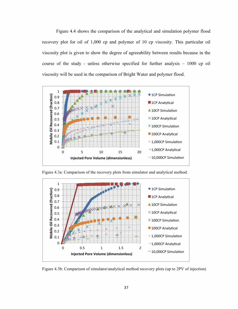
Figures 4.3a and 4.3b gives the waterflood recovery plots showing the
comparison of the analytical and simulation results. It is observed that the results from
the simulator generally gave higher recovery than that of the mathematical work. There is
a close match between oil with viscosities of 1 cp, 1,000 cp and 10,000 cp, but not so
with that of 10 cp and 100 cp; in which the difference considerably widens after injection
of 2 pore volumes (PV) of water. It should be noted volumetric material balance is
maintained; as the results for both the simulator and analytical method converges after
prolonged injection, validating the eventual results of the simulator.
37
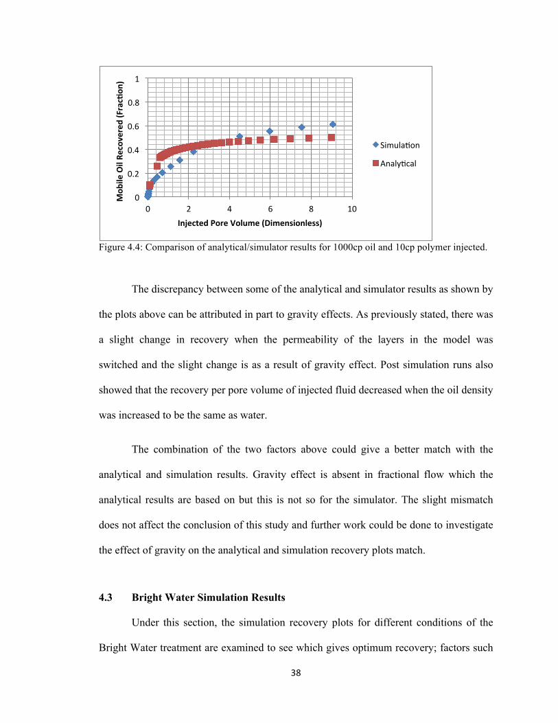
Figure 4.4 shows the comparison of the analytical and simulation polymer flood
recovery plot for oil of 1,000 cp and polymer of 10 cp viscosity. This particular oil
viscosity plot is given to show the degree of agreeability between results because in the
course of the study - unless otherwise specified for further analysis – 1000 cp oil
viscosity will be used in the comparison of Bright Water and polymer flood.
Figure 4.3a: Comparison of the recovery plots from simulator and analytical method.
Figure 4.3b: Comparison of simulator/analytical method recovery plots (up to 2PV of injection)
0 0.1 0.2 0.3 0.4 0.5 0.6 0.7 0.8 0.9 1
0 5 10 15 20
Mob
ile Oil Re
covered (frac%o
n)
Injected Pore Volume (dimensionless)
1CP Simula8on
1CP Analy8cal
10CP Simula8on
10CP Analyi8cal
100CP Simula8on
100CP Analy8cal
1,000CP Simula8on
1,000CP Analy8cal
10,000CP Simula8on
0 0.1 0.2 0.3 0.4 0.5 0.6 0.7 0.8 0.9 1
0 0.5 1 1.5 2
Mob
ile Oil Re
covered (frac%o
n)
Injected Pore Volume (dimensionless)
1CP Simula8on
1CP Analy8cal
10CP Simula8on
10CP Analyi8cal
100CP Simula8on
100CP Analy8cal
1,000CP Simula8on
1,000CP Analy8cal
10,000CP Simula8on
38
Figure 4.4: Comparison of analytical/simulator results for 1000cp oil and 10cp polymer injected.
The discrepancy between some of the analytical and simulator results as shown by
the plots above can be attributed in part to gravity effects. As previously stated, there was
a slight change in recovery when the permeability of the layers in the model was
switched and the slight change is as a result of gravity effect. Post simulation runs also
showed that the recovery per pore volume of injected fluid decreased when the oil density
was increased to be the same as water.
The combination of the two factors above could give a better match with the
analytical and simulation results. Gravity effect is absent in fractional flow which the
analytical results are based on but this is not so for the simulator. The slight mismatch
does not affect the conclusion of this study and further work could be done to investigate
the effect of gravity on the analytical and simulation recovery plots match.
4.3 Bright Water Simulation Results
Under this section, the simulation recovery plots for different conditions of the
Bright Water treatment are examined to see which gives optimum recovery; factors such
0
0.2
0.4
0.6
0.8
1
0 2 4 6 8 10
Mob
ile Oil Re
covered (Frac%on
)
Injected Pore Volume (Dimensionless)
Simula8on
Analy8cal
39
as the position and length of the pop polymer slug in the block thief zone, change in
permeability ratio between layers is later made to see how much this affects the recovery
per pore volume of fluid injected.
4.3.1 Position of Bright Water Slug
The simulation for this case was designed for a dual layered reservoir with
conditions as specified in the previous chapter for a Bright Water case, i.e. with the
higher permeability layer is already watered out; no more mobile oil available in the
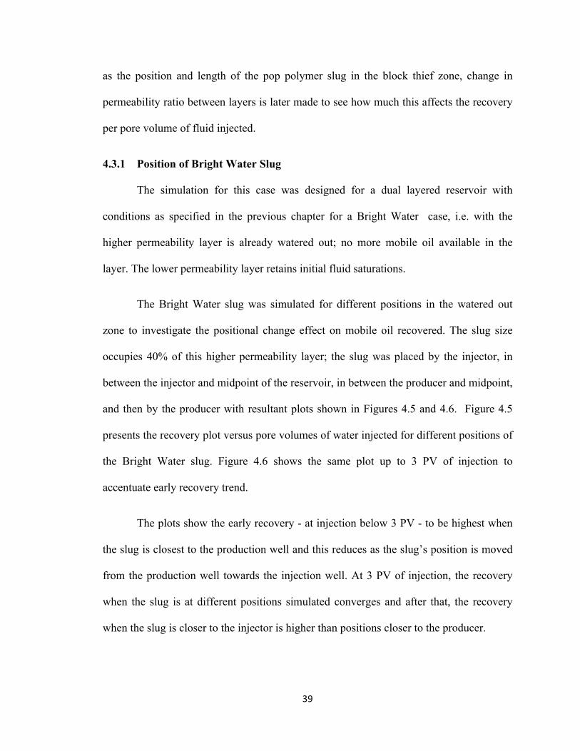
layer. The lower permeability layer retains initial fluid saturations.
The Bright Water slug was simulated for different positions in the watered out
zone to investigate the positional change effect on mobile oil recovered. The slug size
occupies 40% of this higher permeability layer; the slug was placed by the injector, in
between the injector and midpoint of the reservoir, in between the producer and midpoint,
and then by the producer with resultant plots shown in Figures 4.5 and 4.6. Figure 4.5
presents the recovery plot versus pore volumes of water injected for different positions of
the Bright Water slug. Figure 4.6 shows the same plot up to 3 PV of injection to
accentuate early recovery trend.
The plots show the early recovery - at injection below 3 PV - to be highest when
the slug is closest to the production well and this reduces as the slug’s position is moved
from the production well towards the injection well. At 3 PV of injection, the recovery
when the slug is at different positions simulated converges and after that, the recovery
when the slug is closer to the injector is higher than positions closer to the producer.

40
Table 4.1 gives the recovery values at different injection PV, for varying positions
of the Bright Water slug in the high permeability zone.
The table further shows the trend of the oil recovery with different positions of the
Bright Water slug. As stated before, the general trend shows that for injection below 3
PV there is higher recovery when the position of the slug is closer to the production well,
after that; at increased injection the recovery is higher when the position of the slug is
closer to the injection well. The 3 PV crossover point is concluded to be coincidental
since there was no reason determined for that specific pore volumes of injection.
Figure 4.5: Recovery with variation in position of 40% Bright Water slug in thief zone
0
0.2
0.4
0.6
0.8
1
0 5 10 15 20
Mob
ile Oil Re
covered (Frac%on
)
Injected Pore Volumes (Dimensionless)
From_Inj
Btw_Inj_Mid
Mid_Point
Btw_Mid_Prod
From_Prod
41
Figure 4.6: Recovery with variation in position of 40% Bright Water slug in thief zone up to 3 PV injection.
Table 4.1: Results of different slug positions with corresponding recoveries (in %)
Position of Slug From
Injector
Injector -
Midpoint
Midpoint Midpoint -
Producer
From
Producer
Recovery(%) at 0.5 PV 0.5 6.1 10.5 14.7 20.4
Recovery(%) at 1 PV 3.6 15.8 19.7 21.9 25.2
Recovery(%) at 2 PV 18.1 26.7 27.6 28.9 30.3
Recovery(%) at 3 PV 24.2 31.9 33.5 33.9 33.2
Recovery(%) at 5 PV 34.5 41.0 40.4 40.1 37.1
Recovery(%) at 10 PV 48.4 53.5 51.8 49.8 43.9
Recovery(%) at 15 PV 56.7 61.6 58.9 55.5 48.0
0
0.2
0.4
0.6
0.8
1
0 0.5 1 1.5 2 2.5 3
Mob
ile Oil Re
covered (Frac%on
)
Injected Pore Volumes (Dimensionless)
From_Inj
Btw_Inj_Mid
Mid_Point
Btw_Mid_Prod
From_Prod
42
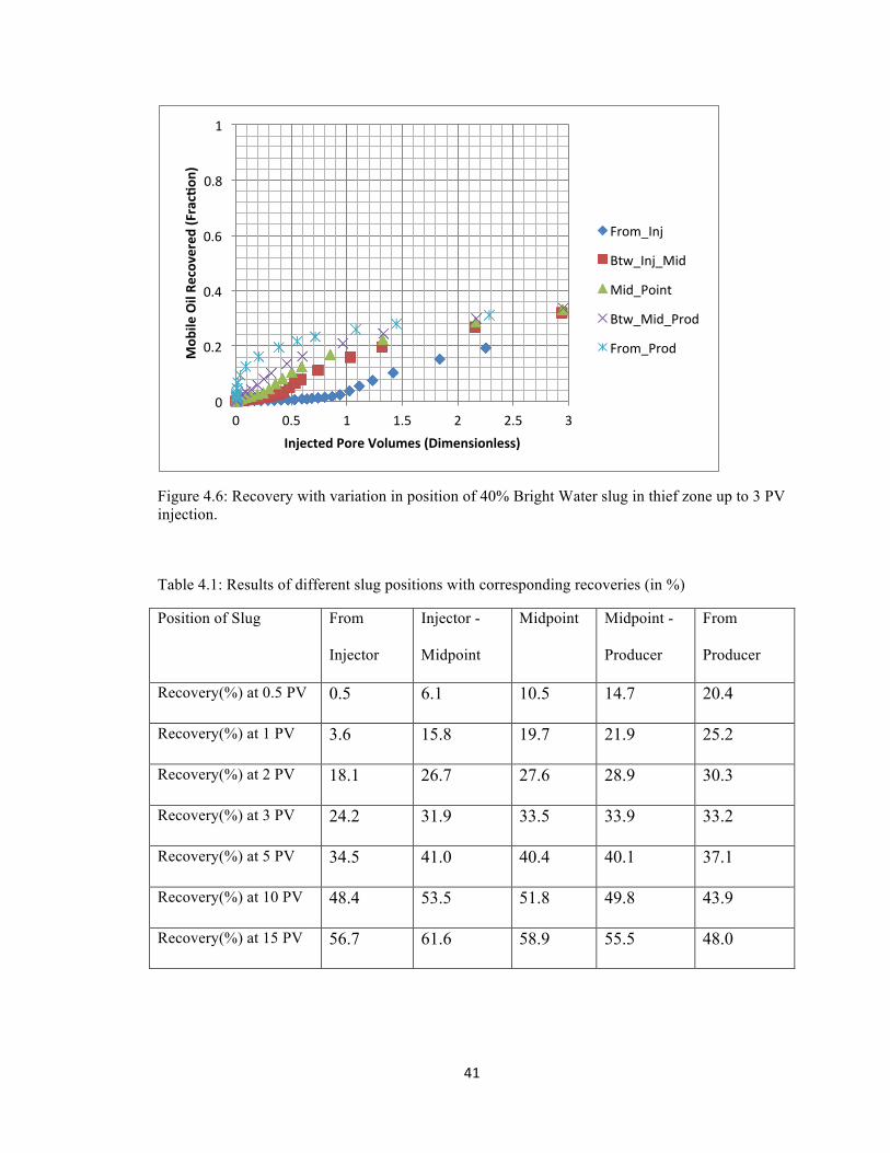
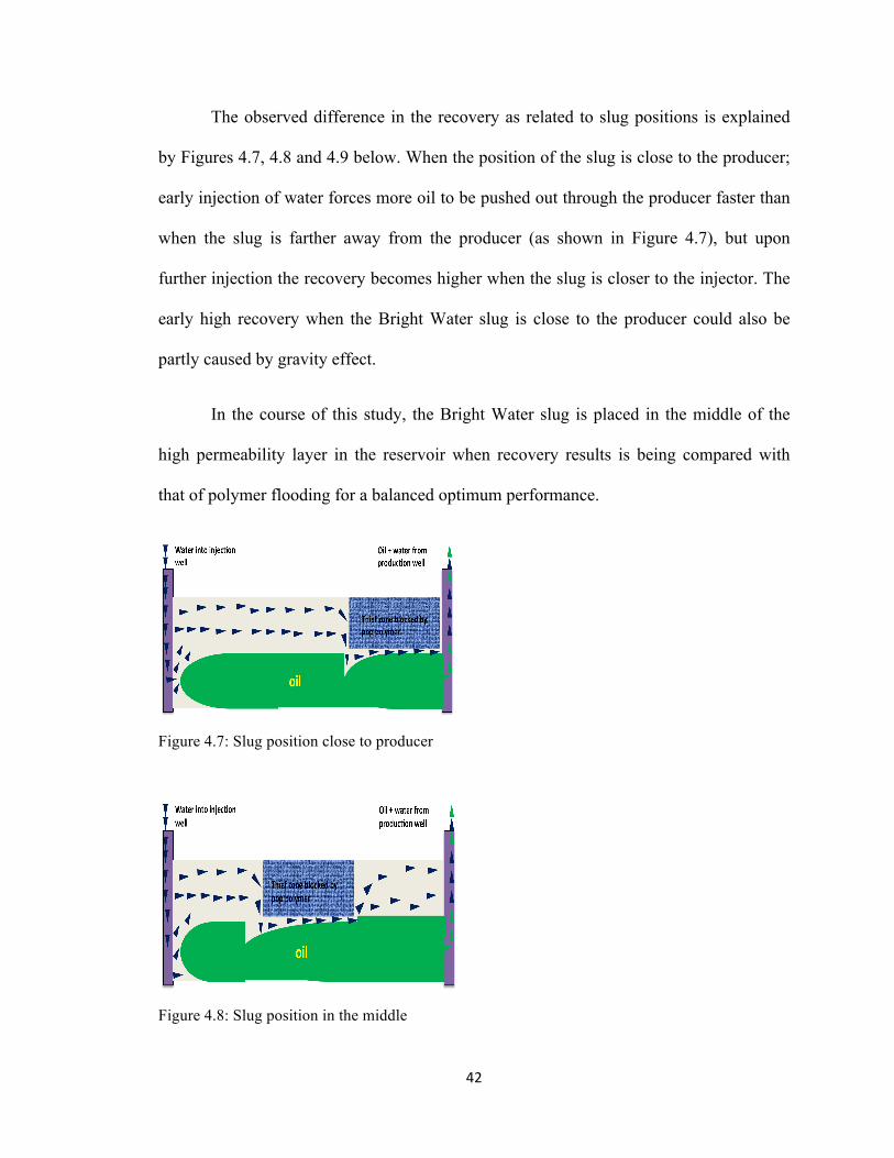
The observed difference in the recovery as related to slug positions is explained
by Figures 4.7, 4.8 and 4.9 below. When the position of the slug is close to the producer;
early injection of water forces more oil to be pushed out through the producer faster than
when the slug is farther away from the producer (as shown in Figure 4.7), but upon
further injection the recovery becomes higher when the slug is closer to the injector. The
early high recovery when the Bright Water slug is close to the producer could also be
partly caused by gravity effect.
In the course of this study, the Bright Water slug is placed in the middle of the
high permeability layer in the reservoir when recovery results is being compared with
that of polymer flooding for a balanced optimum performance.
Figure 4.7: Slug position close to producer
Figure 4.8: Slug position in the middle
43
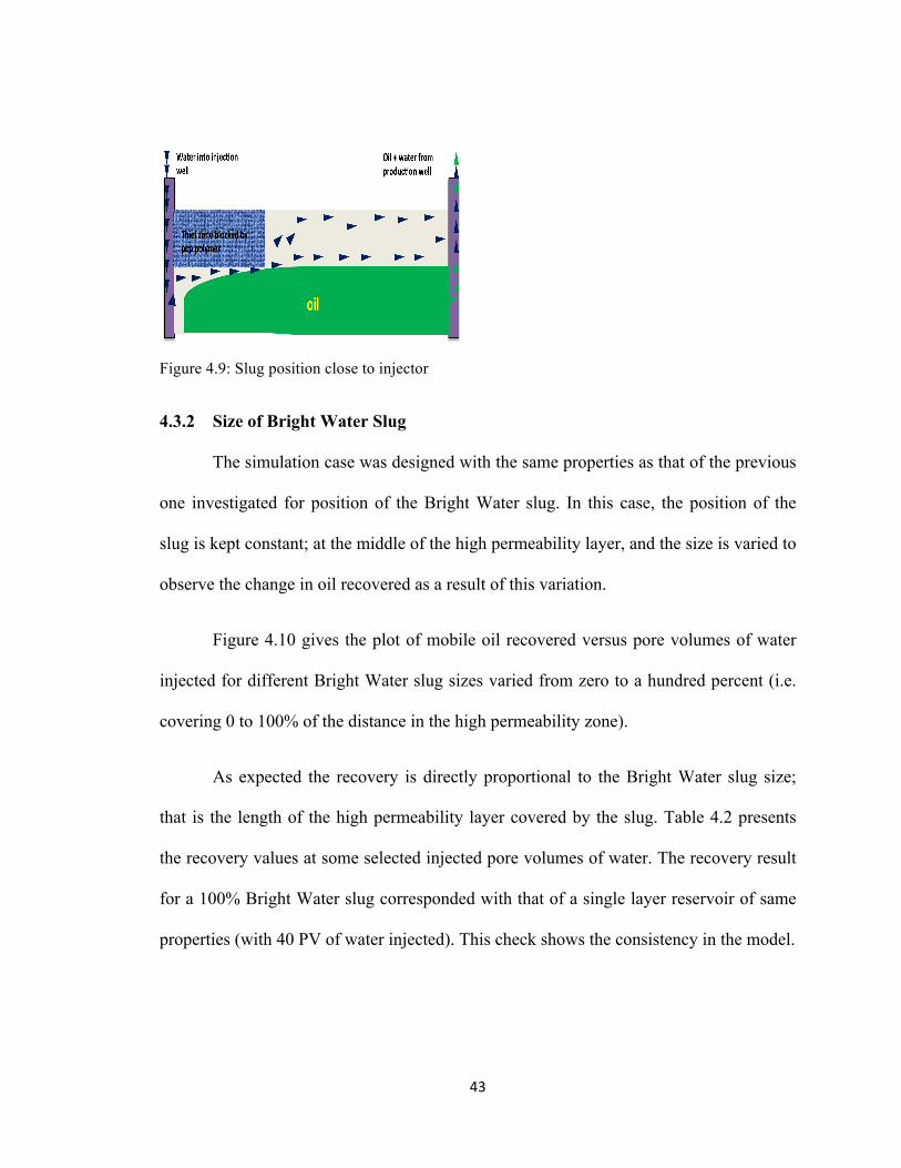
Figure 4.9: Slug position close to injector
4.3.2 Size of Bright Water Slug
The simulation case was designed with the same properties as that of the previous
one investigated for position of the Bright Water slug. In this case, the position of the
slug is kept constant; at the middle of the high permeability layer, and the size is varied to
observe the change in oil recovered as a result of this variation.
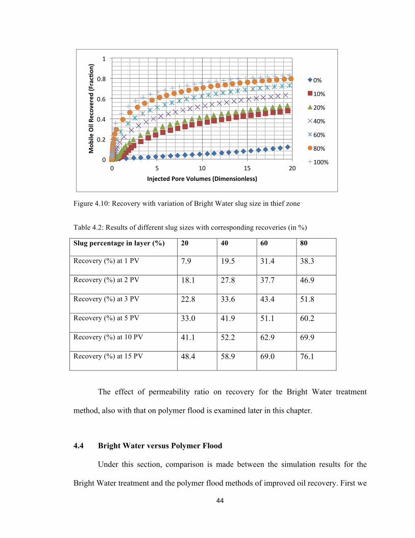
Figure 4.10 gives the plot of mobile oil recovered versus pore volumes of water
injected for different Bright Water slug sizes varied from zero to a hundred percent (i.e.
covering 0 to 100% of the distance in the high permeability zone).
As expected the recovery is directly proportional to the Bright Water slug size;
that is the length of the high permeability layer covered by the slug. Table 4.2 presents
the recovery values at some selected injected pore volumes of water. The recovery result
for a 100% Bright Water slug corresponded with that of a single layer reservoir of same
properties (with 40 PV of water injected). This check shows the consistency in the model.
44
Figure 4.10: Recovery with variation of Bright Water slug size in thief zone
Table 4.2: Results of different slug sizes with corresponding recoveries (in %) Slug percentage in layer (%) 20 40 60 80
Recovery (%) at 1 PV 7.9 19.5 31.4 38.3
Recovery (%) at 2 PV 18.1 27.8 37.7 46.9
Recovery (%) at 3 PV 22.8 33.6 43.4 51.8
Recovery (%) at 5 PV 33.0 41.9 51.1 60.2
Recovery (%) at 10 PV 41.1 52.2 62.9 69.9
Recovery (%) at 15 PV 48.4 58.9 69.0 76.1
The effect of permeability ratio on recovery for the Bright Water treatment
method, also with that on polymer flood is examined later in this chapter.
4.4 Bright Water versus Polymer Flood
Under this section, comparison is made between the simulation results for the
Bright Water treatment and the polymer flood methods of improved oil recovery. First we
0
0.2
0.4
0.6
0.8
1
0 5 10 15 20
Mob
ile Oil Re
covered (Frac%on
)
Injected Pore Volumes (Dimensionless)
0%
10%
20%
40%
60%
80%
100%

45
examine the recovery plots for oil of 1,000 cp viscosity for both methods and then the
plots for oil with viscosities of 1 cp, 10 cp, 100 cp and 10,000 cp are analyzed to see how
the outputs vary with different oil thicknesses.
The base reservoir conditions given in the previous chapter were used in the
simulation for both recovery methods, the recovery plot for the 1,000 cp oil - the default
oil viscosity in the base case - is analyzed first in the next subsection before looking at
the plot for the other listed oil viscosities. In the Bright Water plots, the Bright Water
volume injected before the waterflood is taken note of and included in the PV of fluid
injected.
4.4.1 Recovery comparison for 1,000 cp Oil
Figure 4.11 below shows the Bright Water - polymer flood comparison plot of
mobile oil recovered versus pore volumes of water/polymer injected for oil with 1,000 cp
viscosity. Figure 4.12 gives a closer look at the recovery comparison plot up to 3 PV on
injected fluid, and Table 4.3 presents the recovery values at different pore volumes of
both methods for quick look numerical comparison.
The Figures (4.11 and 4.12) show four curves on a plot; two each for the Bright
Water and the polymer flood simulated recovery processes. The notation PF_10cp
indicates a polymer flood of 10 cp viscosity while PF_100cp indicates a polymerflood of
100 cp viscosity for the 1,000 cp oil. The notation BW_40% indicates a Bright Water
treatment with the Bright Water slug occupying 40% of the watered out higher
permeability layer and BW_80% implies that 80% of the higher permeability layer is

46
covered by the Bright Water slug. The same notation is also used in the results given in
Table 4.3.
Figure 4.11: Bright Water versus polymer flood recovery plot for 1,000 cp oil
Figure 4.12: Bright Water vs polymer flood recovery plot for 1,000cp oil (until 3 PV injection)
0
0.2
0.4
0.6
0.8
1
0 5 10 15 20
Mob
ile Oil Re
covered (Frac%on
)
Injected Pore Volumes (Dimensionless)
PF_10cp
PF_100cp
BW_80%
BW_40%
0
0.2
0.4
0.6
0.8
1
0 0.5 1 1.5 2 2.5 3
Mob
ile Oil Re
covered (Frac%on
)
Injected Pore Volumes (Dimensionless)
PF_10cp
PF_100cp
BW_80%
BW_40%

47
Table 4.3: Comparison between Bright Water and polymer flood for 1,000 cp Oil
BW_40% PF_10 BW_80% PF_100
Recovery (%) at 1 PV 15.1 2.5 29.3 31.6
Recovery (%) at 2 PV 24.5 9.6 41.5 62.5
Recovery (%) at 3 PV 31.6 16.4 46.4 76.1
Recovery (%) at 5 PV 41.5 28.9 55.9 86.8
Recovery (%) at 10 PV 51.9 49.9 67.8 94.1
Recovery (%) at 15 PV 58.8 64.2 73.9 97.4
From the plots and table above, the Bright Water banks of 40% and 80% give a
higher recovery when compared to polymer flood of 10 cp for less than 10 PV. At 10 PV
injection, the 40% BW and 10 cp polymer both give approximately 50% recovery. After
10 PV, the recovery of 10 cp polymerflood passes that of the 40% Bright Water. The
lower recovery of the polymer flood at early injection (before 0.5 PV) can be attributed to
the time required for the polymer to displace the water resident in the watered-out higher
permeability zone. After this point the recovery picks up as more polymer is injected.
The recovery is highest for the 100 cp polymer. At 1 PV of injection, the recovery
for the 100 cp polymer is 31.6% and the next highest is that of 80% BW, which is 29.3%.
After this – 1 PV injection – the recovery from the 100 cp polymer increases at a much
higher rate than the compared method, almost doubling that of the 80% BW at 3 PV of
injection.

48
4.4.2 Recovery Comparison for Other Oil Viscosities
The recovery plots and results for other oil viscosities comparing the Bright Water
output to that of the polymer flood are given in the following figures and tables. The
basic reservoir conditions given earlier were used in the simulation cases for both
recovery methods with the oil viscosities examined.
Figure 4.13 and Table 4.4 presents the recovery comparison plot and table for 1
cp and 10 cp oil, Figure 4.14 and Table 4.5 gives that for 100 cp oil, and the comparison
results for 10,000 cp oil are presented in Figure 4.15 and Table 4.6.
Figure 4.13: Bright Water versus polymer flood recovery plot for 1 cp and 10 cp oil
0
0.2
0.4
0.6
0.8
1
0 1 2 3 4
Mob
ile Oil Re
covered (Frac%on
)
Injected Pore Volumes (Dimensionless)
1cpOil_40%BW
1cpOil_1cpWater
10cpOil_40%BW
10cpOil_10cpPolymer

49
Table 4.4: Comparison between Bright Water and polymer flood for 1 cp and 10 cp oil 1cpOil
BW_40%
1cpOil
1cpWater
10cpOil
BW_40%
10cpOil
10cpWater
Recovery (%) at 0.5 PV 95.9 85.4 67.9 41.7
Recovery (%) at 1 PV 99.9 93.9 84 86.1
Recovery (%) at 2 PV 99.9 98.8 92.9 97.5
Recovery (%) at 3 PV 99.9 99.6 95.5 98.9
Recovery (%) at 3.5 PV 99.9 99.9
97.6 99.5
Figure 4.14: Bright Water versus polymer flood recovery plot for 100 cp oil
0
0.2
0.4
0.6
0.8
1
0 2 4 6 8 10
Mob
ile Oil Re
covered (Frac%on
)
Injected Pore Volumes
40%BW
80%BW
10cpPolymer
100cpPolymer
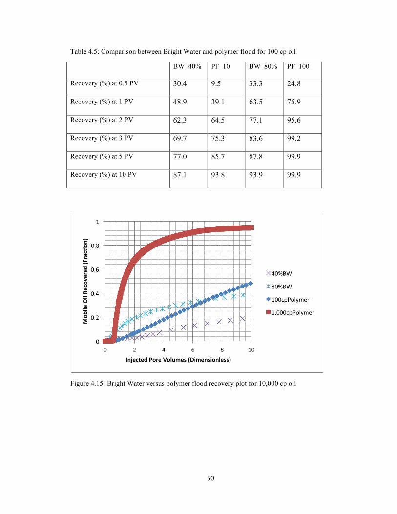
50
Table 4.5: Comparison between Bright Water and polymer flood for 100 cp oil BW_40% PF_10 BW_80% PF_100
Recovery (%) at 0.5 PV 30.4 9.5 33.3 24.8
Recovery (%) at 1 PV 48.9 39.1 63.5 75.9
Recovery (%) at 2 PV 62.3 64.5 77.1 95.6
Recovery (%) at 3 PV 69.7 75.3 83.6 99.2
Recovery (%) at 5 PV 77.0 85.7 87.8 99.9
Recovery (%) at 10 PV 87.1 93.8 93.9 99.9
Figure 4.15: Bright Water versus polymer flood recovery plot for 10,000 cp oil
0
0.2
0.4
0.6
0.8
1
0 2 4 6 8 10
Mob
ile Oil Re
covered (Frac%on
)
Injected Pore Volumes (Dimensionless)
40%BW
80%BW
100cpPolymer
1,000cpPolymer
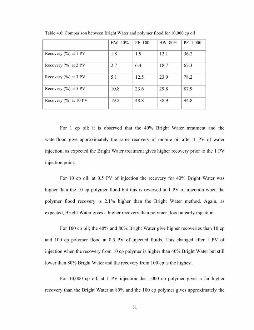
51
Table 4.6: Comparison between Bright Water and polymer flood for 10,000 cp oil BW_40% PF_100 BW_80% PF_1,000
Recovery (%) at 1 PV 1.8 1.9 12.1 36.2
Recovery (%) at 2 PV 2.7 6.4 18.7 67.3
Recovery (%) at 3 PV 5.1 12.5 23.9 78.2
Recovery (%) at 5 PV 10.8 23.6 29.8 87.9
Recovery (%) at 10 PV 19.2 48.8 38.9 94.8
For 1 cp oil; it is observed that the 40% Bright Water treatment and the
waterflood give approximately the same recovery of mobile oil after 1 PV of water
injection, as expected the Bright Water treatment gives higher recovery prior to the 1 PV
injection point.
For 10 cp oil; at 0.5 PV of injection the recovery for 40% Bright Water was
higher than the 10 cp polymer flood but this is reversed at 1 PV of injection when the
polymer flood recovery is 2.1% higher than the Bright Water method. Again, as
expected, Bright Water gives a higher recovery than polymer flood at early injection.
For 100 cp oil; the 40% and 80% Bright Water give higher recoveries than 10 cp
and 100 cp polymer flood at 0.5 PV of injected fluids. This changed after 1 PV of
injection when the recovery from 10 cp polymer is higher than 40% Bright Water but still
lower than 80% Bright Water and the recovery from 100 cp is the highest.
For 10,000 cp oil; at 1 PV injection the 1,000 cp polymer gives a far higher
recovery than the Bright Water at 80% and the 100 cp polymer gives approximately the
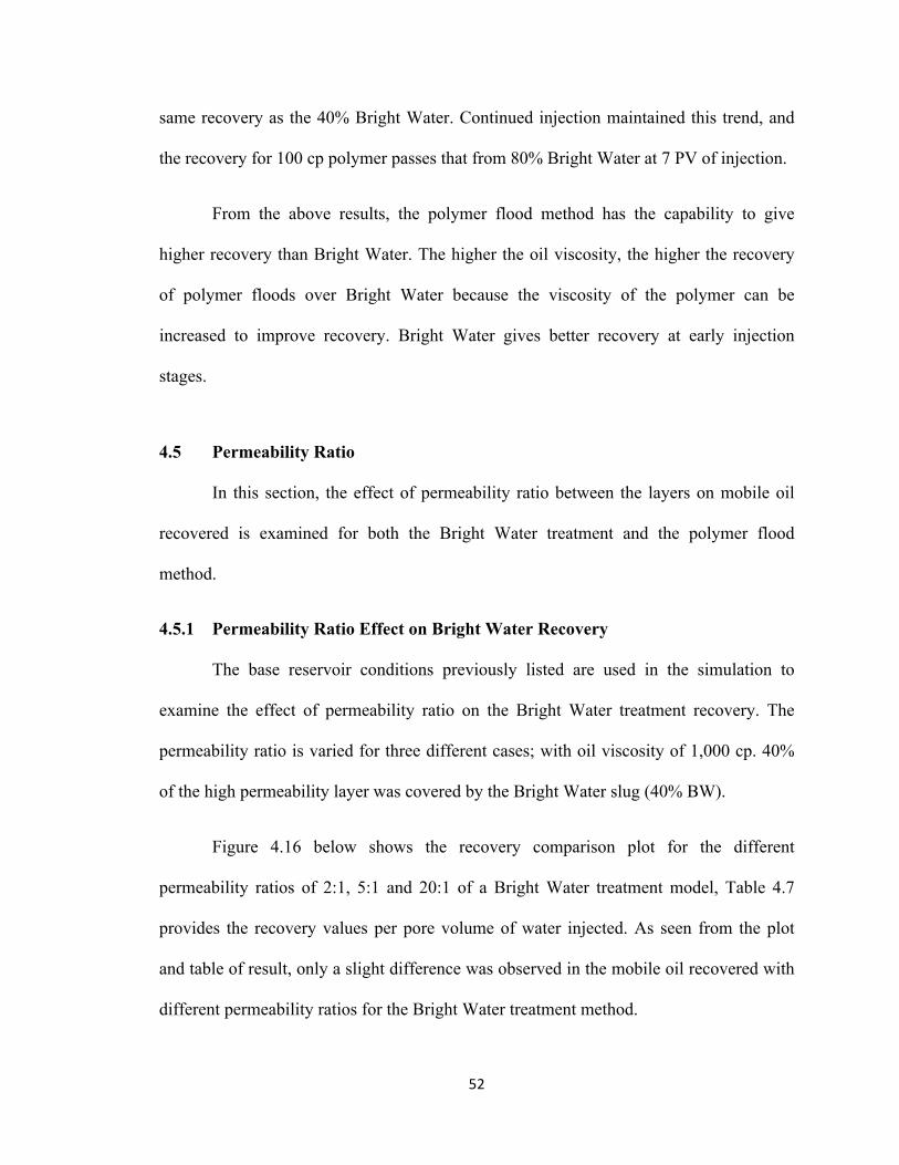
52
same recovery as the 40% Bright Water. Continued injection maintained this trend, and
the recovery for 100 cp polymer passes that from 80% Bright Water at 7 PV of injection.
From the above results, the polymer flood method has the capability to give
higher recovery than Bright Water. The higher the oil viscosity, the higher the recovery
of polymer floods over Bright Water because the viscosity of the polymer can be
increased to improve recovery. Bright Water gives better recovery at early injection
stages.
4.5 Permeability Ratio
In this section, the effect of permeability ratio between the layers on mobile oil
recovered is examined for both the Bright Water treatment and the polymer flood
method.
4.5.1 Permeability Ratio Effect on Bright Water Recovery
The base reservoir conditions previously listed are used in the simulation to
examine the effect of permeability ratio on the Bright Water treatment recovery. The
permeability ratio is varied for three different cases; with oil viscosity of 1,000 cp. 40%
of the high permeability layer was covered by the Bright Water slug (40% BW).
Figure 4.16 below shows the recovery comparison plot for the different
permeability ratios of 2:1, 5:1 and 20:1 of a Bright Water treatment model, Table 4.7
provides the recovery values per pore volume of water injected. As seen from the plot
and table of result, only a slight difference was observed in the mobile oil recovered with
different permeability ratios for the Bright Water treatment method.

53
Figure 4.16: Permeability ratio comparison plot for Bright Water (Base reservoir conditions)
Table 4.7: Permeability ratio comparison for Bright Water (Base reservoir conditions) Permeability Ratio 2:1 5:1 20:1
Recovery (%) at 1 PV 20.9 18.6 17.5
Recovery (%) at 4 PV 40.0 38.9 37.1
Recovery (%) at 8 PV 52.7 50.0 48.5
In order to accentuate the effect of the permeability ratio on recovery for Bright
Water, the simulation base case was modified from 2 grid blocks in the vertical direction
to 6 grid blocks; other conditions were kept the same. Fig. 4.17 presents the result of this
grid block modification.
The plot shows the recovery of the model with 6 grid blocks in the vertical
direction and the base one with 2 grid blocks in the vertical direction to be the same and
the refining of grid blocks had no effect on the result. This confirms the permeability
ratio only has a slight effect on the recovery for the 40% Bright Water.
0
0.2
0.4
0.6
0.8
1
0 2 4 6 8 10 Mob
ile Oil Re
covered (Frac%on
)
Injected Pore Volumes (Dimensionless)
2_1
5_1
20_1
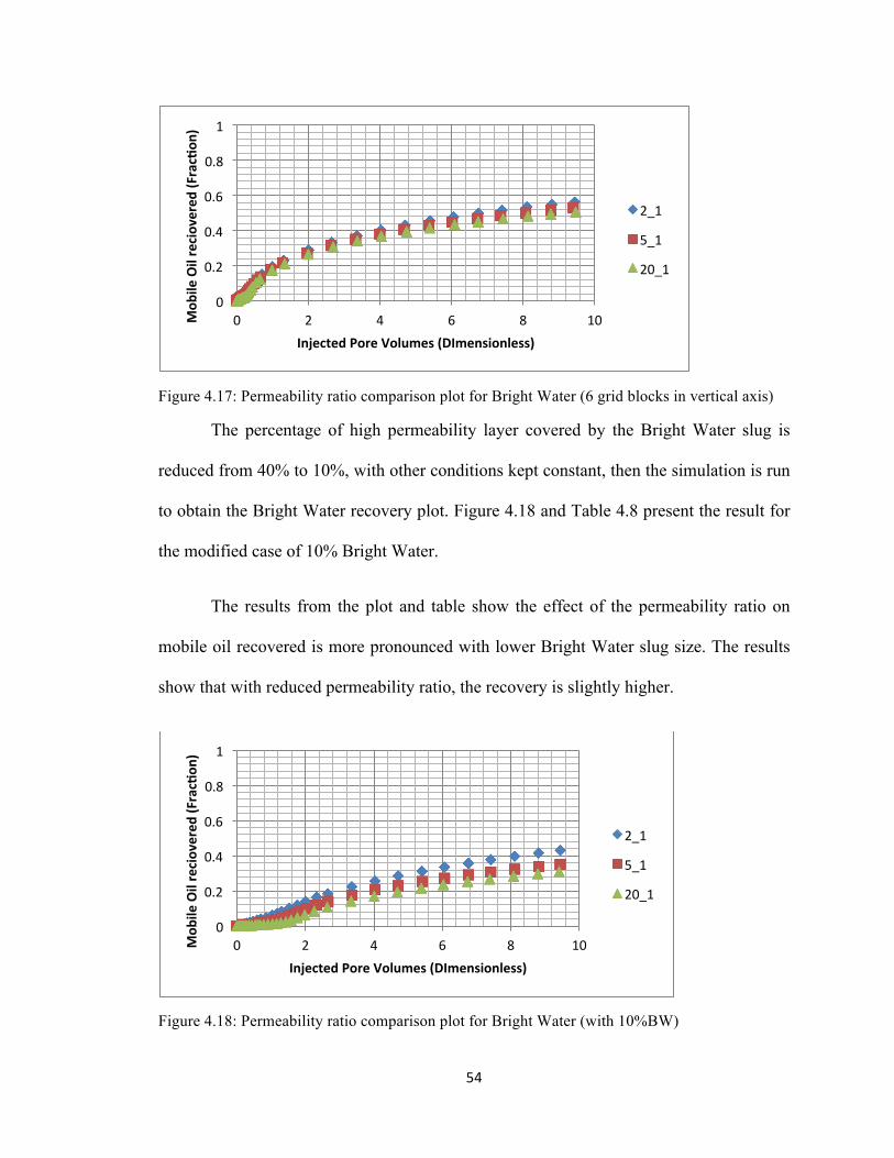
54
Figure 4.17: Permeability ratio comparison plot for Bright Water (6 grid blocks in vertical axis) The percentage of high permeability layer covered by the Bright Water slug is
reduced from 40% to 10%, with other conditions kept constant, then the simulation is run
to obtain the Bright Water recovery plot. Figure 4.18 and Table 4.8 present the result for
the modified case of 10% Bright Water.
The results from the plot and table show the effect of the permeability ratio on
mobile oil recovered is more pronounced with lower Bright Water slug size. The results
show that with reduced permeability ratio, the recovery is slightly higher.
Figure 4.18: Permeability ratio comparison plot for Bright Water (with 10%BW)
0
0.2
0.4
0.6
0.8
1
0 2 4 6 8 10 Mob
ile Oil reciovered
(Frac%on
)
Injected Pore Volumes (DImensionless)
2_1
5_1
20_1
0
0.2
0.4
0.6
0.8
1
0 2 4 6 8 10 Mob
ile Oil reciovered
(Frac%on
)
Injected Pore Volumes (DImensionless)
2_1
5_1
20_1
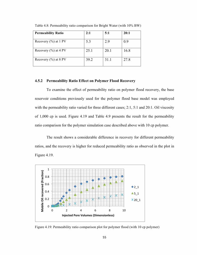
55
Table 4.8: Permeability ratio comparison for Bright Water (with 10% BW) Permeability Ratio 2:1 5:1 20:1
Recovery (%) at 1 PV 5.3 2.9 0.9
Recovery (%) at 4 PV 25.1 20.1 16.8
Recovery (%) at 8 PV 39.2 31.1 27.8
4.5.2 Permeability Ratio Effect on Polymer Flood Recovery
To examine the effect of permeability ratio on polymer flood recovery, the base
reservoir conditions previously used for the polymer flood base model was employed
with the permeability ratio varied for three different cases; 2:1, 5:1 and 20:1. Oil viscosity
of 1,000 cp is used. Figure 4.19 and Table 4.9 presents the result for the permeability
ratio comparison for the polymer simulation case described above with 10 cp polymer.
The result shows a considerable difference in recovery for different permeability
ratios, and the recovery is higher for reduced permeability ratio as observed in the plot in
Figure 4.19.
Figure 4.19: Permeability ratio comparison plot for polymer flood (with 10 cp polymer)
0
0.2
0.4
0.6
0.8
1
0 2 4 6 8 10 Mob
ile Oil recovered (Frac%on
)
Injected Pore Volumes (Dimensionless)
2_1
5_1
20_1
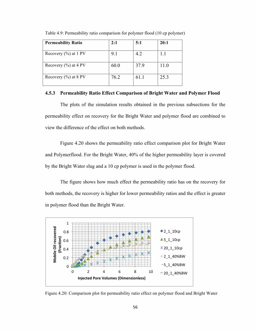
56
Table 4.9: Permeability ratio comparison for polymer flood (10 cp polymer)
Permeability Ratio 2:1 5:1 20:1
Recovery (%) at 1 PV 9.1 4.2 1.1
Recovery (%) at 4 PV 60.0 37.9 11.0
Recovery (%) at 8 PV 76.2 61.1 25.3
4.5.3 Permeability Ratio Effect Comparison of Bright Water and Polymer Flood
The plots of the simulation results obtained in the previous subsections for the
permeability effect on recovery for the Bright Water and polymer flood are combined to
view the difference of the effect on both methods.
Figure 4.20 shows the permeability ratio effect comparison plot for Bright Water
and Polymerflood. For the Bright Water, 40% of the higher permeability layer is covered
by the Bright Water slug and a 10 cp polymer is used in the polymer flood.
The figure shows how much effect the permeability ratio has on the recovery for
both methods, the recovery is higher for lower permeability ratios and the effect is greater
in polymer flood than the Bright Water.
Figure 4.20: Comparison plot for permeability ratio effect on polymer flood and Bright Water
0
0.2
0.4
0.6
0.8
1
0 2 4 6 8 10
Mob
ile Oil recovered
(Frac%on
)
Injected Pore Volumes (Dimensionless)
2_1_10cp
5_1_10cp
20_1_10cp
2_1_40%BW
5_1_40%BW
20_1_40%BW

57
CHAPTER 5
ECONOMICS CONSIDERATIONS
For the conclusion of this study, financial comparison is made between polymer
flood and the Bright Water treatment methods. A basic form of cost comparison is
employed in order to determine how the costs relate under different conditions. The price
of normal polymer; hydrolyzed polyacrylamide (HPAM) is between $0.9/lb to $2.0/lb15,
and the Bright Water polymer costs around 5 times as much as that for HPAM
(discussion with R.S. Seright, August 2010). Three price situations are considered for the
normal polymer and Bright Water polymer costs comparison:
i. Normal Case: Bright Water polymer costs five times as much as normal polymer.
ii. Optimistic Case: Bright Water polymer costs twice as much as normal polymer.
iii. Extremely Optimistic Case: Bright Water polymer costs the same as normal
polymer.
5.1 Bright Water Polymer Concentration
The concentration for the Bright Water polymer in injected water is 10,000 ppm
(i.e. 1%), and since the Bright Water injection is performed once in the operation - before
further water injection - the cost associated with the two major amounts of Bright Water
used in the course of this research is calculated once.
The two major Bright Water cases examined in this research are; when 40% of
high permeability layer is covered by Bright Water, and when 80% of high permeability
layer is covered by Bright Water.
58
5.1.1 Bright Water for 40% of High Permeability Layer
From the simulation model used in this study, the pore volume of each layer is
750 cubic meters, so 40% of the high permeability layer equals 300 cubic meters. This is
based on the optimistic assumption that all the Bright Water injected goes directly into
the high permeability layer as intended. The mass of Bright Water polymer involved (by
weight) can be calculated thus:
Bright Water polymer mass in 40% injection = kgmmkg 3000300001.010000 3
3 =××
5.1.2 Bright Water for 80% of High Permeability Layer
80% of the high permeability layer is 600 cubic meters. This is again based on the
optimistic assumption that all the Bright Water injected goes directly into the high
permeability layer as intended. The mass of Bright Water polymer involved can be
calculated thus:
Bright Water polymer mass in 80% injection kgmmkg 6000600001.010000 3
3 =××
Three price situations are to be examined regarding the relation of the cost of
Bright Water polymer and normal (HPAM) polymer.

59
5.2 Polymer (HPAM) Concentration
As given in the simulation model for the Bright Water treatment case, the pore
volume for each layer is 750 cubic meters, thus the total pore volume of the reservoir
model is 1500 cubic meters. The concentration of different polymer viscosities is
calculated based on the following HPAM polymer concentration in parts per million15:
10 cp = 900 ppm
100 cp = 3,000 ppm
1,000 cp = 10,000 ppm
10 cp Polymer
10 cp polymer mass in 1 PV kgmmkg 13501500001.0900 3
3 =××=
2 PV = 2700 kg, 3 PV = 4050 kg
100 cp Polymer
100 cp polymer mass in 1 PV kgmmkg 45001500001.03000 3
3 =××=
2 PV = 9000 kg, 3 PV =13500 kg
1000 cp Polymer
1000 cp polymer mass in 1 PV kgmmkg 150001500001.010000 3
3 =××=
2 PV = 30000 kg, 3 PV = 45000 kg
60
5.3 Cost Comparison for Bright Water and Polymer Flood
The cost of Bright Water polymer used is compared to that of normal polymer at
different pore volumes of polymer injected and for different oil and polymer viscosities
based on the recovery results from the simulator. The effect of the cost of water handling
for both processes is neglected as this is assumed approximately equal for both processes.
This comparison is made for oil of 10 cp, 100 cp, 1,000 cp and 10,000 cp
viscosities. This is done for different situations when the Bright Water polymer costs five
times as much as normal polymer, twice as much as normal polymer and the same as
normal polymer.
5.3.1 Normal Case Comparison
For this case, the Bright Water Polymer costs five times as much as the normal
polymer. The normal (HPAM) polymer costs $3.3 per kilogram and the Bright Water
polymer costs five times as much as this, which is $16.5 per kilogram.
For the comparison, a benefit ratio index is calculated by the relation below:
Benefit ratio = (percentage of oil recovered) / (cost of polymer or Bright Water injected)
Cost of normal polymer = Amount of polymer (kg) x $3.3/kg
Cost of Bright Water polymer = Amount of Bright Water polymer (kg) x $16.5/kg
Tables 5.1 through to 5.4 present the results the benefit ratio for cost comparison
of different oil viscosities. The comparison is made up to 3 PV of injection. The recovery
values are obtained from the tables of results in the previous chapter.
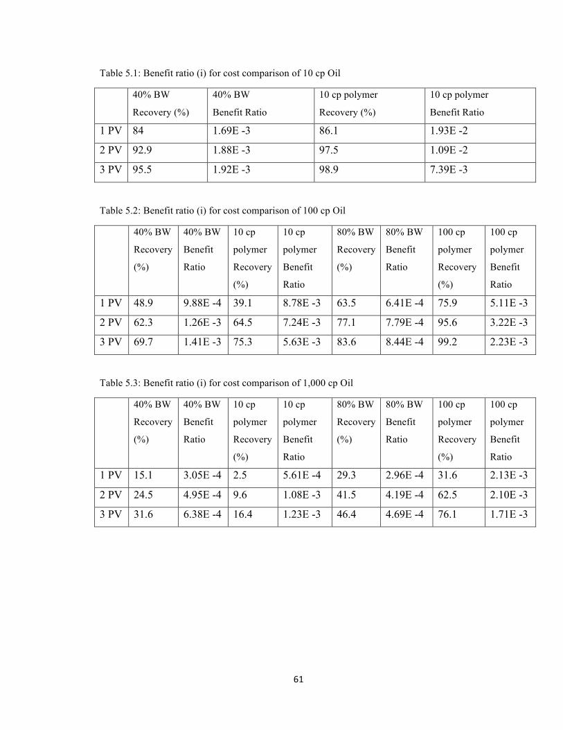
61
Table 5.1: Benefit ratio (i) for cost comparison of 10 cp Oil 40% BW
Recovery (%)
40% BW
Benefit Ratio
10 cp polymer
Recovery (%)
10 cp polymer
Benefit Ratio
1 PV 84 1.69E -3 86.1 1.93E -2
2 PV 92.9 1.88E -3 97.5 1.09E -2
3 PV 95.5 1.92E -3 98.9 7.39E -3
Table 5.2: Benefit ratio (i) for cost comparison of 100 cp Oil 40% BW
Recovery
(%)
40% BW
Benefit
Ratio
10 cp
polymer
Recovery
(%)
10 cp
polymer
Benefit
Ratio
80% BW
Recovery
(%)
80% BW
Benefit
Ratio
100 cp
polymer
Recovery
(%)
100 cp
polymer
Benefit
Ratio
1 PV 48.9 9.88E -4 39.1 8.78E -3 63.5 6.41E -4 75.9 5.11E -3
2 PV 62.3 1.26E -3 64.5 7.24E -3 77.1 7.79E -4 95.6 3.22E -3
3 PV 69.7 1.41E -3 75.3 5.63E -3 83.6 8.44E -4 99.2 2.23E -3
Table 5.3: Benefit ratio (i) for cost comparison of 1,000 cp Oil 40% BW
Recovery
(%)
40% BW
Benefit
Ratio
10 cp
polymer
Recovery
(%)
10 cp
polymer
Benefit
Ratio
80% BW
Recovery
(%)
80% BW
Benefit
Ratio
100 cp
polymer
Recovery
(%)
100 cp
polymer
Benefit
Ratio
1 PV 15.1 3.05E -4 2.5 5.61E -4 29.3 2.96E -4 31.6 2.13E -3
2 PV 24.5 4.95E -4 9.6 1.08E -3 41.5 4.19E -4 62.5 2.10E -3
3 PV 31.6 6.38E -4 16.4 1.23E -3 46.4 4.69E -4 76.1 1.71E -3

62
Table 5.4: Benefit ratio (i) for cost comparison of 10,000 cp Oil 40% BW
Recovery
(%)
40% BW
Benefit
Ratio
100 cp
polymer
Recovery
(%)
100 cp
polymer
Benefit
Ratio
80% BW
Recovery
(%)
80% BW
Benefit
Ratio
1,000 cp
polymer
Recovery
(%)
1,000 cp
polymer
Benefit
Ratio
1 PV 1.8 3.64E -5 1.9 1.28E -4 12.1 1.22E -4 36.2 7.31E -4
2 PV 2.7 5.45E -5 6.4 2.15E -4 18.7 1.89E -4 67.3 6.79E -4
3 PV 5.1 1.03E -4 12.5 2.81E -4 23.9 2.41E -4 78.2 5.27E -4
The results from the tables above show the polymer flood to be more profitable
than Bright Water for this case. For example; at 1 PV of injection for the 10 cp oil, the
Bright Water (40% BW) benefit ratio was 1.69E-3 and the 10 cp polymer benefit ratio
was 1.93E-2 (highest benefit ratio for this oil viscosity) therefore showing the polymer
flood at this point to be 11.42 times more profitable than Bright Water. At 3 PV, the
polymer flood is 3.84 times more profitable than Bright Water.
For 100 cp oil, the highest benefit ratio was 8.78E-3 - from the 10 cp polymer at 1
PV with 39.1% mobile oil recovered. The highest benefit ratio from Bright Water was
1.41E-3 - from the 40% BW at 3 PV of injection, 69.7% of mobile oil was recovered at
this point. The 100 cp polymer gave the highest recovery of 99.2% at 3 PV with a benefit
ratio of 2.23E-3.
For 1,000 cp oil, the highest benefit ratio was 2.13E-3 from the 100 cp polymer at
1 PV of injection and 31.6% mobile oil recovered. For 10,000 cp oil, the highest benefit
ratio was 7.31E-4 - from 1,000 cp polymer at 1 PV with 36.2% mobile oil recovered.
It is observed that the profitability of the polymer flood over Bright Water
decreases with higher pore volumes of injection, this is due to the fact that the Bright
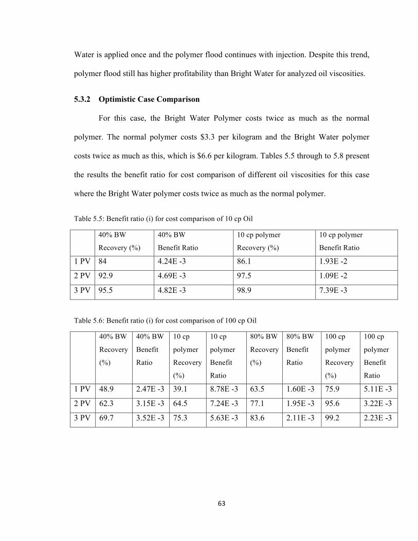
63
Water is applied once and the polymer flood continues with injection. Despite this trend,
polymer flood still has higher profitability than Bright Water for analyzed oil viscosities.
5.3.2 Optimistic Case Comparison
For this case, the Bright Water Polymer costs twice as much as the normal
polymer. The normal polymer costs $3.3 per kilogram and the Bright Water polymer
costs twice as much as this, which is $6.6 per kilogram. Tables 5.5 through to 5.8 present
the results the benefit ratio for cost comparison of different oil viscosities for this case
where the Bright Water polymer costs twice as much as the normal polymer.
Table 5.5: Benefit ratio (i) for cost comparison of 10 cp Oil 40% BW
Recovery (%)
40% BW
Benefit Ratio
10 cp polymer
Recovery (%)
10 cp polymer
Benefit Ratio
1 PV 84 4.24E -3 86.1 1.93E -2
2 PV 92.9 4.69E -3 97.5 1.09E -2
3 PV 95.5 4.82E -3 98.9 7.39E -3
Table 5.6: Benefit ratio (i) for cost comparison of 100 cp Oil 40% BW
Recovery
(%)
40% BW
Benefit
Ratio
10 cp
polymer
Recovery
(%)
10 cp
polymer
Benefit
Ratio
80% BW
Recovery
(%)
80% BW
Benefit
Ratio
100 cp
polymer
Recovery
(%)
100 cp
polymer
Benefit
Ratio
1 PV 48.9 2.47E -3 39.1 8.78E -3 63.5 1.60E -3 75.9 5.11E -3
2 PV 62.3 3.15E -3 64.5 7.24E -3 77.1 1.95E -3 95.6 3.22E -3
3 PV 69.7 3.52E -3 75.3 5.63E -3 83.6 2.11E -3 99.2 2.23E -3
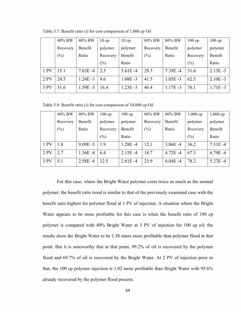
64
Table 5.7: Benefit ratio (i) for cost comparison of 1,000 cp Oil 40% BW
Recovery
(%)
40% BW
Benefit
Ratio
10 cp
polymer
Recovery
(%)
10 cp
polymer
Benefit
Ratio
80% BW
Recovery
(%)
80% BW
Benefit
Ratio
100 cp
polymer
Recovery
(%)
100 cp
polymer
Benefit
Ratio
1 PV 15.1 7.63E -4 2.5 5.61E -4 29.3 7.39E -4 31.6 2.13E -3
2 PV 24.5 1.24E -3 9.6 1.08E -3 41.5 1.05E -3 62.5 2.10E -3
3 PV 31.6 1.59E -3 16.4 1.23E -3 46.4 1.17E -3 76.1 1.71E -3
Table 5.8: Benefit ratio (i) for cost comparison of 10,000 cp Oil 40% BW
Recovery
(%)
40% BW
Benefit
Ratio
100 cp
polymer
Recovery
(%)
100 cp
polymer
Benefit
Ratio
80% BW
Recovery
(%)
80% BW
Benefit
Ratio
1,000 cp
polymer
Recovery
(%)
1,000 cp
polymer
Benefit
Ratio
1 PV 1.8 9.09E -5 1.9 1.28E -4 12.1 3.06E -4 36.2 7.31E -4
2 PV 2.7 1.36E -4 6.4 2.15E -4 18.7 4.72E -4 67.3 6.79E -4
3 PV 5.1 2.58E -4 12.5 2.81E -4 23.9 6.04E -4 78.2 5.27E -4
For this case; where the Bright Water polymer costs twice as much as the normal
polymer, the benefit ratio trend is similar to that of the previously examined case with the
benefit ratio highest for polymer flood at 1 PV of injection. A situation where the Bright
Water appears to be more profitable for this case is when the benefit ratio of 100 cp
polymer is compared with 40% Bright Water at 3 PV of injection for 100 cp oil; the
results show the Bright Water to be 1.58 times more profitable than polymer flood at that
point. But it is noteworthy that at that point, 99.2% of oil is recovered by the polymer
flood and 69.7% of oil is recovered by the Bright Water. At 2 PV of injection prior to
that, the 100 cp polymer injection is 1.02 more profitable than Bright Water with 95.6%
already recovered by the polymer flood process.
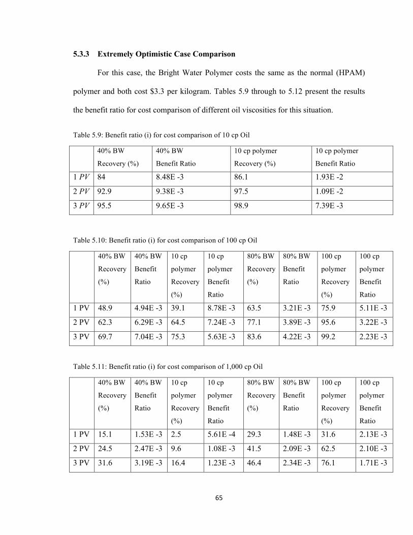
65
5.3.3 Extremely Optimistic Case Comparison
For this case, the Bright Water Polymer costs the same as the normal (HPAM)
polymer and both cost $3.3 per kilogram. Tables 5.9 through to 5.12 present the results
the benefit ratio for cost comparison of different oil viscosities for this situation.
Table 5.9: Benefit ratio (i) for cost comparison of 10 cp Oil 40% BW
Recovery (%)
40% BW
Benefit Ratio
10 cp polymer
Recovery (%)
10 cp polymer
Benefit Ratio
1 PV 84 8.48E -3 86.1 1.93E -2
2 PV 92.9 9.38E -3 97.5 1.09E -2
3 PV 95.5 9.65E -3 98.9 7.39E -3
Table 5.10: Benefit ratio (i) for cost comparison of 100 cp Oil 40% BW
Recovery
(%)
40% BW
Benefit
Ratio
10 cp
polymer
Recovery
(%)
10 cp
polymer
Benefit
Ratio
80% BW
Recovery
(%)
80% BW
Benefit
Ratio
100 cp
polymer
Recovery
(%)
100 cp
polymer
Benefit
Ratio
1 PV 48.9 4.94E -3 39.1 8.78E -3 63.5 3.21E -3 75.9 5.11E -3
2 PV 62.3 6.29E -3 64.5 7.24E -3 77.1 3.89E -3 95.6 3.22E -3
3 PV 69.7 7.04E -3 75.3 5.63E -3 83.6 4.22E -3 99.2 2.23E -3
Table 5.11: Benefit ratio (i) for cost comparison of 1,000 cp Oil 40% BW
Recovery
(%)
40% BW
Benefit
Ratio
10 cp
polymer
Recovery
(%)
10 cp
polymer
Benefit
Ratio
80% BW
Recovery
(%)
80% BW
Benefit
Ratio
100 cp
polymer
Recovery
(%)
100 cp
polymer
Benefit
Ratio
1 PV 15.1 1.53E -3 2.5 5.61E -4 29.3 1.48E -3 31.6 2.13E -3
2 PV 24.5 2.47E -3 9.6 1.08E -3 41.5 2.09E -3 62.5 2.10E -3
3 PV 31.6 3.19E -3 16.4 1.23E -3 46.4 2.34E -3 76.1 1.71E -3

66
Table 5.12: Benefit ratio (i) for cost comparison of 10,000 cp Oil 40% BW
Recovery
(%)
40% BW
Benefit
Ratio
100 cp
polymer
Recovery
(%)
100 cp
polymer
Benefit
Ratio
80% BW
Recovery
(%)
80% BW
Benefit
Ratio
1,000 cp
polymer
Recovery
(%)
1,000 cp
polymer
Benefit
Ratio
1 PV 1.8 1.82E -4 1.9 1.28E -4 12.1 6.11E -4 36.2 7.31E -4
2 PV 2.7 2.73E -4 6.4 2.15E -4 18.7 9.44E -4 67.3 6.79E -4
3 PV 5.1 5.15E -4 12.5 2.81E -4 23.9 1.21E -3 78.2 5.27E -4
For this extremely optimistic case, the polymer flood has higher benefit ratios for
10 cp and 100 cp oil, but the Bright Water has higher benefit ratios for the 1,000 cp and
10,000 cp oil. At 1 PV of injection, the polymer flood for all oil viscosities investigated
has higher benefit ratios than Bright Water. With continued injection the benefit ratio of
Bright Water increases; and for the highly viscous oil of 1,000cp and 10,000 cp the
benefit ratio becomes higher than that of the polymer flood after 2 PV of injection.
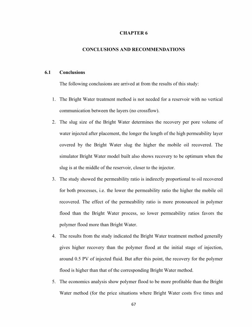
67
CHAPTER 6
CONCLUSIONS AND RECOMMENDATIONS
6.1 Conclusions
The following conclusions are arrived at from the results of this study:
1. The Bright Water treatment method is not needed for a reservoir with no vertical
communication between the layers (no crossflow).
2. The slug size of the Bright Water determines the recovery per pore volume of
water injected after placement, the longer the length of the high permeability layer
covered by the Bright Water slug the higher the mobile oil recovered. The
simulator Bright Water model built also shows recovery to be optimum when the
slug is at the middle of the reservoir, closer to the injector.
3. The study showed the permeability ratio is indirectly proportional to oil recovered
for both processes, i.e. the lower the permeability ratio the higher the mobile oil
recovered. The effect of the permeability ratio is more pronounced in polymer
flood than the Bright Water process, so lower permeability ratios favors the
polymer flood more than Bright Water.
4. The results from the study indicated the Bright Water treatment method generally
gives higher recovery than the polymer flood at the initial stage of injection,
around 0.5 PV of injected fluid. But after this point, the recovery for the polymer
flood is higher than that of the corresponding Bright Water method.
5. The economics analysis show polymer flood to be more profitable than the Bright
Water method (for the price situations where Bright Water costs five times and

68
twice as much as normal polymer) up to 3 PV of injection investigated. After this,
at later stages of injection, the benefit ratio of Bright Water is greater than
polymer flood but most of the mobile oil would already have been recovered. For
the situation where the Bright Water polymer costs the same as normal polymer,
the Bright Water is more profitable than polymer flood for the highly viscous oil
of 1,000 cp and 10,000 cp.
6.2 Recommendations
The following recommendations are made for the possibility of future work to be
done in the analysis and comparison of Bright Water and polymer flood:
1. An analytical model could be developed for the Bright Water treatment method to
compare directly with the polymer flood analytical model.
2. For the simulation of the Bright Water case in this study, the Bright Water slug
placement was simulated directly by setting the porosity and permeability of the
length of high permeability layer to be blocked to zero. Further work can be done
in which the Bight Water placement is achieved by water injection and then
blocking the grid parts covered by this injection; this would give a more realistic
outcome and part of the Bright Water would flow into the lower permeability
zone before ‘popping’.
3. Further work could also be done on the simulation of both the polymer flood and
Bright Water processes with flexibility given to the saturation of reservoir fluids
before applying the enhanced oil recovery process. In this case, the lower
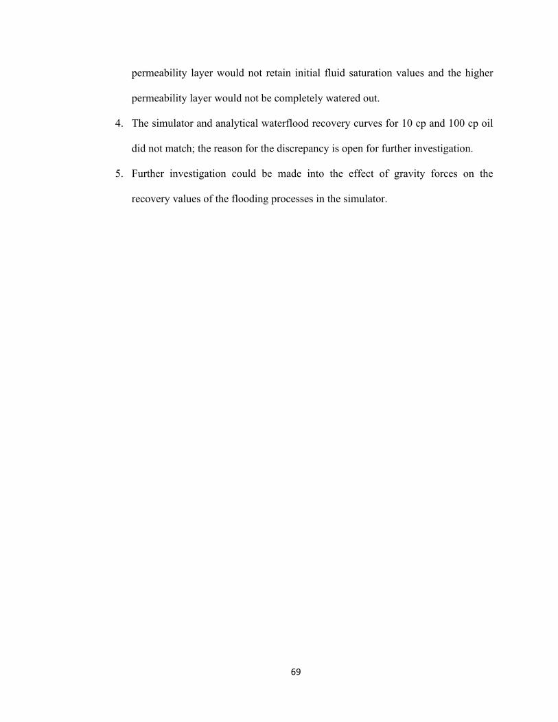
69
permeability layer would not retain initial fluid saturation values and the higher
permeability layer would not be completely watered out.
4. The simulator and analytical waterflood recovery curves for 10 cp and 100 cp oil
did not match; the reason for the discrepancy is open for further investigation.
5. Further investigation could be made into the effect of gravity forces on the
recovery values of the flooding processes in the simulator.
70
NOMENCLATURE
A = cross-sectional area perpendicular to flow lines, ft2
BL = Buckley-Leverett
BT = Breakthrough
BW = Bright Water
c2 = 0.0011271; 2πc2 = 0.00708; 1/(2πc2) = 141.2
fo = qo/qt, fractional flow of oil flow in the total flow stream, sandface conditions, frac.
fw = qw/qt, fractional flow of water flow in the total flow stream, sandface conditions, frac.
fwf = fractional flow of water at the flood front, sandface conditions, frac.
fwe = fractional flow in the total flow stream at the producing (exit) sandface, frac.
f’w = dfw/dSw, first derivative of the fractional-flow (of water)
f’wBT = (dfw/dSw)SwBT, first derivative of the fractional-flow (of water) evaluated at Swf
f’wf = (dfw/dSw)Swf, first derivative of the fractional-flow (of water) evaluated at Swf
f’we = (dfw/dSw)Sw2 first derivative of the fractional-flow (of water) evaluated at Swe
k = absolute permeability, mD
kj = phase-j effective permeability, mD
kro = relative permeability to oil, frac.
krw = relative permeability to water, frac.
L = flood length; injector-to-producer distance, ft
M = mobility ratio, ratio of the mobility of the displacing fluid to the mobility of the displaced fluid, dimensionless

71
M0 = end-point mobility ratio, ratio of the end-point mobility of the displacing fluid to the end-point mobility of the displaced fluid, dimensionless
no = shape parameter of oil relative permeability, dimensionless
nw = shape parameter of water relative permeability, dimensionless
Nc = capillary number, dimensionless
Ng = gravity number, dimensionless
pc = capillary pressure, psi
po = oil capillary pressure, psi
pw = water pressure, psi
PV = pore volumes
qo = oil flow rate at sandface, rb/d
qt = total (qo + qw) flow rate at sandface, rb/d
qw = water flow rate at sandface, rb/d
Soi = initial oil saturation, frac.
Sor = residual oil saturation, frac.
Sw = water saturation, frac.
Swavg = average water saturation (behind-the-front if before-breakthrough and in-the-reservoir if after-breakthrough), frac.
SwBT = water saturation of the flood front at the time of breakthrough, frac.
Swe = water saturation at the producing (exit) sandface, frac.
Swf = water saturation at the flood front, frac.
Swi = initial water saturation, frac.
Swr = residual water saturation, frac.
t = time, days
uo = oil velocity at sandface, ft/d
ut = uo + uw, total velocity at sandface, ft/d

72
uw = water velocity at sandface, ft/d
v = u/ Φ, “true or interstitial” velocity, ft/d
Vp = initial pore volume, rb
vt = qt/A, total velocity at sandface, (rb/d)/ft2
w = flood width, ft
Wi = cumulative water injected at sandface, rb
WiD = Wi/Vp, dimensionless number of pore volumes of cumulative water injected
WiDBT = dimensionless number of pore volumes (PV) of cumulative water injected at the time of breakthrough (BT)
x = distance along flow direction, ft
θ = formation dip angle (positive for counterclockwise from the horizontal), deg.
λo = ko/µo, mobility of oil, mD/cP
λt = λo + λw , total mobility, mD/cP
λw = kw/µw, mobility of water, mD/cP
µo = oil viscosity, cP
µw = water viscosity, cP
ρo = density of oil at reservoir conditions, lbm/ft3
ρw = density of water at reservoir conditions, lbm/ft3
∆ρ = ρw – ρo, lbm/ft3
Φ = porosity, frac.

73
REFERENCES
1. Seright, R.S. 1988. Placement of Gels to Modify Injection Profiles. Paper
SPE/DOE 17332 prepared for presentation at the SPE/DOE Enhanced Oil
Recovery Symposium held in Tulsa, Oklahoma, 17-20 April.
2. Frampton H. et al. 2004. Development of a Novel Waterflood Conformance
Control System. Paper SPE 89391 presented at the 2004 SPE/DOE Fourteenth
Symposium on Improved Oil Recovery held in Tulsa, Oklahoma, USA, 17-21
April.
3. Pritchett J. et al. 2003. Field Application of New In-depth Waterflood
Conformance Improvement Tool. Paper SPE 84897 presented at the SPE
International Conference on Improved Oil Recovery in Asia Pacific, Kuala
Lumpur, Malaysia, 20-21 October.
4. Sorbie K.S. and Seright R.S. 1992. Gel Placement in Heterogeneous Systems with
Crossflow. Paper SPE/DOE 24192 presented at the SPE/DOE Eight Symposium
on Enhanced Oil Recovery held in Tulsa, Oklahoma, 22-24 April.
5. Root, P.J. and Skiba, F.F. Crossflow Effects During an Idealized Displacement
Process in a Stratified Reservoir. (Sept. 1965) SPEJ 229-237.
6. “Near-Wellbore Technology” Brochure 1024-87TL, Phillips Petroleum Co.,
Bartlesville, OK (1987).
7. Seright R.S. 1990. Impact of Dispersion on Gel Placement for Profile Control.
Paper SPE 20127 first presented at the SPE Permian Basin and Gas Recovery
Conference held in Midland, 8-9 March.
8. Lake, L.W, Enhanced Oil Recovery. Prentice-Hall, Inc. New Jersey. 1989.
74
9. Green D.W., and Willhite G.P., Enhanced Oil recovery. SPE textbook series
vol.6. SPE, Richardson, Texas. 1998.
10. Ohms, D.S., McLeod, J., graff, C.J., Frampton, H., Chang, K.T., Morgan, J.C,
Cheung, S., and Yancey, K. 2009. Incremental Oil Success from Waterflood
Sweep Improvement in Alaska. Paper SPE 121761 prepared for presentation at
the 2009 International Symposium on Oilfield Chemistry, The Woodland, TX,
20-22 April.
11. Frampton H. et al. 2009. Bright WaterTM Sweep Improvement from the Lab to the
Field. Paper presented at the 15th European Symposium on Improved Oil
Recovery – Paris, France, 27-29 April.
12. Her-Yuan Chen, Engineering Reservoir Mechanics. New Mexico Tech, 2009.
13. Oppong, K. 2009. Polymerflood Simulation in a Heterogeneous Idealized
Reservoir with or without Crossflow. New Mexico Tech, December.
14. Seright R.S. Spreadsheets for Polymer Flooding Fractional Flow Calculations”
http://baervan.nmt.edu/randy/home.html
15. Seright R.S. 2010. Potential for Polymer Flooding Reservoirs with Viscous Oils.
Paper SPE 129899 prepared for presentation at the 2010 SPE Improved Oil
Recovery Symposium held in Tulsa, Oklahoma, USA, 24-28 April.
16. Morgan, N., “Pop Goes the Polymer”, BP Frontiers. December 2007.

75
APPENDIX A: Description of the Basic Reservoir Simulation Model.
A.1 Case Definition:
This is section where the basic tasks are defined for the simulator. The Black-Oil-
Model is selected with Water and Oil as the reservoir fluids. Cartesian, CornerPoint is
selected for geometry option and model dimensions: x-y-z = 50-1-2. Vertical
Equilibrium is activated under the SCAL tab with Fully Implicit solution option
selected.
A.2 Grid
The basic geometry of the simulation grid and various rock properties (porosity,
absolute permeability, etc) in each grid cell are specified in the grid section. From these
properties, the simulator calculates the pore volumes of the grid blocks and the inter-
block transmissibilities. The keywords used in this section usually depend on the
geometry option selected in the initialization section. In this case, the Cartesian-
ConerPoint geometry option was used with the grid block coordinate lines and grid block
corner keywords defined for the reservoir model. The porosity distribution in the
reservoir is assumed to be homogeneous with a porosity of 0.30 while the permeability is
homogeneous within each layer with values of 100md for layer 1 and 1000md for layer
2.
A.3 PVT Properties of the Reservoir Fluids
This section of the input data contains pressure and saturation dependent
properties of the reservoir fluids and rocks. The reservoir fluids are oil and water which
are incompressible. The oil contains no concentration of dissolved gas. At a reference
76
pressure of 78atm the oil has a viscosity ranging 1 to105 cp as specified in Table 3.1. The
oil formation volume factor, water (Bw) and oil (Bo) both equal to 1. The bulk
compressibility of the rock was set at 2 x E-8 atm-1. This value was picked from the work
done from similar studies.
A.4 SCAL (saturation Section)
Corey correlation was used to obtain the relative permeability curve with Corey
exponent with respect oil and water both equal to 2. The vertical equilibrium option was
used to modify the relative permeability curve into pseudo-relative permeability for the
crossflow modes. The irreducible water and oil saturation was set to 0.3.
A.5 Initialization
This section contains input data for the initial state of the reservoir. The pressure
at the datum depth was set at 78.6atm with oil- water capillary pressure set to 0 atm. The
initial fluid saturations were also defined under this section, with 0.7 and 0.3 for oil and
water saturations respectively.
A.6 Schedule
This contains information regarding scheduling producers and injector for
production and injection. The wells (producer and injector) were scheduled to operate for
a three week period with constant control settings. The injector well is located in the
center of cells (1, 1, 1) and the producer in the cell (50, 1, 1) of the grid. The wells were
set to perforate through the entire thickness of the formation. The injector wells were
constraints to operate at maximum injection pressure of 78.6 atm and injection rate of
77
100 cubic meters per day. Same time, the minimum allowable bottom hole pressure for
the production well was set at 12 atm but same rate control. These controls were slightly
varied in the polymer injection operation and also in the horizontal well injection for the
sake of injectivity.
A.7 Summary
This section specifies a number of variables that are to be written to Summary
files after each time step of the simulation. The oil production total and water injection
total were the most important variables selected for the oil recovery vs. pore volumes of
water injection plots.
78
APPENDIX B: Description of the Polymer Model Keywords.
B.1 Case Section
The polymer option was selected under the PVT tab
B.2 PVT Section
Three keywords were selected under this section with the activation of the
polymer option under the PVT tab in the Case section.
Polymer Solution Viscosity (PLYVISC): This keyword is only used for polymer studies
where the salt sensitivity is not activated. The polymer concentration is defined by
relating the mass concentration (in kg/m3) to the viscosity (in cp). The following entries
were made for the polymer concentration: 0 kg/m3 – 1 cp, 0.9 kg/m3 – 10 cp, 3 kg/m3 –
100 cp and 10 kg/m3 – 1,000 cp.
Polymer/Salt Concentration for Mixing Calculations (PLYMAX): The value of
polymer concentration in the solution which is to be used in the calculation of the
maximum polymer fluid component viscosity. An entry of 12 kg/m3 was made.
Todd-Longstaff Mixing Parameter (TLMIXPAR): Mixing parameter for viscosity
calculation, the value of this parameter for each miscibility region ranges from 0.0 to 1.0.
1.0 is selected for maximum miscibility between the polymer and water.
B.3 SCAL Section
Two keywords are selected under this section for the description of polymer-rock
properties, the entries are made to have the polymer properties similar to that of water as
much as possible – excluding viscosity.
79
Polymer Rock Properties (PLYROCK): Comprises data specifying the rock properties
which are required for the polymer flood model. The following entries were made: Dead
pore space: 0, Residual resistance factor for rock type: 1, Mass density of rock type
(reservoir conditions): 500 kg/m3, adsorption index: 0.0035.
Polymer Adsorption Functions (PLYADS): Describes polymer adsorption functions by
the rock formation. It relates the local polymer concentration in the solution surrounding
the rock (in kg/m3) to the corresponding saturated concentration of polymer adsorbed by
the rock formation (in kg/kg). 0 kg/m3 – 0 kg/kg, 2 kg/m3 – 0.0015 kg/kg, 8 kg/m3 –
0.0025 kg/kg.
B.4 Schedule Section
Polymer/Salt Concentrations for Injection Wells (WPOLYMER): This
keyword is used to specify the concentration of polymer and salt in the injection stream
of each well. The appropriate concentration is specified for the corresponding polymer
viscosity as given in B.2.