analysis of categorical data for … of categorical data for crossover designs. (under the direction...

ANALYSIS OF CATEGORICAL DATA FOR CROSSOVER DESIGNS

by

Susan Shearer Atkinson

Department of BiostatisticsUniversity of North Carolina at Chapel Hill, NC

Institute of Mimeo Series No. 1882TJuly 1990

ANALYSIS OF CATEGORICAL DATA

FOR CROSSOVER DESIGNS

by

Susan Shearer Atkinson

A Dissertation submitted to the faculty of the University ofNorth Carolina at Chapel Hill in partial fulfillment of therequirements for the degree of Doctor of Philosophy in the

Department of Biostatistics.

Chapel Hill, 1990

Reader

cL •.r-D~J~Reader

· ABSTRACT

SUSAN SHEARER ATKINSON. Analysis of Categorical Data For Crossover

Designs. (Under the direction of GARY G. KOCH).

For the crossover design, subjects receive a random sequence of treatments

across multiple periods. This research focuses on those situations where the

outcome is categorical. Gart's (1969) method for the classical 2 x 2 crossover

design with a binary response is extended to encompass more general

crossover designs. Log-linear regression models are applied to the conditional

joint probabilities for discordant sets of outcomes in this method; the parameters

are defined relative to subject-specific, marginal probabilities.

This method applies to nominal and ordinal outcomes. The modeling also

allows for any number of periods or of treatments and applies to any structure of

sequence groups. Furthermore, inclusion of covariates (even those that are time

dependent), baseline periods, and semi-ordinal data with survival structure is

possible.

The subject effects can be considered fixed or random as they are cancelled

out through creation of conditioned sets. These sets for some crossover designs

have a varying number of components. A log-linear model for outcomes with

varying length response vectors was developed to handle this situation. This

method also allows consideration of missing data. The assumption of

independence across the periods is assessed through lack of fit of this model.

Adjustments for potential lack of fit have been specified through association

parameters which measure correlation within subjects across the periods.

Furthermore, association by sequence group interactions are considered which

fully specify the available vector space for analysis.

The method of Kenward and Jones (1989), where parameters are defined

and analysis accomplished on the joint probabilities for combinations of

outcomes across all periods, also considers association parameters. The

similar aspects of their strategy to the proposed one is explored along with the

limitations it presents. The method of Stram, Wei and Ware (1988) for

population marginal probabilities is also considered and its extension to

crossover designs is applied.

Finally, a pairwise period ratio method is developed from the same marginal

probabilities as with the Gart model. Analysis is performed with weighted least

squares. A least squares smoothing technique is applied to. the three ratio

functions to adjust for potential asymptotic multicollinearity among these

estimates.

ACKNOWLEDGMENTS

I would like to thank my advisor, Dr. Gary G. Koch, for the guidance he has

provided on this dissertation. His help and support have been invaluable-and I

feel fortunate to have worked with him on this project. He has been readily

available to share ideas and clarify difficult statistical issues. I'm thankful for his

flexibility in accommodating my schedule, particularly working around the time

constraints I have as the mother of two. The completion of this work would have

not been possible except for his encouragement and support. I would also like

to express my sincere appreciation to my committee members: Drs. E. C. Davis,

L. Kupper, C. D.Turnbull and H. Heiss, for their encouragement and review of

chapters.

With deepest affection and appreciation, I thank my husband Doug for his

constant support and belief that I could finish this. I am thankful for the many

hours he spent printing and photocopying, his help with word processing

concerns, his suggestions for the simulation of Chapter 9, but most importantly

for his love. A special big hug goes to the lights in my life, Stephanie and

Melissa. They brighten my days with their sweetness and caring.

In all things I give thanks to God who guides me through life. With special

thanks and love, I remember my mother, Barbara H. Shearer. She passed away

a few months before seeing this completed but I know she is looking from her

heavenly home and smiling with satisfaction. The years of support and approval

from her provided me with the perseverance and confidence to accomplish this.

I also want to thank the rest of my family and friends for their warm support. I

also have great appreciation for Coral Jeffries and her expert typing of many of

the more difficult Tables.

Chapter

TABLE OF CONTENTS

Page

1. REVIEW OF CROSSOVER DESIGNS AND METHODS FOR THEIRANALYSIS 1

1.1 Overview of Crossover Designs

1.1.1 Definition1.1 .2 Range of Designs

1

12

1.2 Review of Methods for Two Period / Two Treatment / TwoSequence Crossover Designs 4

1.2.1 Literature review of methods for crossoverdesigns with continuous measures 5

1.2.2 Review of methods for crossover designs with thecategorical outcome 7

1.3 Review of Methods for Multi Period or Multi TreatmentDesigns 10

1.3.1 Continuous Outcomes1.3.2 Categorical Outcomes

1.4 Data Structure and Questions for Analysis

1.4.1 Data structure1.4.2 Relevant analysis issues

1.5 Overview of research

2. OVERVIEW OF CATEGORICAL DATA METHODS

2.1 General Approaches to Categorical Data

2.2 Randomization methods

2.3 Maximum likelihood methods for log-linear models

1111

12

1213

16

18

18

18

19

2.3.1 Maximum likelihood methods for ordinal data 222.3.2 Several Models of application to Crossover

Designs 25

2.4 Weighted least squares methods 27

2.4.1 Categorical Data methodology for repeatedmeasures 31

2.4.2 Application to Crossover Designs 35

3. LOGISTIC MODELS FOR TWO PERIOD CROSSOVER DESIGNSFOR COMPARISON OF TWO TREATMENTS FOCUSING ONDISCORDANT PAIRS 37

3.1 Introduction 37

3.2 Review of current methods 38

3.3 Classical two period, two treatment crossover 39

3.3.1 Gart's method revisited 393.3.2 Gart's method expressed in terms of logistic model 413.3.3 Inclusion of covariates 443.3.4 Extension of nominal outcome 453.3.5 Quasi-independence and the relationship to (j and t}

parameters 48 e3.3.6 Extension from nominal outcomes to ordinaloutcomes 52

3.3.7 Extensions to time dependent covariates 543.3.8 Extensions to partially ordered data for survival 55

3.4 Other two period, two treatment designs 59

3.4.1 2 periods / 2 treatments / 4 sequence groups 593.4.2 2 periods / 2 treatments / 3 sequence groups 65

3.5 Example 66

4. LOGISTIC MODELS FOR TWO PERIOD CROSSOVER DESIGNSFOR COMPARISON OF THREE TREATMENTS FOCUSING ONDISCORDANT PAIRS 70

4.1 Introduction 70

4.2 2 periods / 3 treatments / 3 sequence groups 70



4.5 Example 87

4.6 Discussion 91

5. LOGISTIC MODELS FOR THREE PERIOD CROSSOVER DESIGNSFOCUSING ON DISORDANT TRIPLES 92

5.1 Introduction 92

5.2 Gart type logistic model for binary response 93

5.3 Period association effects incorporated into the binary model 98

5.3.1 Definition of cr and t} parameters 98·5.3.2 Alternate parameterization 100

5.3.3 Jones and Kenward type of association parameters 1075.3.4 Summary of Association Parameters 1095.3.5 Alternate Method to relate Methods 1 and 2 110

5.4 Extension to nominal and ordinal outcomes 113

5.5 Logistic Model for Binary Response with two Latin squares 128

5.6 Example 130

6. LOGISTIC MODELS FOR FOUR PERIOD CROSSOVER DESIGNSFOCUSING ON DISCORDANT JOINT OUTCOMES 135

6.1 Introducti0 n 135

6.2 Logistic model for conditional partitions of binary response 136

6.3 Two-stage strategy 141

6.4 Log-linear model for multinomial with varying length responsevectors 142

6.5 Varying length response multinomial vectors applied to thefour period design 146

6.6 Period association effects incorporated into the binary model 148

6.7 Comparison of Jones and Kenward period associationeffects 149

6.8 Extension to nominal and ordinal responses 151

6.9 Application to baseline periods 155

6.10 Extension to double crossover 157

6.11 Four period example, binary response 160

7. LOGISTIC MODELS FOR CROSSOVER DESIGNS FOCUSING ONDISCORDANT SETS OF JOINT OUTCOMES INCORPORATING AMISSING DATA STRUCTURE 167

7.1 Introduction 167

7.2 General Notation 168

7.3 Strategy presented through a three period crossover design 168

7.3.1 Assuming missing data due to subject notreceiving treatment 169

7.3.2 Assuming missing data due to subject receivingtreatment but measurement not recorded 173

7.4 Period Association Parameters 175

7.5 Extension to higher order designs and to nominal and ordinaloutcomes 176 e

7.6 Example 178

7.7 Discussion 180

8. ISSUES FOR THE METHOD OF JONES AND KENWARD 183


8.2 General Notation and Model Structure 184

8.3 Two Period Trial with Binary Response 185

8.4 Two Period Trial with Ordinal Response 189

8.5 Three Period Trial with Binary Response 196

8.6 Summary 199

9. STRAM, WEI AND WARE'S MODEL FOR FIRST ORDER MARGINS 202

9.1 Introducti0 n 202

9.2 General overview for Two Period Crossover 203

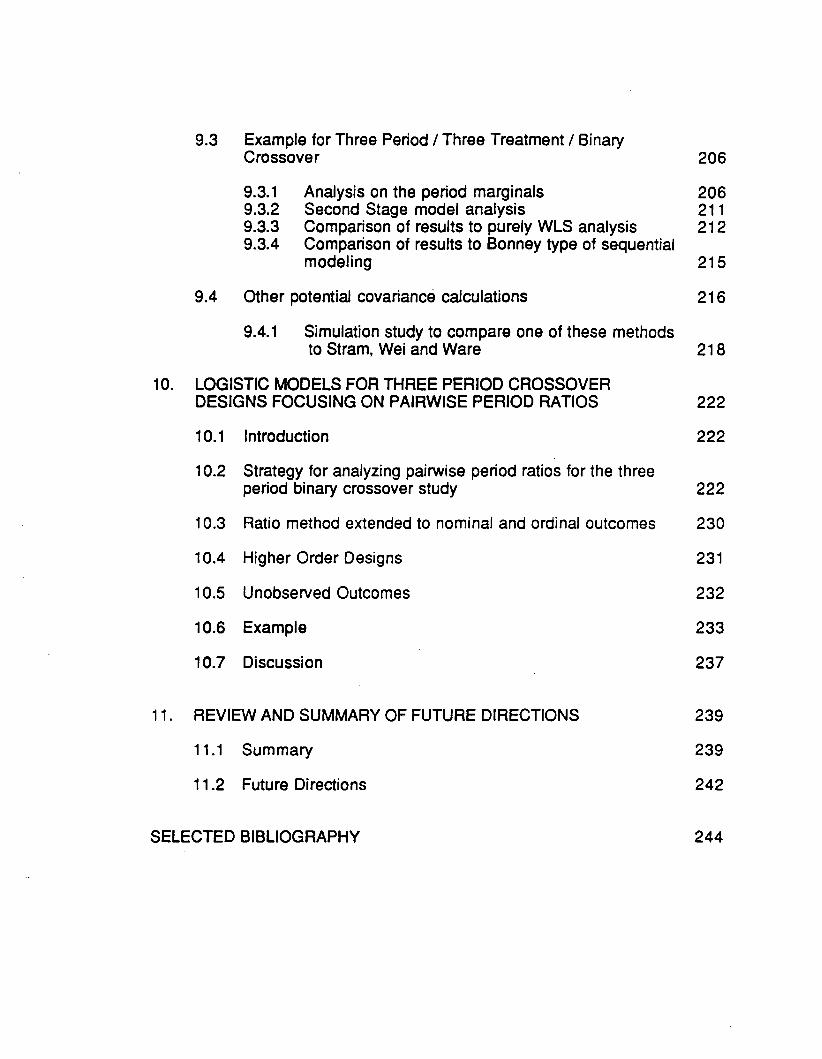
9.3 Example for Three Period / Three Treatment / BinaryCrossover 206

9.3.1 Analysis on the period marginals 2069.3.2 Second Stage model analysis 2119.3.3 Comparison of results to purely WLS analysis 2129.3.4 Comparison of results to Bonney type of sequential

modeling 215

9.4 Other potential covariance calculations 216

9.4.1 Simulation study to compare one of these methodsto Stram, Wei and Ware 218

10. LOGISTIC MODELS FOR THREE PERIOD CROSSOVERDESIGNS FOCUSING ON PAIRWISE PERIOD RATIOS 222


10.2 Strategy for analyzing pairwise period ratios for the threeperiod binary crossover study 222

10.3 Ratio method extended to nominal and ordinal outcomes 230

10.4 Higher Order Designs 231

10.5 Unobserved Outcomes 232

10.6 Example 233

10.7 Discussion 237

11. REVIEW AND SUMMARY OF FUTURE DIRECTIONS 239

11.1 Summary 239

11.2 Future Directions 242

SELECTED BIBLIOGRAPHY 244

CHAPTER 1

REVIEW OF CROSSOVER DESIGNS AND

METHODS FOR THEIR ANALYSIS

1.1 Overview of Crossover pesigns

1.1.1 pefinitjon and objectives

Crossover designs (also referred to as change-over designs) are

experimental investigations where subjects are randomized to treatment

sequences, thus providing an instrumental assessment of treatment differences.

Each group of subjects receives the specified treatments in a different order.

These designs are applicable for treatments that promote a temporary rather

than permanent change and where the condition can be considered

reproducible within a given patient. Conditions such as asthma, angina,

headache or heartburn are common investigative themes for crossover trials.

Since subjects are observed at more than one time point, crossover studies

belong to the general class of multivisit studies which describe response status

over time or condition for a group of individuals. The characterizing feature of

this design is reflected in the structure of subjects randomly assigned to different

treatment sequences. Multivisit studies and crossover designs are special types

of longitudinal studies where responses can be broadly fol/owed over longer

periods of time, and both longitUdinal studies and multicondition studies belong

to the general class of repeated measures studies.

To consider the scope of crossover designs more fUlly, first note that the weI/

known two period, two treatment crossover design has by far received the most

attention. Here, SUbjects are randomized to two groups receiving the treatments

A and 8 in either the order A:8 or 8:A. Thus, two treatments are being compared

at each of two periods across the two sequence groups.

For example, patients are randomly assigned to receive an active treatment

(A) for the relief of heart burn in either period 1 or 2. For the other period, they

2

receive a placebo (treatment 8). Thus, the group A:8 receives their active

treatment in period 1 and placebo in period 2, both following a symptom

provoking meal. The outcome of interest is the measurement of relief from

heartburn.

Crossover designs can be much more general than the two period, two

treatment design for which so much attention has been directed, particularly for

the continuous outcome. The following sections will explore the breadth and

complexity common to crossover designs, while reViewing methods developed

to account for the uniqueness inherent in this design protocol.

1.1,2 Bange of designs and relevant hypotheses

The major defining elements of any crossover design are the number of

periods over which subject evaluations are made and the number of treatments

that the investigator wishes to compare. A practical crossover trial may involve

two to four periods to assess two to four treatments. Furthermore, subjects may

be further divided into strata for factors such as clinical center or gender, and

the role of continuous measures such as age may be of interest as covariables.

Another important consideration for analysis of the crossover design is whether

the observed outcome is a continuous or discrete measurement.

For crossover studies, one needs initially to focus on the hypotheses

addressed. Koch et al. (1977) and Koch et al. (1985) discuss hypotheses of

interest for many types of multivisit studies. The following objectives are

expressed in terms specific to the goals of a crossover trial. A treatment effect

indicates whether there is a difference in the treatments for the measured

response. For instance, does treatment A successfully prevent or diminish

heartburn relative to the placebo administration. This hypothesis is the major

focus of crossover designs.The period effect hypothesis addresses the issue of

response change across the time periods of treatment administration. A

carryover effect is directed at a potential interaction between the period and the

treatment effects, Le. treatment difference is larger in one period than the other,

For instance, the group receiving A:8 may still be experiencing a residual effect

treatment A while the administration of treatment 8 in period 2 is occurring. In a

mulitcenter study like this example, one could look at the period by clinic

3

interaction or the treatment by clinic interaction to see whether the response

changes across time periods differ for the clinics.

A useful extension of the two period protocol with two treatments has

additional sequences such as A:A and 8:8. These groups involve subjects

receiving the same treatments at both periods. This lends more power and

accessibility to estimation of effects, particularly with respect to carryover (see

Elswick and Uthoff (1989) ).

Also, with two periods, one could compare more than two treatments. For

example, two active treatments A and 8 could be compared to a placebo drug C

with appropriate combinations of the following sequences: A:8, A:C, 8:A, 8:C,

C:A, C:8, A:A, 8:8, C:C. While one still compares the effect of the first period vs

the second, there are three treatment comparisons of interest : whether

treamtent A performs better relative to treatment 8 or relative to treatment C, and

whether treatment 8 performs better relative to treatment C. Also, there are three

carryover comparisons to consider. The selection of sequences can be

motivated by the desire to produce more precise treatment estimates for certain

combinations of interest.

The scope of crossover designs can be further expanded to include additional

periods. Subjects can randomly be assigned to sequence protocols involving

two or more treatments where outcomes are observed across three or more

periods. Consider an example for a three period design where the following

three treatments are compared. Treatment A is a fuJI dose of a drug intended to

relieve heartburn, treatment 8 is half dose of the same drug and treatment C is a

placebo. In order to compare the effectiveness of this drug relative to placebo

and to assess the difference between the two dosages, the subjects may

receive the drugs in the order A:8:C, 8:C:A or C:A:8. These three groups are

sufficient to jUdge the significance of period, treatment and carryover effects.

Supplementing the protocol with the additional Latin square of sequences

A:C:8, C:8:A, and 8:A:C provides more power for estimation of carryover effects

and treatment effects adjusted for carryover effects. Also, with three period

designs, more than two or three treatments can be considered with attention

directed at which parameters are estimable with a particular analysis strategy.

4

Furthermore, any number 01 periods or treatments can be implemented in a

design with a variety 01 sequence groups chosen to best estimate the effects of

interest. Practically, clinicians rarely use a design with more than four periods.

Another noted advantage is that multi period designs with only two treatments

are helpful for assessing carryover effects when they are anticipated to be

substantial (Laska, et al. (1983) ).

The implementation of any of these crossover designs at multiple clinical

locations -extends the scope of the problem to include center effects. Of further

interest may be the center by treatment interaction. Background characteristics

such as gender or age can be taken into account for their potential interactions

with treatment or period effects. Also, period dependent covariates such as

baseline stmptoms can be considered.

Another extension of crossover designs is their multiple use for the same

subject at two or more sites or two or more times. An example is a dermatology

study for the relief of a skin condition; the right arm receives one treatment

sequence for two or three forearm sites and the left arm receives another

treatment sequence. Thus, each patient receives two treatment sequences

according to a specified structure.

1.2 Review of methods for Two Period. Two Treatment. Two SeQuence

Crossover Designs

Much of the work that has been done for the crossover design for both the

continuous score and the categorical score is for the two period, two treatment,

two sequence design. Section 1.2.1 will develop the standard two period model

for the continuous data. Section 1.2.2 provides a review of existing methods for

categorical outcomes. The focus of this research will be on the binary, nominal

and ordinal responses.

The classical two period two treatment crossover study has been utilized in

many experimental situations to compare two treatments where subjects are

randomly allocated to one of two sequence groups. One sequence group is A:B,

denoting treatment A is administered in the first period, followed by treatment B

in the second period with an appropriate washout period in between. The

5

second sequence group, denoted by B:A, receives the treatments in the

opposite order.

Because the subject serves as their own control, a number of advantages are

evident. The treatment comparison, a major focus of concern, is made relative to

within subject variability. Fewer subjects are required to have appropriate

statistical power for treatment comparisons. Thus, crossover studies provide a

more sensitive and powerful test than other study designs utilizing among

(rather than within) subject variability. The management of this subject effect is a

crucial research issue determining the approach of the methodology. The

crossover design is particUlarly applicable when the treatments affect a

temporary rather than permanent change in the condition under observation.

Thus, investigations concerned with the relief of a medical condition (e.g.,

headaches, heartburn following a symptom-provoking meal, etc.) lend

themselves well to crossover designs. In addition to detecting treatment

differences, investigation will also focus on possible period effects and

evaluation of whether a carryover effect has occurred. A significant treatment by

period interaction is indicative of a carryover effect of treatment from the first

period to the second period. In the presence of this effect, caution should be

directed at interpreting estimates of treatment effects.

1.2.1 Literature review of methods for crossover designs with continuous

measures

Crossover designs probably were used first in agricultural studies where plots

of land received alternating treatment applications during the mid 1850's.

During the 1930's, researchers began to consider carryover effects different

from treatment effects. Simpson and Yates employed crossover trials comparing

diets in children. Animal husbandry studies are another area in the background

of early use of crossover studies, as well as biological assay studies. More

detailed information on these is provided by Jones and Kenward (1989) and

Bishop and Jones (1984).

More recently, focusing on medical related studies, a variety of methods exist

for handling the continuous outcome. Repeated measures analysis of variance

techniques as well as other parametric methods are available. The work by

6

Grizzle (1965) has received significant attention. He proposes a method for

considering the significance of the carryover effect before assessing the

treatment effect for the two period and two treatment trial. He asserts that this is

necessary because treatment effects are biased when an unequal carryover

effects exists.

To consider in more detail a standard parametric model proposed by Grizzle,allow the continuous outcome to be Yijk for the i-th sequence group, j-th period

and the k-th person. The model is

Yijk = Jlij + <Xik + eijkwhere aik is the k-th subject effect and the eijk are the random error terms of the

model. When the aik are random subject effects with null means, the Ilij have

expected value structure as follows:

Sequence GroupA:BB:A

Period 1

Il + 1t1 + t1

Il + 1t1 + 't2

Period 2

Il + 1t2 + 't2 + A.1

Il + 1t2 + 't1 + A.2

where the period, treatment and carryover effects are denoted respectively by 1t,

't and A..

This structure also applies to sample mea~s Yij. = L Yijk / nj when the aik are

viewed as fixed effects with the restriction L <Xik =O. In the random effects case

the aik are assumed to have mean 0 and variance CJa2. Thus, CJa2 is the

covariance of responses from two different periods for the same subject. Thisaccounts for the correlation inherit in the crossover design. The error terms eijk

are also assumed to have mean zero and varaince CJe2. Thus, the variance of

the subject's response is CJa2 + CJe2. Responses from two different subjects are

considered independent.

A test of the carryover effect is performed with a two sample ttest relative to thesums of the subjects responses, Le. Yi1 k + Yi2k. For this test, normal

distributions are assumed in small samples. Given no significant carryovereffect (Le. A.1 =A.2) , treatment effects are assessed with a two sample ttest on the

difference in responses for two periods, Le. Yi1 k - Yi2k. This within subject

difference allows for the cancellation of subject effects, so the model is

7

applicable whether the subject effects are fixed or random and allows forreduced variance involving only ae2. If there exists a significant carryover

difference, Grizzle (1965) has proposed an assessment of treatments from

period one data only.

Also, assuming equal carryover effects, another way to proceed with this

analysis is to do an analysis of varaince with subject, treatment and period

effects.

Nonparametric methods can be useful when assumptions of normal

distributions are not met (see Koch (1972) ). For example, where ttests were

previously discussed, Wilcoxon tests would now be appropriate. Elswick and

Uthoff (1989) present a nonparametric approach for the two treatment, two

period design with the four sequence A:A, A:8, 8:A and 8:8. He notes that this

design is optimal in the presence of carryover effect. The methods he considers

are analogous to the randomized complete block analysis of variance with

treatment. period, carryover and sequence effects.

1.2.2 Reyiew of methods for crossover designs with the categorical outcome

For categorical outcomes, most of the available methods have been primarily

focused on binary outcomes. Gauss (1986) provides an excellent brief overview

of methods for the crossover design with binary responses. The methods

presented below deal exclusively with the two period, two treatment design

(known as the classic 2 x 2 study). For this case, let the two sequences groups

be A:8 and 8:A where the first group receives treatment A then treatment 8 in

that order. Group 8:A receives them in the opposite order. The joint outcomepossibilities for (Yi1 k, Yi2k) are (00), (10), (01) and (11) where the binary

indicator Yijk corresponds to the k-th person, i-th sequence group and j-th

period.

McNemar (1947) was probably one of the first persons to consider the

treatment effect in this setting of the 2 x 2 design. He used only the discordant

outcomes (01) and (10) relative to the two treatments and proposed a test for

these pairs from the pooled sequence groups through a binomial distribution

with the probability of one-half. He assumes no other effects such as subject

8

effects, period effects or carryover. When these assumptions hold, his method

has been shown to be optimal as compared to Gart's method (1969).

The methods of Gart (1969) (also referred to as the Mainland-Gart test) will be

presented in full detail in Chapter 3. Briefly, Gart also considers the discordant

joint outcomes. He assumes no significant carryover effects and that conditional

independence holds (Le., within any subject, responses for the two periods are

independent). His test for treatment given the period effect is equivalent to

Fisher's Exact test for the two by two table in which the rows are the two

sequences and the columns are the (01) and (10) discordant outcomes in

McNemar's test.. Le (1984) and Le and Cary (1984) extend the Gart model for

the 2 x 2 design to the nominal and ordinal outcome. Their work also makes

use of discordant outcomes and will be discussed further in Chapter 3.

Disadvantages of these methods are that they do not allow for carryover effects

or missing data. Le and Gomez-Marin (1984) provide the maximum likelihood

estimates and standard errors for Gart's logistic model. These results were

suggested as useful with multi-eenter clinical trials and are based on the

weighted average of effects across the centers. The appropriate weights are the

inverses of the computed variances.

Prescott (1981) also develops a method for the 2 x 2 design with the binary

outcome, again assuming no significant carryover effect. He considers only

period, treatment and fixed subject effects. He presents a randomized test (not a

model based test), where he creates a difference measure d=1, 0 and -1 for

joint outcomes (10), (00) and (11) combined and (01), respectively. Then he

performs a trend test for the 2 (sequence) by 3 (score) table. Although this is a

distribution free test for treatment, he provides the large sample test for

treatment effect based on the normal distribution. He asserts that one-half of the

distance between the average d score for the A:B group minus the average d

score for the B:A group is an estimate of the average treatment effect. Prescott

also provides a simulation study to compare McNemar's test vs Gart's test vs his

strategy. He asserts that his test is optimal, and between Gart's and McNemar's

test, McNemar's is superior when there are equal numbers of patients in each

sequence group and/or when there is no period effect.

9

A similar nonparametric test was proposed by Armitage and Hill (1982) and

Koch (1983). They present a randomization test for carryover effect which

focuses on a sum score assigned as values 0,1 and 2 for groups (00), (10) and

(01) combined and (11), respectively.

Farewell (1985) also_ has a method for the 2 x 2 trial, where he extends the

logistic model to the trivariate response s=O, 1 and 2 for joint outcomes (10),

(00) and (11) combined, and (01), respectively. He also assumes no carryover

effects and that treatments are comparable across sequence groups. He

provides a global test of fit as well as an odds ratio interpretation.

In order to address the issue of carryover effects, both Cox and Plackett (1980)

and Hills and Armitage (1979) provide frameworks. Cox and Plackett (1980)

present two models. The first is a simple contingency table approach where the

empirical data proportions provide estimates for the marginal probabilities.

Then there are 4 equations in 4 unknowns to solve for the parameters. This test

requires that the odds ratios are homogeneous across sequences for the effects

to be interpretable from the marginal probabilities. Their second method is a

random effects model for a probit analysis. However, this approach requires a

lot of distributional assumptions and extensive computing. Furthermore, the

likelihood ratio tests are very complex.

Hills and Armitage (1979) consider the 2 x 2 design for the ordinal response,

and use a model with period, treatment and carryover effects. For the binary

response, their test for the carryover effect is based on the frequency of the (00)

and (11) concordant pairs. They test for the treatment by period interaction with

a test for independence on the 2 x 2 table where the two rows are the sequence

groups and the two columns are the responses (00) and (11).

Fidler (1984) also looks at the 2 x 2 design for the binary response. With a

mixed model approach, a bivariate logistic model allows for modeling of period,

treatment, carryover and association effects to the joint probabilities. These

association effects measure the dependency between the observations across

the periods. Their method is very similar to that of Jones and Kenward (1988) to

be discussed next. Jones and Kenward offer criticism that Fidler's parameters

are difficult to interpret, and that there is some confusion between the

association and carryover effects. They say that these two effects cannot be

10

separated out and thus, Fidler's strategy cannot be extended to more

complicated designs.

A chapter of this research will address the noteworthy methods of Jones and

Kenward (1988 and 1989). They fully develop their model for the categorical

outcomes (both bin~ry and ordinal), for two periods and two treatment

administrations. Section 1.3.2 will consider this model for multi period designs.

They also use logistic or log-linear regression to model the joint probabilities.

Disadvantages of their log-linear model as well as problems with its application

to the examples they provide in their textbook will be discussed in Chapter 8.

Major differences of their method relative to the one investigated in this

research is the management of subject effects and the definition of parameters

with respect to joint rather that marginal probabilities. A further limitation of their

method is that parameter interpretation depends to some extent on the number

of periods in the design protocol and hence can become complicated in

situations with missing data.

Another strategy available to the researcher could be the use of weighted

least squares analysis. Zimmermann and Rahlfs (1980) apply WLS to the linear

probabilities to estimate a reference mean, period, treatment and carryover

effects. For the 2 x 2 design, the period and carryover effects are partly

confounded, and this limits the interpretation and range of validity of

parameters. This method can be easily extended to more than two periods and

more than two treatments.

Koch et al (1983) also employ weighted least squares analysis to the

crossover design in order to assess period, treatment and carryover effects.

They also indicate how to incorporate covariate groupings into the analysis.

This paper also provides a nonparametric analysis with a particular emphasis

on assessing carryover effects.

1.3 Reyiew of methods for muHt period or multi treatment designs

The crossover design need not be limited to the classic 2 x 2 trial. Multi period

designs of more than two periods are feasible as are studies combining two or

more treatments in any variety of sequences. As the number of periods,

11

treatments and or sequences increases, the likelihood of incomplete data arises

and analysis needs to account for this concern.

1.3.1 Continuous Outcomes

For the multi period design, one can extend the model of Grizzle (1965) to

include effects for period, treatment and carryover (Koch, et al 1988). The same

issue of correlation from period visit to visit exists, but simple ttests are no longer

available. An analysis of variance extension can be appropriate. With this basic

additive error model, one assumes that the variance of all the periods are equal

and the covariance between pairs of periods are equal. From this model, one

can test period, treatment and carryover effects, as well as potentially

meaningful interactions of covariates with treatment. Assumptions for this

relative to subject and error effects are similar with respect to normality with the

appropriate variance structure. With a within subject analysis, the subject effects

are eliminated, regardless of the assumptions attributed to them. Thus, the

applicable varaince is the within subject varaince. Also note, with a within

subject structure, it is not feasible ot look at a covariate main effect.

When the assumptions of this model do not hold, a model with more general

covariance structure is potentially needed. Although its discussion is beyond

the scope of this work, its counterparts for categorical outcomes will be

addressed.

Other parametric techniques for the three period and two treatment design

have been described by Hafner, Koch and Canada (1988). One method among

others is to model the within subject linear function to estimate effects for each

individual. Then these parameters are compared with a standard univariate

analysis of variance.

1,3.2 Categorical outcomes

Particulary for the categorical outcome, little work has been done for multi

period designs. Most of the work has centered on the classic 2 x 2 design. Even

for the simplest dichotomous case, section 1.3.2 showed a variety of competing

methods. Almost no work exists to handle the broader scope of crossovers as

presented in the design structures section 1.1, particulary when missing data

12

may be present. The following section briefly summarize the methods that do

exist.

The available methods for analyzing categorical outcomes from a multi period

design are very limited. Weighted least squares methods are in principle

applicable here through straightforward extensions to the methods presented in

section 2.4.2. However, multi period crossover designs rarely have a large

enough sample size to support this general method. A study with at least 20

subjects per sequence group is often impractical, particulary as more

combinations of treatments are compared.

Jones and Kenward (1988) in their paper in Statistics in Medicine present an

example for a three period, three treatment design. More details of their

extension beyond the classic 2 x 2 design will be presented in Chapter 8. While

their model generally applies to any multi period design, it becomes awkward to

use because of the proliferation of parameters tied to the joint period

distribution. As also discussed in Chapter 8, Jones and Kenward's

management of zero cells in contingency tables for data summarization

presents difficulties that can become extensive since more periods and/or

treatments usually imply more cells of data with zero counts.

1.4 Data structure and Questions for analysis

1.4.1 Data structure

A distinguishing component of crossover designs not evident in cross

sectional studies is association or correlation among the responses.

Measurements from the same subject for two different periods are more likely to

be similar than if they come from different sUbjects. Also, adjacent periods may

be more related than periods farther apart in time. Thus, it may not always be

appropriate to make the assumption of homogeneous variances and

covariances as often done for multiperiod crossover studies with continuous

data. Furthermore, categorical data cannot be expected to follow simple

patterns of correlation. The pattern of correlation within a subject and for

adjacent periods influences the structure of the covariance matrix associated

with the estimated parameters. Accounting for this correlation presents a

problem that will be addressed in methods for this research.

13

Another consideration to evaluate the data structure of crossover studies is

the measurement scale. The focus of this research will be for the categorical

response. The discrete outcome can be observed as dichotomous, nominal,

ordinal, discrete enumeration, or grouped along a continuum. Continuous

outcomes can also be measured in crossover trials. In addition, the types of

explanatory variables can be categorical or continuous. Here, they are mostly

considered categorical so that the number of subpopulations is fixed. This is

needed for many of the methods of interest in this research.

One important reason to use crossover studies is to increase the precision in

judging differences for factors observed within subjects such as treatments in

clinical trials. Because repeated observations are made on one subject across

multiple time points, a reduction in individual variation is achievable for

changes over time. Another objective of multivisit studies is examination of the

relationships of a person's response to time factors and other characteristics of

the subpopulations to which they belong. Cook and Ware (1983) provide an

excellent discussion of comparing advantages and objectives of longitudinal or

multivisit studies versus cross-sectional studies· with respect to design issues of

precision, cohort effect and missing data. They also address sources of error

variability and suggest strategies to improve the integrity of all aspects of data

observation and collection.

In addition to handling the full scope of designs available to the crossover

study, the research of this investigation will deal with the analysis of categorical

response measures for the crossover study involving multiple periods. These

periods of treatment administration have a fixed nature in that they occur at

predetermined times relative to protocol specification. Subjects can be cross

classified based on categorical explanatory variables, where change-over

structures applied at each of several clinical sites will make the clinic factor a

covariate of particular interest.

1.4.2 Releyant analysis issues

Another issue relevant to the data structure is that of missing data. This data

can be either missing by design or missing at random. Many statistical methods

14

deal with this problem by assuming that missing data occurs at random from

non-response or deleted incorrect response or that due to cost or study

emphasis, augmented data is obtained only on a sample of subsets. This can

be clearly seen with an example of a 3 period design. Data missing at random·

can occur when a patient doesn't show up for one or more of the scheduled

visits. Data missing by design could occur if due to budget or logistic

considerations, the patients were selected to randomly miss one of the periods

resulting in only 2 of 3 periods recorded. Related to this issue is that of sample

size and the number of factors considered. As these numbers increase, the

likelihood of missing data increases as well as computational difficulty. Thesample size ni in each subpopulation as well as the number of conditions

impact significantly on the methodology used.

Because each subject serves as their own control, the reduced within subject

variability allows for a more efficient judgment of treatment effects. Since any

one subject provides information on all of the treatments, relative to the parallel

groups study, the same subjects provide better statistical power, precision and

lower cost.

Methods designed to analyze the crossover study have as their primary focus

the comparison of treatments. They also must address the period effect. While

the investigator hopes to design a study where there is appropriate washout

time before the next treatment is administered, modeling of potential carryover

effects must still be considered. This reflects a period by treatment interaction.

One major issue determining the structure and focus of analysis is how the

SUbject effects are treated. Since one subject is observed for two or more

periods, any analysis must deal with the effect attribute to this subjects variation

regardless of any other effects such as treatment or period.

Subject effects may be viewed as random or fixed effects. Random effects

models have been discussed in great generality in a variety of contexts (see Gill

(1978) ), and so their principles are extendable to crossover studies when the

subject effects are random. When subject effects are considered fixed, there are

two appropriate cases, depending on whether certain restrictions hold. The

restriction that the average of the fixed subject effects in each sequence group

is zero is often supported by random assignment of subjects to sequence

15

groups. Depending on the type of function one wishes to analyze, different

structure of analysis with respect to the subject effect may be appropriate.

When the comparison across periods focuses on difference or ratio measures,

then one has an intrasubject analysis for either the continuous or categorical

outcome. This structure is applicable regardless of whether subject effects are

considered fixed or random because the subject effects are canceled out.

Gart's method for categorical data and the extensions presented in this work fall

into this category. In the standard two period and two treatment design, this

analysis presumes no carryover effect.

An intersubject analysis is appropriate when applied to a sum or to the period

one responses. The sum is often a more appealing response because it is

orthogonal to the difference measure. This type of analysis allows assessment

of carryover effect and treatment effect given a carryover effect in a two period

study. However, for multiperiod designs the role of this information is not as

clear since treatment, period and carryover effects are estimable within

subjects.

When both intra and inter subject information are used, one has a combined

analysis. For example, it can be applied to within subject sums and differences

for a two period design. Grizzle's (1965) work for continuous data is an example

of this. More specific details of this model are presented in the following

sections. The weighted least squares analysis, Jones and Kenward method

(1989) and Stram, Wei and Ware's (1988) method also fall into this class of

structures for the categorical outcome.

When the su~ject effects are considered random, any of the proceeding types

of analysis may be implemented. For fixed subject effects with the restriction

preViously discussed, intrasubject analysis is feasible. The inter-subject and

combined analyses are applicable but awkward. Without these restrictions and

with fixed subjects, the intersubject analysis cannot be used to estimate model

parameters because of confounding with subject effects. Thus only the

intrasubject analysis can be applied. The intersubject and combined analysis

cannot be applied.

For the continuous outcome with more complex, higher order designs, the

typically applied analysis is the intrasubject analysis. For the categorical

16

outcome, the Gart (1969) type model with the extensions proposed to more

complicated designs has the advantage of being consistent with the continuous

outcome strategies as it involves an intrasubject analysis.

A relative concern of this extension that needs to be dealt with is what

happens when the assumption of conditional independence, inherent in

intrasubject analysis, does not apply. Incorporation of association parameters

and how they impact the covariance structure will be looked at. This

corresponds to the more general linear models analysis, for continuous data

where a more general covariance structure is needed.

1.5 Overview of research

Most of the strategies for analysis of categorical data from the crossover

design are limited in focus to the two period, two treatment two sequence trial

for the binary response. There is a need to have methods that allow for a

response to be nominal or ordinal and for a general specification or two or more

periods and two or more treatments. Furthermore, many methods assume

models that only incorporate period and treatment effects. Strategies should

also assess the carryover effect and further allow for the dependency that

possibly exists between the measurements for the same subject across the

periods. Also, the strategies that exist are not readily applicable when there is

missing data. This is needed particularly as the number of periods increases.

The research here addresses each of these issues. Chapter 2 first reviews

categorical d~ta methods in general and then those methods more specifically

designed for crossover studies. It is necessary to relate the techniques of

maximum likelihood and weighted least squares, as they contribute to the

strategies applied to the crossover design.

Chapter 3 explores the model proposed by Gart (1969) and Le (1984).

Motivated by this model for the 2 x 2 case, some refinements are suggested.

Also this method is extended to other two period designs comparing two

treatments for both the binary and ordinal responses. Chapter 4 presents other

two period designs where there are three treatments applied in the sequences.

17

Chapter 5 considers the three period design for the binary and categorical

responses. This chapter further assesses the contribution of association or

dependency parameters to the model.

Chapter 6 deals with for the four period design. Embedded in this chapter is

the theory for the log-linear model with a multinomial distribution with varying

length response vectors. Furthermore, this chapter considers the general

structure needed to capture any design matrix for the extended Gart model for

any crossover design.

Chapter 7 addresses the issue of missing data. This will be motivated by a

discussion for the general three period design with a binary response, but

applies to all crossover designs.

While Jones and Kenward (1989) do present a method that addresses most

of these issues, their techniques have other disadvantages. Chapter 8 will focus

on their method. In particular, it becomes more difficult to model joint

probabilities as the number of periods increases. Also, their method defines the

parameters from the joint probabilities rather that from the marginals, as is done

in the proposed methods. Furthermore, their interpretation of parameters

changes as a different number of periods is a priori considered. This presents a

problem with strategies where one might wish to model subsets of the periods

within a large crossover design. The Jones and Kenward method does not

allow for missing data.

Chapter 9 overviews Stram, Wei and Ware's method for multivisit studies. The

goal of this chapter is to expand their methods to encompass the crossover

design by applying it to the first order period marginals. A discussion of potential

modifications to their covariance calculation is presented.

Chapter 10 presents a pairwise period ratio method focusing on ratios from

pairwise combinations of periods. Because these ratios are correlated, a

weighted least squares analysis will be used for covariance matrix estimation.

Chapter 11 concludes with a summary of the work and directions for future

research.

18

CHAPTER 2

OVERVIEW OF CATEGORICAL DATA METHODSAND OUTLINE OF RESEARCH

2.1 General Approaches to Categorical Data

Before looking at categorical data analysis strategies for crossover designs, it

is first necessary to understand the methods employed for general types of data

structure. Categorical data analysis has a scope which includes any data with a

response measure that is categorical. Commonly used methods are based on

randomization or on model fitting.

2,2 Randomization methods

Methods based on randomization principles involve minimal assumptions. In

particular, difficulties due to sampling issues are not of direct concern because

the subjects are not assumed to be selected from some large target population,

Thus, one limitation of this method is that inference is restricted to the actual

subjects who provide data. Rather than assuming random selection of SUbjects

for the underlying probability distribution as done in modeling methods, this

method is based on randomly allocated distributions for the response. Through

this, a structure to allow hypothesis testing is induced. Thus, another drawback

is that these methods are geared towards hypothesis testing and do not

generalize as with estimates from model fitting.

Examples of randomization methods include well-known nonparametric

methods and contingency table methods. Common tests are the Kruskal and

Wallis (1953) one-way rank analysis of variance criterion, the Friedman (1937)

two-way rank analysis of variance, the Spearman rank correlation test statistic,

Fisher's (1935) exact test for 2 x 2 tables, and Mantel-Haenszel (1959) statistic

for sets of 2 x 2 tables. Further discussion is available in Koch, Gillings, and

Stokes (1980) and Koch et al. (1985).

19

The focus of this research is on methods describing relationships; thus,

randomization methods are not of primary interest. Alternatively, attention is

directed at maximum likelihood and weighted least squares strategies for fitting

models. Maximum likelihood methods are applied to individual responses

where weighted least squares methods describe variation among aggregates of

subjects through sets of functions with estimable covariance structures.

2,3 Maximym likelihood methods for log-linear models

Maximum likelihood methods are predominantly used to fit log-linear models

to a cross-classification of variables.This method assumes that the likelihood

function for the data is known, for example either Poisson or product

multinomial cases. Estimates are then generated for the parameters in models

describing the variation among log-linear functions. An advantage of this

technique over the weighted least squares method is that a smaller sample size

is required for justification of asymptotic properties for some classes of models.

This strategy as presented by Koch et al. (1985) involves fitting the log-linearmodel based on the vector 1t of product multinomial probabilities. Based on this...multinomial framework, where the frequencies Yij correspond to the counts in

the i-th of s subpopulations and the j-th of the r response outcomes, the

likelihood function is

n II YilPr{y} = [ no,. ! ( 7t"

IJi.1 j =1

/ y.. ! ) ]IJ

(2.3.1 )The vector y is the compound vector of the sr frequencies and nj* represent the-total counts in the i-th subpopulation. A further assumption is that the {1tij} satisfy

the natural constraints

! 7t oo = 1o 1 'JJ=

for i = 1, 2,. . . s.

(2.3.2)

20

The log-linear model is

F(x) = A [log x] = A X ~ ...., -.i <tW N"'''''-

(2.3.3)In this specification, ~ is the (s(r-1) x sr) orthocomplement matrix to the matrix

specifying the natural restrictions in (1.2.2) and ~ is the known (sr x t) design

matrix of full rank t <= s(r-1) and linear independence from (1.2.2). With this

parameterization there are ~ distinct subpopulations, r levels to the response

outcome, and t parameters to be estimated. The log-linear model can also be

expressed in direct exponential form

5 = 9,,-1 [exp (~ ~) ] ."" (2.3.4)

where, in order to satisfy the restriction in 1.2.2, " is the vector of appropriate...denominators which standardizes ( exp(X~)). Thus,

" = [ 1r 1r' ® I] [exp (X ~)],....".,.,J IOJ 'V".,J

(2.3.5)

where 1r' represents a vector of r 1's of the appropriate dimension and I is theN ~

(s X s) identity matrix.The common notation, 9:}"1, refers to the diagonal matrix

consisting of the elements of the reciprocal of " on the diagonal, and ® denotes..Kronecker product (by which the matrix on the left multiplies each element of the

matrix on the right).

Another way to look at the log-linear model is to consider that for the r levels

of response, r-1 logits are analyzed where the k-th logit is

logit (8ik) = loge {xik / xir} .

(2.3.6)The logit is the logarithm of the odds of proportion of one response relative to

another. Thus one type of log-linear model can be specified through each logit

as

21

logit ( 8ik) = <lk + xi' ~k .

(2.3.7)

There are separate intercepts and regression parameters for each logit.

Comparing between two subpopulations involves r-1 components, and thus no

underlying structure in response.

For the log-linear model, substituting equation 1.2.4 in for 1.2.1 yields thelikelihood <1>( ~) that can be used in equation 1.2.7 to obtain the maximum...likelihood estimate of ~.

N

[a log <I> I • ]a~ ~=~ = at- --

(2.3.8)

Differentiating this matrix equation yields the compact expression for the

equations specifying maximum likelihood estimates.

"X'J,1=X'y

(2.3.9)where J.1 is the vector of estimated expected frequencies assuming the log-

N

linear model. An explicit solution for ~ is not available so Newton-Raphson isN

the usual numerical algorithm. The estimated ~ is asymptotically equivalent to,..the weighted least squares estimate b in (1.2.23) where (1.2.3) is the log-linear...model.

'"Based on results of Imrey et al. (1981) and assuming the model, (~-~) has,.. -

an approximate multivariate normal distribution with covariance matrix as

follows:

-1

{ ! n.• X.' (0 - 1t. 1t .' ) X. };=1 I _ I _ 1t i_' _ I _ I

22

(2.3.10)

Goodness of fit for the log-linear model can be evaluated with either of the

following statistics both of which have asymptotic chi-square distributions with

(s(r-1) - t) degrees of freedom. The Wilk's log-likelihood ratio statistic is

"YI'J' log (y .. / ~ .. )

IJ IJ

(2.3.11)

and the Pearson chi-square statistic is

i= 1 j = 1

" 2(Yij - Il ij )

"/ ~ ..

IJ

(2.3.12)

2.3.1 Maximum likelihood methods for ordinal data

When the response outcome can be considered ordinal rather than just

nominal, then a more specific type of model structure can be employed.

Ordinality of response implies an underlying scale structure to the response. For

instance, the categories none, slight, moderate, and severe reflect an

underlying increasing severity level.

One way to take this structure into account is with an equal adjacent odds

ratio model. This model is also a log-linear model with general specification

1t.. =IJ

,

exp (a. + (r-j) x . p )J _ I _

1 + !: exp ( a, +' (r-j) x',, 1 J - IJ=

p )fa r j = 1, 2, . , . r-1

1t.Ir

= 1 -!1t ... IJJ=l

23

(2.3.14)

Thus, for the k-th outcome response,

6ik

=1t

ik =1t.

I r

exp ( (lk + (r-k) ~ ik' ~ )

(2.3.15)The logit can then be expressed as :

logit ( aik) = (lk + (r-k) ~ ik ' ~ for j = 1, 2, ... r-1

(2.3.16)

This model gets its name because one assumes equality of the odds ratios

involving adjacent response categories. Since the odds ratio measures

difference or distance with respect to distributions of outcomes, this assumption

states that for any two subpopulations, the odds ratio of response for the first

response versus the second response is equal to the odds ratio of the second

versus third response. From this model structure and assumption, the

relationship exists for the i-th and i'-th subpopulations:

1t .. 1t.,log { II I r }

e 1t. 1t. ,.Ir I J

.= (r-j) (x. - x.J ~

- I _ I _

= logit ( a.. ) - logit ( a". )IJ I J

(2.3.17)

One limitation to this model is that computation for it is not convenient for

continuous predictors. Another is that the ordinal response categories must be

fixed and prespecified. Also, they must be non-poolable; since pooling would

24

contradict the model because of the different specification to the logits.

McCullagh (1980) and Imrey st al (1982) provide further discussion of this.

Another model that accounts for the ordinality of the response categories, but

does not have the advantage of being part of the general class of log-linear

models, is the proportional odds model with the general form

~ , -1L 1t .. , = {1 + exp (-a. - x. J3)} .

j' :II j + 1 I) J "J I ...

(2.3.18)

This specification looks at a parallel set of logistic models. The k

th cumulative logit can be shown as

logit (~ik)

,

a + x 13.k ...)....,

(2.3.19)

This model has the advantages that categories can be pooled as if along an

underlying continuum and that both continuous and categorical predictors can

be used. The assumption made for this model is that for different

subpopulations, the difference between cumulative logits is independent of the

response category. This implies that the odds ratio for the patient in the i-th

group versus the i'-th group have the same value

t "ih (1 - t "i'h )h=1 h=1 = exp { (x. - X j' ) 13 } .

- I _ ,..J

(2.3.20)

In looking at the r-1 partitions of the r categories into less favorable versus

favorable response subsets, exp(J3) is the multiplier vector associated with the.-J

25

odds of more favorable versus less favorable per response change in

subpopulations.

This model and parameter estimation are discussed further by McCullagh

(1980). For both the equal adjacent odds and proportional odds models,

maximum likelihood methods will provide estimates for parameters andcovariance matrices; goodness of fit tests are based on counterparts to QL and

Q p in (2.3.11) and (2.3.12).

An alternate way to assess goodness of fit for the proportional odds model is

to use maximum likelihood to fit separate logistic models for each of the binary

more favorable / less favorable pairs. For example, for the data with four ordinal

categories A, B, C, and 0, fit three separate models for the pairs A vs. BCD, AS

vs. CD, and ABC vs. D. Then the parameters are compared across the models

to assess appropriateness of the proportional odds assumption. The goodness

of fit of the proportional odds model is supported when these parameters show

similarity across the different models. The method of Stram, Wei and Ware, to

be addressed in this research is an extension of this idea; separate logistic

models are applied to the individual time points in a longitudinal study as

suggested here for the separate logits and then parameters are compared over

time.

2.3,2 Seyeral Models of Application

Several strategies will be briefly presented here, all of which make use of log

linear models with maximum likelihood techniques. Each of these methods can

specifically address the crossover design.

Bonney (1987) proposes a logistic method for binary dependent outcomes,

His approach is a successive strategy for the conditional probability of one

response conditioned on all previous visit responses. Thus, the dependent

problem is transformed to independent univariate logistic regressions. One

disadvantage of this strategy is that it is difficult to interpret parameters or

reconcile the effects between the various models. Missing data can only be

incorporated if all missing data reflects the successive dropout of patients. For

the crossover study, the models apply successively to period one, period two

given period one, and so forth.

UtiliZing a weighted least squares approach, Koch et al. (1977) have proposed

a method looking at the marginal probabilities within a repeated measures

26

framework. This method will later be reviewed in more detail and can be

applied to the crossover study. Stram, Wei, and Ware (1988) also look at the

marginal probabilities to maximize the log likelihood function at each time point

for a multivisit study. They make the assumption that either the proportional

odds model or the proportional hazards model is applicable. Their method

proceeds in two stages, where at the first stage separate maximum likelihood

estimates are generated for each time point. The second step involves mUltiple

hypothesis testing procedures to assess variation across the multiple visits.

Their second stage assessments could be improved upon by a weighted least

squares analysis. This would aid in testing parameters across time and allow for

further model reduction. In addition to estimating these parameters at each visit,

they propose an estimate of the covariance matrix for them which relies on a

combination of both model based estimates of the marginal probabilities as well

as data specific estimates based on proportions. This formulation provides a

viable estimate for the covariance between estimates for any two of the multiple

visits. However, it should be noted that for anyone of the visits, the formula for

the variance differs from the one that is used in maximum likelihood logistic

regression based on a first principles approach with respect to the moments of

the distribution. This difference is potentially magnified in the situation with case

record data. The advantages of this strategy are that ordinal outcomes can be

used, missing data can be incorporated with some success, and time

dependent covariates are allowed. A further disadvantage of their method is

that they do not model all of the multivisit data together. Chapter 9 presents how

this strategy can be extended to the crossover design by modeling each of the

periods separately. How to accomodate the correlation across the periods by a

combined analysis wil be further discussed.

Zeger and Liang (1986) have proposed a general quasi-likelihood approach

that can be applied to both continuous and discrete data. This approach is

appropriate when the regression equation for the marginal expectation is of

main interest rather than the conditional expectation as utilized in more

traditional likelihood methods. All estimates across all visits are modeled

simultaneously and arrived at with iteratively reweighted least squares. This

strategy can be viewed as a refinement to Stram, Wei and Ware's approach

considering that the two covariance formulations are similar. The Liang and

Zeger covariance matrix has the same pivotal quantity with the additional

27

correlation assumption as an added component. Furthermore, the correlation

matrix must be considered a set of nuisance parameters since a working

correlation matrix must be initially specified which is not expected to be correct.

The goal is for the estimators to be consistent even when the correlation matrix

is incorrect.

Another strategy of Kenward and Jones (1989) applies a log-linear model to

the joint classification of responses across the periods. Again, maximum

likelihood techniques can be used to estimate the parameters relative to their

definition. Chapter 8 describes these details.

Conaway (1989) presents a conditional likelihood method for repeated

measurements. Based on the assumption that responses across the visits are

independent (local independence), he conditions on the sufficient statistics

which are the sums across the visits. This application applies to the longitudinal

study. The methods of this research will present a more general specification of

this idea motivated by the crossover design as well as a strategy to assess

goodness of fit and modify designs in the face of lack of fit of the model.

While all of these strategies allow for estimation of period, treatment and

carryover effects, they are defined from different frameworks. When the effects

are defined relative to the joint probabilities, they do not allow for a

straightforward interpretation for marginal or successive probabilities, and visa

versa. A simple structure for one defines a complicated structure for the others.

2,4 Weighted least sQuares methods

Another major model-based categorical technique involves weighted least

squares (WLS) as an analysis strategy for assessing variation among

proportions, functions of proportions, and measures of association. It is

especially appropriate in the case where a major assumption of usual least

squares, that of homogeneous variances, is not met. While WLS estimation

enables description of the variation among functions of the response

distribution with regard to the cross-classification into sUbpopulations, Wald chi

square statistics are used to assess the goodness of fit of the models.

The overview of this strategy will follow that presented by Grizzle, Starmer,

and Koch (1969) and Koch et al. (1985). The required components to initiate

this strategy is the vector of functions, F with dimension (u x 1 ), and its,..,

28

associated covariance matrix, 'if, which is nonsingular. Methods are then

employed to estimate parameters from the linear model

EACf} = ~~

(2.4.1 )

where X is the ( u X t ) design matrix of full rank t <= u. The unknown parameters'J

are shown in ~ which is a ( t X 1 ) vector. The expression EA { } represents theOJ

asymptotic expected value.

It will be assumed that the data are distributed as product multinomial (see

2.3.1) and this probability model will allow inference to a larger target

population. The data is laid out such that the independently selected samples is

s sUbpopulations are indexed from i = 1, 2, ..... s. These samples have been

obtained by a process equivalent in spirit to simple random sampling. The index

j = 1, 2, .... r corresponds to the level of the response profile within which the

subjects are classified, thus resulting in an s x r contingency table. The

sampling framework associated with the contingency table implies a product

multinomial distribution.Let Yij denote the frequency of the j-th response in the i-th subpopulation. Let

the vector y =(Y1 " Y2 " ... Ys ')' be the vector of s*r frequencies where Yi ' is"'V 1\,,... ,.... ".",

the vector of counts for the i-th subpopulation. Let ~ t = ( 1tt l, 1tt2, ..., 1ttp) , and

Pi = ( Pi1, Pi2, ... , Pir)' = (Yil ni*) be the vector of probabilities and sample....proportions, respectively, for the i-th population. Combining across all ssubpopulations, 1t = (1tl', 1t2', ... 1ts') , is the compound probability vector and

""'- A. _ ,.

P = (P1', P2', ..., Ps')' is the sample proportion vector. The 1tij must satisfy the--.. ... "'" ""-

constraint

j =1

! 1t ..IJ

= 1 for i=1, 2, ... s

(2.4.2)The Pij = Yij I nj are the unbiased estimators for 1tij, thus E(p) =~ and,..

29

V1 (1t 1 ) 0

..., rr

Var (p) = 0 ~ 2 (1t 2 )rr

.... V s (~ s )~

(2.4.3)

where the covariance for the i-th subpopulation is

v . (1t . )~ I ~ I

= {( 0?t.

~ I

- 1t . 1t .' ) / n. } .~ I ~ I I

(2.4.4)The functions for analysis are expressed as F(1t), a set of u <= s*(r-1). These........

functions are required to have at least second order continuous partial

derivatives with respect to p in the open region containing 1t=E(p)..... ..., N

Also, the asymptotic covariance matrix of F based on Taylor series....approximation must be non-singular. The strictly linear function is shown as

F( 1t) = A 1t- ~ ,....,.",

(2.4.5)

with the corresponding estimate

F( p) = A p.I"\ot ,.. __ ...,

(2.4.6)

This function and the log-linear model function as shown in 2.4.7 are the two

types discussed in the original presentation by Grizzle, Starmer, and Koch

(1969).

F( p) = A2 [log A1 p].,. ",., 'W ,.", ,..,

(2.4.7)

Forthofer and Koch (1973) examine more complicated functions.

The estimated covariance matrix for F is shown below where H(p) is the• -w ~.-

product of first derivative matrices according to the chain rule for the k functions

used relative to the p vector to get F(p).,... .......

30

YF = [ H{£)] yp [H(p) ] ,,.. -.I

(2.4.8)

This is a consistent estimator when the sample size is sUfficiently large for F to,..have approximately a multivariate normal distribution.

Thus based on fitting the functional linear model

F(7t) = XI3I\J ;.j "'""ttl N

(2.4.9)

the weighted least squares estimates b for /3 are,... .....

(2.4.10)

Based on previously stated assumptions, b has approximately a multivariate.-J

normal distribution and the consistent estimate of its covariance matrix is

(2.4.11)

The goodness of fit of the model is assessed with the Wald statistic, Q WI which

has approximately the chi-square distribution with (u-t) degrees of freedom

again for sufficiently large sample sizes.

--- --Ow = (F - Xb )' VF -1 ( F - Xb )oJ ""'_

(2.4.12)

The null hypothesis associated with the test statistic is that the variation in F is....compatible with the design matrix X.....

Another hypothesis of interest, given an adequate fit to the model, is that of the

linear hypothesis Ho : C/3 = O. The specification matrix C has dimension (c x t),.,.,..., ,. AJ

with full rank c and the associated Wald statistic, Q CI has approximately a chi-

square distribution with c degrees of freedom.

(2.4.13)

WLS methods can be used to fit the proportional odds model previously

discussed for the ordinal outcome categories. Koch, Amara, and Singer (1985)

31

present a two-stage method for fitting logits of cumulative proportions. It enables

the fitting of the proportional odds model as well as more general models with a

partial proportional odds structure applicable to only certain of the explanatory

variables.

2.4,1 Categorical Data Methodology for Repeated Measures

Categorical data strategies for longitudinal studies have not progressed as

fast as those for other data structures due to the problems incurred in analyzing

marginal probabilities. Traditional categorical techniques look at the cell

probability level, but because of the repeated time measurement in longitudinal

studies, the emphasis is more directed at marginal probabilities or transition

probabilities. Furthermore, the sample size involved helps determine the

feasibility of methods. With huge sample sizes, covariance estimation is not a

problem and the weighted least squares (WLS) techniques presented are

applicable. Koch et al. (1986) layout the framework for this and note that one

guideline is that the number of conditions d is less than or equal to 12 for d to beconsidered a fixed factor. Also, for the number of subjects in the i-th group ni,

the condition ni >= (d + 25) is suggested. The focus of investigation here will

be the situation where this condition on nj is not met, thus leading to only

moderate sample sizes.

WLS techniques are more useful in the large sample size situation for

repeated measures studies than maximum likelihood (ML) methods because of

their ability to focus on the marginal probabilities. ML techniques look at the celllevel and can require a larger size for the nj's to justify normality assumptions.

Also, more computation is involved.

The following statistical outline of the WLS technique will follow the notation

of Koch et al. (1986). Also, Koch et al. (1977) address this issue with an

emphasis on pertinent hypotheses, associated test statistics, and the problems

associated with empty cells in large tables. The subjects are classified

according to group or subpopulation indexed by i = 1, 2, ....., s. Within each ith group there are nj subjects for k = 1, 2, ...., nj. The condition j has d levels

such that j =1, 2, .... , d. Thus, Yijk represents the response with levels h =0, 1,

2, ...., H for the k-th subject in the i-th group for the j-th condition. The H+1

categories are the response classifications for each of the d conditions or time

32

points. The crucial assumption allowing model based inference is that the nj

subjects are randomly selected from a corresponding infinite target population.

As in agreement with general WLS strategies, the analysis here will be

addressed to functions F of interest relative to bUilding a model, estimating

parameters, and testing hypotheses. The following functions are useful for

answering questions relative to group and time relationships. The first four all

use the first-order marginals while the last one takes advantage of the transition

aspect of higher-order marginals. The first-order marginal distributions address

hypotheses comparing subpopulation factors, time points and outcomes.

Higher-order joint marginal distributions evaluate relationships among the

response at a given time and the extent that these change across time. Landis

and Koch (1979) provide a more detailed description of this.

(1) The first order marginal restricts attention to the probability that

a particular group member has the h-th response; thus.

4>ijh = Pr (Yijk = h )

(2) In the case where the response is an ordinally scaled

outcome, the variation in the mean scores is of interest. This

measure is

where mh is the value assigned to the category for the h-th

outcome response. For instance, in the binary case, mo=O, m1=1and ~ij=4>ijh. This is estimated by the across subject means

n,

g iJ' = [f g"k / n. ]k=1 IJ I

where 9ijk = mh when Yijk = h.

(3) Another measure of interest is the log odds which investigates

33

the relationship for the logarithms of the odds { <l>ijh / <l>ijh' } for pairs

of outcomes.

(4) A nonparametric rank measure of association between

sUbpopulations and ordered response at the respective times may

also be useful similar to that proposed by the Mann-Whitney(1947) statistic. For each visit and for the observed proportions fijh.

the statistic

G. = !' f.. h [ ( !' f"'h' ) - 0.5 f..h ]J h=' IJ h'=h 1J IJ

compares the i-th and i'-th subpopulations for more favorable

response. Deviations from the null hypothesis expected value of

0.5 indicate sUbpopulation differences. The heterogeneity of these

measures across the time or condition dimension reflects a

sUbpopulation by time interaction. This function includes all of the

response categories and provides a straightforward interpretation.

(5) Using second order marginal distributions further allows

assessment relative to transition probabilities. For example, the

log odds ratio for nominal responses could be expressed as

follows:

A."h "h'1J oJ{

'If"h "h I 'If"o "0 }= log 11,1 II ,J

e 'If"h "0 'If"o "h IIJ oJ IJ oJ

The joint probability of the h-th outcome for the j-th visit and the h'

th outcome for the j'-th visit is

'lfijh,j'h' = Pr {Yijk = h, Yij'k = h' }.

For any of these measures, the vector notation f(<I» will represent this function

and F =F(p) is its estimate from p the vector of observed proportions. The-...I """"~ ,.,.

observed proportions Pijh are the sample counterparts to the probabilities fijh.,

34

These probabilities Pijh are the means of the outcome indicator variables taking

the value one if Yijk=h and the value zero if Yijk ~ h. The linear model that is fit is

(2.4.14)

Here, X is a known ( sd x t) model specification matrix with full rank t <= sd, andoJ

~ has dimension ( t x 1 ). From here the equations 2.4.10 through 2.4.13 are.,J

applicable for estimating the parameters and testing significance. Thus, this

strategy is just an extension of ordinary WLS methods where the dimension of

time is combined with the levels of outcome, where an s x r contingency table is

extended to an s x rd contingency table.

Extensions of these methods for longitudinal data with clustered structure

have been provided by Marques (1988). Considered were settings with

clustered attribute binary data and nested designs with completely balanced

and partially balanced structures.

As previously mentioned, incomplete data presents a problem for many

statistical studies. With longitudinal categorical data, two methods for missing

data will be addressed which depend on whether the data is missing at random

or by design.

Stanish, Gillings, and Koch (1978) present a multivariate ratio method for

multi-center clinical trial data where missing data in the ordinal categorical

outcome is missing at random and with small probability. In finding the

estimated expectation vector of outcomes and its covariance matrix, a

multivariate ratio estimator is calculated based on the across-subject sample

means. The use of asymptotic weighted least squares techniques to test

hypotheses is described. The main assumptions are that the missing data

indicator is independent of the study outcome variable and that less than ten

percent of the data is missing. A program called MISCAT is available for

computation.

Koch, Imrey, and Reinfurt (1972) present a linear model method for

incomplete response vectors that arise due to data missing at random and in

those situations where data is depleted due to sampling of subsets of various

variables due to cost considerations or special interests. They do not deal with

the situation of incomplete contingency tables where certain cells are defined a

priori empty regardless of sample size. The primary assumption is that the

35

status of these restricted subsets is in no way related to the process determining

classification into sUbgroupings. With a large sample size, weighted least

squares method~, as already described, can be used here; also not only can

the response categories vary for the sUbpopulations, but the number of levels of

the response can vary.

2,4,2 Weighted least squares to crossover designs

The previous discussion is readily extended to crossover designs where theresponse Yijk applies to the i-th sequence group, the j-th period and the k-th

subject. This is the same notation as with the discussion for longitudinal data

where the j-th condition is the j-th period.

Consider the classic 2 x 2 design, with a weighted least squares analysis, thefollowing function vector can be analyzed. Where the vector II is the vector of....joint proportions for each sequence first by each of the joint responses, the

functions are :

whereA2 =1 -1 0 0 0 0 0 0,.J

o 0 1 -1 0 0 0 0

o 0 0 0 1 -1 -1 1

A1 = 1 1 0 0-.J

o 0 1 1

101 0

o 1 0 1

1 000 ~ 12""o 1 0 0

001 0

000 1

For each sequence, these corresponds to the first period marginallogit, the

second marginal logit and the log odds ratio. This allows six degrees of freedom

to be modeled where period, treatment and carryover effects are defined on the

first order marginals. Again, the sample size needs to be sufficient to support

this analysis.

36

37

CHAPTER 3

LOGISTIC MODELS FOR TWO PERIOD CROSSOVER DESIGNS

FOR COMPARISON OF TWO TREATMENTS

FOCUSING ON DISCORDANT PAIRS

3.1 Introdyction

The classical two period crossover study has been utilized in many

experimental situations to compare two treatments for subjects who are

randomly allocated to one of two sequence groups. One sequence group is A:B,

denoting treatment A is administered in the first period, followed by treatment B

in the second period with an appropriate washout period in between. The

second sequence group, denoted by B:A, receives the treatments in the

opposite order.

Because the subject serves as his own control, a number of advantages are

evident. The treatment comparison, a major focus of concern, is based on within

subject variability. Thus, crossover studies can provide a more sensitive and

powerful test for treatments than other study designs utiliZing tests relative to

among subject variability. Another advantage implied by this structure is that

fewer SUbjects are reqUired to make treatment comparisons. The crossover

design is particularly applicable when the treatments produce a temporary

rather than permanent change in the condition under observation. Thus,

investigations concerned with the recurrence of a medical condition (like

headaches) or relief from pain (like heartburn following a symptom-provoking

meal) lend themselves well to crossover designs.

In addition to detecting treatment differences, investigation will also focus on

possible period effects and evaluation of whether a carryover effect has

occurred. A significant treatment by period interaction is indicative of a carryover

38

effect of one drug from the first period to the second period. In the presence of

this effect, caution should be directed at estimating treatment effects.

Extensions of the two period, two treatment design could include more than

two periods and/or more than two treatments. Furthermore, the subjects could

be grouped by some further stratification as in centers for a multi-center clinical

trial. Covariables could also encompass continuous factors such as blood

pressure, which may even vary for the periods, or a measure such as age,

which could be viewed as a pre-study assessment. The response of interest for

the crossover study can be measured as a continuous or categorical outcome.

The discussion in this chapter and the next chapter will deal with a variety of

two period crossover designs for a categorical response outcome, both binary

and ordinal. For these two period designs with categorical response, Chapter 3

will cover the classical 2 treatment and 2 sequence framework as well as apply

these methods to two other variations on the two treatment design. Chapter 4

will continue this extension to encompass three different 2 period and 3

treatment designs.

3.2 Review of Current Methods

For the continuous outcome, substantial work on methods for the two period

crossover design has been done, see Grizzle (1965, 1974). Nonparametric

. methods for categorical data from the change-over design were proposed by

Koch (1972). For categorical outcomes, binary, nominal and ordinal, Kenward

and Jones (1988) propose a log-linear modeling framework for the joint

probabilities. There are 4 joint outcomes: (00), (01), (10), and (11) where for the

pair (jj'), j corresponds to a binary period 1 response and j' corresponds to the

period 2 response. A value of 1 indicates a success.

The method proposed by Gart (1969) provides a noteworthy and often

implemented strategy to assess treatment effects and will be the focus of further

extensions presented here. This method is applicable for the 2 period, 2

treatment crossover design for the binary outcome. Assuming no carryover

effect, he defines a logistic model incorporating treatment and period effects.

Further showing the equivalence of this framework under the hypothesis of no

39

treatment effects, conditioned on the 2 outcomes where the responses are

different for the two periods (Le. responses (10) and (01) ) to the hypergeometric

distribution, Gart derives Fisher's Exact Test for 2 by 2 tables for comparing

treatments. Further details of his method will be provided in Section 3.3.1.

Le (1984) provided an extension of Gart's approach for the nominal and

ordinal outcome. He proposed a similar logistic model assuming no carryover

effect and conditioning pairwise on the discordant pairs. Section 3.3.4 will

describe the details of Le's test with a slightly different parametrization from

which effects will be estimated.

Other noteworthy proposed methods, which can be viewed as extensions of

Gart's method, are Prescott (1981) and Farewell (1985). Both of these methods

work with the trivariate response (10), (01) and combining the concordant

observed values (00) and (11). For more details on these methods, refer back to

Section 1.2.2.

Section 3.4 of this discussion describes two additional 2 period crossover

studies with 2 treatments while section 3.5 provides an illustrative example. Not

only will treatment and period effects be estimable, but for some of these

designs it will be possible to estimate a carryover effect. The consideration of

these parameters can aid in design selection. In addition to identifying

advantages of the variou~ designs, it will also be possible to provide an

interpretation of results through the odds ratio. Furthermore, these methods will

accommodate both the binary and ordinal response.

3.3 Classic two period, two treatment crossover

3.3.1 GaO's method reyisijed

For the classical 2 period 2 treatment crossover design with a binary

response, let i=1 ,2 index the sequences A:B and B:A, respectively. The outcomeYijk=1 if the response in the i-th sequence for the j-th period and the k-th subject

is positive. Otherwise, this value is zero. Also, Yi1 k and Yi2k are assumed to be

conditionally independent for each subject k=1 , 2, ... nj in the i-th sequence

group.

40

The logistic model applied to the sequences and periods includes subjecteffects (ak). The structure of analysis relative to these subject effects is an

intrasubject analysis. Conditioning will result in the ak being removed

regardless of whether the subject effects are considered fixed or random.

Treatment effects (t for A and -t for B) and period. effects (1t for 1 and -1t for 2) are

also included, but no significant carryover effects are assumed. The subject

specific, marginal probabilities that include these effects are shown below for

the k-th subject in the appropriate sequence :Pr (Y11 k = 1) = [ exp(<Xk + 1t + t)] / [1 + exp(ak + 1t + t) ]

Pr (Y12k = 1) = [ exp(<Xk - 1t - t)] / [1 + exp(<Xk - 1t - t) ]

Pr (Y21 k = 1) = [ exp(<Xk + 1t - t)] / [1+ exp(ak + 1t - t) ]

Pr (Y22k = 1) =[exp(ak - 1t + t)] / [1 + exp(ak - 1t + t) ]

(3.3.1 )

Based on these marginal probabilities for each period and sequence, the

conditional probabilities are shown in the Table 3.1. These probabilities are

conditioned on the discordant outcomes (10) and (01). In particular for the A:B

group

1tA:B (10) =

Pr [ ( Y11 k=1, Y12k=0) I (Y11 k=1 ,Y12k=0) or (Y11 k=O,Y12k=1) ] =exp(<Xk + 1t - t) / [ (1 + exp(ak + 1t + t) ) (1 + exp(ak - 1t - t) ) ] /

[exp(Uk + 1t + t) + exp(Uk - 1t - t) ] /

[(1 + exp(<Xk + 1t + t) ) (1 + exp(Uk - 1t - t) ) J

= exp (1t + t) / (exp(1t + t) + exp( -1t - t) )

(3.3.2)

This conditioning allows the subject effects to be canceled out. The parameter t

represents the treatment effect and 1t corresponds to the period effect.

41

Table 3.1

Classic 2 x 2 design

Conditional Joint Probabilities

SeQuence

A:B

A:B

8:A

8:A

Outcome

given (10 ) or (01)

(10)

(01 )

(10)

(01 )

Probability

exp (x + t) / (exp(x + t) + exp( -x - t) )

exp (-x - t) / (exp(x + t) + exp( -x - t) )

exp (x - t) / (exp(x - t) + exp( -x + t) )

exp (-x + t) / (exp(x - t) + exp( -x + t) )

Assuming that the margins are fixed, Gart shows that the underlying distributionfor Y11 is a hypergeometric distribution under HO: t=O. Thus, the test

for treatment with the period effect as a nuisance parameter is equivalent to

Fishers Exact Test for two by two tables.

3.3,2 Gart's Method expressed in terms of Logistic Model

Applying the logistic model to the framework Gart established in Table 3.1

allows for estimation of the treatment and period parameters, The logit is

defined as

logit(9A:B) = logit (9j) = In ( xA:8 (10) / xA:8 (01) )

where x's are the probabilities associated with the sequences and paired

outcomes. For the sequence A:8 , the logit (91) = 2x +2t and for the sequence

8:A the logit (92) = 2x - 2t. Thus, for the binary outcome y, the logistic model Y=

X~ where-..,

~. [~ .~1and ~ = (x, t)'. A further advantage of this parametrization is that it provides an....odds ratio interpretation where

OR = ( XA:B(1 0) xB:A (01) ) / (XA:B(01) XB:A(10)) = exp(4t)

42

This odds ratio reflects the extent to which the odds of response (10) relative to

(01) varies for the two sequence groups.

Another quantity of interest is to look at this odds ratio for the k-th sUbject.

Consider a subject k in the first sequence A:B for a particular period (say period

1), then the odds of a favorable response with treatment A vs not having a

favorable response isPr(Y11 k = 1) / Pr (Y11 k = 0) = exp (<Xk + 1t + 't)

If this same subject had been instead randomized to sequence B:A, then for the

first period this corresponding odds for treatment 8 would bePr(Y21k = 1) / Pr (Y21k = 0) = exp (<Xk + 1t - 't)

From this comparison, the extent to which the odds varies for treatment A vs 8 is

the ratio of these two quantities. Thus, the odds ratio for a k-th subject is exp(2't).

Similarly, holding period 2 constant yields the same odds ratio, exp(2't), for

treatment A vs B.

A confidence interval with respect to the (10) and (01) outcomes forOR=exp(4't) across all subjects is of interest. Let Table 3.2 indicate the number

of subjects in each cell corresponding to conditional probabilities of Table 3.1

SequenceA:B

B:A

Table 3.2

Number of subjects by group and conditional response

Outcome (10) Outcome (01) IQtal

nA:B(10) nA:B(01) nA:B(1 0+01 )

nB:A(10) nB:A(01) nB:A(1 0+01 )

The conditional expected marginal sample size can be expressed as

E{ n A:B (10 + 01) } =

L [exp(<Xk + 1t + 't) + exp(ak - 1t - 't)] / [(1 + exp(ak + 1t + 't) )(1 + exp(ak - 1t - 't) )]

E {n B:A (10 + 01) } =

L [exp(ak + 1t - 't) + exp(ak - 1t +'t)) / [ (1 + exp(ak + 1t - 't) ) (1 + exp(ak - 1t + t) ) ]

43

The asymptotic large sample conditional variance for the log odds ratio can be

seen as

y(ln (OR)) = (1 / nA:B(1 0+01) 1tA:B(01)) + (1 / nA:B(1 0+01) 1tA:B(10) ) +

(1 / nB:A(1 0+01) 1tB:A(01)) + (1 / nB:A(1 0+01) 1t8:A(1 0) )

This function is estimated by,..V (In (OR)) = (1 / nA:B(1 0)) + (1 / nA:B(1 0)) + (1 / nB:A(1 0)) + (1 / nB:A(1 0) )

The 100 % (1-a) confidence interval is defined byIn (OR) ± Z 1-a/2 "--V~(ln~(O~R~))

or equivalentlyOR exp (± Z 1-a/2 ..J V (In (OR) )

(3.3.3)Thus, the confidence interval for the In odds ratio =(4't) is

In (nA:B(10) nS:A(01) / nA:8(01) n8:A(10)) ± Z 1-a/2 ..J V (In (OR)

or equivalently

(nA:8(10) nS:A(01) / nA:8(01) nS:A(10)) exp[ ± Z 1-a/2 ..J V (In (OR) ]

To relate this to the subject specific OR, the 100% (1-a) C.1. on 2't is shown to be

..J OR exp (± [Z 1-a/2 ..J V (In (OR)] / 2)

(3.3.4)

This definition of parameters as presented by Gart in Table 3.1 assumes equal

carryover effects in both sequences. If instead the carryover effect is present (Le.

the parameter A. * 0) then Table 3.3 illustrates the appropriate numerators for

the conditional probabilities.

44

Table 3.3

Numerators of Conditional Joint Probabilities with Carryover effects

SeQuence Qutcome (10) Qutcome (01)

A:B exp(1t + 't) exp(-1t - 't + A)

B:A exp(1t - 't) exp(-1t + 't - A)

From this, the logits for the 2 sequences arelegit (61) =21t +2't - A

logit (62) =21t - 2't + A .

Since it is impossible to estimate all 3 parameters, the appropriate design

matrix is

~ = f2 11l2 -1and ~ = (1t, 8)', where 8 = 2't - A .

Therefore, this overspecified model presents the dilemma that in the presenceof potential carryover, only 2't-A is estimable. There is no way to separate

treatment from carryover effects by a within subjects analysis.

3.3.3 Inclusion of Covariates

The use of covariates can be incorporated into the classical two period design

in a straightforward fashion. An investigator may consider either categorical or

.continuous covariates. Multi-center crossover designs involve the 2 period, 2

treatment protocol applied to each center, thus center operates as a categorical

class variable which is incorporated with the subject effects. Qther

subpopulation groupings are possible.

Qf interest is whether there is a significant interaction of this covariate with the

period and/or treatment effect. If the c centers each have different period and

treatment effects, implying significant interactions, then the appropriate design

matrix has a block diagonal structure where the design component is

lc= [2 212 -2

45

and appears on each of the c blocks corresponding to the centers. From this, 2c

parameters are estimated.

If tests from this design matrix indicate that the period and treatment effects are

not statistically different for the centers, then one could implement a blockstructure where the & above is stacked c times. Thus, the matrix has dimension

'"2c by 2. Nonsignificant center by treatment or center by period interactions

imply that the period and treatment effects can be averaged across the centers.

When interactions with a continuous covariate are of interest, the designmatrix has 4 columns where the first two columns correspond to the stacked ~c,

which is stacked for as many times as there are unique continuous covariate

values within the A:B and B:A sequences. The last two columns represent thecross-products of~ with the covariate. If there are c1 unique values for the

covariate for A:B and c2 unique values for B:A, then ~ has dimension c1 + c2 by

4 in order to estimate period, treatment, period by covariate interaction and

treatment by covariate interaction.

3.3.4 Extension to nominal outcomes

Le (1984) provided a generalization of Gart's method to incorporate a nominal

or ordinal response. His work also focused on the 2 period design with 2

treatment sequences (A:B and B:A). Gleaning information only from the

discordant (off-diagonal) pairs, he used a linear logistic model to describe

period and treatment effects in the presence of no carryover effect.

To follow the similar derivation as with Gart's paper, the marginal probabilities

for the k-th subject in the i-th sequence and j-th period with the r-th response

can be expressed as :

Pr (Yijk = r) = (exp( fij (CXkj, 7tr, tr)) / [1 + L exp( fih (akh. 7th. th) ]

(3.3.5)The function fij is a linear function of the parameters which varies for the

sequences and periods. More specifically for the 2 periods and 2 sequences.

the marginal probabilities for the k-th subject are :

Pr ( Y11 k =r) = exp(CXkr + 7tr + tr) / [L exp(akh + 7th + th ) ]

46

Pr ( Y21 k = r) = exp(akr + 7tr - 'tr) / [L exp(at<h + 7th - 'th ) ]

Pr ( Y22k = r) = exp(at<r - 7tr + 'tr) / [L exp(akh - 7th + 'th ) ]

(3.3.6)For estimability of parameters, it is necessary to assume ak1 = 't1 = 7t1 = o. This

is done without loss of generality. Therefore, R-1 period effects and R-1

treatment effects can be estimated.

As an example for the 2 period design with 2 sequences, allow the response

to take values 1, 2 or 3. Then for the sequence A:B at period 1 (where k indexes

the sUbject), the logistic model that applies is

Pr (Y11 k = 1 ) = { 1 + exp(ak2 + 7t2 + 't2) + exp(ak3 + 7t3 + 't3 ) } -1

= { 911 (a,7t,'t) } -1

Pr (Y11 k = 2) = exp(ak2 + 7t2 + 't2) / 911 (a,7t,'t)

First, looking at the joint event

Pr ( Y11 k = 1, Y12k = 2 ) = exp ( ak2 - 7t2 - 't2) / g12(a,7t,'t) 911 (a,7t,'t)

Next, to arrive at the conditional probabilities

Pr [ ( Y11 k=1, Y12k=2) I (Y11 k=1,Y12k=2) or (Y11 k=2,Y12k=1) ] =

Pr (Y11k=1, Y12k=2) / [Pr (Y11k=1 ,Y12k=2) + Pr

(Y11 k=2,Y12k=1) ] =

[ exp ( ak2 - 7t2 - 't2) / 912(a,7t,'t) 911 (a,7t,'t)] /

[ exp ( ak2 - 7t2 - 't2) + exp( at<2 + 7t2 + 't2)] / [912(a,7t,'t) 911 (a,7t,'t) ]

= exp(-7t2 - 't2) / [exp(-7t2 - 't2) + exp(7t2 + 't2) ]

47

In general for R response categories for each outcome, the conditional

probabilities have the following formulation; for the A:B group:

Pr [ (Y11 k=r1, Y12k=r2) I (Y11 k=r1, Y12k=r2) or (Y11 k=r2, Y12k=r1)] =

exp(1tr1 - 1tr2+ tr1 - tr2) / [exp(1tr1 - 1tr2+ tr1 - tr2 ) + exp(-1tr1 + 1tr2 - tr1 + tr2 )

for the B:A group:

exp(1tr1 - 1tr2 - tr1 +tr2) / [exp( 1tr1 - 1tr2 - tr1 +tr2) + exp(-1tr1 + 1tr2 + tr1 - tr2 )

Le displays the same marginal logistic probabilities as was just shown in this

discussion for the generalization of Gart's model, though he parametrizes the

conditional probabilities differently. However, the vector spaces for the two

associated design matrices are equivalent.

For the rest of the conditional probabilities for the three category response

situation, Table 3.4 displays the numerator.

Table 3.4

Numerators of Conditional Probabilities with three response levelsSequence ~ tuUA:B exp(1t2 + t2) exp(-1t2 - t2)

B:A exp(1t2 - t2) exp(-1t2 + t2)Q..ll ill.l

A:B exp(1t3 + t3) exp(-1t3 - t3)

B:A exp(1t3 - t3) exp(-1t3 + t3)Q2l Wl

A:B exp(1t3 - 1t2 - t2 + t3) exp(1t2 - 1t3 + t2 - t3)

B:A exp(1t3 - 1t2 + t2 - t3) exp(1t2 - 1t3 - t2 + t3)

An appropriate design matrix might be for (21) vs (12), (31) vs (13) and (32) vs

(23) :

48

2 0 2 02 0 -2 0

x= 0 2 0 2w 0 2 0 -2

-2 2 -2 2-2 2 2 -2

where ~ = (1t2, 1t3, 't2, 't3). From these conditional probabilities, odds ratios can....be shown to be :

OR ( (12) vs (21)) = exp [ -4't2]

OR ( (13) vs (31) ) = exp [ -4't3 ]

OR ( (23) vs (32) ) = exp [ 4 ('t2 - 't3) ]

From here, logistic regression to estimate 13 and assess goodness of fit can be

done. Hypotheses to test treatment and period effects can be performed with

log-likelihood ratio tests.

3,3.5 Quasi-independence and the relationship to q and 3}

From the conditional probabilities in Table 3.4, observe that the following

quantity equals the value 1 for the sequence group A:B

Pr(Y11=2, Y12=1) Pr(Y11=1, Y12=3) Pr(Y11=3, Y12=2)

Pr(Y11=1, Y12=2) Pr(Y11 =3, Y12=1) Pr (Y11=2, Y12=3)

= [ exp(1t2 + 't2) exp(-1t3 - 't3) exp(1t3 - 1t2 + 't3 - 't2)] /

[ exp(-1t2 - 't2) exp(1t3 + 't3) exp(1t2 - 1t3 + 't2 - 't3) ]

= 1

The similar quantity for sequence group B:A also equals 1, assuming the

imposed model structure. The fact that these 2 relationships exist means that

the model assumes quasi-independence. Bishop, Fienberg, and Holland (1975,

Chapter 8) note that the quasi-independence model is supported with this

constraint. For R=3 and with the diagonal cells removed from analysis as has

been done, they further note quasi-symmetry and quasi-independence are

equivalent. When R >3, then quasi-symmetry is implied by quasi-independence.

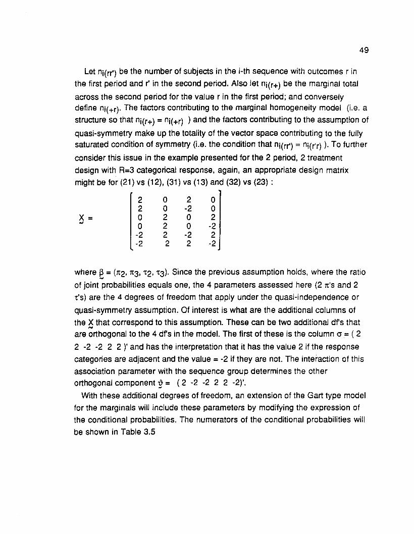
49

Let ni(rr') be the number of subjects in the i-th sequence with outcomes r in

the first period and r' in the second period. Also let ni(r+) be the marginal total

across the second period for the value r in the first period; and converselydefine ni(H)' The factors contributing to the marginal homogeneity model (Le. a

structure so that ni(r+) = ni(H) ) and the factors contributing to the assumption of

quasi-symmetry make up the totality of the vector space contributing to the fullysaturated condition of symmetry (Le. the condition that ni(rr') = ni(r'r) ). To further

consider this issue in the example presented for the 2 period, 2 treatment

design with R=3 categorical response, again, an appropriate design matrix

might be for (21) vs (12), (31) vs (13) and (32) vs (23) :

2 0 2 02 0 -2 0

X= 0 2 0 2oJ

0 2 0 -2-2 2 -2 2-2 2 2 -2

where ~ = (1t2, 1t3, t2, t3). Since the previous assumption holds, where the ratiooJ

of joint probabilities equals one, the 4 parameters assessed here (2 1t'S and 2

t'S) are the 4 degrees of freedom that apply under the quasi-independence or

quasi-symmetry assumption. Of interest is what are the additional columns of

the X that correspond to this assumption. These can be two additional df's that-are orthogonal to the 4 dfs in the model. The first of these is the column cr = ( 2

2 -2 -2 2 2)' and has the interpretation that it has the value 2 if the response

categories are adjacent and the value =-2 if they are not. The interaction of this

association parameter with the sequence group determines the other

orthogonal component ~ = (2 -2 -2 2 2 -2)'.

With these additional degrees of freedom, an extension of the Gart type model

for the marginals will include these parameters by modifying the expression of

the conditional probabilities. The numerators of the conditional probabilities will

be shown in Table 3.5

50

Table 3.5

Numerators of Conditional Probabilities with three response levels

and inclusion of association parametersi2.ll ll2lexp(1t2 + 't2 + (J + l}) exp(-1t2 - 't2 - (J - l})

exp(1t2 - 't2 + (J - l} ) exp(-1t2 + 't2 - (J + l} )

!lli Wlexp(1t3 + 't3 - (J - l} ) exp(-1t3 - 't3 + (J + l} )

exp(1t3 - 't3 - (J + l} ) exp(-1t3 + 't3 + (J - l} )

Q2l !2Jlexp(1t3 - 1t2 - 't2 + 't3 + (J + l} ) exp(1t2 -1t3 +'t2 -'t3 - 0" - l} )

exp(1t3 - 1t2 + 't2 - 't3 + (J - l} ) exp(1t2 -1t3 -'t2 +'t3 - 0" + l})

A:BB:A

A:BB:A

SequenceA:BB:A

These 0" and l} parameters would be what Kenward and Jones (1989) would

deal with if they did not consider the diagonal cells. With the full 8 joint

probabilities, Kenward and Jones apply a general log-linear model with 4 0"

association parameters and 4 l} sequence by dependency parameters. More

detail is provided for this in Chapter 8.

The fully saturated design matrix is

2 0 2 0 2 22 0 -2 0 2 -2

x= 0 2 0 2 -2 -2oJ

0 2 0 -2 -2 2-2 2 -2 2 2 2-2 2 2 -2 2 -2

where ~ = (1t2, 1t3, 't2, 't3, 0", l}). Since this structure represents a full rank model,,.

all estimation is unrestricted maximum likelihood; thus, implying maximum

likelihood estimation is equivalent to weighted least squares. The advantage of

this relationship is that the parameter vector can be expressed as a function of

the logits via the inverse of the design matrix. For the function of logits F, ~ = X-1,..... -F and X-1 is :,.. oJ

51

2 2 1 1 -1 -1-I 1 1 2 2 1 1

X =1/12 2 -2 1 -1 -1 1N

1 -1 2 -2 1 -11 1 -1 -1 1 11 -1 -1 -1 1 -1

This information aids in assessing how the estimates of the period and

treatment effects are computed when the conditional independence of pairwise

combinations does not hold and (J and ~ have been incorporated into the model

to accommodate this.

Observe the third row of X-1 and apply this to the logit functions. Thus, the,..estimate of t2 can be viewed as the following function

t2 =1 16 {logit(81) - logit(82) } + 1 1 12 {logit(83) + logit(86) - logit(84) -logit(85)}

~ I~ ~ I~= 1/6 In { AB(12) AB(21)} + 1112 In { AB(13) AB(31)

~BA(12) 1~BA(21) ~B A (13) 1~BA(31)

'13A(23) 1~BA(32) }

~AB(23) 1~AB(32)

=1 16 { 4t2 + 4~ } + 1 112 { 4t3 - 4~ + 4 t2 - 4 t3 - 4 ~ }

= (2 13) t2 + (1 13) t2

Thus, t2 is estimated by a weight of 2/3's from the odds corresponding to (12) vs

(21) for the 2 sequences and a weight of 113 assigned to the ratio of the odds

ratios corresponding to (13) vs (31) versus that for (32) vs (23). Similarly, for theestimate of t3, a weight of 2/3's is assigned to the odds ratio for the response

(13) vs (31) and a weight of 113 is assigned to the (23) vs (32) and (12) vs (21)

response odds ratio.

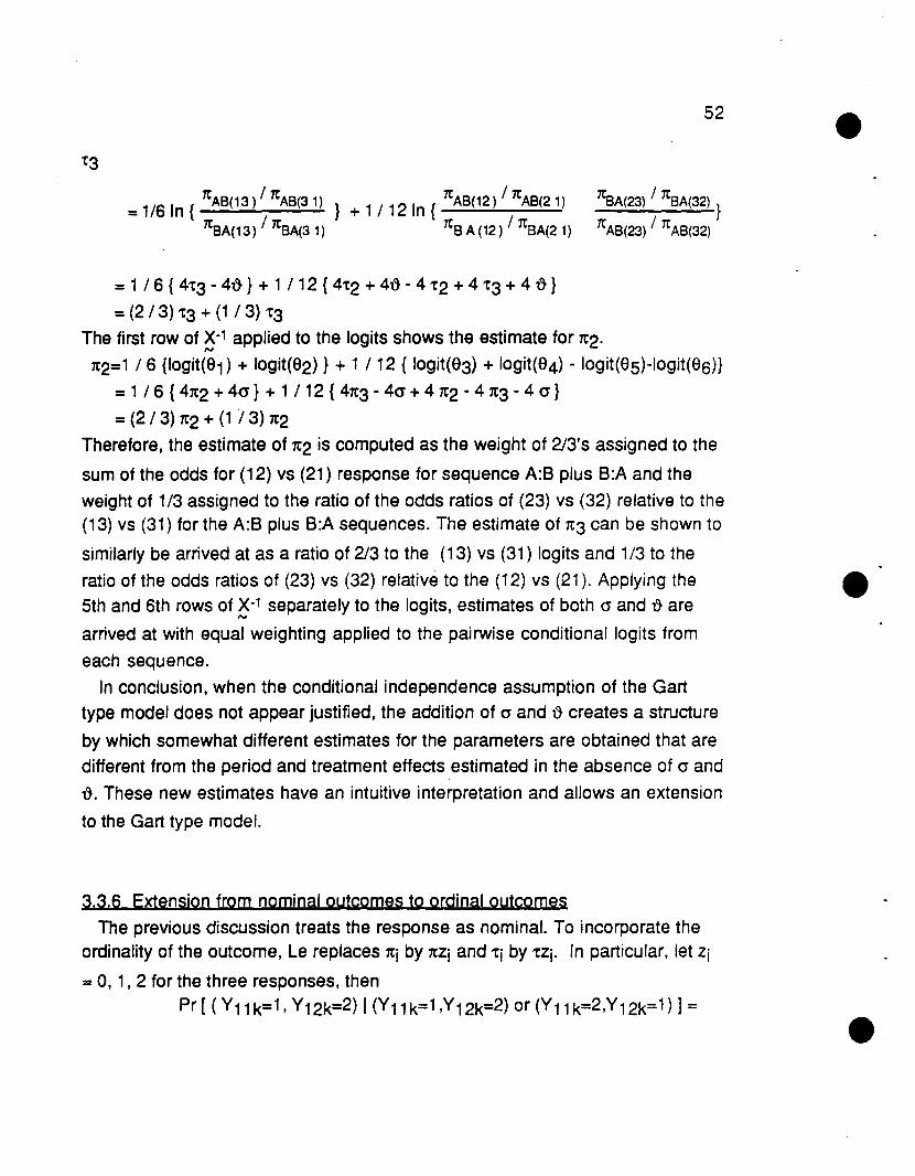
~ I~ ~ I~=1/6In{ AB(13) AB(31)} +1/12In{ AB(12) AB(21)

~BA(13) 1~BA(31) ~B A (12) 1~BA(2 1)

52

~A(23) 1~BA(32) }

~AB(23) 1~AB(32)

= 1 16 { 4t3 - 4~ } + 1112 { 4t2 + 4~ - 4 t2 + 4 t3 + 4 ~ }

= (2/3) t3 + (1 13) t3

The first row of X-1 applied to the logits shows the estimate for ~2.IV

~2=1 16 {logit(81) + logit(82) } + 1 1 12 { logit(83) + logit(84) - logit(85)-1ogit(8S)}

= 116 { 4~2 + 4cr} + 1112 { 4~3 - 4cr + 4 ~2 - 4 ~3 - 4 cr }

=(21 3) ~2 + (1 j 3) ~2

Therefore, the estimate of ~2 is computed as the weight of 2I3's assigned to the

sum of the odds for (12) vs (21) response for sequence A:8 plus 8:A and the

weight of 113 assigned to the ratio of the odds ratios of (23) vs (32) relative to the(13) vs (31) for the A:8 plus 8:A sequences. The estimate of ~3 can be shown to

similarly be arrived at as a ratio of 213 to the (13) vs (31) logits and 113 to the

ratio of the odds ratios of (23) vs (32) relative to the (12) vs (21). Applying the5th and Sth rows of X-1 separately to the logits, estimates of both cr and ~ are

'"arrived at with equal weighting applied to the pairwise conditional logits from

each sequence.

In conclusion, when the conditional independence assumption of the Gart

type model does not appear justified, the addition of cr and ~ creates a structure

by which somewhat different estimates for the parameters are obtained that are

different from the period and treatment effects estimated in the absence of cr and

~. These new estimates have an intuitive interpretation and allows an extension

to the Gart type model.

3,3,6 Extension from nominal outcomes to ordinal outcomes

The previous discussion treats the response as nominal. To incorporate theordinality of the outcome, Le replaces ~i by ~Zj and tj by tZj. In particular, let Zj

= 0, 1, 2 for the three responses, then

Pr [ ( V11 k=1, V12k=2) I (V11 k=1 ,V12k=2) or (V11 k=2,V12k=1) ] =

53

exp(1t(Z1-Z2) + t(Z1-Z2)) /

[ exp(1t(z1-z2) + t(Z1-Z2) ) + exp(1t(z2-Z1) + t(z2-Z1) ) ]

= exp(-1t-t) / [exp( -1t-t) + exp(1t + t)

Table 3.6 indicates the numerators for these conditional probabilities:

SequenceA:BB:A

A:BB:A

A:BB:A

Table 3.6

Numerators of Conditional Probabilities

where R=3 ordinal response categories!2ll !12.lexp(1t + t) exp(-1t - t)

exp(1t - t) exp(-1t + t)

!lli L1Jlexp(21t + 2t) exp(-21t - 2t)

exp(21t - 2t) exp(-21t + 2t)Q2l W.lexp(1t + t) exp(-1t - 't)

exp(1t - 't) exp(-1t + t}

The implied design matrix isX = '2 2.,J , 2 -2

4 44 -42 22 -2

where ~ = (1t, 't)'..,....

The associated odds ratios for A:B vs B:A are

OR ((12) vs (21)) = exp [-4't]

OR ( (13) vs (31) ) = exp [ -at]

OR ( (23) vs (32) ) = exp [ -4t ]

Notice the model presented is in fact the equal adjacent odds ratio model

directed at the ordinal response.

54

3,3.7 Extension to Time Dependent Coyariates

Time dependent covariates can be taken into account when there are

covariates values that change over time, Le., they have different values at each

period. These covariate values can be continuous or categorical. As an

example, before comparing treatments to improve a skin condition, the

condition is graded as to severity (mild, moderate or severe). For another study

on the recurrence of headaches, at the beginning of each period, the severity of

the headache is measured as moderate or severe. This value will change for

each period of observation.Let Xijk by the value of a baseline or period assessment that changes for each

of the j periods, for the i-th sequence group for the k-th subject. For adichotomous Xijk =0 or 1 in the classic 2 x 2 design, each period contributes

the presence or absence of some covariate condition.

The conditional joint probabilities are shown in the Table 3,7 below. The

treatment and period effects are defined from a center point coding scheme asbefore. To the marginal probability, one adds the parameters 8 Xijk to the other

factors to reflect the amount that the covaraite contributes at the Hh period.

Table 3.7

Conditional Joint Probabilities

Time Dependent Covariates

Sequence

A:BB:A

Conditional Joint Prob,

UQl LOll-1t + t + ~ x11 k 1t - t + ~ x12k

-1t - t + ~ x21 k 1t + t + ~ x22k

-21t +2t + 8(X11 k - X12k)

-21t - 2t + 8(X21 k - x22k)

From the logit it can be observed that the k-th subject difference across the

periods describes the contribution of the covariate effect. For a covariate with

values 0 and 1, there are three possible values for the difference across the

periods, -1 , 0 and 1. Grouping the subjects by strata according to this difference

value yields three strata on which to compare the sequence groups with respect

to the discordant responses. Thus, the 6 x 3 design matrix shown below allows

55

for estimation of the effects ~ = (1t,t,ro) where ro is the effect of the covariate..,through 0 (Xi1 k - Xi2J<)·

X = -2 2 0oJ -2 2-1

-2 2 1-2 -2 0-2 -2 -1-2 -2 1

When the covariate has three discrete values, there are ten rows to the

design matrix representing the 5 difference values by the two sequence groups.

This strategy also handles the continuous covariate, by noting that situation

corresponds to a standard logistic regression where one of the factors is a

continuous difference score. The value associated with the period effect is -2

and the value for the treatment effect is 2 for the sequence A:B and -2 for the

sequence B:A.

3.3.8 Extension to gartjally ordered data for survival

This chapter has dealt with binary, nominal and ordinal outcomes for the 2 x 2

design. Another type of extension is when there is a partial ordering to the

response vector. Therefore, it can at least be considered a nominal response;

however, since there is only a partial ordering structue it cannot be viewed as

purely ordinal.Survival data falls in this category. Consider the following situation: Let Yitjk

be the k-th subject's outome within the i-th sequence (i=1, 2) for the t-th time

interval within the j-th period (t=1, 2, j=1, 2). There are four possible outcomes

any subject can have for either period: F1 =failed at the first time interval (and

thus for the treatment of this period is not eligible for continuing to the second

time interval), WS1 = did not fail at the first time interval but withdrew before the

second time interval, F2=failed at the second time interval but not the first, S2=

survived both time intervals. Note for many clinical trials, this event of failure

may be that a side effect developed preventing the administration of any drug in

subsequenct intervals. The partial ordering exists as an ordering to F1 , F2 and

S2 ( Le. F1 is worse than F2 is worse than S2) and another ordering to F1 <

W51. For ease of representation, henceforth the outcomes F1, W51, F2 and 52

will be denoted as 1, 2, 3 and 4 respectively.

56

Since this outcome can at least be considered a nominal response, a model

will be developed first where the outcome has 4 nonordered levels. Restrictions

applied to the parameters will allow for the partial order structure to be taken

into account. The nominal model of Section 3.3.6 will apply. Marginal

probabilities are constructed for the outcome as before and discordant pairs of

observation are observed.

Since there are four possible responses, there are three estimable periodeffects (7t1 , 7t2 and 7t3) relative to a coding with the 7t4 effect as a reference cell

for the first period and three estimable treatment effects t1 , t2 and t3 relative to

the reference of t4 for treatment B. These are assessed across a comparison of

the following pairs: 12 vs 21, 13 vs 31, 14 vs 41 , 23 vs 32, 24 vs 42 and 34 vs

43. The following table displays the natural logarithm of the numerators of the

conditional probabilities.

Table 3.8

Conditional Joint Probabilities and Design Matrix

Four Nominal Survival LevelsCond'n Joint Prob ItU2l J.2ll Kl Kg ~ 11 12- ~

A:B 1t2 + 't1 1t1 + 't2 -1 1 0 1 -1 0

S:A 1t2 + 't2 1t1 + 't1 -1 1 0 -1 1 0Wl illl

A:S 1t3 + 't1 7t1 + 't3 -1 0 1 1 0 -1B:A 1t3 + t3 7t1 + t1 -1 0 1 -1 0 1

ll.4l !.illA:B 't1 7t1 -1 0 0 1 0 0

S:A 0 7t1 + 't1 -1 0 0 -1 0 0

12Jl Q2.lA:B 1t3 + 't2 7t2 + 't3 0 -1 1 0 1 -1

S:A 1t3 + 't3 7t2 + 't2 0 -1 1 0 -1 1

LW L42lA:B 't2 7t2 0 -1 0 0 1 0

B:A 0 7t2 + 't2 0 -1 0 0 -1 000 aal

A:S 't3 1t3 0 0 -1 0 0

S:A 0 1t3 + t3 0 0 -1 0 0 -1

57

1 0 -1 01 0 1 0

2 0 -2 0

2 0 2 0

2 -1 -2 12 -1 2 -1

3 -1 -3 1

3 -1 3 -1

1 0 -1 0

1 0 1 0

This structure can be further refined by incorporating the partial ordering

available through the survival framework. Consider that in regards to favorable

outcomes, the response 1 is worse than 3 is worse than 4. The other

relationship that exists is that response 1 is worse than response 2 in respect to

a positive outcome. In the purely ordinal case of Section 3.3.6, the equal

adjacent odds ratio assumption was made. Similarly for this partial ordering onecould assume that 1t3 =1t, 1tl = 2 1t and 't3 =t, tl = 2 'to This reduced structure

modifies table 3.8 to the following :

Table 3.9


Partial Ordering StructureS§.g Cond'n Joint Prob

L12.l!.2.ll K 1[2, I 1£

-1 1 1 -1

-1 1 -1 1

A:B 1t2 + 't 1t + 't2

B:A 1t2 + 't2 1t+'t

lli.l UllA:B 21t + 't . 1t + 2't

B:A 21t + 2't 1t+'t

llil !.illA:B 31t +'t1 1t + 3't

B:A 31t + 3't 1t+'t

!2.3l Q2lA:B 21t + 't2 1t2 + 2't

B:A 21t + 2t 1t2 + 't2

~ ~A:B 31t +'t2 1t2 + 3't

B:A 31t + 3t 1t2 + 't2

Wl !!JlA:B 31t + 2t 21t + 3t

B:A 31t + 3't 21t + 2t

Notice for each of the parameters, a 3 degree of freedom is reduced to a 2

degree of freedom test (where one degree of freedom is assigned to each of the

relationships). This reflects the partial ordering structure different from the purely

58

ordinal case where the 3 degree of freedom test is reduced to one degree of

freedom. For instance, for treatment this corresponds to a simultaneous test of t

and t2. A one degree of freedom test is feasible based on a weighted average

of t and t2. One logical choice of weighting would be to use the inverse

variance.

Another logical reduction for survival data is to compare the two periods for

failure vs success in each time interval. For time interval 1, a failure is the first

outcome (1) and a success is either of the outcomes 2,3 or 4. For the time

interval 2, a failure is response 3 and a success is response 4. This implies

comparison of the disjoint pairs 12, 13 and 14 (all combined) vs 21, 31 and 41

(all combined) at time interval 1 and 34 vs 43 at time interval 2. Extending the

principles of Gart, the concordant pairs will not be considered. Also, the pairs 23

vs 32 and 24 vs 42 are not used for this model because they compare events

from different time intervals. The following table indicates the In of the

numerators of the conditional probabilites assuming period and treatment

effects and the corresponding fully specified design matrix.

Table 3.10


Failure vs Success at each Time Interval~ Time interval (Em !.Sfl Design Matrix

K I ill L..rnA:B 1 t 1t -1 1 0 0

B:A 1 0 1t+t -1 -1 0 0

A:B 2 t 1t -1 1 1 1

B:A 2 0 1t+t -1 -1 1 -1

The factor m corresponds to a time interval effect and t * m is the interaction of

the treatment with time interval. These two components are the additional

degrees of freedom needed to saturate the design space.

The model can be viewed as a refinement to the purely nominal model withthe following rationale: allow 1t (from this model) =1t1 (from the purely nominal

model) and t =t1 for the first time intreval and 1t (again from this model) = 1t3

and t =t3 for the second time interval.

59

Aside from these models, an ad hoc procedure to compare the effectiveness

of the treatment across the sequence groups is to implement an extended

Mantel-Haenszel test. Tables are created, controlling for the grouping of time

interval in the survival vs failure approach or controlling for the disjoint pairs

compared in the purely nominal or partially ordered models. This results in an

intuitive nonparamteric test which compares on sequence group vs the various

pairs of responses at the two periods.

3.4 Other two period. two treatment designs

Gart's method for the 2 period design with sequences A:8 and 8:A can be

extended to other designs. The following sections will describe two of these

designs which incorporate additional sequence groups for the two treatments.

For each of these designs, the marginal probabilities consistent with Gart's

framework will be shown and from this, the logits, design matrices and

definitions of parameters will be introduced. Attention will be directed towards

. the estimability of parameters, particularly the carryover effect and expression of

the odds ratio. For each of these designs, the accommodation of a nominal or

ordinal response will be presented similar to the extension in section 3.3.4 and

3.3.6.

3.4.1 2 period I 2 treatment I 4 seguences

This two period design randomizes the patients to one of the following

sequences A:A, A:8, 8:A, or 8:8 indexed by i=l, 2, 3, 4. Elswick and Uthoff

(1989) present a nonparametric approach for this design with a continuous

outcome. They note that the advantage of this design is that it is optimal in the

presence of unequal carryover effects. For this design with a binary response,

the coefficient for period effect, as with the classical model, will be defined asxx=1 if period 1, x1t=-l if period 2. The x't=l be the coefficient term that

corresponds to treatment A positive and x't=-1 if treatment 8 positive and thecarryover xA=1 if treatment A carries to period 2 and xA=-1 if treatment 8 carries

to period 2. These correspond respectively to the effects 1t, 't and A. First, the

marginal probabilities for the positive event (Yijk=l) are shown in the first two

60

columns in Table 3.11. The complement probabilities are Pr(Yijk=O) = 1

Pr(Yijk=1 ).

Table 3.11

Marginal Probabilities and Conditional Numerators

Two Periods / Two Treatments / Four Sequences

Period 1 Period 2 Conditional

Numerators

A:Aexp(<\ + 1t + t)

1 + exp(<\+ 1t+ t)

exp(<\ - 1t + t + A)exp(1t+t) exp(-1t+t+A)

1 + exp(<\- 1t + t +A)

A:8exp(ak + 1t + t) exp(<\ - 1t - t + A)

exp(1t+t) exp(-rt-t+A)1 + exp(<\+ rt + t) 1 + exp(C\- rt - t +A)

e

8:Aexp(C\ + 1t - t) exp(uk - rt + t - A)

exp(1t-t) exp(-rt+t-A)1 + exp(C\+ 1t - t) 1 + exp(C\- 1t + t -A)

8:8exp(C\ + 1t - t)

1 + exp(C\+ 1t - t)

exp(C\ - 1t - t - A)exp(1t-t) exp(-1t-t-A)

1 + exp(~- 1t - t -A)

The last two columns of Table 3.11 display the numerators of the conditional

probabilities conditioned on the pair of discordant outcomes.

The logits from these conditional probabilities :

logit (81) = In ( 1t A:A (10) / 1t A:A (01) )

61

= In [ (e1t+t) / (e-1t+t+A + e1t+t)J / [e-1t+t+A) / (e-1t+t+A + e1t+t)J

= 21t-A

logit(82) = 21t + 2t - A

logit(83) = 21t - 2t + A

logit(84) = 21t + A

(3.4.1 )

T~U~ the[d;Signomat~~XJto model these discordant counts is

I\; 2 2 -12 -2 12 0 1

where ~ = (1t,t,A)'. Note that each row of the design matrix corresponds to one....of the sequences.

In contrast to the classical design, this design allows for estimation of A. Thus,

these additional sequences provide critical information when the assumption of

nonsignificant carryover cannot be asserted a priori. The odds ratios for

sequences 1 vs 2, 1 vs 3, 1 vs 4, 2 vs 3, 2 vs 4, and 3 vs 4 have the following

expressions, respectively: e -2t, e 2t-2A, e-2A, e4t-2A, e-2t-2A, e-2t.

Also, a further separation of the carryover effect is possible by defining 2carryover effects such that AA:A=1 if treatment A carries to period 2 when period

2 receives treatment A and AA:A=-1 if treatment 8 carries to period 2 when

again treatment A occurs in period 2. Thus, this carryover reflects A vs 8 with

respect to treatment A in the second period. This carryover is distinguished fromAA:S=1 if treatment A carries over to period 2 for A:B and AA:B=-1 if treatment B

carries over for B:8. The associated design matrix is

x="'" [I

010201-2 -1 0o 0 -1

where ~ = (1t, t, AA:A, AA:8)'. In order to verify that these parameters are~

correct, note that adding the columns corresponding to AA:A and AA:B yields

the column corresponding to A. Thus, they span the same vector space. Also,

notice that the subtraction of the two columns for AA:A and AA:8 yields the

62

column (1 -1 -1 1)' which is orthogonal to the three columns of the first model.Thus, separation into the 2 A'S correctly includes the final degree of freedom.

Instead of a binary response, this study design could also be appropriate for a

nominal or ordinal response. The marginal probabilities for the r-th response

level are displayed below in the first two columns of Table 3.12. When r=1 forthe first response, <Xk1 =1t1 ='t1 =A1 =0. The last two columns of Table 3.12

indicate a general expression for the numerators of the conditional probabilitiesfor the discordant pairs (r1 ,r2) and (r2.r1) where r1 ~ r2.

For each of the sequences i=1 , 2, 3, 4, the logit for the discordant pairs is logit= In (1ti(r2,r1) /1ti (r1 ,r2)). For the example of the trivariate response levels 1, 2

and 3, Table 3.13 displays the numerators for the conditional probabilities and

the associated logits.

The associated design matrix, shown below, models 6 degrees of freedom for

the R-1 period effects, R-1 treatment effects and R-1 carryover effects where

R=3. The remaining 6 degrees of freedom prOVide a test for goodness of fit

equivalent to testing for quasi-independence (df=4) and homogeneity of

carryover across second period treatments (df=2).

x= 2 0 0 0 -1 0.J

2 0 2 0 -1 02 0 -2 0 1 02 0 0 0 1 00 2 0 0 0 -10 2 0 2 0 -10 2 0 -2 0 10 2 0 0 0 1

-2 2 0 0 1 -1-2 2 -2 2 1 -1-2 2 2 -2 -1 1-2 2 0 0 -1 1

where ~ = (1t2, 1t3, 't2, 't3, A2, A3)'. From this matrix, initial hypotheses toN

consider would be A2=A3= 0, 't2='t3=0, and 1t2=1t3=0.

ugJ:l1

exp(1tr2-1tr1 +'tr2-"[r1 +A'1)

exp(1tr2-1tr1 -tr2-tfl-Af1)

exp(1tr2 -1tr1 -tr2+"[r1-Aq)

exp(Jtr2-1t'1 +'tr1 +'tr2+\1)

Ul~l

exp(1tfl

-1tr2-tr1 -tr2-\2)

exp(Jtr1 -1tr2-tr1 +"[r2-Ar2)

exp(1tr1

-1tr2

+tr1

+tr2

+Ar2

)

exp(Jtr1 -1tr2+"[r1-"[r2+Ar2)

Table 3.122 Period, 2 Treatments, 4 Sequences with Nominal Response

Numerators for Conditional Prob.Marginal Probabilities

Period 1 Period 2~ ErlYH =r) PrlYi2=r)

A:Aexp(Clkr+1tr+9 exp(Clk(1tr+'tr+\)

R R1+ 'L,exp(Clkh+1th+th) 1+ 'L,exp(Clkh-lthHh+Ah)

h=2 h=2

A:Bexp(Clkr+1tr+'tr) exp(~(1t("[r+\)

R R1+ 'L,exp(Clkh+1th+th) 1+ Iexp(Clkh-1th-th+Ah)

h=2 h=2

B:Aexp(~r+1tttr) exp(~(1tr+tr-\)

R R1+ IeXp(Clkh+1th-"[h) 1+ IeXp(Clkh-Jth+th-Ah)

h=2 h=2

B:Bexp(~r+1t(9 exp(~(1t("[rAr)

R A1+ Iexp(ukh+Jth-"[h) 1+ Iexp(ukh-Jth-"[h-Ah)

h=2 h=2

0)

w

64

Table 3.13

Conditional Numerators and Logits

Nominal Response with three Levels

~umerators for Conditional Probabilities Logits (nominalresponse)

!21l U2lA:A exp(1t2+t 2) exp(-1t2+t2+A2) 21t2 - A2

A:B exp(1t2+t 2) exp(-1t2-t2+A2) 21t2 + 2t2 - A2

B:A exp(1t2-t 2) exp(-1t2+t2-A2) 21t2 - 2t2 -+= A2

B:B exp(1t2-t 2) exp(-1t2-t 2-A2) 21t2 + A2Wl Wl

A:A exp(1t3+t 3) exp(-1t3+t3+A3) 21t3 - A3

A:B exp(1t3+t 3) exp(-1t3-t3+A3) 21t3 + 2t3 - A3

B:A exp(1t3-t 3) exp(-1t3+t3-A3) 21t3 - 2t3 + A3

B:B exp(1t3-t 3) exp(-1t3-t3-A3) 21t3 + A3ml Wl

A:A exp(1t3-1t2+t2+t3+A2) exp(1t2-1t3+t2+t3+A3) -21t2 + 21t3 + A2 -A3 eA:B exp(1t3-1t2-t2+t3+A2) exp(1t2-1t3+t2-t3+A3) -21t2 +21t3 -2t2 +2t3+

A2 -A3

B:A exp(1t3-1t2+t2-t3-A2) exp(1t2-1t3-t2+t3-A3) -21t2 +21t3 +2t2 -2t3

-A2+A3

B:B exp(1t3-1t2-t2-t3-A2) exp(1t2-1t3-t2-t3-A3) -21t2 + 21t3 - A2 +A.3

Use of the equal adjacent odds ratio model will allow one to incorporateordinality to the response. With this same trivariate response, let Zj=O, 1, 2 such

that the parameters are 1ti=1tZj, tj=tZj and Aj=Azj. Table 3.14 displays these

logits based on this substitution of 1t2=1t, 1t3=21t, t2=t, t3=2t, A2=A, A3=2A into

Table 3.13.

(12) (21)

(13) (31)

(23) (32)

A:AA:BB:AB:BA:AAB

B:AB:BAAA:BB:AB:B

21t - A21t + 2't - A21t - 2't + A21t + A41t - 211.41t + 4't - 211.41t - 4't + 211.41t + 211.21t - A21t + 2't - A.21t - 2't + A

21t + A

65

The parameter vector for the corresponding design matrix is J3=(1t,'t,A)' , thus

goodness of fit is assessed with 3 additional degrees of freedom or 9 degrees of

freedom in all.

3.4.2 2 period / 2 treatment / 3 seguences

The sequences administered in this design are A:A, P:A and P:P, where P is a

placebo treatment. This study is a subset of the one just presented in sectionI

3.4.1 where only the first, third and fourth sequences are administered.. With

this investigation, treatment A is expected to produce a positive effect such that

it is considered unethical to administer the sequence A:P once the results of

period 1 have been reviewed. A further design feature that can be incorporated

is that subjects are often assigned with randomization in varying proportions.

Typical uses of this study.may allot .5, .25, .25 of the subjects to the three

sequence groups respectively.

66

The first, third and fourth rows of Table 3.11 are applicable here as are the

first, third and fourth logits from equations 3.4.1. Thus,

~ =[2 0 -1 J2-2 1

201

where ~ = (1t, 't, A)'. Note that with this design it is not possible to separate A into....estimable AA:A and AP:A.

For the nominal outcome, the 1st, 3rd, and 4th rows of Table 3.12 are

included. Thus, looking at the corresponding logits yields the following design

matrix where the goodness of fit is assessed with 3 degrees of freedom.X = 2 0 0 0 -1 0... 2 0 -2 0 1 0

2 0 0 0 1 0o 2 0 0 0-1o 2 0 -2 0 1o 2 0 0 0 1-2· 2 0 0 1-1-2 2 2 -2 -1 1-2 2 0 0 -1 1

where ~ = (1t2, 1t3, t2, t3, 1..2, 1..3)'. The ordinal response is incorporated by,..similarly omitting the second, sixth and tenth logits displayed in Table 3.14.

3,5 Example

An example to illustrate the two period, two treatment, 4 sequence design

considers a multicenter clinical trial for investigating pain relief. Subjects were

randomized to one of the 4 sequence groups receiving either one or both of the

2 active treatments A and 8. 80th treatments A and 8 have been observed to be

effective for relief of pain relative to placebo in previous studies, so a major

issue of comparison is between treatments A and B. The observed outcomes

were 0 = none to mild relief vs 1=moderate to substantial relief. Subsets of this

data have been extracted from the actual study for pedagogical purposes.

There are 2 centers where each set of 4 sequences of Sections 3.4.1 are

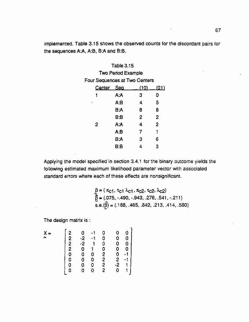
67

implemented. Table 3.15 shows the observed counts for the discordant pairs for

the sequences A:A, A:8, 8:A and 8:8.

Table 3.15

Two Period Example

Four Sequences at Two Centers

Center Seg (1 0) (01 )

1 A:A 3 0

A:8 4 5

8:A 8 8

8:8 2 2

2 A:A 4 2

A:8 7 1

8:A 3 6

8:8 4 3

Applying the model specified in section 3.4.1 for the binary outcome yields the

following estimated maximum likelihood parameter vector with associated

standard errors where each of these effects are nonsignificant.

~ =(7tc1 , tc1 Ac1' 7tc2, tc2, Ac2)<oJ

~ =(.075, -.490, -.943, .276, .541, -.211)-." ,..s.e.(~) = (.188, .465, .842, .213, .414, .580)...

The design matrix is :

x= 2 0 -1 0 0 0~ 2 -2 -1 0 0 0

2 -2 1 0 0 02 0 1 0 0 00 0 0 2 0 -10 0 0 2 2 -10 0 0 2 -2 10 0 0 2 0 1

68

The goodness of fit is acceptable with X2 = 2.77, df=2, p-value=O.25. Initial

hypotheses to consider are whether there is significant period, treatment and

carryover interactions with the center effect. This is done by testing HO:

1tc1 =1tc2, HO: 'tc1 ='tc2, and HO: A.c1 =A.c2. None of these hypotheses were

rejected at a significance level of a=.05; thus indicating the parameters 1t, 't, and

A. are equivalent for the 2 centers.

A reduced design matrix implied by these contrasts isX = 2 0 -1,.,. 2 -2 -1

2 -2· 12 0 12 0 -12 2 -12 -2 12 a 1

where the estimated parameter vector is :

'2=(1t, 't, A.)',..~= ( .175, .006, -.453 )'.... ...s.e.(~) = (.135, .281, .465 )'

The goodness ;f fit is adequate at X2=7.12, df=5, p-value=.21 ; however, none of

the parameters are significant in their own right. Thus, for this study, there is no

difference in how the 2 centers respond, nor is there any period effect, and no

treatment difference between A and 8 exists.

A simplification can be investigated with the modelX= 2 a~ 2-2

2 -22 a2 a2 22 -22 a

where ~ = (1t,'t)...~" = (.164, .230),...s.e.(~") = (.133, .163)'....

69

Since 1t is still nonsignificant, it is possible to produce a simple model with only

the treatment effect, where t"=0.193 (with a standard error of t=0.1.57). The 95

% confidence interval for this is (-0.115, 0.501). Thus, there is still no treatment

difference between treatments A and 8 as observed by noting that the null value

of zero is included in the confidence interval.

70

·CHAPTER 4

LOGISTIC MODELS FOR TWO PERIOD CROSSOVER DESIGNS

FOR COMPARISON OF THREE TREATMENTS

FOCUSING ON DISCORDANT PAIRS

4,1 Introduction

This chapter will provide further extensions to the logistic modeling framework

provided in Chapter 3 for the two period crossover design where 3 treatments

have been administered. Three different designs are presented for studies with

3, 6 and 9 sequences. Of course, other combinations of interest to thee investigator are readily obtainable as these methods generalize to a variety of 2

period change over designs with any number of treatments and sequences.

These methods also have the advantage of being applicable for binary, nominal

or ordinal responses. The most common practical application of 3 treatments

involves 2 active treatments administered vs a placebo. However, 3 active

treatments could be investigated.

4,2 2 periods / 3 treatments / 3 seQuences

The two active treatments A and B and a placebo P are administered in 3

sequence groups A:B, B:P, and P:A. For the binary outcome, the period effect is

defined as before where 7t=1 if the positive response is in period 1 and 7t=-1 if

the positive response corresponds to period 2. There are two treatment effects'fA and 'fB which have value =1 if treatments A and B, respectively, yield a

positive response and =-1 if placebo yields a positive response. If there is asignificant carryover, it could be denoted by A. where A.=1 if treatment A carries to

period 2 and A.=-1 if treatment B carries to period 2.

71

Table 4.1 displays the marginal probabilities associated with a positive

response. From these probabilities, conditioning in the discordant pairs to arrive

at the logistic probabilities can be performed asPr (Yi1 =1, Yi2=0 I (10) or (01) pair) =

Pr(Yi1=1) Pr(Yi2=0) / [Pr(Yi1=1) Pr(Yi2=0) + Pr(Yi1=0) Pr(Yi2=1)]

(4.2.1 )

The numerators of these conditional probabilities are also indicated in Table 4.1.

The corresponding logits arelogit (91) = -2x -'tA + t8 + A

logit(92) = -2x - tA -2 t8 - A

logit(93) = -2x + 2tA + t8

(4.2.2)

Since there are only 3 sequences, at most 3 parameters can be estimated. Thus,

the model associated with this would be over parametrized and one mustassume that A=O in order to estimate 1t, tA. and t8. Therefore, this design for the

binary outcome is only applicable in the case that there is no carryover due to

either treatment A or B. Thus, the design matrix appropriate for 2 periods, 3

treatments and 3 sequences is

~ =[~~ ~~ -~J-2 2 1

where ~ = (x' 'tA, t8)'·....The odds ratios can be expressed as follows: for A:8 vs B:P is exp( 3t8), for A:B

vs P:A is exp (-3tA) and for B:P vs P:A is exp -3 ( tA + t8 ).

If the response for this design is nominal with response levels r=1, 2, ... R,then one models the pairwise discordant pairs (r1 • r2) vs (r2, r1) where r1 ;l!: r2

with the logistic model. Table 4.2 shows the numerators of the conditional

probabilities conditioned on the pairs, as well as displaying the marginal

probabilities used to get these. Because the carryover effects are not estimable

for the binary outcome, they should not be considered in the nominal or ordinal

case.

e eTable 4.1

2 Period / 3 Treatment /3 Sequence Groups

e

Marginal Probabilities Numerators for Conditional Prob.

~

A:B

B:P

P:A

e

Period 1Pr(Yijk=l )

exp(ak+1t+t A)

1+exp(ak+1t+tA)

exp(ak+1t+tB)

1+exp(ak+1t+tB)

exp(ak+1t-t A-tB)

1+exp(ak+1t-t A-tB)

Period 2Pr(Yijk=l )

exp(ak-7£+tB+A)

1+exp(ak-1t+tB+A)

exp(ak-1t-t A-tB-A)

1+exp(ak-1t-t A-tB-A)

exp(uk-1t+t A)

1+exp(ak-1t+tA)

e

llill

exp(1t+tA)

exp(1t+tB)

exp(1t-tA-tB)

1Q.D

exp(-1t+tB+A)

exp(-1t-t A-tB-A)

exp(-1t+tA)

e

-.....lI\J

Table 4.22 Period, 3 Treatments, 3 Sequences with Nominal Response


~

A:B

B:P

P:A

Period 1Pr(Yil=r)

exp(CXkr+1trH Ar)

R

1+ I,exp(cxkh+1thHAh)

h=2

exp(CXkr+1trHBr)R

1+I,exp(cxkh+1thHBh)

h

exp(cxkr+1tttAttBr)R

1+I,exp(cxkh+1th-tAh-tBh)

h

Period 2Pr(Yi2=r)

exp(cxkr"1trH Br)

R

1+ I,exp(cxkh-1thHBh)

h=2

exp(~r-1tr-tAr-tBr)R

1+I,exp(cxkh-1th-tAh-tBh)

h

exp(CXkr"1trH Ar)

R1+Lexp(cxkh-1th+tAh)

h

IflJ:21

exp(1tq -1t r2H Ar1 +tBr2)

exp(1tq -1tr2-tAr2-tBr2H Bq)

exp(1tq -1tr2-tAr1 +tAr2-tBq )

ll2.Jl1

exp(1tr2-1tr1 +tAr2HBr1)

exp(1tr2-1tq -tAq -tBr1 +'tBr2)

exp(1tr2 -1tq -tAr2H Aq -tBr2)

"'JW

X=

74

e Note that when r=1, ak1 =1t1 ='tA1='tB1 =0. The logits defined as In (1tj(r2,n) / 1tj

(n, r2) ) are the information used to determine the appropriate design matrix. If

the response has 3 levels, then the 3 pairs of off-diagonal combinations for each

of the 3 sequences, Table 4.3 displays the numerators for the conditional

probabilities expressed in a general equation in Table 4.2. This table also

provides the logits for the nominal response in column 3.

Out of the nine possible degrees of freedom, six of these are used to estimatethe parameters for ~ = (1t2, 1t3, 'tA2, 'tA3, 'tB2, 'tB3)" leaving only three degrees of

freedom for goodness of fit. These additional degrees of freedom correspond toa-like association parameters. The design matrix associated with this is :

2 0 1 0 -1 02 0 1 0 2 02 0 -2 0 -1 0o 2 0 1 0 -1o 2 0 1 0 2o 2 0 -2 0 -1

-2 2 -1 1 1 -1-2 2 -1 1 -2 2-2 2 2 -2 1 -1

e Initial hypotheses might be 1t2=1t3, 'tA2='tA3, or 'tB2='tB3. Testing 2'tA2='tA3 and

2'tB2='tB3 is equivalent to testing an equal adjacent odds ratio assumption for

the treatment. Implementing this type of structure would allow for the response tobe treated as ordinal. Thus, replace 1tj by 1tZj, 'tAi by 'tAZj, and 'tBi by 'tBZj where

zi=O, 1,2. The last column of Table 4.3 displays the associated logits. The

estimated parameter vector is 13= (1t, 'tA, 'tB )' and the design matrix is :X = 2 1 -1 ...~ 212

2 -2 -14 2 -24 2 44 -4 -22 1 -12 1 22 -2 -1

Table 4.3logits for 2 P / 3 T / 3 sequence design

with nominal and ordinal response with 3 levels

~ Conditional Numerators Loaits (nominal) Loaits (ordLnal}

!211 U2l

A:B exp(1t2+'tA2) exp( -1t2+'tB2) 21t2+'tA2-t B2 21t+'tA-tB

B:P exp(1t2+'tB2) exp( -1t2-t A2-tB2) 21t2+'tA2+2tB2 21t+'tA+2tB

P:A exp(1t2-t A2-t B2) exp( -1t2+'tA2) 21tr2tA2-t B2 21t-2tA-t B

Wl UJl

A:B exp(1t3+'tA3 ) exp(-1t3+'tB3) 21t3+'tA3-tB3 41t+2tA-2tB

B:P exp(1t3+'tB3) exp( -1t3-t A3-tB3) 21t3+'tA3+2tB3 41t+2tA+4tB

P:A exp(1t3-tA3-tB3) exp(-1t3+'tA3) 21t]"2tA3 -tB3 41t-4tA-2tB

(32) (23)

A:B exp(1t3-1t2+'tA3+'tB2) exp(1t2-1t3+'tA2+'tS3) -21t2+21t3-tA2+'tA3+'tB2-tS3 21t+'tA-tB

B:P exp(1t3-1t2-t A2-t B2+'tS3) exp(1t2-1t3-tA3+'tS2-tS3) -21t2+21t3-tA2+'tA3-2tS2+2tS3 21t+'tA+2tB

P:A exp(1t3-1t2+'tA2-t A3-t S3) exp(1t2-1t3-tA2+'tA3-tS2) -21t2+21t3+2tA2-2tA3+'tB2-tS3 21t-2t A-t B'-J01

76

e 4.3 2 periods / 3 treatments / 6 seQuences

This design also incorporates 2 active treatments and a placebo treatment.

However, three additional sequences are added such that the sequences are

A:B, B:A, B:P, P:B, A:P, and P:A. Koch, et al (1989) discuss this type of design for

the continuous outcome where there is a m:m:1 :1 :1:1 ratio of allocation of

subjects to the respective sequence groups. Thus, an emphasis can be placed

on comparing sequences A:B and B:A to provide a more powerful test of

treatments A vs B.

The description of the models up to this point have employed a center point

coding scheme. For this design structure, a reference cell coding scheme will be

used to show the ease with which that type of coding can be applied and

interpreted. Both types of coding provide equivalent tests but differ in the

interpretation of parameters. The parameters will have the following definitions

with reference cell coding:7[=1 if period 2, =0 otherwise

'tA=1 if treatment A has positive response, =0 otherwise

'tB=1 if treatment S has positive response, =0 otherwise

AA=1 if treatment A carries over from period 1,

=0 otherwiseAS=1 if treatment S carries over from period 1,

=0 otherwise

(4.3.1 )

For the binary outcome, Table 4.4 displays the marginal probabilities for a

positive response for each sequence groups at each period. Also included in

this table are the numerators for the conditional probabilities calculated

according to the equation presented in Chapter 3.

The associated design matrix for modeling the respective logits,

In(1ti(O1)/1ti(10)) :

x= 1 -1 1 1 0/OJ 1 1 -1 0 1

1 0 -1 0 11 0 1 0 01 -1 0 1 01 1 0 0 0

77

Table 4.42 period I 3 treatment I 6 sequence design for binary response

Marginal Probabilities Numerators forConditional Probs.

Period 1 .Period 2 (10) (01)~ Pr(Yi1 =1) Pr(Yi2=1 )

A:Bexp(cxk+'tA) exp(cxk+1t+'tB+A.A)

1+exp(cxk+'tA) l+exp(cxk+1t+t B+A.A)exp(tA) exp(1t+'tB+A.A)

B:Aexp(cxk+'tB) exp(~+1t+t A+A.B)

exp(tB) exp(1t+'tA+A.B)1+exp(cxk+'tB) 1+exp(cxk+1t+tB+A.A)

B:Pexp(cxk+'tB) exp(cxk+1t+A.B)

exp('tB) exp(1t+A.B)1+exp(cxk+'tB) 1+exp(cxk+1t+A.B)

P:Bexp(cxk) exp( cxk+1t+'tB)

1+exp(cxk) 1+exp( cxk+7t+'tB)exp(o) exp(1tHs)

A:Pexp(cxk+'tA) exp(cxk+1t+A.A)

exp('tA) exp(7t+A.A)1+exp(cxk+'tA) 1+exp(cxk+7t+A.A)

P:Aexp(cxk) -exp(cxk+1t+tA)

exp(o)1+exp(cxk) 1+exp(cxk+1t+tA)

exp(7t+'tA)

78

e where ~ = (x. tA, tB. AA. AB)'· An initial hypothesis to investigate is whether

AA=AB=A. The inclusion of just one carryover effect implies a further reduction.

Note that the additional sequences 3 through 6 provide amply information to

estimate carryover effects as well as treatment and period effects.

For the nominal outcome, the response at each period can take the values r=1,

2•... A. Hence. one has (~) disjoint pairwise combinations to condition- on; and

from these probabilities a logistic model is applied to assess period, treatment

and carryover effects.

Table 4.5 displays the marginal probabilities for the r-th response. Also.

provided in this table is a general expression for the numerator of the conditionalprobability of the response pair (r1. r2). Note when r=1,

ak1=x1 =tA1=tB1 =AA1=AB1 =0 to provide identifiability of parameters.

If we assume that the outcome has 3 response level (R=3), then one canestimate 2x's. 2tA'S, 2tB'S, 2AA'S and 2AB's. The following Table 4.6 indicates

what the logits would be with which one could determine the rows of an

appropriate design matrix.

The logits for the ordinal response are also shown in Table 4.6 where thee following substitutions are made: 1t2=1t, x3=21t, tA2=tA. 'tA3=2'tA' tB2='tB,

'tB3=2'tB. AA2=AA, AA3=2AA, AB2=AB, and AB3=2AB. These equivalences are

consistent with the assumption of the equal adjacent odds ratio model. Thefollowing design matrix is_ applicable for ~ = (x, 'tA, tB, AA, AB) :

AI

I

x = -1 -1 -1 -1 -1 -1 -2 -2 -2 -2 -2 -2 -1 -1 -1 -1 -1 -1...,1 -1 0 0 1 -1 2 -2 0 0 2 -2 1 -1 0 0 1-1

-1 1 1 -1 0 0 -2 2 2 -2 0 0 -1 1 1 -1 0 0

1 0 0 0 -1 0 -2 0 0 0 -2 0 -1 0 0 0 -1 0

0-1 -1 0 0 0 0 -2 -2 0 0 0 0 -1 -1 0 0 0

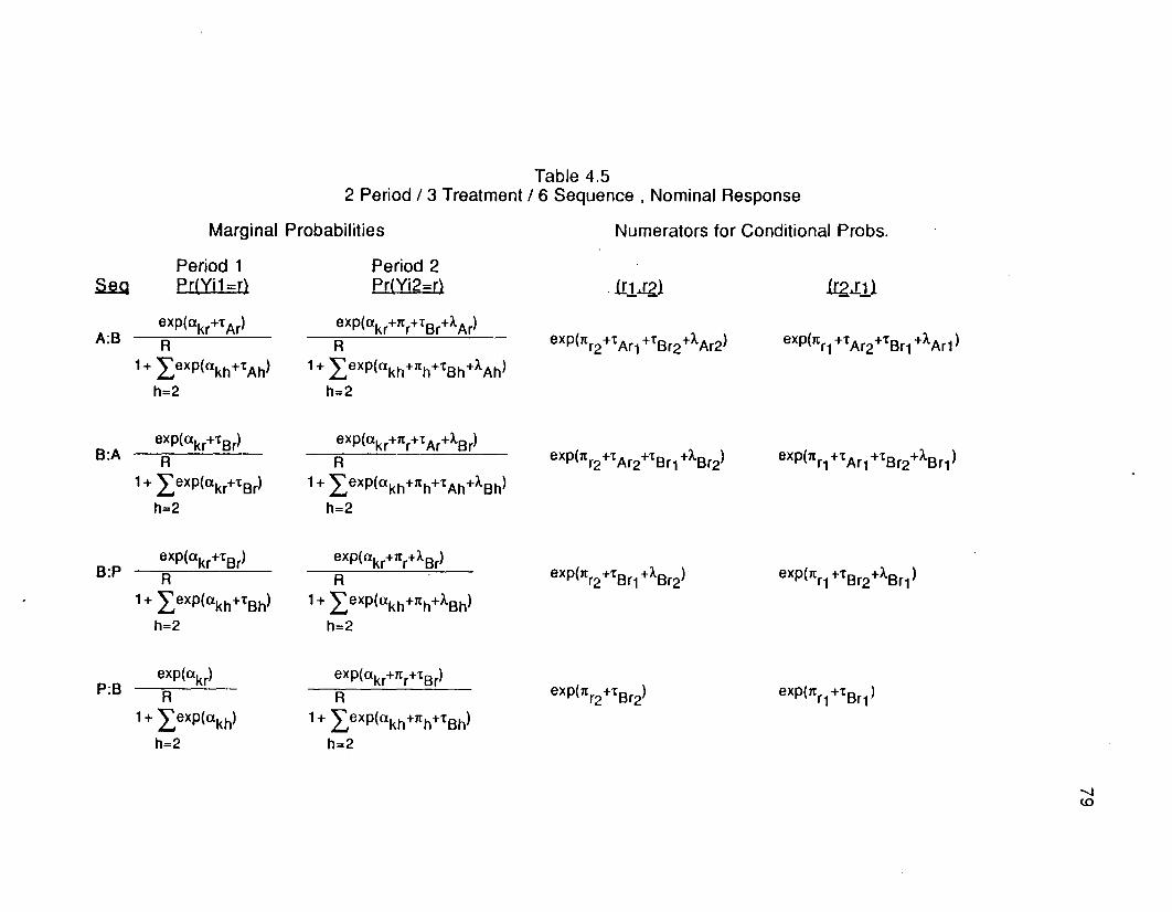
llg.Il1

exp(1tq H Ar2+'tSq +AAr1)

exp(1tr1

+'tSr2+ABr1

)

exp(1tq +'tSq )

exp(1tq +tAq +'tBr2+ABq )

1r1J:21

exp(1tr2

+'tSr2

)

exp(1tr2

+tSr1

+ASr2

)

exp(1tr2H Arl H Sr2+AAr2)

exp(1tr2+tAr2+tSq +Asr2)

Table 4.52 Period / 3 Treatment / 6 Sequence. Nominal Response

Numerators for Conditional Probs.Marginal Probabilities

Period 1 Period 2~ ~r{Yl1;:r) Pr{Yi2~r)

A:Bexp(Clkr+tAr) exp(Clkr+1trH Sr+AAr)

R R

1+ I,exp(ClkhHAh) 1+ I,exp(Clkh+1th+tSh+AAh)

h=2 h=2

B:Aexp(Clkr+'tBr) exp(Clkr+1trH Ar+ABr)

R R

1+ I,exp(Clkr+'tSr) 1+ I,exp(Clkh+1thHAh+ASh)

h=2 h=2

B:Pexp(Clkr+tSr) exp(Clkr+1tr+ASr)

R --R

1+ I,exp(Clkh+'tSh) 1+ I,exp(Clkh+1th+ASh)

h=2 h=2

P:Bexp(Clkr) exp(Clkr+1trHSr)

R R1+ I exp(Clkh) 1+ Iexp(Clkh+1th+'tSh)

h=2 h=2

-....,J(,0

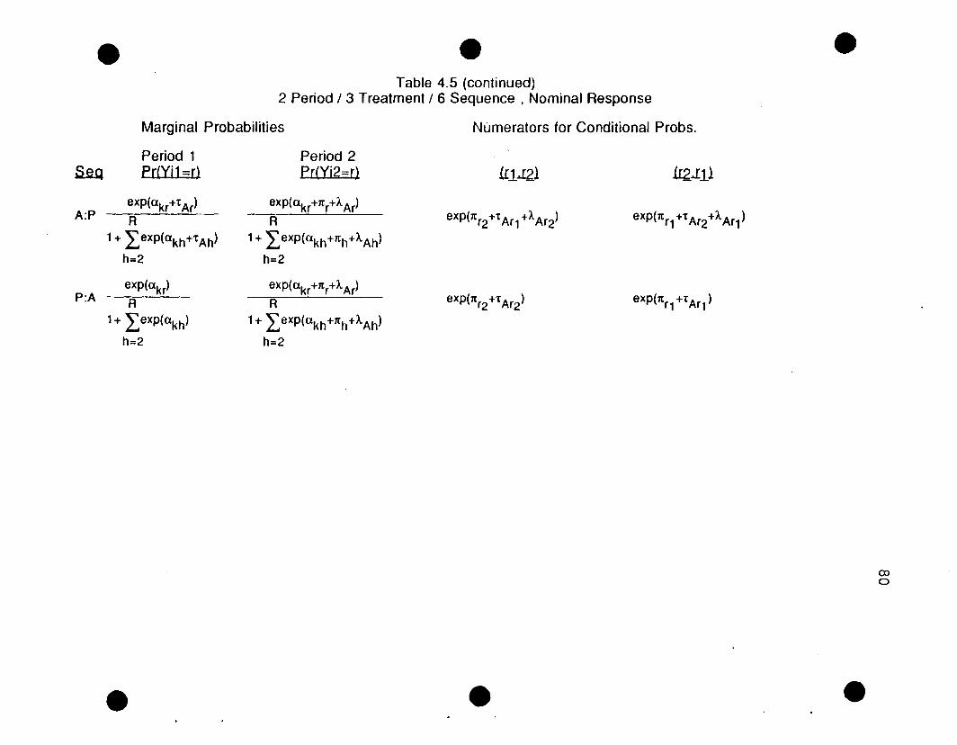
e eTable 4.5 (continued)

2 Period / 3 Treatment / 6 Sequence. Nominal Response

e

Numerators for Conditional Probs.

£e.g

Marginal Probabilities

Period 1Pr(Yi1 =r)

Period 2Pr(Yi2-r) 111,.I21 ll2..Il1

A:P

P:A

exp(akrHAr)

A

1+ Iexp(akh+'tAh)

h=2

exp(akr)

A1+ Iexp(akh)

h=2

e

exp(akr+1tr+1..Ar)

A

1+ I exp(akh+1th+AAh)

h=2

exp(akr+1tr+1..Ar)

A1+ Lexp(akh+1th+AAh)

h=2

exp(1tr2H Ar1 +AAr2)

exp(1tr2+tAr2)

e

exp(1tr1 H Ar2+1..Ar1)

exp(1tq +tAq)

e

eno

Table 4.6Logits for 2 P / 3 T / 6 sequence design

with nominal and ordinal response with 3 levels

~ Conditional Numerators Loaits (nominal) Loaits (ordinal)

L2..ll U2l

A:8 exp(tA2) exp(1t2+'tB2+AA2) -1t2+'tA2-t B2-AA2 -1t+tA -tB-AA

8:A exp(tB2) exp(1t2+'tA2+AB2) -1t2- t A2+'tB2-AB2 -1t-tA+tB-AB

8:P exp(tB2) exp(1t2+AB2) -1t2+'tB2-AB2 -1t-t B-AB

P:8 exp(O) exp(1t2+'tB2) -1t2-t B2 -1t-t B

A:P exp(tA2) exp(1t2+AA2) -1t2+'tA2-AA2 -1t-tA-AA

P:A exp(O) exp(1t2+'tA2) -1t 2-'tA2 -1t-tA

Qll LUlA:8 exp(tA3) exp(1t3+'tB3+AA3) -1t3+'tA3-t B3-AA3 -21t+2'tA-2'tB-2AA

8:A exp('tB3) exp(1t3+'tA3+AB3) -1t3-'tA3+'tB3-AB3 -21t-2tA+2tB-2AB

8:P exp(tB3) exp(1t3+AB3) -1t3+'tB3-AB3 -21t-2tB -2AB

P:8 exp(O) exp(1t3+'tB3) -1t3

-'tB3 -21t-2'tB

ex>......

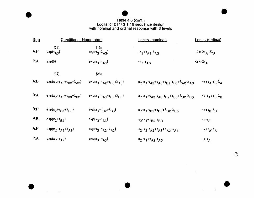
e eTable 4.6 (cont.)

logits for 2 P / 3 T / 6 sequence designwith nominal and ordinal response with 3 levels

e

~ Conditional Numerators Loaits (nominal) Loaits (ordinal)

Wl LUlA:P exp(tA3) exp(Jt3+AA3) -Jt3+tA3-AA3 -2Jt-2tA-2AA

P:A exp(O) exp(Jt3+tA3 ) -Jt r t A3 -2Jt-2tA

LJ2l !23l

A:B exp(lt2+tA3+tS2+AA2) exp(lt3+tA2+t S3+AA3) lt2-JtrtA2+tA3+t S2-t S3+AA2-AA3 -It+tA-ts-AA

B:A exp(lt2+t A2+t S3+AS2) exp(lt3+tA3+tS2+AS3) ltrlt3+tA2-t A3-tS2+tS3+AS2-AS3 -It-tA+tS-AS

B:P exp(lt2+tS3+As2) exp(lt3+tS2+As3) ltrlt3 -tS2+tS3+AS2-AS3 -It+tS-AS

P:B exp(lt2+tS2 ) exp(7t3+tS3) 7t2 -lt3+tS2-tS 3 -It-ts

A:P exp(lt2+tA3+AA2) exp(Jt3+tA2+AA3) lt2-7trtA2+tA3+AA2-AA3 -7t+tA-AA

P:A exp(lt2+tA2 ) exp(7t3+tA3 ) 7t2 -lt3+t A2-t A3 -Jt-tA

cof\)

e e e

83

4,4 2 periods I 3 treatments I 9 seQuences

This proposed plan adds to the six sequences proposed in section 4.3 to allow

for 3 additional groupings A:A, 8:8, and P:P. For the binary outcome, Table 4.4

can be augmented with three additional rows corresponding to these new

sequences. Table 4.7 displays the marginal probabilities and the numerators of

the conditional probabilities. These additional sequences augment the following

design matrix with the last 3 additional rows.X = 1 -1 1 1 0..oJ 1 1 -1 0 1

1 0 -1 0 1101001 -1 0 1 01 1 0 0 0100101 000 11 000 0

where ~ = (1t, tA, ts, AA' AS)',.-These additional sequence groups allow for a more complicated carryoverstructure to be employed. Instead of the usual type of carryover where AA and AS

are included, one could further separate out AA such that the carryover present

in A:A is different from A:S is different from A:P. Likewise AS can be expressed as

3 components. The following design matrix displays the structure where the

carryover effects are dissected in such a manner.X = 1 -1 1 0 1 0 0 0 0N 1 1 -1 0 0 0 1 0 0

1 0 -1 0 0 0 0 0 11010000001 -1 0 0 0 1 0 0 01100000001 001 000 0 01 000 0 001 01 0 000 0 0 0 0

for ~ = (1t, tA, t8, AA:A, AA:S, AA:P, A8:A ' A8:8, A8:P )'....Similarly for the nominal outcome, Table 4.5 is augmented in Table 4.8 with 3

additional rows, where the same conditions hold when r=1.

Table 4.82 Period, 3 Treatments, 3 additional Sequences with Nominal Response


£e.g

A:A

Period 1Pr(Yi1-r)

exp(<XkrHAr)

R1+ Iexp(<XkhHAh)

h=2

Period 2Pr(Yi2-r)

exp(<Xkr+JtrHAr+AAr)

R1+ Iexp(<Xkh+Jth+'tAh+AAh)

h=2

U1..£21

exp(1tr2H Aq H Ar2+AAr2)

U2.Jl1

exp(Jtr1 H Aq H Ar2+AAr1)

exp(<Xkr+fBr) exp(<Xkr+JtrHBr+ABr)exp(1tr2H Br1 HBr2+ABr2) exp(Jt

r1H Bq H

Br2+A

Br1)B:B R R

1+ Iexp(<XkhHBh) 1+ Iexp(<Xkh+Jth+'tBh+ABh)

h=2 h=2

exp(<xkr) exp(<Xkr+Jtr)exp(1t

r2) exp(Jt

r1)P:P R R

1+I exp(<Xkh) 1+I exp( <Xkh-Jth)

h h

0001

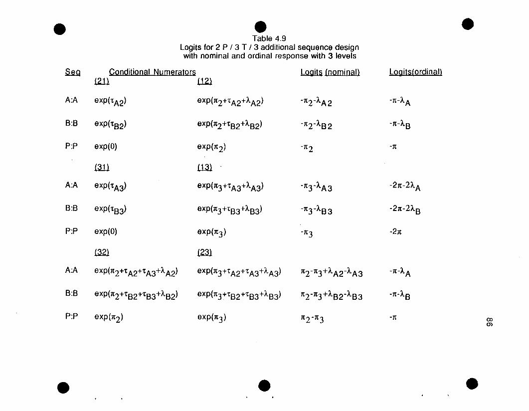
e e eTable 4.9

Logits for 2 P / 3 T / 3 additional sequence designwith nominal and ordinal response with 3 levels

futil Conditional Numerators Logits (nominal) Logits(ordinal)!2ll U2.l

A:A exp(tA2) exp(x2+t A2+AA2) -x2-AA2 -x-AA

B:B exp(tB2) exp(x2+t B2+AB2) -x2-AB2 -x-AB

P:P exp(O) exp(x2) -x2 -x

Q.ll LU1

A:A exp(tA3) exp(x3+t A3+AA3) -x3 -AA3 -2x-2AA

S:B exp(tS3) exp(x3+tB3+AS3) -x3-AB3 -2x-2AB

P:P exp(O) exp(x3) -x3 -2x

Lm .(W

A:A exp(x2+t A2+t A3+AA2) exp(x3+t A2+t A3+AA3) x2-x3+AA2-AA3 -x-AA

B:B exp(x2+t B2+t B3+AB2) exp(x3+t S2+t B3+AS3) xrX3+AB2-AB3 -x-AB

P:P exp(x2) exp(x3) x2 -x3 -x ex>m

e e e

87

Again, corresponding to Table 4.6, Table 4.9 displays the 3 additional rows

added to each of the disjoint pairs when there is a trivariate response.

Note that in both of the expressions for both the nominal and ordinal logits there

are no treatment effects since these last three sequences each involve the same

treatments for both periods.

26x5

1 -1 1 1 01 f -1 0 11 0 -1 0 1101001 -1 0 1 01 1 0 0 0

4.5 Example

An example to illustrate the design of section 4.3 considers a multicenter

clinical trial for investigating pain relief. Subjects were given 2 of 3 possible

treatments: A, B, or P=placebo. Both treatments A and B have been observed to

be effective for relief of pain relative to placebo in previous studies, so a major

issue of comparison is between treatments A and B. The observed outcomes

were 0 = none to mild relief vs 1=moderate to severe relief. This data is similar to

example in Chapter 3 and has been modified for this example. There are 2

studies each receiving the 6 sequences: A:B, B:A, B:P, P:B, A:P, P:A. Table 4.10

displays the counts for the discordant pairs. As consistent with section 4.4, the

design matrix which allows for each of the parameters to vary for the two studies

is:X,=

1 -1 1 1 01 1 -1 0 1

06x5 1 0 -1 0 1,..101001 -1 0 1 0

1 1 0 0 0

where for the i-th study ~i = (1t, 'tA, 'tB, AA, AB)'. This design matrix models tendegrees of freedom, 5 parameters for each study. However, due to the three

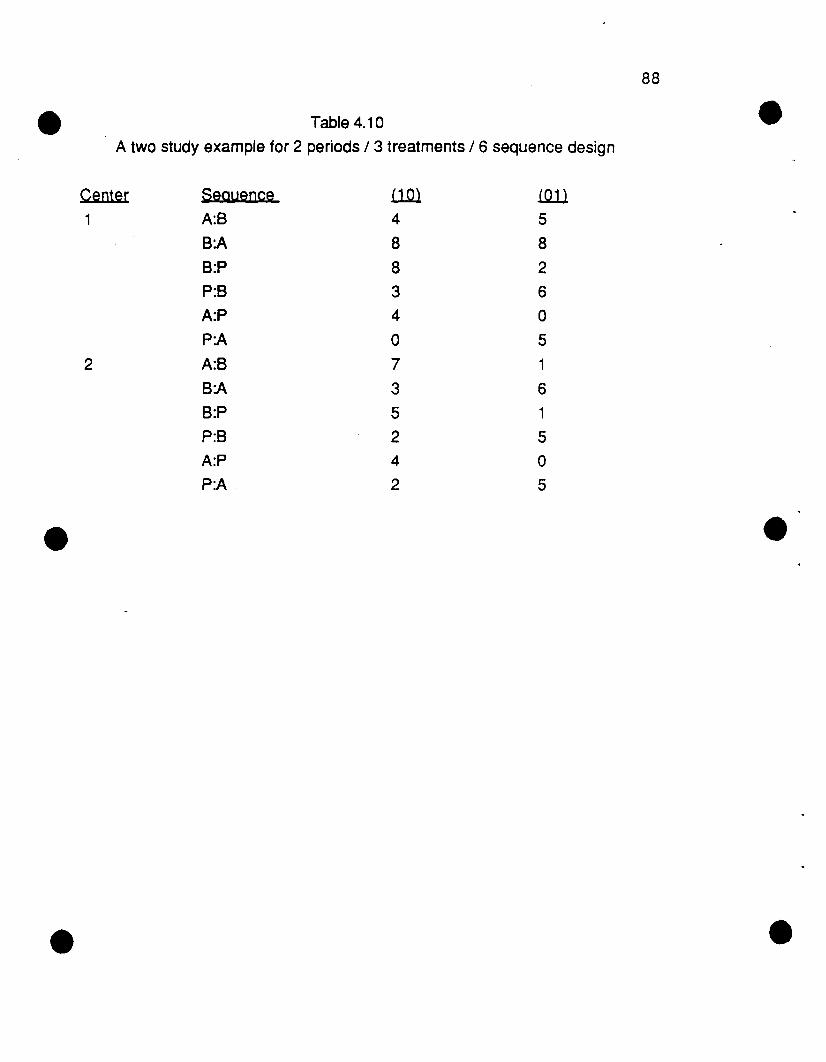
Table 4.10

A two study example for 2 periods / 3 treatments / 6 sequence design

Center

1

2

88

89

zero counts in the data table, it is only possible to estimate at most nine

parameters. Thus, the following design matrix is proposed. It models fourparameters for each study ~i= (x, 'tA, tB, A) under the assumption that AA=AB at,.,each study. Goodness of fit of this model provides a test of this assumption Thegoodness of fit is not supported with QL=18.10, df=4, p-value=0.001, thus AA=AB

is not supported.

In order to be able to estimate the parameters relative to this consideration,one strategy is to allow AA and AB to be common to the two studies, but to still

allow the period and treatment effects to differ across the studies. This modelprovides a good fit with QL = 6.01, df=4, p-value=0.20. Table 4.11 summarizes

these results. The significance of estimates from Table 4.11 reveals that the AA

parameter is not significant.

Thus, a reduced model as summarized in Table 4.12 can be considered. Thismodel also provides an acceptable fit where QL=8.33, df=5, p-value=0.14.

Finally, one can conclude a significant carryover exists for treatment B's effect

from period 1. Furthermore treatment B is significantly superior to both treatment

A and the placebo for the second study (while treatment A is not noted as

different from placebo). However, for the first study there are both significant

treatment A and B effects. There is also a significant period effect for both of the

studies. Of further interest is that the 3 degree of freedom test for equality of the

three effects (x, tA, tB) across the two studies is not significant (Qw=4.40, df=3,

p-value=0.22). Thus, another reduced model could be considered where there is

no study component.

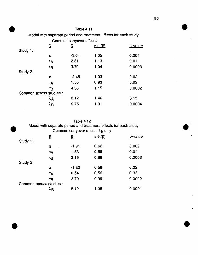
Table 4.11

Model with separate period and treatment effects for each study

Common carryover effectsa a 5.e.(6) p-value

Study 1:1t -3.04 1.05 0.004

tA 2.81 1.13 0.01

tB 3.79 1.04 0.0003Study 2:

1t -2.48 1.03 0.02

tA 1.55 0.93 0.09

tB 4.36 1.15 0.0002Common across studies :

AA 2.12 1.46 0.15

AB 6.75 1.91 0.0004

90

Table 4.12Model with separate period and treatment effects for each study eCommon carryover effect - AS only

a a s.e.(6) p-valueStudy 1:

1t -1.91 0.62 0.002

tA 1.53 0.58 0.01

tB 3.15 0.88 0.0003Study 2:

1t -1.30 0.58 0.02

tA 0.54 0.56 0.33

ts 3.70 0.99 0.0002Common across studies:

AS 5.12 1.35 0.0001

91

4,6 Piscussion

For Chapters 3 and 4, the methods of Gart were extended to 5 different

crossover designs with 2 and 3 treatments and up to 9 sequences. The logistic

model applied to the conditional probabilities for the discordant pairs can be

applied to either a binary or ordinal response.

Since a variety of 2 period crossover designs are available to the investigator,

the models presented aid in the choice of the designs. The presence of

carryover and the possibility of unequal carryover for various sequences

influence which of these designs may be more advantageous.

Thus, which parameters one wishes to estimate and how many treatments are

to be compared are issues that contribute to the selection of design. The

methods presented here have the advantages of allowing the investigator to

compare a number of treatments in a straightforward manner, with obvious

interpretation to the parameters and easy implementation with existing computer

software. Furthermore, this method allows for incorporation of covariates, such

as centers in the clinical trial or pre-study factors.

92

CHAPTER 5

LOGISTIC MODELS FOR THREE PERIOD CROSSOVER DESIGNS

FOCUSING ON DISCORDANT TRIPLES

5.1 Introduction

The focus of Chapter 5 is the three period crossover design where the

methods of Gart are extended as they were in Chapters 3 and 4 to

accommodate an additional third period. The discordant triplet of observations

will be the focus of this strategy and the information from the concordant

observations (Le., where the subjects responded with the same response on all

three periods) will not be included. The most common three period design is

where subjects are randomized to three sequence groups according to a 3 x 3

Latin square. For example, the first group receives treatments A, then 8, then C

with appropriate washout periods in between the administration of the

treatments. This group will be denoted as A:8:C. The other two sequence

groups are 8:C:A and C:A:8. A common protocol with this design is to compare

two active treatments denoted as treatments A and 8 relative to a placebo

treatment P.

In Section 5.2, the typical type of Gart framework will be considered. As in

Chapters 3 and 4, an assessment of period, treatment and carryover effects for

the binary response will be of concern. Extensions will be incorporated to allow

for modeling of the association parameters between the periods in Section 5.3.

Furthermore, one will be able to consider how this association varies for the

sequence groups. Association parameters like those of Jones and Kenward

will be briefly considered, as well as an alternate interpretation. The

equivalences that exist between these approaches allow for a comprehensive

model to gauge the dependency structure that may exist across period

measurements. In Section 5.4, it will then be shown that it is possible to extend

93

this strategy to nominal or ordinal outcomes, particularly for the three and four

category response. It is also possible to examine this method in the case of 5

response categories; however, beyond this it becomes notationally awkward to

present explicitly and so only a general outline of how to proceed is given.

Application of this strategy to a situation with six sequences from two Latin

squares will be developed in Section 5.5.

An example will appear in Section 5.6 followed by a discussion of the

strengths and limitations of applying these methods to three period crossover

studies.

5,2 Gart type logjstjc model for binary response

The analysis in this section will be restricted to those subjects randomly

assigned to one of the following three groups: A:B:C, B:C:A, C:A:B. These three

sequences represent one Latin square and will be sufficient to estimate all

parameters of interest.

Designs involving two Latin squares (Le. consisting of six sequences A:B:C,

B:C:A, C:A:B, A:C:B, C:B:A, and B:A:C) will be looked at in Section 5.5. The

advantage of 6 sequences relative to designs with just 3 sequences in one

Latin square will be that two Latin squares provide more efficient estimates

particularly with respect to carryover effects and treatment effects in the

presence of carryover effects. Furthermore, goodness of fit testing is possible

with respect to the square by effect interactions.

The outcomes of interest will be the binary response at each of the threeperiods, where the triplet response for the k-th person is denoted by (Yi1 k, Yi2k,

Yi3J<.) for the i-th sequence. The response Yijk =1 for a positive response at

period j and =0 otherwise. Thus, i indexes the sequence and j indexes the

period. The marginal probabilities at each period are expressed below in Table

5.1. Each is consistent with a logistic model assumption. The effects represent a

reference cell coding parameterization. A center point coding scheme, as well

as others, could also be employed. Chapters 3 and 4 display both types of

coding. The parameters have the following interpretation:cxk = the within subject reference probability for the k-th

subject, first period and treatment C

B:C:A

SeQuenceA:B:C

e C:A:B

94

1tj = the j-th period effect

th = h-th treatment effect for h=A, B or C

Ah = carryover effect for the h-th treatment

The ak reflect intersubject variability. They can be fixed or random effects since

they will be conditioned out in the following derivation. The resulting methods

provide an intrasubject analysis. Furthermore, in order to eliminate

redundancies for estimation purposes, it is necessary to assume that1t1 =tC=A.c=O and this convention will be reflected in Table 5.1.

Table 5.1Subject-Specific Marginal Probabilities = Pr (Yijk=1)

period Probability1 exp(ak + 'tA) / (1 + exp(<Xk + tA)

2 exp(ak + 1t2 + 'tB + AA) / 1 + exp(ak + 1t2 + tB + AA)

3 exp(ak + 1t3 + AB) / 1 + exp( ak + 1t3 + AB)

1 exp(ak + tB) / (1 + exp(ak + tB)

2 exp(ak + 1t2 + AB) / 1 + exp( ak + 1t2 + AB)

3 exp(ak + 1t3 + t A) / 1 + exp( ak + 1t3 + t A )

1 exp(ak) / (1 + exp(ak )

2 exp(ak + 1t2 + tA) / 1 + exp( ak + 1t2 + tA)

3 exp(ak + 1t3 + tB + AA) / 1 + exp( ak +1t3 +tB + AA)

To reproduce the Gart type implementation, one considers the 6 discordant

triples without using the two concordant triples (000) and (111). Conditioning

on just these six outcomes, Table 5.2 displays the numerators of the conditional

probabilities. For each sequence group there are two sets to be conditioned on.

It is necessary to separate the six joint outcomes into two groups of size three,

because the joint events (100), (010) and (001) all involve the expression exp(ak) which cancels out. The joint events (110), (101) and (011) all involve

exp(2ak) reflecting the contribution attributed to two rather than one positive

outcome across the three periods. For instance, for the first sequence A:B:C,

95

the conditional probability of the event (100) given that one of the three events

(100), (010) or (001) has occurred is shown as follows.

Let the expression

91 (a,7t,t,A)

=(1 + exp(aJ< + tA)) (1 + exp(aJ< + 1t2 + tB + AA)) (1 + exp(ak + 7t3 + AB) )

Then{ exp(aJ< + tAl / 91 (a,1t,t)..)} /

{ [exp(aJ< + tAl + exp( aJ< + 1t2 + tB + AA) + exp( ak + 7t3 + AB)] /

91 (a,x,t)..) }

= exp('tA) / [exp( 'tAl + exp( 7t2 + 'tB + AA) + exp( 1t3 + AB)]

(5.2.1 )

Similar types of quantities are obtainable for either (010) or (001) conditioned

on this set. Furthermore, again for sequence group A:B:C, the conditional

probability for (110) conditioned on the other set of events (110) I (101) and

(011) is arrived at as follows:

Pr [ (110) I (110), (101) or (011)] =

{ exp(2ak + 7t2 + 'tA + tB + AA) / 91 (a,1t,'t,A)} /

{ [exp(2aJ< + 7t2+ tA + 'tB + AA) + exp(2aJ< + 7t3 + 'tA + AB) +

exp(2aJ< + 7t2 + 7t3 + tB + AA + AB)] /

g1 (a,7t,t,A) }.

= exp(7t2+ tA + tB + AA) /

[exp(1t2+ 'tA + 'tB + AA) + exp(1t3 + 'tA + AB) + exp(1t2 + 7t3 + tB + AA+ AB)]

(5.2.2)

Maximum likelihood methods will be used to model the multiple logits where the

(001) outcome has been chosen as the reference cell for the first conditioned

set and (011) will be the other reference cell. Hence, four logits for each of the

three sequences will comprise the functions for analysis.

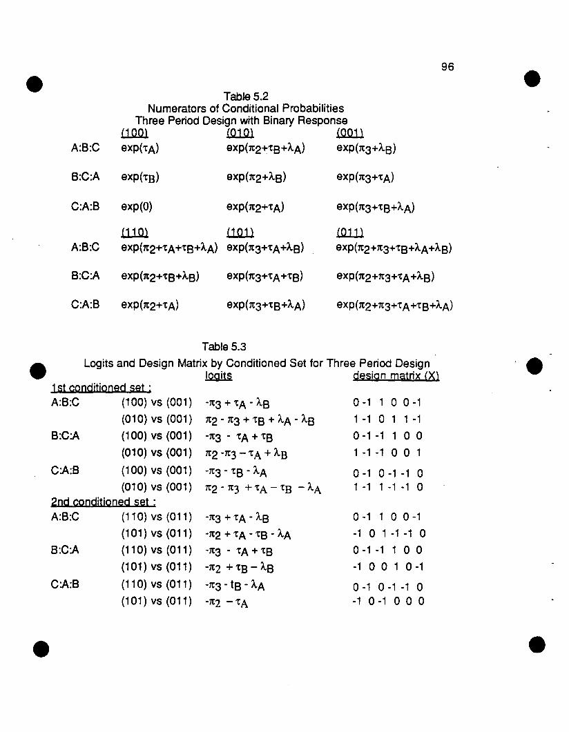
96

Table 5.2Numerators of Conditional Probabilities

Three Period Design with Binary ResponsellilOl !Q..lQl !QQ1l

A:B:C exp('tA) exp(1t2+'tB+AA) exp(1t3+AB)

B:C:A exp(tB)

C:A:B exp(O)

exp(1t3+'tA)

.LWll WillA:B:C exp(1t2+'tA+'tB+AA) exp(1t3+'tA+AB)

LO..11lexp(1t2+1t3+'tB+AA+AB)

B:C:A exp(1t2+'tB+AB)

C:A:B exp(1t2+'tA)

Table 5.3

e Logits and Design Matrix by Conditioned Set for Three Period Design e~ design matrix (Xl

1st conditioned set:A:B:C (100) vs (001) -1t3 + 'tA - AB 0-1 1 0 0-1

(010) vs (001) 1t2 - 1t3 + 'tB + AA - AB 1 -1 0 1 1 -1

B:C:A (100) vs (001) -1t3 - 'tA + 'tB 0-1 -1 100

(010) vs (001) 1t2 -1t3 - 'tA + AB 1 -1 -1 0 0 1

C:A:B (100) vs (001) - 1t3 - 'tB - AA 0-1 0-1 -1 0(010) vs (001) 1t2 - 1t3 + 'tA - 'tB - AA 1 -1 1 -1 -1 0

2nd conditioned set :A:B:C (110) vs (011) -1t3 + 'tA - AB 0-1 1 0 0-1

(101) vs (011) -1t2 + 'tA - 'tB - AA -1 0 1 -1 -1 0

B:C:A (110) vs (011) -1t3 - 'tA + 'tB 0-1 -1 100

(101) vs (011) - 1t2 + 'tB - AB -10010-1

C:A:B (110) vs (011) -1t3 - tB - AA 0-1 0 -1 -1 0(101) vs (011) - 1t2 - 'tA -1 0 -1 0 0 0

97

Table 5.3 indicates the parameter expression for these logits, as well as the

rows of the associated design matrix. For the i-th sequence group, the four logits

have the following expressions in terms of the conditional probabilities.

logit (9i1) = In ( 1tj (100) /1tj (001) )

logit (9i2) =In ( 1tj (010) /1tj (001) )

logit (9i3) =In ( 1tj (110) /1tj (011) )

logit (9i4) = In ( 1tj (101) /1tj (011) )

The parameter vector to be estimated is 13 = ( 1t2, 1t3, tA, 'tE, AA, AB)'. Inoj

modeling with these 6 parameters, the goodness of fit is assessed with the

remaining six degrees of freedom. In order to perform this intrasubject analysis,it is necessary for the ak to cancel out in computing the conditional probabilities.

This only occurs when the joint outcomes are grouped into two sets of three to

be conditioned on. No other combination allows the subject effects to be

cancelled; thus this problem has been defined uniquely by the 12 degrees of

freedom.

It is interesting to note further what this model structure implies. If one

considers only the first set of triples that was conditioned on, then only the first

two logits for each sequence are of interest and the resulting design matrix

would be0-1 1 0 0-1

1 -1 0 1 1-10-1 -1 1 0 0

1 -1 -1 0 0 1

0-1 0 -1 -1 0

1 -1 1 -1 -1 0

Since this matrix is nonsingular, the three triples (100), (010) and (001)uniquely estimate the parameter vector ~ = ( 1t2, 1t3, tA, tB, AA' AB)'

For the second conditioned set of triples (110), (101) and (011) , there is also

no redundancy among parameter estimates. The nonsingular design structure

to estimate the 6 parameters is

98

0-1 1 0 0-1

-1 0 '1 -1 -1 0

0-1 -1 1 0 0-1 0 0 1 0-1

0-1 0 -1 -1 0

-1 0 -1 0 0 0

Hence, the six parameters are estimable from either of the conditioned sets and

each set fully saturates the degrees of freedom that are available. The modelimposed in Table 5.3 is X =[X1', X21' and reflects that the two sets produce

I'V f\J ,..,

comparable estimates of the parameters so that the period, treatment and

carryover parameters are common to both sets. When this model is not

appropriate, the extent to which additional factors can be incorporated is the

focus of the next section.

5.3 Period assocjatjon effects incorporated into the binary modele The three period design allows for an assessment of the dependency

between the periods which cannot be considered in the two period, two

treatment, two sequence design for a binary response because of the

dimension of that problem (Le., in the two period design with a binary response,

there are not enough degrees of freedom to estimate these additional

relationships ). For the 3 period and 3 treatment design just examined, it is of

interest to consider how the additional six degre,es of freedom not specified in

the design matrix of Table 5.3 reflect the dependency structure between the

three periods and between the two sets that are conditioned on.

5,3.1 pefinition of q and " parameters

To consider what these additional six degrees of freedom are, it is helpfUl to

observe the following relationships implied in the structure this model imposes.The first and third logits for each sequence are equivalent (Le. In (1ti(1 00) /

1ti(001) ) is equivalent to the In (1ti(11 0) / 1ti(011) ) ). Another way to interpret this

relationship is to observe that the ratio of (01) responses to periods 1 and 3

99

relative to the (10) responses to periods 1 and 3 is the same regardless of

whether the response in period 2 has value 0 (Le. first logit) or has value 1 (Le.

third logit). Equivalently, the measure of total effect (all1t, t and A. effects) does

not depend on the level of response in period 2.

Another equivalence imposed by this model across the two conditioned sets is

that

In (1ti(11 0) / 1ti(011) ) - In (1ti(1 01) / 1ti(011)) = In (1ti(010) / 1ti(001) ).

(5.3.1 )

Thus, the third logit minus the fourth logit is equivalent to the second logit. Note

that t~is equation reduces to

In (7tj(11 0) / 7tj(1 01)) = In (7tj(010) / 1ti(001) ).

This has the interpretation that the ratio of the (10) response to the (01)

response in periods 2 and 3 is equivalent regardless of whether the first period

has a positive or negative outcome.

When the 6 degree of freedom model does not fit, it is appropriate to conclude

that these equivalences do not exist. For each sequence the two contrasts (1 0-1 0) denoted by the parameter 0'1 and (0 -1 ·1 -1) denoted by the parameter 0'2 .

depict the deviation attributed beyond this model structure. With regards to 0'1 '

this implies that the measure of a total effect relative to periods 1· and 3 depends

in some way on the level of response within the second period and that thiseffect is the same for all three sequences; similarly for 0'2. A complementary

contrast might be arrived at by adding these two contrasts. Let the parameter0'1 +2 =0'1 + 0'2, such that adding the two previous contrasts yields the contrast

(1 -1 0 -1 ) which for any sequence functions as the appropriate coefficients toestimate this parameter. A simplification of this yields In (1ti(1 00)/1tj(01 0) ) =

In(1ti(1 01) / 1ti(011) ) or in another equivalent notation, the odds of (100)/(010) is

equal to (101 )/(011). The parameter 0'1 +2 measures the variation if the odds of

(10)/(01) for periods 1 and 2 as it varies for period 3. This odds ratio

interpretation provides a natural framework to consider the association or

dependency present across the multiple responses. The merit and utility of this

will become evident in the following section. Table 5.4 displays what the

additional columns of a design matrix might be by appending any 2 of these

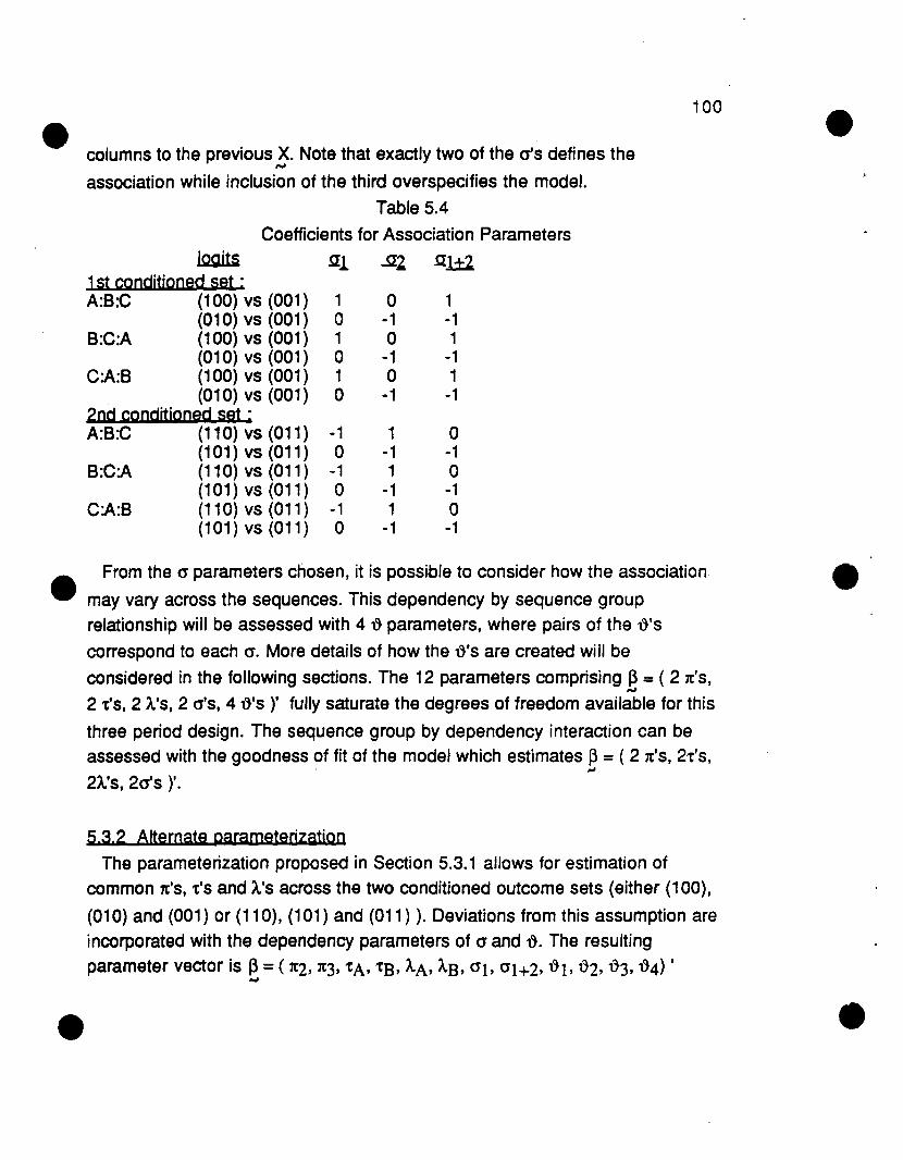
100

ecolumns to the previous X. Note that exactly two of the as defines the

f'J

association while inclusion of the third overspecifies the model.

Table 5.4

Coefficients for Association Parameters

~ !II ..,g:2 .a.l±21st conditioned set :A:B:C (100) vs (001) 1 0 1

(010) vs (001) 0 -1 -1B:C:A (100) vs (001) 1 0 1

(010) vs (001) 0 -1 -1C:A:B (100) vs (001) 1 0 1

(010) vs (001) 0 -1 -12nd conditioned set :A:B:C (110) vs (011) -1 1 0

(101) vs (011) 0 -1 -1B:C:A (110) vs (011) -1 1 0

(101) vs (011) 0 -1 -1C:A:B (110) vs (011) -1 1 0

(101) vs (011) 0 -1 -1

.. From the cr parameters chosen, it is possible to consider how the association

., may vary across the sequences. This dependency by sequence group

relationship will be assessed with 4 t} parameters, where pairs of the t}'s

correspond to each cr. More details of how the t}'s are created will be

considered in the following sections. The 12 parameters comprising 13 = ( 2 1t'S,-.J

2 t'S, 2 A'S, 2 cr's, 4 t}'s)' fully saturate the degrees of freedom available for this

three period design. The sequence group by dependency interaction can be

assessed with the goodness of fit of the model which estimates 13 = ( 2 1t'S, 2't's,...2A'S, 2cr's )'.

5,3,2 Alternate parameterization

The parameterization proposed in Section 5.3.1 allows for estimation ofcommon 1t'S, 't'S and A'S across the two conditioned outcome sets (either (100),

(010) and (001) or (110), (101) and (011) ). Deviations from this assumption are

incorporated with the dependency parameters of cr and t}. The resulting

parameter vector is 13 = ( 1t2, 1t3, 'tA, 'tB, AA, A.B, crb cr1+2, t}b t}2, t}3, t}4) ,-.J

101

An alternate and equivalent way to analyze this model is to consider a block

design structure. Each block corresponds to one of the conditioned sets and

functions to estimate the 6 parameters: 21t's, 2't's and 2A'S within each set.

0-1100-1000000

1 -1 01 1 -1 000000

0-1 -1 1 00000000

1 -1 -1 001 000000

0-10-1 -10000000

1-11-1-10000000

0000000-1100-1

000000-1 0 1 -1 -1 0

0000000-1 -1100

000000 -1 0 0 1 0-1

0000000 -1 0 -1 -1 0

000000 -1 0 -1 000

where ~s =(1t2,s1, 1t3,s1 , 'tA,s1, 'tB,s1, AA,s1' AB,s1, 1t2,s2, 1t3,s2, 'tA,s2, 'tB,s2,

AA,s2, AB,s2 )'. Therefore,

_ [ ~ 1 ~]XA -- 0 X_ _ 2

for ~s = (~1', ~2')' where ~1 = (1t2 s1, 1t3 s1, 'tA s1, 'tB s1, AA 51, AB 51)' and ~2IV ,..",., "",J , , , , , , N

=(1t2,s2, 1t3,s2, 'tA,s2, 'tB,s2, AA,s2, AB,s2 )'. This design fully saturates the

degrees of freedom available to this structure. The disadvantage of this

structure is that the simple expression for the marginal probabilities in Table 5.1

no longer applies.

102

The logits corresponding to each conditioned set, f1 and f2, respectively, have

the corresponding expected value

E.J!1 }=~1 ~1

EA{ !2 }= ~2 ~2

Thus, if all discordant sets are used together (Le. both conditioned sets ), this

can be expressed as

(5.3.2)This can be rewritten from a definitional point of view:

(5.3.3)Notice that X =[X1', X2' ]' is the original design matrix proposed in Section 5.2.- - -Instead of considering a separate set of parameters for each conditioned set, anaverage of ~1 and ~2 across the conditioned sets provides a meaningful

~ .... estimate for the six parameters. If such an averaging process involves

combining estimates of the same sign with only somewhat differing magnitude,then the average represents a fair combination. The term (~1 + ~2) /2 in the

,.J <OJ

estimated parameter structure provides estimates averaging across theconditioned set, while the (~1-~2) / 2 terms display the disparities on these

OJ ...

averages. Thus they provide a qualifying role on interpretation of averages.Therefore, the matrix UA = [Xf, -X2'l' contains the remaining six parameters

... fW _

which account for association parameters reflecting deviations in the structureassumed with X. Table 5.5 displays this UA matrix.

~ ...

103

Table 5.5UA = [ X1', -X2'l' matrix - additional columnsv ... _

~ ~~ Q'tAxs Q~ Sl~~1st conditioned set :A:B:C (100) vs (001) 0 -1 1 0 0 -1

(010) vs (001) 1 -1 0 1 1 -1B:C:A (100) vs (001) 0 -1 -1 1 0 0

(010) vs (001) 1 -1 -1 0 0 1C:A:B (100) vs (001) 0 -1 0 -1 -1 0

(010) vs (001) 1 -1 1 -1 -1 02nd conditioned set :A:B:C (110) vs (011) 0 1 -1 0 0 1

(101) vs (011) 1 0 -1 1 1 0B:C:A (110) vs (011) 0 1 1 -1 0 0

(101) vs (011) 1 0 0 -1 0 1C:A:B (110) vs (011) 0 1 0 1 1 0

(101) vs (011) 1 0 1 0 0 0

The first two columns of this can be viewed as variations on the 0' association

parameters which also correspond to period by set interactions since they are

linear combinations of those for period effects and those for 0' parameters. It is

also important to note that the first of these additional parameters, which will bereferred to as O'p2 x s' (corresponding to the period 2 effect by set effect

interaction) is orthogonal to 0'1 of Table 5.4. Let ~O'p2xs represent the coefficients

for these parameters then :

~O'P2 xs=( 0 1 0 1 0 1 0 1 0 1 0 1) 1. 3'<rI = ( 1 0 1 0 1 0 -1 0 -1 0 -1 0 )

Similarly, O'p3 x s' the second of these association parameters, is orthogonal to

0' 1+2·~o' p3 x S = ( -1 '-1 -1 -1 -1 -1 1 0 1 0 1 0 ) 1. ~o' 1+2 = ( 1 -1 1 -1 1 -1 0 -1 0 -1 0 -1 ).

Thus, either 0'1 and 0'1 +2 or O'p2 x sand O'p3 x s can be used to describe the

across-period association. The other columns of this matrix correspond to two

association parameters for treatment by conditioned set interaction and two for

carryover by conditioned set interaction. Specifically, a significant treatment by

conditioned set interaction (O'tAxs and O'tBxs) would indicate that disparities may

be evident in a comparison of treatment effects estimated separately within the

two conditioned set blocks.

104

If one determines that the lack of fit of the model is due primarily to condition

set by period interaction and not due to either of the other two pairs of

conditioned set by effect interactions, then one could simplify the model to fit

common treatment effects (and if relavent common carryover effects), One could

still allow the period effects to vary across the conditioned sets.In this case, the two (J parameters ((Jp2 x sand (Jp3 x s) incorporate a

homogeneous dependency structure across the sequences. The four remaining

degrees of freedom needed to expand to the full degrees of freedom for the

model will be referred to as t) parameters and would be the last 4 columns of U,.,(see Table 5.5). These correspond to treatment by conditioned set and

carryover by conditioned set interactions. However, any choice for U which,. v

when added to the previous columns, defines a nonsingular matrix, would

provide an adequate choice.

The choice of t) that will be used to initiate further discussion is presented in

Table 5.6. Let (Jp2 x S, (Jp3 x s and the 4 t)'s comprise the columns of ld"', The

t)1 and t)2 are the parameters corresponding to (Jp2 x s that vary by sequence

. _group and similarly t)3 and t)4 depict how (Jp3 x s varies across the sequences.

Table 5.6

Design matrix additional columns - Y'"~2x2- ~3xs 311 312 311 ~

1st conditioned set:A:B:C (100) vs (001) 0 -1 0 0 -1 0

(010) vs (001) 1 -1 1 0 -1 0B:C:A (100) vs (001) 0 -1 0 0 0 -1

(010) vs (001) 1 -1 0 1 0 -1C:A:B (100) vs (001) 0 -1 0 0 1 1

(010) vs (001) 1 -1 -1 -1 1 12nd conditioned set :A:B:C (110) vs (011) 0 1 0 0 1 0

(101) vs (011) 1 0 1 0 0 0B:C:A (110) vs (011) 0 1 0 0 0 1

(101) vs (011) 1 0 0 1 0 0C:A:B (110) vs (011) 0 1 0 0 -1 -1

(101) vs (011) 1 0 -1 -1 0 0

J"

105

~1 and ~3 provide deviation from sequences 1 vs 3 and~2 and ~4 provide

deviation comparing sequences 2 vs 3.

To implement this method with a specific example, one way to practicallyproceed would be to initially fit X = (X1', X2')' to the data. If it fits, then one would

... ""' "-#

proceed to further reduce with such hypotheses as null carryover effects.

However, if the fit of this model is not supported, then one should identify if the

lack of fit is due to conditioned set by period, by treatment or by carryoverinteractions. This can be done through:!-A by contrast matrices applied to the

appropriate components of (~1-~2) 1 2. If only period by conditon set interaction,.." -

is present, then one could fit common t and A. parameters, allow 1t to vary by

condition set and include crp2xs and crp3xs as appropriate. In the case where all

cr interactions are significant, it would still be possible to fit X=[X1', Xi]'.... .... ...combined with cr1 and cr1 +2 and the appropriate ~'s defined relative to these

cr's to vary by the sequences.

The 12 degree of freedom matrix X* = [X, U*] fully saturates the vector space.,0# ..._

Where X* is this fUlly saturated 12 by 12 design matrix, X* -1 provides the~ N

structure through which the parameters are estimated via their relationship to

the logits,.f. The ~"=~: -1 f are estimates that are implied by this full rank

model due to the equivalence of weighted least squares and maximum

likelihood in this full rank case. Thus X* -1 is as shown in Table 5.7.N

As an example, look at how the estimate of tA is calculated in terms of the

logits when all degrees of freedom are used.

tA = 1/6 [ 3 logit (91 (100)/(001) ) - 2 logit(91 (010)/(001)) +1 logit (91 (110)/(011) )

+ 2 logit (91 (1 01 )/(011))

+ 1 logit (92(010/001)) + 1 logit(92(110/011)) -1 logit(92(101/011))

-3 logit (93 (100/001)) +1 logit(93(01 0/001)) - 2 logit (93 (1101011))

- 1 logit (93 (101/011) ) }

When all other parameters have been canceled out, each of the logitscontributes a particular weighting to tAo

1/6 [ 3 (tA from logit (911)) + 1 (tA from logit (913))

+ 2 (tA from logit (914))

-1 (tA from logit (922))

-1 (tA from logit (923)

106

Table 5.7

X*·1 where X*= [X,U*] for U· of Table 5.6(X*·1 is 1/6 of the following matrix)

-3 2 0 -1 0 2 -1 -2 -1 1 2 -2

-3 1 0 -2 0 1 -2 -1 -2 2 1 -1

3 -2 0 1 -3 1 1 2 1 -1 -2 -1

0 -1 3 -1 -3 2 -1 1 2 1 -1 -2

3 0 -3 3 0 -3 3 0 0 -3 -3 3

-1 0 -1 0 -1 0 1 0 1 0 1 0

-1 1 -1 1 -1 1 0 1 0 1 0 1

-2 0 1 0 1 0 2 0 -1 0 -1 0

0 -2 0 1 0 -1 0- 2 0 -1 0 e-2 2 1 -1 1 -1 0 2 0 -1 0 -1

1 -1 -2 2 1 -1 0 -1 0 2 0 -1

107

+ 1 ('tA from logit (932))

+1 ('tA from logit (934)

='tA

or written another way :

'tA = 1/6 { [3 logit(91 (1 00/001 ))- 3 logit (93(100/001))] +

[ logit (92(010/001)) + logit (93(010/001)) ] - 2 logit (91 (010/001)) +

[ logit (91 (110/011)) + logit (92 (110/011)) ] - 2 logit (93(110/011)) +

2 logit (91 (1 01/011)) - [ logit (92(101/011)) + logit (93(101/011)) ] }

(5.3.4)

The other rows of X· -1 similarly provide expression for the other parameters in-terms of the logits.

5.3.3 Jones and Kenward tyge of association garameters

The Jones and Kenward (1989) method for the three period design will be

discussed in more detail in Chapter 8. However, at this point, it is of interest to

consider how they treat the three period design. They briefly refer to the

situation which has been developed here with dropping the concordant

observations. They consider random subject effects and their conditioned

model develops from an underlying Poisson framework. While their treatment of

this is very brief, they still define the parameters from the joint distribution and

because of their Poisson framework, they do not consider the condition sets.

More importantly, they model only period, treatment and carryover effects. They

do not discuss modeling the association parameters, CJ.

The standard model from Kenward and Jones involves all of the joint

probabiltiies, and within this framework, their CJ factors reflect the agreement

between any two of the periods. These will be extrapolated from their situation

and applied to the six conditional joint probabilities. This relationship to the

model on conditioned sets will become more obvious. For instance, they defineCJ12 as having the value = 1 if periods 1 and 2 have the same response and the

value = -1 otherwise. Similarly, CJ13 = 1 if periods 1 and 3 agree and = -1 if they

disagree while CJ23 = 1 if periods 2 and 3 agree and =-1 otherwise. These

parameters are what Jones and Kenward have proposed for the 3 period

108

design when all 8 joint probabilities are modeled. Table 5.8 shows the

coefficients associated with each of these cr parameters when one considers

just the disjoint outcomes grouped by conditioned set.

Table 5.8

Coefficients for Jones and Kenward Parameterization(100) (010) iQ.Q.1l

CJ12 -1 -1 1

CJ13 -1 1 -1

CJ23 1 -1 -1U1Ql u.o.u W.1l

CJ12 1 -1 -1

CJ13 -1 1 -1

CJ23 -1 -1 1

For anyone sequence, the logits are created as before with respect to the lastmember in each of the two conditioned sets. The parameters CJ12, CJ13 and CJ23

are denoted with the following coefficient values as they contribute additional

columns to the design matrix on these logits.

-2 0 2

-2 2 0

2 0 -2

o 2 -2

Where Xcr12 is the vector of coefficients corresponding to CJ12, and so forth, note"-

that -(XC112 + xCJ13) =xcr23; thus, a redundancy exists when the concordant.... "J _

observations are removed from the analysis. Consideration of just CJ12 and CJ13

is sufficient. Note the relationship that exists between the Jones and Kenward

parameters and those proposed in Section 5.3.2: XCJ12 =2 xCJp3 x sand xCJ13 =2~ N ~

Xcr p2 x s· Thus, these two sets of parameters span the same vector space, only,..differing by a factor of two. Since CJ12 and cr13 are in the UA vector space, they...also correspond to period by conditioned set interactions. However, they define

109

*the ~'s like the structure of U in Table 5.6. They do not address condition set by,w

treatment or conditioned set by carryover interactions.The relationship between (0'1, 0'1 +2) and (O'p2 x s, O'p3 x s) has already been

explored and an additional relating factor between these will be developed in

Section 5.3.5. Here, further attention is given to the agreement of the Jones andKenward parameters to the other sets. It can be shown that 0'12 spans the same

vector space as XM1 = [ X, 0'1, 0'1 +2], as does 0'13. This mathematical problemN

was solved by observing that an ordinary least squares regression, where 0'12

was the outcome and XM1 columns were the factors, yielded an overall R2=1.,..

Thus 0'12 is linear combination of the columns of ~M1. The same is true for 0'13.

This implies that a test of no constraint by sequence interaction (the ~'s of the

first method) is equivalent to a test of no treatment by condition set and no

carryover by condition set interactions.

5.3.4 Summary of Association Parameters

In summary, three sets of association parameters have been considered..

Those based on looking at the deviations from the equalities imposed by theconditional independence model are 0'1 and 0'1 +2 and pertain to unity for

certain odds ratios. Another corresponds to O'p2 x sand O'p3 x s which are

interpreted as a period by set interaction. These two 0' parameters differ from the

Jones and Kenward parameters (which are 0'12 and 0'13) only by a constant

factor. It has been shown that all sets span the same vector space. Thus, any of

these could be used.

From any set of association parameters, their variation across the sequences

has been incorporated in the 4 ~ parameters. In Section 5.3.2, these ~

parameters were displayed with O'p2 x sand O'p3 x s in Table 5.6 or the

alternate parameterization in Table 5.5 stressing the condition set interactions.The choice of O'p2 x sand O'p3 x s has the advantage relative to 0'1 and 0'1 +2

that the inverse of the matrix X* provides combinations of the logits that express...the parameters in meaningful terms.

In the most general case, all three methods are different. Although the methodyielding O'p2xs and O'p3xs (method 2) and the Kenward and Jones method

(method 3) share an essentially similar way of characterizing the first 2 0'

110

parameters (differing only by the factor of 2). However, they differ in

presentation of ~ parameters.

Nevertheless, on elimination of ~ parameters, the vector spaces for all three

methods are the same and those for methods 2 and 3 have essentially the

same structure or basis. Accordingly, the test statistics for elimination of the ~'s

is the same for all methods. If the ~'s can be eliminated, method 2 provides the

most straightforward way of proceeding to assess common carryover and

treatment effects. However, results of method 1 are of interest for understanding

how condition set by period interactions relate to failure of model constraints to

hold. (More on this in the following Section 5.3.5). Given elimination of the ~'S,

the statistical tests for elimination of a's from all three methods are identical

because all correspond to further simplifications to X (Le. a stepwise modeling-.J

procedure with likelihood ratio tests).

With regards to the Kenward and Jones parameterization, one conceptual

problem is that it mixes features of methods 1 and 2. Like method 2, it in a

sense, operates off of condition set by period interactions but proceeds to

interact these with sequence to produce ~'S like method 1. And like method 2,

the U =[cr, ~] structure lacks orthogonality with X. Furthermore, it does not allow~ N

for one to address condition set by treatment or by carryover interactions. Since

methods 1 and 2 are thus somewhat cleaner, they are recommended over the

Kenward and Jones parameterization. Particularly in the case where the ~'S are

significant, one has a better understanding of what is involved with methods 1

or 2.

5,3.5 Alternate Method to relate methods 1 and 2

This section further explores the relationship between the first two methods.

In general, from method 1 the structure would be

f = [~'2 ~ '2][:Iwhere U1 and U2 incorporate the a and ~ parameters, respectively for the two

"'" ""conditioned sets. Since,

111

~1'~1+~2'~2=~

~2= -~2,-1 ~1' ~1

(5.3.5)As a reasonable starting point allow U1 = X1 '.1, then U2 = [-X2']-1. Note that this

IV """" 'V f""Io.t

implies a matrix of (J and i} parameters with the following structure-3 -3 3 0 3 02 1 -2 -1 0-3o 0 0 3 -3 0

-1 -2 1 -1 3 3o 0 -3 -3 0-3

(1 /3) 2 1 1 2 -3 01 2 -1 1 -3 02 1 -2 -1 0-31 2 -1 -2 0-3

-1 -2 1 -1 3 3-2 -1 2 1 3 32 1 1 2 -3 0

Thus,

f = ~ 1 ~ 1 ' ·1 [_~s:::

X -X' -1 u_ 2 _ 2

= [ ~1 ~] [~ 1]~ ~ 2 ~2

(5.3.6)

From equation (5.3.3), the following relationship has been shown0.5 (~1 + ~2) = 0.5 (X1 -1 f1 + X2 -1 f2)

"" - ~ """ - -Substituting from equaiton (5.3.6) yields0.5 (~1 + ~2) = 0.5 [X1 -1 (X1 ~ + Xf-1 0) + X2 -1 (X2 ~ + (-X2') -1 0) ]

""'" 'V ~ "'"' _ ,.. "'"',..., """ _

A,. ,.. = ~ + 0.5 [(Xf X1) -1 + ((-X2') X2 )-1] 0"""* IV"'" .....,.", ~

(5.3.7)

112

Thus, the average of ~1 and ~2 across the conditioned sets can be expressed... oJ

as a function of ~ + 0.5 g(X) 0 where"" 'V U

= (1 /3)

1 1 -1 1 0 01 0 -1 1 0 0

-1 -1 4 2 0 31 1 2 4 -3 0o 0 0 -3 0 0o 0 3 0 0 0

Thus if the contribution of the association parameters is not too big, then theaverage is predominately based on ~.

N

One can similarly relate the other quantities with

0.5 (~1 - ~2) = 0.5 [ X1 -1 f1 - X2 -1 f2]tI\,J",.j ,.. N ~ ,..,.

(5.3.8)Thus,

This verifies what was discussed in previous sections. The null hypothesis that(~1 - ~2) / 2 = 0 is equivalent to a test of B= O. Thus tests of (J and t} from

".; /"ttl'" ~ #iJ

methods 1 and 2 have equivalent test statistics.Note this derivation is based on assuming U1 =X1' -1. However, any choice

,... ""of U1 reveals a similar expression in terms of the relationship (Only g1 (X) and

~ N

92(X) become more complicated.),..Looking at these relationships inversely so that they express the method 2

average and difference in terms of ~ and Bhinges on the fact that the inverse of'" ,...

h(X) exists. Since this is the case... B= [ h(X)) -1 (~1 - ~2)

I'tw '" """" ItJ

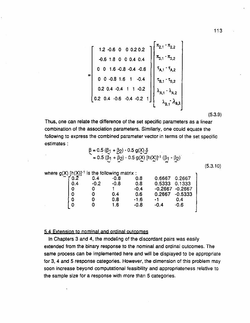
113

1.2 -0.6 0 o 0.20.21t2,1 - 1t2,2

-0.6 1.8 0 o 0.4 0.4 1t3•1 - 1t3,2

0 0 1.6 -0.8 -0.4 -0.6 'tA•1 - 'tA•2

=0 o -0.8 1.6 1 -0.4 'te,1 - 'te,2

0.2 0.4 -0.4 1 1 -0.2A.A.1 - A.A.2

0.2 0.4 -0.6 -0.4 -0.2 1Ae,t Ae.l

(5.3.9)

Thus, one can relate the difference of the set specific parameters as a linear

combination of the assoCiation parameters. Similarly, one could equate the

following to express the combined parameter vector in terms of the set specific

estimates:

(5.3.10)where g(X) [h(X)]o1 is the following matrix:

,.. O.~ 0.4 -0.8 0.80.4 -0.2 -0.8 0.8o 0 1 -0.4o 0 0.4 0.6o 0 0.8 -1.6o 0 1.6 -0.8

0.6667 0.26670.5333 0.1333-0.2667 -0.26670.2667 -0.5333-1 0.4-0.4 -0.6

5,4 Extension to nominal and ordinal outcomes

In Chapters 3 and 4, the modeling of the discordant pairs was easily

extended from the binary response to the nominal and ordinal outcomes. The

same process can be implemented here and will be displayed to be appropriate

for 3, 4 and 5 response categories. However, the dimension of this problem may

soon increase beyond computational feasibility and appropriateness relative to

the sample size for a response with more than 5 categories.

114

At each of the three periods, a subject responds with an outcome of r = 1, ...R. For the k-th subject in sequence group i, let the ordered outcome (Yi 1k, Yi2k,

Yi3k) be represented with outcomes (r1, r2, r3) denoting that period 1 had

response r1, period 2 had response r2, and period 3 had response r3. Working

with the discordant triples will exclude the concordant outcomes of (111), (222),... (RRR). Correspondingly, the data counts can be represented with ni,(r1, r2,

1'3) which is the number of patients in sequence i who responded jointly with

outcome r1 in period 1, r2 in period 2 and r3 in period 3.

To follow after the pattern proposed by Gart, a logistic model for each of the

marginals will be applied. Employing a reference cell parametrization, Table 5.9

exhibits the sUbject-specific, marginal probabilities applicable for each of the

periods. The probability in any cell is the probability that the outcome r isdiscerned in the j-th period for the i-th sequence. Observe that (R-1) 1t2's, (R-1)

1t3's, (R-1 )'tA'S, (R-1) 'tS's, (R-1) A.A'S, and (R-1) A.S'S are to be estimated. In

order for the parameters to be identifiable, 1t21 =1t31 ='tA1='tS1=A.A1=A.S1=0.

The three period nominal response crossover design with the simplest

structure is one where at each of the three periods, the subject can have the

outcome r=1, 2, or 3. Without considering the three concordant triplets, there are24 possible outcomes or combinations of (r1, r2, r3). For each of the sequences,

these responses can be grouped into 8 separate sets of three outcomes each,

where each set can be treated as an independent set of responses on which to

condition. The first six sets are grouped based on combinations of 2 period

responses of one value and one period response with another value (Le. (112),

(121) and (211) make up one group). The last two sets represent joint

responses where each of the response values appears once. Table 5.10

indicates the numerators of the conditional probabilities for each sequence by

outcome where each row represents a set of three that was conditioned on.

For the first six sets of outcomes, the following within subject effects are

cancelled out: (11(2, 2(11(2' (11(3, 2(11(3, 2(11(2 + (11(3, and (11(2 + 2(11(3,

respectively. For the last two sets, the subject effect (1k2 + (1k3 is cancelled out

in both cases. Thus, the last two sets could be treated as one set of six, since

any member of one set is interchangeable with the corresponding member of

the other set. Since the contrast (1 1 1 -1 -1 -1 ) applies to the full set of six for

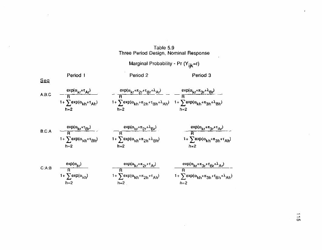
Table 5.9Three Period Design, Nominal Response

Marginal Probability - Pr (Yijk=r)

~

A:B:C

B:C:A

CAB

Period 1

exp(<Xkr+tAr)

R1+ :LeXp(<Xkh+tAh)

h=2

exp(<Xkr+tBr)

R

1+ :LeXp(<Xkh+tBh)

h=2

exp(<xkr)

R1+ :Lexp(<xkh)

h=2

Period 2

exp(<Xkr+1t2rHBr+A.Ar)R

1+ :Lexp(<Xkh+1t2h+tBh+A.Ah)

h=2

exp(<Xkr+1t2r+A.Br)

R

1+ :Lexp(<Xkh+1t2h+A.Bh)

h=2

exp(<Xkr+1t2rH Ar)

R1+ :Lexp(<Xkh+1t2hH Ah)

h=2

Period 3

exp(<Xkr+1t3r+A.Br)

R1+ :Lexp(<Xkh+1t3h+A.Bh)

h=2

exp(<Xkr+1t3r+tAr)

R1+ I,8XP(<Xkh+1t3h+tAh)

h=2

exp(<Xkr+1t3r+tBr+A.Ar)R

1+ :Lexp(<Xkh+1t3h+tBh+A.Ah)

h=2

-l.

01

116

Table 5.10Numerators of Conditional Probabilities

For three period design with A=3

!.2lll U2.ll ll1.2lA:8:C exp('tA2) exp(7t22+'t82+A.A2) exp(7t32+A.82)8:C:A exp('t82) exp(7t22+A.B2) exp(7t32+'tA2)C:A:8 exp(O) exp(7t22+'tA2) . exp(7t32+'t82

+A.A2 )

i22.ll i2..12l ~A:8:C exp(7t22+'tA2 +'tB2) exp(7t32+'tA2+A.B2) exp(7t22+7t32 +B:C:A exp(7t22+ 'tB2 +A.B2) exp(7t32+'tA2+'tB2 ) exp(7t22+ 7t32+C:A:B exp(7t22+'tA2 ) exp(7t32+'tB2 +A.A2) exp(7t22+7t32

+'tA2+t B2 +A.A2)

illll UW .u.ulA:B:C exp('tA3) exp(7t23+'tB3+A.A3) exp(1t33+A.83)B:C:A exp(tB3) exp(7t23+A.83) exp(1t33+t A3) eC:A:B exp(O) exp(7t23+tA3) exp(1t33+t 83

+A.A3 )

QW. mm. ~A:B:C exp(7t23+'tA3 +tB3) exp(7t33+'tA3+A.B3) exp(7t23+7t33+

tB3 +A.A3 +A.B3)B:C:A exp(7t23+ tB3 +A.83) exp(7t33+'tA3+'t83) exp(7t23+

7t33+tA3 +A.83)C:A:8 exp(7t23+t A3) exp(7t33+t 83 +A.A3) exp( 1t23+ 7t33

+tA3+t 83 +A.A3 )

117

Table 5.10 (cont.)Numerators of Conditional Probabilities

For three period design with R=:=3

W2l Q22l ~A:8:C exp(1t23+ 1t32+tA2+t83 exp(1t22+ 1t32+tA3+t82 exp(1t22+1t33 +tA2

+A.A3+A.82) +A.A2+A.82) +t82 +A.A2 +A.83)8:C:A exp(1t23+1t32+ tA2+t 82 exp(1t22+ 1t32+tA2+t83 exp(1t22+1t33 +'tA3

+A.83) +A.82) +'t82 +A.B2)C:A:B exp(1t23+ 1t32+'tA3+tB2 exp(1t22+ 1t32+tA2+tB2 exp(1t22+1t33 +'tA2

+A.A2) +A.A2) +'tB3 +A.A2)

(~ W2l ~A:8:C exp(1t22+ 1t33+tA3+tB2 exp(1t23+ 1t32+tA3+t83 exp(1t23+1t33 +'tA2

+A.A2+A.83) +A.A3+A.82) +'tB3 +A.A3 +A.B3)B:C:A exp(1t22+ 1t33+tA3+tB3 exp(1t23+ 1t32+'tA2+tB3 exp(1t23+1t33 +'tA3

+A.B2) +A.B3) +'tB2 +A.B3)C:A:B exp(1t22+ 1t33+tA2+'tB3 exp(1t23+ 1t32+tA3+'tB2 exp(1t23+1t33 +'tA3

+A.A3) +A.A2) +'tB3 +A.A3)

(.12.Jl !Zlli amA:B:C exp(1t22+ 1t33+tB2 exp(1t23+t A2+t B3 exp(1t32 +tA3

+A.82) +A.A2+A.B3) +A.A3)B:C:A exp(1t22+ 1t33+ tA3 exp(1t23+t B2 +A.B3) exp(1t32+t A2

+'tB3 ) +A.B2)C:A:B exp(1t22+ 1t33+tA2+tB3 exp(1t23+t A3) exp(1t32+t B2

+A.A2) +A.A3)

(.1.J2l Lilll i2.UlA:B:C exp(1t23+ 1t32+tB3 exp(1t22+t A3+t B2 exp(1t323+tA2

+A.B3) +A.A3+A.B2) +A.A2)B:C:A exp(1t23+ 1t32+ tA2 exp(1t22+t B3 +A.82) exp(1t33+t A3

+tB2 ) +A.B3)C:A:B exp(1t23+ 1t32+tA3+tB2 exp(1t22+t A2) exp(1t33+t B3

+A.A3) +A.A2)

118

(112)(122)(113)(133)(114)(144)(223)(233)(224)(244)(334)(344)(312)(213)(412)(214)

(121 )(212)(131 )(313)(141 )(414)(322)(332)(422)(422)(433)(443)(231 )(321 )(241 )(421 )

each sequence, this grouping is noninformative; thus, the separation into these

2 sets of three is a practical consideration providi.ng consistency with the other

sets and without the loss of any information.

For the 72 probabilities in Table 5.10, there are 48 logits to model the 12

parameters. For the i-th sequence, the I-th conditioned set (1=1, 2, ...8) and thep-th outcome for p=1, 2, 3, let 7tilp represent the conditional probability. Then

there are 2 logits as follows :

logit(9i11) = In (7tiI1 / 7til3 )

logit (9i12) = In (7tiI2 / 7til3 )

Table 5.11 displays the design matrix associated with these logits

Incorporation of the equal adjacent odds ratio assumption allow the response

to be considered as ordinal instead of nominal. Table 5.12 shows the designmatrix where the following assumptions are made : 7t22=7t2, 7t23=27t2, 7t32=7t3,

7t33=27t3,tA2=tA,tA3=2tA,tB2~B,tB3=2tB,AA2=AA,AA3=2AA,AB2=AB,and

AB3=2AB' Thus, a six degree of freedom test is used for goodness of fit relative

to the mod131 for nominal data.

When there are 4 possible responses at each of the three periods (R=4), there

are 64 possible combinations of joint responses, of which the 4 concordant

observations are not considered. The 60 joint outcomes are grouped into 20

sets of 3 outcomes each. For each of the 3 sequence groups, the groupings of

outcomes are shown below.Set # 1: (221 )

2: (221)3: (311)4 : (331)5: (411)6 : (441)7: (232)8: (323)9: (242)10: (424)11: (343)12 : (434)13: (123)14: (132)15: (124)16 : (142)

119

Table 5.11

Design Matrix for nominal response (R=3)

~ ~ ~ ~ IA2. IAa laz lea ~ ~ ~6.2. 1aa0 0 -1 0 1 0 0 0 0 0 -1 01 0 -1 0 0 0 1 0 1 0 -1 00 0 -1 0 -1 0 1 0 0 0 0 01 0 -1 0 -1 0 0 0 0 0 1 00 0 -1 0 0 0 -1 0 -1 0 0 01 0 -1 0 1 0 -1 0 -1 0 0 0

0 0 -1 0 1 0 0 0 -1 0 -1 0-1 0 0 0 1 0 -1 0 -1 0 0 00 0 -1 0 -1 0 1 0 0 0 0 0

-1 0 0 0 0 0 1 0 0 0 -1 00 0 -1 0 0 0 -1 0 -1 0 0 0

-1 0 0 0 -1 0 0 0 0 0 0 0

0 0 0 -1 0 1 0 0 0 0 0 -10 1 0 -1 0 0 0 1 0 1 0 -10 0 0 -1 0 -1 0 1 0 0 0 00 1 0 -1 0 -1 0 0 0 0 0 10 0 0 -1 0 0 0 -1 0 -1 0 00 1 0 -1 0 1 0 -1 0 -1 0 0

0 0 0 -1 0 1 0 0 0 -1 0 -10 -1 0 0 0 1 0 0 -1 -1 0 00 0 0 -1 0 -1 0 0 1 0 0 00 -1 0 0 0 0 0 0 1 0 0 -10 0 0 -1 0 0 0 0 -1 -1 0 00 -1 0 0 0 -1 0 0 0 0 0 0

-1 1 1 -1 0 0 -1 1 -1 1 1 -10 0 1 -1 -1 1 0 0 0 0 1 -1

-1 1 1 -1 1 -1 0 0 0 0 -1 10 0 1 -1 1 -1 -1 1 0 0 0 0

-1 1 1 -1 -1 1 1 -1 1 -1 0 00 0 1 -1 0 0 1 -1 1 -1 0 0

1 -1 0 0 -1 1 1 -1 1 -1 0 00 0 1 -1 -1 1 0 0 0 0 1 -11 -1 0 0 0 0 -1 1 0 0 1 -10 0 1 -1 1 -1 -1 1 0 0 0 01 -1 0 0 1 -1 0 0 0 0 0 00 0 1 -1 0 0 1 -1 1 -1 0 0

120

Table 5.11 (cont.)

Design Matrix for nominal response (R=3)

~ ~ ~ ~ ~ ~ ISZ IaJ ~ ~ ~a2 ~~1 0 -1 1 0 -1 1 0 1 0 -1 10 1 -1 0 1 -1 0 1 0 1 -1 01 0 -1 1 -1 1 0 0 0 0 1 00 1 -1 0 -1 0 1 -1 0 0 0 11 0 -1 1 1 0 -1 1 -1 1 0 00 1 -1 0 0 1 -1 0 -1 0 0 0

0 1 1 -1 -1 0 0 1 0 1 1 -11 0 0 -1 -1 1 1 0 1 0 0 -10 1 1 -1 1 -1 -1 0 0 0 0 11 0 0 -1 0 -1 -1 1 0 0 1 00 1 1 -1 0 1 1 -1 1 -1 0 01 0 0 -1 0 1 0 -1 0 -1 0 0

121

Table 5.12

Design Matrix for ordinal response (R=3)

1k2. lta IA 16 ~ 2..a0 -1 1 0 0 -11 -1 0 1 1 -10 -1 -1 1 0 11 -1 -1 0 0 10 -1 0 -1 -1 01 -1 1 -1 -1 0

0 -1 1 0 -1 -1-1 0 1 -1 -1 00 -1 -1 1 0 -1

-1 0 0 1 0 -10 -1 0 -1 -1 0

-1 0 -1 0 0 0

0 -2 2 0 0 -22 -2 0 2 2 -20 -2 -2 2 0 02 -2 -2 0 0 20 -2 0 -2 -2 02 -2 2 -2 -2 0

0 -2 2 0 -2 -2-2 0 2 -2 -2 00 -2 -2 2 0 0-2 0 0 2 0 -20 -2 0 -2 -2 0

-2 0 -2 0 0 0

1 -1 0 1 1 -10 -1 1 0 0 -11 -1 -1 0 0 10 -1 -1 1 0 01 -1 1 -1 -1 00 -1 0 -1 -1 0

-1 0 1 -1 -1 00 1 1 0 0 -1

-1 0 0 1 0 -10 1 -1 1 0 0

-1 0 -1 0 0 00 1 0 -1 -1 0

122

Table 5.12 (cant.)

Design Matrix for ordinal response (R=3)

Ka Ita. 18 Ie t..a ~a1 1 -2 1 1 12 -1 -1 2 2 -11 1 1 0 0 12 -1 -1 -1 0 21 1 1 1 1 02 -1 2 -1 -1 0

2 -1 -1 2 2 -11 -2 1 1 1 -22 -1 -1 -1 0 21 -2 -2 1 0 12 -1 2 -1 -1 01 -2 2 -2 -2 0

17:18 :19 :20 :

(134)(143)(234)(243)

(341 )(431 )(342)(432)

(413)(314)(423)(324)

123

As was the case with the R=3 response situation, these sets are grouped

based on the value of the subject effect that is cancelled out. Also, the last 8 sets

of 3 could equivalently be grouped as 4 sets of 6. Implementing this, however,

requires computer software dealing simultaneously with 12 groups with 3

outcomes and 4 groups with 6 outcomes.

For each of the sequences there are 40 logits to consider where the third

triple will be considered the reference cell. For the ordinal response, with an

equal adjacent odds ratio model, Table 5.13 displays the design matrix. Withthis assumption 1t22=1t2, 1t23=21t2, and 1t24=31t2. Similar relationships exist for

the other parameters, reducing the number of parameters from 18 to 6.

For the response with 5 possible ordinal values, the 120 discordant joint

outcomes can similarly be grouped as above into 40 sets of 3, for each of thesequences. Thus, maximum likelihood techniques can be used to estimate 1t2,

1t3, 'tA, 'tB, A.A' and A.B where an equal adjacent odds ratio model has been

presumed. This modeling can be done relative to the 80 logits available at each

sequence.

At this point, a word about missing data is of interest. For an investigator to

consider a design where the outcome has a 4 or 5 category response, there

should be at least a moderate sample size to support these categories. Still not

all of the possible trichotomies will be observed across the three periods. The

methods proposed in this section are still applicable. If an entire set of 3 triples

is unobserved, then the corresponding logits are not considered, thus deleting

the corresponding rows of the design matrix. However, subjects with data

missing for one or more periods cannot be included in this analysis as there is

no provision for a subset of responses corresponding to nonmissing periods.

This issue is discussed later.

124

Table 5.13Design Matrix for Ordinal Response (R=4)

.sm ~ lka IA Ia ~ ~

1 .0 -1 1 0 0 -11 -1 0 1 1 -10 -1 -1 1 0 01 -1 -1 0 0 10 -1 0 -1 -1 01 -1 1 -1 -1 0

2 0 -1 1 0 -1 -1-1 0 1 -1 -1 00 -1 -1 1 0 0

-1 0 0 1 0 -10 -1 0 -1 -1 0

-1 0 -1 0 0 0

3 0 -2 2 0 0 -22 -2 0 2 2 -20 -2 -2 2 0 02 -2 -2 0 0 2 e0 -2 0 -2 -2 02 -2 2 -2 -2 0

4 .0 -2 .2 .0 -2 -2-2 0 2 -2 -2 00 -2 -2 2 0 0-2 0 0 2 0 -20 -2 0 -2 -2 0

-2 0 -2 0 0 0

5 0 -3 3 0 0 -33 -3 0 3 3 -30 -3 -3 3 0 03 -3 -3 0 0 30 -3 0 -3 -3 03 -3 0 -3 -3 0

6 0 -3 3 0 -3 -3-3 0 3 -3 -3 00 -3 -3 3 0 0

-3 0 0 3 0 -30 -3 0 -3 -3 0

-3 0 -3 0 0 0

125

Table 5.13 (cant.)Design Matrix for Ordinal Response (R=4)

~ ~ ~ IA Ie AA ~B.7 1 -1 0 1 1 -1

0 -1 1 0 0 -11 -1 -1 0 0 10 -1 -1 1 0 01 -1 1 -1 -1 00 -1 0 -1 -1 0

8 -1 0 1 -1 -1 00 1 1 0 0 -1

-1 0 0 1 0 -10 1 -1 0 0 0

-1 0 -1 0 0 00 1 0 -1 -1 0

9 2 -2 0 2 2 -20 -2 2 0 0 -22 -2 -2 0 0 20 -2 -2 2 0 02 -2 2 -2 -2 00 -2 0 -2 -2 0

10 -2 0 2 -2 -2 00 2 2 0 0 -2

-2 0 0 2 0 -20 2 -2 2 0 0

-2 0 -2 0 0 00 2 0 -2 -2 0

11 1 -1 0 1 1 -10 -1 1 0 0 -11 -1 -1 0 0 10 -1 -1 1 0 01 -1 1 -1 -1 00 -1 0 -1 -1 0

12 -1 0 1 -1 -1 00 1 1 0 0 -1

-1 0 0 1 0 -10 1 -1 1 0 0

-1 0 -1 0 0 00 1 0 -1 -1 0

126

Table 5.13 (cont)Design Matrix for Ordinal Response (R=4)

.sm. ~ xa IA 1a ~ ~a13 . 1 1 -2 1 1 1

2 -1 -1 2 2 -11 1 1 0 0 12 -1 -1 -1 0 21 1 1 1 1 02 -1 2 -1 -1 0

14 2 -1 -1 2 2 -11 -2 1 1 1 -22 -1 -1 -1 0 21 -2 -2 1 0 12 -1 2 -2 -2 01 -2 2 -2 -2 0

15 1 2 -3 1 1 23 -1 -2 3 3 -11 2 2 0 0 1 e3 -1 -1 -2 0 31 2 1 2 2 03 -1 3 -1 -1 0

16 3 -2 -1 3 3 -21 -3 2 1 1 -3

.3 -2 -2 -1 0 31 -3 -3 2 0 13 -2 3 -2 -2 01 -3 3 -3 -3 0

17 2 1 -3 2 2 13 -2 -1 3 2 -22 1 1 0 0 23 -2 -2 -1 0 32 1 2 1 1 03 -2 3 -2 -2 0

18 3 -1 -2 3 3 -12 -3 1 2 2 -33 -1 -1 -2 0 32 -3 -3 1 0 23 -1 3 -1 -1 02 -3 3 -3 -3 0

127

Table 5.13 (cont)Design Matrix for Ordinal Response (R=4)

~ ~ ~ 1A Ia ~ la19 1 1 -2 0 -1 1

2 -1 -1 1 2 -11 1 1 0 0 12 -1 -1 1 0 21 1 1 1 1 02 -1 2 -1 -1 0

20 2 -1 -1 0 2 11 -2 1 -1 1 -22 -1 -1 0 0 21 -2 -2 2 0 12 -1 2 -1 -1 01 -2 1 -2 -2 0

128

5,5 Logistic Model for Binary Response with two Latin sQuares

A three period, three treatment crossover design with two Latin squares

involves the 6 sequences ( A:B:C, B:C:A, C:A:B, A:C:B, C:B:A, and B:A:C).

Consider the outcome to be a binary response, then the marginal probabilities

are arrived at as they were in Table 5.1. Table 5.14 displays the marginal

probabilities for the three additional sequences of A:C:B, C:B:A, and B:A:C and

this table augmented to Table 5.1 provides the appropriate probabilities for all

six sequences.

SeQuenceA:C:B

C:B:A

C:A:B

Period1

2

3

1

2

3

1

2

3

Table 5.14Marginal Probabilities = Pr (Yijk=1)

Probability

exp(Clk + 'tA) / (1 + exp(Clk + 'tA)

exp(cxk + 1t2 + AA) / 1 + exp( cxk + 1t2 + AA)

exp(cxk + 1t3 + 'tB) / 1 + exp( cxk + 1t3 + tB )

exp(cxk) / (1 + exp(cxk)

exp(cxk + 1t2 + tB) / 1 + exp( cxk + 1t2 + tB)

exp(cxk + 1t3 + 'tA + AB) /1 +exp( cxk + 7t3 + tA + AB)

exp(cxk + tB )- / (1 + exp(cxk + tB )

exp(cxk + 1t2 + 'tA + AB ) / 1 +exp(cxk + 1t2 + tA + AB )

exp(cxk + 1t3 + AA) / 1 + exp( cxk + 1t3 + AA)

The steps to arrive at the logits on which model analysis is made are the same

as those presented in section 5,2. There are 24 logits across the 6 sequences

(4 logits per sequence, 2 for each conditioned set) on which 6 parameters can

be estimated. As has been previously shown, not only does each Latin square

provide sufficient estimability of the six parameters, but each conditioned set of

3 within the Latin square also allows estimation. Table 5.15 displays the

associated logits and design matrix rows for the second Latin square.

Appending these rows vertically to the rows of Table 5.3 yields the full design

matrix for all 6 sequences.

129

Table 5.15

Logits and design matrix for second Latin square~ design matrix (Xl

1st conditioned set :A:C:B (100) vs (001) -1t3 + tA - tB 0-1 1 -1 0 0

(010rvs (001) 1t2 - 1t3 + tB - AA 1 -1 0 1 -1 0

C:B:A (100) vs (001) -1t3 - tA - AB 0-1 -1 0 0 -1

(010) vs (001) 1t2 -1t3 - tA + tB - AB 1 -1 -1 1 0 -1

B:A:C (100) vs (001) -1t3 + tB - AA 0-1 o 1 -1 0(010) vs (001) 1t2 - 1t3 + t A - AA + AB 1 -1 1 0 -1 1

2nd conditioned set :A:C:B (110) vs (011) -1t3 + tA - tB 0-1 1 -1 0 0

(101) vs (011) -1t2 + tA - tB + AA -1 0 1 -1 1 0

C:B:A (110) vs (011) -1t3 - tA - AB 0-1 -1 0 0 -1

(101) vs (011) -1t2 - tB -1 0 0 -1 0 0

B:A:C (110)vs (011) -1t3 + tB - AA o -1 0 1 -1 0(101) vs (011) -1t2 - t A + tB - AB -1 0-1 1 0 -1

Incorporating the second Latin square into the design, thus produces a more

efficient estimate of parameters, where the parameters are assumed to have

common values across Latin square and sets of conditioned outcomes.

If instead, one wishes to consider different parameters for the Latin square,

then 12 parameters could be considered as

~s =(1t2,L1, 1t3,L1, tA,L1, tB,L1, AA,L1, AB,L1, 1t2,L2, 1t3,L2, tA,L2, tB,L2,N

AA,L2, AB,L2 )'.

The design matrix would exhibit the following block design structure as shown

below

X = I~ l1 ~ 12 x6]

.~ ~ 12 x6 ~ l2

where XL1 is the design matrix in Table 5.3, XL2 is the design matrix of Table~ N

5.14 and 0 12 x 6 is a 12 by 6 matrix of zeros. These parameters allow-consideration of interactions of effect (either period, treatment or carryover) by

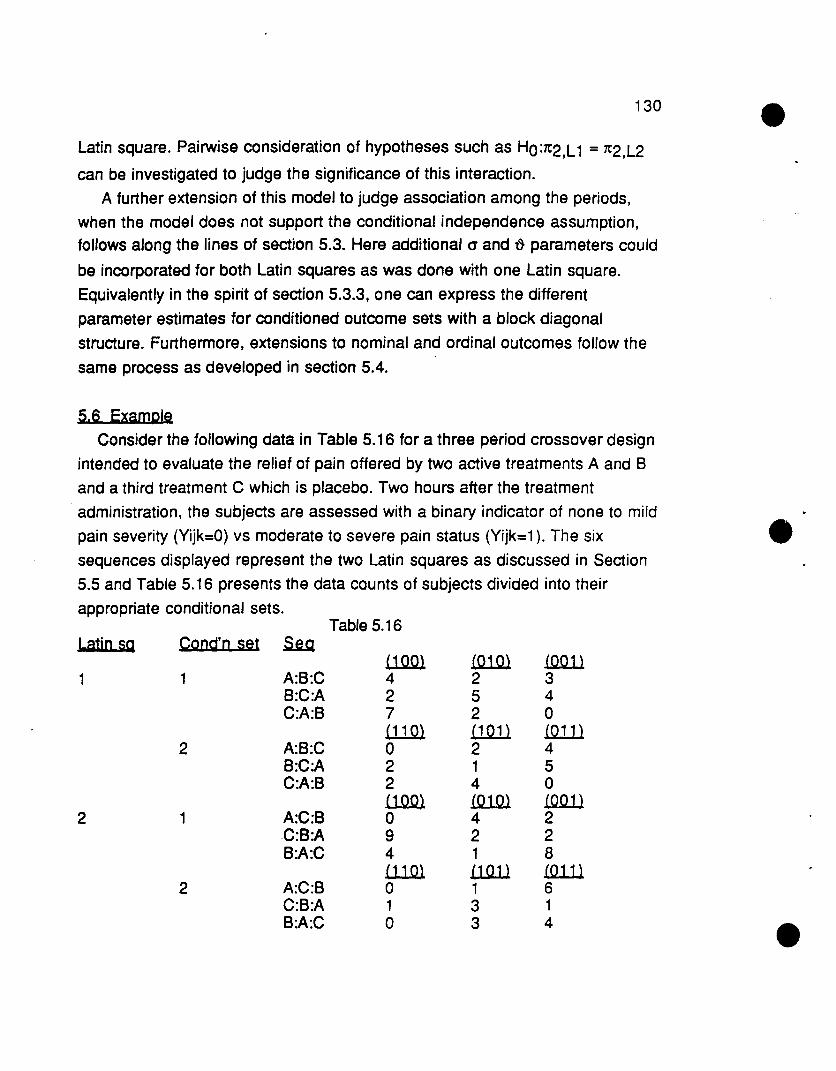
130

Latin square. Pairwise consideration of hypotheses such as HO:1t2,L1 = 1t2,L2

can be investigated to judge the significance of this interaction.

A further extension of this model to judge association among the periods,

when the model does not support the conditional independence assumption,

follows along the lines of section 5.3. Here additional a and ~ parameters could

be incorporated for both Latin squares as was done with one Latin square.

Equivalently in the spirit of section 5.3.3, one can express the different

parameter estimates for conditioned outcome sets with a block diagonal

structure. Furthermore, extensions to nominal and ordinal outcomes follow the

same process as developed in section 5.4.

5.6 Example

Consider the following data in Table 5.16 for a three period crossover design

intended to evaluate the relief of pain offered by two active treatments A and 8

and a third treatment C which is placebo. Two hours after the treatment

administration, the subjects are assessed with a binary indicator of none to mild

pain severity (Yijk=O) vs moderate to severe pain status (Yijk=1). The six

sequences displayed represent the two Latin squares as discussed in Section

5.5 and Table 5.16 presents the data counts of subjects divided into their

appropriate conditional sets.

Latin SQ

1

2

Cond'n set

1

2

1

2

Table 5.16S§.g

WlO.l !O.1O.l !.Q.QllA:8:C 4 2 38:C:A 2 5 4C:A:B 7 2 0

ll1Ql Lllill m.wA:B:C 0 2 4B:C:A 2 1 5C:A:B 2 4 0

WlO.l LQ1Q1 .LQQ.1.lA:C:B 0 4 2C:B:A 9 2 2B:A:C 4 1 8

U1Ql i1Q.ll lQ11.lA:C:B 0 1 6C:B:A 1 3 1B:A:C 0 3 4

131

First, a block d~sign matrix will be considered which allows for the interaction

of the Latin square effect with the period, treatment and carryover effects. Thusfor XL1 the design matrix in Table 5.3 for the first Latin square and XL2 the

~ ~

design matrix in Table 5.13 for the second Latin square, this model is :

X = [ ~ L1 ~ 12 x6 ]

- ~ 12 x6 ~ L2

The associated parameter vector is ~s = (1t2,L1, 1t3,L1, tA,L1, tB,L1, AA,L1,

AB,L1, 1t2,L2, 1t3,L2, 'tA,L2, tB,L2, AA,L2' AB,L2 )'. The goodness of fit of this

model, as evaluated with the likelihood ratio statistic with 12 degrees of

freedom, is 20.16 (p-value=0.06). Maximum likelihood estimates of this log

linear model are compared across the parameters with appropriate chi-square

statistics for tests of contrasts relative to the design matrix. Although this model

provides a rough fit, the parameters correspondingly compared across Latin

square designs are statistically equivalent. Thus, all of the following hypothesesof non-significant interaction are supported: 1t2,L1=1t2,L2, 1t3,L1=1t3,L2,

tA,L1='tA,L2, tB,L1=tB,L2, AA,L1=AA,L2, and AB,L1=AB,L2·

The model of interest implied by these restriction focuses on the 24 by 6

design matrix where the matrix of Table 5.15 is appended vertically after the

design matrix of Table 5.3. Therefore, the two period, two treatment and two

carryover effects are estimated as common across the two Latin squares. The

goodness of fit of this model is not sufficient to support the Gart type of

assumption of conditional independence extended to this three period design

(X2=31.32, df=18, p-value=0.027). As discussed in Section 5.3.1, the inclusion

of the two °parameters provides additional columns of the design matrix that

evaluate where the deviation from this assumption appears. By the first methodof Section 5.3.1 , the first parameter 01 includes the contrast for the deviation

from the assumption that the first and third logits within each sequence areequivalent. The second 01 +2 association allows for the variation of odds of

(10/01) for period 1 and 2 as it varies for period 3.

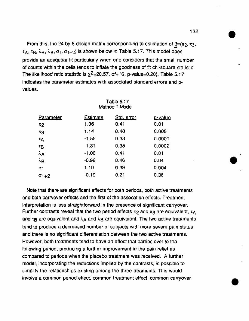
132

From this, the 24 by 8 design matrix corresponding to estimation of /3=(1t2, 1t3,#OJ

tA, tB, A.A, A.B, (11, (11+2) is shown below in Table 5.17. This model does

provide an adequate fit particularly when one considers that the small number

of counts within the cells tends to inflate the goodness of fit chi-square statistic.

The likelihood ratio statistic is X2=20.57, df=16, p-value=0.20). Table 5.17

indicates the parameter estimates with associated standard errors and p

values.

Table 5.17Method 1 Model

parameter Estimate Std. error p-yalue

1t2 1.06 0.41 0.01

1t3 1.14 0.40 0.005

tA -1.55 0.33 0.0001

ts -1.31 0.35 0.0002

A.A -1.06 0.41 0.01

AS -0.96 0.46 0.04 e(11 1.10 0.39 0.004

(11+2 -0.19 0.21 0.36

Note that there are significant effects for both periods, both active treatments

and both carryover effects and the first of the assocation effects. Treatment

interpretation is less straightforward in the presence of significant carryover.Further contrasts reveal that the two period effects 1t2 and 1t3 are equivalent, tAand ts are equivalent and A.A and AS are equivalent. The two active treatments

tend to produce a decreased number of subjects with more severe pain status

and there is no significant differentiation between the two active treatments.

However, both treatments tend to have an effect that carries over to the

following period, producing a further improvement in the pain relief as

compared to periods when the placebo treatment was received. A further

model, incorporating the reductions implied by the contrasts, is possible to

simplify the relationships existing among the three treaments. This would

involve a common period effect, common treatment effect, common carryover

133

effect and the first of the association parameters. Table 5.18 presents these

results. Notice the significant period effect, treatment and carryover effects

relative to placebo.

To compare these method 1 results, consider the parameter estimates frommethod 2. Here, one must first investigate the additional columns of UA =(X1', -

N ,..

X2' )' to verify whether the lack of fit of the model is due to interactions of,..conditioned set by period, by treatment or by carryover. Table 5.19 summarizesthis. Thus only 0p3xs is a significant association contribution. This conclusion

and the previous results allows one to implement a reduced structure of design

where there are common period, treatment and carryover effects for each of theconditioned sets, and including only ° p3xs. Tests from this model reveal that it

is feasible to combine the period, treatment and carryover effects across the

conditioned set, thus producing a final model comparable to that in Table 5.18.

See Table 5.20. The model from method 1 and 2 differ only by slight parameter

values but agree in magnitude, direction and significance.

Referring again to Table 5.19, notice what the Kenward and Jones estimatesare for their 013 and 012 and variations of these by the sequence group (~'s).

While 012 is significnat, as one would expect since x012 = 2 xop3xs, ~3 and ~4,., ,..

are also significant, producing difficulty in interpretation relative to the results

presented.

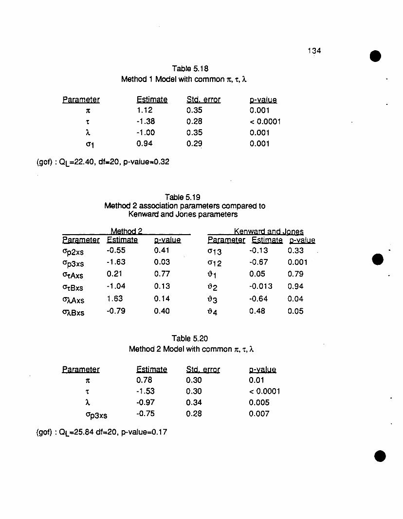
Table 5.18Method 1 Model with common 1t, t, A.

134

Parameter

1t

t

A.<11

Estimate1.12

-1.38

-1.00

0.94

Std. error0.3S

0.28

0.35

0.29

p-value0.001

< 0.0001

0.001

0.001

(got) : QL=22.40, dt=20, p-value=0.32

Table 5.19Method 2 association parameters compared to

Kenward and Jones parameters

Method 2 Kenward and JonesParameter Estimate p-yalue Parameter Estimate p-yalue

<1p2xs -0.55 0.41 <113 -0.13 0.33

<1p3xs -1.63 0.03 <112 -0.67 0.001

<1tAxs 0.21 0.77 ~1 0.05 0.79

<1tBxs -1.04 0.13 ~2 -0.013 0.94

<JAAxs 1.63 0.14 ~3 -0.64 0.04

<JABxs -0.79 0.40 ~4 0.48 0.05

Table 5.20Method 2 Model with common 1t, t, A.

Parameter

1t

t

A.

<1p3xs

Estimate0.78

-1.53

-0.97

-0.75

Std. error

0.30

0.30

0.34

0.28

p-yalue0.01

< 0.0001

0.005

0.007

(got) : QL=25.84 dt=20, p-value=0.17

135

CHAPTER 6

LOGISTIC MODELS FOR FOUR PERIOD CROSSOVER DESIGNS

FOCUSING ON DISCORDANT JOINT OUTCOMES

6.1 Introduction

The development of Chapter 6 is similar to the previous chapters on two and

three period crossover designs. Now the emphasis will be on those designs

with four periods for evaluating the effectiveness of two or more treatments.

Defining the parameters in terms of the marginal probabilities and combining

the joint outcomes into sets so as to cancel out the intersubject effects will still

be the strategy for model formulation.

Four period designs do, of course, provide great flexibility in how treatments

are administered. Two or more treatments can be considered in a variety of

sequences, regardless of whether the treatment is an active drug or a placebo.

The methods presented here are applicable for any of these combinations and

for both binary and ordinal responses. This chapter describes the four period

design with a binary outcome. It presents a basic approach to define the

appropriate design matrix. However, a general structure for multi period

designs will be developed through the extended Gart framework for P periods

and responses with R outcomes. Thus, formulation of an appropriate design

matrix for the parameters of interest for the general crossover design is

available. An important feature of the four period designs not present in two and

three period designs is the unequal number of members in the conditioned sets.

Two strategies will be proposed to analyze this framework. The first will focus on

a separate model for each conditioned set, whereby the resulting parameters

are assessed across the conditioned sets via a weighted regression. The other

strategy proposes a general log-linear model to handle the multinomial

distribution with response vectors of unequal length.

136

Section 6.2 will indicate the parameters relative to the marginal distribution

and proceed to organize the joint probabilities into conditioned sets. One

method proposed to analyze this situation will consist of two steps and is

presented in Section 6.3. In the first step, the parameters are estimated for each

conditioned set. Next these estimates are combined across the conditioned sets

to compare the estimates with weighted least squares analysis. Section 6.4

identifies another method to analyze the four period crossover design where

there are a varying number of members in the conditioned sets. This method

will focus on a multinomial model where there are varying length response

vectors. Section 6.5 relates this specifically back to the four period design.

When this model does not provide significant goodness of fit, an extension from

this basic model is suggested in Section 6.6 for evaluation. Its nature is like

counterparts in Chapters 3 ad 5 and so involves association association

parameters. Section 6.7 compares these association parameters to those

provided by Jones and Kenward(1989). Section 6.8 deals with the case of

nominal and ordinal responses. An example to illustrate these methods follows

in Section 6.9.

6.2 Conditional logistic model for binary response

Consider the four period crossover design with a binary response observed at

each of the four periods. For the most general case, assume that there are four

treatment sequences described as follows: A:B:C:D, B:C:D:A, C:D:A:B and

D:A:B:C. This particular treatment structure represents one Latin square. Other

Latin square designs are available by themselves or in conjunction with the one

exemplified here. The methods and strategies presented below are also

applicable for any other variety of sequences with two or more treatments. Thebinary response Yijk, taking values a and 1, is specific to the k-th subject in the

i-th sequence group and for the j-th period. The profile (Yi1 k, Yi2k, Yi3k, Yj4k)

represents the joint outcome vector. Of this set, responses (0000) and (1111)

are not considered in this conditional set analysis in that they contribute no

discriminating information with respect to treatment response.

137

Parameter structure for the proposed log-linear model will have definitions

relative to the marginal probabilities. Based on a reference cell coding scheme,

the parameters have the following interpretation :

uk = the within subject probability for the k-th subject

1tj = the j-th period effect

th = h-th treatment effect for h=A, B, C or 0

Ah = carryover effect for the h-th treatment

" In order to eliminate redundancies for estimation purposes, it is necessary toassume that 1t1 =tD=AD=O and this convention will be reflected in Table 6.1.

The uk, which reflect intersubject variability, will be canceled out in the resulting

conditioning. Thus, for the resulting intrasubject analysis, they can be fixed or

random effects.

SeQuenceA:B:C:D

B:C:D:A

C:D:A:B

D:A:B:C

Period1

2

3

4

1

23

4

1

2

3

4

1

2

34

Table 6.1

Marginal Probabilities = Pr (Yijk=1)

Marginal Probabilities

exp(uk"+ tA) / (1 + exp(uk+ tA) )

exp(uk + 1t2 + tB+ AA) / (1 + exp( uk + 1t2 + tB+ AA ) )

exp(uk + 1t3 + tC+ AB) / (1 + exp( uk + 1t3 + tC+ AB ) )

exp(uk + 1t4 + AC) / (1 + exp( uk + 1t4 + AC ) )

exp(uk + tB) / (1 + exp(Uk+ tB) )


exp(uk + 1t3 + Ac) / (1 + exp( uk + 1t3 + Ac ) )exp(uk + 1t4 + tA) / (1 + exp( uk + 1t4 + tA ) )

exp(uk + "tC) / (1 + exp(uk+ tC) )

exp(uk + 1t2 + AC) / (1 + exp( uk + 1t2 + AC ) )

exp(uk + 1t3 + tA) / (1 + exp( uk + 1t3 + tA ) )


exp(uk) / (1 + exp(uk) )

exp(uk + 1t2+ tA) / (1 + exp( uk + 1t2 + tA ) )



138

There are 16 possible joint outcomes for the four period, binary response

crossover design of which 14 represent discordant outcomes essential to the

modeling. There are three conditioned sets to partition these responses into. Let

h index these sets where h=1, 2, ...H. For the four period design H=3. The first

of these sets is made up of the outcomes (1000), (0100), (0010) and (0001).

The conditional probabilities of anyone of these outcomes conditional on theother 4 outcomes results in the canceling of the term exp(cxk). The other two

conditioned sets are distinguished from this set with respect to the function of

the intersubject variability that is canceled out. For the set (1100), (1010),(1001), (0110), (0101) and (0011), the term exp(2cxk) is a common element. The

final set has exp(3cxk) as the common term to be factored out and its members

are (1110), (1101), (1011) and (0111). Therefore, members of the conditioned

sets are distinguished by the number of positive responses that occur over the

four periods of observation.

One of the conditional probabilities for the sequence A:S:C:D will be worked

out in detail. Others follow suit with similar derivation. The subject specific

denominator for the joint probability is :91 (CX,1t,'t,A) =

(1 + exp(cxk +'tA) ) * (1 + exp(cxk + 1t2 + 'tS +AA) ) * (1 + exp(cxk +1t3 + 'tC+ AS))

* (1 + exp(CXk + 1t4 + A.c) )Also lets1 ( Cl,1t,t,A) =

[ exp(cxk+'tA) +exp( CXk+1t2+'tS+AA) + exp( CXk+1t3+'tC+AS) + exp( CXk+1t4+A.c)]

Then

Pr [ (1000) I (1000), (0100), (0010) or (0001)] =[ exp(cxk + 'tA) / 91 (CX,1t,'t,A)] / [S1 (CX,1t,'t,A) / 91 (CX,1t,'t,A) ]

= exp('tA) / [exp( 'tA) + exp( 1t2 + 'tS + AA) + exp( 1t3 + AS)]

(6.2.1 )

Table 6.2 displays the numerators of the conditional probabilities for the four

sequence groups and for all members of the three conditioned sets.

Table 6.2Four Period Binary Design


~

(1000) (0100) (0010) (0001 )

A:B:C:D exp(tA} exp(7t2H B+A.A} exp(7t3H C+A.B} exp(7t4+A.c}

B:C:D:A exp(tB} exp( 7t2H C+A.s) exp(7t3+A.c') exp(7t4H A}

C:D:A:S exp(tc) exp(7t2+A.C) exp(7t3H A) exp(7t4H S+A.A)

D:A:S:C exp(o} exp(7t2H A) exp(7t3HS+A.A) exp(7t4H C+A.B}

(110m (1010) (1001\ (0110)

A:B:C:D exp(7t2H AHB+A.A) exp(7t3H AHC+A.S} exp(7t4H A+A.C} exp(7t2+7t3+tBHC+A.A+A.B)

B:C:D:A exp(7t2H BHC+A.S} exp(7t3H S+A.C) exp(7t4H AH S) exp(7t2+7t3+tC+A.S+A.C}

C:D:A:S exp(7t2+'tC+A.C) exp(ll:3 H AHC) exp(ll:4H SH C+A.A) exp(ll:2+ll:3+tA+AC)

D:A:S:C exp(7t2+'tA) exp(ll:3H S+AA) eXp(7t4H C+As} exp(7t2+ll:3+tAHS+A.A}

-"

<.u(£)

Table 6.2 (continued)Four Period Binary Design


~

(0101 ) (0011 )A:S:C:D (con'l) exp(1t2+1t4+'tS+AA+AC} exp(1t3+1t4+'tC+AS+AC}

S:C:D:A exp(1t2+1t4+'tA+tC+As } exp(1t3+1t4+'tA+AC}

C:D:A:S exp(1t2+1t4+'tS+AA+AC} exp(1t3+1t4+'tA+'tS+AA}

D:A:S:C exp(1t2+1t4+'tA+tC+AS) exp(1t3+1t4+'tS+'tC+AA+AS)

(1110) (llQl) (lOll) (Q111)A:S:C:D exp(1t2+1t3+'tA+'ts+tC+AA+AS} exp(1t2+1t4+'tA+'tS+AA+AC} exp(1t3+1t4+'tA+tC+As+AC} exp(1t2+1t3+1t4+1S+1C+AA+As+AC}

S:C:D:A exp(1t2+1t3+'tS+tC+As+Ac} exp(1t2+1t4+'tA+'tS+'tC+AS} exp(1t3+1t4+'tA+tS+AC) exp(1t2+1t3+1t4+'tA+'tc+As+Ac )

C:D:A:S exp(1t2+1t3+'tA+tC+AC} exp(1t2+1t4+'tS+'tC+AA+AC) exp(1t3+1t4+'tA+tS+tC+AA) exp(1t2+1t3+1t4+'tA+'tS+AA+AC}

D:A:S:C exp(1t2+1t3+'tA+tS+AA) exp(1t2+1t4+'tA+tC+1..s) exp(1t3+1t4+tS+'tC+AA+1..S) exp(1t2+1t3+1t4+1A+'tS+'tC+AA+1..S)

~

o

e e e

141

The partition of the joint outcomes into these conditioned sets results in sets

that have an unequal number of members. This presents a problem with the

type of analysis presented so far in Chapters 3, 4 and 5, because there are

unequal numbers of /ogits within each set. The following sections will present

two viable methods for dealing with this dilemma. Each of these approaches

consider the 11 logits for each sequence groups; 3 logits for the first conditioned

set,S for the second set and 3 logits for the final set. For the i-th sequence

group, these logits have the following expressions in terms of the conditionalprobabilities, 1tj( ).

logit (8i1) =In ( 1tj (1000) /1tj (0001) )

logit (8i2) =In ( 1tj (0100) /1tj (0001) )

logit (8j3) =In ( 1tj (0100) /1tj (0001) )

logit (8i4) =In ( 1tj (1100) /1tj (0011) )

logit (8iS) = In (1tj (1010) /1tj (0011))

logit (8i6) = In ( 1tj (1001) / 1tj (0011) )

logit (8i7) =In ( 1ti (0101) /1tj (0011) )

logit (8iS) = I.n ( 1tj (0011) /1tj (0011) )

logit (8i9) = In (1tj (1110) / 1tj (0111))

logit (8i,1 0) =In ( 1ti (1101) / 1ti (0111) )

/ogit (8i, 11) =In ( 1ti (1011) / 1ti (0111) )(6.2.2)

6.3 Two-stage strategy

The strategy described in this section has two components. First estimates of

the parameters are generated separately for each conditioned set. Then they

are compared and combined across these sets. Modeling of common period,

treatment and carryover effects is possible as well as investigation of other

relevant relationships. Estimated parameters can uniquely be realized from any

one of the conditioned sets. For instance, for the first conditioned set and the

first three sequences (A:8:C:D, 8:C:D:A, C:D:A:8), the nine logits for the nineparameters (31t's, 3t's, 3)..'s) produce a design matrix that is nonsingular. No

redundancy exists in estimating the 9 parameters from the first three sequences

of the first conditioned set. Therefore, adding the fourth sequence within this set

provides additional information but it is not necessary for estimation of the

142

parameters. Furthermore, the second conditioned set alone is sufficient to

estimate the parameters, as is the third set.

Three separate log-linear models can be appraised relative to the 3, 5 and 3

logits, respectively for the conditioned sets. For each set, the underlying

probability model is based on a multinomial distribution where each sequence

is assumed to arise from this distribution with 4, 6 and 4 multinomial responses,respectively. In each case the maximum likelihood estimates are f3h, which

have dimension 9 by 1. For the specific design being discussed, the goodness

of fit is assessed with 3, 11 and 3 degrees of freedom, respectively. Nine of

these 17 degrees of freedom pertain to second order carryover effects, three for

each of the models. The other eight degrees of freedom for the second model

relate to constraints of association. The design matrix for each of the models to

estimate the nine parameters is shown in Table 6.3 where the rows correspond

to the appropriate conditioned set.Given these f3h and the associated COV(f3h), weighted least squares analysis

can be performed to compare these estimates. Of initial interest, the hypothesis

to compare the three second period effects across the conditioned sets is a two

degree of freedom test where HO: 1t2,h=1 = 1t2,h=2 = 1t2,h=3. Similar tests are

available for the other 8 effects. Subsequent to the potential simplifications

implied by these comparisons, one can produce a more parsimonious design to

assess the contribution of period, treatment and carryover effects with common

parameters for the respective conditioned sets. Such hypotheses further

address goodness of fit. Note that there are 18 degrees of freedom for

equivalence of parameters across the sets. This 18 degree of freedom

contribution to homogeneity of fit along with the 17 (3 + 11 + 3) degrees of

freedom for goodness of fit in the first stage of analysis allows for 35 total

degrees of freedom devoted to fit of the model. The remaining degrees of

freedom are the 9 parameters that are estimated against the 44 functions

available.

6.4 Log-Ijnear model for multinomial with varying response vectors

The display of the conditional probabilities in Table 6.2 calls for the

development of theory to handle the situation where subpopulations (in this

143

case conditioned sets by sequence profile) have different numbers of a priori

defined responses. Standard theory for the log-linear model, where the

assumption of an underlying multinomial distribution is made, is based on the

assumption of r response categories for each subpopulation. However, for the

four period design, one needs to recognize that the subpopulations comprising

the first conditioned set have four responses, the second set includes six

responses, while the third set has four possible categories of response. The

following theory develops the structure necessary to include the varying number

of outcomes with multinomial probabilities.

The discussion is concerned with developing a log-linear model with

maximum likelihood estimates when the response vectors have varying lengths.

Such a situation arises with the 4 period crossover design where the three

conditioned sets have 4, 6 and 4 members, respectively. Additionally, this

modeling will be shown to be of further interest when there are subjects from the

crossover study who have missing data for some of the periods. Thus, the

information from the observed subset of periods can be used concurrently with

the full set of joint responses.

Let the count corresponding to the i-th sequence, the h-th conditioned set andthe I-th member be denoted as nihl. The vector of counts for the i-th sequence

and the h-th set is nih which is a vector of dimension (Lh * 1). The

corresponding probabilities to these cells are 1tihl with the vector 1tih

representing the Lh multinomial probabilities underlying the assumed

distribution. The Pihl and Pih= nihl / L nihl represent the corresponding sample

proportions. Each sequence and conditioned set is assumed to follow a

separate multinomial distribution where the number of possible outcomes

varies (Le., the number of joint conditional probabilities in the conditioned set

may be different). Thus the likelihood function is :

s H Lh

IT IT IT nihlPr( n ) = [ n ih+ ! (1t ihl / nihI ! ) }

- ;.1 h.1 '.1

(6.4.1 )

144

where nih+ represents the total count for the i-th sequence and the h-th

conditioned set.

The log-linear model is concerned with modeling the probabilities :.exp (~ih ~)

~ih =l' exp( ~ ih ~)

(6.4.2)

The ~ vector of size t by 1 is the parameter vector common to all sequencesand Conditioned sets and ~ih" is the (Lh x t) matrix of associated design

coefficients.,.

Let the combined matrix ~ contain the matrices across the s sequences andH conditioned sets. Thus ~ ,. has size (s) (I Lh) by t and can be represented as

These probabilities are appropriately analyzed by modeling the Lh-1 logits for

each conditioned set. The following contrasts create the logits for eachsequence by conditioned set and have dimension Lh-1 by Lh.

[I -1 ]~ ih = JLh·1)' _ (Lh·1)

With Cih X ih" =X ih, then modeling is done via.., "" "'"

C ih 1t ih = X ih ~ ._..., "';!'OJ

Henceforth, X ={x ih} is the (s) (I (Lh-1) ) by t design matrix corresponding to... ...

modeling of the logits. From this, as discussed in Chapter 2 relative to the

regular log-linear model, maximum likelihood estimates of the parameters are

obtained via the Newton-Raphson algorithm.

145

To arrive at these estimates, it is necessary to maximize the likelihood which is

equivalent to maximizing the log likelihood. The log likelihood has the following

derivation :

s H Lh

log L = LL{In (nih+!) + L{nihlln(7tihl) - In(nihl !)}}i.1 h.1 1.1

Next, the 7tih, which are functions of ~, are substituted into this equation.

Differentiating with respect to ~ yields an equation that can be set equal to zero

and solved for ~,yielding the maximum likelihood estimates. However, since

these equationsare nonlinear as shown below in equation 6.4.3, an iterative

procedure is required :

• 1\

(nihl xih I 7t ih )

(6.4.3)

Let an initial estimate be the weighted least squares estimate, then the Newton

Raphson algorithm can be used. The goal is to minimize the distance between

the g-th and (g+1)-th estimates until convergence is satisfied.A A -1 -1 A

~ (9+1) = ~ (9) + (~' yF ~) ~'(~ - ~)

(6.4.4)where ~F-1 is the variance matrix for the logits with a block diagonal structure.

There are s (L(Lh-1) ) blocks with the formulation nihl [Dp ihl - Pihl Pihl' ]. The

estimates of 7t are achieved by replacing the ~ with the weighted least squaresy ~

estimate.

Goodness of fit is evaluated with the usual types of chi-square statistics havingdegrees of freedom (s) (L (Lh-1) ) - t. The log-likelihood ratio statistic is

146

J\

nihl log (nihl / Il ihl )

J\

Pihl [log (Pihf) - log (1t ihl) ]

(6.4.5)

where Ilihl is the estimated expected frequency count under the assumption of

the log-linear model. The Pearson chi-square statistic can be computed as

follows:

J\ 2 J\

(nihl - Il hi ) / Il ihf

(6.4.6)

6,5 Varying response multinomial vectors applied to the four period design

The theory for the log-linear model for multinomial distributions with varying

response lengths can be applied to the four period design, Table 6,3 indicates

the design matrix. The columns of this matrix correspond to the parameters. The

rows of the design matrix vary from row to row first with respect to the logits, then

logits within sequence groups, and lastly, the most general grouping is by

conditioned set. This matrix is achieved by vertically stacking the three design

matrices from the strategy in Section 6.3. Goodness of fit is assessed with the

nine degree of freedom test.

147

Table 6.3Design Matrix

~ J.Qgi1 Pedod effects Treatment effects Carryovereffects

1t2 1t3 1t4 'tA 'tB 'tC AA AB Ac

ABCD 1 0 0 -1 1 0 0 0 0 -1ABCD 2 1 0 -1 0 1 0 1 0 -1

ABCD 3 0 1 -1 0 0 1 0 1 -1BCDA 1 0 0 -1 -1 1 0 0 0 0BCDA 2 1 0 -1 -1 a 1 0 1 0BCDA 3 0 1 -1 -1 0 0 0 0 1

CDAB 1 0 0 -1 0 -1 1 -1 0 0CDAB 2 1 0 -1 0 -1 0 -1 0 1CDAB 3 0 1 -1 1 -1 0 -1 0 0

DABC 1 0 0 -1 0 0 -1 0 -1 0DABC 2 1 0 -1 1 0 -1 0 -1 0DABC 3 0 1 -1 0 1 -1 1 -1 0ABCD 4 1 -1 -1 1 1 -1 1 -1 -1ABCD 5 0 0 -1 1 0 0 0 0 _1

ABCD 6 0 -1 0 1 0 -1 0 -1 :)

ABCD 7 1 0 -1 0 1 0 1 0 -1

ABCD 8 1 -1 0 0 1 -1 1 -1 Q

BCDA. 4 1 -1 -1 -1 1 1 0 1 -BCDA 5 0 0 -1 ~1 1 0 0 0 v

BCDA 6 0 -1 0 0 1 0 0 0 -BCDA 7 1 0 -1 -1 0 1 0 1 0BCDA 8 1 -1 0 0 0 1 0 1 -1

CDAB 4 1 -1 -1 -1 -1 1 -1 0 1CDAB 5 0 0 -1 0 -1 1 -1 0 :)

CDAB 6 0 -1 0 -1 0 1 0 0 0CDAB 7 1 0 -1 0 -1 0 -1 0 1CDAB 8 1 -1 0 -1 0 0 0 0 1

DABC 4 1 -1 -1 1 -1 -1 -1 -1 0DABC 5 0 0 -1 0 0 -1 0 -1 0DABC 6 0 -1 0 0 -1 0 -1 0 0DABC 7 1 0 -1 1 0 -1 0 -1 0DABC 8 1 -1 0 1 -1 0 -1 0 0ABCD 9 0 0 -1 1 0 0 0 0 -1ABCD 10 0 -1 0 1 0 -1 0 -1 0ABCD 11 -1 0 0 1 -1 0 -1 0 0BCDA 9 0 0 -1 -1 1 0 0 0 0BCDA 10 0 -1 0 0 1 0 0 0 -1BCDA 11 -1 0 0 0 1 -1 0 -1 0CDAB 9 0 0 -1 0 -1 1 -1 0 0CDAB 10 0 -1 0 -1 0 1 0 0 0CDAB 11 -1 0 0 0 0 1 0 0 -1DABC 9 0 0 -1 0 0 -1 0 -1 0DABC 10 0 -1 0 0 -1 0 -1 0 0DABC 11 -1 0 0 -1 0 0 0 0 0

148

6,6 Pertod association effects incorporated into the binary model

In the presence of lack of fit of the model with conditional independence,

additional effects can be incorporated to explain the departures. As done in the

previous chapters for two and three period designs, attention will focus on the

equalities assumed in the structure of the model. Specifically, with the extended

Gart type model structure, the relationship among the logits will be investigated,

For instance, consider the logits for the first sequence A:8:C:D. Table 6.4 shows

these as functions of the parameters to be estimated.

Table 6.4

Logits for first sequence A:8:C:D1st conditioned set :

logit (8;1) =-7[4 + 'tA - Aclogit (8i2) =7[2 - 7[4 + 'tB + AA - A.clogit (8i3) =7[3 - 7[4 + 'tC + AB - A.c

2nd conditioned set:logit (8i4) =7[2 -7[3 - 7[4 + 'tA + 'tB - rc + AA - AB - Ac

logit (8i5) = -7[4 + 'tA - Aclogit (8i6) = -7[3 + 'tA - 'tC - AB

logit (8i7) =7[2 - 7[4 + 'tB + AA - A.clogit (8i8) =7[2 - 7[3 + 'tB - 'tC + AA - AB

3rd conditioned set:logit (8i9) =-7[4 + 'tA - A.clogit (8i,1 0) =-7[3 + 'tA - rc - AB

logit (8i, 11) = -7[2 + 'tA - 'tB - AA

Note the following relationships exist among these logits : logit(8j 1) = logit(8j5)

= /ogit(8i9), logit(8i2) = logit(8i7), logit(8i6) = logit(8i, 10), logit(8i1 )-logit(8i2) =logit(8i,11), logit(8j 1) - logit(8i3) =logit(8i ,10), logit(8i1) + logit(8i2) - logit(8i3) =logit(8i4), /ogit(8i,1 0) - logit(8i,11) = logit(8i8)' The same relationships exist for

every sequence. Since the model assumes these equalities, when the model is

not supported, the deviation from these results in the following contrasts for

each sequence (see Table 6.5). These correspond to the cr association

parameters (which are common to al/ sequences).

149

Table6.S

Logits for the i-th sequence

a = (at. a2, a3, a4, a5, a6, a7, ag )' =

~1 1 1 0 0 1 1 1 02 0 0 1 0 -1 0 1 03 0 0 0 0 0 -1 -1 04 0 0 0 0 0 0 -1 0S -1 0 0 0 0 0 0 06 0 0 0 1 0 0 0 O·7 0 0 -1 0 0 0 0 08 0 0 0 0 0 0 0 19 0 -1 0 0 0 0 o 010 0 0 0 -1 0 -1 o -111 0 0 0 0 -1 0 o 1

These contrasts comprise additional columns to the existing columns of the

design matrix in Table 6.3 corresponding to the appropriate logits (Le. each

sequence is represented in each of the conditioned sets first. Therefore the

logits for any conditioned set are grouped together). In addition to the nine

degrees of freedom for period, treatment and carryover effects, theseassociation parameters comprise an additional eight df's. When these aparameters are allowed to vary for the four sequence groups, there are 24 (8

times 3) ,} association by sequence dependency or interaction terms.

Therefore, 9(1t's, t'S, A's) + 8(a's) + 24('}'s) = 41 of the 44 total degrees of

freedom. The remaining 3 degrees of freedom for fully saturating the available

degrees of freedom are those for second order carryover effects.

6.7 Comparison of Jones and Kenward Period association effects

Jones and Kenward (1989) also propose a definition of the association

parameter. They define these a parameters in terms of a heuristic factors

approach with the following definition: ajj' = 1 if periods j and j' have the same

response, ajj'=-1 if the periods have a different response. Thus, for the four

period design, there are 6 of these type of effects (a12, an, a14, a23, a24, (34).

Although Jones and Kenward do not consider the possibility of similar triplets or

150

quadruplet of responses, it would be consistent with their model and theproblem at hand to consider O'jj'l' = 1 for 0 or 2 periods with the positive level of

response (Le. value=1), otherwise O'liT' = -1. There would be four of these type

of dependency effects. (0'123,0'124,0'234,0'134). For all four periods 0'1234=1

where 0 or 2 periods have the positive response and 0'1234=-1 otherwise. As

shown in the following table, when the concordant joint outcomes are excluded,the 0'1234 parameter becomes nonestimable; thus, taking the logits within

conditioned set yields a column of zeros. Applying this definition to the

appropriate discordant joint outcomes, the following tabfe 6.6 indicates what the

factors would be for anyone of the sequences.

Table 6.6

Jones and Kenward association parameters for i-th sequence

1/2 O'i,JK = ( 0'12, 0'13, 0'14, 0'23, 0'24,0'34,0'123,0'124,0'234,0'134,0'1234) =

.\.Q.Qi11 -1 -1 0 0 1 1 -1 0 1 0 0

2 -1 0 1 -1 0 1 -1 0 0 1 0

3 0-1 1-1 1 0-1 1 000

4 0 0 1 0 0 0 0 0 0-1 0

5 -1 1 1 0 1 -1 0 0 0 0 0

6 -1 0 0 1 0 -1 0 0 0 0 0

7 -1 0 0 1 0 -1 0 0 0 -1 0

8 -1 1 1 0 1 -1 0 0 0 -1 0

9 1 1 0 0 -1 -1 1 0 -1 0 0

10 1 0 1-1 0-1 0 1-1 0 0

11 0 1 1 -1 -1 0 0 0 -1 -1 0

It is not obvious whether these parameters span the same vector space as the

parameters appropriate to the four period design as discussed in section 6.6.

To consider this further, each of the Jones and Kenward (1989) parameters was

related in a ordinary least squares regression to see if it is perfectly a function of

the design matrix of Table 6.3 combined with second order carryover effects(~A, ~B, ~C) and with the 8 proposed association parameters. A perfect

correlation between this parameter to the 20 other factors (3 1t'S, 3 t'S, 3 A's, 3

~'s and 8 O"s) would indicate that they span the same vector space. Although

151

the correlations were as suspected very strong (in the range of .91 to .9997), the

Kenward and Jones (1989) association factors do not span the same vector

space.

In conclusion, what Jones and Kenward (1989) define as their associationparameters (er12, erl3, er14, er23, er24, er34) do not provide the full degrees of

freedom required. Even with the extended triple association combinations,

further investigation revealed that they are not equivalent to the appropriate

dependency structure implied by the extended Gart type of model. Thus, the

heuristic approach of Jones and Kenward (1989) is not compatible with the

constraints characterized relative to definitions from the logits.

6.8 Extension to nominal and ordinal responses

As presented in the other chapters on two and three period designs, the

nominal and ordinal outcomes can be incorporated in the proposed methods.

Chapters 3, 4 and 5 have explored the development of the extended Gart

structure for 2 and 3 periods for various sequence administrations for both the

binary and ordinal outcome. This modeling has been achieved by defining the

parameters in terms of the marginal probabilities and observing the conditional

probabilities of sets of joint outcomes which allow conditioning out the

intersubject effects.

For the P periods U=1, 2, ... P) and the R response levels (r=1, 2, ... R) at

each period, there are RP possible joint outcomes that can be observed in the

study. Since these methods do not function on the concordant observations, RPR discordant outcomes are observed across the S sequence groups (indexedby i=1, 2, ... S). The data at hand has N=I. nj patients where for each subject,

Tj is the treatment value assigned to that subject for the j-th period. Yijk is the

value of the response (r=1, 2, ... R) for the k-th SUbject in the i-th sequence and

the j-th period.

From these responses, it is necessary to determine the conditioned sets that

the joint response categories define. These sets (indexed by h=1, ... H) are

uniquely defined by the linear function of intersubject effects that are canceledout. The Lh members of the h-th set are those that have the same number of

152

periods with response r1 , the same number of periods with responses r2, etc. till

all combinations are exhausted. For instance, then R=3 and P=3, the responses

(122), (212) and (221) comprise the members of a conditioned set because they

have the same number of 1's and the same number of 2's.

When the response is nominal with R possible levels there are (P-1) * (R-1)

period effects, (T-1) * (R-1) treatment effects and (T-1) * (R-1) carryover effects to

be estimated. Reference cell coding will be employed where the first period and

the first response level correspond to the reference cell. Also, the highesttreatment value T for t=1, .... T will be the reference value; thus, tCt=O and

A.ct=O when there are three treatments A, Band C.

The number of parameters determines the number of columns of the design

matrix X. The number of rows of the design matrix is,.J

H

S L (Lh - 1 )h.1

Let nihl represent the count for the number of subjects in the i-th sequence, the

h-th set and the I-th member. For the h-th set, the number Lh-1 corresponds to

the number of logits that are analyzed. Corresponding to each count mihl, the

vectors of effects (corresponding to the joint conditional probabilities) aredefined from the values Yj of the j-th period response as follows for r=2, ... R.

X(1tjr) = 1 if Yj = r for j = 2, .... P...= 0 otherwise

X(tAr) = 1 if (T1=A and Y1 = r)..or if (T2=A and Y2 = r)

or if (. . . ), etc.

= 0 otherwiseX(tBr} = 1 if (T1=B and Y1 = r)N

or if (T2=B and Y2 = r)

or if (. . . ), etc.

= 0 otherwise

etc.....

xO"Ad = 1 if (T1=A and Y2 = r).,

153

or if (T2=A and Y3 = r)

or if (. . . ), etc.

= 0 otherwiseX(}..Br)= 1 if (T1=B and Y2 = r)

M or if (T2=B and Y3 = r)

or if (. . . ), etc.

= 0 otherwise

etc....

(6.8.1 )The parameter 1tjr is the j-th period effect with the r-th response category and is

the parameter associated with X(1tjr). Similarly tAr is the effect assigned to

X(tAr), AAr is the effect for X(AAr). etc.

A special modification sometimes needs to be made to the above formulation.

When instead of sequences ABC.... , BC....A, C.....AB, etc. where each treatment

is presented only once, consider that treatments may be represented more than

once in any sequence combination. The period effects remain the same

regardless of this, but the treatment and carryover effects change.

To understand what is involved, refer back to Table 6.2 and let the treatment

C be changed to treatment A. The four sequences are A:B:A:D, B:A:D:A, A:D:A:Band D:A:B:A. Thus, all tc and Ac factors would be represented by tA and AA,

respectively. Joint outcomes such as (1010) for the first sequence groupA:B:A:D have the contribution of 2 tA effects. This will cause tA and tC to be

added together (and also AA to be added to AC). To account for this, define the

design structure in the following way. For instance, for the treatment A

coefficient, let

Xl(tAr) = 1 if T1=A and Y1 = r...= 0 otherwise

X2(tAr) = 1 if T2=A and Y2 = roJ

= 0 otherwise

XP(tAr) = 1 if Tp=A and Yp = r...= 0 otherwise

154

then

(6.8.2)Thus multiple occurrences of treatment A's can be included in this effect. Similar

equations are needed for the other treatment effects and the carryover effects.

Since .the situation where the treatments are uniquely represented only once is

a subset of the case just presented, this new formulation could always be used.

It provides the most general structure for defining effects.

Across the rows of the conditional cell counts, the columns of the design

matrix can be defined as follows where these are vectors of dimension s (L(Lh-1) by 1 :

~ 1tjr"

~ 'Or"

x Atr"..

= X(1tjr (nihl)) - X(1tjr (nihU)- ....= X(ttr (nihl)) - X(ttr (nihU)

,... ...

= X(Atr (nihl)) - X(Atr (nihU)- --(6.8.3)

Taking the difference corresponds to creating the logits with respect to the last

member of the conditioned set.

Thus, the design matrix is

~ = [ {~1t jr*}. {~ttr*}, {~Atr*}]

where { } represents the set of combinations of j=2, ... P, t=1, ... T-1, and r=2, .

.. A.

As a special case where R=2 for the binary response. there are (P-1) period

effects, (T-1) treatment effects and (T-1) carryover effects where these can be

defined with respect to the number of periods and treatment sequences. For

instance, the design matrix might be

X = [x 1t2* x 1t3* •... x tA* • x tB* •... , x AA* • x AB*. . .. ]....., "" '"." ~ """- """"',..,

Another simplification of the defined structure occurs where the response is

ordinal rather than nominal and the equal adjacent odds ratio assumption ismade. Thus, the following relationships presume for the period effects: 1t22 =

1t2. 1t23= 2 1t2, 1t24=3 1t2• .... Similar assumptions are made for the treatment

155

and carryover effects. These equalities imply the following restrictions on the

columns of X.'"

R

X =:L (r-1) x- ~ r-2 - ~r

R

X = ~ (r-1) x~ ~ ~

_I r.2 _r

R

~~ = ~ (r-1) ~ ~

(6.8.4)

Therefore, the columns of the design matrix X are determined based on the-'

following information: the input of subject responses at each period, the

division of the subjects into their respective sequence groups and further into

conditioned sets, and with the appropriate period P and response R value. From

this, maximum likelihood techniques can be used to estimate the parameters for

the extended Gart framework.

This provides a technique to facilitate the practical computing needs of the

researcher with the crossover design. The implementation of this

comprehensive and general structure thus allows a crossover design to be

analyzed regardless of a binary, nominal or ordinal outcome.

6.9 Application to Baseline Periods

A particular example of a four period design that deserves a brief discussion

is the situation where there is a run-in period prior to the first treatment

administration and a washout period in between the two treatment periods. The

comparison of two treatments is separated by a washout period which is

intended to allow the effect of the first treatment to expire. Thus, there are four

periods to assess; these are the baseline, first treatment administration,

156

washout period and the second treatment administration. The baseline and

washout periods can be considered placebo administrations. For continuous

data, this might involve a blood pressure determination after consideration of

two drugs for hypertension. Other examples for the categorical response would

be the presence or absence of an asthma attack or an ordinal respiratory

variable. As a reference for this type of design as presented for a cardiovascular

study, see Koch, EJashoff and Amara (1985).

Consider the simple design for the comparison of treatment A vs 8 and an

observed binary response, with the baseline and washout periods. Thus thereare two possible sequences to which patients are randomized: P:A:Pw:8 and

P:8:Pw:A. Across the four periods, there are three degrees of freedom to assign

to period effects. There are two degrees of freedom to attribute to the treatment

A relative to the placebo effect and treatment 8 relative to the placebo effect.

Also, there are carryover effects for each of these treatments. The difference of

the responses between the baseline and washout periods, not attributable to

the period effect is a carryover effect from the period one treatment. Table 6.7

presents the marginal probabilities for these two sequences assuming a binary

response.

SeQuenceP:A:Pw:8

P:8:Pw:A

Period1

2

3

4

1

2

3

4

Table 6.7Marginal Pr9babilities = Pr (Yijk=1)

Marginal Probabilitiesexp(CXk) / (1 + exp(cxk) )

exp(cxk + 1t2 + 'tA) / (1 + exp( CXk + 1t2 + 'tA ) )

exp(cxk + 1t3 + AA) / (1 + exp( CXk + 1t3 + AA) )

exp(cxk + 1t4 + 't8) / (1 + exp( CXk + 1t4 + 't8 ) )

exp(cxk) / (1 + exp(cxk) )

exp(cxk + 1t2 + 't8) / (1 + exp( CXk + 1t2 + 't8 ) )

exp(cxk + 1t3 + 1..8) / (1 + exp( CXk + 1t3 + 1..8 ) )

exp(cxk + 1t4 + 'tA) / (1 + exp( CXk + 1t4 + 'tA ) )

The three conditional partitions separate the joint outcomes into groups of size

4, 6 and 4 as in the previous sections. The conditional joint probabilities are

157

created as before. For each conditioned set, the logits are taken with respect to

the last outcome in each set. The design matrix of Table 6.8 associated with

these logits is shown below.

Table 6.8

Design matrix for four period design with baseline and washout periodsCond'n Set1

2

3

~

P:A:Pw:B

P:B:Pw:A

P:A:Pw:B

P:B:Pw:A

P:A:Pw:8

P:B:Pw:A

J.ggjt1231231234512345123123

X~.3: lt4~A~...lA...lBo 0 -1 0 -1 0 01 0 -1 1 -1 0 0o 1 -1 0 -1 1 0o 0 -1 -1 0 0 01 0 -1 -1 1 0 0o 1 -1 -1 0 0 11 -1 -1 1 -1 -1 0o 0 -1 0 -1 0 0o -1 0 0 0 -1 01 0 -1 1 -1 0 01 -1 0 1 0 -1 01 -1 -1 -1 1 0 -1o 0 -1 -1 0 0 0o -10 0 0 0 -11 0 -1 -1 1 0 01 -1 0 0 1 0 -1o 0 -1 0 -1 0 0o -1 0 0 0 -1 0-100 -10·0 0o 0 1 -1 0 0 0o -1 0 0 0 0 -1-1 0 0 0 -1 0 0

6.10 Extension to pouble Crossover

Another extension to the four period design would be a double crossover trial.

Here, each subject participates in two simultaneous crossovers. Consider a

dermatology study concerned with the response of a skin condition to two

different medicines. Each of the medicines is applied topically to both arms at

either a distal or proximal site relative to the wrist. For instance, the left arm

receives the two treatments with a random allocation to the two sites. The right

arm of the same subject receives the treatments again randomized to the sites

of that arm, regardless of how the treatments were assigned to the other arm. If

158

the two treatments are denoted as A and B, then a subject's right arm may be

considered as a two period, two treatment crossover with the sequences AB or

BA. Thus, each patient contributes information for a double crossover.

Correspondingly, this can be viewed as a four period design with sequences

AB:BA, BA:AB, AB:AB and BA:BA for the outcome attributed to (right arm

proximal, right arm distal: left arm proximal, left arm distal).

Another study where a double crossover structure has been used is in a

dental implant study, where four implants, two of each type, are implanted per

mouth. There are two implants on the right side of the patient's mouth and two

on the left side in either a front or back location. Here, each patient contributes

data for a double crossover where the selection of implant location is

randomized by type for each side of the mouth. Thus, the type of implant

functions as the treatment to be compared, and consideration as to left vs right

and front vs back function as the four period operators.

To present the model that addresses this special extension of the four period

design, consider the dermatology study where the response to treatments A and

B are a binary indication of improvement. There are four sequences to which

any SUbject can be assigned to. These are AB:BA, BA:AB, AB:AB and BA:BA.

The marginal probabilities presented in Table 6.1 still apply with minor

modifications to allow for only two treatments instead of four. This effect will bethe tA effect relative to the treatment B. Also, the period effect can be more

appropriately described with a factor for right vs left arm (co) and for proximal vs

distal (11) and a factor for the interaction of these two locations (11CO). In order to

present the following table more clearly, it will be assumed that all carryover

effects are nonexistent. However, they can easily be incorporated as in the

other sections of this chapter. Table 6.9 displays the In of the numerators of the

conditional probabilities for each sequence partitioned by the conditioned sets.

•

159

Table 6.9

Ln of Numerators of Conditional Probabilities - Double Crossover

~ ~ (1 000) (0100) (0010) .lQ.Q.01l1 AB:BA 00 +11 +<011 + 'tA 00 11 'tA

BA:AB 00 + 11 + Olll 00 + 'tA 11 + 'tA

AB:AB 00 +11 +<011 +'tA 00 11 + 'tA

BA:BA 0>+11+<011 ro+'tA 11 'tA

~ ~ (1100) (1010) (1001 ) (0110)

2 AB:BA 20>+11+<o11+'tA 0>+211+<o11+'tA 0>+11+0lll+2'tA 0>+11

BA:AB 20>+11+<011+'tA 0>+211+<o11+'tA 0>+11+<011 0>+11 +2'tA

AB:AB 2ro+11+<o11+'tA 0>+211+<ort+2'tA 0>+11+0lll +'tA 0>+11 +'tA

BA:BA 2ro+11+<o11+'tA 0>+211+<011 0>+11+<011 0>+11 +'tA

~ (01 01) (0011 )

AB:BA ro+'tA 11+'tABAAB ro+'tA 11+'tA

AB:AB 00 11+'tA

BABA 0>+2'tA 11+'tA

~ ~ (111 0) (1101) (1 011) (0111)

3 AB:BA 2ro+211+ro11+'tA 2ro+11+0011+2'tA 0>+211+0011+2'tA 0>+11 +'tA

BA:AB 2ro+211+<o11+2'tA 2ro+11+ro11+'tA 0>+211+ro11+'tA 0>+11 +2'tA

AB:AB 20>+211+<o11+2'tA 2ro+11+<011+'tA 0>+211+0011+2'tA 0>+11 +'tA

BA:BA 2ro+211+ro11+'tA 2ro+11+0011+2'tA 0>+211+ro11+'tA 0>+11 +2'tA

From these conditional probabilities, the logits within each set are taken with

respect to the fourth, sixth and fourth joint outcomes respectively for the sets.

The resulting design matrix is a 44 x 4 matrix intended to estimate the effects

due to the treatment, arm factor, location on the arm and the interaction of these

two sites. Estimation of the effects and tests of significance are applied in the

manner consistent with the maximum likelihood theory.

A:B:B:CA:C:B:BB:A:A:CB:C:A:AC:A:B:BC:B:A:A

160

6.9 Four Period Example. Binary response

For this four period crossover design with a binary response, investigators

from two clinical centers observed subjects for their relief of pain status. The

binary response of 0 indicated none or slight pain and a response of 1 indicated

moderate to severe pain to the medical condition being studied. Subjects

received two active treatments (denoted A and B) and a third placebo

administration (denoted treatment C). Patients were randomized to one of six

sequence groups: A:B:B:C, A:C:B:B, B:A:A:C, B:C:A:A, C:A:B:B, or C:B:A:A.

Consistent with the notation presented in the methods section, it is possible to.

model three period effects (which will describe effects from periods 2, 3 and 4

relative to the first period so that estimability of parameters is preserved). Also,

the following analysis will consider two treatment and two carryover effects

corresponding to treatments A and B. Table 6.7 displays the observed response

counts for the outcomes grouped into the three conditioned sets.

Table 6.7

Four period Example, binary response, six sequencesSequence Joint discordant response vectors

.1.Q.Q.Q ~ QQ.1.Q Q.QQ12 1 1 0o 3 2 12 1 2 51 5 4 26 2 0 18 2 1 2

llQ.Q .1.Q1Q .1.Q.Q.1 Q.llil Q.1Q.1 Q.QllA:B:B:C 0 1 1 1 3 3A:C:B:B 0 0 0 4 1 0B:A:A:C 0 2 3 0 2 3B:C:A:A 1 1 1 3 0 0C:A:B:B 2 1 1 0 0 0C:B:A:A 0 0 1 0 0 1

111.0. llQ.1 .1Q.ll Qll1A:B:B:C 0 1 0 1A:C:B:B 2 0 1 2B:A:A:C 0 0 0 2B:C:A:A 1 1 0 2C:A:B:B 2 0 3 0C:B:A:A 0 1 3 1

161

As presented in this Chapter, two different analysis strategies will be

compared. The first is a two step strategy where period, treatment and carryover

effects are estimated separately for each conditioned set and these estimates

are compared across the sets via weighted least squares analysis. Thus, three

separate models are analyzed in the first step of this. As a simplification, it was

noted that each of the carryover effects in each of the three separate analysis

were nonsignificant. Thus, for each conditioned set, a model will be considered

that has the three period effects and two treatment effects. Table 6.8 displaysthe maximum likelihood estimates (13i for the i-th conditioned set) for each set of...parameters relative to the log-linear model on the logits. Note that in the first

and third sets, there are three logits per sequence and for the second set, there

are five logits per sequence. The goodness of fit is supported for each of thesemodels. For the first set QL=14.87, df=13, p-value=0.32, for the second set

QL=25.02, df=25, p-value=0.46 and for the third set QL=15.35, df=13, p

value=0.29.Each of these estimates has an associated covariance matrix ( COV(~i) ) of

dimension 5 by 5. Let 13 = (1310 132,133), then the combined covariance matrix is,.,.. - /\tit-

Cov(~ 1) ~ 5x5 ~ 5x5

Cov(13 ) = ~ 5x5 Cov(~ 2 ) ~ 5x5

~ 5x5 ~ 5x5 Cov(~ 3 )

A weighted least squares analysis can be performed in a second stage to

describe the variation of these parameters across the conditioned sets.Consider that an identity matrix ~15) can be fit to these parameter estimates in

order to test five relevant hypothesis. The test that the 1t2 effects are the same

for all three conditioned sets is a two degree of freedom test: HO: 1t2,1 (from

131 )=1t2 2 (from 132) and 1t2 1(from 131) =1t2 3 (from 133)' The following contrast,.. , - , .y , 1'\1

applied against ~ accomplishes this test:

9 = [ 1 0000 -1 000 0 00000

10000 0 0000 -10000]

Table 6.8

Estimates for separate logistic models~ ~ Z-score p-value

162

1st conditioned set (~1)iJ

~2 -0.27933

~3 -0.111971

~4 -0.450795

tA -1.01057

tB -1.23719

0.3847

0.456269

0.410573

0.367281

0.378896

-0.726099

-0.245407

-1. 09796

-2.7515

-3.26525

0.467778

0.806141

0.27222

0.0059323

0.00109367

2nd conditioned set (~2),..~2 -0.00994241

~3 0.656991

~4 -0.142242

tA -1.8634

~ -1.52028

0.469227

0.423799

0.498579

0.499659

0.494178

-0.0211889 0.983095

1.55024 0.121083

-0.285295 0.775418

-3.72935 0.000191972

-3.07637 0.00209534

3rd conditioned set (~3)e

~2 0.258763 0.594662 0.435143 0.663459

~3 1. 49079 0.711903 2.09409 0.0362519

1t4 0.854104 0.61818 1.38164 0.167082

tA -1.53142 0.800439 -1. 91323 0.0557192

tB -1. 84351 0.791315 -2.32968 0.019823

such that HO: C~ = O. Similar tests exist to compare the other four sets of........ N

parameters. All tests were nonsignificant at an 0.=.10, therefore, one can

conclude that the period and treatment effects are similar across theconditioned sets and a reduced model may be appropriate. The model X = [ '5,

..... -'5, '5 ] I would be one such model where the three estimates for anyone effect

N IV

are averaged across the conditioned sets. This model provides an adequate

goodness of fit (X2 = 7.01 , df=10 , p-value= 0.72 ). The common effect

estimates are displayed in Table 6.9 along with the associated p-values.

Parameter

1t2

1t3

1t4

tA

'tB

Table 6.9

Reduced model parameters - Two stage strategyEstimate Std. error P-value-0.096 0.265 0.72

0.507 0.279 0.07

-0.051 0.275 0.85

-1.393 0.260 <0.0001

-1.376 0.263 <0.0001

163

Another method that attention was directed at in this Chapter is that of

modeling all disjoint outcomes from all conditioned sets together. This was

accomplished through the use of a varying length multinomial response vector.

The design matrix appropriate for this scenario is composed of by taking each of

the three design matrices used in the first strategy and augmenting them

vertically. A general formulation for determining this matrix was presented in this

Chapter and was very useful for this example. Table 6.10 displays this design

matrix.

This model provides an excellent goodness of fit with the log-likelihood ratio

statistic X2=58.7, df=59, p-value=.49 for modeling three period, two treatment

and two carryover effects. Since neither of the carryover effects were significant,

it is possible to consider yet a further reduction in the model without these

effects. Here only the first five rows of the design matrix in Table 6.9 are

incorporated. The goodness of fit is still acceptable with X2=62.41, df=61, p

value=.43. Table 6.11 presents these effects from this reduced model. Ofparticular interest is that a test HO: tA=tB is not rejected; thus, the treatment

effects are equivalent (p-value= 0.92).

164

Table 6.10Design matrix for the four period, binary response, six sequence example

-----------period---------- ---Treatment-- --Carryover---

Obs 7t2 7t3 7t4 T.A T.S AA As1 0 0 -1 1 0 0 -12 1 0 -1 0 1 1 -13 0 1 -1 0 1 0 04 0 0 -1 1 -1 0 -15 1 0 -1 0 -1 1 -16 0 1 -1 0 0 0 -17 0 0 -1 0 1 -1 08 1 0 -1 1 0 -1 19 0 1 -1 1 0 0 0

10 0 0 -1 -1 1 -1 011 1 0 -1 -1 0 -1 112 0 1 -1 0 0 -1 013 0 0 -1 0 -1 0 -114 1 0 -1 1 -1 0 -115 0 1 -1 0 0 1 -1.

16 0 0 -1 -1 0 -1 017 1 0 -1 -1 1 -1 018 0 1 -1 0 0 -1

,J.. e19 1 -1 -1 1 0 ~ -2

20 0 0 -1 1 0 0 -121 0 -1 0 1 -1 0 -122 1 0 -1 0 1 1 -123 1 -1 0 0 0 1 -124 1 -1 -1 1 -2 1 -125 0 0 -1 1 -1 0 -126 0 -1 0 1 -1 0 027 1 0 -1 0 -1 1 -128 1 -1 0 0 -1 1 029 1 -1 -1 0 1 -2 130 0 0 -1 0 1 -1 031 0 -1 0 -1 1 -1 032 1 0 -1 1 0 -1' 133 1 -1 0 0 0 -1 134 1 -1 -1 -2 1 -1 135 0 0 -1 -1 1 -1 036 0 -1 0 -1 1 0 037 1 0 -1 -1 0 -1 138 1 -1 0 -1 0 0 139 1 -1 -1 1 -2 -1 -140 0 0 -1 0 -1 0 -141 0 -1 0 0 -1 -1 042 1 0 -1 1 -1 0 -143 1 -1 0 1 -1 -1 044 1 -1 -1 -2 1 -1 -1

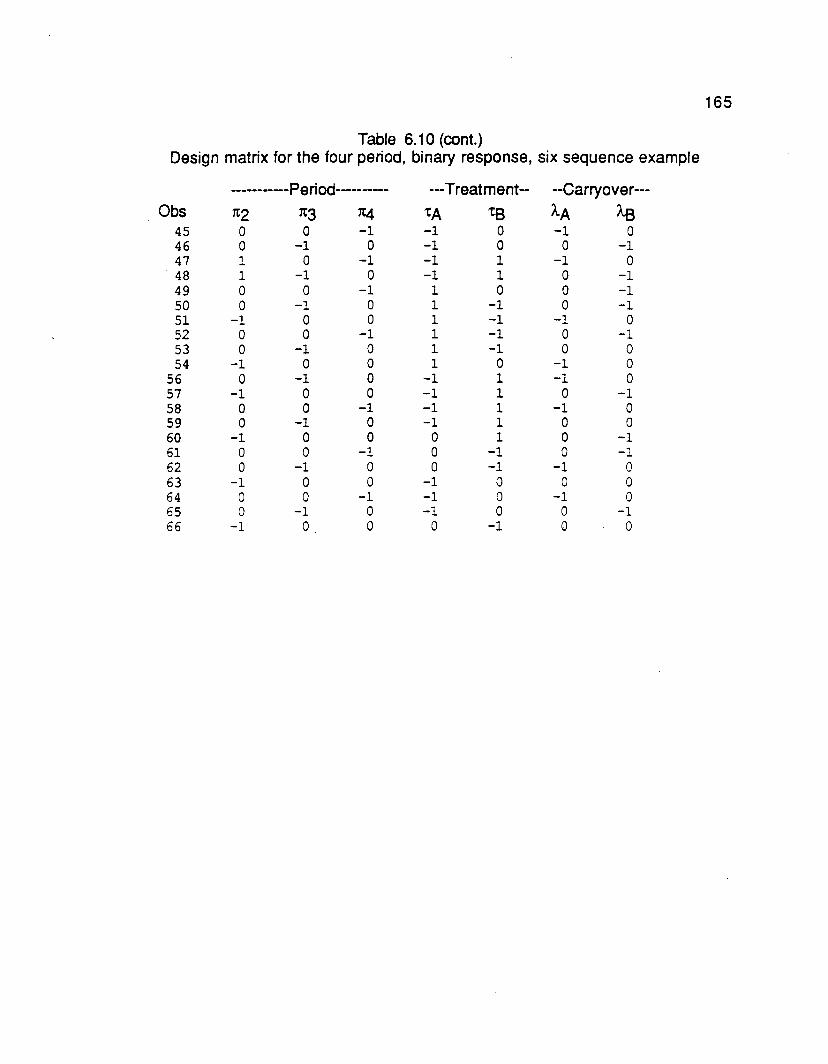
165

Table 6.10 (cant.)Design matrix for the four period, binary response, six sequence example

-----------F'ericxj---------- ---Treatment-- --Carryover---Obs 1t2 1t3 1t4 tA tB AA As

45 0 0 -1 -1 0 -1 046 0 -1 0 -1 0 0 -147 1 0 -1 -1 1 -1 048 1 -1 0 -1 1 0 -149 0 0 -1 1 0 0 -150 0 -1 0 1 -1 0 -151 -1 0 0 1 -1 -1 052 0 0 -1 1 -1 0 -153 0 -1 0 1 -1 0 054 -1 0 0 1 0 -1 0

56 0 -1 0 -1 1 -1 057 -1 0 0 -1 1 0 -158 0 0 -1 -1 1 -1 059 0 -1 0 -1 1 0 060 -1 0 0 0 1 0 -161 0 0 -1 0 -1 0 -162 0 -1 0 0 -1 -1 063 -1 0 0 -1 0 0 064 0 0 -1 -1 0 -1 065 0 -1 0 -1 0 0 -166 -1 0 0 0 -1 0 0

166

Table 6.11

Reduced model estimates - varying multinomial logistic model

Parameter Estimate Std, error P-value

7t2 -0.086 0.261 0.74

7t3 0.538 0.238 0.02

7t4 -0.028 0.199 0.89

tA -1.423 0.202 <0.0001

tB -1.404 0.206 <0.0001

In conclusion these two strategies both agree that a model incorporating just

period and treatment effects is adequate. Notice the high level of agreement

between the parameter estimates in Tables 6.9 and 6,11. Furthermore, there is

period 3 effect, while the effect attributable to periods 2 and 4 relative to the first

period is negligible. Of most important to assess with these results is that

treatments A and B are significantly better than the placebo treatment C. Thenegative sign attached to the estimates for tA and tB reflect the direction that

these treatments tend to produce a decreased severity level (binary

response=O) rather than an increased severity (binary response=1). However,

there is not a discernible difference between treatments A and B.

Computing for this example can be performed with a variety of software

packages. For the two-stage combination method, any categorical program that

provides maximum likelihood estimates for the logistic model is appropriate.

SAS's PROC CATMOD is such a program. For the second step, a weighted

least squares program (GENCAT) was used as it allows for input of a parameter

vector with its associated covariance matrix and provides hypothesis testing.

The second method presented here required a program to be written to

specifically handle the varying length response vectors. This was accomplished

with SAS's matrix language.

167

CHAPTER 7

LOGISTIC MODELS FOR CROSSOVER DESIGNS

FOCUSING ON DISCORDANT SETS OF JOINT OUTCOMES

INCORPORATING A MISSING DATA STRUCTURE

7.1 Introduction

Missing data for any study occurs when a subject's data profile is not complete

for one or more measures. This omission may be due to a design protocol that

did not require information for a particular measure or the incomplete data may

have happened at random. For the crossover design, the presence of missing

data has the potential to be even more prevalent than with other clinical trials.

As the number of periods increases, it is more likely that subjects will miss one

or more of their scheduled visits or drop out of the study. Due to monetary or

management considerations, it may be feasible to randomly select a subset of

patients to participate in only a reduced subset of the periods. Here, the missing

data structure would be a result of design implementation.

None of the existing methods for the crossover design with a categorical

response are applicable to subjects with any missing data. Of all the methods

discussed in the literature review in Chapter 1, including Jones and Kenward's

method, the only recourse is to exclude the entire subject's profile from the

analysis. This loss of information could be substantial in many crossover

studies.

However, the methods discussed in this research do allow for missing data.

The framework established in Chapters 3 through 6 still is applicable and the

product multinomial distribution with varying length response vectors will allow

for the model to include missing data. The three period crossover trial for the

binary response will be presented to illustrate these principles. Furthermore,

missing data could be present in any higher order design for any type of

168

categorical outcome (binary, nominal or ordinal) and the extension seen here

readily applies.

However, it will be necessary to assume that the data is missing by design or

at random. This means that if the data is not intended to be missing but

nonetheless is missing, a underlying random process must have determined

this. This precludes the situation where potential side effects of a particular

treatment cause subjects to drop out of the study while receiving that treatment.

The correlation of a particular treatment with subsequent missing data may not

fall into the category of missing data at random. If the data is missing by design,

it would be necessary that random allocation of subjects to subsets of the

periods have been realized.

7.2 General NotationFor the k-th subject in a crossover design, allow their response Yijk to apply for

the i-th sequence group for the j-th period. Let the indicator variable Oijk=1 if the

k-th subject in the i-th group contributes information for the j-th period.Otherwise this indicator has the value zero. Thus the response profile (Oi1 k,

Yi1 k, Oi2k, Yi2k, . . . . 0iJk, YiJk), represents outcomes for the k-th subject in

the i-th group for the J periods of the trial.

For the simple 2 x 2 trial with a binary response, this implies the following nine

joint responses are possible: (.. ) (which implies that a scheduled subject did

not provide appropriate information for the comparison at hand), (.0) ( a subject

provides information for the second period but not the first), (.1), (0.), (1.),\(00),

(10), (01') and (11). The following section will show how the methods already

presented in this research can be adapted for incomplete data.

7.3 Strategy presented through a three period crossover design

In order to fully consider how missing data impacts the crossover trial,

consider the three period crossover study with a binary response. As an

example, let there be three sequence groups: A:8:C, 8:C:A and C:A:8. The

following four situations can arise: data is provided for all three periods, data is

available for only periods 1 and 2 (possibly indicating a subject who dropped

169

out), data is available for periods 1 and 3, or data is available for only periods 2

and 3. Any of these missing data situations could arise by the mechanisms

discussed in the introduction to this chapter. The situation where data is present

from only one period will not be considered in this analysis. Not only would an

investigator question the use of such information when a multivisit set of

interventions had been planned, but this subject also does not provide any

discriminating information between periods. With no combination of periods to

serve as their own control for treatment comparisons, there is no information as

to preference between any of the periods.

Furthermore, consider that either of the two following assumptions may be

appropriate. Assume that for the period where a patient has missing data, that

subject did not show up for that period and thus received no treatment. Or it may

be the case that the patient did receive treatment in that period and was even

monitored for other variables, but did not provide the crucial outcome

measurement for the analysis under consideration. These two conditions and

the periods to which they apply determine which parameters are estimable. The

following two sections consider each of these cases.

7.3.1 Assuming missing data due to subject not receiving treatment

The subjects will be grouped by the four groupings described above relative

to which periods they provide information. The first group is for those who

completed all three visits, so the extended analysis of Chapter 5, Section 5.2, is

still applicable. Conditioning on the preferences between treatments, the

discordant observations only are considered, thus resulting in the formation of

two conditioned sets. One set being that where only one treatment is preferred

to the other two treatments (Le. (100), (010) and (001) )and the other set being

that where two of the treatments are preferred to a third treatment ( (110), (101)

and (011) ). Refer to Chapter 5 to review how the subject effects are canceled

out differently in each of these conditioned sets. The effects that can beestimated are 1t2, 1t3, 'tA, 'tB, AA and AB, as before. Also, as with the previous

presentations, the parameters are interpreted in terms of the marginal

probabilities and the conditioned sets represent joint conditional probabilities.

170

Consider the subject who did not complete for all three periods. If the patient

did not receive any treatment for the period he has missing data for, then he

only received two of the three treatments. If the subject only has data from

periods 1 and 2, then this reduces to the comparison of the (10) vs (01) for

periods 1 vs 2. This is the focus of Chapters 3 and 4, where the parameters ofinterest are 1t2 effect, treatment effect and the carryover effect of a treatment

from the first period. Refer to Table 4.4 in Chapter 4 where comparison is made

relative to the preference outcomes of (10) vs (01) for an assessment of three

treatments. For the three treatment sequences being considered in this situation

(Le. A:8:C, 8:C:A, C:A:8), the comparison of data from the first two periods

involves the following sequences A:8, 8:C, and C:A. Table 7.1 displays the

numerators of the conditional joint probabilities for each of the missing sets.

When a subject only prOVides information from periods 1 and 3, then

comparisons of the outcomes (10) vs (01) are still of interest. Here the

assumption made for this section comes into consideration. Since the subject is

assumed not to have received any treatment at visit 2, by definition it is not

possible for a carryover effect to exist from period 2 to period 3. Period and

treatment effects are defined in the usual manner. This is reflected in the

parameters displayed in Table 7.1

Similarly, when a SUbject receives only treatments at periods 2 and 3, then

there can be no carryover from period 1 to period 2. However, the carryover

effect from period 2 to period 3 still applies. Refer to Table 7.1.

From these conditional probabilities, the logits are the In of the ratio of the

probabilities where the last probability in the table is the denominator of the

ratio; thus, it is the reference cell. This is consistent with the previous

presentations of this research. Table 7.2 displays these logits and the

associated design matrix. Note that there are a varying number of responses for

the various subpopulations, where subpopulation corresponds to the missing

set by conditioned set by sequence group specification. For the first missing

set, there are four logits per sequence group divided into two conditioned sets;

while for the other missing sets, there is one logit per sequence group.

171

Table 7.1

Numerators of Conditional Joint Probabilities

A:B:C

B:C:A

C:A:B

Missing set:1. all three periods

UQO.lA:B:C exp('tA)

B:C:A exp(1:B)

C:A:B exp(O)

ill.Qlexp(1t2+'tA+'tB+A.A)

exp(1t2+'tB+A.B)

exp(1t2+'tA)

2. periods 1 and 2L1Ql

A:8:C exp('tA)

8:C:A exp('tB)

C:A:B exp(O)


A:B:C exp('tA)

8:C:A exp('tB)

C:A:8 exp(O)


A:8:C exp(1t2+'tB+A.A)

B:C:A exp(1t2+A.B)

C:A:8 exp(1t2)

!Q1!llexp(1t2+'tB+A.A)

exp(1t2+A.B)

exp(1t2+'tA)

LLQll

exp(1t3+'tA+A.B)

exp(1t3+'tA+'tB)

exp(1t3+'tB+A.A)

LQ.1lexp(1t2+'tB+A.A)

exp(1t2+A.B)

exp(1t2+'tA)

LQ.1lexp(1t3)

exp(1t3+'tA)

exp(1t3+'tB)

LQ.1lexp(1t3 +A.B )

exp(1t3+'tA)

exp(1t3+'tB +A.A )

J.Q.Q.Uexp(1t3+A.B)

exp(1t3+'tA)

exp(1t3+'tB+A.A)

!Q.1.ll

exp(1t2+1t3+'tB+A.A+A.B)

exp(1t2+1t3+'tA+A.B)

exp(1t2+1t3+'tA+'tB+A.A)

While the multinomial model is a viable choice to describe this situation, it is

necessary to incorporate the extension proposed in Chapter 6 for a product

Table 7.2

Logits and Design Matrix

172

~ design matrix (X)1st missing set (all three periods) :

151 condjtjoned set :A:8:C (100) vs (001) -1t3 + 'tA - A8 0-1 1 a 0-1

(010) vs (001) 1t2 - 1t3 + 't8 + AA - A8 1 -1 a 1 1 -1

8:C:A (100) vs (001) -1t3 - 'tA + 't8 0-1 -1 1 a a(010) vs (001) 1t2 -1t3 - 'tA + AB 1 -1 -1 a a 1

C:A:8 (100) vs (001) - 1t3 - 't8 - AA 0-1 a -1 -1 a(010) vs (001) 1t2 - 1t3 + 'tA - 'tB - AA 1 -1 1 -1 -1 a

2nd conditioned set ;A:8:C (110) vs (011) -1t3 + 'tA - A8 0-1 1 a 0-1

(101) vs (011),

-1 a 1 -1 -1 a-1t2 + 'tA - t8 - AA

B:C:A (110) vs (011) -1t3 - tA + tB a -1 -1 1 a a(1 01 ) vs (0 11 ) -1t2 + 'tB - A8 -1 a a 1 0-1

C:A:8 (110) vs (011) - 1t3 - tB - AA a -1 a -1 -1 a e(101) vs (011) - 1t2 - 'tA -1 a -1 a a a

2nd missing set (periods 1 and 2):A:B:C (10) vs (01) -1t2 + tA - t8 - AA -1 a 1 -1 -1 aB:C:A (10)vs(01) -1t2 + tB - A8 -1 a a 1 0-1

C:A:8 (10)vs(01) -1t2 - 'tA -1 0-1 a a a3rd missing set (periods 1 and 3):A:8:C (10) vs (01) -1t3 + tA 0-1 1 a a aB:C:A (10) VS (01) - 1t3 - tA + t8 a -1 -1 1 a aC:A:B (10) vs (01) -1t3 - t8 0-1 0-1 a a4th missing set (periods 2 and 3):A:B:C (10)vs(01) 1t2 - 1t3 + t8 - A8 1 -1 a 1 a -1

B:C:A (10) vs (01) 1t2 -1t3 - tA 1 -1 -1 a a aC:A:B (10)vs(01) 1t2 - 1t3 + 'tA - 'tB - AA 1 -1 1 -1 -1 a

multinomial with varying length response probabilities. The design matrix

displayed below allows for this structure.

173

This design matrix has dimension 21 rows by 6 parameters to be estimated. If

the data in a three period crossover design were missing at random, it would be

unlikely that all the combinations of two periods with all sequence groups would

be observed. Deletion of the rows above corresponding to situations that were

unobserved handles this issue. If all combinations do exist (Le. there are 21

rows as above), it could have resulted from a design that was planned to

include incomplete data.

7.3.2 Assuming missing data due to subject receiving treatment but

measurement not recorded

The situation presented here accounts for a slightly different assumption

where the subjects are assumed to have received all of the treatments, but did

not have a recorded value for the outcome of interest. This could have arisen as

a result of a faulty measurement or any other happening that precluded the

patient from having a valid measurement taken for the treatment of that period.

For instance, if the outcome is relief of pain at three hours post treatment, a

patient could have received the treatment but not reported at three hours for the

measurement to be observed.

The modification to this type of assumption corresponding to the missing data

for a period implies that one can consider the carryover effects for the missing

period. Specifically, if a subject in the sequence group A:B:C has missing data

for period 2 then there is still a carryover effect of treatment B from period 2 to be

modeled in period 3. Table 7.3 modifies Table 7.2 to include the additional

carryover effects that can be considered.

Again, modeling is accomplished with a underlying product multinomial

model with varying length response vectors operating on the logits. Similarity of

these six parameters across complete and missing sets can be assessed with a

six degree of freedom test.

Table 7.3

Logits and Design Matrix

~1st missing set (all three periods) ;

174

design matrix (X)

1st conditioned set:A:B:C (100) vs (001) -7[3 + T.A - AB 0-1 1 0 0-1

(010) vs (001) 7[2 - 7[3 + T.B + AA - AB 1 -1 0 1 1 -1

B:C:A (100) vs (001) -7[3 - T.A + T.B o -1 -1 100

(010) vs (001) 7[2 -7[3 - T.A + AB 1 -1 -1 0 0 1

C:A:B (100) VS (001) -7[3 - T.B - AA o -1 0-1 -1 0(010) vs (001) 7[2 - 7[3 + T.A - T.B - AA 1 -1 1 -1 -1 0

2nd conditioned set :A:B:C (110) vs (011) -7[3 + T.A - AB 0-1 1 0 0-1

(101) vs (011) -7[2 + T.A - T.B - AA -1 o 1 -1 -1 0

B:C:A (110) vs (011) -7[3 - T.A + T.S o -1 -1 100

(101)vs(011) -it:2 + 'tB - AS -1 001 0-1 eC:A:S (110)vs(011) -7[3 - ts - AA 0-1 0 -1 -1 0

(101) vs (011) -7[2 - 'tA -1 0 -1 0 0 0

2nd missing set (periods 1 and 2);A:B:C (10) vs (01) -7[2 + T.A - 'tB - AA

B:C:A (10) vs (01) -7[2 + T.B - AB

C:A:B (10) vs (01) -7[2 - 'tA

3ed missing set (periods 1 and 3):A:B:C (10) vs (01) -7[3 + 'tA - AS

B:C:A (10) vs (01) -7[3 - 'tA + T.B

C:A:B (10) vs (01) -7[3 - 'tS - AA

4th missing set (periods 2 and 3):A:B:C (10) vs (01) 7[2 - 7[3 + 'tS + AA - AS

B:C:A (10) vs (01) 7[2 -7[3 - 'tA + AB

C:A:B (10) vs (01) 7[2 - 7[3 + 'tA - T.B - AA

-1 0 1 -1 -1 0

-1 0 0 1 0-1

-1 0 -1 0 0 0

0-1 1 00-1

0-1 -1 1 0 0

0-1 0 -1 -1 0

1 -1 0 1 1-1

1 -1 -1 0 0 1

1 -1 1 -1 -1 0

175

7.4 Period Association Parameters

As consistent with the theme of the other chapters, it is important to consider

what happens when this model does not provide adequate goodness of fit.

When the assumption of conditional independent period responses is not valid,

then incorporation of additional parameters to explore lack of fit can be used.

Since lack of fit implies deviation from the conditional independence

assumption, these effects in some sense capture that dependency structure.

The design matrix of Table 7.3 has dimension 21 x 6, thus there are an

additional 15 degrees of freedom to account for relative to this design.

Referring back to section 5.3.1, the (J and ~ parameters are defined and

interpreted for the complete three period design. These contrasts will still apply.

The notation here needs to be modified slightly for the conditional jointprobability from 1ti to 1tim where m=1, 2, 3, 4 corresponding respectively to the

missing set profiles. The m=1 refers to the complete design and m=2, 3, 4

corresponds to the partial two period designs, respectively as displayed in

Table 7.3. For each of the i-th sequences, the following relationships exist:

In (1ti1 (100) / 1ti1 (001) ) = In (1ti1 (110) / 1ti1 (011) )

= In (1ti3(1 0) / 1ti3(01 ) ).

The equivalent contrast across the i-th sequence is

(1 a -1 a a a a1 a a a a -1 0).

The parameters (J1, 1 and (J1 ,2 of Table 7.4 are associated with these.

With the complete three period design, the following equivalence was noted:

In (1tj 1(11 0) / 1ti1(0 11)) - In (1ti1(101 ) / 1ti1(011 ) ) = In (1ti1(010) / 1tj1(001) ).

In the partial designs, there is a similar relationship

In (1ti3(1 0) / 1ti;3(01)) - In (1ti2(1 0) / 1ti2(01) ) = In (1ti4(1 0) / 1ti4(01) ).

Furthermore, another relationshup across the complete to the partial designs

exists:

In (1ti1(010) /1ti1(001)) + In (1ti1(101)/1ti1(011)) = In (1ti3(10)/1ti3(01))

This corresponds to the three degree of freedom contrast for each sequence

denoted by (J2,1 , (J2,2 and (J2,3:

(0 -1 1 -1 0 0 aa a 0 0 -1 1-1

176

0-1 0 -1 0 1 0).

When the model of Table 7.3 does not provide a good fit, then theseequivalences do not hold. So additional parameters, denoted as 0' association

parameters are needed to explain further relationships. Table 7.4 displays what

these five 0' parameters are where the first two correspond to the first type of

equivalence and the last three relate to other equivalence. The 0'1,1 and 0'2,1

corresponds to the complete designs only. The 0'1,2 and 0'2,3 mixes the

equivalence across the studies (complete and partial). The 0'2,2 relates only to

the partial study.

Augmenting these five columns sidewise to the!- of Table 5.3 provides an 11

degree of freedom test. Since:c. has 21 rows, there are 10 additional degrees of

freedom. When each of t~e ers are allowed to vary across the sequences, there

are two association by sequence group (t}'s) interactions to consider. Thus, the

five O"s imply 10 t}'s.

As an additional note of interest, it is possible to have a study with only the

partial designs included (m=2, 3 and 4). When the complete three period design

is not included for a three period crossover, it is still possible to estimate all six

parameters (21t's, 2't's, 2A.'s). The additional three degrees of freedom

correspond to 0'2,2 and their two associated t}'s.

7.5 Extension to higher order designs and to nominal and ordinal outcomes

When the response is nominal or ordinal rather than binary, the same

principle of dividing the groups by the specific periods observed is still

appropriate. The number of parameters increases to reflect the categoricaloutcome. For instance, with a nominal response with A categories, 1t2 is

extended to the parameters 1t21, 1t22, .....1t2,A-1. Aefer to other chapters to

see how the nominal model can be reduced when the response is ordinal.

Furthermore, when higher order designs are used, division of the subjects into

missing sets still allows for all of the available data to be used. The same logic

is applied which allows for the responses to be partitioned into the conditioned

sets. For instance, in a four period design with a binary response, when all

177

Table 7.4

Additional Assocation parameters

~ ~1J. SI12~SI~~U1st missing set (all three periods) :

1st conditioned set:A:B:C (100) vs (001) -1t3 + 'tA - AB 1 1 0 0 0

(010) vs (001) 1t2 - 1t3 + 'tB + AA - AB 0 0 -1 0 -1

B:C:A (100) vs (001) -1t3 - 'tA + 'tB 1 1 0 0 0

(010) vs (001) 1t2 -1t3 - 'tA + AB 0 0 -1 0 -1

C:A:B (100) vs (001) -1t3 - 'tB - AA 1 1 0 0 0(010) vs (001) 1t2 - 1t3 + 'tA - 'tB - AA 0 0 -1 0 -1

2nd conditioned set:A:B:C (110) vs (011) -1t3 + 'tA - AB -1 0 1 0 0

(101)vs(011) -1t2 + 'tA - tB - AA 0 0 -1 0 -1

B:C:A (110)vs(011) -1t3 - 'tA + 'tB -1 0 1 0 0

(101)vs(011) - 1t2 + 'tB - AB 0 0 -1 0 -1

C:A:B (110)vs(011) -1t3 - tB - AA -1 0 1 0 0(101) vs (011) - 1t2 - 'tA 0 0 -1 0 -1

2nd missing set (periods 1 and 2):A:B:C (10)vs(01) -1t2 + 'tA - 'tB - AA 0 0 0 -1 o ~

B:C:A (10)vs(01) - 1t2 + 'tB - AB 0 0 0 -1 0

C:A:B (10) vs (01) - 1t2 - 'tA 0 0 0 -1 03rd missing set (periods 1 and 3):A:B:C (10)vs(01) -1t3 + 'tA - AB 0 -1 0 1 1

B:C:A (10)vs(01) -1t3 - 'tA + 'tB 0 -1 0 1 1

C:A:B (10)vs(01) - 1t3 - 'tB - AA 0 -1 0 1 14th missing set (periods 2 and 3):A:B:C (10)vs(01) 1t2 - 1t3 + 'tB + AA - AB 0 0 0 -1 0

B:C:A (10)vs(01) 1t2 -1t3 - 'tA + AB 0 0 0 -1 0

C:A:B (10) vs (01) 1t2 - 1t3 + 'tA - 'tB - AA 0 0 0 -1 0

178

subjects are observed there are three conditioned sets with 3, 5 and 3 logits

respectively per sequence group. For those subjects who only provided three of

the four responses, two conditioned sets apply with two logits for each per

sequence group. Similarly for the subset of patients who only had information

for two of the periods, a comparison of (10) vs (01) for those two periods is

applicable resulting in one logit per sequence group. All of these subsets can

be combined into one comprehensive model to estimate the period, treatment

and carryover effects.

7,6 Example

The example of this chapter is the data from Koch, Imrey and Reinfurt (1972),

It is example 2.4 of their paper which represents modified hypothetical data from

the UNC Highway Safety Research Center. It represents the pass / fail status of

drivers subject to three different cars across three examining periods. Because

of time scheduling problems or cost considerations, some of the drivers did not

attend all examinations. This incomplete data structure provides an excellent

example of a three period crossover design with missing data. The three

periods correspond to the three times of test administration. The treatments ar.e

the car selection and examining procedure and will be changed to be A, 8 and

C to be consistent with the notation of this research. In addition to the group of

drivers completing all three periods, there are those whose partial data

encompasses periods 1 and 2 and those with just periods 1 and 3. Table 7,5

displays the data counts for this structure.

The main effects design matrix of section 7,3,1 is fit assuming that the

missing data occurred where the subject did not receive the test procedure.

Table 7.6 summarizes the data of this model which does not provide a good fit(QL = 27.71, df=12, p-value=0.01). While the period 2 effect is borderline

179

Table 7.5

Counts of drivers for complete and partial studiesMissing set:1. all three periods

llillll !Q1.Ql LQ.Q.1lA:B:C 5 9 248:C:A 16 22 3C:A:B 10 6 14

w.w. llilll LO.1.llA:B:C 10 13 158:C:A 13 13 9C:A:B 13 25 6

2. periods 1 and 2illll LO.1l

A:B:C 8 21B:C:A 10 8C:A:B 11 6

3. periods 1 and 3illll iQ.1l

A:B:C 7 10B:C:A 8 11C:A:B 18 5

significant, there is no significant period 3 effect. Both treatment effects are

significant while there does not appear to be significant carryover.

Due to this lack of fit, it is relevant to consider what association parameters

may contribute to explain the lack of fit. From Table 7.4, it should be noted thatthe association parameter <J2,3 is not estimable because there is not a partial

set corresponding to just periods 2 and 3. Table 7.7 summarizes the results of

such a model incorporating period, treatment, carryover effects as well as fourassociation parameters. The fit of this model is still not adequate (QL=23.65,

df=8, p-value=0.003) and the association parameters do not seem to fullycapture this lack of fit. the fact that <J1 ,1 approaches significance suggests some

variation attributable within the condition set for the complete study.

An obvious way to further define this lack of fit is to model period and

treatment parameters separately for each of the three studies (Le. the complete,

180

partial with 1 and 2, and partial with 1 and 3). Note that the nonsignificance of

carryover effect in Table 7.6 and 7.7 justifies it not be included in this model.

The design matrix of Table 7.8 accomplishes this. The goodness of fit of thismodel is improved but still not satisfactory with QL=17.11, df=8, p-value=O.03.

Hypothesis tests relative to the parameter vector ~ = (1t2,1, 1t3,1 ' 'tA,1 ' 'tB,1 ' 1t2,2,

'tA,2, 'tB,2, 1t3,3, 'tA,3, 'tB,3) reveal that the two period 2 effects are equivalent

(Qc=0.71, df=1, p-value=0.40) and the two period 3 effects are equivalent

(Qc=0.63, df=1, p-value=0.43). Similarly, the three treatment A effects for the

three studies are equivalent (Qc=O.94, df=2, p-value=0.62). However, not all of

the treatment B effects are equivalent (Qc=5.83, df=2, p-value=0.05). A reduced

design matrix can thus be considered which allows for common period 2, period

3 and treatment A effects while allowing the treatment B effect to vary for each of

the studies.This design has an adequate goodness of fit QL= 19.27 , df=12 , p-

value=0.08. The parameter estimates are shown in Table 7.9. While there are

no significant period effects. there is a strong treatment A effect. Also. there are

significant treatment effects for the complete study and the partial set with just

periods 1 and 3. However, the treatment B effect for the partial set with periods 1

and 2 is not significant. This presents a dilemna in explaining why the treatment

B would perform differently relative to the missing data structure.

7.7 Discussion

The methods of a logistic model applied to the conditional joint probabilities

can be applied to estimate parameters defined from marginal probabilities and

to allow for incomplete data. The same parameter definitions, model

specification and structural implementations can be used as those presented in

the previous 4 chapters. Furthermore, an assessment can be made when the

model assumptions do not provide an adequate fit.

Table 7.6

Main effects model

181

Parameter

1t2

1t3

'tA

tsAAAS

Estimate-0.37

-0.15

-0.70

-0.44

0.45

0.24

~

0.22

0.18

0.21

0.22

0.33

0.31

p-value0.09

0.40

0.001

0.05

0.17

0.44

Table 7.7Main effects model with association parameter

Parameter

1t2

1t3

tA'tS

AAAS(11,1

(11,2

(12,1

(12,2

Estimate-0.45

-0.07

-0.75 ~

-0.43

0.31

0.24

-0.47

0.27

-0.19

0.39

~

0.24

0.20

0.23

0.23

0.33

0.38

0.24

0.31

0.14

0.27

p-value0.06

0.75

0.001

0.06

0.17

0.42

0.06

0.39

0.17

0.14

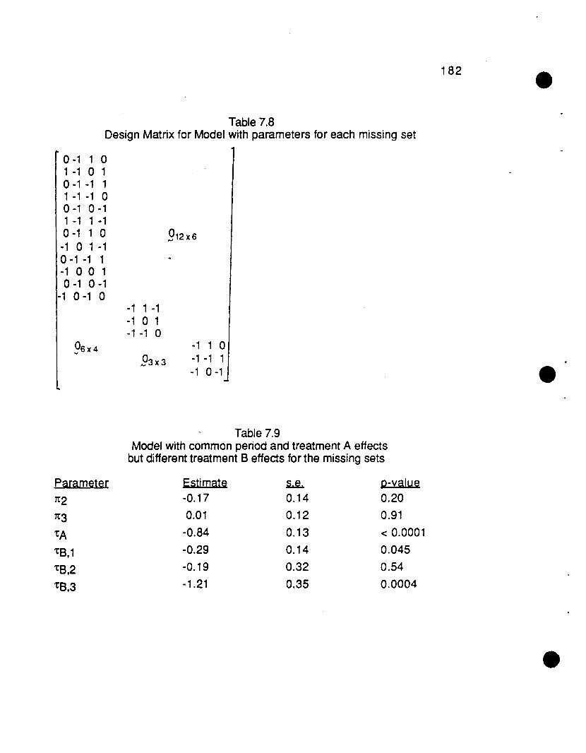
Table 7.8Design Matrix for Model with parameters for each missing set

0-1 1 01 -1 0 10-1-1 11 -1 -1 00-1 0-11 -1 1-10-1 1 0 912 x6

-1 0 1 -10-1 -1 1-1 0 0 10-1 0-1

-1 0 -1 0-1 1-1-1 0 1-1 -1 0

182

.96x4 -1 1 0-1 -1 1-1 0-1

Table 7.9Model with common period and treatment A effects

but different treatment B effects for the missing sets

Parameter Estimate ~ p-value

1t2 -0.17 0.14 0.20

1t3 0.01 0.12 0.91

tA -0.84 0.13 < 0.0001

'tB,1 -0.29 0.14 0.045

'tB,2 -0.19 0.32 0.54

tB,3 -1.21 0.35 0.0004

183

CHAPTER 8

REVIEW OF THE METHOD OF

JONES AND KENWARD

8.1 Introduction

Byron Jones and Michael G. Kenward from the University of Kent at

Canterbury, UK have recently developed a model for analyzing categorical data

from crossover designs. They have published a text book Design and Analysis

of Cross-over Trials (1989) which provides in Chapter 1 a presentation of the

history of crossover designs. Chapter 2 focuses on the 2 x 2 trial for a

continuous measure. Of interest here is that Chapter 3 deals with crossover

trials with a categorical outcome. The other chapters deal further with the

continuous outcome. As a precursor to their chapter on the categorical

response, they have published two other relevant articles: "Modeling Binary and

Categorical Cross-over Data" (1988 ASA Proceedings) and "Modeling Binary

Data form a Three Period Cross-over Trial" (1987 Statistics in Medicine, Vol. 6 ).

Their basic approach focuses on the joint response probabilities and

incorporates a log-linear model. As with the proposed strategy, it falls into the

general class of log-linear models and operates on the logits. Likelihood ratio

statistics can be used to judge the significance of effects that are defined

relative to the joint probabilities. The modeling of p dependent binary or

categorical random variables in accomplished with a generalization of a logistic

regression model. They also provide a strategy for calculating exact conditional

probabilities. For the 2 x 2 trial, this method involves enumerating all 2 x 4

tables for the two sequence groups by their four joint binary outcomes. This

computation becomes prohibitively difficult as the size of the tables increases.

Kenward and Jones allow for the extension to responses with more than 2

outcomes and to higher order designs. The effects that are modeled are period,

treatment, carryover, dependency (reflecting the correlation across the period)

184

and dependency by group interaction (aI/owing this dependency to vary across

the sequence groups.). The subject effects are assumed to be random, and so a

combination of intra- and inter-subject analysis results. In this regard, the role of

subject effects is incorporated through the dependency and dependency by

group factors.

8.2 General Notation and Model Structure

The general notation used by Kenward and Jones is similar to that of the

proposed methods in this research. This will aid in a comparison of the two

methods. The response Yij applies to a subject's response in the i-th sequence

group at the j-th period. They assume random subject effects. For the g groups

and the P periods, the general model has the form

log [ Pr (Yi1 =Yi1, .... Yip=Yip)] =

~ +! Yj" (Yj' ) +f fa ... (Yj' , Y i" ), 1 J J , 1 ',' 1 II J J~ J- J-~

(8.2.1 )

Assuming an underlying product multinomial distribution, the logits of each of

the joint outcomes with respect to the last outcome are the functions on which

the m.odel is based and effects are interpreted. Since modeling is based on thelog odds ratio or logits, the Ili which are normalizing constants, are viewed as,nuisance terms. They allow the expressions for the joint outcomes to beprobabilities that sum to unity. Thus exp(lli) represents the denominator term.

The parameter Yij corresponds to effects occurring in the i-th group at the j-th

period. These encompass period effect (1t), treatment effect ('t) and carryover

effects (A). The all' represent the dependency between periods j and j' for the

same subject for the joint outcome of the two events. Note that the effects 1t, 't, A,a and ~, while notational/yare like those proposed in the other chapters, are

defined on the joint rather than the marginal probabilities.

For instance, for the first sequence group at the first period, with a response

value of zero :

Y11 (0) = 1l(0) + 1t1 (0) + 't1 (0)

185

where Jl(O) is the mean or normalizing parameter. Jones and Kenward note

simplifications necessary in their model to account for redundancy. For the J

period effects, only J-1 parameters are needed. Specifically, one need only tomodel1t instead of both 1t1 and 1t2 for a two period design. The same is true for

all of the other parameters. This model has the general matrix notation ~=~~

where L is the logs of the joint probabilities and ~ are the expanded yand cr- -parameters. The design matrix X relates the two.

~

For the binary outcome, Jones and Kenward outline a general strategy to

arrive at their model. Assuming a general log-linear model for each period, they

multiply these probabilities to arrive at joint probabilities under the assumption

of independence. Then to account for the lack of independence, they argue thatthe cr and ~ association parameters capture the difference due to the

dependency or correlation that exists. The random subject effects are not

explicitly specified but incorporated into this association structure.

Jones and Kenward fit the log-linear model to the observed joint counts

assuming Poisson errors. This is equivalent computationally to assuming an

underlying product multinomial distribution. Framing this problem in terms of

Poisson sampling allows their computing needs to take precedence in theformulation of the model. Specifically, this introduces extraneous parameters Jl

and a (to be described further in the following sections.). This is different from a

model specification that relies on the intuitive multinomial sampling. For the

methods of this research, which also rely on the multinomial specification, when

parameters were introduced, they had an obvious interpretation relative to the

effects of the crossover design. This is particularly true with the association

parameters. The Jones and Kenward model can be computed with procedures

assuming an underlying multinomial; however, to be consistent with their

notation, the following presentation will assume a Poisson sampling.

8.3 Two Period Trial with Binary Response

The 2 x 2 classical design provides the simplest framework within which to

begin to understand this design. The general from of the model reduces to

In [ Pr (Yi1 =yi1, Yi2=yi2)] = Jli + 'Yi1 (Yi1) + YJ2(Yi2) + cr12(Yi1, Yi2)

(8.3.1 )

186

where Yi1 and Yi2 = 0 or 1 according to the binary response. The model in Table

8.1 is the Jones and Kenward model for the two period design.

Table 8.1

Ln of the Joint Probabilities

Outcome SeQuence GroupAjl ~

(00) J.L 1+ (J + ~ J.L2 + (J - ~

(01) J.L 1 + a + 1t + 't - A. - (J - ~ J.L2 + a + 1t - 't + A. ~ (J + ~

(10) J.Ll +a-1t-'t-(J-~ J.L2+a-1t+'t-(J+~

(11) J.Ll+2a-A.+(J+~ J.L2+2a+A.+(J-~

The parameters are defined relative to the joint probabilities and are as follows:J.L1 =normalizing constant for the first sequence group

J.L2 =normalizing constant for the second sequence group

a =probability of success

1t = period effect

't =treatment effect

A. =carryover effect

(J = dependency parameter, association across the periods

~ = groups by dependency interaction, association that varies

across the sequence groups

(8.3.2)As a note of clarification, the a here refers to a reference probability. This is not

to be confused with the a of the previous chapters which represent subject

effects. The other 1t, 't and A. parameters have similar meanings to those in

previous chapters, although defined from a different basis. If one were using a

computing program with a Poisson framework, the following full design matrix

would apply, where the first four rows correspond to the first sequence group

and the last four rows for the second group. The responses are listed in the

order as presented in Table 8.1

187

100000111 0 1 1 1 -1 -1 -11 0 1 -1 -1 0 -1 -11 0 2' 0 0 -1 1 1o 1 0 0 0 0 1 -1o 1 1 1 -1 1 -1 1o 1 1 -1 1 0 -1 1o 1 2 0 0 1 1-1

Taking their model and expressing it in terms necessary to program with an

underlying multinomial distribution, then the following Table 8.2 applies. The

cell of (00) will be used as the reference cell from which to compute logits. This

choice vs that of the (11) cell is arbitrary.

SequenceA:8

B:A

Logits(11) vs (00)

(10) vs (00)

(01) vs (00)(11) vs (00)(10)vs(00)(01) vs (00)

Table 8.2Parameter expression2a- Aa - 1t - 't - 20' - 2t}a + 1t + 't - A - 20' - 2t}

2a+Aa - 1t + 't - 20' + 2t}a + 1t - 't + A - 20' + 2t}

Design Matrix2 0 0 -1 0 0

1-1-10-2-21 1 1 -1 -2 -2200 1 0 01 -1 1 0 -2 21 1 -1 1 -2 2

For the two sequence groups, the log odds ratio ( In[ (00) (11) I (01) (10) ] ) is

40' + 411 for A:8 and 40' - 411 for 8:A. Thus, the II parameters capture the

departure from homogeneous odds ratios across the sequence groups.

The interpretation of the parameters and analysis is through the joint

probabilities. Given this framework, the marginal probabilities have a

complicated expression as seen in equation 8.3.3. Assume that the A and II

association parameters are essentially zero so as not to be included in the

model. The first order marginal for period 1 is the probability that the first period

has a positive response summed across the responses of the second period.

For the sequence group A:8Pr (Yi1 =1) = [exp(2a) + exp(a - 1t - 't - 20') ] I

[1 + exp(2a) + exp(a -1t - 't-2O') + exp(a + 1t + 't - 20')]

Pr (Yi2 =1) = [exp(2a) + exp(a+1t+'t -20') ] I

[ 1 + exp(2a ) + exp(a - 1t ~ 't -20') + exp(a + 1t + 't - 20') ]

188

(8.3.3)

The period, treatment and carryover effect cannot be interpreted from the

expression for the marginal probabilities. These can be compared to the

marginal probabilities of equation 3.3.1 for the 2 x 2 design. Note that even if

period effects are not included, the joint probabilities do not have a simple

marginal probability representation.

The example that Jones and Kenward present in their papers and text book

for the classical 2 x 2 trial is a study of heart data comparing an active treatment

A vs a placebo B. Thirty four subjects received the treatments in the order A:B,

while 33 were assigned to the B:A sequence. The outcomes are 0 for normal

heart response on an electrocardiogram reading and 1 for abnormal response.

Either of the previous models produces test statistics equivalent to that

presented by Jones and Kenward.

Table 8.3Heart Data for a 2 x 2 trial

SeQuenceA:BB:A

Ull llQl6 09 4

J.Q.1l62

LQQl2218

Fitting the full model, Jones and Kenward note the following results in their

ASA Proceedings paper (1988). The first parameter they test is the t} parameter

which is the sequence group by association interaction. With a X2=1.44 (1 df),

this is nonsignificant at a=0.05. Thus the dependency structure is the same for

the two groups, implying homogeneous odds ratios. Furthermore, the A.

carryover parameter is nonsignificant with X2=1.33 (1 df). The treatment effect

of the active treatment is significant at a=0.05 (X2=5.85, 1 df). The estimate of

this effect is 1.63 (s.e.=0.78). Thus, a reduced model involves 1t, t and cr

parameters, and the estimated OR Kenward and Jones present is exp(1.63) =5.1.

In their text book, they present the same example, still proceeding to test that t}

and A. are nonsignificant in the presence of the fully specified model. Here the

estimates they produce are ~ = (a, 1t, t, cr) with ~ = (-0.490, 0.365, 0.814, 0.883).N 'V

(From their two presentations they change the binary outcome of 0/1 reflecting

189

normal/abnormal to abnormal/normaJ. The former notation will be used to

maintain consistency and comparability). Also, note that their estimate of the

treatment effect changes (one being twice the value of the other). This

discrepancy could be due to a coding difference, the former result could bave

resulted from reference cell coding and the latter due to cell mean effect coding.

Assuming that their text book presentation corrected any typographical errors or

oversights, the later 't will be used. Thus, the OR Kenward and Jones reported

should be exp(2't) = exp(2 * 0.814) = 1.5 which agrees across the two

descriptions.

One crucial issue that Kenward and Jones overlook is that the presence of thezero count in this table prevents the estimation of the full parameters vector (Jl1 ,

Jl2, a, 1t, 't, A, cr, t}) in the Poisson case or ( ex, 1t, 't, A, cr, t}) in the multinomial

case. Their test of t} in the presence of the other parameters is troublesome in

that there are not enough available degrees of freedom to provide an estimate

or a test.Implementing their reduced model of a, 1t, 't and cr, the estimates they display

have been verified with either computing framework. Of these parameters, the

treatment and association parameters are significant.

For comparison to the Kenward and Jones X2 = 5.85 for the hypothesis of no

treatment difference, consider the Gart strategy. To apply this to the 2 x 2 table

of discordant responses, yields a chi-square statistic of 5.5 (adding the value of

0.5 to all cells to adjust for the zero cell count). These test statistics are also

similar to the standard X2 score statistic which has the value of 6.0.

A confidence interval for the odds ratio exp(2't) is shown below for the Gart

estimate of 't=0.79 (s.e.=0.42). Note how close this estimate is to Jones and

Kenward estimate of 0.814. Referring to equation 3.3.3, the 95 % confidence

interval for In OR is (-1.69, 4.85).

8.4 TWO period Trial with Ordinal Response

When the two period crossover design involves an ordinal or nominalcategorical response, the model of Section 8.2 still applies. The outcomes Yi1

and Yi2 = 1, 2, . . . r apply to r response levels. Jones and Kenwrd do not

explicitly specify their model in terms of parameters for the nominal or ordinal

190

outcome. but instead choose to characterize the effects of this model through a

grouping representation in a computing specification. For instance, they display

the two sequence groups with values 1 and 2 respectively depicting a dummy

variable representation. Problems with this characterization that relate to

inconsistencies with the appropriate model and associated degrees of freedom

will be considered.

Displayed in Table 8.4 are the types of parameters implied by Kenward and

Jones computing procedure for nominal data. The parameters of Table 8.4 were

arrived at with the same general strategy that Kenward and Jones used for the

binary, two period case. The entries of this table correspond to the natural

logarithm of the joint probabilities. Note that for convenience of presentation, the

table has been divided into two sections but actually each sequence by joint

outcome is the sum of all 18 parameters. Specifically, for sequence A:8Pr(Y11 =1, Y12=1) = exp(l·ll + al + a2 + a3 + a4 + ~l +~ + ~3 + ~4 )

The 18 parameters are defined as follows :J.11 = normalizing constant for the first sequence

J.12 = normalizing constant for the second sequence

(12 = probability of observing the response category 2

(13 = probability of observing the response category 3

1t2 = 2nd period effect for the response category 2

1t3 = 2nd period effect for the response category 3

t2 = treatment 8 effect for the response category 2

t3 = treatment 8 effect for the response category 3

A,2 = carryover effect for treatment 8 for the response category 2

A,3 = carryover effect for treatment 8 for the response category 3

a1 = association parameter -(in terms of odds ratio (33)(11) / (31) (13) )



a4 = association parameter-

(in terms of odds ratio (32)(11) / (31) (12) )

SeQuence Joint OutcomeA:8 (11)

(12)

(13)

(21 )

(22)

(23)

(31 )

(32)

(33)

8:A (11)

(12)

(13)

(21 )

(22)

(23)

(31 )

(32)

(33)

Table 8.4

Ln of Joint Probabilities

Ln(Joint Probs,)

111III + <XZ + 1tZ + tz

III + <X3 + 1t3 + t3

III + <xz

III + Z<XZ + 1tZ + tz

III + <xz + <X3 + 1t3 + t3

III + <X3

III + <xz + <X3 + 1tZ + tz

III + Z<X3 + 1t3 + t3

112IlZ + <XZ + 1tZ + A2

112 + <X3 + 1t3 + A3

IlZ + <XZ + t2

IlZ + 2<XZ + 1tZ + tz + AZ

IlZ + <XZ + <X3 + 1t3 + t2 + A3

IlZ + <X3+ t3

IlZ + <XZ + <X3 + 1t2 + t3 + AZ

112 + Z<X3 + 1t3 + t3 + A3

191

A:8 (11 )

(12)

(13)

(21 )

(22)

(23)

(31 )

(32)

(33)

0'1 + O'Z + 0'3 + 0'4 + ~l + ~Z + ~3 + ~4

- 0'3- 0'4 - ~3 - ~4

--01 - O'z - ~l - ~2

- O'z - 0'3 - ~ - ~3

0'3 + ~3

O'Z +~

--01 -0'4-~1 -~4

0'4 + ~4

0'1 + ~l

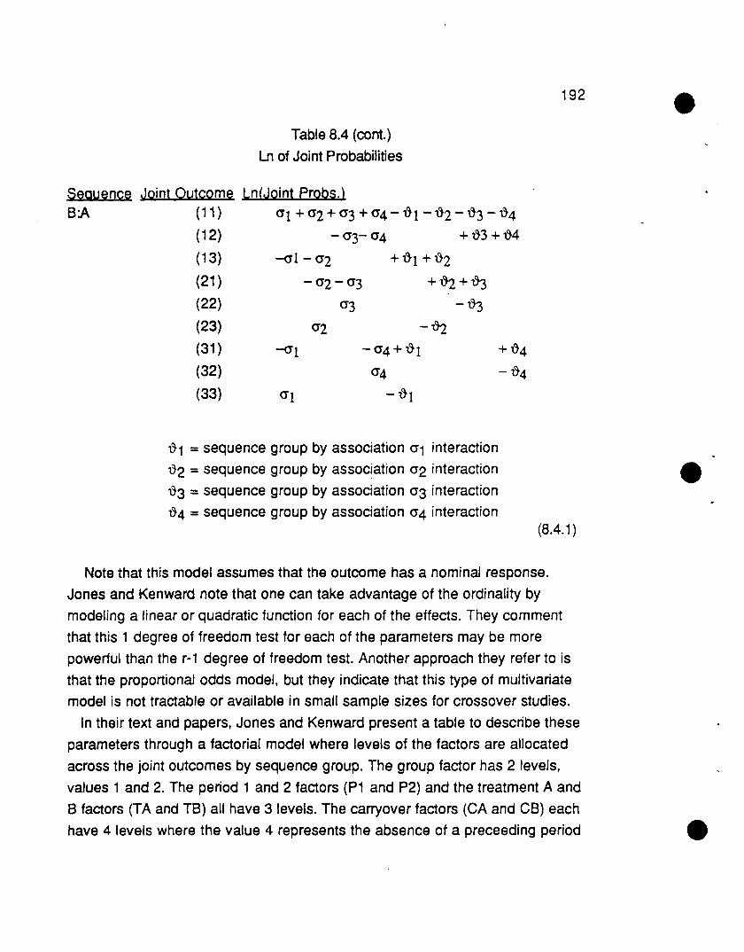
192

Table 8.4 (cont.)

Ln of Joint Probabilities

SeQuence6:A

Joint Outcome(11 )

(12)

(13)

(21)

(22)

(23)

(31 )

(32)

(33)

Ln(Joint Probs.)

<Jl +<J2+<J3+<J4-~1-~2-~3-~4

- <J3- <J4 + ~3 + ~4

-<11 - <J2 + ~1 + ~2

- <J2 - <J3 +~ + ~3

<J3 - ~3

<J2 -~

-<11 -<J4+~1 +~4

<J4 - ~4

<Jl - ~1

~1 =sequence group by association <J1 interaction

tt2 = sequence group by association <J2 interaction

tt3 = sequence group by association <J3 interaction

tt4 = sequence group by association <J4 interaction(8.4.1 )

Note that this model assumes that the outcome has a nominal response.

Jones and Kenward note that one can take advantage of the ordinality by

modeling a linear or quadratic function for each of the effects. They comment

that this 1 degree of freedom test for each of the parameters may be more

powerful than the r-1 degree of freedom test. Another approach they refer to is

that the proportional odds model, but they indicate that this type of multivariate

model is not tractable or available in small sample sizes for crossover studies.

In their text and papers, Jones and Kenward present a table to describe these

parameters through a factorial model where levels of the factors are allocated

across the joint outcomes by sequence group. The group factor has 2 levels,

values 1 and 2. The period 1 and 2 factors (P1 and P2) and the treatment A and

8 factors (TA and T6) all have 3 levels. The carryover factors (CA and CB) each

have 4 levels where the value 4 represents the absence of a preceeding period

193

1 effect. This structure is somewhat inconsistent with the theoretical model they

proposed because the degrees of freedom for the factors do not match to the

appropriate degrees of freedom required by the effects. Furthermore,

singularities or redundancies are evident among a full speification. When the

coding scheme for these factors is implemented, a model (from the multinomialframework) with parameters 2a's, 2x's, 2t's, 21's and 4 cr's should consist of 12

df leaving a 4 df test for goodness of fit. However, with their coding factors, the

model with a residual 4 df test encompasses 13 df attached to the factors and so

there will be redundancy among some of the parameters expressed this way.

The two period example. for the condition of primary dysmenorrhea that Jones

and Kenward describe in both their text book and their paper in the ASA

proceedings involves a response with three levels. Two treatments are

administered where A is a placebo and B is an active high dose analgesic.

Relief is measured on a three point scale: 1= none or minimal, 2= moderate

and 3= complete relief. Sixteen patients received the treatments in the order

A:B, while 14 received treatments in the reverse order. Notice in the following

Table 8.5, the data contains a large number of zero counts for this ·moderately

small sample size. Specifically, observe that both responses (32) and (33) are

unobserved in both of the sequences.

Sequence

A:B

B:A

(11 ) (12)

2 33 2

Table 8.5Primary Dysmenorrhea Data

(13) (21) (22) (23) (31) (32) (33)

6122000

011 1600

IQ1aJ.16

14

Jones and Kenward proceed to fit a model with 12 parameters (the 2a's, 2 x's, 2

t'S, 2 A's, 4 a's) and report a 4 degree of freedom test for the ~ parameters. As

just comented on with their factor specification, they actually have a model with

13 df with aliased components. They comment in their test that they actually

used another computing approach to remedy aliased effects. However, thepattem of the zero cells in the data prevents an explicit test of the ~'s. Looking at

the structure of the zero cells implies that only a2 and a3 (out of the 4 a's) can

194

be estimated. Neither CJ1 or CJ4 can be estimated. Similarly t}3 is the only t}

parameter that can be estimated. This is true regardless of whether one

estimates the parameters and statistics via a multinomial or Poisson framework.

There exist estimability dilemnas with computation if the zero cells are left as

zero cells. Jones and Kenward apparently replace the zero count with a very

small value and then proceed.

In a subsequent model, Jones and Kenward further determine that thecarryover effects, as well as the four t}'s are nonsignificant. Thus they fit a model

with 2 a's, 2 1t'S, 2 t's and 4 a's. In their text book and their ASA Proceedingspaper, they report their estimate for the crucial treatment parameters as t2 =

0.748(+0.768) and t3=2.89(+1.11), where the 2 df likelihood ratio statistic is

significant X2= 13.97 (=17.23 - 3.27). This computing was done with the

program GUM via assuming Poisson sampling errors. None of these values

could be verified from either a Poisson or multinomial computing framework.

With the appropriate multinomial framework and accounting for the zero data

counts through deletion of the (32) and (33) outomes and thereby use of only 2a's with 2 1t'S, 2 t'S and 2a's, the values for the effect should be t2 = 1.58

(s.e.=0.99), t3 = 3.72 (s.e.=1.47) where the likelihood ratio statistic is 10.02

(17.58 - 7.56,df=2) for elimination of t'S.

Jones and Kenward do not handle their zero counts this way. They choose to

replace the zeros with the value 0.00000001. However, such a small value still

results in problems of near singularities. To further consider this issue, 5

different ways of handling zero data were implemented and compared. The first

is probably the most satisfactory, where zero counts are left as zero counts. The

outcomes (32) and (33) are omitted from analysis leaVing 12 total available

degrees of freedom for a Poisson model analysis. The second strategy uses the

Kenward and Jones model where zero counts are replaced with the value

0.00000001. Note that these numbers, displayed in Table 8.6, will not match

what Kenward and Jones display because of the problems already identified

with their implementation. The third strategy replaces the zeros with 0.0001 and

the fourth replaces them with 0.5. The fifth strategy uses a Bayseian approach

with a uniform prior with probabilities 1/9. A weighting of 10 percent is applied to

the prior distribution while a 90 percent weighting is applied against the

195

observed counts, resulting in a new count vector which still sums to the correct

total number of patients. For the sequence A:B, zero counts are replaced with

0.178 and for B:A, they are replaced with 0.156. The computing to compare

these was based on a multinomial framework and the models choosen were

those Kenward and Jones reported statistics and estimates for.

Table 8.6

Comparing strategies to Handle Zero CountsStrategy ~12(·) Xz2<••) X12:Xz2 I2(s,e,) :r.a(s,e,)

1 17.58 7.56 10.02 1.58 (0.99) 3.72 (1.47)

2 23.0 7.56 15.44 1.58 (0.99) 3.72 (1.47)

3 23.0 7.56 15.44 1.58 (0.99) 3.72 (1.47)

4 13.0 7.36 5.64 1.20 (0.91) 2.05 (1.05)

5 16.3 7.20 9,11 1,36 (0.96) 2,82 (1,28)(*) =model for 2a's, 21t's and 40'S (or 20'S in the case of strategy 1)

(**) =model for 2a's, 21t's, 2t'S and 40'S

The purpose of this table is to show that when seemingly trivial adjustments are

made to accomodate the zero counts, widely varying results occur for the

estimates of the likelihood ratio statistics and some of the parameter estimates.

So these statistics appear sensitive to change and are not robust even in the

presence of mild modifications. Thus, the first strategy to let zero counts remain

as zero counts should be considered the appropriate way to handle this

problem, although the last strategy performs well. Furthermore, from this tablenote that t3 appears to be approximately twice the value of t2. Thus, an ordinal

model with an equal adjacent odds ratio assumption could be considered.

In theory, Jones and Kenward seem to appropriately manage redundancy

among the parameters by not estimating effects that are aliased with other

effects. However, in their computing implementation, there seem to be a variety

of inappropriate models. They have dilemmas with singUlarities of effects, some

of this attributable to their management of zero counts.

For comparison to the Gart strategy, consider the three 2 x 2 tables of

discordant observations as displayed in Table 8.7.

A:BB:A

SeQuenceA:BB:A

196

Table 8.7Data display for discordant counts for Gart strategy

i2.ll U2l1 31 2ill..l LUlo 66 0!.J2l L23l

A~ 0 2B:A 0 1

An advantage of this presentation is that one qUickly sees that there is little to

work with because of the zero counts, whereas Kenward and Jones suggest

that there was more to estimate than was possible. Because of the zero counts,

at most one period and one treatment effect can be estimated for an ordinalmodel. Such a model does not have an adequate fit (QL=10.78, df=4, p-

value=0.03). The parameter estimates are 1t=0.39 (0.31) and 't=0.81 (0.31). This

evidence of a treatment effect appears to be mostly from the (13) vs (31)

discordant comparison.

8.5 Three Period Trial with Binary Response

Jones and Kenward develop a model for the three period design where the

outcome is dichotomous and the three treatments A, Band C are administered

across three sequence groups. The following discussion applies for any

number of sequences. Three rather than the full 6 sequence groups will be

shown for a more succinct presentation. They present a general model

describing the joint probabilities for the three correlated binary random

variables.

Pr (Yi1k = Yi1k, Yi2k=Yi2k, Yi3k=Yi3k) =. 1

exp { ~o + f Yrk~' + f ! Yi'k Yi''k ~ no }. 1 J J . 2 " 1 J J JJ~ J- J-

(8.5.1 )

197

The term ~O represents a normalizing constant, the ~j represent the design

parameters (a's, 1t'S, 't'S and A's) and ~ll' describes the a and ~ association

parameters.

The logs of the joint probabilities are shown in Table 8.7 for only one of the

sequences, A:B:C.

Table 8.8

Outcome(000)

(100)

(010)

(001 )

(110)

(101 )

(011 )

.(111 )

Ln of probabilities for A:B:C seQuence group

Jl1 + 012 + 013 + 023

Jl1 + a + 'tA -012 - 013 + 023

Jl1 + a + 1t2 + 'tB + AA -012 + 013 - 023

Jl1 + a + 1t3 + AB + 012 - 013 - 023

Jl1 + 2a + 1t2 + 'tA + 'tB + AA + 012 - 013 - 023

Jl1 + 2a + 1t3 + 'tA + AB - 012 + 013 - 023

Jl1 + 2a + 1t2 + 1t3 + 'tB + AA+ AB - 012 - 013 + 023

Jl1 + 3a + 1t2 + 1t3 + 'tA + 'tB + AA+ AB + 012 + 0'13 + 0'23

where the parameters are defined as follows :Jl1, Jl2, Jl3 = normalizing constants for the three groups

a = reference probability of success

1t2, 1t3 = period 2 and 3 effects

'tA, 'tB = treatment A and B effect relative to treatment C

AA, AB =carryover effect of treatments A and B relative to CDependency parameters:0'12 = 1 if periods 1 and 2 have the same response, = -1

otherwise0'13 =1 if periods 1 and 3 have the same response, = -1

otherwise0'23= 1 if periods 2 and 3 have the same response, =-1

otherwiseIn addition, one could consider second order carryover effects ~A and ~B which

denote that the treatments A or B carryover from the first period to the third

period. At this point Jones and Kenward employ a reference cell type of coding

scheme for the period, treatment and carryover parameters as opposed to the

198

center point coding scheme they used with the classical 2 x 2 design with binary

outcome.Thus, Jones and Kenward model 3 Il'S, 1 a, 2 1t'S, 2 t'S, 2 A'S and 3 a's. They

consider the introduction of the 6 ~ (sequence group by association

interactions) as unnecessary because the subjects are assumed to be

randomized to the sequence groups. This may not necessarily be true where

indeed the OR's may vary across the sequences as allowed for the simpler two

period design. Jones and Kenward further comment that a likelihood test from a

model with the 13 parameters shown above and the 2 second order carryovereffects provides a test for the 6 ~ parameters. This overlooks an additional

association parameter that is needed which can be denoted as a1 23. Whereas

the other 3 a effects denote dependency between any two of the period, a123

describes triple dependency between all three of the periods. One choice of

parameterization that is consistent with Kenward and Jones other associationa's, is to let a123=1 for the outcomes (000), (110), (101) and (011) and a123=-1

for the outcomes (100), (010), (001) and (111)). Observe for the three period

trial with three· sequence groups, the degrees of freedom for the parameters add

up to fully specify the space of the 24 full degrees of freedom available (3

groups by 8 joint outcomes =24 df) :3 df from the Il'S

1 df from the a2 df from the 1t'S

2 df from the t'S

2 df from the A'S

2 df from the ~'s

3 df from Kenward and Jones a's (a12, a13, a23)

6 df from the ~'s ( 2 for each of Jones and Kenward's 3 a's,

as it varies across the sequence groups)1 df from the a123

+ 2 df from the ~123 (corresponding to a123's variation across the

sequence groups)

24 df

(8.5.2)

199

Thus, note without the 0123 and its 2 associated 'i}'s, the model of Kenward and

Jones does not allow for all of the degrees of freedom available. Thus alikelihood ratio test from the model with Jl'S, a, x, t, A., ~, 012, 013 and 023 does

more than just test for the 6 'i}'s, as Kenward and Jones claim. Again, it should

be noted that the presence of the zero counts determines which of the

parameters are estimable.

In their 1987 paper for Statistics in Medicine, Jones and Kenward present a

three period crossover example for primary dysmenorrhea comparing a

placebo vs two different doses of the same analgesic. For their analysis of six

sequence groups with the binary response across the three periods, they fit afinaJ model with the 6Jl's, 1 a, 2 x's, 2 t'S and 012, 013 and 023. They then note

that the two active treatment effects induce a significantly different response

than the response exhibited with the placebo treatment. For this model their

statistics and parameter estimates can be verified. In this example, the structure

of the zero cells does not preclude estimability of the above parameters.

However, as noted, Kenward and Jones overlook an additional association. parameter. When one includes the parameter 0123, it is clearly significant (p

value=O.002). Furthermore 012, CJ13 and CJ23 are not significant and a more

succinct model can be considered. The treatment effects still maintain their

significance in view of this modified model.

8,6 Summary

As discussed, Jones and Kenward have developed a comprehensive model

for categorical data from a crossover design. It makes possible estimation of a

broad range of effects of interest to the clinician. Among these are period,

treatment and carryover effects which are defined relative to the joint

probabilities. A noteworthy advantage of their method, which has in the past

been unobtainable with other strategies, is that it provides a general model

applicable to binary or nominal outcomes for two period as well as higher order

designs. Furthermore, the incorporation of covariates is also possible.

Their model specifications tend to concentrate on the 2 and 3 period classical

designs. When different sequences are implemented, then one must reason

through their model to extend to other situations. For example, a three period

200

design with other less traditional sequences A:A:B, A:B:A, .... etc. requires

consideration of how to define the model. A general specification as presented

in Chapter 6 for the conditional method would be of use here.

As the number of periods increases, Kenward and Jones' method leads to

further concerns of parameter interpretation, as the definition of parameters

depends on the joint outcomes. Not only is the meaning harder to grasp, but

when these parameters have been defined for a fixed number of periods, a

model functioning on a reduced set of periods carries a different parameter

interpretation. Furthermore, with more joint outcomes for a larger number of

periods, the number of parameters needed for Jones and Kenward's model

increases greatly. The extended Gart strategy defines fewer parameters in the

same situation and only included additional parameters as needed for

goodness of fit. Also, the fewer parameters means that a smaller sample size

stretches further.

Statisticians have long debated the merits of modeling the marginal vs the

joint probabilities. Parameters defined relative to one basis, do not exhibit clean

interpretation with regards to the other. Jones and Kenward themselves note

that this distinction is the major drawback of their method in that because the

parameters are defined on the joint probabilities, they are harder to interpret

and thus possibly are of less interest to the clinical investigator. They counter

this concern by noting that the disadvantage of marginal analysis is that the

covariance structure across the SUbject's response for the period is difficult to

manage; and methods that do handle this cannot cope with small sample sizes.

However, the proposed methods in Chapters 5 and 6 do address this issue and

successfully model parameters defined on the marginal probabilities while

accounting for association.

The parameters that do capture association in the proposed methods do so as

motivated to complete or further capture deviations not explained by the

conditional independence assumption across the periods. Thus, they function to

assess lack of fit. Their relationship to Jones and Kenward's CJ association

factors has been explored in previous chapters.

The distribution of the joint outcomes across the sequence groups reflects a

product multinominal distribution. Jones and Kenward present their model

201

assuming independent Poisson observations. While the test statistics are

equivalent, the latter framework requires the addition of extraneous factors to be

modeled. Thus, development of the model is somewhat driven by the need to

accommodate their available computing resources. Furthermore, the examples

that they have developed for the two and three period studies have shown a

variety of difficulties with regard to their computing environment. Specifically,

they do not manage data structures with zero counts appropriately, particularly

with regard to estimability of parameters. Furthermore, some of the models they

present do not appear consistent with the theory they have developed. This is

particularly true when they view the model with the structure of assigning levels

to the various factors.

These concerns aside, they do provide a structure which assesses nominal as

well as binary responses. Their incorporation of the ordinal outcome is

restricted to developing linear and/or quadratic contrasts across the treatment

effects. There are many situations where this may not be appropriate and other

ways of extending this could be explored.

The prevalence of missing data in crossover studies and the need to manage

this incompleteness without throwing out the entire data profile for a subject

make Jones and Kenward's method less attractive. The Jones and Kenward

model does not allow for any missing data. How the proposed model

incorporates incomplete structures is discussed in more detail in Chapter 7.

202

CHAPTER 9

STRAM, WEI AND WARE'S MODEL

FOR FIRST ORDER MARGINS

9,1 Introduction

Stram, Wei and Ware (1988) present a method for categorical data from a

repeated measures type of study. It allows for a correlation structure to

accommodate the within subject variation due to determinations at multiple

visits. Their method generally applies for the binary or ordinal outcome

assuming either an underlying proportional odds or proportional hazards

model. With a proportional odds structure for a binary response, this

corresponds to an underlying logistic modeL Other models more complicated

than this still have extensions to the crossover designs, but are beyond the

scope of this discussion.

Stram, Wei and Ware analyze separate models for each of the j visits, thus

focusing on first order marginal distributions. Section 9.2 will summarize this

strategy along with their definition of the covariance between the visits. Then, a

presentation of how this specifically applies to the crossover design will be

developed where this model allows for estimation of the critical period,

treatment and carryover effects. Section 9.3 will then display an example of a

three period crossover design to compare three treatments. Within this section,

a modification to their second stage of hypothesis testing will be presented. Also

this strategy will be compared to a purely weighted least squares analysis and

to the sequential modeling techniques of Bonney (1987). Section 9.4 will briefly

suggest modifications to their covariance formulation. The results of a

simulation study will be presented to discuss differences in variance

calculations.

203

9,2 General Overview of Stram, Wei and Ware

The purpose of this section is to present Stram, Wei and Ware's (1988) method

for covariance estimation in longitudinal studies. Its usefulness will be

expanded with a particular emphasis for crossover designs. In order to do this,

the following discussion provides the necessary framework for the multivisit

study with a binary outcome.

Stram, Wei and Ware consider the multivisit study where at each visit subjects

are observed for either a binary, nominal or ordinal response. Their method

consists of two stages where at the first stage maximum likelihood estimates for

a logistic model are generated separately for each of the visits. They presume

an underlying proportional odds or proportional hazards model relative to the

marginal probabilities. They develop the asymptotic distribution for the

estimates combined across all of the visits with a consistent estimate of the

associated covariance matrix, At stage two, they use the estimates to perform

multiple hypothesis testing procedures for comparisons across visits.

Stram, Wei and Ware's notation will be modified to be consistent with other

methods proposed in this research.Therefore, i indexes sequence group which

will correspond to subpopulation in Stram, Wei and Ware's notation, For this

presentation, k indexes subject ( instead of Stram, Wei and Ware's i) and j

indexes visits or periods (instead of t). For the binary outcome, the relevant

model assumes a product binomial distribution for a logistic model separately

for each of the visits. For the j-th visit, maximum likelihood techniques are usedto estimate the parameters ~j'

Stram, Wei and Ware, in the appendix of their JASA article, present the

covariance term between the j-th and j'-th visit which is consistently estimated

(as the overall sample size approaches infinity) by replacing the parameter

vectors with the MLE's. The components of this term are as follows, assuming

the binary outcome with any two visits and based on the assumption of no

missing data,

Sji = Xij (Yijk - 8j(J3j) )

204

First, using these components, equation (9.2.2) shows the estimate for the

variance matrix for the j-th visit. Their notation will be reexpressed in terms of

matrix notation and modified to account for the s subpopulations. The maximum

likelihood estimates for a will be used in these calculations where a is the vector- N

01 estimated probabilities

exp ( x ,.' ~ . )a = ~ IJ ~ J

ij 1 + exp ( x ..' ~ , )~ IJ ~ J

(9.2.1 )

Thus, the variance has the following expression:

s '"Var(~ ,) = (l: l: S 'j S 'j' ) ·1

~ 1 i.1 k.1 ~ 1 ~ J

s '"= (~ ~ X.. (Y"

k- a.. ) (Y"

k- a.. )x.. ' ) -1£..J £..J 11 11 11 IJ 11 IJ

,.1 k.1

s

l: 2 ·1=( x.. [no p.. - 2 n. p.. a.. + n. a.. ] x.. '), 11 I 11 I II II I 'I 'I'.1

=(Xj' diag ( nj (Pij - 2 Pij ajj + ajj2 ) ) Xj ) -1

(9.2.2)where Pij is the ratio 01 the number of positive events in the i-th subpopulation

and j-th visit to the i-th sample size nj. Note that this variance differs from that

variance one would use via a direct principles approach relative to the

maximum likelihood calculations. Normally, one would useVar(~') =(X" D" X·) -1tJ J _11 _J

(9.2.3)where Qjj = diag ( nj e ij ( 1 - aij)) and ~j the design matrix for j-th visit. Note

how Stram, Wei and Ware's calculation differs slightly from this by the factor of

205

using the data estimated proportions, rather than relying on the model based

estimates.For the parameter vector ~ = (~1, ~2) combined across a two visit study, the

...J .... -

covariance term between the 1st and 2nd visit (Le. between P1 and132) can be

expressed as follows(again making changes in notation where Yj(S'NW) = Var(~j) of equation 9.2.2).

s "I

Cov(~ l' ~ 2) =Y1(SWW) ( LLS1i S2i') ~2(SWN)~ ~ j.l k.l

s OJ

= '!1(SNN) (L Xi1 [ L Yi1k Yi2k - Yi1k 9i2 -Yi2k 9il + 9i1 9i2 ] xi2 ) '!2(SWW)j.1 k.l

(9.2.4)The estimated proportion Pi(12), for the i-th subpopulation, is the number of

cases where both visits (1 and 2) reported a positive response divided by thenumber of subjects in the i-th group (ni).

The Stram, Wei and Ware method involves the data specific estimate of

marginal probability as well as the model based estimate. They use these

derived estimates as input to simultaneous inference procedures in order to

perform multiple hypothesis tests to compare groups and assess variation

across the visits. While their estimate of the covariance matrix will be

incorporated into the following strategy, a more appropriate second stage will

proceed to perform a weighted least squares analysis where the variation in thecombined ~ vector is judged relative to its weighting by the associated...covariance matrix. The usefulness of this will be presented in more detail in the

following sections.

To incorporate this method for a crossover design, one looks at the j-th

period first order marginals which corresponds to the j-th visit first order

marginals. The subpopulations correspond to the sequence groups and any

206

potential covariates or clinic factors. Proper construction of the design matrix

allows for consideration of the treatment effect operating for that corresponding

period. For a two period design with the comparison of two treatments, there are

two separate models of analysis, one for each period. The sequence effect in

each of these models actually reflects treatment effects and carryover effects for

the appropriate period. For sequences A:B and B:A, the effect of the second

sequence represents the (B-A) difference in treatment effects for the first period

and the sum of the (A-B) difference in treatments effects and the (B-A) difference

in carryover effects for the second period. Thus, the sum of these effects is the

carryover effect and can be so tested; if carryover effects are negligible, the

difference is the treatment effect. In view of the covariance between the two

periods, such hypotheses are best tested with a weighted least squares model

at a second stage which combines the analysis across the periods.

9,3 Example for Three Period, Three Treatment. Binary Response

A three period example will be used to illustrate the method of Stram, Wei and

Ware and suggestions for modification to the second stage of analysis will be

made in Section 9.3.2. Also, to compare this to other methods, a purely

weighted least squares analysis is developed in Section 9.3.3 and a sequential

modeling as proposed by Bonney (19B?) is considered in Section 9.3.4.

This example is the same example as was presented in Chapter 5 for the

three period extended Gart type of analysis. However, here the observed

concordant triples are not omitted. Table 9.1 presents the data for the number of

sUbjeets having each of the eight possible outcomes for each of the six

sequence groups. Three treatments A, B, C are compared for relief of pain as

none or mild vs moderate or severe.

9,3.1 Analysis on the period margjnals

To analyze the first order period marginals requires modification of Table 9,1

into three sub-tables, one for each of the three periods. The resulting tables are

shown in Table 9,2.

207

Table 9.1

Data for Three Period Study

£e.g !QQQl llQ.Ql LQ.W !Qml i11.Ql illW. !Q1.ll ill..llA:B:C 10 4 2 3 0 2 4 4

B:C:A 9 2 5 4 2 1 5 2

C:A:B 6 7 2 0 2 4 0 3

A:C:B 11 0 4 2 0 1 6 3

C:B:A 8 9 2 2 1 3 1 2

B:A:C 11 4 1 8 0 3 4 0

Table 9.2

First order marginal tables

First Period Second Period Third Period

i.Ql ill LQl ill LQl illA:B:C 19 10 19 10 16 13

B:C:A 23 7 16 14 18 12

C:A:B 8 16 17 7 17 7

A:C:B 23 4 14 13 15 12

C:B:A 13 15 22 6 20 8

B:A:C 24 7 27 5 16 15

At each of the periods, it is possible to assess a Latin square effect and the

effect due to treatment A and B relative to treatment C. For each of theseperiods, the models are X1, X2 and X3 respectively.

.... 'V -

Notice from the summary statistics of Table 9.3, all three models provide an

adequate fit. Thus the other two degrees of freedom not specified, which are the

latin square effect interactions with the treatments, are nonsignificant factors.

For the first period, this model is an acceptable one, where there is a latin

square effect and both treatment effects are significant. For both periods two

and three, there is not a significant latin square effect.

208

The following reduced models can be assessed. For each of the periods, the

latin square effect is not included. See Table. 9.4. Notice that for the second

period, the treatment A and 8 effects are significantly different from the treatment

C (placebo). However, in the third period, there are no differences between the

three treatments.

Table 9.3

Design Matrices, goodness of fit statistics and parameter estimates

for each Period Model

First Period Second Period Third PeriodX1= 101 a X2= 1 a a 1 X3= 100 a"" '" 'V

1 a a 1 1 a a a 1 a 1 a1 a a a 101 a 1 a a 11 1 1 a 1 1 a a 1 1 a 11 100 1 1 a 1 1 1 1 0 e1 1 a 1 1 1 1 a 1 1 a a

Q (gof) 3.32 1.23 2.13df 2 2 2p-value 0.19 0.54 0.35

Maximum Likelihood Parameters

a1A A

~ k iu.l lb (s. e.)reference -6:38 (0.35) -0.08 (0.31 ) 0.18 (0.31 )latin square 0.89 * (0.37) 0.39 (0.34) -0.08 (0.32)

'tA 1.10 * (0.45) 1.15* (0.42) 0.51 (0.38)

't8 1.19 * (0.44) 0.84* (0.40) 0.39 (0.39)

* = significant effect at least at an a=0.05 level

Considering the final models X1 X2 and X3 (all with a Latin square effect),"'" ,~ ,,-..j

the formula of Stram, Wei and Ware as presented in Section 9.2 can be

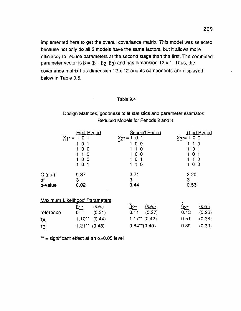
209

implemented here to get the overall covariance matrix. This model was selected

because not only do all 3 models have the same factors, but it allows more

efficiency to reduce parameters at the second stage than the first. The combinedparameter vector is ~ =(~1, ~2, ~3) and has dimension 12 x 1. Thus, the

covariance matrix has dimension 12 x 12 and its components are displayed

below in Table 9.5.

Table 9.4

Design Matrices, goodness of fit statistics and parameter estimates

Reduced Models for Periods 2 and 3

Q (gof)dfp-value

First PedodX1 * = 1 0 1,.,

1 0 11001 1 01001 0 1

9.3730.02

Second PedodX2* =1 0 1w 1 0 0

1 1 01001 0 1110

2.7130.44

Third PeriodX3*= 1 0 0,..

1 1 01 0 11 0 11 1 0100

2.2030.53

Maximum Likelihood Parametersl-

ll!.: (s.e.)reference 0 (0.31)tA 1.10** (0.44)

tB 1.21 ** (0.43)

,. ,.ll.2.: ~ ~ ~0.11 (0.27) 0.13 (0.26)1.17** (0.42) 0.51 (0.38)

0.84**(0.40) 0.39 (0.39)

** =significant effect at an a=0.05 level

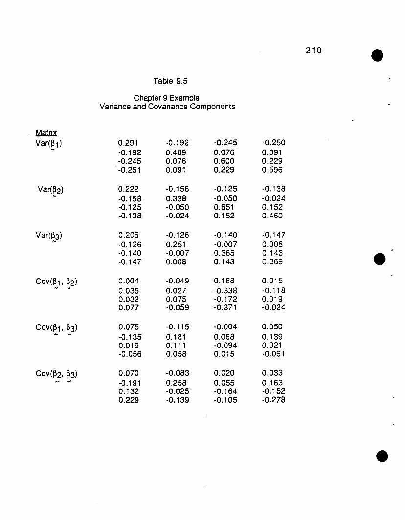
210

Table 9.5

Chapter 9 ExampleVariance and Covariance Components

MatrixVar(~1 ) 0.291 -0.192 -0.245 -0.250...

-0.192 0.489 0.076 0.091-0.245 0.076 0.600 0.229-0.251 0.091 0.229 0.596

Var(~2) 0.222 -0.158 -0.125 -0.138...

-0.158 0.338 -0.050 -0.024-0.125 -0.050 0.651 0.152-0.138 -0.024 0.152 0.460

Var(~3) 0.206 -0.126 -0.140 -0.147f'J -0.126 0.251 -0.007 0.008

-0.140 -0.007 0.365 0.143 e-0.147 0.008 0.143 0.369

COV(~11 ~2) 0.004 -0.049 0.188 0.015"-J '" 0.035 0.027 -0.338 -0.118

0.032 0.075 -0.172 0.0190.077 -0.059 -0.371 -0.024

COV(~11 ~3) 0.075 -0.115 -0.004 0.050"" '" -0.135 0.181 0.068 0.139

0.019 0.111 -0.094 0.021-0.056 0.058 0.015 -0.061

Cov(~21 ~3) 0.070 -0.083 0.020 0.033- "-J -0.191 0.258 0.055 0.163

0.132 -0.025 -0.164 -0.1520.229 -0.139 -0.105 -0.278

211

9,3,2 Second Stage Model Analysis

At this point Stram, Wei and Ware compare the effects across the periods with

a multiple hypothesis testing approach. Thus, comparing any two effects is done

relative to the appropriate covariance term between them. A more

comprehensive strategy is to do a second stage model with a weighted

regression, Thus the combined parameter vector is the function of analysis and

the combined covariance matrix is also required as input. If a 12 x 12 identity

matrix is applied to these effects, then the hypotheses summarized in Table 9,6

can be assessed.

Table 9.6

Hypotheses for Weighted Regression, Across PeriodsContrast fe) Null Hypothesis Q1. Qt1 000 -1 000000 01 000 000 0 -1 000 IJ. effects are equiv. 0,99 2

p-yalue

0.61

o1 000 -1 0000 0 0010000000-100

001000-10000000 1 00 0 0 0 0 0 -1 0

0001000-10000000 1 0000000 -1

It sq effects are equiv.

'tA effects are equiv.

'tB effects are equiv,

178,7 2

0.60 2

0,60 2

<0,0001

0.74

0,74

These hypotheses indicate that the intercept terms, the treatment A effects and

the treatment 8 effects are equivalent across the three periods. However, there

is a strong difference in the latin square effect. The following reduced model

implements these conclusions. The intercept and treatment effects are

smoothed across the periods and the latin square effects are modeled

separately for each period.XR =[ 1 0 0 0 1 0 0 0 1 0 0 0- o 1 0 0 0 0 0 0 0 0 0 0

o 0 000 1 0 0 0 0 0 0

o 0 0 0 0 0 000 1 0 0

001 000 1 000 1 0

000100010001]'

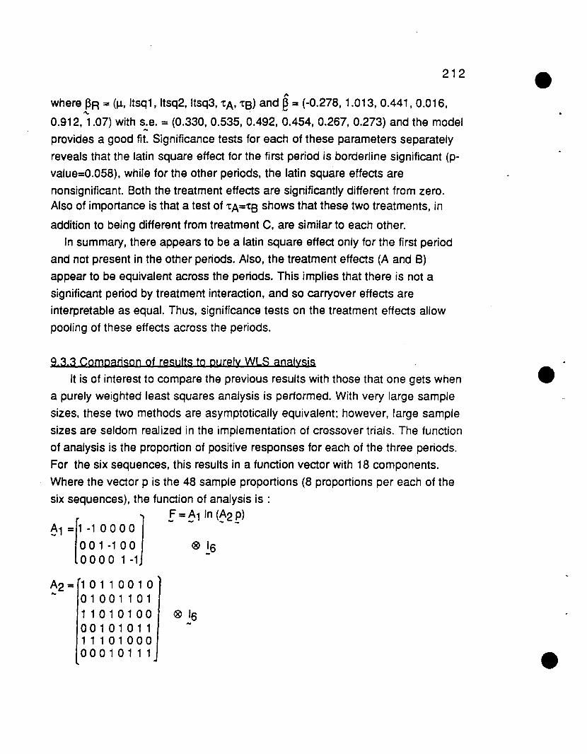
~1 =[1 -1 0 0 0 0 ]001 -1 000000 1 -1

212,..

where 13R = (J,J., Itsq1,Itsq2,Itsq3, tA, tB) and 13 = (-0.278,1.013,0.441,0.016,~ . ~

0.912, 1.07) with s,:e. = (0.330, 0.535, 0.492, 0.454, 0.267, 0.273) and the model

provides a good fit. Significance tests for each of these parameters separately

reveals that the latin square effect for the first period is borderline significant (p

value=0.058), while for the other periods, the latin square effects are

nonsignificant. Both the treatment effects are significantly different from zero.Also of importance is that a test of tA=tB shows that these two treatments, in

addition to being different from treatment C, are similar to each other.

In summary, there appears to be a latin square effect only for the first period

and not present in the other periods. Also, the treatment effects (A and B)

appear to be equivalent across the periods. This implies that there is not a

significant period by treatment interaction, and so carryover effects are

interpretable as equal. Thus, significance tests on the treatment effects allow

pooling of these effects across the periods.

9,3,3 Comparison Qf results tQ purely WLS analYsis

It is of interest to compare the previous results with those that Qne gets when

a purely weighted least squares analysis is performed. With very large sample

sizes, these tWQ methQds are asymptQtically equivalent; hQwever, large sample

sizes are seldQm realized in the implementation of crGssover trials, The functiQn

Qf analysis is the prQpQrtiQn Qf positive responses for each of the three periods,

For the six sequences, this results in a function vector with 18 components.

Where the vector p is the 48 sample proportions (8 prQportions per each Qf the

six sequences), the functiQn Qf analysis is :F = A1 In (A2 p)-..., """-

A2 = 1 0 1 1 0 0 1 0... 01001101

1 1 0 1 0 1 0 0 ~ 16001010111110100000010111

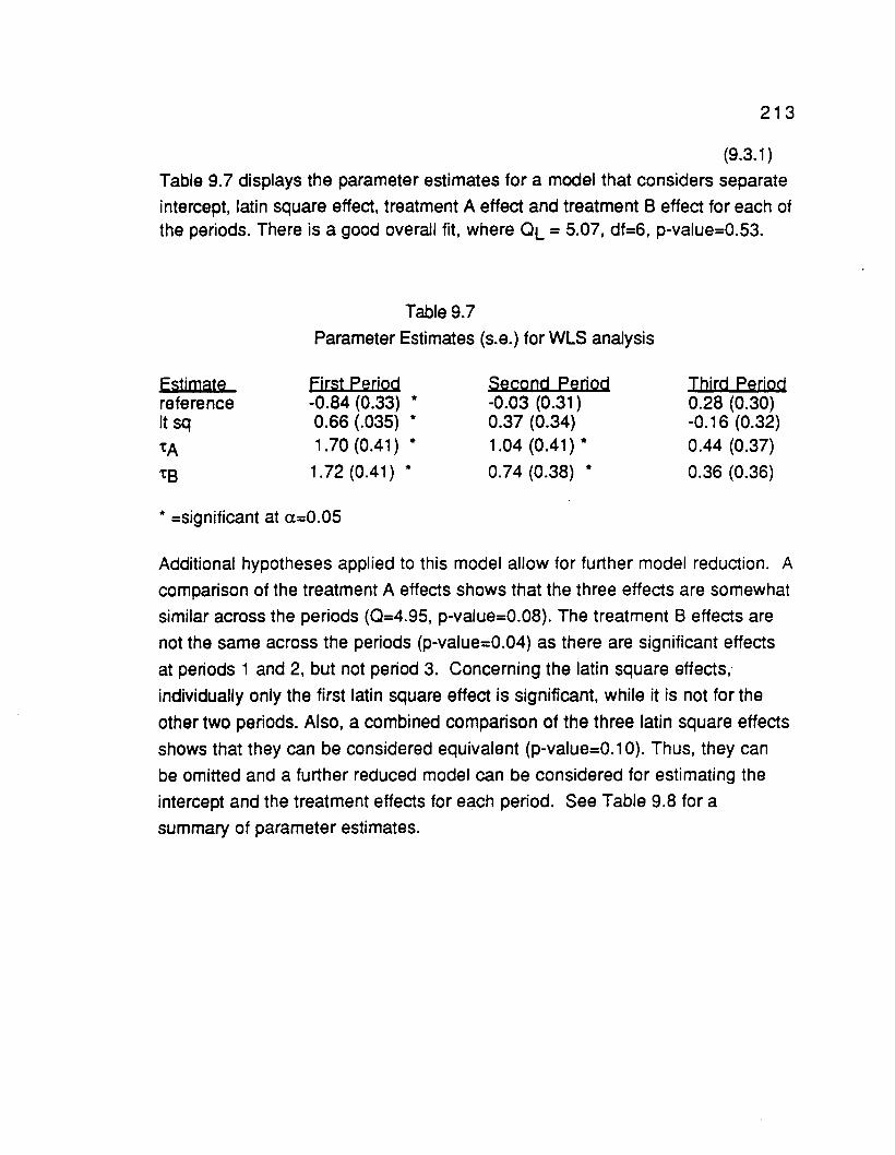
213

(9.3.1 )

Table 9.7 displays the parameter estimates for a model that considers separate

intercept, latin square effect, treatment A effect and treatment B effect for each ofthe periods. There is a good overall fit, where 0L = 5.07, df=6, p-value=0.53.

Table 9.7

Parameter Estimates (s.e.) for WLS analysis

EstimatereferenceIt sq

tAtB

First Period-0.84 (0.33) •0.66 (.035) •1.70 (0.41) •

1.72 (0.41) •

Second Period-0.03 (0.31)0.37 (0.34)1.04 (0.41) •

0.74 (0.38) •

Third Period0.28 (0.30)-0.16 (0.32)0.44 (0.37)

0.36 (0.36)

• =significant at a=0.05

Additional hypotheses applied to this model allow for further model reduction. A

comparison of the treatment A effects shows that the three effects are somewhat

similar across the periods (0=4.95, p-value=0.08). The treatment B effects are

not the same across the periods (p-value=0.04) as there are significant effects

at periods 1 and 2, but not period 3. Concerning the latin square effects,

individually only the first latin square effect is significant, while it is not for the

other two periods. Also, a combined comparison of the three latin square effects

shows that they can be considered equivalent (p-value=0.1 0). Thus, they can

be omitted and a further reduced model can be considered for estimating the

intercept and the treatment effects for each period. See Table 9.8 for a

summary of parameter estimates.

214

Table 9.8

Parameter Estimates (s.e.) for WLS analysis, Reduced ModelEstimate First Period Second Period Third Periodreference -0.52 (0.28 * 0.18 (0.26) 0.21 (0.25)'tA 1.64 (0.40) * 1.05 (0.41) * 0.37 (0.36)

'tB 1.78 (0.41) * 0.67 (0.38) ** 0.25 (0.36)

* =significant at a=0.05** = borderline significant with p-value=0.08

The overall fit of the model is good (0=11.48, df=9, p-value=0.24). Similar

conclusions with regards to treatment significance still hold. Treatment A effects

are only borderline equivalent (p-value=0.08) and the treatment B effects are

different from each other (p-value=0.02). This implies that there is a significant

carryover contribution since there appears to be a treatment by period

interaction. One could conclude that the carryover due to treatment B is stronger

than that attributable to treatment A.

Both the Stram, Wei and Ware and purely WLS results are primarily in

agreement at a period specific level. Note that while the parameter values are

slightly different in Table 9.3 vs Table 9.7 and Table 9.4 vs Table 9.8, they agree

in magnitude and significance. Both approaches find a latin square effect only

in the first period. Both find significant treatment effects in periods 1 and 2, but

not period 3. Further reduced models corresponding to the stage two with

Stram, Wei and Ware's covariance show some differences. The first method

suggests no carryover effects, and similarities of treatments A and B. The WLS

approach revealed that potential non null carryover may exist especially for the

treatment B (since the treatment B effect appears to differ across the periods).

This later method agrees more closely with the results from the Gart method

presented in Chapter 5 for the same data using only the discordant outcomes.

In that example, it was concluded that while there were no latin square effects,

there were significant period, treatment and carryover effects.

215

9,314 Comparison to results to Bonney type of seQuential modeling

As presented in Chapter 2, Bonney (1987) considers a method of sequential

modeling where the models would be for just period 1 (first order marginal table

as with the Stram, Wei and Ware method), period 2 conditioned on the period 1

outcome, and period 3 conditioned on the responses at periods 1 and 2, These

results are summarized in Table 9.9.

From these models, a variety of conclusions are evident. The Latin square

effect exists only for the first period. This agrees with the result of the previous

two methods. Also in agreement with the other two approaches is the fact thatboth treatment A and B effects ('tAl 'tB) are significant in all models for periods 1

and 2. The difference that this sequential approach suggests is that for period 3

conditioned on periods 1 and 2, there are significant treatment effects. Also,

there is a significant period 2 effect. While the particulars of the models differ,

they generally agree in conclusions of relationships and magnitude of

parameter estimates. The main difference being that the sequential period 3

model reveals that the treatment effects can be significant when the other

periods are controlled. This is suggestive of a period by treatment interaction,

Table 9.9

Results from Bonney type of Sequential Modeling1$t Period 2nd Per I Period 1 3rd Per I Periods 1 and

2a (gof)dfp-value

3.3220.19

5.9270.55

16.01180.59

~0.89 (0,37) *

-0.70 (0.36)-1,59 (0,37) *-0.33 (0.35)0.81 (0.41) *

0.78 (0.43) *

0.37 (0.34)1,20 (0.44) *

0.84 (0.41) *

0.89 *1.10*

1.19 *

Maximum Likelihood Parameters (s,e,)

.al .am-0.38 -0.03 (0.32)

-0.20 ( 0.37)mean (J.1)P1 (#)P2 (##)latin square

'tA

'tB

* = significant effect at an 0.=0.05 level# = Period 1 effects are defined only for periods 2 and 3## = Period 2 effects are defined only for period 3

216

9.4 Other potential covariance calculations

There are other possible covariance methods that can be considered to

account for association present across the correlated period responses. These

will be briefly considered in order to display the broad scope that these type of

estimates can encompass.

Stram, Wei and Ware present a general covariance matrix that has desirable

properties for estimation; but as a result, the variance component for any single

period is slightly different than that one would ordinarily arrive at with a direct

principles approach with maximum likelihood principles.

With a direct principles approach to calculate the variance at the j-th period,

the following equation eXists. For

" ""0.. = diag { n, e " (1 - e " )}~ JJ 1 IJ IJ

Vj is the variance matrix for the parameter vector for j-th period as follows :

" • 1Var {/3 ,} = (X.' 0 .. X . )

_ J _ J _ JJ _ J

(9.4.1 )For the parameter vector combined across all periods: /3 = (/31, ... , /3d)

The overall covariance matrix is :

"Var (/3) = V X' 0 X V

where

217

0 0 0.. 11 -12 -ld

o = 922 P2d"-

symmetric :'cij

andPH' = diag { nj ( Sijj' - Sjj Sij' )} for j *" j',

(9.4,2)'!. and ~ are block diagonal matrices with Yj and 2<j in the block structures,

respectively. Thus the problem is to estimate the undetermined quantity

Sijj' = E {Yijk Yjj'k}

A brief summary of three potential alternate strategies are as follows:

Strategy 1 - Based on cell counts:Pjj' = diag { (aid i - bjCi) I nj }

S"'lj'j" a'/n'= , I, 8"ij' = (aj + cj)/nj, 8" ij = (ai + bj)/n i ,

Strategy 2 - Cell Counts and Model-based :

""a .. =

IJ

exp (2<' i ~ i ), "

1 + exp (X . ~. )- J - J

Sijj' = aj I nj

'pjj' = diag { nj (aj/nj - S"jj S"ij') }

Strategy 3 - All Model-based Estimates :Sijj' = exp { X'jj'~} I [1 + exp { X'jj'~ } ]- -

logistic modeling for the binary outcome variable W :

218

W = 1 if the response is positive for both times j and j' (aj cell)

W = 0 otherwise

Note how these differ from the covariance term proposed by Stram, Wei and

Ware of equation (9.2.4). With their calculation,

Oil' =""

While their estimated covariance matrix provides a good estimate, it remains to

be seen how this compares to other proposed strategies.

9.4.1 Simulation to compare variance component

A simulation study was undertaken to illustrate the differences in period

specific variance calculations between the Stram, Wei and Ware method and

the usual maximum likelihood method. This simulation will show that for the

specific data situation of case record observations (Le. one or at most few

subjects in each subpopulation), the variance corresponding to the parameters

at just one visit will be somewhat different for the two methods.

The example used to illustrate this conclusion is a bioassay-like example for

one time period and one subpopulation. Three separate simulation studies

were undertaken each with 500 repetitions. For the first simulation, one

repetition involves n=21 subjects with unique data points specified by x = -2.0, -

1.8, .... 2.0 (incremented by 0.2). These are the descriptive "covariate"measures. From these the predicted probability 8i=eXi / (1 + eXi) is calculated.

For each subject, a uniform (0,1) random variable is generated. If this random

variable is greater than that probability, then the outcome y=O, otherwise y=1.The probability that this random outcome y is a positive event (value=1) is

associated with the logistic function such that as the x covariate values

increase, the likelihood of a positive outcome increases. Thus, the logistic

regression situation has been created for the binary outcome.

219

From this specification, the true parameter values are intercept ~O=O and the

slope J31 =1. The formula for the true variance is

Var(~) = ( X' diag (8j (1-8i) ) X ) ·1 based on the predicted probabilities 8i. The'" OJ "'"

true variance values for the first simulation where n=21 subjects is :

f0.2557 0 1o 0.2269

For n=41 subjects

l 0.1295 0 Jo 0.1192

and for n=81

[0.0652 0 ]o 0.0611

From this data array, a logistic regression of yon x is performed and ML

iteration is done to estimate the intercept and slope parameters. Also,

calculated for each of the repetitions is

~= exp (~~ / ( 1 +exp(~ID )Var(@j = (~ diag (8i (1-6i) ) ?5 ) ·1

Var(IDsww = (X' diag (Yi - 2Yi 8j + 8i2) X ) -1~ -

Means and variances across the N=500 repetitions are summarized in Table9.10 for the following six quantities: the intercept ~Ol its variances by the usual

method and by the Stram, Wei and Ware method, the slope ~11 and its

variances by the usual and Stram, Wei and Ware's methods. Also shown in this

table are the two other simulation studies which both increased the overall

sample size. Simulation 2 is based on n=41 for x=-2, -1.9, ... 2 (by .1

increments). Simulation 3 uses n=81 with x=-2, -1.95, .... 2 ( by .05

increments). 80th were done with N=500 repetitions.

The summary statistics presented in Table 9.10 for n=21 and n=41 are based

on the subset of data arrays with parameter vectors whose values fall within 4 or

5 standard deviations, respectively, based on the true variance calculation. For

220

n=21 subjects, 427 repetitions were used as those within 4 standard deviations.

For the n=41 simulation study, 463 repetitions were used as those falling within

5 standard deviations. This excluded those individual experiments which were

so deviant that if found in practice one would not proceed with these methods

because the results are obvious or irrelevant a priori. For the n=81 simulation

study, the number of sUbjects for each repetition was large enough that the

random vectors assigned to each of the repetitions did not yield any

experiments with estimated parameters outside 5 standard deviations. Note that

in all 3 simulation runs, the variance calculation from the ordinary maximum

likelihood method (averaged across repetitions) is closer to the true variance

calculation than the Stram, Wei and Ware method, although not statistically so

relative to their variance. Furthermore, paired ttests on the difference of theusual variance of ~O (or ~1) minus the Stram, Wei and Ware variance of ~O (or

~1) revealed that these two differences are significantly less than zero (all p-

values for ttests are <0.001). This is true for all three simulation studies where

the Stram, Wei and Ware variance is always larger than the usual variance and

thus further from the asymptotic variance. Thus, there is sufficient evidence to

assert that the period specific variance formula of Stram, Wei and Ware does

not perform as well relative to the intuitive and standardly implemented variance

calculation with maximum likelihood methods for logistic regression. What

happens for covariance terms remains to be investigated, but these results

suggest that properties may be reasonable in moderately large samples but

subject to some discrepancy.

Table 9.10Simulation Study

Comparing Stram, Wei and Ware Method vs Usual Method

Sim

n=21

n=41

n=81

Number of Est. Params asymptotic -----------Mean (Var) ------------

Reps Variance Usual SWWjill li \'arffiO) Yar(fil) Var(BO) Yar(fil) . Var(fiO) Var( fi 1 )

N=427 * -0.006 1.024 0.256 0.227 .297(.001) .274(.013) .337(.028) .340(.049)

N=463 + -0.008 1.049 0.130 0.119 .142(.001) .136(.002) .147(.001 ) .146(.003)

N=500 -0.026 1.049 0.065 0.061 .069(.0001) .068( .00(4) .071 (.0001) .071(.0006)

* = based on repetitions within 4 standard errors of the true parameter vector+ = based on repetitions within 5 standard errors of the true parameter vector

I\)I\)-"

222

CHAPTER 10

MODELS FOR THREE PERIOD CROSSOVER DESIGNS

FOCUSING ON PAIRWISE PERIOD RATIOS

10,1 Introduction

The goal of Chapter 10 is to present another strategy for the crossover

design, The focus is still on the discordant joint outcomes where the effects are

defined in terms of the subject specific, marginal probabilities. The strategy will

be referred to as the pairwise period ratio method due to its reliance on ratios

of responses from pairwise combinations of periods.

This method will be considered in detail for the three period crossover stUdy

with a binary response but will be appropriate for more complicated designs. A

weighted least squares analysis will be used for these ratios. The possibility of

collinearity among these ratios will be addressed with a smoothing applied to

the functions of analysis.

Thus, Section 10.2 will consider a different function as the focus of analysis

for the three period cross over design. Section 10.3 explores the extension to

nominal and ordinal outcomes while Section 10.4 considers higher order

designs. Missing data extensions are presented in Section 10,5. An example is

presented in Section 10.6 followed by a discussion.

10.2 Strategy for analyzjng pairwise period ratios for the three period binary

crossover study

223

Consider the three period crossover design where subjects are randomly

assigned to one of six sequence groups: A:B:C, B:C:A, C:A:B, A:C:B, C:B:A and

C:A:B. For the binary response outcome, the subject-specific, marginal

probabilities in Table 5.1 will still be applicable. The period, treatment and

carryover effects are interpreted relative to these probabilities. These are the

same marginal probabilities employed in Gart's method. Again, the conditional

independence assumption means disregarding the two concordant

observations (000) and (111).

For each of the sequences the following three ratios will be considered. The

first of these will be called (P3-P2) effect and will, in a sense, sum the number

of responses across period 1 in order to compare periods 2 and 3 with a ratio

estimate. The comparison is made relative to the (10) response for periods 2

and 3 vs the (01) response. This ratio quantity is displayed below:

(P3-P2) effect =Pr (Yi1 =0, Yi2=1, Yi3=0) + Pr( Yi1 =1, Yi2=1, Yi3=0)

= [(001) + (101)] / [(010) + (110)]

(10.2.1)

Similarly for the the effect summed across period 2 which compares the period

1 with respect to period 3 :Pr (Yi1 =0, Yi2=0, Yi3=1) + Pr( Yi1 =0, Yi2=1, Yi3=1)

(P3-P1) effect =

= [(001) + (011)] / [(100) + (110) ]

(10.2.2)

And for the comparison of periods 1 and 2 :Pr (Yi1 =0, Yi2=1, Yi3=0) + Pr( Yi1 =0, Yi2=1, Yi3=1)

(P2-P1) effect =

224

=[ (010) + (011)] / [(100) + (101) ]

(10.2.3)

For the first of the six sequence groups composing this three period crossover

design, Table 10.1 indicates the probabilities associated with these ratios

based on the marginal probabilities displayed in Table 5.1. Accordingly,

parameters have the same definition as already provided. For the sequence

group A:B:C, the specifics of one of the calculations are shown below.

(P3-P2) effect = [(001) + (101)] / [(010) + (110)]= [exp(CLk+1t3+AB} + exp(2CLk+1t3+tA+AB] / g1 (CL,1t,t,A) +

[exp(CLk+1t2+tB+AA) + exp(2CLk+1t2+tA+tS+AA] / g1 (CL,1t,t,A)

=exp(1t3+AS) (1 + exp(CLk+tA)) / exp(1t2+tB+AA) (1 + exp(CLk+tA) )

=exp(1t3 + AB) / exp(1t2 + tB + AA)

(10.2.4)

Table 10.1

Pairwise period ratiosA:B:C (P3-P2) ratio exp(1t3 - 1t2 - tB - AA + AS)

(P3-P1) ratio exp(1t3 - tA + AB)

(P2-P1) ratio exp(1t2 - tA + tB + AA )

Notice the relationship that exists between the asymptotic expected values of

these ratios.

In (P3-P1 ) ratio - In (P2-P1) ratio = In (P3-P2) ratio

(10.2.5)

More importantly, notice that for any sequence, these three ratio estimates are

correlated with each other. Out of the six discordant joint outcomes, any two of

the ratios share two of their four discordant components in common. For

instance, the (P3-P2) effect and the (P3-P1) effect share the outcome (001) in

the numerator and the outcome (110) in the denominator. This relationship can

more graphically be displayed with the following Table 10.2.

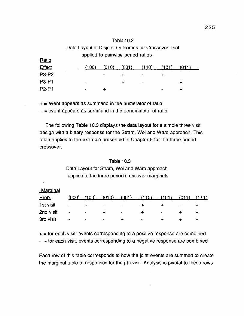
225

Table 10.2

Data Layout of Disjoint Outcomes for Crossover Trial

applied to pairwise period ratiosBatiQ

Effect (100) (010) (001 ) (110) (101 ) (011 )

P3-P2 + +

P3-P1 + +

P2-P1 + +

+ = event appears as summand in the numerator of ratio

- = event appears as summand in the denominator of ratio

The following Table 10.3 displays the data layout for a simple three visit

design with a binary response for the Stram, Wei and Ware approach. This

table applies to the example presented in Chapter 9 for the three period

crossover.

Table 10.3

Data Layout for Stram, Wei and Ware approach

applied to the three period crossover marginals

Marginal

~ (000) (100) (010) (001) (110) (101 ) (011 ) (111 )

1st visit + + + +

2nd visit + + + +

3rd visit + + + +

+ =for each visit, events corresponding to a positive response are combined

- =for each visit, events corresponding to a negative response are combined

Each row of this table corresponds to how the joint events are summed to create

the marginal table of responses for the j-th visit. Analysis is pivotal to these rows

226

and the overlapping nature of this table indicates the correlated structure

present in the parameter estimates.

Note that while the two Tables 10.2 and 10.3 differ with respect to the basic

function of analysis, they share the same feature of correlation across these

functions. Stram, Wei and Ware and other methods for population marginal

analyses estimate the probabilities from each of the marginal tables separately

and then provide an estimate of the covariance across these tables, taking into

account this correlation.

Consider for the three period crossover design the following three tables, let

ni(yi1, yi2, yi3) represent the number of patients in the i-th sequence group with

the response (Yi1, Yi2, Yi3). Then Table 10.4 represents the cell counts of the

Tables used for each of the three separate logistic models.

~

P3-P2.5J!.gA:B:C

B:C:A

Table 10.4

Tables of cell counts for Analysis

Table 1 LQ.lln1(001) + n1(101)

n2(001) + n2(101)

lliUn1(010) + n1(110)

n2(010) + n2(11 0)

P3-P1

P2-P1

Table 2 LQ.ll lliUA:B:C n1(001) + n1(011) n1(100) + n1(110)

B:C:A n2(001) + n2(011) n2(100) + n2(11 0)

......Table 3 LQ.ll illll

A:B:C n1 (010) + n1 (011) n1(1 00) + n1(1 01 )

B:C:A n2(010) + n2(011) n2(100) + n2(1 01)

Notice that for all the pairwise ratios, each table compares the 01 vs 10

discordant responses. These are the outcomes of focus depicting those who

have a preference between the two periods, which are the essential

components of Gart's method for two sequence groups with two periods.

227

From the first of these tables of counts, a logistic model functioning on the

logits in effect evaluates the P3-P2 differences for each of the sequences. For

the sequence A:B:C, the logit for this effect is In(P3-P2 effect). Table 10.5

displays the logits for each of the ratio models for each of the sequences along

with the associated design matrix. Each of these design matrices will bereferred to as XP3-P2, XP3-P1 and Xp2-P1, respectively.

'" '" -

Model1

Table 10.5

Logits and design matrix for each ratioRatio Effect Seguence . J..QgllP3-P2 A:B:C 1t3-1t2-'tB-AA+AB

B:C:A 1t3-1t2+'tA-AB

C:A:B 1t3-1t2-'tA+'tB+AA

A:C:B 1t3-1t2+'tB-AA

C:B:A 1t3-1t2+'tA-tB+AB

B:A:C 1t3-1t2-tA+AA-AB

Design Matrix1 0 -1 -1 1

1 1 0 0 -1

1 -1 1 1 0

1 0 1 -1 0

1 1 -1 0 1

1 -1 0 1 -1

2 P3-P1 A:B:C 1t3-tA+AB

B:C:A 1t3+tA-tB

C:A:B 1t3+tB+AA

A:C:B 1t3-'tA+tB

C:B:A 1t3+tA+AB

B:A:C 1t3-tB+AA

1 -1 0 0 1

1 1 -1 0 0

1 o 1 1 0

1 -1 1 0 0

1 1 001

1 o -1 1 0

3 P2-P1 A:B:C 1t2-'tA+tB+AA 1 -1 1 1 0

B:C:A 1tZ-'tB+ AB 1 0 -1 0 1

C:A:B 1t2+tA 1 1 0 0 0

A:C:B 1t2-tA+AA 1 -1 0 1 0

C:B:A 1t2+tB 1 0 1 0 0

B:A:C 1t2+'tA-tB+AB 1 1 -1 0 1Notice for the first model, the 5 degrees of freedom that are modeled are ~P3-

'""P2 = (O=7t3-1tZ, tA, tB, AA' AB)" The other models incorporate a slightly

different component of the period effect in addition to treatment and carryover

and

228

effects; in this regard, ~P3-P1 = (1t3, 'tA, 'tB, A.A, A.B)'-includes 1t3 and ~P2-P1 =- -(1t2, 'tA, 'tB, A.A' A.B)' includes 1t2·

For the estimates across the pairwise period ratios, there exists a covariance

because of correlated logits. A weighted least squares analysis can be applied

which accounts for this correlation through the appropriately defined functions

F....Let F = A2 In A1 p

where - A1 = 0'" 0""1 0 1 0.... 010100

o 0 1 0 0 1 ~ IS100 1 0 0 ~

o 1 000 11 0 000 1

~211 -1 0 0 0 0]o 1 -1 0 0 ~ ~S

o 0 0 1 -1

then F expresses the logits associated with the pairwise period ratios.-Let ~ = ( 0=1t3-1t2, 'tA, 'tB, A.A, A.B, 1t3, 'tA, 'tB, A.A' A.B, 1t2, 'tA, 'tB, A.A, A.B)' be

the combined vector of parameters; then each ratio has its own set of estimates.

After appropriate hypothesis tests, it may be possible to combine these

parameters across the ratios.For instance, the test HO: C~=O where...... ""C = ( 0 1 000 0 -1 000 00000- o1 000 00000 0 -1 000 )compares the equivalences of 'tA effects across the pairwise period ratio.

Acceptance of such a hypothesis implies an average of the 'tA effects may be

appropriate across the three models. As already explained, the threeparameter vectors estimate different components of period effects o=1t3 - 1t2,

1t3, and 1t2, respectively; this must be handled somewhat differently. One could

test that HO:0=1t3-1t2 via C = ( 1 0000 -1 00 00 1 0000 ). When it is not,..

appropriate to combine the estimates across the pairwise period ratio model, a

primary effect by pairwise period effect interaction may be indicated. In otherwords, if the 'tA's cannot be combined, then the treatment A effect varies for the

pairwise period combinations. This treatment by pairwise period ratiointeraction implies a type of carryover effect might be present beyond the A.

229

effects which are direct treatment by period interactions. Interpretation of these

interactions may not be obvious.

A further note of interest is that if only one Latin square is applied to the

design, then only three sequences would be used. As a result, one can only

estimate period and treatment effects, but not the carryover effects. When both

Latin squares are applied to these models then each has 5 degrees of freedom

when the design is that of Table 10.5. The remaining degree of freedom

corresponds to the Latin square effect.

Weighted least squares analysis requires large enough sample size. Unless

there are lots of O's and 1's in the cell counts, then WLS is feasible. Particularly

as these pairwise period ratios combine joint counts, this aggregate

information lends more sample size to the function for analysis. The type of

ratio structure and model discussed here has not been discussed before by

any analysis strategy; thus despite sample size, WLS is an appropriate

beginning.

The redundancy among the asymptotic expected values was displayed in

equation 10.2.5. While collinearity may not exist in finite samples, the

possibility of near collinearity among the ratios as the sample size increases

needs to be considered. This can be examined informally by a synthetic

example where all cell counts are greater than 5. See Table 10.6 for a display

of the data. Ignoring the potential collinearity, regression of one column of the

covariance matrix of the ratios on the other two columns yielded R2 in the

range of 0.91 to 0.96 (by sequences). Because of this concern of approaching

collinearity, a method will be proposed which involves an ordinary least

squares smoothing applied to the functions.

230

Table 10.6

Synthetic Example to look at collinearity

~ UQQl !Q.1Ql LQ.O.1l illQl Ll.O.ll !Q..l1l

ABC 8 9 5 12 9 6

SCA 5 11 10 5 11 7

CAB 8 5 11 8 12 12

ACB 9 8 10 6 8 11

CBA 6 7 8 12 8 9

BAC 11 7 9 9 13 15

From equation 10.2.5, the constraint (-1 1 -1 )' applies for each set of three

ratios. The orthogonal matrix to this involves two columns (1 1 0)' and (0 1 1)'.

Fittini ~h[~ doejSign matrix

,.. ~ ~ ®!6

to the ratio functions F, provides the estimates G = (X' Xt 1 X' F, reducing the,..., aJ ~ N --

number of estimating functions from 3 to 2 per sequence. These functions are

the cell means for the first and third function, smoothing across the redundancy

that exists with the second. Then a new model corresponding to the (P3-P2)

and (P2-P1) structure for the smoothed G functions is applied. In this way,,..asymptotic redundancy is avoided. Section 10.6 will further address both of

these strategies in an example.

10.3 Ratio method extended to nominal and ordinal outcomes

When one considers a crossover design involving an ordinal response, this

ratio method of comparing pairwise periods can still be applied for the three

period design. Considering the categorical response with three outcomes

(R=3), there are 24 discordant joint probabilities to consider out of 27 possible

joint outcomes. The outcomes (111), (222) and (333) are excluded from

analysis. Table 5.6 in Chapter 5 displays the marginal probabilities from which

231

these 24 joint probabilities are obtainable. Comparison of periods 2 and 3 with

a ratio which sums across period 1 involves three separate ratios which

compare response 1 vs 2, responses 1 vs 3 and responses 2 vs 3 (Le. (21) vs

(12), (31) vs (13) and (32) vs (23)). Shown below is the structure for these

ratios.

(P3-P2) ratio for response 1 vs 2 =

[(112) + (212) + (312)] / [(121) + (221) +(321)]


[(113) + (213) + (313)] / [(131) + (231) +(331)]


[ (123) + (223) + (323)] / [(132) + (232) +(332)]

The corresponding sets of three ratios can similarly be created for periods 1 vs

2 summing across the period 3 responses and for periods 1 vs 3 summing

across the period 2 responses. Subsequently, three separate models for each

of the period ratios become of interest. Each model involves three ratios for

each sequence group. Thus, if there are six sequence groups, the design

matrix for the (P3-P2) effect has 18 rows modeling 10 degrees of freedom for

02=7t32-1t22, 03=7t33-1t23, tA2, tA3, tB2, tB3, AA2, AA3, AB2,and AB3 as the

parameters of interest. The other two models for P3-P1 effect and P2-P1 ratio

also have 18 rows in their corresponding design structure. As consistent with

Chapters 3 and 4, an equal adjacent odds ratio assumption implies a

restriction on the parameters which allows incorporation of the ordinality of theresponse. Thus, each ratio model can consider 5 parameters as follows o=1t3

1t2, tA, tB, AA and AB. The restrictions with this assumption for the treatment A

effect, for instance, are tA2 = tA and tA3 = 2 tAo Similar WLS analysis applies

as in Section 10.2 where consideration for the redundancy among ratios can

be addressed with the smoothing technique.

10.4 Higher Order Designs

This approach has the advantage of extensions to higher order designs. The

same principles apply for any number of periods and for any number of

treatments for the binary outcome. For example, with the four period design,

there are 14 discordant sets representing the joint outcomes of focus. One

232

sums the counts across two of the periods in order to compare the other two

periods. Thus, for each sequence, there are six comparisons of interest. These

involve comparing the 01 vs 10 outcomes for periods 1 vs 2, periods 1 vs 3,

periods 1 vs 4, periods 2 vs 3, periods 2 vs 4, and periods 3 vs 4. The last

comparison will illustrate this calculation. Summing across periods 1 and 2, the

comparison of periods 3 and 4 discordant pairs is :

(P3-P4) ratio =[(0001) + (0101) + (1001) + (1101)] / [(0010) + (0110) + (1010) + (1110)].

Thus, each of these six pairwise period ratios corresponds to its own model.

From here, analysis proceeds as it did in Section 10.2.

When four periods are investigated with a crossover design where an ordinal

response has been observed, the use of this method can still be implemented

with the same algorithm of taking ratios. For the four period design with R=3

response categories, there are 6 models each with three ratios per sequence

group. The sample size must be sufficient to handle the magnitude of this

problem.

10.5 Unobserved Outcomes

A further advantage of this procedure is that when not all of the joint

responses have been observed, one can still calculate an estimate of pairwise

period ratios by omitting the response that was not observed. When a joint

response is not observed this implies a zero count for that outcome. For

instance, if the outcome (0001) was unobserved in the population for the 4

period design with a binary response, then the P4-P3 ratio would proceed to

sum three instead of four quantities in the numerator. The presence of zero

counts creates a problem only when the unobserved outcomes are so

prevalent that all 4 counts in either the denominator or the numerator are

unobserved.

A further issue for missing data occurs if a particular period is unobserved for

a particular sequence group or subject. For instance, if a subject contributes

data only for periods 1 and 3, then the (P3-P1) ratio can be estimated by

comparing those subjects with a (01) in periods 1 and 3 vs those subjects with

a (10) response in these two periods. It is still possible to compare period 3 and

233

1 via this ratio because the counts are summed across period 2. Thus, period 2

does not contribute information to this ratio. However, one cannot compare

period 1 vs 2, or period 2 vs 3 for the subject with missing period 2 data.

10.6 Example

The same example that was used in Chapters 5 and 9 will again be

presented here to illustrate the pairwise period ratio method. As before, there

are three periods, where patients are assigned randomly to the six sequence

groups to evaluate three treatments for the presence or absence of a condition.

Refer to Table 5.16 for the data counts displayed by the joint outcomes. Table

10.7 displays the numbers of subjects comprising each of the comparisons for

the three different models. Note however that modeling is performed relative to

the joint counts of Table 5.16.

A model with appropriate period effects and treatment and carryover effects

for each of the pairwise period ratios, as displayed in Table 10.5, is used to

arrive at WLS estimates for the parameters. This model is considered

regardless of potential collinearity. Note that zero cells are replaced with 0.5 for

estimation to occur. From this block diagonal design structure, the estimates for

these are shown in Table 10.8. The goodness of fit of this model is supportedwith QW=2.69, df=3, p-value=0.44.

Table 10.7

Three period, three treatment, binary response example

234

235

Table 10.8Parameter estimates and gof statistics, full model

Model Parameter Estimate ~P3-P2 effect

1t3-1t2 0.413 0.298

tA -0.870 0.495 +

t8 -0.972 0.514 +

/...A 0.115 0.489

/...8 -0.332 0.477

P3-P1 effect

1t3 1.109 0.560 ..tA -1.084 0.382 ..

t8 -1.082 0.466 ..

/...A -1.399 0.713 ../...8 01.511 0.718 ..

P2-P1 effect

1t2 -0.388 0.557

tA -0.827 0.426 ..

t8 -0.711 0.396 +

/...A 0.011 0.812

/...8 0.005 0.805

.. = significant of <l=0.05

+ = borderline significant at 0.05 < a < 0.10

Hypothesis tests are undertaken to see if any of the similar type parameterscan be combined across the ratio measures. All tests of HO:CJ3=O were-,.. ""nonsignificant (all p-values > 0.15), thus there is no distinction between similar

effects based on the three ratios. Since the carryover effects are nonsignificant

in the first and third models and the 2 degree of freedom test for carryover

effects equivalent is supported, a reduced model will be assessed for only

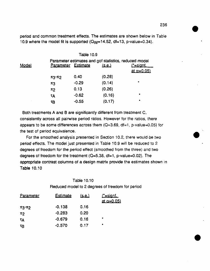
236

period and common treatment effects. The estimates are shown below in Table10.9 where the model fit is supported (OW=14.52. df=13. p-value=0.34).

Model

Table 10.9

Parameter estimates and gof statistics, reduced modelParameter Estimate ~ '-=signf.

at a=0.05)0.40

-0.29

0.13

-0.62

-0.55

(0.28)

(0.14)

(0.26)

(0.16)

(0.17)

-*

*

80th treatments A and 8 are significantly different from treatment C,

consistently across all pairwise period ratios. However for the ratios, there

appears to be some differences across them (0=3.69, df=1, p-value=0.05) for

the test of period equivalence.

For the smoothed analysis presented in Section 10.2, there would be two

period effects. The model just presented in Table 10.9 will be reduced to 2

degrees of freedom for the period effect (smoothed from the three) and two

degrees of freedom for the treatment (0=5.38, df=1, p-value=0.02). The

appropriate contrast columns of a design matrix prOVide the estimates shown in

Table 10.10

Table 10.10

Reduced model to 2 degrees of freedom for period

Parameter Estimate 1.sJW

7t3-7t2 -0.138 0.16

7t2 -0.283 0.20

'tA -0.679 0.16

't8 -0.570 0.17

(--sign!'at a-0.05)

*

*

237

Furthermore, the smoothed analysis of Section 10.2 could be implemented.

The redundancy among the ratios can be smoothed to consider P3-P2 andP2-P1 resulting in estimates for 1t2, 1t3-1t2 and the two treatment and two

carryover effects.

10.7 Discussion

In summary, an alternate strategy was presented which uses the Gart type

subject-specific marginal probabilities as a basis in order to estimate treatment,

period and carryover effects. This strategy differs from the strategy of Chapter 5

for the three period crossover which represents a pure Gart type extension to

assess the relationship between the six discordant joint outcomes.

The proposed strategy of this Chapter also arises from the Gart strategy, but

proceeds to observe pairwise period ratios. This strategy also provides

estimates for the period, treatment and carryover parameters. However, the

dependency parameters are not obtainable as not enough degrees of freedom

are available in the three period crossover design to estimate these. This

strategy is easy to implement and interpret as, well as allowing obvious

extensions to higher order designs for the binary response.

It can also be extended to the nominal outcome or the ordinal outcomes with

the equal adjacent odds ratio model. With sufficient sample size, higher order

designs with ordinal outcomes can still be analyzed with the pairwise period

ratios. The inclusion of covariates into the study design is forthright and one

can proceed to encompass either categorical or continuous covariates as

presented in Chapters 3 and 4.

In conclusion, for 3 period and higher order crossover designs with the binary

or ordinal outcome, the pairwise period ratio method has the advantages of

straightforward interpretation, ease of use and can handle missing data.

However, it does not allow for assessment of dependency parameters, as does

the Gart type extension.

The weighted least squares method was presented as the analysis strategy

with a smoothing method developed to adjust for potential asymptotic

collinearity. Another method to be developed in future research is to consider

238

the two stage method of Stram, Wei and Ware (1988). At the first stage, each of

the ratios is modeled separately with logistic regression. Then the Stram, Wei

and Ware approach is used for estimation of covariance across ratios. One

major consideration in this is how to adjust for the sample size which varies for

each of the ratios. Also, consideration of redundancy among the ratios

becomes more complicated where any type of smoothing must be incorporated

through the covariance structure.

239

CHAPTER 11

SUMMARY AND FUTURE DIRECTIONS

11 ,1 Summary

Many of the strategies designed to handle categorical data from the

crossover design are limited in focus to only the two period, two treatment trial

for the binary response. There is a need to have methods that allow for a

response to be nominal or ordinal and for more general designs with two or

more periods and two or more treatments. Furthermore, many methods

assume models that only incorporate period and treatment effects. Strategies

should also assess the carryover effect and further allow for the dependency

that possibly exists between the measurements for the same subject across the

periods. Also, the scope of strategies that exist does not account for missing

data. This is needed particularly as the number of periods increases.

The research here addresses each of these issues. Chapter 1 focused on a

review of the current research for crossover designs. For continuous outcome

measures, like gastric pH levels in a heartburn study, substantial work on

methods for the two period, two treatment crossover design has been done, see

Grizzle (1965). Nonparametric methods for data from the two period crossover

design have been proposed by Koch (1972). For the categorical outcome,

where either a binary response is observed (such as the presence or absence

of a condition) or a nominal or ordinal response is observed (such as

improvement of medical condition with categories none, slight or moderate),

less work has been developed for this research design. The methods of this

paper are appropriate for the categorical response outcomes. Recent work by

Jones and Kenward in this field (1988, 1989) considers general categorical

data methods for the multi-period crossover design, although most of their work

is specific to two and three period studies. Chapter 8 of this research addressed

to their methods and discussed the merits and limitations of their approach.

240

Chapter 1 also described the wide variety of available designs. An

investigators use of more complicated crossover designs has in the past been

limited by the lack of statistical methods developed to handle the wide range of

situations. The methods of this research can be applied to almost any crossover

design.

Chapter 2 first reviewed categorical data methods in general and then those

methods more specifically applicable to crossover studies. For this purpose,

consideration was given to the techniques of maximum likelihood and weighted

least squares, as they contribute to strategies for the crossover design.

The method proposed by Gart (1969) for binary data from the two period, two

treatment design provides a noteworthy and often implemented strategy to

assess treatment effects and will be the focus of further extensions presented in

this work. Le (1984) provided an extension of Gart's approach for nominal and

ordinal outcomes for the classic two period, two treatment design. These ideas

were extended to incorporate the multi-period designs for a wide variety of

treatment administrations and will also allow for binary, nominal or ordinal

outcomes. These methods will rely on maximum likelihood methods for log

linear models for sets of joint conditional joint probabilities.

In this research, a general framework was formulated for crossover designs

and used to express models with parameters which are defined with respect to

sUbject-specific marginal probabilities. Analysis involves parameter estimation

and evaluation of goodness of fit of the model. Also, further extensions to

situations where the basic model does not fit are inveStigated. This method has

the strong advantage that it is applicable even in the face of missing data, Le. to

situations where the subjects contributed only to some of the period responses.

A method to handle this has been developed which allows a general log-linear

model structure where the response vector varies in length for each of the

subpopulations. The proposed theory will be supported with computer software

programs developed to handle this particular model. Examples will be

presented to further illustrate the usefulness of the methods.

Chapter 3 explored the model proposed by Gart (1969) and Le (1984).

Motivated by this model for the 2 x 2 case, some refinements were suggested.

Among these were the incorporation of association effects for the nominal

response and its relationship to the assumption of quasi-independence. Other

extensions involved the consideration of time dependent covariates and a semi

241

ordinal response motivated through an example of survival data. Also this

method is extended to other two period designs comparing two treatments for

both the binary and ordinal responses where a variety of different sequences

are involved.

Chapter 4 presented other two period designs where there are three

treatments evaluated with different sequence structures. Three common

designs are considered, exploring equivalent coding schemes for the

parameterization and different ways to assess the carryover effects.

The three period crossover design for the binary and categorical responses

was considered in Chapter 5. This chapter further assessed the contribution of

association or dependency parameters to the model. Detail is given to three

methods of defining the association parameters and the equivalence of test

statistics for the parameters from these methods is related.

Chapter 6 allowed for the four period design. Embedded in this chapter is the

theory for the log-linear model for products of multinomial distributions with

varying numbers of outcomes. The three conditioned sets for the four period

design with the binary response have lengths four, six and. four, respectively. It

provided the situation to which this theory for varying length multinominal

response vectors was applied. Furthermore, this chapter considered the

general structure needed to capture any design matrix for the extended Gart

model for any crossover design.

Chapter 7 addressed the issue of missing data. This will be motivated by a

discussion for the general three period design with a binary response, but

applies to all crossover designs with at least three periods. Consideration is

given to the difference between designs based on two different assumptions as

to the origin of missing data (Le. whether it is due to missing by design or at

random). Again, the incorporation of association parameters addresses the

problem of lack of fit of the model.

While Jones and Kenward (1989) do present a method that addresses many

of these issues, their methods have some noteworthy limitations. Chapter 8

focused on their method. In partiCUlar, it becomes more difficult to model joint

probabilities as the number of periods increases. Also, their method defines the

parameters from the joint probabilities rather than from the marginals, as is

done in the proposed methods. Furthermore, the interpretation of their

parameters changes as a different number of periods is a priori considered.

242

This presents a problem with strategies where one might wish to model subsets

of the periods within a large crossover design. The Jones and Kenward method

does not allow for missing data. The major differences of their method relative to

this research is how they handle the subject effects and the definition of

parameters with respect to joint rather than marginal probabilities. A further

limitation is that parameter interpretation depends on the number of periods in

the design. There is also some dilemma with how they define their association

parameters.

Chapter 9 overviewed Stram, Wei and Ware's method for multivisit studies.

The goal of this chapter is to expand their methods to encompass the crossover

design by applying it to the first order period marginals. A comparison of this

strategy to a purely WLS method and to Bonney's method is presented for

completeness. A discussion of potential modifications to Stram, Wei and Ware's

covariance calculation is presented along with a simulation study that compares

their period specific variance to the usual maximum likelihood variance.

The pairwise period ratio method of Chapter 10 focused on ratios from

pairwise combinations of periods in designs with three .or more periods.

Because these ratios are correlated, WLS methods was used in analysis. Since

the ratios exhibit a redundant structure, a ordinary least squares smoothing

technique is applied to adjust for this.

11,2 Future pirections

For the basic extended Gart model, there are a few things that can be

considered with future research. Designs with a double crossover structure and

those with time dependent covariates could be presented more generally. While

this does not require any new theory to be developed, adjustments to the model

structures of creating the design matrix could be expanded.

Also more attention could be directed towards the survival data scenario

presented. More work to reconcile the models to each other could be done

(where one model could be perceived as another model with specific

restrictions). This whole area of survival or time to event data within the

crossover structure is a new area that can be developed.

Another direction for work would be to consider other assumptions rather than

the equal adjacent odds ratio assumption in reducing the nominal response to

its ordinal structure.

243

Information on the covariance structure of estimates would allow a compact

way to write the covariance structure and allow for a way to choose among the

designs. The best design might be that which has the smallest variance

assigned to the treatment effects.

With regards to the Kenward and Jones method, within their framework, it

would be helpful to have a general coding scheme that converts their model to

the appropriate design matrix. This would alleviate some discrepancy among

what they present. Furthermore, more appropriate and complete specification

of the association parameters is needed. Also, future work could involve further

refinement of their nominal response model to allow for an ordinal response.

For the Stram, Wei and Ware extension to the crossover design, other

variations on the covariance structure can be considered. A simulation study to

compare these would be useful to judge their appropriateness particularly in

smaller sample sizes.

The Stram, Wei and Ware covariance structure (or its modifications) could· be

applied to the pairwise period ratio method. The added feature here would be

that the sample size varies for each of the ratios and incorporation of this would

require additional components in the covariance structure. Also, the

consideration of the smoothing technique presented would have to be reflected

in the covariance calculation and this would merit future consideration. With

regards to the potential collinearity among the ratios, for any analysis strategy

used, investigation of this asymptotic property would be of interest in future

research.

244

Selected Bibliography

Armitage, P. and Hills, M. (1982). The two-period crossover trial. The Statistician31, No.2, 119-131.

Bishop, S. H. and Jones, B. (1984). A review of higher-order crossover designs.Journal of Applied Statistics 11, 29-50.

Bishop, Y. M. M., Fienberg, S. E. and Holland, P. W. (1975). DiscreteMultivariate Analysis. MIT Press, Cambridge, Mass.

Bonney, G. E. (1987). Logistic regression for dependent binary observations.Biometrics 43, 951-973.

Conaway, M. A. (1989). Analysis of repeated categorical measurements withconditional likelihood methods. Journal of the American StatisticalAssocjajon 84, 53-62.

Cook, N. A., and Ware, J. H. (1983). Design and analysis methods forlongitudinal research. Annual Review of Public Health 4, 1-24.

Cox, M.A.A., and Plackett, R.L. (1980). Matched pairs in factorial experimentswith binary data. Bjometrjcal Journal 22, No.8, 697-702.

Elswick, A. K. and Uthoff, V. A. (1989). A nonparametric approach to theanalysis of the two-treatment, two-period, four-sequence crossover model.Biometrics 45, 663-667.

Farewell, V.T. (1985). Some remarks on the analysis of crossover trials with abinary response. Applied Statistics 34, 121-128.

Fidler, V. (1984). Change-over clinical trial with binary data: Mixed-model basedcomparison of tests. Biometrics 40, 1063-1070.

Fisher, A. A. (1935). The pesign of Experiments. Oliver and Boyd, Edinburgh,London (1st ed. 1935, 7th ed. 1960).

Forthofer, A. N. and Koch, G.G. (1973). An analysis for compounded functionsof categorical data. Biometrics 29, 143-157.

Friedman, M. (1937). The use of ranks to avoid the assumption of normalityimplicit in the analysis of variance. Journal of the American StatjsjtcalAssociation 32, 675-699.

Gart, J. J. (1969). An exact test for comparing matched proportions in crossoverdesigns. Biometrika. 56, 75-80.

245

Gauss, D. (1986). Review of several methods for analysis of crossover data withbinary responses. proceedings of the American Statistical AssociationJoint Meetings: Biopharmaceutical. 61-62.

Gill, J. L. (1978). Design and Analysis of Experiments in the Animal and MedicalSciences. Ames, IA : Iowa State University Press.

Grizzle, J. E. (1965) The two-period change-over design and its use in clinicaltrials. Biometrics 21, 467-80.

Grizzle, J. E. (1974). Corrigenda to Grizzle (1965). Biometrics 30, 727.

Grizzle, J. E., Starmer, C. F. and Koch, G. G. (1969). Analysis of categoricaldata by linear models. Biometrics 25, 489-504.

Hafner, K. B., Koch, G. G. and Canada, A. T. (1988). Some analysis strategiesfor three-period changeover designs with two treatments. Statistics inMedicine 7, 471-481.

Hills, M. and Armitage, P. (1979). The two-period crossover clinical trial. BritishJournal of Clinical pharmacology 8, 7-20.

Imrey, P. B., Koch. G. G. and Stokes, M. E. et al. (1981, 1982). Categoricaldata analysis: Some reflections on the log linear model and logisticregression. InternatiQnal Statistical Reyiew 49, 265-283 (Part I);and 50, 35-54 (Part II).

JQnes, B. and Kenward, M. G. (1987). Modelling binary data frQm athree-period cross-over trial. Statistics in Medicine, 6, 555-564.

JQnes, B. and Kenward, M. G. (1988). MQdelingbinary and categoricalcross-over data. proceedings Qf the Amerjcan Statistical AssQciatiQn JQintMeetings, New Orleans, August.

JQnes, B. and Kenward, M. G. (1989). Design and Analvsis Qf CrQss-Qver Trials.Chapman and Hall, New YQrk, N.Y.

Kenward, M. G. and JQnes, B. (1987). A log-linear model fQr binarycross-over data. Applied Statistics, 36, 192-204.

Koch, G. G. (1972) The use of nQn-parametric methods in the statisticalanalysis of the two-period change-over design. BiQmetrics 28, 577-84.

Koch, G. G., Amara, I. A., BrQwn, Jr., B. W., Colton, T. and Gillings, D. B. (1989).A two-periQd crossover design fQr the comparison Qf tWQ active treatmentsand placebo. Statistics in Medicine 8, 487-504.

246

Koch, G. G., Amara, I. A., Davis, G. W. and Gillings, D. B. (1982). A review ofsome statistical methods for covariance analysis of categoricaldata. Biometrics 38, 563-595.

Koch, G. G., Amara, I. A, and Simmons, P. D. (1988). Multi-period crossoverdesign for the comparison of two or more active treatments and placebo.Proceedings of the Bjopharmaceutjcal Section of the American StatisticalAssociation. 69-78.

Koch, G. G., Amara, I. A., and Singer, J. M. (1985). A two-stage procedure forthe analysis of ordinal categorical data. Biostatistics: Statistics inBiomedical. Public Health and Environmental Sciences, 357-387, P. K.Sen (ed.), North Holland, New York.

Koch, G. G., Amara, I. A, Stokes, M. E. and Gillings, D. B. (1980). Some viewson parametric and non-parametric analysis for repeated measurementsand selected bibliography. International Statistical Review 48, 249-265.

Koch, G. G., Elashoff, J. D. and Amara, I. A (1988). Repeated measurementstudies, design and analysis. in Johnson, N. L. and Kotz, S. (eds.),Encyclopedia of Statisjtcal Sciences, Wiley, New York, 46-73.

Koch, G. G., Gillings, D. B. and Stokes, M. E. (1980). Biostatistical implicationsof design, sampling and measurement ot the analysis of health sciencedata. Annual Reyjew of Public Health 1, 163-225.

Koch, G. G., Gitomer, S. L., Skalland, Lorie and Stokes, M. E. (1983). Somenon-parametric and categorical data analysis for a change-overdesign study and discussion of apparent carry-over effects.Statistics inMedicine, Vol 2, 397-412.

Koch, G. G., Imrey, P. B., Singer, J. M., Atkinson, S. S., and Stokes, M. E.(1985). Analysis of Categorical pata. In Collection Semjnaire deMathematigues Superieures 96, G. Sabidussi (ed.). Les Presses deL'Universite de Montreal, Montreal.

Koch, G. G., Imrey, P. B. and Reinfurt, D. W. (1972). Linear model analysis ofcategorical data with incomplete response vectors. Biometrics 28,663-692.

Koch, G. G., Landis, J. A., Freeman, J. L., Freeman, D. H., Jr. and Lehnen, A. G.(1977). A general methodology for the analysis of experiments withrepeated measurement of categorical data. Biometrics 33, 133-158.

Koch, G. G. and Reinfurt, D. W. (1971). The analysis of categorical datafrom mixed models. Biometrics 27, 157-173.

..

247

Koch, G. G., Singer, J. M., Stokes, M. E, Carr, G. J., Cohen, S. B., andForthofer, R. N. (1986). Some aspects of weighted least squaresanalysis for longitudinal categorical data. Proceedings fo theWorkshop on Longitudinal Methods in Health Research. Benin,forthcoming.

Kruskal, W. H. and Wallace, W. A. (1953). Use of ranks in one criterionvariance analysis. Journal of the American Statistical Association46, 583-621.

Landis, J. R. and Koch, G. G. (1979). The analysis of categorical data inlongitudinal studies of behavioral development. Chapter 9 inLongitudinal Research in the Study of Behavior and Deyelopment, J. R.Nesselroade and P. B. Baltes (eds.), 233-261, Academic Press, NewYork.

Laska, EM., Meisner, M. and Kushner, H. B. (1983). Optimal crossover designsin the presence of carryover effects. Biometrics 39, 1089-91.

Le, C. T. (1984) Logistic models for cross-over designs. Bjometrika 71,216-7.

Le, C. T. and Cary, M. M. (1984). Analysis of crossover designs with acategorical response. Biometrical Journal 26, No.8, 859-865.

Le, C. T. and Gomez-Marin, O. (1984). Estimation of parameters in binomialcrossover designs. Bjometrical Journal 26, No.2, 167-171.

Liang, K. and Zeger, S. L. (1986). Longitudinal data analysis usinggeneralized linear models. Biometrika 73, 13-22.

Mann, H. B. and Whitney, D. R. (1947). On a test of whether one of tworandom variables is stochastically larger than the other. The Annalsof Mathematical Statistics 18,50-60.

Mantel, N. and Haenszel W. (1959). Statistical aspects of the analysis ofdata from retrospective studies of disease. Journal of the NationalCancer Institute 22, 719-748.

Marques, E H. (1988). Analysis of categorical data from longitudinal studies ofsubjects with possibly clustered structures. Unpublished Ph.D. thesis,Department of Biostatistics, UNC-CH, Chapel Hill, N. C.

McCullagh, P. (1980). Regression methods for ordinal data, Journal of theRoyal Statistical Society e, 42, 109-142.

248

McNemar, Q. (1947). Note on the sampling error of the difference betweencorrelated proportions or percentages. psychometrika 12, 153-157.

Prescott, A. (1981). The comparison of success rates in crossover trials in thepresence of an order effect. Applied Statistics 30, No.1, 9-15.

Stanish, W. M., Gillings, D. B., and Koch. G. G. (1978). An application ofMultivariate Ratio Methods for the Analysis of a Longitudinal ClinicalTrial with Missing Data. Biometrics 34, 305-317.

Stram, D.O., Wei, L.J. and Ware, J.H. (1988) Analysis of Repeated OrderedCategorical Outcomes With Possibly Missing Observations andTime-Dependent Covariates. Joyrnal of the American StatisticalAssocjatjon. 83, 631-637

Wei, L. J., Stram, D. and Ware, J. H. (1985). Analysis of repeated orderedcategorical outcomes with possibly missing observations. Department ofBiostatistics, Harvard School of Public Health, Boston, Technical ReportNo.6.

Zeger, S. and Liang, K. Y. (1986). Longitudinal data analysis for discreteand continuous outcomes. Biometrics 42, 121-130.

Zimmerman, H. and Rahlfs, W. (1980). Model building and testing for thechange-over design. Biometrical Journal 22, No.3, 197-210.

..

analysis of categorical data for … of categorical data for crossover designs. (under the direction...

Documents