analysis of chilton ionosonde critical frequency ... of chilton ionosonde critical frequency...
TRANSCRIPT

Our expertise is your advantage Company confidential
Analysis of Chilton Ionosonde Critical Frequency
Measurements During Solar Cycle 23 in the Context
of Midlatitude HF NVIS Frequency Predictions
(Use of T-Index with VOACAP)
Marcus C. Walden
HFIA Meeting, York, UK
6 September 2012
Our expertise is your advantage Company confidential
Overview of Presentation
• Introduction
• Motivation for this work
• MUF definitions
• HF propagation predictions
• Chilton ionosonde measurements
• Comparison methodology
• Results
• Summary

Our expertise is your advantage Company confidential
Introduction
• NVIS: Near-Vertical Incidence Skywave
• HF ionospheric propagation technique
• Low HF frequencies (typically 2-10 MHz)
• High angle radiation
• Short ranges (up to 500 km)
• No skip zone
• Terrain insensitive

Our expertise is your advantage Company confidential
Motivation for this Work (1)
• Follow on from IET IRST 2009
– Relevance (and limitations) of extraordinary-wave (x-wave) in
NVIS propagation
– HF monthly-median prediction software (e.g. ASAPS, VOACAP)
considers x-wave for zero-distance MUF prediction
• Follow on from IET IRST 2012
– Chilton ionosonde critical frequency measurements
– ASAPS and VOACAP MUF predictions
– Upper and lower decile predictions
– Time period 1996-2010 (covering solar cycle 23)

Our expertise is your advantage Company confidential
Motivation for this Work (2)
• IRST 2012 VOACAP Results
– Vertical-incidence frequency
predictions for Chilton
conservative (particularly
around solar maximum)
– Predictions show significant
errors during solar cycle
maximum
– Diverges from trends when T-SSN > ~15
• This work uses the Australian monthly T-index instead of SSN
as input to VOACAP

Our expertise is your advantage Company confidential
MUF Definitions (1)
• ITU-R Recommendation P.373-8
– Definitions of maximum and minimum transmission frequencies
• MUF – Maximum useable frequency
• Basic MUF
– Ionospheric refraction alone
• Operational MUF
– Considers system parameters
(e.g. transmit power, antenna gains, modulation, noise, etc.).
• Basic and operational MUF are median values

Our expertise is your advantage Company confidential
MUF Definitions (2)
• Optimum working frequency (OWF)
– Frequency exceeded by operational MUF during 90% of
specified period (usually a month)
• Highest probable frequency (HPF)
– Frequency exceeded by operational MUF during 10% of
specified period (usually a month)
• ITU-R Rec. P.373 places emphasis on ‘operational’

Our expertise is your advantage Company confidential
HF Prediction Software (1)
• ASAPS (Advanced Stand Alone Prediction System)
– Version 5.4
– GRAFEX predictions
– Monthly T-index (effective sunspot number)

Our expertise is your advantage Company confidential
HF Prediction Software (2)
• VOACAP (Voice of America Coverage Analysis Program)
– Version 09.1208
– Method 9 (HPF-MUF-FOT graph)
– International smoothed sunspot number (SSN)
• SSN is 12-month running mean value
• Recommended by George Lane for use with VOACAP
– Evaluate monthly T-index with VOACAP

Our expertise is your advantage Company confidential
HF Prediction Software (3)
• Global foF2 maps
– Sunspot numbers of 0 and 100
– Interpolation for different sunspot numbers
– IPS-own foF2 maps (ASAPS)
– CCIR coefficients (VOACAP)
• Predictions for median, upper and lower decile frequencies
– MUF, UD and OWF (ASAPS)
– MUF, HPF and FOT (VOACAP)

Our expertise is your advantage Company confidential
HF Prediction Software (4)
• ASAPS (GRAFEX) and VOACAP (Method 9) predictions
relate to basic MUF
– Not operational MUF
• Analysis presented here relates to basic MUF
• Knowledge of basic MUF does not guarantee successful link
– Link budget analysis required
Our expertise is your advantage Company confidential
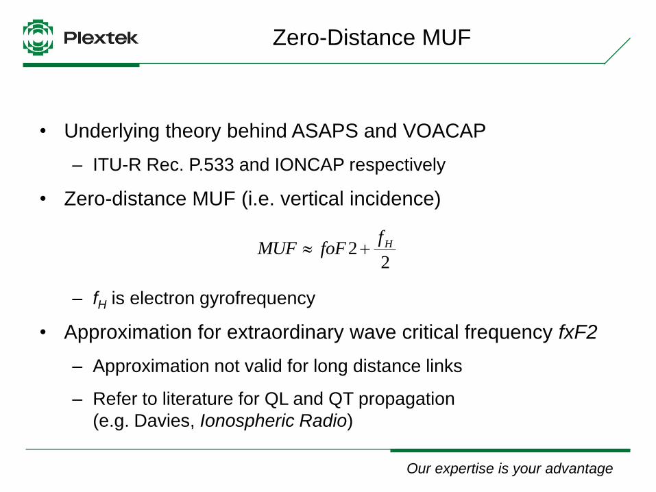
Zero-Distance MUF
• Underlying theory behind ASAPS and VOACAP
– ITU-R Rec. P.533 and IONCAP respectively
• Zero-distance MUF (i.e. vertical incidence)
– fH is electron gyrofrequency
• Approximation for extraordinary wave critical frequency fxF2
– Approximation not valid for long distance links
– Refer to literature for QL and QT propagation
(e.g. Davies, Ionospheric Radio)
22 HffoFMUF

Our expertise is your advantage Company confidential
Chilton Ionosonde Measurements (1)
• Chilton ionosonde
– 51.6°N, 1.3°W
• Data analysed for period 1996-2010
– Manually scaled data (1996-1999)
– Autoscaled data (2000-2010)

Our expertise is your advantage Company confidential
Chilton Ionosonde Measurements (2)
• Autoscaling with ARTIST
– Automatic Real-Time Ionogram Scaler
with True height
• Assumption that ARTIST errors occur
infrequently
– Assumption that errors more likely to
affect upper and lower deciles
– Expert system for validating ionograms
“fails” one-third
McNamara, L. F. (2006), Quality figures and error bars for
Autoscaled Digisonde vertical incidence ionograms,
Radio Sci., 41, RS4011, doi:10.1029/2005RS003440

Our expertise is your advantage Company confidential
Chilton Ionosonde Measurements (3)
• Critical frequency measurements
– foF2
– fxF2 (not a standard ionogram output parameter)
• Spread F Index, fxI
– Maximum F region frequency recorded
– Measure of spread F associated with overhead ionosphere
• When spread F is uncommon
– Median fxI equal to median fxF2
• For this analysis, fxI used in lieu of fxF2
Our expertise is your advantage Company confidential
Chilton Ionosonde Measurements (4)
• Sounding rates varied from 1996 to 2010
– Hourly in 1996
– Every 10 minutes in 2010
• Ionosonde measurements grouped according to timestamp
– Time rounded to nearest hour
– Comparison with ASAPS and VOACAP hourly predictions
• Calculated for each hour
– Median foF2 and median fxI
– Upper and lower decile values (10% and 90%) for foF2 and fxI

Our expertise is your advantage Company confidential
Comparison Methodology
• Measurements compared with predictions
– Median (MUF)
– Upper decile (UD/HPF)
– Lower decile (OWF/FOT)
• Matrix of differences for each hour of each month
– Mean and standard deviation
• Assess
– Diurnal variation
– Month-to-month variation
– Overall performance (1996-2010)
Our expertise is your advantage Company confidential
Comment on Results
• Conclusions from this work specific to Chilton
– More generally the UK
• ASAPS and VOACAP predictions depend on non-identical
global foF2 maps
• Absolute/relative prediction errors depend on geomagnetic
location
Our expertise is your advantage Company confidential
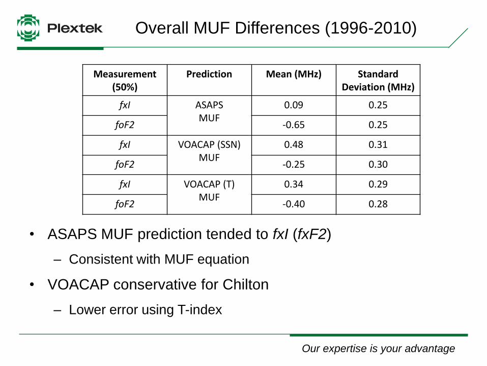
Overall MUF Differences (1996-2010)
• ASAPS MUF prediction tended to fxI (fxF2)
– Consistent with MUF equation
• VOACAP conservative for Chilton
– Lower error using T-index
Measurement (50%)
Prediction Mean (MHz) Standard Deviation (MHz)
fxI ASAPS MUF
0.09 0.25
foF2 -0.65 0.25
fxI VOACAP (SSN) MUF
0.48 0.31
foF2 -0.25 0.30
fxI VOACAP (T) MUF
0.34 0.29
foF2 -0.40 0.28
Our expertise is your advantage Company confidential
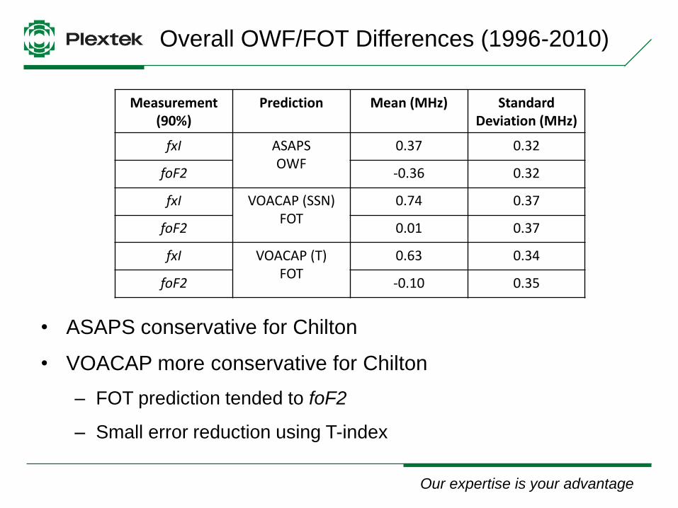
Overall OWF/FOT Differences (1996-2010)
• ASAPS conservative for Chilton
• VOACAP more conservative for Chilton
– FOT prediction tended to foF2
– Small error reduction using T-index
Measurement (90%)
Prediction Mean (MHz) Standard Deviation (MHz)
fxI ASAPS OWF
0.37 0.32
foF2 -0.36 0.32
fxI VOACAP (SSN) FOT
0.74 0.37
foF2 0.01 0.37
fxI VOACAP (T) FOT
0.63 0.34
foF2 -0.10 0.35

Our expertise is your advantage Company confidential
Overall UD/HPF Differences (1996-2010)
• ASAPS UD prediction tended to fxI (fxF2)
– Consistent with MUF equation
• VOACAP conservative for Chilton
– Lower error using T-index (more consistent with MUF equation)
Measurement (10%)
Prediction Mean (MHz) Standard Deviation (MHz)
fxI ASAPS UD
-0.08 0.36
foF2 -0.8 0.36
fxI VOACAP (SSN) HPF
0.36 0.40
foF2 -0.37 0.40
fxI VOACAP (T) HPF
0.18 0.40
foF2 -0.54 0.39
Our expertise is your advantage Company confidential
Results – ALE Frequency Planning
• ALE frequency planning (George Lane)
– Follow diurnal maximum observed frequency (MOF) variation
– Minimum frequency below lowest FOT/OWF
– Maximum frequency close to maximum HPF/UD
• ASAPS might be better than VOACAP for generating UK ALE
frequency scan lists
– Based on overall results
– VOACAP overall results show lower error using monthly T-index
• CAUTION – Still require full link budget analysis

Our expertise is your advantage Company confidential
Results – Monthly Variation (1)
• Difference between
median foF2/fxI and
ASAPS MUF
– Monthly average
– Also T-index
• Cyclical pattern
evident during solar
minimum
• ASAPS MUF tended
to fxI

Our expertise is your advantage Company confidential
Results – Monthly Variation (2)
• Difference between median
foF2/fxI and VOACAP MUF
– Monthly average, SSN and T-index
• Cyclical pattern not evident
• VOACAP using SSN
– Conservative MUF prediction
– Larger errors during solar maximum
• VOACAP using T-index
– Lower errors overall
– Slightly larger during solar minimum

Our expertise is your advantage Company confidential
Results – Monthly Variation (3)
• Difference between median
foF2/fxI and ASAPS and
VOACAP MUF
– Average monthly standard
deviation
• Both show cyclical pattern
– Larger in winter
• Standard deviation generally comparable
– VOACAP standard deviation larger during winter around solar
maximum with SSN
– VOACAP standard deviation lower using T-index

Our expertise is your advantage Company confidential
Results – Monthly Variation (4)
• Cyclical pattern
– Difficulty predicting F2 region ‘winter anomaly’
• VOACAP solar maximum discrepancies
– ASAPS uses monthly T-index
– VOACAP uses SSN (12-month running mean)
– ‘Ersatz’ indices (e.g. T-index) outperform direct indices
(e.g. SSN)
– Sunspot number is only circumstantial index
i.e. no physical basis for direct relationship between sunspot
number and ionospheric response

Our expertise is your advantage Company confidential
Results – Variation over Year 2002 (1)
• Difference between
median fxI and ASAPS
MUF (2002)
• Large positive
differences day and night
during winter and early
spring
• Some months in 2002
show negative
differences during day
and night
Our expertise is your advantage Company confidential
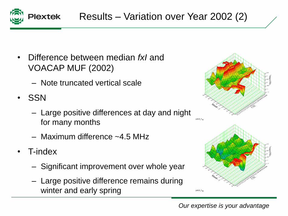
Results – Variation over Year 2002 (2)
• Difference between median fxI and
VOACAP MUF (2002)
– Note truncated vertical scale
• SSN
– Large positive differences at day and night
for many months
– Maximum difference ~4.5 MHz
• T-index
– Significant improvement over whole year
– Large positive difference remains during
winter and early spring

Our expertise is your advantage Company confidential
Results – Variation over Year 2002 (3)
• Measured foF2 and fxI
versus ASAPS MUF
(2002)
• ASAPS MUF prediction
generally consistent with
MUF equation except
above ~12 MHz
Our expertise is your advantage Company confidential
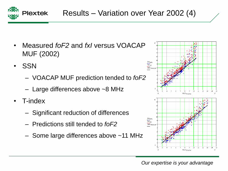
Results – Variation over Year 2002 (4)
• Measured foF2 and fxI versus VOACAP
MUF (2002)
• SSN
– VOACAP MUF prediction tended to foF2
– Large differences above ~8 MHz
• T-index
– Significant reduction of differences
– Predictions still tended to foF2
– Some large differences above ~11 MHz

Our expertise is your advantage Company confidential
Results – Variation over Year 2008 (1)
• Difference between
median fxI and ASAPS
MUF (2008)
• Large positive
differences at night
during autumn and
winter
• Summer months in 2008
show negative
differences during day

Our expertise is your advantage Company confidential
Results – Variation over Year 2008 (2)
• Difference between median fxI and
VOACAP MUF (2008)
• SSN
– Large positive differences at night during
autumn and winter
• T-index
– Large positive differences at night during
autumn and winter
– Degradation in daytime during autumn
and winter

Our expertise is your advantage Company confidential
Results – Variation over Year 2008 (3)
• Measured foF2 and fxI
versus ASAPS MUF
(2008)
• ASAPS MUF prediction
tended to foF2 below
~4 MHz

Our expertise is your advantage Company confidential
Results – Variation over Year 2008 (4)
• Measured foF2 and fxI versus VOACAP
MUF (2008)
• Both SSN and T-index
– VOACAP MUF prediction tended to foF2
below ~4 MHz
• T-index
– Less consistent with MUF equation

Our expertise is your advantage Company confidential
Results – Variation over Year 2008 (5)
• Development of IONCAP
– George Lane
“There was very little data below 4 MHz but there was some for
short paths that did go down to 2 MHz.”
• IONCAP developers modelled a fit to these cases
– Understood to have given good results for NVIS situations
• Presumably, this also applies for REC533 and ASAPS

Our expertise is your advantage Company confidential
Results – Variation over Year 2008 (6)
• Errors in foF2 maps
• Errors due to ionogram autoscaling
– Chilton autoscaled foF2 measurements show positive errors at
LF
• Bamford, R. A., R. Stamper, and L. R. Cander (2008), A comparison
between the hourly autoscaled and manually scaled characteristics
from the Chilton ionosonde from 1996 to 2004, Radio Sci., 43,
RS1001, doi:10.1029/2005RS003401
• Spread F
– High-latitude spread F begins at ~40° geomagnetic latitude
– High-latitude spread F occurs mostly at night

Our expertise is your advantage Company confidential
Results – Solar Indices (1)
• Difference between
median foF2/fxI and
ASAPS MUF against
T-index
• ASAPS MUF generally
within ~10% of fxI
– Except at low or
negative T-index values
• Autoscaling errors at LF?
• Spread F?

Our expertise is your advantage Company confidential
Results – Solar Indices (2)
• Difference between median foF2/fxI
and VOACAP MUF against SSN
(using SSN and T-index)
• SSN
– Large differences for high SSN
(i.e. > ~100)
• T-index
– Reduction in differences for
medium/large SSN (i.e. > ~50)
– Slight increase at low SSN?

Our expertise is your advantage Company confidential
Results – Solar Indices (3)
• Difference between median foF2/fxI
and VOACAP MUF against T-SSN
• SSN
– VOACAP diverges from trends
when T-SSN > ~15
– Identifies periods when Chilton/UK
NVIS basic MUF predictions might
be inaccurate (or pessimistic)
• T-index
– Lower differences for T-SSN > 0
– Slight increase for T-SSN < 0?

Our expertise is your advantage Company confidential
Results – Solar Indices (4)
• VOACAP predictions might be inaccurate (or pessimistic) for
Chilton/UK NVIS basic MUF predictions when T-SSN > ~15
– Assumes real-time access to T-index
• Averaging of effective sunspot number?
• 5-day average “strikes a good balance” (John M. Goodman )
• IPS provide 7-day average
• During solar maximum
– Consider effective sunspot number instead of SSN in VOACAP
• During solar minimum
– Use SSN in VOACAP
Our expertise is your advantage Company confidential
Summary (1)
• Conclusions specific to Chilton (more generally the UK)
• For the period 1996-2010
– ASAPS basic MUF predictions generally agreed with Chilton fxI
measurements
– ASAPS MUF prediction consistent with zero-distance MUF
equation
– VOACAP predictions conservative (particularly around solar
maximum)
– Similar observations for upper decile (10%) predictions
– ASAPS and VOACAP lower decile (90%) predictions
conservative (VOACAP more so)

Our expertise is your advantage Company confidential
Summary (2)
• Below ~4 MHz during winter nights around solar minimum
– ASAPS and VOACAP MUF predictions tended towards foF2
– Contrary to underlying theory
– Autoscaling errors due to nighttime spread F?
• ASAPS errors increased at low or negative T-index values
– Autoscaling errors due to nighttime spread F?
• VOACAP errors
– Greatest at solar maximum using SSN
– Errors might be large when T-SSN exceeds ~15
– Errors reduced when using T-index

Our expertise is your advantage Company confidential
Acknowledgements
• UK Solar System Data Centre, RAL Space
– Allowing the use of Chilton ionosonde data
• George Lane
– Archiving a paper copy of the Nacaskul reference
(now available at the DTIC)