analysis of consumption and emissions of natural gas and
TRANSCRIPT

Equilibre PROJECT
Analysis of consumption and emissions of Natural Gas and Diesel vehicles
Final report
Writers Bernard Schnetzler Fouad Baouche
Proofreaders Anne-Christine Demanny Nour Eddin El Faouzi Pascal Mégevand David Billandon
Versions
From version 1.1 to version 1.4a, corrections have been made to reformulate, add explanations
or additions, and eliminate errors in detail. Version 1.5 contains an additional appendix
providing new results, leaving the conclusions unchanged
Date Version Writers Main modification 13/07/2018 1.1
french B. Schnetzler F. Baouche
01/09/2018 1.2 B. Schnetzler Redactional improvments
12/11/2018 1.3a B. Schnetzler Take into account Mégevand’ s remarks
21/11/2018 1.3b B. Schnetzler English translation of the version 1.3a
26/11/2018 1.4a B. Schnetzler Take into account Billandon’ s remarks
26/11/2018 1.4b B. Schnetzler English translation of the version 1.4a
05/12/2018 1.5a B. Schnetzler Add appendix E
07/12/2018 1.5b B. Schnetzler English translation of the version 1.5a
24/04/2019 1.6a B. Schnetzler Without appendices A, B, C, D
16/05/2019 1.6b B. Schnetzler English translation of the version 1.6a
Last version approved by Nour Eddin El Faouzi, LICIT director, 30/01/2019
© EQUILIBRE – December 2018 – IFSTTAR, 25 Avenue F. Mitterrand – 69675 BRON Cedex.

Analysis of consumption and emissions of Natural Gas and Diesel vehicles 2
PREAMBLE
Unless otherwise noted, the following units and values were used in this report:
diesel fuel consumption: expressed in liters gas consumption: expressed in kilograms CO2 emissions: expressed in kilograms NOx emissions: expressed in grams energy value of diesel fuel: 37.5 MJ / liter energy value of the natural gas: 47.3 MJ / kg diesel density: 0.844 CO2 emissions per liter of diesel: 2.7 kg
C02 emissions per kilogram of gas: 2.75 kg
measured powers (embedded measurements) are indicated powers, which include friction

Analysis of consumption and emissions of Natural Gas and Diesel vehicles 3
TABLE OF CONTENTS PREAMBLE ............................................................................................................................................................................ 2
TABLE OF CONTENTS ...................................................................................................................................................... 3
1. Introduction ..................................................................................................................................................................... 6
1.1. Monitoring of the natural gas composition ....................................................................................... 12
1.2. Monitoring of the gas consumption ..................................................................................................... 12
1.3. Refueling durations..................................................................................................................................... 12
1.4. Natural gas purchasing .............................................................................................................................. 15
2. Project description and project progress ......................................................................................................... 17
2.1. Diaries ..................................................................................................................................................................... 19
2.2. Road categorization .......................................................................................................................................... 20
2.3. Project progress ................................................................................................................................................. 21
2.3.1. Setting up phase ......................................................................................................................................... 21
2.3.2. Results consolidation and detailed analyzes ................................................................................. 23
3. Roads and trips descriptions ................................................................................................................................. 25
3.1. Roads description .............................................................................................................................................. 26
3.1.1. Roads categorization................................................................................................................................ 26
3.1.2. Elevation profile ......................................................................................................................................... 29
3.2. Trips description ................................................................................................................................................ 32
3.2.1. Trip characterization ............................................................................................................................... 34
3.2.2. Mean trip characterization .................................................................................................................... 35
4. Survey of explanatory factors ............................................................................................................................... 37
4.1. Elevation profile ................................................................................................................................................. 38
4.2. Facilities ................................................................................................................................................................. 40
4.2.1. Toll gate ......................................................................................................................................................... 40
4.2.2. Roundabout ................................................................................................................................................. 41
4.3. Traffic ...................................................................................................................................................................... 43
4.3.1. Use of the Annecy ring road .................................................................................................................. 43
4.3.2. Use of the Lyon ring road ....................................................................................................................... 46
4.3.3. Comparing results on both rings ........................................................................................................ 47
4.4. Maneuvers and delivery conditions ........................................................................................................... 48
4.4.1. Results for 44-ton vehicles .................................................................................................................... 49
4.4.2. Results for 19-ton vehicles .................................................................................................................... 53
4.5. The wind ................................................................................................................................................................ 54
4.5.1. Description of wind conditions in Montélimar ............................................................................. 55
Analysis of consumption and emissions of Natural Gas and Diesel vehicles 4
4.5.2. Estimation of wind effects ..................................................................................................................... 56
4.6. Estimation of the engine temperature effects........................................................................................ 58
4.7. Conclusion............................................................................................................................................................. 61
5. Anomalies and dysfunctions .................................................................................................................................. 63
5.1. Power drop ........................................................................................................................................................... 63
5.2. NOx emissions of a diesel vehicle ................................................................................................................ 67
5.3. NOx emissions of natural gas vehicles ....................................................................................................... 68
5.4. Consumption and NOx emissions of a natural gas vehicle – LNG ................................................... 70
5.5. Conclusions .......................................................................................................................................................... 71
6. Results for 44-ton semi-trailers ........................................................................................................................... 72
6.1. Trips characterization...................................................................................................................................... 72
6.2. Vehicles consumption ...................................................................................................................................... 78
6.3. C02 emissions ....................................................................................................................................................... 82
6.4. NOx emissions ...................................................................................................................................................... 85
7. Results for 19-ton rigid trucks .............................................................................................................................. 92
7.1. Trips characterization...................................................................................................................................... 92
7.2. Consumption and CO2 emissions ................................................................................................................. 94
7.3. NOx emissions ...................................................................................................................................................... 97
8. Modeling consumption and emissions ........................................................................................................... 100
8.1. Model for consumption prediction .......................................................................................................... 101
8.2. Model validation and calibration ............................................................................................................. 102
8.3. Estimation of NOx emissions ...................................................................................................................... 106
8.4. Generation of speed cycles.......................................................................................................................... 107
8.4.1. Generation of a simplified urban cycle .......................................................................................... 107
8.4.2. Generation of a complete cycle ......................................................................................................... 109
8.5. Conclusions of the modeling ...................................................................................................................... 112
9. Conclusions ................................................................................................................................................................ 114
9.1. Variability in consumption and emissions ........................................................................................... 114
9.2. Comparative of motorizations ................................................................................................................... 115
9.3. Concentration of NOx emissions in urban areas ................................................................................. 115
Appendix A. Full linear model ................................................................................................................................. 117
Appendix B. Definition of speed extrema ........................................................................................................... 117
Appendix C. Joint distributions and cycle generation algorithm.............................................................. 117
Appendix D. Tables of correlations ....................................................................................................................... 117

Analysis of consumption and emissions of Natural Gas and Diesel vehicles 5
Analysis of consumption and emissions of Natural Gas and Diesel vehicles 6
1. Introduction
The Equilibre project was launched on the initiative of carriers to evaluate comparatively economic and environmental performances of diesel and natural gas vehicles. The objective was the study of vehicles in real operating situation by characterizing the use of the vehicle from the start of the engine at the beginning of the day until the end of the day. This study adopts the point of view of the operator on a vehicle and thus is not limited to the figures announced by a manufacturer.
It is essential to note the difference in point of view between a motorist and a carrier. On the one hand, from a manufacturer's point of view, a vehicle spends energy to accelerate, uplift a load when climbing and overcome friction forces. The explanatory variables are acceleration, instantaneous speed, mass, etc. On the other hand, from the carriers’s point of view this study examines the explanatory factors that they can directly observe or better control. The explanatory variables are then the road, traffic, meteorology, etc.
The in-depth study of actual operating situations on a small fleet distinguishes this project from similar projects, involving either vehicles carrying a large number of sensors but out of real operating conditions1 or with large fleets but with limited information collection2. As much for technical reasons as for cost reasons, an actual operating situation limits the capabilities of on-board measurement and information gathering.
In short, this study is positioned in an intermediate situation, on all levels: we are not interested in the engine of the vehicle or macroeconomic statistics, but in a carrier’s vision of a journey
A real day is made up of multiple loading and unloading operations, journeys punctuated by incidents, empty journeys, stops, refueling, etc. All these points will be discussed, but the study will focus on the route, the traffic, the transported loads and the maneuvers on the customer’s sites. The objective is not to verify an obvious fact - such as a lower average emission of CO2 and NOx for vehicles running on natural gas3 - but to acquire a knowledge of the events punctuating a day and their effects. The objectives of the carriers are multiple: to select the type of vehicle most adapted to some use and to quantify the gains; predict the mean consumption of a new “journey” at the moment of a call for tenders to anticipate its cost (a journey/trip is defined by the identity of the vehicle, a road and a transported load); estimate NOx emissions. The recurrence of the same route over long periods justifies the fact that the focus is on a mean consumption
1 D. C. Quiros et al., “Real-World Emissions from Modern Heavy-Duty Diesel, Natural Gas, and Hybrid Diesel Trucks Operating Along Major California Freight Corridors,” Emiss. Control Sci. Technol., vol. 2, no. 3, pp. 156–172, Jul. 2016. 2 J. Dominguez, F. Mariani, M. Maedge, X. Ribas, and E. Van Gysel, “LNG Blue Corridors position paper,” 2015 3 The CO2 emission rates are 2.7 kg CO2 per liter of diesel and 2.75 kg CO2 per kilogram of natural gas. Compared to the kWh supplied, the emission rates are respectively 0.259 and 0.209 kg / kWh when we take the following energy values: 47.25 MJ for 1 kg of gas and 37.5 MJ for one liter of diesel. When the energy efficiency of gas engines reaches that of diesel engines, the gain in terms of CO2 emissions will therefore be in the order of 20%.

Analysis of consumption and emissions of Natural Gas and Diesel vehicles 7
which is independent of variable traffic conditions, driver identity or seasonal meteorological considerations. This report, based on the project data, goes beyond the objectives of the carriers and the comparison of the different types of motorization. Thus, for spatial planning, it is necessary to know where the emissions are concentrated and what are the impacts of traffic, infrastructures and facilities4.
In this report, in addition to the raw results, we will try to highlight four essential points:
The first is the correction of a cliché considering a road transport dominated by long distances traveled on highway. As will be seen immediately below, this correction is of great importance for pollutant emission estimates.
The second point is the identification of factors that explain consumption and emissions, which are not always the ones that carriers or infrastructure designers and managers think about.
The third point is the importance of the actual operating conditions and the complexity of the description of the use of a vehicle.
The fourth and last point is the great variability of the operating conditions, linked to the multiplicity of explanatory factors, which renders illusory the belief in the existence of typical journey profiles.
If we had to remember only one point it would be that each journey is different.
A number of clichés are associated with road transport. One of them is a reductive vision that considers transport over long distances. It is necessary to correct this image: “78% of the volumes are transported on less than 150 km”5. Long-haul transportation is then a minority compared to distribution journey. Figure 1.1 illustrates the difference in use of the road network observed during the Equilibre project depending on the type of mission. Because of the long-haul transportation, distances traveled on motorways remain majority, but those traveled in urban areas become important thanks to the important part of the distribution: during the Equilibre project, the 9 semi-trailers traveled eight hundred thousand kilometers 61% of which on the motorway and 26% in urban or peri-urban areas. This point is essential when one looks at pollutant emissions and specially in NOx emissions, the health impact of which is more problematic in urban areas than in the countryside; moreover, in urban areas the emission rates are much higher than on the highway. The monitoring of six semi-trailers of 44 tons , with diesel or gas engines, making either distribution or long-haul, thus reveals NOx emissions concentrated in urban areas with percentages varying between 36 and 80%. Thus, we see that the sixth vehicle (see Figure 1.2), although performing long-haul missions with a predominantly motorway use, still emits 51% of NOx in urban areas.
4 Infrastructure refers to the road itself with its general characteristics, such as the existence of access ramps. The facilities are more localized and non-normative features: roundabout, speed bump, toll gate, traffic lights, etc. This report looks at the impact of the particular characteristics of a road on consumption and emissions, be it the general properties of the infrastructure or the particular facilities. NOx emissions can be expressed in g / kWh or g / km; Vehicle studies favors the first formulation; this report, which focuses on the road, favors the second formulation. 5 http://www.fntr.fr/espace-documentaire/chiffres-cles/les-chiffres-blancs-du-trm-francais

Analysis of consumption and emissions of Natural Gas and Diesel vehicles 8
Figure 1.1: Mileage distribution for 44 t tractors – twenty-one months of data
The consumption of a truck depends on a large number of factors: cruising speed (eg. a stable speed on highway), the nature of the road (eg. highway or country road), the density of some facilities (eg. roundabout and traffic light), elevation profile, carried load, traffic intensity, meteorological factors (eg. wind and rainfalls), frequency of stops, frequency of starts cold, fuel quality, etc. These factors are either first-order or second-order, and the ranking is not always the one the carriers think about. Thus the load carried is not a factor of the first order; it will appear that this factor only explains the consumption coupled with other factors, such as the elevation profile.
72%
9%
5% 10%
4%
Long-haul
19%
27%
1%
47%
6%
Distribution
61% 13%
4%
18%
4%
All journeys Class 1 : Motorway Class 2 : Country road Class 3 : Urban expressway Class 4 : Urban crossing Class 5: Dense urban area

Analysis of consumption and emissions of Natural Gas and Diesel vehicles 9
Figure 1.2: NOx emissions distribution – six-month data This figure was made at the beginning of the project (six-month data) on the fleet then available to have an overview of the vehicles use. We will explain later in this report that the definition adopted for urban crossings extends the urban character beyond the perimeter set by the speed limits.
4%
10%
86%
0%
NOx Emissions (%) - Travelled distance: 29878 km
Motorway
Country road
Urban crossing
Dense urban area
Distribution
53%
11%
29%
7%
NOx Emissions (%) - Travelled distance: 65511 km
Long-haul
3%
27%
70%
0%
NOx Emissions (%) - Travelled distance: 25075 km
Distribution
62%
0%
38%
0%
NOx Emissions (%) - Travelled distance: 21815 km
Long-haul
43%
21% 0%
37%
NOx Emissions (%) - Travelled distance: 19073 km
Long-haul
39%
10% 17%
34%
NOx Emissions (%) - Travelled distance: 51869 km
Long-haul

Analysis of consumption and emissions of Natural Gas and Diesel vehicles 10
The third point is the study of vehicles in real operating situation. Unlike laboratory studies, the real-life study never allows a single explanatory factor to be varied, while keeping all other factors constant. Moreover, these factors are rarely independent. Thus road infrastructures and facilities are clearly correlated with the traffic flow, since it is this which justified their creation. Because of this complexity, it is extremely difficult to quantify effects of second-order factors and therefore they have rarely been studied in depth
The fourth and final point concerns the variability of the operating conditions. A carrier performing a mission for a customer performs a recurring trip. For example, once a week for a year, he travels the same 200-kilometer journey with the same load under the same traffic conditions. On the one hand, it can make this trip in a rural area with little urbanization, in plain, with a load of 2 tons and with a free-flow traffic. On the other hand, a second carrier can carry out a similar mission in rural urban areas but crossing many municipalities, in rough terrain, with a 20 tons load and with a dense traffic. Between these two extreme cases, both described as distribution within a rural area, the consumption varies from more than one to two. An overly general definition of a mission category (eg. distribution within rural areas) is therefore insufficient and it is important to characterize a trip more precisely. The other remarkable point is that an annual run of 10,400 kilometers (52 repetitions of 200 kilometers), despite a high mileage, is not statistically significant of all the distribution missions carried out within a rural area.
To conclude, the results obtained on half a dozen vehicles do not claim to provide representative averages of the results that would be obtained on the billion kilometers that would be traveled annually by ten thousand vehicles throughout the French territory. Moreover, at the end of the two years of the Equilibre project, rather than trying to establish averages, the conclusion is that we must be interested in the variances: the first objective of this report is to show the dispersion of the results, in spite of kilometers of tens of thousands of kilometers for each project vehicle. The second objective is a detailed study of journeys. First, we try to explain the consumption of a vehicle on a journey in the order of a few hundred kilometers and whose full characterization is only known after the fact.
Secondly, although we can not predict a priori the consumption of a single journey, which depends on factors unknown to the carrier, such as traffic, weather or special characteristics of the route, however, knowing a general description of the road, its evelation profile and the total laden weight, it will be seen that we can predict the mean consumption for a set of similar journeys (the effects of traffic, weather and special characteristics of the road are then averaged). The development of such a predictive model of consumption will be the subject of the last chapter of the report.
The report plan does not follow the chronology of the project. In addition, since the report is intended for a wide audience, the very technical details, usually presented in intermediate notes during the project, have been omitted. To justify the approach and the conclusions, we nevertheless chose to preserve the outlines of the argument. The report is divided into four main parts:
Analysis of consumption and emissions of Natural Gas and Diesel vehicles 11
the first part consists of two chapters. The first chapter describes the progress of the project. The second describes the characterization of the trips and the principles that guided this characterization.
the second part consists of two chapters. The first chapter presents results highlighting the effects of various explanatory factors of consumption and emissions. The second exposes the difficulties encountered with the vehicles during the experiment.
the third part consists of two chapters. The first chapter presents the results for the 44-ton semi-trailers. The second presents the results for 19-ton rigid trucks.
the fourth and final part presents a model to forecast the consumption and CO2 emissions of a journey. It is also explained why one cannot obtain the same precision in predicting NOx emissions during a trip.
* * *
Due to the novelty of Compressed Natural Gas technology, implementation by carriers on one side and scientific study on the other hand raise particular issues. It was therefore considered necessary to answer certain questions about natural gas technology at the outset. There are many reasons for these questions:
the composition of the gas is not standardized (no international standard) and the engines are highly sensitive to this composition
there is no flowmeter or reliable fuel gauge on the vehicles o it is necessary to calculate the consumption and to validate these
calculation procedures o in the absence of a reliable gauge, the judgmental estimate of consumption
leads to fear running out of fuel the duration of a natural gas refueling is perceived a priori as important
compared to a diesel refueling
For vehicles running on natural gas, the fuel composition is a key factor in any study: "Ethane and propane tend to reduce ignition delays, and increase combustion rates compared to methane, octane ratings are also less favorable than for methane. These three conjugated phenomena increase the risk of clattering (uncontrolled ignition of the mixture under the effect of the cylinder pressure), which is destructive to the engine parts. The engine control reacts by removing the ignition advance (which reduces the efficiency), but beyond a certain level (12 to 15%), it is not manageable”6.
This knowledge of the natural gas composition, dependent on the gas field, is all the more essential as its variability is important. Thus, four studies on gas vehicles announce respective methane levels of 77, 87, 87 and 92%. The problem is that we are far from the satisfaction of such requirements since the synthesis of these studies7 does not indicate if it is molar or mass composition and specifies neither the level of ethane nor the rate of inert gases.
6 Personal communication, Bernard Guiot (CRMT). 7 Barouch Giechaskiel, 2018, “Solid Particle Number Emission Factors of Euro VI Heavy-Duty Vehicles on the Road and in the Laboratory”, Int. J. Environ. Res. Public Health, 15, 304

Analysis of consumption and emissions of Natural Gas and Diesel vehicles 12
1.1. Monitoring of the natural gas composition
As part of the Equilibre project, the composition was monitored on three stations fed by the GRDF distribution network, for a period of two years. This composition comes from the chromatographic analyzes carried out daily. These analyzes indicate the composition by hydrocarbon, from methane CH4 to the heavier hydrocarbons C6H+. We report here only the information considered essential: the Inferior Calorific Power (ICP) as well as the methane, ethane and inert gas levels. Over two years, average ICP is 47.3 MJ / kg; the standard deviation of 0.4 MJ / kg reflects a very stable composition. The composition of the gas is given in Table 1.1. It shows a low content of ethane and other heavy hydrocarbons.
Molar composition: % Mean value (standard-deviation)
Mass composition: % Mean value (standard-deviation)
Methane 92.9 (0.9) 84.5 (1.7) Ethane 4.4 (0.5) 7.5 (0.7) Inerts 2.3 (0.4) 4.6 (0.7) Others 0.4 3.4
Table 1.1: Natural gas composition over three GRDF stations – twenty-four months
Considering the variability of the gas composition, depending on the supplier,
depending on the days and perhaps also on the condition of the supplier tank, the
control of its composition should be imperative.
1.2. Monitoring of the gas consumption
Compressed natural gas vehicles do not have a reliable fuel gauge or flowmeter. This consumption was therefore calculated by the CRMT from exhaust measurements and engine mapping. During a first phase of the project, this calculated consumption was controlled from the billing of gas purchases. This control work proved complex because of data gaps for both the vehicles and the stations. For more details, see a previous report8. It could nevertheless be established that the error in the estimates of consumption should be between 1 and 3%. This small error has no impact on the conclusions of this paper.
1.3. Refueling durations
The completion of refuelings and especially the time spent to perform the operation are issues of concern for carriers. The procedure is complex. The refueling duration is long. The station may be down - defective devices. At the moment, because of the small number of stations, it would be necessary to add the waiting time on some stations as well as the deviation time to join a station.
8 “PROJET Equilibre, Analyse des consommations et émissions des véhicules GNV et Diesel”, Livrable 1, 20 février 2017
Analysis of consumption and emissions of Natural Gas and Diesel vehicles 13
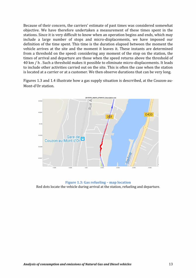
Because of their concern, the carriers' estimate of past times was considered somewhat objective. We have therefore undertaken a measurement of these times spent in the stations. Since it is very difficult to know when an operation begins and ends, which may include a large number of stops and micro-displacements, we have imposed our definition of the time spent. This time is the duration elapsed between the moment the vehicle arrives at the site and the moment it leaves it. These instants are determined from a threshold on the speed: considering any moment of the stop on the station, the times of arrival and departure are those when the speed returns above the threshold of 40 km / h . Such a threshold makes it possible to eliminate micro-displacements. It leads to include other activities carried out on the site. This is often the case when the station is located at a carrier or at a customer. We then observe durations that can be very long.
Figures 1.3 and 1.4 illustrate how a gas supply situation is descrribed, at the Couzon-au-
Mont-d'Or station.
Figure 1.3: Gas refueling – map location Red dots locate the vehicle during arrival at the station, refueling and departure.

Analysis of consumption and emissions of Natural Gas and Diesel vehicles 14
Figure 1.4: Gas refueling – time, speed and emissions profiles
Red dots locate the vehicle during arrival at the station, refueling and departure.
Tables 1.2 and 1.3 show the average duration of gas refueling operations for the main stations used. These tables are respectively associated with 44-ton semi-trailers and 19-ton rigid trucks. The normal duration of a refueling seems to be about twenty minutes. There are thirty-minute durations on the temporary station of Saint-Priest where it is not uncommon for a vehicle to wait for its turn9. The longer durations testify to the existence of another activity. These figures, therefore, refute carriers fears regarding the duration of the refuelings, presumably based on references to exceptional cases10. In summary:
The normal transit time in the station is 20 minutes. (This time would be 30
minutes in case of waiting, but such a figure is related to the exceptional
conditions of experimentation.)
9 Considering the DY491CV, which uses the Couzon-au-Mont-d'Or and Saint-Priest stations, the numbers of "stop & go" during a refueling operation are respectively 5 and 12 for the two stations. Theoretically, beyond one, an additional "stop & go" is interpreted as the advance of the vehicle after the refueling of a vehicle that precedes it. In practice, other facts must be taken into account, such as the possible stopping of the vehicle at the exit of the station before entering the traffic (see figures 1.3 and 1.4). Above all, very low speed displacements on car parks raise measurement problems related, among other things, to GPS drift; this type of particularly complex measure was therefore considered outside the scope of this project 10 The problems observed are rather due to the youth of the technology: low number of stations, involving deviations and waiting times, difficulty of operating refueling devices (drivers must be trained in these operations), and finally defective devices

Analysis of consumption and emissions of Natural Gas and Diesel vehicles 15
Vehicle Station Number of days
Number of transits
Mean duration
DY491CV Couzon-au-Mont-d'Or 405 106 21 mn Villefranche Sur Saône - 10 106 mn (+) Villefranche Sur Saône – Sotradel (*) - 343 46 mn Bourg En Bresse - 2 26 mn Saint-Priest - Provisoire - 68 33 mn EN052KT Couzon-au-Mont-d'Or 63 2 17 mn Villefranche Sur Saône – Sotradel (*) - 2 21 mn Saint-Priest - Provisoire - 37 34 mn DX347RQ Saint-Pierre-en-Faucigny 334 225 21 mn Saint-Pierre-en-Faucigny – Prabel - 51 40 mn Cran-Gevrier - 49 20 mn EL375RS Nimes (**) 202 213 98 mn Cran-Gevrier - 2 34 mn Saint-Priest - Provisoire - 27 32 mn Port-Saint-Louis - 10 93 mn (+)
Table 1.2: Refuelings of 44-ton semi-trailers Refueling is frequently concomitant with other operations. In particular, when a station is located at the carrier or a customer, loading or coupling time is added to refueling time. (*) Station located at the carrier. (**) Station located at the customer. (+) Exceptionnal events.
Vehicle Station Number of
days Number of
transits Mean
duration
EB539DE Couzon-au-Mont-d'Or 400 31 14 mn Villefranche Sur Saône - 85 23 mn Villefranche Sur Saône – Sotradel (*) - 237 23 mn Bourg En Bresse - 1 20 mn Saint-Priest - Provisoire - 135 23 mn EA033ST Saint-Pierre-en-Faucigny 101 113 47 mn Saint-Pierre-en-Faucigny – Prabel - 2 210 mn DY850ZB Saint-Pierre-en-Faucigny 148 65 19 mn Saint-Pierre-en-Faucigny – Prabel (*) - 378 45 mn
Table 1.3: Refuelings of 19-ton rigid trucks (*) Station located at the carrier.
1.4. Natural gas purchasing
Because of the absence of a reliable gauge and a flowmeter, drivers are frightened of running out of fuel. This leads them to multiply the passages in station to make a partial refueling. Table 1.4 therefore shows the mean values of the quantities purchased for each pass and reports the ratio between these quantities and the capacity of the vehicle tank. Passages in an out of order station were excluded from the statistics11. Note that the standard deviation is very high and does not correlate with the average quantity.
11 These failures are generally indicated in the diaries: they give rise to quantities purchased null or very low. Statistical figures with purchased quantities of less than 10 kilograms were excluded

Analysis of consumption and emissions of Natural Gas and Diesel vehicles 16
Vehicle Mean natural gas quantity and standard-deviation
Tank capacity Ratio of the refueling to the
tank capacity
DY491CV 55 kg - 𝜎 = 23 kg 137.5 kg 40 % DX347RQ 82 kg - 𝜎 = 27 kg 137.5 kg 60 %
EB539DE 64 kg - 𝜎 = 22 kg 137.5 kg 46 % DY850ZB 84 kg - 𝜎 = 20 kg 158.1 kg 53 %
Tableau 1.4: Natural gaz purchasing within stations
Figure 1.5: Histograms of refuelings - Vehicle DX347RQ The figure on the left is the distribution over the entire duration of the project. The figure on the right gives the distributions on the first half of the project (in blue) and the second half of the project (in red).
The large variance in the quantities of purchased gas is visible in the distribution observed for one of the vehicles (see Figure 1.5). Given the small quantities purchased during some operations (less than a third of the tank capacity), it seems that some passages in station could be avoided. The question is therefore whether a better estimate of the drivers' consumption and a greater confidence in them did not lead to a disappearance of these operations during the project. We have therefore studied the evolution of quantities purchased over time. For one of the vehicles, the sample was divided into two equal parts. We observe then that the distributions of fuel purchases are practically unchanged and that the average quantities purchased are even decreasing: we go from 85 kg to 78 kg. These results invalidate the hypothesis of any change of the drivers’ behavior. In addition, the disappearance of large volume purchases could be explained by different vehicle operating profiles and changes in refueling stations.

Analysis of consumption and emissions of Natural Gas and Diesel vehicles 17
2. Project description and project progress
During the Equilibre project, just over a dozen vehicles, 44-ton semi-trailers and 19-ton rigid trucks, were equipped. All these vehicles are in EURO VI standard. Because of the hazards of the experiment, the results are only presented for twelve vehicles: 9 semi-trailers and 3 rigid trucks. All rigid trucks have a gas engine, 4 semi-trailers are diesel vehicles, 2 are CNG (Compressed Natural Gas) vehicles, 1 is an LNG (Liquefied Natural Gas) vehicle and 2 are natural gas vehicle with two tanks (CNG+LNG). The vehicles are described in Tables 2.1 and 2.2. These vehicles integrated experimentation on different dates; due to malfunctions, the data series may be incomplete for some vehicles; following the interventions of the manufacturers, some series are not homogeneous.
Cylinder Power Fuel Registrat. Carrier Exploitat. Intervent.
SCANIA 9L 340 hp GNC
DX-347-RQ Mégevand 03-2016 12-2017
07/ 2017
IVECO 8L 330 hp GNL
EA-190-HL Perrenot 03-2016 12-2017
10/2017
IVECO 9L 400 hp GNL+GNC
EL-375-RS Mégevand 05-2017 02-2018
02/2018
SCANIA 9L 340 hp GNC
DY-491-CV Sotradel 03-2016 11-2017
VOLVO 12L 500 hp Gazole DE-477-VE Mégevand 03-2016 12-2017
IVECO 11L 460 hp Gazole DL-928-LJ Perrenot 03-2016 12-2017
05/2017
DAF 13L 460 hp Gazole DS-282-LC Transalliance 03-2016 12-2016
SCANIA 13L 450 hp Gazole EM-644-EF Mégevand 05-2017 12-2017
IVECO 9L 400 hp GNL+GNC
EN-052-KT Sotradel 07-2017 11-2017
03/2018
Table 2.1: 44-ton semi-trailers
It is recalled that the objective of the project is both a study under real operating conditions and a comparison of two types of motorization. It is not a question of comparing the vehicles of the various manufacturers which differ on many points and in particular by the power of the engine, which varies from 330 hp to 500 hp. Finally, as we will see in the report, the usual conditions of these vehicles differ. It is therefore emphasized that generally differences in vehicle characteristics, inaccurate results (<5%) and unobservable variability in the usual conditions only allow general conclusions.

Analysis of consumption and emissions of Natural Gas and Diesel vehicles 18
Cylinder Power Fuel Registration Carrier Exploitation IVECO 8L 330 hp GNC DY-850-ZB Prabel 03-2016: 11-2017 RENAULT 8L 330 hp GNC EB-539-DE Sotradel 04-2016: 09-2017 SCANIA 9L 333 hp GNC EA-033-ST G7 Savoie 10-2017: 02-2018
Table 2.2: 19-ton rigid trucks
The project monitored a dozen vehicles mainly equipped with a NOx sensor, a GPS and an SD card recorder. The probe makes no distinction between different nitrogen oxides. The equipment was installed by the company CRMT.
The data from the NOx sensor, the GPS and the vehicle CAN bus are recorded at a frequency of 5 Hz. The SD cards are retrieved monthly. A non-exhaustive list of the recorded variables is given below:
longitude and latitude date and hour time tag engine speed torque power cruise control activation depressing the brake pedal depressing the accelerator pedal outside temperature oil temperature water temperature fuel flow NOx flow exhaust air flow oxygen flow at the exhaust vehicle speed (tachometer) wheel speed engine fault lights
This data collection is supplemented by diaries, reporting loading and unloading, trailer coupling and decoupling, refueling, and Transport Management System (TMS) and tachograph data that identify drivers and their activities. The important point is that the description of a vehicle journey is enriched with a variable describing at any moment the total laden weight of the vehicle. Through other channels, meteorological information, traffic information and daily gas chromatographic analyzes are retrieved for some refueling stations.
Since gas (CNG) vehicles do not have a reliable fuel gauge or flowmeter, fuel consumption is calculated from exhaust gas composition, gas composition and engine mapping. The CRMT that equipped the vehicles makes a first estimate of the consumption from a hypothetical average composition of the gas; as soon as the information on the composition of the gas in the refueling station is available, a new calculation is carried out by the IFSTTAR according to the composition of the last refueling. This method is very approximate. This estimate of consumption was

Analysis of consumption and emissions of Natural Gas and Diesel vehicles 19
compared with full-to-full measurements: the estimate would underestimate consumption by at most 3% compared to full-to-full measurements, which are themselves approximate because of multiple defects of the information collection. Since this small error has no impact on the conclusions, we will not return to this point.
For some stations, the gas composition is known by daily chromatographic analyzes. Over a period of one year and three stations, we calculate a lower heating value of 47.3 MJ / kg with a standard deviation of 0.36 MJ. This variability of the calorific value is much lower than the uncertainty on the consumption.
Data pre-processing is done by the CRMT: partial qualification of the records, calculation of the gas consumption from the engine speed and motor mapping, calculation of the CO2 emissions, calculation of the indicated torque and calculation of the indicated power. The fact that CO2 emissions are calculated and not measured explains why this paper focuses on the explanation of fuel consumption and NOx emissions.
IFSTTAR is then in charge of all treatments and analyzes. We do not detail the phases of data qualification and data correction.
Particular attention was paid to the control of the diaries filled by the carriers and in particular to the control of the information relating to the transported load. These diaries were corrected throughout the project as errors were revealed by new analyzes.
During the project, on various vehicles, malfunctions were noted, such as abnormal NOx emissions, which required interventions from the manufacturers. The results presented in this paper exclude these periods of dysfunction. The technical details of the interventions made by the manufacturers have rarely been available, but the defects could fall into three categories: design defects (generally corrected after more than one year), failures (quickly corrected by equipment changes) and inappropriate settings of the computer. It is recalled among other facts that a calculator can be set by the manufacturer so as to reduce either consumption or emissions.
2.1. Diaries
Diaries contain three broad categories of information: • loading and unloading operations as well as coupling and decoupling of trailers • refueling operations • a driver identifier; this information was only used to check that certain abnormal
operations were not related to a particular driver
The most important information is that relating to the loading, unloading, coupling and decoupling of trailers. Depending on the vehicle, diaries are available for part or all of the duration of the project. The information, which is manually entered by the carriers' drivers and commercial services, presents numerous errors, which have generally been corrected as the project progresses. Several criteria allow us to suspect a declaration error:
• total laden weight exceeding the maximum authorized weight • no return to empty weight (vehicle + trailer) over a long period • loading orders not followed by unloading

Analysis of consumption and emissions of Natural Gas and Diesel vehicles 20
• lag between observed consumption and consumption predicted by a consumption model
After detection, errors are reported to carriers who correct the diaries. In some cases, several iterations are necessary. In particular, some errors were detected only several months later thanks to the implementation of a model estimating the consumption of the vehicle.
2.2. Road categorization
There is an administrative categorization of roads distributed for example in highway, expressway, national and departmental road. This categorization is based on the identity of the infrastructure manager. However, there is no reason such categorization accounts for the consumption of a vehicle or its emissions of pollutants. There is, however, a correlation between this categorization and consumption. This correlation is linked to the nature of the infrastructures: on the one hand, the most important infrastructures are designed to handle heavy traffic as economically as possible (ensuring a high flow implies a stable traffic speed and then a stable speed yields a low consumption), and, on the other hand, because of their economic importance these large infrastructures are managed either at national level or by specific organizations. As a result, there is a correlation between the administrative nature of the road and consumption.
The example above highlights a fundamental point for this study: the statistical explanation of consumption12 involves looking for correlations between consumption and observable factors. In addition, the prediction of consumption requires that these factors be known in advance.
The correlation between the administrative categorization of roads and consumption remains rather weak. It is therefore necessary to establish a more adequate categorization of roads, based on the criterion of the alleged impact of the road on the consumption. This work was done at the very beginning of the project. It was based on two ideas:
• the categorization is not on an entire road but on road sections; ideally, the length of a section varies between a few hundred meters and a few kilometers.
• urbanization is a major explanatory factor for consumption. There are two reasons for this: traffic increases with the degree of urbanization; urbanization is the source of infrastructure and physical measures (that we will name facilities) such as traffic lights and roundabouts that have a strong impact on consumption. Traffic and facilities are then responsible for slowdowns and accelerations, which are at the origin of high consumption.
This work has led to the definition of five categories of road sections: highway and expressway, country roads, urban expressways, urban crossings and dense urban area. A precise description of these categories will be made in Chapter 3
12 In general, the abbreviated term “the explanation of consumption” is used rather than systematically writing “the explanation of consumption and pollutant emissions”.

Analysis of consumption and emissions of Natural Gas and Diesel vehicles 21
2.3. Project progress
The project took place in two main phases. During a six-month phase we implement the chain of data processing and validate assumptions. The progress of the second phase was conditioned by the events encountered during the first phase. Statistical exploitation of the data and the study of some factors, such as traffic conditions and weather conditions, were initially planned. The variability of the results, however, proved to be greater than expected and it was then necessary, on the one hand, to analyze the routes in more detail and, on the other hand, to increase the mileage to obtain a greater diversity of operating conditions for each vehicle. Observations then revealed malfunctions or anomalies on several vehicles. It was finally necessary to extend the duration of the experiment by nine months, until corrections were made and the operating data confirmed or invalidated the effectiveness of the patches.
2.3.1. Setting up phase
The initial phase was first a period of implementation of the processing chain, secondly a period of control of the values of some variables - gas consumption and traveled distance - and thirdly a period of validation of the hypotheses. Only 44 ton semi-trailers were studied during this phase.
The description of the operations of the data processing chain is not of particular interest. We simply point out the multiplicity of faults and failures that cause the partial loss of data: malfunctions of the GPS or the vehicle bus; gaps in diaries; defective recorders of gas refueling stations; loss of SD cards on which data was recorded; trips outside the mapped area; trips in foreign countries and unmapped private areas; obsolescence of cartography on some areas13; exclusion of the analysis of too short road sections. Some of these data losses may be enough to make all the data of a day unusable. The result is that out of a total of one million kilometers traveled during the entire project, the full statistical exploitation covered only half of the traveled distances. The first data nevertheless yielded preliminary results for six semi-trailers, confirming the relevance of the road categorization but also revealing an important intra-class variability. Some of the results presented in the first report, in February 2017, will be recalled in the next chapter.
The qualification of some data was carried out during these first six months. The estimate of gas consumption was controlled from commercial information provided by gas distributors. The traveled mileage was controlled using different calculation methods: integration of GPS tracks (frequency of 1 Hz), calculation of traveled distances from speeds indicated by the tachometer14 (frequency of 5 Hz) and calculation of distances from cartographic data, after projection of the vehicle positions on a known road. On paths of a few tens of kilometers, the relative lags between the distances calculated by these three methods are less than 1%. The values from the tachometer
13 Mapping was established at the very beginning of the project, while vehicles sometimes borrowed new sections commissioned during the two years of the experiment. 14 The calculation of the traveled distance from the wheel speed depends on a calibration made according to a theoretical tyre diameter. Due to tyre wear, the error can reach 5%. It was not used.

Analysis of consumption and emissions of Natural Gas and Diesel vehicles 22
were finally retained. Finally, the definition of NOx measurement has been clarified. This measure raises two problems:
On-board sensors return a valid measurement only some time after starting the engine; there is thus a strong correlation between a disability flag and a zero speed (see Figure 2.1). The consequence is an indefinite amount of emissions that is not accounted for. On the one hand, these emissions are potentially important, since they are made with a cold engine15; on the other hand, an idling engine emits very little. The answer to the question of estimating emitted and unmeasured quantities is beyond the scope of this report; the only sure thing is that the values given in this report should be increased. Table 2.3 shows, however, the proportion of time for which measures are available. The figures confirm that this absence of valid measurements mainly concerns the vehicle start-up phases during which the speed is zero; the high values for 19-ton vehicles can be explained by distribution missions in urban areas with many stops. This impact of the stops will be explained in the following chapter.
Durations with measurment
Durations without measurment
Zero speed Non-zero speed 44-ton natural gas 93 % 5 % 2 % 44-ton diesel 94 % 5 % 1 % 19-ton natural gas 84 % 10 % 6 %
Table 2.3: NOx measurement durations - twenty-one months
As a rule, this report focuses on explaining the causes of consumption and emissions and ignores data that can not be explained because the vehicle is located on unidentified areas. Unidentified areas are private parks, foreign countries, obsolete mapping, etc. To compensate for this lack, table 2.4 shows the proportions of the NOx quantities emitted according to whether the “roads” are known or not identified. For semi-trailers, there is a high percentage of non-localized emissions; nevertheless we know that most data are issued of maneuvers on private car parks of customers or carriers. For rigid trucks, table table 2.3 indicated a high proportion of unrecorded emissions, because of stoppages (engine off); on the other hand, table 2.4 indicates a very large quantity of localized emissions, because the deliveries of these trucks are frequently made within cities.
Localized emissions Unlocalized emissions
44-ton natural gas 89 % 11 % (*) 44-ton diesel 85 % 15 % (*) 19-ton natural gas 97 % 3 %
Table 2.4: Localization of NOx emissions – twenty-one months of measurment The “localized” attribute does not relate to the GPS position, which is known, but to the characterization of the road or the area where the vehicle is located.
15 These emissions can be measured in the laboratory with a PEMS (Portable Emissions Measurement System), but this is outside the scope of this study conducted under real operating conditions.

Analysis of consumption and emissions of Natural Gas and Diesel vehicles 23
(*) Unlocalized mileages are not very important (in the order of 2 to 3% of the total), but the emission rates per kilometer are very high.
To conclude, given the figures in Tables 2.3 and 2.4, the absence of measurement or the failure to take into account some data do not relate to major amounts. Therefore, it does not call into question the conclusions of the study relating to NOx emissions.
Eventually, this first phase has highlighted the existence of anomalies or malfunctions on some vehicles: engine power deficiency in some circumstances, emissions of pollutants much higher than the expected figures. Therefore, it was necessary to precisely characterize the phenomena to transmit the observations to the manufacturers.
Figure 2.1. Validity of NOx measurment – vehicle day recording
2.3.2. Results consolidation and detailed analyzes
The second phase of the project has three main components. The first component was the consolidation of the statistical results:
• three new six semi-trailers and a 19-ton rigid truck have joined the vehicle fleet • some vehicles have changed mission to achieve greater diversity of use for the
same vehicle
The first part of the project confirmed the relevance of an explanation of consumption by first order factors:
• a specific road categorization by IFSTTAR • the road elevation profile • the total laden weight

Analysis of consumption and emissions of Natural Gas and Diesel vehicles 24
Nevertheless, there would still be significant variability in the results within each road category. The second part was therefore a more in-depth study of various factors explaining this residual variability: facilities, traffic conditions, weather conditions, urban trips, cold starts, vehicle maneuvers, etc.
The third part was the resumption of measurement campaigns after the interventions of the manufacturers on the vehicles with malfunctions and the qualification of the correctives by the Equilibre project.
Finally, the task of developing a predictive model of consumption was spread over the duration of the project.

Analysis of consumption and emissions of Natural Gas and Diesel vehicles 25
3. Roads and trips descriptions
The use of a vehicle can be described at different scales: microscopic, macroscopic and mesoscopic. At the microscopic level, an engineer describes the operation of a motor with a time scale in the order of a tenth of a second and a spatial scale in the order of one meter. The explanatory variables are speed, acceleration, torque, power, etc. At the other extreme, an economist describes the use of a fleet of vehicles travelling hundreds of thousands of kilometers throughout the year. A carrier is interested in an intermediate scale dictated by the use of a vehicle on a day to perform several transport orders. Consumption over a day is then expressed as the sum of consumptions over all sections of traveled road, where ideally a road section is a stretch of a few hundred meters. The time scale, determined by the travel time of a section, is then a few tens of seconds. We are therefore interested in observable explanatory factors with these scales of time and space.
The starting principle is the physical cause: the consumption results from the acceleration phases or more precisely from the depression of the accelerator pedal. The speed instability over a period of a few minutes, which signifies a succession of slowdown and acceleration phases, thus becomes an explanatory factor16 of high consumption. Finally, we establish a second correlation between an unstable speed and a low mean speed: for a truck, which tends to run at a steady speed of 90 km / h, a mean speed of 45 km / h can be interpreted as a vehicle that accelerates from 0 to 90 km / h or decelerates from 90 to 0 km / h. For trucks, which only adopt one cruising speed within a company fleet, this negative correlation between mean speed and consumption is true over the entire speed range. On the other hand, this negative correlation will not exist in the case of private vehicles for which two factors, having opposite consequences on the mean speed, explain a high consumption: an unstable speed, whose consequence is a low mean speed; high cruising speeds (e.g. 130 km / h), the consequence of which is a high mean speed17. We therefore insist on the distinction between a mean speed, whose measurement includes phases of instability, and a cruising speed, which is stable by definition
For a truck, the mean speed is negatively correlated with consumption.
The principle outlined above is use to categorize road sections: a section which contains a stretch where the maximum speed is reduced18 will be a section where consumption will be high.
16 In statistics, an “explanatory” variable of an observation is not a causal factor, but a variable correlated to the observation. 17 Of course, the consumption of a truck is also lower with a cruising speed of 80 km / h than with a cruising speed of 90 km / h, but the question of this variability does not arise because during a trip a vehicle adopts only one cruising speed. It is not the same for a personal car whose cruising speed varies between 90 and 130 km / h during a trip. 18 A section where the maximum speed is reduced (eg. 70 km / h, 50 km / h) is a section where slowdowns and re-accelerations are frequent (winding road, signaling, traffic, interactions with road riparians, etc.).

Analysis of consumption and emissions of Natural Gas and Diesel vehicles 26
As part of the Equilibre project, the categorization of roads was focused on the
main factor limiting speed: urbanization.
3.1. Roads description
The description of the roads was based on data from the French National Geographical Institute19. The 31 departments involved in the project belong to the following regions: Rhône-Alpes, Burgundy, Auvergne, Franche-Comté, Provence-Alpes-Côte-d'Azur and Languedoc-Roussillon. From these data, a graph of 1,800,000 nodes and 3,600,000 arcs describing a network of 400,224 km was made at IFSTTAR.
3.1.1. Roads categorization
The categorization of road sections established by IFSTTAR was based on the identification of observable variables correlated with the degree of urbanization. This approach has led to the definition of five categories of road sections. These categories are thought according to the road use by heavy trucks:
• Motorways: highways and expressways are roads reserved for motor traffic and normally without intersections. Except in exceptional conditions, the traffic flows with a stable speed.
• Urban expressways: an urban expressway is a road reserved for car traffic, which is normally devoid of intersections but with frequent access ramps. According to our definition, this category includes the peripheral expressway and the penetrating motorways at the approach of large cities. On average, the high traffic intensity and many ramps make the speed more unstable than on motorway, which impacts the consumption and especially the emissions. This categorization leaves aside the case of exceptional conditions, such as congestion peaks.
• Dense urban areas: since access to city centers is generally forbidden to trucks, a dense urban area most often refers to the crossings of a few small towns and especially the suburbs of major cities where shopping centers and industrial areas are concentrated . A density criterion was used to define such areas: 1000 inhabitants per km2, which represents 900 municipalities in France out of a total of 36,000.
• Urban crossings: by definition, an urban crossing (villages and very small towns) could be delimited by the speed limit signs. However, this categorization has been extended beyond the speed limit signs because they do not delineate the stretch of road impacted by this urbanization. This extension is justified by the reasons why the approaches of an urban area have an impact on the speed
19 The database BD TOPO ® provided the description of the roads. It describes the entire French road network with metric precision. A road is described by its median axis. In the final phase of the project, the altimetry was recalculated from the RGE ALTI ® bases with a mesh of 5 meters. However, all the results presented in the report depend on the elevation data of the BD TOPO ® database with a mesh of 25 meters.

Analysis of consumption and emissions of Natural Gas and Diesel vehicles 27
instability: the traffic increases; the presence of facilities, such as roundabouts; the vehicle acceleration at the exit of the urban area. Because of these multiple causes, there is no objective rule that allows to say how far beyond a speed sign it is necessary to extend this categorization into “urban crossing”. As part of the Equilibre project, this categorization was based on available data. Thus, in France, the roads are numbered (e.g. N7), but in towns and villages, the streets bear a name (e.g. Adolphe Thiers Street); especially the roads that leave the urban area often have the same name as the street they extend (e.g. Lyon road). This naming criterion of the main roads makes it possible to extend the urban crossing category beyond the strict urban perimeter, but on an arbitrary length. Within some rural area, when the population is concentrated along roads (e.g. valleys) and the villages follow each other closely, this extension of the perimeter of the urban crossing category explains why large mileages are classified in this category.
Country Roads: this category is the default for all sections that do not fall into the previous categories and as such has a high degree of heterogeneity. For example, a road where speed is limited to 80 km / h but located on the outskirts of a large city may have characteristics close to an urban crossing: heavy traffic and facilities (eg. roundabout, speed bump) responsible for high consumption. Such a road has little in common with a road with the same speed limit but located in the countryside.
Categorization rules that are not of major interest and depend on country-specific road and urban characteristics are not detailed. Only the principle is significant: a categorization based on the alleged mean impact on consumption and emissions20. However, it would be possible to improve the description of a road based on an assessment of the density of facilities and other features: roundabouts, speed bumps, traffic lights, intersections, etc.
From the experimental data, the definition of the five categories was validated statistically at the beginning of the project; the results are not presented for the urban expressways because the data were too few. This validation is based on two criteria that explain consumption: average speed, which is negatively correlated with consumption; the number of “stop & go”21. In the following chapters we will verify that we actually obtain consumptions correlated with the established categories. Tables 3.1 and 3.2 report statistics for six 44-ton vehicles during a first phase of the project. Class separability is validated by Wilcoxon Mann-Whitney tests with a significance level of 1% for both mean speed and the number of “stop & go”. Although the Wilcoxon Mann-
20 From an environmental point of view, the categorization of roads according to the urbanization parameter has a second utility: the localization of pollutant emissions by type of zone. As part of the Equilibre project, given the topic of interest of the carriers, only one categorization of the road was used. It would, however, have been preferable to define two descriptive variables of a road section: a variable describing the category according to the consumption point of view; a binary variable describing the urban or rural category of the area, according to the environmental point of view. The delimitation of an emission zone is as problematic as that of a consumption zone: a speed limit sign does not delimit the urbanization perimeter; emissions extend beyond the road sign. 21 After an ad hoc speed filtering procedure (elimination of high frequencies), a “stop & go” is defined by an "inflection point" with a zero speed.

Analysis of consumption and emissions of Natural Gas and Diesel vehicles 28
Whitney tests amply confirm the relevance of categorization, significant variability in the number of “stop & go” remains within a class.
Vehicle 44 t Motorway Country road Urban crossing Dense urban area
DX347RQ 1 15 32 - DY491CV 0 4 31 27 EA190HL 1 5 8 75 DE477VE 1 15 39 71 DL928LJ 1 2 33 - DS282LC 1 7 24 80
Table 3.1: Number of "stop & go" per hundred kilometers – six-month data
Vehicle 44 t Motorway Country road Urban crossing Dense urban area
DX347RQ 80 54 47 - DY491CV 82 61 41 32 EA190HL 79 53 42 28 DE477VE 85 53 44 34 DL928LJ 81 54 42 - DS282LC 81 53 38 29
Table 3.2: Mean speeds (km/h) – six-month data
The relevance of the road categorization was later confirmed on larger samples as well as on 19-ton rigid trucks. Once the relevance of this categorization was demonstrated, it was considered that the “stop & go” criterion was sufficiently representative of a road category. On the one hand, the results obtained for the 19-ton vehicles confirm the relevance of the categorization (see Table 3.3), and, on the other hand, they reveal the differences in exploitation between 44-ton semi-trailers and 19-ton rigid trucks (see Tables 3.1 and 3.3): the number of “stop & go” is twice as high in urban areas for 19-ton vehicles, which distribute in the city center rather than in outskirts. On the other hand, for 44-ton and 19-ton, the number of “stop & go” is similar on motorway and country road, such similarity testifying of identical traffic conditions during transits.
Within dense urban area, the largest number of "stop & go" for 19-ton vehicles has two explanations. The first is that the traffic flow is more irregular in the city center than in an industrial or commercial area of the suburbs of a large city. The second is that typically the distribution profile of a 19-ton vehicle involves many deliveries, and therefore many stops and restarts, while the 44-ton vehicle distribution profile frequently involves a single delivery.
When the number of stops of a vehicle is very high, the total consumption is strongly determined by the number of restarts. Because of too great intra-class variability, the road category (eg. dense urban) is no longer sufficiently explanatory of consumption: for instance, with 204 “stop & go” in dense urban EA033ST presents operating conditions more severe than the DY850ZB with 141 “stop & go”.
Vehicle Motorway Country road Urban crossing Dense urban area
DY850ZB 1 19 71 141 EB539DE 4 9 82 174 EA033ST 1 10 51 204
Table 3.3: Number of “stop & go" per hundred kilometers

Analysis of consumption and emissions of Natural Gas and Diesel vehicles 29
To summarize, we draw three conclusions from a categorization of road sections according to the use made of them by heavy trucks:
1. The categorization of roads is a relevant explanatory factor.
2. Urbanization is a major factor of the speed instability and consequently of
consumption.
3. Significant variability remains within a category, particularly in urban
areas. where the type of mission of the vehicle is a major explanatory
factor.
3.1.2. Elevation profile
The elevation profile determines consumption in an extremely complex manner. To account for an average effect of this profile, we therefore had to make many approximations, which will be completely justified only by the final result. Our goal is not to explain the physical behavior of vehicles, but to provide statistical findings.
The elevation difference is a major factor of the consumption, which is the expenditure of energy to raise a load. Figure 3.1 is an illustrative example of this statement: for a vehicle with a total laden weight of 30 tons and traveling at 90 km / h, a slope of 1% increases the average fuel consumption by 45%22.
This preliminary observation makes it possible to formulate a first warning: although a slope of 1% is considered as low and therefore is associated with lowland trips, the impact on consumption is very high. On a path whose total slope is zero, it is the compensation phenomenon when the slope is negative which limits this extra consumption. However this compensation phase is not perfect and is very variable ; the first kilometers of the path of Figure 3.1 illustrate this phenomenon of partial compensation.
As part of the Equilibre project, for the explanation of consumption, a simple approach compatible with the available data was retained. Each road section, whose slope is assumed to be of constant sign, is characterized by an elevation difference, which is either positive or negative. The description of a route is then completed by two variables: the cumulative positive elevation across all sections; the cumulative negative elevations across all sections23. In practice, as most trips involve a return to the starting
22 This result does not extrapolate to higher slopes, because the overconsumption does not depend on the load elevation only. The slope increase, which leads to a speed reduction, as well as the capping of the engine power mean that the driving conditions are not identical. 23 The value of the cumulation depends on the description scale of the sections: the cumulation will be lower for a cartography on a smaller scale with a higher smoothing of the altimetric profile.

Analysis of consumption and emissions of Natural Gas and Diesel vehicles 30
point (∆𝑧+ = ∆𝑧−), a path may be described macroscopically by the accumulation of positive elevations24.
Figure 3.1: Consumption according to the elevation profile and the speed In the bottom figure, the first peak of average consumption (in red) is associated with the elevation peak in the top figure, with an ascending slope of 1%. It is followed by a negative peak of consumption in the subsequent descent phase. Finally, the average consumption (kg / 100 km) between kilometers 2 and 6 is barely higher than consumption over the first two kilometers.
During the project, we were confronted with very macroscopic approaches claiming to characterize the roads by the slopes encountered: trips in plains, in rough terrain and in mountains. This characterization, which is carried out on the basis of the maximum slopes of the roads, is far too poor compared to that based on the accumulation of elevations25. However, it raises the question of the effect of the slope.
This question of the effect of the slope is illustrated by the interpretation of Figure 3.2. produced from the highway trips of all diesel vehicles. The sections of all trips were
24 This indicator accounts for the impact of ascents on the consumption increase, with a slightly smaller consumption reduction during descents (assuming a zero total elevation difference). If a trip had only ascents, the kilometer consumption would obviously be much higher. 25 Remember that the elevation difference is the integral of the slope as a function of the traveled distance.

Analysis of consumption and emissions of Natural Gas and Diesel vehicles 31
divided into three classes according to the slope value. The figure gives the mean consumption according to the slopes encountered; the total elevation difference is zero for each class. We see a very high consumption on sections whose slopes are between 2 and 5%. This result is explained firstly by the fact that, in absolute value, the mean slopes are respectively 0.5, 1.5 and 3.5% for the three classes and that the accumulations of the positive elevations are in the same ratio. However, between the first two classes of slopes, the consumption difference is 1.3 liters for a difference of cumulative positive elevation equal to 1%, while between the last two classes of slopes, the consumption difference is 10.9 liters for a difference in cumulative positive elevation equal to 2%. This very high consumption difference per unit of elevation difference means that the slope itself is an explanatory factor.
To sum up, the previous paragraph, based on the observations in Figure 3.2, shows that the added consumption is not the same depending on whether one goes up a thousand meters with a slope of 1% or 5%. For steep slopes (> 2%), consumption increases sharply. In theory, the cumulative positive elevation is not enough to explain overconsumption; however, in practice, we will see in Chapter 8 that the average consumption is predicted with a good precision taking into account only the cumulative positive elevation26. This observation shows simply that, on a full path, the impact of the slope is weak.
Figure 3.2: Mileage consumption depending on the slope Each bar is produced by summing consumptions and mileages on highway sections whose slope is within the specified intervals. For each bar, the total elevation difference over all sections is zero. The distances covered are respectively 51,000, 17,000 and 18,000 kilometers Note that on highway, where the sections are of great length, the average slopes are accurate.This is not the case in urban areas where sections are very short
26 We obtained such results with vehicles which made trips in Savoie (A41 motorway) and in Massif Central (A89 motorway) with a significant mileage (21% of the total) achieved with slopes included between 2 and 5%.
25,2 26,5
37,4
0,0
5,0
10,0
15,0
20,0
25,0
30,0
35,0
40,0
[-1%, 1%] [-2%, -1%] et [1%, 2%] [-5%, -2%] et [2%, 5%]
Co
nsu
mp
tio
n (
l/1
00
km)
Slopes
Mean consumption - Diesel vehicles - Highway trips

Analysis of consumption and emissions of Natural Gas and Diesel vehicles 32
Different cases of flat section show that neither the elevation difference nor the slope are sufficient to characterize a section:
• a flat section, preceded and followed by flat sections • a flat section, preceded by a descent, where the vehicle continues its momentum • a flat section, followed by a climb, where the vehicle accelerates
Mean consumptions vary widely for these three cases of flat sections. They depend on the slopes of the upstream and downstream sections but also on the length of the sections. Without going further into detail, it appears that the elevation profile conditions consumption in a very complex manner and that the slope of the section is only one explanatory variable among others. For this reason, we chose to limit ourselves to the most explanatory factor (the elevation difference) and then to produce a mean estimate of the consumption.
For the elevation difference, as for all the other explanatory factors studied during the Equilibre project, we do not claim to explain the consumption on a specific road section but to give a mean value averaged over several hundred kilometers in very different situations.
At the end of this preliminary study, it appears that the elevation profile conditions consumption in a very complex way. Nevertheless, we can explain mean consumption only from the expression of elevation differences. Two major conclusions are needed:
1. The accumulation of positive elevations is a relevant macroscopic variable
to a trip description.
2. A typology of roads according to the type of terrain (plain, hilly terrain and
mountain) is too weak a description.
3.2. Trips description
The vehicle position is known from the coordinates returned by the GPS. A vehicle is then located on an edge of the network, which carries information on the road category and the elevation difference. At the end of this localization, the initial description of the trip of a vehicle is enriched with two variables indicating the edge identity and the road category. From this enriched description, later, it will be possible to segment the vehicle trip in homogeneous sections. A homogeneous section is the concatenation of edges with identical category and same sign of the elevation difference - the total laden weight of the vehicle must also be unchanged. The elevation difference of a section is the cumulative elevation difference of edges. The complete trip is a sequence of homogeneous sections (see Figure 3.3).

Analysis of consumption and emissions of Natural Gas and Diesel vehicles 33
Figure 3.3: Trip segmentation
The success rate of the localization on a road of the network is in the order of 98%, with an average distance of 3.5 meters between the coordinates of the vehicle and the projection point on the network. The 2% non-projectable points (considered too far away) generally correspond to the presence of the vehicle on private parts, outside the mapped network. There are some other causes of location failure: obsolescence of map data; a route beyond the boundaries of the mapped area (Switzerland and Italy); abnormal use of the road network (counter-directional use when roadworks involves traffic diversion); a malfunction of the GPS.
Many points not projected on the network correspond to deliveries on private parts. As the movements associated with deliveries are made at low speed the traveled mileage on a non-mapped zone is proportionally smaller than the elapsed time27. On the other hand, the consumption and emissions of a 44-ton tractor during such maneuvering phases are extremely high (see Figure 3.4). Therefore, we cannot ignore these 2% of non-localized points on the network.
27 The number of points is proportional to the elapsed time with the engine on. In this type of situation (low mileage on parks), it is frequently proposed to replace the kilometer consumption by the hourly consumption. This proposal does not seem sensible, because besides the fact that it introduces a new criterion difficult to compare to the previous one, the definition and the measurement of the duration are problematic: the spent time with an engine on, the spent time with a nonzero speed, the time spent on the site?

Analysis of consumption and emissions of Natural Gas and Diesel vehicles 34
Figure 3.4: NOx emissions during a trip – NGV Maneuvers are very localized, in space, with very high emission rates.
3.2.1. Trip characterization
From the consumption point of view, the vehicle trip can be divided into two main categories of activity: the displacement phases and the maneuvering phases. The maneuvers are related to the loading and unloading operations as well as to the coupling and decoupling operations of the trailers. Resting stops, refueling and customs clearance are marginal activities.
Although most of the points not located on the network correspond to maneuvering phases, there is no bijection between these two sets: some of the non-projected points do not correspond to maneuvers; many maneuvers are localized rightly or wrongly on the mapped network. There are two cases of maneuver localization on the network: a maneuver may actually be performed on the mapped part of the network; given the margin error28 tolerated in the projection operations, a vehicle located in an area very close to the mapped network may be localized on the mapped network.
In the case of the Equilibre project, we discussed the description of a trip with two different angles of approach: the description of the displacement phases; the description of the maneuvers. The displacement phase was described from the points projected on the network; we left out the remaining 2%. The temporal and spatial location of the maneuvering activities was carried out from diaries data, indicating the loading, unloading, coupling and decoupling operations; another approach is possible because, once the description of the trip has been produced, the breaks in the load are sufficient to locate the maneuvering phases. It should be noted that, due to false projections on the
28 On the one hand, the precision of the GPS within the countryside and the precision of the cartography allow a small margin of error (≤ 10 meters), but on the other hand the inaccuracy of the GPS within a dense urban area (high buildings) imposes a high margin of error (≥ 15 meters). It is this last value that has been retained.

Analysis of consumption and emissions of Natural Gas and Diesel vehicles 35
network, the displacement phases may include maneuvering activities (first case), while maneuvering activities include a displacement phase corresponding to the entry and exit of the site (second case). In some exceptional situations, because the consumption is extremely high during maneuvers, the first case is problematic; the second case is not a problem because the contributions of the entry and the exit to the site are usually marginal.
Due to very high fuel consumption and emissions, maneuvering activities, which depend on vehicle missions, can contribute significantly to the overall result despite low mileage. The study will show that the difference is visible between a vehicle that carries out long-haul transport and performs 1 maneuver per 150 kilometers and a vehicle that distributes and performs 1 maneuver per 30 or 60 kilometers. Finally, when the frequency of the maneuvers becomes even higher and the loads are very heavy, the maneuvers become a major explanatory factor.
The problem of the cost of maneuvers is found again with rigid trucks. On the one hand, stops can be three to four times more frequent than for tractors. On the other hand, the maneuvers of a rigid truck are simpler than docking a semi-trailer and therefore they are less expensive. Eventually, for these vehicles, whose deliveries can be made with roadside stops, it is finally difficult to dissociate the deliveries from the displacement phase.
3.2.2. Mean trip characterization
A trip is described by a succession of section crossings. Each element of the sequence is described by the road category, its length, the elevation difference and the total laden weight. The vehicle identity is a common variable for all elements of the sequence. Such a description does not take into account:
the driver’s identity the traffic conditions prevailing on the date the trip is made the weather conditions prevailing on the date the trip is made
o wind o temperature o rainfall
facilities (eg. roundabout, traffic lights, etc.) of the road sections
The selected variables – road category, elevation profile and total laden weight – have known values before a trip is made. It is therefore possible to base a predictive model of consumption on the basis of these variables. It is a mean prediction, independent of the date of the trip: such a mean prediction interests a carrier whose vehicle can make the same trip once a week for one year.
The statistical representativeness of spatial or temporal means is questionable in some cases. Whether a trip is made 1 or 52 times a year does not change the representativeness of the sample of traveled sections. If some of these sections have very particular characteristics, the spatial mean will not be representative of all the sections of the same category. If consumption is conditioned by recurring traffic

Analysis of consumption and emissions of Natural Gas and Diesel vehicles 36
conditions, and the trip is made at the same times throughout the year, the time average will not be representative of all traffic conditions. However, this reproduction of the same routes at the same times is the rule in real operating situation. This led us to ask carriers to assign their vehicles to different missions during the second part of the project.

Analysis of consumption and emissions of Natural Gas and Diesel vehicles 37
4. Survey of explanatory factors
The objective of this chapter is to present the various factors explaining consumption and emissions by linking them to the original cause: consumption and emissions are directly related to the depression of the accelerator pedal or to the power (more exactly it depends on 𝑊 = 𝑃 × ∆𝑡). The case of consumption is trivial: the consumption is directly proportional to the power developed. The case of NOx emissions is more complex because, on the one hand, the production of NOx is directly related to the consumption, ie. to the “power”, and on the other hand, the elimination of NOx is related to the effectiveness of the pollution control system. However, this efficiency is reduced during the phases of strong acceleration. Figure 4.1 shows two successive cases. The first phase is an acceleration phase, where the four power peaks are associated with the gear ratio changes. Emissions are high. During the second phase, the speed is stable. A much lower ratio is observed between the emissions and the “power”.
Figure 4.1: NOx flow depending on the power - DIESEL
The previous observation is fundamental for three reasons:
in terms of physics, the consumption and emissions (emission = production - elimination) of NOx by a diesel vehicle are not always explicable by the same variables
when consumption can be explained with a property 𝑓(𝑥, 𝑡) of the road or easily observable traffic, transient-dependent NOx emissions will generally depend on the time derivative 𝜕𝑓/𝜕𝑡 or the spatial derivative 𝜕𝑓/𝜕𝑥 which are more difficult to observe. A reliable and accurate prediction of NOx emissions is therefore more difficult
the rules for explaining NOx emissions will depend, among other factors, on the specific pollution control system of each vehicle; because there are several remediation technologies, we have not tried to establish precisely the links between the power developed and the emissions

Analysis of consumption and emissions of Natural Gas and Diesel vehicles 38
It has been explained in the previous chapter that the speed instability can be seen as an explanatory variable of consumption and emissions, but it is not a variable that can be observed on a map. The objective is therefore to consider only observable or searchable “geographical” factors that explain consumption. This study is extended to all explanatory factors that can be known in advance, which explains the heterogeneity of the list below:
the elevation profile facilities traffic maneuvers or delivery conditions the wind cold starts
We do not speak again of the road categorization which has been studied at length in the preceding chapter.
4.1. Elevation profile
The effect of the elevation profile on consumption was studied in the previous chapter. Now, we are interested in the effects on NOx emissions: Figure 4.2 uses the same data as used in Figure 3.1 (see § 3.1.2) for a diesel vehicle. Considering the first five kilometers, the peak of the mean consumption is associated with the peak of the elevation profile, with a road slope of 1%. The increase in consumption is 45%. This consumption peak is associated with a peak of NOx emissions for which the increase is 215%. The second peak of consumption, with an increase of 74%, is linked to a re-acceleration following a fall in speed. It is associated with it a peak of NOx emissions for which the increase is 980%. The relationship between the emission rate and the consumption is therefore strongly non-linear and therefore the definition of a fixed emission rate as a function of the power (g / kWh) is meaningless. In concrete terms, the important result is that constant moderate consumption has little effect on NOx emissions. This result will be confirmed on more aggregated data when studying the effects of a regular moderate wind.

Analysis of consumption and emissions of Natural Gas and Diesel vehicles 39
Figure 4.2: Consumption and NOx emissions - DIESEL
The previous conclusions also apply to a gas vehicle traveling the same route (see Figure 4.3). The relationship between the emission rate and consumption is highly non-linear
Figure 4.3: Consumption and NOx emissions - NGV
Engine studies measure emissions in g / kWh to be independent of certain operating conditions, such as elevation difference and total laden weight. The relevance of this measure is called into question by the fact that the volume of NOx emissions depends as

Analysis of consumption and emissions of Natural Gas and Diesel vehicles 40
much on the way the power is requested (continuous power or sudden variations in power) as on the mean power:
1. Low constant acceleration has little effect on NOx emissions
2. The relationship between power and NOx emissions is strongly non-linear
4.2. Facilities
The objective of this part is the study of the effects of two facilities: a toll gate (with electronic toll collection) and a roundabout. However, in real operating conditions, it is difficult to completely isolate a factor - the electronic toll or roundabout - and to define a reference situation. Therefore we take into account the other factors present on the trip: the elevation profile, roadworks and stops imposed by the regulatory rest of a driver.
4.2.1. Toll gate
Figures 4.2 and 4.3 are respectively associated with a diesel vehicle and a natural gas vehicle that take the same route. The drop speed to the value of 11 km / h observed at the tenth kilometer corresponds to the crossing of the electronic toll system at Crolles on the A41 motorway. It associated with it a strong peak of emissions. The other two speed drops observed in Figure 4.3 are associated with lane changes imposed by counter-directional use of the highway (see Figure 4.4). The repeated nature of such changes for several days suggests that a roadwork is the cause.
Figure 4.4: Counter-directional use of the highway A41

Analysis of consumption and emissions of Natural Gas and Diesel vehicles 41
In view of these preliminary results, it appears that a toll gate (with electronic toll collection) or roadworks, causing slowdowns, have a major impact on NOx emissions. A quantitative analysis was therefore undertaken on the basis of repeated transits on the same route by two diesel vehicles. During twenty-one months, the first made 30 transits and the second 10 transits. Not only was roadwork observed on some of the days considered, but some drivers also had their regulatory rest on the area of Saint-Nazaire-les-Eymes, located just before the toll. Such a rest implies a restart and therefore has a cost in terms of NOx emissions. In the results, we have distinguished the trips including or not the toll, roadwork and stops. The results are reported in Tables 4.1 and 4.2. On average, compared to an ideal trip, the impact of tolls and other hazards on consumption is moderate: a difference of 4%. On the other hand, compared to an ideal route, the impact of tolls and other hazards on NOx emissions is significant: a difference of at least 40%. It should be noted that the relative impact of the toll decreases with the length of the trip, while this relative impact is independent of the trip length for other hazards (roadwork, regulatory stop) whose frequencies are proportional to the traveled distance.
Trip without the toll section
Normal full trip
Full trip with
roadwork
Full trip with rest
Average of all trips
DE477VE 27 29 31 29 29 EM644EF 26 27 - 29 27
Table 4.1: Consumption (l/100 km)
Trip without the toll section
Normal full trip Full trip with
roadwork
Full trip with rest
Average of all trips
DE477VE 15 18 38 29 21 EM644EF 15 19 - 63 23
Table 4.2: NOx emissions (g/100 km)
4.2.2. Roundabout
This paragraph is purely illustrative. It shows the impact of facilities on consumption and pollutant emissions. It confirms what was observed at the Crolles electronic toll gate on the A41 motorway.
The fact that during a trip any slowdown is followed by a re-acceleration, accompanied by peak consumption and emissions, is obvious. What the results of the Equilibre project show is that the mean consumption and emissions are determined by the frequency of these re-acceleration phases during which the consumption is frequently twice that observed when the speed is stabilized.
Figures 4.5 and 4.6 refer to a 5-kilometer trip with a mean negative slope of 0.6%. The trip was made in Meyzieu, in the suburbs of Lyon. It was carried out around 9 pm, therefore in the absence of traffic. The vehicle is a LNG tractor with a total laden weight of 25 tons. Although the road, with a speed limit of 80 km / h, is not classified as being

Analysis of consumption and emissions of Natural Gas and Diesel vehicles 42
located in an urban area, its facilities make it similar to an urban crossing: on a 5-kilometer route, there are three roundabouts causing slowdowns dropping speed to around 25 km / h. The first two re-acceleration phases extend over a length of approximately 0.5 kilometers; inside each of these phases, each peak corresponds to a gear change.
Figure 4.5: Road with a speed limit of 80 km/h within Meyzieu (Lyon suburb)
Figure 4.6: Trip characterization within Meyzieu (Lyon suburb)
Examination of the re-acceleration phases, which extend over 500 meters, highlights the fact that there is little difference between a complete stop and a slowdown to the speed of 10 or 20 km / h; in both cases, the vehicle will accelerate to 80 km / h.

Analysis of consumption and emissions of Natural Gas and Diesel vehicles 43
The characterization of a route can be done either a priori according to geographical information or a posteriori from displacement data. In the first case, in addition to its categorization, the road could be characterized by the density of facilities: roundabouts, speed bumps, intersections, traffic lights, etc. In the second case, in addition to its categorization, we used the mean speed29 and the number of “stop & go”. However, as we have just seen, a slowdown has about the same effect as a complete stop. Ideally, the characterization should therefore take into account these severe slowdowns; such a work, which involves in-depth research, has not been undertaken during the course of the project, but we present some theoretical considerations. To calculate such an indicator and even to estimate the real impact of a “stop & go”, one should not consider the stop or the slowdown, which present no cost, but the phases of re-acceleration with a long duration. Thus, the re-acceleration phases could be accounted for from a low speed (e.g. 10 or 20 km / h) to a high speed (e.g. 60 or 80 km / h). However, such a count has two shortcomings: it depends on arbitrary thresholds; it ignores split acceleration phases during which the vehicle accelerates, slows down a bit, then reaccelerates. Finally, a good indicator of the speed instability would be the ratio of the cumulative positive speed difference 𝛥𝑣 over the traveled distance.
4.3. Traffic
The impact of the mean traffic, mixing off-peak hours and peak hours, is taken into account in the definition of road categories. In this section, we seek to go beyond this estimate of the mean effects; in concrete terms, the objective is an estimate of the effects of heavy traffic on consumption and emissions.
We have chosen to study the effects of traffic on urban peripherals where the impact of congestion is important and where it is therefore easier to measure. That being said, not all peripheral boulevards are multi-lane highways with relatively homogeneous characteristics, as can be seen in Lyon or Paris. In contrast, by-passes of smaller cities have sections with different characteristics. Rather than seeking out the criteria for segmenting such peripheral boulevards into homogeneous sections, which is a complex task, the vehicle trip was arbitrarily decomposed into sections of a length in the order of 2 kilometers; the minimum length of a section is 1 km. For a given vehicle, twenty-one months of operation then provide several hundred observations. Two sites were selected: the Laurent Bonnevay ring road around Lyon; the departmental D3508 around Annecy. On each of these sites, the effect of the traffic was studied for a diesel vehicle and a natural gas vehicle. For each vehicle, consumption and NOx emissions are reported based on the speed of the vehicle on the section - the vehicle acting as a Floating Car, this speed is supposed to be an indicator of congestion.
4.3.1. Use of the Annecy ring road
The ring road of Annecy is defined by the departmental D3508 which bypasses Annecy. It is used by the vehicles of the company Megevand, whose head office is located in
29 It should be noted that the speed variance is irrelevant because it ignores the temporality of the distribution: there is no difference in variance between the series 00001111 and 01010101.

Analysis of consumption and emissions of Natural Gas and Diesel vehicles 44
Sillingy in the suburbs of Annecy. The study is not intended to characterize the ring but the use that is made by some vehicles.
Because the D3508 (according to the administrative classification, it should be a secondary road) does not have the characteristics of an expressway, automatic categorization does not put this road in the category of urban expressways. It does, however, have certain characteristics, such as traffic lane separator, the presence of interchanges and access ramps in place of intersections. It differs in other points: we have a single lane in each direction for the bypass of Annecy, instead of a minimum of two lanes on expressways; speed limits vary between 50 and 80 km / h instead of 70 to 80 km / h on an express lane.
Figure 4.7: Annecy’s ring
Statistical informations on the trips are reported in Table 4.3. Consumption and emissions are shown in Figure 4.8 for a diesel vehicle and a natural gas vehicle. These data result from twenty-one months of measurements.
Mileage (km)
Mean speed (km/h)
Consumption (…/100km)
NOx emissions (g/100 km)
DE477VE (diesel) 2521 52.9 31.2 l 160.3 DX347RQ (gas) 5293 54.5 27.6 kg 33.2
Table 4.3: Use of the Annecy’s ring
Without detailing the interpretation of Figure 4.8, there are clearly at least two clusters that can be associated with a free-flow phase for speeds above 60 km / h and a congested phase for speeds below 40 km / h. For the natural gas vehicle, the negative

Analysis of consumption and emissions of Natural Gas and Diesel vehicles 45
correlations between mean speed on one side and consumption and emissions on the other side are clearly visible.
In the present case, the two vehicles do not use the same sections of the D3508 with the same frequencies, traffic conditions and total laden weights - the CNG vehicle replaced the diesel vehicle in operation. Same mean speeds for both vehicles and similar consumptions are observed (see Table 4.3); since the average speed and the consumption are indicators of the mean state of the traffic, we consider that the use of the ring is carried out under similar conditions for the gas vehicle and for the diesel vehicle. Given this similarity in operating conditions, the important result is that the NOx emission rate is five times lower for the gas vehicle (see Table 4.3 and Figure 4.9)
Figure 4.8: Consumption and emissions - DIESEL (up) et NGV (down) Note that the NOx scales differ by a factor of 10.

Analysis of consumption and emissions of Natural Gas and Diesel vehicles 46
Figure 4.9: Comparative of NOx emissions – DIESEL and NGV
4.3.2. Use of the Lyon ring road
The Lyon ring road, which is the departmental D383, is categorized as an expressway. It is used by Perrenot’s vehicles that make trips between East Lyon and Clermont-Ferrand. The study is not intended to characterize the ring but the use that is made by some vehicles.
Statistical information on the trips is reported in Table 4.4. Consumption and emissions are shown in Figure 4.10 for a diesel vehicle and a natural gas vehicle. These data result from twenty-one months of measurements.
Mileage (km)
Mean speed (km/h)
Consumption (…/100km)
NOx emissions (g/100 km)
DL928LJ (diesel) 490 71.0 27.4 l 20.0 EA190HL (gaz) 9496 71.7 25.4 kg 18.1
Table 4.4: Use of the Lyon’s ring
Without detailing the interpretation of Figure 4.10, it is clear that vehicles use the ring almost exclusively during periods of free-flow traffic. This conclusion is confirmed by high mean speeds for both vehicles, reported in Table 4.4.
The comparison of the results for the diesel vehicle and the natural gas vehicle must be done carefully because the two vehicles do not use the same sections of the D383 with the same frequencies, the same traffic conditions and the same total laden weight. However, the same mean speed for both vehicles and similar consumptions are observed (see Table 4.4); since the mean speed and the consumption are indicators of the mean state of the traffic, we consider that the use of the peripheral of Lyon is carried out under similar conditions for the natural gas vehicle and for the diesel vehicle.

Analysis of consumption and emissions of Natural Gas and Diesel vehicles 47
Considering a traffic almost always free-flow, we then observe an almost identical NOx emission rate for the two vehicles.
Figure 4.10: Consumption and emissions - DIESEL (top) et NGV (down) The natural gas vehicle has traveled a mileage twenty times higher than the diesel vehicle; this explains the higher number of points.
4.3.3. Comparing results on both rings
The differences observed between the observations made on the Annecy and Lyon rings come under different operating conditions. In the second case, there are very few observations in congestion not because the Lyon ring road is not very congested, but because the transport planning has been established in such a way as to allow the vehicles to avoid congestion peaks. On the other hand, on the Annecy site the trucks can not avoid congestion peaks, because in this case the carrier's head office is in the suburbs of Annecy and some of these trips are departures and returns to the depot. In a more general way, the times of transit of the vehicles are constrained by the requests of the customers. This observation raises two problems:
the mean consumption and emissions values are meaningless when there is a mix of two distributions (a distribution for free-flow traffic and a distribution for congested traffic).
the comparison of trips on the rings becomes problematic when they are borrowed under different traffic conditions (which are beyond the control of the carriers)

Analysis of consumption and emissions of Natural Gas and Diesel vehicles 48
That being said, the data collected on both rings, under similar conditions at each site, provides the project with the best basis of comparison between a natural gas vehicle and a diesel vehicle under real operating conditions:
1. for diesel vehicles, the comparison of the data on Lyon and Annecy shows
that the NOx emission rates vary from the simple to the eightfold according
to whether there is a low or heavy traffic at the moment of the transits
2. for gas vehicles, the emission rate varies from the simple to the double
according to whether there is a low or a heavy traffic at the moment of the
transits
3. on the Annecy ring road, where the traffic is on average heavy, the NOx
emission rate is five times lower for a natural gas vehicle than for a diesel
vehicle.
4. for diesel vehicles as well as for natural gas vehicles, comparing data on
Lyon and Annecy shows that consumption increases by only 10%
depending on whether there is a low or a heavy traffic at the moment of the
transits
These conclusions could be generalized in the case of traffic in urban areas where traffic lights, causing deceleration followed by re-acceleration, will have the same effect as congestion.
4.4. Maneuvers and delivery conditions
Generally speaking, maneuvers are defined as all operations carried out on the customer's sites or at the carrier's depot. For semi-trailers, maneuvers are docking operations as well as coupling and decoupling of trailers.
Although the traveled mileage is a priori very low during these operations, the study will show that the impact on consumption and especially on NOx emissions is not negligible. As part of the Equilibre project, the objective is not to carry out a detailed study of these operations but to obtain an estimate of the overall contribution of these operations in the total balance sheet.
In practice, when we start from the descriptions of the trips, we define the maneuvers from the load breaks, detectable from the variation of the total laden weight30. The maneuvering phase is defined by the arrival and departure on the site, which are defined as the moments from which the vehicle exceeds the speed of 40 km / h. This threshold makes it possible to include in the maneuvering phase all the micro-displacements that
30 The case of an exact compensation between loading and unloading, couplings and decoupling of trailers, would be uncommon.
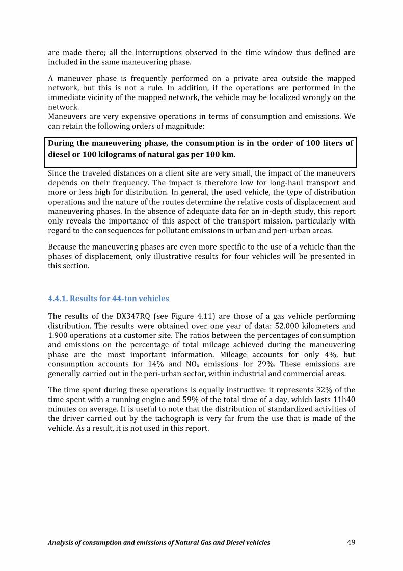
Analysis of consumption and emissions of Natural Gas and Diesel vehicles 49
are made there; all the interruptions observed in the time window thus defined are included in the same maneuvering phase.
A maneuver phase is frequently performed on a private area outside the mapped network, but this is not a rule. In addition, if the operations are performed in the immediate vicinity of the mapped network, the vehicle may be localized wrongly on the network. Maneuvers are very expensive operations in terms of consumption and emissions. We can retain the following orders of magnitude:
During the maneuvering phase, the consumption is in the order of 100 liters of
diesel or 100 kilograms of natural gas per 100 km.
Since the traveled distances on a client site are very small, the impact of the maneuvers depends on their frequency. The impact is therefore low for long-haul transport and more or less high for distribution. In general, the used vehicle, the type of distribution operations and the nature of the routes determine the relative costs of displacement and maneuvering phases. In the absence of adequate data for an in-depth study, this report only reveals the importance of this aspect of the transport mission, particularly with regard to the consequences for pollutant emissions in urban and peri-urban areas.
Because the maneuvering phases are even more specific to the use of a vehicle than the phases of displacement, only illustrative results for four vehicles will be presented in this section.
4.4.1. Results for 44-ton vehicles
The results of the DX347RQ (see Figure 4.11) are those of a gas vehicle performing distribution. The results were obtained over one year of data: 52.000 kilometers and 1.900 operations at a customer site. The ratios between the percentages of consumption and emissions on the percentage of total mileage achieved during the maneuvering phase are the most important information. Mileage accounts for only 4%, but consumption accounts for 14% and NOx emissions for 29%. These emissions are generally carried out in the peri-urban sector, within industrial and commercial areas.
The time spent during these operations is equally instructive: it represents 32% of the time spent with a running engine and 59% of the total time of a day, which lasts 11h40 minutes on average. It is useful to note that the distribution of standardized activities of the driver carried out by the tachograph is very far from the use that is made of the vehicle. As a result, it is not used in this report.

Analysis of consumption and emissions of Natural Gas and Diesel vehicles 50
Figure 4.11: Maneuvering phases of the DX347RQ – NGV – Distribution
The number of customers (break in the total laden weight) per 100 kilometers is 3.6.
For comparison, we present the results for the DY491CV which is a vehicle of the same model as the DX347RQ and which also carries out distribution missions, but in another geographical area and for another customer. We then obtain quite different figures. Mileage counts for 2%, consumption for 8% and NOx emissions for 15%. For the duration of the day on average of 11:00 hours, the time spent on the customer sites is lower. Finally, the traveled distance between two maneuvering phases goes from 30 kilometers for the first vehicle to 80 kilometers for the second.
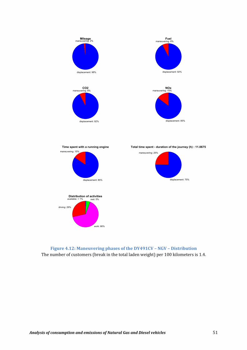
Analysis of consumption and emissions of Natural Gas and Diesel vehicles 51
Figure 4.12: Maneuvering phases of the DY491CV – NGV – Distribution
The number of customers (break in the total laden weight) per 100 kilometers is 1.4.

Analysis of consumption and emissions of Natural Gas and Diesel vehicles 52
The last semi-trailer presented is a diesel engine mainly performing long-haul missions. Mileage counts for 1%, consumption for 3% and NOx emissions for 11%. The very high ratio of NOx emissions percentage to percentage of mileage is due to highway trips where emissions are very low.
Figure 4.13: Maneuvering phases of the DE477VE – DIESEL – Long-haul
The number of customers (break in the total laden weight) per 100 kilometers is 1.0.

Analysis of consumption and emissions of Natural Gas and Diesel vehicles 53
4.4.2. Results for 19-ton vehicles
The results for a 19-ton rigid truck differ completely from those obtained for 44-ton semi-trailers: maneuvers or deliveries are less expensive. The basic reason is that the maneuver of a rigid medium-loaded vehicle does not compare to that of a heavily loaded semi-trailer. Mileage then counts for 2%, consumption for 6% and NOx emissions for 4%. These figures must however be compared with the 40 kilometers of distance traveled between two maneuvering phases, which characterize a distribution profile in peri-urban areas. The results would be different for a vehicle performing downtown distribution, with twice the number of stops and difficult parking conditions. For such vehicles, it is the delivery conditions - traffic conditions, parking conditions and traffic density - and not maneuvers – loading and docking – that are decisive.
The fact that the percentage obtained on NOx (4 %) is lower than that obtained for CO2 (6 %) is an anomaly which refers to the measurement problem mentioned in the second chapter: emissions are underestimated because the measurement is impossible during the first minutes after the start-up. Thus, in the present case, the measurement is only valid during 60% of the time spent in maneuvers, against 84% when we consider the time spent in the whole trip. This lack of measurement in the first moments after starting the engine is generalizable to the maneuvers of all vehicles. However, it is impossible to estimate precisely the impact on the total volume of emissions. It is very likely high for rigid trucks, for which the frequency of engine stops is high. At the opposite, it is possible that it is secondary for the semi-trailers with regard to the very high cost of maneuvers. To conclude in a general way, the description of the real operating conditions imposes the substitution of the concept of maneuvers by the more general one of deliveries, which concept includes the arrival on the site, the maneuvers, the stops of the engine, and the departure of the site.

Analysis of consumption and emissions of Natural Gas and Diesel vehicles 54
Figure 4.14: Maneuvering phases of the EB539DE – NGV rigid truck – Distribution
The number of customers (break in the total laden weight) per 100 kilometers is 2.5.
4.5. The wind
A headwind has a negative effect sufficiently pronounced and sufficiently known to lead drivers to adopt a dangerous “platooning” strategy : they follow the downstream vehicle closely to make a screen. At the request of the carriers, we therefore tried to measure the effect of the wind. The study that follows focuses on the impact of the intensity of a steady wind, either front or back, on consumption and emissions. We do not study the effect of a side wind or the effect of wind gusts.
This study was carried out on the A7 motorway in the Rhône Valley where the orientation of the road is generally parallel to the wind direction. The first sector selected was a stretch of about 40 km between Orange and Montélimar. The choice of this sector was motivated by two reasons:
a stable speed is observed on a relatively flat section; we have an average slope of less than 1 ‰
there is free access to meteorological data from the Montélimar station, located a little further north
The path presented below is a typical path, knowing that each path may have slight variations. The maximum slope of the downward path (see Figure 4.15) is 1% and the average slope is 1 ‰. The vehicles have a total laden weight ranging between 35 and 44 tons. Note that we have both a very stable speed and a significant variability of the mean consumption (between 20 and 30 kg / 100km) on sections of a length on the order of 2 km. The upward path is approximately symmetrical to the downward path, with a total laden weight ranging between 26 and 36 tons.

Analysis of consumption and emissions of Natural Gas and Diesel vehicles 55
Figure 4.15: Downward path – section Montélimar-Orange on the A7 highway
To confirm the initial results, which will be presented below, the study was then extended to a second sector, 25 kilometers long between Montélimar and Valence. We finally considered the complete path between Orange and Valence, a hundred kilometers long, including the Montélimar bypass. As the speed is less stable on the section around Montélimar, because of higher slopes and heavy traffic, the wind effect is relatively smaller.
4.5.1. Description of wind conditions in Montélimar
The study was conducted on a diesel vehicle that used this route for 21 months. Such a duration makes it possible to consider that the distribution of encountered meteorological conditions is statistically representative.
Figure 4.16 gives the wind distribution over the Montélimar station over a period of 21 months with a measurement per period of 3 hours. The prevailing wind is obviously the Mistral, which is not a north wind but a katabatic wind31 from north-west to north. The parallelism between the wind direction and the average orientation of the A7 motorway is therefore relative; moreover, locally, the orientation of the motorway deviates significantly from the North-South axis. We have therefore selected trips for which the wind is approximately North-South or South-North. Initially, a margin of tolerance of ±20 ° was used: it was extended to ± 30 ° without changing the results.
Over the twenty-one months of the project, there are 138 upward and 121 downward trips using the motorway stretch between Orange and Valence. The distributions of the total laden weight are different according to the direction of the trip. In order to eliminate the variability related to the total laden weight, the upward paths were
31 A katabatic wind is the consequence of a mass of cold air coming down from the mountains because of its weight.

Analysis of consumption and emissions of Natural Gas and Diesel vehicles 56
selected with a total laden weight ranging between 26 and 36 tons and downward paths with a total laden weight ranging between 35 and 44 tons . Depending on the case, the sample is reduced to 60 or 90 individuals. Finally, after filtering on the wind direction, the percentage of useful days varies between 60% and 90% of the population of the remaining population.
Figure 4.16: Distribution of the wind speed - station SYNOP at Montélimar Each point indicates the origin of the wind and the associated vector module indicates its speed (m / s)
Remember that, in general, wind conditions are seasonal. Thus in the Rhône corridor “the windiest period of the year lasts 5.7 months, from November 8 to April 28, with mean wind speeds greater than 13.9 kilometers per hour. The windiest day of the year is March 20th, with an average wind speed of 15.2 kilometers per hour.” This seasonality was not taken into account in this study.
4.5.2. Estimation of wind effects
From meteorological observations, speed and direction of the wind, a speed variable is defined whose sign depends on the trip: according to whether the vehicle encounters a tailwind or a headwind, the wind speed is considered as positive or negative. The consumption of the vehicle is thus negatively correlated with the wind speed. The mean consumption and the NOx emissions are then reported according to the wind speed. One figure is obtained for the downward trips and another for the upward trips.
The results (see Figure 4.17) show that the wind has no visible effect on NOx emissions: the distribution of emissions is independent of the mean wind speed. This is explained by the fact that a moderate steady wind does not involve strong and sudden acceleration.

Analysis of consumption and emissions of Natural Gas and Diesel vehicles 57
Figure 4.17: Wind effects on downward trips
Figure 4.18: Wind effects on upward trips
To quantify the impact of the wind, a linear regression was performed to explain the consumption as a function of wind speed. The regression line has been added to each figure; performing two independent regressions according to the sign of the wind speed was not relevant. From the regression, we obtain an estimate of the theoretical consumption for a zero wind and for the extreme values of the speed. The relative amplitude of the variation is defined from the ratio of consumption for maximum wind to consumption for zero wind. For Figure 4.17 these amplitudes are [-14%, + 8%]. Table 4.5 shows the results on the Orange-Montélimar, Montélimar-Valence and Orange-Valence sections. The fundamental result is the asymmetry of the amplitudes according to whether the path is ascending or descending; the existence of a coupling between the effect of the wind and that of the elevation difference seems likely. Note that the assumed effect of the average total laden weight, which is greater in the downward direction (40 t vs. 31 t), is erased from that of the wind: the most loaded vehicle consumes less.

Analysis of consumption and emissions of Natural Gas and Diesel vehicles 58
Upward trips Downward trips
Orange - Montélimar-South 36 % 20 % Montélimar-Noth - Valence 36 % 28 % Orange-Valence
any slope unstabilized speed
30 %
24 %
Table 4.5: Relative amplitude of change in consumption
Note that the wind speed range are identical for upward and downward trips.
The meteorological observations on both populations (see Figures 4.17 and 4.18) show a maximum wind speed of 12 m / s in the North-South direction and 6 m / s in the South-North direction. If the maximum speeds were 12 m / s in both directions, the maximum amplitude of variation would no longer be [-14%, + 22%] but [-22%, + 22%]. Moreover the wind speed extreme values observed on the sample are lower than the maximum values observed in the Rhone Valley. Finally, we must add that the direction of the wind is not strictly parallel to the axis of the road. Therefore maximum amplitude of wind effects would therefore be even greater, while remaining under normal operating conditions.
On this sample, we do not have high wind speeds: no wind speed exceeds 43.2 km / h32. The sample is nevertheless large enough to be statistically significant.
Finally, it should be noted that the wind speed distribution is relatively uniform (see the abscissa in Figures 4.17 and 4.18) and that therefore a strong wind is as likely as a weak wind.
4.6. Estimation of the engine temperature effects
Considering NOx emissions, the proper functioning of the pollution control systems of diesel vehicles and gas vehicles requires fairly high temperatures that are only reached respectively 20 and 2 minutes after starting the engine33. During this cold start phase, the emission rates are high enough that, despite the short duration, the contribution of this start-up phase can have a major impact. The objective of this part is to quantify this impact under real operating conditions.
As part of the Equilibre project, for 44-ton vehicles performing distribution, the mean distance traveled between two operations ranges between 30 and 60 km depending on the carriers. During a day, a vehicle that travels between 200 and 300 km makes several short trips. The time spent during stops ranges between 30 and 60% of the total time with an average time of 40 minutes per stop. This mean value should be compared to the time required to cool the engine and the pollution control system, which is 4 hours for a 32 A windsock is horizontal for a wind speed of 45 km / h, which is the limit for a wind that is considered strong for its effects on driving. According to Météo France, a violent and dangerous wind starts at 80 km / h. Still according to Météo France, the Mistral can blow on the plain up to 100 km / h. 33 Personal communication, Bernard Guiot (CRMT). These figures are likely to vary according to technological developments.

Analysis of consumption and emissions of Natural Gas and Diesel vehicles 59
diesel vehicle and 2 hours for a natural gas vehicle34. The conclusion is that, in the context of distribution missions, the engine temperature will have no effect apart from starting at the beginning of the day. The possibility of a second cold start therefore only arises for long-haul missions, for which we could observe a long-term stop in the middle of the day as part of a round trip. However, in practice, on twenty-one months of operation of a vehicle usually assigned to this type of mission, we observe only once such a long break... and it is not even during a long-haul mission. Going beyond these few observations, a trivial economic consideration leads to the conclusion that the case of a second cold start in the day can only be marginal because a carrier does not leave a vehicle unoccupied for 4 hours.
In theory, the study of cold starts would require a measurement of the temperature and more precisely of the temperature of the pollution control system. In practice, the Equilibre project only knows the oil, water and fuel temperatures. The detailed examination of the data shows that none of these temperatures is sufficiently correlated with the temperature of the pollution control system35. The results presented on cold starts therefore do not include any temperature measurement and the existence of a cold start is determined from the duration of the stopping of the vehicle. In practice, once the absence of a second cold start has been established, the absence of a measurement of the temperature of the pollution control system is not a problem (it is only to establish the inexistence of a second cold start that the absence of this measure was a handicap).
Figure 4.19 shows NOx emissions during the trip for a long-haul diesel vehicle. The start-up phase, associated with the first ten kilometers, accounts for 14% of the NOx emissions and for 2.3% of the mileage. As evidenced by the maximum speed value and its instability, this start-up phase is located on the outskirts of urban areas. There is also a slope of 2% on the last kilometers of this startup phase, which induces a high consumption. In this example, the emission rate therefore depends on the road category (ie. urban area), the elevation profile and finally the cold start.
34 Personal communication, Bernard Guiot (CRMT). 35 At start-up, the water temperature reaches a stable value in 10 minutes, while the NOx emission measurements show that the pollution control system of a diesel vehicle has not yet reached its optimal operating state.

Analysis of consumption and emissions of Natural Gas and Diesel vehicles 60
Figure 4.19: NOx emissions – DIESEL
So we looked for a second cold start made under different conditions. Figure 4.20 shows a second cold start in the middle of a trip, done on a national road; the situation is as complex as that encountered at the beginning of the day in the previous figure. This restart phase is characterized by the visible step on the cumulative emissions (located 105 km far from the departure), after which the slope returns to a normal value. During this phase, cumulative emissions are 30 grams; this value is similar to that observed at the beginning of the day
Figure 4.20: NOx emissions – cold start located at km 105 – DIESEL Trip Annecy-Thonon on main road. At km 105, the “jump” of cumulative NOx emissions (red curve in the bottom figure) is correlated with the restart after stopping for more than 4 hours (top figure).

Analysis of consumption and emissions of Natural Gas and Diesel vehicles 61
Eventually, for all trips, NOx emissions were measured over the first twenty minutes of the trip without seeking to isolate the explanatory factors: over the twenty-one months of the experiment, they vary between 20 and 30 grams and the mean value is 25 grams. Compared to 250 grams averaged over a full trip, this value means that the start-up phase accounts for 10% of NOx emissions; if we deduct what is specific to a start-up phase, generally carried out in peri-urban areas, the impact of a cold engine is still lower than this percentage. To summarize, compared to facilities, traffic, delivery conditions or wind conditions, cold start is only a secondary factor which has not been given priority in this project.
Compared with other explanatory factors, the cold start has a secondary impact on NOx emissions. In particular, the impact of the maneuvers is much higher than that of cold starts. However, this could be revised if measurements were available within the first few minutes after starting the engine.
4.7. Conclusion.
The fuel consumption and emissions of a vehicle depend on many explanatory factors whose effects are of the first order. Some of these factors are observable and predictable: road category, elevation profile and total laden weight. Some are observable but the information is not easily accessible, such as road facilities. Some depend on time: traffic conditions and weather conditions. These can be recurrent or otherwise unpredictable; knowing that we do not predict the consumption of a mission but the mean consumption of a series of identical missions, this predictability depends not only on the predictable nature of the events (congestion, rainfall, etc.) but also on the identity of temporal descriptions (hours, days, seasons) of the missions. To sum up:
the category of the road section, the elevation profile and the total laden weight being assumed to be identical, there remains a still important variability between trips. The density of facilities (eg. roundabout, speed bump, etc), which is correlated with the urbanization level, and the traffic density, which is also correlated with the urbanization level, are the main factors explaining this variance. In the case of distribution missions the frequency of loading and unloading operations is decisive. Uncommon factors36 that could be added to the study are beyond the scope of this project
there is an irreducible daily variability of consumption between two missions carried out on the same road and under similar conditions. When taking into account the road category, the elevation profile and the total laden weight, we will see later in the report that this daily variability is in
36 Road sinuosity, nature of the pavement and narrowness of a secondary road have a major effect; however, this will have a significant impact on the entire trip only for an uncommon mission where the trip is mainly on this type of road. Such a case was left out in this study.

Analysis of consumption and emissions of Natural Gas and Diesel vehicles 62
the order of ± 5% in a real operating situation, the study of secondary explanatory factors is
all the more difficult because it is generally impossible to control first-order factors
explanatory factors are frequently correlated with each other consumption and emissions are not mere sums of contributions from the
various explanatory factors; for instance, there are coupling effects between the elevation profile and the wind conditions or between the elevation profile and some facilities.

Analysis of consumption and emissions of Natural Gas and Diesel vehicles 63
5. Anomalies and dysfunctions
During the project, multiple malfunctions were noted, both on gas vehicles and on diesel vehicles: engine power drop, abnormal NOx emissions. These failures and malfunctions are part of the actual vehicle operating situation and this chapter looks at their impact on fuel consumption, emissions and vehicle availability. These malfunctions are generally caused by the vehicle, but the gas composition could be incriminated. These defects affected seven vehicles, belonging to five different models, out of the dozen of the project; it is recalled that all vehicles are commercial models and not prototypes; these defects have affected both a CNG vehicle, whose technology development is recent, a diesel vehicle and an LNG vehicle, whose technologies are more proven. The defects found are the following:
occasionnaly, a power drop on a gas vehicle systematicaly, unusually high NOx emissions on a diesel vehicle systematicaly, unusually high NOx emissions on two natural gas vehicles of the
same model occasionnaly, unusually high consumption and NOx emissions on an LNG vehicle
5.1. Power drop
On multiple occasions, when the maximum power of the engine was requested, a power deficit was observed by the driver on the vehicle DX347RQ equipped with a natural gas engine. A first step consisted in verifying this finding, characterizing it and quantifying it.
At first, the driver (ie. the driving style) was eliminated as the cause, because it was always the same driver who took the same path. In the same way, the fuel was put out of cause because no correlation could be established with the frequentation of a refueling station.
We have studied in detail the operation of the vehicle DX347RQ which has the particularity to be pushed in its limits in mountain paths. This drop in power was characterized and quantified on a typical route: the climb of Col d'Évires over a dozen kilometers.

Analysis of consumption and emissions of Natural Gas and Diesel vehicles 64
Figure 5.1: Climb of Col d'Évires – normal running
Figure 5.2: Climb of Col d'Évires – abnormal running The difference in operation can be seen in the upper graph where the power curve (in red) goes above the bar of 90% of the maximum power in Figure 5.1 and remains below in Figure 5.2. The other curves show the similarity of the use of the vehicle in both cases.
This malfunction results in the inability of the engine to provide a high power continuously: Figure 5.2 shows power peaks after a gear change and then a fall and finally a stabilization of the supplied power (a minimum duration of 20 seconds has been retained to characterize such a plateau). The difference between normal and abnormal operation can be seen by comparing the powers above the 225 kW line in

Analysis of consumption and emissions of Natural Gas and Diesel vehicles 65
Figures 5.1 and 5.2 – the nomimal power of the vehicle is 250 kW. So we compared the same trip on different days, made by the same vehicle and with the same driver. Table 5.1 shows the values for several days in March. Red days, with a total laden weight of approximately 33 tons , are defective days that can be compared to green days which are normal days. For the defective days, we note the inability of the vehicle to continuously support an indicated power of 225 kW. It is noted that this power deficit is observed only for a vehicle pushed into its limits: in this case a total laden weight of more than thirty tons with a mean slope of 2.5%.
The previous results were confirmed in November 2016 by assigning to the same trip a second vehicle of the same model: the DY491CV. The experiment lasted one week, from November 22 to 30, with two trips taking the Évires pass. On both paths crossing the pass one of the two shows the same operating anomalies as those observed with the DX347RQ.
DAY PTC (tons )
TRIP DURATION (sec)
DURATION SUCH POWER > 225 kW
DURATION SUCH POWER > 250 kW
2 31 701 253 55
3 19 606 21 0
7 33 725 0 0
8 21 678 44 0
9 34 747 0 0
11 33 722 64 0
16 34 739 95 0
18 33 693 223 0
22 18 595 120 23
23 33 765 213 117
24 21 633 81 0
25 33 688 349 51
31 27 639 277 53
Table 5.1: Power use – days of March 2016 green: normal days; red: abnormal days; black: days which are not relevant PTC: total laden weigth; DURATION: time taken by the vehicle to climb the pass; DURATION SUCH POWER > 225 kW: cumulative time, for which the indicated power exceeds 225 kW for at least 20 consecutive seconds. DURATION SUCH POWER > 250 kW: cumulative time, for which the indicated power exceeds 250 kW for at least 20 consecutive seconds.
Although the statistical data and figures reporting the power confirmed the feeling of the drivers, it is only the examination of the engine mapping that made it possible to characterize the malfunction37. The comparison of the maps shows the existence of two operating regimes for the defective days (see Figure 5.3).
37 Bruno Jeanneret of the Transport and Environment Laboratory (IFSTTAR) has significantly contributed to this work.

Analysis of consumption and emissions of Natural Gas and Diesel vehicles 66
Figure 5.3: Climb of Col d'Évires – normal running (left) and abnormal (right)
This data was transmitted to the manufacturer and a patch was returned in July 2017 as a modification of the calculator parameters.
A second series of observations was then made on new climbs at the Col d'Évires. These observations made between June and December 2017 are distributed before and after the intervention of the manufacturer. Since the indicators used in Table 5.2 do not have sufficient reliability, to qualify the new trips, we relied solely on a visual examination of the engine maps. This review confirmed that all trips after the patch are normal. A simple calculation makes it possible to estimate the probability that the improvement observed is not due to chance. Before modification, 5 malfunctions are observed on 12 observations. After modification, no dysfunction was observed on 8 observations. The probability of not observing any malfunction if the defect has not been corrected is (7/12)8 = 0.013. Although this value is very low, it cannot be totally ruled out that the defect remains.
DAY PTC (tons )
TRIP DURATION (sec)
DURATION SUCH POWER > 225 kW
DURATION SUCH POWER > 250 kW
2 march 2016 31 701 253 55
7 33 725 0 0
9 34 747 0 0
11 33 722 64 0
16 34 739 95 0
18 33 693 223 0
23 33 765 213 117
25 33 688 349 51
12 june 2017 32 762 304 84
21 june 2017 36 691 376 132
23 june 2017 39 875 154 22
03 july 2017 36 710 303 103
17 july 2017 35 747 235 0
18 july 2017 31 642 238 0
24 july 2017 37 753 376 0
31 july 2017 36 730 361 29
16 august 2017 36 741 259 0
21 august 2017 34 679 317 36
22 nov. 2017 37 706 408 91
26 dec. 2017 37 749 369 22
Table 5.2: Power use on relevant observations (total laden weight > 30 tons ) red / brown: before intervention (normal / dysfunction); green: after intervention

Analysis of consumption and emissions of Natural Gas and Diesel vehicles 67
This example reflects the difficulty of objectively characterizing a minor flaw - but nevertheless easily detected by the drivers. We should note that over twenty-one months of experimentation in real operating situation, only 20 trips were made under almost identical conditions. It then took a year between detection and correction.
5.2. NOx emissions of a diesel vehicle
From the beginning of the project, over a period of six months, the average NOx emissions of one diesel vehicle were two to three times higher than those of other vehicles. The vehicle in question is DL928LJ (see Table 5.3).
Since this malfunction had no other visible impact on fuel consumption or engine power, the phenomenon remained unnoticed by drivers and carriers. It was only revealed by emission measurements.
Motorway Country road Urban expressway
Urban crossing
Dense urban area
DE477VE 34 81 - 112 125 DS282LC 32 124 - 117 - DL928LJ 118 234 - 279 367
Table 5.3: NOx emissions (g/100 km)
These data were transmitted to the manufacturer and a heavy intervention was carried out in May 2017. Without going into the details of the intervention, many elements of the pollution control system, which would have undergone accelerated degradation, have been replaced. The cause was an oil leak at the turbo-compressor, which deteriorated the catalyst.
Motorway Country road
Urban expressway
Urban crossing
Dense urban area
DE477VE (6 months) 34 81 - 112 125 DE477VE (21 months) 41 101 31 129 142 DS282LC (6 months) 32 124 - 117 - DS282LC (12 months) 41 121 - 126 - DL928LJ (before, 6 months) 118 234 - 279 367 DL928LJ (after, 5 months) 51 86 50 140 190
Tableau 5.4: NOx emissions (g/100 km)
A second measurement campaign was carried out after the correction. This has been effective since NOx emissions have decreased by a factor of about two and are now comparable to those of other vehicles (see Table 5.4). We check that this improvement is not a coincidence by comparing the results obtained on other diesel vehicles. Thus, for the DE477VE and the DS282LC, the comparison of emissions over two periods reveals a variability of between ten and twenty percent; comparatively, the hundred percent gain obtained on the DL928LJ cannot be explained by natural variability.

Analysis of consumption and emissions of Natural Gas and Diesel vehicles 68
In the rest of the report, the question of the presentation of the statistics relating to the vehicle arose: separate data for each period; aggregated data for both periods; data including only the period after correction of the defect. The third solution was chosen to facilitate the comparative reading of results all associated with roadworthy vehicles.
Given a vehicle and a road category, the variability of emissions between two measurement periods is an indication of the uncertainty in the values. Since NOx emissions are very sensitive to transient phenomena, linked to unobserved explanatory factors, this variability could easily be explained by differences in operating conditions: facilities, traffic conditions and weather conditions. This issue has been studied in more detail in the previous chapter.
5.3. NOx emissions of natural gas vehicles
As for the diesel vehicle studied in the previous paragraph, mean NOx emissions of a vehicle gas model were much higher than those of other CNG vehicles. These high emissions were observed under conditions of unstable speed: urban crossing, dense urban and country road. The two vehicles in question are the EL375RS and the EN052KT (see Table 5.5)
These data were transmitted to the manufacturer and several interventions were carried out from February 2018. The intervention was limited to a new setting of the computer for the first vehicle. For the second vehicle, in addition to the new tuning of the computer software, many elements of the pollution control system and exhaust have been replaced. The cause would be a manufacturing defect.
Motorway Country road Urban expressway
Urban crossing
Dense urban area
DX347RQ 14 28 22 46 50 DY491CV 20 19 21 41 48 EA190HL (*) 18 93 14 137 157 EL375RS (before) 6 96 34 130 226 EN052KT (before) 12 79 33 180 293
EL375RS (after, 40 days) 6 80 24 96 210 EN052KT (after, 10 days) 13 79 15 161 287
Table 5.5: NOx Emissions (g/100 km) DX347RQ and DY491CV are CNG vehicle. EA190HL which is an LNG vehicle. EL375RS and EN05KT are LNG+CNG vehicle. The first one operates at 95% LNG, whereas the second operates at 100 % CNG.
Measurement campaigns were taken after these corrections, with respectively 40 and 10 days of effective operation for these two vehicles. At first glance, both for the EL375RS and for the EN052KT, the data in Table 5.5 show no improvement after the manufacturer's corrections
the results on motorway, on country road and in dense urban areas are stable: we saw in § 5.2 that under similar conditions a variability of 10 to 20% is natural
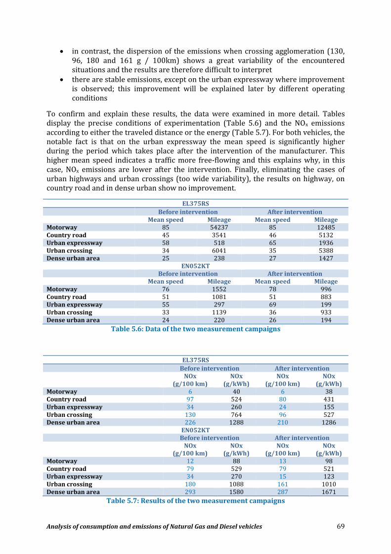
Analysis of consumption and emissions of Natural Gas and Diesel vehicles 69
in contrast, the dispersion of the emissions when crossing agglomeration (130, 96, 180 and 161 g / 100km) shows a great variability of the encountered situations and the results are therefore difficult to interpret
there are stable emissions, except on the urban expressway where improvement is observed; this improvement will be explained later by different operating conditions
To confirm and explain these results, the data were examined in more detail. Tables display the precise conditions of experimentation (Table 5.6) and the NOx emissions according to either the traveled distance or the energy (Table 5.7). For both vehicles, the notable fact is that on the urban expressway the mean speed is significantly higher during the period which takes place after the intervention of the manufacturer. This higher mean speed indicates a traffic more free-flowing and this explains why, in this case, NOx emissions are lower after the intervention. Finally, eliminating the cases of urban highways and urban crossings (too wide variability), the results on highway, on country road and in dense urban show no improvement.
EL375RS
Before intervention After intervention Mean speed Mileage Mean speed Mileage
Motorway 85 54237 85 12485 Country road 45 3541 46 5132 Urban expressway 58 518 65 1936 Urban crossing 34 6041 35 5388 Dense urban area 25 238 27 1427
EN052KT Before intervention After intervention Mean speed Mileage Mean speed Mileage
Motorway 76 1552 78 996 Country road 51 1081 51 883 Urban expressway 55 297 69 199 Urban crossing 33 1139 36 933 Dense urban area 24 220 26 194
Table 5.6: Data of the two measurement campaigns
EL375RS
Before intervention After intervention NOx
(g/100 km) NOx
(g/kWh) NOx
(g/100 km) NOx
(g/kWh) Motorway 6 40 6 38 Country road 97 524 80 431 Urban expressway 34 260 24 155 Urban crossing 130 764 96 527 Dense urban area 226 1288 210 1286
EN052KT Before intervention After intervention NOx
(g/100 km) NOx
(g/kWh) NOx
(g/100 km) NOx
(g/kWh) Motorway 12 88 13 98 Country road 79 529 79 521 Urban expressway 34 270 15 123 Urban crossing 180 1088 161 1010 Dense urban area 293 1580 287 1671
Table 5.7: Results of the two measurement campaigns

Analysis of consumption and emissions of Natural Gas and Diesel vehicles 70
In conclusion, despite the numerous interventions by the manufacturer no reduction in NOx emissions could be observed on these two vehicles of the same model. Therefore, the periods before and after intervention will not be separated in the rest of the report
5.4. Consumption and NOx emissions of a natural gas vehicle – LNG
Over a ten-day period in October 2017, the driver detected a decline in the performance of his LNG vehicle. The vehicle in issue is EA190HL.
After signaling the malfunction, some defective hardware elements were immediately replaced by the manufacturer and a return to normal was found. Subsequently and independently, an analysis of the NOx emission identified this phase of dysfunction: the mean emission rate is 56 grams per hundred kilometers in normal period and 197 grams during the malfunction period (see Figure 5.4). Over the twenty-one months of the duration of the experiment, this phase of over-emission will have increased by only 6% the total quantity of emitted NOx.
Figure 5.4: Trips during the period ranging between august 2017 to january 2018 - LNG The reported days are those when the vehicle engine was started. Days with zero value were
eliminated because the mileage was too small (less than 60 km) under generally exceptional
conditions (tractor without trailer). We thus finally obtain 106 operational days over a period of
6 months.
In the remainder of the report, the question of the presentation of the statistics relating to the vehicle arose. Since the nature of the malfunction was not the same as for the DL928LJ (a very long dysfunctioning), the answer was different. Because the objective of the project is the presentation of results in real operating situation and because a
Analysis of consumption and emissions of Natural Gas and Diesel vehicles 71
punctual failure is part of the daily life of a vehicle, we chose to present data including the period of the breakdown.
5.5. Conclusions
The characterization of malfunctions is tackled from different angles: the origin of the defect, the severity and the duration. The origin of the fault and the seriousness of the malfunction are the sole responsibility of the manufacturer; the duration of the malfunction depends on the time required before the correction but also the time necessary for its detection. The defect may be an occasional failure of a hardware element, related to a specific history, or result of either a design defect or a manufacturing defect. The difference between occasional failure and design or manufacturing defects is the systematic nature of the defect in the last two cases. They affect a fleet of vehicles and not just one. The issue of the time required to correct failures or design flaws is beyond the scope of this study. The only observation is that these delays are generally long and that the malfunctions therefore persist. The question of the time required to detect the defect is more interesting. If the malfunction does not affect engine power or consumption, it will not be detected by the driver or carrier. This was the case for the DL928LJ. Under actual operating conditions, such a defect can be found only during a technical visit.
The sample size is too small to obtain a representative statistics of the fleet of vehicles in service, this report does not attempt to estimate the environmental impact of such defects.
Analysis of consumption and emissions of Natural Gas and Diesel vehicles 72
6. Results for 44-ton semi-trailers
The presentation of the statistical results is divided into three main parts. The first characterizes the trips. The second part presents separately the consumption for diesel vehicles and for gas vehicles. No comparison of energy efficiency is made because such a study should be done from “well to wheel”, which is beyond the scope of this project. The third part compares the CO2 and NOx emissions of diesel and natural gas vehicles.
6.1. Trips characterization
Rather than a comparison of two motorizations, the Equilibre project compares uses and specifically the uses of diesel vehicles to those of natural gas vehicles. The traveled kilometers on each road category characterize these uses. Long-haul vehicles operate mainly on motorways, while vehicles that make distribution circulate mainly on country roads or in urban areas; as a rule, diesel vehicles are assigned to long-haul trips, while natural gas vehicles are assigned to distribution missions (see Figures 6.1 and 6.2). Not only are there exceptions, but the same vehicle can be assigned to missions of different kinds during the year; for example, the EL375RS is a gas vehicle performing long-haul trips, while the DL928LJ is a diesel vehicle that has gone from long-haul to distribution during the project.
The traveled kilometers on each road category are indicators of the representativeness of the displayed results (see Table 6.1). Of course, low mileage has led to ignoring consumption and emission measures, but since the distribution of transport missions is not random, high mileage is not a guarantee of statistical representativeness. The ideal case is one in which a vehicle uses a wide variety of roads and schedules; the reality is closer to the case of the vehicle which in the year makes 52 times the same trip with the same schedule.
Due to intra-class variability, the road is not sufficient information to interpret the results. Three variables characterizing the traveled distance on some road category were thus added: cumulative positive elevation, mean speed and number of “stop & go”.
A high accumulation of positive elevations implies a high consumption. Theoretically this criterion has a strong relative impact for country road and motorway. In practice, perhaps because all the vehicles operate in the same geographic areas, it has hardly been possible to discriminate between uses over very long periods (see Table 6.2).
The last two variables are indicators of the severity of the operating conditions, mainly in urban areas: a low average speed indicates a dense traffic, while a high number of “stop & go” indicates a high density of facilities involving stops. These criteria are clearly correlated (see Tables 6.3 and 6.4). The “stop & go” criterion, with values that can differ by a ratio of 1 to 5, proves decisive for a more precise characterization of urban trips.
The explanation of the observed values may be complex. For instance, when crossing urban areas, the number of “stop & go” may be higher for long-haul vehicles than for vehicles that make distribution. The explanation is that for the former this category

Analysis of consumption and emissions of Natural Gas and Diesel vehicles 73
corresponds to deliveries on the outskirts of large cities, while for the latter this category also includes many crossings of small towns without any stop.
Figure 6.1: Distributions of mileage – DIESEL
59% 15%
9%
10% 7%
DL928LJ
77%
7%
2% 13%
1%
DE477VE
83%
4% 13%
DS282LC
77%
7%
2% 13%
1%
EM644EF

Analysis of consumption and emissions of Natural Gas and Diesel vehicles 74
Figure 6.2: Distributions of mileage – NGV
EA190HL is a LNG vehicle.
17%
21%
56%
6%
DX347RQ
18%
35%
1%
40%
6%
DY491CV
84%
5% 1%
10%
EL375RS
33%
26% 7%
29%
5%
EN052KT
71%
10%
9%
2%
8%
EA190HL

Analysis of consumption and emissions of Natural Gas and Diesel vehicles 75
DIESEL
DL928LJ before the patch
DL928LJ after the patch
DE477VE DS282LC EM644EF
Motorway 70782 16779 139152 25187 50061 Country road 17295 6516 12978 1201 4405 Urban expressway 10561 2502 4133 69 1277 Urban crossing 12209 6753 23837 3980 8430 Dense urban area 8104 1787 1470 203 431
GAZ
DX347RQ DY491CV EL375RS EN052KT EA190HL Motorway 14531 12606 73425 4683 100814 Country road 17883 24257 4843 3681 13915 Urban expressway 56 605 641 981 12566 Urban crossing 47899 27738 8468 4006 3246 Dense urban area 5194 4249 292 757 10763
Table 6.1: Mileage
Mileage shown in red is statistically unrepresentative.
DIESEL
DL928LJ before
the patch
DL928LJ after the
patch
DE477VE DS282LC EM644EF
Motorway 0,8 - 0,5 0,7 0,5 Country road 0,6 - 0,9 0,8 0,8 Urban expressway 0,5 - 0,3 - 0,3 Urban crossing 0,5 - 0,9 1,5 1,1 Dense urban area 0,6 - 0,8 - 0,8
GAZ
DX347RQ DY491CV EL375RS EN052KT EA190HL Motorway 0,7 0,4 0,4 0,5 1,0 Country road 1,0 0,4 0,7 0,7 0,5 Urban expressway - 0,4 0,3 0,5 0,5 Urban crossing 1,1 0,5 0,6 0,7 0,7 Dense urban area 1,5 0,4 - 0,4 0,5
Table 6.2: Ratio of cumulative positive elevations over traveled distance (%)
In urban areas, because of the small length of the sections and the inaccuracy of the altimetry, the high values are unreliable (Urban crossing and Dense urban area). Considering a total elevation difference of zero for each road category, the mean slopes (in %) are twice the values indicated in the table. On the motorway, the EA190HL, with a mean slope of 2%, is clearly distinguishable from the DE477VE, with a mean slope of 1%. The first has circulated a lot in Auvergne (mountainous) while the second has mostly circulated in the Rhône Valley.

Analysis of consumption and emissions of Natural Gas and Diesel vehicles 76
DIESEL
DL928LJ avant
révision
DL928LJ après
révision
DE477VE DS282LC EM644EF
Motorway 81 79 85 82 86 Country road 55 56 51 58 51 Urban expressway 70 65 69 - 67 Urban crossing 40 41 43 42 44 Dense urban area 29 28 34 - 32
GAZ
DX347RQ DY491CV EL375RS EN052KT EA190HL Motorway 81 77 85 77 78 Country road 56 61 45 52 51 Urban expressway - 67 59 64 74 Urban crossing 45 41 34 35 37 Dense urban area 39 32 - 26 27
Table 6.3: Mean speed (km/h)
Below 30 km / h (in red) the operating conditions are considered severe.
DIESEL
DL928LJ avant
révision
DL928LJ après
révision
DE477VE DS282LC EM644EF
Motorway - 2 1 1 0 Country road - 7 18 6 13 Urban expressway - 6 5 - 4 Urban crossing - 42 47 62 37 Dense urban area - 140 86 - 81
GAZ
DX347RQ DY491CV EL375RS(*) EN052KT EA190HL Motorway 2 4 1 2 1 Country road 15 3 18 8 9 Urban expressway - 6 18 16 1 Urban crossing 41 41 95 85 38 Dense urban area 61 31 - 118 139
Table 6.4: Number of « stop & go » per hundred kilometers
Beyond 100 stops (in red) the operating conditions are considered severe. (*) EL375RS performs long-haul missions.

Analysis of consumption and emissions of Natural Gas and Diesel vehicles 77
In the course of this report, the mean total laden weight was rarely mentioned. There are three reasons for this absence. The first is that it is not a direct causal factor: it only really impacts consumption if it is coupled with elevation difference or acceleration. The second reason is that it hardly discriminates the uses. Thus, Table 6.5 reveals fairly similar values for all vehicles. The third reason is that this value is an average between full load trips and no-load trips38. Note that empty trips are not only empty returns, but also movements from the carrier’s depot to a customer’s loading site or from a customer’s delivery site to another customer’s loading site. This proportion of empty trips varies according to the type of mission and the road category (see Table 6.6); this must be taken into account when comparing the mean weights of distribution missions with those of long-haul missions. It should be noted that the proportion of empty displacements is never negligible. This aspect of the transport missions was not studied during the project.
Although the heterogeneity of the total laden weight according to the road category is low, it is not the effect of fluctuations; we will see later that 19-ton rigid trucks do not display such heterogeneity. A semi-trailer may have different route selection strategies - or imposed routes - depending on the traveled distance or the current operation: transportion, empty return, rallying a loading point, moving without a trailer, short trips, etc
DIESEL
DL928LJ
avant révision
DL928LJ après
révision
DE477VE DS282LC EM644EF
Motorway 26 - 32 24 29
Country road 23 - 27 24 26
Urban expressway 24 - 30 - 31
Urban crossing 17 - 27 24 26
Dense urban area 23 - 25 - 23
GAZ
DX347RQ DY491CV EL375RS EN052KT EA190HL
Motorway 24 25 29 - 26
Country road 20 24 24 - 25
Urban expressway - 25 25 - 25
Urban crossing 25 24 21 - 25
Dense urban area 19 25 - - 25
Table 6.5: Total laden weight (tons )
38 A mean total laden weight of 30 tons cannot account for one displacement with a total weight of 15 tons and two trips with a total weight of 37.5 tons ?
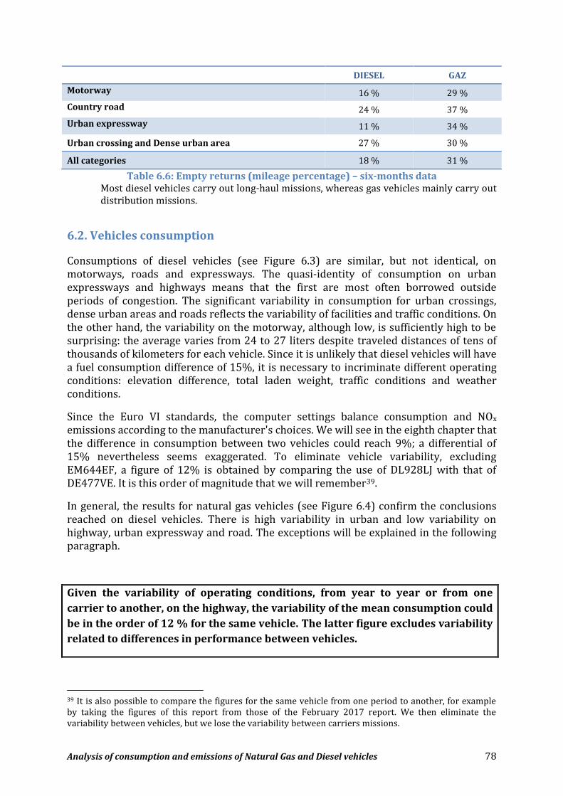
Analysis of consumption and emissions of Natural Gas and Diesel vehicles 78
DIESEL GAZ
Motorway 16 % 29 %
Country road 24 % 37 %
Urban expressway 11 % 34 %
Urban crossing and Dense urban area 27 % 30 %
All categories 18 % 31 %
Table 6.6: Empty returns (mileage percentage) – six-months data Most diesel vehicles carry out long-haul missions, whereas gas vehicles mainly carry out distribution missions.
6.2. Vehicles consumption
Consumptions of diesel vehicles (see Figure 6.3) are similar, but not identical, on motorways, roads and expressways. The quasi-identity of consumption on urban expressways and highways means that the first are most often borrowed outside periods of congestion. The significant variability in consumption for urban crossings, dense urban areas and roads reflects the variability of facilities and traffic conditions. On the other hand, the variability on the motorway, although low, is sufficiently high to be surprising: the average varies from 24 to 27 liters despite traveled distances of tens of thousands of kilometers for each vehicle. Since it is unlikely that diesel vehicles will have a fuel consumption difference of 15%, it is necessary to incriminate different operating conditions: elevation difference, total laden weight, traffic conditions and weather conditions.
Since the Euro VI standards, the computer settings balance consumption and NOx emissions according to the manufacturer's choices. We will see in the eighth chapter that the difference in consumption between two vehicles could reach 9%; a differential of 15% nevertheless seems exaggerated. To eliminate vehicle variability, excluding EM644EF, a figure of 12% is obtained by comparing the use of DL928LJ with that of DE477VE. It is this order of magnitude that we will remember39.
In general, the results for natural gas vehicles (see Figure 6.4) confirm the conclusions reached on diesel vehicles. There is high variability in urban and low variability on highway, urban expressway and road. The exceptions will be explained in the following paragraph.
Given the variability of operating conditions, from year to year or from one
carrier to another, on the highway, the variability of the mean consumption could
be in the order of 12 % for the same vehicle. The latter figure excludes variability
related to differences in performance between vehicles.
39 It is also possible to compare the figures for the same vehicle from one period to another, for example by taking the figures of this report from those of the February 2017 report. We then eliminate the variability between vehicles, but we lose the variability between carriers missions.

Analysis of consumption and emissions of Natural Gas and Diesel vehicles 79
Figure 6.3: Consumption of diesel vehicles The DL928LJ's fuel consumption and emissions data include only the period after the manufacturer's intervention.
26
35
26
37
44
0
5
10
15
20
25
30
35
40
45
50
Conso (l/100km)
DL928LJ
27
36
25
40 38
0
5
10
15
20
25
30
35
40
45
50
Conso (l/100km)
DE477VE
25
32 34
0
5
10
15
20
25
30
35
40
45
50
Conso (l/100km)
DS282LC
24
31
22
35 34
0
5
10
15
20
25
30
35
40
45
50
Conso (l/100km)
EM644EF

Analysis of consumption and emissions of Natural Gas and Diesel vehicles 80
Figure 6.4: Consumption of natural gas vehicles The consumption and emission data for the EL375RS and EN052KT vehicles include the entire experimental period since the manufacturer's intervention produced no improvement.
Further examination of the results for gas vehicles reveals some anomalies that require explanation.
24 27
0
36 35
0
5
10
15
20
25
30
35
40
45
50
Consommation (kg/100km)
DX347RQ
21
26
20
33
39
0
5
10
15
20
25
30
35
40
45
50
Consommation (kg/100km)
DY491CV
27
35
25
32
0 0
5
10
15
20
25
30
35
40
45
50
Consommation (kg/100km)
EL375RS
25 28
23
31
36
0
5
10
15
20
25
30
35
40
45
50
Consommation (kg/100km)
EN052KT
29
38
21
33 37
0
5
10
15
20
25
30
35
40
45
50
Consommation (kg/100km)
EA190HL
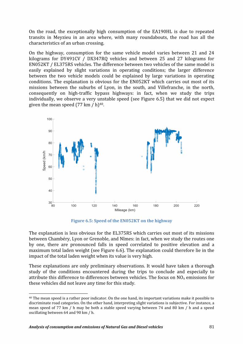
Analysis of consumption and emissions of Natural Gas and Diesel vehicles 81
On the road, the exceptionally high consumption of the EA190HL is due to repeated transits in Meyzieu in an area where, with many roundabouts, the road has all the characteristics of an urban crossing.
On the highway, consumption for the same vehicle model varies between 21 and 24 kilograms for DY491CV / DX347RQ vehicles and between 25 and 27 kilograms for EN052KT / EL375RS vehicles. The difference between two vehicles of the same model is easily explained by slight variations in operating conditions; the larger difference between the two vehicle models could be explained by large variations in operating conditions. The explanation is obvious for the EN052KT which carries out most of its missions between the suburbs of Lyon, in the south, and Villefranche, in the north, consequently on high-traffic bypass highways: in fact, when we study the trips individually, we observe a very unstable speed (see Figure 6.5) that we did not expect given the mean speed (77 km / h)40.
Figure 6.5: Speed of the EN052KT on the highway
The explanation is less obvious for the EL375RS which carries out most of its missions between Chambéry, Lyon or Grenoble, and Nîmes: in fact, when we study the routes one by one, there are pronounced falls in speed correlated to positive elevation and a maximum total laden weight (see Figure 6.6). The explanation could therefore lie in the impact of the total laden weight when its value is very high.
These explanations are only preliminary observations. It would have taken a thorough study of the conditions encountered during the trips to conclude and especially to attribute this difference to differences between vehicles. The focus on NOx emissions for these vehicles did not leave any time for this study.
40 The mean speed is a rather poor indicator. On the one hand, its important variations make it possible to discriminate road categories. On the other hand, interpreting slight variations is subjective. For instance, a mean speed of 77 km / h may be both a stable speed varying between 74 and 80 km / h and a speed oscillating between 64 and 90 km / h.
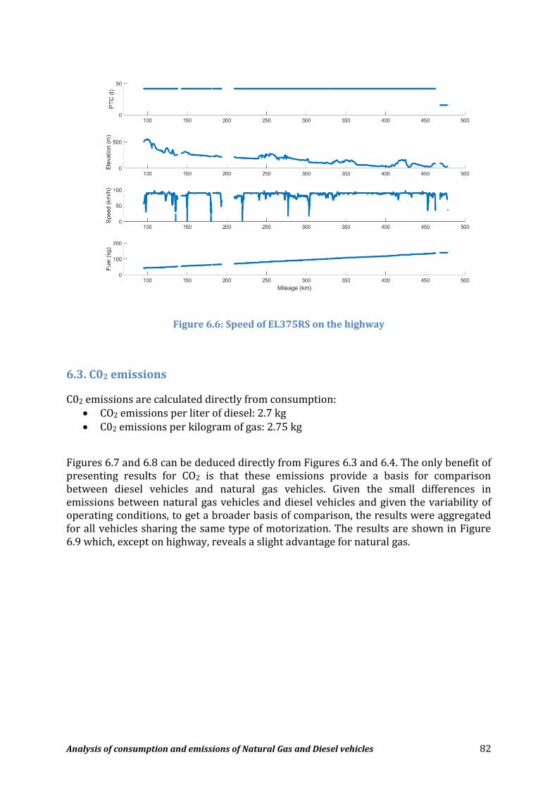
Analysis of consumption and emissions of Natural Gas and Diesel vehicles 82
Figure 6.6: Speed of EL375RS on the highway
6.3. C02 emissions
C02 emissions are calculated directly from consumption: CO2 emissions per liter of diesel: 2.7 kg C02 emissions per kilogram of gas: 2.75 kg
Figures 6.7 and 6.8 can be deduced directly from Figures 6.3 and 6.4. The only benefit of presenting results for CO2 is that these emissions provide a basis for comparison between diesel vehicles and natural gas vehicles. Given the small differences in emissions between natural gas vehicles and diesel vehicles and given the variability of operating conditions, to get a broader basis of comparison, the results were aggregated for all vehicles sharing the same type of motorization. The results are shown in Figure 6.9 which, except on highway, reveals a slight advantage for natural gas.

Analysis of consumption and emissions of Natural Gas and Diesel vehicles 83
Figure 6.7: C02 emissions - DIESEL The DL928LJ's fuel consumption and emissions data include only the period after the manufacturer's intervention.
70
95
70
100
119
0
20
40
60
80
100
120
140
CO2 (kg/100km)
DL928LJ
73
96
68
107 104
0
20
40
60
80
100
120
140
CO2 (kg/100km)
DE477VE
68
86 91
0
20
40
60
80
100
120
140
CO2 (kg/100km)
DS282LC
66
83
60
96 90
0
20
40
60
80
100
120
140
CO2 (kg/100km)
EM644EF

Analysis of consumption and emissions of Natural Gas and Diesel vehicles 84
Figure 6.8: C02 emissions – NGV
65 73
98 97
0
20
40
60
80
100
120
140
Emission CO2 (kg/100km)
DX347RQ
57
71
55
90
108
0
20
40
60
80
100
120
140
Emission CO2 (kg/100km)
DY491CV
75
95
68
88
0
20
40
60
80
100
120
140
Emission CO2 (kg/100km)
EL375RS
68 77
64
86 98
0
20
40
60
80
100
120
140
Emission CO2 (kg/100km)
EN052KT
79
103
58
91 102
0
20
40
60
80
100
120
140
Emission CO2 (kg/100km)
EA190HL

Analysis of consumption and emissions of Natural Gas and Diesel vehicles 85
Figure 6.9: Comparative of C02 emissions
6.4. NOx emissions
Unlike consumption, NOx emissions from diesel vehicles vary significantly from one vehicle to another, regardless of the road category (see Figures 6.10 and 6.12). A priori, the operating conditions are still in question. This variability is explained by the greater sensitivity of the emissions to local factors (e.g. facilities, traffic conditions) not taken into account. This sensitivity of the emissions to any factor making the speed unstable also explains the high ratio between the emission rate in urban area and the emission rate on road.
Considering that the variability of operating conditions could explain differences
in NOx emission rates, the performance of diesel vehicles in real-life situations is
likely to be very similar41.
From an environmental point of view, it is the kilometer emission rate that is of interest because it accounts for the emissions produced on a road section, which depend on the vehicle and the surrounding conditions. The ratio between urban emission rates and the road emission rate is therefore very high. From the engine manufacturer's point of view, which evaluates the performance of a vehicle, it is the emission rate according to the power developed (kWh) which is of interest; this rate makes it possible to partially eliminate the differences related to some operating conditions. When the emission rate is expressed in mg / kWh, the ratio between the emission rate in urban areas and the road emission rate decreases, but it remains high42. That being said, in practice, the
41 This conclusion is also based on the fact that the vehicles are equipped with similar pollution control systems. DL928LJ and EM644EF are equipped with SCR (selective catalytic reduction system). The DS282LC and the DE477VE are equipped with SCR and EGR (exhaust gas recirculation system) 42 Not only would the emission rate be non-linearly dependent on power, but it would also depend on its variability. The emission rate per kWh would thus be lower at low power in stationary mode.
76 80
58
95 102
71
113
67
102 110
0
20
40
60
80
100
120
Classe 1 :Autoroute
Classe 2 : Routenationale
Classe 3 : Voierapide urbaine
Classe 4 :Traversée
d'agglomération
Classe 5 : ZoneUrbaine Dense
Emissions CO2 (kg/100km)
GNV
Diesel

Analysis of consumption and emissions of Natural Gas and Diesel vehicles 86
emission rates, whether expressed as a function of the traveled distance or the power developed, are strongly correlated.
Figure 6.10: NOx emissions (g/100km) - DIESEL
Except on highway, the NOx emissions of natural gas vehicles vary widely from one vehicle to another (see Figures 6.11 and 6.13) and this without it being possible to invoke the operating conditions: variations are in the order of 30% between diesel vehicles but in order of 300% between natural gas vehicles. Some natural gas vehicles should be incriminated for poor performance. Moreover, in urban areas, the emission rates of these offending vehicles are slightly higher than those of diesel vehicles (see Figures 6.10 and 6.11)43. On the other hand, the best natural gas vehicles have urban
43 The manufacturer has been alerted about this and patches have been made. A measurement campaign was therefore re-launched after the writing of this report; the results are reported in Appendix E. They do not call into question the general conclusions of this report, but show that the very high emission rates of the incriminated vehicles are partly due to more severe operating conditions.
51
86
50
140
190
0
50
100
150
200
250
300
350
NOx (g/100km)
DL928LJ
26
98
33
143
198
0
50
100
150
200
250
300
350
Nox (g/100km)
EM644EF
41
101
31
129 142
0
50
100
150
200
250
300
350
Nox (g/100km)
DE477VE
41
122
0
126
0 0
50
100
150
200
250
300
350
Nox (g/100km)
DS282LC

Analysis of consumption and emissions of Natural Gas and Diesel vehicles 87
emissions rates much lower than those of diesel vehicles: the rates range between 40 and 50 g / 100 km in urban versus 135 and 190 g / 100 km for diesel vehicles
Figure 6.11: NOx emissions (g/100km) - NGV
14 28
46 50
0
50
100
150
200
250
300
350
Emission NOx (g/100km)
DX347RQ
20 19 21 41 48
0
50
100
150
200
250
300
350
Emission NOx (g/100km)
DY491CV
6
96
34
130
0
50
100
150
200
250
300
350
Emission NOx (g/100km)
EL375RS
12
79
33
180
293
0
50
100
150
200
250
300
350
Emission NOx (g/100km)
EN052KT
18
93
14
137 156
0
50
100
150
200
250
300
350
Emission NOx (g/100km)
EA190HL

Analysis of consumption and emissions of Natural Gas and Diesel vehicles 88
Figure 6.12: NOx emissions (mg/kWh) - DIESEL
For the DX347RQ and DY491CV, which are vehicles of the same model, despite mileage exceeding ten thousand kilometers on highway and country road, we note a variability of emissions in the order of 50% (see Figure 6.11). This variability is to be compared to the 12% variability for consumption on the highway.
386 483
379
748 847
0
200
400
600
800
1000
1200
1400
1600
NOx (mg/kWh)
DL928LJ
316
592
255
681 772
0
200
400
600
800
1000
1200
1400
1600
NOx (mg/kWh)
DE477VE
326
769 745
0
200
400
600
800
1000
1200
1400
1600
Nox (mg/kWh)
DS282LC
202
612
278
782
1134
0
200
400
600
800
1000
1200
1400
1600
NOx (mg/kWh)
EM644EF

Analysis of consumption and emissions of Natural Gas and Diesel vehicles 89
Figure 6.13: NOx emissions (mg/kWh) - NGV
Whatever the motorization, diesel or natural gas, and whatever the vehicle model, there is a great variability of the emission rates according to the road category. The standard (see Figure 6.14), which is a weighted average based on assumptions on the traveled kilometers, is therefore of no use in knowing the emissions for a specific trip. Moreover, the emission rate according to the mean power is misleading information, because this indicator does not take into account the “power profile” which depends on the “trip profile”. However, as the power of the engine is more sought in urban than on highway,
101 186
0
224 257
0
200
400
600
800
1000
1200
1400
1600
Emission NOx (mg/kwh)
DX347RQ
171 131 201 232 231
0
200
400
600
800
1000
1200
1400
1600
Emission NOx (mg/kwh)
DY491CV
40
524
260
764
0
200
400
600
800
1000
1200
1400
1600
Emission NOx (mg/kwh)
EL375RS
88
529
270
1088
1580
0
200
400
600
800
1000
1200
1400
1600
Emission NOx (mg/kwh)
EN052KT
108
431
118
689 705
0
200
400
600
800
1000
1200
1400
1600
Emission NOx (mg/kwh)
EA190HL

Analysis of consumption and emissions of Natural Gas and Diesel vehicles 90
the emission rate according to the mileage varies in a ratio greater than the rate depending on the “power” (kWh): this ratio is on average in the order 50% higher on the entire fleet
Figure 6.14: Standard (WHTC) and NOx emission rates for some diesel vehicle
The standard for NOx emissions, expressed in mg / kWh, has two major flaws:
it is an average based on a distribution that has a large variance
it does not take into account the difference in power demand depending on
the road or trip characteristics
The consequence of these defects is that a vehicle that meets the standard and
whose settings are optimized for highway can have disastrous emission rates in
urban areas.
The emissions were aggregated on all vehicles sharing the same type of engine to give a synthetic view ; this figure summarizes the results of the Equilibre project and does not pretend to reflect the results that would be obtained for the entire French fleet.The results are shown in Figure 6.15. In all circumstances, even on the highway, these results reveal an advantage for natural gas.
386 483
379
748 847
0
200
400
600
800
1000
1200
1400
1600
Nox (mg/kWh)
DL928LJ

Analysis of consumption and emissions of Natural Gas and Diesel vehicles 91
Figure 6.15: Comparative of NOx emissions
17
40
15
48
106
39
98
37
133
172
0
20
40
60
80
100
120
140
160
180
200
Classe 1 :Autoroute
Classe 2 : Routenationale
Classe 3 : Voierapide urbaine
Classe 4 :Traversée
d'agglomération
Classe 5 : ZoneUrbaine Dense
NOx emissions (g/100km)
GNV
Diesel

Analysis of consumption and emissions of Natural Gas and Diesel vehicles 92
7. Results for 19-ton rigid trucks
The panel includes only natural gas vehicles in this vehicle category. The presentation of the statistical results is divided into three main parts. The first characterizes the trips. The second part reports the consumptions and the CO2 emissions. The third part reports NOx emissions.
7.1. Trips characterization
Semi-trailer trips can be characterized from the traveled distances on different road categories; we distinguish long-haul missions, characterized by high use of the motorway and high mileage, and distribution missions. This mode of characterization is not relevant for 19-ton rigid trucks (see Figure 7.1). There is certainly a 19-ton vehicle, the EB539DE, which makes a majority of motorway trips, but on the other hand, it travels a short distance every day (see Table 7.1). In fact, this vehicle performs most of its missions between the suburbs of Lyon, south, and Villefranche, north, therefore on bypass highways. Therefore these trips are distribution missions, just as for the other two vehicles of the experiment. These two other vehicles operate in Savoie in densely populated areas: 73 to 77% of the mileage is achieved in urbanized areas. However, these figures conceal differences in the severity of operating conditions.
Considering 44-ton vehicles, which generally only reach the periphery of large urban areas, 30 km / h and 100 “stop & go” per 100 km were thresholds used to delimit the severity of operating conditions. These thresholds are all far exceeded by 19-ton vehicles, which reach city centers where traffic conditions are more difficult than in suburban industrial and commercial areas. It is therefore expected that the conditions of delivery – network properties, traffic, parking, etc. – in the city center become a major explanatory factor. In general, the comparison of the statistics on mean speeds according to the class of vehicles (see Table 7.6) is indicative of the road use: these mean speeds are identical on country road and motorway because they are related to identical travel conditions, and lower in urban areas for 19-ton because they depend on different delivery conditions.
With regard to the transported loads, the distribution missions of the 19-ton vehicles differ from those of the 44-ton: rather than point-to-point single load transport, the opposite is distribution tours with many customers. The absence of a trailer and the principle of the distribution tour explain the extreme homogeneity of the total laden weight on the different road categories (see Table 7.5).

Analysis of consumption and emissions of Natural Gas and Diesel vehicles 93
Figure 7.1: Mileage distribution
DY850ZB (*) EB539DE (**) EA033ST
Motorway 8386 27894 534
Country road 1394 10375 4132
Urban expressway 0 7197 5
Urban crossing 26869 15767 11116
Dense urban area 5002 6365 1551
Table 7.1: Mileage Mileage shown in red is statistically unrepresentative. (*) Twenty-three months of data (**)Twenty-five months of data.
DY850ZB EB539DE EA033ST
Motorway 0,4 0,5 0,8
Country road 0,8 0,7 1,1
Urban expressway - 0,7 0,7
Urban crossing 0,5 0,7 1,1
Dense urban area 0,8 0,7 1,2
Table 7.2: Ratio of cumulative positive elevations over traveled distance (%) In urban areas, because of the small length of the sections and the inaccuracy of the altimetry, the high values are unreliable (Urban crossing and Dense urban area).
20% 3%
0%
65%
12%
DY850ZB
41%
15% 11%
23%
10%
EB539DE
3%
24%
0% 64%
9%
EA033ST

Analysis of consumption and emissions of Natural Gas and Diesel vehicles 94
DY850ZB EB539DE EA033ST
Motorway 86 80 81
Country road 40 57 61
Urban expressway - 58 -
Urban crossing 34 37 43
Dense urban area 27 26 24
Table 7.3: Mean speed (km/h) Below 30 km / h (in red) the operating conditions are considered severe.
DY850ZB EB539DE EA033ST
Motorway 1 4 1
Country road 19 9 10
Urban expressway - 23 33
Urban crossing 71 82 51
Dense urban area 141 174 204
Table 7.4: Number of « stop & go » per hundred kilometers Beyond 100 stops (in red) the operating conditions are considered severe.
DY850ZB EB539DE EA033ST
Motorway 13 12 -
Country road 13 12 -
Urban expressway - 12 -
Urban crossing 14 12 -
Dense urban area 14 12 -
Table 7.5: Total laden weigth (tons )
44-ton (9 vehicles)
19-ton (3 vehicles)
Motorway 81 82
Country road 54 53
Urban expressway 67 (*)
Urban crossing 40 37
Dense urban area 31 26
Tableau 7.6: Mean speed according to the vehicle class (km/h) (*) Result not significant because based on a single vehicle.
7.2. Consumption and CO2 emissions
Unsurprisingly, vehicle fuel consumption (see Figure 7.2) is similar on roads and highways. As always, the variability is related to the operating conditions. Variability is

Analysis of consumption and emissions of Natural Gas and Diesel vehicles 95
higher in urban areas and is similar to that observed for semi-trailers; there is a clear correlation between consumption and severity indicators - mean speed and number of "stop & go". This high variability in urban areas has more significant consequences for the 19-ton, which carries out distribution tours, than for the 44-ton whose trips are more road.
The DY850ZB and the EAO33ST both operate in Savoie, except that the typical route of the first is in the Arve Valley and the typical route of the second is in the area of Annemasse and Thonon-les-Bains. However, while operating in the same department (the trips are spatially very close) with both distribution missions, these two vehicles are completely the opposite in terms of consumption in urban areas44. NOx emissions will highlight the same difference. Therefore, a geographical criterion with a high level of generality is not relevant; consumption depends on more local spatial properties than a mere regional designation.
These distribution missions in the city center, where the displacement phase is difficult to dissociate from the delivery phase, highlight the difficulty of characterizing a transportation mission.
There is no single and simple criterion for categorizing a mission and predicting
consumption.
As a rule, consumption depends on two contributions:
the displacement phase
the delivery phase, which includes final service and maneuvers
The relative importance of these contributions varies and they are not always
clearly separable.
44 There are certainly differences in consumption and NOx emissions between two vehicles, due to different adjustment strategies according to the manufacturers. However, when urban crossing, this does not explain a consumption of 24 kg / 100 km for the DY850ZB and 32 kg / 100 km for the EA033ST (see Figure 7.2).

Analysis of consumption and emissions of Natural Gas and Diesel vehicles 96
Figure 7.2: Consumption of 19-ton rigid trucks - NGV
20
26 24 24
0
5
10
15
20
25
30
35
40
45
Consommation (kg/100km)
DY850ZB
20
24
19
26
31
0
5
10
15
20
25
30
35
40
45
Consommation (kg/100km)
EB539DE
23
27
32
41
0
5
10
15
20
25
30
35
40
45
Consommation (kg/100km)
EA033ST

Analysis of consumption and emissions of Natural Gas and Diesel vehicles 97
Figure 7.3: C02 emissions
7.3. NOx emissions
As with 44-ton vehicles, NOx emissions vary widely from one vehicle to another (see Figures 7.4 and 7.5) and without the possibility of invoking operating conditions: the variations are in the order of 300%. Therefore vehicles must be involved. In this case, the DY850ZB, whose highway performance is excellent, is incriminated for its poor performance in urban. Once this vehicle has been discarded, the difference between the EA033ST and the EB539DE is still substantial (> 30%) only in dense urban area; however, this difference could be explained by the greater severity of the operating conditions of the vehicle. We saw that the number of “stop & go” was much higher for this one (see Table 7.4). This difference in the severity of the operating conditions is confirmed by the visual inspection of the trips which reveals very different operating profiles: the first makes deliveries in the city center in the sector of Thonon-les-Bains, while the second carries out distribution on the outskirts of the Lyon conurbation.
54
72 65 67
0
20
40
60
80
100
120
Emission CO2 (kg/100km)
DY850ZB
54
65
53
71
85
0
20
40
60
80
100
120
Emission CO2 (kg/100km)
EB539DE
62
75
87
113
0
20
40
60
80
100
120
Emission CO2 (kg/100km)
EA033ST

Analysis of consumption and emissions of Natural Gas and Diesel vehicles 98
Figure 7.4: NOx emissions (g/100 km) Remember that the consumption and the detailed examination of the trips show that the
urban operating conditions are more severe for the EA033ST than for the DY850ZB and
the EB539DE.
9
127 117
146
0
20
40
60
80
100
120
140
Emission NOx (g/100km)
DY850ZB
15
33 30
44 49
0
20
40
60
80
100
120
140
Emission NOx (g/100km)
EB539DE
12
33
55
98
0
20
40
60
80
100
120
140
Emission NOx (g/100km)
EA033ST

Analysis of consumption and emissions of Natural Gas and Diesel vehicles 99
Figure 7.5: NOx emissions (mg/kWh)
75
841 862
1071
0
200
400
600
800
1000
Emission NOx (mg/kwh)
DY850ZB
135
252 282 307 284
0
200
400
600
800
1000
Emission NOx (mg/kwh)
EB539DE
92
211 316
488
0
200
400
600
800
1000
Emission NOx (mg/kwh)
EA033ST

Analysis of consumption and emissions of Natural Gas and Diesel vehicles 100
8. Modeling consumption and emissions
Based on their experience, carrier operators can generally predict the mean consumption of their vehicles for recurring missions (monthly or annual average) sponsored by regular customers. On the other hand, they are frequently unable to accurately predict consumption on a completely new mission. The objective of the carriers is therefore the development of a model for predicting mean consumption according to the vehicle, the route45 and the transported load. As explanatory factors, we only used variables known in advance by the carrier and whose values are stable over time in the case of recurrent missions; for instance, a vehicle may make the same trip once a week for a year. This predictive calculation can be done several months or several days in advance, at the moment of the call for tenders or the planning of the missions. This implementation context implies that neither the traffic conditions nor the weather conditions prevailing on a given day are taken into account.
The principle is the development of a universal model with a different calibration for each vehicle from the data collected during the project. Theoretically, it would be possible to calibrate a universal diesel vehicle or a universal gas vehicle (CNG), using all the data for each category of engine. CO2 emissions are deduced automatically from consumption: 2.7 kg of CO2 per liter of diesel and 2.75 kg of CO2 per kilogram of gas.
We have seen in previous chapters that NOx emissions are very sensitive to time dependent factors (eg. prevailing traffic) or localized factors (eg. a roundabout) that are unknown as part of a macroscopic description. The variables explaining the consumption are therefore insufficient to explain the NOx emissions. The question of the prediction of such emissions will therefore be examined briefly.
The consumption model that will be proposed comes from a dynamic model predicting instantaneous consumption. It is averaged to reveal the desired explanatory variables and parameters that will be estimated using a statistical estimation procedure. Elsewhere, the Equilibre project data make it possible to explore an alternative route: it is possible to build speed cycles dependent on the elevation profile and the total laden weight. These cycles could then be used by dynamic simulation models, such as VEHLIB or VECTO46, using as input the vehicle descriptions.
This chapter is divided into five parts. The first presents the prediction model. The second part exposes the calibration phase. The third part presents the results and the validation phase. The fourth part is devoted to NOx emissions. The last part presents the procedure for generating speed cycles.
45 The route is determined by a time-dependent shortest path algorithm. The calculation is based on the mean speeds established by road section category. This calculation of the shortest path is beyond the scope of this report. 46 R. Trigui, B. Jeanneret and F. Badin, "Modélisation systématique de véhicules hybrides en vue de la prédiction de leurs performances énergétiques et dynamiques. Construction de la bibliothèque de modèles VEHLIB," Recherche Transport Sécurité, vol. 83, pp. 129-150, 2004. VECTO : https://eur-lex.europa.eu/legal-content/EN/TXT/?uri=CELEX:52017SC0188

Analysis of consumption and emissions of Natural Gas and Diesel vehicles 101
8.1. Model for consumption prediction
In a first step, we present the basic principle of modeling. The starting point is a dynamic model47 predicting instantaneous consumption based on the kinematic data of the vehicle; these dynamic models based on the same physical laws are all similar. The consumption per unit of time is given by the expression:
𝐶 =(𝜇𝑐𝑜𝑠(𝜃) + 𝑠𝑖𝑛(𝜃))𝑀𝑔
𝜀𝜂𝐻𝑣 +
𝜌𝐶𝑑𝐴𝑓
𝜀𝜂𝐻𝑣3 +
𝑀 + 𝑚0
𝜀𝜂𝐻𝑎𝑣 +
𝑚1
𝜀𝜂𝐻𝑎 + 𝜂𝑃𝑖𝑑𝑙𝑒
with
M: vehicle mass m = m0 + (m1/v) = inertial mass when accelerating; masses m0 and m1 are parameters depending on the vehicle a: acceleration g: gravitational acceleration : road angle : thermal efficiency
: multiplier of the thermal efficiency
: air density
Cd: air drag coefficient Af: front surface area Pidle: idle power
H: fuel efficiency v: speed
The first term of the expression describes the friction forces associated with rolling as well as the force required to compensate for gravity. The second term describes the aerodynamic friction forces. The third and fourth terms describe the inertial forces associated with acceleration. The last term expresses idle consumption. The consumption per unit of distance is 𝑐 = 𝐶 / 𝑣. We then go from this microscopic model to a mesoscopic model taking the average value of the consumption over a distance 𝛥𝑥 for which the behavior of the vehicle is supposed to be homogeneous. We then obtain the linear expression:
𝑐 = 𝛼1∆𝑥 + 𝛼2𝑀∆𝑥 + 𝛼3𝑀∆𝑧
with parameters:
𝛼1 =𝜌𝐶𝑑𝐴𝑓
𝜀𝜂𝐻𝑣2 +
𝑚0
𝜀𝜂𝐻�� +
𝑚1
𝜀𝜂𝐻(
𝑎
𝑣)
+ (
1
𝑣)
𝜂𝑃𝑖𝑑𝑙𝑒
𝛼2 =𝜇𝑔
𝜀𝜂𝐻𝑐𝑜𝑠(𝜃) +
��
𝜀𝜂𝐻≅
𝜇𝑔
𝜀𝜂𝐻+
��
𝜀𝜂𝐻
47 Zeng W., Miwa T., and Morikawa T. “Prediction of vehicle CO2 emission and its application to eco-routing navigation”. Transportation Research Part C Emerging Technology, Vol 68, 2016, pp. 194–214.
Analysis of consumption and emissions of Natural Gas and Diesel vehicles 102
𝛼3 =𝑔
𝜀𝜂𝐻
the elevation difference definition:
∆𝑧 = ∆𝑥𝑠𝑖𝑛(𝜃)
and the hypotheses of a low slope :
𝑐𝑜𝑠(𝜃) ≅ 1
The traveled distance 𝛥𝑥, the elevation difference 𝛥𝑧 and the total laden weight 𝑀 are observable variables, while the values of the parameters 𝛼 are unknown. Since the Equilibre project data provides the quadruplets ⟨��, ∆𝑥, 𝑀, ∆𝑧⟩, a statistical estimate of parameters 𝛼 is possible48. The model developed in this project is based on two hypotheses:
the values of the parameters depend on the vehicle, ie. characteristics such as engine power, axle ratio, etc.
the values of the parameters depend on the category of the road section, which is supposed to be homogeneous over a length 𝐿
For a given vehicle, considering the five categories of road sections, the consumption model is described by fifteen parameters. The model presented in this first step is a simplified description outlining the basic principles; the complete model is described in Appendix A.
8.2. Model validation and calibration
The development of the model was realized at the outset of the project. Its calibration and validation were based on data collected during the first nine months. For each vehicle, the database was generally divided into two unequal parts: three months of data used for calibration and six months of data for validation. The database used for the calibration is constituted by taking one month of each of the three quarters of the experiment. For calibration as for validation, we have retained only data collected on identified road sections.
In practice, three months of data under various conditions are sufficient to calibrate the models. However, given the recurring nature of the routes, certain road categories may be underrepresented in such a database. This is generally the case for urban expressways for which the model has rarely been calibrated.
Initially, the model was calibrated for seven vehicles: two 44-ton with a gas engine; three 44-ton with a diesel engine; two 19-ton. The two 44-ton gas vehicles are identical. All other vehicles differ from each other.
48 Considering what has been exposed so far in the report, we note that we are far from the ideal conditions for estimating independent parameters: the values of the parameters α1 and α2 are correlated; the observations are correlated with each other (memory and driver’s anticipation); the values of the parameters are not independent of the observations

Analysis of consumption and emissions of Natural Gas and Diesel vehicles 103
The model was then validated for each vehicle over the remaining six-month data, comparing the prediction to observed consumption. This validation is carried out according to two criteria: the absolute error on the forecast of the consumption during a day (a journey); a signed error in forecasting total consumption during the six-month period. Part of the error in forecasting one-day consumption can be explained by factors that cannot be known in advance by a predictive model: traffic conditions and weather conditions. Another part of the error can be explained by data errors, such as erroneous carrier declarations on transported loads and inaccuracies in the road database. Finally, there remains the part of the error attributable to the model.
In the validation procedure based on the vehicle data, a “cross-validation” procedure was added using the calibrated model with data from one vehicle to predict the consumption of another vehicle.
The cross-validation procedure has been implemented for the DX347RQ and DY491CV; as these two vehicles are identical, the two models produced by the calibration procedure should also be identical. The validation databases total 117 and 116 days respectively for these two vehicles. The important point is that over a six-month period the mean consumption of these two vehicles differs by 13% due to differences in operating conditions. Table 8.1 presents the observed errors. The main conclusions are:
over a long period, except in one case, the error on the total consumption is less than 2%, including cross validation while the mean consumptions differ by 13% between both vehicles
errors in the prediction of the daily consumption are in the order of 5%; these errors are attributed to an irreducible daily variability
the class of the road, the elevation difference and the total weight in charge account for most of the mean consumption
the increase in the size of the calibration base does not improve the results
Calibration (vehicle - period)
Prediction (vehicle - period)
Daily errors (%) Error throughout the whole period (%)
DX347RQ – 3 months DX347RQ - 6 months 4.9 (4.2) 2.8 DX347RQ – 3 months DY491CV – 6 months 6.9 (4.7) 1.6 DX347RQ – 9 months DY491CV – 6 months 6.5 (4.4) 1.8 DY491CV – 3 months DY491CV - 6 months 5.1 (4.2) 1.7 DY491CV – 3 months DX347RQ – 6 months 4.6 (4.0) 1.8 DY491CV – 9 months DX347RQ – 6 months 4.5 (4.0) 1.4
Table 8.1: Relative errors on consumption prediction (same vehicle model) Green lines are associated with direct prediction; the other rows are cross-prediction
cases.
These preliminary results validated the feasibility of a prediction model of consumption. Calibration and validation were then carried out first for three 44-ton diesel vehicles and then for two 19-ton gas vehicles.
Table 8.2a shows errors for 44-ton diesel vehicles. Unlike the previous case, cross predictions involve different vehicle models. The two main conclusions are:
direct prediction - use of the vehicle model to predict its own consumption - continues to be accurate over a long period (error ≤ 3%)

Analysis of consumption and emissions of Natural Gas and Diesel vehicles 104
cross-forecasts are generally inaccurate (error over the forecast period> 5%)
Calibration (vehicle - period)
Prediction (vehicle - period)
Daily errors (%) Error throughout the whole period (%)
DE477VE – 3 m DE477VE – 6 m 5.6 (4.2) +0.3 DE477VE – 3 m DL928LJ – 5 m 10.7 (6.6) -9.1 DE477VE – 9 m DL928LJ – 5 m 12.7 (7.5) -10.8 DE477VE – 3 m DS282LC – 3 m 14.4 (10.8) +7.1 DL928LJ – 3 m DL928LJ – 5 m 5.0 (4.8) -0.3 DL928LJ – 3 m DE477VE– 6 m 7.5 (6.8) +4.6 DL928LJ – 8 m DE477VE– 6 m 7.1 (6.5) +4.1 DL928LJ – 3 m DS282LC– 3 m 15.0 (8.0) +11.0 DS282LC – 3 m DS282LC – 3 m 6.5 (5.0) -3.0 DS282LC - 3 m DE477VE – 6 m 7.2 (4.9) - 5.5 DS282LC – 6 m DE477VE – 6 m 7.0 (4.8) -4.8 DS282LC – 3 m DL928LJ – 5 m 5.4 (5.0) -1.7 DS282LC – 6 m DL928LJ – 5 m 6.2 (5.1) -0.1
Table 8.2a: Relative errors on consumption prediction (different vehicle models) Green lines are associated with direct prediction; the other rows are cross-prediction cases.
Rather than incriminating the modeling, a first explanation of inaccurate cross predictions is the presence of bias in the databases due to different operating conditions for each of these vehicles, such as the wind conditions on the highway for the DE477VE. This hypothesis remains to be confirmed. A more likely explanation is that with the adoption of the Euro VI standard, the consumption of diesel vehicles is more heterogeneous. This second explanation was verified by comparing two vehicles in the project database, one of which was judged to be more efficient by the carriers in view of the results published in the sixth chapter. We will see that the cross predictions confirm this assessment of carriers. The vehicle identified is the EM644EF, which would have a lower consumption than the DE477VE (see Figure 6.3). Indeed, the model for this vehicle predicts a lower consumption of 7.6% on the trips done by the DE477VE, and conversely the model of the DE477VE predicts a higher consumption of 10.5% on the trips done by the EM644EF (see Table 8.2b ).
In view of Figure 6.10, it is impossible to determine whether or not this lower consumption of EM644EF is associated with higher NOx emissions and, as will be seen below, it is also impossible to make such comparison from emission models
Calibration (vehicle - period)
Prediction (vehicle - period)
Daily errors (%) Error throughout the whole period (%)
DE477VE – 3 m DE477VE – 6 m 5.6 (4.2) +0.3 DE477VE – 3 m EM644EF – 4m 11.3 (6.1) +10.5 EM644EF– 3 m EM644EF – 4 m 5.7 (6.7) +2.1 EM644EF – 3 m DE477VE – 6 m 7.8 (4.7) -7.6
Table 8.2b: Relative errors on consumption prediction (two vehicle models) Green lines are associated with direct prediction; the other rows are cross-prediction cases.

Analysis of consumption and emissions of Natural Gas and Diesel vehicles 105
The 19-ton vehicles used for model validation are the DY850ZB and EB539DE. These two vehicles share the same motorization (CNG – 330 hp) and the same total laden weight and both travel between one hundred and two hundred kilometers per day. However, we have seen in the seventh chapter that they have very different exploitation profiles. The first one essentially travels in urban areas, while the second one mainly uses the motorway. Especially we saw that the latter vehicle used the Lyon bypass highway with a high traffic and therefore has a high consumption. In this particular case, it is sure that the calibration is not the estimation of the parameters of a vehicle but the estimation of the parameters of a vehicle under specific operating conditions. Table 8.3 presents the results for 19-ton vehicles, which confirm the theoretical assumptions:
direct prediction is always accurate over a long period cross-estimation leads to an underestimation of EB539DE consumption, which
accounts for a significant proportion of trips on a high-traffic bypass highway; conversely, the cross-prediction leads to an overestimation of the consumption of the DY850ZB, which makes most of its trips in small urban areas (see Figures 7.1 and 7.2) during which its consumption is low.
Calibration (vehicle - period)
Prediction (vehicle - period)
Daily errors (%) Error throughout the whole period (%)
EB539DE – 3 m EB539DE – 6 m 4.6 (3.6) - 1.3 EB539DE – 3 m DY850ZB– 6 m 16.6 (5.0) +16.5 DY850ZB– 3 m DY850ZB– 6 m 4.4 (2.9) -3.3 DY850ZB – 3 m EB539DE – 6 m 16.4 (5.0) -16.4
Table 8.3: Relative errors on consumption prediction (19-ton vehicles) Green lines are associated with direct prediction; the other rows are cross-prediction cases.
Before concluding, remember that the work is a preliminary stage whose objective is to establish the feasibility of the consumption prediction. This is the case since, when the operating conditions are stable, the model now has better performance than dynamic vehicle models49. It should be noted that this ability to predict consumption also proves that the road category, the elevation profile and the total laden weight are sufficient to produce accurate mean estimates over long periods and out of exceptional situation. However, there is still variability in the consumption within each road category - due to facilities, traffic conditions and weather - which the model does not account for. This variability is due to the operating conditions. It is likely higher (eg. 16% in Table 8.3) than vehicle performance differences (eg. between 7 and 10 % in Table 8.2b). Therefore, it is not an improvement in the vehicle description that is of interest; it is the road categorization which must be refined. Two solutions are possible:
a theoretical categorization of the roads in advance according to the facilities known from a map - roundabouts, speed bumps, traffic lights and intersections - and to the traffic history known from the information provided by the infrastructure managers. A greater level of detail would then multiply by two or three the number of road categories. This solution is adapted to highways,
49 The error is in the order of 5% for these models, which do not predict the consumption in advance on a specified route but describe the behavior of the vehicle based on kinematic data.

Analysis of consumption and emissions of Natural Gas and Diesel vehicles 106
country roads and urban expressways whose descriptions and general traffic conditions are deductible from geographical information; for instance, a bypass motorway, with a high mean traffic, is distinguishable from a connecting highway. At this modeling stage, a forecast based on the time slot, distinguishing between off-peak hours and peak hours, is not envisaged and therefore a variability related to the operating conditions will remain.
an experimental categorization of road sections based on consumption observations made during the Equilibre project or any other project providing on-board measurements of position and consumption. A consumption class (eg. A, B, C, D, E) will then be assigned to a road section based on the consumption observations of the vehicles that borrowed it. This solution is suited to “urban” sections that are complex objects and whose traffic conditions are difficult to access50.
8.3. Estimation of NOx emissions
Unlike consumption, which is quite similar for (types of) vehicles sharing the same motorization (diesel or natural gas vehicle), the emissions depend on pollution control systems and computer settings specific to each vehicle.
NOx emissions depend in part on the production process and on the disposal processed by the vehicle pollution control system. The first part would be theoretically predictable, just like consumption. The second is unpredictable by a mesoscopic model whose time scale - proportional to the spatial scale - is too large to allow a description of the transient phenomena that condition the effectiveness of these depollution systems.
Rather than attempting a very uncertain development of such a model, in the first place, we focused on the evaluation of two crude but simple estimation procedures. The former makes the class emissions dependent on the road and its length, while the second makes road class emissions dependent on the estimated fuel consumption. These two procedures give poor results (see Table 8.4), the first one because it does not take into account the elevation profile and the total laden weight, the second because it depends on a rough estimate of the consumption and ignores what is relative to the elimination process. This inability to predict emissions from consumption casts doubt on the usefulness of the value obtained over the WHTC cycle for predicting these emissions. Finally, without more success, we used a linear model based on the same variables as the consumption model.
In addition to the emissions made during the displacement phase, it is necessary to add the emissions from the maneuvering phases, which represent between 15% and 30% of the total for distribution missions carried out by semi-trailers.
In conclusion, as it stands, the prediction of NOx emissions is impractical.
50 A simple and automatic categorization in class A, B, C, D and E needs one or, at most, two variables whose value are known. This categorization procedure should work for the streets of tens of thousands of municipalities. Practically, at this stage of the study we do not know from what information a street in Massongy, used by the EA033ST, can be distinguished from a street in Bonneville, used by the DY850ZB.

Analysis of consumption and emissions of Natural Gas and Diesel vehicles 107
Emissions prediction depending on the traveled distance
Calibration (vehicle - period)
Prediction (vehicle - period)
Daily errors (%) Error throughout the whole period (%)
DX347RQ – 3 months DX347RQ - 4 months 16.4 (14.4) -11.6 DX347RQ – 3 months DY491CV – 4 months 22.1 (17.8) -20.3 DY491CV – 3 months DY491CV - 4 months 32.1 (23.7) +21.3 DY491CV – 3 months DX347RQ – 4 months 53.8 (24.3) +46.5
Emissions prediction depending on the consumption Calibration
(vehicle - period) Prediction
(vehicle - period) Daily errors (%) Error throughout the
whole period (%) DX347RQ – 3 months DX347RQ - 4 months 17.1 (14.3) -13.3 DX347RQ – 3 months DY491CV – 4 months 22.6 (18.3) -22.0 DY491CV – 3 months DY491CV - 4 months 44.6 (32.2) +34.7 DY491CV – 3 months DX347RQ – 4 months 53.8 (24.3) +46.5
Emissions prediction depending on a linear model Calibration
(vehicle - period) Prediction
(vehicle - period) Daily errors (%) Error throughout the
whole period (%) DX347RQ – 3 months DX347RQ - 4 months 16.8 (14.5) -13.2 DX347RQ – 3 months DY491CV – 4 months 23.0 (18.3) - 23.1 DY491CV – 3 months DY491CV - 4 months 30.0 (22.5) +19.2 DY491CV – 3 months DX347RQ – 4 months 66.0 (31) +60.5
Table 8.4: NOx emissions prediction The DX347RQ and the DY491CV are two identical vehicles making distribution, but under different conditions
8.4. Generation of speed cycles
The Equilibre project data allows to approach the subject of the prediction with another angle of approach: it can be used to build speed cycles representative of the real use of trucks.
This section is divided into three parts. In the first part, we present the principle of generating a speed cycle in a simple case. In the second part, we present the complete algorithm for generating a speed cycle taking into account the road category, the elevation profile and the total laden weight. The third part presents some results.
8.4.1. Generation of a simplified urban cycle
We first examine the urban cycles that have the simplest features: except when there is a complete stop at a traffic light, the speed is never stabilized in urban areas and a cycle is a succession of acceleration and braking phases. The day used in this document describes the journey of a 19-ton vehicle performing urban distribution. Figure 8.1 shows the GPS tracks on a map background on the left and the speed cycle on the right. The data are characteristic of a cycle in an urban environment, except for a few phases of traffic on an urban expressway. The break in the middle of the right figure corresponds to a vehicle stop, for about 10 minutes, with engine on. These data describe a two-and-a-half-hour trip with engine on.

Analysis of consumption and emissions of Natural Gas and Diesel vehicles 108
Figure 8.1 : Urban journey of a 19-ton vehicle
The construction of a cycle begins with a preprocessing phase which assigns to each point (each speed) three Boolean variables indicating whether it is a maximum, a minimum or a stable point (see Appendix B). At first, the simplified version of the cycle generation algorithm will ignore stable points and stops. As a first approximation, a cycle is then an alternation of acceleration and deceleration phases between a minimum speed and a maximum speed. An average cycle is thus described by two conditional distributions: the distribution of the value of a maxima according to the previous minima and the distribution of the value of a minima according to the previous maxima. The production of these conditional distributions is done in several steps:
a smoothing phase a definition of extrema and stable points a determination of the conditional distributions
The speed smoothing phase (see Figure 8.2 left) eliminates the high-frequency variations: a low-pass filter is used with a parameter RC = 1 (1 second duration51), with 4 passes in alternating direction. The most desired property for the filtered curve is the minimization of the number of extrema: we do not want phases with very short durations. This phase is followed by a rounding to zero of the tiny speeds produced by the smoothing algorithm.
Figure 8.2 : Speeds before and after smoothing - smoothed and extrapolated speeds
blue: raw data; black: smoothed data; red: extrapolated data
The maxima and minima of the smoothed speeds are then determined: in the example, we go from 47233 points to 1234 extrema - we recall that this simplified version of the
51 Sampling frequency is 5 Hz for Equilibre project data.

Analysis of consumption and emissions of Natural Gas and Diesel vehicles 109
algorithm ignores the stable points. The mean duration of an acceleration or deceleration phase in urban area is in the order of 4.8 seconds
The speed profile is reconstructed at all points using a third-order interpolation polynomial: for each interval [𝑡, 𝑡 + 1], the polynomial parameters are determined from the conditions 𝜕𝑣 (𝑡) /𝜕𝑡 = 0 at both ends. On an interval characterized by the pair (𝛥𝑣, 𝛥𝑡), the polynomial is defined by:
∆𝑣 = 𝑣(∆𝑡) − 𝑣0
𝑣(𝑡) = 𝑣0 + 𝑎2𝑡2 + 𝑎3𝑡3
𝑎2 = 3∆𝑣
∆𝑡3 𝑎3 =
−2∆𝑣
∆𝑡2
This interpolation procedure leads to a smoothed profile of the speeds curves whose acceleration profiles are always identical. In the end, we remain very close to the original speeds (see Figure 8.2 right).
Starting from the sequence of maxima and minima, we get the joint distributions indicating the value of a minimum of speed following a maximum and that of a maximum of speed following a minimum. More precisely, a joint distribution indicates the value of the next speed as well as the duration of the acceleration (deceleration) phase as a function of the previous speed value and the total laden weight. In the rest of the text, to avoid overloading the notations, we omit the mention of the total laden weight.
From these joint distributions, a sequence of conditional random sampling reproduces an urban cycle with the same statistical characteristics as the original cycle. We reproduce a cycle, with a traveled distance 𝐿, by drawing as long as the traveled distance did not reach this value. We will see later that by producing ten or twenty such cycles, the mean speed over all these cycles is almost identical to that of the original cycle.
8.4.2. Generation of a complete cycle
The generation of a complete cycle is based on refinements of the basic algorithm taking into account:
road categories stops and stable points the elevation profile
Taking into account the road category and the elevation profile requires the establishment of joint distributions by road category and by elevation sign, ie. twenty distributions for two signs of acceleration, five road categories and two signs of the elevation difference.
Processing stability phases is simpler than it seems, because quite simply a stable speed hardly exists (with the exception of the case of complete stops). Thus, on road or

Analysis of consumption and emissions of Natural Gas and Diesel vehicles 110
highway, what is considered by an observer as a stable speed of 90 km / h will be described by an extrema sequence varying for example between 89 and 91 km / h. This issue of stable speeds and stops is discussed in more detail in Appendix B.
It is assumed that the studied path is known: road section categories and elevation profile. Considering the elevation profile first requires the definition of joined distributions per sign of elevation difference, ie. a total of twenty distributions (5 categories × 2 signs of acceleration × 2 signs elevation difference). At each stage of the generation algorithm, the initial state is defined by the quadruplet (𝑥, 𝑧, 𝑣, 𝑠) where:
𝑥 is the position on the path 𝑧 = 𝑧 (𝑥) is the altitude determined by the position on the path 𝑣 is the speed 𝑠 = 𝑠𝑖𝑔𝑛 (𝜕𝑣/𝜕𝑡) is the sign of the acceleration
At each stage, the generation of the next state is done in several phases: conditional drawing of the traveled distance as a function of the speed and the sign of the acceleration; determining the altitude of the new position; conditional drawing of the speed difference as a function of the initial speed, the elevation difference and the sign of the acceleration; determination of the new state. The schema is as follows:
(𝑣, 𝑠) → ∆𝑥 = 𝑓𝑠(𝑣) conditional drawing of the traveled distance ∆𝑧(𝑥 + ∆𝑥) = 𝑧(𝑥 + ∆𝑥) − 𝑧(𝑥) depends on the known elevation profile (𝑣, ∆𝑧, 𝑠) → ∆𝑣 = 𝑔𝑠(𝑣, ∆𝑧 ) conditional drawing of the speed difference 𝑣(𝑥 + ∆𝑥) = 𝑣 + ∆𝑣; ∆𝑡 = ∆𝑥 ��⁄ = ∆𝑥 (𝑣 + 0.5∆𝑣); 𝑠 = −𝑠⁄
More details on the joint distributions 𝑓𝑠(𝑣) and 𝑔𝑠(𝑣, ∆𝑧) as well as on the cycle generation algorithm are given in Appendix C. The identification of the explanatory variables is described in Appendix D. .
A first step of validation of the speed cycle method is made on the basis of comparing the travel times on a set of test days. For each day of the test base, we generate n speed cycles associated with the trip of this day. The trip duration observed on the day is then compared with the mean travel time established on these n cycles.
The speed cycles can be used as input data to models of the vehicle dynamic behavior. These models can in turn be used to predict vehicle fuel consumption and emissions52. But the same methodology can also be used to directly predict consumption and emissions with the appropriate joint distributions. Thus, at each stage of the cycle, a first joint distribution predicts the speed difference, a second distribution predicts consumption and a third predicts NOx emissions. We could expect better forecasts than with the linear model. Indeed, to characterize a section by its elevation difference is insufficient, since the behavior of a vehicle on this section depends on the preceding and the following sections. The model of the cycles that cut the path into phases delimited by the sign of the acceleration is a priori more realistic.
52 During the project, the VEHLIB software was used with observed trips and a vehicle description as inputs. The comparison of observations and predictions by VEHLIB made it possible to detect errors in the declarations of the total laden weight. For testing purposes, the random cycles associated with two different trips were also used as input. The consumption prediction produces results with mean errors values +7.2% and -1.9%, respectively - the precision of the estimates of a VEHLIB type model is in the order of 5%. Such a precision need to be confirmed over a larger number of days.

Analysis of consumption and emissions of Natural Gas and Diesel vehicles 111
Table 8.5 reports the forecasts made from the cycle method using the same calibration data as for the linear model (see Table 8.4) – dataset are different for validation. For each trip, twenty speed cycles are randomly generated and averages of consumption and emissions are calculated for these twenty cycles. On the one hand, the DX347RQ direct prediction and cross-sectional consumption prediction show similar performances to the linear model, while on the other hand the direct and cross-sectional forecasts obtained on the DY491CV consumption are inaccurate. For the latter vehicle, we can therefore ask the question of the representativeness of the validation database.
Consumption prediction
Calibration (vehicle - period)
Prediction (vehicle - period)
Daily errors (%) Error throughout the whole period (%)
DX347RQ – 3 months DX347RQ - 4 months 6.1 (4.4) +3.9 DX347RQ – 3 months DY491CV – 4 months 14.2 (11.7) +12.2 DY491CV – 3 months DY491CV - 4 months 12.6 (11.0) +10.3 DY491CV – 3 months DX347RQ – 4 months 6.2 (5.2) +0.7
NOx emissions predictions Calibration
(vehicle - period) Prediction
(vehicle - period) Daily errors (%) Error throughout the
whole period (%) DX347RQ – 3 months DX347RQ - 4 months 19.0 (16.4) +4.7 DX347RQ – 3 months DY491CV – 4 months 19.6 (14.8) -5.9 DY491CV – 3 months DY491CV - 4 months 20.0 (15.2) -7.5 DY491CV – 3 months DX347RQ – 4 months 17.6 (15.6) +1.5
DE477VE – 3 months DE477VE – 4 months 18.0 (14.0) -11.5 DS282LC – 3 months DS282LC – 4 months 47.2 (16.5) -52.1 EM644EF – 3 months EM644EF – 4 months 60.7 (11.3) - 61.6
Table 8.5: Predictions based on the cycles method
As a rule, during this preliminary phase, calibration and validation databases contain all days and therefore the quality is questionable53. The results could therefore be improved for both the linear model and the speed cycle method. Moreover, to be able to compare the methods, the same calibration and validation databases should be used; however, if the size of the calibration base is sufficient for the linear model, it is probably too small for the cycle method that uses “k-mean” type algorithms.
With regard to NOx emissions, there are small errors over the entire forecast period. This amazing result led us to seek confirmation on diesel vehicles; in fact, the new predictions (the last three rows of Table 8.5) do not confirm the good results observed with natural gas vehicles, which are therefore only the result of chance.
To conclude, considering consumption, the cycle method is an alternative to the linear model. The results and the potential for improvement (see appendices) are encouraging. On the other hand, it is likely that the development of a physical model of emissions is unavoidable.
53 There was no time to eliminate “exceptional” trips (e.g. roadworks, maneuvers on roads, etc.) or erroneous data. Each trip should be scrutinized and processing special event (eg. roadwork, tail at toll gate, deliveries) involves a methodological reflection.

Analysis of consumption and emissions of Natural Gas and Diesel vehicles 112
8.5. Conclusions of the modeling
The main conclusion of this chapter is the possibility of predicting the mean consumption of a
vehicle with great precision. For a vehicle whose model has been calibrated on a few tens of
thousands of kilometers54 traveled in real operating situation, the accuracy is in the order of 2 to
3% for a half-yearly average. For a trip, made on a given day, because of the hazards, such as
traffic conditions, weather conditions or very specific characteristics of a road, the accuracy is
not as good. It is in the order of 5 to 6%.
To make this prediction, we have the “linear” model described in § 8.1 and in appendix A. It
requires the knowledge of four variables: the class of the road section, its length, the elevation
difference and the total laden weight. This model is based on the section categorization.
Calibration for each vehicle depends on the mapping and data describing the vehicle trips
collected during the Equilibre project. To sum up :
a model accurately predicts the mean fuel consumption of a vehicle: The development of an operational tool requires two prerequisites:
o up-to-date road mapping, to which IFSTTAR categorization of road sections will have to be added
o the calibration of the vehicle on a set of diversified routes
The prediction of NOx emissions is much more hazardous. A rough solution is to rely on the mean emissions, measured during the calibration period, on road classes55. This solution does not capture the variability associated with operating conditions, however NOx emissions are more sensitive than consumption. In a heuristic way, it is suggested that the inaccuracy of the emissions estimate is greater than the inaccuracy of the consumption estimate by more than an order of magnitude (see Table 8.4).
The Equilibre project data present a sample of 500,000 kilometers of journeys, in real operating conditions, finely characterized. In particular, vehicle speed cycles are available. It has therefore been possible to define statistical distributions of vehicle speeds, total laden weights and trips, characterized by the class of road sections and elevation profile. This statistical characterization of the speed cycle for a mission has been validated from estimates of travel time and consumption. These speed cycles should be useful:
generally speaking, they may interest the engine manufacturers more particularly, such a speed cycle could be used as an input to a dynamic NOx
emission model (a first model for calculating the production by the engine and a second model for calculating the elimination by the pollution control system)
54 The difficulty does not lie in the traveled mileage, but in the need to achieve very diverse missions. 55 The use of the “linear” model to estimate NOx emissions is ineffective. The fundamental reason is that these emissions focus on short time periods, while the selected explanatory variables are associated with larger scales of space and time.

Analysis of consumption and emissions of Natural Gas and Diesel vehicles 113

Analysis of consumption and emissions of Natural Gas and Diesel vehicles 114
9. Conclusions
The conclusions of the Equilibre project fall into four categories:
variability in consumption and emissions based on actual operating conditions the comparison between the two motorizations according to actual operating
conditions concentration of NOx emissions in urban areas prediction of consumption and emissions (these conclusions are reported in the
previous chapter)
9.1. Variability in consumption and emissions
The fundamental contribution of the Equilibre project is not the results but the methodology:
Variability of operating conditions - vehicles, roads, traffic conditions, weather
conditions, delivery conditions, etc. - is such that one must be interested in
variances and not in means.
In general, these variances are very high because the information carried by the usual description of an object is either irrelevant or too poor. For instances, the administrative categorization of a road does not determine consumption and emissions, and the WHTC standard is not enough to explain NOx emissions on some road. The data showed a ratio of one to twenty between motorway and urban emissions and a ratio of one to eight on the same type of road depending on whether traffic is free-flow or heavy.
This variability of uses, roads and more generally of all operating conditions renders illusory the characterization of transport missions or the characterization of trips in general terms. Consumption and emissions strongly depend on the specific characteristics of each transport mission and each route. In concrete terms, the results depend on the transported loads, the maneuvers, the empty returns, the grouping of operations for various customers, the imposed schedules and finally the density of speed-limiting road facilities, which depends on local policies.
Not only are the variances high, but the distributions of the various characteristics of the missions are not random. The road characteristics depend on the geographic area where the carrier and its usual customers are located. The possible specialization of a carrier makes it target a specific clientele and therefore it will perform missions with similar profiles. Therefore, for each carrier - and for each vehicle - there is a bias with respect to the average.
To characterize roads, we used the number of “stop & go” and the mean speed, which is correlated with the speed instability. These indicators are however insufficient. Thus, the “stop & go” do not include the slowdowns to a very low speed, while a low mean

Analysis of consumption and emissions of Natural Gas and Diesel vehicles 115
speed can be as much the consequence of an unstable speed as the consequence of a low cruising speed related to specific characteristics of some road sections. It is therefore essential to have a better indicator, knowing that the physical cause is not the speed instability but the acceleration phase:
To characterize the acceleration phases and then the road sections, it is proposed
to use the sum of the positive speed differences per hundred kilometers, which is
none other than the integral of the acceleration phases
∑ ∆𝒗>𝟎 ≡ ∫ 𝜸>𝟎𝒅𝒕
9.2. Comparative of motorizations
The main objective of the Equilibre project was the comparative study of natural gas and diesel vehicles under real operating conditions. In this respect, the conclusions differ for consumption and emissions.
With regard to consumption, the results are very close within the same category of motorization; as the small variations may be explained by differences in operating conditions, it is difficult but not impossible to say that some vehicle is better than another. From the point of view of the project, this homogeneity within a category of motorization means that it is possible to compare motorizations on the question of the consumption and the CO2 emissions which are deduced from it.
The situation is different for NOx emissions. They are very similar for diesel vehicles, but differ by a factor of two or three for natural gas vehicles - differences in design, due to a new technology, would explain the heterogeneity of performance for natural gas vehicles. That being said, this heterogeneity within gas vehicles makes it difficult to compare motorizations on the issue of NOx emissions. To make such a comparison, it is necessary to take the best representatives of each class:
There is a significant advantage of natural gas vehicles over diesel vehicles in
terms of NOx emissions. This relative advantage increases when traffic conditions
are deteriorating; there was a gain of five on the ring road of Annecy, at peak
times.
9.3. Concentration of NOx emissions in urban areas
The third conclusion relates to the location of NOx emissions. The Euro VI standard establishes a weighted average of the emissions according to the power developed by

Analysis of consumption and emissions of Natural Gas and Diesel vehicles 116
the vehicle - the emission rate is expressed in mg / kWh. This standard thus averages between highway and city emissions. The problem is that in real operating conditions the emissions depend very strongly on the speed cycle profile, which itself strongly depends on the road category. In urban areas, for example, the actual emission rate is well above average. Eventually and concretely, all the vehicles of the project meet the standard Euro VI but for some vehicles with very low emissions on the highway and very high in the city.
The main problem relates to the utility of this standard. This is based on an average of emissions in rural areas and in urban areas, whereas in practice NOx emissions are concentrated in the city and it is on the health of mainly urban populations that these are supposed to have an impact.
The second problem is the underestimation of actual emissions. The existence of grey areas due to the limitations of the measurement and the difficulties of analysis is responsible for this underestimation. Firstly, what is emitted outside the measurement period is unknown, that is to say essentially at the moment of engine starting. Secondly, the analysis and explanation of emissions are difficult on non-mapped areas, mainly on the private car parks of the carriers and customers. However, all these unknown or poorly known emissions are a priori located in peri-urban area.
Since the location of NOx emissions was not a part of the objectives of the Equilibre project, this task was carried out roughly. The urban or rural character of the emission zones is therefore approximate when it is necessary to qualify areas close to very small towns; nevertheless, we could validate the little impact of this approximation. The most questionable point is rather grouping together in the same category very small towns and highly urbanized and large areas, but this point goes beyond the scope of this project.
Leaving aside the questionable characterization of the urban character of a geographical area, the indisputable fact established during the Equilibre project is the concentration of most of the emissions on restricted areas. According to the vehicles and also according to the operating conditions, from one road category to another, the emission rate varies approximately in a ratio between 3 and 7; however, these are mean values established over the entire project, concealing even greater local variability. In general, the emission rates vary less from one road category to another for natural gas vehicles than for diesel vehicles, whose pollution control systems are sensitive to the severity of the operating conditions.

Analysis of consumption and emissions of Natural Gas and Diesel vehicles 117
Appendix A. Full linear model
Appendix B. Definition of speed extrema
Appendix C. Joint distributions and cycle generation algorithm
Appendix D. Tables of correlations

Analysis of consumption and emissions of Natural Gas and Diesel vehicles 118
Appendix E. Additional results
The poor results obtained by some IVECO vehicles have been reported to the manufacturer who made corrections. A measurement campaign was therefore continued between May and September 2018, after the end planned for the Equilibre project. These new findings do not alter the conclusions of the report, but show that IVECO's vehicles were operating under much more severe conditions than their competitors, partly explaining the high levels of NOx emissions.
E.1. Emissions before patching by IVECO
The vehicles EN052KT and EL375RS are two vehicles of the same model, operated under different conditions. Remember that their total laden weight is rarely known. As a rule, the first vehicle performs distribution in the Lyon region, while the second vehicle makes long-distance trips between Savoie and Languedoc. The measurement periods used before patching by IVECO are:
EL375RS: 201705, 201706, 201707, 201708, 201709, 201710, 201711, 201712, 201801 EN052KT: 201707, 201708, 201709, 201710, 201711, 201712, 201801
Mileages are reported on Figure E.1.
Figure E.1. EN052KT and EL375RS mileages, before patching
The lowest mileage is that achieved in dense urban area by the EN052KT; this value of 400 km is however sufficient to obtain a significant measurement of emissions, if not precise. For these two vehicles, the figures below show that, in dense urban area, emission rates are in the order of 200 g per 100 km, much higher than those of other natural gas vehicles (ie. in the order of 50 g to 100 km).

Analysis of consumption and emissions of Natural Gas and Diesel vehicles 119
Figure E.2. NOx emission rates and « stop & go », before patching
These figures reveal a great variability of the emissions between the two vehicles: between 20 and 50% in urban crossing and in dense urban area. These emissions are associated with high levels of “stop & go”, compared to those of other natural gas vehicles. In these figures, however, lower emissions are observed for EL375RS which has slightly higher “stop & go” rates. To explain this negative correlation between the emission rate and the number of “stop & go”, we must assume the existence of other more decisive explanatory factors. Several hypotheses can be advanced:
higher total laden weight for EN052KT
driving style
fuel differences
difference between the EN052KT and the EL375RS
the number of “stop & go” imperfectly accounts for speed instability (it does not take into account decelerations up to very low speeds, due to congestion or signaling)
E.2. Emissions after patching by IVECO
The measurement periods used after patching by IVECO are:

Analysis of consumption and emissions of Natural Gas and Diesel vehicles 120
• EL375RS: 201805, 201806, 201807, 201808, 201809 • EN052KT: 201806, 201807, 201808, 201809
Intermediate periods, from February to April, were eliminated beause the equipment condition of each vehicle was difficult to determine.
Figure E.3. EN052KT and EL375RS mileages, after patching
The lowest mileage is that achieved in dense urban area by the EN052KT; the value of 500 km is however sufficient to obtain a significant measurement of emissions. The emissions (see Figure E.4), after completion of the patch, reveal an inversion of the EL375RS and EN052KT rankings. Now the EL375RS emits most in urban areas. However, the differences in the rates of one vehicle to another are only around 20%. There is also a reversal in the number of “stop & go”. Now, the EN052KT has the highest “stop & go” rate. From one vehicle to another, we always have a negative correlation between the emission rate and the number of “stop & go”. In the event that the drivers have not changed between the two measurement periods, the explanation by the driving style could be eliminated56.
While there is no visible correlation between emissions and the number of “stop & go” in urban areas, there is a clear correlation on the country road (see Figures E.2 and E.4).
The main conclusion of this comparison is that the extreme sensitivity of emissions to traffic conditions (facilities and traffic), together with the difficulty of obtaining a precise estimator of these traffic conditions, yields a high margin of inaccuracy, in order of 50 %.
56 We are sure that the driver of the EL375RS does not change.

Analysis of consumption and emissions of Natural Gas and Diesel vehicles 121
Figure E.4. NOx emission rates vs. « stop & go », after patching
E.3. Before-after comparison
For the EL375RS (see figure E.5), the experimental conditions are theoretically identical before and after: same missions with the same driver. In dense urban areas, however, there is a 30% reduction in NOx emissions between the two periods. This reduction is however correlated with a halving of the number of “stop & go”. In addition, there is no significant improvement in urban crossing or on the road, categories for which the number of “stop & go” remains stable.
For the EL375RS, the conclusion is that there is no improvement due to the patch (the gain observed in urban area is explained by better traffic conditions).

Analysis of consumption and emissions of Natural Gas and Diesel vehicles 122
Figure E.5. Before-after comparison, EL375RS
For EN052KT (see Figure E.6), in urban areas, NOx emissions are roughly halved between the two periods. In dense urban areas, this reduction is however correlated with a reduction in the number of “stop & go”. After the patch, we note that in urban crossing and in dense urban areas, the emission rates are virtually identical and the numbers of “stop & go” also almost identical.
For the EN052KT, all the results in urban areas suggest an improvement, but the inaccuracy margin of the traffic conditions (estimated from the number of “stop & go”) makes the conclusion uncertain.

Analysis of consumption and emissions of Natural Gas and Diesel vehicles 123
Figure E.6. Before-after comparison, EN052KT
To sum up, there is no improvement on the first vehicle and an improvement on the second. At this point, we cannot comment on the effectiveness of the patch.
E.4. Comparison DX347RQ – EN052KT
Leaving aside the question of the effectiveness of the patch, we reconsider the comparison of NGV vehicles with the new measures, which reveal a sharp decrease in NOx emissions when the number of “stop & go” decreases. In order to make this comparison, the data from the DX347RQ (on a different period from that presented in the previous chapter) was therefore taken again with the new “stop & go” calculation procedure used in this appendix. The number of “stop & go” is then comparable for the DX347RQ and the EN052KT, after the patch - we have selected this vehicle, because it presents the best results obtained for IVECO vehicles. Under these relatively similar conditions, the emission rate of IVECO vehicles is then only slightly higher (less than the 50% of the inaccuracy margin) than that of the DX347RQ; the comparison is more unfavorable for IVECO vehicles if the EN052KT is replaced by the EL375RS.

Analysis of consumption and emissions of Natural Gas and Diesel vehicles 124
Figure E.7. Emission rates of DX347RQ and EN052KT
The trips of the DX347RQ on urban expressway (a total of 295 km) are located near Thoiry and Neydens; the reason for the very high level of NOx emissions cannot be explained by the “stop & go”, nor by consumption (ie. total laden weight or other explanatory factors) nor by cumulative positive speed differentials (see below for the definition of this indicator).
The conclusion of all the measures is the extreme sensitivity of NOx emissions to traffic conditions. The very poor results of the EL375RS and the EN052KT, published in the previous chapters, are therefore at least partly due to the very severe traffic conditions encountered by these vehicles during the project (until the spring of 2018).
E.5. Use of a new indicator of traffic conditions
As already explained, the number of “stop & go” is an imperfect indicator of the speed instability, because it does not account for re-accelerations from very low speeds but not zero. It is therefore replaced by the ratio of the cumulative of positive speed differences over the traveled distance (the principle is analogous to the cumulative positive altitude differences).

Analysis of consumption and emissions of Natural Gas and Diesel vehicles 125
Figure E.8. Cumulative of positive speed differences
As shown in the figures below, this new indicator and the number of “stop & go” are correlated. The new indicator, however, shows similar traffic conditions for the EN052KT and EL375RS while the number of “stop & go” suggests better conditions for the first vehicle. It therefore accords better with NOx emissions which indicate worse conditions for the first vehicle (see § 1).
Figure E.9. « Stop & go » and cumulative of positive speed differences
On the rural road and urban expressway, where complete stops are rare, the cumulative of positive speed differences better accounts for traffic difficulties than the number of “stop & go”

Analysis of consumption and emissions of Natural Gas and Diesel vehicles 126
E.6. New before-after comparison
According to the new indicator, for EN052KT (see figure E.10), traffic conditions are almost unchanged before and after the IVECO patch. It confirms the conclusions of an effective patch.
Figure E.10. Vehicle EN052KT
For the EL375RS (see figure E.11), the new indicator confirms the conclusions drawn from the number of “stop & go”: a clear improvement in traffic conditions in dense urban areas, and stable conditions on the road. The previous conclusion is therefore repeated (see § 3): the lowest emission rate is attributed to improving the conditions of the journey and not to the patch provided by IVECO.
Figure E.11. Vehicle EL375RS
Finally, we raise the question of the difference in the emission rates of the two vehicles (see § 3) which is at most of the order of 25%. As this is not very important (according to highly fluctuating NOx emissions), it could be explained by differences in traffic conditions (undetected), total laden weight, fuel or driver

Analysis of consumption and emissions of Natural Gas and Diesel vehicles 127
E.7. New comparisons based on the fuel consumption
The cumulative of positive speed differences (see Figure E.12) confirms the similarity of traffic conditions for the DX347RQ and EN052KT
Figure E.12. Cumulative of positive speed differences
The previous indicator revealing fairly similar traffic conditions for all categories, we seek what can differentiate the use of different vehicles. Consumption is examined (see Figure E.13), which depends on traffic conditions, but also on total laden weight (unknown in most cases) or other factors. Thus, with consumption, we get what differentiates uses: the EL375RS consumes much more than the EN052KT. A difference of 10 to 20% between the two vehicles, variable depending on the road category, is extremely high for consumption. Since this is the same vehicle model, this difference is attributed to different conditions of use: total laden weight, fuel or driver. In this case, the exact reason is irrelevant; what matters is that the EL375RS emits more than its counterpart because it consumes more (the relationship between consumption and NOx emissions is likely non-linear).
Figure E.13. Consumptions of EN052KT and EL375RS
We now compare the consumption of the EN052KT and the DX347RQ (see figure E.14): the DX347RQ consumes much more than the EN052KT. Although vehicle models differ,

Analysis of consumption and emissions of Natural Gas and Diesel vehicles 128
this difference is always attributed to different conditions of use57: total laden weight or driver
Figure E.14. Consumptions of DX347RQ and EN052KT
As the consumption of the DX347RQ is much higher than that of the EN052KT one will compare the emissions of the first vehicle with those of the EL375RS; the consumption of the DX347RQ is still higher than that of the EL375RS (see Figures E.13 and E.14). The conclusion of these observations is that the emission rate is about twice as high for EL375RS (see Figure E.15) under operating conditions considered to be similar - further results, discussed below, will show that in better controlled operating conditions the ratio of emission rates is lower. Remember that, due to much more severe operating conditions for EL375RS, these rates were previously three to seven times higher in the sixth chapter.
Figure E.15. Emissions rates of DX347RQ and EL375RS
The conditions of use are considered similar.
High urban DX347RQ and rural road emission rates for the EL375RS will be noted. For the latter vehicle, the explanation lies in the fact that the country roads are actually outlets of cities, in Nîmes and Annecy, with a high cumulative of positive speed differences (see figure E.11). In the case of the DX347RQ, there is no explanation: neither the “stop & go” nor the cumulative of positive speed differences (noted ∆𝑣+)
57 It would be conceivable to attribute this difference in consumption to differences in vehicle performance, but we have no evidence to support such an assertion.

Analysis of consumption and emissions of Natural Gas and Diesel vehicles 129
explain these emissions; the TPC is also removed from the list of explanatory factors because it is lower on urban expressway than in urban areas.
To obtain the most similar basis for comparison, the observations on the Annecy ring for the EL375RS, the DX347RQ and the DE477VE are compared (see Chapter 4 and Table E.1). The results are only indicative because the mileage traveled by the EL375RS is low. However, they show a NOx emission rate much lower than that of a diesel vehicle, for operating conditions, revealed by the average speed and consumption, a little more severe than for the diesel vehicle. This emission rate is also close to that of the DX347RQ: for identical conditions, it would be closer to a difference of 50% than 100%.
Mileage (km)
Mean speed (km/h)
Consumption (…/100km)
NOx Emissions (g/100 km)
DE477VE (diesel) 2521 52.9 31.2 l 160.3 DX347RQ (gaz) 5293 54.5 27.6 kg 33.2 EL375RS (gaz) 308 50.3 31.7 kg 56.2
Table E.1 : Annecy ring
Finally, EN052KT consumptions before and after the patch are examined to determine if the conditions of use have varied. The answer is no (see Figure E.16). In view of this stability of the conditions of use and the decrease of the emissions, one thus maintains the conclusion of the effectiveness of the patch for this vehicle.
Figure E.16. Consumption before-after, EN052KT
E.8. New comparisons based on the emission rate per kWh
Emissions per kWh are expected to reflect emission rates whatever the conditions of use. Due to the non-linear relationship between the emission rate and the power, as a rule this belief is erroneous; however, this indicator is relevant when the engine solicitations are similar. However, we have seen that the conditions of use of the EN052KT are similar before and after the patch, on the road and in urban crossing: this is true for the “stop & go” (see figure E.6), for the cumulative of positive speed differences (see Figure E.10) and finally for consumption (see Figure E.16).

Analysis of consumption and emissions of Natural Gas and Diesel vehicles 130
The emissions per kWh (see Figure E.17) confirm the previous conclusions:
• the EL375RS has a very low emission rate per kWh, which can be explained by improved traffic conditions.
• there is a halving of the emission rate per kWh for the EN052KT, which cannot be attributed to the improvement of the conditions of use. It is therefore imputed to the action of the patch. Note that the performances of EL375RS and EN052KT become similar.
Figure E.17. Emission rates per kWh
The emission rate per kWh confirms both the effectiveness of the IVECO correction (or the effect of the evolution of some unknown variable58) for the EN052KT, and the lack of effect for the EL375RS. The performances of the first vehicle matches the performances of the second
E.9. Conclusions
The vehicles EN052KT and EL0375RS encounter quite similar traffic conditions, but their conditions of use are probably different (e.g. total laden weight, driver, fuel), unless of course these two vehicles are not strictly identical. The second vehicle consumes
58 There was no fuel change or supply station. However, several drivers followed one another during the experiment.

Analysis of consumption and emissions of Natural Gas and Diesel vehicles 131
significantly more and this would be enough to explain higher emission rates. Despite the variability of results, we can say that the results of these vehicles agree.
There are three conclusions:
• attention is drawn to the extreme sensitivity of NOx emission rates to the severity of operating conditions: traffic conditions (road facilities and traffic) and the conditions of use (total laden weight, fuel, driver and other factors).
o It makes the definition of an emission rate in urban areas very uncertain (a difference of a factor of two, almost proportional to the number of “stop & go”, is frequent)
o It makes it difficult to compare two vehicles of the same model and even more between two vehicles of different models.
• here is a noticeable difference between EL375RS / EN052KT and DX347RQ in terms of NOx emissions, although much less marked than at the end of the sixth chapter. All of these vehicles have lower emission rates than diesel vehicles.
in view of the results before and after the patch on the EN052KT, the results of this vehicle are at the same level as that of the EL375RS. On the other hand, there is no change for EL375RS before and after the patch. Eventually, it is unclear whether the differences in results for EN052KT are due to the manufacturer patch or other unknown factors or to a combination of several factors.