analysis of fetal heart rate variability from non-invasive ... · rate variability (hrv). as the...
TRANSCRIPT

Analysis of fetal heart rate variability from non-invasiveelectrocardiography recordingsCitation for published version (APA):Warmerdam, G. J. J. (2018). Analysis of fetal heart rate variability from non-invasive electrocardiographyrecordings. Eindhoven: Technische Universiteit Eindhoven.
Document status and date:Published: 30/04/2018
Document Version:Publisher’s PDF, also known as Version of Record (includes final page, issue and volume numbers)
Please check the document version of this publication:
• A submitted manuscript is the version of the article upon submission and before peer-review. There can beimportant differences between the submitted version and the official published version of record. Peopleinterested in the research are advised to contact the author for the final version of the publication, or visit theDOI to the publisher's website.• The final author version and the galley proof are versions of the publication after peer review.• The final published version features the final layout of the paper including the volume, issue and pagenumbers.Link to publication
General rightsCopyright and moral rights for the publications made accessible in the public portal are retained by the authors and/or other copyright ownersand it is a condition of accessing publications that users recognise and abide by the legal requirements associated with these rights.
• Users may download and print one copy of any publication from the public portal for the purpose of private study or research. • You may not further distribute the material or use it for any profit-making activity or commercial gain • You may freely distribute the URL identifying the publication in the public portal.
If the publication is distributed under the terms of Article 25fa of the Dutch Copyright Act, indicated by the “Taverne” license above, pleasefollow below link for the End User Agreement:www.tue.nl/taverne
Take down policyIf you believe that this document breaches copyright please contact us at:[email protected] details and we will investigate your claim.
Download date: 20. Mar. 2020
Analysis of fetal heart rate variability fromnon-invasive electrocardiography recordings
Guy Warmerdam
[ March 4, 2018 at 14:46 – classicthesis version 4.2 ]
Analysis of fetal heart rate variability
G. W
armerdam


Analysis of fetal heart rate variability fromnon-invasive electrocardiography recordings
Guy Warmerdam
[ March 26, 2018 at 22:26 – classicthesis version 4.2 ]

The research presented in this thesis was performed within the IMPULS peri-natology framework. Financial support for printing this thesis has been kindlyprovided by Nemo Healthcare B.V., Sioux Embedded Systems B.V., and Tech-nomed Engineering.
Cover design by Chantal Vermeeren and signals from Chantal & Mesam.Printed by proefschriftenprinten.nl.
© Copyright 2018, Guy J.J. Warmerdam. All rights reserved. No part of this pub-lication may be reproduced, distributed, or transmitted in any form or by anymeans, including photocopying, recording, or other electronic or mechanicalmethods, without the prior written permission of the copyright owner.
A catalogue record is available from the Eindhoven University of TechnologyLibrary.ISBN: 978-90-386-4487-5
[ March 26, 2018 at 22:26 – classicthesis version 4.2 ]

Analysis of fetal heart rate variability fromnon-invasive electrocardiography recordings
proefschrift
ter verkrijging van de graad van doctor aan de Technische UniversiteitEindhoven, op gezag van de rector magnificus prof.dr.ir. F.P.T. Baaijens, voor
een commissie aangewezen door het College voor Promoties, in het openbaar teverdedigen op maandag 30 april 2018 om 13:30 uur
door
Guy Johannes Jacobus Warmerdam
geboren te Nijmegen
[ March 26, 2018 at 22:26 – classicthesis version 4.2 ]

Dit proefschrift is goedgekeurd door de promotoren en de samenstelling van depromotiecommissie is als volgt:
voorzitter: prof.dr.ir. A.B. Smolders
1e promotor: prof.dr.ir. J.W.M. Bergmans
2e promotor: prof.dr. S.G. Oei
copromotoren: dr.ir. R. Vullings
dr. J.O.E.H. Van Laar (Máxima Medisch Centrum)
leden: prof.dr. R. Barbieri (Politecnico di Milano)
prof.dr. D. Ayres-de-Campos (Universidade de Lisboa)
dr.ir. P.J.A. Harpe
adviseur: dr. L. Schmitt (Grünenthal Group)
Het onderzoek dat in dit proefschrift wordt beschreven is uitgevoerd in overeenstemmingmet de TU/e Gedragscode Wetenschapsbeoefening.
[ March 26, 2018 at 22:26 – classicthesis version 4.2 ]

S U M M A RY
Analysis of fetal heart rate variability from non-invasive electro-cardiography recordings
Each year, over 6 millions deaths occur worldwide that are related to obstetricevents. One of the major sources for obstetric complications is fetal oxygen de-ficiency during labor. Monitoring of the fetal condition is essential to allow fortimely clinical intervention and prevent damaging of the central organs of thefetus. The technique that is currently used for fetal monitoring, i.e. cardiotocog-raphy (CTG), monitors changes in the fetal heart rate in response to uterine con-tractions. However, interpretation of the CTG suffers from a high false alarm rate.This means that an abnormal CTG can also be encountered for healthy fetuses,leading to unnecessary operative deliveries. Although there are techniques thatprovide complementary information to CTG, these are often obtrusive, and canonly be used after sufficient cervical dilatation and rupturing of the fetal mem-branes. This limits their use in clinical practice. Hence, additional unobtrusiveinformation about the fetal condition is needed.
One of the most important features to assess in fetal monitoring is fetal heartrate variability (HRV). As the fetal heart rate is regulated by the autonomic ner-vous system, variations in the fetal heart rate can indirectly provide informa-tion about fetal distress. Despite the importance of fetal HRV, unobtrusive fetalheart information is generally obtained using Doppler ultrasound, which hasthe drawback that it does not provide accurate, beat-to-beat, fetal heart rate in-formation. This makes fetal heart rate from Doppler ultrasound less suited foranalysis of fetal HRV. Alternatively, beat-to-beat fetal heart rate information canbe obtained unobtrusively from the non-invasive fetal electrocardiogram (ECG),that is recorded by electrodes on the maternal abdomen. Besides a more accuratefetal heart rate estimation, analysis of fetal ECG morphology can also provide in-formation about the fetal condition. Unfortunately, the non-invasiveness comesat the cost of a low signal-to-noise ratio (SNR) of the fetal ECG. In this thesis, weaim to advance the use of the non-invasive fetal ECG as a monitoring technique.To this end, the signal quality of the non-invasive fetal ECG is improved andthe potential of beat-to-beat fetal HRV analysis for detection of fetal distress isexamined.
First, the power line interference (PLI) is suppressed to enhance the qualityof the fetal ECG. Filtering PLI from ECG recordings can lead to significant dis-tortion of the ECG and mask clinically relevant features in ECG waveform mor-phology. This is particularly true for filtering PLI from fetal ECG recordings,as the PLI frequency strongly overlaps with the frequency content of the fetalECG. The adaptive smoothing filter that is proposed in this thesis to suppress
[ March 26, 2018 at 22:26 – classicthesis version 4.2 ]

vi summary
the PLI leads to minimal distortion of the ECG waveform. The proposed methodis demonstrated to have a superior quality ECG after PLI suppression comparedto other PLI filters.
After PLI suppression, a method is developed for reliable detection of the fetalheart rate. Detecting fetal heart rate from non-invasive fetal ECG recordings ischallenging due to the low SNR. The fetal ECG signal is strongly attenuated bythe tissue layers between the fetal heart and the abdominal electrodes. As a result,electrical interferences often have a larger amplitude than the fetal ECG. More-over, as the fetal ECG waveform that is recorded by the abdominal electrodesdepends on the orientation of the fetus within the abdomen, changes in fetalorientation can result in changes in the fetal ECG waveform. To overcome thesedifficulties, our method for heart rate detection combines predictive models ofthe ECG waveform and heart rate in a probabilistic framework. The developedmethod outperforms other methods that have been proposed in the literature,and provides reliable fetal heart rate information even for low and varying SNRconditions.
In the second part of this thesis, beat-to-beat fetal heart rate is used to ad-dress some of the major challenges related to analysis of fetal HRV. During la-bor, uterine contractions can cause fluctuations in the intrauterine pressure thatcan strongly influence the fetal cardiovascular system and thus fetal HRV. It isshown that the use of contraction-dependent HRV features increases the diagnos-tic value of HRV analysis for the detection of fetal distress. Next to the influencefrom varying uterine pressure, fetal HRV also depends on maturation of the au-tonomic nervous system and can be influenced by some types of medications. Intwo prospective cohort studies, the effect of maturation and medication on fetalHRV is examined using non-invasive fetal ECG recordings.
The clinical application of the non-invasive fetal ECG is still in its infancy. Thework presented in this thesis has hopefully brought the non-invasive fetal ECGone step closer to clinical use.
[ March 26, 2018 at 22:26 – classicthesis version 4.2 ]

S A M E N VAT T I N G
Analyse van foetale hartritmevariabiliteit uit niet-invasieveelectrocardiogram metingen
Elk jaar overlijden er wereldwijd meer dan 6 miljoen kinderen als gevolg vancomplicaties in de zwangerschap. Een van de belangrijkste oorzaken voor dezecomplicaties is foetaal zuurstoftekort tijdens de bevalling. Het bewaken van defoetale conditie is van essentieel belang om tijdig medisch ingrijpen mogelijkte maken en schade aan de centrale organen van de foetus te voorkomen. Debestaande technologie voor foetale bewaking, cardiotocografie (CTG), meet ver-anderingen in het foetale hartritme als reactie op weeën. Interpretatie van hetCTG is echter lastig en leidt vaak tot onterecht alarmerende conclusies. Dit komtdoordat abnormale CTG patronen ook voor kunnen komen in gevallen waargeen sprake is van foetale nood. Deze verkeerde interpretatie kan leiden tot onn-odig medisch ingrijpen. Naast het CTG zijn er technieken die aanvullende infor-matie geven over de foetale conditie, maar deze technieken zijn vaak belastendvoor moeder en kind en kunnen pas worden gebruikt bij voldoende ontsluitingen nadat de vliezen zijn gebroken. Dit beperkt het gebruik van deze techniekenin de klinische praktijk. Er is daarom aanvullende informatie nodig over defoetale conditie die op een niet-belastende manier kan worden verkregen.
Een belangrijke bron van informatie voor foetale bewaking is foetale hartrit-mevariabiliteit (HRV). Omdat het foetale hartritme wordt aangestuurd door hetautonome zenuwstelsel, kunnen variaties in het foetale hartritme indirect ietszeggen over foetale nood. De huidige manier om het foetale hartritme op eenniet-belastende, uitwendige, wijze te meten is door middel van Doppler ultra-geluid. Het nadeel hiervan is echter dat Doppler ultrageluid relatief onnauwkeu-rige informatie geeft over het foetale hartritme. Als alternatief is het mogelijk omhet foetale hartritme te verkrijgen uit het niet-invasieve foetale electrocardiogram(ECG), dat wordt gemeten met elektrodes op de buik van de moeder. Naast eennauwkeurig foetaal hartritme, geeft deze techniek mogelijk nog extra informatieover de foetale conditie door analyse van de foetale ECG-golfvorm. Helaas gaathet niet-invasieve karakter ten koste van de signaalkwaliteit van het foetale ECG.Met dit proefschrift willen we het gebruik van het niet-invasieve foetale ECG alsbewakingstechniek bevorderen. Hiervoor worden methodes ontwikkeld om designaalkwaliteit van het niet-invasieve foetale ECG te verbeteren en wordt onder-zoek gedaan naar de potentie van analyse van foetale HRV voor het detecterenvan foetale nood.
Eerst worden verstoringen door het spanningsnet (PLI; power line interfer-ence) onderdrukt om de signaalkwaliteit van het niet-invasieve foetale ECG te
[ March 26, 2018 at 22:26 – classicthesis version 4.2 ]
viii samenvatting
verbeteren. Het onderdrukken van PLI in ECG metingen kan leiden tot sub-stantiële vervormingen van het ECG en kan daarmee klinisch relevante infor-matie van de ECG-golfvorm maskeren. Dit geldt in het bijzonder voor het onder-drukken van PLI in het foetale ECG, omdat de frequentie van het spanningsnetsterk overlapt met de frequentie inhoud van het foetale ECG. De adaptieve meth-ode voor het onderdrukken van de PLI die in dit proefschrift is beschreven geeftminimale verstoringen van de ECG-golfvorm. In een vergelijking met bestaandemethodes voor PLI-onderdrukking wordt aangetoond dat de kwaliteit van hetECG na PLI-onderdrukking met de ontwikkelde methode superieur is.
Na onderdrukking van de PLI is een methode ontwikkeld voor betrouwbaredetectie van het foetale hartritme. Het detecteren van het foetale hartritme inniet-invasieve foetale ECG metingen is een uitdaging vanwege de lage signaal-kwaliteit. Het signaal van het foetale ECG wordt sterk verzwakt door de verschil-lende weefsels tussen het foetale hart en de elektrodes op de buik van de moeder.Door deze verzwakking hebben elektrische verstoringen vaak een grotere ampli-tude dan het foetale ECG. Daarnaast is de golfvorm van het foetale ECG gemetenop de buik van de moeder afhankelijk van de houding van de foetus in de baar-moeder. Veranderingen in deze houding kunnen leiden tot veranderingen in degolfvorm van het foetale ECG. Om deze moeilijkheden te ondervangen, com-bineert de ontwikkelde methode voor detectie van het hartritme voorspellendemodellen van het foetale ECG en hartritme. De methode werkt aantoonbaarbeter dan bestaande methodes die in de literatuur worden beschreven en geeftzelfs voor lage en variërende signaalkwaliteit betrouwbare informatie van hetfoetale hartritme.
In het tweede deel van dit proefschrift worden enkele van de belangrijksteproblemen bij het analyseren van foetale HRV onderzocht. Tijdens de bevallingveroorzaken weeën een sterk variërende druk in de baarmoeder. Deze verander-ingen in druk kunnen een grote invloed hebben op het foetale cardiovasculairesysteem en daarmee op foetale HRV. Er wordt aangetoond dat de diagnosti-sche waarde van analyse van HRV voor het detecteren van foetale nood toe-neemt door maten voor HRV te gebruiken die afhangen van de activiteit van debaarmoeder. Naast de invloed van variërende druk in de baarmoeder, wordtfoetale HRV ook beïnvloed door de ontwikkeling van het autonome zenuw-stelsel en door toediening van verschillende medicijnen. In twee prospectievestudies wordt de invloed van ontwikkeling van het zenuwstelsel en toedieningvan medicatie op foetale HRV onderzocht.
Het gebruik van het niet-invasieve foetale ECG in de kliniek staat nog in dekinderschoenen. Hopelijk brengt het werk dat in dit proefschrift wordt beschre-ven het niet-invasieve foetale ECG een stap dichter bij klinische toepassing.
[ March 26, 2018 at 22:26 – classicthesis version 4.2 ]

C O N T E N T S
summary v
samenvatting vii
1 introduction 11.1 Motivation . . . . . . . . . . . . . . . . . . . . . . . . . . . . . . . . . 11.2 Goals of this thesis . . . . . . . . . . . . . . . . . . . . . . . . . . . . 31.3 Thesis outline . . . . . . . . . . . . . . . . . . . . . . . . . . . . . . . 31.4 List of publications . . . . . . . . . . . . . . . . . . . . . . . . . . . . 4
2 background 72.1 Physiology of the fetal heart . . . . . . . . . . . . . . . . . . . . . . . 7
2.1.1 Contraction of the heart . . . . . . . . . . . . . . . . . . . . . 72.1.2 The electrocardiogram . . . . . . . . . . . . . . . . . . . . . . 8
2.2 Autonomic regulation . . . . . . . . . . . . . . . . . . . . . . . . . . 102.2.1 Autonomic cardiac regulation . . . . . . . . . . . . . . . . . 102.2.2 Autonomic reflex mechanisms . . . . . . . . . . . . . . . . . 112.2.3 Fetal response to oxygen deficiency . . . . . . . . . . . . . . 122.2.4 Fetal autonomic development . . . . . . . . . . . . . . . . . . 13
2.3 Heart rate variability . . . . . . . . . . . . . . . . . . . . . . . . . . . 142.4 Non-invasive fetal ECG . . . . . . . . . . . . . . . . . . . . . . . . . 15
I analysis of the non-invasive fetal electrocardiogram 19
3 a kalman smoother to filter power line interference 213.1 Introduction . . . . . . . . . . . . . . . . . . . . . . . . . . . . . . . . 223.2 Methods . . . . . . . . . . . . . . . . . . . . . . . . . . . . . . . . . . 23
3.2.1 Linear Kalman filter . . . . . . . . . . . . . . . . . . . . . . . 233.2.2 Fixed-lag Kalman Smoother . . . . . . . . . . . . . . . . . . . 263.2.3 Pre-processing . . . . . . . . . . . . . . . . . . . . . . . . . . 273.2.4 Noise estimation . . . . . . . . . . . . . . . . . . . . . . . . . 283.2.5 Harmonics . . . . . . . . . . . . . . . . . . . . . . . . . . . . . 303.2.6 Other methods for PLI suppression . . . . . . . . . . . . . . 30
3.3 Data acquisition . . . . . . . . . . . . . . . . . . . . . . . . . . . . . . 313.3.1 Simulated PLI . . . . . . . . . . . . . . . . . . . . . . . . . . . 313.3.2 Real PLI . . . . . . . . . . . . . . . . . . . . . . . . . . . . . . 323.3.3 Evaluation criteria . . . . . . . . . . . . . . . . . . . . . . . . 32
3.4 Results . . . . . . . . . . . . . . . . . . . . . . . . . . . . . . . . . . . 333.5 Discussion . . . . . . . . . . . . . . . . . . . . . . . . . . . . . . . . . 36
3.5.1 Step response . . . . . . . . . . . . . . . . . . . . . . . . . . . 373.5.2 Influence PLI amplitude . . . . . . . . . . . . . . . . . . . . . 37
[ March 26, 2018 at 22:26 – classicthesis version 4.2 ]

x contents
3.5.3 Influence PLI frequency deviation . . . . . . . . . . . . . . . 383.5.4 Computational complexity . . . . . . . . . . . . . . . . . . . 39
3.6 Conclusion . . . . . . . . . . . . . . . . . . . . . . . . . . . . . . . . . 39
4 hierarchical framework for r-peak detection 414.1 Introduction . . . . . . . . . . . . . . . . . . . . . . . . . . . . . . . . 424.2 Methods . . . . . . . . . . . . . . . . . . . . . . . . . . . . . . . . . . 43
4.2.1 Pre-processing and maternal ECG suppression . . . . . . . 434.2.2 Fetal ECG model . . . . . . . . . . . . . . . . . . . . . . . . . 444.2.3 Hierarchical Bayesian framework . . . . . . . . . . . . . . . 464.2.4 Level 1: State estimation . . . . . . . . . . . . . . . . . . . . . 474.2.5 Level 2: QRS and FHR model estimation . . . . . . . . . . . 484.2.6 Level 3: Noise estimation . . . . . . . . . . . . . . . . . . . . 494.2.7 R-peak prediction . . . . . . . . . . . . . . . . . . . . . . . . . 514.2.8 Parameter initialization . . . . . . . . . . . . . . . . . . . . . 524.2.9 Multichannel extension . . . . . . . . . . . . . . . . . . . . . 534.2.10 Algorithms from the literature . . . . . . . . . . . . . . . . . 54
4.3 Data acquisition and evaluation . . . . . . . . . . . . . . . . . . . . . 544.4 Results . . . . . . . . . . . . . . . . . . . . . . . . . . . . . . . . . . . 564.5 Discussion . . . . . . . . . . . . . . . . . . . . . . . . . . . . . . . . . 56
4.5.1 QRS and FHR model . . . . . . . . . . . . . . . . . . . . . . . 594.5.2 Noise models . . . . . . . . . . . . . . . . . . . . . . . . . . . 604.5.3 R-peak detection . . . . . . . . . . . . . . . . . . . . . . . . . 61
4.6 Conclusion . . . . . . . . . . . . . . . . . . . . . . . . . . . . . . . . . 62
II interpretation of fetal heart rate variability 63
5 uterine activity and fetal heart rate variability 655.1 Introduction . . . . . . . . . . . . . . . . . . . . . . . . . . . . . . . . 665.2 Methods . . . . . . . . . . . . . . . . . . . . . . . . . . . . . . . . . . 67
5.2.1 Data acquisition . . . . . . . . . . . . . . . . . . . . . . . . . . 675.2.2 Signal processing . . . . . . . . . . . . . . . . . . . . . . . . . 685.2.3 HRV features . . . . . . . . . . . . . . . . . . . . . . . . . . . 695.2.4 HRV analysis during contractions and rest periods . . . . . 725.2.5 Statistical methods . . . . . . . . . . . . . . . . . . . . . . . . 73
5.3 Results . . . . . . . . . . . . . . . . . . . . . . . . . . . . . . . . . . . 735.4 Discussion . . . . . . . . . . . . . . . . . . . . . . . . . . . . . . . . . 76
5.4.1 HRV features over the entire FHR signal . . . . . . . . . . . 765.4.2 HRV features during contractions and rest periods . . . . . 775.4.3 HRV features: ratio between contractions and rest periods . 775.4.4 Future perspective . . . . . . . . . . . . . . . . . . . . . . . . 78
5.5 Conclusion . . . . . . . . . . . . . . . . . . . . . . . . . . . . . . . . . 79
6 contraction-dependent fetal heart rate variability anal-ysis 816.1 Introduction . . . . . . . . . . . . . . . . . . . . . . . . . . . . . . . . 82
[ March 26, 2018 at 22:26 – classicthesis version 4.2 ]
contents xi
6.2 Methods . . . . . . . . . . . . . . . . . . . . . . . . . . . . . . . . . . 836.2.1 Data acquisition and pre-processing . . . . . . . . . . . . . . 836.2.2 HRV analysis . . . . . . . . . . . . . . . . . . . . . . . . . . . 856.2.3 Contraction-dependent HRV features . . . . . . . . . . . . . 876.2.4 Feature selection . . . . . . . . . . . . . . . . . . . . . . . . . 886.2.5 Classification . . . . . . . . . . . . . . . . . . . . . . . . . . . 906.2.6 Validation . . . . . . . . . . . . . . . . . . . . . . . . . . . . . 90
6.3 Results . . . . . . . . . . . . . . . . . . . . . . . . . . . . . . . . . . . 916.4 Discussion . . . . . . . . . . . . . . . . . . . . . . . . . . . . . . . . . 92
6.4.1 Data acquisition . . . . . . . . . . . . . . . . . . . . . . . . . . 936.4.2 Feature selection . . . . . . . . . . . . . . . . . . . . . . . . . 956.4.3 Classification . . . . . . . . . . . . . . . . . . . . . . . . . . . 96
6.5 Conclusion . . . . . . . . . . . . . . . . . . . . . . . . . . . . . . . . . 97
7 fetal heart rate variability during pregnancy 997.1 Introduction . . . . . . . . . . . . . . . . . . . . . . . . . . . . . . . . 1007.2 Material and methods . . . . . . . . . . . . . . . . . . . . . . . . . . 101
7.2.1 Data acquisition and signal processing . . . . . . . . . . . . 1017.2.2 Statistical methods . . . . . . . . . . . . . . . . . . . . . . . . 103
7.3 Results . . . . . . . . . . . . . . . . . . . . . . . . . . . . . . . . . . . 1047.4 Discussion . . . . . . . . . . . . . . . . . . . . . . . . . . . . . . . . . 1087.5 Conclusions . . . . . . . . . . . . . . . . . . . . . . . . . . . . . . . . 110
8 betamethasone and fetal heart rate variability 1118.1 Introduction . . . . . . . . . . . . . . . . . . . . . . . . . . . . . . . . 1128.2 Materials and Methods . . . . . . . . . . . . . . . . . . . . . . . . . . 112
8.2.1 Study population . . . . . . . . . . . . . . . . . . . . . . . . . 1138.2.2 Measurements . . . . . . . . . . . . . . . . . . . . . . . . . . 1138.2.3 Data acquisition and signal processing . . . . . . . . . . . . 1148.2.4 Heart rate variability analysis . . . . . . . . . . . . . . . . . . 1158.2.5 Statistical analysis . . . . . . . . . . . . . . . . . . . . . . . . 116
8.3 Results . . . . . . . . . . . . . . . . . . . . . . . . . . . . . . . . . . . 1168.4 Discussion . . . . . . . . . . . . . . . . . . . . . . . . . . . . . . . . . 120
8.4.1 Heart rate variability outcomes . . . . . . . . . . . . . . . . . 1208.4.2 Considerations . . . . . . . . . . . . . . . . . . . . . . . . . . 120
8.5 Conclusion . . . . . . . . . . . . . . . . . . . . . . . . . . . . . . . . . 122
9 discussion and future directions 1239.1 Discussion . . . . . . . . . . . . . . . . . . . . . . . . . . . . . . . . . 1239.2 Future directions . . . . . . . . . . . . . . . . . . . . . . . . . . . . . 126
bibliography 129
dankwoord 149
about the author 153
[ March 26, 2018 at 22:26 – classicthesis version 4.2 ]

[ March 26, 2018 at 22:26 – classicthesis version 4.2 ]
A B B R E V I AT I O N S
ANS Autonomic nervous systemAUC Area under the ROC curveAV Atrioventricular (node)BMI Body mass indexBPM Beats per minuteCTG CardiotocographyCWT Continuous Wavelet TransformDFA Detrended Fluctuation AnalysisDSP Digital signal processorECG ElectrocardiogramEHG ElectrohysterogramEMG ElectromyogramFBS Fetal blood samplingFHR Fetal heart rateFIR Finite impulse responseGA Genetic AlgorithmHRV Heart rate variabilityIAC Improved Adaptive CancellerIIR Infinite impulse responseIUPC Intra-uterine pressure catheterKF Kalman filterKS Kalman smootherLMS Least-mean-squareMAP Maximum a posterioriMPS Multiplications per samplePLI Power line interferencePRSA Phase Rectified Signal Averagingrbf Radial base functionRMS Root mean squareROC Receiver operating characteristicSA Sinoatrial (node)SD Standard deviationSe SensitivitySNR Signal-to-noise ratio
[ March 26, 2018 at 22:26 – classicthesis version 4.2 ]

xiv Abbreviations
Sp SpecificitySTFT Short Term Fourier TransformSVM Support Vector MachineUA Uterine activityUS UltrasoundVCG VectorcardiogramwG Weeks of gestation
[ March 26, 2018 at 22:26 – classicthesis version 4.2 ]

1 I N T R O D U C T I O N
1.1 MotivationOne of the most difficult periods in fetal life is labor. During this critical period,the fetus is exposed to temporary oxygen deficiency [1]. Generally, a healthy fe-tus is capable of handling this kind of stress and will develop normally. However,in case of severe or prolonged oxygen deficiency, the fetus might be unable torespond and low oxygen concentration can occur in the central organs (a statecalled asphyxia) [2]. The World Health Organisation estimated that 4 millionneonatal deaths occur every year [3], of which 0.9 million are related to birth as-phyxia [4]. Additionally, one third of the 3.3 million fetal deaths that occur everyyear happens during labor [3]. Perinatal mortality (deaths that occur during ob-stetric events or the first week of life) is five times more common in low-incomecountries compared to high income countries [3]. To allow for timely interven-tion before asphyxia develops, it is of vital importance to accurately monitor thefetal condition during labor.
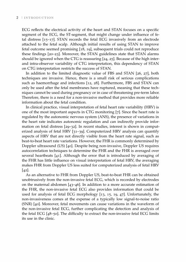
The introduction of cardiotocography (CTG) in the 1960s has enabled contin-uous fetal monitoring [5]. CTG simultaneously records the fetal heart rate (FHR)and uterine activity (UA). CTG allows clinicians to evaluate the fetal responseto the stress caused by uterine contractions and it is currently the main sourceof information to assess fetal distress [6, 7]. In Fig. 1.1, an example is shown ofa CTG recording. Although CTG is the current standard for fetal monitoring, itsdiagnostic value is limited [8, 9]. CTG patterns are interpreted visually, but theinter- and intra-observer variability of CTG interpretation is high [10]. Moreover,the specificity of CTG interpretation is low and the introduction of the CTGhas led to an increase in the rate of unnecessary operative deliveries, withoutimprovement in fetal outcome [7, 9].
There are several diagnostic tools complementary to CTG that clinicians canuse during labor [11]. The most important include fetal blood sampling (FBS)[12] and continuous analysis of the fetal electrocardiogram (ECG) [13, 14]. InFBS, a small droplet of fetal blood is obtained and analyzed to acquire informa-tion about the fetal acid-base balance, which is related to the oxygen concentra-tion in the fetal blood. However, FBS only provides instantaneous informationand requires repeated measurements if the CTG remains abnormal. Besides theinstantaneous information of FBS, continuous analysis of the fetal ECG wave-form is provided by the STAN® (Neoventa Medical, Mölndal, Sweden). The
[ March 26, 2018 at 22:26 – classicthesis version 4.2 ]
2 introduction
ECG reflects the electrical activity of the heart and STAN focuses on a specificsegment of the ECG, the ST-segment, that might change under influence of fe-tal distress [15–17]. STAN records the fetal ECG invasively from an electrodeattached to the fetal scalp. Although initial results of using STAN to improvefetal outcome seemed promising [18, 19], subsequent trials could not reproducethese findings [20–23]. Moreover, the STAN guidelines state that STAN alarmsshould be ignored when the CTG is reassuring [24, 25]. Because of the high inter-and intra-observer variability of CTG interpretation, this dependency of STANon CTG interpretation restricts the success of STAN.
In addition to the limited diagnostic value of FBS and STAN [26, 27], bothtechniques are invasive. Hence, there is a small risk of serious complicationssuch as haemorrhage and infections [12, 28]. Furthermore, FBS and STAN canonly be used after the fetal membranes have ruptured, meaning that these tech-niques cannot be used during pregnancy or in case of threatening pre-term labor.Therefore, there is a need for a non-invasive method that provides more reliableinformation about the fetal condition.
In clinical practice, visual interpretation of fetal heart rate variability (HRV) isone of the most important aspects in CTG monitoring [7]. Since the heart rate isregulated by the autonomic nervous system (ANS), the presence of variations inthe heart rate indicates autonomic regulation and can indirectly provide infor-mation on fetal distress [29–32]. In recent studies, interest is shown in comput-erized analysis of fetal HRV [31–39]. Computerized HRV analysis can quantifyaspects of HRV that are not directly visible from the heart rate signal, such asbeat-to-beat heart rate variations. However, the FHR is commonly determined byDoppler ultrasound (US) [40]. Despite being non-invasive, Doppler US requiresautocorrelation techniques to determine the FHR and the FHR is averaged overseveral heartbeats [41]. Although the error that is introduced by averaging ofthe FHR has little influence on visual interpretation of fetal HRV, the averagingmakes FHR from Doppler US less suited for computerized analysis of fetal HRV[42].
As an alternative to FHR from Doppler US, beat-to-beat FHR can be obtainedunobtrusively from the non-invasive fetal ECG, which is recorded by electrodeson the maternal abdomen [43–46]. In addition to a more accurate estimation ofthe FHR, the non-invasive fetal ECG also provides information that could beused for analysis of fetal ECG morphology [13, 15, 19, 47]. Unfortunately, thenon-invasiveness comes at the expense of a typically low signal-to-noise ratio(SNR) [40]. Moreover, fetal movements can cause variations in the waveform ofthe non-invasive fetal ECG, further complicating the detection and analysis ofthe fetal ECG [48–50]. The difficulty to extract the non-invasive fetal ECG limitsits use in the clinic.
[ March 26, 2018 at 22:26 – classicthesis version 4.2 ]
1.2 goals of this thesis 3
Figure 1.1: Example of a CTG. The FHR and UA are shown in the upper and lower line,respectively.
1.2 Goals of this thesisFrom the previous section it becomes clear that computerized analysis of fetalHRV has great promise as an additional diagnostic tool to assess the fetal con-dition. However, its application in clinical practice is hampered by the fact thatno beat-to-beat FHR is currently available throughout the pregnancy, or is unre-liable due to difficulties to extract the beat-to-beat FHR unobtrusively. Besides,most HRV features that have been presented in the literature are validated foradults in controlled experiments only. For the fetus it is not possible to controlexternal conditions. In particular during labor, uterine contractions can stronglyinfluence the fetal cardiovascular system and thus fetal HRV [1, 51, 52].
Several developments are required before fetal HRV can be used in clinicalpractice. The accomplishment of some of these developments is addressed in thisthesis and explained in two distinctive parts: I) development of new processingtechniques that enable reliable extraction of beat-to-beat FHR from non-invasivefetal ECG recordings and II) the use of fetal HRV analysis for the detection offetal distress during labor.
1.3 Thesis outlineThe physiological and technical background on fetal monitoring that is relevantfor this thesis is provided in Chapter 2. After the background, the first part of thisthesis deals with the signal processing steps that have been developed for reliableFHR detection from non-invasive fetal ECG recordings. In Chapter 3, a newmethod is provided for suppression of the power line interference (PLI). Filteringof the PLI can be seen as a pre-processing step that is required before FHRdetection and analysis of fetal ECG morphology can be performed. To preventdistortion of the fetal ECG waveform, a Kalman smoother with adaptive noiseestimation has been developed.
[ March 26, 2018 at 22:26 – classicthesis version 4.2 ]
4 introduction
Chapter 4 presents a method for FHR detection in non-invasive fetal ECGrecordings. The FHR detection uses predictive models for FHR, fetal ECG mor-phology, and interferences. The models are integrated within a hierarchicalBayesian framework to account for the non-stationary nature of non-invasivefetal ECG recordings. Moreover, we have extended this framework to a multi-channel approach, because the non-invasive fetal ECG is typically recorded us-ing multiple electrodes.
The second part of this thesis addresses some of the challenges related to anal-ysis of fetal HRV. During labor, uterine contractions influence the fetal cardio-vascular system, which results in non-stationarities in the fetal HRV. In Chapter5 we show that separating contractions from rest periods increases the diagnos-tic value of fetal HRV features for the detection of fetal distress during labor.Then, in Chapter 6 we use classification algorithms to show that the detectionrate of fetal distress based on HRV analysis can indeed be improved by combin-ing information from HRV features that are calculated without distinguishingcontractions and information from contraction-dependent HRV features.
Besides influence of uterine contractions, fetal HRV is also influenced by matu-ration of the ANS and several types of medication. Using non-invasive fetal ECGrecordings, we examined the effect of gestational age on fetal HRV in Chapter 7.The effect of corticosteroids, medication that is often used in case of threateningpreterm labor, on fetal HRV is examined in Chapter 8.
The main findings of this thesis are summarized in Chapter 9. This chapter alsoincludes a discussion on promising future research directions. Note that Chap-ters 3-8 are either published or submitted for publication. Each of these chaptersis written to be self-contained, causing some overlap between these chapters.
1.4 List of publications
Journal papers
jp-1 Warmerdam G.J.J., Vullings R., Schmitt L., Van Laar J.O.E.H., and BergmansJ.W.M., Hierarchical Bayesian framework for fetal R-peak detection, usingECG waveform and heart rate information. Submitted.
jp-2 Hulsenboom A.D.J., Warmerdam, G.J.J., Weijers J., Van Laar J.O.E.H., OeiS.G., Blijham P.J., Vullings R., Delhaas T., The effect of head orientation andelectrode placement on ECG waveform in underwater ECG measurement.Submitted.
jp-3 Lempersz C., Van Laar J.O.E.H., Clur S.B., Verdurmen K.M.J., WarmerdamG.J.J., Van der Post J., Blom N.A., Delhaas T., Oei S.G., Vullings R., Thestandardized Fetal Electrocardiogram and its potential use in the detectionof Fetal Congenital Heart disease. Submitted.
[ March 26, 2018 at 22:26 – classicthesis version 4.2 ]

1.4 list of publications 5
jp-4 Warmerdam, G.J.J., Vullings R., Van Laar J.O.E.H., Van der Hout-Van derJagt B., Bergmans J.W.M., Schmitt L., Oei S.G., Detection rate of fetal dis-tress using contraction-dependent fetal heart rate variability analysis. Ac-cepted for publication in Phys. Meas.
jp-5 Verdurmen K.M.J., Warmerdam G.J.J., Lempersz C., Hulsenboom A.D.J.,Renckens J., Dieleman J., Vullings R., Van Laar J.O.E.H., Oei S.G., The in-fluence of betamethasone on fetal heart rate variability, obtained by non-invasive fetal electrocardiogram recordings. Accepted for publication in EarlyHum. Dev.
jp-6 Warmerdam G.J.J., Vullings R., Schmitt L., Van Laar J.O.E.H., and BergmansJ.W.M., A fixed-lag Kalman smoother to filter power line interference inelectrocardiogram recordings. IEEE. Trans. Biomed. Eng. 2017, 64(8): 1852-1861.
jp-7 Warmerdam G.J.J., Vullings R., Van Laar J.O.E.H., Van der Hout-Van derJagt M.B., Bergmans J.W.M., Schmitt L., Oei S.G., Using uterine activityto improve fetal heart rate variability analysis for detection of asphyxiaduring labor. Phys. Meas. 2016, 37: 387-400.
jp-8 Van Laar J.O.E.H., Warmerdam G.J.J., Verdurmen K.M.J., Vullings R., Pe-ters C.H.L., Houterman S., Wijn P.F.F., Andriessen P., Van Pul C., OeiS.G., Fetal heart rate variability in frequency-domain during pregnancy,obtained from noninvasive electrocardiogram recordings. Acta Obstet Gy-necol Scand. 2014, 93: 93-101.
Conference proceedings
cp-1 Verdurmen K.M.J., Warmerdam G.J.J., Lempersz C., Hulsenboom A.D.J.,Renckens J., Dieleman J.P., Vullings R., Van Laar J.O.E.H., Oei S.G., Theinfluence of betamethasone of fetal heart rate variability, obtained by non-invasive fetal electrocardiogram recordings. European Congress on Intra-partum Care, 25-27 May 20017,Stockholm, Sweden.
cp-2 Warmerdam G.J.J., Vullings R., Van Laar J.O.E.H, Bergmans J.W.M., SchmittL., Hierarchical Bayesian framework for fetal R-peak detection using QRSwaveform and heart rate information. Biomedica, 9-10 May 2017, Eind-hoven, The Netherlands.
cp-3 Warmerdam G.J.J., Vullings R., Van Laar J.O.E.H., Van der Hout M.B.,Bergmans J.W.M., Schmitt L., Oei S.G., Selective heart rate variability anal-ysis to account for uterine activity during labor and improve classificationof fetal distress. 38th Annual International Conference of the IEEE EMBS,16-20 August 2016, Orlando, Florida.
[ March 26, 2018 at 22:26 – classicthesis version 4.2 ]

6 introduction
cp-4 Warmerdam G.J.J., Vullings R., Van Laar J.O.E.H., Van der Hout M.B.,Bergmans J.W.M., Schmitt L., Oei S.G., Fetal heart rate variability analysisfor detection of asphyxia can be improved by including uterine activity in-formation. 14th National Day on Biomedical Engineering, 26-27 November2015, Brussels, Belgium.
cp-5 Warmerdam G.J.J., Vullings R., Bergmans J.W.M., Oei S.G., Estimating theerror in spectral analysis of fetal heart rate variability. 5th Dutch Biomed-ical Engineering Conference, 22-23 January 2015, Egmond aan Zee, TheNetherlands.
cp-6 Warmerdam G.J.J., Vullings R., Bergmans J.W.M., Oei S.G., Reliability ofspectral analysis of fetal heart rate variability. 36th Annual InternationalConference of the IEEE EMBS, 26-30 August 2014, Chicago, Illinois.
cp-7 Verdurmen K.M.J., Van Laar J.O.E.H., Warmerdam G.J.J., Oei S.G., Fetalheart rate variability during pregnancy. European Congress of PerinatalMedicine, 4-7 June 2014, Florence, Italy.
cp-8 Warmerdam G.J.J., Vullings, R., Oei, S.G., Wijn, P.F.F., Automated detec-tion of premature atrial contractions in non-invasive fetal electrocardio-gram recordings: a case report. Meeting Abstract: The 3rd InternationalCongress on Cardiac Problems in Pregnancy, 20-23 February 2014, Venice,Italy.
cp-9 Warmerdam G.J.J., Vullings R., Van Laar J.O.E.H., Van der Hout-Van derJagt B., Bergmans J.W.M., Schmitt L., Oei S.G., Accounting for uterine ac-tivity improves fetal heart rate variability analysis for detection of fetaldistress. IEEE SBE Symposium Advancing Healthcare, 18 February 2014,Eindhoven, The Netherlands.
cp-10 Warmerdam G.J.J., Vullings R., Van Pul C., Andriessen P., Oei S.G., WijnP.F.F., QRS classification and spatial combination for robust heart rate de-tection in low-quality fetal ECG recordings. 35th Annual International Con-ference of the IEEE EMBS, 03-07 July 2013, Osaka, Japan.
cp-11 Verdurmen K.M.J., Van Laar J.O.E.H., Warmerdam G.J.J., Oei S.G., Fetalheart rate variability during pregnancy. Symposium on Advances in Peri-natal Monitoring, 24 April 2013, Eindhoven, The Netherlands.
[ March 26, 2018 at 22:26 – classicthesis version 4.2 ]
2 B A C K G R O U N D
2.1 Physiology of the fetal heart
2.1.1 Contraction of the heart
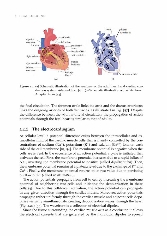
The main function of the heart is to provide vital organs and peripheral tissuewith blood. The adult heart consists of two separate pumps: the right side of theheart pumps oxygen-depleted blood through the lungs (pulmonary circulation)and the left side of the heart pumps oxygenated blood through the peripheralorgans (systemic circulation) (Fig. 2.1a) [53]. Each side of the heart consists oftwo chambers to regulate blood flow into the heart (the atria) and outflow fromthe heart to the pulmonary or systemic circulation (the ventricles).
The contraction of the cardiac muscle originates from the conversion of elec-trical impulses (action potentials) into mechanical activity of the cardiac musclecells [53, 54]. A specialized nervous system conducts the action potentials rapidlythroughout the muscular layer of the heart (the myocardium, Fig. 2.1a). The ac-tion potentials that cause cardiac contraction are generated by self-excitation.Since pacemaker cells located in the sinoatrial (SA) node have the highest self-excitation rate, these cells determine the heart rate. From the SA node, the actionpotentials first propagate through the atria, causing contraction of the atria. Theaction potentials cannot directly cross from the atria to the ventricles. First, theaction potentials need to propagate through the atrioventricular (AV) node andthe bundle of His. After the bundle of His, the nerve fibers split into the left andright bundle branches that end in the left and right ventricles respectively.
When this system functions normally, a delay in propagation is caused by theAV node and the bundle of His, and the atria contract before the ventricularcontraction [53]. This allows the atria to empty their content into the ventriclesand ensures that the ventricles are filled before they pump the blood into thepulmonary and systemic circulation. Another purpose of this system is that itallows all parts of the ventricles to contract simultaneously, optimizing the effec-tive pressure generated by the ventricles [53].
The fetal circulation differs from the adult circulation because the oxygen in-take and the carbon-dioxide secretion take place in the placenta instead of thelungs [55–57]. In the fetal circulation, the right ventricle does not pump theblood through the pulmonary circulation alone. Instead, both ventricles pumpblood through the entire body [57]. To enable this, two interconnections exists in
[ March 26, 2018 at 22:26 – classicthesis version 4.2 ]
8 background
(a) (b)
Figure 2.1: (a) Schematic illustration of the anatomy of the adult heart and cardiac con-duction system. Adapted from [58]. (b) Schematic illustration of the fetal heart.Adapted from [53].
the fetal circulation. The foramen ovale links the atria and the ductus arteriosuslinks the outgoing arteries of both ventricles, as illustrated in Fig. [57]. Despitethe difference between the adult and fetal circulation, the propagation of actionpotentials through the fetal heart is similar to that of adults.
2.1.2 The electrocardiogram
At cellular level, a potential difference exists between the intracellular and ex-tracellular fluid of the cardiac muscle cells that is mainly controlled by the con-centrations of sodium (Na+), potassium (K+) and calcium (Ca2+) ions on eachside of the cell membrane [53, 54]. The membrane potential is negative when thecells are in rest. In the occurrence of an action potential, a cycle is initiated thatactivates the cell. First, the membrane potential increases due to a rapid influx ofNa+, inverting the membrane potential to positive (called depolarization). Then,the membrane potential remains at a plateau level due to the exchange of K+ andCa2+. Finally, the membrane potential returns to its rest value due to persistingoutflow of K+ (called repolarization).
The action potentials propagate from cell to cell by increasing the membranepotential of neighboring rest cells and initiating the depolarization in thesecells[54]. Due to this cell-to-cell activation, the action potential can propagatein any given direction through the cardiac muscle. Moreover, action potentialspropagate rather uniformly through the cardiac muscle and adjacent cells depo-larize virtually simultaneously, creating depolarization waves through the heart(Fig. 2.2a) [53]. The wavefront is a collection of electrical dipoles.
Since the tissue surrounding the cardiac muscle acts as a conductor, it allowsthe electrical currents that are generated by the individual dipoles to spread
[ March 26, 2018 at 22:26 – classicthesis version 4.2 ]
2.1 physiology of the fetal heart 9
(a) (b)
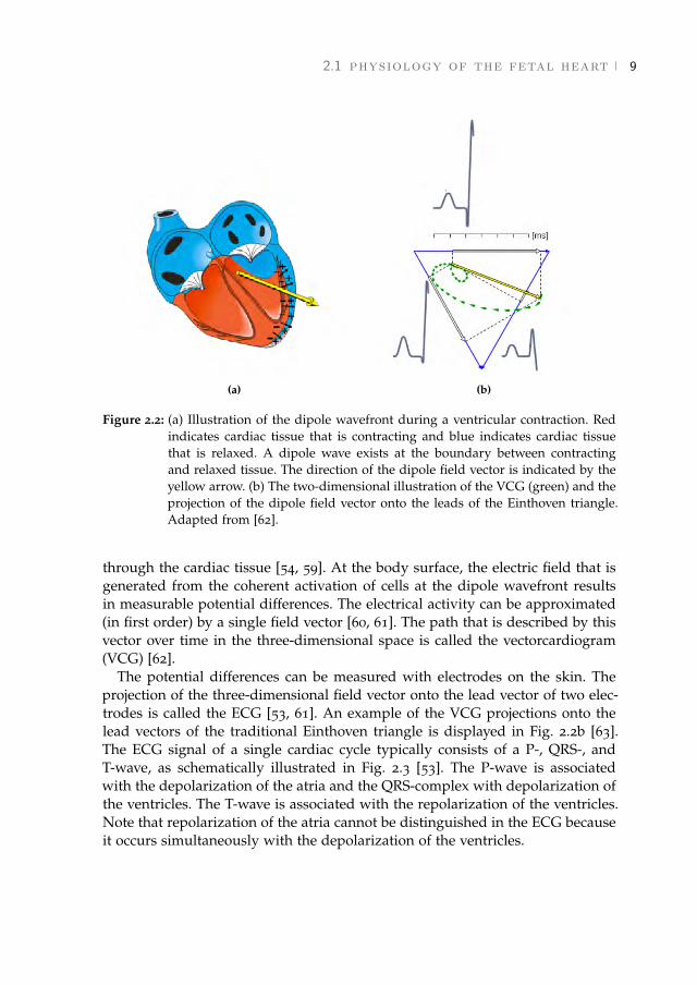
Figure 2.2: (a) Illustration of the dipole wavefront during a ventricular contraction. Redindicates cardiac tissue that is contracting and blue indicates cardiac tissuethat is relaxed. A dipole wave exists at the boundary between contractingand relaxed tissue. The direction of the dipole field vector is indicated by theyellow arrow. (b) The two-dimensional illustration of the VCG (green) and theprojection of the dipole field vector onto the leads of the Einthoven triangle.Adapted from [62].
through the cardiac tissue [54, 59]. At the body surface, the electric field that isgenerated from the coherent activation of cells at the dipole wavefront resultsin measurable potential differences. The electrical activity can be approximated(in first order) by a single field vector [60, 61]. The path that is described by thisvector over time in the three-dimensional space is called the vectorcardiogram(VCG) [62].
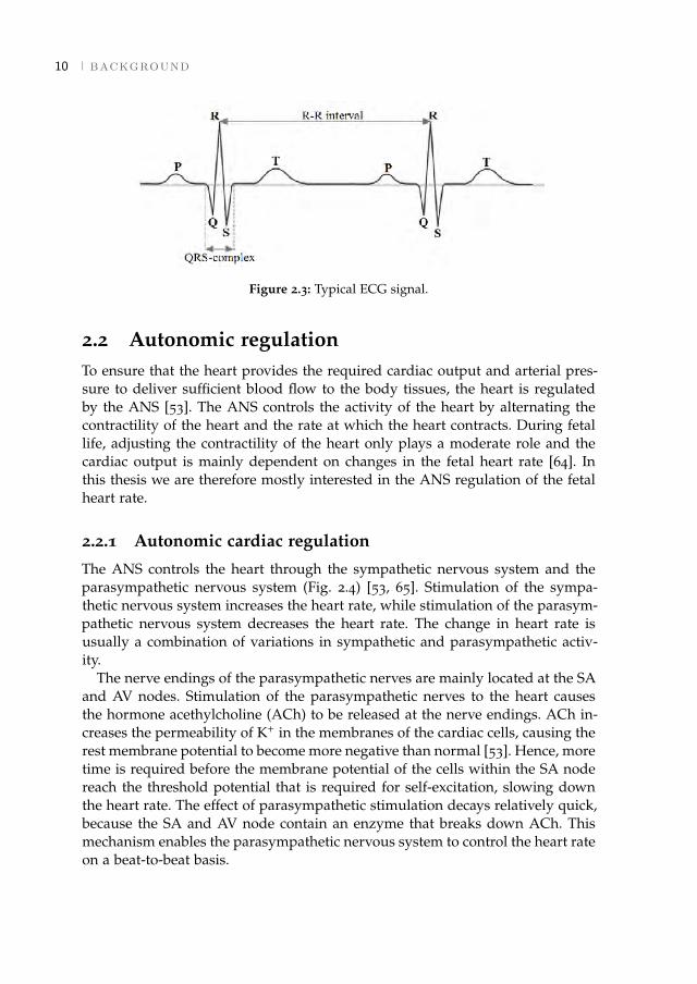
The potential differences can be measured with electrodes on the skin. Theprojection of the three-dimensional field vector onto the lead vector of two elec-trodes is called the ECG [53, 61]. An example of the VCG projections onto thelead vectors of the traditional Einthoven triangle is displayed in Fig. 2.2b [63].The ECG signal of a single cardiac cycle typically consists of a P-, QRS-, andT-wave, as schematically illustrated in Fig. 2.3 [53]. The P-wave is associatedwith the depolarization of the atria and the QRS-complex with depolarization ofthe ventricles. The T-wave is associated with the repolarization of the ventricles.Note that repolarization of the atria cannot be distinguished in the ECG becauseit occurs simultaneously with the depolarization of the ventricles.
[ March 26, 2018 at 22:26 – classicthesis version 4.2 ]
10 background
Figure 2.3: Typical ECG signal.
2.2 Autonomic regulationTo ensure that the heart provides the required cardiac output and arterial pres-sure to deliver sufficient blood flow to the body tissues, the heart is regulatedby the ANS [53]. The ANS controls the activity of the heart by alternating thecontractility of the heart and the rate at which the heart contracts. During fetallife, adjusting the contractility of the heart only plays a moderate role and thecardiac output is mainly dependent on changes in the fetal heart rate [64]. Inthis thesis we are therefore mostly interested in the ANS regulation of the fetalheart rate.
2.2.1 Autonomic cardiac regulation
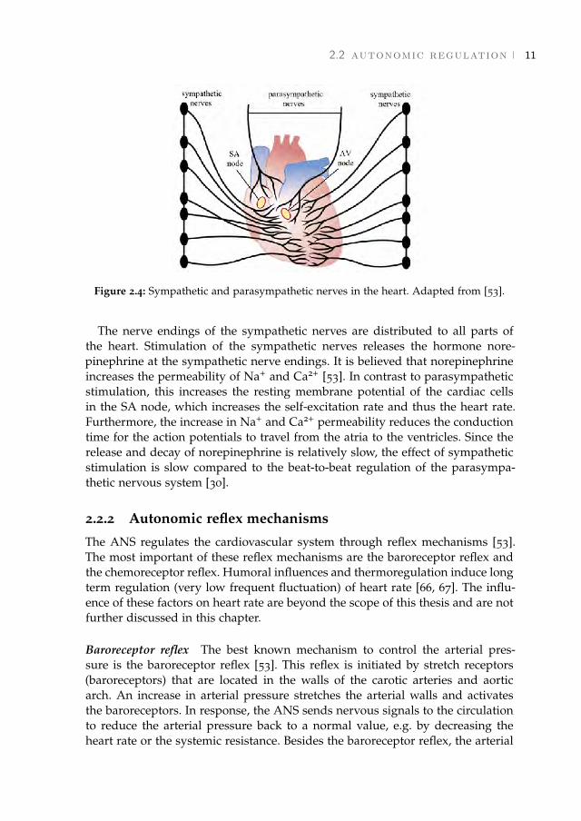
The ANS controls the heart through the sympathetic nervous system and theparasympathetic nervous system (Fig. 2.4) [53, 65]. Stimulation of the sympa-thetic nervous system increases the heart rate, while stimulation of the parasym-pathetic nervous system decreases the heart rate. The change in heart rate isusually a combination of variations in sympathetic and parasympathetic activ-ity.
The nerve endings of the parasympathetic nerves are mainly located at the SAand AV nodes. Stimulation of the parasympathetic nerves to the heart causesthe hormone acethylcholine (ACh) to be released at the nerve endings. ACh in-creases the permeability of K+ in the membranes of the cardiac cells, causing therest membrane potential to become more negative than normal [53]. Hence, moretime is required before the membrane potential of the cells within the SA nodereach the threshold potential that is required for self-excitation, slowing downthe heart rate. The effect of parasympathetic stimulation decays relatively quick,because the SA and AV node contain an enzyme that breaks down ACh. Thismechanism enables the parasympathetic nervous system to control the heart rateon a beat-to-beat basis.
[ March 26, 2018 at 22:26 – classicthesis version 4.2 ]
2.2 autonomic regulation 11
Figure 2.4: Sympathetic and parasympathetic nerves in the heart. Adapted from [53].
The nerve endings of the sympathetic nerves are distributed to all parts ofthe heart. Stimulation of the sympathetic nerves releases the hormone nore-pinephrine at the sympathetic nerve endings. It is believed that norepinephrineincreases the permeability of Na+ and Ca2+ [53]. In contrast to parasympatheticstimulation, this increases the resting membrane potential of the cardiac cellsin the SA node, which increases the self-excitation rate and thus the heart rate.Furthermore, the increase in Na+ and Ca2+ permeability reduces the conductiontime for the action potentials to travel from the atria to the ventricles. Since therelease and decay of norepinephrine is relatively slow, the effect of sympatheticstimulation is slow compared to the beat-to-beat regulation of the parasympa-thetic nervous system [30].
2.2.2 Autonomic reflex mechanisms
The ANS regulates the cardiovascular system through reflex mechanisms [53].The most important of these reflex mechanisms are the baroreceptor reflex andthe chemoreceptor reflex. Humoral influences and thermoregulation induce longterm regulation (very low frequent fluctuation) of heart rate [66, 67]. The influ-ence of these factors on heart rate are beyond the scope of this thesis and are notfurther discussed in this chapter.
Baroreceptor reflex The best known mechanism to control the arterial pres-sure is the baroreceptor reflex [53]. This reflex is initiated by stretch receptors(baroreceptors) that are located in the walls of the carotic arteries and aorticarch. An increase in arterial pressure stretches the arterial walls and activatesthe baroreceptors. In response, the ANS sends nervous signals to the circulationto reduce the arterial pressure back to a normal value, e.g. by decreasing theheart rate or the systemic resistance. Besides the baroreceptor reflex, the arterial
[ March 26, 2018 at 22:26 – classicthesis version 4.2 ]
12 background
pressure is regulated by several interrelated reflex mechanisms (e.g. Brainbridgereflex or respiratory sinus arrhythmia). Since these other mechanisms are lesspronounced for the fetus, they are not further discussed.
Chemoreceptor reflex The chemoreceptor reflex regulates the respiratory activ-ity in a similar way as the baroreceptor reflex controls the arterial pressure [53].The chemoreceptor reflex is initiated by chemoreceptors that are located in thecarotid and aortic arteries. The chemoreceptors are activated when the arterialoxygen concentration falls below normal. For adults, activation of the chemore-ceptors leads to an increase in respiration. The fetal response to changes in oxy-gen concentration differs from that of adults (as discussed in Section 2.2.3), be-cause the fetal oxygen supply does not come from the lungs.
2.2.3 Fetal response to oxygen deficiency
In the fetal circulation, the placenta serves as the lungs of the fetus and it allowsoxygen to diffuse from the maternal circulation to the fetal circulation [68]. Thefetus is connected to the placenta through the umbilical cord. Deoxygenatedblood is transported from the fetus to the placenta, while oxygenated bloodflows from the placenta to the fetus. The oxygenated blood then passes the fetalheart, from where the blood is pumped to the rest of the body tissues. Finally,the oxygen is used in the body tissues and cells to produce energy through aprocess called aerobic metabolism.
During labor, uterine contractions can cause a temporal block of oxygen sup-ply to the fetus [1]. Although maternal placental blood flow is normally high,in case of a strong contraction it can occur that the maternal blood flow to theplacenta is reduced. In this case the fetus has to rely on its own oxygen storage.Besides reduced maternal placental blood flow, fetal oxygen supply can also beinterrupted if the umbilical cord is occluded due to an increase in intrauterinepressure that is caused by uterine contractions. For moderate contractions dur-ing the first stage of labor (the stage of cervical dilation), a connective tissue thatsurround the blood vessels in the umbilical cord can protect the cord vessels.However, during the second stage of labor (the stage of active pushing) it canoccur that intrauterine pressure becomes so high that the connective tissue canno longer oppose this pressure and that the umbilical blood flow is blocked.
In the absence of oxygen, aerobic metabolism can be supported by anaer-obic metabolism [53]. During anaerobic metabolism, glucose reserves are uti-lized to produce energy without oxygen. It is important to note that anaerobicmetabolism only produces a fraction of the energy that is produced during nor-mal aerobic metabolism and there is a risk of damaging the tissues. During aer-obic and anaerobic metabolism hydrogen ions are produced as waste product.Normally, these hydrogen ions are buffered by carbon dioxide and haemoglobin[53]. However, in case the fetus has depleted its buffering capacity, the free hy-drogen ions will cause an increase in the acidity of the blood (measured by the
[ March 26, 2018 at 22:26 – classicthesis version 4.2 ]
2.2 autonomic regulation 13
pH of the blood). After birth, the pH is therefore often used as a measure todetermine the severity of the oxygen deficiency that was suffered by the fetus[22, 69].
Throughout pregnancy, the fetus develops mechanisms that protect it againstoxygen deficiency. These mechanisms, amongst others, involve activation of thebaroreceptor reflex and chemoreceptor reflex [70]. If the umbilical cord is oc-cluded, this will initially increase the systemic resistance in the fetal cardiovas-cular system, causing an increase in fetal blood pressure and activation of thebaroreceptor reflex. Besides, the oxygen concentration in the fetal blood willalso decrease because the fetal oxygen supply is blocked, which activates thechemoreceptors.
There are three stages of oxygen deficiency that can be distinguished [1]. Dur-ing the initial stage of oxygen deficiency, called hypoxemia, the oxygen concen-tration is only decreased in the arterial blood and not in the body tissues. Inresponse, fetal activity is reduced while oxygen uptake in the placenta is op-timized. As the oxygen concentration further decreases, the fetus ensures thatthe oxygen concentration in the central organs (the heart, brain, and adrenals)remains in tact by reducing the blood flow to the peripheral tissues [71, 72]. Thisstage is called hypoxia, in which low oxygen concentration requires anaerobicmetabolism in the peripheral tissues, possibly damaging the peripheral tissue[73]. Because the central organs are protected during hypoxia, the effect on fe-tal outcome is limited. For even lower levels of oxygen concentration, anaerobicmetabolism may also occur in the central organs, which is referred to asphyxia,and there is a risk of damaging the central organs [2]. The ability of the fetusto respond to oxygen deficiency strongly depends on the development of theprotective mechanisms. If these mechanisms have already been used or have notbeen fully developed (i.e. due to prematurity), the oxygen deficiency can lead tofetal morbidity and mortality [74–76].
2.2.4 Fetal autonomic development
The control of FHR by the fetal ANS changes throughout the pregnancy due tomaturation of the fetal ANS [77–79]. Early in the pregnancy, the heart has notyet been fully developed and the heart is autoregulated [80, 81]. Sheep studieshave shown that the sympathetic nervous system becomes functional prior tothe parasympathetic nervous system and dominates the cardiovascular control[82, 83].
Besides maturation of the ANS and fetal heart, also the fetal activity changes asthe fetus develops. Where in the first trimester fetal body movements occur ran-domly over time, in the second half of the pregnancy these movements becomeclustered in rest-activity cycles [84–86]. These rest-activity episodes eventuallyresult in behavioral states that are associated with fetal heart rate patterns andeye movements. Four behavioral states can be distinguished [87]. The first state(1F) is called quiet sleep and little fetal movement occurs. During this stage, the
[ March 26, 2018 at 22:26 – classicthesis version 4.2 ]

14 background
fetal heart rate is stable and changes in the fetal heart rate are relatively small.The second state (2F) is active sleep (or REM-sleep), in which repeated bodymovements and continuous eye movements can be observed. During 2F, largechanges in fetal heart rate can been seen. The final two states are quiet awakeand active awake. These states are of lesser importance since they occur lessfrequently [85, 88].
2.3 Heart rate variabilityComputerized analysis of HRV aims to quantify the functional state of the au-tonomic cardiovascular regulation [30]. Already in the seventies, studies foundthat reduced HRV is associated with an increased risk of mortality after myocar-dial infarction [89]. Since then, the use of HRV analysis expanded from cardiacapplications [90, 91] to a diversity of other pathological conditions, includingneurological disorders such as diabetes [92, 93]. Recently, several studies haveused computerized analysis of fetal HRV to predict fetal distress [31, 32, 34–39].
From Sections 2.1 and 2.2 it becomes clear that the cardiovascular system is acomplex system and the heart rate is only one of the variables that the ANS usesto regulate the cardiovascular system. The variety of factors that can influencethe cardiovascular control (e.g. mental load or physical load) makes the heartrate signal difficult to analyze. Moreover, for long recordings, notable changesin the cardiovascular system may have occurred due to internal influences (e.g.hormones) or changes in the exterior environment. Over the years, various HRVfeatures have been developed that quantify different aspects of the cardiovascu-lar control [94, 95]. This section will briefly discuss several of these features. Fora more detailed description of the HRV features that were used in this study thereader is referred to Chapter 5.
HRV analysis is generally based on the RR-interval signals, the sequence ofintervals between successive R-peaks in the ECG (see Fig. 2.3) [30]. It shouldbe noted that, in theory, true HRV would be measured by the interval betweenthe onset of two successive P-waves (P-P interval), because the P-P intervalsare related to rhythms of the SA node that initiate the cardiac cycle. However,the small amplitude of the P-wave makes accurate detection of the P-P intervaldifficult and detection of the RR-interval is more reliable in practice. Fortunately,changes in RR-intervals and PP-intervals are highly similar [96].
The most straightforward measures for HRV analysis are statistical featuresthat are obtained from the RR-intervals directly [30]. These can generally bedivided into two classes of features: features that are derived directly fromthe RR-intervals and those that are derived from the differences between RR-intervals. Features that focus on the overall R-R signal reflect both sympatheticand parasympathetic regulation. Features that are obtained from the differencesbetween RR-intervals are mostly sensitive to beat-to-beat variations and mainlyreflect parasympathetic regulation [97].
[ March 26, 2018 at 22:26 – classicthesis version 4.2 ]
2.4 non-invasive fetal ecg 15
As explained in Section 2.2.2, the heart rate is regulated by the interplay ofseveral feedback mechanisms that each have their own intrinsic delay [53]. Asa consequence of the delays in these feedback mechanisms, periodic variationsare observed in the heart rate that can be related to different regulatory mech-anisms. To quantify these periodicities, spectral analysis of HRV can be used.The frequency bands of this spectral analysis can be chosen to reflect sympa-thetic and parasympathetic activity [29]. As the effect of sympathetic regulationis relatively slow compared to the parasympathetic regulation, low frequency os-cillations are related to both sympathetic and parasympathetic regulation, whilehigh frequency oscillations are related to parasympathetic regulation alone [29].
Often complicated and irregular variations are seen in the heart rate sincethere are many factors that influence the cardiovascular system[95]. These irreg-ular variations are not well explained by spectral analysis. Because the heart rateis one of the main tools for ANS regulation of the cardiovascular system, theoccurrence of irregularities in the heart rate is indicative of healthy autonomicregulation. The irregularity in the heart rate can be quantified by entropy mea-sures [98, 99].
Besides quantifying HRV at a specific time scale (e.g. as is done with spectralanalysis), other HRV features focus on the ability of the ANS to regulate the car-diovascular system on different time scales [100]. For example, diurnal rhythmsdetermine HRV on a daily basis, hormones influence HRV on the scale of hours,while blood pressure is regulated in seconds to minutes. The relation betweenHRV on different time scales can be described by fractal analysis [38, 100].
It should be noted that many HRV features were originally developed for ana-lyzing ideal and theoretical systems. Calculating these features for physiologicaltime series such as the heart rate might not exactly describe the characteristic itwas originally developed for. Yet, the features may still contain clinically relevantinformation.
2.4 Non-invasive fetal ECGIn clinical practice, fetal HRV is evaluated visually from CTG recordings. DopplerUS is currently the most commonly used technique to record the FHR. The FHRis detected making use of the frequency shift (Doppler effect [101]) that is expe-rienced by ultrasonic waves when they are reflected by moving parts of the fetalheart. Although Doppler US is a non-invasive technique to monitor the FHR, it isprone to signal loss as the US beam needs to be focused at the fetal heart. Move-ments of the transducer or fetal movements results in signal loss and requiresmanual repositioning of the transducer. Moreover, Doppler US is an imprecisemethod to determine the FHR and does not provide beat-to-beat FHR informa-tion. Inaccuracies in the detected FHR can occur because ultrasonic waves detectboth movements of the valves and the walls of the fetal heart. Besides, auto-correlation techniques are used to determine the FHR. As a consequence, the
[ March 26, 2018 at 22:26 – classicthesis version 4.2 ]

16 background
(a) (b)
Figure 2.5: (a) Scalp electrode, adapted from [45]. (b) Non-invasive fetal ECG (Photo withpermission from Nemo healthcare.)
FHR from Doppler US is averaged over several heartbeats, limiting its use forcomputerized analysis of fetal HRV [42].
To obtain the FHR on a beat-to-beat basis, the fetal ECG can be used. Anotheradvantage of using the fetal ECG is that additional diagnostic information canbe obtained through the study of ECG morphology [13, 15, 19, 47]. The fetalECG is generally recorded invasively, using an electrode that is screwed into thefetal scalp (Fig. 2.5a) [102]. Despite having a good signal quality, the invasivefetal ECG can only be used after the fetal membranes have ruptured. Moreover,the signal is acquired using only a single differential electrode and the cardiacelectric activity is thus projected onto a single specific lead axis [103]. This meansthat the three dimensional electric field information of the heart is lost and theECG morphology will depend on the orientation of the fetal heart with respectto the electrode lead [104].
To overcome the limitations of the invasive fetal ECG, it is also possible torecord the fetal ECG non-invasively with electrodes on the maternal abdomen(Fig. 2.5b) [43]. In contrast to the invasive scalp ECG, the non-invasive ECG canbe recorded throughout the pregnancy.
Unfortunately, the non-invasiveness comes at the expense of typically lowSNR. Before the fetal heart signal reaches the abdominal skin, the signal hasto propagate through several layers of tissue that attenuate the electrical activity[105]. The larger the distance between the fetal heart and electrode, the morethe fetal ECG will be attenuated. The overall conductivity of the layers of tissueschanges throughout the gestation [106, 107]. In particular the development of thevernix caseosa strongly influences the signal strength [108]. The vernix caseosais a protective layer that surrounds the fetus, develops from about 28 weeks ofgestation, and starts to dissolve from about 32 weeks of gestation [109]. Becausethe vernix caseosa electrically isolates the fetus, it is very difficult the detect thefetal ECG during this period.
[ March 26, 2018 at 22:26 – classicthesis version 4.2 ]
2.4 non-invasive fetal ecg 17
PLI
Maternal ECG
Fetal ECG
EMG EHG
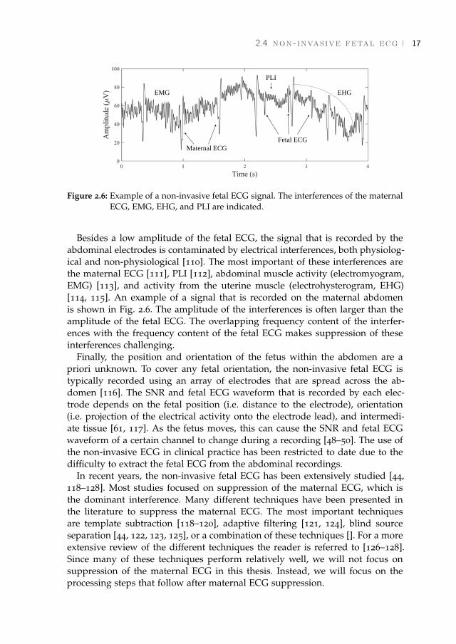
Figure 2.6: Example of a non-invasive fetal ECG signal. The interferences of the maternalECG, EMG, EHG, and PLI are indicated.
Besides a low amplitude of the fetal ECG, the signal that is recorded by theabdominal electrodes is contaminated by electrical interferences, both physiolog-ical and non-physiological [110]. The most important of these interferences arethe maternal ECG [111], PLI [112], abdominal muscle activity (electromyogram,EMG) [113], and activity from the uterine muscle (electrohysterogram, EHG)[114, 115]. An example of a signal that is recorded on the maternal abdomenis shown in Fig. 2.6. The amplitude of the interferences is often larger than theamplitude of the fetal ECG. The overlapping frequency content of the interfer-ences with the frequency content of the fetal ECG makes suppression of theseinterferences challenging.
Finally, the position and orientation of the fetus within the abdomen are apriori unknown. To cover any fetal orientation, the non-invasive fetal ECG istypically recorded using an array of electrodes that are spread across the ab-domen [116]. The SNR and fetal ECG waveform that is recorded by each elec-trode depends on the fetal position (i.e. distance to the electrode), orientation(i.e. projection of the electrical activity onto the electrode lead), and intermedi-ate tissue [61, 117]. As the fetus moves, this can cause the SNR and fetal ECGwaveform of a certain channel to change during a recording [48–50]. The use ofthe non-invasive ECG in clinical practice has been restricted to date due to thedifficulty to extract the fetal ECG from the abdominal recordings.
In recent years, the non-invasive fetal ECG has been extensively studied [44,118–128]. Most studies focused on suppression of the maternal ECG, which isthe dominant interference. Many different techniques have been presented inthe literature to suppress the maternal ECG. The most important techniquesare template subtraction [118–120], adaptive filtering [121, 124], blind sourceseparation [44, 122, 123, 125], or a combination of these techniques []. For a moreextensive review of the different techniques the reader is referred to [126–128].Since many of these techniques perform relatively well, we will not focus onsuppression of the maternal ECG in this thesis. Instead, we will focus on theprocessing steps that follow after maternal ECG suppression.
[ March 26, 2018 at 22:26 – classicthesis version 4.2 ]

[ March 26, 2018 at 22:26 – classicthesis version 4.2 ]

PART I
Analysis of the non-invasive fetalelectrocardiogram
PART I
Analysis of the non-invasive fetalelectrocardiogram
[ March 5, 2018 at 21:28 – classicthesis version 4.2 ]
[ March 26, 2018 at 22:26 – classicthesis version 4.2 ]

[ March 26, 2018 at 22:26 – classicthesis version 4.2 ]
3 A F I X E D - L A G K A L M A N S M O O T H E R T O F I LT E RP O W E R L I N E I N T E R F E R E N C E I N E C GR E C O R D I N G S
Abstract - Objective: Filtering power line interference (PLI) from electrocardiogram(ECG) recordings can lead to significant distortions of the ECG and mask clinicallyrelevant features in ECG waveform morphology. The objective of this study is to filterPLI from ECG recordings with minimal distortion of the ECG waveform. Methods: Inthis paper, we propose a fixed-lag Kalman smoother with adaptive noise estimation. Theperformance of this Kalman smoother in filtering PLI is compared to that of a fixed-bandwidth notch filter and several adaptive PLI filters that have been proposed in theliterature. To evaluate the performance, we corrupted clean neonatal ECG recordingswith various simulated PLI. Furthermore, examples are shown of filtering real PLI froman adult and a fetal ECG recording. Results: The fixed-lag Kalman smoother outperformsother PLI filters in terms of step response settling time (improvements that range from0.1 s to 1 s) and signal-to-noise ratio (improvements that range from 17 dB to 23 dB).Our fixed-lag Kalman smoother can be used for semi real-time applications with a limiteddelay of 0.4 s. Conclusion and significance: The fixed-lag Kalman smoother presentedin this study outperforms other methods for filtering PLI and leads to minimal distortionof the ECG waveform.1
1 This chapter is based on the paper published as Warmerdam G.J.J., Vullings R., Schmitt L., VanLaar J.O.E.H., and Bergmans J.W.M., A fixed-lag Kalman smoother to filter power line interference inelectrocardiogram recordings. IEEE. Trans. Biomed. Eng. 2017, 64(8): 1852-1861.
[ March 26, 2018 at 22:26 – classicthesis version 4.2 ]
22 a kalman smoother to filter power line interference
3.1 IntroductionPower line interference (PLI) is often a source of interference for biomedical sig-nals such as electrocardiogram (ECG) recordings. Electric fields surrounding thepower lines are picked up by the patient, the electric wires, and by the electrocar-diograph itself. Differences in skin-electrode impedance of electrodes can leadto voltage differences measured at the electrodes which are then amplified atthe output. Using a proper recording setup (e.g. cable shielding or amplifierswith a high common mode rejection) can reduce PLI, but this is often insuffi-cient to fully suppress PLI. Especially with developments in sensor technologyin the direction of less obtrusive sensors such as textile electrodes and capaci-tive electrodes [129], PLI can even exceed the ECG in amplitude. Despite thatfiltering PLI is a fairly mature domain [112, 121, 130–136], filtering PLI fromECG recordings remains a challenging task because the frequency content of theECG (in particular the frequency content of the QRS complex) overlaps with thefrequency of the PLI.
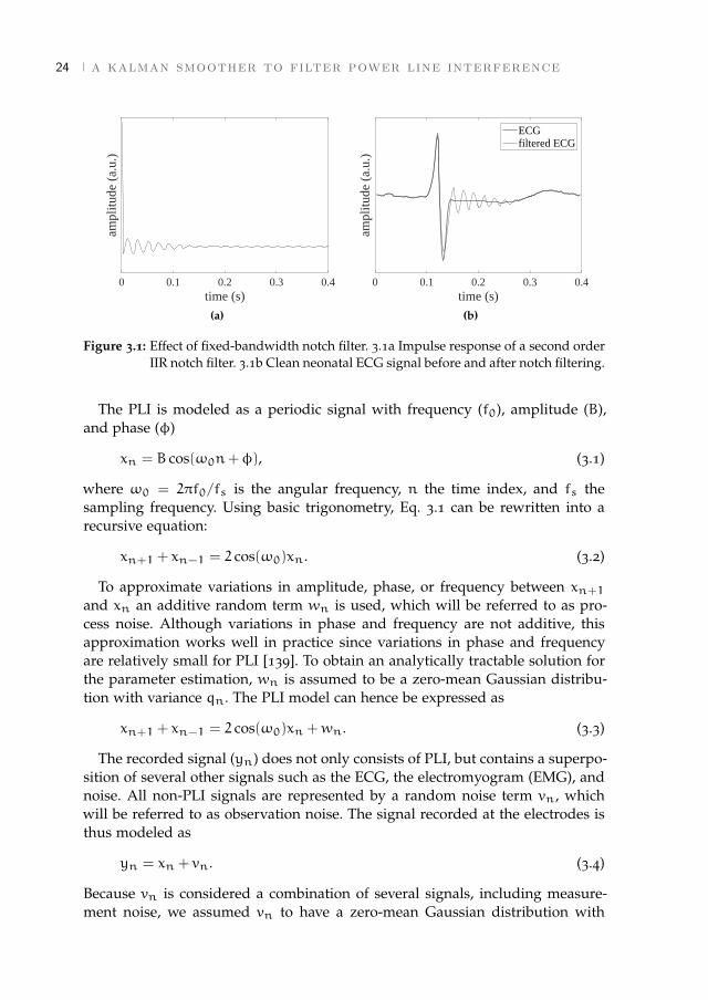
The classical approach for removing PLI is to use a fixed notch filter (e.g.an infinite impulse response (IIR) filter [137]), with unit gain at all frequenciesexcept the PLI frequency. Typically, the impulse response of a notch filter showssome ringing [131], as presented in Fig. 3.1a. In case of a steep QRS complex, thisringing effect is also observed after filtering an ECG signal with the fixed notchfilter. In particular for neonatal and fetal ECG, ringing can lead to significantdisturbance of the ECG, as shown in Fig. 3.1b. The shorter duration of the QRScomplex (typically 50 ms for neonates and 40 ms for fetuses) compared to theduration of the adult QRS complex (typically 80 ms) [138], leads to more overlapof the frequency content of the QRS complex with the frequency of the PLI.Note that since ringing is a response of the notch filter to a QRS complex, usinga notch filter will always cause ringing, even in case there is little to no PLI.
As an alternative to notch filters with fixed parameters, several adaptive fil-ters have been proposed in the literature [112, 121, 132–136]. Least-mean-square(LMS) adaptive algorithms were used in [112, 121, 132–134]. The first adaptivefilters that were developed had the practical limitation that they required an ex-ternally recorded reference signal [121, 132, 133]. In contrast, an algorithm thatrequired no additional reference signal was suggested by Ziarani et al. [134]. In[112], Martens et al. made improvements to the algorithm of Ziarani, resultingin a more stable filter. More recently, some researchers have used a Kalman fil-ter (KF) [135] and extended KF [136] for PLI tracking and cancellation. UnlikeLMS algorithms that use a fixed learning rate, KFs have the advantage that thelearning rate of the filter is adapted to the signal-to-noise ratio (SNR).
Although most of these studies also consider the possibility of frequency de-viations of the PLI, frequency deviations are only of the order ± 0.01 Hz in mostdeveloped countries according to the power system quality standards [139]. Incontrast to the relatively stable frequency, the amplitude and phase of the PLIcan significantly change, e.g. due to different patient positioning or impedance
[ March 26, 2018 at 22:26 – classicthesis version 4.2 ]
3.2 methods 23
changes. A linear KF was suggested by Sameni that combined variations inboth amplitude and phase into the estimation of a single parameter [135]. Thismethod has the advantage that it does not require a priori knowledge of the PLIamplitude and phase dynamics.
One of the main problems with adaptive filtering of PLI from ECG record-ings is the interference of the QRS complex with the parameter estimation [112,133]. While fast adaptation of model parameters is preferred in order to trackchanges in the PLI, using high learning rates will also allow model parametersto adapt to the QRS complex, hence leading to distortion of the ECG waveform.To prevent model parameters from adapting to the QRS complex, several stud-ies have suggested to reduce the learning rate during a QRS complex or evenset the learning rate to zero, either based on R-peak locations [133] or based onsome general properties of the QRS complex [112]. Reducing the learning rateduring a QRS complex has shown promising results. Unfortunately, in case ofa time-varying PLI this approach leads to an error in the estimation of the PLIafter a QRS complex.
In this study we suggest to use a Kalman smoother (KS) to improve estimationof the PLI. A smoother consists of a combination of two filters: one filter oper-ates on past observations (called a forward filter), while the other filter operateson future observations (called a backward filter) [140]. Ideally, the forward andbackward parameter estimation have uncorrelated errors and the combinationof the two improves the parameter estimation [140, 141]. Besides the advantageof improving the parameter estimation, a KS also reduces the error made by theinterference of QRS complexes with the parameter estimation. Because smooth-ing requires future information, a delay is generated in the estimation of the PLI.However, for most real-time applications a small delay is acceptable. We there-fore propose a fixed-lag KS that estimates the PLI for some fixed delay [142].
The rest of this paper is organized as follows; in section 3.2.1 and 3.2.2 thelinear KF and extension to a fixed-lag KS are discussed. Noise estimation thataccounts for the interference of the ECG with the parameter estimation of thePLI is discussed in sections 4.2.1 and 3.2.4. Then section 6.2.1 discusses the dataacquisition and simulation of the PLI that is used to validate the developedmethod. For validation we used neonatal ECG recordings, but the developedalgorithm can equally be applied to adult and fetal ECG recordings, as is shownby two examples. Finally, our work is compared to several other algorithmsproposed in the literature, and results and discussion are presented in sections6.3 and 6.4.
3.2 Methods
3.2.1 Linear Kalman filter
Implementation of the linear KF is based on the work presented by Sameni [135].This section summarizes the main concepts of the KF.
[ March 26, 2018 at 22:26 – classicthesis version 4.2 ]
24 a kalman smoother to filter power line interference
0 0.1 0.2 0.3 0.4time (s)
ampl
itude
(a.
u.)
(a)
0 0.1 0.2 0.3 0.4time (s)
ampl
itude
(a.
u.)
ECGfiltered ECG
(b)
Figure 3.1: Effect of fixed-bandwidth notch filter. 3.1a Impulse response of a second orderIIR notch filter. 3.1b Clean neonatal ECG signal before and after notch filtering.
The PLI is modeled as a periodic signal with frequency (f0), amplitude (B),and phase (φ)
xn = B cos(ω0n+φ), (3.1)
where ω0 = 2πf0/fs is the angular frequency, n the time index, and fs thesampling frequency. Using basic trigonometry, Eq. 3.1 can be rewritten into arecursive equation:
xn+1 + xn−1 = 2 cos(ω0)xn. (3.2)
To approximate variations in amplitude, phase, or frequency between xn+1and xn an additive random term wn is used, which will be referred to as pro-cess noise. Although variations in phase and frequency are not additive, thisapproximation works well in practice since variations in phase and frequencyare relatively small for PLI [139]. To obtain an analytically tractable solution forthe parameter estimation, wn is assumed to be a zero-mean Gaussian distribu-tion with variance qn. The PLI model can hence be expressed as
xn+1 + xn−1 = 2 cos(ω0)xn +wn. (3.3)
The recorded signal (yn) does not only consists of PLI, but contains a superpo-sition of several other signals such as the ECG, the electromyogram (EMG), andnoise. All non-PLI signals are represented by a random noise term vn, whichwill be referred to as observation noise. The signal recorded at the electrodes isthus modeled as
yn = xn + vn. (3.4)
Because vn is considered a combination of several signals, including measure-ment noise, we assumed vn to have a zero-mean Gaussian distribution with
[ March 26, 2018 at 22:26 – classicthesis version 4.2 ]

3.2 methods 25
variance rn. Note that since vn also models the ECG, this assumption is onlyapproximately true. However, in [142] it is shown that even in case of non Gaus-sian noise, a KF is the optimal linear estimator in the sense that it minimizes themean square error.
Based on Eqs. 3.3 and 3.4 we can define a state-space model that describes thePLI as follows:
xn+1 = Axn +bwnyn+1 = hTxn+1 + vn+1,
(3.5)
where xn =
[xnxn−1
], A =
[2cos(ω0) −1
1 0
], b =
[1
0
], and h =
[1
0
].
Given observations yn+1, our aim is to estimate the parameter xn+1. Thefirst element of the estimate of xn+1 is then our estimation of the PLI at timen+ 1. Due to the uncertainties in the state-space model described by Eq. 4.6, aprobabilistic approach can be used to solve the PLI estimation problem. In thiscase we are interested in xn+1 that maximizes the posterior probability densityfunction p(xn+1|yn+1, I), with I = {A,b,h,qn, rn}.
According to Bayes’ rule, we can describe the PLI parameter estimation prob-lem as
p(xn+1|yn+1, I) =p(yn+1|xn+1, I)p(xn+1|yn, I)
p(yn+1|yn, I). (3.6)
Due to the assumption of Gaussian process and measurement noise, the poste-rior is a Gaussian distribution and it is fully described by its mean xn+1|n+1and its associated covariance Pn+1|n+1. The notation xn+1|n+1 represents theestimation of x at time n+ 1, given observations Y = {y1,y2, ...,yn+1}.
Using a similar derivation as described in [143], the maximum a posteriori(MAP) estimate of the PLI xn+1|n+1 and its covariance Pn+1|n+1 can sequen-tially be updated according to the KF equations, given by:
xn+1|n+1 =Axn|n +Kn(yn+1 −hTAxn|n) (3.7)
Pn+1|n+1 =APn|nAT + qnbb
T −KnhT (APn|nA
T + qnbbT ) (3.8)
and Kn the Kalman gain [144]:
Kn =(APn|nA
T + qnbbT )h
hT (APn|nAT + qnbbT )h+ rn+1
. (3.9)
After estimating the PLI, the ECG signal is obtained by the innovation signalof the KF:
vn+1 = yn+1 − xn+1|n+1, (3.10)
where xn+1|n+1 is the first element of xn+1|n+1.
[ March 26, 2018 at 22:26 – classicthesis version 4.2 ]

26 a kalman smoother to filter power line interference
3.2.2 Fixed-lag Kalman Smoother
The KF update equations described by Eqs. 3.7-3.9 provide causal estimationsof the PLI, which means that at time n+ 1 they yield estimates given all pastobservations and the current observation (Y). While for real-time applicationscausality is required, for most applications a small delay of τ samples is often ac-ceptable to improve the estimation accuracy. When appropriately designed, thecombination of a causal filter and a backward filter that uses future informationresults in smaller estimation errors compared to the causal filter alone [140, 141].
Our goal is to estimate xn−τ|n+1 for some fixed time-lag τ. In other words,we want to estimate the state at time n− τ, given past observations {y1, ...,yn−τ}and future observations {yn−τ+1, ...,yn+1}. The key concept is to define an aug-mented state vector xa ∈ R2(τ+1) [142]
xan+1 =
x(0)n+1
x(1)n+1
...x(τ+1)n+1
=
A 0 · · · 0
I2 0 · · · 0
0 I2 · · · 0...
... · · ·...
0 · · · I2 0
x(0)n
x(1)n
...x(τ+1)n
+
b
0...0
wn, (3.11)
with I2 is the [2× 2] identity matrix and element x(i)n+1 is the ith time lag ofxn+1.
From Eq. 3.11, we can see that, except for the first component, the compo-nents of the augmented vector xan+1 are sequentially delayed versions of the
previous augmented vector xan. Moreover, if we initialize x(0)n as the state at timen of the original system described by Eq. 4.6, we observe that the first row ofthe augmented system describes the original system, while the remaining rowsgive successive time delays. The last component of the estimate xa
n+1|n+1 isxn−τ|n+1, which is the estimate we are looking for.
Based on the augmented state vector, we can obtain an augmented state-spacemodel
xan+1 = Aaxan +bawn
yn+1 = haTxan+1 + vn+1,
(3.12)
with model parameters defined as
Aa =
A 0 · · · 0
I2 0 · · · 0
0 I2 · · · 0...
... · · ·...
0 · · · I2 0
, ba =
b
0...0
, and ha =
h
0...0
. (3.13)
[ March 26, 2018 at 22:26 – classicthesis version 4.2 ]
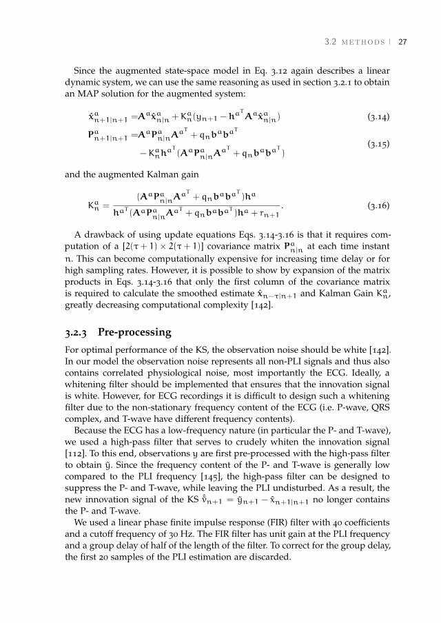
3.2 methods 27
Since the augmented state-space model in Eq. 3.12 again describes a lineardynamic system, we can use the same reasoning as used in section 3.2.1 to obtainan MAP solution for the augmented system:
xan+1|n+1 =Aaxan|n +Kan(yn+1 −haTAaxan|n) (3.14)
Pan+1|n+1 =AaPan|nAaT + qnb
abaT
−KanhaT (AaPan|nA
aT + qnbaba
T)
(3.15)
and the augmented Kalman gain
Kan =(AaPa
n|nAa
T+ qnb
abaT)ha
haT(AaPa
n|nAa
T+ qnbaba
T)ha + rn+1
. (3.16)
A drawback of using update equations Eqs. 3.14-3.16 is that it requires com-putation of a [2(τ + 1)× 2(τ + 1)] covariance matrix Pa
n|nat each time instant
n. This can become computationally expensive for increasing time delay or forhigh sampling rates. However, it is possible to show by expansion of the matrixproducts in Eqs. 3.14-3.16 that only the first column of the covariance matrixis required to calculate the smoothed estimate xn−τ|n+1 and Kalman Gain Kan,greatly decreasing computational complexity [142].
3.2.3 Pre-processing
For optimal performance of the KS, the observation noise should be white [142].In our model the observation noise represents all non-PLI signals and thus alsocontains correlated physiological noise, most importantly the ECG. Ideally, awhitening filter should be implemented that ensures that the innovation signalis white. However, for ECG recordings it is difficult to design such a whiteningfilter due to the non-stationary frequency content of the ECG (i.e. P-wave, QRScomplex, and T-wave have different frequency contents).
Because the ECG has a low-frequency nature (in particular the P- and T-wave),we used a high-pass filter that serves to crudely whiten the innovation signal[112]. To this end, observations y are first pre-processed with the high-pass filterto obtain y. Since the frequency content of the P- and T-wave is generally lowcompared to the PLI frequency [145], the high-pass filter can be designed tosuppress the P- and T-wave, while leaving the PLI undisturbed. As a result, thenew innovation signal of the KS ˆvn+1 = yn+1 − xn+1|n+1 no longer containsthe P- and T-wave.
We used a linear phase finite impulse response (FIR) filter with 40 coefficientsand a cutoff frequency of 30 Hz. The FIR filter has unit gain at the PLI frequencyand a group delay of half of the length of the filter. To correct for the group delay,the first 20 samples of the PLI estimation are discarded.
[ March 26, 2018 at 22:26 – classicthesis version 4.2 ]

28 a kalman smoother to filter power line interference
3.2.4 Noise estimation
Sameni showed that under assumption of stationary observation and processnoise (rn = r and qn = q), the KF described in section 3.2.1 converges to asecond order notch filter [135]. When the amplitude or phase of the PLI varies,or in case of non-stationary observation noise this assumption is incorrect andthe KF performs sub-optimally.
Observation noise
In contrast to the frequency content of the P- and T-wave, the frequency contentof the QRS complex overlaps with the PLI frequency. Therefore, a high-pass filteris not able to fully suppress the QRS complex with respect to the PLI and y stillcontains remainders of the QRS complex. Due to the remainders of the QRScomplex, the variance in the observation noise is time-varying and increasesduring a QRS complex. Moreover, remainders of the QRS complex also cause atemporal increase in the correlation of y. Hence, the innovation signal ˆv will beless white during a QRS complex, reducing the performance of the parameterestimation by the KS.
From Eq. 3.9 we can see that an increase in rn+1 will lead to a decrease inKn. In turn, from Eq. 3.7 we can observe that for low Kn, a new estimation ofthe PLI (xn+1|n+1) will mostly depend on the a priori estimate (Axn|n) and lesson observation yn+1. Therefore, to reduce the influence of the remainders ofthe QRS complex on the parameter estimation, it is important to include in ourmethod a time-varying estimation of rn+1.
Since rn+1 represents the variance of the signal without PLI, it can be esti-mated based on the signal that remains after passing y through a forward coarsefixed-bandwidth notch filter (yf). However, after a sudden change in PLI (e.g. astep increase in amplitude), yf will be contaminated by some remaining PLI dueto the response time of the fixed-bandwidth notch filter, as shown in Fig. 3.2a. Asa consequence, if rn+1 is estimated based on yf, the value of rn+1 will increaseafter a sudden change in PLI. In turn, the increase in rn+1 leads to a decreasein Kn, while actually an increase in Kn is required for fast adaptation of the KSmodel parameters to the changes in PLI.
Instead of estimating rn+1 only based on yf, we estimate rn+1 based on acombination of yf and a backward fixed-bandwidth notch filter (denoted as yb).If a sudden change in PLI occurs at time t, yf has no remaining PLI before timet, while yb has no remaining PLI after time t, as shown in Fig. 3.2a. Combininginformation from yf and yb leads to an accurate estimation of rn+1, except attime t.
By taking the sum of absolute values for yf and yb over a time window M
that corresponds to the length of a QRS complex, the amplitudes of the resulting
[ March 26, 2018 at 22:26 – classicthesis version 4.2 ]

3.2 methods 29
0 0.5 1time (s)
y
yf
yb
(a)
0 0.5 1time (s)
r n (a.
u.)
rf
rb
r
(b)
Figure 3.2: Estimation of the observation noise rn.
signals are expected to be higher during a QRS complex with respect to otherparts of the signals. We thus estimate the observation noise as:
rn =1
M
n+M/2∑j=n−M/2
∣∣yfj ∣∣ · 1Mn+M/2∑j=n−M/2
∣∣ybj ∣∣. (3.17)
As fixed-bandwidth notch filter we use a second-order Butterworth notch filter,with cutoff frequencies of 45 Hz and 55 Hz. Note that the approach describedabove requires a delay τfb to compute yb. Because rn+1 needs to be calculatedin order to obtain the smoothed estimate of the PLI at time n− τ, the delay τfb
is in addition to the delay τ of the fixed-lag KS.
Process noise
As noted by Sameni, the ratio between the observation and process noise (γn =
qn/rn) is related to the quality factor (Q-factor) of the KF described in section3.2.1 [135]. Low γn is related to a high Q-factor and a narrow bandwidth notchfilter. High γn is related to a low Q-factor and a broad bandwidth notch filter.
Similar to [135], an average value γ is chosen and γ is then adjusted to varia-tions in SNR. Variations around γ are based on the ratio between the variance ofthe innovation signal and the estimated variance of the innovation signal by theKS [135]. The value of γn is estimated as
γn = γ ·ˆv2n
hT (APn−1|n−1AT + qn−1bbT )h+ rn
. (3.18)
The process covariance qn can then be estimated as the product of γn and rn.However, as discussed in section 3.2.4 both rn and ˆvn increase during a QRScomplex, due to remainders of the QRS complex in y. This means that the pro-cess noise also increases during a QRS complex, leading to a faster adaptation of
[ March 26, 2018 at 22:26 – classicthesis version 4.2 ]
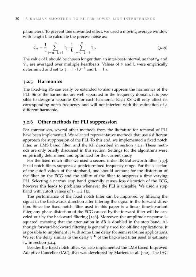
30 a kalman smoother to filter power line interference
parameters. To prevent this unwanted effect, we used a moving average windowwith length L to calculate the process noise as:
qn =1
L
n∑j=n−L+1
rj ·1
L
n∑j=n−L+1
γj. (3.19)
The value of L should be chosen longer than an inter-beat-interval, so that rn andγn are averaged over multiple heartbeats. Values of γ and L were empiricallydetermined and set to γ = 1 · 10−3 and L = 1 s.
3.2.5 Harmonics
The fixed-lag KS can easily be extended to also suppress the harmonics of thePLI. Since the harmonics are well separated in the frequency domain, it is pos-sible to design a separate KS for each harmonic. Each KS will only affect itscorresponding notch frequency and will not interfere with the estimation of adifferent harmonic.
3.2.6 Other methods for PLI suppression
For comparison, several other methods from the literature for removal of PLIhave been implemented. We selected representative methods that use a differentapproach for suppression of the PLI. To this end, we implemented a fixed notchfilter, an LMS based filter, and the KF described in section 3.2.1. These meth-ods are only briefly discussed in this section. Settings for the algorithms wereempirically determined and optimized for the current study.
For the fixed notch filter we used a second order IIR Butterworth filter [137].Fixed notch filters suppress a predetermined frequency range. For the selectionof the cutoff values of the stopband, one should account for the distortion ofthe filter on the ECG and the ability of the filter to suppress a time varyingPLI. Selecting a narrow stop band generally causes less distortion of the ECG,however this leads to problems whenever the PLI is unstable. We used a stopband with cutoff values of f0 ± 2 Hz.
The performance of the fixed notch filter can be improved by filtering thesignal in the backwards direction after filtering the signal in the forward direc-tion. Since the fixed notch filter used in this paper is a linear time-invariantfilter, any phase distortion of the ECG caused by the forward filter will be can-celed out by the backward filtering [146]. Moreover, the amplitude response issquared, meaning that the attenuation in dB is doubled in the stop band. Al-though forward-backward filtering is generally used for off-line applications, itis possible to implement it with some time delay for semi real-time applications.We set the delay similar to the delay τfb of the backward filter used to estimatern in section 3.2.4.
Besides the fixed notch filter, we also implemented the LMS based ImprovedAdaptive Canceller (IAC), that was developed by Martens et al. [112]. The IAC
[ March 26, 2018 at 22:26 – classicthesis version 4.2 ]
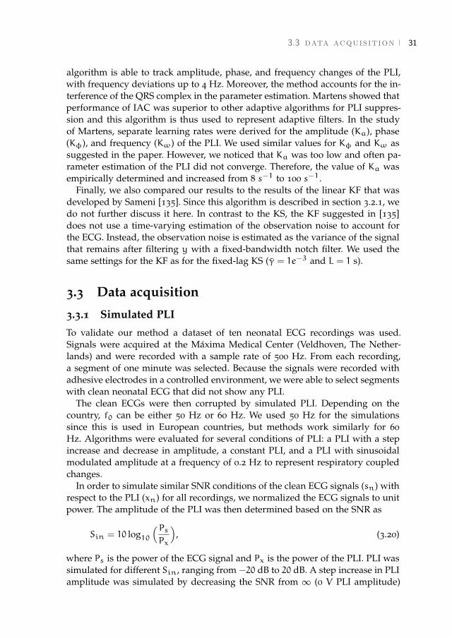
3.3 data acquisition 31
algorithm is able to track amplitude, phase, and frequency changes of the PLI,with frequency deviations up to 4 Hz. Moreover, the method accounts for the in-terference of the QRS complex in the parameter estimation. Martens showed thatperformance of IAC was superior to other adaptive algorithms for PLI suppres-sion and this algorithm is thus used to represent adaptive filters. In the studyof Martens, separate learning rates were derived for the amplitude (Ka), phase(Kφ), and frequency (Kω) of the PLI. We used similar values for Kφ and Kω assuggested in the paper. However, we noticed that Ka was too low and often pa-rameter estimation of the PLI did not converge. Therefore, the value of Ka wasempirically determined and increased from 8 s−1 to 100 s−1.
Finally, we also compared our results to the results of the linear KF that wasdeveloped by Sameni [135]. Since this algorithm is described in section 3.2.1, wedo not further discuss it here. In contrast to the KS, the KF suggested in [135]does not use a time-varying estimation of the observation noise to account forthe ECG. Instead, the observation noise is estimated as the variance of the signalthat remains after filtering y with a fixed-bandwidth notch filter. We used thesame settings for the KF as for the fixed-lag KS (γ = 1e−3 and L = 1 s).
3.3 Data acquisition
3.3.1 Simulated PLI
To validate our method a dataset of ten neonatal ECG recordings was used.Signals were acquired at the Máxima Medical Center (Veldhoven, The Nether-lands) and were recorded with a sample rate of 500 Hz. From each recording,a segment of one minute was selected. Because the signals were recorded withadhesive electrodes in a controlled environment, we were able to select segmentswith clean neonatal ECG that did not show any PLI.
The clean ECGs were then corrupted by simulated PLI. Depending on thecountry, f0 can be either 50 Hz or 60 Hz. We used 50 Hz for the simulationssince this is used in European countries, but methods work similarly for 60Hz. Algorithms were evaluated for several conditions of PLI: a PLI with a stepincrease and decrease in amplitude, a constant PLI, and a PLI with sinusoidalmodulated amplitude at a frequency of 0.2 Hz to represent respiratory coupledchanges.
In order to simulate similar SNR conditions of the clean ECG signals (sn) withrespect to the PLI (xn) for all recordings, we normalized the ECG signals to unitpower. The amplitude of the PLI was then determined based on the SNR as
Sin = 10 log10(PsPx
), (3.20)
where Ps is the power of the ECG signal and Px is the power of the PLI. PLI wassimulated for different Sin, ranging from −20 dB to 20 dB. A step increase in PLIamplitude was simulated by decreasing the SNR from ∞ (0 V PLI amplitude)
[ March 26, 2018 at 22:26 – classicthesis version 4.2 ]
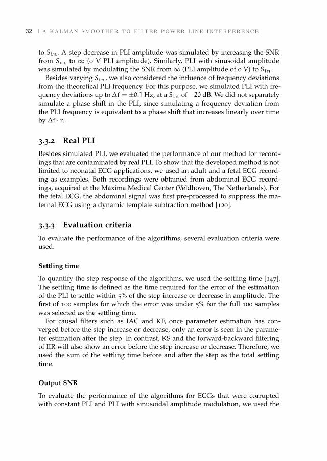
32 a kalman smoother to filter power line interference
to Sin. A step decrease in PLI amplitude was simulated by increasing the SNRfrom Sin to ∞ (0 V PLI amplitude). Similarly, PLI with sinusoidal amplitudewas simulated by modulating the SNR from∞ (PLI amplitude of 0 V) to Sin.
Besides varying Sin, we also considered the influence of frequency deviationsfrom the theoretical PLI frequency. For this purpose, we simulated PLI with fre-quency deviations up to ∆f = ±0.1 Hz, at a Sin of −20 dB. We did not separatelysimulate a phase shift in the PLI, since simulating a frequency deviation fromthe PLI frequency is equivalent to a phase shift that increases linearly over timeby ∆f ·n.
3.3.2 Real PLI
Besides simulated PLI, we evaluated the performance of our method for record-ings that are contaminated by real PLI. To show that the developed method is notlimited to neonatal ECG applications, we used an adult and a fetal ECG record-ing as examples. Both recordings were obtained from abdominal ECG record-ings, acquired at the Máxima Medical Center (Veldhoven, The Netherlands). Forthe fetal ECG, the abdominal signal was first pre-processed to suppress the ma-ternal ECG using a dynamic template subtraction method [120].
3.3.3 Evaluation criteria
To evaluate the performance of the algorithms, several evaluation criteria wereused.
Settling time
To quantify the step response of the algorithms, we used the settling time [147].The settling time is defined as the time required for the error of the estimationof the PLI to settle within 5% of the step increase or decrease in amplitude. Thefirst of 100 samples for which the error was under 5% for the full 100 sampleswas selected as the settling time.
For causal filters such as IAC and KF, once parameter estimation has con-verged before the step increase or decrease, only an error is seen in the parame-ter estimation after the step. In contrast, KS and the forward-backward filteringof IIR will also show an error before the step increase or decrease. Therefore, weused the sum of the settling time before and after the step as the total settlingtime.
Output SNR
To evaluate the performance of the algorithms for ECGs that were corruptedwith constant PLI and PLI with sinusoidal amplitude modulation, we used the
[ March 26, 2018 at 22:26 – classicthesis version 4.2 ]
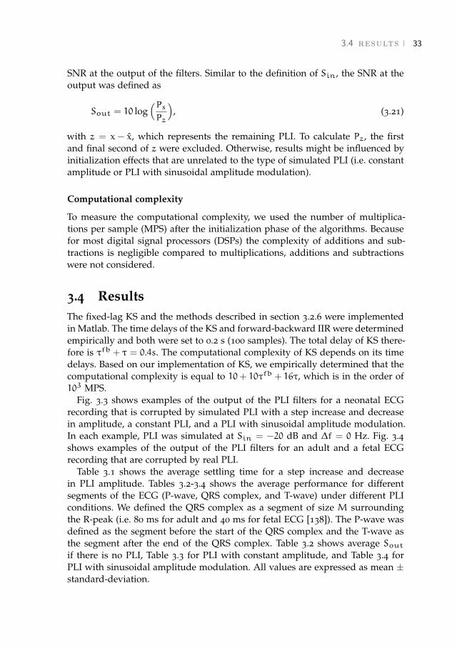
3.4 results 33
SNR at the output of the filters. Similar to the definition of Sin, the SNR at theoutput was defined as
Sout = 10 log(PsPz
), (3.21)
with z = x − x, which represents the remaining PLI. To calculate Pz, the firstand final second of z were excluded. Otherwise, results might be influenced byinitialization effects that are unrelated to the type of simulated PLI (i.e. constantamplitude or PLI with sinusoidal amplitude modulation).
Computational complexity
To measure the computational complexity, we used the number of multiplica-tions per sample (MPS) after the initialization phase of the algorithms. Becausefor most digital signal processors (DSPs) the complexity of additions and sub-tractions is negligible compared to multiplications, additions and subtractionswere not considered.
3.4 ResultsThe fixed-lag KS and the methods described in section 3.2.6 were implementedin Matlab. The time delays of the KS and forward-backward IIR were determinedempirically and both were set to 0.2 s (100 samples). The total delay of KS there-fore is τfb + τ = 0.4s. The computational complexity of KS depends on its timedelays. Based on our implementation of KS, we empirically determined that thecomputational complexity is equal to 10+ 10τfb + 16τ, which is in the order of103 MPS.
Fig. 3.3 shows examples of the output of the PLI filters for a neonatal ECGrecording that is corrupted by simulated PLI with a step increase and decreasein amplitude, a constant PLI, and a PLI with sinusoidal amplitude modulation.In each example, PLI was simulated at Sin = −20 dB and ∆f = 0 Hz. Fig. 3.4shows examples of the output of the PLI filters for an adult and a fetal ECGrecording that are corrupted by real PLI.
Table 3.1 shows the average settling time for a step increase and decreasein PLI amplitude. Tables 3.2-3.4 shows the average performance for differentsegments of the ECG (P-wave, QRS complex, and T-wave) under different PLIconditions. We defined the QRS complex as a segment of size M surroundingthe R-peak (i.e. 80 ms for adult and 40 ms for fetal ECG [138]). The P-wave wasdefined as the segment before the start of the QRS complex and the T-wave asthe segment after the end of the QRS complex. Table 3.2 shows average Soutif there is no PLI, Table 3.3 for PLI with constant amplitude, and Table 3.4 forPLI with sinusoidal amplitude modulation. All values are expressed as mean ±standard-deviation.
[ March 26, 2018 at 22:26 – classicthesis version 4.2 ]

34 a kalman smoother to filter power line interference
0 0.5 1 1.5time (s)
KS
KF
IAC
IIR
y
ECG
(a) Step increase.
0 0.5 1 1.5time (s)
KS
KF
IAC
IIR
y
ECG
(b) Step decrease.
0 0.5 1 1.5time (s)
KS
KF
IAC
IIR
y
ECG
(c) Constant amplitude.
0 0.5 1 1.5time (s)
KS
KF
IAC
IIR
y
ECG
(d) Sinusoidal amplitude.
Figure 3.3: Examples for a neonatal ECG recording corrupted with simulated PLI. Thefollowing signals are depicted: ECG is the original recording, y is the record-ing corrupted by simulated PLI, and IIR to KS are the results of the filters.
0 1 2 3time (s)
KS
KF
IAC
IIR
y
(a) Adult ECG (with M = 80 ms).
0 1 2 3time (s)
KS
KF
IAC
IIR
y
(b) Fetal ECG (with M = 40 ms).
Figure 3.4: Examples for an adult and a fetal ECG recording with real PLI.
[ March 26, 2018 at 22:26 – classicthesis version 4.2 ]

3.4 results 35
Table 3.1: Settling time for a step increase and decrease in PLI amplitude (Sin = −20 dBand ∆f = 0 Hz).
Algorithm amplitude increase (s) amplitude decrease (s)
IIR 0.26± 0.01 0.27± 0.06IAC 1.15± 0.23 0.14 ± 0.06KF 0.22± 0.10 0.22± 0.10KS 0.16 ± 0.07 0.14 ± 0.03
Table 3.2: Sout in absence of PLI (Sin =∞).
Algorithm overall P-wave QRS complex T-wave
IIR 20± 3 20± 3 16± 4 21± 4IAC 38 ± 5 40 ± 6 42 ± 6 40 ± 5KF 17± 3 35± 4 11± 3 18± 4KS 37± 5 36± 4 36± 5 39± 5
Table 3.3: Sout for constant PLI amplitude (Sin = −20 dB and ∆f = 0 Hz).
Algorithm overall P-wave QRS complex T-wave
IIR 20± 3 20± 3 16± 4 21± 4IAC 34± 4 36 ± 5 35± 5 36± 4KF 17± 3 35± 4 11± 3 18± 4KS 37 ± 5 36 ± 4 36 ± 5 41 ± 6
Table 3.4: Sout for sinusoidal PLI amplitude (Sin = −20 dB and ∆f = 0 Hz).
Algorithm overall P-wave QRS complex T-wave
IIR 20± 3 20± 3 16± 4 21± 4IAC 7± 2 15± 1 7± 1 10± 1KF 9± 1 12± 0 7± 1 11± 1KS 30 ± 2 32 ± 3 26 ± 2 35 ± 4
The effect of varying Sin on the Sout is shown in Fig. 3.5 and the effect ofvarying the frequency deviation from the theoretical PLI frequency is shown inFig. 3.6.
[ March 26, 2018 at 22:26 – classicthesis version 4.2 ]

36 a kalman smoother to filter power line interference
-20 -10 0 10 20S
in (dB)
0
10
20
30
40
Sou
t (dB
)
IIRIACKFKS
(a) Constant amplitude.
-20 -10 0 10 20S
in (dB)
0
10
20
30
40
Sou
t (dB
)
IIRIACKFKS
(b) Sinusoidal modulated amplitude.
Figure 3.5: Influence of PLI amplitude on Sout. PLI was simulated with ∆f = 0 Hz.
-0.1 -0.05 0 0.05 0.1∆ f (Hz)
0
10
20
30
40
Sou
t (dB
)
IIRIACKFKS
(a) Constant amplitude.
-0.1 -0.05 0 0.05 0.1∆ f (Hz)
0
10
20
30
40
Sou
t (dB
)
IIRIACKFKS
(b) Sinusoidal modulated amplitude.
Figure 3.6: Influence of frequency deviation from the PLI frequency on Sout. PLI wassimulated for Sin = −20 dB.
3.5 DiscussionFiltering PLI from ECG recordings can lead to significant distortions of the ECGwaveform. Traditional fixed-bandwidth notch filters distort the ECG by ringingdue to the overlap of the frequency content of the QRS complex with the PLIfrequency. As an alternative to suppress PLI, adaptive filtering techniques canbe used. However, the ECG often interferes with the parameter estimation of theadaptive filters, also leading to distortion of the ECG waveform. In this study,the problem of interference of the ECG with parameter estimation was solvedby implementation of a fixed-lag KS in combination with an adaptive noise esti-mation. The examples in Fig. 3.3 and 3.4 show that the proposed method can beused for filtering PLI from adult, neonatal, and fetal ECG recordings.
[ March 26, 2018 at 22:26 – classicthesis version 4.2 ]
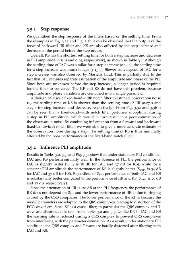
3.5 discussion 37
3.5.1 Step response
We quantified the step response of the filters based on the settling time. Fromthe examples in Fig. 3.3a and Fig. 3.3b it can be observed that the output of theforward-backward IIR filter and KS are also affected by the step increase anddecrease in the period before the step occurs.
Overall, KS has the shortest settling time for both a step increase and decreasein PLI amplitude (0.16 s and 0.14, respectively), as shown in Table 3.1. Althoughthe settling time of IAC was similar for a step decrease (0.14 s), the settling timefor a step increase was much longer (1.15 s). Slower convergence of IAC for astep increase was also observed by Martens [112]. This is partially due to thefact that IAC requires separate estimation of the amplitude and phase of the PLI.Since both are unknown before the step increase, a longer period is requiredfor the filter to converge. The KF and KS do not have this problem, becauseamplitude and phase variations are combined into a single parameter.
Although KS uses a fixed-bandwidth notch filter to estimate observation noisern, the settling time of KS is shorter than the settling time of IIR (0.27 s and0.29 s for step increase and decrease, respectively). From Fig. 3.3a and 3.3b itcan be seen that a fixed-bandwidth notch filter performs suboptimal duringa step in PLI amplitude, which would in turn result in a poor estimation ofthe observation noise. By combining information from a forward and backwardfixed-bandwidth notch filter, we were able to give a more accurate estimate ofthe observation noise during a step. The settling time of KS is thus minimallyaffected by the poor performance of the fixed-band notch filter.
3.5.2 Influence PLI amplitude
Results in Tables 3.2, 3.3, and Fig. 3.5a show that under stationary PLI conditions,IAC and KS perform similarly well. In the absence of PLI the performance ofIAC is slightly better (Sout is 38 dB for IAC and 37 dB for KS), while for aconstant PLI amplitude the performance of KS is slightly better (Sout is 34 dBfor IAC and 37 dB for KS). Regardless of Sin, performance of both IAC and KSis substantially better compared to the performance of IIR and KF (Sout is 20 dBand 17 dB, respectively).
Since the attenuation of IIR is -70 dB at the PLI frequency, the performance ofIIR does not depend on Sin and the lower performance of IIR is due to ringingcaused by the QRS complexes. The lower performance of the KF is because themodel parameters are adapted to the QRS complexes, leading to distortion of theECG waveform. Since KF is a causal filter, in particular the QRS complex and T-wave are distorted, as is seen from Tables 3.2 and 3.3. Unlike KF, in IAC and KSthe learning rate is reduced during a QRS complex to prevent QRS complexesfrom interfering with the parameter estimation. As a result, under stationary PLIconditions the QRS complex and T-wave are hardly distorted after filtering withIAC and KS.
[ March 26, 2018 at 22:26 – classicthesis version 4.2 ]
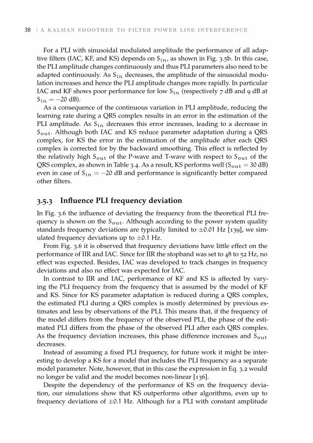
38 a kalman smoother to filter power line interference
For a PLI with sinusoidal modulated amplitude the performance of all adap-tive filters (IAC, KF, and KS) depends on Sin, as shown in Fig. 3.5b. In this case,the PLI amplitude changes continuously and thus PLI parameters also need to beadapted continuously. As Sin decreases, the amplitude of the sinusoidal modu-lation increases and hence the PLI amplitude changes more rapidly. In particularIAC and KF shows poor performance for low Sin (respectively 7 dB and 9 dB atSin = −20 dB).
As a consequence of the continuous variation in PLI amplitude, reducing thelearning rate during a QRS complex results in an error in the estimation of thePLI amplitude. As Sin decreases this error increases, leading to a decrease inSout. Although both IAC and KS reduce parameter adaptation during a QRScomplex, for KS the error in the estimation of the amplitude after each QRScomplex is corrected for by the backward smoothing. This effect is reflected bythe relatively high Sout of the P-wave and T-wave with respect to Sout of theQRS complex, as shown in Table 3.4. As a result, KS performs well (Sout = 30 dB)even in case of Sin = −20 dB and performance is significantly better comparedother filters.
3.5.3 Influence PLI frequency deviation
In Fig. 3.6 the influence of deviating the frequency from the theoretical PLI fre-quency is shown on the Sout. Although according to the power system qualitystandards frequency deviations are typically limited to ±0.01 Hz [139], we sim-ulated frequency deviations up to ±0.1 Hz.
From Fig. 3.6 it is observed that frequency deviations have little effect on theperformance of IIR and IAC. Since for IIR the stopband was set to 48 to 52 Hz, noeffect was expected. Besides, IAC was developed to track changes in frequencydeviations and also no effect was expected for IAC.
In contrast to IIR and IAC, performance of KF and KS is affected by vary-ing the PLI frequency from the frequency that is assumed by the model of KFand KS. Since for KS parameter adaptation is reduced during a QRS complex,the estimated PLI during a QRS complex is mostly determined by previous es-timates and less by observations of the PLI. This means that, if the frequency ofthe model differs from the frequency of the observed PLI, the phase of the esti-mated PLI differs from the phase of the observed PLI after each QRS complex.As the frequency deviation increases, this phase difference increases and Soutdecreases.
Instead of assuming a fixed PLI frequency, for future work it might be inter-esting to develop a KS for a model that includes the PLI frequency as a separatemodel parameter. Note, however, that in this case the expression in Eq. 3.2 wouldno longer be valid and the model becomes non-linear [136].
Despite the dependency of the performance of KS on the frequency devia-tion, our simulations show that KS outperforms other algorithms, even up tofrequency deviations of ±0.1 Hz. Although for a PLI with constant amplitude
[ March 26, 2018 at 22:26 – classicthesis version 4.2 ]

3.6 conclusion 39
and frequency deviation of ±0.1 Hz IAC has a better Sout (Sout is 35 dB forIAC and 29 dB for KS), the Sout for a PLI with sinusoidal modulated amplitudeis much worse (Sout is 7 dB for IAC and 29 dB for KS).
3.5.4 Computational complexity
The computational complexity of KS depends on the time delay used for the fil-ter (τfb and τ). Since for each new sample the smoothing needs to be performedover the entire delay, increasing the delay substantially contributes to the com-plexity. For the selected time delays in this study, the computation complexitywas in the order of 103 MPS. In contrast, IAC and KF are causal filters and theirMPS is much smaller (39 MPS and 50 MPS, respectively).
Despite the relatively high computational complexity with respect to the causalfilters, at a sampling rate of 500 Hz KS still only requires about 106 multiplica-tions per second. Assuming that the clock frequency of a modern DSP is in theorder of GHz (e.g. C6000™ series by Texas Instruments, Dallas, TX), KS only re-quires 0.1% of the entire capacity of the DSP. Therefore, real time implementationof KS should not be a problem.
For off-line applications it is possible to use a fixed-interval KS as an alter-native to a fixed-lag KS [140]. Instead of calculating smoothed estimates for afixed time lag τ, the fixed-interval KS gives smoothed estimates based on allobservations in the signal. The fixed-interval KS first runs the forward KF overthe entire signal, after which smoothed estimates are obtained by a backwardKS. Since this approach only requires a single forward and backward run, thecomputational complexity reduces to 129 MPS.
3.6 ConclusionIn this study, a linear fixed-lag KS was developed to suppress PLI in ECG record-ings. The developed KS outperforms other methods that have been proposed inthe literature in terms of step response settling time and output SNR. The pro-posed method can be used for semi real-time applications with a time delay of0.4 s.
[ March 26, 2018 at 22:26 – classicthesis version 4.2 ]

[ March 26, 2018 at 22:26 – classicthesis version 4.2 ]

4 H I E R A R C H I C A L B AY E S I A N F R A M E W O R K F O RF E TA L R - P E A K D E T E C T I O N , U S I N G E C GWAV E F O R M A N D H E A RT R AT E I N F O R M AT I O N
Abstract - The abdominal fetal electrocardiogram (ECG) can provide valuable infor-mation about fetal well-being. However, fetal R-peak detection in abdominal fetal ECGrecordings is challenging due to the low signal-to-noise ratio (SNR) and the non-stationary nature of the fetal ECG waveform in the abdominal recordings. In this paper,we propose a multichannel hierarchical Bayesian framework for fetal R-peak detection,that combines predictive models of the ECG waveform and the heart rate. The perfor-mance of our method was evaluated on set-A of the 2013 Physionet/Computing inCardiology Challenge and compared to the performance of several methods that havebeen proposed in the literature.The hierarchical Baysian framework presented in thisstudy outperforms other methods for fetal R-peak detection with a mean overall detectionaccuracy for set-A of 99.6%. Even for recordings with low SNR our method enablesreliable fetal R-peak detection (accuracy of 99.4%).1
1 This chapter has been submitted as Warmerdam G.J.J., Vullings R., Schmitt L., Van Laar J.O.E.H., andBergmans J.W.M., "Hierarchical Bayesian framework for fetal R-peak detection, using ECG waveform andheart rate information".
[ March 26, 2018 at 22:26 – classicthesis version 4.2 ]
42 hierarchical framework for r-peak detection
4.1 IntroductionSince the 1960s, the most widely used technique for fetal monitoring is car-diotocography (CTG) [5]. CTG provides simultaneous information on the fetalheart rate (FHR) and uterine activity. However, interpretation of CTG suffersfrom a low specificity, resulting in unnecessary operative deliveries [9].
To obtain additional information on fetal well-being in case of an abnormalCTG, the fetal electrocardiogram (ECG) could be used [19]. From the fetal ECGit is possible to extract beat-to-beat FHR information that is required for reliableanalysis of fetal heart rate variability (HRV) [42]. Moreover, analysis of the fetalECG waveform could provide information on fetal oxygen deficiency [1]. Bothfor HRV analysis and fetal ECG waveform analysis accurate R-peak detection isrequired.
Generally, the fetal ECG is obtained invasively using an electrode attached tothe fetal scalp [1]. Although the signal quality of invasive fetal ECG is good, itcan only be used during delivery after the fetal membranes have ruptured. Analternative that can also be used earlier in the pregnancy is to measure the fetalECG non-invasively by electrodes placed on the maternal abdomen [118].
The low invasiveness of the abdominal fetal ECG comes at a cost of a reductionin signal-to-noise ratio (SNR) [148]. The abdominal fetal ECG is contaminatedby electrical interferences such as the maternal ECG, muscle activity, power lineinterference, and measurement noise. Moreover, in the period between 28 to 32weeks of gestation, an isolating layer (the vernix caseosa) surrounds the fetusand reduces the amplitude and affects the shape of the abdominal fetal ECG[106].
In recent years, abdominal fetal ECG recordings have been extensively stud-ied, most studies focusing on suppression of the maternal ECG, which is thedominant interference [44, 118–123]. In 2013, the aim of the PhysioNet/Comput-ing in Cardiology Challenge (further referred to as Challenge) was to extract theFHR from abdominal recordings [149]. A variety of algorithms was presentedfor maternal ECG suppression, such as template subtraction [118–120], adaptivefiltering [44, 121], blind source separation (BSS) [122, 123, 125], or a combinationof different algorithms [126–128]. For an extensive review see [148] or [46]. Tocompare different algorithms, a database of abdominal fetal ECG recordings wasmade publicly available.
After maternal ECG suppression, fetal R-peak detection is often performedby adapting existing algorithms for adult R-peak detection [127, 128, 150]. How-ever, even after maternal ECG suppression, the SNR of the abdominal fetal ECGis generally still much lower than the SNR for adult ECG recordings. Since algo-rithms for adult R-peak detection are optimized for relatively high SNR, this canlead to numerous mis-detections for the low-SNR abdominal fetal ECG.
Besides low SNR, the position and orientation of the fetus within the abdomenare a priori unknown and can change during a recording. Therefore, the ab-dominal fetal ECG is typically recorded using multiple electrodes spread across
[ March 26, 2018 at 22:26 – classicthesis version 4.2 ]
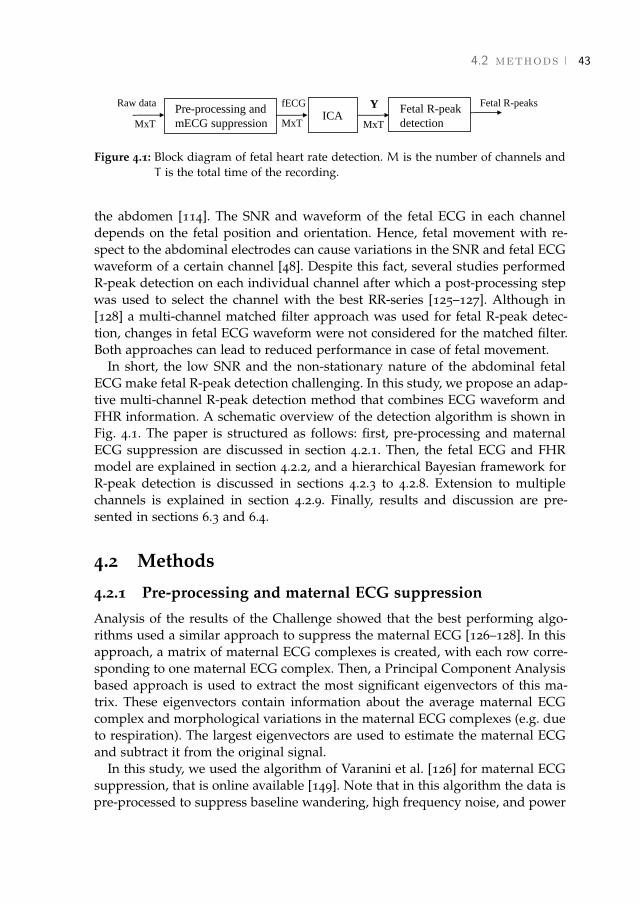
4.2 methods 43
Pre-processing and
mECG suppressionICA
Fetal R-peak
detection
Raw data fECG Fetal R-peaksY
MxT MxT MxT
Figure 4.1: Block diagram of fetal heart rate detection. M is the number of channels andT is the total time of the recording.
the abdomen [114]. The SNR and waveform of the fetal ECG in each channeldepends on the fetal position and orientation. Hence, fetal movement with re-spect to the abdominal electrodes can cause variations in the SNR and fetal ECGwaveform of a certain channel [48]. Despite this fact, several studies performedR-peak detection on each individual channel after which a post-processing stepwas used to select the channel with the best RR-series [125–127]. Although in[128] a multi-channel matched filter approach was used for fetal R-peak detec-tion, changes in fetal ECG waveform were not considered for the matched filter.Both approaches can lead to reduced performance in case of fetal movement.
In short, the low SNR and the non-stationary nature of the abdominal fetalECG make fetal R-peak detection challenging. In this study, we propose an adap-tive multi-channel R-peak detection method that combines ECG waveform andFHR information. A schematic overview of the detection algorithm is shown inFig. 4.1. The paper is structured as follows: first, pre-processing and maternalECG suppression are discussed in section 4.2.1. Then, the fetal ECG and FHRmodel are explained in section 4.2.2, and a hierarchical Bayesian framework forR-peak detection is discussed in sections 4.2.3 to 4.2.8. Extension to multiplechannels is explained in section 4.2.9. Finally, results and discussion are pre-sented in sections 6.3 and 6.4.
4.2 Methods
4.2.1 Pre-processing and maternal ECG suppression
Analysis of the results of the Challenge showed that the best performing algo-rithms used a similar approach to suppress the maternal ECG [126–128]. In thisapproach, a matrix of maternal ECG complexes is created, with each row corre-sponding to one maternal ECG complex. Then, a Principal Component Analysisbased approach is used to extract the most significant eigenvectors of this ma-trix. These eigenvectors contain information about the average maternal ECGcomplex and morphological variations in the maternal ECG complexes (e.g. dueto respiration). The largest eigenvectors are used to estimate the maternal ECGand subtract it from the original signal.
In this study, we used the algorithm of Varanini et al. [126] for maternal ECGsuppression, that is online available [149]. Note that in this algorithm the data ispre-processed to suppress baseline wandering, high frequency noise, and power
[ March 26, 2018 at 22:26 – classicthesis version 4.2 ]

44 hierarchical framework for r-peak detection
0 1 2 3 4
time (sec)
ch4
ch3
ch2
ch1
(a) Raw signals (maternal andfetal ECG).
0 1 2 3 4
time (sec)
ch4
ch3
ch2
ch1
(b) Fetal ECG.
0 1 2 3 4
time (sec)
IC4
IC3
IC2
IC1
(c) Fetal ECG after ICA (Y).
Figure 4.2: Signals before and after pre-processing, maternal ECG suppression, and ICA.
line interference. After pre-processing and maternal ECG suppression, Indepen-dent Component Analysis (ICA) is used to further enhance the fetal ECG. Sinceour study focuses on fetal R-peak detection, the method of Varanini is not dis-cussed in detail and we will use the signals after maternal ECG suppressionand ICA (Y) as starting point for our fetal R-peak detection method. An exam-ple of the original signals, the fetal ECG after pre-processing and maternal ECGsuppression, and Y are shown in Fig. 4.2.
4.2.2 Fetal ECG model
We now proceed with a single channel approach (sections 4.2.2-4.2.8) and thenextend our model to multiple channels in section 4.2.9. A single ECG signal afterpre-processing, maternal ECG suppression, and ICA is denoted as y(t), where tis a time index. The location of the k-th fetal R-peak is denoted as µk, and thek-th RR-interval as wk = µk − µk−1.
Gaussian QRS model
In abdominal fetal ECG recordings, the amplitude of the fetal QRS complex isgenerally large compared to other segments of the fetal ECG (the P-, and T-wave). Therefore, our model for R-peak detection is limited to describing thefetal QRS complex. It is important that the QRS model is flexible, because it isa priori unknown what the fetal orientation and location is with respect to theabdominal electrodes.
Our QRS model is inspired by a model that was proposed by McSharry et al.,which uses Gaussian kernels to describe the fetal ECG [151, 152]. A disadvantageof the model of McSharry is that a relatively large number of parameters is
[ March 26, 2018 at 22:26 – classicthesis version 4.2 ]

4.2 methods 45
-20 0 20time (ms)
a.u.
-20 0 20time (ms)
a.u.
-20 0 20time (ms)
a.u.
Figure 4.3: Example QRS model. From left to right: Gaussian, first derivative, and secondderivative.
required to described the QRS complex (nine parameters in total). Moreover, thelocations of the Q- and S-peak need to be determined with respect to the R-peak.
As noted by Biglari et al., the abdominal fetal ECG is recorded at far-field andthe morphology of the QRS complex is not as diverse and complex as for theadult ECG [50]. In our approach, the QRS complex is modeled by the sum ofa Gaussian (mainly modeling the R-wave), its first derivative (mainly modelingthe Q- and S-wave), and its second derivative (modeling the Q-, R-, and S-wave).Examples of these functions are shown in Fig. 4.3. The combination of thesefunctions can be used to describe the QRS complex for most abdominal fetalECG recordings [50].
Assuming that the Gaussian, its first, and second derivative are centeredaround time µk, our QRS model is written as
G(t,µk, z) =(a1 + a2(t− µk) + a3(1−
(t− µk)2
b2))e
−(t−µk)2
2b2 , (4.1)
where z = [a1,a2,a3,b], and a1,2,3 are the amplitudes of the Gaussian, its firstand its second derivative. Note that for the first and second derivative a factor1/b2 is included in terms a2 and a3, respectively. The QRS model in Eq. 4.1depends on four parameters and does not require knowledge on the location ofthe Q- and S-peak.
Besides containing the fetal QRS complex, y(t) will be contaminated by electri-cal interferences, such as muscle artifacts, remainders of the maternal ECG, andmeasurement noise. These inferences are represented by an additive noise termξt, which will be referred to as the observation noise of the QRS model. Becauseξt is a combination of several signals, including measurement noise, we will as-sume ξt to have a zero-mean Gaussian distribution with variance λt. Given thelocation of the k+ 1-th R-peak, µk+1, we can write y(t) during the k+ 1-th QRScomplex as:
y(t) = G(t,µk+1, z) + ξt ξt ∼ N(0, λt). (4.2)
[ March 26, 2018 at 22:26 – classicthesis version 4.2 ]

46 hierarchical framework for r-peak detection
Since for each (regular) heartbeat the electrical activity of the fetal heart prop-agates in a similar way through the heart, the electrical activity will be similaracross heartbeats. However, the electrical activity measured by the abdominalelectrodes can vary over time due to fetal movement with respect to the elec-trodes. Assuming that during a ventricular contraction the fetal orientation re-mains constant, we can express the model parameters of the k+ 1-th QRS com-plex as
zk+1 = zk +ηk ηk ∼ N(0,Σk). (4.3)
Here, variations in zk are assumed to be described by a zero-mean Gaussianrandom walk process ηk, with [4× 4] covariance matrix Σk. We refer to ηk asthe process noise of the QRS model.
Time-varying autoregressive FHR model
To describe the fetal HR, we use a p-th order time-varying autoregressive(TVAR) model [153, 154]. In the TVAR model the k + 1-th RR-interval wk+1is described as a linear combination of p previously detected RR-intervalswk = [wk,wk−1, ...,wk−p+1]T . Since wk+1 = µk+1 −µk, we can use this modelto predict the location of µk+1, given previous RR-intervals and µk. The orderof the TVAR model was empirically determined and set to p = 6. The TVARmodel is written as
wk+1 = wTkθ+ vk+1 vk+1 ∼ N(0,Rk+1), (4.4)
with θ = [θ1, ...,θp]T the TVAR model parameters. In Eq. 4.4, any variation in theFHR that cannot be captured by the linear TVAR model is represented by vk+1.We refer to vk+1 as the observation noise of the FHR model and it is assumed tobe zero-mean Gaussian with variance Rk+1.
Because variations in the FHR are regulated by the autonomic nervous sys-tem and the autonomic regulation varies over time (e.g. due to changes in fetalbehavioral states [87]), parameters θ are also time-varying. We will assume thatvariations in θ can be modeled by a zero mean Gaussian dk, with [p× p] covari-ance Qk:
θk+1 = θk +dk dk ∼ N(0,Qk). (4.5)
The noise term dk is referred to as the process noise of the FHR model.
4.2.3 Hierarchical Bayesian framework
Given µk and the estimated k+ 1-th RR-interval wk+1, we will look for the nextR-peak µk+1 within a predefined search window. The search window is limitedto the interval t = µk+ wk+1± T2 , with T the width of the search window (set to400 ms). The search window is further limited by a minimum and maximum RR-interval (RRmin and RRmax, respectively), that are defined based on a range of
[ March 26, 2018 at 22:26 – classicthesis version 4.2 ]

4.2 methods 47
𝜇𝑘+1 𝒛𝑘+1, 𝜽𝑘+1 𝚺𝑘+1, 𝚲𝑘+1,𝑸𝑘+1, 𝑅𝑘+1Φ𝑘
𝒚𝑘+1Level 1:
State estimation
R-peak prediction
Level 3:
Noise estimation
Φ𝑘+1
Increment k
Level 2:
Model estimation
Figure 4.4: Schematic overview of the hierarchical model.
the FHR between 50 and 210 beats per minute (bpm) [1]. The observation noisein yk+1 is described by ξk+1, with covariance Λk+1. Notice that with respect toEq. 4.2, we have changed from scalar to vector notation.
Based on this description of yk+1 and 4.4 we can define a state-space modelfor the k+ 1-th QRS complex:
µk+1 = µk +wTkθk+1 + vk+1 vk+1 ∼ N(0,Rk+1)
yk+1 = G(t,µk+1, zk+1) + ξk+1 ξk+1 ∼ N(0,Λk+1),(4.6)
Given yk+1, we are interested in estimating the new R-peak location µk+1. Theuncertainties in the state-space model in Eq. 4.6 suggest that a probabilistic ap-proach can be used to solve the estimation problem for µk+1. To find a tractablesolution for inferring µk+1, we propose a hierarchical probabilistic frameworkthat consists of three inference levels:Level 1: State estimation. In this level, we estimate µ, while assuming that θ, z,and covariances Q, R, Σ, and Λ are known.Level 2: QRS and FHR model estimation. In this level, we estimate θ and z,while assuming µ, Q, R, Σ, and Λ to be known.Level 3: Noise estimation. In this level, we estimate Q, R, Σ, and Λ, while as-suming µ, θ, and z to be known.
A schematic overview of the inference is presented in Fig. 4.4. Note that weused different inference strategies to estimate the model parameters (as summa-rized in Table 4.1), hence our hierarchical model is not fully Bayesian.
4.2.4 Level 1: State estimation
Given the estimated model parameters after observing the k-th QRS complexand new observation yk+1, we want to predict the location of the k+ 1-th QRScomplex. Using Bayes’ rule we can describe the posterior probability density func-tion for µk+1 as
p(µk+1|yk+1,Φk) =p(yk+1|µk+1,Φk)p(µk+1|yk,Φk)
p(yk+1|yk,Φk), (4.7)
[ March 26, 2018 at 22:26 – classicthesis version 4.2 ]

48 hierarchical framework for r-peak detection
Table 4.1: Model parameters (Φ) and inference strategy.
Parameter Estimation strategy
µ MAPz EKFθ KFΣ empirically determinedΛ from signalQ maximum likelihoodR empirically determined
with Φk = {µk, zk,θk,wk,Σk,Λk,Qk,Rk} our prior information about themodel parameters from the previous iteration.
Because p(yk+1|yk,Φk) is a normalization factor that is independent of µk+1,the maximum a posteriori (MAP) estimate for µk+1 can be written as:
µk+1 = argmaxµk+1
(lnp(yk+1|µk+1,Φk) + lnp(µk+1|yk,Φk)
), (4.8)
where the use of the log-posterior is justified by the monotonic behavior of thelogarithm, which will not influence the MAP solution. In the next levels µk+1 isused to estimate the model parameters and noise covariances.
4.2.5 Level 2: QRS and FHR model estimation
Given observation yk+1 and the location of the k+ 1-th R-peak at µk+1, we wantto update our model parameters θ and z. We will assume that the FHR does notinfluence the QRS waveform, and consider θ and z to be independent.
Extended Kalman filter to estimate QRS model
Using the QRS model that is explained in section 4.2.2, we can describe thewaveform of the k+ 1-th QRS complex by the following state-space equations:
zk+1 = zk +ηk ηk ∼ N(0,Σk)
yk+1 = G(t, µk+1, zk+1) + ξk+1 ξk+1 ∼ N(0,Λk+1).(4.9)
A tractable approximation for the MAP estimate zk+1 for zk+1 of this non-linearstate-space model can be calculated using an Extended Kalman Filter (EKF) [140].In the EKF formalism, a first order approximation is used to describe the non-linear function G(t, µk+1, zk). Note that the EKF provides the minimum mean
[ March 26, 2018 at 22:26 – classicthesis version 4.2 ]

4.2 methods 49
square error estimate, which is not necessarily identical to the MAP estimate incase of a non-linear model. The EKF update equations are given by [140]:
zk+1 = zk +KQRSk+1 (yk+1 −G(t, µk+1, zk)) (4.10)
Pk+1 = Pk +Σk −KQRSk+1 J
Tk+1(Pk +Σk) (4.11)
KQRSk+1 = (Pk +Σk)Jk+1(J
Tk+1(Pk +Σk)Jk+1 +Λk+1)
−1, (4.12)
with Pk the [4× 4] covariance in zk, KQRSk+1 the [4× T ] Kalman gain of the QRS
model, and Jk+1 the [4× T ] Jacobian matrix Jk+1 = ∂G∂z
∣∣∣(z=zk)
.
Kalman filter to estimate FHR model
Using the FHR model that is explained in section 4.2.2, the k+ 1-th RR-intervalcan be described by the following state-space equations:
θk+1 = θk +dk dk ∼ N(0,Qk)
wk+1 = wTkθk+1 + vk+1 vk+1 ∼ N(0,Rk+1).(4.13)
Following a similar derivation as in [143], it is possible to show that the MAPestimate θk+1 for θk+1 can be calculated using the linear Kalman filter updateequations:
θk+1 = θk +KHRk+1(wk+1 −w
Tkθk) (4.14)
Vk+1 = Vk +Qk −KHRk+1w
Tk(Vk +Qk) (4.15)
KHRk+1 =(Vk +Qk)wk
wTk(Vk +Qk)wk + Rk+1, (4.16)
where Vk is the [p× p] covariance of θk and KHRk+1 is the [p× 1] Kalman gain forthe FHR model.
4.2.6 Level 3: Noise estimation
Process noise Σk+1 of QRS model
Variations in the QRS waveform due to e.g. fetal movement are described bythe process noise Σk+1. We assume identical and uncorrelated process noisefor all QRS model parameters a = [a1, ...,a3]T . The process noise varianceσ2a is assumed constant, and is defined as a fraction of the maximum of thesquared average QRS complex in the initialization phase (see section 4.2.8): σ2a =
camax |QRS|2, where fraction ca is empirically determined. Furthermore, al-though the width of the fetal QRS complex can vary during pregnancy, fetalmovement will have little effect on the width. Hence the width is assumed to re-main constant throughout a recording. Therefore, we assume zero process noise
[ March 26, 2018 at 22:26 – classicthesis version 4.2 ]
50 hierarchical framework for r-peak detection
for parameter b, which means that b is estimated recursively. The process noiseΣk+1 for zk+1 is thus described as
Σk+1 = Σ =
σ2a 0
σ2aσ2a
0 0
. (4.17)
Observation noise Λk+1 of QRS model
To estimate the covariance Λk+1, we will assume that the observation noiseis uncorrelated and constant for observation yk+1. Note that since ξk+1 alsodescribes correlated physiological noise (i.e. muscle activity) this assumption isonly approximately true. The covariance matrix can then be written as Λk+1 =
λk+1IT . with IT the [T × T ] identity matrix.The estimation of λk+1 is based on the variance in yk+1. Typically, the dura-
tion of the fetal QRS complex is about L = 40 ms [138], which is about 10% ofa fetal ECG complex (assuming a heart rate of 150 bpm). In the state estimationin level 1 (where the location of µk+1 is estimated), the contribution of the QRScomplex to the variance of yk+1 is accounted for by omitting the top 10% of thevalues of yk+1. For the estimation of zk+1 in level 2 we update our estimateof λk+1 by omitting samples of yk+1 within the region µk+1 ± L2 . The value ofλk+1 is determined as the variance in yk+1 over the remaining samples.
Process noise Qk+1 of FHR model
In a hierarchical Bayesian model, the likelihood function at a particular level isequal to the evidence at the next higher level [143]. This means that by maxi-mizing the evidence of the FHR model in level 2 we can obtain the maximumlikelihood solution for Q.
The evidence of the FHR model is given by:
p(wk+1|yk+1,Φk) = N(wk+1|wTkθk,wTk(Qk +Vk)wk + Rk+1). (4.18)
The value of Qk+1 can be calculated by differentiating Eq. 4.18 with respect toQ and equating it to zero. If we assume that Qk+1 = qk+1Ip and define theresidual error of the FHR model as rk+1 = wk+1 −w
Tkθk, it can be shown that
the maximum likelihood estimate for qk+1 is [143]:
qk+1 =
r2k+1−E[r2k+1|qk+1=0]
wTkwk
if qk+1 > 0
0 otherwise(4.19)
Here E[r2k+1|qk+1 = 0] = wTkVkwk + Rk+1, is the covariance of rk+1 if weassume that qk+1 = 0. Eq. 4.19 implies that, if rk+1 is larger than the predictedvariance, the value of qk+1 increases. If qk+1 increases, the Kalman gain KHR
also increases and a new estimate of θ will depend more on incoming data.
[ March 26, 2018 at 22:26 – classicthesis version 4.2 ]

4.2 methods 51
Observation noise Rk+1 of FHR model
Following discussions on HRV, we know that variations in the heart rate oftencannot be fully described by a linear model [95]. This means that even in casewe have optimally inferred θ, we can only approximate a new RR-interval up toa certain degree. Any stochastic or non-linear variation in the FHR is describedby Rk+1.
Since the value of Rk+1 defines how well we expect our linear model to de-scribe the FHR, we will assume that Rk+1 = R0 is constant. A low value of R0leads to relatively high values of Q through Eq. 4.19. This means that θ will beadapted even for a small residual error. A large value of R0 leads to relativelylow values of Q. In this case adaptation of θ is reduced, which allows for largerdiscrepancies between the predicted FHR and the observed FHR. The value forR0 was empirically determined.
4.2.7 R-peak prediction
We can use our estimates for zk and θk at the k-th iteration to predict the R-peaklocation at the k+1-th iteration. Accounting for the covariances in our estimationof zk and θk (denoted by Pk and Vk, respectively), and making use of the statespace model in Eq. 4.6, we can write:
p(µk+1|yk,Φk) = N(µk+1|µk + wk+1, ΓHR), and (4.20)
p(yk+1|µk+1,Φk) = N(yk+1|yk+1, ΓQRS), (4.21)
with
wk+1 = wTkθk, (4.22)
ΓHR = wTk(Vk +Qk)wk + Rk+1, (4.23)
yk+1 = G(t,µk+1, zk), and (4.24)
ΓQRS = JTk+1(Pk +Σk)Jk+1 +Λk+1. (4.25)
Hence, the log-posterior for µk+1 in Eq. 4.8 can be written as:
L = const. −(µk+1 − µk − wk+1)
2
ΓHR
− (yk+1 − yk+1)TΓQRS
−1(yk+1 − yk+1). (4.26)
Notice that yk+1 depends on µk+1 through the function G(t,µk+1, zk). Further-more, L can be multimodal and is necessarily not Gaussian.
Regardless of the signal quality, it is always possible to find a µk+1 that max-imizes L. However, in case of poor signal quality µk+1 might be inaccurate,leading to mis-detections of the R-peak. To prevent mis-detection, a sanity checkis performed during which we compare the probability that µk+1 is the locationof an R-peak to the probability that µk+1 is not the location of an R-peak.
[ March 26, 2018 at 22:26 – classicthesis version 4.2 ]
52 hierarchical framework for r-peak detection
Focusing on the samples during a QRS complex i = µk+1± L2 , we can comparethe likelihood for yi = y(i) in case µk+1 is an R-peak to the likelihood for yiin case µk+1 is not an R-peak. If µk+1 is an R-peak, the likelihood for yi isp(yi|µk+1 = R-peak) = N(yi|yi, ΓQRS). If µk+1 is not the location of an R-peak,the likelihood for yi is p(yi|µk+1 6= R-peak) = N(yi|0,Λk+1). This means that:
µk+1
{= R-peak, if (yi − yi)TΓ
QRS−1
k+1 (yi − yi) < yTi Λ
−1k+1yi
6= R-peak, otherwise(4.27)
If according to Eq. 4.27 µk+1 is the location of an R-peak, we use µk+1 inlevels 2 and 3 to estimate the model parameters and noise covariances. In caseµk+1 is not the location of an R-peak according to Eq. 4.27, the model parame-ters and noise covariances are not updated. Instead, we extrapolate an R-peaklocation based on the FHR model and continue to predict µk+2 given the priorinformation Φk (i.e. predict p(µk+2|yk+2,Φk)). In case more than five consecu-tive detected peaks were no R-peaks according to Eq. 4.27, the entire algorithmis re-initialized (see section 4.2.8).
4.2.8 Parameter initialization
In the (re-)initialization phase, a segment of 10 seconds is used to obtain es-timates for Φ0 = {µ0, z0,θ0,w0,Λ0,Σ,Q0,R}. During initialization, the QRSmodel described by Eq. 4.1 is used as a frequency bandpass filter with a peakfrequency of 42 Hz[150]. After filtering, a simple local maximum search is usedfor peak detection, where each search window is defined based on a previousmaximum.
The detected peaks within the segment are used to calculate an average QRScomplex, from which initial estimates z0 are obtained using a least-squares ap-proach. Furthermore, RR-intervals are calculated from the detected peaks andRR-intervals outside a range of RRmin to RRmax are removed. On the remain-ing RR-intervals a Yule-Walker method is used to obtain initial estimates θ0. Thefirst R-peak is used as µ0 and the first p RR-intervals were used as w0.
Initial covariances of the QRS model Σ and Λ0 are calculated as described inSection 4.2.6 and 4.2.6, and we initialized P0 = 3Σ. Initial covariances of the FHRmodel were set to Q0 = 10−4max |θ0|2, R = R0, and V0 = Q0.
If forward prediction fails (i.e. more than five consecutive detected peakswere no R-peaks according to Eq. 4.27) and new parameters were found in re-initialization, we can use future information to obtain smoothed estimates ofany missed (or mis-detected) R-peaks in the period before the start of the re-initialization. In essence, backwards prediction is similar to forward prediction,with the difference that the FHR and QRS model are trained in the backwards
[ March 26, 2018 at 22:26 – classicthesis version 4.2 ]

4.2 methods 53
direction. By combining the information of our forwards prediction and back-wards prediction we obtain smoothed estimates for µk+1:
p(µk+1|yk+1,yk+2,Φk,Φk+2) ∝ p(µk+1|yk+1,Φk)
· p(µk+1|yk+2,Φk+2). (4.28)
4.2.9 Multichannel extension
As described before, the abdominal ECG is commonly recorded from multiplechannels. Because the ECG signals are correlated, recording the ECG on multiplechannels can be exploited to improve the signal to noise conditions.
The model in Eq. 4.9 can be extended toM electrodes by training a QRS modelto each channel. Assuming that the noise in each channel is uncorrelated, we canwrite
y(1)k+1 = G(t, µk+1, z(1)k+1) + ξ
(1)k+1 ξ
(1)k+1 ∼ N(0,Λ(1)
k+1)
...
y(M)k+1 = G(t, µk+1, z(M)
k+1) + ξ(M)k+1 ξ
(M)k+1 ∼ N(0,Λ(M)
k+1), (4.29)
with z(m)k+1 = [a
(m)k+1,b(m)]. Since the width of the QRS complex is similar for all
channels, we only need to estimate one width parameter b = b(1), ...,b(M).We can write a similar state-space model as the single channel ECG in Eq. 4.9
for the multichannel ECG:
zak+1 = zak +ηak ηak ∼ N(0,Σak)
yak+1 = G(t, µk+1, zak+1) + ξak+1 ξak+1 ∼ N(0,Λak+1).
(4.30)
Here, we defined the multichannel state and observation vectors as:
zak = [a(1)k , ...,a(M)
k ,b]T and (4.31)
yak+1 = [y(1)k+1, ...,y(M)
k+1]T , (4.32)
and the multichannel noise covariances as:
Σak =
σ2aI3 0
. . .σ2aI3
0 0
and (4.33)
Λak =
Λ
(1)k 0
. . .
0 Λ(M)k
. (4.34)
A similar approach can be used as the one discussed in section 4.2.5 to calculatethe MAP estimate zak+1 for zak+1.
[ March 26, 2018 at 22:26 – classicthesis version 4.2 ]

54 hierarchical framework for r-peak detection
4.2.10 Algorithms from the literature
The performance of our algorithm is compared to the performance of the algo-rithms of Varanini et al. [126] and Behar et al. [127], both scored high in theChallenge and have source codes that were online available. Besides algorithmsfrom the Challenge, we also implemented the algorithm of Biglari et al. [50], be-cause they used similar (fixed) templates for peak detection as our QRS modelpresented in Eq. 4.1.
Our pre-processing for maternal ECG suppression is equal to the one usedby Varanini. After maternal ECG suppression and ICA, Varanini performs fetalR-peak detection on all individual channels and the channel with the best fetalRR-series is selected. Varanini uses a two step fetal R-peak detection. In the firststep, potential fetal R-peaks are detected using a derivative filter. In the secondstep a forward and backward TVAR model is trained on the RR-series from thefirst step, starting from an RR-interval that is closest to the mode RR-interval.The forward and backward TVAR model are then used in combination with thederivative signal to detect the fetal R-peaks. After R-peak detection, the channelwith the best RR-series is selected based on some statistical features of the RR-series.
For the algorithm of Biglari we used the same maternal ECG suppression asthe one proposed by Varanini. After maternal ECG suppression, Biglari usespredefined templates for fetal R-peak detection that are based on most commonfetal QRS morphologies. Fetal R-peaks are detected in each channel separately.First, each channel is passed through the matched filters using normalized cross-correlation. From the cross-correlated signals, the vectorcardiogram amplitude(VA) [44] is calculated per channel, which is then used to detect the fetal R-peakswith a local search algorithm over a sliding window [44]. Finally, channels wereranked according to the robust weighted average [155] and the R-peaks from thechannel with the highest rank were stored.
The algorithm of Behar uses a combination of template subtraction techniquesand BSS techniques to suppress the maternal ECG and enhance the fetal ECGafter maternal ECG suppression [127]. Then, fetal R-peak detection is performedon all generated signals using an adapted version of the Pan and Tomkins al-gorithm [156] and a quality index is used to select the best RR-series. Finally,a smoothing step is performed to remove extra detected fetal R-peaks and fixmissed fetal R-peaks. Note that we unchecked the cinc-match option, since thisreduced the performance of the algorithm of Behar.
4.3 Data acquisition and evaluationWe used simulations to evaluate the flexibility of our algorithm for changingconditions of the fetal ECG morphology due to fetal movement. We assumedthat the maternal ECG was already suppressed and used the model presentedin [44] to simulate the fetal ECG. This model assumes that the electrical activity
[ March 26, 2018 at 22:26 – classicthesis version 4.2 ]

4.3 data acquisition and evaluation 55
of the heart (at far-field) can be approximated by a single dipole field vector.The three-dimensional path that is described by this vector over time is calledthe vectorcardiogram (VCG). The ECG is a projection of the field vector ontoelectrode leads. We simulated a full rotation of the fetus within the abdomen bychanging the position and orientation of the VCG with respect to a vertical andhorizontal electrode lead (as shown in Fig. 4.5a). Similar to [44], non-stationarynoise was generated based on real noise signals (muscle artifacts and electrodemovements) that can be obtained in the MIT-BIH non-stress test database [157].Note that we did not consider baseline wander, because this would be removedby high-pass frequency filtering in maternal ECG suppression [126].
To evaluate our method we used the set-A of the 2013 Physionet/Comput-ing in Cardiology Challenge [149]. The database consists of 75 abdominal ECGrecordings, measured with four channels at a sampling rate of 1000 Hz. For set-A, the reference fetal R-peaks are provided. Recordings a33, a38, a52, a54, a71,and a74 were excluded due to partially missing annotations [126, 127], leaving69 recordings for evaluation.
The performance of the R-peak detection is evaluated by comparing the de-tected fetal R-peaks to the annotated peaks. As evaluation metrics we used theaccuracy (Ac):
Ac =TP
TP + FN + FP. (4.35)
Here, TP is the number of correctly detected fetal R-peaks, FN is the number ofmissed R-peaks, and FP is the number of falsely detected R-peaks. A detectedR-peak is considered a TP if it falls within a window of 50 ms from an annotatedpeak [125, 127].
To determine the performance for different SNR conditions, we calculated anaverage SNR for each recording and split the data-set into three groups: record-ings with low SNR (lowest 10%), median SNR (middle group), and high SNR(highest 10%). We calculated the SNR in the signals after maternal ECG sup-pression and ICA, because these are the signals that were used for fetal R-peakdetection. For each annotated R-peak in each IC, the SNR was calculated as:
S = 10 log10( PsPn
), (4.36)
with Ps the power of the QRS complex and Pn the power of the noise. Ps wascalculated as the variance in a window of ±20 ms surrounding the annotatedR-peak and Pn as the variance in a window of [-150:-20 20:150] ms surroundingthe annotated R-peak. The average SNR was calculated for each IC and the SNRof a recording was defined as the maximum average SNR.
Note that we did not consider evaluation metrics for heart rate estimation(e.g. mean-squared-error (MSE) between detected and annotated heat rate). Post-processing techniques such as those proposed in [125] or [127] could be used toimprove the FHR estimation, but this is outside the scope of this study. For the
[ March 26, 2018 at 22:26 – classicthesis version 4.2 ]
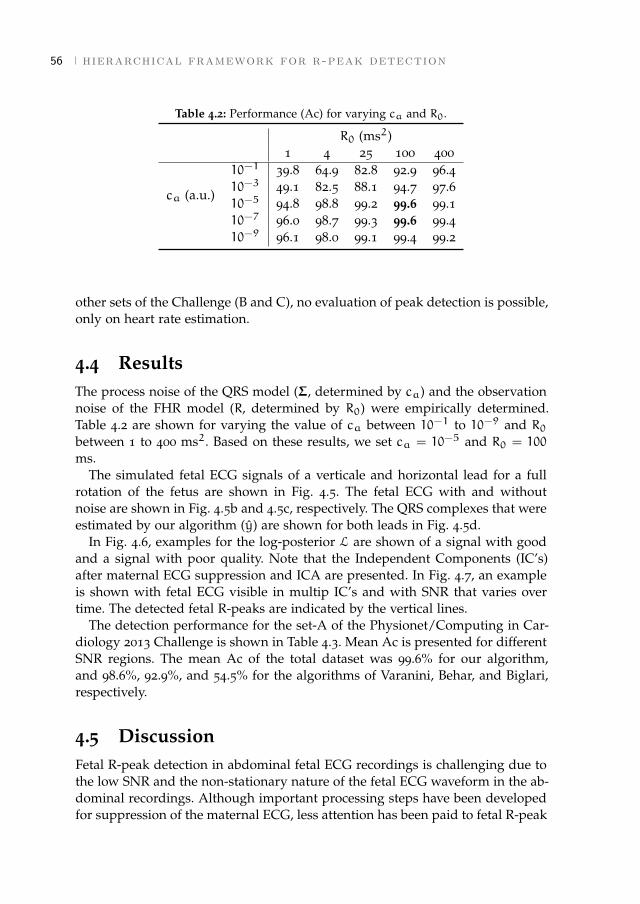
56 hierarchical framework for r-peak detection
Table 4.2: Performance (Ac) for varying ca and R0.
R0 (ms2)1 4 25 100 400
10−1 39.8 64.9 82.8 92.9 96.4
ca (a.u.)10−3 49.1 82.5 88.1 94.7 97.610−5 94.8 98.8 99.2 99.6 99.110−7 96.0 98.7 99.3 99.6 99.410−9 96.1 98.0 99.1 99.4 99.2
other sets of the Challenge (B and C), no evaluation of peak detection is possible,only on heart rate estimation.
4.4 ResultsThe process noise of the QRS model (Σ, determined by ca) and the observationnoise of the FHR model (R, determined by R0) were empirically determined.Table 4.2 are shown for varying the value of ca between 10−1 to 10−9 and R0between 1 to 400 ms2. Based on these results, we set ca = 10−5 and R0 = 100
ms.The simulated fetal ECG signals of a verticale and horizontal lead for a full
rotation of the fetus are shown in Fig. 4.5. The fetal ECG with and withoutnoise are shown in Fig. 4.5b and 4.5c, respectively. The QRS complexes that wereestimated by our algorithm (y) are shown for both leads in Fig. 4.5d.
In Fig. 4.6, examples for the log-posterior L are shown of a signal with goodand a signal with poor quality. Note that the Independent Components (IC’s)after maternal ECG suppression and ICA are presented. In Fig. 4.7, an exampleis shown with fetal ECG visible in multip IC’s and with SNR that varies overtime. The detected fetal R-peaks are indicated by the vertical lines.
The detection performance for the set-A of the Physionet/Computing in Car-diology 2013 Challenge is shown in Table 4.3. Mean Ac is presented for differentSNR regions. The mean Ac of the total dataset was 99.6% for our algorithm,and 98.6%, 92.9%, and 54.5% for the algorithms of Varanini, Behar, and Biglari,respectively.
4.5 DiscussionFetal R-peak detection in abdominal fetal ECG recordings is challenging due tothe low SNR and the non-stationary nature of the fetal ECG waveform in the ab-dominal recordings. Although important processing steps have been developedfor suppression of the maternal ECG, less attention has been paid to fetal R-peak
[ March 26, 2018 at 22:26 – classicthesis version 4.2 ]
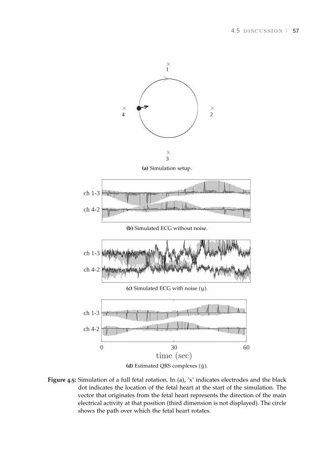
4.5 discussion 57
2
3
4
1
(a) Simulation setup.
ch 4-2
ch 1-3
(b) Simulated ECG without noise.
ch 4-2
ch 1-3
(c) Simulated ECG with noise (y).
0 30 60time (sec)
ch 4-2
ch 1-3
(d) Estimated QRS complexes (y).
Figure 4.5: Simulation of a full fetal rotation. In (a), ’x’ indicates electrodes and the blackdot indicates the location of the fetal heart at the start of the simulation. Thevector that originates from the fetal heart represents the direction of the mainelectrical activity at that position (third dimension is not displayed). The circleshows the path over which the fetal heart rotates.
[ March 26, 2018 at 22:26 – classicthesis version 4.2 ]

58 hierarchical framework for r-peak detection
0 0.25 0.5time (sec)
IC4
IC3
IC2
IC1
yk+1 yk+1
0 0.25 0.5
a.u.
ln p(µk+1|yk,Φk)ln p(yk+1|µk+1,Φk)
0 0.25 0.5time (sec)
a.u.
ln p(µk+1|yk+1,Φ)
(a) Good signal quality.
0 0.25 0.5time (sec)
IC4
IC3
IC2
IC1
yk+1 yk+1
0 0.25 0.5
a.u.
ln p(µk+1|yk,Φk)ln p(yk+1|µk+1,Φk)
0 0.25 0.5time (sec)
a.u.
ln p(µk+1|yk+1,Φ)
(b) Poor signal quality.
Figure 4.6: Example of good (a) and poor (b) quality signal. The verticale line show thelocation of the annotated R-peak. In case of good quality, the QRS model dom-inates the posterior, while in case of poor quality the FHR model dominatesthe posterior.
[ March 26, 2018 at 22:26 – classicthesis version 4.2 ]
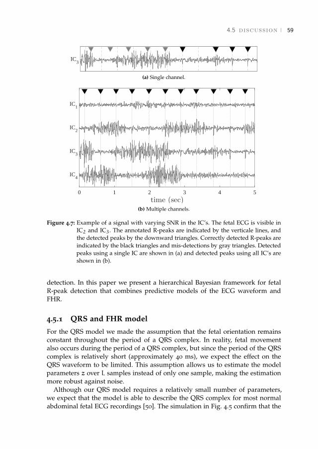
4.5 discussion 59
IC3
(a) Single channel.
0 1 2 3 4 5time (sec)
IC4
IC3
IC2
IC1
(b) Multiple channels.
Figure 4.7: Example of a signal with varying SNR in the IC’s. The fetal ECG is visible inIC2 and IC3. The annotated R-peaks are indicated by the verticale lines, andthe detected peaks by the downward triangles. Correctly detected R-peaks areindicated by the black triangles and mis-detections by gray triangles. Detectedpeaks using a single IC are shown in (a) and detected peaks using all IC’s areshown in (b).
detection. In this paper we present a hierarchical Bayesian framework for fetalR-peak detection that combines predictive models of the ECG waveform andFHR.
4.5.1 QRS and FHR model
For the QRS model we made the assumption that the fetal orientation remainsconstant throughout the period of a QRS complex. In reality, fetal movementalso occurs during the period of a QRS complex, but since the period of the QRScomplex is relatively short (approximately 40 ms), we expect the effect on theQRS waveform to be limited. This assumption allows us to estimate the modelparameters z over L samples instead of only one sample, making the estimationmore robust against noise.
Although our QRS model requires a relatively small number of parameters,we expect that the model is able to describe the QRS complex for most normalabdominal fetal ECG recordings [50]. The simulation in Fig. 4.5 confirm that the
[ March 26, 2018 at 22:26 – classicthesis version 4.2 ]
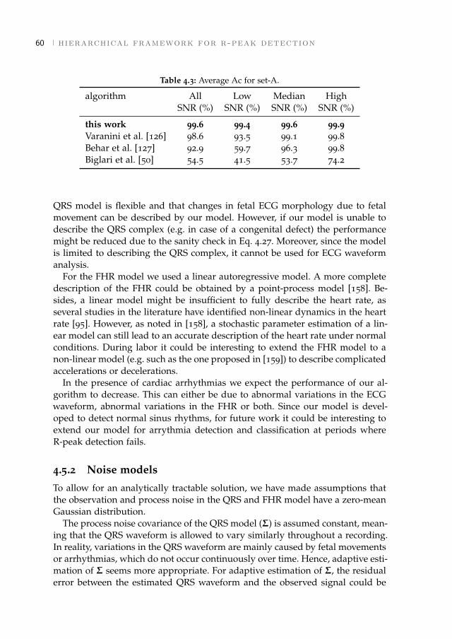
60 hierarchical framework for r-peak detection
Table 4.3: Average Ac for set-A.
algorithm All Low Median HighSNR (%) SNR (%) SNR (%) SNR (%)
this work 99.6 99.4 99.6 99.9Varanini et al. [126] 98.6 93.5 99.1 99.8Behar et al. [127] 92.9 59.7 96.3 99.8Biglari et al. [50] 54.5 41.5 53.7 74.2
QRS model is flexible and that changes in fetal ECG morphology due to fetalmovement can be described by our model. However, if our model is unable todescribe the QRS complex (e.g. in case of a congenital defect) the performancemight be reduced due to the sanity check in Eq. 4.27. Moreover, since the modelis limited to describing the QRS complex, it cannot be used for ECG waveformanalysis.
For the FHR model we used a linear autoregressive model. A more completedescription of the FHR could be obtained by a point-process model [158]. Be-sides, a linear model might be insufficient to fully describe the heart rate, asseveral studies in the literature have identified non-linear dynamics in the heartrate [95]. However, as noted in [158], a stochastic parameter estimation of a lin-ear model can still lead to an accurate description of the heart rate under normalconditions. During labor it could be interesting to extend the FHR model to anon-linear model (e.g. such as the one proposed in [159]) to describe complicatedaccelerations or decelerations.
In the presence of cardiac arrhythmias we expect the performance of our al-gorithm to decrease. This can either be due to abnormal variations in the ECGwaveform, abnormal variations in the FHR or both. Since our model is devel-oped to detect normal sinus rhythms, for future work it could be interesting toextend our model for arrythmia detection and classification at periods whereR-peak detection fails.
4.5.2 Noise models
To allow for an analytically tractable solution, we have made assumptions thatthe observation and process noise in the QRS and FHR model have a zero-meanGaussian distribution.
The process noise covariance of the QRS model (Σ) is assumed constant, mean-ing that the QRS waveform is allowed to vary similarly throughout a recording.In reality, variations in the QRS waveform are mainly caused by fetal movementsor arrhythmias, which do not occur continuously over time. Hence, adaptive esti-mation of Σ seems more appropriate. For adaptive estimation of Σ, the residualerror between the estimated QRS waveform and the observed signal could be
[ March 26, 2018 at 22:26 – classicthesis version 4.2 ]

4.5 discussion 61
used (similar to the method used for estimating the process noise of the FHRmodel). However, because the estimated QRS waveform is also used to identifymis-detections through Eq. 4.27, this approach reduces the performance. Despitehaving a fixed process noise covariance, the QRS model is still capable to adaptin case of fetal movement, as shown in Fig. 4.5.
For the estimation of the observation noise covariance of the QRS model (Λ),we assumed the observation noise to be uncorrelated. However, also correlatedphysiological noise (e.g. muscle activity) is described by the observation noiseof the QRS model. Although a whitening filter could be implemented as a pre-processing step, it is not straightforward to develop such a whitening filter forECG recordings since the correlation in the signal varies over time. In [142], itwas shown that even in case the observation noise is not white the Kalman filterprovides the optimal mean squared error solution.
For estimation of the process noise of the FHR model (Q), the observationnoise R plays an important role. If the value of R is overestimated, the pro-cess noise will be underestimated and the FHR model becomes less capable atadapting its model parameters to dynamical FHR variations that are caused bychanges in autonomic regulation. On the other hand, underestimating R leads tooverestimation of the process noise and overfitting of the parameter estimation.For future work it might be interesting to estimate R dynamically.
4.5.3 R-peak detection
New R-peaks are detected as the MAP estimate for the state-space model inEq. 4.6. The log-posterior is the sum of the estimation of the QRS and FHRmodel, weighted by the uncertainties in the respective models. If the quality ofthe recorded signal is high, the QRS model dominates the posterior distribution,as is shown in Fig. 4.6a. Conversely, if the signal quality is poor, the FHR modeldominates the posterior distribution, as is shown in Fig. 4.6b.
An MAP solution for R-peak detection was also proposed in [160]. However,the model that is used in [160] is designed for fiber-optic signals, from which itis not possible to detect the actual R-peaks locations due to differences in timingbetween audible and electrical activity of the heart. In [160], different detectionmethods are combined in an MAP estimate of the (ECG) R-peak location, thataccounts for the delays and uncertainties in each of the methods with respect totrue R-peak locations. This multimethod approach is not required in our case,because we measure the ECG and can detect actual R-peak locations.
In Fig. 4.7 an example is shown where ICA is unable to separate the fetalECG information in a single IC. In this example the SNR of the IC’s varies overtime, which reduces performance for algorithms that detect R-peaks on individ-ual channels, as demonstrated in Fig. 4.7a. In the multichannel extension of ourmodel all channels are used for R-peak detection, which improves the perfor-mance in case of varying SNR conditions (Fig. 4.7b).
[ March 26, 2018 at 22:26 – classicthesis version 4.2 ]
62 hierarchical framework for r-peak detection
The performance of our algorithm has been evaluated for set-A of the Chal-lenge. We compared performance of our algorithm to the performance of the al-gorithms of Varanini et al. [126], Behar et al. [127], and Biglari et al. [50]. Varaniniand Behar obtained the best scores for the Challenge. It should be noted that forset-B of the Challenge Andreotti et al. [125] and Lipponen et al. [128] achievedslightly better scores compared to Varanini and Behar in terms of FHR estima-tion. Since these algorithms were not publicly available we did not include themin our comparison.
Highest overall Ac was achieved by our algorithm (99.6%). The lowest perfor-mance was obtained by the algorithm of Biglari (54.5% overall Ac). Reasons forthe relatively low performance of the algorithm of Biglari could be that Biglariuses fixed templates for R-peak detection and that R-peaks are detected on theindividual channels. The algorithms of both Varanini and Behar achieved goodoverall Ac (98.6% and 92.9%, respectively). However, from Tabel 4.3 it becomesclear that the performance of these algorithms is reduced for low SNR conditions(93.5% for Varanini and 59.7% for Behar). In contrast, our algorithm achieved99.4% for the recordings with low SNR, indicating that our algorithm workswell even for low SNR conditions.
4.6 ConclusionIn this study, a hierarchical Bayesian framework was developed for fetal R-peakdetection. The developed method combines predictive models of the ECG wave-form and heart rate, and can be used for multichannel recordings. The developedmethod outperforms other methods that have been proposed in the literature interms of detection accuracy.
[ March 26, 2018 at 22:26 – classicthesis version 4.2 ]
PART II
Interpretation of fetal heart rate variabilityPART II
Interpretation of fetal heart rate variability
[ March 5, 2018 at 21:28 – classicthesis version 4.2 ]
[ March 26, 2018 at 22:26 – classicthesis version 4.2 ]

[ March 26, 2018 at 22:26 – classicthesis version 4.2 ]
5 U S I N G U T E R I N E A C T I V I T Y T O I M P R O V E F E TA LH RV A N A LY S I S F O R D E T E C T I O N O F A S P H Y X I AD U R I N G L A B O R
Abstract - During labor, uterine contractions can cause temporary oxygen deficiency forthe fetus. In case of severe and prolonged oxygen deficiency this can lead to asphyxia. Thecurrently used technique for detection of asphyxia, cardiotocography (CTG), suffers froma low specificity. Recent studies suggest that analysis of fetal heart rate variability (HRV)in addition to CTG can provide information on fetal distress. However, interpretation offetal HRV during labor is difficult due to the influence of uterine contractions on fetalHRV. The aim of this study is therefore to investigate whether HRV features differ duringcontraction and rest periods, and whether these differences can improve the detection ofasphyxia. To this end, a case-control study was performed, using 14 cases with asphyxiathat were matched with 14 healthy fetuses. We did not find significant differences forindividual HRV features when calculated over the fetal heart rate without separatingcontractions and rest periods (p > 0.30 for all HRV features). Separating contractionsfrom rest periods did result in a significant difference. In particular the ratio betweenHRV features calculated during and outside contractions can improve discriminationbetween fetuses with and without asphyxia (p < 0.04 for three out of four ratio HRVfeatures that were studied in this paper).1
1 This chapter is based on the paper published as Warmerdam G.J.J., Vullings R., Van Laar J.O.E.H., Vander Hout-Van der Jagt M.B., Bergmans J.W.M., Schmitt L., Oei S.G., "Using uterine activity to improvefetal heart rate variability analysis for detection of asphyxia during labor", Phys. Meas. 2016, 37: 387-400.
[ March 26, 2018 at 22:26 – classicthesis version 4.2 ]
66 uterine activity and fetal heart rate variability
5.1 IntroductionDuring labor, uterine contractions can cause temporary oxygen deficiency forthe fetus. Although a fetus is generally well-equipped to handle brief periodsof oxygen deficiency, if oxygen deficiency is severe and prolonged it can resultin asphyxia which is associated with neonatal morbidity and mortality [2]. It istherefore important that clinicians can timely intervene before asphyxia devel-ops.
Currently, cardiotocography (CTG) is the most often used method for detec-tion of asphyxia. CTG simultaneously records the fetal heart rate (FHR) anduterine activity (UA). The CTG is interpreted visually, based on standardizedguidelines [161]. Despite these guidelines, CTG interpretation has a high inter-and intra-observer variability [10]. Furthermore, the specificity of CTG is low,leading to a high false alarm rate [9]. To reduce the number of unnecessary oper-ative deliveries, additional information is required when the CTG is abnormal.
Recent studies have shown interest in analysis of fetal heart rate variability(HRV) to aid in the detection of asphyxia [31, 32, 36–39]. Because variations inthe heart rate are regulated by the autonomic nervous system (ANS), variousHRV features have been developed that attempt to quantify different aspects ofthe cardiac autonomic regulation [30]. Most of these features have been devel-oped for adults, but they might also provide diagnostic information about fetaldistress. Note that HRV features are usually defined for the analysis of inter-beat interval (R-R interval) signals and HRV features should thus not be applieddirectly to the FHR signal in beats per minute (BPM). Instead FHR should berecalculated to R-R intervals first.
Reviews of HRV features can be found in [33, 37, 94, 95]. Features describingthe statistical properties of a FHR signal have been used in [34] and [36] for detec-tion of fetal asphyxia. In [31], spectral analysis was used to examine the effect offetal asphyxia on the regulation of the sympathetic and parasympathetic branchof the ANS. Since the sympathetic and parasympathetic nervous system controlthe heart rate in different frequency bands, spectral analysis is able to separateregulation by these two branches [29]. In [31] it was shown that for fetuses withasphyxia normalized low frequency power increased while normalized high fre-quency power decreased, indicating a predominance of sympathetic regulation.
Spectral analysis is based on a linear model to describe the relation betweenANS regulation and variations in the heart rate. Besides spectral analysis, otherHRV features have been developed that quantify variations that cannot be ex-plained by this linear model. FHR signals were analyzed using HRV featuresthat quantify the complexity in a time series in [36, 162–164]. Furthermore, frac-tal analysis has also been employed to describe the FHR signal during labor [38,165].
To improve the predictive capacity of HRV features, several studies have com-bined multiple HRV features by using classifiers such as support vector ma-chines [35, 37] or neural networks [39].
[ March 26, 2018 at 22:26 – classicthesis version 4.2 ]
5.2 methods 67
Despite these efforts, it remains difficult to interpret HRV features calculatedfrom a FHR signal during labor, since most HRV features have been developedfor adults. Unlike for adults, changes in the fetal cardiovascular system during la-bor cannot be controlled and they are strongly influenced by uterine contractions.There are several ways by which contractions can influence the fetal cardiovas-cular system [1]. The rise in external pressure can directly change the fetal bloodpressure, which activates a baroreceptor reflex. Contractions can also indirectlyinfluence the fetal cardiovascular system, by blocking the oxygen supply to thefetus (e.g. due to umbilical cord occlusion or reduced maternal blood flow tothe placenta), activating a chemoreceptor reflex. After a contraction, some timeis needed for the fetal blood gases to recover. In addition, labor can be dividedinto different stages and the influence of contractions on the fetus changes overtime. The first stage is a period of progressive cervical dilation, followed by thesecond stage of active pushing where the fetal head descends into the birth canal.As a result of this uncontrolled environment, HRV features are often calculatedover highly non-stationary FHR signals.
This is also indicated by [52] and [51], who showed that for healthy fetusesspectral power is significantly higher during contractions as compared to restperiods (i.e. the periods in between contractions). The increase in spectral powerindicates a capability of the ANS to react to uterine contractions. CalculatingHRV features over the entire FHR signal, without consideration of contractions,averages this effect over the rest periods.
The aim of this study was therefore to examine whether separating contrac-tions from rest periods can improve HRV analysis for the detection of asphyxiaduring labor. To this end, a case-control study was used to examine the value ofseveral conventional HRV features in discriminating between fetuses with andwithout asphyxia.
5.2 Methods
5.2.1 Data acquisition
Data for this study was obtained at the Máxima Medical Center in Veldhovenand the University Medical Center in Utrecht over the period 2001 to 2008. Allregistrations were recorded on a Neoventa STAN® system. We used beat-to-beatFHR signals that were recorded using a scalp electrode. The UA was measuredeither via a tocodynamometer or via an intra-uterine pressure catheter (IUPC).
Registrations were included from healthy mothers who had an uncomplicatedpregnancy of at least 36 weeks of gestation and did not use any medication.Pregnancies complicated by intra-uterine growth restriction or fetal congenitalanomalies were excluded. Furthermore, we only included registrations with atleast 15 minutes of FHR signal during the second stage of labor. Contractionswere annotated by a clinical expert based on the UA trace, who was blinded tothe FHR signal and any other patient or medical information, including the fetal
[ March 26, 2018 at 22:26 – classicthesis version 4.2 ]

68 uterine activity and fetal heart rate variability
Table 5.1: Clinical characteristics of included fetuses.
Clinical features fetuses without fetuses withasphyxia asphyxia
(cases n=14) (cases n=14)
Gestational age (days) 284 ± 10 284 ± 9Birth weight (g) 3773 ± 587 3601 ± 4421-minute Apgar score 9 ± 1 7 ± 25-minute Apgar score 10 ± 0 8 ± 2Cord arterial pH 7.26 ± 0.06 6.99 ± 0.06Cord arterial base excess (mmol/l) −5 ± 2 −17 ± 3Length second stage of labor (min) 58 ± 27 71 ± 49Start before birth (min) 17 ± 3 25 ± 11
a Values are expressed as mean and standard deviation.
outcome. Only registrations with good quality UA trace were used, defined asregistrations where the expert was able to distinguish the contractions.
Fetal outcome was based on the umbilical arterial acid-base status; a pH above7.20 was defined as healthy, and a pH below 7.05 and base excess below -12 asasphyxia [1, 22]. Out of the 1232 registrations, 14 cases of fetuses with asphyxiaremained for analysis, that were matched with the registration of 14 healthyfetuses that were randomly selected from the available data. Besides the inclu-sion criteria mentioned in the previous paragraph, no further criteria were usedto match the two populations. The main clinical characteristics of the includedfetuses is shown in Table 6.1.
5.2.2 Signal processing
HRV features were calculated on R-R interval signals that were extracted fromNeoventa STAN® recordings. Since beat-to-beat R-R intervals can only be deter-mined when a heartbeat occurs, the R-R intervals are not equidistantly sampled.To obtain an equidistantly sampled signal, a sample and hold technique wasused [166]. To obtain a smooth function, the resulting signal was convolutedwith a square function of width 0.5 s and sampled at a rate of 4 Hz.
When the difference between two successive R-R intervals was more than 25BPM or more than 200ms, both R-R intervals were considered as artifacts. Thereason we also used 200 ms as criterion is that, in case of very low heart rate,it can occur that the difference between successive beats is more than 200 msbut less than 25 BPM. Artifacts were corrected by linear interpolation from theprevious correct R-R interval to a new segment of 5 consecutive R-R intervalswith less than 10 BPM difference between them [35]. For each registration, we
[ March 26, 2018 at 22:26 – classicthesis version 4.2 ]
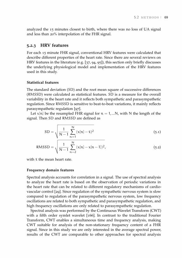
5.2 methods 69
analyzed the 15 minutes closest to birth, where there was no loss of UA signaland less than 20% interpolation of the FHR signal.
5.2.3 HRV features
For each 15 minute FHR signal, conventional HRV features were calculated thatdescribe different properties of the heart rate. Since there are several reviews onHRV features in the literature (e.g. [37, 94, 95]), this section only briefly discussesthe underlying physiological model and implementation of the HRV featuresused in this study.
Statistical features
The standard deviation (SD) and the root mean square of successive differences(RMSSD) were calculated as statistical features. SD is a measure for the overallvariability in the heart rate and it reflects both sympathetic and parasympatheticregulation. Since RMSSD is sensitive to beat-to-beat variations, it mainly reflectsparasympathetic regulation [97].
Let x[n] be the resampled FHR signal for n = 1, ...N, with N the length of thesignal. Then SD and RMSSD are defined as
SD =
√√√√ 1
N− 1
N∑n=1
(x[n] − x)2 (5.1)
RMSSD =
√√√√ 1
N− 1
N∑n=2
(x[n] − x[n− 1])2, (5.2)
with x the mean heart rate.
Frequency domain features
Spectral analysis accounts for correlation in a signal. The use of spectral analysisto analyze the heart rate is based on the observation of periodic variations inthe heart rate that can be related to different regulatory mechanisms of cardio-vascular control [29]. Since regulation of the sympathetic nervous system is slowcompared to regulation of the parasympathetic nervous system, low frequencyoscillations are related to both sympathetic and parasympathetic regulation, andhigh frequency oscillations are only related to parasympathetic regulation.
Spectral analysis was performed by the Continuous Wavelet Transform (CWT)with a fifth order symlet wavelet [166]. In contrast to the traditional FourierTransform, CWT enables a simultaneous time and frequency analysis, makingCWT suitable for analysis of the non-stationary frequency content of a FHRsignal. Since in this study we are only interested in the average spectral power,results of the CWT are comparable to other approaches for spectral analysis
[ March 26, 2018 at 22:26 – classicthesis version 4.2 ]

70 uterine activity and fetal heart rate variability
that account for non-stationarity in a signal, such as the Short Term FourierTransform (STFT) used in [31] or the Welch method used in [36]. However, unlikeSTFT and Welch method, CWT allows for a multi-resolution time frequencyanalysis. Since artefact correction in the FHR signal mainly affects the higherfrequencies, having a higher time resolution for these frequencies will reducethe influence of artefact correction [166].
The CWT compares the FHR signal (x[n]) to an analyzing wavelet functionψ. A wavelet is defined as a mother wavelet function ψ[n], with a family ofscaled and time-shifted daughter wavelets ψ[n−τs ]. The CWT coefficients W[s, τ]can be obtained by continuously varying the scale parameter s and the positionparameter τ. For real discrete signals, as is the case for the FHR signal, W[s, τ]can be calculated according to
W[s, τ] =1√s
N∑n=1
x[n]ψ[n− τ
s]. (5.3)
To correct for the convolution of the beat-to-beat FHR signal with a squarefunction that was used for smoothing (as explained in section 5.2.2), W[s, τ] isfirst divided by the coefficients of the wavelet transform of this square function.From the corrected wavelet coefficients (W[s, τ]) the power at each time instantat a certain scale is calculated as
P[s, τ] =1
Cg
(W[s, τ]s
)2, (5.4)
where Cg is the admissibility constant. Since each daughter wavelet is relatedto a certain frequency, the total power in a frequency band is then calculated byintegrating P[s, τ] over the scales within that frequency band and by averagingover time. Note that unlike the discrete wavelet transform, the CWT is not lim-ited to a dyadic decomposition of a signal in the time-frequency plane [167]. Thescale is a continuous parameter and can be selected such that it corresponds toa frequency within a certain frequency band.
The low frequency band was set to 0.04-0.15 Hz and the high frequency bandto 0.4-1.5 Hz [31, 32]. Scales corresponding to the frequencies between thesebands (0.15-0.4 Hz) were discarded. Besides absolute low frequency power (LF)and high frequency power (HF), also normalized LF (LFn) and normalized HF(HFn) power are calculated by dividing LF and HF by the total power (TP, 0.04-1.5 Hz) [31].
The minimum length of FHR signal that is required to calculate LF (and TP)is determined by the largest wavelet of the LF band. Therefore, a segment of atleast 50 seconds is required to reliably calculate LF [168]. Similarly, calculationof normalized frequency powers (LFn and HFn) also requires 50 seconds.
[ March 26, 2018 at 22:26 – classicthesis version 4.2 ]
5.2 methods 71
Complexity features
Although spectral analysis provides information about regulation mechanismsof the cardiovascular system, variations in the heart rate often cannot be ex-plained by spectral analysis alone. Since many factors can cause blood pressurechanges (e.g. changes in external pressure or through chemoreceptor reflex),blood pressure often shows complicated and irregular fluctuations. Because ad-justing the heart rate is one of the main tools of the ANS to stabilize these bloodpressure fluctuations, also the heart rate can show complicated and irregularfluctuations. The occurrence of irregularities in the heart rate is therefore indica-tive of healthy blood pressure control by the ANS.
A measure that is often used to quantify the complexity of very short signalsin terms of randomness is Sample Entropy (SampEn) [99]. SampEn estimatesthe conditional probability that when patterns are similar for length m− 1, theywill also be similar for length m. This probability is small in case the heart rateis complex and large in case the heart rate is not complex.
To calculate SampEn, the FHR signal is divided vectors u of length m
u[i] = {x[i], x[i+ 1], ..., x[i+m− 1]}. (5.5)
Two vectors u[i] and u[j] are similar if the maximum distance between the el-ements of u[i] and u[j] is less than tolerance parameter r. Let us define Cmi [r]
as the number of vectors u[j] that are similar to u[i] (for j 6= i), normalized bythe total number vectors of length m. The probability (Φm) of finding similarvectors of length m is then calculated as the average of Cmi [r]
Φm[r] = (N−m+ 1)−1N−m+1∑i=1
Cmi [r]. (5.6)
SampEn is the natural logarithm of the conditional probability in the limitN→∞
SampEn[m, r] = limN→∞− ln
Φm+1[r]
Φm[r]. (5.7)
The embedding dimension m was set to m = 2 and the tolerance to r = 0.2SD,similar to [36, 37, 163]. For finite time series, SampEn can be approximatedreliably with N > 100 samples [99].
Fractal features
Besides examining how the heart rate is controlled at certain specific time scales(e.g. LF and HF band for spectral analysis), for adults, fluctuations in the heartrate show self-similarity on different time scales [\cite ]Goldberger2002. In thiscontext, self-similarity means that structure of the heart rate on long time scales
[ March 26, 2018 at 22:26 – classicthesis version 4.2 ]
72 uterine activity and fetal heart rate variability
is resembled at shorter time scales. Fractal analysis describes the scaling proper-ties of the heart rate. In [38], fractal analysis was used to investigate the scalingproperties of the FHR during labor.
In our study, the variability at different time scales is described by the scalingexponent α, which is obtained by Detrended Fluctuation Analysis (DFA) [169,170]. To calculate α, first an integrated version of the original time series is ob-tained:
y[k] =
k∑n=1
(x[n] − x). (5.8)
Next, y[k] is divided into equally spaced segments of length a and the lineartrend of each segment (ya[k]) is determined. The characteristic fluctuation F ateach scale a is computed as the root mean square (RMS) deviation between y[k]and its trend:
F[a] =
√√√√ 1
N
N∑k=1
(y[k] − ya[k])2. (5.9)
If a linear relation exists between log(F[a]) and log(a), the heart rate is said toshow self-similarity, such that variability at long time scales is related to variabil-ity at shorter time scales in a power-law fashion (F[a] ∼ aα). The slope α of therelation between log(F[a]) and log(a) characterizes the type of the time series(e.g. α = 0.5 for white noise and α = 1.5 for Brownian noise). Also note that α isrelated to the Hurst exponent used in [38] as H = α− 1 [171].
Similar to [38], α was computed over the scales ranging from 1 to 60 seconds,which corresponds to the physiological range of the baroreflex.
5.2.4 HRV analysis during contractions and rest periods
For calculation of HRV features during contractions and rest periods separately,the expert annotations of the contractions were used. To calculate HRV featuresduring contractions, values based on R-R intervals measured during rest pe-riods were excluded. Similarly, to calculate HRV features during rest periods,values based on R-R intervals measured during contractions were excluded. Inour study, we also considered the ratio between HRV features calculated duringcontractions and rest periods.
It is important to note that in the second stage of labor the duration of con-tractions and rest periods is often less than one minute. Since computation of LF,LFn, HFn, and α requires approximately one minute of consecutive FHR signal,we could not extract these HRV features during contractions and rest periodsseparately.
Our study of HRV features during contractions and rest periods was thuslimited to SD, RMSSD,HF, and SampEn. Besides calculating these HRV features
[ March 26, 2018 at 22:26 – classicthesis version 4.2 ]
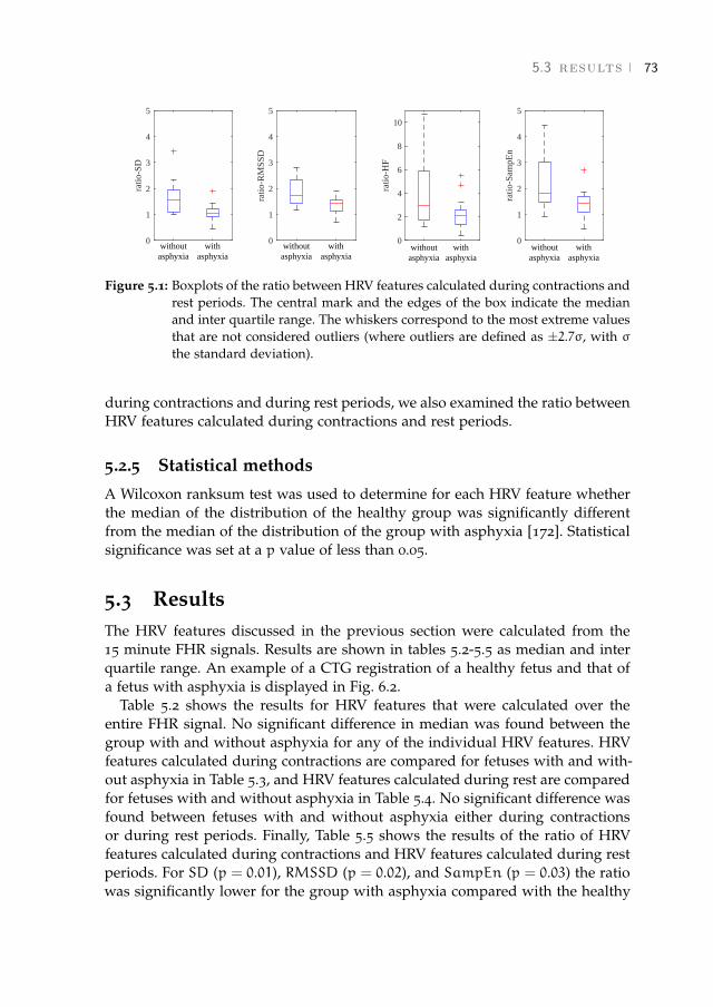
5.3 results 73
0
1
2
3
4
5
ratio
-SD
withoutasphyxia
withasphyxia
0
1
2
3
4
5
ratio
-RM
SSD
withoutasphyxia
withasphyxia
0
2
4
6
8
10
ratio
-HF
withoutasphyxia
withasphyxia
0
1
2
3
4
5
ratio
-Sam
pEn
withoutasphyxia
withasphyxia
Figure 5.1: Boxplots of the ratio between HRV features calculated during contractions andrest periods. The central mark and the edges of the box indicate the medianand inter quartile range. The whiskers correspond to the most extreme valuesthat are not considered outliers (where outliers are defined as ±2.7σ, with σthe standard deviation).
during contractions and during rest periods, we also examined the ratio betweenHRV features calculated during contractions and rest periods.
5.2.5 Statistical methods
A Wilcoxon ranksum test was used to determine for each HRV feature whetherthe median of the distribution of the healthy group was significantly differentfrom the median of the distribution of the group with asphyxia [172]. Statisticalsignificance was set at a p value of less than 0.05.
5.3 ResultsThe HRV features discussed in the previous section were calculated from the15 minute FHR signals. Results are shown in tables 5.2-5.5 as median and interquartile range. An example of a CTG registration of a healthy fetus and that ofa fetus with asphyxia is displayed in Fig. 6.2.
Table 5.2 shows the results for HRV features that were calculated over theentire FHR signal. No significant difference in median was found between thegroup with and without asphyxia for any of the individual HRV features. HRVfeatures calculated during contractions are compared for fetuses with and with-out asphyxia in Table 5.3, and HRV features calculated during rest are comparedfor fetuses with and without asphyxia in Table 5.4. No significant difference wasfound between fetuses with and without asphyxia either during contractionsor during rest periods. Finally, Table 5.5 shows the results of the ratio of HRVfeatures calculated during contractions and HRV features calculated during restperiods. For SD (p = 0.01), RMSSD (p = 0.02), and SampEn (p = 0.03) the ratiowas significantly lower for the group with asphyxia compared with the healthy
[ March 26, 2018 at 22:26 – classicthesis version 4.2 ]
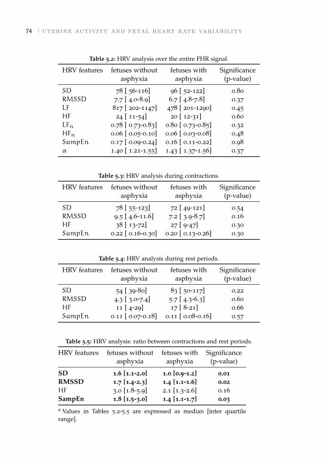
74 uterine activity and fetal heart rate variability
Table 5.2: HRV analysis over the entire FHR signal.
HRV features fetuses without fetuses with Significanceasphyxia asphyxia (p-value)
SD 78 [ 56-116] 96 [ 52-122] 0.80RMSSD 7.7 [ 4.0-8.9] 6.7 [ 4.8-7.8] 0.37LF 817 [ 202-1147] 478 [ 201-1290] 0.45HF 24 [ 11-54] 20 [ 12-31] 0.60LFn 0.78 [ 0.73-0.83] 0.80 [ 0.73-0.85] 0.32HFn 0.06 [ 0.05-0.10] 0.06 [ 0.03-0.08] 0.48SampEn 0.17 [ 0.09-0.24] 0.16 [ 0.11-0.22] 0.98α 1.40 [ 1.21-1.55] 1.43 [ 1.37-1.56] 0.37
Table 5.3: HRV analysis during contractions.
HRV features fetuses without fetuses with Significanceasphyxia asphyxia (p-value)
SD 78 [ 55-123] 72 [ 49-121] 0.54RMSSD 9.5 [ 4.6-11.6] 7.2 [ 3.9-8.7] 0.16HF 38 [ 13-72] 27 [ 9-47] 0.30SampEn 0.22 [ 0.16-0.30] 0.20 [ 0.13-0.26] 0.30
Table 5.4: HRV analysis during rest periods.
HRV features fetuses without fetuses with Significanceasphyxia asphyxia (p-value)
SD 54 [ 39-80] 83 [ 50-117] 0.22RMSSD 4.3 [ 3.0-7.4] 5.7 [ 4.3-6.3] 0.60HF 11 [ 4-29] 17 [ 8-21] 0.66SampEn 0.11 [ 0.07-0.18] 0.11 [ 0.08-0.16] 0.57
Table 5.5: HRV analysis: ratio between contractions and rest periods.
HRV features fetuses without fetuses with Significanceasphyxia asphyxia (p-value)
SD 1.6 [1.1-2.0] 1.0 [0.9-1.2] 0.01RMSSD 1.7 [1.4-2.3] 1.4 [1.1-1.6] 0.02HF 3.0 [1.8-5.9] 2.1 [1.3-2.6] 0.16SampEn 1.8 [1.5-3.0] 1.4 [1.1-1.7] 0.03a Values in Tables 5.2-5.5 are expressed as median [inter quartilerange].
[ March 26, 2018 at 22:26 – classicthesis version 4.2 ]

5.3 results 75
0 3 6 9 12 15
time (min)
0
25
50
75
100
UA
(m
mH
g)
50
100
150
200
FHR
(B
PM)
(a)
0 3 6 9 12 15
time (min)
0
25
50
75
100
UA
(m
mH
g)
50
100
150
200
FHR
(B
PM)
(b)
Figure 5.2: Example of a FHR signal of a healthy fetus (a) and a fetus with asphyxia (b).For the healthy fetus, the ratios between HRV features during contractionsand rest periods are: SD = 3.4, RMSSD = 2.8, HF = 10.5, and SampEn = 4.5.For the fetus with asphyxia, the ratios are: SD = 1.0, RMSSD = 1.6, HF = 2.1,and SampEn = 1.7.
group. Although the median ratio for HF was also lower for the group with as-phyxia, this difference was not significant. Complementary to results in Table5.5, the distributions of the ratio of HRV features are shown as boxplots in Fig.5.1.
[ March 26, 2018 at 22:26 – classicthesis version 4.2 ]
76 uterine activity and fetal heart rate variability
5.4 DiscussionThere are many factors that determine the response of the fetus to a temporalloss of oxygen caused by uterine contractions. Therefore, CTG registrations oftendisplay a large variety of complicated patterns, making it difficult to interpretthem. Automated analysis of fetal HRV attempts to support clinicians in theirinterpretation by providing additional quantitative information on the cardio-vascular system. However, existing HRV features have been mainly developedfor adults and do not account for the strong influence of uterine contractions onthe cardiovascular control. When calculating these HRV features over the entireFHR signal, the effect of contractions is averaged with rest periods. The goal ofthis study was to show that separating contractions from rest periods improvesHRV analysis for the detection of fetal asphyxia.
Despite the relatively large number of available registrations, only 14 caseswith pH below 7.05 could be included for the analysis. This is partly due to thelow incidence of asphyxia (between 0.6% [173] and 3.5% [174]), but also becauseof the strict inclusion criteria we used. We required a good quality UA trace, sothat the expert could clearly identify contractions. In clinical practice, however,it frequently occurs that the UA trace is of poor quality [175]. A potential solu-tion might be the use of electrohysterography for the registration of UA [176].Note that in our dataset the number of registrations that measured UA withtocodynamometer or with IUPC was the same for both the healthy group andthe group with asphyxia (10 with tocodynamometer and 4 with IUPC). Since weonly included registrations with good quality UA trace, we expect that the useof tocodynamometer or IUPC did not influence our results.
For some recordings we were unable to analyze the final minutes before birth,either due to loss of FHR signal or insufficient quality of UA trace (Table 6.1).As a result, segments for the healthy group were selected closer to birth thanfor the group with asphyxia. Because it has been reported that, in absence ofsudden catastrophic events, asphyxia in term fetuses develops within a period ofat least 90 minutes [177], we can assume that fetuses in the group with asphyxiawere already under more stressful conditions than fetuses in the healthy group.We expect the effect of asphyxia to increase as labor progresses and differencesbetween healthy fetuses and fetuses with asphyxia to be even more pronouncedduring the final minutes before birth.
5.4.1 HRV features over the entire FHR signal
We did not find a significant difference between the healthy group and the groupwith asphyxia for individual HRV features when calculated over the entire FHRsignal (Table 5.2). This could partly be explained by the small number of record-ings and large inter-patient variability of the HRV features.
For absolute LF and HF, our results are similar to the findings in [36] and[31], despite the different method they used for spectral analysis (Welch method
[ March 26, 2018 at 22:26 – classicthesis version 4.2 ]
5.4 discussion 77
and STFT respectively, versus CWT used in this study). Although in our studynormalized LF was higher for the group with asphyxia, in line with [31], thisdifference was not significant. Furthermore, in contrast to the findings in [36],SampEn was not statistically different. These differences in results obtainedin our study and [36] and [31], might be because [36] and [31] calculated theHRV features over short segments of FHR signal (5 minutes). As discussed in[36], HRV analysis could be more efficient when performed on shorter segments.However, we used longer segments because in shorter segments a bias could beintroduced due to an unbalance in the presence of contractions and rest peri-ods within the segment. The use of shorter segments can therefore lead to largeintra-patient variability of HRV features over time.
In our study also no difference was found between healthy fetuses and fetuseswith asphyxia for the scaling exponent α. Recently [165] showed promising re-sults calculating the scaling exponent using a wavelet based scattering transform.This might improve the fractal analysis.
5.4.2 HRV features during contractions and rest periods
Similar to [51] and [52], we found that for healthy fetuses HF was significantlyincreased during contractions with respect to rest periods (p = 0.01). This resulthas not been shown explicitly, but can be seen by comparing the left columnsof tables 5.3 and 5.4. The increase in HRV features during contractions relativeto the HRV features during rest periods indicates that a stronger cardiovascularcontrol is required to stabilize the blood pressure during contractions. The risein external pressure due to contractions can activate a combination of barorecep-tor and chemoreceptor reflexes, leading to relatively high HRV during contrac-tions. This finding was confirmed by the observed increase in RMSSD (p < 0.01)and SampEn (p < 0.01). In contrast to the results of the healthy group, for thegroup with asphyxia HRV features were not significantly different during con-tractions with respect to rest periods (all p > 0.12, obtained by comparing theright columns of Table 5.3 and 5.4).
Despite this increase in HRV features during contractions for the healthygroup, no significant difference was found when comparing HRV features ofthe healthy group to the group without asphyxia either during contractions orduring rest periods, as shown in tables 5.3 and 5.4 respectively. A possible rea-son why no significant difference was observed between the two groups (eitherduring contractions or during rest periods) might be the large inter-patient vari-ability in obtained values for the HRV features and the relatively small dataset.
5.4.3 HRV features: ratio between contractions and rest periods
When considering the ratio between HRV features calculated during contractionsand rest periods, SD, RMSSD, and SampEn were all significantly lower for thegroup with asphyxia than for the healthy group (Table 5.5). Also the ratio for
[ March 26, 2018 at 22:26 – classicthesis version 4.2 ]
78 uterine activity and fetal heart rate variability
HF was lower (as can be seen in Fig. 5.1), but this was not significant due to thelarge spread in the distribution.
For healthy fetuses, a high ratio of HRV features during contractions and restperiods might indicate a response of the fetal ANS to stabilize the cardiovascularsystem. On the one hand, during contractions HRV features are high because thefetus needs to adapt its cardiovascular system to changes in external pressure[51, 52]. On the other hand, during rest periods little cardiovascular control is re-quired because in the second stage of labor fetal movement is reduced [178]. Fur-thermore, after a contraction has ended, a healthy fetus has not suffered muchfrom indirect effect of contractions on the cardiovascular system (i.e. umbili-cal cord occlusion or reduced maternal blood flow). Therefore, healthy fetusesquickly recover from contractions and HRV features will be low during rest pe-riods. As a result, a high ratio is observed for HRV features during contractionsand rest periods. Note that if a fetus is not compromised by contractions, HRVfeatures will be similar during contractions and rest periods, leading to a lowratio rather than a high ratio. However, the case where a fetus does not suffer atall is relatively simple to recognize by a clinician based on the FHR signal (e.g.when there are no decelerations in the FHR trace).
Unlike healthy fetuses, a fetus with asphyxia is not able to adequately adaptits cardiovascular system during contractions. Therefore, HRV features duringcontractions are relatively low for fetuses with asphyxia compared to healthyfetuses (although not significant, as shown in Table 5.3). Even after a contrac-tion has ended, the oxygen concentration of the fetal blood is still low due toaforementioned indirect effects of contractions on the fetal cardiovascular sys-tem. The fetus thus also needs to adapt its cardiovascular system during restperiods, which can lead to decelerations that last until after contractions or evenstart after contractions have ended [1]. HRV features during rest are thus higherfor fetuses with asphyxia compared to healthy fetuses (although not significant,as shown in Table 5.4). As a result, the ratio of HRV features during contractionsand rest periods is lower for fetuses with asphyxia than for healthy fetuses.
An example of a registration of a fetus with and without asphyxia is shownin Fig. 6.2. For the healthy fetus, decelerations occur on top of contractions anda stable heart rate is observed during rest periods. The ratios of HRV featuresduring contractions and rest periods are therefore high (SD = 3.4, RMSSD =
2.8, HF = 10.5, and SampEn = 4.5). For the fetus with asphyxia, decelerationsare prolonged and last until after the contractions have ended. The ratios ofHRV features during contractions and rest periods are therefore low (SD = 1.0,RMSSD = 1.6, HF = 2.1, and SampEn = 1.7).
5.4.4 Future perspective
Our results are promising and show that distinguishing contractions from restperiods improves HRV analysis for detection of asphyxia. However, we only
[ March 26, 2018 at 22:26 – classicthesis version 4.2 ]

5.5 conclusion 79
used a small dataset. To determine the diagnostic value for clinical practice, fur-ther study is required using a larger dataset. Besides, we only examined theeffect on individual HRV features. In [35, 37, 39, 179], it was shown that combi-nations of multiple HRV features using classifiers can improve the detection rateof fetal asphyxia. It is therefore interesting to combine multiple HRV featurescalculated over the entire fetal heart signal with HRV features calculated duringcontractions and rest periods. Furthermore, it might also be interesting to mon-itor changes in HRV features over the course of labor as was done in [31, 165,180].
5.5 ConclusionAnalysis of fetal HRV provides information on fetal asphyxia. Results in ourstudy suggest that separating contractions and rest periods improves HRV anal-ysis for the detection of asphyxia during labor. In particular, using the ratiobetween HRV features calculated from contractions and rest periods improvesthe ability of the HRV features to discriminate between healthy fetuses and fe-tuses with asphyxia. Further studies are required to determine the diagnosticvalue in clinical practice.
[ March 26, 2018 at 22:26 – classicthesis version 4.2 ]

[ March 26, 2018 at 22:26 – classicthesis version 4.2 ]
6 D E T E C T I O N R AT E O F F E TA L D I S T R E S S U S I N GC O N T R A C T I O N - D E P E N D E N T F E TA L H E A RT R AT EVA R I A B I L I T Y A N A LY S I S
Abstract - Objective: Monitoring of the fetal condition during labor is currently per-formed by cardiotocography (CTG). Despite the use of CTG in clinical practice, CTGinterpretation suffers from a high inter- and intra-observer variability and a low speci-ficity. In addition to CTG, analysis of fetal heart rate variability (HRV) has been shownto provide information on fetal distress. However, fetal HRV can be strongly influencedby uterine contractions, particularly during the second stage of labor. Therefore, the aimof this study is to examine if distinguishing contractions from rest periods can improvethe detection rate of HRV features for fetal distress during the second stage of labor.Methods: We used a dataset of 100 recordings, containing 20 cases of fetuses with ad-verse outcome. The most informative HRV features were selected by a Genetic Algorithmand classification performance was evaluated using Support Vector Machines. Results:Classification performance of fetal heart rate segments closest to birth improved from ageometric mean of 70% to 79%. If the classifier was used to indicate fetal distress overtime, the geometric mean at 15 minutes before birth improved from 60% to 72%. Conclu-sion and significance: Our results show that combining contraction-dependent HRVfeatures with HRV features calculated over the entire fetal heart rate signal improves thedetection rate of fetal distress.1
1 This chapter is based on the paper published as Warmerdam, G.J.J., Vullings R., Van Laar J.O.E.H.,Van der Hout-Van der Jagt B., Bergmans J.W.M., Schmitt L., Oei S.G., "Detection rate of fetal distressusing contraction-dependent fetal heart rate variability analysis", in Phys. Meas., 2018.
[ March 26, 2018 at 22:26 – classicthesis version 4.2 ]
82 contraction-dependent fetal heart rate variability analysis
6.1 IntroductionThe introduction of cardiotocography (CTG) in the 1960s, has enabled continu-ous monitoring of the fetal heart rate (FHR) and uterine contractions. In currentobstetric units, CTG has become the worldwide standard for detection of fetaldistress during labor. However, the CTG is interpreted visually and the inter-and intra-observer variability is high [10]. Furthermore, despite a high sensi-tivity of CTG interpretation, the specificity is poor [7]. As a result of the lowspecificity, the rate of unnecessary operative interventions has increased sincethe introduction of CTG in the clinic [9]. To detect if the fetus is in distress,additional information is therefore often required when the CTG is abnormal.
In recent studies, analysis of fetal heart rate variability (HRV) has been shownto provide information on fetal distress [31, 32, 36–39, 179, 181]. Since the auto-nomic nervous system (ANS) regulates the heart rate, variations in the heart ratereveal autonomic regulation and might indirectly provide information on fetaldistress. To quantify changes in HRV, several features have been developed inthe literature that describe different aspects of HRV. For overviews of the mostcommonly used HRV features the reader is referred to [95] or [94].
Most HRV features have been developed and validated for adults in controlledexperiments. However, unlike for adults, changes in the exterior of the fetus can-not be controlled during labor. Uterine contractions can lead to a temporaryreduction of oxygen supply to the fetus (e.g. due to umbilical cord occlusionor reduced maternal placental blood flow). Besides, uterine contractions cancause large fluctuations in the intrauterine pressure, directly influencing the fe-tal cardiovascular system. As labor progresses into a stage of active pushing, thestrength and influence of contractions increases.
In [51] and [52], it was shown for healthy fetuses that HRV was significantlyhigher during contractions as compared to rest periods (i.e. the period in be-tween contractions). Moreover, [180] used an input-output model to describe therelation between the uterine activity (UA) and FHR signal, and showed that fea-tures extracted from this model provided information about fetal distress. Thechange in FHR during contractions could indicate a healthy response of the fetalANS to stabilize the cardiovascular system. In a recent study we showed that thedifferences between HRV features during contractions and rest might be used toimprove the detection of fetal distress [181].
In [35, 37, 39, 179] it was shown that the detection of fetal distress can beimproved by classifying combinations of multiple HRV features. Therefore, inthis paper we examine whether the detection of fetal distress can be improvedby combining HRV features that were calculated over the entire heart rate withHRV features that were calculated separately during contractions and duringrest periods. To determine the most informative subset of HRV features, bothwith and without the additional contraction-dependent HRV features, we useda Genetic Algorithm (GA) [182]. Furthermore, the classification performance of
[ March 26, 2018 at 22:26 – classicthesis version 4.2 ]

6.2 methods 83
Pre-processing
Train classifier
Feature selection
HRV analysis
Validation over time
Initialize random population
Selection fitness value
New population
Cross overMutation
Check stopping criteria
Yes
Elite
No
Genetic Algorithm (GA)
Figure 6.1: Flowchart of signal processing.
these subsets for detection of fetal distress was evaluated over time, using Sup-port Vector Machines (DSPs) [183].
The rest of this paper is organized as follows; Section 6.2.1 discusses the dataacquisition and pre-processing. In Sections 6.2.2 and 6.2.3 we summarize theimplementation of the used HRV features. Feature selection, classification, andvalidation are explained in Sections 6.2.4-6.2.6. Results and discussion are pre-sented in Sections 6.3 and 6.4.
6.2 MethodsThis section describes the different HRV features, feature selection, and the clas-sification that was used in this paper. The overall classification procedure is pre-sented in Fig. 6.1.
6.2.1 Data acquisition and pre-processing
We used FHR and UA signals that were recorded on a Neoventa STAN® (Möl-ndal, Sweden) in the Máxima Medical Center in Veldhoven, the University Med-ical Center in Utrecht, and registrations collected in Sweden in the context ofSTAN evaluation over the period 2001-2008. Registrations of at least 36 weeksof gestation were included. Pregnancies complicated by intra-uterine growth re-striction, fever, fetal congenital anomalies, or use of ritodrine were excluded. Weused beat-to-beat FHR signals that were recorded by a scalp electrode. UA wasrecorded with either a tocodynamometer or intra-uterine pressure catheter. Con-tractions were annotated by a clinical expert that had no knowledge of the FHRsignal or fetal outcome.
Because the beat-to-beat R-R intervals are determined when a heartbeat occurs,the R-R intervals are not equidistantly sampled. We used linear interpolation toobtain an equidistantly sampled FHR signal, sampled at a rate of 4 Hz. If an R-R
[ March 26, 2018 at 22:26 – classicthesis version 4.2 ]

84 contraction-dependent fetal heart rate variability analysis
Table 6.1: Clinical characteristics of included fetuses.
Clinical features healthy fetuses fetuses with(cases n=80) adverse outcome
(cases n=20)
Gestational age (days) 280 ± 10 283 ± 8Birth weight (g) 3551 ± 471 3560 ± 4671-minute Apgar score 8.6 ± 1.1 6.3 ± 2.05-minute Apgar score 9.5 ± 0.5 7.8 ± 2.0Cord arterial pH 7.25 ± 0.03 7.00 ± 0.04Cord arterial base excess (mmol/l) −5.8 ± 2.3 −16.0 ± 2.2Length second stage of labor (min) 58 ± 24 62 ± 24
a Values are expressed as mean and standard deviation.
interval changed by more than 25 BPM or more than 200 ms with respect to theadjacent R-R interval, the R-R interval was considered an artifact. Artifacts werecorrected by linear interpolation.
Each registration was divided into segments of 10 minutes, with five minuteoverlap. If a segment contained less than 20% loss of FHR signal and at leastannotation of two contractions and two rest periods, the segment was used forfurther analysis. We only included FHR signal during the second stage of labor(stage of active pushing), since during this stage contractions have a strong effecton the fetus. Besides, because we expect that the effects of oxygen deficiency in-crease as labor progresses, we only considered FHR segments up to maximally45 minutes before birth. Since we are also interested in the classification per-formance over time, only registrations were included with at least 3 usable 10minute segments within the final 45 minutes before birth.
The fetal outcome was based on the umbilical arterial acid-base state. Adverseoutcome was defined as a pH below 7.05 and base excess below -12 mmol/l, andhealthy as a pH above 7.20 [1]. Out of 1232 registrations, our dataset contained44 cases with adverse outcome. Of these 44 cases, 6 cases were excluded due toeither intra-uterine growth restriction, fever, fetal congenital anomalies, or usedof ritodrine. Another 6 had to be excluded because no information was availableon the onset of the second stage of labor. Of the remaining 32 cases, 20 cases hadsufficient quality FHR and UA signal, and were used for further analysis. The20 cases with adverse outcome were matched with 80 healthy cases (1-to-4 ratiobetween the size of both groups). We have attempted to match the prevalenceof certain medications that can cross the placenta and influence fetal HRV (e.g.anti-hypertensives or pain killers) in accordance with the difference in size of thetwo groups. The main clinical characteristics of the included fetuses is shown inTable 6.1.
[ March 26, 2018 at 22:26 – classicthesis version 4.2 ]
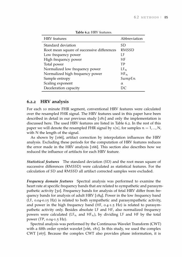
6.2 methods 85
Table 6.2: HRV features.
HRV features Abbreviation
Standard deviation SD
Root mean square of successive differences RMSSD
Low frequency power LF
High frequency power HF
Total power TP
Normalized low frequency power LFnNormalized high frequency power HFnSample entropy SampEn
Scaling exponent α
Deceleration capacity DC
6.2.2 HRV analysis
For each 10 minute FHR segment, conventional HRV features were calculatedover the resampled FHR signal. The HRV features used in this paper have beendescribed in detail in our previous study [181] and only the implementation isdiscussed here. The used HRV features are listed in Table 6.2. In the rest of thispaper we will denote the resampled FHR signal by x[n], for samples n = 1, ...,N,with N the length of the signal.
As shown by [166], artifact correction by interpolation influences the HRVanalysis. Excluding these periods for the computation of HRV features reducesthe error made in the HRV analysis [166]. This section also describes how wereduced the influence of artifacts for each HRV feature.
Statistical features The standard deviation (SD) and the root mean square ofsuccessive differences (RMSSD) were calculated as statistical features. For thecalculation of SD and RMSSD all artifact corrected samples were excluded.
Frequency domain features Spectral analysis was performed to examine theheart rate at specific frequency bands that are related to sympathetic and parasym-pathetic activity [30]. Frequency bands for analysis of fetal HRV differ from fre-quency bands for analysis of adult HRV [184]. Power in the low frequency band(LF, 0.04-0.15 Hz) is related to both sympathetic and parasympathetic activity,and power in the high frequency band (HF, 0.4-1.5 Hz) is related to parasym-pathetic activity only. Besides absolute LF and HF, also normalized frequencypowers were calculated (LFn and HFn), by dividing LF and HF by the totalpower (TP, 0.04-1.5 Hz).
Spectral analysis was performed by the Continuous Wavelet Transform (CWT)with a fifth order symlet wavelet [166, 181]. In this study, we used the complexCWT [167]. Because the complex CWT also provides phase information, it is
[ March 26, 2018 at 22:26 – classicthesis version 4.2 ]

86 contraction-dependent fetal heart rate variability analysis
possible to calculate the spectral power at each sample, leading to more reliablecalculation of LFn and HFn. Note that resampling of the beat-to-beat FHR signalto an equidistant signal may cause some distortion of the spectral analysis [185].Yet, we expect that the influence of this distortion on the outcome is limited sinceresampling was performed for all registrations.
CWT compares x[n] to a family of analyzing wavelet functions ψ[n−τs ], wheres is a scaling parameter and τ the position parameter of the wavelet. The CWTcoefficients W[s, τ] can be obtained by varying the scale parameter s and theposition parameter τ. The power at each time instant and scale is proportional tothe square of the CWT coefficients. The total power in a frequency band is thencalculated by integrating the power over the scales within the frequency band ofinterest and averaging over time.
Each wavelet ψ[n−τs ] has a support width that is related to the scaling param-eter s. Similar to [166], we considered one-third of support width of ψ[n−τs ] asthe effective support width. A CWT coefficient was excluded for the calculationof HF if one or more samples within the effective support width was artifactcorrected. To calculate LF, we excluded CWT coefficients when more than fiveseconds of consecutive FHR signal was artifact corrected within the effectivesupport width.
Complexity features The presence of irregularities in the heart rate is seen ashealthy blood pressure control by the ANS. Complexity in short time signals canbe quantified by Sample Entropy (SampEn) [99]. To calculate SampEn, the FHRis divided into vectors u[i] = {x[i], x[i+ 1], ..., x[i+m− 1]}. SampEn estimates theconditional probability that if patterns are similar for lengthm− 1, they will alsobe similar for length m. A tolerance parameter r is used to define a threshold forsimilarity between two patterns. We excluded vectors u[i] from the calculationof SampEn if any of the samples {i, i + 1, ..., i +m − 1} was artifact corrected.Similar to [36], [37] and [181], the length of the vectors was set to m = 2 and thetolerance to r = 0.2SD.
Fractal features To describe the scaling properties of HRV over different timescales, we used scaling exponent α, which is obtained from Detrended Fluctu-ation Analysis (DFA) [170]. To calculate α, first the cumulative sum y[n] of theFHR signal is obtained. Next, y[n] is divided into equally spaced segments oflength a and the linear trend of each segment (ya[n]) is determined. The charac-teristic fluctuation F at each scale a is computed as the root mean square (RMS)deviation between y[n] and its trend ya[n].
The scaling exponent α is given by the slope of the relation between log(F[a])and log(a). Similar to [38], α was computed over the scales ranging from 1 to 60seconds, which corresponds to the physiological range of the baroreflex.
Artifact corrected samples are excluded from the calculation of the linear trendya[n] and the characteristic fluctuation F. Moreover, if the percentage of artifactcorrection within a segment of length a is more than 20%, it is excluded entirely.
[ March 26, 2018 at 22:26 – classicthesis version 4.2 ]
6.2 methods 87
Phase rectified signal averaging In addition to the HRV features that were in-cluded in our previous study [181] and have been described above, we also usedPhase Rectified Signal Averaging (PRSA). PRSA has shown promising resultsfor the detection of fetal distress [186] and [179]. The basic idea of PRSA is toaccount for non-stationarities in the heart rate by aligning heart rate segmentsbased on predefined events, called anchor points (ν). For analysis of the heartrate, anchor points are typically defined as decelerations and accelerations inthe heart rate, and PRSA quantifies the average response to a deceleration (thedeceleration capacity, DC) or acceleration (the acceleration capacity, AC). It wasshown by [186] thatDC and AC are highly correlated and that their performancefor detection of fetal distress is similar. Therefore, we only included DC in ouranalysis.
PRSA depends on two parameters: a filter parameter T and a window parame-ter L [187]. Similar to [186] we used T = 5 and L = 45. Artifact corrected sampleswere not used as anchor points. Moreover, when there was more than 20% arti-fact correction within a window ν± L, the anchor point ν was also excluded.
6.2.3 Contraction-dependent HRV features
In addition to calculating HRV features over the entire FHR signal, we also cal-culated HRV features separately during contractions and rest periods. Using theexpert annotations, the rest period was defined as the period in between twocontractions. No contraction or rest period was defined if the length of a con-traction or the time between contractions was less than 20 seconds. Note thatthe fetus typically requires some recovery time directly after a contraction, buthas enough time to recover before a new contraction. Therefore, if the time be-tween two contractions was more than one minute, we only considered the finalminute preceding the second contraction as rest period. In Fig. 6.2 an exampleis shown of an FHR signal that is recorded during contractions and during restperiods.
HRV features during contractions were based on R-R intervals that wererecorded during contractions (denoted as featureuc). Similarly, HRV featuresduring rest periods were based on R-R intervals that were recorded during restperiods (denoted as featurerest). Also the ratio between HRV features calcu-lated during contractions and during rest was included (denoted as featureratio =
featureuc/featurerest), as the ratios have shown promising results in our pre-vious studies [181]. Because the time between contractions or the length of thecontractions was often less than one minute, we could not calculate LF, LFn, HFn,α and DC separately during contractions and during rest periods. Our analysisof contraction-dependent HRV features was therefore limited to SD, RMSSD,HF, and SampEn.
In total, 22 HRV features were used: 10 calculated over the entire FHR, 4 dur-ing rest, 4 during contractions, and 4 ratio features, as presented in Table 6.3.
[ March 26, 2018 at 22:26 – classicthesis version 4.2 ]

88 contraction-dependent fetal heart rate variability analysis
0 2.5 5 7.5 10
time (min)
0
25
50
75
100
UA
(m
mH
g)
50
100
150
200FH
R (
BPM
)
Figure 6.2: Example of an FHR (upper graph) and UA signal (bottom graph) of healthyfetus. Black lines are rest periods and gray lines contractions.
Table 6.3: HRV feature sets.
Feature set HRV features
S1 ∈ R10 SD, RMSSD, LF, HF, TP, LFn, HFn,SampEn, α, DC
S2 ∈ R12 SDuc, RMSSDuc, HFuc, SampEnucSDrest, RMSSDrest, HFrest, SampEnrestSDratio, RMSSDratio, HFratio, SampEnratio
S3 ∈ R22 S1 ∪ S2
We defined HRV feature set S1 ∈ R10 as the set of HRV features that are calcu-lated over the entire FHR, without distinguishing contractions and rest periods.The set of HRV features that contain the contraction-dependent HRV features isdefined as S2 ∈ R12. The set of HRV features that contains both HRV featuresthat are calculated over the entire FHR signal and contraction-dependent HRVfeatures is defined as S3 = S1 ∪ S2.
6.2.4 Feature selection
In [188] it was shown that many HRV features that are described in Section 6.2.2are correlated and might therefore contain redundant information. Besides, ourdataset is relatively small, with only 20 cases of fetuses with adverse outcome.As a consequence, there is a risk of overfitting when too many HRV features areused for classification. Therefore, we used a GA to select the best combinationof HRV features. GA has the advantage that it can effectively explore the entire
[ March 26, 2018 at 22:26 – classicthesis version 4.2 ]

6.2 methods 89
Table 6.4: GA settings.
Parameter Value
Population size 100Number of elite children 2Crossover fraction 80%Mutation function single pointfitness value SVM performancefitness function rankGenotype selection roulette systemMaximum number of features in genotype 5Maximum iterations with same fitness value 10Maximum iterations 200
feature space, without running through all possible combinations of features andit has successfully been used for detection of fetal distress by [179].
A schematic overview of GA is presented on the right side of Fig. 6.1. GA itera-tively creates populations of candidate feature subsets (genotypes) by randomlycombining and mutating genotypes of the population in a previous iteration, un-til certain convergence criteria are reached. In each iteration, the genotypes of thecurrent population are scored by a fitness function. Genotypes are then selectedat random to generate a new population with a probability that is proportionalto their fitness value. Each new population consists of elite children (best per-forming genotypes that are guaranteed to survive to the next iteration), childrenthat are produced by random mutations of a single genotype, and children thatare produced by random crossover between pairs of genotypes.
For the implementation of GA, we used ga from the standard Global Optimiza-tion Toolbox of Matlab® (The Mathworks, Inc. Natick, MA). As fitness function,we used the performance of an SVM classifier, which is explained in Section 6.2.5.Based on the ranking in fitness value, genotypes are selected using a roulette sys-tem [182]. Genotypes with equal scores were given equal rank and only the best50% was used to generate the next population. Similar to [179], the populationsize was set to 100, two elite children were used, and the crossover fraction wasset to 80%. The remaining 20% for the new population was obtained by singlepoint mutation. If two equal genotypes were selected for crossover, single pointmutation is used instead to generate the child. To prevent GA from reaching alocal minimum with a relatively large number of selected features, the numberof selected features of a genotype was restricted to a maximum of five features.The GA was terminated if the best fitness value of the population did not im-prove for 10 iterations or in case 200 iterations were done. The settings for GAare summarized in Table 6.4.
[ March 26, 2018 at 22:26 – classicthesis version 4.2 ]
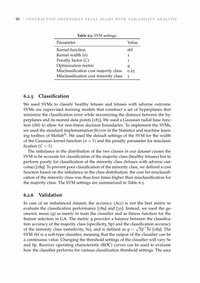
90 contraction-dependent fetal heart rate variability analysis
Table 6.5: SVM settings.
Parameter Value
Kernel function rbfKernel width (σ) 1Penalty factor (C) 1Optimization metric g
Misclassification cost majority class 0.25Misclassification cost minority class 1
6.2.5 Classification
We used SVMs to classify healthy fetuses and fetuses with adverse outcome.SVMs are supervised learning models that construct a set of hyperplanes thatminimize the classification error while maximizing the distance between the hy-perplanes and its nearest data points [183]. We used a Gaussian radial base func-tion (rbf) to allow for non-linear decision boundaries. To implement the SVMs,we used the standard implementation fitcsvm in the Statistics and machine learn-ing toolbox of Matlab®. We used the default settings of the SVM for the widthof the Gaussian kernel function (σ = 1) and the penalty parameter for misclassi-fication (C = 1).
The imbalance in the distribution of the two classes in our dataset causes theSVM to be accurate for classification of the majority class (healthy fetuses) but toperform poorly for classification of the minority class (fetuses with adverse out-come) [189]. To prevent poor classification of the minority class, we defined a costfunction based on the imbalance in the class distribution: the cost for misclassifi-cation of the minority class was thus four times higher than misclassification forthe majority class. The SVM settings are summarized in Table 6.5.
6.2.6 Validation
In case of an imbalanced dataset, the accuracy (Acc) is not the best metric toevaluate the classification performance [189] and [35]. Instead, we used the ge-ometric mean (g) as metric to train the classifier and as fitness function for thefeature selection in GA. The metric g provides a balance between the classifica-tion accuracy of the majority class (specificity, Sp) and the classification accuracyof the minority class (sensitivity, Se), and is defined as g =
√Sp · Se [189]. The
SVM rbf is a soft-type classifier, meaning that the output of the classifier can bea continuous value. Changing the threshold settings of the classifier will vary Seand Sp. Receiver operating characteristic (ROC) curves can be used to evaluatehow the classifier performs for various classification threshold settings. The area
[ March 26, 2018 at 22:26 – classicthesis version 4.2 ]
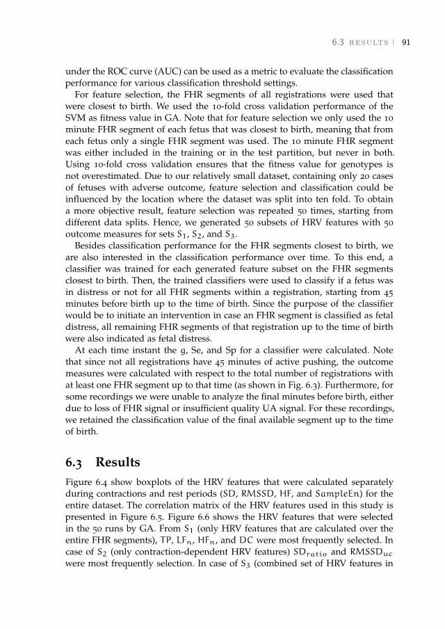
6.3 results 91
under the ROC curve (AUC) can be used as a metric to evaluate the classificationperformance for various classification threshold settings.
For feature selection, the FHR segments of all registrations were used thatwere closest to birth. We used the 10-fold cross validation performance of theSVM as fitness value in GA. Note that for feature selection we only used the 10minute FHR segment of each fetus that was closest to birth, meaning that fromeach fetus only a single FHR segment was used. The 10 minute FHR segmentwas either included in the training or in the test partition, but never in both.Using 10-fold cross validation ensures that the fitness value for genotypes isnot overestimated. Due to our relatively small dataset, containing only 20 casesof fetuses with adverse outcome, feature selection and classification could beinfluenced by the location where the dataset was split into ten fold. To obtaina more objective result, feature selection was repeated 50 times, starting fromdifferent data splits. Hence, we generated 50 subsets of HRV features with 50outcome measures for sets S1, S2, and S3.
Besides classification performance for the FHR segments closest to birth, weare also interested in the classification performance over time. To this end, aclassifier was trained for each generated feature subset on the FHR segmentsclosest to birth. Then, the trained classifiers were used to classify if a fetus wasin distress or not for all FHR segments within a registration, starting from 45minutes before birth up to the time of birth. Since the purpose of the classifierwould be to initiate an intervention in case an FHR segment is classified as fetaldistress, all remaining FHR segments of that registration up to the time of birthwere also indicated as fetal distress.
At each time instant the g, Se, and Sp for a classifier were calculated. Notethat since not all registrations have 45 minutes of active pushing, the outcomemeasures were calculated with respect to the total number of registrations withat least one FHR segment up to that time (as shown in Fig. 6.3). Furthermore, forsome recordings we were unable to analyze the final minutes before birth, eitherdue to loss of FHR signal or insufficient quality UA signal. For these recordings,we retained the classification value of the final available segment up to the timeof birth.
6.3 ResultsFigure 6.4 show boxplots of the HRV features that were calculated separatelyduring contractions and rest periods (SD, RMSSD, HF, and SampleEn) for theentire dataset. The correlation matrix of the HRV features used in this study ispresented in Figure 6.5. Figure 6.6 shows the HRV features that were selectedin the 50 runs by GA. From S1 (only HRV features that are calculated over theentire FHR segments), TP, LFn, HFn, and DC were most frequently selected. Incase of S2 (only contraction-dependent HRV features) SDratio and RMSSDucwere most frequently selection. In case of S3 (combined set of HRV features in
[ March 26, 2018 at 22:26 – classicthesis version 4.2 ]
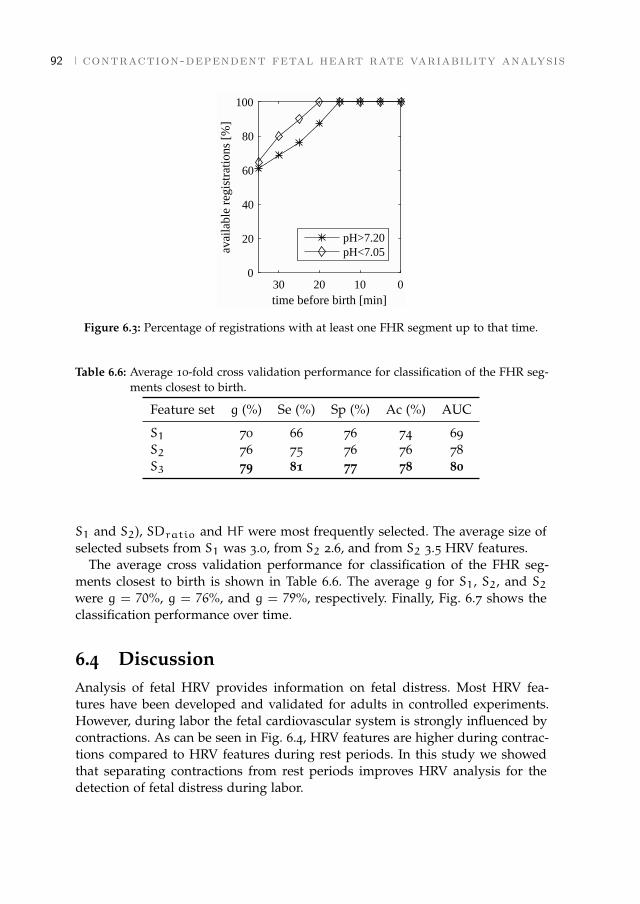
92 contraction-dependent fetal heart rate variability analysis
0102030time before birth [min]
0
20
40
60
80
100
avai
labl
e re
gist
ratio
ns [
%]
pH>7.20pH<7.05
Figure 6.3: Percentage of registrations with at least one FHR segment up to that time.
Table 6.6: Average 10-fold cross validation performance for classification of the FHR seg-ments closest to birth.
Feature set g (%) Se (%) Sp (%) Ac (%) AUC
S1 70 66 76 74 69S2 76 75 76 76 78S3 79 81 77 78 80
S1 and S2), SDratio and HF were most frequently selected. The average size ofselected subsets from S1 was 3.0, from S2 2.6, and from S2 3.5 HRV features.
The average cross validation performance for classification of the FHR seg-ments closest to birth is shown in Table 6.6. The average g for S1, S2, and S2were g = 70%, g = 76%, and g = 79%, respectively. Finally, Fig. 6.7 shows theclassification performance over time.
6.4 DiscussionAnalysis of fetal HRV provides information on fetal distress. Most HRV fea-tures have been developed and validated for adults in controlled experiments.However, during labor the fetal cardiovascular system is strongly influenced bycontractions. As can be seen in Fig. 6.4, HRV features are higher during contrac-tions compared to HRV features during rest periods. In this study we showedthat separating contractions from rest periods improves HRV analysis for thedetection of fetal distress during labor.
[ March 26, 2018 at 22:26 – classicthesis version 4.2 ]
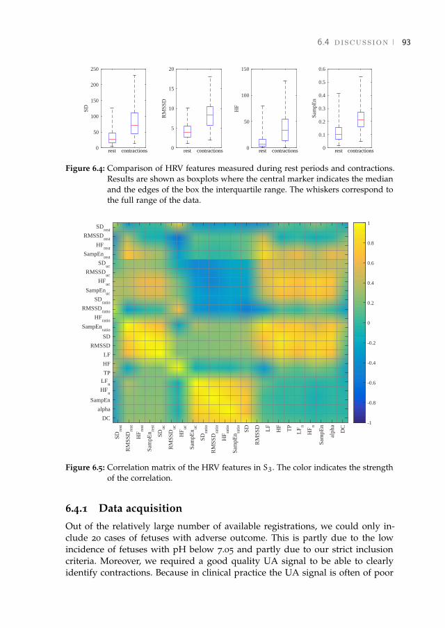
6.4 discussion 93
0
50
100
150
200
250
SD
rest contractions 0
5
10
15
20
RM
SSD
rest contractions 0
50
100
150
HF
rest contractions 0
0.1
0.2
0.3
0.4
0.5
0.6
Sam
pEn
rest contractions
Figure 6.4: Comparison of HRV features measured during rest periods and contractions.Results are shown as boxplots where the central marker indicates the medianand the edges of the box the interquartile range. The whiskers correspond tothe full range of the data.
SDre
st
RM
SSD
rest
HF
rest
Sam
pEn re
st
SDuc
RM
SSD
uc
HF
uc
Sam
pEn uc
SDra
tio
RM
SSD
ratio
HF
ratio
Sam
pEn ra
tio SD
RM
SSD LF
HF
TP
LF
n
HF
n
Sam
pEn
alph
a
DC
SDrest
RMSSDrest
HFrest
SampEnrest
SDuc
RMSSDuc
HFuc
SampEnuc
SDratio
RMSSDratio
HFratio
SampEnratio
SD
RMSSD
LF
HF
TPLF
nHF
n
SampEn
alpha
DC-1
-0.8
-0.6
-0.4
-0.2
0
0.2
0.4
0.6
0.8
1
Figure 6.5: Correlation matrix of the HRV features in S3. The color indicates the strengthof the correlation.
6.4.1 Data acquisition
Out of the relatively large number of available registrations, we could only in-clude 20 cases of fetuses with adverse outcome. This is partly due to the lowincidence of fetuses with pH below 7.05 and partly due to our strict inclusioncriteria. Moreover, we required a good quality UA signal to be able to clearlyidentify contractions. Because in clinical practice the UA signal is often of poor
[ March 26, 2018 at 22:26 – classicthesis version 4.2 ]
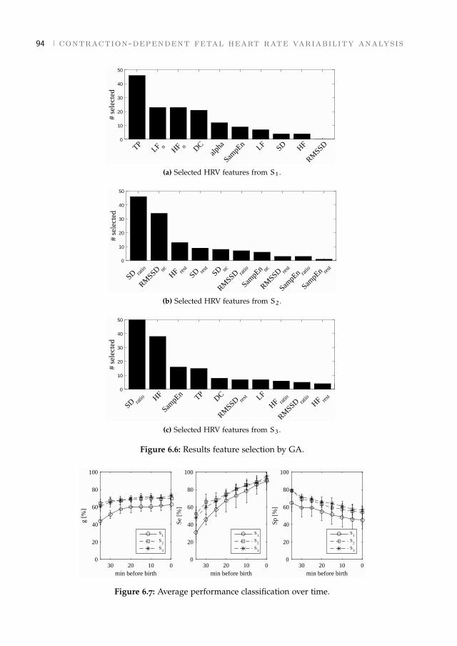
94 contraction-dependent fetal heart rate variability analysis
0
10
20
30
40
50
# se
lect
ed
TPLF n HF n DC
alpha
SampE
n LF SD HF
RMSSD
(a) Selected HRV features from S1.
0
10
20
30
40
50
# se
lect
ed
SD ratio
RMSSD uc
HF rest
SD rest
SD uc
RMSSD rat
io
SampE
n uc
RMSSD res
t
SampE
n ratio
SampE
n rest
(b) Selected HRV features from S2.
0
10
20
30
40
50
# se
lect
ed
SD ratio HF
SampE
n TPDC
RMSSD res
t LF
HF ratio
RMSSD rat
io
HF rest
(c) Selected HRV features from S3.
Figure 6.6: Results feature selection by GA.
0102030min before birth
0
20
40
60
80
100
g [%
]
S1
S2
S3
0102030min before birth
0
20
40
60
80
100
Se [
%]
S1
S2
S3
0102030min before birth
0
20
40
60
80
100
Sp [
%]
S1
S2
S3
Figure 6.7: Average performance classification over time.
[ March 26, 2018 at 22:26 – classicthesis version 4.2 ]

6.4 discussion 95
quality, this requirement limits the application of contraction-dependent HRVfeatures. A potential solution to improve the quality of the UA signal mightbe to use electrohysterography to record the UA instead of a tocodynamometer[176] and [115]. In addition to good quality UA signal, less than 20% loss of FHRsignal was allowed. To minimize the influence of artifact correction of the FHRsignal, periods with artifact corrected FHR were excluded from the calculationof HRV features.
In this study we only focussed on FHR segments during the second stage oflabor. During the second stage, contractions generally have a strong effect on thefetus. In contrast, during the first stage of labor (stage of cervical dilation), theeffect of contractions is less pronounced. Therefore, a classifier that is trained onFHR from the second stage of labor might be less predictive during the first stageof labor. For future work it would be interesting to also examine the classificationperformance during the first stage of labor.
Because the goal of this study was to examine whether separating contractionsfrom rest periods can improve the HRV analysis, we limited our dataset to twogroups that are well separated in terms of fetal outcome and did not considerregistrations with pH between 7.05 and 7.20. However, this approach simplifiesthe classification task and does not represent true clinical conditions. Before aclassifier can be used in clinical practice, future study should use a dataset thatcontains registration with all pH values.
6.4.2 Feature selection
Fig. 6.5 shows that several of the HRV features that were used in this studywere correlated. In particular, HRV features calculated on the entire FHR signalwere correlated to their counterpart that was calculated during contractions orduring rest periods (e.g. SD was correlated to SDrest and Suc). To select thebest combination of HRV features for detection of fetal distress we used GA. Theaverage size of selected subsets from S1, S2, and S3 (3.0, 2.6, and 3.5, respectively)was smaller than the maximum number of five features that was allowed for GA,indicating that larger feature subsets would not have improved classification.
Because GA uses the classification performance to score candidate subsets, se-lected HRV features could perform differently for other classifiers. Furthermore,since feature selection could be influenced by splitting the dataset in the 10-foldcross validation, GA was repeated fifty times using different data splits. The in-fluence of splitting the dataset on feature selection can be seen from Fig. 6.6 bythe number of HRV features that were selected multiple times.
The most frequently selected HRV feature for S1 was TP, and the most fre-quently selected HRV feature for S2 and S3 was SDratio. Although TP wasselected most of the time from S1, TP was only selected a few times for S3, asshown in Fig. 6.6. Since both TP and SDratio are related to the presence of decel-erations, these HRV features contain similar information. SDratio also containsinformation about how well the fetus is able to recover from contractions: a high
[ March 26, 2018 at 22:26 – classicthesis version 4.2 ]

96 contraction-dependent fetal heart rate variability analysis
SDratio indicates that the fetus quickly recovers from a contraction and is ableto stabilize its cardiovascular system during the rest periods. On the other hand,a low ratio indicates that the variability during contractions and rest periods issimilar, meaning that the fetus is unable to recover during the rest periods. Incase SDratio is selected, the information of TP becomes redundant.
Other HRV features that were often selected for S1 were LFn, HFn, and DC.In [31] it was also found that normalized spectral powers were predictive offetal distress. Since changes in normalized spectral powers are not masked bychanges in the total power, normalized spectral powers can give better insight incardiovascular control than absolute spectral powers.
Interestingly, although HFn was frequently selected for S1 it was not often se-lected for S3. Instead, for S3 HF was often selected in combination with SDratio.Since SDratio is related to the presence of decelerations and the total power, itcould be that the combination of SDratio and HF also contains the informationin HFn, since SDratio is related to TP. In line with the selection of HF for S3 isthe selection of RMSSDuc and HFrest for S2, as the combined information ofRMSSDuc and HFrest is similar to the information of HF.
To gain more insight in cardiovascular control, it would be interesting to ex-amine HFn and LFn during contractions and rest periods. However, the lengthof contractions or rest periods was often less than the required length to cal-culate LFn and HFn, and we were unable to calculate HFn and LFn separatelyduring contractions and rest periods. Besides LFn and HFn, in this study DCwas also frequently selected from S1, similar to findings in [179]. Since DC con-tains information about decelerations, it contains similar information as SDratioand was not frequently selected from S3. In our results, scaling exponent α wasselected less often. Recently, [165] obtained promising results for detection offetal distress by calculating scaling exponents using a wavelet based scatteringtransform. In [38] it was shown that the influence of decelerations on the scatter-ing transform is limited and using the scattering transform might improve thefractal analysis.
6.4.3 Classification
Many factors can influence the response of the fetus to contractions. There areclinical parameters that can influence the FHR, such as gestational age [190], be-havioral states [184], or medication [191]. Furthermore, uterine contractions candirectly influence the fetal cardiovascular system through a rise in intrauterinepressure, or indirectly by blocking the oxygen supply to the fetus (e.g. umbilicalcord occlusion) [192]. As labor progresses, the effect of contractions on the fetalcardiovascular system increases. As a consequence, in the literature many dif-ferent FHR patterns have been described with different characteristics, severalof which have been related to fetal distress (e.g. late decelerations, bradycardia,sinusoidal patterns, or saltatory patterns) [1]. The relatively low number of cases
[ March 26, 2018 at 22:26 – classicthesis version 4.2 ]
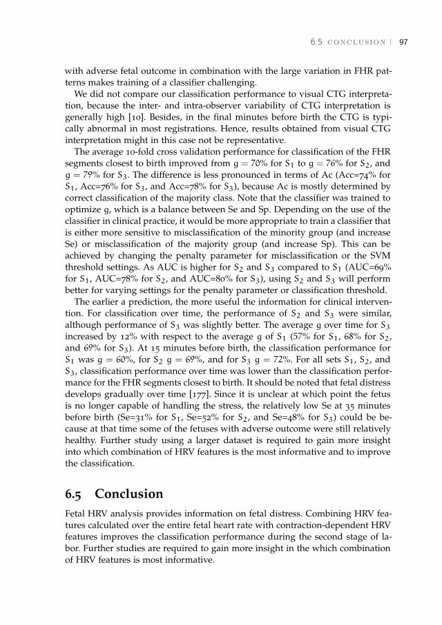
6.5 conclusion 97
with adverse fetal outcome in combination with the large variation in FHR pat-terns makes training of a classifier challenging.
We did not compare our classification performance to visual CTG interpreta-tion, because the inter- and intra-observer variability of CTG interpretation isgenerally high [10]. Besides, in the final minutes before birth the CTG is typi-cally abnormal in most registrations. Hence, results obtained from visual CTGinterpretation might in this case not be representative.
The average 10-fold cross validation performance for classification of the FHRsegments closest to birth improved from g = 70% for S1 to g = 76% for S2, andg = 79% for S3. The difference is less pronounced in terms of Ac (Acc=74% forS1, Acc=76% for S3, and Acc=78% for S3), because Ac is mostly determined bycorrect classification of the majority class. Note that the classifier was trained tooptimize g, which is a balance between Se and Sp. Depending on the use of theclassifier in clinical practice, it would be more appropriate to train a classifier thatis either more sensitive to misclassification of the minority group (and increaseSe) or misclassification of the majority group (and increase Sp). This can beachieved by changing the penalty parameter for misclassification or the SVMthreshold settings. As AUC is higher for S2 and S3 compared to S1 (AUC=69%for S1, AUC=78% for S2, and AUC=80% for S3), using S2 and S3 will performbetter for varying settings for the penalty parameter or classification threshold.
The earlier a prediction, the more useful the information for clinical interven-tion. For classification over time, the performance of S2 and S3 were similar,although performance of S3 was slightly better. The average g over time for S3increased by 12% with respect to the average g of S1 (57% for S1, 68% for S2,and 69% for S3). At 15 minutes before birth, the classification performance forS1 was g = 60%, for S2 g = 69%, and for S3 g = 72%. For all sets S1, S2, andS3, classification performance over time was lower than the classification perfor-mance for the FHR segments closest to birth. It should be noted that fetal distressdevelops gradually over time [177]. Since it is unclear at which point the fetusis no longer capable of handling the stress, the relatively low Se at 35 minutesbefore birth (Se=31% for S1, Se=52% for S2, and Se=48% for S3) could be be-cause at that time some of the fetuses with adverse outcome were still relativelyhealthy. Further study using a larger dataset is required to gain more insightinto which combination of HRV features is the most informative and to improvethe classification.
6.5 ConclusionFetal HRV analysis provides information on fetal distress. Combining HRV fea-tures calculated over the entire fetal heart rate with contraction-dependent HRVfeatures improves the classification performance during the second stage of la-bor. Further studies are required to gain more insight in the which combinationof HRV features is most informative.
[ March 26, 2018 at 22:26 – classicthesis version 4.2 ]

[ March 26, 2018 at 22:26 – classicthesis version 4.2 ]

7 F E TA L H E A RT R AT E VA R I A B I L I T Y D U R I N GP R E G N A N C Y
Abstract - Objective: Non-invasive spectral analysis of fetal heart rate variability isa promising new field of fetal monitoring. To validate this method properly, we studiedthe relationship between gestational age and the influence of fetal rest–activity state onspectral estimates of fetal heart rate variability. Design: Prospective longitudinal study.Setting: Tertiary care teaching hospital. Population: Forty healthy women with an un-eventful singleton pregnancy. Methods: Non-invasive fetal electrocardiogram measure-ments via the maternal abdomen were performed at regular intervals between 14 and40 weeks of gestation (wG) and processed to detect beat-to-beat fetal heart rate. Simul-taneous ultrasound recordings were performed to assess fetal rest–activity state. Mainoutcome measures. Absolute and normalized power of fetal heart rate variability in thelow (0.04–0.15 Hz) and high (0.4–1.5 Hz) frequency band were obtained, using FourierTransform. Results: 14% of all measurements and 3% of the total amount of abdominaldata (330 segments) was usable for spectral analysis. During 21–30 wG, a significantincrease in absolute low and high frequency power was observed. During the active statenear term, absolute and normalized low frequency power were significantly higher andnormalized high frequency power was significantly lower compared with the quiet state.Conclusions: The observed increase in absolute spectral estimates in preterm fetuses wasprobably due to increased sympathetic and parasympathetic modulation and might be asign of autonomic development. Further improvements in signal processing are neededbefore this new method of fetal monitoring can be introduced in clinical practice.1,2
1 Results in this chapter were obtained with signal processing methods that date back to 2012. Withthe methods presented in chapters 3 and 4, the percentage of recordings with usable fetal heartincreases from 14% to 66%.
2 This chapter is based on the paper published as Van Laar J.O.E.H., Warmerdam G.J.J., VerdurmenK.M.J., Vullings R., Peters C.H.L., Houterman S., Wijn P.F.F., Andriessen P., Van Pul C., Oei S.G., "Fetalheart rate variability in frequency-domain during pregnancy, obtained from noninvasive electrocardiogramrecordings". Acta Obstet Gynecol Scand. 2014, 93: 93-101.
[ March 26, 2018 at 22:26 – classicthesis version 4.2 ]
100 fetal hrv during pregnancy
7.1 IntroductionCardiotocography (CTG) is the widespread method for fetal monitoring, despiteits poor diagnostic value in detecting fetal distress [9]. The poor specificity of thismethod has resulted in increased rates of operative deliveries without a signifi-cant improvement in long-term fetal outcome [9]. Additional ST-waveform anal-ysis of the fetal electrocardiogram (ECG; STAN®, Neoventa Medical, Mölndal,Sweden) and fetal scalp blood sampling, applied in the case of a non-reassuringCTG, have a limited capability of improving neonatal outcome or reducing un-necessary interventions [9, 26, 27]. Besides, these techniques can only be usedduring labor at term due to their invasiveness. Therefore, there is an urgentneed to develop non-invasive methods that provide complementary informationon fetal well-being and that can be used intra- and antepartum during the termand preterm period.
The analysis of variations in beat-to-beat heart rate is an established non-invasive technique for investigating the autonomic cardiac control system [30]. Inhuman adults, heart rate variability (HRV) estimated by spectral analysis reflectsthe modulation of the sympathetic and parasympathetic limbs of the autonomicnervous system [30]. The low frequency cardiovascular fluctuations are ascribedto the baroreceptor reflex and are under sympathetic and parasympathetic con-trol, whereas high frequency fluctuations are associated with respiration and areunder parasympathetic control only [29, 30].
As in human adults, quantifying the variations in beat-to-beat fetal heart rate(FHR) by spectral analysis can be used to monitor autonomic nervous systemmodulation and may provide an early diagnostic tool for detection of fetal dis-tress [193]. Spectral analysis during labor was previously performed on beat-to-beat heart rate, obtained from direct fetal ECG recordings by scalp electrode [31,32, 184, 193]. Our previous studies during labor showed that spectral estimatesare associated with severe metabolic acidosis at birth [31] and might predict fetaldistress in an early stage [32]. In addition, spectral estimates are related to fetalbehavioral state and weeks of gestation (wG) during labor at term [184].
Before using spectral analysis for fetal monitoring, more insight needs to begained into normal autonomic development. However, at present, limited re-search has been done on human fetal HRV in the frequency-domain during thesecond and third trimester of pregnancy, and thus during the development ofautonomic reflex mechanisms [78, 79]. To measure spectral estimates during ges-tation, beat-to-beat FHR should be obtained non-invasively. Previous studies arelimited considering developmental aspects either because no longitudinal fol-low up was performed during pregnancy or because the studies did not takeinto account fetal movement during the third trimester. Changes in fetal HRVdue to fetal rest–activity state occur after 30 wG [85]. Since spectral estimatesof fetal HRV are known to be associated with rest–activity states at term gesta-tion [79, 184], it is difficult to interpret spectral values without classifying fetalmovements.
[ March 26, 2018 at 22:26 – classicthesis version 4.2 ]

7.2 material and methods 101
By measuring low frequency power (LF) and high frequency power (HF) atregular time intervals during gestation, the development of the fetal autonomiccardiac control can be examined. We developed a new method to obtain the fetalECG non-invasively from the maternal abdomen [45]. This method allows forbeat-to-beat detection of the fetal R-waves and provides fetal beat-to-beat heartrate and spectral estimates non-invasively.
The first objective of the current study is to present a non-invasive methodfor fetal ECG and beat-to-beat heart rate detection, and to evaluate its clinicalfeasibility. The second objective is to study the relationship between wG andspectral estimates of fetal HRV and to study the influence of fetal rest–activitystates on spectral estimates after 30 wG.
7.2 Material and methodsA prospective longitudinal study was performed in a tertiary care teaching hos-pital. The study protocol was approved by the institutional review board at theMáxima Medical Center (reference number 0650). Participants were recruitedconsecutively from a healthy population, undergoing routine pregnancy follow-up during one of the first outpatient visits. Only healthy women with an un-eventful singleton pregnancy, not taking medication other than iron tablets orvitamins, were asked to participate before 12 wG. Excluded were women underthe age of 18 years. Participants were included after a written informed consentform was signed. Pregnancy duration was determined from the last menstrualperiod and confirmed by crown–rump length at 10–12 wG. Only pregnancieswhich progressed uneventfully, resulting in the delivery of a healthy infant witha birth weight above the 10th percentile corrected for wG, maternal parity andfetal sex [194], were included in the data analysis.
7.2.1 Data acquisition and signal processing
Non-invasive fetal ECG measurements were repeatedly performed antenatally. Anon-invasive electrophysiological monitor for obstetrics (NEMO; Fig. 7.1a) wasused to record and store the data. The device has less than 5 µV root meansquare noise. The NEMO system was approved by the Medical Technical Ser-vice Department of the Máxima Medical Center. Recordings were performed atapproximately 14, 18, 22, 24, 26, 30, 34, 36, 38, and 40 wG. Measurements wereperformed non-invasively using eight self-adhesive electrodes, one reference andone ground electrode on the maternal abdomen (Fig. 7.1b). Each recording ses-sion took place between 8:00 h and 18:00 h, with the woman lying comfortablyin a bed in semi-recumbent position. During this time period, no importantfluctuations in fetal HRV were expected [195]. The duration of recordings wasapproximately 45 min. Simultaneous ultrasound recordings were performed toassess the fetal rest–activity state.
[ March 26, 2018 at 22:26 – classicthesis version 4.2 ]

102 fetal hrv during pregnancy
(a) (b)
Figure 7.1: (a) Prototype of the NEMO system. (b) Electrode configuration for antepartumfetal ECG recording. ECG, electrocardiography; GN, ground electrode; REF,reference electrode.
The abdominal data were analyzed off-line. The eight input signals wererecorded with a sample frequency of 1000 Hz. The signals were band-pass fil-tered between 1.5 and 70 Hz and a 50-Hz notch filter was used. The maternalECG waveform was estimated and subtracted from the signals. This was done bymeans of weighted averaging of maternal ECG segments [120]. Fig. 7.2a showsan example of a filtered abdominal signal of a 24-week pregnant woman, con-taining both maternal and fetal ECG. Fig. 7.2b shows the signal after subtractingthe maternal ECG. The eight resulting fetal ECG traces were processed to detectthe beat-to-beat FHR. The signal-to-noise ratio of these signals is enhanced byspatially combining the signals [196]. The fetal ECG in the combined signal isfurther enhanced by using the length transformation [197]. R-peaks are detectedin the transformed signal as peaks that exceed an adaptive threshold and thedetected R-peaks are then used to create the fetal beat-to-beat heart rate signals[196].
Spectral information about fetal beat-to-beat heart rate was obtained using aFourier Transform. Based on previous studies [106], as well as the physiologi-cal range of fetal heart and respiratory movement rate, the following frequencybands were chosen: total power (TP): 0.04– 1.5 Hz; LF: 0.04–0.15 Hz; HF: 0.4–1.5Hz. Beat-to-beat RR-intervals were re-sampled at 4 Hz to obtain equidistantlydistributed heart rates. To prevent aliasing, the Fourier Transform was calcu-lated in intervals of 64 s (based on 0.04 Hz, the lowest frequency of interest)[87]. The direct current component was subtracted before calculating the FourierTransform. To reduce spectral leakage, the signal was multiplied with a Parzenwindow function. After calculating the spectral power of fetal HRV, normalizedvalues were calculated by dividing LF and HF by TP (denoted as LFn and HFn,respectively).
[ March 26, 2018 at 22:26 – classicthesis version 4.2 ]
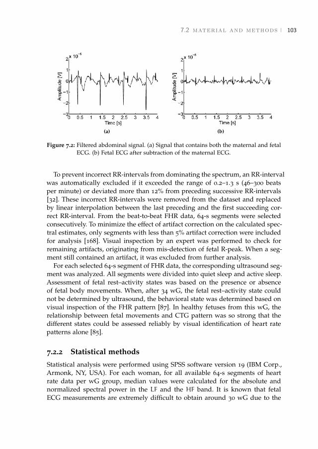
7.2 material and methods 103
(a) (b)
Figure 7.2: Filtered abdominal signal. (a) Signal that contains both the maternal and fetalECG. (b) Fetal ECG after subtraction of the maternal ECG.
To prevent incorrect RR-intervals from dominating the spectrum, an RR-intervalwas automatically excluded if it exceeded the range of 0.2–1.3 s (46–300 beatsper minute) or deviated more than 12% from preceding successive RR-intervals[32]. These incorrect RR-intervals were removed from the dataset and replacedby linear interpolation between the last preceding and the first succeeding cor-rect RR-interval. From the beat-to-beat FHR data, 64-s segments were selectedconsecutively. To minimize the effect of artifact correction on the calculated spec-tral estimates, only segments with less than 5% artifact correction were includedfor analysis [168]. Visual inspection by an expert was performed to check forremaining artifacts, originating from mis-detection of fetal R-peak. When a seg-ment still contained an artifact, it was excluded from further analysis.
For each selected 64-s segment of FHR data, the corresponding ultrasound seg-ment was analyzed. All segments were divided into quiet sleep and active sleep.Assessment of fetal rest–activity states was based on the presence or absenceof fetal body movements. When, after 34 wG, the fetal rest–activity state couldnot be determined by ultrasound, the behavioral state was determined based onvisual inspection of the FHR pattern [87]. In healthy fetuses from this wG, therelationship between fetal movements and CTG pattern was so strong that thedifferent states could be assessed reliably by visual identification of heart ratepatterns alone [85].
7.2.2 Statistical methods
Statistical analysis were performed using SPSS software version 19 (IBM Corp.,Armonk, NY, USA). For each woman, for all available 64-s segments of heartrate data per wG group, median values were calculated for the absolute andnormalized spectral power in the LF and the HF band. It is known that fetalECG measurements are extremely difficult to obtain around 30 wG due to the
[ March 26, 2018 at 22:26 – classicthesis version 4.2 ]

104 fetal hrv during pregnancy
presence of the vernix caseosa, which electrically shields the fetus from its sur-roundings [106]. Since changes in fetal HRV due to fetal rest–activity state onlyoccur after 30 wG [85], data were analyzed separately for the periods below andabove 30 wG. The median spectral estimates were plotted as a function of wG.Simple linear regression was used to study changes in spectral estimates overwG. For the group above 30 wG, analysis was repeated, restricted to fetal restand activity to examine the effect of fetal rest–activity state on the relationshipbetween spectral estimates and wG. In addition, for the group above 30 wG, themean values of the median spectral estimates were compared during the activeand quiet fetal state. An independent t-test was used to compare the active andquiet state. Statistical significance was assumed at an a-level of 0.05.
7.3 ResultsA total of 40 women were studied longitudinally during pregnancy. Measure-ments were performed from January 2007 to August 2009. From the 40 partic-ipants under study, three women were excluded because pregnancy was com-plicated by pregnancy-induced hypertension. In addition, two women were ex-cluded because of preterm labor. From the remaining data, 14% of all measure-ments contained one or more suitable data segments that could be used for spec-tral analysis. In total, 330, 64-s, segments of beat-to-beat heart rate data wereretrieved, accounting for 3% of the data. Fig. 7.3 shows the percentage of usablesegments for the different wG groups. The period until 21 wG was excludedfor further analysis, since only five 64-s segments of heart rate data could beretrieved. Furthermore, no segment could be retrieved in the period between30 and 34 wG. From the included 35 women, 10 were then excluded becausegood-quality fetal beat-to-beat heart rate could not be retrieved from the abdom-inal recordings. For the remaining 25 women included for analysis, a total of213 abdominal measurements were performed, from which 325 segments couldbe used for analysis. The mean number of measurements per woman was nine(standard deviation, SD, 1.6). The mean duration of each measurement was 42min (SD 9). All mothers delivered at term, and all neonates had a birth weightabove the 10th percentile. All neonates had an Apgar score of at least 8 at 1 minand at least 9 at 5 min. All neonates had an umbilical artery pH>7.05 and anumbilical artery base deficit 610. The characteristics of the women are given inTable 7.1.
Fig. 7.4 shows absolute LF and HF as a function of wG, for the period of21-30 and 34-41 wG. Fig. 7.5 shows LFn and HFn as a function of wG, for theperiod of 21–30 and 34–41 wG. From the available segments below 30 wG, fetalrest–activity state could be determined based on ultrasound recordings for 85segments (43%). Of these segments, 86% were retrieved during the active stateand 14% during the quiet state. In the group of 34-41 wG, rest–activity statecould be classified based on ultrasound recordings for 69 segments (54%). For
[ March 26, 2018 at 22:26 – classicthesis version 4.2 ]
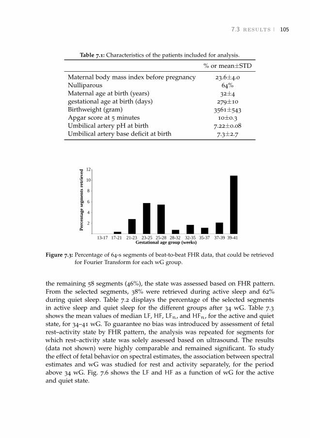
7.3 results 105
Table 7.1: Characteristics of the patients included for analysis.
% or mean±STD
Maternal body mass index before pregnancy 23.6±4.0Nulliparous 64%Maternal age at birth (years) 32±4gestational age at birth (days) 279±10Birthweight (gram) 3561±543Apgar score at 5 minutes 10±0.3Umbilical artery pH at birth 7.22±0.08Umbilical artery base deficit at birth 7.3±2.7
Gestational age group (weeks)13-17 17-21 21-23 23-25 25-28 28-32 32-35 35-37 37-39 39-41
Per
cen
tage
segm
ents
ret
riev
ed
12
10
8
6
4
2
Figure 7.3: Percentage of 64-s segments of beat-to-beat FHR data, that could be retrievedfor Fourier Transform for each wG group.
the remaining 58 segments (46%), the state was assessed based on FHR pattern.From the selected segments, 38% were retrieved during active sleep and 62%during quiet sleep. Table 7.2 displays the percentage of the selected segmentsin active sleep and quiet sleep for the different groups after 34 wG. Table 7.3shows the mean values of median LF, HF, LFn, and HFn, for the active and quietstate, for 34–41 wG. To guarantee no bias was introduced by assessment of fetalrest–activity state by FHR pattern, the analysis was repeated for segments forwhich rest–activity state was solely assessed based on ultrasound. The results(data not shown) were highly comparable and remained significant. To studythe effect of fetal behavior on spectral estimates, the association between spectralestimates and wG was studied for rest and activity separately, for the periodabove 34 wG. Fig. 7.6 shows the LF and HF as a function of wG for the activeand quiet state.
[ March 26, 2018 at 22:26 – classicthesis version 4.2 ]
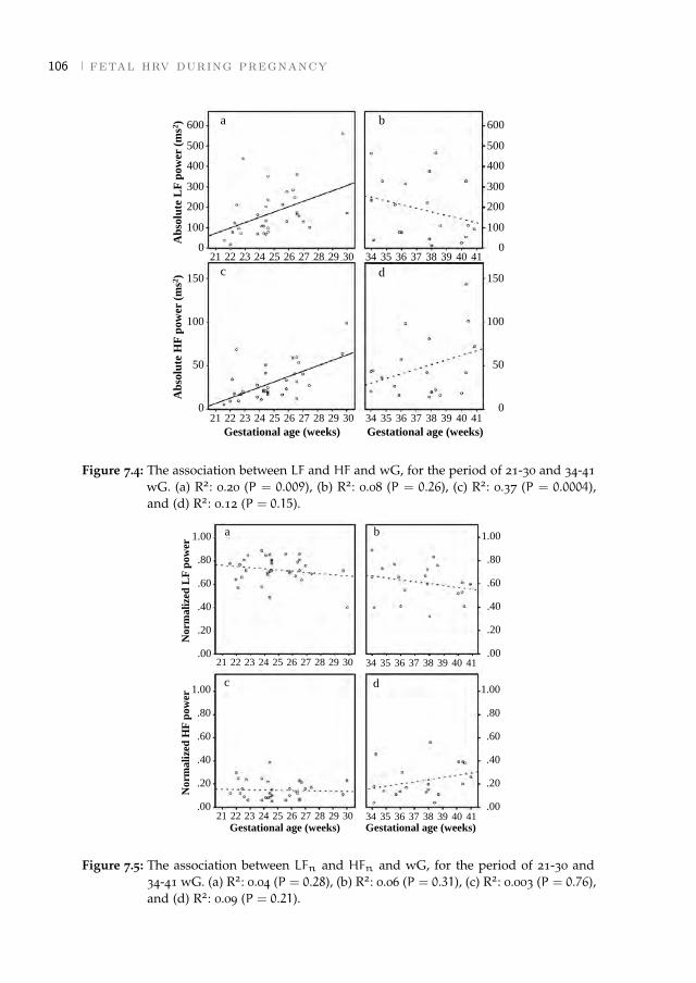
106 fetal hrv during pregnancy
150
100
50
0
Gestational age (weeks)
21 22 23 24 25 26 27 28 29 30 34 35 36 37 38 39 40 41
Gestational age (weeks)
21 22 23 24 25 26 27 28 29 30 34 35 36 37 38 39 40 41
ba
c d
Ab
solu
te L
F p
ow
er (
ms2
)A
bso
lute
HF
po
wer
(m
s2)
600
500
400
300
200
100
0
600
500
400
300
200
100
0
150
100
50
0
Figure 7.4: The association between LF and HF and wG, for the period of 21-30 and 34-41wG. (a) R2: 0.20 (P = 0.009), (b) R2: 0.08 (P = 0.26), (c) R2: 0.37 (P = 0.0004),and (d) R2: 0.12 (P = 0.15).
Gestational age (weeks)21 22 23 24 25 26 27 28 29 30 34 35 36 37 38 39 40 41
Gestational age (weeks)
21 22 23 24 25 26 27 28 29 30 34 35 36 37 38 39 40 41
ba
c d
Norm
ali
zed
LF
pow
erN
orm
ali
zed
HF
pow
er
1.00
.80
.60
.40
.20
.00
1.00
.80
.60
.40
.20
.00
1.00
.80
.60
.40
.20
.00
1.00
.80
.60
.40
.20
.00
Figure 7.5: The association between LFn and HFn and wG, for the period of 21-30 and34-41 wG. (a) R2: 0.04 (P = 0.28), (b) R2: 0.06 (P = 0.31), (c) R2: 0.003 (P = 0.76),and (d) R2: 0.09 (P = 0.21).
[ March 26, 2018 at 22:26 – classicthesis version 4.2 ]
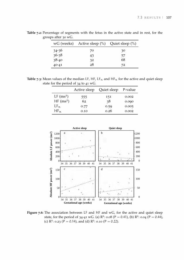
7.3 results 107
Table 7.2: Percentage of segments with the fetus in the active state and in rest, for thegroups after 30 wG.
wG (weeks) Active sleep (%) Quiet sleep (%)
34-36 70 3036-38 43 5738-40 32 6840-41 28 72
Table 7.3: Mean values of the median LF, HF, LFn and HFn for the active and quiet sleepstate for the period of 34 to 41 wG.
Active sleep Quiet sleep P-value
LF (ms2) 555 151 0.002HF (ms2) 62 38 0.090LFn 0.77 0.59 0.005HFn 0.10 0.26 0.002
Gestational age (weeks) Gestational age (weeks)
Ab
solu
te L
F p
ow
er (
ms2
)A
bso
lute
HF
po
wer
(ms2
)
150
100
50
034 35 36 37 38 39 40 4134 35 36 37 38 39 40 41
34 35 36 37 38 39 40 4134 35 36 37 38 39 40 41
150
100
50
0
1200
1000
800
600
400
200
0
1200
1000
800
600
400
200
0
Active sleep Quiet sleep
ba
c d
Figure 7.6: The association between LF and HF and wG, for the active and quiet sleepstate, for the period of 34-41 wG. (a) R2: 0.08 (P = 0.41), (b) R2: 0.04 (P = 0.44),(c) R2: 0.23 (P = 0.14), and (d) R2: 0.10 (P = 0.22).
[ March 26, 2018 at 22:26 – classicthesis version 4.2 ]
108 fetal hrv during pregnancy
7.4 DiscussionOur group developed a new method for non-invasive fetal ECG measurements[120, 196]. This new method can be used during periods in pregnancy, in whichother (invasive) techniques cannot be used for monitoring. Although Dopplerultrasound can also be used to obtain FHR non-invasively, ultrasound typicallyprovides a FHR that is averaged over a few cardiac cycles. This averaging affectsthe spectral information in the high frequency domain, virtually yielding onlyreliable information for the low frequency domain [33]. In addition, ultrasoundis sensitive to maternal and fetal movements and is therefore less suitable forprolonged measurements.
Our results in this study group showed that it is possible, although difficult, toretrieve fetal beat-to-beat heart rate from non-invasive abdominal fetal ECG mea-surements. Spectral analysis was feasible in 14% of all measurements; however,only 3% of the abdominal data was applicable for analysis. Due to the relativelylarge number of measurements without good-quality heart rate segments, wewere unable to statistically analyze the development of the spectral estimateson a case-based level. Thus, it is evident that further improvements in signalprocessing need to be made. The signal quality was independent of body massindex (BMI), since no significant difference (p = 0.9) was found between BMIof women included in our analysis (Table 7.1; 23.6, SD 4.0) and BMI of womenexcluded due to poor signal quality (23.3, SD 5.2). We were not able to retrievefetal beat-to-beat heart rate from the abdominal measurements before 18 andbetween 30 and 34 wG. Before 18 wG, this was probably due to the small size ofthe fetal heart. This results in a very low amplitude of the fetal ECG, renderingit undetectable on the maternal abdomen. Between 30 and 34 wG, the presenceof the vernix caseosa, which electrically isolates the fetal heart [106], probablycaused significant attenuation of the ECG signal. During the early preterm pe-riod (21–28 wG), approximately 5% of data was suitable for spectral analysis. Atterm, approximately 7% of data was suitable for spectral analysis. Probably, thedisappearance of the vernix caseosa and the relatively large fetal heart, madeit easier during the term period to detect the fetal signal from the combinedfetal–maternal signals measured on the maternal abdomen.
For the early preterm period, we observed a significant increase in LF andHF of fetal HRV with progressing pregnancy. We hypothesize that this increasewas due to increased sympathetic and parasympathetic modulation of the fetalheart, resulting from maturation of the fetal autonomic nervous system. This isin accordance with animal studies that showed an increase in sympathetic andparasympathetic cardiac modulation in premature fetuses, compared to imma-ture fetuses [83].
It is unlikely that the observed changes in spectral estimates before 30 wGwere due to changes in fetal breathing movements or rest–activity state. Al-though fetal breathing movements occurred as early as 10 wG [198], the HFpeak that was observed during breathing at term [199] could not be observed
[ March 26, 2018 at 22:26 – classicthesis version 4.2 ]

7.4 discussion 109
at 26 wG [200]. In addition, the incidence of fetal breathing movements did notchange between 24 and 28 wG [201]. The incidence of fetal movements decreasedas pregnancy progresses [202]. From 24 to 28 wG, a healthy fetus on averagemade 150–200 movements each hour [202]. Therefore, it was expected that mostselected 64-s segments of heart rate data below 30 wG were measured duringfetal activity, as was confirmed by our analysis of the corresponding ultrasoundmeasurements. In addition, LF was high in term fetuses during the active statecompared with quiescence [184]. Although short rest–activity cycles were firstnoticed at 23 wG, fetal HRV was similar during fetal activity and rest up to 30wG [85] and behavioral states could not be observed [203].
The observed increase in absolute LF and HF was not reflected in the normal-ized values during the early preterm period. This might be due to a comparablerelative increase in both LF and HF.
For the (near) term fetuses, a non-significant decrease in LF and a non-significantincrease in HF were observed. A decrease in LF after 30 wG was also describedby David et al. [79]. Fetal activity is known to increase fetal HRV from approx-imately 30 wG onwards [85], and a decrease in fetal movements with wG wasreported [202]. Therefore, a LF decrease after 30 wG is expected to occur due toa decrease in fetal movements. Later in pregnancy, starting in the 34th week ofgestation, fetal behavioral states appear [86]. As these states are partly definedon the basis of HRV, it seems relevant to consider them in the interpretation ofHRV measures.
Furthermore, LF and LFn were found to be significantly higher and HFn sig-nificantly lower during fetal activity compared with at rest. A non-significantincrease in HF was observed during the active state. These results were similarto those obtained with invasive measurements during labor at term [184].
If analysis was repeated with restriction to periods of fetal rest and activity (asshown in Fig. 7.6), LF increased non-significantly as a function of wG during ac-tivity, whereas LF decreased non-significantly during rest. Since for the selectedsegments the time spent in rest increased with wG during the (near) term pe-riod (as shown in Table 7.2), a decrease in fetal activity might explain the overalldecrease in LF as pregnancy progresses.
In post term fetuses, an increase in both HF and HFn was found in our pre-vious studies with invasive measurements, in relation to the near term group[184]. We observed a similar trend towards increased HF and HFn near term inthe present study. Because this trend was independent of fetal rest–activity state,it cannot be explained by changes in fetal behavior. This trend might suggestcontinuing parasympathetic maturation during the term period and increasinginfluence of the vagal system. This is in line with Assali et al. [83] who founda marked rise in parasympathetic tone during the neonatal period, up until theadult state.
[ March 26, 2018 at 22:26 – classicthesis version 4.2 ]

110 fetal hrv during pregnancy
7.5 ConclusionsOur non-invasive fetal ECG method enables us to measure fetal HRV in frequency-domain during the early preterm and term period. Our results are in accordancewith those seen in animal studies and with the previous literature regarding in-vasive measurements during labor. This is the first study that measures spectralestimates longitudinally and relates spectral estimates to fetal behavioral state.Further progress in signal processing will enable improved study of the relation-ship between spectral estimates and wG, allowing for longitudinal analysis.
[ March 26, 2018 at 22:26 – classicthesis version 4.2 ]
8 T H E I N F L U E N C E O F B E TA M E T H A S O N E O N F E TA LH E A RT R AT E VA R I A B I L I T Y
Abstract - Background: Betamethasone is widely used to enhance fetal lung matura-tion in case of threatened preterm labor. Fetal heart rate variability is one of the mostimportant parameters to assess in fetal monitoring, since it is a reliable indicator forfetal distress. Aim: To describe the effect of betamethasone on fetal heart rate variability,by applying spectral analysis on non-invasive fetal electrocardiogram recordings. Studydesign: Prospective cohort study. Subjects: Patients that require betamethasone, with agestational age from 24 weeks onwards.Outcome measures: Fetal heart rate variabil-ity parameters on day 1, 2, and 3 after betamethasone administration are compared toa reference measurement. Results: Following 68 inclusions, 12 patients remained withcomplete series of measurements and sufficient data quality. During day 1, an increasein absolute fetal heart rate variability values was seen. During day 2, a decrease inthese values was seen. All trends indicate a return to pre-medication values on day 3.Normalised high- and low-frequency power show little changes during the study pe-riod. Conclusions: The changes in fetal heart rate variability following betamethasoneadministration show the same pattern when calculated by spectral analysis of the fetalelectrocardiogram, as when calculated by cardiotocography. Since normalised spectralvalues show little changes, the influence of autonomic modulation is minor.1,2
1 Results in this chapter were obtained with signal processing methods that date back to 2012. Withthe methods presented in chapters 3 and 4, the percentage of recordings with usable fetal heartincreases from 60% to 86%.
2 This chapter has been accepted for publication as Verdurmen K.M., Warmerdam G.J.J., Lempersz C.,Hulsenboom O., Renckens J., Dieleman J., Vullings R., Van Laar J.O.E.H., Oei S.G., "The influence ofbetamethasone on fetal heart rate variability, obtained by noninvasive fetal electrocardiogram recordings".
[ March 26, 2018 at 22:26 – classicthesis version 4.2 ]
112 betamethasone and fetal heart rate variability
8.1 IntroductionCardiotocography (CTG) is used for fetal monitoring worldwide. One of themost important parameters to assess in CTG monitoring is fetal heart rate vari-ability (HRV). Normal fetal HRV is a reliable indicator of fetal wellbeing, whiledecreased fetal HRV is associated with poor neonatal outcome (acidosis, lowApgar score and death) [204]. The fetal heart rate (FHR), and thus HRV, is regu-lated by a complex interplay of the sympathetic and parasympathetic branchesof the autonomic nervous system [66]. Spectral analysis of fetal HRV can beused to quantify these changes in autonomic regulation [31, 32, 184, 193, 205].Low frequency power (LF) reflects baroreceptor reflex activity, and is both sym-pathetically and parasympathetically mediated [30]. High frequency power (HF)is associated with fetal respiration, and is solely parasympathetically mediated[30].
Antenatal betamethasone administration plays an important role in the clin-ical management of threatened preterm delivery between 24 and 34 weeks ofgestation (wG). It enhances fetal lung maturation and results in a significantreduction in, amongst others, neonatal mortality and respiratory distress syn-drome [206]. However, betamethasone can easily cross the placenta [207] andinfluence fetal autonomic modulation and thus fetal HRV. Since fetal HRV is animportant marker for fetal distress, knowledge on the influence of betametha-sone on autonomic regulation is needed to avoid misinterpretation of changesin fetal HRV following betamethasone administration, and therefore prevent un-necessary iatrogenic preterm delivery.
Results of previous studies describing the effect of betamethasone on fetalHRV indicate that fetal HRV increases during the first day, followed by a de-crease during days 2-3 [191]. Values returned to baseline during day 4. However,these studies were performed using CTG and measured the FHR by Doppler-ultrasound. With CTG, the FHR is averaged over several heartbeats and there-fore beat-to-beat information is lacking. As a consequence, it is not possible toperform reliable spectral analysis.
The aim of this study is to quantify the effects of maternally administeredbetamethasone on spectral values of fetal HRV. To perform a reliable calcula-tion of LF and HF we extracted beat-to-beat FHR information from non-invasiveabdominal fetal ECG recordings [208].
8.2 Materials and MethodsWe performed a prospective, longitudinal cohort study at the Máxima MedicalCenter, Veldhoven, the Netherlands. This is a tertiary care teaching hospital forobstetrics. The study protocol was approved by the Medical Ethical Committeeof the Máxima Medical Center. Participants were included after written informedconsent.
[ March 26, 2018 at 22:26 – classicthesis version 4.2 ]
8.2 materials and methods 113
8.2.1 Study population
As described in our study protocol, we aimed for at least 50 inclusions andexpected to end with 10-20 complete sets of measurements due to the antic-ipated loss to follow-up in this study group. We were not able to perform apower calculation, since this is the first study describing a five-day follow-upperiod following betamethasone administration with non-invasive abdominalfetal ECG recordings. From March 2013 until July 2016, women with a singletonpregnancy, at risk for preterm delivery and admitted to the Obstetric High Careunit were asked to participate in this study. All women requiring betametha-sone (Celestone Chrondose®, Schering AG, Berlin, Germany; 2 doses of 12mgintramuscularly, 24 hours apart) as part of standard clinical management wereeligible to participate. In case of threatened preterm labor, co-administration oftocolytic drugs was allowed. Nifedipine was used to attenuate uterine contrac-tions, occasionally complemented by indomethacin in case of continuous uterinecontractions when betamethasone administration was not yet completed. In caseof preterm prelabor rupture of membranes, patients also received antibiotics(erythromycin 250mg 4 times daily during 10 days) as part of the standard treat-ment protocol. Women were excluded in case of maternal age <18 years, multiplepregnancy, fetuses with a known congenital malformation, signs of intra-uterineinfection or fetal growth restriction (defined as the estimated weight of the fetusbelow the 5th percentile for gestational age).
The following data were gathered prospectively: maternal gravidity and parity,indication for betamethasone administration, obstetrical and general medical his-tory, gestational age at inclusion and administered medication during the studyperiod. Follow-up measurements of study participants lasted from the date of in-formed consent until five days after the first measurement, discharge or delivery,whichever occurred first. Postpartum, neonatal charts were checked for any in-dications of congenital anomalies that might have influenced the measurementsand for missed cases of growth restriction defined as birth weight below the 5thpercentile (corrected for gestational age, parity and sex of the neonate).
8.2.2 Measurements
We performed series of measurements as visualised in Fig. 8.1. Recordings wereobtained while the patient was lying in a semi-recumbent position, to preventsupine hypotension syndrome. To reduce the influence of diurnal variations, thetiming of measurements within a series was fixed for each patient (between 20and 28 hours after the previous measurement). In order to respect the patient’snight rest, no measurements were performed between 24.00h and 7.00h.
Most patients were transferred from secondary care hospitals in the region.Since for these patients betamethasone treatment was initiated prior to transport,they had no baseline measurement (0-measurement, on day 0). Former researchshowed that all changes in FHR and fetal HRV returned to baseline values from
[ March 26, 2018 at 22:26 – classicthesis version 4.2 ]
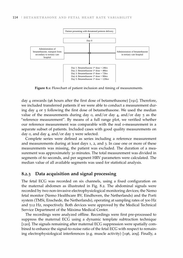
114 betamethasone and fetal heart rate variability
Patient presenting with threatened preterm delivery
Day 0
Administration of
betamethasone, transport from
secondary to tertiary care
hospital
Day 1: Betamethasone 1st dose + 24hrs
Day 2: Betamethasone 1st dose + 48hrs
Day 3: Betamethasone 1st dose + 72hrs
Day 4: Betamethasone 1st dose + 96hrs
Day 5: Betamethasone 1st dose + 120hrs
Administration of betamethasone
in tertiary care hospital
Figure 8.1: Flowchart of patient inclusion and timing of measurements.
day 4 onwards (96 hours after the first dose of betamethasone) [191]. Therefore,we included transferred patients if we were able to conduct a measurement dur-ing day 4 or 5 following the first dose of betamethasone. We used the medianvalue of the measurements during day 0, and/or day 4, and/or day 5 as the“reference measurement”. By means of a full range plot, we verified whetherour reference measurement was comparable with the real 0-measurement in aseparate subset of patients. Included cases with good quality measurements onday 0, and day 4, and/or day 5 were selected.
Complete series were defined as series including a reference measurementand measurements during at least days 1, 2, and 3. In case one or more of thesemeasurements was missing, the patient was excluded. The duration of a mea-surement was approximately 30 minutes. The total measurement was divided insegments of 60 seconds, and per segment HRV parameters were calculated. Themedian value of all available segments was used for statistical analysis.
8.2.3 Data acquisition and signal processing
The fetal ECG was recorded on six channels, using a fixed configuration onthe maternal abdomen as illustrated in Fig. 8.2. The abdominal signals wererecorded by two non-invasive electrophysiological monitoring devices; the Nemofetal monitor (Nemo Healthcare BV, Eindhoven, the Netherlands) and the Portisystem (TMSi, Enschede, the Netherlands), operating at sampling rates of 500 Hzand 512 Hz, respectively. Both devices were approved by the Medical TechnicalService Department of the Máxima Medical Center.
The recordings were analyzed offline. Recordings were first pre-processed tosuppress the maternal ECG using a dynamic template subtraction technique[120]. The signals remaining after maternal ECG suppression were spatially com-bined to enhance the signal-to-noise ratio of the fetal ECG with respect to remain-ing electrophysiological interferences (e.g. muscle activity) [196, 209]. Finally, a
[ March 26, 2018 at 22:26 – classicthesis version 4.2 ]

8.2 materials and methods 115
Figure 8.2: The six channel fetal electrocardiogram is recorded with electrodes on thematernal abdomen, placed in a fixed configuration. The ground (GND) andreference (REF) electrode are placed near the belly button. The electrodes areconnected to a battery operated data acquisition system (Nemo HealthcareBV), which filters, amplifies, and digitises the data for further processing. Thissystem is connected to a computer.
wavelet-based R-peak detection was performed to obtain a beat-to-beat FHR[150]. In case no R-peaks were detected using all six channels, channels withgood quality fetal ECG were selected manually to avoid negative effects on thespatial combination of those channels that were dominated by interferences.
Prior to HRV analysis, the obtained heart rates were automatically analyzedfor incorrect RR-intervals. RR-intervals shorter than 0.3 seconds or longer than1.2 seconds (<50 or >200 bpm) were assumed to be incorrect [150]. Furthermore,if an RR-interval deviated more than 12% from a running average RR-interval, itwas also assumed to be incorrect [168]. The incorrect RR-intervals were replacedby linear interpolation. To ensure reliable spectral analysis, only heart rate seg-ments of 60 seconds were included with less than 20% interpolation and lessthan five seconds of consecutive interpolation [168]. We only included measure-ments with at least three segments that met the quality criteria.
8.2.4 Heart rate variability analysis
Fetal HRV was quantified using both time-domain features (short-term variabil-ity, STV , and long-term variability, LTV) and features from spectral analysis (LFand HF). The obtained heart rates were resampled at 4 Hz by linear interpolation,since spectral analysis requires equidistantly distributed signals.
Spectral analysis was performed using a continuous wavelet transform [166].Based on previous studies, the following frequency bands were selected: 0.04-1.5Hz for the total power (TP), 0.04-0.15 Hz for LF, and 0.4-1.5 Hz for HF [30, 32,184, 210, 211]. LF and HF were expressed in absolute units (ms2) and normalisedunits (LFn = LF/TP, HFn = HF/TP).
[ March 26, 2018 at 22:26 – classicthesis version 4.2 ]

116 betamethasone and fetal heart rate variability
In addition to spectral powers, STV and LTV were calculated to compare ourresults to prior research performed with CTG measurements. LTV was calcu-lated as the difference between the maximum and minimum RR-interval in ev-ery 60 seconds segment [34, 212]. STV was calculated as the mean of absolutedifferences between consecutive RR-intervals in every 60 seconds segment [34].Note that in CTG (ultrasound) monitoring, STV is defined based on epochs (e.g.1/16th of a minute) because FHR is not acquired beat-to-beat. However, sincethe gold standard for STV is beat-to-beat variation [212], we used the aforemen-tioned ECG-based STV calculation.
8.2.5 Statistical analysis
Descriptive statistics were used to describe the study population and outcomemeasures. No further statistical analysis was performed. For each fetus a differ-ent number of segments were available during the study period, mainly due tovariations in ECG signal quality. The result on each day was compared to thereference measurement.
8.3 ResultsThe inclusion process is depicted in Fig. 8.3. Initially, 68 women were includedin this study. Three patients requested withdrawal from the study because ofpoor prognosis for an extreme premature child (1), technical issues (1) and in-convenient timing of measurements for the patient (1). In one patient unexpectedintra-uterine fetal death occurred during the study period. Extensive evaluationrevealed no evident cause. In 28 patients we were able to obtain a complete setof measurements, of which 16 were excluded due to insufficient data quality(less than three good quality segments per measurement) in one or more of themeasurements. Eventually, 12 patients were included with a complete set of suf-ficient data quality. Table 8.2 shows the patient characteristics of the includedcases. The amount of available segments for analysis is displayed in Table 8.1.
Measurements during day 0, and/or day 4, and/or day 5 were compared infive patients. In Fig. 8.4, LF, HF, LFn, and HFn are displayed. As expected, theabsolute fetal HRV values showed some inter- and intra-patient variation, whichcan mainly be explained by variation in the segments that were recorded duringactive and quiet states and by variation in gestational age of the fetuses. LFn andHFn show better comparability during day 0, 4, and 5, since these normalisedvalues are not masked by changes in total power. For instance, these values arenot influenced by fetal activity states.
Our outcome of interest was fetal HRV. Descriptively, in Fig. 8.5 we see anincrease in LTV and STV on day 1, and a decrease on day 2 and 3 as comparedto the reference measurement. For LF and HF, we see the same trend. For LFnand HFn we see little changes during the study period.
[ March 26, 2018 at 22:26 – classicthesis version 4.2 ]

8.3 results 117
68 inclusions
Exclusions: 19- Congenital anomaly 4
- Cardiac arrhythmia 1
- Fetal growth restriction 1
- No betamethasone administration 6
- Measurements* 7
Drop-out: 21- Preterm labour 10
- Discharged 7
- Withdrawal 3
- Stillbirth 1
28 complete series
of measurements16 series with insufficient data quality
12 series with sufficient data quality
*Patients were excluded if the measurements were not performed within the time window (between20 and 28 hours after the previous measurement), had one or more missing measurement in theseries, or were insufficient in data quality.
Figure 8.3: Overview of the inclusion process.
Table 8.1: Amount of segments available for analysis.
Segments for analysis/ Percentage oftotal segments segments for analysis
Reference measurementDay 0a 103/110 94%Day 4 201/305 66%Day 5b 162/278 58%
Day 1 332/580 57%Day 2 214/403 53%Day 3 223/407 55%
a Day 0: measurements performed in 3 out of 12 patients.b Day 5: measurements performed in 9 out of 12 patients.On the other study days, measurements were performed in all 12 patients.
[ March 26, 2018 at 22:26 – classicthesis version 4.2 ]

118beta
meth
aso
ne
an
dfeta
lh
eart
rate
var
iability
Table 8.2: Patient characteristics and pregnancy outcome.
case Maternal Indication Relevant history wG at Medication wG at Birth weight Apgar NICUgravidity, inclusion (not betamethasone) delivery percentilea score admissionparity 1/5´
1 G1P0 TPL - 24+4 Nifedipine,indomethacin, 25+4 50 7/8 YesLMWH
2 G1P0 PE May-Turner, 33+4 LMWH,methyldopa 34+3 5-10 9/10 Nothrombosis,
3 G2P1 VBL Gestational diabetes 31+1 Progesterone (vaginal), 33+5 50-80 9/10 Nonifedipine, augmentin
4 G2P1 PPROM - 33+0 Nifedipine, erythromycin 34+1 50-80 8/9 No5 G2P1 TPL - 26+2 Nifedipine, 39+5 50-80 5/9 No6 G1P0 TPL LEEP 29+2 Nifedipine, 40+1 80 9/10 No7 G1P0 VBL - 25+2 - 38+1 20-50 9/10 No8 G2P1 TPL Pre-existent 26+1 Nifedipine,labetalol, 36+6 50-80 8/10 No
hypertension magnesium sulphate,indomethacin
9 G2P1 TPL - 25+6 Nifedipine, progesterone 40+4 50 9/10 No(vaginal)
10 G2P1 VBL - 33+0 Iron tablets 37+5 90-95 9/10 No11 G1P0 TPL - 30+6 Nifedipine 32+6 >97 9/10 No12 G1P0 VBL LEEP 26+6 - 33+5 50-80 ?/10 No
a Birth weight percentile: percentiles are corrected for parity, gestational age at delivery and sex, and apply to the Dutch population.Source: Perined.Abbreviations: LEEP = loop electrosurgical excision procedure of the cervix, LMWH = low molecular weight heparin, NICU = neonatalintensive care unit, PE = pre-eclampsia, PPROM = premature prelabor rupture of membranes, TPL = threatened preterm labor, VBL= vaginal blood loss.
[March
26,2018at
22:26–classicthesis
version4.2
]
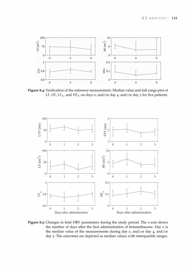
8.3 results 119
0 4 50
75
150L
F (m
s2 )
0 4 50
6
12
HF
(ms2 )
0 4 50.6
0.8
1
LFn
0 4 50
0.1
0.2
HFn
Figure 8.4: Verification of the reference measurement. Median value and full range plot ofLF, HF, LFn, and HFn on days 0, and/or day 4, and/or day 5 for five patients.
0 1 2 30
50
100
LT
V (
ms)
0 1 2 31
2
3
STV
(m
s)
0 1 2 30
50
100
LF
(ms2 )
0 1 2 30
5
10
HF
(ms2 )
0 1 2 3Days after administration
0.6
0.8
1
LF
n
0 1 2 3Days after administration
0
0.1
0.2
HF
n
Figure 8.5: Changes in fetal HRV parameters during the study period. The x-axis showsthe number of days after the first administration of betamethasone. Day 0 isthe median value of the measurements during day 0, and/or day 4, and/orday 5. The outcomes are depicted as median values with interquartile ranges.
[ March 26, 2018 at 22:26 – classicthesis version 4.2 ]
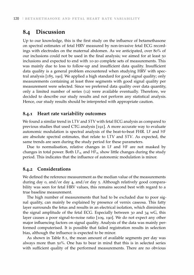
120 betamethasone and fetal heart rate variability
8.4 DiscussionUp to our knowledge, this is the first study on the influence of betamethasoneon spectral estimates of fetal HRV measured by non-invasive fetal ECG record-ings with electrodes on the maternal abdomen. As we anticipated, over 80% ofour inclusions could not be used in the final analysis; we aimed for at least 50inclusions and expected to end with 10-20 complete sets of measurements. Thiswas mainly due to loss to follow-up and insufficient data quality. Insufficientdata quality is a general problem encountered when studying HRV with spec-tral analysis [185, 190]. We applied a high standard for good signal quality; onlymeasurements containing at least three segments with good signal quality permeasurement were selected. Since we preferred data quality over data quantity,only a limited number of series (12) were available eventually. Therefore, wedecided to describe our study results and not perform any statistical analysis.Hence, our study results should be interpreted with appropriate caution.
8.4.1 Heart rate variability outcomes
We found a similar trend in LTV and STV with fetal ECG analysis as compared toprevious studies that used CTG analysis [191]. A more accurate way to evaluateautonomic modulation is spectral analysis of the beat-to-beat FHR. LF and HFare absolute spectral estimates, that relate to LTV and STV . As expected, thesame trends are seen during the study period for these parameters.
Due to normalisation, relative changes in LF and HF are not masked bychanges in total power. Both LFn and HFn show little changes during the studyperiod. This indicates that the influence of autonomic modulation is minor.
8.4.2 Considerations
We defined the reference measurement as the median value of the measurementsduring day 0, and/or day 4, and/or day 5. Although relatively good compara-bility was seen for fetal HRV values, this remains second best with regard to atrue baseline measurement.
The high number of measurements that had to be excluded due to poor sig-nal quality, can mainly be explained by presence of vernix caseosa. This fattylayer surrounds the fetus and results in an electrical isolation, which diminishesthe signal amplitude of the fetal ECG. Especially between 30 and 34 wG, thislayer causes a poor signal-to-noise ratio [109, 190]. We do not expect any othermajor influencing factors on signal quality. Analysis of the data was mainly per-formed computerised. It is possible that failed registration results in selectionbias, although the influence is expected to be minor.
As shown in Table 8.1, the mean amount of available segments per day wasalways more than 50%. One has to bear in mind that this is in selected serieswith sufficient quality of the performed measurements. There are no obvious
[ March 26, 2018 at 22:26 – classicthesis version 4.2 ]
8.4 discussion 121
differences between the measurement days; the amount of available segments issteady between 52% and 57%. Only the measurements performed on day 0 showa higher percentage of available segments. However, only 3 out of 12 patientswere eligible for a measurement during day 0.
By including patients receiving other pregnancy-related drugs rather than be-tamethasone, we aimed to obtain information that is applicable in daily clinicalpractice. Nifedipine and indomethacin seem to have no clinically important ef-fect on fetal HRV, while magnesium sulphate can cause decreased fetal HRV andcases of bradycardia have been described [104]. In one case, magnesium sulphatewas administered during days 1, 2 and 3 of the study period. Since magnesiumsulphate was not administered during the reference measurement, this mighthave had some influence on the study results. In one case labetalol was adminis-tered to the patient; this was already started prior to the measurements and nochanges in dosage occurred during the study period. Therefore, it is not likelythat this had major influence on the study results. It is unlikely for amoxicillin-clavulanic acid, low-molecular weight heparin, methyldopa and progesterone tohave any influence on fetal HRV parameters due to their mechanism of action.
Apart from pathological conditions, two major factors that one should con-sider when assessing FHR patterns are gestational age and fetal behaviouralstates [97]. Previous studies show that gestational age significantly affects the fe-tal HRV power spectrum, with a gradual increase in LF and HF during gestation[77, 79, 190]. In this study, the included fetuses had a gestational age varyingfrom 24 to 33 wG. Since we studied fetuses on successive days and were inter-ested in relative changes in fetal HRV parameters, the influence of the increasein LF and HF during gestation is likely to be minor. This study demonstrated anincrease in time spent in the quiet state following betamethasone administration.This might be caused by disturbance of the maternal glucose metabolism [213],which is a known side effect of corticosteroids.
Fetal HRV and fetal movements are two parameters associated with fetal well-being. The reduction in both, due to betamethasone administration, can be mis-interpreted as fetal deterioration and can therefore possibly lead to unnecessaryiatrogenic preterm delivery [214, 215]. Most likely, the reduction in fetal move-ments is a direct effect of corticosteroid administration, possibly by occupyingthe glucocorticosteroid receptor in the central nervous system, suppressing neu-ronal activity and therefore reducing physical activity in the fetus [191]. Noother signs of fetal hypoxia, like decelerations or abnormalities in Doppler flowvelocity waveforms, have occurred after corticosteroid administration [214–218].In addition, Shenhav et al. [219] demonstrated that reduced fetal HRV was notrelated to the fetal acid-base balance at birth when delivery occurred <48 hoursfollowing betamethasone administration. This study confirms these results, sincethe influence of autonomic modulation was found to be minor (reflected as noevident changes in normalised spectral powers during the study period). How-ever, in fetal monitoring it is important to be aware of the side-effects, such asreduced fetal HRV and fetal movements.
[ March 26, 2018 at 22:26 – classicthesis version 4.2 ]

122 betamethasone and fetal heart rate variability
8.5 ConclusionThe changes in fetal HRV following betamethasone administration show thesame pattern when calculated by spectral analysis of the fetal ECG, as whencalculated by Doppler-ultrasound CTG. Since normalised spectral values showlittle changes, the influence of autonomic modulation is minor.
[ March 26, 2018 at 22:26 – classicthesis version 4.2 ]
9 D I S C U S S I O N A N D F U T U R E D I R E C T I O N S
9.1 DiscussionMonitoring of the fetal condition and early recognition of fetal distress are ofvital importance to ensure timely intervention. One of the most important fea-tures to assess in fetal monitoring is fetal heart rate variability (HRV) [7]. Sincethe autonomic nervous system (ANS) controls the fetal heart rate (FHR), changesin fetal HRV are indicative of ANS regulation and can indirectly provide infor-mation about fetal distress [29, 30]. Recent studies have shown interest in com-puterized analysis of fetal HRV for detection of fetal distress [31–39]. However,most clinicians currently use Doppler ultrasound (US) to monitor the FHR. SinceFHR from Doppler US can only provide an averaged FHR, its use for computer-ized analysis of fetal HRV is limited. Instead of the averaged FHR from DopplerUS, a beat-to-beat FHR can be obtained from the fetal electrocardiogram (ECG).Besides accurate FHR information, the fetal ECG also provides additional mor-phology information that could be used to assess the fetal condition [13, 15, 19,47]. Unfortunately, in clinical practice the fetal ECG is currently only availablevia invasive measurement using a scalp electrode. Hence, the fetal ECG can onlybe obtained during labor after sufficient cervical dilation and after the fetal mem-branes have ruptured.
The fetal ECG can also be recorded non-invasively with electrodes on thematernal abdomen. However, the non-invasiveness comes at the expense of typ-ically low signal to noise ratios (SNR) of the fetal ECG. In the first part of thisthesis we focused on improving signal quality and reliability of FHR detection.In addition to these technical challenges, it is also necessary to study the physi-ological context in which the acquired FHR can be used for computerized HRVanalysis. In the second part of this thesis we focused on the application of com-puterized analysis of fetal HRV for detection of fetal distress.
Before FHR detection can be performed, it is required to suppress the powerline interference (PLI) from the abdominal recordings. Although PLI suppressionis a mature domain, filtering PLI from ECG recordings remains a challengingtask due to the overlap of the PLI frequency and the frequency content of theECG [112]. Filtering PLI with classical fixed-bandwidth notch filters results ina ringing effect in the ECG [131]. Especially for the fetal ECG, ringing leads tosignificant distortions of the ECG waveform, because the frequency content ofthe fetal ECG is relatively high and it strongly overlaps with the PLI frequency.
[ March 26, 2018 at 22:26 – classicthesis version 4.2 ]
124 discussion
Ringing distortion in the fetal ECG waveform may result in inaccuracies if thewaveform information is used for further analysis, e.g. for morphology analysisor for the FHR detection that was described in Chapter 4. In Chapter 3 a Kalmansmoother with adaptive noise estimation was presented to suppress the PLI. Allnon-PLI signals (a.o. the ECG) in the Kalman smoother are represented by theobservation noise term. During an ECG complex, the parameter adaptation ofthe Kalman smoother is reduced because the observation noise increases as theECG amplitude increases. The combination of an adaptive smoothing filter andadaptive noise estimation resulted in minimal distortion of the ECG waveform.The proposed method outperformed other methods in the literature in terms ofPLI suppression and step response settling time.
The abdominal signals that remain after PLI suppression contain the fetal ECGand interferences such as the maternal ECG, abdominal muscle activity, and ac-tivity from the uterine muscle [45]. The low amplitude of the fetal ECG withrespect to these interferences makes FHR detection difficult. Moreover, the fetalposition and orientation can change with respect to the abdominal electrodesduring a recording. As a consequence, the fetal ECG waveform that is measuredat the abdomen can vary, which further complicates FHR detection [48–50]. InChapter 4 a method was presented for FHR detection that uses predictive mod-els of the fetal ECG waveform and the FHR. In this method the informationof the FHR model is used to update an ECG waveform model. The informa-tion of the waveform model is subsequently used to detect the FHR and updatethe FHR model. To overcome a possible lack of convergence due to circularreasoning, the ECG waveform and FHR models are combined within an hierar-chical Bayesian framework. As the fetal ECG is typically recorded by an array ofelectrodes that covers the maternal abdomen, the model is extended to a multi-channel approach. The developed method outperforms state-of-the-art methodsthat have been proposed in the literature in terms of detection accuracy. Ourmethod works well even under low and varying SNR conditions.
In the second part of this thesis we focused on some of the challenges in us-ing fetal HRV analysis for detection of fetal distress. Although several studieshave shown that computerized analysis of fetal HRV provides information onfetal distress, these studies do not account for the strong influence of uterinecontractions on the cardiovascular control and hence on fetal HRV, which limitsthe performance in these studies. In Chapter 5 we hypothesised that separat-ing contractions from rest periods improves the HRV analysis for detection offetal distress during labor. To test our hypothesis, we used a case-control studyin which we compared HRV features of 14 healthy fetuses to that of 14 fetuseswith asphyxia. Several conventional HRV features were calculated that describedifferent properties of cardiovascular control. We did not find a significant differ-ence for HRV features that were calculated without separating contractions andrest periods. In contrast, separating contractions from rest periods did result insignificant differences for HRV features between cases and controls.
[ March 26, 2018 at 22:26 – classicthesis version 4.2 ]
9.1 discussion 125
In Chapter 6 we examined whether detection of fetal distress can be improvedby combining HRV features that were calculated without distinguishing contrac-tions and rest periods with contraction-dependent HRV features. In this studywe also examined whether using contraction-dependent HRV features couldlead to earlier detection of fetal distress. A dataset was used of 100 recordings,containing 20 cases of fetuses with asphyxia. We used a Genetic Algorithm todetermine the most informative subset from an extensive set of HRV features.The classification performance of these feature subsets for detection of fetal dis-tress was evaluated with Support Vector Machines (SVMs). We showed thatcombining HRV features calculated without distinguishing contractions withcontraction-dependent HRV features improves the detection rate of fetal distress.
From the studies in Chapters 5 and 6, it appeared that in particular the ratiobetween HRV features calculated during contractions and during rest periodsimproved the HRV analysis. For healthy fetuses, the HRV features during con-tractions are relatively high, indicating a healthy response of the cardiovascu-lar system to changes in external pressure. During rest periods a healthy fetusquickly recovers and the HRV features are relatively low. In contrast to healthy fe-tuses, distressed fetuses are unable to adequately respond to changes in pressurecaused by contractions and the HRV features are relatively low during contrac-tions. Besides, the oxygen concentration in the fetal blood is low after a contrac-tion has ended and cardiovascular control is also required during rest periods,leading to relatively high HRV features during rest periods. As a consequence,we observed that the ratio of HRV features calculated during contractions andrest periods is higher for healthy fetuses compared to fetuses in distress.
In the studies in Chapters 5 and 6 we focused on term fetuses and we didnot consider the influence of medication on fetal HRV. Effects of maturation andmedication on fetal HRV should, however, be accounted for before computer-ized fetal HRV analysis can be used in clinical practice. Non-invasive fetal ECGrecordings are required to study the effects of maturation and medication onbeat-to-beat fetal HRV, because for measurements in these studies the fetal mem-branes are still intact and invasive recording of FHR is impossible. In Chapter7 we examined the influence of maturation on fetal HRV using a longitudinalstudy with measurements performed every two weeks. It was found that fetalHRV increases with gestation age, probably due to increased sympathetic andparasympathetic modulation because of maturation of the ANS. In Chapter 8the influence of administration of corticosteroids on fetal HRV was examined.Corticosteroids are often used in case of threatening preterm labor to expeditefetal lung maturation. A cohort study was performed with measurements dur-ing five successive days after administration of corticosteroids. During day 1 anincrease in fetal HRV was seen, followed by a decrease during day 2. After day3, HRV values returned back to normal. The change in fetal HRV following cor-ticosteroid administration is likely to correspond to changes in quiet and activestate of the fetus.
[ March 26, 2018 at 22:26 – classicthesis version 4.2 ]
126 discussion
9.2 Future directionsThe first documented attempt to record the fetal ECG was performed by Cremerin 1906 [43]. Since then, developments in fetal ECG monitoring lost momentumdue to difficulties to extract a good quality fetal ECG. In the 1960s, the fetalECG regained interest after the introduction of the invasive fetal ECG [13, 15,19, 47, 102]. However, several drawbacks restrict its use in clinical practice, i.e.invasiveness and only single lead ECG information [103]. To overcome theselimitations, a renewed interest has been shown in the non-invasive fetal ECG.With improvements in computational power, new processing techniques havebecome available that allow for more reliable extraction of the fetal ECG fromthe non-invasive recordings.
In spite of the efforts to enhance the signal quality of the non-invasive fetalECG, there is still a lot to gain in this area. We hope that the methods that havebeen developed in this thesis will increase the chance that the non-invasive fetalECG becomes a standard monitoring technique. Several improvements need tobe made before our methods can be used in clinical practice. The most criticalpoints are discussed below for each chapter.
The model that was used to describe the PLI in Chapter 3 assumes that vari-ations in PLI phase and frequency are small. In most developed countries thisapproximation holds because the PLI is relatively stable. To use the method incountries where the PLI is less stable, it is necessary to extend the model to anon-linear model that also estimates the PLI phase and frequency. Another as-sumption of the PLI model is that the observation noise is white. However, theobservation noise represents all non-PLI signals and thus also consists of corre-lated physiological noise. A whitening filter could be implemented to ensure thatthe observation noise is uncorrelated. The design of the whitening filter shouldaccount for the non-stationary frequency content of the observation noise (e.g.because the frequency content of the ECG varies over time).
One of the critical improvements for the FHR detection method in Chapter 4is to adapt the method for online applications. Although the method works welleven under low and varying SNR conditions, it can only be used for offline ap-plications or for applications where a delay of at least one minute is allowed. Foronline bedside monitoring a delay of one minute would be too long for detec-tion of fetal distress. Moreover, for online use the computational complexity ofthe method needs to be reduced. Besides improvements for online applications,the models used for the fetal ECG waveform and FHR are developed for normalconditions. The performance of the method is expected to reduce in case of anabnormal ECG waveform (e.g. congenital abnormalities) or abnormal FHR (e.g.during premature cardiac contractions or strong decelerations). For future workit would be interesting to extend our ECG and FHR model to include abnormalconditions.
In Chapters 5 and 6 we showed that combining contraction-dependent HRVfeatures with regular HRV features improves the classification performance
[ March 26, 2018 at 22:26 – classicthesis version 4.2 ]
9.2 future directions 127
for detection of fetal distress. To calculate the contraction-dependent HRV fea-tures we used visual annotation of uterine contractions. Not only is this a time-consuming process, it can also suffer from inter-observer variability. To usecontraction-dependent HRV features in clinical practice, uterine contractionsshould be detected automatically. Besides, the number of cases with asphyxiathat was used in these studies was relatively small, mainly due to the low inci-dence of fetuses with adverse outcome. To gain more insight into which combina-tion of HRV features is the most informative, further study using a larger datasetis required. If a larger dataset is available, it would be interesting to use otherclinical information in addition to the FHR as input for the classifier (e.g. ges-tational age, maternal age, or administered medication). In case (non-invasive)fetal ECG recordings are used, information from the fetal ECG waveform couldalso be included in the classifier. Finally, it would be interesting to explore theuse of more model-based approaches such as point-process models to describethe FHR and fetal HRV.
From Chapters 7 and 8 it becomes clear that one of the major challenges toovercome for the non-invasive fetal ECG is the low percentage of data that isavailable for HRV analysis. It should be stressed that these studies were con-ducted with older signal processing methods and not with the methods that arepresented in this thesis. When the recordings are analyzed with our newly devel-oped methods the percentage of recordings with usable FHR for HRV analysisincreases from 14% to 66% for the longitudinal study and 60% to 86% for thecorticosteroid study. The percentage of usable recordings for the longitudinalstudy is lower because this also includes recordings that were performed before20 weeks of gestation. With more available FHR data, the studies in Chapter 7and 8 can be repeated, which hopefully leads to more conclusive results. Despiteimprovements in signal processing, it should be noted that in the period between28 and 34 weeks of gestation the signal quality is reduced due to the presenceof the vernix caseosa. Hence, further technological developments are required toimprove the signal quality of the non-invasive fetal ECG during this period.
In recent years, the non-invasive fetal ECG has developed from a techniquethat was mostly used by researchers in controlled settings to a commerciallyavailable monitoring technique. Developments in both hardware and softwarehave resulted in non-invasive and wireless applications. Currently, several com-mercial non-invasive fetal ECG monitors have found their way to the market.Yet, commercial applications for the non-invasive fetal ECG monitors are still intheir infancy and we hope that the methods that were developed in this thesiswill bring the non-invasive fetal ECG one step closer to clinical use.
[ March 26, 2018 at 22:26 – classicthesis version 4.2 ]

[ March 26, 2018 at 22:26 – classicthesis version 4.2 ]

B I B L I O G R A P H Y
[1] A.K. Sundström, D. Rosén, and K.G. Rosén. “Fetal surveillance.” In:Gothenburg: Neoventa Medical AB (2000).
[2] J. A. Low, B. G. Lindsay, and E. J. Derrick. “Threshold of metabolic aci-dosis associated with newborn complications.” In: American Journal of Ob-stetrics & Gynecology 177.6 (1997), pp. 1391–1394.
[3] World Health Organisation. Neonatal and perinatal mortality: country, re-gional and global estimates. 2006.
[4] World Health Organisation. Birth Asphyxia - Summary of the previous meet-ing and protocol overview. 2007. url: http : / / www . curoservice . com /
health_professionals/news/pdf/10-09-2007_birth_asphyxia02.pdf.
[5] R.G. Kennedy. “Electronic fetal heart rate monitoring: retrospective reflec-tions on a twentieth-century technology.” In: Journal of the Royal Society ofMedicine 91.5 (1998), p. 244.
[6] R.K. Freeman, T.J. Garite, M.P. Nageotte, and L.A. Miller. Fetal heart ratemonitoring. Lippincott Williams & Wilkins, 2012.
[7] D. Ayres-de Campos, C.Y. Spong, and E. Chandraharan. “FIGO consen-sus guidelines on intrapartum fetal monitoring: Cardiotocography.” In:International Journal of Gynecology & Obstetrics 131.1 (2015), pp. 13–24.
[8] K.B. Nelson, J.M. Dambrosia, T.Y.x Ting, and J.K. Grether. “Uncertainvalue of electronic fetal monitoring in predicting cerebral palsy.” In: NewEngland Journal of Medicine 334.10 (1996), pp. 613–619.
[9] Z. Alfirevic, D. Devane, and G.M.L. Gyte. “Continuous cardiotocography(CTG) as a form of electronic fetal monitoring (EFM) for fetal assessmentduring labour.” In: The Cochrane Database of Systematic Reviews 3 (2006),p. CD006066.
[10] E. Blix, O. Sviggum, K.S. Koss, and P. Øian. “Inter-observer variation inassessment of 845 labour admission tests: comparison between midwivesand obstetricians in the clinical setting and two experts.” In: BJOG: AnInternational Journal of Obstetrics & Gynaecology 110.1 (2003), pp. 1–5.
[11] P. van den Berg, S. Schmidt, J. Gesche, and E. Saling. “Fetal distress andthe condition of the newborn using cardiotocography and fetal bloodanalysis during labour.” In: BJOG: An International Journal of Obstetrics &Gynaecology 94.1 (1987), pp. 72–75.
[12] D. C. Young, J. H. Gray, E. R. Luther, and L. J. Peddle. “Fetal scalp bloodpH sampling: its value in an active obstetric unit.” In: American Journal ofObstetrics & Gynecology 136.3 (1980), pp. 276–281.
[ March 26, 2018 at 22:26 – classicthesis version 4.2 ]

130 Bibliography
[13] K. G. Rosén and I. Kjellmer. “Changes in the fetal heart rate and ECGduring hypoxia.” In: Acta Physiologica Scandinavica 93.1 (1975), pp. 59–66.
[14] K.G. Rosén, A. Dagbjartsson, B.A. Henriksson, H. Lagercrantz, and I.Kjellmer. “The relationship between circulating catecholamines and STwaveform in the fetal lamb electrocardiogram during hypoxia.” In: Amer-ican Journal of Obstetrics & Gynecology 149.2 (1984), pp. 190–5.
[15] K. R. Greene, G. S. Dawes, H. Lilja, and K. G. Rosén. “Changes in theST waveform of the fetal lamb electrocardiogram with hypoxemia.” In:American Journal of Obstetrics & Gynecology 144.8 (1982), pp. 950–958.
[16] K. G. Rosén, K. H. Hökegård, and I. Kjellmer. “A study of the relation-ship between the electrocardiogram and hemodynamics in the fetal lambduring asphyxia.” In: Acta Physiologica Scandinavica 98.3 (1976), pp. 275–284.
[17] K. H. Hökegård, B. O. Eriksson, I. Kjellmer, R. Magno, and K. G. Rosén.“Myocardial metabolism in relation to electrocardiographic changes andcardiac function during graded hypoxia in the fetal lamb.” In: Acta Phys-iologica Scandinavica 113.1 (1981), pp. 1–7.
[18] J. Westgate, M. Harris, J.S.H. Curnow, and K.R. Greene. “Plymouthrandomized trial of cardiotocogram only versus ST waveform plus car-diotocogram for intrapartum monitoring in 2400 cases.” In: AmericanJournal of Obstetrics & Gynecology 169.5 (1993), pp. 1151–1160.
[19] I. Amer-Wåhlin, C. Hellsten, H. Norén, H. Hagberg, A. Herbst, I. Kjellmer,H. Lilja, C. Lindoff, M. Månsson, L. Mårtensson, et al. “Cardiotocographyonly versus cardiotocography plus ST analysis of fetal electrocardiogramfor intrapartum fetal monitoring: a Swedish randomised controlled trial.”In: The Lancet 358.9281 (2001), pp. 534–538.
[20] K. Ojala, M. Vääräsmäki, K. Mäkikallio, M. Valkama, and A. Tekay. “Acomparison of intrapartum automated fetal electrocardiography and con-ventional cardiotocography - a randomised controlled study.” In: BJOG:An International Journal of Obstetrics & Gynaecology 113.4 (2006), pp. 419–423.
[21] C. Vayssière, E. David, N. Meyer, R. Haberstich, V. Sebahoun, E. Roth, R.Favre, I. Nisand, and B. Langer. “A French randomized controlled trialof ST-segment analysis in a population with abnormal cardiotocogramsduring labor.” In: American Journal of Obstetrics & Gynecology 197.3 (2007),299–e1.
[22] M.E. Westerhuis, G.H. Visser, K.G. Moons, E. van Beek, M.J. Benders, S.M.Bijvoet, H.J. van Dessel, A.P. Drogtrop, H.P. van Geijn, G.C. Graziosi, et al.“Cardiotocography plus ST analysis of fetal electrocardiogram comparedwith cardiotocography only for intrapartum monitoring: a randomizedcontrolled trial.” In: Obstetrics & Gynecology 115.6 (2010), pp. 1173–1180.
[ March 26, 2018 at 22:26 – classicthesis version 4.2 ]

Bibliography 131
[23] M.A. Belfort, G.R. Saade, E. Thom, S.C. Blackwell, U.M. Reddy, J.M.Thorp Jr, A.T.N. Tita, R.S. Miller, A.M. Peaceman, D.S. McKenna, et al.“A randomized trial of intrapartum fetal ECG ST-segment analysis.” In:New England Journal of Medicine 373.7 (2015), pp. 632–641.
[24] A. Kwee, A.H.S. Dekkers, H.P.J. van Wijk, C.W. van der Hoorn-van denBeld, and G.H.A. Visser. “Occurrence of ST-changes recorded with theSTAN S21-monitor during normal and abnormal fetal heart rate patternsduring labour.” In: European Journal of Obstetrics & Gynecology and Repro-ductive Biology 135.1 (2007), pp. 28–34.
[25] I. Amer-Wåhlin, S. Arulkumaran, H. Hagberg, K. Marsál, and G H A.Visser. “Fetal electrocardiogram: ST waveform analysis in intrapartumsurveillance.” In: BJOG: An International Journal of Obstetrics & Gynaecology114.10 (2007), pp. 1191–1193.
[26] A.A. Mahendru and C.C. Lees. “Is intrapartum fetal blood sampling agold standard diagnostic tool for fetal distress?” In: European Journal ofObstetrics & Gynecology and Reproductive Biology 156.2 (2011), pp. 137–139.
[27] J.P. Neilson. “Fetal electrocardiogram (ECG) for fetal monitoring dur-ing labour.” In: The Cochrane Database of Systematic Reviews 4 (2012),p. CD000116.
[28] T.P. Schaap, K.A. Moormann, J.H. Becker, M.E.M.H. Westerhuis, A. Ev-ers, H.A.A. Brouwers, N.W.E. Schuitemaker, G.H.A. Visser, and A. Kwee.“Cerebrospinal fluid leakage, an uncommon complication of fetal bloodsampling: a case report and review of the literature.” In: Obstetrical &Gynecological Survey 66 (1 2011), pp. 42–46.
[29] S. Akselrod, D. Gordon, J. B. Madwed, N. C. Snidman, D. C. Shannon, andR. J. Cohen. “Hemodynamic regulation: investigation by spectral analy-sis.” In: American Journal of Physiology 249.4 Pt 2 (1985), H867–H875.
[30] A.J. Camm, M. Malik, J.T. Bigger, B. Günter, S. Cerutti, and R. Choen.“Task force of the European Society of Cardiology and the North Ameri-can Society of Pacing and Electrophysiology. Heart rate variability: stan-dards of measurement, physiological interpretation and clinical use.” In:Circulation 93.5 (1996), pp. 1043–1065.
[31] J.O.E.H. van Laar, C.H.L. Peters, R. Vullings, S. Houterman, J.W.M.Bergmans, and S. G. Oei. “Fetal autonomic response to severe acidaemiaduring labour.” In: BJOG: An International Journal of Obstetrics & Gynaecol-ogy 117.4 (2010), pp. 429–437.
[32] J.O.E.H. van Laar, C.H.L. Peters, S. Houterman, P.F.F. Wijn, A. Kwee, andS.G. Oei. “Normalized spectral power of fetal heart rate variability is as-sociated with fetal scalp blood pH.” In: Early Human Development 87.4(2011), pp. 259–263.
[ March 26, 2018 at 22:26 – classicthesis version 4.2 ]

132 Bibliography
[33] J.O.E.H. van Laar, M.M. Porath, C.H.L. Peters, and S.G. Oei. “Spectralanalysis of fetal heart rate variability for fetal surveillance: review ofthe literature.” In: Acta Obstetricia et Gynecologica Scandinavica 87.3 (2008),pp. 300–306.
[34] G. Magenes, M.G. Signorini, and D. Arduini. “Classification of cardiotoco-graphic records by neural networks.” In: Proceedings of the IEEE-INNS-ENNS International Joint Conference on Neural Networks (2000).
[35] G. Georgoulas, D. Stylios, and P. Groumpos. “Predicting the risk ofmetabolic acidosis for newborns based on fetal heart rate signal classifi-cation using support vector machines.” In: IEEE Transactions on BiomedicalEngineering 53.5 (2006), pp. 875–884.
[36] H. Gonçalves, A.P. Rocha, D. Ayres-de Campos, and J. Bernardes. “Linearand nonlinear fetal heart rate analysis of normal and acidemic fetuses inthe minutes preceding delivery.” In: Medical and Biological Engineering andComputing 44.10 (2006), pp. 847–855.
[37] J. Spilka, V. Chudácek, M. Koucky, L. Lhotská, M. Huptych, P. Janku,G. Georgoulas, and C. Stylios. “Using nonlinear features for fetal heartrate classification.” In: Biomedical Signal Processing and Control 7.4 (2012),pp. 350–357.
[38] P. Abry, S.G. Roux, V. Chudácek, P. Borgnat, P. Goncalves, and M. Doret.“Hurst exponent and intrapartum fetal heart rate: Impact of decelera-tions.” In: Computer-Based Medical Systems (CBMS), 2013 IEEE 26th Inter-national Symposium on. IEEE. 2013, pp. 131–136.
[39] A. Georgieva, S. J. Payne, M. Moulden, and C.W.G. Redman. “Artificialneural networks applied to fetal monitoring in labour.” In: Neural Com-puting and Applications 22.1 (2013), pp. 85–93.
[40] M. Peters, J. Crowe, J. F. Piéri, H. Quartero, B. Hayes-Gill, D. James, J.Stinstra, and S. Shakespeare. “Monitoring the fetal heart non-invasively:a review of methods.” In: Journal of Perinatal Medicine 29.5 (2001), pp. 408–416.
[41] G.W. Lawson, R. Belcher, G.S Dawes, and C.W. Redman. “A comparisonof ultrasound (with autocorrelation) and direct electrocardiogram fetalheart rate detector systems.” In: American Journal of Obstetrics & Gynecol-ogy 147.6 (1983), pp. 721–722.
[42] J. Jezewski, J. Wrobel, and K. Horoba. “Comparison of Doppler ultra-sound and direct electrocardiography acquisition techniques for quantifi-cation of fetal heart rate variability.” In: IEEE Transactions on BiomedicalEngineering 53.5 (2006), pp. 855–864.
[ March 26, 2018 at 22:26 – classicthesis version 4.2 ]

Bibliography 133
[43] M. Cremer. “Über die direkte ableitung der aktionsströme des men-schlichen herzens vom oesophagus und über das elektrokardogrammdes fötus.” In: Münchener Medizinische Wochenschrift 53 (1906), pp. 811–813.
[44] R. Sameni. “Extraction of fetal cardiac signals from an array of maternalabdominal recordings.” PhD thesis. Citeseer, 2008.
[45] R. Vullings. “Non-invasive fetal electrocardiogram: analysis and interpre-tation.” PhD thesis. Technische Universiteit Eindhoven, The Netherlands,2010.
[46] J. Behar, F. Andreotti, S. Zaunseder, J. Oster, and G.D. Clifford. “A prac-tical guide to non-invasive foetal electrocardiogram extraction and analy-sis.” In: Physiological Measurement 37.5 (2016), R1.
[47] S.D. Larks and G.G. Larks. “Components of the fetal electrocardiogramand intrauterine electrical axis: quantitative data.” In: Neonatology 10.3-4(1966), pp. 140–152.
[48] R. Vullings, M. Mischi, S.G. Oei, and J.W.M. Bergmans. “Novel Bayesianvectorcardiographic loop alignment for improved monitoring of ECGand fetal movement.” In: IEEE Transactions on Biomedical Engineering 60.6(2013), pp. 1580–1588.
[49] M.J. Rooijakkers, C. Rabotti, H. de Lau, S.G. Oei, J.W.M. Bergmans, andM. Mischi. “Feasibility study of a new method for low-complexity fetalmovement detection from abdominal ECG recordings.” In: IEEE Journalof Biomedical and Health Informatics 20.5 (2016), pp. 1361–1368.
[50] H. Biglari and R. Sameni. “Fetal motion estimation from noninvasive car-diac signal recordings.” In: Physiological Measurement 37.11 (2016), p. 2003.
[51] M. Romano, P. Bifulco, M. Cesarelli, M. Sansone, and M. Bracale. “Foetalheart rate power spectrum response to uterine contraction.” In: Medicaland Biological Engineering and Computing 44.3 (2006), pp. 188–201.
[52] M. Cesarelli, M. Romano, M. Ruffo, P. Bifulco, and G. Pasquariello.“Foetal heart rate variability frequency characteristics with respect touterine contractions.” In: Journal of Biomedical Science and Engineering03.10 (2010), 1014–1021.
[53] A. Guyton and J. Hall. Textbook of medical physiology, 11th. Elsevier Inc.,2006.
[54] T.G. Laske, M. Shrivastav, and P.A. Iaizzo. Handbook of Cardiac Anatomy,Physiology, and Devices: The cardiac conduction system. Humana Press, 2005.Chap. 13.
[55] N.P. Depasquale and G.E. Burch. “The electrocardiogram, ventricular gra-dient, and spatial vectorcardiogram during the first week of life.” In:American Journal of Cardiology 12 (1963), pp. 482–493.
[ March 26, 2018 at 22:26 – classicthesis version 4.2 ]

134 Bibliography
[56] G. Mielke and N. Benda. “Cardiac output and central distribution ofblood flow in the human fetus.” In: Circulation 103.12 (2001), pp. 1662–1668.
[57] S. Yagel, N.H. Silverman, and U. Gemburch. Fetal cardiology: embryology,genetics, physiology, echocardiographic evaluation, diagnosis and perinatal man-agement of cardiac diseases. 2nd ed. Informa Healthcare Inc, New York,USA, 2009.
[58] anatomybodysystem.com. url: https://anatomybodysystem.com.
[59] D.B. Geselowitz. “Dipole theory in electrocardiography.” In: The AmericanJournal of Cardiology 14 (1964), pp. 301–306.
[60] H. C. Burger and J. B. Van Milaan. “Heart-vector and leads.” In: BritishHeart Journal 8.3 (1946), pp. 157–161.
[61] E. Frank. “General theory of heat-vector projection.” In: Circulation Re-search 2.3 (1954), pp. 258–270.
[62] J. Malmivuo and R. Plonsey. Bioelectromagnetism principles and applicationsof bioelectric and biomagnetic fields. Oxford University Press, New York,1995.
[63] W. Einthoven. “Weiteres über das elecktrokardiogram.” In: Pflüger Archges Physiol 122 (1908), pp. 517–48.
[64] D.A. Grant, J. Fauchère, K.J. Eede, J. Tyberg, A.M. Walker, et al. “Leftventricular stroke volume in the fetal sheep is limited by extracardiacconstraint and arterial pressure.” In: The Journal of Physiology 535.1 (2001),pp. 231–239.
[65] R.M. Berne and M.N. Levy. The autonomic nervous system and its centralcontrol. 4th ed. Mosby Inc., St Louis, USA, 1998.
[66] C.M. van Ravenswaaij-Arts, L.A. Kollée, J.C. Hopman, G.B. Stoelinga, andH.P. van Geijn. “Heart rate variability.” In: Annals of Internal Medicine118.6 (1993), pp. 436–447.
[67] D.R. Brown, J.D. Yingling, D.C. Randall, H.M. Aral, J.M. Evans, J.B.Charles, C.F. Knapp, R. Raisch, and C.E. Ott. “Angiotensin II does notcontribute to rapid reflex control of arterial pressure.” In: American Jour-nal of Physiology-Regulatory, Integrative and Comparative Physiology 261.2(1991), R473–R477.
[68] T. Kiserud and G. Acharya. “The fetal circulation.” In: Prenatal Diagnosis24.13 (2004), pp. 1049–1059.
[69] J.G. Nijhuis, G.G.M. Essed, H.P. van Geijn, and G.H.A. Visser. Foetale be-waking. Reed Business, 1998.
[ March 26, 2018 at 22:26 – classicthesis version 4.2 ]
Bibliography 135
[70] C. Widmark, K. Lindecrantz, H. Murray, and K.G. Rósen. “Changes inthe PR, RR intervals and ST waveform of the fetal lamb electrocardiogramwith acute hypoxemia.” In: Journal of Developmental Physiology 18.3 (1992),pp. 99–103.
[71] H. E. Cohn, E. J. Sacks, M. A. Heymann, and A. M. Rudolph. “Cardiovas-cular responses to hypoxemia and acidemia in fetal lambs.” In: AmericanJournal of Obstetrics & Gynecology 120.6 (1974), pp. 817–824.
[72] L. L. Peeters, R. E. Sheldon, MD Jones Jr, E. L. Makowski, and G. Meschia.“Blood flow to fetal organs as a function of arterial oxygen content.” In:American Journal of Obstetrics & Gynecology 135.5 (1979), pp. 637–646.
[73] B. S. Richardson, L. Carmichael, J. Homan, L. Johnston, and R. Gagnon.“Fetal cerebral, circulatory, and metabolic responses during heart rate de-celerations with umbilical cord compression.” In: American Journal of Ob-stetrics & Gynecology 175.4 Pt 1 (1996), pp. 929–936.
[74] M. De Haan, J. S. Wyatt, S. Roth, F. Vargha-Khadem, D. Gadian, and M.Mishkin. “Brain and cognitive-behavioural development after asphyxiaat term birth.” In: Developmental Science 9.4 (2006), pp. 350–358.
[75] R. Victory, D. Penava, O. Da Silva, R. Natale, and B. Richardson. “Um-bilical cord pH and base excess values in relation to adverse outcomeevents for infants delivering at term.” In: American Journal of Obstetrics &Gynecology 191.6 (2004), pp. 2021–2028.
[76] A. Martín-Ancel, A. García-Alix, F. Gayá, F. Cabañas, M. Burgueros, andJ. Quero. “Multiple organ involvement in perinatal asphyxia.” In: Journalof Pediatrics 127.5 (1995), pp. 786–793.
[77] J. Karin, M. Hirsch, and S. Akselrod. “An estimate of fetal autonomic stateby spectral analysis of fetal heart rate fluctuations.” In: Pediatric Research34.2 (1993), pp. 134–138.
[78] P. Van Leeuwen, D. Geue, S. Lange, W. Hatzmann, and D. Grönemeyer.“Changes in the frequency power spectrum of fetal heart rate in thecourse of pregnancy.” In: Prenatal Diagnosis 23.11 (2003), pp. 909–916.
[79] M. David, M. Hirsch, J. Karin, E. Toledo, and S. Akselrod. “An estimateof fetal autonomic state by time-frequency analysis of fetal heart ratevariability.” In: Journal of Applied Physiology 102.3 (2007), pp. 1057–1064.
[80] D. Walker. “Functional development of the autonomic innervation of thehuman fetal heart.” In: Biology of the Neonate 25.1-2 (1974), pp. 31–43.
[81] A.J. Pappano. “Ontogenetic development of autonomic neuroeffectortransmission and transmitter reactivity in embryonic and fetal hearts.”In: Pharmacological Reviews 29.1 (1977), pp. 3–33.
[82] B. Nuwayhid, C.R. Brinkman 3rd, C. Su, J. A. Bevan, and N. S. Assali. “De-velopment of autonomic control of fetal circulation.” In: American Journalof Physiology 228.2 (1975), pp. 337–344.
[ March 26, 2018 at 22:26 – classicthesis version 4.2 ]

136 Bibliography
[83] N.S. Assali, C.R. Brinkman 3rd, J.R. Woods Jr, A. Dandavino, and B.Nuwayhid. “Development of neurohumoral control of fetal, neonatal,and adult cardiovascular functions.” In: American Journal of Obstetrics &Gynecology 129.7 (1977), pp. 748–759.
[84] J. Itskovitz, E. F. LaGamma, and A. M. Rudolph. “Heart rate and bloodpressure responses to umbilical cord compression in fetal lambs withspecial reference to the mechanism of variable deceleration.” In: AmericanJournal of Obstetrics & Gynecology 147.4 (1983), pp. 451–457.
[85] M. Pillai and D. James. “Behavioural states in normal mature humanfetuses.” In: Archives of Disease in Childhood 65.1 Spec No (1990), pp. 39–43.
[86] I.J. Nijhuis, J. ten Hof, J.G. Nijhuis, E.J. Mulder, H. Narayan, D.J. Taylor,and G.H. Visser. “Temporal organization of fetal behavior from 24-weeksgestation onwards in normal and complicated pregnancies.” In: Develop-mental Psychobiology 34.4 (1999), pp. 257–268.
[87] J.G. Nijhuis, H.F.R. Prechtl, C.B. Martin Jr., and R.S.G.M. Bots. “Are therebehavioural states in the human fetus?” In: Early Human Development 6.2(1982), pp. 177–195.
[88] E. J. Mulder, G. H. Visser, D. J. Bekedam, and H. F. Prechtl. “Emergence ofbehavioural states in fetuses of type-1-diabetic women.” In: Early HumanDevelopment 15.4 (1987), pp. 231–251.
[89] M.M. Wolf, G.A. Varigos, D. Hunt, and J.G. Sloman. “Sinus arrhythmia inacute myocardial infarction.” In: The Medical Journal of Australia 2.2 (1978),pp. 52–53.
[90] F. Lombardi, G. Sandrone, S. Pernpruner, R. Sala, M. Garimoldi, S. Cerutti,G. Baselli, M. Pagani, and A. Malliani. “Heart rate variability as an indexof sympathovagal interaction after acute myocardial infarction.” In: TheAmerican Journal of Cardiology 60.16 (1987), pp. 1239–1245.
[91] G.A. Myers, G.J. Martin, N.M. Magid, P.S. Barnett, J.W. Schaad, J.S. Weiss,M. Lesch, and D.H. Singer. “Power spectral analysis of heart rate vara-bility in sudden cardiac death: Comparison to other methods.” In: IEEETransactions on Biomedical Engineering 12 (1986), pp. 1149–1156.
[92] M. Malik and A.J. Camm. Heart rate variability. Futura Publishing Com-pany, 1995.
[93] D.J. Ewing and B.F. Clarke. “Diagnosis and management of diabeticautonomic neuropathy.” In: British Medical Journal (Clinical Research ed.)285.6346 (1982), p. 916.
[94] A. Bravi, A. Longtin, and A.J. Seely. “Review and classification of vari-ability analysis techniques with clinical applications.” In: Biomedical Engi-neering Online 10.1 (2011), p. 90.
[ March 26, 2018 at 22:26 – classicthesis version 4.2 ]
Bibliography 137
[95] A. Voss, S. Schulz, R. Schroeder, M. Baumert, and P. Caminal. “Methodsderived from nonlinear dynamics for analysing heart rate variability.”In: Philosophical Transactions of the Royal Society of London A: Mathematical,Physical and Engineering Sciences 367.1887 (2009), pp. 277–296.
[96] M.V. Kamath, M. Watanabe, and A. Upton. Heart rate variability (HRV)signal analysis: clinical applications. CRC Press, 2012.
[97] U. Schneider, E. Schleussner, A. Fiedler, S. Jaekel, M. Liehr, J. Haueisen,and D. Hoyer. “Fetal heart rate variability reveals differential dynamicsin the intrauterine development of the sympathetic and parasympatheticbranches of the autonomic nervous system.” In: Physiological Measurement30.2 (2009), 215–226.
[98] S.M. Pincus. “Approximate entropy as a measure of system complexity.”In: Proceedings of the National Academy of Sciences 88.6 (1991), pp. 2297–2301.
[99] J.S. Richman and J.R. Moorman. “Physiological time-series analysis us-ing approximate entropy and sample entropy.” In: American Journal ofPhysiology-Heart and Circulatory Physiology 278.6 (2000), H2039–H2049.
[100] A.L. Goldberger, L.A.N. Amaral, J.M. Hausdorff, P.C. Ivanov, C.K. Peng,and H.E. Stanley. “Fractal dynamics in physiology: alterations with dis-ease and aging.” In: Proceedings of the National Academy of Sciences 99.suppl1 (2002), pp. 2466–2472.
[101] C. Kittel, W.D. Knight, M.A. Ruderman, et al. “Mechanics, BerkeleyPhysics Course, Vol. 1.” In: Reverté (1965).
[102] E.H. Hon. “Instrumentation of fetal heart rate and fetal electrocardiogra-phy. II. A vaginal electrode.” In: American Journal of Obstetrics & Gynecol-ogy 86 (1963), pp. 772–784.
[103] R. Vullings, K.M.J. Verdurmen, A.D.J. Hulsenboom, S. Scheffer, H. deLau, A. Kwee, P.F.F. Wijn, I. Amer-Wåhlin, J.O.E.H. van Laar, and S.G.Oei. “The electrical heart axis and ST events in fetal monitoring: A post-hoc analysis following a multicenter randomised controlled trial.” In: PlosOne 12.4 (2017), e0175823.
[104] K.M.J. Verdurmen, A.D.J. Hulsenboom, J.O.E.H. van Laar, P.F.F. Wijn, R.Vullings, and S.G. Oei. “Orientation of the electrical heart axis in mid-term pregnancy.” In: European Journal of Obstetrics and Gynecology and Re-productive Biology 207 (2016), pp. 243–246.
[105] C. Rabotti. “Characterization of uterine activity by electrohysterography.”In: Technische Universteit Eindhoven (2010).
[106] T.F. Oostendorp, A. van Oosterom, and H.W. Jongsma. “The effect ofchanges in the conductive medium on the fetal ECG throughout gesta-tion.” In: Clinical Physics and Physiological Measurement 10 Suppl B (1989),pp. 11–20.
[ March 26, 2018 at 22:26 – classicthesis version 4.2 ]

138 Bibliography
[107] J.T. Oldenburg and M. Macklin. “Changes in the conduction of the fetalelectrocardiogram to the maternal abdominal surface during gestation.”In: American Journal of Obstetrics & Gynecology 129.4 (1977), pp. 425–433.
[108] J.G. Stinstra and M.J. Peters. “The volume conductor may act as a tem-poral filter on the ECG and EEG.” In: Medical & Biological Engineering &Computing 36.6 (1998), pp. 711–716.
[109] T.F. Oostendorp, A. Van Oosterom, and H.W. Jongsma. “The fetal ECGthroughout the second half of gestation.” In: Clinical Physics and Physio-logical Measurement 10.2 (1989), p. 147.
[110] T.F. Oostendorp. “Modeeling the foetal ECG.” PhD thesis. K.U.Nijmegen,The Netherlands, 1989.
[111] S. Abboud and D. Sadeh. “Spectral analysis of the fetal electrocardio-gram.” In: Computers in Biology and Medicine 19.6 (1989), pp. 409–415.
[112] S.M.M. Martens, M. Mischi, S.G. Oei, and J.W.M. Bergmans. “An im-proved adaptive power line interference canceller for electrocardiogra-phy.” In: IEEE Transactions on Biomedical Engineering 53.11 (2006), pp. 2220–2231.
[113] D. Devedeux, C. Marque, S. Mansour, G. Germain, and J. Duchêne. “Uter-ine electromyography: a critical review.” In: American Journal of Obstetrics& Gynecology 169.6 (1993), pp. 1636–1653.
[114] M.J. Rooijakkers, S. Song, C. Rabotti, S.G. Oei, J.W.M. Bergmans, E. Can-tatore, and M. Mischi. “Influence of electrode placement on signal qualityfor ambulatory pregnancy monitoring.” In: Computational and mathemati-cal methods in medicine 2014 (2014).
[115] M.W.C. Vlemminx, K.M.J. Thijssen, G.I. Bajlekov, J.P. Dieleman, M.B. Vander Hout-Van der Jagt, and S.G. Oei. “Electrohysterography for uterinemonitoring during term labour compared to external tocodynamometryand intra-uterine pressure catheter.” In: European Journal of Obstetrics &Gynecology and Reproductive Biology 215 (2017), pp. 197–205.
[116] M.J. Rooijakkers, C. Rabotti, S.G. Oei, R.M. Aarts, and M. Mischi. “Low-complexity intrauterine pressure estimation using the Teager energy op-erator on electrohysterographic recordings.” In: Physiological Measurement35.7 (2014), p. 1215.
[117] T.F. Oostendorp, A. van Oosterom, and H.W. Jongsma. “Electrical prop-erties of tissues involved in the conduction of foetal ECG.” In: Medical &Biological Engineering & Computing 27.3 (1989), pp. 322–324.
[118] S. Cerutti, G. Baselli, S. Civardi, E. Ferrazzi, A.M. Marconi, M. Pagani,and G. Pardi. “Variability analysis of fetal heart rate signals as obtainedfrom abdominal electrocardiographic recordings.” In: Journal of PerinatalMedicine 14.6 (1986), pp. 445–452.
[ March 26, 2018 at 22:26 – classicthesis version 4.2 ]
Bibliography 139
[119] M. Ungureanu, J.W.M. Bergmans, S.G. Oei, and R. Strungaru. “Fetal ECGextraction during labor using an adaptive maternal beat subtraction tech-nique.” In: Biomedizinische Technik 52.1 (2007), pp. 56–60.
[120] R. Vullings, C.H.L. Peters, R.J. Sluijter, M. Mischi, S.G. Oei, and J.W.M.Bergmans. “Dynamic segmentation and linear prediction for maternalECG removal in antenatal abdominal recordings.” In: Physiological Mea-surement 30.3 (2009), pp. 291–307.
[121] B. Widrow, J.R. Glover Jr, J.M. McCool, J. Kaunitz, C.S. Williams, R.H.Hearn, J.R. Zeidler, E. Dong Jr, and R.C. Goodlin. “Adaptive noise can-celling: Principles and applications.” In: Proceedings of the IEEE 63.12(1975), pp. 1692–1716.
[122] P.P. Kanjilal, S. Palit, and G. Saha. “Fetal ECG extraction from single-channel maternal ECG using singular value decomposition.” In: IEEETransactions on Biomedical Engineering 44.1 (1997), pp. 51–59.
[123] L. De Lathauwer, B. De Moor, and J. Vandewalle. “Fetal electrocardio-gram extraction by blind source subspace separation.” In: IEEE Transac-tions on Biomedical Engineering 47.5 (2000), pp. 567–572.
[124] S.M.M. Martens, C. Rabotti, M. Mischi, and R.J. Sluijter. “A robust fetalECG detection method for abdominal recordings.” In: Physiological Mea-surement 28.4 (2007), p. 373.
[125] F. Andreotti, M. Riedl, T. Himmelsbach, D. Wedekind, N. Wessel, H.Stepan, C. Schmieder, A. Jank, H. Malberg, and S. Zaunseder. “Robustfetal ECG extraction and detection from abdominal leads.” In: Physiologi-cal Measurement 35.8 (2014), p. 1551.
[126] M. Varanini, G. Tartarisco, L. Billeci, A. Macerata, G. Pioggia, and R.Balocchi. “An efficient unsupervised fetal QRS complex detection fromabdominal maternal ECG.” In: Physiological Measurement 35.8 (2014),p. 1607.
[127] J. Behar, J. Oster, and G.D. Clifford. “Combining and benchmarking meth-ods of foetal ECG extraction without maternal or scalp electrode data.”In: Physiological Measurement 35.8 (2014), p. 1569.
[128] J.A. Lipponen and M.P. Tarvainen. “Principal component model for ma-ternal ECG extraction in fetal QRS detection.” In: Physiological Measure-ment 35.8 (2014), p. 1637.
[129] W. Chen, C. Sonntag, F. Boesten, S.B. Oetomo, and L. Feijs. “A design ofpower supply for neonatal monitoring with wearable sensors.” In: Journalof Ambient Intelligence and Smart Environments 1.2 (2009), pp. 185–196.
[130] S.C. Pei and C.C. Tseng. “Elimination of AC interference in electrocardio-gram using IIR notch filter with transient suppression.” In: IEEE Transac-tions on Biomedical Engineering 42.11 (1995), pp. 1128–1132.
[ March 26, 2018 at 22:26 – classicthesis version 4.2 ]

140 Bibliography
[131] P.S. Hamilton. “A comparison of adaptive and nonadaptive filters forreduction of power line interference in the ECG.” In: IEEE Transactions onBiomedical Engineering 43.1 (1996), pp. 105–109.
[132] J.R. Glover Jr. “Adaptive noise canceling applied to sinusoidal interfer-ences.” In: IEEE Transactions on Acoustics, Speech and Signal Processing 25.6(1977), pp. 484–491.
[133] Y.Z. Ider and H. Köymen. “A new technique for line interference moni-toring and reduction in biopotential amplifiers.” In: IEEE Transactions onBiomedical Engineering 37.6 (1990), pp. 624–631.
[134] A.K. Ziarani and A. Konrad. “A nonlinear adaptive method of elimina-tion of power line interference in ECG signals.” In: IEEE Transactions onBiomedical Engineering 49.6 (2002), pp. 540–547.
[135] R. Sameni. “A linear kalman notch filter for power-line interference can-cellation.” In: Artificial Intelligence and Signal Processing (AISP), 2012 16thCSI International Symposium on. IEEE. 2012, pp. 604–610.
[136] P.K. Dash, R.K. Jena, G. Panda, and A. Routray. “An extended complexKalman filter for frequency measurement of distorted signals.” In: IEEETransactions on Instrumentation and Measurement 49.4 (2000), pp. 746–753.
[137] S. Butterworth. “On the theory of filter amplifiers.” In: Wireless Engineer7.6 (1930), pp. 536–541.
[138] J. Stinstra et al. “Multicenter study of fetal cardiac time intervals usingmagnetocardiography.” In: BJOG: An International Journal of Obstetrics &Gynaecology 109 (2002), pp. 1235–1243.
[139] D.G. Fink and H.W. Beaty. Standard handbook for electrical engineers.McGraw-Hill, 1987.
[140] A. Gelb. Applied optimal estimation. MIT press, 1974.
[141] M. Niedzwiecki. “Generalized adaptive notch smoothing revisited.” In:Signal Processing, IEEE Transactions on 58.3 (2010), pp. 1565–1576.
[142] B.D.O. Anderson and J.B. Moore. Optimal Filtering. 1979.
[143] J.F.G. de Freitas, M. Niranjan, and A.H. Gee. Hierarchical Bayesian-Kalmanmodels for regularisation and ARD in sequential learning. Tech. rep. Cam-bridge University, 1998.
[144] R.E. Kalman. “A new approach to linear filtering and prediction prob-lems.” In: Journal of basic Engineering 82.1 (1960), pp. 35–45.
[145] B. Köhler, C. Hennig, and R. Orglmeister. “The principles of softwareQRS detection.” In: IEEE Engineering in Medicine and Biology Magazine 21.1(2002), pp. 42–57.
[146] F. Gustafsson. “Determining the initial states in forward-backward filter-ing.” In: IEEE Transactions on Signal Processing 44.4 (1996), pp. 988–992.
[ March 26, 2018 at 22:26 – classicthesis version 4.2 ]
Bibliography 141
[147] T.T Tay, I. Mareels, and J.B. Moore. High performance control. Birkhäuser,1997.
[148] R. Sameni and G.D. Clifford. “A review of fetal ECG signal processing;issues and promising directions.” In: The Open Pacing, Electrophysiology &Therapy Journal 3 (2010), p. 4.
[149] I. Silva, J. Behar, R. Sameni, T. Zhu, J. Oster, G.D. Clifford, and G.B.Moody. “Noninvasive fetal ECG: the PhysioNet/computing in cardiol-ogy challenge 2013.” In: Computing in Cardiology Conference. IEEE. 2013,pp. 149–152.
[150] M.J. Rooijakkers, C. Rabotti, S.G. Oei, and M. Mischi. “Low-complexityR-peak detection for ambulatory fetal monitoring.” In: Physiological Mea-surement 33.7 (2012), pp. 1135–1150.
[151] P.E. McSharry, G.D. Clifford, L. Tarassenko, and L.A. Smith. “A dynam-ical model for generating synthetic electrocardiogram signals.” In: IEEETransactions on Biomedical Engineering 50.3 (2003), pp. 289–294.
[152] R. Sameni, M.B. Shamsollahi, C. Jutten, and G.D. Clifford. “A nonlinearBayesian filtering framework for ECG denoising.” In: IEEE Transactions onBiomedical Engineering 54.12 (2007), pp. 2172–2185.
[153] H. Akaike. “Fitting autoregressive models for prediction.” In: Annals ofthe institute of Statistical Mathematics 21.1 (1969), pp. 243–247.
[154] M. Arnold, X.H.R. Milner, H. Witte, R. Bauer, and C. Braun. “AdaptiveAR modeling of nonstationary time series by means of Kalman filtering.”In: IEEE Transactions on Biomedical Engineering 45.5 (1998), pp. 553–562.
[155] J.M. Leski. “Robust weighted averaging [of biomedical signals].” In: IEEETransactions on Biomedical Engineering 49.8 (2002), pp. 796–804.
[156] J. Pan and W.J. Tompkins. “A real-time QRS detection algorithm.” In:IEEE Transactions on Biomedical Engineering 32.3 (1985), pp. 230–236.
[157] A.L. Goldberger, L.A.N. Amaral, L. Glass, J.M. Hausdorff, P.C.H. Ivanov,R.G. Mark, J.E. Mietus, G.B. Moody, C. Peng, and H.E. Stanley. “Phys-iobank, physiotoolkit, and physionet.” In: Circulation 101.23 (2000), e215–e220.
[158] R. Barbieri, E.C. Matten, A.A. Alabi, and E.N. Brown. “A point-processmodel of human heartbeat intervals: new definitions of heart rate andheart rate variability.” In: American Journal of Physiology-Heart and Circula-tory Physiology 288.1 (2005), H424–H435.
[159] G. Valenza, L. Citi, E.P. Scilingo, and R. Barbieri. “Point-process nonlinearmodels with laguerre and volterra expansions: Instantaneous assessmentof heartbeat dynamics.” In: IEEE Transactions on Signal Processing 61.11(2013), pp. 2914–2926.
[ March 26, 2018 at 22:26 – classicthesis version 4.2 ]
142 Bibliography
[160] S. Šprager and D. Zazula. “Optimization of heartbeat detection in fiber-optic unobtrusive measurements by using maximum a posteriori proba-bility estimation.” In: IEEE Journal of Biomedical and Health Informatics 18.4(2014), pp. 1161–1168.
[161] FIGO. “Intrapartum surveillance: recommendation on current practiceand overview of new developments.” In: International Journal of Gynecol-ogy & Obstetrics 49 (1995), p. 213.
[162] X. Li, D. Zheng, S. Zhou, D. Tang, C. Wang, and G. Wu. “Approximateentropy of fetal heart rate variability as a predictor of fetal distress inwomen at term pregnancy.” In: Acta Obstetricia et Gynecologica Scandinav-ica 84.9 (2005), pp. 837–843.
[163] M. Ferrario, M.G. Signorini, G. Magenes, and S. Cerutti. “Comparison ofentropy-based regularity estimators: application to the fetal heart rate sig-nal for the identification of fetal distress.” In: IEEE Transactions on Biomed-ical Engineering 53.1 (2006), pp. 119–125.
[164] M.G. Signorini, A. Fanelli, and G. Magenes. “Monitoring fetal heartrate during pregnancy: contributions from advanced signal processingand wearable technology.” In: Computational and Mathematical Methods inMedicine 2014 (2014).
[165] V. Chudacek, J. Andén, S. Mallat, P. Abry, and M. Doret. “Scattering trans-form for intrapartum fetal heart rate variability fractal analysis: A case-control study.” In: IEEE Transactions on Biomedical Engineering 61.4 (2014),pp. 1100–1108.
[166] C.H.L. Peters, R. Vullings, M.J. Rooijakkers, J.W.M. Bergmans, S.G. Oei,and P.F.F. Wijn. “A continuous wavelet transform-based method for time-frequency analysis of artefact-corrected heart rate variability data.” In:Physiological Measurement 32.10 (2011), pp. 1517–1527.
[167] P.S. Addison. The illustrated wavelet transform handbook: introductory the-ory and applications in science, engineering, medicine and finance. CRC press,2002.
[168] C.H.L. Peters, R. Vullings, J.W.M. Bergmans, S.G. Oei, and P.F.F. Wijn.“The effect of artifact correction on spectral estimates of heart rate vari-ability.” In: Conference Proceedings of the IEEE EMBC 2008 (2008), pp. 2669–2672.
[169] C.K. Peng, S. Havlin, H.E. Stanley, and A.L. Goldberger. “Quantificationof scaling exponents and crossover phenomena in nonstationary heart-beat time series.” In: Chaos: An Interdisciplinary Journal of Nonlinear Science5.1 (1995), pp. 82–87.
[170] E.A.F. Ihlen. “Introduction to Multifractal Detrended Fluctuation Analy-sis in Matlab.” In: Frontiers in Physiology 3.141 (2012), pp. 1–19.
[ March 26, 2018 at 22:26 – classicthesis version 4.2 ]

Bibliography 143
[171] A. Eke, P. Herman, L. Kocsis, and L.R. Kozak. “Fractal characterizationof complexity in temporal physiological signals.” In: Physiological Mea-surement 23.1 (2002), R1.
[172] J.D. Gibbons and S. Chakraborti. Nonparametric statistical inference. Springer,2011.
[173] E. Heintz, T.H. Brodtkorb, N. Nelson, and L.Å. Levin. “The long-termcost-effectiveness of fetal monitoring during labour: a comparison of car-diotocography complemented with ST analysis versus cardiotocographyalone.” In: BJOG: An International Journal of Obstetrics & Gynaecology 115.13(2008), pp. 1676–1687.
[174] E. d’Aloja, M. Müller, F. Paribello, R. Demontis, and A. Faa. “Neonatal as-phyxia and forensic medicine.” In: The Journal of Maternal-Fetal & NeonatalMedicine 22.sup3 (2009), pp. 54–56.
[175] P.C. Bakker, M. Zikkenheimer, and H.P. van Geijn. “The quality of intra-partum uterine activity monitoring.” In: Journal of Perinatal Medicine 36.3(2008), pp. 197–201.
[176] T.Y. Euliano, M.T. Nguyen, S. Darmanjian, S.P. McGorray, N. Euliano,A. Onkala, and A.R. Gregg. “Monitoring uterine activity during labor: acomparison of 3 methods.” In: American Journal of Obstetrics & Gynecology208.1 (2013), 66–e1.
[177] A. Fleischer, H. Schulman, N. Jagani, J. Mitchell, and G. Randolph. “Thedevelopment of fetal acidosis in the presence of an abnormal fetal heartrate tracing. I. The average for gestational age fetus.” In: American Journalof Obstetrics & Gynecology 144.1 (1982), pp. 55–60.
[178] B. Richardson, R. Natale, and J. Patrick. “Human fetal breathing activityduring electively induced labor at term.” In: American Journal of Obstetrics& Gynecology 133.3 (1979), pp. 247–255.
[179] L. Xu, C.W.G. Redman, S.J. Payne, and A. Georgieva. “Feature selectionusing genetic algorithms for fetal heart rate analysis.” In: PhysiologicalMeasurement 35.7 (2014), 1357–1371.
[180] P. Warrick, E.F. Hamilton, D. Precup, and R.E. Kearney. “Classification ofnormal and hypoxic fetuses from systems modeling of intrapartum car-diotocography.” In: IEEE Transactions on Biomedical Engineering 57.4 (2010),pp. 771–779.
[181] G.J.J. Warmerdam, R. Vullings, J.O.E.H. Van Laar, M.B. Van der Hout-Van der Jagt, J.W.M. Bergmans, L. Schmitt, and S.G. Oei. “Using uterineactivity to improve fetal heart rate variability analysis for detection ofasphyxia during labor.” In: Physiological Measurement 37.3 (Feb. 10, 2016),p. 387.
[182] M. Mitchell. An introduction to genetic algorithms. MIT press, 1998.
[ March 26, 2018 at 22:26 – classicthesis version 4.2 ]

144 Bibliography
[183] J. Shawe-Taylor and N. Cristianini. An Introduction to Support Vector Ma-chines and Other Kernel-based Learning Methods. Cambridge UniversityPress, 2000, pp. 93–112.
[184] J.O.E.H. van Laar, C.H.L. Peters, R. Vullings, S. Houterman, and S.G. Oei.“Power spectrum analysis of fetal heart rate variability at near term andpost term gestation during active sleep and quiet sleep.” In: Early HumanDevelopment 85.12 (2009), pp. 795–798.
[185] G.D. Clifford, A. Shoeb, P.E. McSharry, and B.A. Janz. “Model-based filter-ing, compression and classification of the ECG.” In: International Journalof Bioelectromagnetism 7.1 (2005), pp. 158–161.
[186] A. Georgieva, A.T. Papageorghiou, S.J. Payne, M. Moulden, and C.W.G.Redman. “Phase-rectified signal averaging for intrapartum electronic fe-tal heart rate monitoring is related to acidaemia at birth.” In: BJOG: AnInternational Journal of Obstetrics & Gynaecology 121.7 (2014), pp. 889–894.
[187] J.W. Kantelhardt, A. Bauer, A.Y. Schumann, P. Barthel, R. Schneider, M.Malik, and G. Schmidt. “Phase-rectified signal averaging for the detectionof quasi-periodicities and the prediction of cardiovascular risk.” In: Chaos:An Interdisciplinary Journal of Nonlinear Science 17.1 (2007), p. 015112.
[188] B.D. Fulcher, A.E. Georgieva, C.W.G. Redman, and N.S. Jones. “Highlycomparative fetal heart rate analysis.” In: Conference proceedings : ... An-nual International Conference of the IEEE Engineering in Medicine and BiologySociety. IEEE Engineering in Medicine and Biology Society. Annual Conference2012 (2012), pp. 3135–3138.
[189] H. He and E.A. Garcia. Learning from imbalanced data. 2009.
[190] J.O.E.H. van Laar, G.J.J. Warmerdam, K.M.J. Verdurmen, R. Vullings,C.H.L. Peters, S. Houterman, P.F.F. Wijn, P. Andriessen, C. Pul, and S.G.Oei. “Fetal heart rate variability during pregnancy, obtained from non-invasive electrocardiogram recordings.” In: Acta Obstetricia et GynecologicaScandinavica 93.1 (2014), pp. 93–101.
[191] K.M.J. Verdurmen, J. Renckens, J.O.E.H. van Laar, and S.G. Oei. “Theinfluence of corticosteroids on fetal heart rate variability: a systematicreview of the literature.” In: Obstetrical & Gynecological Survey 68.12 (2013),pp. 811–824.
[192] M.B. van der Hout-van der Jagt, G.J.L.M. Jongen, P.H.M. Bovendeerd,S.G. Oei, et al. “Insight into variable fetal heart rate decelerations from amathematical model.” In: Early Human Development 89.6 (2013), pp. 361–369.
[ March 26, 2018 at 22:26 – classicthesis version 4.2 ]

Bibliography 145
[193] S.M. Siira, T.H. Ojala, T.J. Vahlberg, J.O. Jalonen, I.A. Välimäki, K.G.Rosén, and E.M. Ekholm. “Marked fetal acidosis and specific changes inpower spectrum analysis of fetal heart rate variability recorded duringthe last hour of labour.” In: BJOG: An International Journal of Obstetrics &Gynaecology 112.4 (2005), pp. 418–423.
[194] G.H.A. Visser, P.H.C. Eilers, P.M. Elferink-Stinkens, H.M.W.M. Merkus,and J.M. Wit. “New Dutch reference curves for birthweight by gestationalage.” In: Early Human Development 85.12 (2009), pp. 737–744.
[195] S. Lange, P. Van Leeuwen, D. Geue, W. Hatzmann, and D. Grönemeyer.“Influence of gestational age, heart rate, gender and time of day on fetalheart rate variability.” In: Medical and Biological Engineering and Computing43.4 (2005), pp. 481–486.
[196] R. Vullings, C.H.L. Peters, M.J.M. Hermans, P.F.F. Wijn, S.G. Oei, andJ.W.M. Bergmans. “A robust physiology-based source separation methodfor QRS detection in low amplitude fetal ECG recordings.” In: Physiologi-cal Measurement 31.7 (2010), pp. 935–951.
[197] F. Gritzali, G. Frangakis, and G. Papakonstantinou. “Detection of the Pand T waves in an ECG.” In: Computers and Biomedical Research 22.1 (1989),pp. 83–91.
[198] J. I. de Vries, G. H. Visser, and H. F. Prechtl. “The emergence of fetalbehaviour. I. Qualitative aspects.” In: Early Human Development 7.4 (1982),pp. 301–322.
[199] M.Y. Divon, S. Yeh, E.Z. Zimmer, L.D. Platt, E. Paldi, and R.H. Paul. “Res-piratory sinus arrhythmia in the human fetus.” In: American Journal ofObstetrics & Gynecology 151.4 (1985), pp. 425–428.
[200] E. Ferrazzi, G. Pardi, P.L. Setti, M. Rodolfi, S. Civardi, and S. Cerutti.“Power spectral analysis of the heart rate of the human fetus at 26 and36 weeks of gestation.” In: Clinical Physics and Physiological Measurement10.4B (1989), p. 57.
[201] R. Natale, C. Nasello-Paterson, and G. Connors. “Patterns of fetal breath-ing activity in the human fetus at 24 to 28 weeks of gestation.” In: Ameri-can Journal of Obstetrics & Gynecology 158.2 (1988), pp. 317–321.
[202] J. Ten Hof, I.J.M. Nijhuis, E.J.H. Mulder, J.G. Nijhuis, H. Narayan, D.J.Taylor, P. Westers, and G.H.A. Visser. “Longitudinal study of fetal bodymovements: nomograms, intrafetal consistency, and relationship withepisodes of heart rate patterns A and B.” In: Pediatric Research 52.4 (2002),pp. 568–575.
[203] A.P. Drogtrop, R. Ubels, and J.G. Nijhuis. “The association between fetalbody movements, eye movements and heart rate patterns in pregnanciesbetween 25 and 30 weeks of gestation.” In: Early Human Development 23.1(1990), pp. 67–73.
[ March 26, 2018 at 22:26 – classicthesis version 4.2 ]

146 Bibliography
[204] R.H. Paul, A.K. Suidan, S. Yeh, B.S. Schifrin, and E.H. Hon. “Clinical fe-tal monitoring. VII. The evaluation and significance of intrapartum base-line FHR variability.” In: American Journal of Obstetrics & Gynecology 123.2(1975), pp. 206–210.
[205] G.S. Dawes, M. Moulden, and C.W.G. Redman. “Improvements in com-puterized fetal heart rate analysis antepartum.” In: Journal of PerinatalMedicine 24.1 (1996), pp. 25–36.
[206] D. Roberts, J. Brown, N. Medley, and S.R. Dalziel. “Antenatal corti-costeroids for accelerating fetal lung maturation for women at risk ofpreterm birth.” In: The Cochrane Library (2006).
[207] M.C. Petersen, R.L. Nation, J.J. Ashley, and W.G. McBride. “The placentaltransfer of betamethasone.” In: European journal of clinical pharmacology18.3 (1980), pp. 245–247.
[208] C.H.L. Peters, J.O.E.H. van Laar, R. Vullings, S.G. Oei, and P.F.F. Wijn.“Beat-to-beat heart rate detection in multi-lead abdominal fetal ECGrecordings.” In: Medical Engineering & Physics 34.3 (2012), pp. 333–338.
[209] G.J.J. Warmerdam, R. Vullings, C. Van Pul, P. Andriessen, S.G. Oei, andP.F.F. Wijn. “QRS classification and spatial combination for robust heartrate detection in low-quality fetal ECG recordings.” In: Engineering inMedicine and Biology Society (EMBC), 2013 35th Annual International Confer-ence of the IEEE. IEEE. 2013, pp. 2004–2007.
[210] N.A.M. De Beer, P. Andriessen, R.C.M. Berendsen, S.G. Oei, P.F.F. Wijn,and S.B. Oetomo. “Customized spectral band analysis compared withconventional Fourier analysis of heart rate variability in neonates.” In:Physiological Measurement 25.6 (2004), p. 1385.
[211] S. Min, H. Ko, and C. Kim. “Power spectral analysis of heart rate variabil-ity during acute hypoxia in fetal lambs.” In: Acta Obstetricia et Gynecolog-ica Scandinavica 81.11 (2002), pp. 1001–1005.
[212] J. Pardey, M. Moulden, and C.W.G. Redman. “A computer system for thenumerical analysis of nonstress tests.” In: American Journal of Obstetrics &Gynecology 186.5 (2002), pp. 1095–1103.
[213] N. Michaan, Y. Baruch, M. Topilsky, S. Amzalag, I. Iaskov, A. Many, andS. Maslovitz. “The effect of glucose administration on perceived fetalmovements in women with decreased fetal movement, a double-blindedplacebo-controlled trial.” In: Journal of Perinatology 36.8 (2016), pp. 598–600.
[214] J.B. Derks, E.J.H. Mulder, and G.H.A. Visser. “The effects of maternalbetamethasone administration on the fetus.” In: BJOG: An InternationalJournal of Obstetrics & Gynaecology 102.1 (1995), pp. 40–46.
[ March 26, 2018 at 22:26 – classicthesis version 4.2 ]

Bibliography 147
[215] D. Subtil, P. Tiberghien, P. Devos, D. Therby, G. Leclerc, P. Vaast, andF. Puech. “Immediate and delayed effects of antenatal corticosteroidson fetal heart rate: a randomized trial that compares betamethasone ac-etate and phosphate, betamethasone phosphate, and dexamethasone.” In:American Journal of Obstetrics & Gynecology 188.2 (2003), pp. 524–531.
[216] B.J. Cohlen, R.H. Stigter, J.B. Derks, E.J.H. Mulder, and G.H.A. Visser.“Absence of significant hemodynamic changes in the fetus following ma-ternal betamethasone administration.” In: Ultrasound in Obstetrics & Gy-necology 8.4 (1996), pp. 252–255.
[217] E.J.H. Mulder, J.B. Derks, and G.H.A. Visser. “Antenatal corticosteroidtherapy and fetal behaviour: a randomised study of the effects of be-tamethasone and dexamethasone.” In: BJOG: An International Journal ofObstetrics & Gynaecology 104.11 (1997), pp. 1239–1247.
[218] M.V. Senat, S. Minoui, O. Multon, H. Fernandez, R. Frydman, and Y. Ville.“Effect of dexamethasone and betamethasone on fetal heart rate variabil-ity in preterm labour: a randomised study.” In: BJOG: An InternationalJournal of Obstetrics & Gynaecology 105.7 (1998), pp. 749–755.
[219] S. Shenhav, M. Volodarsky, E.Y. Anteby, and O. Gemer. “Fetal acid–basebalance after betamethasone administration: relation to fetal heart ratevariability.” In: Archives of Gynecology and Obstetrics 278.4 (2008), pp. 333–336.
[ March 26, 2018 at 22:26 – classicthesis version 4.2 ]

[ March 26, 2018 at 22:26 – classicthesis version 4.2 ]

D A N K W O O R D
Met het afronden van dit proefschrift komt er voor mij een einde aan een peri-ode van enkele jaren onderzoek. Het proefschrift is het resultaat van vele samen-werkingen met anderen, zonder wiens hulp afronding niet mogelijk was geweest.Graag wil ik hier een aantal mensen persoonlijk bedanken.
In de eerste plaats wil ik mijn promotoren, prof. Jan Bergmans en prof. GuidOei, bedanken voor de mogelijkheid die ze mij hebben gegeven om aan dit on-derzoeksproject deel te nemen. Jan, ik ben bijzonder dankbaar voor je persoonli-jke betrokkenheid bij mijn onderzoek, juist op de momenten dat het nodig was.Ik heb veel gehad aan je input over onderzoeksvragen, het bespreken van re-sultaten en het corrigeren van manuscripten. Naast je inhoudelijke kennis gafhet me een prettig gevoel dat ik altijd even binnen kon lopen voor advies. BesteGuid, ik wil je bedanken voor de energie en het niet-aflatende enthousiasmewaarmee je onderzoek doet. Jouw houding heeft een motiverende werking opje omgeving en de creativiteit waarmee je lopende onderzoeken verder helpt ennieuwe onderzoeken opzet is bewonderenswaardig.
De totstandkoming van dit proefschrift was nooit gelukt zonder de bijdragevan mijn beide copromotoren dr. Rik Vullings en dr. Judith van Laar. Jullie warenal bij mijn afstuderen betrokken als begeleiders en mede dankzij jullie ben ik be-gonnen aan dit mooie promotietraject. Rik, ik wil je in de eerste plaats bedankenvoor je vertrouwen om me tijdens mijn promotie mijn eigen weg te laten kiezen.Ik heb altijd respect gehad voor je vermogen om ingewikkelde technieken begrij-pelijk te verwoorden en voor de snelheid waarmee je nieuwe informatie in eenjuiste context weet te plaatsen. Ik ben ervan overtuigd dat veel van wat ik vanje geleerd heb goed van pas zal komen in mijn verdere carrière, al had ik je er-varingen van ’een-periode-thuis-zitten-na-een-ongeluk’ liever niet overgenomen.Ik wil je ook bedanken voor alle gezelligheid naast het werk. Je hebt altijd welwat te melden, al is dit soms beperkt tot het opsommen van ’bekende’ mensen uitVenray. Judith, jou wil ik bedanken voor je bijdrage aan dit proefschrift op klin-isch gebied. Met jouw kennis over het foetale ECG heb je altijd kunnen helpenmet de interpretatie van resultaten. Om er zeker van te zijn dat mijn werk fy-siologisch correct was, kon ik het altijd naar jou doorsturen. Mede door onzemeetings ben ik me bewuster geworden van mijn eigen positie ten opzichte vanmensen met een andere achtergrond. I also thank dr. Lars Schmitt for his contri-butions in our monthly meetings at Philips and for evaluating my manuscriptsfrom an industrial point of view.
I thank prof. Riccardo Barbieri, prof. Diogo Ayres-del-Campos, and dr. PieterHarpe for the efforts they made in reading the thesis and for sitting on thecommittee at the PhD defense.
[ March 26, 2018 at 22:26 – classicthesis version 4.2 ]

150 dankwoord
The research project that resulted in this thesis was funded by the IMPULS-project. I gratefully acknowledge the support given by the project and would liketo express my gratitude to all supervisors involved who made this collaborationpossible. In particular, I like to thank my fellow PhD’s from IMPULS; Deedee,Germaine, Jan, Janne, Mark, and Rohan for the so-called PIMP-meetings, and, inparticular, Paul for the great trip we made in Florida.
That brings me to my valued colleagues in the Signal Processing Systemsgroup. First of all I want to thank Massimo for organizing the Bm/d events,which are a great way to get to know your colleagues outside the office. Manythanks also go to my other colleagues with whom I had the pleasure of workingwith directly, such as Pierre, Lin, Salvatore, Aline, Eleni, Gabriele, Linda, Marina,and Michiel. In this regard I also want to thank Chiara, Libertario, Ruud, Simona,Anastasiia, Celine, Federica, Nienke, and Rogier for all these years of pleasantlunches, fun at the Bm/d events, and other after-work drinks we shared together.Ook wil ik Carla en Marieke bedanken die altijd klaarstaan om te helpen en zelfseen koffie-momentje hebben ingelast om, voor wie wil, op een gezellige manierwat Nederlands bij te leren.
Mijn dank ook aan alle onderzoekers en semi-artsen die hebben geholpen methet uitvoeren van de metingen en natuurlijk ook aan alle moeders die aan hetonderzoek hebben deelgenomen. In het bijzonder wil ik Kim bedanken vooronze samenwerking aan hoofdstuk 8. Ik vind het knap hoe je naast je werk alsarts-assistent en bouw van je eigen huis toch zo vlot je promotie hebt kunnendoorlopen. Beatrijs en Olenka wil ik bedanken voor hun bijdrage aan de datasetsdie gebruikt zijn in hoofdstukken 5 en 6. Beste collega-onderzoekers uit de groepFUNdamentele Perinatologie, ook jullie wil ik bedanken voor alle gezellige en in-spirerende avonden tijdens de FUN-meetings bij Guid thuis. De laagdrempeligeomgang geeft een unieke mogelijkheid voor multidisciplinaire samenwerking.Nanette, bedankt voor de gastvrije ontvangst en alle etentjes tijdens de FUN-meetings.
Tijdens het laatste jaar van mijn promotie is het werk dat ik voor Nemo Health-care heb gedaan een welkome afwisseling geweest van het schrijven van papersen het proefschrift. Ik ben Rik, Chris, Bas en Hans dan ook erg dankbaar datze me de kans hebben gegeven om mijn kennis gelijk in de praktijk te kunnentoepassen. Verder ook dank aan alle andere collega’s; Michiel, René, Anne, Aron,Ilza, Joni en Nenad (ofwel Jonad), Marc-Antony en Ralph voor de gezellige tijdsamen bij Nemo. Het is mooi om te merken dat met goede samenwerking zoveel mogelijk is in zo weinig tijd.
Het is natuurlijk fijn om leuke collega’s te hebben, maar het leven is nogleuker dankzij alle vrienden en familie die me de afgelopen jaren de nodigeafleiding hebben gegeven van mijn werk. Om te beginnen wil ik Ronald be-danken voor de mooie reizen de we hebben gemaakt, van verloren Inka-stedentot Tibetaanse hutten. Daarnaast wil ik Henk, Steven en Tim bedanken voor dewelkome avondjes speciaalbier-drinken! Ook mijn studievrienden uit Nijmegen,Bas, Frank, Guus, Han, Martijn, Remco en Sjoerd wil ik bedanken voor alle top
[ March 26, 2018 at 22:26 – classicthesis version 4.2 ]

dankwoord 151
avonden en de weekendjes om iedereen door heel Europa op te zoeken. Spelers,oud-spelers en stafleden van mijn voetbalteam bij Trekvogels wil ik bedankenvoor alle zaterdagmiddagen en -avonden, weekendjes en vele activiteiten, diemaken dat ik werk in het weekend even volledig los kan laten.
Margo, Bert en Jes, ik heb het maar getroffen met jullie als schoonfamilie. Zuid-zuid-zuid Limburg voelt als een tweede thuis en de weekenden bij jullie en opzondag bij de Oma zijn voor mij momenten om even bij te komen. Dankzij jullieheb ik naast theoretische kennis ook mijn praktische vaardigheden bijgespijkerd!
Lieve pap en mam, ik heb veel aan jullie te danken. Ik ben opgegroeid metjullie onvoorwaardelijke steun. Ook ben ik dankbaar voor de nooit ontbrekendeinteresse in waar ik mee bezig ben. Met jullie kan ik het inhoudelijk over alles inde wereld hebben, zodat ik zeker weet dat ik voor advies bij iemand terecht kan.En Maud, als grote zus heb je me altijd op sleeptouw genomen en ik hoop datonze kinderen net zo met elkaar kunnen spelen. Wat fijn dat jij, Hugo en grotezus Vita zo om de hoek wonen!
Lieve lieve Chan, als laatst maar eigenlijk op de eerste plaats wil ik jou be-danken voor de afgelopen jaren die we samen hebben gedeeld. Ik ben je ergdankbaar voor je steun tijdens mijn promotie onderzoek en vooral ook voor jegeduld in de laatste drukke maanden tijdens het afronden van dit proefschrift.Wat hebben we in al die jaren veel meegemaakt: van verre reizen, tot weekendjesweg of gewoon een dagje toeren, ik had het voor geen goud willen missen. Deafgelopen twee jaar is er veel veranderd, eerst een huis gekocht en opgeknapt,daarna de geboorte van onze kleine Mesam. Lieve Mesam, jouw vrolijke lachbrengt ons onbeschrijfelijk veel geluk! Wat ben ik trots op ons gezinnetje en ikvind het dan ook heel bijzonder dat ik jullie hartsignalen voor de kaft van mijnproefschrift heb kunnen gebruiken. Ik kijk uit naar de jaren die voor ons liggenen wat we nog allemaal samen gaan beleven.
- Guy Warmerdam
[ March 26, 2018 at 22:26 – classicthesis version 4.2 ]

[ March 26, 2018 at 22:26 – classicthesis version 4.2 ]

A B O U T T H E A U T H O R
Guy Warmerdam was born in Nijmegen, theNetherlands, in 1988. He received his BSc. de-gree in Physics from the Radboud UniversityNijmegen in 2009. After receiving his bachelor,he started his master Applied Physics at theEindhoven University of Technology, where hereceived the MSc. degree with distinction cumlaude in 2012. Since 2013 he has been a PhD stu-dent within the IMPULS project, a joint projectbetween the Eindhoven University of Technol-ogy, the Máxima Medical Center, and PhilipsResearch Eindhoven. The results of his PhD project are described in this disser-tation. Since April 2017 he has worked as a signal processing specialist for NemoHealthcare B.V., where he worked on the development of an unobtrusive fetalmonitoring system. In Februari 2018 he started as a medical physicist in trainingat the department of radiation oncology in the Radboudumc Nijmegen.
[ March 26, 2018 at 22:26 – classicthesis version 4.2 ]

Analysis of fetal heart rate variability fromnon-invasive electrocardiography recordings
Guy Warmerdam
[ March 4, 2018 at 14:46 – classicthesis version 4.2 ]
Analysis of fetal heart rate variability
G. W
armerdam