analysis of galerkin methods for the fully

ANALYSIS OF GALERKIN METHODS FOR THE FULLYNONLINEAR MONGE-AMPERE EQUATION ∗

XIAOBING FENG† AND MICHAEL NEILAN‡

Abstract. This paper develops and analyzes finite element Galerkin and spectral Galerkin meth-ods for approximating viscosity solutions of the fully nonlinear Monge-Ampere equation det(D2u0) =f (> 0) based on the vanishing moment method which was developed by the authors in [20, 17]. Inthis approach, the Monge-Ampere equation is approximated by the fourth order quasilinear equation−ε∆2uε + det D2uε = f accompanied by appropriate boundary conditions. This new approach en-ables us to construct convergent Galerkin numerical methods for the fully nonlinear Monge-Ampereequation (and other fully nonlinear second order partial differential equations), a task which hasbeen impracticable before. In this paper, we first develop some finite element and spectral Galerkinmethods for approximating the solution uε of the regularized problem. We then derive optimal ordererror estimates for the proposed numerical methods. In particular, we track explicitly the dependenceof the error bounds on the parameter ε, for the error uε − uε

h. Due to the strong nonlinearity of theunderlying equation, the standard error estimate technique, which has been widely used for erroranalysis of finite element approximations of nonlinear problems, does not work here. To overcomethe difficulty, we employ a fixed point technique which strongly makes use of the stability propertyof the linearized problem and its finite element approximations. Finally, using the Argyris finiteelement method as an example, we present a detailed numerical study of the rates of convergence interms of powers of ε for the error u0 − uε

h, and numerically examine what is the “best” mesh size hin relation to ε in order to achieve these rates.

Key words. Fully nonlinear PDEs, Monge-Ampere equation, moment solutions, vanishingmoment method, viscosity solutions, finite element methods, spectral Galerkin methods, Argyriselement.

AMS subject classifications. 65N30, 65M60, 35J60, 53C45

1. Introduction. Fully nonlinear partial differential equations (PDEs) are thoseequations which are nonlinear in the highest order derivative(s) of the unknown func-tion(s). In the case of the second order equations, the general form of the fullynonlinear PDEs is given by

(1.1) F (D2u0, Du0, u0, x) = 0,

where D2u0(x) and Du0(x) denote respectively the Hessian and the gradient of u0 atx ∈ Ω ⊂ Rn. F is assumed to be a nonlinear function in at least one of entries ofD2u0. Fully nonlinear PDEs arise from many scientific and engineering fields includingdifferential geometry, optimal control, mass transportation, geostrophic fluid, andmeteorology (cf. [9, 10, 24, 23, 30] and the references therein).

In this paper we focus our attention on a prototypical fully nonlinear second orderPDE, the well-known Monge-Ampere equation. Our goal is to develop and analyzefinite element and spectral Galerkin methods for approximating viscosity solutions ofthe following Dirichlet problem for the Monge-Ampere equation (cf. [25]):

det(D2u0) = f in Ω ⊂ Rn,(1.2)

u0 = g on ∂Ω,(1.3)

∗This work was partially supported by the NSF grants DMS-0410266 and DMS-0710831.†Department of Mathematics, The University of Tennessee, Knoxville, TN 37996, U.S.A.

([email protected]).‡Center for Computation and Technology and Department of Mathematics, Louisiana State Uni-

versity, Baton Rouge, LA 70803, U.S.A. ([email protected]).

1

2 XIAOBING FENG AND MICHAEL NEILAN

where Ω ⊂ Rn is a convex domain with smooth or piecewise smooth boundary ∂Ω.Here, det(D2u0(x)) denotes the determinant of D2u0(x). Clearly, the Monge-Ampereequation is a special case of (1.1) with F (D2u0, Du0, u0, x) = det(D2u0)−f . We referthe reader to [5, 10, 24, 25] and the references therein for the derivation, applications,and properties of the Monge-Ampere equation.

For fully nonlinear second order PDEs, in particular for the Monge-Ampere equa-tion, it is well-known that their Dirichlet problems do not have classical solutions ingeneral if Ω is not strictly convex, even if f , g and ∂Ω are smooth (see [24]). So itis imperative to develop some weak solution theories for these problems. However,because of the full nonlinearity of these equations, unlike the case of linear and quasi-linear PDEs, the well-known weak solution theory based on integration by parts doesnot work for fully nonlinear PDEs. Hence, other “nonstandard” weak solution theo-ries must be sought. In the case of the Monge-Ampere equation, the first such theorywas due to A. D. Aleksandrov, who introduced a notion of generalized solutions andproved the Dirichlet problem with f > 0 has a unique generalized solution in theclass of convex functions (cf. [1], also see [11]). But major advances on analysis ofproblem (1.2)-(1.3) has only been achieved many years later after the introductionand establishment of the viscosity solution theory (cf. [9, 14, 25]). We recall thatthe notion of viscosity solutions was first introduced by Crandall and Lions [13] in1983 for the first order fully nonlinear Hamilton-Jacobi equations. It was quicklyextended to second order fully nonlinear PDEs, with dramatic consequences in thewake of a breakthrough of Jensen’s maximum principle [28] and the Ishii’s discovery[27] that the classical Perron’s method could be used to infer existence of viscositysolutions. It should be noted that there also exist other solutions (such as concavesolution) to problem (1.2)-(1.3), so if the convexity requirement is dropped, solutionsto problem (1.2)-(1.3) are not unique. We shall refer this uniqueness property as con-ditional uniqueness. Nonuniqueness and conditional uniqueness are often expected forthe Dirichlet problems of fully nonlinear second order PDEs. It should be noted thatconvex solutions may not exist if the domain is not strictly convex (see [3]). We alsoremark that unlike in the case of fully nonlinear first order PDEs, the terminology“viscosity solution” loses its original meaning in the case of fully nonlinear secondorder PDEs.

For the Dirichlet Monge-Ampere problem (1.2)-(1.3) with f > 0, we recall that[25] a convex function u0 ∈ C0(Ω) satisfying u0 = g on ∂Ω is called a viscositysubsolution (resp. viscosity supersolution) of (1.2) if for any ϕ ∈ C2 there holdsdet(D2ϕ(x0)) ≥ f(x0) (resp. det(D2ϕ(x0)) ≤ f(x0)) provided that u0 − ϕ has alocal maximum (resp. a local minimum) at x0 ∈ Ω. u0 ∈ C0(Ω) is called a viscos-ity solution if it is both a viscosity subsolution and a viscosity supersolution. Fromthis definition we can see that the notion of viscosity solutions is non-variational andnot defined using the more familiar integration by parts approach, which is not pos-sible because of the full nonlinearity of the PDE. On the other hand, the strategyof shifting derivatives onto the test functions at extremal points in the definition ofviscosity solutions can be viewed as a “differentiation by parts” approach. It canbe shown that a viscosity solution satisfies the PDE in the classical sense at everypoint where the viscosity solution has second order continuous derivatives (cf. [9]).However, the theory does not tell what equations or relations the viscosity solutionsatisfies at other points. Numerically, this non-variational nature of the viscosity so-lution theory poses a daunting challenge for computing viscosity solutions because itdoes not seem possible to directly approximate viscosity solutions using any Galerkin

GALERKIN METHODS FOR MONGE-AMPERE EQUATIONS 3

type numerical methods including finite element, spectral, and discontinuous Galerkinmethods, which are all based on variational formulations of PDEs. In addition, it isextremely difficult (if all possible) to mimic the “differentiation by parts” approach atthe discrete level, so there seems to be no hope to develop a discrete viscosity solutiontheory.

To overcome the above difficulties, recently in [17, 20] we introduced a new ap-proach, called the vanishing moment method, for establishing the existence of viscositysolutions for fully nonlinear second order PDEs, in particular, for problem (1.2)-(1.3).In addition, this new approach gives arise a new notion of weak solutions, called mo-ment solutions, for fully nonlinear second order PDEs. Furthermore, the vanishingmoment method is constructive, so practical and convergent numerical methods canbe developed based on the approach for computing the viscosity solutions of fully non-linear second order PDEs such as problem (1.2)-(1.3). The main idea of the vanishingmoment method is to approximate a fully nonlinear second order PDE by a quasi-linear higher order PDE. The notion of moment solutions and the vanishing momentmethod are natural generalizations of the original definition of viscosity solutions andthe vanishing viscosity method introduced for the Hamilton-Jacobi equations in [13].We now briefly recall the definitions of moment solutions and the vanishing momentmethod, and refer the reader to [17, 20] for a detailed exposition.

First, the vanishing moment method approximates the fully nonlinear equation(1.1) by the following quasilinear fourth order PDE:

(1.4) −ε∆2uε + F (D2uε, Duε, uε, x) = 0 (ε > 0),

which holds in the domain Ω. Suppose the Dirichlet boundary condition u0 = g isgiven on ∂Ω. Then it is natural to impose the same boundary condition on uε, hence,

(1.5) uε = g on ∂Ω.

Second, in addition to boundary condition (1.5) one more boundary condition mustbe imposed to ensure uniqueness of solutions. In [17] we proposed to use one of thefollowing boundary conditions:

(1.6) ∆uε = ε, or D2uεν · ν = ε on ∂Ω,

where ν stands for the unit outward normal to ∂Ω. Although both boundary con-ditions work well numerically, the first boundary condition is more convenient forstandard Galerkin type methods such as finite methods, spectral, and discontinu-ous Galerkin methods, while the second boundary condition fits mixed finite elementmethods (cf. [17, 21]) better. Hence, in this paper we shall use the first boundarycondition in (1.6). We also refer the reader to [20] for the heuristic argument whythese boundary conditions were chosen in the first place.

To sum up, the vanishing moment method consists of approximating the secondorder boundary value problem (1.1),(1.3) by the fourth order boundary value problem(1.4)–(1.6). In the case of the Monge-Ampere equation, this results in approximatingboundary value problem (1.2)–(1.3) by the following problem:

−ε∆2uε + det(D2uε) = f in Ω,(1.7)uε = g on ∂Ω,(1.8)

∆uε = ε on ∂Ω.(1.9)


The convergence of uε to u0 has been proved in the 2-D case [17] and in the n-dimensional radially symmetric case [19]. Furthermore, uε is proved to be convex inΩ and satisfies the following estimates:

‖uε‖Hj = O(ε−

j−12), (j = 2, 3) ‖uε‖W 2,∞ = O

(1ε

),(1.10)

‖cof(D2uε)‖L2 = O( 1√

ε

), ‖cof(D2uε)‖L∞ = O

(1ε

),

where cof(D2uε) denotes the cofactor matrix of the Hessian D2uε. Motivated by theabove quoted results, in this paper, we shall assume that problem (1.7)–(1.9) has aunique (regular) convex solution which satisfies (1.10) in both 2- and 3-dimensions.With the help of the vanishing moment method, the difficult task of computing theunique convex viscosity solution of the fully nonlinear second order Monge-Ampereproblem (1.2)–(1.3), which has multiple solutions (i.e. there are non-convex solutions),is now reduced to a feasible task of computing the unique regular solution of thequasilinear fourth order problem (1.7)–(1.9). In particular, this allows one to useand/or adapt the wealth of existing numerical methods, in particular, finite elementmethods to solve problem (1.2)–(1.3) via problem (1.7)–(1.9).

It should be noted that the use of an “artificial” boundary condition will certainlycause a boundary layer effect in the regularized solution uε, and it should be large ifone measures the difference uε − u0 using the Hj-norm (j ≥ 3). However, a prioriestimate (1.10)1 clearly indicates that ‖uε‖Hj blows up as ε tends to zero. Hence, uε

is not expected to converge to u0 in Hj(Ω) for j ≥ 3. Instead, the convergence is onlyguaranteed in a weaker topology (see [17]). Under this weaker topology the differenceuε − u0 and the boundary layer effect are actually very small if ε is small. Numericalexperiments of [20] and those to be given in Section 5 indeed confirm this fact, as wellas the insignificance of the boundary layer effect in the vanishing moment method.

The specific goal of this paper is to develop and analyze Galerkin methods forapproximating the solution of (1.7)–(1.9) in 2-D and 3-D. When deriving error esti-mates of the proposed numerical methods, we are particularly interested in obtainingerror bounds that show explicit dependence on ε. Argyris conforming finite elementmethod in 2-D and Legendre spectral Galerkin method in both 2-D and 3-D arespecifically considered in the paper although our analysis applies to any conformingGalerkin method for problem (1.7)–(1.9). We note that finite element approximationsof fourth order PDEs, in particular, the biharmonic equation, were carried out ex-tensively in 1970’s in the two-dimensional case (see [12] and the references therein),and have attracted renewed interest lately for generalizing the well-know 2-D finiteelements to the 3-D case (cf. [37, 38, 36]) and for developing discontinuous Galerkinmethods in all dimensions (cf. [18, 31]). Clearly, all these methods can be readilyadapted to discretize problem (1.7)–(1.9) although their convergence analysis do notcome easy due to the strong nonlinearity of the PDE (1.7). Also, the standard er-ror estimate technique for deriving error estimates for numerical approximations ofmildly nonlinear problems does not work for problem (1.7)–(1.9). We refer the readerto [21, 32] for further discussions in this direction.

We also like to mention that a few results on numerical approximations of theMonge-Ampere equation as well as related equations have recently been reported inthe literature. Oliker and Prussner [34] constructed a finite difference scheme for com-puting Aleksandrov measure induced by D2u in 2-D and obtained the solution u ofproblem (1.7)–(1.9) as a by-product. Baginski and Whitaker [2] proposed a finite dif-ference scheme for the Gauss curvature equation (cf. [20] and the references therein)


in 2-D by mimicking the unique continuation method (used to prove existence of thePDE) at the discrete level. In a series of papers (cf. [15] and the references therein)Dean and Glowinski proposed an augmented Lagrange multiplier method and a leastsquares method for problem (1.7)–(1.9) and the Pucci’s equation (cf. [9, 24]) in 2-D bytreating the Monge-Ampere equation and Pucci’s equation as a constraint and usinga variational criterion to select a particular solution. More recently, Oberman [33]constructed a wide stencil finite difference scheme which fulfill the convergence crite-rion established by Barles and Souganidis in [4] for finite difference approximationsof fully nonlinear second order PDEs. Consequently, the convergence of the proposedwide stencil finite difference scheme immediately follows from the general convergenceframework of [4]. Numerical experiment results were reported in [34, 33, 2, 15], how-ever, convergence analysis was not provided except in [33]. Very recently, Bohmer[8] proposed a L2 projection method for approximating classical solutions of fullynonlinear second order PDEs using C1-finite elements. As expected, the convergenceof the proposed Newton iterative solver can only be guaranteed for a “good” initialguess. However, it is not clear how to find such a “good” initial guess. No numericalexperiments were given in [8] to test the proposed L2 projection method.

The remainder of this paper is organized as follows. In Section 2, we first derivea weak formulation for problem (1.7)-(1.9) and then present our conforming finiteelement and spectral Galerkin methods based on this weak formulation. In Section3, we study the linearization of problem (1.7)–(1.9) and its Galerkin approximations.The results of this section, which are of independent interests in themselves, will playan important role in our error analysis for the numerical method introduced in Section2. In Section 4, we establish optimal order error estimates in the energy norm for theproposed conforming finite element and spectral Galerkin methods. Our main ideasare to use a fixed point technique and to make strong use of the stability propertyof the linearized problem which is analyzed in Section 3. In addition, we derive theoptimal order error estimate in the L2-norm for uε − uεh using a duality argument.Finally, in Section 5, we first run some numerical tests to validate our theoretical errorestimate results. We then present a detailed computational study for determining the“best” choice of mesh size h in terms of ε in order to achieve the optimal rates ofconvergence and for estimating the rates of convergence for both u0− uεh and u0− uεin terms of powers of ε.

2. Formulation of Galerkin Methods. Standard space notation is adoptedin this paper, we refer the reader to [7, 24, 12] for their exact definitions. In addition,Ω denotes a bounded domain in Rn. (·, ·) and 〈·, ·〉∂Ω denote the L2-inner productson Ω and on ∂Ω, respectively. C is used to denote a generic ε-independent and h-independent positive constant. We also introduce the following special space notation:

V := W 2,n(Ω), V0 := W 2,n(Ω) ∩H10 (Ω), Vg := v ∈ V ; v|∂Ω = g.

Testing (1.7) with v ∈ V0 yields

(2.1) −ε∫

Ω

∆uε∆v dx+∫

Ω

det(D2uε)v dx =∫

Ω

fv dx−∫∂Ω

ε2 ∂v

∂νds.

Based on (2.1), we define the following variational formulation for (1.7)–(1.9): Finduε ∈ Vg such that

(2.2) −ε(∆uε,∆v) + (det(D2uε), v) = (f, v)−⟨ε2,

∂v

∂ν

⟩∂Ω

∀v ∈ V0.


Remark 2.1. The choice V = W 2,n(Ω) (opposed to the choice V = H2(Ω) whichis used in the biharmonic equation) ensures that the term

∫Ω

det(D2uε)v dx makessense. Indeed, noting W 2,n(Ω) → C0,α(Ω) ∀α ∈ (0, 1), we have∫

Ω

det(D2uε)v dx ≤ ‖det(D2uε)‖L1‖v‖L∞ ≤ C‖uε‖nW 2,n‖v‖W 2,n <∞.

Remark 2.2. We note that

det(D2uε) =1n

Φε : D2uε =1n

n∑i=1

Φεij∂2u

∂xi∂xjj = 1, 2, ...n,

where Φε is the cofactor matrix of D2uε. Thus, using the divergence free property ofthe cofactor matrix Φε (cf. Lemma 3.1 below) we can define the following alternativevariational formulation for (2.2).

−ε(∆uε,∆v)− 1n

(ΦεDuε, Dv) = (f, v)−⟨ε2,

∂v

∂ν

⟩∂Ω

∀v ∈ V0.(2.3)

However, we shall not use the above weak formulation in this paper, although it isinteresting to compare Galerkin methods based on the above two different but equivalentweak formulations.

In this paper, we shall consider two types of Galerkin approximations for (2.2).The first type is the conforming finite element Galerkin method in 2-D. The Argyrisfinite element will be used as a specific example of this class of methods, althoughour analysis is applicable to other conforming finite element such as the Bell element,the Bogner–Fox–Schmit element, and the Hsieh–Clough–Tocher element (cf. [12]).The second type of methods is the spectral Galerkin method in 2- and 3-D. Legendrespectral Galerkin method will be used as a specific example although our analysis alsoapplies to other spectral methods (with necessary assumptions on the domain in thecase of the Fourier spectral method).

To formulate the finite element method in 2-D, let Th be a quasiuniform triangularor rectangular partition of Ω ⊂ R2 with mesh size h ∈ (0, 1) and V h ⊂ V denote aconforming finite element space consisting of piecewise polynomial functions of degreer(≥ 5) such that for any v ∈ V ∩Hs(Ω)

infvh∈V h

‖v − vh‖Hj ≤ h`−j‖v‖Hs , j = 0, 1, 2; ` = minr + 1, s.(2.4)

We recall that r = 5 in the case of Argyris element (cf. [12]).Let

V hg = vh ∈ V h; vh|∂Ω = g, V h0 = vh ∈ V h; vh|∂Ω = 0.

Based on the weak formulation (2.2), we define our finite element Galerkin methodas follows: Find uεh ∈ V hg such that

(2.5) −ε(∆uεh,∆vh

)+(det(D2uεh), vh

)= (f, vh)−

⟨ε2,

∂vh∂ν

⟩∂Ω

∀vh ∈ V h0 .

To formulate the spectral Galerkin method, we assume that Ω is a rectangulardomain and let Lj denote the jth order Legendre polynomial of single variable and


define the following finite dimensional spaces: For Nx` ≥ 2 (` = 1, 2, 3), let N =∑n`=1Nx` and define

V N = spanL1(x1), L2(x1), · · · , LN (x1) if n = 1,

V N = spanLi(x1)Lj(x2); 1 ≤ i ≤ Nx1 , 1 ≤ j ≤ Nx2 if n = 2,

V N = spanLi(x1)Lj(x2)Lk(x3); 1 ≤ i ≤ Nx1 , 1 ≤ j ≤ Nx2 , 1 ≤ k ≤ Nx3 if n = 3.

For simplicity, we assume Nx1 = Nx2 = Nx3 in this paper. It is well-known that V N

has the following approximation property (cf. [6]):

infvN∈V N

‖v − vN‖Hj ≤ CN j−s‖v‖Hs , 0 ≤ j ≤ mins,N + 1(2.6)

for any v ∈ V ∩Hs(Ω).Again, based on the weak formulation (2.2), our spectral Galerkin method for

(2.2) is defined as seeking uεN ∈ V N ∩ Vg such that for any vN ∈ V N ∩ V0

(2.7) −ε(∆uεN ,∆vN

)+(det(D2uεN ), vN

)= (f, vN )−

⟨ε2,

∂vN∂ν

⟩∂Ω

.

Clearly, Galerkin methods (2.5) and (2.7) have the exact same form as the vari-ational problem (2.2). The only difference is that the infinite dimensional space V in(2.2) is replaced by the finite dimensional subspace V h and V N , respectively. Lettingh := 1

N , uh := uN and V h := V N in the definition of the spectral method, (2.7) canbe rewritten as the exactly same form as (2.5). For this reason, we shall abuse thenotation by using uh to denote the solution of (2.5) and the solution of (2.7) withunderstanding that h = 1

N . Since the convergence analysis for (2.5) and for (2.7)are essentially same, we shall only present the detailed analysis for (2.5) and makecomments about that for (2.7) in case there is a meaningful difference.

Let uε be the solution to (2.2) and uεh the solution of (2.5) or (2.7). As mentionedin Section 1, the main task of this paper is to derive optimal error estimates for uε−uεh.To this end, we first need to prove existence and uniqueness of uεh. It turns out bothtasks are not easy due to the strong nonlinearity in (2.5) and (2.7). However, unlikethe continuous PDE case where uε is proved to be convex for all ε (cf. [20]), it isnot clear whether uεh preserves the convexity even for small h. Without a guaranteeof convexity for uεh, we could not establish any stability result for uεh directly from(2.5) and (2.7). This is the main obstacle for proving existence and uniqueness for(2.5) and (2.7). In addition, again due to the strong nonlinearity, the standard errorestimate technique for deriving error estimate for numerical approximations of mildlynonlinear problems does not work here. To see this point, we recall that for linear ormildly nonlinear equations, finite element analysis starts off with the error equation(also known as the Galerkin orthogonality condition). In the case (2.2) and (2.5), theerror equation is

−ε(∆(uε − uεh),∆v

)+(det(D2uε)− det(D2uεh), v

)= 0 ∀v ∈ V h0 .(2.8)

Since there is no sign control on the second term, it is too strong to be controlled bythe first term. As a result, one can not derive any error bound directly from the errorequation (2.8). To overcome the difficulty, our idea is to adopt a combined fixed pointand linearization technique which was used by the authors in [22], where a nonlinearsingular second order problem known as the inverse mean curvature flow was studied.


We note that by using this technique we are able to simultaneously prove existenceand uniqueness for uεh and also derive the desired error estimates. In the next twosections, we shall give the detailed account of this technique and apply it to problems(2.5) and (2.7).

3. Linearization and its Finite Element Approximation. To analyze (2.5)and (2.7), we shall study the linearization of (1.7) to establish the required technicaltools. First, we recall the following divergence-free row property for the cofactormatrices, which will be used frequently in later sections. We refer the reader to [16,p. 440] for a short proof of the lemma.

Lemma 3.1. Given a vector-valued function v = (v1, v2, · · · , vn) : Ω → Rn.Assume v ∈ [C2(Ω)]n. Then the cofactor matrix cof(Dv) of the gradient matrix Dvof v satisfies the following divergence-free row property:

(3.1) div(cof(Dv))i =n∑j=1

∂

∂xj(cof(Dv))ij = 0 for i = 1, 2, · · · , n,

where (cof(Dv))i and (cof(Dv))ij denote respectively the ith row and the (i, j)-entryof cof(Dv).

3.1. Linearization. It is easy to check that for a given smooth function w thereholds

(3.2) det(D2(uε + tw)) = det(D2uε) + ttr(ΦεD2w) + · · ·+ tndet(D2w).

The linearization of Mε(v) := −ε∆2v + det(D2v) at the solution uε is defined as

Luε(w) : = limt→0

Mε(uε + tw)−Mε(uε)t

= −ε∆2w + Φε : D2w = −ε∆2w + div(ΦεDw),

where Φε denotes the cofactor matrix of D2uε, and we have used Lemma 3.1 withv = Duε to get the last equality. Also, using Lemma 3.1 it is easy to check that Luε(together with proper boundary operators, see below) is self-adjoint, i.e., the adjointoperator L∗uε of Luε coincides with Luε .

We now consider the following linear problem:

Luε(v) = ϕ in Ω,(3.3)v = 0 on ∂Ω,(3.4)

∆v = q on ∂Ω.(3.5)

Multiplying the PDE by a test function w ∈ V0 and integrating over Ω, we get thefollowing weak formulation for (3.3)–(3.5): Find v ∈ V0 such that

(3.6) B[v, w] = 〈ϕ,w〉 − ε⟨q,∂w

∂ν

⟩∂Ω

∀w ∈ V0,

where

B[v, w] := ε

∫Ω

∆v∆w dx+∫

Ω

ΦεDv ·Dw dx.

The next theorem ensures the well-posedness of the above variational problem.


Theorem 3.2. Suppose Ω is a C2 or convex polygonal domain. Then for everyϕ ∈ V ∗0 and q ∈ H−

12 (∂Ω) there exists a unique solution v ∈ V0 to problem (3.6).

Furthermore, there exists a positive constant C1(ε) such that

(3.7) ‖v‖H2 ≤ C1(ε)(‖ϕ‖H−2 + ‖q‖

H−12 (∂Ω)

),

where

‖ϕ‖H−2 = sup06=w∈H2(Ω)∩H1

0 (Ω)

⟨ϕ,w

⟩‖w‖H2

.

Proof. It is easy to check that B[·, ·] is a bounded and coercive bilinear formon V0 × V0 with coercive constant C2(ε) = O(ε). Also, the right-hand side of (3.6)defines a bounded linear functional on V0 (see [32] for details). So the assertions ofthe theorem follows immediately from an application of the Lax-Milgram Theorem[24].

For more regular data, the above theorem can be improved to the following one(see [26] for a similar proof).

Theorem 3.3. Suppose ϕ ∈ (Hs(Ω) ∩H1(Ω))∗, q ∈ Hs− 52 (∂Ω), ∂Ω ∈ Cs, (s ≥

2) and v is the unique solution to (3.6). Then v ∈ Hs(Ω)∩H10 (Ω), and there exists a

Cs(ε) > 0 such that

(3.8) ‖v‖Hs ≤ Cs(ε)(‖ϕ‖(Hs(Ω)∩H1

0 (Ω))∗ + ‖q‖Hs−

52 (∂Ω)

).

Remark 3.1. From the definition of C2(ε), we see that in Theorem 3.2, C1(ε) =O(

1ε

). Currently, the explicit dependence of Cs(ε) on ε in Theorem 3.3 remains

unknown for general s ≥ 3. Finally, we note that Theorem 3.2 can easily be extendedto the case of nonhomogeneous boundary data which we summarize in the followingtheorem.

Theorem 3.4. For every ϕ ∈ V ∗, g ∈ H 32 (∂Ω), q ∈ H− 1

2 (∂Ω), there exists aunique weak solution w ∈ V to

Luε(w) = ϕ in Ω,w = g on ∂Ω,

∆w = q on ∂Ω.

Furthermore, there exists C > 0 such that

(3.9) ‖w‖H2 ≤ C

ε

(‖ϕ‖H−2 + ‖g‖

H32 (∂Ω)

+ ‖q‖H−

12 (∂Ω)

).

We refer the reader to [26] for a similar proof.

3.2. Finite element approximation of linearized problem. Let V h0 ⊂ V0

be one of the finite-dimensional subspace of V0 as defined in the previous subsection(e.g. Argyris finite element and Legendre spectral element), and v ∈ V0 denote thesolution of (3.6). Based on the variational equation (3.6), our Galerkin method for(3.3) is defined as seeking vh ∈ V h0 such that

(3.10) B[vh, wh] = 〈ϕ,wh〉 − ε⟨q,∂wh∂ν

⟩∂Ω

∀wh ∈ V h0 .


Our objective in this subsection is to first prove existence and uniqueness forproblem (3.10) and then derive optimal order error estimates in various norms.

Theorem 3.5. Suppose v ∈ V0 ∩ Hs(Ω) (s ≥ 3). Then there exists a uniquevh ∈ V h0 satisfying (3.10). Furthermore, we have the following estimates:

‖vh‖H2(Ω) ≤ C3(ε)(‖ϕ‖H−2 + ‖q‖

H−12 (∂Ω)

),(3.11)

‖v − vh‖H2(Ω) ≤ C4(ε)h`−2‖v‖H`(Ω),(3.12)

‖v − vh‖H1(Ω) ≤ C5(ε)h`−1‖v‖H`(Ω),(3.13)

‖v − vh‖L2(Ω) ≤ C6(ε)h`‖v‖H`(Ω),(3.14)

where ` = minr+1, s in the case of the finite element method, and ` = minN+1, sin the case of the spectral Galerkin method.

Proof. Estimate (3.11) follows immediately from setting wh = vh in (3.10) andusing the coercivity of the bilinear form B[·, ·].

To derive the error estimate in the H2-norm, we use the error equation,

B[v − vh, wh] = 0 ∀wh ∈ V h0 .

Using the coercivity property of B[·, ·], we have

C2(ε)‖v − vh‖2H2 ≤ B[v − vh, v − vh] = B[v − vh, v]−B[v − vh, vh](3.15)= B[v − vh, v] = B[v − vh, v − Ihv],

where C2(ε) = O(ε) and Ihv ∈ V h0 denotes the Galerkin interpolant of v. On notingthat

B(v − vh, v − Ihv) ≤ C√ε‖v − vh‖H2‖v − Ihv‖H2 ,

we have

‖v − vh‖H2 ≤ C

C2(ε)√ε‖v − Ihv‖H2 ≤ C4(ε)h`−2‖v‖H` ,

where C4(ε) = O(ε−

32

). Thus, (3.12) holds.

Next, we derive the H1-norm error estimate using a duality argument. Defineeh := v − vh and consider the following auxiliary problem:

Luε(ψ) = ∆eh in Ω,ψ = 0 on ∂Ω,

∆ψ = 0 on ∂Ω.

Using (3.8), we have

‖ψ‖H3 ≤ Cs(ε)‖∆eh‖H−1 .

Since ‖∆eh‖H−1 = sup〈∆eh, u〉| u ∈ H10 (Ω), ‖u‖H1 ≤ 1, we have

〈∆eh, u〉 = (Deh, Du) ≤ ‖Deh‖L2‖Du‖L2 ≤ ‖Deh‖L2‖u‖H1 ≤ ‖Deh‖L2 .


It follows that

‖∆eh‖H−1 ≤ ‖Deh‖L2 .

Thus,

‖Deh‖2L2 = 〈∆eh, eh〉 = B[eh, ψ] = B[eh, ψ − Ihψ]

≤ C√ε‖ψ − Ihψ‖H2‖eh‖H2 ≤ hC√

ε‖ψ‖H3‖eh‖H2

≤ hCs(ε)√ε‖∆eh‖H−1‖eh‖H2 ≤ hCs(ε)√

ε‖Deh‖L2‖eh‖H2 .

Hence,

‖Deh‖L2 ≤ hCs(ε)√ε‖eh‖H2 .

Combining the above with (3.12), we get (3.13) with C5 = O(Cs(ε)ε−2

).

To derive the error in the L2-norm, we consider another auxiliary problem:

Luε(ψ) = eh in Ω,ψ = 0 on ∂Ω,

∆ψ = 0 on ∂Ω.

We note (3.8) implies

‖ψ‖H4 ≤ Cs(ε)‖eh‖L2 .

Thus,

‖eh‖2L2 = (eh, v − vh) = B[v − vh, ψ] = B[v − vh, ψ − Ihψ]

≤ C√ε‖v − vh‖H2‖ψ − Ihψ‖H2

≤ h2C√ε‖v − vh‖H2‖ψ‖H4 ≤ h2Cs(ε)√

εh2‖v − vh‖H2‖eh‖L2 .

Dividing by ‖eh‖L2 , we get (3.14) with C6 = O(Cs(ε)ε−2

). The proof is complete.

Remark (a) In the case of Argyris finite element method, r = 5 in (3.11)–(3.14).(b) In the case of Legendre spectral method, h = 1

N in (3.11)–(3.14), where Nstands for the highest degree of polynomials in V N .

4. Error Analysis for Galerkin Methods (2.5) and (2.7). The goal of thissection is to derive optimal order error estimates for the Galerkin methods (2.5)and (2.7). Our main idea is to use a combined fixed point and linearization techniquewhich was introduced by the authors in [22]. Once again, we only present the detailedanalysis for (2.5) since the analysis for (2.7) is essentially the same.

First, we define a nonlinear operator T : V hg → V hg . For any wh ∈ V hg , letT (wh) ∈ V hg denote the solution of following problem:

B[wh − T (wh), ψh] = ε(∆wh,∆ψh)− (det(D2wh), ψh)(4.1)

+ (f, ψh)−⟨ε2,

∂ψh∂ν

⟩∂Ω

∀ψh ∈ V h0 .


By Theorem 3.5, we see T (wh) is uniquely defined. Notice that the right-handside of (4.1) is the residual of wh to equation (2.5). It is easy to see that any fixedpoint wh of the mapping T (i.e. T (wh) = wh) is a solution to problem (2.5) and viceversa. In what follows we shall show that the mapping T indeed has a unique fixedpoint in a small neighborhood of Ihuε. To this end, we set

Bh(ρ) :=vh ∈ V hg ; ‖vh − Ihuε‖H2 ≤ ρ

.

In the rest of the section, we assume uε ∈ Hs(Ω) and set ` = minr + 1, s.Lemma 4.1. There exists a constant C7(ε) = O (ε−n) > 0 (n = 2, 3) such that

(4.2) ‖Ihuε − T (Ihuε)‖H2 ≤ C7(ε)h`−2‖uε‖H` .

Proof. To simplify notation, let ωh := Ihuε − T (Ihuε) and let ηh := Ihu

ε − uε.We then have

B[ωh, ωh] = ε(∆(Ihuε),∆ωh)− (det(D2(Ihuε))− f, ωh)−⟨ε2,

∂ωh∂ν

⟩∂Ω

= ε(∆ηh,∆ωh) + (det(D2uε)− det(D2(Ihuε)), ωh)

≤ ε‖∆ηh‖L2 ||∆ωh‖L2 + ‖det(D2uε)− det(D2(Ihuε))‖L2‖ωh‖L2 .

Using the Mean Value Theorem, we have

det(D2(Ihuε))− det(D2uε) = Φ : D2ηh,

where Φ = cof(τD2(Ihuε) + (1− τ)D2uε) for some τ ∈ [0, 1].Next, when n = 2, we bound ‖Φ‖L∞ as follows:

‖Φε‖L∞ = ‖cof(τD2(Ihuε) + (1− τ)D2uε)‖L∞= ‖τD2(Ihuε) + (1− τ)D2uε‖L∞≤ ‖D2(Ihuε)‖L∞ + ‖D2uε‖L∞

≤ C‖D2uε‖L∞ ≤C

ε.

Similarly, when n = 3, we can show that ‖Φε‖L∞ = O(ε−2). Hence,

B[ωh, ωh] ≤ ε‖∆ηh‖L2‖∆ωh‖L2 +C

εn−1‖D2ηh‖L2 ||ωh‖L2

≤ C

εn−1‖ηh‖H2‖ωh‖H2 .

Using the coercivity of the bilinear form B[·, ·], we get

‖ωh‖H2 ≤ C

εn−1C2(ε)‖ηh‖H2 ≤ C

εn−1C2(ε)h`−2‖uε‖H` .

Thus, (4.2) holds with C7(ε) := Cεn−1C2(ε) = O (ε−n).

Lemma 4.2. There exists an h0 > 0 and 0 < ρ0 < 1 such that for h ≤ h0, themapping T is a contracting mapping in the ball Bh(ρ0) with a contraction factor 1

2 .That is, for any vh, wh ∈ Bh(ρ0), there holds

(4.3) ‖T (vh)− T (wh)‖H2 ≤ 12‖vh − wh‖H2 .


Proof. For any ψh ∈ V h0 , using the definition of T (vh) and T (wh), we get

B[T (vh)− T (wh), ψh] = (ΦεD(vh − wh), Dψh) +(det(D2vh)− det(D2wh), ψh

).

Let vµh , wµh denote the standard mollifications of vh and wh through a symmetric

mollifier (cf. [24]), respectively. Adding and subtracting these terms and using theMean Value Theorem yield

B[T (vh)− T (wh), ψh]

= (Φε(Dvh −Dwh), Dψh) + (det(D2vh)− det(D2wh), ψh)

= (Φε(Dvh −Dwh), Dψh) + (det(D2vµh)− det(D2wµh), ψh)

+ (det(D2vh)− det(D2vµh), ψh) + (det(D2wµh)− det(D2wh), ψh)

= (Φε(Dvh −Dwh), Dψh) + (Ψh : (D2vµh −D2wµh), ψh)

+ (det(D2vh)− det(D2vµh), ψh) + (det(D2wµh)− det(D2wh), ψh),

where Ψh = cof(D2vµh + τ(D2wµh −D2vµh)), τ ∈ [0, 1].Using Lemma 3.1 we have

B[T (vh)− T (wh), ψh]= ((Φε −Ψh)(Dvh −Dwh), Dψh) + (Ψh(Dvh −Dvµh), Dψh)

+ (Ψh(Dwµh −Dwh), ψh) + (det(D2vh)− det(D2vµh), ψh)

+ (det(D2wµh)− det(D2wh), ψh)

≤ C‖Φε −Ψh‖L2‖vh − wh‖H2‖ψh‖H2 + ‖Ψh‖L2‖ψh‖H2

[‖vh − vµh‖H2

+ ‖wh − wµh‖H2

]+[‖det(D2vh)− det(D2vµh)‖L2

+ ‖det(D2wh)− det(D2wµh)‖L2

]‖ψh‖L2

,

where we have used a Sobolev inequality.Next, we derive an upper bound for ‖Φε −Ψh‖L2 when n = 2 as follows:

‖Φε −Ψh‖L2 = ‖Φε − cof(D2vµh + τ(D2wµh −D2vµh))‖L2

= ‖D2uε − (D2vµh + τ(D2wµh −D2vµh))‖L2

≤ ‖D2uε −D2(Ihuε)‖L2 + ‖D2(Ihuε)−D2vh‖L2

+ 2‖D2vh −D2vµh‖L2 + ‖D2wh −D2wµh‖L2 + ‖D2vh −D2wh‖≤ Ch`−2‖uε‖H` + 2ρ0 + 2‖vh − vµh‖H2 + ‖wh − wµh‖H2 .

Similarly, when n = 3, we can show

‖Φε −Ψh‖L2 ≤ C

ε

(h`−2‖uε‖H` + 2ρ0 + 2‖vh − vµh‖H2 + ‖wh − wµh‖H2

).

Using this result above, we have

B[T (vh)− T (wh), ψh]

≤ C

εn−2

[h`−2‖uε‖H` + ρ0 + ‖vh − vµh‖H2 + ‖wh − wµh‖H2

]‖vh − wh‖H2

+ ‖Ψh‖L2

[‖vh − vµh‖H2 + ‖wh − wµh‖H2

]+[‖det(D2vh)− det(D2vµh)‖L2 + ‖det(D2wh)− det(D2wµh)‖L2

]‖ψh‖H2 .


Setting µ→ 0 yields

B[T (vh − T (wh), ψh] ≤ C

εn−2

(h`−2‖uε‖H` + ρ0

)‖vh − wh‖H2‖ψh‖H2 .

Using the coercivity of the bilinear form B[·, ·], we get

‖T (vh)− T (wh)‖H2 ≤ C

C2(ε)εn−2

(h`−2‖uε‖H` + ρ0

)‖vh − wh‖H2 .

Choosing ρ0 = C2(ε)εn−2

4C and h0 =(C2(ε)εn−2

4C‖uε‖H`

) 1`−2

, then for h ≤ h0 we have

‖T (vh)− T (wh)‖H2 ≤ 12‖vh − wh‖H2 .

The proof is complete.Theorem 4.3. Let ρ1 = 2C7(ε)h`−2‖uε‖H` . Then there exists an h1 > 0 such

that for h ≤ minh0, h1, there exists a unique solution uεh to (2.5) in the ball Bh(ρ1).Moreover, there exists a constant C8(ε) = O (ε−n) such that

(4.4) ‖uε − uεh‖H2 ≤ C8(ε)h`−2‖uε‖H` , ` = minr + 1, s.

Proof. Let h1 =(Cε2n−1

‖uε‖H`

) 1`−2 . Then h ≤ minh0, h1 implies that ρ1 ≤ ρ0. Thus,

using the triangle inequality and Lemmas 4.1 and 4.2, we have for any vh ∈ Bh(ρ1)

‖Ihuε − T (vh)‖H2 ≤ ‖Ihuε − T (Ihuε)‖H2 + ‖T (Ihuε)− T (vh)‖H2

≤ C7(ε)h`−2‖u‖H` +12‖Ihuε − vh‖H2 ≤ ρ1

2+ρ1

2= ρ1.

Hence, T (vh) ∈ Bh(ρ1). In addition, from Lemma 4.2 we know that T is a contractingmapping. Thus, the Brouwer fixed Theorem [24] infers that T has a unique fixed pointuεh ∈ Bh(ρ1), which is the unique solution to (2.5).

To get the error estimate, we use the triangle inequality to get

‖uε − uεh‖H2 ≤ ‖uε − Ihuε‖H2 + ‖Ihuε − uεh‖≤ Ch`−2‖u‖H` + ρ1 = C8(ε)h`−2‖u‖H` ,

where C8(ε) := CC7(ε) = O (ε−n). The proof is complete.Theorem 4.4. In addition to the hypothesis of Theorem 4.3, assume that the

linearized equation is H4-regular with the regularity constant Cs(ε). Then there holds

(4.5) ‖uε − uεh‖L2 ≤ C9(ε)[ h`√

ε‖uε‖H` + ε2−nC8(ε)h2`−4‖uε‖2H`

],

where C9(ε) = O(Cs(ε)ε−n

).

Proof. Let eεh := uε−uεh and uε,µh denote a standard mollification of uεh. It is easyto verify that eεh satisfies the following error equation:

ε(∆eεh,∆ψh) + (det(D2uεh)− det(D2uε), ψh) = 0 ∀ψh ∈ V h0 .


Using the Mean Value Theorem and Lemma 3.1 we have

0 = ε(∆eεh,∆ψh) + (det(D2uε,µh )− det(D2uε), ψh) + (det(D2uεh)− det(D2uε,µh ), ψh)

= ε(∆eεh,∆ψh)− (ΦD(uε,µh − uε), Dψh) + (det(D2uεh)− det(D2uε,µh ), ψh),

where Φ = cof(D2uε,µh + τ(D2uε −D2uε,µh )), τ ∈ [0, 1].Next, The H4-regular assumption implies that (cf. Theorem 3.2) there exists a

unique solution ψ to the following problem:

Luε(ψ) = eεh in Ω,ψ = 0 on ∂Ω,

∆ψ = 0 on ∂Ω.

Moreover, there holds

(4.6) ‖ψ‖H4 ≤ Cs(ε)‖eεh‖L2 .

Thus,

‖eεh‖2L2 = (eεh, eεh) = ε(∆eεh,∆ψ) + (ΦεDψ,Deεh)

= ε(∆eεh,∆(ψ − Ihψ)) + (ΦεDeεh, D(ψ − Ihψ))

+ (ΦεDeεh, D(Ihψ))− (ΦD(uε − uε,µh ), D(Ihψ))

+ (det(D2uεh)− det(D2uε,µh ), Ihψ)= ε(∆eεh,∆(ψ − Ihψ)) + (ΦεDeεh, D(ψ − Ihψ))

+ (ΦεDeεh − ΦD(uε − uε,µh ), D(Ihψ)) + (det(D2uεh)− det(D2uε,µh ), Ihψ)

= ε(∆eεh,∆(ψ − Ihψ)) + (ΦεDeεh, D(ψ − Ihψ)) + ((Φε − Φ)Deεh, D(Ihψ))

+ (ΦD(uε,µh − uεh), D(Ihψ)) + (det(D2uεh)− det(D2uε,µh ), Ihψ)

≤ ‖∆eεh‖L2‖∆(ψ − Ihψ)‖L2 + C‖Φε‖L2‖eεh‖H2‖ψ − Ihψ‖H2

+ C‖Φε − Φ‖L2‖eεh‖H2‖Ihψ‖H2 + C‖Φ‖L2‖uε,µh − uεh‖H2‖Ihψ‖H2

+ ‖det(D2uεh)− det(D2uε,µh )‖L2‖Ihψ‖L2 ,

where we have used a Sobolev inequality. Continuing, we have

‖eεh‖2L2 ≤ Cεh2‖eεh‖H2 + h2‖Φε‖L2‖eεh‖H2 + ‖Φε − Φ‖L2‖eεh‖H2(4.7)

+ ‖Φ‖L2‖uε,µh − uεh‖L2 + ‖det(D2uεh)− det(D2uε,µh )‖L2

‖ψ‖H4 .

We now bound ‖Φε − Φ‖L2 for n = 2 as follows:

‖Φε − Φ‖L2 = ‖cof(D2uε)− cof(D2uε,µh + τ(D2uε −D2uε,µh ))‖L2(4.8)

= ‖D2uε −D2uε,µh + τ(D2uε,µh −D2uε)‖L2

≤ ‖D2uε −D2uεh‖L2 + ‖D2uεh −D2uε,µh ‖L2

+ ‖D2uε,µh −D2uεh‖L2 + ‖D2uεh −D2uε‖L2

= 2‖D2uε −D2uεh‖L2 + 2‖D2uεh −D2uε,µh ‖L2 .


Similarly, when n = 3, we have

‖Φε − Φ‖L2 ≤ C

ε

(‖D2uε −D2uεh‖L2 + ‖D2uεh −D2uε,µh ‖L2

).(4.9)

Substituting (4.8)-(4.9) into (4.7) we obtain

‖eεh‖2L2 ≤ C(εh2‖eεh‖H2 + h2‖Φε‖L2‖eεh‖H2 + ε2−n(‖eεh‖H2 + ‖uεh − u

ε,µh ‖H2)‖eεh‖H2

+ ‖Φ‖L2‖uε,µh − uεh‖H2 + ‖det(D2uεh)− det(D2uε,µh )‖L2

)‖ψ‖H4 .

Setting µ→ 0 and using (4.6) yield

‖eεh‖2L2 ≤ C(εh2‖eεh‖H2 + h2‖Φε‖L2‖eεh‖H2 + ε2−n‖eεh‖2H2

)‖ψ‖H4

≤ CCs(ε)(εh2‖eεh‖H2 + h2‖Φε‖L2‖eεh‖H2 + ε2−n‖eεh‖2H2

)‖eεh‖L2 .

Hence,

‖eεh‖L2 ≤ CCs(ε)(εh2‖eεh‖H2 + h2‖Φε‖L2‖eεh‖H2 + ε2−n‖eεh‖2H2

)≤ CCs(ε)

( h2

√ε‖eεh‖H2 + ε2−n‖eεh‖2H2

)≤ CCs(ε)

(h`C8(ε)√

ε‖uε‖H` + ε2−nC8(ε)2h2`−4‖uε‖2H`

)= C9(ε)

[ h`√ε‖uε‖H` + ε2−nC8(ε)h2`−4‖uε‖2H`

],

where C9(ε) := CCs(ε)C8(ε) = O(Cs(ε)ε−n

).

Remark It can be shown that the corresponding error estimates for spectral Galerkinmethod (2.7) are

‖uε − uεN‖H2 ≤ C8(ε)N2−`‖uε‖H` ,(4.10)

‖uε − uεN‖L2 ≤ C9(ε)[N−`ε−

12 ‖uε‖H` + ε2−nC8(ε)N4−2`‖uε‖2H`

],(4.11)

where ` = minN + 1, s provided that uε ∈ Hs(Ω). We refer the reader to [32] for adetailed proof.

H1-norm error estimate for both Galerkin methods can be easily obtained fromtheir L2- and H2-norm errors by using a norm interpolation technique (cf. [7]).

5. Numerical Experiments and Rates of Convergence. this section, weprovide several 2-D numerical experiments to gauge the efficiency of the finite elementmethod developed in the previous sections. We numerically find the “best” choice ofthe mesh size h in terms of ε, and rates of convergence for both u0 − uε and uε − uεh.All tests given below are done on the domain Ω = (0, 1)2. We refer the reader to[20, 32] for more extensive 2-D and 3-D numerical simulations.

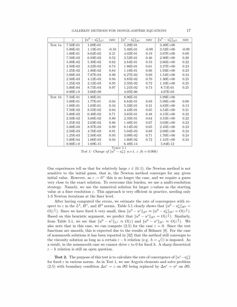
Test 1:. For this test, we calculate ‖u0 − uεh‖ for fixed h = 0.009, while varyingε in order to approximate the error ‖uε − u0‖. We use Argyris elements and set tosolve problem (2.5) with the following test functions:

(a). u0 = e(x2+y2)/2, f = (1 + x2 + y2)e(x2+y2)/2, g = e(x2+y2)/2.

(b). u0 = x4 + y2, f = 24x2, g = x4 + y2.


ε ‖u0 − uεh‖L2 rate ‖u0 − uε

h‖H1 rate ‖u0 − uεh‖H2 rate

Test 1a 7.50E-01 1.09E-01 5.29E-01 3.40E+005.00E-01 1.13E-01 -0.10 5.48E-01 -0.09 3.52E+00 -0.091.00E-01 8.04E-02 0.21 4.02E-01 0.19 3.07E+00 0.097.50E-02 6.93E-02 0.52 3.52E-01 0.46 2.90E+00 0.205.00E-02 5.39E-02 0.62 2.84E-01 0.53 2.66E+00 0.222.50E-02 3.22E-02 0.74 1.86E-01 0.61 2.27E+00 0.231.25E-02 1.80E-02 0.84 1.18E-01 0.66 1.93E+00 0.235.00E-03 7.87E-03 0.90 6.27E-02 0.69 1.54E+00 0.242.50E-03 4.12E-03 0.94 3.85E-02 0.70 1.30E+00 0.251.25E-03 2.12E-03 0.95 2.35E-02 0.72 1.10E+00 0.255.00E-04 8.75E-04 0.97 1.21E-02 0.73 8.71E-01 0.250.00E+0 3.66E-09 4.05E-06 4.07E-03

Test 1b 7.50E-01 1.80E-01 8.96E-01 5.99E+005.00E-01 1.77E-01 0.04 8.84E-01 0.03 5.98E+00 0.001.00E-01 1.03E-01 0.34 5.33E-01 0.31 4.82E+00 0.137.50E-02 8.55E-02 0.64 4.43E-01 0.65 4.54E+00 0.215.00E-02 6.40E-02 0.71 3.65E-01 0.48 4.15E+00 0.222.50E-02 3.68E-02 0.80 2.35E-01 0.64 3.55E+00 0.221.25E-02 2.03E-02 0.86 1.48E-01 0.67 3.03E+00 0.235.00E-03 8.97E-03 0.89 8.14E-02 0.65 2.45E+00 0.232.50E-03 4.76E-03 0.91 5.04E-02 0.69 2.08E+00 0.241.25E-03 2.50E-03 0.93 3.09E-02 0.71 1.76E+00 0.245.00E-04 1.06E-03 0.94 1.60E-02 0.72 1.41E+00 0.240.00E+0 1.69E-15 6.48E-14 5.84E-12

Table 5.1Test 1: Change of ‖u0 − uε

h‖ w.r.t. ε (h = 0.009)

Our experiences tell us that for relatively large ε ∈ (0, 1), the Newton method is notsensitive to the initial guess, that is, the Newton method converges for any giveninitial value. However, as ε → 0+ this is no longer the case, and we require a guessvery close to the exact solution. To overcome this burden, we use a multi-resolutionstrategy. Namely, we use the numerical solution for larger ε-values as the startingvalue at a finer resolution ε. This approach is very efficient in practice, needing only1-3 Newton iterations at the finer level.

After having computed the errors, we estimate the rate of convergence with re-spect to ε in the L2, H1, and H2 norms. Table 5.1 clearly shows that ‖u0 − uεh‖H2 =O(ε

14 ). Since we have fixed h very small, then ‖u0 − uε‖H2 ≈ ‖u0 − uεh‖H2 = O(ε

14 ).

Based on this heuristic argument, we predict that ‖u0 − uε‖H2 = O(ε14 ). Similarly,

from Table 5.1, we see that ‖u0 − uε‖L2 ≈ O(ε) and ‖u0 − uε‖H1 ≈ O(ε34 ). We

also note that in this case, we can compute (2.5) for the case ε = 0. Since the testfunctions are smooth, this is expected due to the results of Bohmer [8]. For the caseof nonsmooth solutions it has been reported in [32] that the method still converges tothe viscosity solution as long as a certain ε− h relation (e.g. h =

√ε) is imposed. As

a result, in the nonsmooth case we cannot drive ε to 0 for fixed h. A sharp theoreticalε− h relation is still an open question.

Test 2. The purpose of this test is to calculate the rate of convergence of ‖uε−uεh‖for fixed ε in various norms. As in Test 1, we use Argyris elements and solve problem(2.5) with boundary condition ∆uε = ε on ∂Ω being replaced by ∆uε = φε on ∂Ω.


h ‖uε − uεh‖L2 rate ‖uε − uε

h‖H1 rate ‖uε − uεh‖H2 rate

Test 2a 8.33E-02 4.10E-05 2.69E-03 1.70E-015.00E-02 1.08E-06 7.11 9.92E-05 6.46 1.17E-02 5.243.07E-02 3.65E-08 6.93 5.43E-06 5.94 9.86E-04 5.052.38E-02 7.67E-09 6.21 1.29E-06 5.71 3.13E-04 4.571.60E-02 4.51E-10 7.09 1.09E-07 6.19 4.04E-05 5.131.28E-02 8.88E-11 7.38 2.44E-08 6.80 1.19E-05 5.56

Test 2b 8.33E-02 2.11E-08 4.92E-07 4.17E-055.00E-02 5.17E-10 7.26 1.90E-08 6.37 2.72E-06 5.343.07E-02 1.77E-11 6.90 1.05E-09 5.93 2.40E-07 4.962.38E-02 3.60E-12 6.34 2.62E-10 5.50 7.51E-08 4.621.60E-02 2.03E-13 7.19 2.24E-11 6.16 9.52E-09 5.171.28E-02 3.64E-14 7.81 4.96E-12 6.85 2.70E-09 5.73

Table 5.2Test 2: Change of ‖uε − uε

h‖ w.r.t. h (ε = 0.001)

We use the following test functions:

(a). uε = 20x6 + y6, fε = 18000x4y4 − ε(7200x2 + 360y2),

gε = 20x6 + y6, φε = 600x4 + 30y4.

(b.) uε = x sinx+ y sin y, fε = (2 cosx− x sinx)(2 cos y − y sin y)− ε(x sinx− 4 cosx+ y sin y − 4 cos y),

gε = x sinx+ y sin y, φε = 2 cosx− x sinx+ 2 cos y − y sin y.

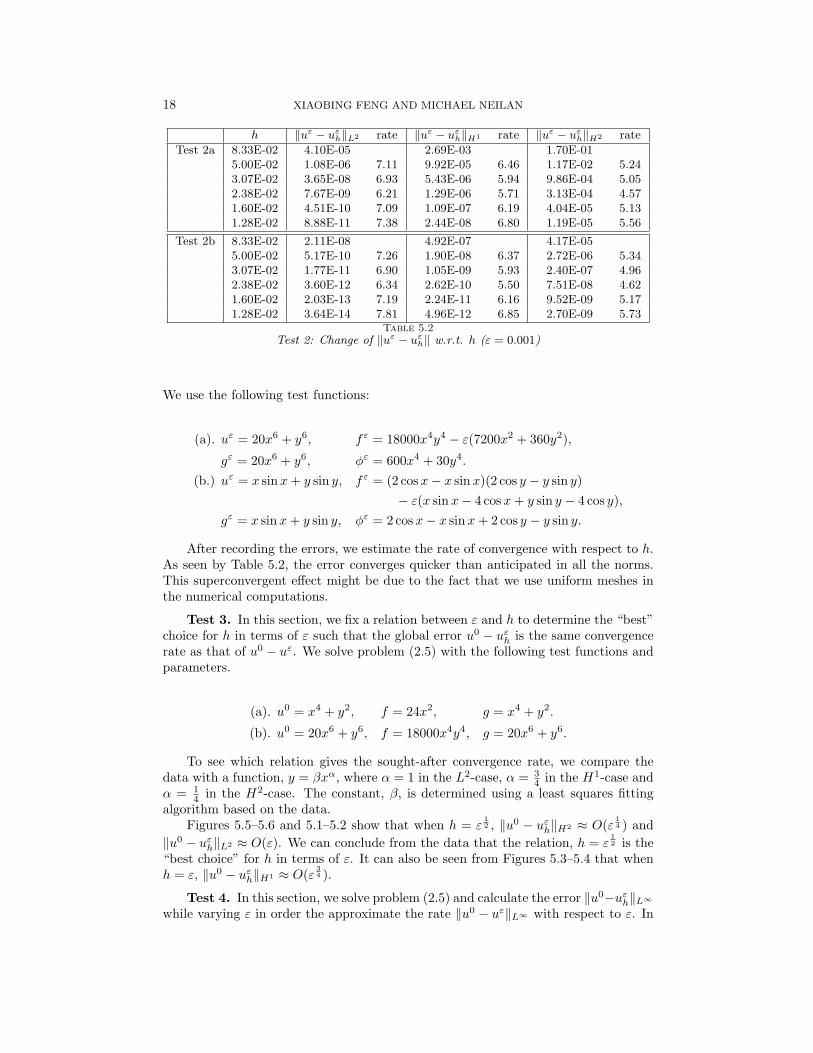
After recording the errors, we estimate the rate of convergence with respect to h.As seen by Table 5.2, the error converges quicker than anticipated in all the norms.This superconvergent effect might be due to the fact that we use uniform meshes inthe numerical computations.

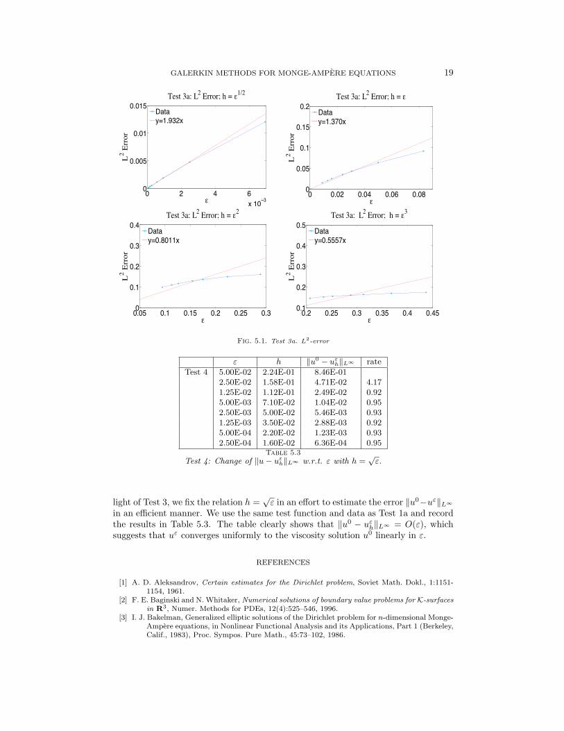
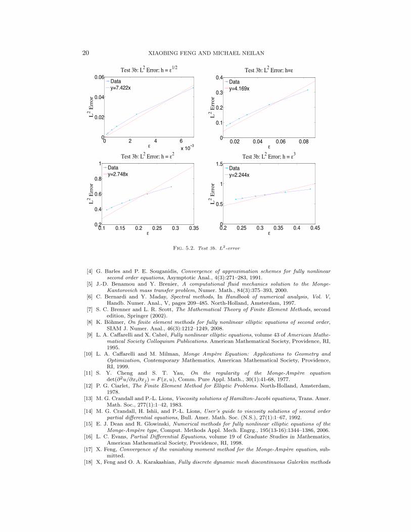
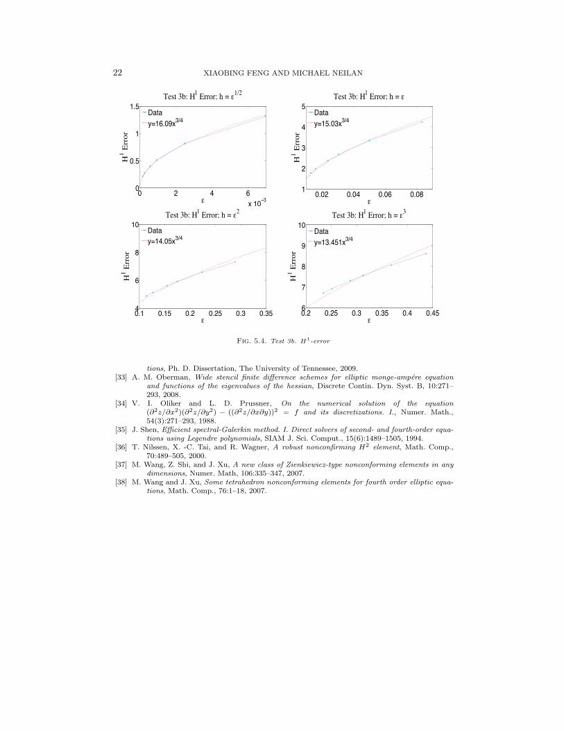
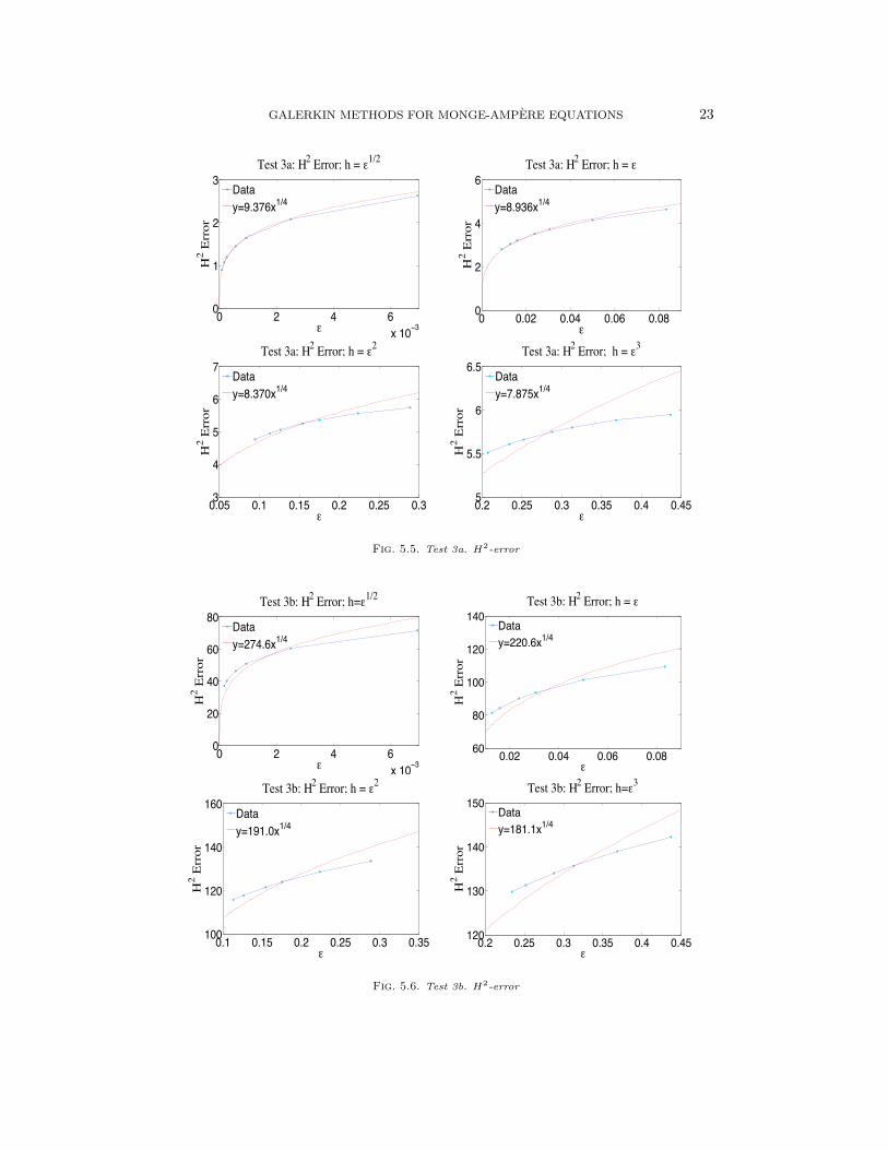
Test 3. In this section, we fix a relation between ε and h to determine the “best”choice for h in terms of ε such that the global error u0 − uεh is the same convergencerate as that of u0 − uε. We solve problem (2.5) with the following test functions andparameters.

(a). u0 = x4 + y2, f = 24x2, g = x4 + y2.

(b). u0 = 20x6 + y6, f = 18000x4y4, g = 20x6 + y6.

To see which relation gives the sought-after convergence rate, we compare thedata with a function, y = βxα, where α = 1 in the L2-case, α = 3

4 in the H1-case andα = 1

4 in the H2-case. The constant, β, is determined using a least squares fittingalgorithm based on the data.

Figures 5.5–5.6 and 5.1–5.2 show that when h = ε12 , ‖u0 − uεh‖H2 ≈ O(ε

14 ) and

‖u0 − uεh‖L2 ≈ O(ε). We can conclude from the data that the relation, h = ε12 is the

“best choice” for h in terms of ε. It can also be seen from Figures 5.3–5.4 that whenh = ε, ‖u0 − uεh‖H1 ≈ O(ε

34 ).

Test 4. In this section, we solve problem (2.5) and calculate the error ‖u0−uεh‖L∞while varying ε in order the approximate the rate ‖u0 − uε‖L∞ with respect to ε. In


0 2 4 6x 10−3

0

0.005

0.01

0.015Test 3a: L2 Error; h = !1/2

!

L2 E

rror

Datay=1.932x

0 0.02 0.04 0.06 0.080

0.05

0.1

0.15

0.2Test 3a: L2 Error; h = !

!

L2 E

rror

Datay=1.370x

0.05 0.1 0.15 0.2 0.25 0.30

0.1

0.2

0.3

0.4Test 3a: L2 Error; h = !2

!

L2 E

rror

Datay=0.8011x

0.2 0.25 0.3 0.35 0.4 0.450.1

0.2

0.3

0.4

0.5Test 3a: L2 Error; h = !3

!

L2 E

rror

Datay=0.5557x

Fig. 5.1. Test 3a. L2-error

ε h ‖u0 − uεh‖L∞ rate

Test 4 5.00E-02 2.24E-01 8.46E-012.50E-02 1.58E-01 4.71E-02 4.171.25E-02 1.12E-01 2.49E-02 0.925.00E-03 7.10E-02 1.04E-02 0.952.50E-03 5.00E-02 5.46E-03 0.931.25E-03 3.50E-02 2.88E-03 0.925.00E-04 2.20E-02 1.23E-03 0.932.50E-04 1.60E-02 6.36E-04 0.95

Table 5.3Test 4: Change of ‖u− uε

h‖L∞ w.r.t. ε with h =√

ε.

light of Test 3, we fix the relation h =√ε in an effort to estimate the error ‖u0−uε‖L∞

in an efficient manner. We use the same test function and data as Test 1a and recordthe results in Table 5.3. The table clearly shows that ‖u0 − uεh‖L∞ = O(ε), whichsuggests that uε converges uniformly to the viscosity solution u0 linearly in ε.

REFERENCES

[1] A. D. Aleksandrov, Certain estimates for the Dirichlet problem, Soviet Math. Dokl., 1:1151-1154, 1961.

[2] F. E. Baginski and N. Whitaker, Numerical solutions of boundary value problems for K-surfacesin R3, Numer. Methods for PDEs, 12(4):525–546, 1996.

[3] I. J. Bakelman, Generalized elliptic solutions of the Dirichlet problem for n-dimensional Monge-Ampere equations, in Nonlinear Functional Analysis and its Applications, Part 1 (Berkeley,Calif., 1983), Proc. Sympos. Pure Math., 45:73–102, 1986.


0 2 4 6x 10−3

0

0.02

0.04

0.06Test 3b: L2 Error; h = !1/2

!

L2 E

rror

Datay=7.422x

0.02 0.04 0.06 0.080

0.1

0.2

0.3

0.4Test 3b: L2 Error; h=!

!

L2 E

rror

Datay=4.169x

0.1 0.15 0.2 0.25 0.3 0.350.2

0.4

0.6

0.8

1Test 3b: L2 Error; h = !2

!

L2 E

rror

Datay=2.748x

0.2 0.25 0.3 0.35 0.4 0.450

0.5

1

1.5Test 3b: L2 Error; h = !3

!

L2 E

rror

Datay=2.244x

Fig. 5.2. Test 3b. L2-error

[4] G. Barles and P. E. Souganidis, Convergence of approximation schemes for fully nonlinearsecond order equations, Asymptotic Anal., 4(3):271–283, 1991.

[5] J.-D. Benamou and Y. Brenier, A computational fluid mechanics solution to the Monge-Kantorovich mass transfer problem, Numer. Math., 84(3):375–393, 2000.

[6] C. Bernardi and Y. Maday, Spectral methods, In Handbook of numerical analysis, Vol. V,Handb. Numer. Anal., V, pages 209–485. North-Holland, Amsterdam, 1997.

[7] S. C. Brenner and L. R. Scott, The Mathematical Theory of Finite Element Methods, secondedition, Springer (2002).

[8] K. Bohmer, On finite element methods for fully nonlinear elliptic equations of second order,SIAM J. Numer. Anal., 46(3):1212–1249, 2008.

[9] L. A. Caffarelli and X. Cabre, Fully nonlinear elliptic equations, volume 43 of American Mathe-matical Society Colloquium Publications. American Mathematical Society, Providence, RI,1995.

[10] L. A. Caffarelli and M. Milman, Monge Ampere Equation: Applications to Geometry andOptimization, Contemporary Mathematics, American Mathematical Society, Providence,RI, 1999.

[11] S. Y. Cheng and S. T. Yau, On the regularity of the Monge-Ampere equationdet(∂2u/∂xi∂xj) = F (x, u), Comm. Pure Appl. Math., 30(1):41-68, 1977.

[12] P. G. Ciarlet, The Finite Element Method for Elliptic Problems. North-Holland, Amsterdam,1978.

[13] M. G. Crandall and P.-L. Lions, Viscosity solutions of Hamilton-Jacobi equations, Trans. Amer.Math. Soc., 277(1):1–42, 1983.

[14] M. G. Crandall, H. Ishii, and P.-L. Lions, User’s guide to viscosity solutions of second orderpartial differential equations, Bull. Amer. Math. Soc. (N.S.), 27(1):1–67, 1992.

[15] E. J. Dean and R. Glowinski, Numerical methods for fully nonlinear elliptic equations of theMonge-Ampere type, Comput. Methods Appl. Mech. Engrg., 195(13-16):1344–1386, 2006.

[16] L. C. Evans, Partial Differential Equations, volume 19 of Graduate Studies in Mathematics,American Mathematical Society, Providence, RI, 1998.

[17] X. Feng, Convergence of the vanishing moment method for the Monge-Ampere equation, sub-mitted.

[18] X, Feng and O. A. Karakashian, Fully discrete dynamic mesh discontinuous Galerkin methods


0 2 4 6x 10−3

0

0.05

0.1

0.15

0.2Test 3a: H1 Error; h = !1/2

!

H1 E

rror

Datay=0.9942x3/4

0 0.02 0.04 0.06 0.080

0.2

0.4

0.6

0.8Test 3a: H1 Error; h = !

!

H1 E

rror

Datay=1.565x3/4

0.05 0.1 0.15 0.2 0.25 0.30.2

0.4

0.6

0.8

1Test 3a: H1 Error; h = !2

!

H1 E

rror

Datay=1.684x3/4

0.2 0.25 0.3 0.35 0.4 0.45

0.8

1

1.2

1.4Test 3a: H1 Error; h = !3

!

H1 E

rror

Datay=1.516x3/4

Fig. 5.3. Test 3a. H1-error

for the Cahn-Hilliard equation of phase transition, Math. Comp. 76:1093–1117, 2007.[19] X. Feng and M. Neilan, The vanishing moment method for fully nonlinear second order PDEs:

formulation, theory, and numerical analysis, submitted.[20] X. Feng and M. Neilan, Vanishing moment method and moment solutions for second order

fully nonlinear partial differential equations, J. Scient. Comp., 38:74–98, 2009.[21] X. Feng and M. Neilan, Mixed finite element methods for the fully nonlinear Monge-Ampere

equation based on the vanishing moment method, SIAM J. Numer. Anal., 47:1226–1250,2009.

[22] X. Feng, M. Neilan, and A. Prohl, Error analysis of finite element approximations of theinverse mean curvature flow arising from the general relativity, Numer. Math., 108(1):93-119, 2007.

[23] W. H. Fleming and H. M. Soner, Controlled Markov processes and viscosity solutions, volume 25of Stochastic Modelling and Applied Probability. Springer, New York, second edition, 2006.

[24] D. Gilbarg and N. S. Trudinger, Elliptic Partial Differential Equations of Second Order, Classicsin Mathematics, Springer-Verlang, Berlin, 2001. Reprint of the 1998 edition.

[25] C. E. Gutierrez, The Monge-Ampere Equation, volume 44 of Progress in Nonlinear DifferentialEquations and Their Applications, Birkhauser, Boston, MA, 2001.

[26] P. Grisvard Elliptic Problems in Nonsmooth Domains, Pitman (Advanced Publishing Pro-gram), Boston, MA, 1985.

[27] H. Ishii, On uniqueness and existence of viscosity solutions of fully nonlinear second orderPDE’s, Comm. Pure Appl. Math., 42:14–45, 1989.

[28] R. Jensen, The maximum principle for viscosity solutions of fully nonlinear second order partialdifferential equations, Arch. Rational Mech. and Anal., 101:1–27, 1988.

[29] O. A. Ladyzhenskaya and N. N. Ural’tseva, Linear and Quasilinear Elliptic Equations, Aca-demic Press, New York, 1968.

[30] R. J. McCann and A. M. Oberman. Exact semi-geostrophic flows in an elliptical ocean basin,Nonlinearity, 17(5):1891–1922, 2004.

[31] I. Mozolevski and E. Suli, A priori error analysis for the hp-version of the discontinuousGalerkin finite element method for the biharmonic equation, Comput. Meth. Appl. Math.3:596–607, 2003.

[32] M. Neilan, Numerical Methods for Fully Nonlinear Second Order Partial Differential Equa-


0 2 4 6x 10−3

0

0.5

1

1.5Test 3b: H1 Error; h = !1/2

!

H1 E

rror

Datay=16.09x3/4

0.02 0.04 0.06 0.081

2

3

4

5Test 3b: H1 Error; h = !

!

H1 E

rror

Datay=15.03x3/4

0.1 0.15 0.2 0.25 0.3 0.354

6

8

10Test 3b: H1 Error; h = !2

!

H1 E

rror

Datay=14.05x3/4

0.2 0.25 0.3 0.35 0.4 0.456

7

8

9


!

H1 E

rror

Datay=13.451x3/4

Fig. 5.4. Test 3b. H1-error

tions, Ph. D. Dissertation, The University of Tennessee, 2009.[33] A. M. Oberman, Wide stencil finite difference schemes for elliptic monge-ampere equation

and functions of the eigenvalues of the hessian, Discrete Contin. Dyn. Syst. B, 10:271–293, 2008.

[34] V. I. Oliker and L. D. Prussner, On the numerical solution of the equation(∂2z/∂x2)(∂2z/∂y2) − ((∂2z/∂x∂y))2 = f and its discretizations. I., Numer. Math.,54(3):271–293, 1988.

[35] J. Shen, Efficient spectral-Galerkin method. I. Direct solvers of second- and fourth-order equa-tions using Legendre polynomials, SIAM J. Sci. Comput., 15(6):1489–1505, 1994.

[36] T. Nilssen, X. -C. Tai, and R. Wagner, A robust nonconfirming H2 element, Math. Comp.,70:489–505, 2000.

[37] M. Wang, Z. Shi, and J. Xu, A new class of Zienkiewicz-type nonconforming elements in anydimensions, Numer. Math, 106:335–347, 2007.

[38] M. Wang and J. Xu, Some tetrahedron nonconforming elements for fourth order elliptic equa-tions, Math. Comp., 76:1–18, 2007.


0 2 4 6x 10−3

0

1

2

3Test 3a: H2 Error; h = !1/2

!

H2 E

rror

Datay=9.376x1/4

0 0.02 0.04 0.06 0.080

2

4

6Test 3a: H2 Error; h = !

!

H2 E

rror

Datay=8.936x1/4

0.05 0.1 0.15 0.2 0.25 0.33

4

5

6

7Test 3a: H2 Error; h = !2

!

H2 E

rror

Datay=8.370x1/4

0.2 0.25 0.3 0.35 0.4 0.455

5.5

6

6.5Test 3a: H2 Error; h = !3

!

H2 E

rror

Datay=7.875x1/4

Fig. 5.5. Test 3a. H2-error

0 2 4 6x 10−3

0

20

40

60

80Test 3b: H2 Error; h=!1/2

!

H2 E

rror

Datay=274.6x1/4

0.02 0.04 0.06 0.0860

80

100

120

140Test 3b: H2 Error; h = !

!

H2 E

rror

Datay=220.6x1/4

0.1 0.15 0.2 0.25 0.3 0.35100

120

140


!

H2 E

rror

Datay=191.0x1/4

0.2 0.25 0.3 0.35 0.4 0.45120

130

140

150Test 3b: H2 Error; h=!3

!

H2 E

rror

Datay=181.1x1/4

Fig. 5.6. Test 3b. H2-error

analysis of galerkin methods for the fully

Documents