Analysis of geometrically non-linear bending of beamsand plates with mixed-type finite elementsMenken, C.M.

DOI:10.6100/IR5248

Published: 01/01/1974

Document VersionPublisher’s PDF, also known as Version of Record (includes final page, issue and volume numbers)

Please check the document version of this publication:

• A submitted manuscript is the author's version of the article upon submission and before peer-review. There can be important differencesbetween the submitted version and the official published version of record. People interested in the research are advised to contact theauthor for the final version of the publication, or visit the DOI to the publisher's website.• The final author version and the galley proof are versions of the publication after peer review.• The final published version features the final layout of the paper including the volume, issue and page numbers.

Link to publication

Citation for published version (APA):Menken, C. M. (1974). Analysis of geometrically non-linear bending of beams and plates with mixed-type finiteelements Eindhoven: Technische Hogeschool Eindhoven DOI: 10.6100/IR5248

General rightsCopyright and moral rights for the publications made accessible in the public portal are retained by the authors and/or other copyright ownersand it is a condition of accessing publications that users recognise and abide by the legal requirements associated with these rights.

• Users may download and print one copy of any publication from the public portal for the purpose of private study or research. • You may not further distribute the material or use it for any profit-making activity or commercial gain • You may freely distribute the URL identifying the publication in the public portal ?

Take down policyIf you believe that this document breaches copyright please contact us providing details, and we will remove access to the work immediatelyand investigate your claim.

Download date: 16. May. 2018

ANALYSIS

OF GEOMETRICALLY NON-LINEAR

BENDING OF BEAMS

AND PLATES WITH MIXED-TYPE

FINITE ELEMENTS

PROEFSCHRIFT

~er verkrij~ing van de gr~~d Van do(to~ in de

~echnis~he wetensch~ppen aan de T~chnischc

Hogeschool Eindhoven. op gezag van de rector

magnificu~~ prof.dr,ir, G. Vo~~eL~~ voar ~en

cOmMi~Sie aangewezen door ne~ ~o11ege van

dekan@n in het openbaar te verdedigen op

dinsdag 26 maart 1974 te 16.00 uur

door

Carnelis Marinus Menken gebo~en te Haarlem

1 E C H N I S C H E HOG ESC H 0 0 LEI N D H 0 V E N

DIT PROEFSCHRIFT IS GOWGEKEUKD

DOOR Die PROMOTOR£N

PROF,DR,TR, J,D, JANSSEN

en

PROF.DK. J,ll. ALBLAS

Aan: Riet

Lieeb$th

Karin

Marijl<e

CONTENTS

Introduc tion •••••••.•....•..•...••••••.•••.•..•.......•••••...• 9

Chapt~r I, The relation of Herrmann's variationaL principl~ to .•

other v~riatiorta.l principles ...... ,. +, ••••• ". I I •• I I I ... , t, .• t. 15

1 • 1 Introd,-,,, tion •....•••••••••••••••••••.....•••••••••••. ,.. IS

1,2 General transformation scheme •••••••••••• , .. ,...... ..... 16

1.3 The relation of Herrmann's vari~t~onal principle to ••.••

other variational principles •••••••••• ,................. 21

Chapter 2, Exten~ion of Herrmann's variational principle for

the case of geometrically non-linear bending of beams 28

2.1 Introduction •••••• , ••••••••.......••.•••.•..•. ,......... 28

2.2 Potential ener$Y formulation for geometrically non-linear

bending of beam~, including the effect of tranverse shear

deformation •••• , •. , .....••.•••••••••••••• ,.............. 29

2.3 Forces and moment of the cross-section, ~nd beam equations 35

2.4 Oerivation of Herrmann's variational principle ~n ca~e of

geometrically non-linear bending of beams •..•.••.••••••• 39

2.5 Correctness of the formulation •••••••••••• ,.,',... ...•.• 42

Chapter 3, Some procedures for obtain~ng finite element mooels. 45

3. I lntroduction .•..••.•• , ..••.•............•• ,............. 45

3.Z The finite-element method and COnvergence criteria 46

3.3 Some alternative finite-element procedures as ~seo in tne

st~tionary potential energy approach ......••••••••••••.. 48

3.4 Alternativ~ finite-element procedures for the Herrmann ..

form1,l1ation 53

3.5 A finite-element formulation for large displacement of .•

beams ..•..••.•..• , .••.•..•. , •. ,.,.,..................... 56

3,6 Numerical examples ...................................... 61

7

Chapter 4, Derivation of the Herrmann formulation for the an~-

lysis of finite defl~ctiong of plates. •.••• .•.... ...... ••. 68

4. I Introduc tion ......•....•.•.•••••••.•.••............... 68

4.2 The potential eneJ:"8Y form\llation suited to H,e trart~for-

m8.tion to the lierrmann formuLation . ~.................. 69

4.3 Derivation of the Herrmann formulation .. ...... ....• ••• 76

11,4 Corre,c:.tn-e$F.i of the formulation ........ r ........ wi. I ..... I 78

4.5 Alternative finite-element models ....... .............. 80

Chapter 5, A mixed finite element for the analysis of plate ••

bending

5.1 Introduction ..••.•••••••.•••••••••••••••••••••.•...... 86

5.2 Formulation of the finitE-element model............... 86

5.3 The cont.ribution of prescribed loads and rotations.... 100

5.4 The contribution of One element to the non-linear ...•.

equations of the entire structure 101

5.5 The contrihution of an element to the incremental .....

equations of the entire scructure 104

Chapter 6~ Th~ ~quation5 of the entire structur~t the CO~puter

program and B nl.,lmeriC,::I:l example '" f +. I .. I I f "" I .... I .. + 1+.. • •• • •• 106

6.1 Tntroduction .......................................... 106

6.2 Tha ~quations of tha Qntir~ structur~ ... .•• .••.•• .•.•• 106

6.3 Ihe tomput~r program 114

0.4 Numerical example...... .......... ....... ..... ......... 121

S,lmmary and conclusions ...................................... I 129

Appendix A~ Equation~ of the finite di~placernent theory of ...

e 1 a 5 tic it y ..... , .............. I •• I I ••• I .. I •• I I .................... I I 1 ."34

Appendix B, Numerical solution of set~ of non-linear ",quations 1.)8

Appendi.x C, Indentification of the multipliers occuring in the

plate formulation......................................... 142

Appendix D, Auxiliary relations referred to in Chapter 5 •• ••• 147

Notation 150

References .......•••.••••.•••••••••••••••••••••••••••.••••••• 158

8

iNTRODUCTION

During the last few ~eca~es the Einit~-element methods have

proved to be useful engineering tool~ for th~ analysis of a great

variety of structures.

,ni"ially the developments we~e con~ined to linea~ theo~ies, and

e~pecial1y after reCOurse had been had to the p~inciple of minimum

potential ene~gy for the gene~~tion of finite-element models, the

displacement method based on this principle wa~ widely accepted.

Finite elements formulated conforming to the ~equirements of

this principle are said to be consistent, while in that case the dis­

placement forwulation becomes a pa~ticular case of the Rit~ method so

that Lhe cOnVerSence theory of the latter can be applied~

A great number of elements has since been developed for the ana­

lysis of ditferent classes of structures. In the case of plate ben­

ding, however, it p~oved difficul" to formulate consistent triangula~

elements oeca~se the follo~ing requi.ements had to be fulfilled at

the same time :

along ~a~h ~id~ both the lat~ral di,placement and the rotations of

the normals to the middle plane eho~ld be compatible

- tne properties of the element eho~ld be independent of the choice

of the coordinate system. ~~en describing th~ displac~ment distri­

b~tion by means of polynomial~, this can only be ac~ompli5hed by

~6ing complete polynomials.

Attention i5 here devoted to triangular e.l~ment;:s sipce these. permit

the representation of complicated plat~ ~onfigurations.

9

CLOUGH and TOCHER I bave presented an evaluation of s\l<;h ele­

ments. The major existing approaches are:

- to r"nounce the comp,qtibility of the normal rotations 2. OLIVEIRA]

proved that in that C0se no conve~gence can be obtained unless the

elements (ire so ol-tt'(inged that the nodes are all of the Eame kind;

i.e. surrounded in the same way by ~lam~nt£. This restricts the

applicability considerably;

- to te-establish compatibility by m~ans of correcrion functions 4.

Strange enOugh, this adve~sely influenced thR spe~d of convergence

which, tifter all .. was e.xpected to -i.n.cre~"lse;

- to use nigner-order pol ynomi.als CfUth degree) for the displace­

ments and introducin~ curvatures and twisting as degTees of fre~-5 6 .. .'

dom '. ThlS lmpbes special provisions if el,emencs with diffe-

ring thicknesses are coupl~d to e<lch other and if at edges neith~r

the deflection nor the rotation are specified. Moreover, a large

number of degrees oI freedom (18) is involved;

- oy d ivid i.ne the element into subregions. assuming independent poly­

nomial di~placement distributions for each subelement and requiring

compatibility between the 6ubelemenC$ 7

A.~ incomplete polynonlials are used, the properties of the element

become dependent on the .;holce of the. coordin<lte system. CLOlJGH and

TOCHER I and CLOUGH <Ind fELIPPA 8 have presented " complicated

quadrilateral element the def.lection of which is expressed by

expansions over twelve tri"ngutar subregions. Acoording to CLOUGH 9

the development o~ this element took seve:r;/il years.

The approaches mentioned above are not meant as a chorough evalua­

tion of existing plate bending elements but merely as an indication

of tne difficultieB encountered when t1:ying to formulate triangular

plat~-bending element~ cOnsi5ten~ with the principle of minimum

potential energy.

Another disadvantage of the latter formulation is that, apart

froIII the deflections. in may ca$es one is inte1:ested in th~ b(!l'Iding

10

atresseS. Since in the relevant principle the stress-strain rela­

tions and the strain-displace~ent r~lationa are assumed to be known,

the commonly rollowed way is to use thes~ to ~alculate the stresses

from the approximated diapla~ementa. In the plate bending theory,

however, this means that the bending stresses are related to the

second derivatives o£ the approximated deflection and thus will be

rather inaccurate, especially when using simple polynomials. More­

over, these stresses are discontinuous at the element boundaries

since equilibrium is only satisfied in the mean.

Other wayS of stress calculation, such as redistributing the

generali~ed torces over the edges of the element 6 or using the

theory of conjugate approximations to constru~t continuous atress

approximations 10 are not widely used.

In 1965, HER~NN l I p~esented a variational printiple to COn~ 3tr~ct approximat~ ~olutions for plat~ b~nding probl~m~ that offered

a very attractive solution to the aforemention~d problems since both

deflection ~nd moments appear a~ the unknowns in the formulation.

The less int~r~Bting rotations and shear forces are related to these

unknows by first derivates. At the element interfaces th~ only re~

quirement made on the unknowns i~ continuity, so that the diffi~ulty

of fulfilling rotation continuity is not ~ncountered. In consequence,

simple polynomia~s c~n be used.

Although the principle was not a minimum principle, OLIVEIRA 3

has formulated the convergence c~iteria.

The simple functional form of the deflection can ~lso be used

for the in-plane displacements, thus enabling the an!!lysis of folded

plate structur~s to be made.

During the last few years the finite-element method has also

been extended to a great variety of non-,inear problems. In this

thesis attention will be giv~n to geometrically non-linear plate

bending problems, which meanS that the deflections are of such mag­

nitude that linearization of the strain-displacement relationship ~s

not justifiable.

II

The first work on the extension to geometrical non-line&rity

was reported by TURNER et ,,1 13, In a subsequent paper, GALLAGHER et

a1 14 outlined a conststenc procedure, based on the principle of

minimum potel1ti'~1 ellel.""gy for }'Dtrodl.J.cing the geomet;:rf~al n0l,1-1 ineari­

ty in t))~ pertinent fini.te-element displ,'cement formu),ation,

MALLF:r ~n(i MAR~AL 15 have preHnted a summary of the developments in

this field.

Still more than i.n th() case of the liIlear formulations the de­

velopments were based on the principle of stationary potential ener­

gy. probably because this displacement formulati.on had already been

widel y accepted when solving linear problems. Moreover, a <) i.splace­

ment formulation looks the most appropriate to iIlcorporate the geo­

metrical non-linea<ity.

However. when developing consistent elements for geometrically

nDn-lin~ar plate bendiIlg along this line, the same problems as met in

the linear fotmuletion appear. Thus it looked very attraetive to make

use of the .jIdvantages of Herrmann's formulation also in the large de­

flection range. To that aIld, Herrmann's principIa should be e~rended

to geomet<ically ncn-linear bending.

The <'''tension of othe~ variational principles being known, the

extenBion of Herrm(lnn's pJ:"inciple seemed feasible. For instance, the

following exten~ion~ (Ire known:

The extension of the princi.ple of minimum potential energy to 1,~rBe

deformations as given by KAPPUS 16

- RE1SSNER's variation,,! principle (IS e"tendeo by RElS5NER himself 18

- Hu-wAsH12u's principle 19 as ""tended by TEREC;ULOV 20 ZI 22

For the geometrical non~linear case ZUBOV and KOlTER have

recently taken Rignificant steps towards effect~ve generalization

of the principle of cDmplementary anergy.

These exten~i.oTl~ being establi~hed, the question remains how

they can be obtained systematically.

12

In the li~ear domain chere exists a general c~~n6formatio~

scheme, known as FRIEDRICHS'transfo~mation, which makes possible the

cransformation of a potentional energy formulatio~ in co a compleme~­

tary energy formulation by a set of ~ell-defined steps. Other formu­

lations, su~h as R~ISSNER's, sre obtainable as intermediate steps.

Whereas the sbove publications o~ extended variational pri~ei­

pIes offer ~o information on how they have bee~ derived, wASHIZij 23

derived them by proceeding along the same lines as in the li~ear

theory.

Up co nOw, however, with the ex~eption of the potential energy

formulation, the extended principles seem not to have been followed

up by an implementation in fi~ite-element models.

Therefore, the main obje~tives of the present thesis have been

formulatea as follows:

I, TO establish the relationship of Herrmann's v~~iational prin~ipl~

with other existing variatio~al p~inciple~,

2, To use this r~lationship to extend Herrmann's variational prin­

ciple to the particular cas~ where the strain-displa~ement rela­

Lions are not linear,

3. To develop a computer program for the analysi.s of geometrically

no~-linear bending of plates based on this extended variational

principle.

The following approach will be used:

The place of Herrmann's variational prin~iple in FriedriChs'

transformation scheme will be determined. This pl~ce being known,

the steps to be taken to create this principle from a ~iven poten­

ti~l energy formulation are defi~ed, This will be illustrated for

the mathematically simple e~ample of a cantilever beam (Chapte~ I).

13

StHting e1:"om the potential energy fOT!l)tIlation for the small­

otr<:lins large-displacement theory of elastic 1)",am~. the same steps

~r" to b~ used to generate the extended Hen-mann formulation for this

problem. The Euler equatiortG of th" latter are compared with the

BoverninB field equations to prov~. the validity of the new formula­

tion (Chapter 2).

Moreover, .some numet"ictil :results obtait'l.cd with a cons.istent

finite element formulation will be presented (Chapter J).

By analogy, starting from th~_ potenti a1 energy formulat ion for

the VOn Karman plate bending cheery, the Herrmann formulation of

this th(!ory will be dedved (Chapter 4),

A tomputer program will be developed for the approximate solu­

tiOn to finit" plate b"l'lding by means of the finite eleme.nt method,

hased on thi. extended Herrmann formulation (Chapters 5 and 6).

Although a geometrical non-linear formulation implies the possi­

bility of buckling analysis, the latter 5ubject~ will not be treated

in t.hi~ thef! i_<;:,

14

CHAPTER I

The relauon of Herrmann's variational principle to other variational principles

1.1 Introduction

In the cl~b5ical linear theory of elasticity a general scheme

exists (e.g.2.1) making possible the generation of differen~ varia­

tional principles by starting from a kno~ potential energy formu­

lation and proceeding by taking ~ome well-cte£ined steps.

The aim being to formulate Herrmann'S variational prin~iple for

geometrically non~linear analy~i~ of beam~ and plates and the rele­

vant potential energy formulation being known, it seemed worthwile

to determine the place of the existing Herrmann's principle in this

scheme. When this plac@ is known, the steps to be taken to generate

the Herrmann formulation from the potential energy formulation are

defined for the linear case.

Subsequently, by starting from the potential energy formulation

for the geometrically non~linear case and taking the same steps, the

Herr~anrt formultition extended to the geometrically non-linear case

will be obtained.

In this Chapter the relation of the existing Herrmann formula­

tion with other variational formulation~ wi~l be determined.

In SectiOn 1,2 the general transforma<lon scheme, known a~

Friedriche'transformation, will be 5umrnsri~ed,

In Section 1.3 it will be shown that Herrmann's principle is

partly a potential energy prin~iple and partly a complementary prin­

ciple, and ~an be s£nerat£d from a fully potential energy formula­

tion by applying the Friedrichs'transformation.

15

The argvment. will b~ illu.trateO by means of the mathematically

simple example of a cantilever beam.

A general thr~e-diman.ional elaboration i. not practical since in

a specifi( "ending probl~m the separate stress-displacement systems

to be treateo in different ways are easy to identify.

Moreover, Herrmann's principle has been formulated to solve pro­

t>lems typical of bending. 'rhis, ho"'ever, does not mean that the ap­

proach ""nnot be used to QverCQIM analogous problems in othex engi­

neering br~nches.

1.2 Gener~l transf.ormation scneme

We identify a p8rticle of a body by its rectangular Cartesian

coordinates Xi (i=I,2.3) i.n the undeformed state. A oefQrmed confi­

guration is described by th~ Cartesian coordinates xi+~i of the same

pa.ticle, where ~i represents the displa~ement vector.

~8rtial differentiation with cespect to a coordinate Xj ,.

denoted by a s~bscript j preceded by a ~omma:

O\.l./(lX. = u_ ,. , J 'oJ

Cartesian tensor notation will be employed, including the sUlllInation

convention; the repetition of an index in a term denotes a s~mmation

with re~pect to that index over its range.

Prescribed quantities will be denoted by a supersc~ipt 0

Consider a linear elastic body with undeformed volume V under

the action of body forces k~ per unit voLume and surfa~e forces p~ ~ 1

per unit area acting on the 5urfa~e S • We shall assume these forces p

to he prescribed and kept unCh3nged in magnitude and dire~tion during

variatioIL

On the ~emaining part Su of the surface S the displ3cementa

are pre!3c.r~bed.

16

o u.

1

The eq~ation8 defining the linea~-elasticity problem are:

t .. EijkR.ekR. ~n V (1.1) ~J

1 in V (1.2) e .. ~ 2(~i,/~j ,i' lJ

t. , .+k~ ~J ,,] i

= 0 in V (I .3)

= a

Sp (I .4) Pi Pi on

0 S (I .5) l,li 11- on

~ l,l

where t .. ~j

are the c.omponents of the symmetric stress tensot", e,d are

the components of the lineat' strain tensor .. "ijkt is the tenso~ o£

ela~tic constants giving the ~elation between the 5~X independent

components t ij and the six independent components eij' while

(I .6)

and Pi are the components of the stress vector. The stress veccor is

related to the stress tensor by Pi a tijTIj where TI j ~~e the compo­

nents of the unit normal to the 8urfa~e drawn outwards.

The pertinent potential energy functional reads:

u, E jW(e .. )dV -lk~u. <;IV -1 p~u- dS V lJ V • • S 1 1

(1.7)

P

where w(eij

) is the stored elastic strain energy per unit voll,lme:

(1.8)

Strains and displacements satisfying the strain-displacement relations

(1.2) and the kinematical constraints (1.5) are sa~d to be kinemati­

cally admissibl~.

17

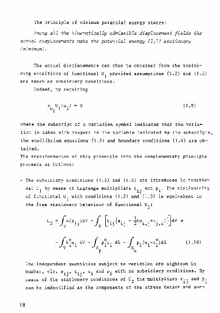
The principle of minimum porenti,,} energy state.s;

ilmong aU the Un<'"latic,aUy adm~:s8ible ,HspZacemen.t field" the

,,(:tl)cd dl:8p~aoementG make the potel1UaZ el1epg'Y (1.?) stO,tio)1.a,py

(m,:nimum) .

The actual displacements can thu~ h" obtained from th" minimi­

zing conofttons o[ [unctional VI provided assumptions (1.2) and (1.5)

are taken as ~uhgidiary conditions.

Indeed, by cequiring

o (1.9)

wh"re the subscript of a variation symbol indicates that the varia­

tion is taken with respect to the variable indicated by the subscripts,

til'" equilibrium equarions (1.3) and houndary conditions (1.4) are ob­

tained.

The tran!=lformatiol1, of thi.s principle into the complementary principle

proceeds as follows:

- The subs id iary cond i t ions (1.2) and (I. 5) ar~ introduced in functio­

nal U j by means of 1.agrange multipliers t ij and Pi' The st(>t~on(>dty

of functional Uj

with conditions (1.2) and (l.S) is equiv"lent to

the free .tationary hehaviour of functiOnal 02:

IB

1I2 c fW(e,,)dV - f It,,{e, - tCu, ,+u,)I]dV + Jv 1) J v L 1.) ~J ~d J,~

-lk~U. dv V 1 1

(I. lO)

The ind~pendent quant~tleg eUbject to variation dr~ eighteen i~

number, viz. e,., t", u. and p. with no subsidiary conditiOns. By ~J 1 J 1 1

meanS of the station~ry conditions of 1I2 the multipliers t ij and Pi

can be ind"ntificd <'IS the components of th" stress tensor and sur-

face streSS vector respectively. In subsequent chapters this identi­

fication procedu.e will be carried out in detail. It i~ omitted here

and U2

is immediately considered to be a functional with identified

multipliers. On taking variations with respect to the independent

quantities, Ilqs. (1.1) to (l.S) incl. are obtained. Fo.mubtion (1.10)

is sometimes named after Hu and Waahizu and can be rega.ded as a

generalization of the principle of minimum potential energy, sinc~,

if EqS. (1.2) and (1.5) are taken as subsidiary conditions, U2, is

reduced again to Ul •

The 8~cond step implies variation of the strains. The condition:

& U - 0 e .. 2

l.1

leads to the stress-strain relation:

"wee .. ) t .. _ lJ

1J ~ 1.1

According to (1.8) this means:

This relation can be inverted:

IntrOducing the complementary energy per unit volume;

(l.I!)

(I .12)

(1.13)

(1.14)

( I . 15)

this quantity can, by virtue of (1.14), be exp~essed ~n ~h~

stresses:

(1 . 16)

19

In our case this results in:

w c

I "2 Fijk~ti/H (1.17)

Under the a~sumpl;:iol1 (1.12) the strains can thos be diminate<J from

U2

:

-lw (t. ·ldV +jtcu .. +Il .. )t .. dV V c ~J V ~ • J J • ~ ~J

-f k~u. dV - r v ~ 1 J s

p~t.1- dS -1 P.(u.-u~ldS 1 1 S 1 1 1

(1.18)

p U

This functional is ~quivalent to that of the Hellinger-Reissner prin­

d p 1 e ~ The ill.d"p"nd~nt var iab 1 ~5 are t,., u. and Pl." 'J 1

- The third ste~~ which is due to Friedrich8~ implies partial inte-

gration of the proper term containing t ij in order to generat~ the

equilibrium equations (1.3):

U4

n -fw (t..)dv -fCt. ..... k~)u. dV .. V (: lJ V LJ,j L L

+J (p,-p~)IJ, S ~ , ~ dS + is p,u~ dS

~ ~ (I. 19)

p u

The number of independent variables can be reduced by requiring

equilibrium. Stress distribution consistent with equations (1.3)

" According to TONTI 2,2 in Reissner's original formulation compati­

bility of strains and displacements was assumed, as shown by the ab­

sence of the last term in (1,18), 50 that stationarity with reopect

to variations of tij yie~oeo the stress-st~ain re,ation, ,n O~T case

the stre~s~strain relations are assumed, so that variation of the

str~ss~s r€sults in the kinematical boundary conditiOns and, in­

dir~Ltly, in th~ strain-displacement relation~,

20

and (1.4) Ii.e s<,-id to be "statically admissible" Under these anump~

tions functiona1 U4

becomes, after inve~s~on of sign:

Us Dlw (t .. )dV -J Pi\l~ 0:15 V ~ q S

u

(1.20)

Thus it remains ~o vary t ij and Pi' Since Wc(t ij , is positive defi­

nite, another minimum prin~iple is obtained.

This p~incip1e of minimum potential energy states:

Among a~r statically admissibZe st~e88es the actuaZ stresses

make the complementary energy U. 20) stationary (mhdm1fft1).

Indeeo:!, by requiring:

6 U = 0 r:J •• 5

(1 .21 ) 1J

the strain-displacement relations (1.2) <'-nd kinematical constraints

(1.5) are obtained.

1.3 The relation of Herrmann's variational principle with other

variatiOnal principles.

The general t.linsformation scheme being presented in Section

1.2, it remains to place Herrmann's principle ip tnis scheme. We

sh~ll re~trict ourselves to only a simple beam problem 5i~ce this

will be sufficient for demonst~ating the argumentS.

Consider a slender, homogeneous, elastic beam of constant c~oss­

section (Fig.l .1).

This cross-section has an axis of symmetry. The x-axis coincides witn

the centroids, while the ~-a~is is pa~allel to the axi$ of symmetry

of the cross-seeton. Torsion-free bending in the x-z-plane has been

21

z

F-ig. 1.1 Beam, diapZaaements and ~oad8

realized by p~oper application of extern~l loads acting also in the

x-z-plane.

The beam has a length ~, a cross-sectiDnal area f, a modulus of

elalticity E aad a mom~nt of ine~tia X,

(1.22) .

integration heing taken over the croSs-5ection S of the beam, At the

end x=Q the displacernent~ are prescribed:

w' (0) ,,0 o

(1.23)

(1.24)

In Eq. (1.24) and in the foUo"'ing ones a prime denotes differ~nta­

tloo with respect to x, thus ( )' = d( l/dx.

The q"antiti~s M and Q (lre the bending moment and shear farce

of th~. cross-section, as shown in Fig. 1,2.

The beam is subjected to a distrihuted load qO(x) per unit

length, at the end xci to an end force P:, in the direction of a the z-axis ;.lrl0 00 external, moment MR."

22

"(j Q

. dx

Fig. 1.2 Positiv~ di~~~tio~s of Q and M

For this example the Herrmann functional 2.2 is:

and the subsidiary condition~ are:

H we 1:'equire:

we obtain as Euler equations:

M" " q

M - Elw" 0

(1.25)

(1.26)

(1.27)

(I .28)

(1.29)

(1.30)

23

and the natural boundary conditions'

M'U') - pO (I .31) z9.

w'(O) <to 0

(1.32)

Observation of the Herrmann [unctiOIlal (1.25) and its subsidi8ry

conditions (\.26) and (1.27) give. the impression that with the rele­

vant vdri~tional prinr,iple two streSs-displacement ~ystema are treated

in d differ~nt way:

o 0 - ter.ms - q wand - Pz

£ w(£), together with condition (1.26) would

indicat~ that the deflection is treated according to a potential

energy formulation. The pertinent stress Q(x) does not appear in the

formulation.

- terms - M2/2El; - M(O)4>° and condition (1.27) would indicate that o

the moment M is treated according to a (negative) complementary

energy formulation; th~ pertinent generalized displacement ¢(x),

i.e. the ~otation of the cross-section, is absent.

This hypothesis will he proved nOw. Th~ obserations imply that if we

wish to constr~et the Her.rnann formulation from a potential energy

formulation, both di~placements wand • should be preBent in thQ

starting formulation.

II consistent way to formulate such a functional with its subsi­

diary <;onditions is to Btart from II more gene.al bending theor.y where

the ~lop~ of the elastic ],ine and the rotations of cross-sections are

clearly "~parated, i.e. the bending th~ory accounting for shear de­

[ormation.

The relevant potential energy functional r~ads:

(\ ._33)

whare ( and yare the hending str~in and the shear strain re5pecti­

vely anJ G is the modulus of rigidity.

24

Kinemati~ally admissible strains and displacements must fulfil

the following requi~ements:

- the kinematical constraints

w(O) c wo o

o 4>(0) a ~o

- the ~train-di~placement relations:

y ~ ~ - w'

(1.34)

(I.35)

(1.36)

(1.37)

Returning to the theory of n~gligible shear (y*O), this formula­

tion becomes:

(1.38)

w~th subsidiary ~onditions: (1.34), (1.35), (1.36), whereas the

strain-displacement relation (1.37) becomes a kinematical constraint:

w' (1.39)

,his potential energy formulation now containing the rotation ¢,

forms the starting point for applying F~iedrichs'transfo~mation.

Since w is assumed to be treated according to the potential energy

formulation, the transformation is only applied to ~. This means that

the first ~tep • viz. introducing the subsidiary conditions in the

functional by means of Lagrange multipliers, is only taken for ~uh5i­

diary ~onditiQns containing ~,i.e.(1 .35),(1.36) and (1.39). As in

the pre~eding section, the procedure for identifying the multipliers

is omitted here and the functional wich identified multipli~rs is

2S

given Be once:

(1.40)

The second step implies variation with re~pect to thl ~trains

3no elimi.nillion of the ~trains, The requirement '\.U2

= 0 leads to:

M ~ Eh

and expressing K in M this gives for U2 :

=1£i-M2 o~ v .. ) = 1-- + M·t' - Q(~-w') - q w dx + o '- 21': I

(1.41 )

(1 .1,2)

The third step implies parcial integration such that the equili­

brium equation appears for the stress that we want to treat comple~

mentarily (M), If,on the other hand, we ~equire this equilibrium eo

be fulfilled the corresponding displacement ($) disappaer. from the

functional.

Partial integration of the term M~' gives:

U4 it [-M? - (M'+Q)¢ + QU' - q\,ldX ..

o lJn J

(1.43)

It we require M to be statically admissible,

M' + q (1.44)

26

( 1.45)

the following f~nctio~al is obtained:

(1.46)

Tbis is irtdeed the the same f~nctional as UH

(I.2$) wnile const~aints

(1.34) and (1.45) also ~orrespond with (1.26) and (1.27). Moreover,

the a~~umptiona (1.41) artd (1.44) are obtaineo. This result confirms

our hypothesis, and we may conclude that He~rma~n's principle can b~

derived by starting f~om a potential energy forrn~lation5 that e~able5

a dis~rimination between two st~ess-displacernent systems to be made.

When this condition is fulfilled, we apply Friedrich's transformatiOn

to o~e of these systems.

It should be remarked that owing to the term M'w' we cannot speak of

a mirtimum prirtcipl~. Moreove~, inversion of sign, as done in the last

step of Friedricna'trartsformatiort. is useless in this mixed formula­

tion.

Irt view of the a5s~mptions (1.41) and (1.44) the Euler equat~on

(1.29), being the stationary condition with respect to w, can be in­

terprete~ as the equilibrium of vertical forCeS;

o (1.47)

wnile equation (1.30), being the st~ti,o~~ry 1;ondition with respect

to M, cart be inte~preted as the strain-displacement relation;

K l1li W" (1.48)

Tne~e re~ults are also consistent with a potential energy approaen

and a complemerttary energy app~oach ~espectively.

27

CHAPTER 2

Extension or Herrmann's variational principle for the case of geometrically

non·linear bending of beams

2.1 Introduction

in thi~ cha.pCer H"rrmann· s variational pr inc iple will i)e extended

to geometrically non~lin£Qr bending for the c~se of a hearn. The pri­

mary aim is to apply and explore the approach and prove its validity

in a mathematically simple situation. After establishing this form\l­

lation it can be used 3S an an~logue for deriving the ext~nd~d varia­

tional principle of n;,rnnann for the case of the geometrically nOn­

lim!JI beI\diI\g of plates.

"'ben deriving tbe desi.l;ed f.ormulation, the same procedure will be

followed as in tlle linear case. The beam itself, however, will be

treated as a special case of the general large-dbplJcement theory of

elasticitYt because it 1~ felt ellac specializ3t~on from a general

[heory forms J soundon basis than gene~ali,"s.tion of s. more restricted

theory. In particular, the symmetric Piola-Kirchhoff stress tensor

s .. will bE used. This notion of stress has been flJrtller developed by 1J :1 I

KAPPUS • AppeIldix A gives a SI.ImJ1I(H·Y of the relevant eq\lstions.

In Section 2.2 we will develop the required starting potential

energy formulation that takas iIlto account traIlsverse shear defor-

rnation.

In Section 2.3 this forrnuhtloIl will be used to oedve the govern­

ing differential equations and Ilatural boundary conditions.

28

Restricting ourselves to the ca.e of neslisible .hear deformation,

the formulation will be u.ed tD derive the extended p~in~iple of

Herrmann (Section 2.4). The pertinent Eu~er equations will be com­

pared with the gove.ning differential equations to prove the correct­

ness of this formulation.

2.2 Potential energy formulation for $eometrically non-linear hending

of beams, including the effect of transverse shear deformation

For the case ot neglected shear detormation the potential ene~gy

formuLation is given by KAPPUS 2.1

The procedure outlined in Chapter I, however, req~ires a starting

potential energy formulation which enables ~s to distinguish two

stress-displacement systems, one remaining ~nchanged, the other to be

transformed according to the general transformation scheme. To that

end, a pot~ntial energy formulation. initially taking into accOunt

~hear deformation, i~ needed. This formulation will be developed now.

Consider the same beam as treated in Section 1.3. Now the loads

are of such magnitude that it is nO longer justifiable to use the re~

lations of the linear theory of elasticity. Instead, the large-dis­

pla~~mertt theory of ~lasticity must b~ ~s~d (see e.g. FUNG 2.2). The

governing equations are summarized in Appendix A. The description we

wish to follow 1. Lasrangian, i.e. with reference to material coordi­

nates. We choos~ a fixed rectangular coordinate system ~,y,~, such

that the a~i~ of the unloaded beam coincides with the x-axi~. Material

points of the beam are identified by their ~oordinates X,Y,Z, relati~

v~ly to the x,Y,z sy~t~~, in this initial position. The value~ (X,Y,Z)

remain fixed to the material points when the beam deforms. The new

position of point (x,Y,Z) is:

x = X + u* y = y + v, z = Z + W (2.1 )

where u,v,w represent the displacement. In the Lagrangian descrip­

tiDn th~ symmetri~ Piola-Kirchhoff stress tensor will be used.

In addition to the boundary conditions pre.ented in Section 1.3,

at the end XeD a displacement uO in the x-directiOn is prescribed, o

29

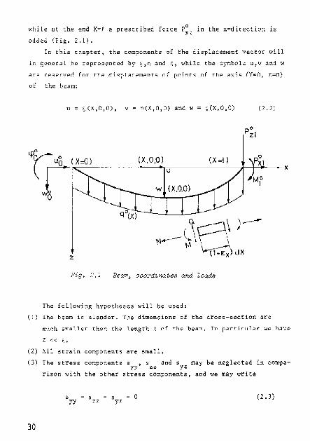
while at the end X-' a preseribed force P:A

in the x-direction is

,Hided (Fig. 2,1).

In this chapter, the components of the displac~m.nt vector will

1[1 generdl be repreB~nted by ;,n and 1:, while the "ymbols u,v and w

.are reserved for th-e digplacement5 of I?oints of the axis (Y'IIIlO.,. 7.:=0)

of the l>8~m:

u = s(X,a,O), v - ~(X,a,O) and w ~(X.().O) (2,2)

(X,D,O) ------------~~-r~--~x

z

Pig. ,~.1

The following hypntl1eses will he used:

(I) The heam is slender + Tl1e di.men,sioTIs of the C.f05S-S12:LtioIl ar~

ro,\~h 5Il1al.l~r tlH'n the length ,~ of the- beam. In particular we have

(2) All strain components are small.

(3) The streSs components 8 ." and" mal' be neglBcted in compa-yy zz Y7-

30

risOn with the other stress components, and we ~ay write

s =, yy 'zz 8 yz

o (2.3)

(4) Cross-sections whi~h were p8rp~ndicular to the a~is of the beam

before bending, remain plan~ an~ suffer no deformation in their

planes.

With theBe assumptions a potential energy formulation will be derived.

Denoting the rotation of a cross-section by ¢(X). the relation~ be­

tween the displacements become (Fig, 2.2):

;; = u - Z 8iM

n = 0

- w - Z(I-cos¢)

..f.x lrf __ ---:'~~~ .. _.,t!._-~: ... --.~~:~:---{-=-,.-:::;-~-)d X ~z

z

B

-. ,.-.. --.-;:;----=-1

t----~~

Fig. 2.2 Re~ation$ be~@en displacements

(2.4)

(2.S)

(2.6)

w

aw dX ax

It must be re~arked, however, that (2.4) and (2,6) are inconsis­

tent as regards the accuracies of the individual ~ontribution5 to ehe

displacements ( and ~. Since the assumption that the length of AB is

31

lhe sam~ in the unloaded as well .s in the loaded configuration im­

plies an inaccaracy~ it is superfluous to tak~ account of t11e contri­

hution DE t as accurately ~s given by sin$ and cost respectively. it \ 3) wOI.th\ be more cond~t.nt to replace [or instance Z ~inq, hy Z(¢- -g1' .

Notwithstanding thi:!i t the trigonometric cxp~essiona are. retai:r'H.'d in

the formulations to fad litate interpretation of derived "e"pre~dons.

According tu the stress hypothasis (2.3) the specific strain

en~rgy ~an he written aij[

+ 2 s ~ Xl' xy

+ 2 8 e ) X2 XZ

and U8ing Hooke's lay: .. we have.

w - -21

(Ee" )oe

+ 4 Ge? + 4 Ge' ) xy Xl.

(2.7)

(2.8)

lis to the strains, we diffe,entiate between strains at pOints (Y-O,

Z~O) or the axis of the beam and strains at other points, The l.Hter

will be Overh~rred. Hor~ovRr, for the shear components we introduce

the quantities = 2 e (y = 2e ) and y = zev

•• (Yxz = 2e ) xy "y xy "y X? M. xz

Tbe non-linear strain-displac.ement re.ltitiOns art!:

e xx

'txy

y xz

'r. + oX

~ C + <)y

+ [O~)' )~ 3( - + rx dX

+(~~Y+(~~YJ ill; 3~ 3n + ~~ 3Y ~~~ JX n oX 3Y

Introduction of Eqs.(2.4), (2.5) and (2,6) gives:

32

e xx

(2.9)

(2, \ 0)

C2.\\)

(2.12)

o (2.13)

(2.14)

For sm~ll str~ins. the first expression can be 5impliti~d along the

following lines.

If w", denote the angle of shear ln

ment aX the new

is rotated aver au angle

length ds, e>lpre~~ed in

ds = (1+<; )dX x

According to (2,12) we have:

e KX

¢+i¥ "z

u,.w and

the x-z-plane by ~)X2; ,

and from fig. 2.2 we

¢ is:

For small shear angles, ~ <~ I,Eq.(2. 15) can be written as: xz

(I+£X) - {(I+u')cos¢ + ~'5in¢

+ ~ {w'cos¢ - (1+~')5in4f xz

C~mbin~tiQn of (2,17) and (2.14) give,:

{(I+u')co5¢ + w'sin~l

an ele-

see that

(2. 15)

(,.16)

(2.18)

In view of (2.16) and (2,18) relation (2. 12) c~n be written as:

exx (2.19)

(2.10)

33

With (2.8), (2.13) 3nd (2,20) th~ ~lAstie strain energy of the whole

boam becomes;

w = 1 ~f [.!. E(e -Z,')2 + -21

G Yxz2fd5 dX X=O S '2 xx

Thus, fo>:" a bell'" witl' boundary conditiOIls as shown i.n Fig. 2.1, After

i,lt.,gration over che cro~~-section S of the beam, the potential .mer­

gy f\l\\ctio~al h",come~:

(2.21 )

where a hending strain ~ is intToduced. Strictly speaking, this ben-

ding strain is not the curvAture of the beam; only if .x

this bending "train equ~l the curvature.

The subsidiary conditions are~

- I;he strain-displacement relations;

e xx

¢ ,

I)' + 1 , "-'2"

y ~ w'cos¢ - (I+u')sin~ xZ

- the Hnematical c.onstraints:

\1(0) 0

u D

w(o) ~

0 w

0

¢(Q) ¢~

34

0, dOes

(2.16)

(2.22)

(2.14)

(2.23)

(2.24)

(2.25)

If shear deformation can be neglected (Yx~~O) , the strain-displace~

~ent relatiOn (2.14) becomes a kinematical constraint:

arctg (2.26)

Again, this relation is inconsistent as regards acc~racy but will b~

retained because it facilitates interpretation of relations to be

derived

2.3 Forces and moment of the cross-section, and heam equations

Prior to the d~rivation of the extended formulation of Herrmann's

variational principle some auxiliary equations will be derived. This

is necessary since an important step in the procedure to be followed

is the introduction of some subsidiary conditions into the potential

energy functional with the aid of Lagrange mu"tipliers. These multi­

pliers are to be identified with physical quantities and this is im­

possible without knowledge of the governing beam equations. Therefore,

these equations will be derived here. Moreover, they can be compared

with the Euler equations of the Herrmann formulation to be obtained,

thus providing ~ proof of the corre~tnees of the latter.

E>:pressiol'ls for forces and moment of the cross-section consistent

with our potential energy formulation (2.21) Can be obtained by com­

paring its variatiol'l with the virtual work equation, expr~ssed in

quantities of the cross-section:

(2.n)

ln this expre5sion O~ and 6yxz

are variations of true deformd~ions.

The true exial strain, however, i~ ~x' So the virtual work, performed

35

by the forces and mottl,;,nt of the cross-section and the ext .. rnal load;;,

j,$ :

oW . vlrt

(2.28)

Ih. relation between [ and e is (see A 9) x xx

I + [ =.J I + 2e x xx (7..29)

and the relation hetween tht!:ir vilriationf! is:

(2.)0)

III 'Il ew "f tiH' assumption of small strains. EX could be neglect .. d

wbert compared with I. The. term (1+ .. ,,) is retained as a label, how­

ever, in order to facilitate interpret~Cation, see. e.g.(2.44).

Co~p8rinB (2.27) and (2.28) gives, In view of (2.30), the following

relationg~

N RF(I+[ )e " xx

(2.31 )

M Eh (2.32)

Q = GF Yxz (2.3J)

The equilibrium equations and dynamic bo~ndary conditions are

obtained as the Euler equations a,td natural bounda,y <;:.onditions of

Eqs.(2.21) to (2.2:;) inel,

(2.34)

36

With

Ii""xx 0 {(l+u'>ou' + w'liw' I

(2.37)

it follows from liUMO:

(2.38)

{EF~ 101' + GFy COS$}' + qO = 0 xX x,Z

(2.39)

(2.40)

(2.41 )

(2.42)

(2.43)

That these are the relevant equilibrium equations can be shown by ob­

servin~ that (I+u') artd 101' of EQs.(2.38), (2.39), (2.41) artd (2.42)

are rehted to the art~le (co) between the deformed axis of the beam

and the X-~Xi5 (l'ig. 2.3) as follows:

sino. 101' J+u' w'

1+[ co.ea i+7" tga I+u'

(;2.44) X J(

lntroducirtg (2.34),{2.3l),{2,32),{2.33) and (2.44) into the Eqs.

(2.38) to (2.43) incl. gives:

/NCOSOl - Qsin<P\' o (2.45)

/Nsina + Qcos~\' + qO ~ 0 (2.46)

37

(2.47)

(2.48)

(2.49)

1'01, = M~ (2.50)

Th"t these .He the proper equations follows from ,'ig. 2.3:

N~. -._", •.•. , ..... , .. ----~ X

tv'!

~x N+N'dX

Q~Q 'dX

z

Fo~ce{; a,atirtg on an dement elx

If shear deform.tio~ ~an he negl~ttQd (o=*), the equilibrium

equation (2.47) h~eomes:

1'01' = - (I+',,)Q (2.51 )

Moreover, in that case the relation hetween the b~ndiDg strain K and

t.h~. displacements u en w becom.-:s by introduction of (2.26) in (2.22):

38

(t+UI)Wil ....... w'u"

( 1 +u ' ):' + w' 2 (2.~2)

2.4 Derivatiort of Herrm~nn's variatiortal yrinciple in ~ase of geometri­

cally non-linear bendinA of beams

The preparatory work being done in the preceding sections. the

derivation of Herrmann's variational principle exten4ed to ~eometri­

cally non-linear bending will now be ta~en in hand.

The potential energy functional (2.21) together with subsidiary

conditions (2.14). (2.16) and (2.22) to (2.25) inc.l., form the ~tart­

ing point for applying the precedure outlined in Chapter l. Since we

confine ourselves to the case of negligible she~r deformation (YxzcO),

condition (2.14) must be ~eplaced by (2.26).

According to the procedu~e, only the (M,t) ~ystem will be sub­

jected to the trans£or~ation into a complementary £or~ulation. ln

consequence, only sub~idiary conditions containin~ ~ will be b.ougnt

i~to the framework of the £unct~Dn~l ~y means of Lagrange mUltipliers

in order to introduce the genera,ized force consistent with ¢, viz.M,

into the functional.

Ihis implie~ that the non-linea~ condition (2,16) remains one of

the SUbsidiary condition~ irt th~ formUlation to be obtained and does

not co~plicate the transformation.

The sta~ting formulation is:

where AI(X), '2(X) and '3 a~e multipliero•

The remaining subsidiary conditions are'

e x:':

u t +! u' 2 • l Wi 2 2

u(O) o u o

w(O) CI WO o

(2.53)

(2.54)

(2.55)

(2.56)

39

The independent quantities subject to variation in functional (2.51)

.are Seven in number; u, lo):i ¢ II k;' and the: multi:pliers }'l ~ )'2 and \3'

In thi~ ca~e, tilis formulation is equivalent to the original one.

Ih~ re4uirement DE a stationary heha.viour with respect to the multi­

plier. would give the origin~l subsidiary conditions:

,~ . (2.5:1)

,~ -arctg w'

(2.58) ~

:(0) ,p 0

0 (2.59)

Our 1~)t~'[u:io~L ib~ huwever, to rt'cinsfot"m rhi;s forIT'luldt.ion. Contrary

to Cl1.3pter I, the identific~tion of the multipliers will be given.

Sta~lonary behaviour of U1 with re~pect to • and ¢ gives:

'I(X)

- A I

(2.60)

(2.62)

(2.63)

A comparison of (2.60) with (2.32), together with (2.61), gives:

)

I M (2.64)

M(O) (2.65)

introduction of (2.64) into (2.63) and comparing the recsult with U.51)

40

(2.66)

This means that by means of the Lagrange multipliers the shear force

Q and the moment M of the cross-section are introduced into the

functional:

(2.67)

The second step implied the requirement of a stationary behavio~r

with respect to K. Requiring 6.U 2 = 0 gives:

MEl" (2.68)

~his res~lt is use~ to eliminate the de£ormation " from (2.67) by

mean.!;! of ~

(2.69)

Step three implied partial integration to gen€Ldte an equilib~iurn

eql,l~tion'

If we require the moments to be in equilibrium: (2.70)

(2.71)

Me£) (Z.72)

41

the exten~ion of H~rrmannl~ variational princlple to geometrica1ly

non-linear \lending f.or the case of a slender be!'1ll is obt,,~ned:

u = r \!.. F:F~ 2 H J X~O \2 xx

M2 "I' 0 l - ffi- M' arctg \+1,1' - q w dX +

(2.73)

The ~1,1l)s~di.~ry conoitions are U.54), (2.55), (2 •. ')6) and (2.72). The

linear formulation (1.2.5), (1.26) and (1.27) can be obtained as a

special caSe \ly taking 1,1'=0 and w'« I.

The principle states:

Among aU d{~p[w:>"m"n.t8 1. and IJ IJll·/.:,:.h $a./.i.r;f:4 "the pre!;ora'ed geom,,­

trlcJa/ VoundaI'!j oon,HMona, and amOng aU moments M whioh !;QUaf!!

"the, pl'<;w!r'':b"d (Zyn<1J1l-i(' boundal'Y ('onrlitl>Jnf3, I;;h(, Q('tuat dicpZao"m"nt$

m1d lIIolllrmt mak,! I;;hG Her"f'mann fU"l('I;;,;onat flta.i:ionary.

It i~ noteworthy that when fully transforming the potenti.al

energy formulation of ~ geometrically non-linear problem into iC$

compl,:,mcI~tary formulatioI"l, a major problem is that after requiring

equilibrium the displac~meI"lt" do not disapp~ar from the formulation,

but products of stresses and displa~ement derivates remain. Both

ZUBOV 2.3 and KOlTER 2.4 hava taken significsnt steps towards eX­

pre~dng the complementary energy functional solely in stresses. In

our partial, transf"rm"tion of the poteutial energy form1,11ation intO

the mixed He~~mann formulation this problem does not "ppe,,~; "'heu

requiring the equilibrium equation (2.7]) to be fulfilled, the re­

SUlting fun~ti"nal (2.73) beCOmes fUlly independent of the relevant

displ,,~ement ¢:

2.5 Correctness of the formulation

In this section it will be proved that the stationary principle

presented in Section 2.4 is indeed eq1,1ivalent to the governing set

of equations as derived in Section 2.3.

42

The governing equations are:

- the strain-displacement relations (2.16) and (2.52)

- the equilibriu~ ~qoations (Z.45), (2.46) and (2.51) with, in view

of the negl~cted shear deformation, ~c~,

- th~ ~onstitutive equations (2.31) and (2.32),

- the kinematic constraints (Z.23), (2.24) and (2.25)

- the dYnami~ constraints (2.48), (2.49) and (2.50).

In the Herrmann principle, equations (2.16), (2.51), (2.31),(2.32)

(2.23), (2.24) and (2.50) have already been assumed. It remains to

prove that tbe stationary conditions of the Herrmann functional (2.73)

are equivalent to (2.52),(2.45),(2.46),(2.25),(2.48) and (2.49).

Requiring DUH g 0 with respect to variations of u, wand M res­

pectivelYt gives as ~uler equdtiort5~

and as natural boundary condition:

{arctg 1:~1 } 0 4>0 o

o

M' (I+u'_) _}'+ qO " 0 (2.75)

(I+o'}2 + w·?

(2.76)

(2.77)

(2,78)

(2.79)

43

We perform the [allowing operations:

- the strain .xx is introduced by using assumption (2.16),

- the axial force N 15 introduced by using consitutive equation

(2 • .11). It should be remembered that (1+,) is relac"d to u and '"

hy:

(2.80)

~ the sh"n force Q i, introduced by using assumption (2.51).

- according to (2.58) it is ju~tifiable to introduce ao Rog1e • as

defined by (2.5H).

The,,, ()pH'~ t j on~ performed i it turnS out tlwt:

- Eut~"(' equation (2.74 ) 15 equivalent to the equation expresl:iing the

equilih[,"lurn of forces in til,;: x-direction (2.45) •

Eut"r equation (2.75) is equivalent to the .. qua tion expressing the

eql.d 1 i.br il,lffi of forces in the z-direction (2.46) •

- Since the con~titutive equation (2.32) was assumed, the Euler equa­

lion (2.76) is eq\lival",nt to the strain-displacement relation (;1.52)

or. expressed in @, the 5train-di$placement re"atian K~¢'.

- 1'l,lturnl l!oundHY 8ondition (2.77) is equivalent to the dynamic

boundary condition (2.48),

- Natural houndary condition (2.78) i.s eq\livalent to thE: dynam\c

houndary conditiOn (2.49).

- N,Hu!",," ['''llUd.uy c.ondition (2.79) is Eqlli"ale~t to the kinematic

constr8int (2.2.).

Since this completes the Get of go"er~in~ equations. the Herrmann

formulation as obtained in Section 2.4 is correct.

F:quation5 (1.29) to (1.32) inci. can be obtained as a spedal

case of (2.74) to (2.79) incl. by assuming u'=O and w' « I.

44

CHAPTER 3

Some procedures for obtaining frnite element models

3.1 rntrodu~tion

In the lin~ar dom~in. th~ finite element method b~sed on

Herrmann's variational principle offered an attractive solution to

problem~ encountered when analyzing plate bending by means of a

finite-element method based on the principle of minimum potential

energy. Since in the geometrically nOn-lin~ar domain the same pro­

bl~ms ere encountered, it wa~ felt that by means of an extension of

Herrmann's vari~tional principle to this domain these dLfficulties

could also be ev~ded. Th~ ultimate aim being the analysis of th~

geometrically non-linear bending of plates, it was decided to ex­

plore the extension of Herrmann'. principle for the mathematicallY

simpler case of a slender beam, loaded in a plane and deforming in

th~ same plane.

In the p~eceding chapter the pertin~nt functional together with

its subsidiary conditiOns has been derived. Thus, in the present

chapter, attention will be given to some procedures for obtaining

finite-element mod~ls with the ext~nd~d Herrmann formulation.

Notwithstanding the fac:t that the considerations of this chapter

are still related to the b~am problero, they hav~ a much wider meaning

and can be generali~ed to the probl€m of the benoiog of plat~s.

Section 3.2 gives a short des~ription of the finite-~l~ment method,

convergenc:e crit~ria and' the requirements to be mad~ on the approxi­

mating functions.

Section 3.3 gives a summary of existinS procedures for formula­

ting finite-element models as used in the analysis of the geometri-

45

cally nDn-l inc<l1; bending of beams and plates by means of the prin­

ciple of st~tionary potential energy.

In Section 3.4 it will be exemplified for the beam tlH't 8n<>10-

gallS procedures can be used wh~n the anaiYBis is bBS~d on Herrmann's

ptinciple. in Sec.tion 3.5 a finite-element model for beam problems

h~sed on one of these p~ocedures will be pre.ented, while Seccion

l.h give5 some numerical relultY. AnOther procedure will be applied

in connecLion with plate hending in thl next chapters.

3T2 The: finite-element method and COI"lVet"gence criteria

lhe finite-element method which is based on stationary conditions

of a fUl1~tional can h~ reg8rded 8S 3 particular form of the Ritz

mrtlwd 3.1 for obt~lnin8 approximatl solutions of the Euler equations

o( thut functional. The characteristic featura is that the approxi­

mating functions are piecewise defined on the domain.

Thre~ st<l!?;e. (:'m b" distinguished in tile method:

(a) Sele..-:tl0f\ of ,".e finite numbet" of points in t.h-e domain of the

[unction5, to wl,i~!, riiscret~ valu~s of these functions (and

possibly o[ some of their derivatloIls) will be a5si~n"d. Thes"

points are call"d nodat points, or simply nod"".

(b) Subdivision of tile dorn.~in into subdomains: the. finite. elements.

hie reSIl>:O the actu<ll domain a .• an assemblage of finite elements,

connected Lo~"ther appropriatelY at nodes an their boundari~Y.

(c) The functiOn iE apl'rO}(imated l.oCo.Uy within each finite element

by continuOUS funclions which are uniquely defined in tarms of

the values of lhe functions (and possibly of sOme deriv8livcs)

at ttle nodes of tIle elementl

An important Osp.cl of the finite-elam.nt method is that an alQ­

meet can b0 regarded as disjoint from the structur~ to be analyzed

when formulating its contribution to the whole structur~, sinca the

local approximating Eunction~ are expres~ed solely in values at the

nodes of that elem",nt. This implie.s tl"~t for each element a s\dtahle

.ystem of independent <coordinates can be chosen: tile loc,_] coordinate

46

system, For the whole structure, a common coordinate system must oe

chQsen; the global coordinate system. bn advantage of the local coor­

dinate system is that it facilitates expressing the local approxima­

ting function. When assembling the elements, a coordinate transforma­

tion may be necessary. One example is a three-dimensional framework

composed of beams whose local hehaviour ~an be described by one-dimen­

sional functions.

The choice of the shape of the element, the number of its nodes

and its location with respect to these nodes is determined by the

desired applicability of the element, the selection of the approxima­

ting {unctions within the element, and the continuity requirements

of the approximating functions over the whole domain,

For instance, when approximating displacement f~nction~ in case

of plane stresS, ~omplicated structural shepes can better be des­

cribed by means of triangular elements than by rectangular elements.

when deal ins with a cho~en linear displacement distribution within

each element it is only possible to obtain continuity of the dis­

plac~ent~ acro~~ element boundaries, if each element contains three

nodes, each coinciding with an angular point of the triangle.

The choice of the approximating fUnction~ within each element is

restri~ted by the requirements of the variational principle and

sho~ld meet the convergence criteria.

If the variational principle concerned ,s a minimum principle and

the functions meet the requirement~ of that principle, then the con­

vergence criteria are those of the Rit. method. For instance, in case

of two- or three-dimensional elasticity, the principle of minimum po­

tential energy requires the displacement~ to be continuous over the

whole domain, while within each element the strains should have bounded

and continuo~s first derivatives. According to the convergence criteria

of the Rit~ method, however, this i5 not a suffi~ient condition. To ob­

ta~n convergence, it i. necessary that the displacement should fulfil

the ~o-cal1ed completeness criterion, which in this case means that the

47

scrain~ should be ahle to assume arbitrary constant values within each

element.

U the re.levant variation~l principle is not a minimum principle,

as is the case with H~rrm~ntl's v~r1ational principle, toen the cOn­

vergence ~riteria cannot b. derived in the same way ~s tho~e of the

Ritz method. However t ticcording to OLIVEIRA 3 1 2, even in tbi:!;l ca6e

and in cas" o[ a minimum principle with incomplete continuity of

the fields between the element.~. it proved to be possibl,e to formu­

late convergence cd.ted ~, Th1,l5, complete cotltinui ty. al though a J:e­

quirement of the principle, is not neceRsary for convergence.

According to Oliveira, for the mixed Herrmann formlliat'lon if

she,H deformation is n"glected and if we remain in the domain of tll",

linear tlleory of elasticity, convergence wi).1 be obtain"d if:

- the displacements at" continuous ac);oss the dement boundaries and

tIle bending moments re.pect the equilibrium "quartans on such boun­

daries; thie is a requiramQnt of the variational principle;

- the compl"reness condition is respe~ted for the displacements as

well a" the bending moments, which ~n this caSe means that both

the strains and th" moments can assume arbitrary constant values

within each element.

since a convergenCe theory for th", approximate solutio\l of geo­

metric~lly non-linear problems is lacking it is felt that the best

we tan do to cr~ate condition. for conv~rgance, is to reopect th~

afor"mentionad critc~ia of the linear theory.

3.3 Some alternative finite-elemant procedures as u~ed ~n th~ statio­

nary potential en~r~approach

For the finite-element anal1sis of the eeometrically non-linear

bel1ding of beam" and plate5 by me~n~ of che principle of stationary

potential energy, some alternative procedures have emerg~d (see ""g.

Refe~cnc~s ],3, 3.4, 3.5 and 3.6).

48

The b~sic differencee are charaterized by:

- the local coordinate sy~tem that can be chosen for each individual

elemenL.

- the degree of non-linearity inco~po~atect in the ctescription of th~

individual element ~e18tive to its chosen local coordi~ate ~y~tem.

To typify the degree of ~on-linearity, the followins qualitative

ranges of displacement, as used in plate theories but also applicable

to beams, will b~ distinguished:

- finite d~fl~ctions, i,e. th~ displacements in th~ plan~ of the plate

and their first derivatives a~e of the same order of magnitude as in

linear theories. The displacements perpendicular to the plane of the

plate (th~ defl~ction) and their first derivate5 roay be larger. An

example of a theory cOn$truct~d On thes~ assumptions is offered by

the von Karman plate bencting theo~y 3,7;

- large displacements, i.e. neither the in-plane ctisplacements no~

the cteflections remain in the ctomain or linea~ theories.

The loc~l coordinate system can either be fixed in the initial,

unloa~ect position of the element or mov~ with th~ ~lem~nt.

Considey a beam element bounded by nodes I ~nd 2 lying in ~ p1ane

and deforming in the same plan~ (Fig, 3,1), To d~scribe the geometry

of the ~hol~ struetur~, W~ establish a fi~~d Cart~sian global coordi­

nate 5yst~m x,z. In thie system the coordinateS of a material point

of the undeformed structure are X,Z and it. displacements u and w. X

and Z are ~al1ed material coordinate~, In addition~ we introduce for

each element a f~xed Cartesian local ~oordinate ~ystern. x' .z~, In

this system the material coordinate is x*~ whereas ZM=O. Since the

position of this local

49

Fig. ".1

* :;:; z

E'1E'mE'nt

--------------------~ x

Globa? aoordl:natee

InUiat taoal- aoardinates

coordinate syG(",m is det"rminell by the ~nlO,jlded, j,nitial poddon of

the Qlam~~t. we call it th~ i~itial local coordinate system. The

tran"formatio~ betwae~ global coo~dinates ,jlnd initial local coordi­

nates is <:ornpletely d<"!t"rrnin~d by the initi,jl~ geQmetry of the struc­

tu<e and independent of the global displacements of node~ of the el,,-

ment.

Such fixed local frames of refe~ence have ~p to now only bee~

used within the range of finite deflections fOJ" the whole structure.

This implies that the finite oeflection belH!viour must he incorpo­

rat"d in th" model of the indivio\)al element. U~ing the von Karman

plat;: be~ding theory, this approach ",as applied hy BREll11IA and

CONNOR 3.3 and by lll':RCAN 8..,Q GWUGH 3.4

In this ca$e the coordinate sy5te~ ~OVe~ ~ith the deforming ele­

ment "'hen the str\)ct.l.lre deforms, bllt retai~s its initial metric (Fig.

so

3.2). We call this system the displaced local coordinat@ system. The

origin of the moving coordinate system is attached to a particular

node of the element, while its orientation i~ deter~ined by the di~­

plac~ment~ of ~ome other nodes of this element. So, in this CRse,

the tTansfoT~tion between d~5placed local coordinates and fixed

global coordinates is determined by the initial position of the ele­

ment as well as by displacements of nodeS .

z • z

~o

L-__________________ ~ __________ ~ __ ~x

G~obal ¢oo~dinate8

Initia~ ~ocal coordinates

Disp~aoed ~ocaZ coordinates x,z

Glohal displaoements U,w

Loaat displacements

Fi~. 3.2 Coordinate and displaaement nomenc~ature

We can envisage the overall effect of the deformation as consis­

ting of two parts:

(I) the element is translated and rotated as a rigid body together

with the moving coodinate system

(2) the element deforms relatively to the moving ~ooTdinate system.

51

The displaced local coordinates should not be confuse<:l with the

bo-c~lled convected coordinates (see e.g. FUNG 3.7 p.92). Wh~n wo~­king with convected coordinate~, a distorted coordinate system is

chosen so that [Dr all material points the coordinates in the deform­

formed configuration with respect to this system have the same nume~

ricdl values dR their coordinates In the initial coordinate ~ysteffi

wllen IIndeformed.Tn our case, however, tlle displaced system is unde­

formed, while only the IIlat.erial point attached to the origin of the

displaced l"c .. ~l coord in8 te system preserves the same coordinates re­

latively to that system as in tlle irdtial local COOI"dinBte 6ystem.

When using this moving systew, tbe behaviour of the element

relative to this systE:,rt can either be described by tbe laI"ge-dis­

placeme~t theory, the finite-deflection theory or the sm~ll-di5-

plac€me~t theory. By ~irninishi,ng the element dil'llensiotls, it becomes

justHiablc to lise tlle fi.nite-defle~.ti.on cheory or the small-dis­

placement theory sllccessi,ve1y for descI"ihing the elel'llent behaviour,

a1 thOllgh the glob.,] d j spla~ements may be large. The great ,,(lvantage

of this procedure is the simplification of the description of the

finite element itoelf. If element dimensions are sufficiently small,

known ~lement mo~els of the linear theory can he used, while all non­

litle<lrities "r~ embodi",d in the transformation from the displaced

local to the fixed global coordinate system.

Ihis approach has been used by various authors,

BESSRLING 3.0 analyzed plane beam structures. He obtJ.ined the

discrete non-linear equations for the individual QIQm0tlt hy using a

di.screte vhtuB1 \Jork equacion of th" linear thQory and by expr~.5sing

the generali'ed ~lemenc stI"sins (i,e. a nodal displacement and nodal

rotations relative Co the displaced locel coordinate system) directly

in the glObal nodal point displacements of the element. Then the ele­

ments are aSBembled in thE: usual way to obtaj,);l the l1on-lineaI" equa­

tions for the whole structure.

52

MURRAY and WILSON 3.6 analyzed large-displacement p<ate bending.

They formulated the element stiffness matrix by using the linear

plate theo~y and expressing the potential energy in the small dis­

pLa~ements rela~ive to th~ displaced lo~al coordinate system. This

stiffness mat~ix is used in ~ombination with the non-linea~ ~elations

betw~en displaced local and global displacements.

3.4 Alte~native finite-element procedures for the Herrmenn formula­

ti.on

In the pre~eding sections a brief de$~ription of the finite-ele­

ment method and some alternative procedures for formulating finite­

element model~, as used in ~onnection with the p~inciple of statio­

nary potentisl energy, was presented.

Now it will be exemplified for the beam that toe same pro~edures

can be used when basing the finite-element method on Herrmann's prin-

~iple. For simplicity, we do not die~insui~h bet~~en the initial

lo~al and the global coordinate systems. rhe coordinates of the fixed

Cartesian system are x,z. Again, a Lagrangian description i~ ~hosen.

The material coordinates o£ pointe of the axis of the beam are X.

nifferentiation with respect to X ie denoted by a prime: d( )!dX =

( )'. The contribution of the k-th element to the functional of the

Whole structure is:

~k = r [-21 EFe 2 J ](=0 xx

(3.1)

where ~k is the initial lenSth of the k-th element. The subsidiary

condition is:

e xx

The functional of the Whole stru~ture is:

(3.2)

(3.3)

S3

where UH ext represents the contri.b1,lt i on of pr,,~cribed loa.ds and ro­

t<lt.i.ons according to the conventions of the Herrmann formulation.

When 3ssemblins th~ elements, continuity of t\1e di8placement~ and

equilihrium of the bending moments ffi1,lSt be respected. Now, " s1,lit­

ahle local coordin~te systeem can be chosen [or each element.

(a) ~_fb~£~_~~£~!_£~~~~i~~E~_~Z~£~~ may be suitable if the deflec­

tions of the whole str1,lctl,1r~ remain finite. The 3ss1,lmptions are:

u'«1 and (w')~ = ~1,l'), b1,lt at the same time w' must remain sO

amall that the approximation arccg w'· w' is justifiable. Then

(l,]) and (3.2) hecome:

~k

1 [.!... J':Fe < int x=o :2 I xx

e Xx

- ~ - H'w']dX 2EI

(3.5)

The only remaining nOll-line8dty to be incorporated in the model

of the finit.e element iti;elf h thoe influence of deflection on

the stretching of tne B}{i~ of the beam as given by (3.5). This

approach ~ill be used for the analysis of plate bending in the

next chapters.

(b) !~~_2i~El~£~£_1£~~1_~££~~~~~~~_~Z!~!~ x,z .may be so ~hosen that

the origin is connected to the end K~O (node I) of the beam,

while the end X=lk, (node 2) :remains on the ;-axis. The :rotation

t(X) of a croas-sQction can be considered eo have been obtained

54

in two steps:

- a "ontribution ~ due to the rigid body rotation of the element,

and

- a contribution ~(X) due to a rotation relative to the dis~

plac<i!d local "oordinatQ systel1l:

(3.6)

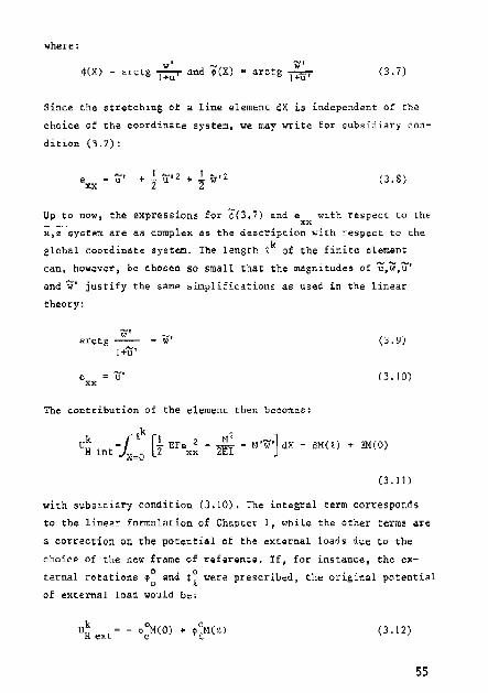
where:

~ClO w' W'.

arCcg ~ and ~(X) • arctg 1+%' (3.7)

Since the stretching of a line element ~x is £ndependent of the

~hoice of the coordinate system, we may write for s~beidia~y ~on­

dition 0.2):

(j.S)

Up to now, the expressions for ~(3.7) and exx

with respect to the

x,z ey5t~m are aa complex as the description with respect to the

global coordinate syst~m. The length ~k of the finite element

can, however, be chosen so small that the magnitudes of ~,w,u'

and w' justify the eame simplifications as used in the linear

theory:

w' ""' 'W' (3.9) arctj; I+u'

e 'U. (3.10) xx

The contribution of the element then becomes:

Uk. = r~k [.!. EFe 2 _ £ _ M'w,l ~x - SM(~) + IlM(O) H lnt JX=O 2 xx 2EI J

(3.11 )

with s~b6idia~y condition (3.10). The integral term corresponds

to the linear fo~ulation of Chapter I, while the other terms are

a correction on the potential of the e~ternal loads doe to the

choice of the ~ew frame of reference. rf, for instance, the e~­

ternal rotations ~o and ~o were prescribed, the original potential D ~

of external load would be'

(3.12)

55

I1nd the Herrmann functional would b!1-come:

k

Uk = (£ [.!.. EFe " - ..!:f.- - M'W'] dx - ~oM(O) + ~M(£) H Jx=o 2 ~x 2EI 0 ~

(3.13)

where ~: ano ¢~ are the prescribed rotations relative to the di~­placed "oeal coordinate system:

(3.14)

The latter approach ha~ oeen applied in a computer program for the

analysis of geometrically non-linear bending of beam~ subjected to

large displacements because such elastic elements aTe applied mOre

frequently kn engineering practice than plates subjected to large

displacements. For p13t~s. the finite deflection range will already

cover the majority of pra~tical applications. Some reaults obtained

with th,::, large-displacement beam formulation are given ~n Section 3.1

.}.5 A fin; te-el",ment formulation for large displacements of beams

For ~n arbitrary beam element \<lith number k, having an undeformed

length ~\I and bounded by nooes I and 2 in a two-dimen~ional space

(Fig. 3.2) the contribution to the Herrmann functional is (see 0.11).

Rk uk. - (

H ltlt =Jx=o

(8-S )M(lk) + (6-B )M(O) o 0

(3.14)

TIle only difference from (3.11) is that now the initial angle betWHn

th" undeformed beam and the global x-axis equals 80

whil", in (3.11)

B =0. o

The subsidiary condition 15

(3.15)

56

The simplest approximating functions fulfilling the conve~gence cri­

teria of Section 3.2 are

x (3.16) u = ~k u z

w = 0 0.17)

M (I

X ) X - R,k MI + .tk M2 (3.18)

whe~e ~2 i. the displacement of node 2 in the x-direction of the dis­

pla~ed local cOo~dinate system, while MI and MZ

are the discrete

values of the moment at nodes I and 2.

All discrete field values ~elative to the global coordinate system

ere

(3.19)

The co~responding generalized loads and rotations er~ colle~ted in a

Vecto~ Qk

Displacements u2 and angle ~ can be expressed in the globel nodal

displecemo;,nts

(3.22)

The first variation of (3.14) gives

=f~k x-a

[ EF 6 M6M M'6:;;;' -W'6M']dX+ exx exx - El -

(3.23)

57

where

c xx

oe xx

oM ( ) - l..)"M + ~ oM tk ) ~k 2

o

(J.24)

(3.25)

o ] 0.26)

0.27)

(3.28)

o J 0.29)

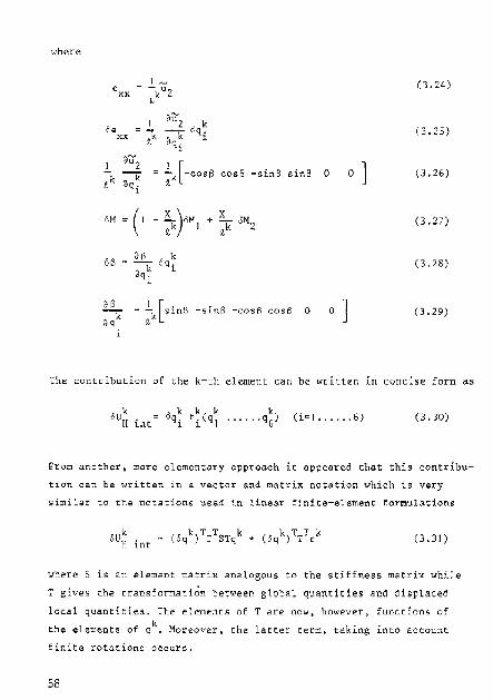
The contrihlltion of the k-th element can be written in concise form as

(i m ) ...... 6) (3.30)

PrUD another, more element~xy appxoach it appeared that this contribu­

tion can be written in a vector 8.n~ matrill notation which is ve,y

si,niiar to the notations used i.n li.near finite-element f.ormul8.tions

(3.31 )

wher" S i~ a,l element matrix analogous to the stHfness matrix ",hUe

T gives the tran"formati~n between global quantities and displaced

local quantities. The elem~nts of T ar~ now, howev~r, functions of

the elements of qk. Moreover, the latter term, taking into account

finite rotations occurs.

58

s = BF BF (3.32)

l ~k EF EF

- J\k J\k o o

1------+--. ------ .. -- ... - .. __ .. -l I

0 0 - £k .i,k

I I 7" ~

.. "-' ,-'" --------

tk lk

a 0 - 3E1; - bEl:

I,k - I,k - 6EI 3El

T = <oOa$ 0 sine 0 (3.33) 0

0 eosS 0 si.nS

-sinB 0 cosS a 0

0 -sinS 0 coaS

0 0 0 0 0

0 0 0 0 0

r = EF{I-cos(~-a )} (3.34) 0

-EF{I-coS(6-So))

0

0

6-80

B ~B 0

59

IE the n independent field values of the entire structure are col lec­

[ad in a vector q. we formally have

~qa (" = 1.2.".". n) 0.35)

where Lk is a matrix containing only elenlents 0 or I. For simplicity,

we assume all disc~ete field values to be free. In that case the first

variation of the Hcrrm'.lnn expression for the entire structure. bec.omes

where Q[1 are the generalized forces and rotations corresponding to q",

If we requi~e 6U yw O, this gives as many nan-linear equations as there

are e.l-ement~ qi.l:

(c., 8"1,2, ...... n) (3.37)

If 80me elements q~ are specified, their variations are not free and

a smaller set of equations will be obtained.

The non-linear equations can be solved by u5ing a ~olution proce.­

dure as described in Appendix Bt which implie.s stepwise incrementing

elements Q~ (and specified qR 's) and calculating the unknowns qB

by a linearized appro~ch. If desired, the ~olution thus obtained can

be improved by Newton-Rilphson iteration on the. set of non-linear

equations (3.37).

It can be seen from (.').32) that numerical difficulties are to be

expected when solvinA the non-linear equation" since th~ elastic

modulus E, being a large quantity, appears in the numerator as well

itS ~n th" d<)nominator of elements of S. Numerical diffj.~ulti.es CBn

be partly circumvented by eliminating E from S which is done by

choosing other VectOrs qk and Qk.

(3.38)

60

and adap~in~ the equations for the whole structure accordingly.

Wh~n iterating, the stopping criterion is that the increments of

the degrees of freedom 6q as ~ell as the residue Q~f(q) must fall

below a relative accuracy limit 0

(3.40)

A computer program has been developed which makes possible the

analysis of unbranched plane beam structures without moments 3t in­

t~rm~diate nodes. The major aim was to hav~ availabl~ a tool to pro­

dUCe numerical results Chat could illustrate the applicability of

mixed [inite elements for geometrically non-linear bending. Optimi­

zation of the program itself to save computer time was not 3imed ~t.

Details of the program are reported elsewhe.e 3.8

In order to demonstrate the applicability of mixed finite ele­

ments for geometrically non-linear bending, some numerical example,

will ~e presented. In vieW of the considerable computing time invol­

ved (some calculations took approximately 1 hovr on the ELX8) the

number of exarn?les will be limited.

'f';;'o different types of geometric .non-linearity will be demon­

strated.

Tbe first implies large displacements and rotations without

straining the axis of the beam t whereae tne se~ond implies finite

deflections while straining the axis of the beam gradually conrri­

but~s to the load carrying capacity.

The first example considered is a cantilever beam. acted v?on by

a concentrated rransveree force at the free end, This type of loading

61

can produce considerable displ,ac;eme.nts while the strain of the axis

of the be~m can be neglected with reap~ct to ehe. bending strain.

End diaplacements obtained (a) by using 5 elements Cas de8~ribed

1n Section 3,5) and (b) by applying the full load in 20 seeps and

iterating ~t each step (,eq~ired accuracy t ~ 0.01), are. compareo

wi.th an analytical ~ol~tion (numerical solution of the governing

diUerential e.quation) (Fig.3.3). The. example indicate~ that thi~

mixed approach produce" good results in the caSe of large displace-

mentS.

Fig. 3, J

~~- Dlfferen'tiCii'equot,on Present solution

End dhpZaaem(frlts of a oantiteve1" beam

The resul ts obtained will i)e influen.::ed by the n~mber of elements.

the mJmber of steps and the llCClJracy requirements when iterating. The

nlllnber of at"ps 00) is chosen arbin!'ril.y and the acclJ~acy c = 0,01;

62

the influence of the number of elements on end defle~t£on is ~hown in

Fig. 3.4. which indicates rapid and monotonic conve'gence.

\.0

0,9 I------l---+-

0.7

.!2

"2 o.s ~ :r: 0.4 .. u '0 0.3 " w

0.2

0.\

............ ___ .l-. ____ ._

..ff. .05 !linear) -E'TJ o L-----7---!::---!:;-.__. 5

Number of elemen'~

Fig. 3.4

Convergen~e ot end detreotion

V8rsus number of e&ements for

a oantitevep beam

rn the first example the behaviour of the beam was characterized

by large displacements caused by bending while the influence of

stretching was negligible_ Distinct non-linear behaviour can also be

obtained with finite deflections if the load carrying capacity due

to the bending stiffness is gradually supplemented by membrane action.

This can be obtained by clamping both end. of the beam_ After adapting

the elastic mod~lu5 E of the beam to ~ero strain in the direction

perpendic~lar to the plane of bending. the results are compared with

those of a clamped rectangular plate which is infinite in one direction

63

(Figs.l.S and 3.6). Since only results of uniformly loaded plat~8 are

available, the beam is also uniformly loaded. The von Karman eq~ations

of th~ plate problem hav~ b~~n solved by LEVr, using trigonom~tric

sarie. ~xpansions of the di~placem~nts and by YANG 3.9 using a finite

element formulation based on the pot~ntial energy principl~.

since the calculations of LEVY ~nd YANG were based On the VOn

Karman theory, in view of the underlying assumptions they are only

meanigful [or finite oeflections of thin plates. If the maximum de­

flection )s "max and tile ~pan of the plate is denoted by a, this

means that our own results may only be compar.d to those of LEVY and

YANG if w fa. c I. max

The reference cu~ves in Figs. 3.5 and 3.6 were obtained by copy­

ing illustrations p,esented by YANG 3.9

w h

'" .-:::.

::' c '2

~ 0; 't'l

1: c

'" U

64

2.5

;00

1.5

-- levy

!

I I

100

Pr~s~nt solution

I ' om: , I

i 300 400

Pressure ratio ~ Eh

J 500

CC"1/Y'(l d"fl.ectl:on for a damped h1["init(l $trip (,,=0.316)

fig. 3.5 presents the centre (point A) deflection versuS loaQ.

The n~mber of ~lements used for half the span was 10. The full load

pa4/Eh4 = 500 waB applied in 20 steps while we iterated after each

step.

The small dif£erence at h~gher loads can hardly be ascribed to

the number of elements, to the accuracy requirements made to the sol~-

tion or to the ratio between maximum deflection,

of the b~em, in view of the following results:

w • maX and span, a,

- with an acc~racy requirement of em 0.17. , a load level pa4

/Eh4 =

250 (10 steps), and wma~/a = 20%, we obtained:

number of elem~nts:

- with an accu,;-acy requirem~nt of ~ = 1%,

a load level pa4 fEh4 = 250 (10 st~p~), and wma/a = 5% ;

number of elements w h

max

- with a load level pa4/Eh4 = 250 (10 steps),

5 elements,

and w fa 20% max

Hccur.;LC

- with a load level pa4/Eh4 = 500 (20 steps),

5 elements,

w fa = 20% max

O.J % I 2.817

65

- wi.th ,~ load l~vd pa4

/Eh4 ~ 250 (10 eteps).

10 elements,

def l""t ion ratio 'IN /a 10% 5% max

accuracy requir~ment 0.11- 1%

wlt\a/ h 2.030 1.935

- with a load level pa 4/Eh4

10 el~lt\ellt:;;,

500 (20 steps),

an ac.~ura~y r~ql)iye.ment E: 1%

we obtained:

0'0' W

-?

~ ~

'"

deflection ratio w fa max

w h melx

IlU

--- Lt!'vy .------ Ym19 ;

100· ~ ~ 1'l"i?S~I'lt ~6lutlM

eu

M

'.0

20

°0 100 JoO Pr~~~ul'l':~ rc.J!io ...£..£.:..

Eh i,

2%

1 ~

1.931

I j ~~ /~

~+,r ~

..... Cl I.i •• , •

I.DO

~ i .j

i I

i

I

..... J 000

NormaZ-to-edge str-e.~s at mid-point' of edge of damped

1:,,{1:nUe Dtr-ip ('.)=0.:516)

66

Fig. 3.6 presents the total (bending plus membrane) .tress at the

mid-point (point B) of th~ long edge of the clamped infinite plate.

Agreement with the analytical r~sults obtaineo by LEVY is better than

with the finite-element results obtaineo by YANG, In our ~ase the

bending moments are primary variables of the variational formulation,

whereas in the formulation used by ~ANG the moments are related to

the second derivatea of the appro~imated deflection.

Since the bending atresses still dominate the membrane stresses

chis ~5 in favour of our Own calculations and those ot LEVY, and

might explain the differ~nce with those of YANG.

This example indicates that when applying the mixed finite-el~ment

formulation acceptable result~ for the diaplac~ments as well as for

the stresses can be obtained.

67

CHAPTER 4

Derivation o( the Herrmann (ormulation (or ti,e analysis of (inite deflections of plates

1,.1 intI"QductiOn

In Cl]apt€.r 2 tl,~ variational principlE'! of Herrmann has bE'!en

d~rived Eor tbe cas~ of large displ~cements of beams, while in Chap­

ter 3 two alternative procedure. were pre£",nted for formulating

finite-element models. The choice of theBe alt",rnativas depends on

the magnitudes of the displacements to be analysed.

In case of finite deflections the pertin~rtt simplifications en­

ahle U.';) to U$~ fixed local coordinate systel'l'lS, woe:'t'eas in case of

large displacements loc.e.ll coordinate ~yst.ems moving with the elements

can he advantageous. In the latter case, the form\llstion of the ele­

ment propert5~s relative to the movi~g coordinate system can be re­

(I\lced tD the linear f"rmulation, provided "len,ent dimcns).ons are taken

sufficiently small.

In th~ present chapter Herrmann'g variational formulation for the

analysis of the geomct~ically noo-linear hending of platRs will be

deriv~d. The same procedure will be used as presented in Cbapter 2

for the cage of heams. We will no~ confin~ our5elve~ to finite de­

flections since within thig range considerahle non-llne3hity may al­

ready OCCUh. Mor~over~ it covers almost all practical non-iTIfinite~i­

m~l plate deflection problems 4,1,

A different 8tartin~ point will be used in ~bis chapter:

In Chapter 2 we started from a large-di~placement potential ener­

ey formulation and obtained a lar-f,e-di.~placem"nt Herr-mann formulation.

68

The finite deflection formulation was obtained from the latter as a

spacial case in Chapter 3.

In the present chapter we immediately start from the finite-de­

flection potential energy formulation. The experience de~~ribed in

Chapter 2 does not make it necessary to in~orporate the shear defor­

mation in the starting formulation in order to distinguish between

two different stress displacement systems. In the case of finite de~

flections the proper formulation enabling us to discern between these

systems can be constructed directly. This applies eVen when the shear

deformations can be neglected, in analogy to the beam equations.

4.2 The potential enerzy formulation sui red to rhe transformation to

the Herrmann formulation

The von Karman 4.2 theo~y of finite deflections of plates will be

applied. Since in this theory the deflection is not assumed to be

small, a Langrangian description will be used. In chis description,

the Gr~en's strain tensor i. employed. Corresponding to this tensor

we have the symmetric Piola-Kirchhoff stress tensor.

Consi~er a thin, ftat, homogeneous and ~lastic plat~ of uniform

thickness h. We employ a fix~d Cartesian coordinate sy~tem, The Xl

and x2

axes are taken as lying in the middle surface of the plate in

its initial, unloaded state, while the x3 axis is taken in che ~irec­

tion of the normal to the middle surface, so that the xl' x2 and x3

axes con.titute a right-handed coordinate system (Fig.4.1)

For Xl and x2 we write xa(~=I,2) Or xa(e~I.2).

The plate ia aasumed to be simpl.y connected. The ~egion occupied by

the undeformed middle surface is denoted by A and the periphery of

this region by S. A coordinate s is taken along the boundary S. The

unit vector !. tangential to the edge ~ontour. and the outward nor­

mal n to this countour form a system of local axes in the xt-x2 plane,

whose orientation corresponds to a rotation of the axes x~ about x3

by an angle e, The components of ~ and! are:

69

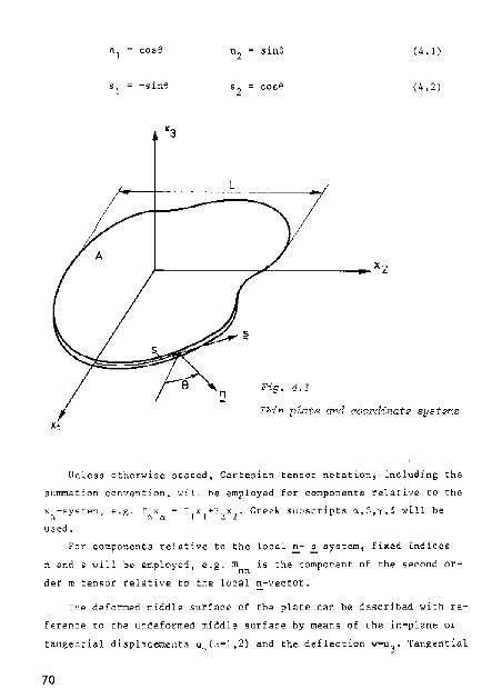
\1 1 ~ cose \1 2 sine (4.1)

s 1 -sine 52 cos~ (4.2)

)(3

L

f-----------~~~--------~~X2

Fig. 1.1

Thin r~at$ awi ('ool'dinate systernc

Unless otherwise stated, Cartesian tensor notation,. includi.ng th~

~llmmation convPrntJon't W1!.1, he employed for components relative to the

xc.-system j e.g. T~\xa - TtK1+1'2x2' Creek subscripts \.t,b,y,~ will be

used.

For components rehtive to the lo~al !!,- .:.. system, fiKed i!'lciiCeS

n ~!'Id swill b" employ~d, e.g. mnn is the component of the second or­

der m teTIoot rel~tive to the local !'I-Vector.

Tile deformed middle surf<'lce of the plate clln be descrlbed with re­

ference to the undeformed middle surface by mean. of the in-plJne or

tal1l:,entj.31 displ,'cemeno 11",(.=1,2) an.d the deflection w=u 3 , Tangential

70

displacements of m~terial points outsid~ th~ middle 8urfa~e, located

initially at Xi(i=l ,2,3) ar~ denoted by (d(~=1.2). The values of Xi

which define a material po~nt P in the undeformed plate remain fixed

tD P when the plat~ deforms. A surface derivative of a functiOn with

respect to Xu is denoted by the function, followed by a comma and th~

sub~cI'ipt I):

In the von Karman th~ory the following assumptions are made 4.2;

(I) The plate is thin. The thickness, h, is much smaller than the

typical plate dimension l, i.e. h«l.

(2) The magnitude of the deflection w is of the same order as the

thickness of the plate h, but small compared to the typical plate

dimensiDn l Le. 110'1 -&(h), Iwl« L.

(3) The slope of the middle surface is small everywhere, Iw,~I« I

(04-1,2) •

(4) The tangential displacements u~ are infinitesimal. In the strain­

displacement relations, Duly those non-linear terms which depend

on w'u are to be ~etained, All other non-linea~ terms are to be

neglecte<;[, Iw w.1 =&(u 0) (a,e~ 1,2) to. J I-l at U

(5) All strain compDnents are small, Hooke's law applies.

(5) Kirchho~f's hypocheeee apply; i.e., tractions On Su~faceB parallel

to the middle surface are negligible,

833

.. 0,

and IIlSterial lines which are origj,nally streight and perpendicular

to the middle surface r~main straight and perpendicular to the

mjddle svrface after bending.

With these assumptions a suitable potential energy formulation

will be constructed.

The temporary introduction of shear deformatiOn to make possible

prope~ di5cri~~nation between two ~tress-disp1acement systemS is

omjtted here, tn view Df Chapter 2, it i5 sufficient to distinguish

71

rotations of m(l.ceri. .• l 1 jnes "S menc~oned in a~~umption (6) as well as

slnpes of the middle surface.

We introduce the components of the sm"ll rotations of material

lines which originally were stt'3ight and perpendi.cul{tr to the middle

surface, ',«·'~I ,2), as ShOWII in Fig. 4.2. These components have been

so (,.ho!3en, tl-,at 'in vie'W of the se:(,ond Kirchhoff hypothesis dnd the

small, slop~s of th~ mi(ldle surf~ce we may write:

4',

j.

" w in A and on S (4.3)

Fig. 4.2

If t1 and 'r s ;:H-C the components in t11e n- ~ 5ystem~ the:: tr~nsformat.ian

i8

71

] n

:1, .... ~~ S (Ii. 4) S "1~"l

and the kinematic constraint (4.3) on S can be written as

¢ = w n ,n w

, s (4.5)

where ( ) ,n and ( ) ,s denote derivatives in tbe ~ and s directions

respectivily.

Displacements ~i (i'"I,2,3) of mate"da1 points outside the middle

surface are related to those of points of the middle surface by

(4.6)

(4.7)

The first assumption of Kirchhoff states

(4.8)

For the ather piola-Kir~hhoft stresses we define the following stress

resultants

+!h

N -o.S J -Ill

s"adX3

(4.9)

+!h

Q(:\ f so:iX3 (4.10)

-\h and stress moments

+jh

m .. r.6 -f saSX3dX3

(4.11 )

-!Il These quantities refer to the initial, unloaded configuration of the

plate. Since symmetric Piola-Kirchhoff stresses are used, NoS and mae

are symmetric. However, since all displacement derivates are small in

comparison with unity, the values of Noe ' Q(:\ and mr.6 are, in the first

73

order approximation, equal to the physical membrane forces, shear

forces and bending and twisting momentS defined in the deformed con­

figuration of the plate 4.~ The components of Q and m in the local n- ! system are

Qn Q n Q

s Qa~a a ex (4.12)

m ar m n n. m a m <:<6

n,/ e nn ~[l -:. Il n.

(4. 13)

ill = m -:-iR

s1:n

B m = m c<(l\,Se sn .5

In view ~f assumpti~n (4) of the VOn Karman theory the strain compo­

nents in the middle surface are

E. " = ! (u, ,,+uo ) + ! W W B :l~ );11:' I,'t a ,.0. ,

(4. ]4)

In addition we introduce the bending and twistin/t strains

I(.:d?' (4.]5)

The strain ener~y in the plate can be split into a part du@ to ben­

ding (Uint)b and e part due to stretehin~ (Uint)s

(4. ) 6)

(U. ) = f \ E c ~ dA lnt s A ry~y6 as yo (4.]7)

where A)6y8 ~nd E~d-;"yf are 8ymmetr;~ tensor~ c.ontaining lOCd.l stiff­

ness". of the plate

A - A yhl'

= A"cq6 A "~Oy

(4. ]8) ~i'yli

E '"[ly~

E y6-"e E[l.(y6 E ~B6~

(4. ]9)

74

The plate is acted upon by transverse pressure qO, ~y edge shear

loads VO

per unit length on p~rt $v of S, by edge bencting moments mO n ~

per unit length on p~rt Sm o£ S, and by in-plane forces per ~nit

length pO on S , Moreover, concentrated transverse forces pO. act at " p zJ

point 5j

of the boundary. If on a plate concentrated transvers~

fOr~e5 act ~t other points, then the plate can be divided into sub­

region5 having only concentrated forces at the bo~ndaries.

The loads are not specified as boundary conditions beforehand

because they will appear in the natural boundary conditions described

below. On the remaining parts the subsidiary conditions a~e respecti­

vely

0 S c S-SV (4.20) w w on

W

~n ¢o on S~ s-s (4.21 ) n m

0 S s-s (4.22) u u on

" " u p

With these definitions and the prevailing loads and boundary condi­

C~ons the potential energy functiona" ~s

-is m

-1 s p

p~ u ds - JE:pO.w. ~ j ZJ J

(4.23)

This !unctional,togecher with subsidiary conditions (4.3),(4.5),

(4.14),(4.15),(4.20),(4.21) and (4.22) forms the desired potential

ene,gy formulation becau.e two different di$placements can b~ distin­

guished, viz. wand t. This tormul~tjon is suited to the transforma­

tions to a Herrmann formulation.

75

4.3 Derivation of the Herrmann formulation

The potential energy form1)lation of the precedirtg ~~"tion l<i11

partly be subjected to Friedrichs'transformation in order to derivm

the pertinent lIerrmdnn formulation. Only the m-,¢ ~ystern will be

tr'\Il$f0rm~d. 'fo th.1t end all SUbsidiary conditions cOrttaining 1, vi7..

(4.3),(4.'),(4.15) and (4.21) will be introduced into the functional

by mean; of multipliers. Ih. remaining SUbsidiary conditions are

(4.14),(4.20) and (4.22), becaus~. these belong to the system which

pr~serves its potentbl energy form1)lation. As a consequence of our

re"lriction to finite deflections, the SUbsidiary conditions which

dre introduced into the functional are line3r, so th.t the Friedri~hS'

trBn5fo<matlon will he applied to d line~r bending system. The Whole

ge.ometrlc.al non-linearity is embodied in condition (4.14), whi<:h will

nat be subjected to the transformation.

The idcnti.fication of the muHipLier~ i~ given 1n Appendil< C.

After introduction by means of the identifi.d multipliers of th. COft­

sttaints to be removed, functlon.l (4.23) hecomes

- i[ m (,p -w )ds J~ ns l:- I g

o l' .w.

Zj J (4.24 )

The se(,.ond ~t.p, a. mentioned in Section 1.3, implied e"pTes~ing the

~train "'=:."1 in the moments !Ilt).S"lf we: re:Ciuire ~KU2L:10,. this give. s

(4,25)

76

This relation ia invert<!:d

(4.26)

and used to repla~e the scraina ~aS by a~re5S r<!:5ultants m~S

~ [I Ao:ayli"~e'\1i - mae"ae}iA = ~ - ! BCI~y6m",Smy6 dA

(4.27)

Introduction of (4.27) into U2

(4.24) would give an expre~5ion ana­

logous to U3

in Section 1.3.

The third step implied partial in~egra~ion 5uch that the moment equi­

librium equation appears, analogous to (e 22) and (e 23) in Appendix

C. This, together with (4.27), tran~forms U2

into

-1 m a 0+ Q}¢ JdA-1 0:"," 0: C! S V

-Is p

(4.28)

If we require equilibrium of the moments

m«s, e + Qa 0 in A (4.29)

0 S m em on (4.30)

nn nn m

the functional becOmes independent of the displacement ~a of the

system w<!: wish to treat complementarily and of the fort~ Q" of the

system we wish to ~reat according to the principle of potential

energy. We thus ob~ain the Herrmann functional

77

- Lr~jwj j

P~ u ds +JC m $0 I) 5 t nn n d" + i

s m w os +

nS ,~

(4,) I)

The remaining sub5idiary condition is (4.30) tDgether with the origl-

nal subsidiary condition. which w~re not subjected tD the trart~form~­

ti0n:

.. j(u +v ) + ! In W in A (4, 14) ", ~ .\ , ~~ (~ ,. ~j, ." ,I;

= " S (4.20) w w On w

0 S (4. ZZ) u u On

" U

Ihe quantities subject to v.rl~tions are u~.w and m~B'

4,4 Correctne85 of the formul~tion

Tbe c"rrectnes, of th" preceding formulation will be proved by

comparirlg its stationary conditions with the gov~rnin8 equations (e.g.

WASlIHlI 4.3).

The 9tationary conditions with respect to un'. ~nd Ul. r will be

derived con5e~utiv~ly.

whe.re

78

'\ Uti = l [F.:dYO ":d, 8 u celS] dA - is p

(4,32)

(4.33)

lntroducing the stress-resultants N~S

and using the symmetry in ~ and B. the first term of (4.32) becomes

Hence. the stationary conditions of (4.32) are

N = 0 «a." in A

on S P

(4.35)

(4.30)

(4.37)

(4.38)

Eq. (4.37) expresses the equilibrium oe £n-plane forces while (4.38)

expresses the dynamic boundary conditions of these forces.

Variation of w gives

(4.39 )

By proceeding along the same lines as in obtaining the stationary

conditions of (C 10) in Appendix C, the !ollowing stationary con­

ditions are derived

o in A (4.40)

- m - 2m + N w + N W vOn on Sv nn,n us,s nn ,n ns ~s (4 .4l)

79

H m OS

o p .

ZJ at. points (4.42)

Eq. (4.40) ""pr~s~"s lb.e equilibrium of forces in the w-direction;

In view of subsidiary condition (4.29) - maS,S equals the shear

load, Q~ while the in-plane [Drees NaB acting under a small slope

w ~lso contribute. , K

rn Cq. (4.41), (-m -2m ) is the dfective shear force known nn,n TIS,S

from th~. 1 inear theory. Tn this non-l inear case the in-plane forces

Nnn

and Nns

alSD contribute in the dynamic houndary condition. As o

in the linear theory, concentrated transverSe loud. Plj , cause dis-

continuity in the twisting moment mns

' as expressed by (4.42). All

stationary conditions obt~ined so far are in accordan~e with th@

governing equations Bnd B potential energy approach.

Finally, variation of m2B

gives

~ ([ ~ em d~ + f to om ds .J~ "s ns S n nn

(4.43)

¢

In view o[ (4.26), the "tationary conditions are

W , f). ~~

K C'le in A (4.44)

W ¢o ,n n on 8~ (40.45)

Tb.ese are the compatibility equations as can be e~pected from a ~om­

plcmentJry energy opprodch.

4.) Alternative finite-element models

With the preceding Herrmdnn formulation ~ariolls fil)it",~elcment

models can he constructed. depending on the definition of the inter­

action between neighhouring element. and the choice of the local ap-

80

proximating fun~tiens. Up to now it was ta~itly assum~d that the

fi~lds we~e continuous and had sufficient partiaL derivatives to

make possible eQe per~inen~ derivations.

In this sect£on the proper~ies of the fields will be ~onsidered

more closely hecause they are important when constructing app~oximate

solutions by means of the finite-element method. As described in Sec­

tion 3.2, this method implies a division of the Whole domain A into

subdo~ins, Ak, the finite elements with bounda,ies sk. Superscript~ k denote element numberij. The true solution of ehe variational fo,mu­

lation inplies continuity of quantities as appear in the natural

boundary conditions, viz. rotations and stress re5U~tants. The sub­

division into elements should not violate this continuity at element

boundaries. Insight into the ~elevant quan~itieB and the requirements

to be made can be obtained by dividing domain A in functional (4.31)

in~o subdomains, and determining ~Qe stationary conditions. If we are

agreed that th~ integrals containing prescribed quan~ities must be

tak~n over the relevant element boundaries, then the fun~tional

becollles

-1 s p

m W ds _f VO w de + ns ,s J

S n

m ~o as nn n

V

- m. \Ii + all. e ,(1

(4.46)

To obtain the stationary condi~ions, the operations mentioned in

Se~~ion 4.4 must now be performed for each domain. Then the Euler

equations (4.37), (4.40) and (4.44) will be obtained for each sub­

domain while fo~ eLemen~ boundaries coinciding with the relevant

parts of S of the·whole struc~ure the natural houndsry condition"

(4.38}, (4.41},(4.4Z) and (4.45) will be obtained.

81

For all {nter-el~ment boundarieB where the variations are free,

te.rmR will "ppear which are identical with the I,eft-hanct members of

the natural hound~ry conditions and multiplied by the relevant va­

riation of the element concerned. If, for instance, we observe the

boundary between elEment k and k+l, which extends from node I to

node 2 (Fig. 4.3) we obtain the terms

2

f (4.47)

]

f2

l (~m - 2m ! k k + N w + N w )ow ds + nn,rt t'l.S, S nn ,n ns 'I'M:

]

]

{l (-m - 2m + N nnw'n + N w )ow} k+Jd/+1

2 nn,n l;1~'1~ n,s ,s

(4.48)

(4.49)

wher.e

k k+] ds - - cis (4.50)

It .hould be noted that variations of the twisting moment, omng , do

not appear in these term •• Continuity of the in-plan~ stress re"ul-

tants Pc); NI)L~J"J.,~, eff~(:tive. shear farce Vn (-mnn,n - 2mns ,s +

Nnnw,n + Nn."".) and "ormal slope w,n o"er element boundaries will

only be obtained if we require ue' wand mnn to b~ ~ontinuou~ acro~s

element boundaries. (:ondnul.ty at: mns is not a requirl!.ml'!nt.

Anot]l"'" app~o"ch, involving severer requirements, is obtained if,

1n addition to th~ ~bove, we require the twisting moments ffins to be

continuous across eeemellt boundaries. Then, since we already required

w (and thus w,o) to be continuous, we have in (4.46)

82

Ne

'Lfsk mnsw,s k=1

and (4.48) become~

ds = i s

m ns w ds , s

j 2{(--jtJ -m +N w +N w )6w 1k cts k + 1 nn,n ns,s nn,n ns tS r

(4.51 )

+11\(-m -

2 nIl,n f k+l k+1 m + N w + N w )~w ds nS~5 nn tn ns ~5

(4.52)

Thie cen be written as (compare (C 20»

J~ I

(Q + N w + N w )&w k dsk +

n nn ,n IlS ,s

(Qn + N w + N w )6w k+1 d.~k+1 nn ~n ne: t S

(4. S3)

In this case, continuity of w ~uarantee" ~ontinuity of the vertical

force resultantS (Q +N w +N w ) instead of the effective shear r'l. nn ,n nS ,5

fol"c.es V • n

Fi~. <1.5 Boundary between two domains

The simplest triangular element fulfilling the latter require­

ments can be obtainect if for each elemeIlt linear approximating fields

83

ul,W and mCl0(=m~~) are chasen, each uniquely definad by its discl:ete

values at the angular-point nodes. This implies an element with 18

di~crete fiel.d V(l.l\leS (Fig. 4.4),

{m)()(} myy mxy 1

Flg. 4.1

{ffiXX} myy

mxy 3

w2.···_····_lJ 2 {m)()(} myy mxy 2

Tf the requirements made on the moment fields are restricted to

cOlltinuiLy of the normal moment !linn' a cOnstant moment distribution

can he c.ho~en for the appr~"jm .. ting f.unctions b"cau~e the three

mnments mxx' myy and mxy c~n be uniquely expressed in the normal

moments t\\oo at th,:, thy",,,, sid~s of the triangle (Fig. 4.5).

M{xe;} pr.ate-/)m,dhlg (Ji.ement with 12 d{sQl"cce fidd val.ues

84

In that case the local approximating functions can he expressed

in 12 discrece field values.

In ~omparison with plate-bending elements as used in the poten­

tial energy formulation this means a considerable 5implifi~ation

while it is not difficult to formulate el~ents consistently with

the ~ontinuity requirements.

Within the linear domain. HERRMANN 4.4 obtained good results by

using the elements with complete moment continuity as well as by

using the simpler element with only normal moment continuity 4.5

OwinS to its simplicity the latter element w~11 be used in our

non-linear formulation.

85

CHAPTER 5

A mixed finite element for the analysis of plate bending

5.1 Intl"ociuctio[l

In the preceding ch.'pte.r th~. c.ontinuous Herrmann formulation [or

the. analysis of finite deflections of plat"" was obtained. 1n the

pre~ent c!lapter this formulation will he used to construct a finite-

~lement model. ()f the two models mentioned in Se~ti.on 4.5 the. second,

having 12 degrees of freedom, is chosen because this restricts the

number of unknowns to be solved for the entire Styucture compared

witll othe.>:" element models and the same subdivision of the struc.ture.

The tensor notation of tlle continuous formulation will be recast

in a matr]x notation for the discrete e1.ern~_nt model., acc.ording to

the procedures useo by aERGAN ano Cl"OlJ(;H s. I In the ) i.near f ini te­

element formul,at;ions vectOj; ~nd matriJ< )'1.ot;ationg have hee.n widely

accepted and special prDcedures. e.g. for data handling and assembling

the finite elementRI have been developed. By adopting Q vector and

ma.trix notation for our noo-linear formuiation l experience and prot:e .....

dures of the linoor formulations con be used for the ~ornputer pro-

gramming f

5.2 Form1.<latfon of the finite-element; model

We consider one element of the entire structure. The element of

Section 4.5 with 12 degrees of frBedom requires the di.spl"~ementR u('

.and 'tJ .:;1.$ well 03S the normP.1l moments r1.1 to be c.ont.jnI.)Oll8 BCrO!;l~ the nn ~lement. honndaries+ The line03.r displa~e.ment dil3tribution c.an uniquely

be defined In terms of their v~lues ~t the angular points li(i=I,2,3)

86

of the triangle. Continuity of displacements between two elements

witl be obtained if the di~crete field value~ at the cammOn node~ are

equal.

Jhe constant moment distribution can uniquely be def~ned in term.

of the normal moments mnn at the side. of the triangle (Fig. 5.1).

Continuity of the normal moment will be obtained if the values at the

common side are equal. In order that the approach shall be consistent

w~th the finite element approach, we introduce nodes '\ (i=I,2,3)

halfway sides of the triangle and denote the discrete field value

of the normal moment at that node by mun,'

The eequence of the numbers of the nod.es has been Chosen 1n accor­

dance with our right~hand coordinate ayetem.

Throughout this chapter the following notation will be used:

Instead of the independent in-plane coordinate. XI and x2 or the

preceding chapter we uSe x and y.

Instead of the in-plane displacements ul

and u2

we use u(x,y) and

v(x,y),

Fielo quantities will be foltawed by their independent ~Dordinate6,

e,g. ",(x,y).

Di$crete values of field quantit~es at nodal points will not he

followed by the independent coordinates but will have as subscripts th~

numbers of the relevant nodes, e.g. ul

is the displacement in x~oirec­

tion at node J.

Tensor components remain identif~able by their Greek subsc~ipts a,

(free indice~) when referring to the ~Dordinates ",y or by nand s

(fixed indices) when referring co the local coordinates n,s.

Matrix notation will be used. Vectors are considered to be parti­

cular matrices ao that only their definition will reveal whether they

~re a row or a column~ e,gf if

w =

87

y

z ----------------------------------~~- x

y

z .-----.---.--.. ----------.--.--.. -- ... - -... -x

Fig. 5.1 Tr"iangulap plate-(.'iPidin.g Bl&ment with 12 dir;"p$t& [{do'!

valueD

88

then

The following geometri~ quantitie~ will be used:

Th~ 1~ngth5 a£ of the ele~ent sides are given by

i :- 1,2,3

j:= i+1 if i=l,2 j:= if i~3

If Si is th~ angle between the normal ~i on side

we have th~'follawing relacions

X.-x . 5in Si .2:..-L = n yi s xi a.

1

Y,-x, cas S. ..L..2:. n .. s

l. "'-. xi yi L

(~.I )

(5.Z)

and the x-axis

(5.3)

0.4)

where sxi and Syi are the ~omponents of the unit ve~tor tangent to

side i while i and j must be chosen in acco~~ance with (5.2).

The ~hosen local ",-pproximating fields will now be exp~e5sed in

their discrete values.

The linear distribution of the deflection w(x,y) is given by

w(x,y) .. [I xc (5.5)

where

(5.6)

89

(5.7)

We collect the nodal point defl~ctiong wi in a Vector w

(5.8)

The coafficiant~ Ci are expressed in the wi by

c = T " (5.9)

where

T 2A [ ""~lY' X 3Yl-X 1Y3 "'2-""1 0 ['ill Y2-Y3 Y)-Y 1 Y1-Y2

"3->:2 XI-)L~ x2-x

l (5.10)

Combination of (5.5) ano (5.9) gives

INC", y) XTw

or l in concise form

W(",y)

where

<I> w w

(5. III

(5. 12)

(5.13)

(5.14)

The linear distribution of the in-plane dj.splac:e.ment~ u(",y) ana v(x,y)

~an ba e~pre5sad analogously. We treat them simultane.ously.

We collect the in-plane nooal point displac:ement5 in a vector v

90

(5.15)

Analogously to (5.12) this gives

[:::::H: :] [: :], (5.16)

[U(X,y~ V(X,y)J =¢ v

v (S.17)

where

[X'I' 0 1 o XT

(S.18)

The rel~t~~n between the ~onetant rectangular components moe

(~ea) and the di5~rete values of the normal moments mnni associated

with node. J i ~an be obtained by using (4.11):

(~=x.y and ~=x,y) (5.19)

These three relations can be written as:

(S.20)

We define

(5.21 )

91

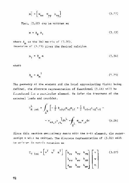
l' r m = m 1 . xx

Then, (5.20) c;<n be wdttep. as

where Am ~B the 3x3 matrix of (5.20).

Inversion of (5.23) gives the desired ~elatjon

ill) B m m

wh .. r~

B = A -)

III m

(5,22)

(5.23)

(5.24)

(5.25)

The geometry of the. element and the local approxim~tin8 field~ being

defined, the discrete representation of functi0n~1 (5.46) will be

formulated for a particular element. We defer the tr.,.?tment of the

exte.rnal loads ~nd ~onsider.

1)Hk

int

m TN d~ TIS ~ So

(5.26)

sinc,;, this section el<clusively deals with the k-th element, the sl)per.­

script k will be omitted, The discrete representation of (5.26) will

oe ~ritt~n in matrix notation as

u = [vT T .'] [> k H inc w vw

k wv ww

k k m" mw

(5,27)

92

wh~re the submatrices may be functions of discrete field values.

(al The disc~ete representation of

proceeds as fol1o~s:

rf we ~est~ict ou~selves to an isot~opic material, this eontri­

but~on can be written as

(5.28)

where

'". ru;" _; 12 [ (5.29)

Using (5.24), this contribution can be expressed in m (5.21)

(5.30)

so that the followins relation is obtained

(5.31)

where

(5.32)

(b) The discrete representation of the membrane strain energy

93

94

with subsidiary condition

I + - W <:.N

2 .,,-,8 (5.33)

proc .. eds as follows: Since (5.33) cosists of a linear al~d ~ non­

linear part we define

T [dU 3v (1) b:] (5.34) f. ay -+ I .. . d]{ dY <Jx

T wwr (dW)2 2 3", ~J (5.35) " NL L \"" "Y "" dY

With these linear and non-linear strain vectors we can writ~.

where

(5.37)

We define the fQl1.owing matrices

(5.38)

w = [w 0] () w

(5.39)

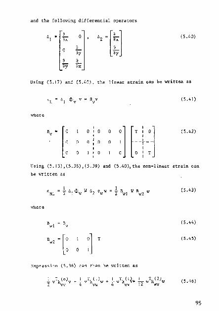
and the following differential operators

Ie. ~ [L 0] Ie.~ = [L] 1 ax '~ax

o L ~ ~y ily

a a ~ ax

(5.40)

Using (5.17) and (5.40), the linear strain can be written as

EL ~ ~I ¢v v .. B v v

(5.4] )

where

][ , 1 '. "l C

0 0 a a T I 0

• 0 0 0 0 0 1 --t~-0 0 I 0 o 0 I T

I

(5.42)

Using (5.13) ,(5.38) ,(5.39) and (5.40), the non-linear strain can

be '"'1:"itten as

(5.43)

where

(5.44)

"(: : :], (5.45)

Bxpression (5,36) can then be written as

(5.46)

95

where k(o) T

DII R A (5.471 ~ B vv v v

k (I) ~ C

I W whh G

l T (5.48)

VI' Bw2 A BV 0Il Bwl

k (I) BT wI CI A (5.49) wv w2 I

k(2l 3 T W

T G W Bw2 A with G 81

DII Bwl (5.60) ~ - B WI' 2 ..,2 wi

The superscripts i~ parentheses denote the power of the discrete

field valu~s app,,~rinS in these matrices.

The first term of (5.46) is quadratic in the in-plane displa­

cements v and respresents the ~trai~ ener~y due to memb~ane

stretching without deflection. The last term represents the strain

energy due to membrane stret('hing caused by deflection, and the

other terms repre~ent the coupling between in-plane displacements

and deflec t ion.

(c) wi til the chosen constant moment distribution we have

o (5.61 )

(d) Next, the contribution

96

In W ds ns tS

will be expr.essed in nodal-point quantities. Tne assumed fiElds

imply that hoth mns and W,s 3re constant along eacn side. Tf we

collect the leIlghts a i of the sides is a matrix P,

(5. (2)

w~ C.an write

m W dS"[W nS ~ s ,s: [ "',53] F [:n81]

n.2

mns3

"',52 (5.63)

where the tangential slope .. (w,~) along side i c"n be expressed

in the discrete deflections w. and the twisting moments m . 1 nSl

along side i in the discrete normal moments mnni .

The twisting moments mnsi

can be e~pressed in the Cartesian

components mae by means of (4.13)

mnsi ~ maS n~i sei (5.(;4)

lm ~ ~_"m', <,-osSI sinS

I cose

l '.,"'] l::r'" m:: = -s~nB2 cosS2

sinez cosS. cos 2 S2

mns3 -unB3 cose} 5~nS3 <;0 58 3 00 526

3

(5.66)

In view of (5.24) the Cartesian components collected in WI Can be

expresseo in the three normal moment~ along the sides oollected

in m. This gives

[:""1 D II m

m

ns2

mns3

(S.P)

For the tangential slopes we have

w = w s + W 5 - w "inS + w cOs S ,5 ,x x ,y y ,x IY

(5.68)

97

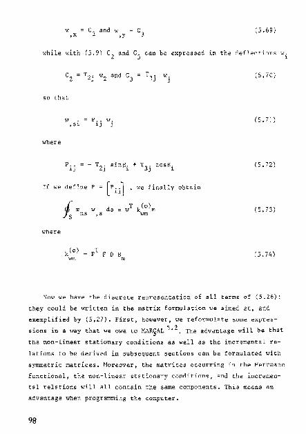
(5.69)

while with (5.9) C2

and C3

can be exp~essed in the deflection~ wi

50 that

where

w . ,s 1

If we def ine

Is m ns

where

p,. tv. 1J J

p [p i.i] "I cis , "

w. (S,70) ]

(5.71 )

(5.72)

, we fi.n,~Uy obtaj.n

T k(o)m "I

wm (5,73)

(5.74)

Now we h~ve the di5crate repr6santation of all terms of (5.26);

they could be =itten in the matrix formu1.3tion we aimed at, and

eX<i!mplified by (5,27). First, howeve~, we refo:r:ml,lJ.~t<i! 50rne expre,;-J 2 . h aions in a way that we Owe to MARgAL ' , The advanto.8'" w111 b<i! tat

the non-lin<i!ar stationary condition. as well as the incremental re­

lations to be derived in 51,lbsequent section. can be formulated with

symnletric matrices. Moreover, the mat-.:ices occ\ITring in the Herrm8I1I"l

functional, the non-linear st~tionary cooditione~ and the increm~n­

tlil ,elations will aLl contliin the ?ame components. this means an

advantage when programming the computer.

98

Since k(1) vw

Using the definition of k(1) (5.49), the last te.m is wv

(5.75)

(5.76)

In view of (5.41), D1 1Bvv represents the membrane forces N~, Ny

and N~y i~ absence of deflection. If these are collected in a symme­

tric matri~ 00'

rj - [N N 1 0. ~ ~y

N N y~ Y

(5.77)

Eq. (5.76) can (see Appendi~ D) b~ reformulated 1n the symmetric form

(5.78)

wheL~

(5.79)

By collecting the individual ~ontribution5 of (5.26), the discrete for­

mulation for the element becomes

UH int = [vT wT rnT] 1. k(O)

2 vv 2. k( 1) 6 vw

0 v

l k(1) 6 wv

2., k(l)+ 2..... k(2) 6ww 12ww

2.. k (0) 2 WIll

w

a 1. k(O) 2 row

_ 1. f(O) 2 III!Il

m

(5.80)

99

Subruatrix f(o) represents the bending strain and is positive definite. mm

Since in (5.80) - t f~) appears, the combined matrix cannot be p05i~ tive dcfinitf!.

5.3 The contribution of prescribed loads and rotations

An etdditional contl:"ihution to the Herrmann functional (4.46) is

effected if an element is loaded hy a distrihuted load qO or if an

element boundary coincides ~ith a part of the structural boundary

where loads or normal rotations are prescribed. If the prescribed

quantities together with the assumed approximating functions are

introduced into the functional,after integration this leads to g"ner~­

lized quantities associated with the discrete values of the approxi­

mating functions.

We define a vector wi.th gener a li 7.ed quantl t1 es pO., pO. and pO. Vi Wi ml

1n such a way that for th~ ~l~ment th~ contribution of prescribed

loaes and rotations can be written as

T w (5.81 )

If we assume the distributed load qO on the element with surface

area A to be constant, this gives

(5.82)

I 0 '3 q A (5.83)

are the generalized transverse loads associated ~ith angular points

Constant edge shear loads VO along side n

contribute to pO~ w

100

hounded by nodes and

1. VO a, 2 n 1

(5.84)

Con~entrated transverse forces po_ ean easily be taken into ZJ

ac~ount if the element distrib~tion hes been so ~hos2n that ang~lar

points ~oincide with the points of appli~ation. Their cont~ibution

pO is w

(5.85)

o 0 Assumed in-plane for~es per unit length Px and Py along side

COntribute to pO V

(5.86)

with k c i+3 ~nd t cj+3

A prescribed ~onstant rotation ~~ along side

ralized ~otation associated with side node i

le-ads to a gene-

C'5.87)

If ~or a particu~er problem theSe assumptions are not e~ceptable.

thon genorali~ed quantities appropriate to either other ass~mptions

or the actual distribution can be obtained by introducing the rele­

vant distribution into the ~unctional. It is useless to eombine com­

plicated distributions of specified loads and/or rotations with simple

approximating functions for the displacements and/er the moments.

5.4 ,he contribution of one element to the non-linear esuation~ of

the entire stru~tur~

In the pr~cedi~g s~ctions the element was considered disjoint

from the structur~ wh~n formulating its contribution to th~ Herrmann

expr~$sion of the entire structure. This was possible because the

101

local approximating functions are \1\li,ql,le1y defined by their discrete

values at nodes pertaining to the. relevant element. To be able to

distinguish an arbitrary element witl: 1I\1l\1ber ~ from the entire struc-

ture~ we ag~in introduce the superscrint k. Th~

ly "on"i5t5 of two parts, a contribution due to

(5.80) and one due to sp~cified external forces

contri~ution general­

internal forces UHk

int and/or rotations

u~ e~t (5.81). For the entire structure we then have

UH ~ L u~ int + L::u~ ext (5.88)

k k

The non-linear st<ltionary conditions ar" obtained by requiring I\UH=O:

o L (5.89)

k \c

T11US ",e can st<lrt considering the contribution of an arbitr(l.l:"Y element

and defer the ~ummation of che individual contributions, i.e. the as­

sembling of the non-linear equations of the entire struct~,e.

By taking the first var~ation of uK. (5.80) with respect to all k k k H lnC

components of v • wand m • and by transforming the reRu1t in such a

way that component matrices become free from variations (see Appendix

1) We obtain

r rr auk , = [6V1" owT 6m

TJ K . k (0) .!. k( I) o v H ~nt vv 2 VW

I l! k(1) .!. k(I)+ 2.- k(2) k~T · i wv 2 ww 3 WW

0 k(o) -f;;) l m

mw

(5.90)

~

The submatrices contai.n the ~ame constituents as the Rubm<ltrices of

(5.80). Only the cocffi~ients have ch<lnged. The sq~are matrix sO ob­

t/lined is an;ltlogous to the element stiff.ness matrix in displacement for­

mulations. In this case, howe.ve.r, the m~tri)\ contAins also flexibility

102

te~s in f(o). ~~d geometric term~. e,g. in k(O~ Thus it is not allowed IIIIIl """

to ~se the name stiffness ma~rix. We call it the non-linear element

matrix. The components ~ k(l) , l k (1 ). + k (1 ) and * k(2), which are ~vw 2wv ~ww c.WW

functions of displacements. constitute a matrix which is analogous to

the 50-called geometrical stiffness matrix in the formulation entirely

expressed in displacements.

If the element is subjected to external loads or prescribed rota­

tions, then it also COntributes to the external potential UH

ext of

the entire structure, Thi. contribution was written as u~ ext(5.81).

The first variation is

wk H ext

[T , 'Tl' o - 6v "', :~ (5.91)

If we define the vec.tors

k! [ v

T T mT] k q w (5.92)

QkT = [p~T poT w

OT] k Pm (5.93)

we can \lit"it~ (5.90) and (5.91) in concise form as

Wk H int

.. oqkT f k (qk) (5.94)

oull H ext

ok! - q Qk (5.95)

where fk is a vector with non-linear eql.lations in tD'" ~nknooms collec­

ted in ve~tor qk. If the structur~ consist~d of one element and we

requi~ed 8U~ = 0, this would give the following set of non-linear

~lement equations

(S.96)

103

In Chapter I) it will be described how tllese non-linear ele{llent COn­

tributions c.all be assembled to form the Set of non-linear equations

for the entire ~troctllre.

5.5 The contribution of an element to the incremental equations of

tile entire structure

The nDn-lin~ar stationary equations of the entire structure will

be solved by a method which implies a stepwise procedure as well as

iteration (5"" Appelldix B). Apart from the goVel."Oillg non-linear "w"a­

tions, this procedure requires linearized incremental eguations. As

in the preceding section, we first focus attention on an arbitrary

element. The incremental equations of the entire structure can be

assembled by means of th" iIlcremental eguations of element;~ once

these h<lv" been formuJated.

Formally, the incremental equations of an element can he obtained

by applying a fir"t order Taylor expansion on Ehe governing non-linQar

Rqu8tions (5.96), a, described in Appendix H.

If qk is a solUtion to (5.96) corresponding with Qk and if qk+L\ql(

is a solution CorrespDnding with Qk+6Qk, we llave

1£ we suppos" fk(qk) to have partial derivatives with respect to all

components of q\ we can e:><p"nd the l"ft-ha[ld member of (5.97).

(5.98)

where

Then, in vi"w of (5.%), the linearized inCTemental ",quation lS

(5. 100)

104

1n our case, the incremental equations were obtained by taking the

difference between (5.97) and (5.96) and retaining only term~ whi~~

ar~ linear in t,qk If we introduce the matrix formulation, apply this

procedure and modify the result in such a way that w~ obtain a square

matrix which is free from the increments 6qk (see Appendix D), we ob­

tain

.... o l k(o) \>(1) k 6v k llpo k (5,101)

'IV vw v

k(l) k(l) + k(2) k:' J ~w ~ lIFO wv ww ww w

0 k(o) _f(o) llm 6po mw mID m

The ~onstituents appearing in the square matrix are precisely those

of the Herrmann expression (S.80} and ita first variation (5.90).

This simplifies the computer programming of the non-linear and incre­

mental equations. The square matrix appearing in (5.101) will be

called the in~rernent81 matrix.

105

CHAPTER 6

The equGtions of the entire structure. the computer program and a numerical

example

6.1 Introduction

In the preceding chapter we formulated a mixed-type finite ele­

ment "'ith 12 discrete field values. The contribution of Buch an ele­

ment co the nOn-linear equations as WEll as to the incr~mental equa­

tions of the entire structure "'as derived. While doing that all dis­

crete field values were ~ssumed to be unspecified.

In the present chapter the entire structure is be considered. The

contribution~ of the individual element6 will. be asserr,bled to form

the set of equations for the plate to be ~n~~yze0. Since in this case

displaCements and/or moments may be specified beforehand, this implies

that ~Qme dis~rete field values may now be sp~cified.

The major features of a computer program for the analysis of geo~

metrically nOn-linear bending of initially flat plates with an arbi­

trary shape and arbitrary boundary conditions will be given.

Some numerical ~esults obtained with thi~ progr,3m wi 11 be com­

pared ~ith known other solutions.

6.2 The equations of the entire structure

In Chapter 5 the contribution of a particular element to the

llerrmann expression of the entiro;, plate waf; preoented, The (lisc);-ete

lle1;J;"mann formulation for the entin' plate can now be obtaineo by

adding the contributions of tbe individual elements (see (5.,6))

(6, t)

106

where uk Contains the ContributiOns of distributed loads qO, H ext

6pecified cOncen~rated for~e8 pO, acring at angular points, and of ZJ

specified edge forceg and edge rotationg.

The nOn-linea~ equations to~ the entire plate are obtained by

requiring that lUH

= 0

o L (6.2) k

the ~lement contdblltions (5.90) and (5.91) can be "r;ltten in ~ondse

form by introducing the vectors with element discrete field value~ qk

(5.92) and with element generalized lo~d~ and rotations Qk (5.93) • If

we d~note the square matrix which appears in (5.90) b kk Y qq this gives

cull. d kT kk k (6.3) )1. lnt q qq q

6Vk H ext

_ 6qkT Qk (6.4)

For convenienCe and to be independent of the plate to be analyzed.

the nodeg and discret~ field values of the element have their. oWn

local numbering (see Chapter 5). If, however. a plate '6 divided into

finite elements, the nodes and discrete field values of the plate

have a global numbaring. Thus, the ~ontribution~ of each element must

be expressed in these global discrete field values.

If qk are the discrete field values of the k-th element and q

those of the plate, we formally have

k Lkq and k L k6q q 6q (6.5)

Coner i bu dons (6.3) and (6.4) then become

k ~ <sq' LkT kk Lkq CUn int qq (6.6)

wk H ext

6q' Lk1 Qk (6.7)

107

Int,oduc~ng ch~s into (6.2) gives

(6.8)

We define

K = L I,kT kk Lk qq j( qq

(6.9)

Q = L: J,kT Qk (6. I (I) k

wheTe K 15 the system'" nl<ltrix of the entire plate with reference to ~q

all dis~rete field value" contained in q and Q is the vector con-

taining all genet.lized farces and rotations.

As a consequence of our matrix notation, the assembling of Kqq

and Q can proceed in the same way as the assembling of sti.ffne.~s

matrices and ~ummation of generdli~~d lOcids of the elements in the

linear displacement formulation a~ described by VISSER 6. I with de­

finitionB (6.9) and (6,10) the stationary conditions of (6.8) can be

written .a~

Q (6.1 I)

where the ~omponents of K are functions of componenta of q. This set qq

of non-linear equations for the entire plate can also be written ao

f(q) = Q (6.12)

where £ is -I' ve<;tQr with non-linear equations. This set of eqlJations

can be solves by means of a 1insarized incremental appro8ch alter­

nated by Ncwton-Raphaon ;teration. If llq is the increment of q and M)

the incJ;"ement of Q, according to Appendix ll, the formulation s\lited

to this approach is

Klqq

6q ~ ~Q + Q - f(q) (6.13)

108

where K1qq

is the incremental matrix of the entire plate, defined by

(6.14)

When itllrating, ':'Q~O.

If we denote the incremenCal etement matrix apPllaring in (5.101)

by k~qq' th~ matrix Krqq can be assembled by adding these individual

element cont~ibutions.

(6. 15)

Up to now, all components of q were a •• urned to be f.ee. If compo­

nents of q are specified beforehand, however, their va.iation is zero

and stationary conditions pertaining to these variations cannot be

obtained. T~ distinguiSh specified and unknown quantities, we colle~t

the specified discrete field valu~s in a vector qO

[ oT

~ v oT OT] w m (6.16)

while we reserve the symbol q for the vector with unknown discrete

field values

(6.17)

Vector Q is treated analogously: QO contains the specified generali­

zed torc~s and rotations

(6.18)

while Q containes the unknowns

(6. ]9)

109

If matri~e5 K and K are partitioned accordingly, the available qq lqq

~et of stationary conditions becomes (se~ (6.13»

(6.20)

Partionirlg the system,. matrices in the same way as the element

matrices ~ppe .. ring in (5.90) and (5.101), and partitioning the 5\10-

matrices 50 ohtained with respect to unknown and 5pecified ()iscret~

field values, we obtain for (6.20)

K(O) Ivv

K(I) Ivw

0 lJV K(o) Ivv"

K( I)" Ivw

0 6vo

K( I) lwv

K( I) 1m;

+ K(2) 1uw

K(o) Iwm

lJw + K( I) Iwvo

K( I) 1",,°

+ K(2) 1",,0

KCo ) IwmQ

6wo

0 K(O) Imw

_F Co ) lrnrn

LIm 0 K(o) Imwo -F(o)a

"(rnrn omO

",pO pO K(O) K(I) 0 v v v vV vw

Llpo t po - K(I) [«1)+ Kcn K(o) w + w W wv wY ww wrn

lJpo pQ 0 K(o) _F(o) m m m "" rnm (6.21)

K(O) [« I) 0 a

yyO vwo V

- K(I) K CI 1 ., K(2) K(o) 0 w ",," I<w WI\1

o wm"

0 [«0) _F Co ) 0 mwQ mm" m

liD

In this set of l~ne~r equa~ion~. eome 5ubmatrices aL~ functions

of discrete field values, specified as well ~5 free. as indicated by

the superscripts (1) and (2). This imp,ies that these constituents

should be recalculated after each step and each iteration. \he sub­

matrices appearing in the lowest rows of the matrices, however, are

all independent of the discrete field valu~s, as indicated by the

superscript (0). This makes possible a partitioned solution of our

equations. The increments of normal moments om can Once and for all

ba expressed in the other quantities. Elimination of 6m then reduces

the number of equations to be solved repeatedly. Moreover, this

approach offers another advantage:

If we tried to solve the umpartitioned set of equations, this

would give rise to the same numerical difficulties as met in the beam

probte~, because in the e1ernent~ of the flexibility matrix Fi~ ~he elasti~ rnodul~s E appears in the denominator, whereas in the stiffness

matrix K(o)·this o~cur~ in ~he numerator. since E is a large quantity, lvv

this would cause a bad condition of the combined matrix. The parti-

tioned solution does away with this di£fi~ulty.

For the constant subrnatri~e~ there i~ nO differen~e between the

non-linear snd the incremental formulation, denoted by the subscript I

(compare (5.90) with (5.101»). For this reason, from now on we omit

h b · d h ,(0) f h t . t e su sc •• pt I an t e $uperscrLpt or t e~e rna rlC@S.

If Fmm is non-singular, we obtain the following expression for ~m

from the bottom row of (6 •• 1)

(6.22)

The elements of m should be so arranged that Fmm becomes a band struc­

ture because then Fmm ean be inverted e~onomically. Moreover Fmm is

symmetric and positive definite. If we u.e (6.22) to eliminate ~m from

the other two rows of (6.21) we obtain

III

K~~~ ____ ~ __ ] [ClV] [_ : - ~ ~ -~ ~ -_] +

+ K(2) + K F K 6w AP + K F opu I'vIW wm rom mw w 'WITl tnrn m

(6.23)

The similarity of the constituents of the non-linear an~ jncr~­

l11ental m~tri<;,,-s of the elem~['jt (compare (5.90) with (5.101) wi.ll also

appear in the matrices of the entire st~ucture. Thu5 we have

1 (2) K( 1) '3 K1ww ' vw etc,

If we collect the in-plane di8placements and the deflections in one

vector

T [T or-] u ;;;; v W (6.24)

(6.25)

112

th~rt expression (&.23) can be writt~n in concise form as

K 6u m ~ro + fO - K u Iuu U U Ull

wh~r~ all matrices are ~he Bum of two ~art~l one ~art which is inde­

penoent of the values of the discr~te field valu~s and another part

whi~h is a f~n~tion of these.

A disadvantage of the pa~titioned solution is that matrix ~Iuu

has no band structur:e. H KIuu

is non-s ingular:, the increments ~ u

can be calculated after each step and after each iteration. In the

latter case, ~po, 6uo and ~mQ must De taken zero, u

The incremen~~ of displacements 6~ being determined, tho~e of

moments can 'be deterimined by means of (6.23).

In view of the differing oroers of magnitude of the unknowns, the

stopping criterion for the iterations is based on three conditions

(6.27)

After addition of the increments of the discrete field values to

the values obtained so far, the stresses are calculated as follows.

·the bending stresses <Jbn

at the side nodes can be calculated

from the normal moment m contained in vector m (5.21) as nn

m nn

~ (6,28)

b

For each element, k, the Cartesian components of the bending

stresses can be ~alcul~ted (~ee (5.24)) from

(6,29)

113

(6.30)

Tn" membrane stresses can be calcuLl.ted by using (5.37). (5.41)

and (5.43)

[

:mxx] myy

o rnxy

6.3 The computer program

(6.31 )

(6.32)

A computer pr08r~m based on the previous theory has been cevel-oped

Agll(n, the major aim was to have a tool for producing numerical re­

sults in order to exploTe the possibilities of mi~ed-type (init~ ele­

ments for geometrically non-tinear "late bencing. Thus optimization

of the program and of the solution strategy. such as the choice of the

number of steps and the moment of iteratjon, was not aimed at.

With the program, initially ~lat plates of arbitrary shape can be

analyzed by representing the plate by a number of triangular elements.

The boundary conditions may be ~rbitrary. The pertinent generalized

quantitie~, however, must be computed externally,

The program is limited to isotropic homogeou~ rn~terial properties

within each element. Arbitrary combination of step",ise solution and

iteration may be chOsen at the option of the user. All specified quan­

titie~ are incremented ~imulti1l1~o"Usly in tl~e same way, viz. by \lS;,ng

the sam~ numb~r of ~qual increments. After each step of l080ing and

deformation, and afte~ each iteration, the membrane and bending

stresses are calculated.

114

The progxa~ consists of th~ee paxts:

(I) !~~_~~~~_~~!!~~~~~&_~~~_~~&~~!~~~&_~~~~

In th~s part ~nfo,mation concexning the topology of the element

distribution, geometrical data, and elastic properties is collect­

ed and handled in such a way that it can be used for generating

the element matrices and for assembling the system's matrices and

vectors. Moreover, information regarding specified and unknown

discrete field values as ~ell as specified generalized force~ and

rotations is collected in the releVant vectors,

Finally, data concerning the chosen solution process are collected.

(2) !~~_£~~£~!~~~~a_E~~!_

In this part the consti.tuents of the element matrices are Cal-Cil­

Iated and directly assembled to form the various 'matrices of the

system, The set of linearized incremental equations (6.23) fer the

entire st~uetll~e is gencxated. Two major parts can be distinguished:

a part where all calculation are car~ied out Chat muse be done once,

and a part where those ca.culations are carried out which must be

done repeatedly. The first part comprises toe inversion of the

flexibility m~tri~ Fmm of the structure a~ ~ ~onsequertCe of the

partitioned ~olution. In the ser:.ond p~rt the syHem's mat"rix Kr uU

is inverted and the increments of the unknowns a~ well as the

stresses are determined.

(3) !~~_~!~~~f2S_E!~~

In this part Che steering ot the $equence of seeps ~nd iteration

cycle~ is effecteo in ~ccordance with the program given by the

U~er ~nd the desired ~ccuracy o£ the results.

The major structure of the computer program is given below. The iden­

tifiers have the tollo~ing meaning

n~tap the number of steps afeer which ite,ation must

be taken in hand.

115

it [I:nstap] an array, who~e elements incticate after which

step iteration must take place.

step

telit

teli tmax

nit

an identifier whose val.ue is the number of the

pertinent step.

an identifier,. whose value indicates th~ num­

b~r of the: iteration ~ycle at the pertinent

step.

the admitted number of iterations.

an integer identifier used {OT re~ording the

steps after which iteration must take place.

At the first step nil~l. After each 8ucceK8[ul

seq~ence of iterations rtit is incremented by

one. iteration must be performed if step -

it[nit] •

The data collecting and organizing part comprises the following tash:

116

read and print the number of angular nodal points and Bide

nodal points

re!ld and print the number of elements

read and print the 81 01:>5 1 numbers of the nodes of eac.h

element

read and print the coordinates of tohe angular-point nodes

read and pdnc the thicknesses of the el~ments

read and print the elastic properties of

C31CIJ~ate and store [or each element

the lengths 3 i of its sides, Eq. (5.1)

- the 3ngles 8., Eqs. (5.3) and (5.4) 1

- the 5urfa~e ares, Eq. (5.11)

the elements

read whi<:'h di~crete fie1d vaLues al:"e specified ~ero

read which di screte field values aI"e speci£ied f- 0

deteI"mine the location vectors, Le. the information con-

tained in the Lk,s, Eq. (6.5)

read the magnitudes of the specified discrete £lela values

assemble the veC!tor .,.71th spedfied displaC!ements UO

assemble the vector with spe.cifili!d :r;J,ormal moments m 0

l read and print the magni t:ude ~ of t:he generalized fo1'<;1i!5

and rotat.ions

assemble. the. vector with spli!cifie.d forCIi!S pO u

assemble the vector with specified rotations po m

I read and print the following Heerirtg data:

- the numbe. of steps, natap - the numbel: of steps after which iteration must be taken

in hand, nstapit

- after which step iteration must take place

it[l ,rtstapit]: ~ read

- the I;I(irnitted nUlllber of itera:tions~ telitllla)<

- the a.ccur.acy li:tIl.it io E

I The calcutatin!;" part conslsts of the followlng tasks

I Calculate and store for each element the

terms .,hich can be calcul<lted once and for

aU and arli! ne,li!ded repeatedly

Bwl (5.44) and (5.42), DI I BWI (5.37), C:=G 1= B~l Dll Bwl

(5.48) <lnd (5.60), Bw2 (5.45)

Calculats the cortstartt cortstituenta of slemsrtt matrices k(o) reo) k(o) (a k(O») vv' mm' mw ~

and add these to the constant pal:"ts of the systems mat1'iCIi!S

KuuL • KuuoL , KumoL~ Fmm~ ~mmop Kmy and Kmwo

117

Decompose Fmrn

Calculate and store K F- 1 "'" mm

I -1 -1 Calculate Kwm F~m Kmw' Kwm Fmm Kmwo, Kwm Frnm Fmmo and add this to t~e constant parts of t~e Rystems

KuuL' KuuoL' KumL ' KumoL

step:=l

determine o 0

h.u , t.m t

telit:=O;

the IncrementR of specified quantities

6po 6po u' m

1

R£r£ATr-_______________________ ~ ________________ --------__

118

initialize the systems matrices with the constant oneS

K :mK :=K uu luu uuL

K o,~K o:K ° u~ Iuu uu L

select for each element vectors

u and uO

k u • vk and w

k from vectors

-----------------~---"-.-----------------------~

calculate for each "lement tile non-constant

consti. CuentR of the element matr.ices T T

G1W Bw2 A (5.48), Bw2 W G W 6w2 A (S.60),

B:2 Co Bw2 (5.78) '--------""~

calculate the element matrices kIll k(ll k(l) k(Z) k(l) k(2)

vw f IVw' \;lW' ww~ Iww~ IT,,7W and add tllis to thE;> systertl'S matrices

determine the residue (see (6.26»

'T.'~ or it~ration? if telit ~ 0 then "step" Bls~

if step ~ it[nit]!!!!!!, "iterat,e" step iteration

right-hand member ~l I form ~ight-hand memb~r

becomes b:= -1: b:= ~F 0 - K o~uo - K o6mo - r

U ~uu Ium

I solve equations KrlJlJ~u .. b

1 det~rmine l!lvl/lvl and IlI"I!I"'1

I ir,cretr!ent specified quanti ties only after a

stl!P has bBen taken

° ° 0 0 0 + ~mo u :::::1 u + tlu ; m 'm III

pO:m pO + 6,,° : FO:= pO + tlpo u U u m m m

I increment unknown displacemenrs after each

step and each iteration

v:" v + !lV ; w:= w + 6w

I rjet:ermine:

6m; Itlmi/lmi ; m: ... m+&n

I pdnt infoI;"matiop: about solution process

print nodal poiQt displacements u

print normal moments m

calculate membrane stresses with (6.31) and

(6.32) and print these

calt':ulate for each element the Cartesian

components of the moments and the pertinent

bendinG stresses 1

119

'fhe st ",eri.ng part of the program begins now

~~ step

________ ~~' or iteration?

~~ ~tep=it[nit~

iteration

120

-'~ //--'

;--------------, ~' record the

iterations,ni,t:=nit+l yes

increment ~t.ep c.ount.-er~

-5tel' :=~tep+ 1

re~tart iteration counter

te1it:=0

sufficient accuracy?

no

increment tlle iteration

counter:

telit:=te1it+l

h<ls adm!, t ted

have all step~ been made?

tep>st:epmax?

ye~ yes numbe\' of iter<ltions'

heep e){c-eed"d _/

telibtelitma,,?

no no

goto REPEAT goto l\EPEAT

6.4 Nume~ic~l exam~le

To support the underlying theory and p~ocedures and to ~how the

applicability of the approach, on~ num~~ical example is presented

and compared with other solutions.

A uniformly loaded square plate with simply supported edges is

considered. At the edges, the in-plane displacements are restrained.

The plate is 16xlo in. in-plane and 0.1 in. thick. The elastic

modvlvs i.s 30xl06 psi and <,oisson's ratio is 0.316 (~~). ThMe

are tQe figures as used by BERGAN and CLoueH 6.2 when tney compared

tneir finite-element solutions (displacement formulation) with the

re~ults obtained by Levy, who solved the VOn K&rm!n differential

equations by using trigenometric series expansions.

One qvarter of the plate was idealized by a 2 by 2, a 3 by 3, a

4 by 4 and an 8 by B finite-element mesh (Fig. 6.1).

y

)( )( _. C .C

-j-_ .. -~ I n,,2 n= 3 n",4 n=8

Fig. 6. 1 Fim: te-eZement mode ~8 fot' simp ty $uppot'ted square p ~ate

The normal pr~s5ure was applied in ten equal steps frOm 0 to 15

psi. Newton-R~phson iteration was performed after each step. The

accu~acy requirement was 0.03. Convergence of the iteration p~ocess

was obtainecl ~fte~ e~,'h step. Table 1 shows the progress ot che 80-

lvtion process for t' coarse model (n-2) and the fine mode, (n=S).

The fina model requi· d less iteration cycles to obtain the desired

accuracy of 0.03.

121

)(

Table l, Progress of the solution process

,--- ,- • _J ._, .

step iteration n=2 n-B c--------:--------'- ~-

cycle Illv I / I v I I c'w I ! I", I I~tlli/lmi Illv I/IvI Illwl/lwi I~m I/lml t % % 7, % %

I I - 31.0 32.4 - 27 • .3 28.6

2 59.5 20,~ 24.0 40.9 20.9 21.9

3 \6.8 \3.2 13.6 7.5 6.5 6.6

4 29.4 2.7 2.7 3.9 0.6 1.0

5 7.2 2.8 < •• 2 2.7 0.\ 0.7

6 10.8 0.4 0.6 - - -7 2.3 0.8 1.2 ~ - -

~ I 30.> 6.8 6.7 3.9 7.6 7.4

2 9.2 1.8 3.5 2.7 0.6 1.4

3 9.1 0.7 1.1 - - -4 3.0 0.7 1.1 - - -5 2.9 0,2 0.4 - - -

J I 15.6 2.3 2.3 2.1 2.5 2.5

2 .3 .4 1,2 2.0 - y -3 5.3 0.2 0.4 - - -4 1.2 0.4 0.7 - - -

4 I 9. I 0.1 1.0 1.8 I.Z 1.2

2 1.4 0.7 1.3 - - -

5 I 6.8 0.5 0.7 1.6 0.7 0.7

2 1.1 0,6 1.0 - - -, , , , , , , , , , , , , , , , , , , , ,

9 I 3.5 0.2 0,3 0.9 0.2 0.2

2 0.7 0.3 0.6 - - -10 I :1.1 O. \ 0,2 1.0 O.S 0.2

2 0.6 0.3 0.5 - - -

The results are compared with those obtained by Levy and by Bergan

and Clough in Figs. 6.2, 6.3 and 6.4. It should be mentioned that

122

I

the ~eference curves a~e subject to small errors because they were

obtained from ve~y small illust~ationa presented in reference 6.2.

In Fig ,6.i2 the midpoint (point C in Fig, 6, I) <1eflection i8

plotted against the pressure, The discrepancy between the calculation

of Levy and those of 5e~gan and Clough wa~ le~$ than percent. wi th

our approach, the deflections obtained with the 4 by 4 mesh (n-4)

were already very close to those obtained by Levy,

-. 0,15

-­.,-J'"----.

+-------1-----+--- •• - FOWL --+-------1 --LEVY

o .... o

J:~;~ ... = .....

5 10 Uniform porg,!i.!j, .... rq (p!:.i)

Fig, 6,2 Load~defZection curve for square prate

15

The dotted cu~ve represents the re~uIt5 obtaine~ by applying the

approximate sOlution recommanded by Feppi (~ee TIMOSHENKO 6,3 p,

422), Ihe metho~ consists of a combination of the knOwn solution~

given by the theory of small deflections and the membrane theory.

In our case (~=O,31&) this results in

(6.33)

It h~s ~l ~e~dy bee.!) remarked by VISSER 6.4, who te~t"d the same

e.lement in the line,ar dom.;;tin~ t;:hat considerable. di~c.repanc.y between

finite-element results and exact results may occur whe.n working with

coarse IneShes. As shown in Tabl,g: II, this discrepancy is much small er

in the non-linear domain when membrane action contributes co che load

c~rrying capacity.

Table TJ, convergenc" of the finite el~ment models ds shown by

deviations r~om other solution~

mesh-: nD

" n=) n=4 n=8

linear ("1/'" eXBct)C +27% +In +6% +I!

non- 1 ,,'l psi (w!wU::'yy) C + 8% + 3% <1% <1%

linear 12.0 psi (w/wLEVY)C .. 6% + 3% + 1% <1%

--L..

Fig. 6.3 ~how~ the membrane stress 0mxx

at the midpoint C in ,el~­

cion to pressure. Sinc .. more elements meet ~c the midpoint, a choie"

must be made. As a consequence of our choice of approximating func­

tions, the membr~ne stresses are CDnstant throughout t\,,, element.

Since t:he membran" stress 0mxx varies but slowly in the. l(-direct:i.on,

bl.lt strongly in the y-direction, the element having its point of gra­

vity close to the x-(lxis hae heen cho5en to represent the rMmbranf!

stress .at the midpoint C.

For all meshe.s, cur results aye close to those of LeVY ~nd to

tho~e of Be.rgan and Clough. The(e is ~ slight te.ndency that at lower

loads our results are closer to those of l3ersan and Clough whereas

at: hi.gher loads they dre closer to those of Levy.

Fig. 6. I, 5hows the bend ing stress "bxx at the midpoint C ag3 ins t

pressure. Now tha centre element with i.ts ce.ntre of gravity close to

the y-axis has been chosen to represent the bending stresses at the

midpoint C of tbe plate, The bending Hresses so determined depend

124

10 -

" x E

o

'" In

'" ~5 ., " E Ll E '" ::;:

1------+-------+------7"+

- LEVY -0- BERGAN and CLOUGH

5

n.Z n=4 n=8

Uniform pressur~ (psi I

Fig. 6.3 Memb~ane $t~e88 at aentre af square pZate

10

on th~ m~sh of the finit~-el~~nt model. Thie is not SO surprieing,

b~cause the bending stresses are ~on6tant W~th~n ea~h element (Fig.

6.5). Using a fine m~sh, our results are ~lose to those of Bergan

and Clough, although th~ shap~s of our CurVeS are mOre like those of

~evy. Al.early with n-4 acceptabl~ convergence has b~en obtained.

When working with the ~oarser meshes, a distinct disadvantage of

our approach is that the stresses within each element are constant.

When consid@ring the bending stresses at the midpoint of the plate,

this was not aD apparent because near the centre the bending stresses

125

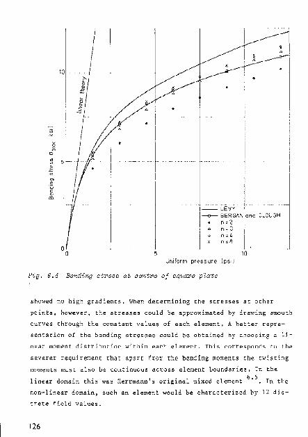
i I

__ LEVY I·· ---0-- BER GAN and CLDUGH

~,<

n ~ 3 ~d n.8

U~iform pressur~ [psi I

showed nO hif!;h gradients. When determining the stresses at other

points, however .. the stresses could be approximated by drawing smouth

curves through the constant values of each element. A hetter repre­

s~ntation of the bending ~tre85es cDuld be Dotained hy choo~in8 a li­

near mOTI:l~I"l.t distribution within eac.h element+ This corresponds tu the

severer reg\llrernent that apart fl;"om the bending moments the twisting

moments must also b" continuous aC):oss illement bound31""l.oils. In the

1 in€ar domain this Wa" Herrmann' s or iginal mix eo el ement 6.5 Tn tIle

non-linear domain, such an element would be characterized by 12 dis­

crete field values.

126

An additional improvement could be obtained by extending VISSER's

6.4 refined element to the non-l~near dorn~in. For this element, a

quadratic displacement aistribution has been chosen instead of a 11-

near one.

°bxx (ksil

10

5

0

O"bxx ( ksi)

10

5

a 2 4 6 8 y (in)

n",8

°O~--~----~~--~6----~ y (in,)

F(g. 6.5 Bending stre8se8 at x=O

127

The numerical computations for the plate were pe);"{onned by means

of a BURROUGHS B6700 eompt,1te~. T~ble III presents the computer time

requirements.

Table Ill, Computer time requirenlenta

.•. Element Time

modd min/~ec

n=2 6/56

n=3 22139

n=8 228/26

118

Summary and conclusions

Procedu.es ~o. the appro~imate ~nalysis of geometrica~~y non­

linear banding of plana baams and thin plates by means of mixed­

type finite elements are presented.

The mi~ed fo~ulation as introduced by Herrmann for the linear

domain has some distinct advantages over the customary displacement

formulation becauSe

(a) it is eaSy to formulate consistent elementS by usinS simple

approximating fUn¢tionsi

(b) both the displacements and the bending moments, being the most

important quantitie~ in a bending analy~i5. are the primary

variables o( the formulation. In the displacement formulation,

the bending mo~ents arC related to the second derivates of the

approximated deflections.

Owing to these advantages the possibility of extending the mixed

formulation to the geometrically non-linear domain has been explored.

It was ~xp~cted that this wDuld result in a u5efu~ ~inite-element

formulctt.ion.

The extension of the continuous variation~l formulation, the

applica~ion to f~n~te-element models, the solution procedures for the

pertinent non-linear equations, the computer programs as well as ~Ome

numerical examples are presented.

The procedures have been applied to the small-strain large-dis­

placement analysis of plane beams and to the von Karm~n finite de­

flection analysis of plates with arbitrary shape> arbitrary boundary

conditions and arbitrary loads.

Buckling analysis, althou~h expected to be possible with the

presented finite~element formulation, has not been considered.

129

I. The ~Dnclu~ions regarding the extension of the mixed fDrmulation

are:

1.1 Por the case of 1~r8e diaplacem~nts o~ plane beams and ffnite

deflections of plates, Herrm~nn'5 mixed variaeion~l principle

C$n effe~tively be extended to the seometric~lly nDn-linear

domain,

1.2 A BYBtematic procedure has been dev~loped to realize such ex­

t,O\nslon. The procedure stares from the geometrically non-t inear

potentiat energy formulation, The starting fO~rnu,ation must be

suQh th~t two systems can be di5ting~ished: the force-di.place­

ment system and the moment-rotation system. This can be effect­

ed by tempor~ry introduction o~ the 5hea~ deformation. The

first: ijy~tem is not tranBform~d. The second is transformed in

its complementary formulation: by applying Friedrich's t~ans­

fOTmatioTI, the rotations are replaced by mom~nts.

2. The following concluding remarks can be made in connection with

the appli~ation to plane heam problema;

130

2.1 For the beam, the S[a~t~ng potential energy fOrmllh.tion was

obtained by applying the well-known !"~3umption3 of ;beam theory

to the gener$l nOn-linear elasticity formulation.

2.2 The derived Herrmann formulation has been u~ed to constru~t a

mix"d finite-ele.ment formulation, the approach using CODrdinate

3yRtem~ moving with the eleme.nts, and known from displacem"nt

formulations, can also be util~z"d in the miXed large-displace­

ment fcrmul~tiQn+

2.3 !his change in coordinat" system make~ possible simplifications

in the element description if the element i~ taken S\,ffic.iently

small. Simple lo~al approximating functions can then be chosen.

2.4 The simplest beam element con3istertt with the requirements of

continuity of displacements I>nd moments has been develDped, The

d~5pla<:ements correspond to a ,igJd body lllovement together with

a I)nifQrm axial stHd.n. The bf:nding moment vad.es linearly in

the eleme~t. The element is characterized by 6 discrete field

val,ues+

2.5 A computer program utilizing this element has been ~eveloped.

Optimization of the prOgram ~aS not aime~ at. Unbranched plane

beam structures can be ~nalyzed, External moments at inter­

mediate nodes are not practicable. The examples presente~ in

Section 3.6 indicate that good results are to be expected with

programs baSed o~ the mixed finite-element approach.

3. In connection with the application ~o pLate bending we would

remark:

3,1 rhe derived He~rrnann formulation is based On the VOn Karman

theory which applies to de£lections up to 3 times the plate

thickness. The SUCCeSS of the effective extension of the mixed

formulation to this domain is attributable to the restrictions

of the von Karman theory. Moving coordinate systems are not

neede~.

3,2 The simplest triangular finite element consistent with the

requirements of continuity of the displacements and the bending

mom~nts (but not of th~ twi~ting momen~6) h?s been devehoped.

Th~ displac~m~nts are approximated by linear functions of the

fixed coo~~inates an~ the mom~nts by con~tant •. Th~ ~l~ment i.

characterized by 12 ~iscrete field values.

3.3 A computer program, utilizing tnis element has been developed,

Initially flat plates naving an arbit.rary shape and arbitrary

boundary conditions can be analyzed, The shape of the plate

must be approximated by a polygon. Generalized quantities must

be computed externally. Prescribed moments or rotatiOns are

only admitted at the bound~ry of the plate, Ihe ex?mple pre­

sented in Section 6,4 indicates that good results can be ob­

tained with thie appro?ch.

4. A deficiency of the extended mixed formulation is the lack of a

theory providing the criteria that must be respected in order that

131

Unite-element mooeJ.s witl1 an incr",a~ing number of elements con­

ver,ge to the cor~ect soll,lUon, Kno-.m critet"ia of the linear for­

mulation were respect",d, In out" examples, convergence was ob­

tained, With few elements the. a~~rcae.h underestimeted the ~tiff­

ness,

5, The seta of non-linear equations generated by the finite-element

models can eff",cti~ely be solved by II stepwise pt"ocedure, ~ach

step includeR a Newton-Raphson iteration on the previous results.

After each step, Newton-Raphson iteration can take place at the

option of th-e user+ In ,:iJl example~~ convergence of the iteration

prOcess was obQerved.

6. The following recommendations can be wade for improvin~ and eX­

tending the approach:

6.l In view of the large amount of compllting tim .. involved, opti­

mi"ation of the COmpl,lt .. r pro~ram and the solution strategy is

recommended.

The following subjects might be inve~tigated:

- determining the optimum solution strategy concerning (a) the

in~rem .. ntation of the independent and specified quantities

(number and sizes of steps), (b) when iteration shoulo be

performed and (c) the use of oV .. r- or under-r~laxation in

the iteration cycles;

- the possibihity of not adapting the system's matrices during

some iteration cycles;

- imprOVement of some algorithms of the progT8m.

6.2 Since for tile in-plane displacements as well as for the de­

flections of the plate the same local approximating functions

ar-e used, the program can be extended [or the analysis of

folded plate structures.

6,3 With the chosen approximating functions the stresses are con­

stant throughout the clement. The representation of the b .. nding

stresses could he improved by choosing a linear moment distri-

132

bution w~thin each el~mentt Thi~ corresponds to the severer

requirement that apart from the bending moments the twisting

moment~ must at~o be continuous. The representation of the mem­

brane stresses cDuld be improved by choosins quadratic instead

of linear displacement distributions. This refined element

would be characterized by 27 discrete field values.

6.4 The prc*rams could be extend~d to mak~ possible the analysis

of non-linear as well as linearized bucklin*.

133

APPENDIX A

Equations of the fini te displacement theo-.;y of eh$tici tl

Cartesian coordinates xi' together with a La~rangian description

will he used. Let Xi be the coordinates of ~ material point of a

body before deformation and let r be the position vector of that point

wi. til reference to the origin-

r = X,e. 1-1

(AI)

where ~i are •.• ni t ve"-tor~ along the fiKed axis.

Let .:..+!:. be the position vec.tor uf the same ffi8texial point after defor­

mation, where!:!. is the displac.eme.nt vec.tor:

(A2l

An infinitesiffial r~ctangular p~rallelepiped with edge Vect0rS !,i dXi =

~i dXi

in the undeformed state i~ deformed into a parallelepiped which

in Beneral is not rectangular. Its edge vectors are (r+u) _ dX. - - I~ 1

C(lmpo l1ents of

vec.tors !'. by -1

2e .. 1J

(lr:

e .. 1J

134

finite strain e .. may be defjneo 1J

meanS o[ the rdation

= .&i ''[j - 0-- Bi j - " - -1.1

I

2 (u. . +u - -+u . u . )

l.d J,~ rn:l'~ m t ]

1J

(1\3)

in te.rm!;l of the latrice

(M)

(A5)

dS 2

~2

dX2

!1 l\1

Fig. Al Two-dimensional representation of stress

The relation between these components of strain and the engineering

strains Ei and ~ij (~i being the elongation of line element dX i and

~ij the change of the angle betw~en line elements dX i and dX j ) can be

obtained by comp~ring the lengths of the deformed and the undeformed

sides:

ds. dX~ = l+gi = lail,

l.

and by denoting the new angle between the sides

follows from (A4) that

k I • ~ rg:-:g:' = Ji+2;:-:' ~1 " E..i '.E.i"" u.

(A6)

and .!!. - I 2 l/! ij" t

(A7)

135

while

.a1, 'i

J' W Ig, 111l..I<;:os(~ - 'iJ •. )

-1 J " 1J

The relations are then:

~. =_I~-l l." 11 (A9)

(AIO)

Let s_ be the. rOT.<:e pe.r unit undeformed ;;t:rea~ acting on an ~lement of -.)

a~ea which befor~ deformation was perpendicular to e .• According to -J

KAPPUS'compon~nts of (pseudo) stress are defined by writing

(All)

Ten~or ~ jk is commonly named the (symmetric) Piola~Kir"hhoff stress

ten~or. The ulagni tudes of the s tress components are:

(AI :n

Irtrroduction of (A3) and (All) into the force equilibrium equation:

!j,j+!=O, where f is the force per unit unde[ormed vo<ume, le3ds to

the following three scalar equilibrium equations:

(AI])

'l'he c.onditiono of moment equilibrium for the defQrm~d parallelepiped

are of the form;

s . kJ

(AI4)

The system of differential equations (A'), (AI]) and (AI4) 18 completed

136

by the stress-strain relations, which for linear, elastic and isotropic

material have the form:

S •• 'J

(A1S)

For the formulation of bounaary conditions we require a component re­

presentation of surface forces. Let Pm be the xm-component of surface

force per unit unaeformed area acting on an element of area which

b~fore aeformation was perpendicular to a vecto~ ~, with components

nj

. The condition of fcrce equilibrium for an infinitesimal tetra­

hedron with sides perpendicular to n and ~i before defo~mation gives

(AI6)

~) Kappus, R.: zur Elastizitatstheorie endlicher Verschiebungen, Zeit­

schrift fur an~ewandte Mathematik und Mechanik, 19 (Oct. and Dec.

1939), p.271-285 and p.344~361.

137

APPE.NDIX B

Numerical solution of sets of non-linear equations

A method as descrihed hy STRICKLIN and HAISL£l(' 1B used, whi"h

cOns is ts of an i.n~remef\tal apprO.f.l.ch V3r ied by Newton-Raphson i t.~rB t ion I

To descrihe the method. let us consider the sy~tem of n non-linear

equations in the unknowns '11''12' .... • .'1n'

fl(ql .'12 '" ····qn) ~ QI

~2(ql·q2·""· ,qn) 92 fn ('II ,Q2' ..... ,'In) On

where Q1'QZ' .... ,Qn

are given constants.

We can Blso write (81) in the concise form

f(q) - <l o

(DI)

(B2)

where f is the vector with components f_ of (BI), q is the vector 1

with unknowns qi and Q the vector with constants Qi' Since pure itera-

tion of (B2) converges only for special cases, and the objective of a

non-lineal: analysis is usually more than to find a single solution

(e,g, the deformation history), " parameter p is introduced

o ~ p s (BJ)

1l.nd the solutions q=q(p), PL[a,l] are gO determined that

f(q) - pQ o (SI! )

138

We nOw assum~ that

(I) a solution q=q(p) exists for each pe[a, I] ,

(2) q(p) is continuously ~iftel"entiable with respect to p. and

(3) f(q) hs~ ~ontinuous partial derivatives with respect to all

components "i'

Then, if q is a solution of (B4) corresponding to p and q+~q a solu­

tion corresponding to p+6p

f(q+~q) - (p+6p)Q ~ a (85)

From the assumed differentiabi,ity of f, we have. to within lin@ar

terms in ~q,

f(q+.:).q) feq) + J(,,)tlq (B6)

where we have the matrix

J(q) n [3f-CQ)/aq.] 1 J Q

(Rn

If J is non-singular, 6q can be determined from (B5). Since q was a

solution corresponding to p this gives

-I 6q = J (q) Ap Q (BB)

This leads directly to an incremental numerical method fDr solving

(BI) :

Let PE::[O,IJ ,q(O) = a and J(q) be non-singular for all p under con­

sideration. Divide the interval [0, IJ into M partitions

(119)

(B10)

139

(BII)

Then a path q=q(p) could be generated by the following process

(r) q

(r-I) (r) q +Lq (BI2)

(BI3)

HOwever, ~orne error will inevitably ~nt~r each step of the process

becauSe aPr i. finite and the Taylor expansion has b~en restricted

to the linear term. According to Stricklin and Haisler, the error

can be effectively ~educed by observing that q(t) ia not the exact

solution of (&4), corresponding to Q(r) and thus f(q(r))_Q(r) is not

exactly 2(lrO and may not be omitted from (6) .her applying the

Taylor e"pan~ion, instead of (513) we then have

(flI4)

A way of still further improving the accuracy of q(r) at a certain (rl , (r)

value Q ,a to uae q generated by (BI2) and (BI3) as a trial

solution eor initiating Newton-RaphBon iteration, The Newton-Raphson

m~thod 8eek~ a correction 6Q(r,m+l) on a trial solution q(r,m) ob­

tained a£te~ r stQpa and m iterate~, such chat f(q) - pQ vanishes,

o (1l1.5)

Again applying a first order Taylor expansion ,n (BIS) giv~s

(BI6)

and the correction llq(r,m+l) c(>n be obtained from

(B 17)

140

where Q(r) _ f(q(r.m»is the residue. The improved sot~t~on

(.,lIl+lj (r,J!\) (r,m+l) q m q + ~q (BI8)

can be ~eed as a new trial solution and the process is repeated ~ntil

a euffieient degree of acc~raey has been obtained.

COlllparison of (BI7) with (BI4) shows that both expressions are

nearly identical. The incremental eq~ation contains ~Q(r). which term

i5 absent in (BI8). In view of (BI7), the extension of the increlllen­

tal equation can b~ interpreted as a Wewton-Raphson correction.

·Stricklin, J.A., Haisler, W.E.: G~oJ!\etrical non-linear gtr~ct~ral

analysis by the direct stiffness method. r.oc. of the Symp. lUTAN,

Liege, 1970. (High speed computing of elastic str~ctures).

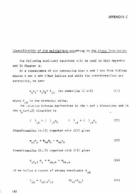
APPENDIX C

Identification of the multipliers occurring in thCJC)ate formulation

The following auxiliary equations will be uSed in this Appecndix

and in Ch~pter 4:

As a consequence of our convention that a and e are fr~e indices

wheras nand s are fixed indices and while the transformations ar~

,eve,sible, we have

eel)

where 8~B i8 the Kronecker delta.

The relBtiort b~tween derivatives 1n the nand s directiOn~ and in

) ,n

) n ,It CI. s ,

'fransformation (4.13) toge.ther with (el) gives

Transformation (4.13) together with (C2) gives

m + m l'ln,.n nStB

If We define a t~nsor of stress resultants N as

142

(r.2)

(C3)

(C4)

(es)

chis cransforms according to

N

Analogously to (G3) we hsve

ss N s g

I;(S C. S

(C6)

(el)

Now we consider the potential energy functional (4.23) and remove the

constr"tnts

~(l = w in A (4.3) ,<>

~ a W- and <fis a ..- on 5 (4.5) n ,Ii ,s

I in "c.S

~ 2{~C.,S+.pS,c.) A (4.15)

¢ -n ° 1>n on S<j> (4.21 )

by introducing them into the functtonal by ~e~ns of che overbarred - - - -

multipliers Q • Unn ' Mns' mc.S and MIin .espectively

u -{ [.!.. A K ( +.!.. E ~ ~ _ 0", + I A 2 c.sy6 c.S ye 2 c.Sye I;(B yo q

.;;; to: .1.($ +¢ )t. Q ($_..- )JdA+ ('<6 c.6 2 c., S S, c>. f c. <;I. ,'"

.f Vow ds -1 mO ¢ ds -{ pou ds .f M ($ -¢O)ds + Js n S Iin n S c. c. J s nn n Ii

V m p $

+f ~ (4) -W )ds -fM (~-w )ds - ""pO. W _ (C8) nn n , n ns a , S L..J Z J .1

j

We suppOse the pultiplie.g m"'6 Co be symmetric and to transform simi-

l arly to m~R (4,13), while Qa lS ~uppo~cd to transform similarly to

Q(i (4,12)

T(!enti.fi.cat~ot\ of ti1" mUltipliers proceeds (IS follQws: We requir~ U 1

to b~ stationary with respect to variations of K, wand ¢:

where

6 \II 0 =f[A .~ - OO,,(1J6<a,; (lA «(;9) ': A c.0yli y"

6 III - 0 =j~[Ea~Y6f.Y60W'''3 -0

+ Q 6w }A + (C Ill) q 6w w 0:. '1:1

+£ M 6w as - L pO .ow. JPs nS ,5 . ZJ J .J

Q 6¢ JdA {mO 64 ds +

~" S nn n 6. U

J = 0 =J [;;; !(6~ +6~ )-

,. A ~f2 a,e e;o

-f M O¢ ds+l~ o¢ ds-r[M ~~. ds(CI1) S nn n J~ nn n J; nS s

1,

(CI2.)

The stationary condition of (C9) is

In A (eI3)

Formulation of the stationary condition of (CI(l) with subsidiary con­

dition (CI2) is more laborious

We introduce the stress resultants NoSCCS) into th~ first term of

(CIO)

W" write

f[N W + Q ]ow dA ~£[N W + Q In. 0W ds ~ A ~S ,8 ~ ~a J~ ~B ,6 a ~

-rrN W + Q J liw ds J A .. ,,6,B I) ,0' (eI5)

1M

white in view of (C7) and (e2) we have

J N Sn w 00"d5 =1: eN w + N w ) 6w ds J's 0. (l ,0 J's nn ,n ns, s (CI6)

The termj( M OW ds must be retained in (CIO) beca~se the conei-Y'.. ns ."s nuity of Mns is unknown while we allow the edg~ of the plate to have

angular points whieh, if occu~ring, cause w to be discontinuous. ,~

Since ow is not an independant variation, we must write , s

f M ow d~ S ns ,8

[ M ow] -j( M oW ds ns s J's ns,s

(CIl)

where [M OW], indicat~s that a~< p06sible discontinuiti~s of M m S M must be taken into ~ccount.

Introduction of (CI4),(CIS),(CI6) and (CI7) into (CIO) giv~s th~

following stationary conditions

(0 +N SW s) + 0

= 0 A (CI8) q 1n a i]. 10 1[;(.

~nn 0 on S (CI9)

fin + N w + N w - M Vo on Sv (e20) nn ,n nS ,5 ns"s n

i1(-) Me+) 0 point~ (C21) p . ",t

uS ns Z]

where MC-) is the value of M when approaching point j if we proceed nS ns _(+)

in the s direction, while the value is Mns when w~ l~aVe point j.

The sta~ionary conditions of (CII) can be obtained by ueing the

assumed symme~ry of m~$ in the first term,

1 1 -- m (6~ +6~ ) dA =

A 2 0.8 ~,$ $,~

I iii ,6¢ no ds -J;;; 0 o6¢ dA )Vs ~o a, A ~o,o 0. (e22)

HS

since the pultipliera ma~ transform according to (4.13)

f iii G n ,,6¢ os =,[ iii 6~ ds +1.;;; 6,p do S a"" a J~ nn n S nS 5

(C23)

The stationary conditions of (Gil) are then ~

m aR,R

+ Q(l = 0 in A (C24)

+ 0

6 m ,I 1\1 on nn nn nn In

(C25)

m + ,I lin nn

- M 0 nn on (C26)

rn - M = 0 on S ns ns

(C27)

A comparison of all st3tionary conditions thus obtained with the

governing equations 4.3 enables U8 to identify the pultipliere'

Bq.(C13) corresponds to the constitutive equations

Eq.(CJ8) corresponds to th~ equation expressing equilibrium 1n the

"3 direction.

Eg. (C20) c.orresponds to the equation which coupl~s so-called

effective shear force to the transverse edge load.

- Eq. (C21) corr-esponcis to the equation expreSSlng the. discont.in~d.ty

of twist1ng moroetlt~ CU3Sed by ti uonLenttated trtinsverse force.

- Eg.(C24) co~respond" to the equation .xpre8sing equilihrium of

moments.

- Eq.(C25) couples m to the prescribed normal moment mO nn nn

Thus, the multipliers can be identified as follows

m <"\ ~~

= rn o:B

in A «(28)

Q = Q in A (C29) C1 "

M m on S (00) ns I'l.S

M = m on S (C31) nn nn

146

APPENDIX D

Auxiliary relations ~eeerred to in Ghapter 5.

In view of (5.40) and (5.41) we have

(DI)

sin~e fl~8v v (5.31) are the in-plane strains if there is no defl@c­

tion, it is justifiab.e to introduce the membrane £orce~:

(D2)

Since Bwl -6 14 w' using definition (5.32a) for ~l' together with Eq. (D2),

we ~an write for part wT 6~l Dll Bv v of (Dl)

[

a", w N W

- x ax a1'",w

N -­xy ax

o

~ [N N] [L] <j> <if x xy oX "

N N L l(Y Y ay

(D3)

147

If we introduce the matri~,

Q = [N N 1 o x xy

N N xy y

(n4)

and use definition (S.32b) for liZ together with the eJ<pressl on 11 2¢,.w=

Bw2,. (5.35), we obtain for (D2)

(D5)

Combining (01) and (05) gives'

T k( I) T 't B '01 = wI k C)) w v w Bw2 °0 w wv w2 ww

Since °0 is symmetric., the matrix k (1) is symmetric. ww

The virtual work equmrion is obtained by taking the first variation

of (5.62) and taking into account th~t some component matrices are func­

tions of displacem~nts. Ihe resulting expreSSion mu?t be gO transformed

that component matrices without variations appear, e.g.

(D7)

The following auxiliary relations can oe u?ed:

Referdng to the ddinitions of W (5.3)), Bwl and llw2 (5. )5) i,t <:a,\

be proved th~t;

(I)S)

Ihis relation, together with the definitions .of k(l) (5.40) and k(2) vw ww

(5.42), gives:

148

6k (l)", k(l) 6" vw vw

(D9)

6k (2\, 2 k(2) 0W ww ww

(DID)

Moreover, l,lsing (D6) it follows th?t

ok (I)", k (I) ww wv

6v (DI I)

UBing th~~e auxiliary rel~tione, together with the ~~~try pro­

p~rti~s k(l) = k(l) and (k(2))T k(2) the symm~tric expr~ssion wv V"W ww W'W' ,.

(5.69) will be obtained.

The stationary condition for a confirguration th~t i5 c105e to

the configu~ation ctescrib@d by (5.69) can be obtain~d by replacing

v by v+<lv, W by w+ llw, and m by Ill+<llll. The im:rementa1 equation is

then obtained by taking the differ~n~e b~tween the two configurations

and r~taining terms which ~re linear in the inc~ernents. e.g.

Again, the increments are expelled from the component matrices. Ana­

logously to (08) W~ have

(DI3)

50 that

(DI4)

The other al,lxili~ry relations can be obtained by l,lsing (D9), DIG) and

(DII) and replacing Q by A.

149

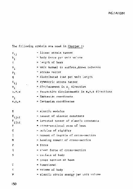
NOTATION

Th~ following symbols are used in Chapter I:

e - , LJ

k. 1

n. 1

Pi q

t .. L.[

U. L

UtVtw'

E

Eijk~

F ijU F

G

M

r Q

u V

W

ISO

lin~ar ~train tensor

body force per unit volume

length of beam

unit normal to ~urface7drawn ovtwsrds

stres,;; "~cto:r

~ distributed load per unit length

= symmetric stress tensor

displacement in xi direction

~ respective displaceillent~ in x,y,~ directions

Cartesian coordinate

Cartesian coordinates

el"sd c modulus

~ tensOL of eldstic constants

- iTIvert~d tensor of elastic constants

• cross-sectional a~ea of beam

= modulus of rigidity

moment of inertia of Cr05S-BectiOn

bending moment of cross-section

~hear foree of cross-section

surf"c" Df bDdy

cross-~ection of heam

= functional

= volume of body

elastic strain energy per uldt volllme

superscripts;

o

subscripts:

i,j,k,~

c

CIL shea.r strain

~ variation symbol

.. bending str~irt

~ ~ot~tion of cross-section

c specified quantities

Cart~6iart components

~ compl~mentary

In Chapter 2 the followirtg symbols are u.ed additionally or they have

a differ~nt meaning:

e e - components o~ the nOn-lirt~~r strain tensor at poirtts xx' xy"'"''''

exx.,exy"ll""·'

Sxx;Sxy,·· .. · .

u,v,w

N

X,Y,Z

YlIY,)'"Z

Yxy'Yxz

" x

of the axis of th~ beam

~ comportents of the non-linear strain tensor

~ components of the symmetric Piola-Kirchhoff stress

teneor

displacement. of points of the axis of the b~am in

x,y,z directions respectiv~ly

axial force of the cross-section

initial Cartesiart ~oordinates

angle between deformed axis of beam and x-aXLS

• shear deformations at points of the axis of the beam

shear deformatiort

true axial .trairt

mul tiplier

displaCements in x.y,z directiorts respectively

~ angle of shear in the X,z plarte

!S!

In Chapter .l the fOllowing symbol. are used additionally or they have

a diHe.rent meaning:

a

11

p

q

r

u,W

u,W

x,z

.. " x ,z

x,z

Q

s T

x,Z

" " x ,z

¢

superscripts: k

T

subscripts:

152

span of beam and plate

vector with non-linear functions

plate thickness

total numher of discrete field values

distributed transverse load per unit ~re~

vector with discrete field valu~s

"enor (3. :,11.)

global displacem~nt~ in X1Z directions respectively

local displacements in x, z directions respectively

fixed Cartesian global coordinates

initial local coordinates

c displaceo ~o~al coordinates vector with gene~alized loads and rotations

element matrix (3.32)

transformation matrix (3.33)

material coordinate~ with respect to the XtZ system

material coordinates with respect to the . x ,"

rigid body rotation of heam element in the K~~ pldI~~

~ relative accuracy

rotation of cro~5-section relative to the x,~ systelD

element number

transposed

= number of the discrete field value of tI,e element

number of the structural discrete field v~lue

The following symbols are used in Chapter 4:

h

A

L

- plate thicknes~

~ stress resultants Eq.(4.11)

outward normal to the ecge contour

in-pl~ne edge load per unit length

q t~ansver5~ pr~8~Ur~

- symmetric Piola-~irchhoff stress ten6~r

coordinate along plate boundary S

unit vector tangent to the edge c~ntour

~ in-plane displacements of points of the middle sur­

face

deflection of middle $urface

fixed Car~esi~n coordinate sy~t~m

region occupied by the middle surface of the undefor­

med plate

c tensor with local membrane stiffnesses, Egs.(4.16)

and (4.l8)

~ inv~rt~d tensor A

= tensor with local bending stiffnesses, Eqs. (4.17) and

(4.l9)

- typical plate dim~nsion

• total number of elements

stress resultants, Eq.(4.9)

E concentrated transverse fcrees

c s~res~ resultant (4,10)

- boundary of the middle surface of the plat~

- functional

~ edge shear loads per unit length

c initi~l CBLt~sian coordinaLe~

= variational symbol

~ components of the Gr~en's strain tensor in the middle

~urface of the plate, Eq. (4.14)

153

superscripts:

(l

subscripts:

n

("(,B,Y,"

angle between outward normal ~ and the xI axis

bend£ng and twisting 5train~. Bq. (4,15)

in-plane displacements

- small rotations of material lines which odginally

were straight and perpendicular to the mi';!.;!'e 6Ilrh.<;e

r element number

preBcribed

Cartesian components

indicates points j at the ~ontour

= normal direction

~ tangential direction

Carte~ian ~omponents in the plane of the plate

In Chapter 5 the following symbols are use.;! additionally or th"y

have a different meaning;

a. f~ £(0)

rom

length of element side i

vectOr with element nOn-linear equations

~ matri~ defined by Eq. (5.32)

k(o) ,k(l~k(l~k(2)= constitllents of element matrices, defJned Ily Eqs, VV vtJ '-7tJ 'YJ'W

(5.47), (5,48), (5,49) and (5.50)

matrix defined hy Eq. (5.74)

= matrix defined by Eq. (5.79)

= vector with discrete normal moment~ defined by ~q.

(5.21 )

= vector with Cartesian components of moments, define.;!

by Eq. (5.2Z)

qk a vector with element dis~rete field values, Eq. (5.92)

u(x,y),v(x,y) in-plane displacements

154

u~ ~v i v

w(x,y)

W. 1

w

F

G

GI

1. t

J. t

Kk I

P pO po po

V' WI m

T

W

= o~screCe in-plAne displa~em~nt~

• vector with in-plane discrete displacemen~s, Eq.

(5.15)

- d~flection of plate

discrete values of deflection

= vector with discrete deflections, Eq. (5.8)

in-plane Cartesian coordinate.

- Cartesian coordinates of angular points

element area

= matrix defined by Eq. (5.23)

• matrix d~fined by Eq. (5.42)

CI ma.rl"ix d~fined by Eqs. (5.43)

matrix defined by Eq. (5.45)

matrix defined by Eq. (5.71

matrix defined by Eq. (5.66)

and (5.44)

~ matrix with local membrane stiffnesses, defined by

Eq. (5.37)

~ matrix with local bending elexibilities defined by

Eq. (5.29)

I:i matrix defined by Eq. (5.62)

matrix defined by Eq. (5.60)

;;;; matrix defined by Eq. (5.48)

number of element anglllar point

number of node on sioe i

~ element incremental matrix, Eq. (5.99)

• matrix defined by Eq. (5.'2)

~ vectors with g~nerBlized in-plane for~~s, transverse

forces, and rotations ~espectively

vecto~ with generalized forces and rotations of the

elament, Eq. (5.93)

matrix defined by Eq. (5.10)

matr~x defined by Eq. (5.39)

155

x

'I' w

superscripts

(0)

(1)(2)

1<

subscripts

I

matrix d~fin~d by Eq. (5.6)

incrertlent

~ differential operators defined by Eq. (5,111))

vec.tor with linear parts of $train ten~Ol', Eq. (') . .3)d

~ vector with non~liDea~ part~ of strain tensor. Eq.

(5.35)

matrix defined by Eq. (5.77)

matrix with interpolating functions, ~qs. (5.11) .nd

(5.14)

- matrix with interpolatinR functions defined by Eq.

(5. 1$)

matrix with interpolating functions defined by Eq.

(5.38)

constclrtt

linear and qdadrat(c in discrete field values

number of element

side and angular-point numbers

incremental

In Chapter I; the following symbols are used addi tionally or they have

a differ~nt meaning.

kk qq k

k1qq

m

" m

156

non-1inear element matrix

~ increnlental elem~nt matrix

- vector with unknown normal moments of the eneir"

S true tl,lre

- vector witb _~pec.ifie.d normal rnOIYleI"l.ts of the entire

stru.;:.ture

q

o '1

1/

w

o w

vect~r with all unknown discrete field value. of the

entire structur@

vec~or with all sp@cifi@d di~crete field values of

the entire structure

= ve~tor with unknown in-plane displacements of the

entire structure

- vector with specified in-plane displacements of the

entire structure

ve~tor with unknown deflections of the entire struc-

tur@

~ vector with specified deflections of the entire

struct\,lre

K ,K ,K o,K 0 - non-linear system matrices with reference to the qq U\,l uu unl quantities denoted by the subscripts

Klqq,KI\,lu,KI\,l\,l°,KrumO= incremental system matri~es with reference to

the quantities denoted by the subs~ripts

KC]) ,K C]) KC])K C2 ) KCo)K(o) F(o) = component matrices of the non-vv vw' wv· 'WW ' wm' JIlW • Dlm

linear sys~em metrix K(l) K(l) K(l) K(l) K(2) K(ol K(o) p(o) _ component matrices of in-

Iv\' I rvw' lwv l Iww' Iww' Iwm." Imw ' Imtn

Q

cr~nlental system matrix

location matrix defined by Eq. (6.5)

~ vectors with unknown rotations, in-plane forces,

and transverse forces respectively

~ vector with specified rotations, in-plane fo~ce3,

and tran$Verse forces respectively

~ vector w~th specif~ed generalized forces and rota­

tions of the entire structure.

157

REFERENCES

Introduction:

I. Clough, R.W. ~nd Tochef, J .L. : Finite element stiffness f"(I~triceg

for analysis of plate bending. Proc. of th~ first conferenea on

matrix methods in ~truetural mechanics, AiT Flree Flight Dynamics

L~b., Technic.a] report 66-80, Wright P~tt~rson Air Force 113G~,

Dayton, Ohio, 1966, p. 515-545.

2. Ziertkiewicz, O.C.: The finice element method in structural and

continuum mechanics, Me Graw-Hi 11 , London, 1967.

J. Oliveirl', p .• R. de Ararttes e: The mathe[ll(lt;ical theory of structu­

res, NATO Advanced Study JnstiCvte on finite el~ment meth"d. in

continuum mechanics, Lisbon, 197).

4, BazeleytG.R.,Cheurtg, Y.K., IronS I B.M., zienkiewicz~ OfC,I Trian­

gulaf elem,;,nts in plate. b~nding. COnforming and non-conforming

solutions. Proe. of the first cortference gn matrix method" in

structvra 1 mechanics, Air Porc~ FI ighe Dynamics Lab., T"chni.~.al

repo>:t 66-BD, Wright Patterson Air Force Base, DaytOn, Ohio, I,nc,.

5. Bell, K.: An~lY515 oE thin plat~s in bending u,ing triangular

finite ~lcm~nts. lnstitut for Scatik, Norges Tekniske H~gskol~,

Trondheim, 1968.

6. Vi~.er, W.: The finite element method in deformation and heat Con­

duct ion probl"!lls. Illes is, DeIf t, 1968.

7. Hsieh,'f.K., Clough, R.W., Tocher, J.L.: I'inite element;: stiffness

matrices for analysis of plates in be.ndinll' Prot. of the fir.H

1.58

~onfe~ence on matrix method. in structural me~hanic5, Air Force

Fli~ht Dynamics Lab., Technical report 66-80, wright Patterson

A~r Force Base, Dayton, Ohio, 1966.

8. Clough, R.W., Felippa, C.A.: A refined quadrilat~ral element for

analysis of plate bending. Proe. of the second conference on ma­

tr~x methods in structura~ mechanics, Air Force flight Dynamics

Lab., Technical report 68-150, Dayton, Ohio, 19&8, p. 399-440.

9. Eer~an, P.G., Clo~gh, R.W.: Large deflection analys i5 of plates

and shallow shells using the finite ~lement method. International

Journal for N~merical Methods in Engineerin&, Vol.5(1973),

p. 543-556.

10. Oden, J.T.: Theory of conjugat~ projections in finite element

analysis. NATO Advanced Study Institute on finite el~mcnt methods

in continuum mechanics, Lisbon, 1971.

II. Herrmann, L.R.: A bending analysis for plates, Proe, of the first

conference on ~trix methods in structural mechanics, Air Force

Flight Dynamic~ Lab., Technical report 66-80, Wright Patterson

Air Force Base, Dayton, Ohio, 1966, p. 577-604.

12. ~errmann, L.R.: Finite element bending analysis for plateB, Jour­

nal of th~ Engineering Mechanics Division, Proceedin&e of the

American Society of Civil En&ine~rs, Vol. 93 (1967). p. 13-26.

13. Turner, M.J,. et al: Large deflection analysis of complex struc­

tures s~bjected to heating and external loads, Joural of Aero/

Space Sciences, Vol,27 (1960).

14. Gallagher, R.H., et a1: A discrete element procedure for thin

~hell instability analysis, AIAA Journal, Vol. 5 (1967), No. I,

p, 138-145.

159

15. Mall~t, R.H., Mar9a<, P.V.: Finite element analysis of non­

lin~ar stru~tur~s, Journal of the Structural Division, froe. of

the American Society of civil Engineers, Vol.94 (196S), No.ST9,

p. 2081-2105.

16. Kappus, R.: Zur t:lastizitatstheorie endlicher Verschiebung~n,

Zeitsch>:Ut fu{" (lngewandte Mathematik und Meehan!.l', 19 (Oct.

:;>.nd Dec. 19:39), p. 271-285 and p. 344-361.

17. Reissn"r, E.: On a variational th"or"m in elasticity, J. Matb.

and Phys., 29 (1950), p. 90-95,

18. Reissne>:, E.: On a variational theorem for fini te elastic defor­

mations, J. Math. and Phys., 23 (1953), no.2-:J.

19. TOnti', E.: Variational principles irt ela.tostatics, Meccanica,

Dec. 1967, p. 201-208.

20. Tereg!Jlov, I.G.: On :;>. vad.at~on .. l theorem of the non-Linear

theory of elasticity, J. Appl. Math. and Mech" USSR, Vol.26 (19~2)

p. 234-237.

21. Zubov, L.M. : The 6tationary prin~ipl" of complerocI~ta1:'Y worl, in

non-linear theory 0[ elasti.::ity,Prikl. Mat. M.;,kh., Vol. 34 (19'10),

p. 241-245, En~lish translation 228-232.

22. Kaiter, W.T.; On the prirtcipla of stationary complementary energy

in the non-linear theory of elasticity, Report no, 488, Jartuari

1973, Laboratory of Engineering Mechanics, Delft University uf

Technology.

23. Washizu, K.: variational methods in elBsticity and plasticity,

Oxford, Pergamon, 1968.

160

Chapter 1

I. washizu,K.: Variational methods in elasticity and plast~city,

Oxford, PerSamOn, 1968.

2. Herrmann, L.R.: A Bending Analysis for Plates, A.F.F.D.L.-TR-66-80,

Froceedings, Conference on Matrix Methods in Structural Mechanics,

Wright-Patterson Air Force Base, Ohio, 1965, pp. 577-604.

Chapter 2

2.1 Kappus, R.: Zur Elastizitatstheorie endlicher Verschiebungen,

Zeitschrift fur angewandte Mathematik und Mechanik, 19 (Oct.and

D~c.1939), p.271-285 and p.344-361.

2.2 Fung, Y.C.! Foundations of solid mechanics, Prenticehall, Inc.

Englewood Cliffs, New Jersey, 1965.

2.3 Zubov, L.M.: The stationary principle of complementary work in

non-linear theory of e'6stic ity, Prikl.Mat.Mekh., Vol.34 (1970),

p.241-24S, English translation p.228-23Z.

2.4 Koiter, W.T.: On the principle of stationary complementary energy

in the nOn-linear theory of elasticity, Report no.488, January

1973, Laboratory of Engineering MeChanics, Delrt University of

Technology.

Chapter

3.1 Courant, R., and Hilbert, D.: Methods of mathematical physics.

Vol. I, lnteraeience, New York, 1953.

3.2 Oliveira, E.R., d~ Arantes e; The mathematical theory of structures,

NATO Advanced Study Institute on finite element methods in continuuw

mechanics, Lisbon, 1971.

161

3.3 Brebbia, C., Connor, J.: Geometrically nonlin~ar finit~-el~ment

analysis. Journal of the Engineerin~ Mechanics Diviaion~ Proc. of

the American Society of Civil Engineers, Vol. 9~ (1969), p. 40J-

4S.1.

3.4 Bergan, P.G., Clough. R.W.: Large deflection analysis of plates

and shallow sh.;,ll~ u~ing the finite demen!; metl,od. Inte);"national

Journal for Numerical Method. in Engineering. Vol. 5 (1973). p.543-

556.

3.5 Murray, D.W., WilBon, E.L.: Fin~ce elc)~ent large deflection analysis

of places, Journal of the Engineering Mechanics Divi,ion, froc. of

the American Society of Civil Engineers, Vol. 95 (1969). p.li!3-16;'.

3,6 Besseling, J.F,: Non-linear probl",m~; Course On numerical a.nalysi!;

of .tresses and vibration~, held at the Department of Mechanicsl

En8inee~ing of the Delft Univ~r8ity of Technology, Delft, 19h!.

3.7 Fung, Y.c,: Foundations of solid mechaoics. Prentice-hall, Inc.

BnglewoDd Cliffs, Ne~ Jersey. 1965.

3.8 Menken. C.M.: Large deflection analysis of heams with mixed finite

elements, Report WE, Eindhoven, University of 'fechno].<J8Y (to be

published) .

3.9 Yang, T.Y.: Finite displacement plate flexure by use of matri" in­

cr~mental approach. Tnternational Journal ~or Numerical Methods in

Engineering, Vol, 4 (1972), p.4IS-432.

Chapter 4

4.1 Bergan, F,G., Clough, R.W.: Large deflection snalysJ.s o[ plate"

and shallow shells using the finite element method. International,

Journal for Nul'ller ical Methods in F.nB).need.ng. Vol. 5 (]973), p.

543-556.

162

4.2 Fung, Y.C.: Foundations of solid mechanics, Prentice-hall, Inc.,

Englewood Cliffs, New Jersey, 1965.

4.3 Washizu, K.: V~ri~t~on~l method~ ~n ela$ti~icy and plasci~icy,

Pergamon Prees, 1~68.

4.4 Herrmann, L.R.: A bending analysis for plates, Proe. of the first

conference on matrix methods in structural mechanica, Air Force

Flight Dynamics Lab., T~chnical r~port 66-80, Wright Patt~rson Air

Force B~se, Dayton, Ohio, 1966, p.S77-604.

4,5 Herrmann, L.R., FiniCe element bending analysis for plates, Journal

of the Engineering Mechanics Division, Proceedings of the ~erican

Society of Civil Engineers, Vol. 93 (1967), p.23-26.

Chapter 5

5.1 Bargan, P,G., Clough, R.W.: Large deflection analysis of plates

and shallow shells using the finite element method. International

Journal for Numerical Methods in Engineering, Vol. 5 (1973), p,

543-556.

5.2 Mallet, R.H., Mar~al, P.V.: Finite element analysis of nonlinear

structures. Journal of the Structural Division, P,Qceed~ng3 Qf the

American Society of C~vil Engineers, Vol. 94 (1968), No. ST 9.

p.2081-2105.

Chapter 6

6.1 Vieeer, w.! The finite element method in deformation and heat

conduction problem~, Doctoral Theei~, Techn. Un. Delft, March

1968.

163

6.2 Bergan, P.C., Clough, R,W,' Large deflaction analysis of p18t~s

and shallow "hells using r.he finite element method, Lnternatio­

nal Jou<nal for Numerical Methods in Engineering, Vol., 5 (1973),

p. 543-556

6.3 TimoshcnKo, s,P" Woinowski-KriegeJ", S.: Theory of plates 8nd

shells. Second edition, McGraw-Hill, New York, foronto, London,

1959

6.1, Visser, w,' A refi.ned mixed~type plate bending element. AIM.

Journ~l, Vol. 7, No,9 (1969), pp. 1801-1803.

6.5 He<rmann. L.K.: A bending analysis for plateR, A.f.F.D.L.-TR-

66-80, Proceeding" Conference on Matrix Mech6dR in Structural

Mechanics, Wright-Patterson Air Force Base, Ohio, 1965, pp.

577-604

164

STELLINGEN

1. Ret door Herrmann voor lineaire buigproblemen gefo1;"muleerde

variatieprincipe kan op ~stematiSche wij~e worden uitgebreid tot

geom£tri~ch niet-lineaire buigprQblemen. De elementenmethode geba­

Seerd op die ui~gebreide principe vormc een praceisch bruikbaar

sereedschap voor het construeren van benaderingsoploaaingen.

Herrmann, L.R.: A bending snalysis for plates. Proc. of

the fir~t conference on matrix ~thods in structural mecha­

nics. Air Force Flight Dynamics Lab" Techni~al Report

66~80, Wright Patterson Air Force Base, Dayton, Ohio, 1966

p. 577-604.

2. Het is onjuist het variatiepTincip~ van Herrmann op t~ vat ten

als een uitwerkin~ van het prancipe van Reissne~.

Cook, R.D.: Eisenvalu£ problems with a ~i~ed pl~te element.

AlAA Journal, vol.7, no.5, may 1969, p.96Z-963.

:Blauwend-raad'llJ "': Pormalisms en inzicht in mechanics modelle.n.

R'jk.wate'.taat-.e~ie 13, Bept.1973, p.llO.

~r Aet formuleren van variatieprincipes in de technische mechanica

door~

- uit te gaan van de geldende relaties~

- .lk. r.latie to vermenigvuldigBn mBt eon wi""Bkeu.~ge funot~c

waaraan later een betekenis woret toegekend,

- elk zo verkregen product on~er te brengen in ecn integraal

ove. het geld~gheidsgcbied van de bBtrBffende rBlatie,

- te Stellen dat de 80m van dBze integrale", -,'ul moel: ti.jn.

moet om i~zi~htel~jt~ redenen W01:den ~f8er~en.

Blauwendraad. J,: FQrmalisme en in.icht in mechanica ~dellBn

RijkBwaterBtaat-BBriB 13, ~BPt. 1973, p.IIO.

~. De door Cook verkregen slechte resultaten bij de analyse van geli­

neariseerde knik v.::.a plate.n met: oe.hulp 'V'atl eetl seriT.'\R aantal een­

voudige gemengde-e.le.menten (constante moment en en een lineair ver­

lopende dW3rgverplaat~in8) i~ 2o~el toe te gchrijven aan de ~lechte

representatie van de inwendige potentiaal alB van de potentiaal van

de uitwendige be.lasting. De inwe.ndige pcte.ntiaal wordt bete.r gere­

prc:!:'entssrd door een lineair verlopend momentenveld. De uitwendige

p~tcnti~al wordt beter gerepreaenteerd door een kwadTatisch dwars­

verplaat~ingsveld.

Cook~ R.D.: Eigenvalue problems with a mixed plate elemsntT

AIAA JQu~nal, v¢1.7. nc.S, ~y .969, p.982~983.

5). Zeal. ~it bet preef.chrift van Gramberg blijkt, valt bij het be­

palen van de treksterkte van gesteenten met de Bra~iliaan5e tIck­

proe:f he.t breukbegin niet aamen me.t het punt waar de bsrskendc

trekBpanI"lins In.aximaal is.

nit bezwaar kan worden wessenomen door de massieve proefc.ilinder

te vervangen door een holle.

Gramberg~J. ~ KIBatiBehe en kataklaatische proces5en ~n hun

betek~I'l.i~ voor df,!: ge:steenteme.!;.hanic.a. Proe.f~~hri,.ft,.

Delft,1970,p.72.

E3. Bij de herekening van vaste flenzen van drukvaten met grot~ di~~

meter en bestemd voor hoge drukken (d.w~~. wanneer de flensafme­

tingen overeenkomen met dis van een ~wakgekromde st~~f) k~~ de

invloed van het loc.ale karakter van d€ bQutbela~tinlS lII'otden v~r­

waarlooBd ten op~ichte van de gemiddeldc~ rotuto~isch aymmetrisch

belasting.

Menken~ CTM.~ rnflue~~e of bolt \o~dins on deformation of

~~c~svt¢ vC$$~l f~~rtt~$. P~o~. First International Conference

on Pressure VesBel TechnolQgy ~ Del ft ~ 1969, P~t"l: r I DtasiSIi.

and Analysis, p.143-153.

7. Voldcn~nd t,:;l,,-..ie. lassetl. van ongeveer de:C:;l2'lfdc $.~m.:=t'l.st.elling als het

t.e verbit'lden materiaal kunnen in 12%-Chr'oomstaal van de typen

AlSr 410 en AlSI 4105 worden verkregen indien het C-gehalte in

het neergesmolten materiaal lager is dan in het te verbinden

materiaal, te~w~jl het C~-8ehalte elechts we~~~8 lage~ dient te

2ijn~

A~~q~, 0., ~~nt~n, C.~. en V~~tl~ng, C.W.:

Welding wrought 12%-Chromitim Marte~.itio stainless steel.

Metal Construction and Britisch Welding Journal, Aug. 1972,

p.286-290.

8. Uit de expe.rime.nten van Griggs, Heard en Robertson met Sole.nhofe.n

kalksteen is af te leiden dat dichte ge.teeflten tot op 5 ~ 10 ~

diepte in de aardkorst ondanks.de daar heersende hoge drukken

onder invloed van vloeistoffen bros kunnen bteken. De vODrwaarde.n

zijn dat de vloei~tofd~k ongeveer gelijk is a3n de laagste hoofd­

spanning (drukspanninsen sedefiniee~4 als p~$itieve ~?annin8~n) in

het gesteente en dst de vloeistof de breuk kan volgen.

Griggs, D.T., Deformation of rock. under high confining

pressure. Journal of Geology, Vol.44~ 1936~ p. 541-577.

Heard, H.C.: Transition from brittle fracture to ductile

flow in SQlenhofen limestone as a function of t~pe~atu~e,

~¢~fin~ng pr~~~u~e and interstitial fluid pressure. Geol~

Soc., Am. Memoir 79, p. ]93 .

. Robertson, E.C.' Experimental stt)dy Qf the $tretlgth of

rocks. Bull. Geol. Soc. of ~e~i¢~, 66, p.127S.

~. Bet snel teruglopen van de boorsnelheLd met toencmende diepte bij

het boren van putten met dikspoeling wordt veroorgsakt doordat

bet verschil tugsen Bpoelingdr~k en po~~endruk de weerstand tegen

het vormen van rekbreuken snel doet toe~emen. H~t lo~brBken van

grQee splinters wordt daardoor snel o~derd~ukt en vcrvangen dOQ~

het afschuiven van kleinere splinters en/of verpulvcring van ge­

Bt~e.nt~.

Door de het breukptoce. begeleidende volt.lMeversrctins k~~ in l~~g­

permeabele gesteenten een plaatselijke daling van de poriendruk

optreden. H~etdoor wordt in laag permeabel gesteente de vordarln&

per o~e~t=ling ~fh~nkclijk van het toerental van de boor.

10, Het lager onderwijs aient _zo gestructureerd te worden dat uitwisse­

ling van onderwijzers tUB Ben verschillende 8cholen mogelijk wULdt

omdat dit het onderwij. ten go~d~ kan komen.

11, Ga.ve: landschappen z;ijn van bcla.ng voo"t cle rec:reatie, en goede

r€creatie <!rsHlgt i'O.~ir:;"e.c:;1;: 'bij tot een gezonde economic. Eij be:.­

sli~8ingen over voot7.Le~i~s~~ die het landschap aantasten dienen

onder andel's daarom g~oepe~i~gea die zich inzetten voor hee l~~Q­

sohapabehoud dczelfdc r.chte.n te hebben als de groeperingen die

men rnomenteel "economisch bel.;l'1lghe"bbendenll noemt.

12. De Vereniging tot Behoud van Natuurm¢nuwcnte'fJ. in Nederland dient

ha~r eigen doelstellingen te laten prevalercn boven di~ van de

recreatieinduBtrie en van recreant en die de waarde van haar bezit­

tingen ~~nt~~ten.

Dr.L. van Egeraat: Z.g m~v~ dag t.g.~ £rabant. J.Rijkhoek, Den

Haag, 1973, p.452 en p.461.

Jaarver"lag 1972/1973 van de Verenis\ng tot Behoud van Natuur­

monumenten in Wederl~nd~ Natuurbehcud l 4e jaargang, no.]. uug.

1973.

13. Doc!' de komst van de: computet' is de toepassingsmogelijkheid van

beataande theorien en princip€s enO~m ve~~~~md. 0mgekeerd ksn

4e~e ~erruiming ook een impuls zijn voor d~ uiebte'd~ng V~~ het

arsenaal theorien en principea.

Optimale re8ultaten zullen verkrcg~n w¢rde~ i~dieu de analytische

formulering en de numerieke mogelijkheden op ~lkaar zijn afge­

.temd.

1~_ Het is te betwijfelen of ~ch~alvergrotinge~ zoala die in de chemische

indu8trie~ het wegtTan~PQrc CP bet grootwinkelbedrijf optreden inder­

daad tot goedkQper produot~n le~de~. Er zou een duidelijker beeld

Qnt5t~an indicn h~t mOgelijk ~as aIle consequenties VBn de schaalver­

gt'.oting t~ kwantifice.l;'eu en door de sc.haalve.rgroter te laten betal~nr

26 rn"a~t 1974 C.M. Menken