Analysis of Glucose Hydrochars

A Major Qualifying Project Submitted to the faculty of Chemical

Engineering Department at

Worcester Polytechnic Institute

In partial fulfillment of the requirements for the Degree of Bachelor of

Science

April 27, 2017

Submitted by:

______________________________________

Abhinav Adhikari

______________________________________

Shaelyn Quinn

Approved by:

______________________________________

Michael Timko

This report represents work of WPI undergraduate students submitted to the faculty as evidence of a degree requirement. WPI

routinely publishes these reports on its web site without editorial or peer review. For more information about the projects

program at WPI, see http://www.wpi.edu/Academics/Projects

2

Abstract

Heavy metals in drinking water is a serious health concern. Activated carbon is a commonly

used adsorbent to remove heavy metals from water. Although effective, it is expensive and

difficult to manufacture. Our project analyzes glucose hydrochars to determine if they could be a

viable alternative for heavy metal adsorption in the future. The structure of the glucose

hydrochar is dependent on its reaction time. We compared the adsorption capacity and surface

area of different synthesized hydrochars to the activated carbon, Picachem HP-120. The results

showed that activated carbon had the largest adsorption capacity by mass, but the hydrochars

had a significantly larger capacity by surface area. The results are shown in the figure below.

The surface area of the activated carbon is 100 times larger than the chars, yet it is only able to

adsorb 5 times more copper than the chars. The results shown above confirm the structure of

the char interacts significantly more with the copper than the activated carbon. We attributed

this result to the large number of functional groups on the hydrochar surface.

The IR spectrum above confirms that the chars, signified by the blue, green, and red lines,

exhibit many functional groups on its surface. The black line represents the activated carbon

which shows a very small number of functional groups.

3

Table of Contents

Abstract 2

Table of Contents 3

List of Figures 4

List of Tables 4

Acknowledgements 5

Introduction 6

Background 8

Procedure 12

Calibration Curve 12

Preliminary Experiments 13

Amount of char used in experiment 13

Plastic vs. glass vials 13

Centrifuge vs. Vacuum Filtration 14

Final Procedure for experiments 14

Determining the equilibrium time 15

Results and Discussion 16

Calibration Curve 16

Conversion of UV-Vis reading to adsorption capacity 17

Preliminary Results 17

Mass of char used in experiment 18

Determining the Concentration of the Copper Nitrate Solution 19

Plastic vs. glass vials 19

Centrifuge vs. Vacuum Filtration 20

Equilibrium Curves 21

Adsorption Capacity by Mass 23

Adsorption Capacity by Surface Area 25

Conclusion and Recommendations 28

Works Cited 30

4

List of Figures

Figure 1: Calibration Curve 18

Figure 2: Equilibrium Curves for Picachem HP-120 (left) and hydrochars (right) 23

Figure 3: Adsorption Capacity by Mass 24

Figure 4: Relationship between the adsorption capacity and surface area of hydrochars. 25

Figure 5: Adsorption Capacity by Surface Area 27

Figure 6: IR Spectrum of different hydrochars compared with Picachem HP-120. 28

Figure 7: Raman Spectrum of 8-hour glucose hydrochar showing the D and G peaks. 29

List of Tables

Table 1: Calibration Curve Solutions 12

Table 2: Mass of Char Used Experimental Results 19

Table 3: Concentration of Copper Nitrate Experimental Results 20

Table 4: Filtration Method Experimental Results 21

Table 5: pH changes during adsorption experiments 23

Table 5: Surface Area of Chars 25

5

Acknowledgements

We would like to thank Professor Timko for advising this project and for his guidance over the

past year. We would also like to thank Brendan McKeogh and Avery Brown for supplying the

chars, collecting the activated carbon and hydrochar surface areas by gas sorption, giving the

IR spectrum, and always being there for us.

6

Introduction

The basis of life is water. Clean drinking water should be easily available to everyone in

the world. Researchers are finding more efficient and affordable ways to ensure that safe

drinking water is easily accessible. Our research is focusing on filtering water that has been

contaminated by copper. Copper is a naturally occurring metal that can be found in soil, rocks,

and water.1 The body requires low levels of copper to function normally, but at high levels

copper can cause very serious health effects. It has been found that any copper levels above

1.3 mg/L can cause nausea, as well as damage to the liver and kidneys.2 It is clear that copper

can be very dangerous if not properly managed.

There are two methods in which copper can be exposed to drinking water. Well water

can be directly contaminated by mining, farming manufacturing, which can release copper into

the environment.3 The other method, which we are more concerned about, is caused by

corrosive copper pipes. The pipes will release copper into the water if it is at all acidic.4 The

large amount of copper can cause serious health effects. It has been found that any copper

levels above 1.3 mg/L can cause nausea, as well as damage to the liver and kidneys.5

Copper is currently filtered out of water using methods such as reverse osmosis, ultra-

filtration, distillation, and ion exchange.6 In addition to these treatments, methods also utilize

adsorbents like activated carbons, adsorbent resins, metal oxides and synthetic zeolites to

remove contaminants. Among them, granular activated carbons and powdered activated

carbons, produced from a variety of carbon-containing raw materials like wood, wood charcoal,

peat, sawdust, coconut shells, are the most widely applied adsorbents.7 Although activated

carbon is a very efficient method of removing heavy metals such as carbon, it is very difficult

and expensive to produce.8

A cheaper and more environmentally friendly alternative exists in biochars.9 On average,

biochars cost $350−$1,200 per tonne10 compared to $1,100− $1,700 per tonne for powdered

7

activated carbons.11 Hydrothermal carbonization (HTC) of biomass further reduces the cost and

environmental footprint of production, and its product, hydrothermal chars, are a promising

alternative to be used in the treatment of heavy metal contamination of water. Hydrothermal

carbonization (HTC) is a technology developed in the early twentieth century for converting

biomass to coal-like materials.12 HTC is a thermochemical conversion process in which the

biomass feed gets converted, in a batch process, to a carbonaceous solid—hydrothermal

char—by the action of water at moderate temperatures (180–230 °C) and autogenic pressure.13

Our project was analyzing the capacity and surface hours of different synthesized

glucose chars. We ran experiments on chars that were synthesized from 4 hours to 24 hours.

The capacity and surface area of each glucose char was then compared to the activated

carbon, Picachem HP-120. The goal of our research was to determine a glucose char that could

be a viable solution for heavy metal adsorption, and substitute activated carbon in the future.

Our objectives included creating a procedure to collect data that would produce optimal results,

analyzing the chars and Picachem HP-120 by their capacity to adsorb copper, and identify the

functional groups formed on each synthesized char that could directly relate to its ability to

adsorb copper. Through our research, we hoped to provide data that will further the

understanding of these chars, and the relationship between its reaction time and structure. In

the future, this data could be used to formulate a procedure to obtain the char that adsorbs the

optimal amount of char.

8

Background

Biomass is an important source of renewable energy. Currently, bioenergy accounts for

roughly 10% of the world’s total primary energy supply.14 However, much of the biomass is

used as fuel by direct combustion, resulting in low energy recovery and emission of greenhouse

gases.15 The prospect of processing waste biomass into valuable carbonaceous materials is

attractive primarily because the resulting materials have a higher heating value and carbon

content, and they also release less greenhouse gases.16 One example of this material is

biochar, a solid formed by gasification, pyrolysis, flash carbonization, or hydrothermal

carbonization (HTC)* of biomass.17 There are distinct differences in each of these technologies.

During the gasification processes, the biomass is partially oxidized at a temperature of about

800 °C at atmospheric or elevated pressure to mostly yield gas and small amounts of char and

liquid.18 Pyrolysis, unlike gasification, does not use oxygen in the conversion process, and is

generally carried out between 400-500 °C.19 Flash carbonization is a process that yields mainly

gaseous and solid product. A flash fire is ignited at elevated pressure (1-2 MPa) at the bottom of

a packed bed of biomass, and the fire moves upward through the carbonization bed creating

temperatures in the reactor to reach 300-600 °C.20 Hydrothermal carbonization (HTC) is a

thermochemical conversion technique that uses water to convert carbon present in biomass to

more carbonaceous materials.21 Temperatures between 180-220 °C and elevated pressure

(usually autogenic with the vapor pressure of subcritical-water corresponding to the reaction

temperature22) work together with water to yield solid, liquid and gaseous products.23

Among these processes, hydrothermal carbonization is one of the least studied,

whereas pyrolysis is a well-developed technology.24 The HTC process, however, has several

advantages over pyrolysis. In addition to having a higher carbon recovery and more surface

* Biochar formed by HTC process is often referred to as a hydrochar or hydrothermal char

9

oxygen-containing groups25, the HTC process uses a much lower operating temperature26

(higher energy efficiency), pre-drying is not necessary (saving energy costs), and gases such as

carbon dioxide, nitrogen oxides and sulfur oxides are dissolved in water, reducing the possibility

of air pollution.27 Moreover, the porosity, surface chemistry and electrical properties of the

resulting char can be better tuned by additional activation procedures or thermal treatments.28

Another advantage of the hydrothermal process is that the resulting char particles have

oxygenated (polar) groups on the surface, which can be utilized in post-functionalization

strategies.29

Although the exact reactions involved in the HTC process are not confirmed, several

mechanisms have been proposed.30,31,32,33,34,35 Because it is not easy to elucidate the complex

molecular structure of biomass, simple carbohydrates are generally used as model precursors

in order to study their mechanism of formation into hydrothermal chars.36 Among them, glucose

is the most promising material as it is the most abundant and inexpensive carbohydrate

available.37 In this MQP, glucose was used as the starting material for the hydrothermal chars.

Hydrothermal chars have many potential applications spanning many industries. They

can be used in energy production because the HTC process increases the higher heating value

by increasing the carbon to oxygen ratio.38 The HTC process also reduces ash, alkali and

alkaline metal content from raw biomass, improving its combustion properties.39 Another use of

chars is in carbon sequestration, potentially helping create a carbon-negative environment.40

Hydrothermal chars can also benefit agriculture, especially because of its structural (high

surface area and porosity) and chemical properties (hydroxyl, ketone, ester, aldehyde, amino,

nitro, phenolic and carboxyl groups) that allow it to enhance the cation exchange capacity

(CEC), nutrient retention capacity (NRT) and water holding capacity (WHC) of soil, dramatically

improving soil health and increasing crop productivity.41 The subject of this MQP, however, is

another important application of the hydrochars: adsorbents for water remediation.

10

Hydrochars as Adsorbents

Biochars have been shown to have high surface areas and oxygen-containing groups

that enable them to function as adsorbents for soil and water remediation.42 Hydrochars, on the

other hand, typically have lower surface areas than biochars but due to the presence of more

oxygen-containing groups on their surface that enable them to have more electrostatic

interactions, they can potentially function as good adsorbents especially for treatment of water

contaminated with heavy metals.43

Currently, the water treatment methods for heavy metals, apart from adsorption, include

chemical precipitation, ion exchange, reverse osmosis, and coagulation-flocculation.44 However,

each of these have severe limitations. Chemical precipitation, for example, is slow and requires

a large amount of chemicals to reduce metals to an acceptable level for discharge.45 In addition,

it produces excessive sludge, demanding further treatment to avoid long-term environmental

impacts of disposal.46 Sludge formation is a problem for the coagulation-flocculation method as

well, which also requires high operational costs in the first place due to high chemical

consumption.47 Ion exchange has its own disadvantages in that it cannot handle concentrated

metal solutions, is nonselective and is highly sensitive to the solution pH.48 The main limitation

of reverse osmosis is high energy requirement due to high pressure requirements (20-100

bar).49

Water remediation by the use of carbon adsorbents have the potential to overcome

many of these limitations. Activated carbons are the most common adsorbents currently applied

for water treatment. Their internal surface areas, which are primarily responsible for their

adsorption properties, range from 800-1000 m­2/g. Hydrochars, although have less available

surface areas, have a large number of functional groups on their surface.50 They also cost much

less than the price of $1,100− $1,700 per tonne for powdered activated carbons.51 In addition,

because they are much easier to synthesize, hydrochars may prove to be a very attractive

adsorbent, especially for the developing world.

11

The purpose of this project was to examine the heavy metal adsorption capabilities of

glucose hydrochars synthesized in the laboratory for varied reaction times and to try to relate

the surface functional groups present in them to their adsorption performance. For this project,

copper nitrate solution was used as a source of Cu2+ ions.

12

Procedure

Calibration Curve

A calibration curve was required to convert the absorption units given in the UV spectroscopy to

concentration of copper nitrate. The concentration of copper nitrate in molar units was needed

for future calculation. The calibration curve was created by using 8 solutions of known

concentrations ranging from 0.01M to 0.08M. An initial 180 mL of 0.08M copper nitrate solution

was made and stirred for 20 minutes. The initial solution was then added to DI water to get the

desired 20 mL of the copper concentration, which Table 1 outlines.

Copper Concentration (M)

Initial Solution (mL)

DI water (mL)

0.08 0 0

0.07 17.5 2.5

0.06 15 5

0.05 12.5 7.5

0.04 10 10

0.03 7.5 12.5

0.02 5 15

0.01 2.5 17.5

Table 1: Calibration Curve Solutions

The solutions were then analyzed using UV spectroscopy, which gives a reading in adsorption

units. A graph of copper concentration (M) vs. adsorption data was then generated from the

collected data. The resultant trend line is the calibration curve that would allow conversion

between adsorption units and molar concentration.

13

Preliminary Experiments

Before we could determine a final procedure, there were several tests we ran to determine

several factors in our experiments. These factors included the mass of char to be used in each

experiment, the initial concentration of copper nitrate in each sample, the type of vial used, and

the method of filtration. The experiments completed to determine these factors are explained in

this section.

Amount of char used in experiment

The amount of char we analyzed was 0.06, 0.2, 0.4, and 0.6 grams. 8-hour glucose in 0.06M

copper nitrate solution was used to run experiments in which we would shake the samples

between the hours of 4 and 24 hours. The samples were then analyzed using UV spectroscopy,

and the concentration was obtained using the calibration curve. The percent of copper nitrate

absorbed was then calculated. The mass that absorbed the most copper nitrate was used in

further experiments.

Plastic vs. glass vials

This experiment was carried out to see if there was any variability in results when using plastic

or glass vials. Two samples with char and an initial solution were each made for the plastic and

glass vials. The glass and plastic vial were then put into the shaker for the same exact amount

of time, which was about 19 hours. The vials were then taken out of the shaker and filtered

using the centrifuge for filtration. The samples were then tested using the UV. The results were

analyzed, and the best results determined which vial type was chosen.

14

Centrifuge vs. Vacuum Filtration

This experiment was conducted to see if there was any variability in results when using the

centrifugation or vacuum filtration method to separate the copper nitrate solution from the char

after the adsorption experiments. Four vials were used in total- two each for the centrifugation

method and the vacuum filtration method. In addition, an initial vial each was also subjected to

the two processes to serve as control. 0.4 grams of Picachem HP-120 was used with a 0.06M

copper nitrate solution and the solution shaken for 19 hours. Then the resulting solutions were

either centrifuged at 4000RPM for 5 minutes or vacuum filtered, and the UV absorptions

measured.

Final Procedure for experiments

After our preliminary experiments, we were able to write a standard procedure that would be

used for the remainder of our data collection. The data collected with this procedure was further

analyzed in this report to determine the relationship between the char’s capacity and surface

area. The following outlines the standard procedure (full detailed procedure is in Appendix I).

Preparing the samples

1. The 0.06M copper nitrate was first prepared. The appropriate amount of copper nitrate

was measured using a balance and then transferred to a flask. Distilled water was then

added to the copper nitrate. The amount prepared depended on the number of vials

being used. Each vial required 20 mL of copper nitrate solution. The copper nitrate

solution was then stirred for approximately 10 minutes using a magnetic stirrer with

parafilm over the opening to ensure no vapor escaped.

2. While the copper nitrate solution was being prepared, 0.4 grams of char was measured

in a glass vial. For each experiment, two samples (A and B) were prepared.

15

3. Using a pipette, 20 mL of the copper nitrate solution was transferred to the two vials

containing the char, and then 20 mL of the solution was also transferred to an empty

glass vial which would be the “initial” sample.

4. The vials were then placed in the shaker and shaken at 385 oscillations per minute in

Burrell Scientific Wrist Action Shaker model 75 for the desired amount of time.

Analyzing the Samples

1. After the vials were shaken, they were taken out of the shaker and their contents poured

from the glass vial to plastic vials. The plastic vials were then placed in the centrifuge

which ran for 5 minutes at 4000 rpm.

2. The supernatant was then pipetted out of the plastic vials into small glass vials as prep

for the UV readings. 0.45μm syringe filter was used to further filter the solution before its

analysis in the UV-Vis spectrophotometer to ensure no char particles were present.

3. UV-Vis spectroscopy was used to analyze the solutions from each sample. Before the

samples could be tested, DI water was used as a blank in the UV. Once the UV-Vis

spectrophotometer was calibrated, each sample was read three times and the

absorption reading was recorded.

Determining the equilibrium time

A capacity vs. time curve for several chars was plotted to identify the equilibrium time. 8-, 16-,

and 24-hour glucose chars were used to model the equilibrium time. This experiment was

carried out over a time range of 0 to 30 hours (up to 80 hours for some samples), and each char

was analyzed using the UV spectroscopy in regular intervals. The capacity at each time point

was graphed.

The equilibrium time was determined as the point when the curve begins to level off. This would

be chosen as the time to be used for all the following adsorption experiments.

16

Results and Discussion

Calibration Curve

In order to quantify the amount of copper adsorbed by the char, the UV-Vis Spectrophotometer

was used taking advantage of the dependence of the color intensity of the copper nitrate

solution on its concentration. A calibration curve is required to convert the ‘Absorption Units’

reading of the instrument to the corresponding concentration value of the solution.

In order to do that, UV-Vis readings of concentrations of the copper nitrate solution in the range

of 0.01M to 0.08M were measured in 0.01 M increments in duplicates. A scatter plot of the

Absorption Units versus concentration was made, shown in Figure 1, and a line of best fit drawn

through the 8 data points. The equation obtained was

𝑦 = 11.334𝑥 + 0.0119 (1)

where x and y signify the copper nitrate concentration (M) and Absorption Units, respectively.

The R2 value of the regression line was determined to be 0.9998, showing a good linear fit.

All the subsequent adsorption experiments were carried out within the limits of the calibration

curve. Raw data and sample calculations can be found in Appendix II.

In order to convert the Absorption Units to the copper nitrate solution concentration, the

following form of the equation was used:

x = y − 0.0119

11.334 (2)

17

Figure 1: UV-Vis Calibration Curve

Conversion of UV-Vis reading to adsorption capacity

In order to calculate adsorption capacity per mass or per surface area basis of char, equation 2

was used for both the control copper nitrate solution (without the chars) and the solution

containing chars to calculate the solution concentration. This concentration value was used to

calculate the mass of copper present in the solution. In order to determine the mass of copper

adsorbed onto the char, the difference between the mass of copper in the control solution and

that in the solution containing chars was calculated. Finally, this value was divided by the total

mass or total surface area of the chars used to determine the capacity per mass or surface area

basis respectively.

Preliminary Results

Before carrying out the experiments to compare the adsorption capacities of the different chars,

it was necessary to determine the mass of the char used, concentration of the copper nitrate

18

solution, and the experimental procedure used. This section looks at these factors.

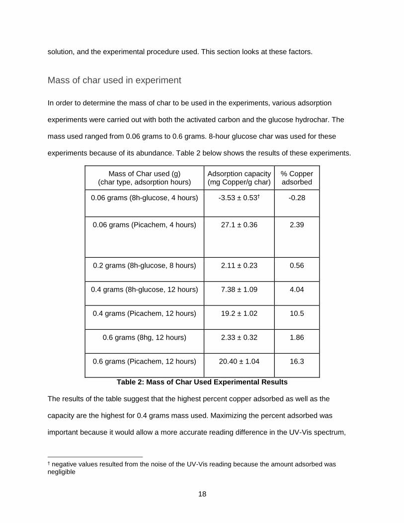
Mass of char used in experiment

In order to determine the mass of char to be used in the experiments, various adsorption

experiments were carried out with both the activated carbon and the glucose hydrochar. The

mass used ranged from 0.06 grams to 0.6 grams. 8-hour glucose char was used for these

experiments because of its abundance. Table 2 below shows the results of these experiments.

Mass of Char used (g) (char type, adsorption hours)

Adsorption capacity (mg Copper/g char)

% Copper adsorbed

0.06 grams (8h-glucose, 4 hours) -3.53 ± 0.53†

-0.28

0.06 grams (Picachem, 4 hours) 27.1 ± 0.36 2.39

0.2 grams (8h-glucose, 8 hours) 2.11 ± 0.23 0.56

0.4 grams (8h-glucose, 12 hours) 7.38 ± 1.09 4.04

0.4 grams (Picachem, 12 hours) 19.2 ± 1.02 10.5

0.6 grams (8hg, 12 hours) 2.33 ± 0.32 1.86

0.6 grams (Picachem, 12 hours) 20.40 ± 1.04 16.3

Table 2: Mass of Char Used Experimental Results

The results of the table suggest that the highest percent copper adsorbed as well as the

capacity are the highest for 0.4 grams mass used. Maximizing the percent adsorbed was

important because it would allow a more accurate reading difference in the UV-Vis spectrum,

† negative values resulted from the noise of the UV-Vis reading because the amount adsorbed was negligible

19

therefore maximizing accuracy. Because this MQP compared the capacities of the glucose

chars, the results of the glucose chars in the above table, rather than that of Picachem, were

used in determining the mass used.

Determining the Concentration of the Copper Nitrate Solution

Another parameter to determine was the concentration of copper nitrate solution to be used. It

was important that, in order to reduce errors in the calibration curve use, the concentration

range to be investigated be in the mid-range of the curve. Two concentrations were tested:

0.06M and 0.04M. Using a 0.4 g mass of 12-hour glucose, the adsorption capacity was

determined for these two concentrations. The raw data and sample calculations can be found in

Appendix III. The results are summarized in the Table 3 below.

Concentration used (char type, adsorption hours)

Adsorption capacity (mg Copper/g char)

0.04M (12h-glucose, 24 hours) 1.71 ± 0.14

0.06M (12h-glucose, 24 hours) 2.87 ± 0.46

Table 3: Concentration of Copper Nitrate Experimental Results

The table shows that 0.06M solution gives a better adsorption capacity. A higher value of the

capacity would also enable a better resolution, therefore more accurate results, while comparing

the capacities of different chars. As a result, 0.06M was chosen as the standard concentration

to be used.

Plastic vs. glass vials

There were two choices for the vials to be used in the wrist-action shaker: glass or plastic. An

experiment was run to determine if the capacity and/or error bars differed due to the type of vial.

0.4 grams of Picachem was used in a 0.06M solution of copper nitrate in both vials and shaken

20

for 19 hours. The difference in adsorption capacity between the two types of vials was just

1.84%, and showed that either option could be used. The glass vials were chosen because they

were easier to use and had higher availability in the lab. The raw data and sample calculations

can be found in Appendix IV.

Centrifuge vs. Vacuum Filtration

After the solution of copper nitrate was shaken with the chars, it had to be separated from the

chars in order to be used in the UV-Vis spectrophotometer. There were two different methods to

be used for the process: vacuum filtration or centrifugation.

In order to determine which method was better, 0.06M copper nitrate solution was shaken with

0.4 grams of Picachem for an arbitrary time of 20 hours. Then the solution was either vacuum

filtered or centrifuged at 4000 RPM for 5 minutes and then analyzed in the UV-Vis

spectrophotometer. The raw data and sample calculations can be found in Appendix V. The

results are summarized in the Table 4 below.

Procedure Used Adsorption capacity (mg Copper/g char)

Vacuum Filtration 23.6 ± 0.55

Centrifugation at 4000 RPM for 5 minutes 23.6 ± 0.11

Table 4: Filtration Method Experimental Results

The results show that the adsorption capacity were very similar. However, the major difference

was the presence of a larger error for the vacuum filtration method, which was probably due to

the increased chances of experimental errors while performing the filtration, or the interaction of

the solution with the filter paper. On the other hand, the centrifugation process was a quicker

process to separate the solution from the char, and many vials could be run in the centrifuge at

21

once. Because centrifugation saved time and gave better error bars, it was chosen as the

preferred method.

Equilibrium Curves

In order to compare the performance of different glucose hydrochars, a common adsorption

time was used to ensure consistency. The first step in determining this time was to plot the

adsorption capacity as a function of adsorption time for each char and the activated carbon,

Picachem HP-120. Because of time and material constraints, these plots, also known as

Equilibrium Curves, were made for the 8-, 16- and 24-hour glucose chars, and for Picachem.

The raw data can be found in Appendix VI. As seen in Figure 2, the adsorption capacity for the

8- and 16-hour glucose chars both peaked at 8 hours, while the 24-hour glucose peaked at 12

hours. After each curve peaks, the lines slowly decline until they reach a constant value referred

to as the equilibrium value. This behavior, however, was not observed for Picachem. Although

the true equilibration time for the hydrochars was much longer, we chose 24 hours as the

pseudo-equilibration time because the capacities at this time were close to the equilibrium

values, allowing us to carry out the experiments much quicker. All the experiments comparing

the performance of different chars were thus carried out at 24 hours. The raw data for the 24

hour experiments can be found in Appendix VII.

A closer look at the equilibrium curve for the glucose chars shows that the peak capacity falls by

ca. 30% before it reaches equilibrium. A plausible explanation to this large change is that its

structure breaks down in water during the course of the experiment, specifically after 8 hours. In

order to test this hypothesis, the pH of the copper nitrate solution containing the 8-hour glucose

char was measured at regular intervals to probe into the changing chemistry. The table below

includes the results of the pH test. The highest change in pH value was within the first 4 hours

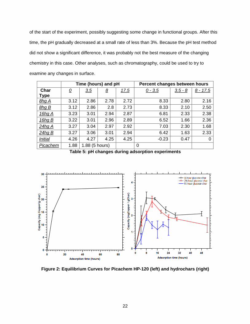
22

of the start of the experiment, possibly suggesting some change in functional groups. After this

time, the pH gradually decreased at a small rate of less than 3%. Because the pH test method

did not show a significant difference, it was probably not the best measure of the changing

chemistry in this case. Other analyses, such as chromatography, could be used to try to

examine any changes in surface.

Time (hours) and pH Percent changes between hours

Char Type

0 3.5 8 17.5 0 - 3.5 3.5 - 8 8 - 17.5

8hg A 3.12 2.86 2.78 2.72 8.33 2.80 2.16

8hg B 3.12 2.86 2.8 2.73 8.33 2.10 2.50

16hg A 3.23 3.01 2.94 2.87 6.81 2.33 2.38

16hg B 3.22 3.01 2.96 2.89 6.52 1.66 2.36

24hg A 3.27 3.04 2.97 2.92 7.03 2.30 1.68

24hg B 3.27 3.06 3.01 2.94 6.42 1.63 2.33

Initial 4.26 4.27 4.25 4.25 -0.23 0.47 0

Picachem 1.88 1.88 (5 hours)

0

Table 5: pH changes during adsorption experiments

Figure 2: Equilibrium Curves for Picachem HP-120 (left) and hydrochars (right)

23

Adsorption Capacity by Mass

The chars studied in this experiment were 4-, 8-, 12-, 16-, and 24- hour glucose chars, as well

as the activated carbon Picachem HP-120. Each char and activated carbon was shaken for 24

hours in 20 mL of 0.06M copper nitrate solution. Figure 3 shows the adsorption capacity for

each char and the activated carbon.

Figure 3: Adsorption Capacity by Mass

Figure 3 shows that Picachem HP-120 has a much higher the capacity compared to the chars,

and 4-hour glucose char has the highest capacity among the chars. We furthered this analysis

by comparing the surface area of each char with its adsorption capacity to see how much of an

influence the surface area had on the adsorption capacity. The surface areas were calculated

by DFT fit of nitrogen adsorption isotherm. Figure 4 below displays our findings.

24

Figure 4: Relationship between the adsorption capacity and surface area of hydrochars.

Char

type

DFT Surface Area

(m2/g)

4-hour glucose 11.531

8-hour glucose 3.445

12-hour glucose 2.801

16-hour glucose 2.826

24-hour glucose 2.732

Picachem HP-120 1454

Table 5: Surface Area of Chars

A first glance at figure 4 suggests that the surface area and adsorption capacity are positively

correlated. Since 4-hour char has the highest surface area, it would make sense that it would

also have the highest adsorption capacity per mass. A similar argument would stand for the

capacity difference between the activated carbon and the chars. The surface area of the

Picachem HP-120 is 1454 m 2/g compared to 11.5 m 2/g of the 4-hour glucose char (the char

with the largest surface area). However, it should be noted although the surface area of the

25

activated carbon is ca. 100 times larger than that of the char, its adsorption capacity is only 5

times larger. This means that the surface of the char is able to interact much more with the

heavy metals.

Adsorption Capacity by Surface Area

The data from our experiments was analyzed to determine which char had the best adsorption

capacity per surface area. Figure 5 below displays our results.

Figure 5: Adsorption Capacity by Surface Area

As expected, the activated carbon was outperformed by the chars on a surface area basis. In

fact, the chars were better by a factor of 50. However, it was not expected that the 12-hour

glucose char would perform better than the 4-hour glucose char, especially after looking at the

trend in Figure 4. This confirms that available surface area alone is not responsible for the

adsorption of copper ions. Rather, surface chemistry plays an important role in adsorption.

To get a better idea of why the adsorption capacity per surface area is so much greater for the

26

chars, infrared (IR) spectroscopy was used to look at the surface functional groups present.

Figure 6: IR Spectrum of different hydrochars compared with Picachem HP-120.

It can be seen that the hydrochars have significantly more oxygen-containing functional groups.

Figure 6 above shows the IR spectrum of three glucose chars and Picachem HP-120. The

activated carbon seems to have significantly less functional groups compared to the glucose

char. In particular, the glucose chars have strong carbonyl (C=O) and hydroxyl (-OH) signals.

These negatively (or partial negatively) charged oxygen groups in the carbonyl/hydroxyl groups

engage in ionic interactions with the copper (II) ions in solution, and account for the increased

adsorption. The lack of these functional groups in particular in the activated carbon explains why

the adsorption capacity per surface area is so low. These results are significant because it

confirms the possibility that glucose char could be used as an alternative for activated carbon.

The IR spectrum does a good job in explaining the difference in surface chemistry between the

glucose chars and Picachem HP-120. However, it cannot be used to compare the surface

chemistry between the different glucose chars because the IR spectra of each of these are

essentially identical.

27

In order to look at the differences between the surface chemistry of these chars, various

characterization techniques involving Raman Spectroscopy, X-ray photoelectron spectroscopy

(XPS) and Nuclear Magnetic Resonance (NMR) spectroscopy could be utilized. An example of

a Raman spectrum for an 8-hour glucose char is shown below. The two major peaks shown in

figure 7 are the defect peak (D-peak) around 1350 cm-1 and the Graphite peak (G-peak) around

1550 cm-1.

Figure 7: Raman Spectrum of 8-hour glucose hydrochar showing the D and G peaks.

Proper analysis of a Raman spectrum is important to determine the functional groups present.

The spectra has to be fitted with different peaks corresponding to the different functional groups,

such that sum of the area of the fitted individual peaks equal the area of the overall Raman

spectrum. There are several peak assignment techniques, some of which are described by Li et

al.‡ and Sadezky et al.§ This was, however, beyond the scope of this MQP.

‡ X. Li, J.-I. Hayashi and C.-Z. Li, Fuel, 2006, 85, 1700-1707. § A. Sadezky, H. Muckenhuber, H. Grothe, R. Niessner and U. Pöschl, Carbon, 2005, 43, 1731-1742.

28

Conclusion and Recommendations

Although internal surface area is considered to be the major surface property that

determines adsorption capacity, the results presented in this report show that there are more

factors to consider. Surface chemistry, for example, plays an equal, if not more important, role in

determining the amount of copper ions adsorbed onto the surface of the hydrochar. This

argument was supported by the observation that the 4-hour glucose char, despite having the

largest surface area of 11.5 m 2/g among the chars, performed poorly on a per surface area

basis against all the other glucose hydrochars. However, despite having 100 times the surface

area, Picachem only had 5 times the adsorption capacity per unit mass. In other words, the 12-

hour glucose char performed more than 50 times better on a per surface area basis. This result

was attributed to the electrostatic attraction between the Cu2+ ions in solution and the

electronegative oxygen atoms present on the char surface relating to the aldehyde, hydroxyl,

ketone, ester, phenolic and carboxyl functional groups. The specific role of each of these groups

on the adsorption capacity, however, could not be determined because it required spectroscopic

analysis outside the scope of this MQP.

An interesting behavior was also observed while determining the equilibrium time for the

hydrochars. The adsorption capacity seemed to peak around the 8-hour adsorption time, and

fell gradually until it reached a constant value after around 30 hours. This behavior was not

observed for Picachem HP-120, suggesting that the char was interacting with water during the

course of the experiment. The pH tests weakly proved this hypothesis as its value steadily

decreased with adsorption time. However, because the difference in pH readings was low,

another form of analysis, eg. Chromatography, could be employed to test this hypothesis.

There are many places to start if one wants to build on this work in the future. First of all,

the functional group evolution on the char surface with reaction time can be studied to help

explain the relationship with the adsorption capacities. Proper characterization of the chars is

29

therefore important in this regard. The second area that can be studied is the reaction of the

chars with water during the adsorption experiments, especially in the time range of 8-16 hours

and around the peak. The knowledge of the changing chemistry will prove to be vital because of

the insights it can provide on the char structure. The third area to build on could be chemical

treatment of the chars. Because of the presence of numerous oxygen groups on the char, it can

be treated with acids or other chemicals to add more functionality to the surface. This added

functionality could be used, in addition to adsorption site for heavy metals, as a heterogeneous

catalyst. Another area to build on is changing the reaction parameters like temperature,

concentration, reaction pressure, etc. and observe changes in the surface functionality, with an

ultimate goal of maximizing the usefulness of the char.

30

Works Cited

1 "Toxic Substances Portal - Copper." Centers for Disease Control and Prevention. Centers for Disease Control and Prevention, 30 Nov. 2016. Web. 2 "Impacts From Lead and Copper Corossion." Water Research Foundation, n.d. Web. 30 Nov. 2016. <http://www.waterrf.org/knowledge/distribution-system-management/FactSheets/DistributionSystemMgmt_LeadCopper_FactSheet.pdf> 3 Ibid. 4 "Drinking Water." Centers for Disease Control and Prevention. Centers for Disease Control and Prevention, 01 July 2015. Web. 30 Nov. 2016. <https://www.cdc.gov/healthywater/drinking/private/wells/disease/copper.html>. 5 "Impacts From Lead and Copper Corossion." Water Research Foundation, n.d. Web. 30 Nov. 2016. <http://www.waterrf.org/knowledge/distribution-system-management/FactSheets/DistributionSystemMgmt_LeadCopper_FactSheet.pdf> 6 "Drinking Water." Centers for Disease Control and Prevention. Centers for Disease Control and Prevention, 01 July 2015. Web. 30 Nov. 2016. <https://www.cdc.gov/healthywater/drinking/private/wells/disease/copper.html>. 7 Worch, Eckhard. Adsorption Technology in Water Treatment: Fundamentals, Processes, and Modeling. Berlin ; Boston: De Gruyter, 2012. Print. 8 Mohan, Dinesh et al. “Organic and Inorganic Contaminants Removal from Water with Biochar, a Renewable, Low Cost and Sustainable Adsorbent – A Critical Review.” Bioresource Technology 160 (2014): 191–202. CrossRef. Web. 9 Thompson, Kyle A. et al. “Environmental Comparison of Biochar and Activated Carbon for Tertiary Wastewater Treatment.” Environmental Science & Technology 50.20 (2016): 11253–11262. CrossRef. Web. 10 Shackley, S.; Clare, A.; Joseph, S.; McCarl, B. A.; Schmidt, H.-P. “Economic evaluation of biochar systems: current evidence and challenges.” Biochar for Environmental Management (2015): 812−851. CrossRef. Web. 11 Alibaba.com. 325 Mesh Powdered Activated Carbon Factory Price. Shanghai Feb. 12, 2016 12 Wikberg, Hanne et al. “Structural and Morphological Changes in Kraft Lignin during Hydrothermal Carbonization.” ACS Sustainable Chemistry & Engineering 3.11 (2015): 2737–2745. CrossRef. Web. 13 Román, S. et al. “Hydrothermal Carbonization as an Effective Way of Densifying the Energy Content of Biomass.” Fuel Processing Technology 103 (2012): 78–83. CrossRef. Web. 14 "Renewables." Bioenergy. International Energy Agency, n.d. Web. 22 Apr. 2017. https://www.iea.org/topics/renewables/subtopics/bioenergy 15 Kang, Shimin et al. “Characterization of Hydrochars Produced by Hydrothermal Carbonization of Lignin, Cellulose, d-Xylose, and Wood Meal.” Industrial & Engineering Chemistry Research 51.26 (2012): 9023–9031. CrossRef. Web. 16 Ibid. 17 Meyer, Sebastian, Bruno Glaser, and Peter Quicker. “Technical, Economical, and Climate-Related Aspects of Biochar Production Technologies: A Literature Review.” Environmental Science & Technology 45.22 (2011): 9473–9483. CrossRef. Web. 18 Funke, Axel, and Felix Ziegler. "Hydrothermal Carbonization of Biomass: A Summary and Discussion of Chemical Mechanisms for Process Engineering." Biofuels, Bioproducts and Biorefining, vol. 4, no. 2, 2010, pp. 160-177 19 Meyer, Sebastian, Bruno Glaser, and Peter Quicker. “Technical, Economical, and Climate-Related Aspects of Biochar Production Technologies: A Literature Review.” Environmental Science & Technology 45.22 (2011): 9473–9483. CrossRef. Web.

31

20 Ibid. 21 Aydıncak, Kıvanç et al. “Synthesis and Characterization of Carbonaceous Materials from Saccharides (Glucose and Lactose) and Two Waste Biomasses by Hydrothermal Carbonization.” Industrial & Engineering Chemistry Research 51.26 (2012): 9145–9152. CrossRef. Web. 22 Kambo, Harpreet Singh, and Animesh Dutta. “A Comparative Review of Biochar and Hydrochar in Terms of Production, Physico-Chemical Properties and Applications.” Renewable and Sustainable Energy Reviews 45 (2015): 359–378. CrossRef. Web. 23 Funke, Axel, and Felix Ziegler. "Hydrothermal Carbonization of Biomass: A Summary and Discussion of Chemical Mechanisms for Process Engineering." Biofuels, Bioproducts and Biorefining, vol. 4, no. 2, 2010, pp. 160-177 24 Ibid. 25 Sevilla, M. and Fuertes, Antonio B. (2009), Chemical and Structural Properties of Carbonaceous Products Obtained by Hydrothermal Carbonization of Saccharides. Chem. Eur. J., 15: 4195–4203. 26 Meyer, Sebastian, Bruno Glaser, and Peter Quicker. “Technical, Economical, and Climate-

Related Aspects of Biochar Production Technologies: A Literature Review.” Environmental

Science & Technology 45.22 (2011): 9473–9483. CrossRef. Web. 27 Kang, Shimin et al. “Characterization of Hydrochars Produced by Hydrothermal Carbonization of Lignin, Cellulose, d-Xylose, and Wood Meal.” Industrial & Engineering Chemistry Research 51.26 (2012): 9023–9031. CrossRef. Web. 28 Titirici, Maria-Magdalena et al. “Black Perspectives for a Green Future: Hydrothermal Carbons for Environment Protection and Energy Storage.” Energy & Environmental Science 5.5 (2012): 6796. CrossRef. Web. 29 Ibid. 30 Aydıncak, Kıvanç et al. “Synthesis and Characterization of Carbonaceous Materials from Saccharides (Glucose and Lactose) and Two Waste Biomasses by Hydrothermal Carbonization.” Industrial & Engineering Chemistry Research 51.26 (2012): 9145–9152. CrossRef. Web. 31 Falco, Camillo et al. “Hydrothermal Carbon from Biomass: Structural Differences between Hydrothermal and Pyrolyzed Carbons via 13C Solid State NMR.” Langmuir 27.23 (2011): 14460–14471. Print. 32 Lin, Yousheng et al. “A Mechanism Study on Hydrothermal Carbonization of Waste Textile.” Energy & Fuels 30.9 (2016): 7746–7754. CrossRef. Web. 33 Cai, Huaming et al. “One-Step Hydrothermal Synthesis of Carbonaceous Spheres from Glucose with an Aluminum Chloride Catalyst and Its Adsorption Characteristic for Uranium(VI).” Industrial & Engineering Chemistry Research 55.36 (2016): 9648–9656. CrossRef. Web. 34 Kang, Shimin et al. “Characterization of Hydrochars Produced by Hydrothermal Carbonization of Lignin, Cellulose, d-Xylose, and Wood Meal.” Industrial & Engineering Chemistry Research 51.26 (2012): 9023–9031. CrossRef. Web. 35 Baccile, Niki et al. “Structural Characterization of Hydrothermal Carbon Spheres by Advanced Solid-State MAS 13 C NMR Investigations.” The Journal of Physical Chemistry C 113.22 (2009): 9644–9654. CrossRef. Web. 36 Titirici, Maria-Magdalena et al. “Black Perspectives for a Green Future: Hydrothermal Carbons for Environment Protection and Energy Storage.” Energy & Environmental Science 5.5 (2012): 6796. CrossRef. Web. 37 Aydıncak, Kıvanç et al. “Synthesis and Characterization of Carbonaceous Materials from Saccharides (Glucose and Lactose) and Two Waste Biomasses by Hydrothermal Carbonization.” Industrial & Engineering Chemistry Research 51.26 (2012): 9145–9152. CrossRef. Web.

32

38 Kambo, Harpreet Singh, and Animesh Dutta. “A Comparative Review of Biochar and Hydrochar in Terms of Production, Physico-Chemical Properties and Applications.” Renewable and Sustainable Energy Reviews 45 (2015): 359–378. CrossRef. Web. 39 Ibid. 40 Ibid. 41 Ibid. 42 Mahtab Ahmad, Anushka Upamali Rajapaksha, Jung Eun Lim, Ming Zhang, Nanthi Bolan, Dinesh Mohan, Meththika Vithanage, Sang Soo Lee, Yong Sik Ok, Biochar as a sorbent for contaminant management in soil and water: A review, Chemosphere, Volume 99, March 2014, Pages 19-33, ISSN 0045-6535 43 Kambo, Harpreet Singh, and Animesh Dutta. “A Comparative Review of Biochar and Hydrochar in Terms of Production, Physico-Chemical Properties and Applications.” Renewable and Sustainable Energy Reviews 45 (2015): 359–378. CrossRef. Web. 44 Barakat, M.A. “New Trends in Removing Heavy Metals from Industrial Wastewater.” Arabian Journal of Chemistry 4.4 (2011): 361–377. CrossRef. Web. 45 Ibid. 46 Aziz, Hamidi A., Mohd. N. Adlan, and Kamar S. Ariffin. “Heavy Metals (Cd, Pb, Zn, Ni, Cu and Cr(III)) Removal from Water in Malaysia: Post Treatment by High Quality Limestone.” Bioresource Technology 99.6 (2008): 1578–1583. CrossRef. Web. 47 Kurniawan, Tonni Agustiono et al. “Physico–chemical Treatment Techniques for Wastewater Laden with Heavy Metals.” Chemical Engineering Journal 118.1–2 (2006): 83–98. CrossRef. Web. 48 Barakat, M.A. “New Trends in Removing Heavy Metals from Industrial Wastewater.” Arabian Journal of Chemistry 4.4 (2011): 361–377. CrossRef. Web. 49 Kurniawan, Tonni Agustiono et al. “Physico–chemical Treatment Techniques for Wastewater Laden with Heavy Metals.” Chemical Engineering Journal 118.1–2 (2006): 83–98. CrossRef. Web 50 Kambo, Harpreet Singh, and Animesh Dutta. “A Comparative Review of Biochar and Hydrochar in Terms of Production, Physico-Chemical Properties and Applications.” Renewable and Sustainable Energy Reviews 45 (2015): 359–378. CrossRef. Web. 51 Alibaba.com. 325 Mesh Powdered Activated Carbon Factory Price. Shanghai February 12, 2016

33

Appendices

Appendix I- Detailed Lab Procedure

Preparing the samples

1. The copper nitrate solution used is 0.06M. The amount of water and copper nitrate is

based on the number of samples being tested. For each experiment, there are two vials

containing char and copper nitrate solution, and one vial containing just the initial copper

nitrate solution.

a. The amount of copper nitrate used was 0.2791 g per sample. The copper nitrate

was measured in an Erlenmeyer flask using a balance*.

b. Once the appropriate mass was in the beaker, 20 mL of DI water multiplied by

the number of samples was measured out using a graduated cylinder*. The

water was then added to the flask and stirred with a magnetic stirrer for 20

minutes. The flask was covered with parafilm to ensure no vapor escaped.

2. While the solution is being stirred, measure out 0.4000 ±0.008g of char in each vial*.

3. Using a pipette, transfer 20 mL of copper nitrate solution into each vial.

4. Place the vials into the shaker and turn the wrist-action shaker on.

Analyzing the Samples

1. After the samples have been shaken for the desired amount of time, take both samples

and the vial containing its initial solution out of the shaker.

2. Transfer the contents of the vials into their own plastic vial. The plastic vial is designed

for the centrifuge which will be used for filtration.

3. The vials are then placed in the centrifuge as described in the figure below. It is

important to keep the centrifuge balanced. If only three samples are going into the

centrifuge, fill three plastic vials with about 20 mL of water each and place on the other

side.

4. Set the centrifuge to 4000 rpm and run for 5 minutes.

5. After the centrifuge has come to a complete stop, take out the plastic vials. The solid

char should be at the bottom and liquid copper nitrate solution at the top of the vial.

Using a syringe, suction out the copper nitrate solution and place it in a clean glass vial.

Do this for each vial.

6. Start the UV machine, and before opening up the Software, make a new folder with its

name as the date.

7. DI water is used as a blank before any samples can be tested.

8. Using a syringe, suction out some of the solution from the vial. Place the filter on the

syringe and then transfer the liquid into the cuvette. Place the cuvette with the logo

facing towards the machine, and use the software to run the machine. Find the peak of

the curve*.

34

a. Repeat this at least two more times for this sample** Shake the vial for about 5

seconds before doing another reading to ensure the copper is equally distributed

throughout the solution.

i. Example for saving the file: 8HG12HA (8-hour glucose 12 hour shake)

ii. Clear data on software before collecting data from other samples

b. Repeat step 8 for sample b and the initial solution.

*Record in notebook

**Do more readings if a lot of variation

Appendix II- Calibration Curve Raw Data

Concentration AU 1 AU 2 St dev Error

0.08 0.915881 0.916729 0.000424 0.000299813

0.07 0.80658 0.804975 0.0008025 0.000567453

0.06 0.691442 0.694518 0.001538 0.00108753

0.05 0.577569 0.573232 0.0021685 0.001533361

0.04 0.468702 0.46699 0.000856 0.000605283

0.03 0.36121 0.356354 0.002428 0.001716855

0.02 0.23962 0.238038 0.000791 0.000559321

0.01 0.11933 0.120246 0.000458 0.000323855

Appendix III- Amount of Char Used Raw Data

35

Appendix IV- Centrifuge vs. Vacuum Filtration Raw Data

Vial# Hours AU 1 AU 2 AU 3 Average Capacity

Final Capacity

Error

19A cent 19 0.606206 0.605648 0.605776 23.79455

19B cent 19 0.607662 0.606864 0.607821 23.30655 23.55055 0.106973

19C (filt) 19 0.612567 0.612038 0.61118 24.11676

19D (filt) 19 0.622119 0.618215 0.607034 23.01221 23.56448 0.565401

Appendix V- Equilibrium Curve Raw Data

8-hour glucose hydrochar

Vial# Hours AU 1 AU 2 AU 3 Average Capacity

Final Capacity

Error

4A 4 0.68996 0.689356 0.691997 3.797334

4B 4 0.704525 0.705103 0.705861 -0.3329 1.732216 0.849187

8A 8 0.687842 0.688097 0.687739 3.875468

8B 8 0.693451 0.695867 0.692032 2.244261 3.059864 0.357088

14A 14 0.677163 0.677215 0.678828 3.086873

14B 14 0.678313 0.678342 0.678016 2.946855 3.01686 0.069866

22A 22 0.694569 0.693853 0.696004 2.729896

22B 22 0.697221 0.696986 0.698666 1.940193 2.335044 0.186599

29A 29 0.681287 0.685472 0.684958 6.924086

29B 29 0.67344 0.675395 0.675292 9.491891 2.017993 0.131555

48A 48 0.699479 0.699298 0.7011 2.103738 2.103738 0.130933

Average Initial

Init 4 4 0.704909 0.703872 0.703149 0.703977

Init 8 8 0.700786 0.702425 0.702096 0.701769

Init 14 14 0.68811 0.688648 0.689441 0.688733

Init 22 22 0.704688 0.704531 0.704443 0.704554

Init 29 29 0.708596 0.707739 0.709573 0.708636

Init 48 48 0.706471 0.70738 0.708573 0.707475

16-hour glucose hydrochar

Vial# Hours AU 1 AU 2 AU 3 Average Capacity

Final Capacity

Error

4A 4 0.702638 0.709387 0.710889 0.891726

4B 4 0.708702 0.71007 0.710653 0.284191 0.587959 0.322431

8A 8 0.694995 0.710134 0.712787 2.12522

8B 8 0.712567 0.713604 0.71379 1.604909 1.865065 0.163635

12A 12 0.704705 0.709737 0.709677 1.633223

12B 12 0.709245 0.709898 0.709577 1.202383 1.417803 0.211222

36

Vial# Hours AU 1 AU 2 AU 3 Average Capacity

Final Capacity

Error

16A 16 0.702017 0.710752 0.712524 2.005421

16B 16 0.714259 0.714839 0.715469 0.289416 1.147419 0.524663

20A 20 0.69243 0.702971 0.702983 1.709339

20B 20 0.706034 0.704545 0.703491 1.229847 1.469593 0.507702

24A 24 0.692358 0.701871 0.711514 1.956775

24B 24 0.710792 0.71264 0.713315 0.399801 1.178288 0.870381

Average Initial

Init 4 4 0.711019 0.710485 0.71096 0.710821

Init 8 8 0.71732 0.71907 0.720746 0.719045

Init 12 12 0.713048 0.712899 0.71565 0.713866

Init 16 16 0.716253 0.715587 0.714898 0.715579

Init 20 20 0.70953 0.708645 0.709076 0.709084

Init 24 24 0.713433 0.713057 0.714528 0.713673

24-hour glucose hydrochar

Vial# Hours AU 1 AU 2 AU 3 Average Capacity

Final Capacity

Error

4A 4.5 0.70488 0.705272 0.706203 2.355614

4B 4.5 0.708666 0.711992 0.710993 1.002028 1.678821 0.305317

8A 8 0.690001 0.690175 0.691942 2.422055

8B 8 0.692338 0.692603 0.694218 1.770331 2.096193 0.164997

12A 12 0.698321 0.699246 0.701491 3.403007

12B 12 0.701762 0.702081 0.707379 2.265825 2.834416 0.330251

18A 18.5 0.703932 0.704678 0.706436 2.346998

18B 18.5 0.705998 0.705733 0.706003 2.096383 2.22169 0.099522

24A 24 0.675905 0.679855 0.676509 1.876001

24B 24 0.676503 0.677893 0.677496 1.905074 1.890537 0.148591

30A 30 0.712474 0.711176 0.713025 1.940709

30B 30 0.712324 0.713688 0.713875 1.63952 1.790115 0.104171

Average Initial

Init 4 4.5 0.713333 0.713333 0.714904 0.713857

Init 8 8 0.703036 0.698692 0.696381 0.699370

Init 12 12 0.711342 0.711292 0.712805 0.711813

Init 18 18.5 0.712718 0.712188 0.715313 0.713406

Init 24 24 0.684206 0.684142 0.683972 0.684107

Init 30 30 0.719884 0.717967 0.719577 0.719143

37

Appendix VI- Each char at 24 hour shake Raw Data

Vial# AU 1 AU 2 AU 3 Average Capacity Final Capacity

Error

4A 0.68509 0.69386 0.69521 7.090568908

4B 0.69921 0.7003 0.70119 4.735174305 5.912872 0.627907

8A 0.694569 0.693853 0.696004 2.729896075

8B 0.697221 0.696986 0.698666 1.940192538 2.335044 0.186599

12A 0.76018 0.761581 0 3.91291835

12B 0.767797 0.768504 0.768656 1.82302199 2.86797 0.462678

16A 0.675372 0.675696 0.675592 2.39838555

16B 0.675896 0.677992 0.67686 2.015784824 2.207085 0.104996

24A 0.675905 0.679855 0.676509 1.876000736

24B 0.676503 0.677893 0.677496 1.905074164 1.890537 0.148591

12A (0.04M) 0.459834 0.456036 0.457542 1.706064423

12B (0.04M) 0.456983 0.457597 0.45874 1.710393991 1.708229 0.139649

24A 0.639585 0.639209 0.639911 23.92889817

24B 0.638505 0.638215 0.639627 24.18564715 24.05727 0.075655 Average Initial

Init 4 0.71838 0.71499 0.71667 0.71668

Init 8 0.704688 0.704531 0.704443 0.704554

Init 12 0.774265 0.774914 0.775253 0.774811

Init 16 0.684206 0.684142 0.683972 0.684107

Init 24 0.684206 0.684142 0.683972 0.684107

Init 12 (0.04M) 0.467223 0.460811 0.463599 0.463878

Appendix VII- Sample Calculations

For the following calculations, the data for Vial# 4A and 4B listed in the table in Appendix VII are

used:

Vial# AU 1 AU 2 AU 3 Average Capacity

Final Capacity

Error

4A 0.68509 0.69386 0.69521 7.090568908

4B 0.69921 0.7003 0.70119 4.735174305 5.912872 0.627907

Average Initial

Init 4 0.71838 0.71499 0.71667 0.71668

In order to determine the final capacity of the hydrochar from the UV-Vis absorption data, each

of the three Absorption Units (AU 1, AU 2 and AU 3) were first converted, using the calibration

curve equation, to concentration:

38

0.68509 − 0.0119

11.334= 0.059395624 M

This value is then converted to grams of Copper by first determining the number of moles of

copper nitrate solution and then multiplying it by the molar mass of copper:

(0.059395624 𝑀 ∗ 0.02 𝐿) ∗ 63.546 𝑔/𝑚𝑜𝑙 = 0.075487086 𝑔

Similarly, for the initial value of 0.71838:

0.71838 − 0.0119

11.334= 0.062332804 M

Converting to grams of copper

(0.062332804 𝑀 ∗ 0.02 𝐿) ∗ 63.546 𝑔/𝑚𝑜𝑙 = 0.079220007 𝑔

Now, calculate the mass of copper adsorbed, divide by the mass of hydrochar used, and

multiply by 1000 to convert to milligrams:

0.079220007𝑔 − 0.075487086 𝑔

0.4 𝑔∗ 1000

𝑚𝑔

𝑔= 8.855735574

𝑚𝑔 𝐶𝑜𝑝𝑝𝑒𝑟

𝑔 𝑐ℎ𝑎𝑟

These steps were applied to all the 6 readings in vials 4A and 4B, and the average capacities

calculated. The errors were calculated using:

𝐸𝑟𝑟𝑜𝑟 =𝑆𝑡𝑎𝑛𝑑𝑎𝑟𝑑 𝑑𝑒𝑣𝑖𝑎𝑡𝑖𝑜𝑛 𝑜𝑓 𝑎𝑙𝑙 𝑡ℎ𝑒 𝑐𝑎𝑙𝑐𝑢𝑙𝑎𝑡𝑒𝑑 𝑐𝑎𝑝𝑎𝑐𝑖𝑡𝑖𝑒𝑠

√(𝑁𝑢𝑚𝑏𝑒𝑟 𝑜𝑓 𝑜𝑏𝑠𝑒𝑟𝑣𝑎𝑡𝑖𝑜𝑛𝑠)