analysis of horizontal reactive scaling on container
TRANSCRIPT
MASTER’S DEGREE IN PARALLEL AND DISTRIBUTED
COMPUTING
Academic Course 2015 / 2016
Master’s Degree Thesis
Analysis of Horizontal Reactive Scaling
on Container Management Systems
September, 2016
Student:
César González Segura
Supervisor:
Germán Moltó Martínez
Elasticidad Horizontal Reactiva Basada en Contenedores


Acknowledgements
I want to thank the members of the GRyCAP research group, Germán Moltó, Ignacio
Blanquer and Damián Segrelles for giving me the opportunity to work in this project and
for their support. The effort done by my supervisor, German, has greatly helped me finish
this project thanks to his advice and guidance.
I also want to thank all my colleagues at the master’s course for their support and
company through this very intense year. And finally, to my girlfriend and my family for
their unconditional support on all my projects.
César González Segura
iii.


Abstract
Container management systems have appeared recently as an alternative to virtual
machines, offering relative isolation without the overhead of running virtual machines (VMs).
Containers are attractive for its use in distributed systems thanks to its horizontal scaling
properties. In this project, the performance of virtual machines and the Kubernetes container
management system is evaluated, in order to compare the computing performance and
economic cost of both alternatives.
Resumen
Los sistemas de gestión de contenedores han surgido recientemente como una
alternativa a las máquinas virtuales, ofreciendo un aislamiento relativo sin el overhead de
las máquinas virtuales (VMs). Gracias a sus propiedades de escalabilidad horizontal, los
contenedores son una alternativa interesante para el uso en sistemas distribuidos. En este
proyecto se evalúa el rendimiento de las máquinas virtuales y del sistema de gestión de
contenedores Kubernetes, con el objetivo de establecer una comparativa de la capacidad de
cómputo y del coste económico de ambas alternativas.
Resum
Els sistemes de gestió de contenidors han sorgit recentment com una alternativa a
les màquines virtuals, oferint un aïllament relatiu sense el overhead de les màquines virtuals
(VMs). Gràcies a les seues propietats d’escalabilitat horitzontal, els contenidors són una
alternativa interesant per al seu us en sistemes distribuïts. En aquest projecte s’avalua el
rendiment de les màquines virtuals i del sistema de gestió de contenidors Kubernetes, amb
l’objectiu d’establir una comparativa de la capacitat de còmput i del cost econòmic
d’ambdues alternatives.
v.


Contents
1 Introduction
1.1 Motivation
1.2 Objectives
1.3 Structure
2 State of the art
2.1 Previous work
2.2 Technology review
2.3 Amazon Web Services
2.4 Kubernetes
3 Environment set-up
3.1 Toolchain
3.2 Test application
3.3 Client metrics measurement
3.4 Infrastructure metrics measurement
4 Tests
4.1 Test bench
4.2 Test results
4.2.1 Small profile test results
4.2.2 Medium profile test results
4.2.3 Large profile test results
4.3 Results discussion
4.4 Cost evaluation
5 Conclusions
5.1 Future work
vii.
10
11
12
12
16
16
17
19
20
23
23
23
25
27
30
30
31
31
33
35
37
38
40
40
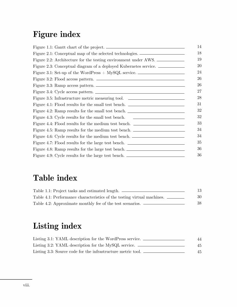
Figure index
Figure 1.1: Gantt chart of the project.
Figure 2.1: Conceptual map of the selected technologies.
Figure 2.2: Architecture for the testing environment under AWS.
Figure 2.3: Conceptual diagram of a deployed Kubernetes service.
Figure 3.1: Set-up of the WordPress + MySQL service.
Figure 3.2: Flood access pattern.
Figure 3.3: Ramp access pattern.
Figure 3.4: Cycle access pattern.
Figure 3.5: Infrastructure metric measuring tool.
Figure 4.1: Flood results for the small test bench.
Figure 4.2: Ramp results for the small test bench.
Figure 4.3: Cycle results for the small test bench.
Figure 4.4: Flood results for the medium test bench.
Figure 4.5: Ramp results for the medium test bench.
Figure 4.6: Cycle results for the medium test bench.
Figure 4.7: Flood results for the large test bench.
Figure 4.8: Ramp results for the large test bench.
Figure 4.9: Cycle results for the large test bench.
Table index
Table 1.1: Project tasks and estimated length.
Table 4.1: Performance characteristics of the testing virtual machines.
Table 4.2: Approximate monthly fee of the test scenarios.
Listing index
Listing 3.1: YAML description for the WordPress service.
Listing 3.2: YAML description for the MySQL service.
Listing 3.3: Source code for the infrastructure metric tool.
viii.
14
18
19
20
24
26
26
27
28
31
32
32
33
34
34
35
36
36
13
30
38
44
45
45


Chapter 1
Introduction
Since the first network services started operating, there has been a great interest in delivering
the best performance to the users while minimizing the expenses needed to run the system.
However, said perceived performance can vary depending on the concurrent number of
clients connected to the system.
Ideally, all systems should be designed and deployed to concurrently handle as many
connections as requested by its clients. Failing to do so may frustrate many users, which
could stop using the platform altogether. Even though this issue is not new many modern
services suffer of the Slashdot effect [Adler99]
, failing to correctly estimate the number of users
the service will have on its launch and losing potential users and customers.
Designing and deploying networked and concurrent systems has always supposed a
challenge. The first systems relied on cluster systems based on fixed hardware, which had to
be purchased or rented by the service provider and operated manually.
If the provisioned hardware could not satisfy the demand, the service had to be shut
down in order to add additional nodes to the cluster, and started again, generating a
disruption in service. Moreover, services designed to accommodate the maximum peak of
clients at a given time would be greatly underutilized at all other times, generating
unnecessary expenses.
To put said underutilized resources to use, the grid initiative was born as a way to
connect computing clusters over the network and use the available resources on remote
machines [Berman03]. Further advances thanks to the experience with the grid initiative plus
advances on machine virtualization led to what is currently known as cloud computing, which
is the focus of this work.
10

1.1 Motivation
Cloud computing is defined by the USA’s NIST as “(···) a model for enabling (···) on-demand
network access to a shared pool of (···) computing resources that can be rapidly provisioned
(···) with minimal effort” [Mell11]
. From an infrastructure point of view, cloud systems are
usually composed of a collection of interconnected cluster systems, sharing computing and
storage resources over the network.
Virtualization is the key to manage all the aggregate resources that form cloud
networks. Over the bare metal hardware, instances of virtual machines and storage devices
can be created and destroyed, enabling developers to scale their services to the demand and
avoiding problems such as stated earlier.
The popularization of public cloud providers and virtualization has opened new
possibilities for adjusting the expenses to the minimum. When the user load is low, services
can scale to the minimum number of computing resources needed, if the load increases, the
service can instantiate new virtual machines, scaling the capacity of the service to
accommodate the increased number of clients.
Even though services backed by virtual machines do not take a lot of time to scale
(usually in several minutes), there are situations where the increase in load is fast enough to
not let the service process all the incoming requests before it scales to the new capacity.
One of the solutions to this problem that is recently gaining momentum recently is
deploying services on container based systems [Merkel14]
. Containers are a lightweight instance
of an operating environment, that can be run on physical and virtual machines and provide
good isolation in terms of performance but their isolation in terms of security is not as
complete as when using VM’s. One of its benefits over virtual machines is the capacity of
scaling in seconds instead of minutes, which should in theory let systems scale in time and
minimize the impact on the user level experience during a load increase.
The main motivation of this project is assessing if there is a real benefit on the use
of these container based solutions instead of traditional virtual machines, from a performance
and economic perspective. If this was the case, many more developers may be tempted to
port their services to a container based deployment.
11

1.2 Objectives
Given the motivations stated previously, the main objective of this project is creating an
environment to test the computing performance and horizontal scaling capabilities of systems
backed by traditional virtual machines and by container management systems, using defined
metrics to make a comparison. The complete list of objectives is:
Analyzing the available public and private cloud providers and container
management systems, to select the backend that suites best to conduct the tests.
Setting-up the test environment to ensure that the tests can be repeated and that
the results are reproducible.
Creating the declarative definitions to deploy the test application to the
infrastructure, for both virtual machine and container deployments.
Set-up the necessary tooling to obtain the comparison metrics, and develop any
additional tooling that might be necessary.
Obtain the computational and economic performance of the test scenario.
1.3 Structure
The project is divided in the following chapters. Chapter 2 consists of a small review of the
state of the art of research on service scaling under container based architectures. Chapter
3 does a review of some of the most common public and private cloud providers and container
management systems, and introduces the selected providers, Amazon Web Services and
Kubernetes. Chapter 4 explains the environment used to conduct the tests, and in chapter
5 the test bench and results are commented. Finally, chapter 6 is dedicated to the future
work.
12
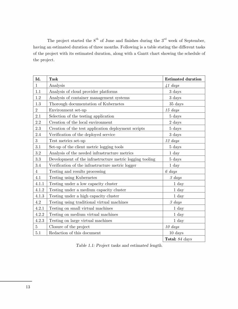
The project started the 8th of June and finishes during the 3
rd week of September,
having an estimated duration of three months. Following is a table stating the different tasks
of the project with its estimated duration, along with a Gantt chart showing the schedule of
the project.
Id. Task Estimated duration
1 Analysis 41 days
1.1 Analysis of cloud provider platforms 3 days
1.2 Analysis of container management systems 3 days
1.3 Thorough documentation of Kubernetes 35 days
2 Environment set-up 15 days
2.1 Selection of the testing application 5 days
2.2 Creation of the local environment 2 days
2.3 Creation of the test application deployment scripts 5 days
2.4 Verification of the deployed service 3 days
3 Test metrics set-up 12 days
3.1 Set-up of the client metric logging tools 5 days
3.2 Analysis of the needed infrastructure metrics 1 day
3.3 Development of the infrastructure metric logging tooling 5 days
3.4 Verification of the infrastructure metric logger 1 day
4 Testing and results processing 6 days
4.1 Testing using Kubernetes 3 days
4.1.1 Testing under a low capacity cluster 1 day
4.1.2 Testing under a medium capacity cluster 1 day
4.1.3 Testing under a high capacity cluster 1 day
4.2 Testing using traditional virtual machines 3 days
4.2.1 Testing on small virtual machines 1 day
4.2.2 Testing on medium virtual machines 1 day
4.2.3 Testing on large virtual machines 1 day
5 Closure of the project 10 days
5.1 Redaction of this document 10 days
Total: 84 days
Table 1.1: Project tasks and estimated length.
13

Figure 1.1: Gantt chart of the project
14


Chapter 2
State of the Art
This chapter is divided in two sections. The first is a brief introduction to the previous
research efforts in work related to this project. The second part is dedicated to analyzing
the available virtual machine and container management system technologies, in order to
choose the technologies that suit better this project.
Even though in the existing literature there are numerous articles dedicated to
distributed systems, container based systems are relatively recent and research material on
the subject is relatively scarce. From the available literature, two articles have been chosen
to serve as a basis for this project. Both articles stablish a comparison between container
based services and traditional virtual machines, but taking different approaches.
2.1 Previous Work
The first article is “Performance Comparison Between Linux Containers and Virtual
Machines”, by Ann Mary Joy [Joy15]. Taking the results of previous work related to
performance of traditional virtual machines, in this article the author creates a test bench
on Amazon EC2 and Kubernetes, using Joomla and WordPress as the test applications.
The application was flooded with requests on 10 minute intervals, and from the
obtained results the author concluded that Kubernetes (and container management systems
in general) yield better response times and scaling properties when compared to virtual
machines, having a speed-up of 22x on scaling reaction times.
The second article is “An Updated Performance Comparison of Virtual Machines and
Linux Containers”, by Wes Felter and others. In this article, the authors create a test bench
using MySQL as the test application, KVM as the virtual machine hypervisor and Docker
as the container manager. Given their results, the authors conclude that containers yields
better scaling properties due to the minimum CPU overhead, while the IO throughput is
worse than on traditional virtual machines.
16

However, the authors explain that to obtain good performance on both virtual
machines and containers, the underlying management systems must be correctly configured,
which requires having a deep understanding of the platform. Results obtained by similar
tests could not be representative of the general behavior of virtual machines or containers
due to misconfigured managers.
Taking these two publications as a foundation, the next step involves evaluating the
existing technologies to create the performance tests for this project.
2.2 Technology Review
The technology review for this project involves analyzing existing technologies and services
for deploying virtual machines and containers. Evaluating the pros and cons of each, the
technologies that are most fit for the project will be used. Then, the selected technologies
will be explained with more detail to have a better understanding of how the tests will be
conducted.
Since the test application has to be executed on virtual machines, a suitable
hypervisor or management system is needed. To simplify the deployment process and make
testing easier, instead of focusing on using a hypervisor and creating the virtual machines
over it (such as VMware ESX), the study will focus on the available public and private
cloud providers.
Cloud providers let users instantiate and destroy virtual machines (along with
storage devices, network devices and more) in a simple and fast way. Depending on how
access is granted to these cloud environments, these could be further divided into public and
private cloud providers.
Private providers offer enterprises and institutions solutions to create a cloud
environment on their own premises, in order to make a better use of their available
computing resources. Two of the most used private cloud providers are OpenStack and
OpenNebula. Even though it would have been possible to conduct the tests in the GRyCAP’s
private cloud environment, using a public cloud provider was decided to facilitate
reproducibility of the experiments conducted on this work by other researchers.
Public cloud providers rent their computing resources, where users can instantiate
virtual machines, storage elements, network devices and others for a fee. Following the NIST
definition of cloud computing [Mell11], this would be the case of a service following the IaaS
model (infrastructure as a service). This enables developers to create their services in a pay-
per-use fashion, only spending money for the needed computing power at any given time.
17

Two of the most popular public cloud providers are Amazon Web Services and
Microsoft Azure. AWS offers a very extensive catalog of virtual machine images, has a great
number of support resources and is very well integrated in the Linux ecosystem, which will
be a plus to easily conduct the tests. Microsoft Azure offers a very similar service; however,
it is more centered towards their own ecosystem. For these reasons the selected public cloud
provider is Amazon Web Services.
On the other hand, the choice for container management systems is not as wide as
with hypervisors or cloud providers. Cloud providers offer container management solutions,
such as Amazon ECS, OpenStack’s Nova-Docker[Nova]
or the OneDock development to
introduce Docker support in OpenNebula [Dock]
.
One of the most used container management systems, which is considered by many
as an industry standard, is Kubernetes, developed internally by Google to be used for their
internal workloads and now powering their public cloud container service, Google Compute
Engine. Since this container management system is one of the best maintained solutions and
it is considered an industry standard by many, it has been considered the best choice for the
project.
In conclusion, the technologies that will be used to conduct the tests needed for this
project are Amazon Web Services for the virtual machine tests and Kubernetes for the
container based tests. In the next section, both technologies are explained with greater detail
to understand how are the tests going to be conducted.
Figure 2.1: Conceptual map of the selected technologies.
18

2.3 Amazon Web Services
As stated in the previous section, Amazon Web Service (AWS for short) offers different
kinds of computing resources for a fee. In this project, AWS will be used to create the virtual
machines for the testing and to support Kubernetes. To achieve this, the following AWS
services will be used:
EC2 (Elastic compute cloud): Offers the creation of virtual machines with different
performance ranges, from small machines featuring a single core and less than a
gigabyte of memory to machines with dozens of cores and tens of gigabytes of memory.
Amazon offers a virtual machine image repository with thousands of preconfigured
operating systems to be used on the EC2 instances.
ELB (Elastic Load Balancers): A service inside EC2 which creates a networking
element able to balance the load coming from the outside to a distributed system
between its different instances.
Auto Scaling Groups: Instead of launching individual EC2 instances, a group can be
created where the service scales the number of instances automatically depending on
a set of predefined metrics (CPU usage, memory usage, among others).
Using said services as the foundations, the Kubernetes cluster and the virtual
machines for testing the application will be deployed. To control the service and the created
instances, AWS offers both a web GUI interface and a console command line tool called
awscli. While the GUI interface is useful for creating instances easily, the command line
tool will be useful to act as a bridge with the AWS API to obtain testing metrics.
The following figure represents the testing environment using AWS. The different
elements of Kubernetes and the testing environment will be detailed subsequently.
Figure 2.2: Architecture for the testing environment under AWS.
19

2.4 Kubernetes
Kubernetes has to be deployed on a machine cluster, where the containers will be evenly
distributed to balance the workload between the available nodes. These nodes follow a
master-slave relationship, where the master acts as the controller for all the slave nodes and
routes the traffic in and out of the cluster. In the bibliography, slave nodes are known as
minions.
Even though Kubernetes uses containers, the smallest computing resource available
to the user is the pod. A pod is a computing element that can contain one or more containers
along with its storage resources, enabling services to be tightly coupled together.
Launching individual pods with a single container is considered a bad practice, since
one of the main advantages of using containers is being able to recover fast from a failure,
and pods are not fail tolerant by themselves.
To solve this, services enable users to create a group of pods which share the same
image, are failure-tolerant and can be scaled up to a set number of instances. A service can
have an external entry point assigned to a single port, or as a load balancer to distribute the
load through all the instanced pod replicas.
The third important feature of Kubernetes are horizontal pod autoscalers
(HPA). HPA’s monitor a set of defined metrics on the pods inside a service, and change
the number of instances accordingly (for example, depending on the CPU load or memory
consumption). With all this three features, the behavior of Amazon EC2, ELB and ASG can
be replicated using containers.
Figure 2.3: Conceptual diagram of a deployed Kubernetes service.
20
The Kubernetes cluster can be configured from both a web based GUI interface and
from a command line interface called kubectl, as with AWS. Since the GUI interface does
not have the full feature set of the command line interfaced, it will not be used.
A very powerful feature of Kubernetes is the ability to deploy complete services using
declarative descriptions, defined through JSON or YAML recipes. These recipes have all the
definitions for the pods, services and horizontal scalers that the service must use to work.
With this feature, tests are guaranteed to be reproducible on different scenarios, and easily
replicable.
Along with the bare Kubernetes software, the default Kubernetes distribution comes
with other useful plugins such as Grafana [Graf]
, a web tool to visualize performance metrics
and debug services, and Heapster [Heap]
, a service that collects different metrics from the
services and exposes them with a simple REST API. Both services will be useful to build
the tests and the metric measurement tools.
In order to deploy the cluster into AWS, Kubernetes distribution comes with tools
to automatically create and destroy the required EC2 instances and other computing
resources on the cloud. Thanks to this, launching a new cluster becomes a simple and fast
task, taking mere minutes.
Now that the main technologies that are going to be used to conduct the tests have
been introduced, the next chapter will deal with the design and implementation of the
environment used to conduct the tests.
20


Chapter 3
Environment Set-up
This chapter is dedicated to describing how the environment for conducting the tests is
created. In order to do the performance analysis, a service is used under both virtual
machines and containers. Then, taking into account the relevant metrics for the test, a
framework to test the client perceived performance and the infrastructure performance is
designed and implemented.
3.1 Toolchain
To be able to obtain reliable and reproducible results, creating a good testing toolchain is a
necessity. This toolchain is the collection of tools to deal with the creation and destruction
of the Kubernetes cluster, creating the test application, obtaining metrics and processing
them.
This toolchain will run on a Linux virtual machine, to ease working from different
environments. The selected Linux distribution is Debian Linux, using VirtualBox as its
hypervisor. This machine is then configured with an installation of the Kubernetes
distribution, of the AWS command line interface and with the required credentials to access
AWS from the console. Having a local installation of Kubernetes is necessary to use its
command line interface.
The next step is selecting a test application, and designing the recipes required to
instantiate the service in both virtual machines and Kubernetes.
3.2 Test Application
A suitable test application should be one that can show the differences between working on
virtual machines and working on a container management system. It should require some
degree of processing and have a good enough scalability factor which ensures that the service
will react appropriately to the client requests and scale as needed.
23

The services that have the best scaling behavior are stateless services. Stateless
services require neither synchronizing state between replicas nor storing their state
persistently. Thanks to these properties, these can have instances added or replaced and fail
gracefully, without any alteration on its behavior. On the other hand, stateful services
require some kind of persistent storage to keep track of its state.
For this project, selecting a mixed stateless and stateful service seemed interesting
to analyze how do both scenarios behave under load. The test application that was finally
chosen is WordPress. WordPress is a web framework designed to easily create websites,
blogs and other web applications. The framework is coded in PHP and uses MySQL as its
database engine.
PHP interpreters are known for not making the best use of the available computing
resources, and MySQL is a good candidate for testing CPU, memory and IO performance as
seen in previous work. WordPress can also scale horizontally easily, creating new replicas if
the user requests exceed the load a single node can handle. However, MySQL does not scale
easily due to its relational design, even though methods exist to create read-only replicas.
For these reasons, WordPress can be a good candidate to assess whether the
statefulness of MySQL can be a burden to the scaling capabilities of the application, in case
it became IO or CPU bottlenecked, or not.
Figure 3.1: Set-up of the WordPress + MySQL service.
The WordPress application has been declared on a YAML recipe. This recipe consists
of a single service, with a load balancer exposing the default HTTP port to the outside,
letting incoming requests get to the service pods, and a horizontal pod auto scaler, which
will trigger the application to scale when the average CPU load across the service exceeds
50%.
24

The listing 3.1, available in the annexes at the end of this document, contains the
YAML description for the WordPress service.
On the other hand, MySQL consists of a service exposing its default port to the other
services in the Kubernetes cluster, and has a single pod. Even though it only has one pod,
being inside a service allows it to be launched again in case of a failure. The listing 3.2, at
the end of this document, contains the YAML description for the MySQL service.
For testing under traditional virtual machines, thanks to the existence of premade
WordPress images at the AWS image catalog, creating the test environment from the web
interface is simple enough to not require creating recipes.
The next section is focused on introducing the different metrics that will be measured
for both the perceived client performance and the infrastructure performance, along with the
tools needed to perform the measurement.
3.3 Client metrics measurement
The objective of achieving the best performance from the infrastructure side is to give users
the best possible experience, reducing response times to the minimum. To quantify how are
the users perceiving the quality of service, a set of metrics that show how clients react
depending on the infrastructure load must be defined.
In this case, the set metrics were the mean response time and the percentage of
accepted requests. If the response time is too high, users will potentially get frustrated or
drop the service altogether. Also, if the user is denied access to the service too often due to
the server load, the same problems could arise.
When testing client performance, the way in which users access the service must be
taken into account. These access patterns should be analyzed depending on the nature of
the service and its users, thus test patterns should properly reflect user behavior [Meier07]. In
this case, three access patterns have been designed.
The first pattern is a flood like pattern. This would be the worst case scenario, where
all users connect simultaneously to the service. In real world scenarios, an access pattern like
this probably would behave like a denial of service attack to the infrastructure, therefore
this is the toughest test the infrastructure would have to take.
The test has been designed to have a total length of 10 minutes, having a warmup
and a cooldown of 10 seconds at the start and end of the test. Requests are sent with a rate
of 50 request per second. The following figure shows the curve used as the access pattern.
25

Figure 3.2: Flood access pattern.
The next pattern design is similar to the previous test, but the warmup and cooldown
periods have been extended to 2 minutes. Clients will start making requests to the server,
increasing gradually until arriving to a maximum, and after 6 minutes will start decreasing
again until the test ends. Request rate is set at 50 requests per second.
This pattern will potentially prevent the server from collapsing due to a high increase
of load in a short period of time, and will still be a good metric for measuring a constant
load, as seen in the following figure.
Figure 3.3: Ramp access pattern.
The last access pattern represents a real word scenario, where access to the service
fluctuates between a high load and a low load, with a cooldown and warmup period between
each part of the cycle. Each cycle takes 3 minutes with a total of 5 cycles. The request rate
is set to 50 requests per second when load is high and to 20 requests per second when load
is low.
26
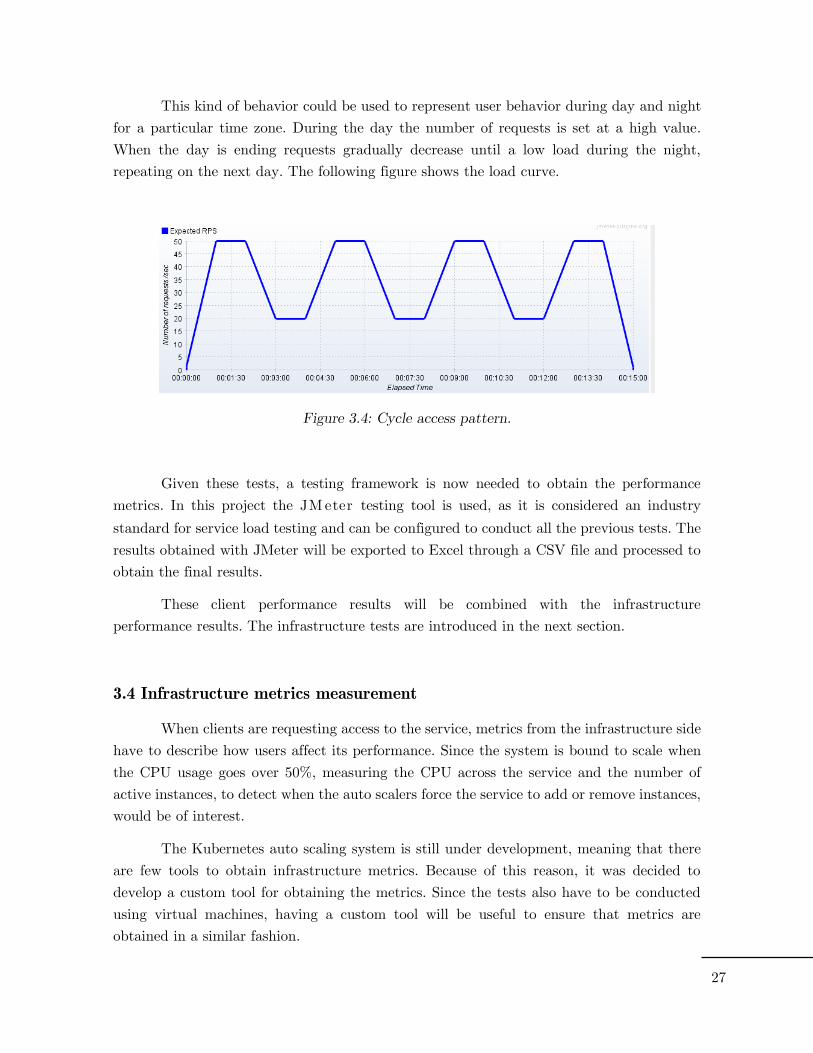
This kind of behavior could be used to represent user behavior during day and night
for a particular time zone. During the day the number of requests is set at a high value.
When the day is ending requests gradually decrease until a low load during the night,
repeating on the next day. The following figure shows the load curve.
Figure 3.4: Cycle access pattern.
Given these tests, a testing framework is now needed to obtain the performance
metrics. In this project the JM eter testing tool is used, as it is considered an industry
standard for service load testing and can be configured to conduct all the previous tests. The
results obtained with JMeter will be exported to Excel through a CSV file and processed to
obtain the final results.
These client performance results will be combined with the infrastructure
performance results. The infrastructure tests are introduced in the next section.
3.4 Infrastructure metrics measurement
When clients are requesting access to the service, metrics from the infrastructure side
have to describe how users affect its performance. Since the system is bound to scale when
the CPU usage goes over 50%, measuring the CPU across the service and the number of
active instances, to detect when the auto scalers force the service to add or remove instances,
would be of interest.
The Kubernetes auto scaling system is still under development, meaning that there
are few tools to obtain infrastructure metrics. Because of this reason, it was decided to
develop a custom tool for obtaining the metrics. Since the tests also have to be conducted
using virtual machines, having a custom tool will be useful to ensure that metrics are
obtained in a similar fashion.
27

Both Kubernetes and AWS expose their metrics through APIs, however since the
command line interfaces for both infrastructures are able to format their output as JSON
files, the metric tool will call the command line interfaces instead of directly accessing the
APIs.
Since WordPress uses MySQL as its database backend, analyzing how does its
performance affect the performance of the whole service could be of interest. To achieve this,
the CPU usage and memory consumption of the MySQL pod has to be monitored. However,
the Kubernetes command line does not expose this functionality. Instead, the REST API of
Heapster has to be used. Its API can be accessed through HTTP using the Kubernetes proxy,
obtaining in a simple way the needed metrics. The following diagram illustrates how does
the infrastructure metric measuring tool work.
Figure 3.5: Infrastructure metric measuring tool.
The source code for the infrastructure metric tool is available in the listing 3.3 at the
end of this document. The tool has been developed using Node.JS and JavaScript. With all
the environment and tests defined, and the metric measuring tools correctly set-up and
configured, the next chapter deals with the execution of the tests and shows the obtained
results.
28


Chapter 4
Tests
With the testing environment properly defined set-up, the performance evaluation can be
conducted. This chapter introduces the test bench used to execute the previously designed
tests, and the obtained results.
4.1 Test bench
The service was tested under three different virtual machine profiles with different
performance properties (under small virtual machines (t2.micro), medium (t2.small) and
large (t2.medium)). The Kubernetes cluster was formed by 5 instances, 5 minions and 1
master instance. The traditional virtual machine configuration started with 1 instance and
could scale up to 5 instances.
EC2 virtual machines use credits as the measurement unit for CPU performance.
One credit equals to a physical CPU being at 100% usage during one minute[Cred]. VM
instances get assigned a number of credits per hour (c / h), which roughly translate to the
equivalent time the CPU could be at 100% usage.
The following table shows the performance characteristics of each one of the testing
virtual machine profiles.
Small Medium Large
CPU speed 1 vCore * 3 c/h 1 vCore * 6 c/h 1 vCore * 12 c/h
Memory capacity 1 GiB 2 GiB 4 GiB
Storage type EBS (slow) EBS (slow) EBS (slow)
Network throughput Slow Slow Moderate
Table 4.1: Performance characteristics of the testing virtual machines.
The VM tests use the Bitnami WordPress AMI[Wp], which is a self-configuring image
of WordPress, and the Kubernetes tests use the default Kubernetes AMI, Debian 8[Deb].
30
4.2 Test results
After executing the tests in the three tiers, the following results were obtained. First
are the results on a small sized Kubernetes and small sized virtual machines, presenting first
the flood results, then the ramp results and finally the cycle results.
The horizontal axis represents the time stamp of each sample in minutes, while in
the vertical axis the mean response time is represented through the orange color and, in the
case of the container based test, the service average CPU usage is represented with the blue
color. Green horizontal bars are used to mark when the service scales horizontally, changing
the number of containers or virtual machines depending on the test. Samples are spaced
each 30 seconds approximately, taking 10 minutes the first two tests and 15 minutes the
third one.
After the results of the test for all three performance profiles have been introduced,
the economic cost of running each one of the alternatives is presented.
4.2.1 Small profile test results
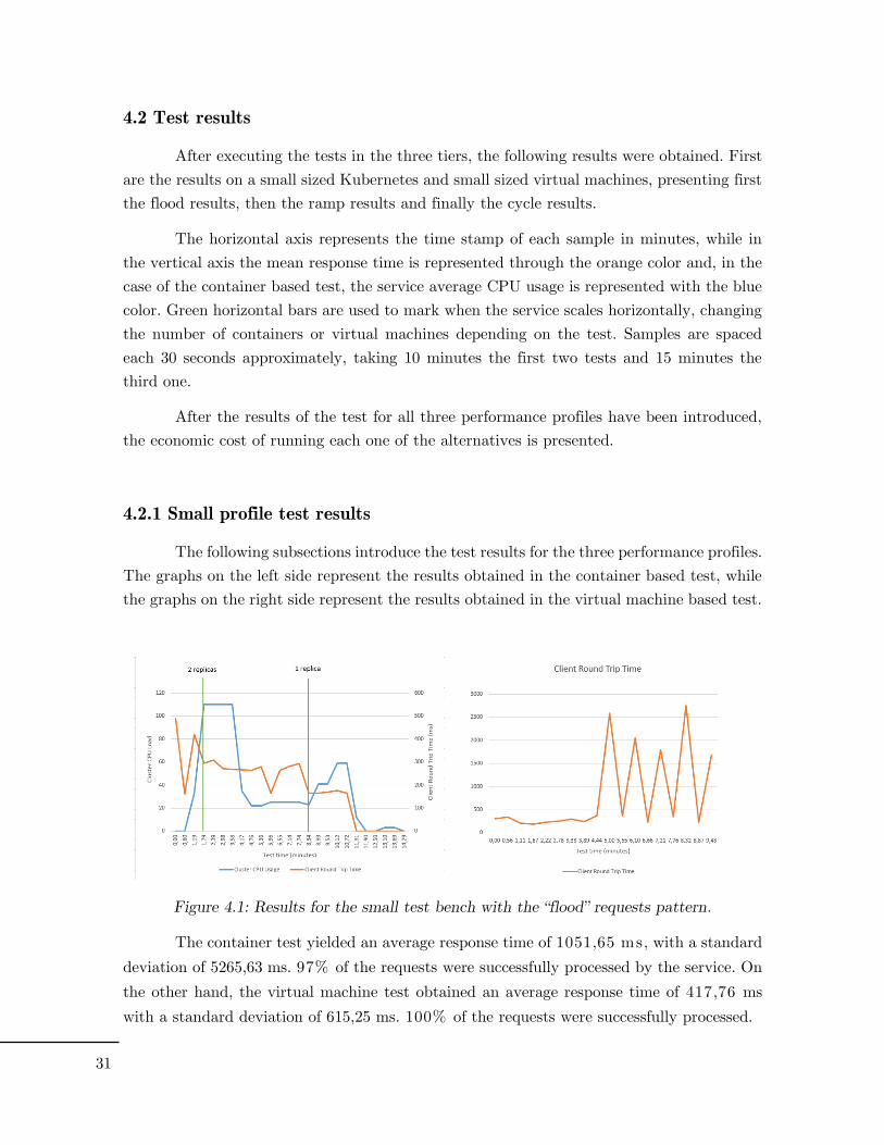
The following subsections introduce the test results for the three performance profiles.
The graphs on the left side represent the results obtained in the container based test, while
the graphs on the right side represent the results obtained in the virtual machine based test.
Figure 4.1: Results for the small test bench with the “flood” requests pattern.
The container test yielded an average response time of 1051,65 ms, with a standard
deviation of 5265,63 ms. 97% of the requests were successfully processed by the service. On
the other hand, the virtual machine test obtained an average response time of 417,76 ms
with a standard deviation of 615,25 ms. 100% of the requests were successfully processed.
31

The high round trip times, the occasional dropping of connections and the highly
variable response time in the virtual machine test could be symptoms of both tests failing
due to the small compute capacity of the machines.
The next figure shows the test results for the ramp test for both containers and
virtual machines.
Figure 4.2: Results for the small test bench with the “ramp” request pattern.
The mean response time for the container test was 834,23 ms, with a standard
deviation of 3796,17 ms. 96% of the requests completed successfully. The virtual machine
test obtained a mean response time of 220,43 ms with a standard deviation of 92,94 ms.
100% of the requests were handled correctly.
As with the previous case, the tests seem to be failing due to the machines being
underpowered to handle all the incoming requests. Finally, the following figure shows the
results of the cycle tests.
Figure 4.3: Results for the small test bench with the “cycle” requests pattern.
32

The container based test obtained a mean response time of 1505,70 ms with a
standard deviation of 5676,63 ms. 95% of the requests were processed. The virtual machine
test obtained a response time of 969,85 ms with a standard deviation of 1235,34 ms. 100%
of the requests were processed correctly.
In this case, similarly to the previous two, the excessively high and varying response
times could be caused to the inability of the machines to accept the load due to their reduced
computing capacity. In the case of the container test, The CPU load increases during the
first cycle and the cluster manages to scale up correctly. However, on the second cycle the
CPU load stays high and the response time increases significantly.
4.2.2 Medium profile test results
Next are the results for the medium performance characteristics. As with the small
tests, first are the results for the flood test.
Figure 4.4: Results for the medium test bench with the “flood” requests pattern.
The medium container based test obtained an average response time of 224,37 ms
with a standard deviation of 166,25 ms. 100% of the requests were handled in time. On the
other hand, the virtual machine based test obtained an average response time of 545,17 ms
with a standard deviation of 177,14 ms. 100% of the requests were handled successfully.
In this case, both tests completed successfully, with an acceptable response rate and
handling all the incoming connections. The container tests scaled to accommodate the
incoming requests, however it failed to scale down after the CPU load was correctly handled.
This could be an issue on the service HPA, since this Kubernetes feature is still under
development. On the other hand, the virtual machine test did not scale during the process.
Next is the ramp test for the medium performance profile.
33
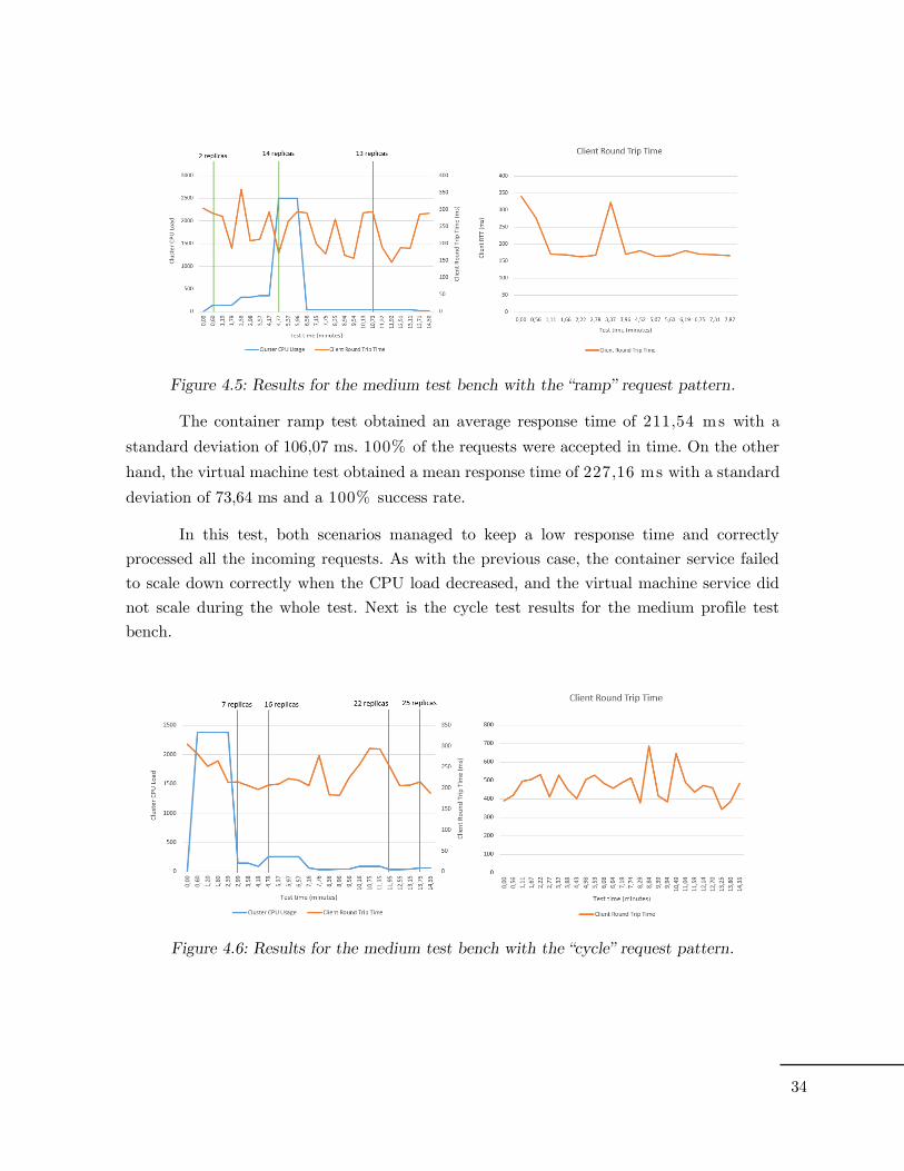
Figure 4.5: Results for the medium test bench with the “ramp” request pattern.
The container ramp test obtained an average response time of 211,54 ms with a
standard deviation of 106,07 ms. 100% of the requests were accepted in time. On the other
hand, the virtual machine test obtained a mean response time of 227,16 ms with a standard
deviation of 73,64 ms and a 100% success rate.
In this test, both scenarios managed to keep a low response time and correctly
processed all the incoming requests. As with the previous case, the container service failed
to scale down correctly when the CPU load decreased, and the virtual machine service did
not scale during the whole test. Next is the cycle test results for the medium profile test
bench.
Figure 4.6: Results for the medium test bench with the “cycle” request pattern.
34

The medium cycle container test obtained an average response time of 232,42 ms
with a standard deviation of 82,75 ms and a 100% success rate, while the virtual machine
test obtained an average response time of 541,34 ms with a standard deviation of 205,73
ms and a 100% success rate.
As with the previous tests, both scenarios completed successfully. Again, the
container cluster failed to scale down and the virtual machine service did not scale at all.
4.2.3 Large profile test results
Finally, the large profile tests results are introduced. As with the two previous
profiles, first are the flood test results.
Figure 4.7: Results for the large test bench with the “flood” request pattern.
The large container based test obtained an average response time of 208,17 ms with
a standard deviation of 87,90 ms. 100% of the requests were handled in time. On the other
hand, the virtual machine based test obtained an average response time of 303,11 ms with
a standard deviation of 79,48 ms. 100% of the requests were handled successfully.
In this case both scenarios completed successfully. Given the unusually high CPU
load of the container cluster, it might be due to the HPA not being able to retrieve the CPU
load of each pod correctly, producing a wrong result. Next is the ramp test for the large
performance profile.
35

Figure 4.8: Ramp results for the large test bench.
The container ramp test obtained an average response time of 193,65 ms with a
standard deviation of 77,36 ms. 100% of the requests were accepted in time. On the other
hand, the virtual machine test obtained a mean response time of 188,77 ms with a standard
deviation of 57,82 ms and a 100% success rate. Next is the cycle test results for the large
profile test bench.
Like the previous large profile test, both scenarios completed successfully. In this
case, the container cluster failed to scale up in time, with the CPU load being over the
maximum threshold during 3/4ths of the test.
Figure 4.9: Cycle results for the large test bench.
The large cycle container test obtained an average response time of 232,42 ms with
a standard deviation of 82,75 ms and a 100% success rate, while the virtual machine test
obtained an average response time of 253,45 ms with a standard deviation of 78,71 ms and
a 100% success rate.
36

Like the two previous tests, both scenarios completed successfully. Again, the
container cluster seems to have failed at gathering the correct CPU usage information, as
well as failing to scale up and down when required.
4.3 Results discussion
The main objective of this project is assessing if there is a benefit on using container
management systems instead of traditional virtual machines for distributed systems. Given
the performance results, it is clear that when used on small profile machines, the container
based service cannot keep up with the client load in none of the tests, while the virtual
machine based approach does keep up when tested against the ramp request pattern. This
could be explained by the overhead introduced by Kubernetes, which may require more
computing performance than the available in the small sized cluster.
However, in the medium and large clusters both container and virtual machine based
services handle the client requests in appropriate time, dropping no connections in the
process. The medium profile tests present several latency spikes, but in most cases the results
are inside the expected values.
From these two later test profiles, it can be seen how the container based approach
features a shorter response time in average, thus giving users a better experience. Then,
taking into account only the computing performance of each alternative, using containers
seems a better solution.
Even though the virtual machine based service was bound to scale up when the CPU
load exceeded 50%, this did not happen in any of the tests, completing with a single instance
in all cases.
The economic cost of running the needed virtual machines adds more considerations
to take into account in order to make a decision. Even though the container based solutions
offer better performance and could improve the overall user experience, running the smallest
sized cluster has a cost in par with running only one of the largest virtual machines.
For this reason, it could be necessary to verify whether the workloads used by the
service provider require the flexibility and fast scalability properties of container
management systems or if using bare virtual machines make up for their needs.
37
4.4 Cost evaluation
Another concern with the container based approach is the economic cost associated
with running a whole cluster instead of a single or several virtual machines. In cases when
the container management system cluster and the traditional virtual machine cluster share
the same number of instances, this would not be a problem, but in cases where one single
virtual machine performs similarly to a whole container cluster, it might suppose spending
unnecessary money.
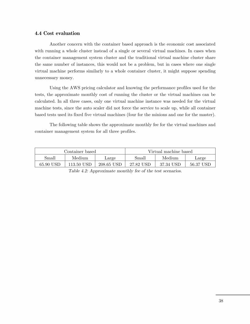
Using the AWS pricing calculator and knowing the performance profiles used for the
tests, the approximate monthly cost of running the cluster or the virtual machines can be
calculated. In all three cases, only one virtual machine instance was needed for the virtual
machine tests, since the auto scaler did not force the service to scale up, while all container
based tests used its fixed five virtual machines (four for the minions and one for the master).
The following table shows the approximate monthly fee for the virtual machines and
container management system for all three profiles.
Container based Virtual machine based
Small Medium Large Small Medium Large
65.90 USD 113.50 USD 208.65 USD 27.82 USD 37.34 USD 56.37 USD
Table 4.2: Approximate monthly fee of the test scenarios.
38


Chapter 5
Conclusions
The results from the tests prove that container management systems can improve the
performance of distributed applications when compared to traditional virtual machines, if
the underlying system is able to support the overhead added by the management system.
Even though from a purely technical standpoint using a container management
system could translate into a better user experience and thus better results for the service,
in practice the cost of running and operating the container management system must be
taken into account.
Not only the usage of a container management system could be potentially more
expensive than using virtual machines, but the additional training that developers and
system operators must do before being able to use these systems should also be taken into
account. To tackle this problem, major public cloud providers have created their own
container management systems, such as Amazon Elastic Container Service or Google’s
Compute Engine, offering the flexibility of containers without the complexities of
maintaining a dedicated container cluster.
This project is a good example of the previous statement: using Kubernetes has
implied a long training time to properly understand its inner workings and its possibilities
before being able to conduct the tests.
In conclusion, from a practical standpoint the usage of container management
systems should be a matter of how useful is it for the developer workloads, taking into
account economical cost and the required target performance.
5.1 Future work
Since the project had to be completed in a short time span, there is plenty of room for
improvement. Following are several objectives that could contribute to the project’s future
work:
40

Testing the application on different virtual machine performance profiles, such as
AWS’s large or extra-large machines, and on VM’s specialized in high throughput
applications, such as distributed services.
Conducting tests with different access patterns, on longer periods and with varying
user loads over time.
Testing the performance of a container management system with more than a single
service running on it. In a typical real life scenario, service developers might want to
take profit of the container management system to deploy more than one service in
a single cluster.
Using different cloud providers, such as Microsoft Azure, IBM SoftLayer or a private
cloud provider like OpenStack or OpenNebula, to see how can the performance of
the virtual machine hypervisors and network devices on each cloud service affect the
overall performance of the container cluster.
Testing the container workloads on dedicated cloud container management systems,
such as Google Compute Engine or Amazon ECS, to check the difference between
running container workloads on a self-deployed and self-managed cluster and running
them on a highly tested and proven platform.
41

References
[Felter15] An updated performance comparison of virtual machines and Linux containers,
Wes Felter; IBM Research, Austin, TX ; Alexandre Ferreira ; Ram Rajamony; Juan
Rubio (2015), Performance Analysis of Systems and Software (ISPASS).
[Ann15] Performance comparison between Linux containers and virtual machines, Ann
Mary Joy (2015), Computer Engineering and Applications (ICACEA).
[Mell11] The NIST definition of cloud computing, P. Mell, T. Grance (2011), The National
Institute of Standards and Technology (NIST).
[Meier07] Performance Testing Guidance for Web Applications, D. Meier, Carlos Farre,
Prashant Bansode, Scott Barber, Dennis Rea (2007), Microsoft Corporation.
[Adler99] The Slashdot effect: an analysis of three Internet publications, S. Adler (1999),
Linux Gazette.
[Berman03] Grid computing: making the global infrastructure a reality, F. Berman, G.
Fox, AJG. Hey (2003).
[Merkel04] Docker: lightweight Linux containers for consistent development and
deployment, D. Merkel (2014), Linux Journal.
[Nova] Nova-Docker: Docker driver for OpenStack (https://github.com/openstack/nova-
docker, active September 15th 2016).
[Dock] OneDock: Docker suport for OpenNebula, by Indigo-DataCloud
(https://github.com/indigo-dc/onedock, active September 15th 2016).
[Graf] Grafana, by Torkel Ödegaard & Coding Instinct AB, 2015 (http://grafana.org/,
active September 15th 2016).
[Heap] Heapster: Container Cluster Monitoring and Performance Analysis for Kubernetes.
(https://github.com/kubernetes/heapster, active September 15th 2016).
[Deb] Debian 8 AWS AMI (https://aws.amazon.com/marketplace/pp/B00WUNJIEE,
active September 15th 2016).
[Wp] Wordpress by Bitnami AWS AMI
(https://aws.amazon.com/marketplace/pp/B007IP8BKQ?qid=1474047636447, active
September 15th 2016).
42

Kubernetes Reference by Google Inc. (http://kubernetes.io/docs/reference/, active
September 15th 2016).
Kubernetes Cookbook, Ke-Jou Carol Hsu, Hui-Chuan Chloe Lee, Hideto Saito (2016),
Packt Publishing.
Getting Started with Kubernetes, Jonathan Baier (2016), Packt Publishing.
Heapster REST API by Google Inc.
(https://github.com/kubernetes/heapster/blob/master/docs/model.md, active September
15th 2016).
JMeter User Manual, by the Apache Foundation
(http://jmeter.apache.org/usermanual/index.html, active September 15th 2016).
43

Annexes
Listing 3.1: YAML description for the WordPress service.
apiVersion: v1
kind: ReplicationController metadata: name: wordpress spec: replicas: 1 selector: app: wordpress template: metadata: name: wordpress labels: app: wordpress spec: containers: - name: wordpress image: wordpress env: - name: WORDPRESS_DB_PASSWORD value: tfm2016 - name: WORDPRESS_DB_HOST value: mysqlservice:3306 ports: - containerPort: 80 --- apiVersion: v1 kind: Service metadata: labels: name: wpservice name: wpservice spec: ports: - port: 80 selector: app: wordpress type: LoadBalancer --- apiVersion: extensions/v1beta1 kind: HorizontalPodAutoscaler metadata: name: wphpa namespace: default spec: scaleRef: kind: ReplicationController name: wordpress subresource: scale minReplicas: 1 maxReplicas: 50 cpuUtilization: targetPercentage: 50
44

Listing 3.2: YAML description for the MySQL service.
apiVersion: v1
kind: Pod metadata: name: mysql labels: name: mysql spec: containers: - image: mysql:5.6 name: mysql env: - name: MYSQL_ROOT_PASSWORD value: tfm2016 ports: - containerPort: 3306 name: mysql --- apiVersion: v1 kind: Service metadata: labels: name: mysqlservice name: mysqlservice spec: ports: - port: 3306 selector: name: mysql
Listing 3.3: Source code for the infrastructure metric tool.
// César González Segura, 2016 // Imports const fs = require("fs"); const execSync = require("child_process").execSync;
// Global variables var settings = null; var data = null; const settingsPath = "./config.json";
function main() { // Read the logger settings settings = JSON.parse(fs.readFileSync(settingsPath)); // Set the data update interval setInterval(onUpdateData, settings.updateInterval * 1000); // Set the saving update interval setInterval(onSaveData, settings.saveInterval * 1000); // Initialize the data data = { "updateRate": settings.updateInterval, "maxReplicas": 0, "minReplicas": 0, "targetCpu": 0, "timeStamp": new Array(), "currentInstances": new Array(),
45

"desiredInstances" : new Array(), "cpuLoad": new Array(), "mysqlMemUsage": new Array(), "mysqlCpuUsage": new Array() }; }
function saveData(fn, fmt) { if (fmt == "dlm") { // Save the const settings as a separate dlm file // if it doesn't exist var constFn = "hpa_const.dlm"; try { fs.statSync(constFn); } catch (e) { var dt = data.updateRate + " " + data.maxReplicas + " " + data.minReplicas + " " + data.targetCpu; fs.writeFileSync(constFn, dt); } // Save the logged data as a dlm matrix // Column format: // | Time | CurrentInstances | DesiredInstances | CPULoad | var dt = ""; for (var i = 0; i < data.timeStamp.length; i++) { dt += data.timeStamp[i].getTime().toString() + " " + data.currentInstances[i] + " " + data.desiredInstances[i] + " " + data.cpuLoad[i] + " " + data.mysqlMemUsage[i] + " " + data.mysqlCpuUsage[i] + "\n"; } fs.writeFileSync(fn, dt); } else if (fmt == "json") { fs.writeFileSync(fn, JSON.stringify(data)); } }
function onUpdateData() { if (settings.verbose) { console.log("[UPDATE] Logging new data from Kubernetes cluster..."); } // Attempt to run kubectl to retrieve the HPA status var result = execSync("kubectl get hpa " + settings.hpaName + " -o json"); var jr = JSON.parse(result.toString()); // Add timestamp data.timeStamp.push(new Date()); // Add current instance count data.currentInstances.push(jr.status.currentReplicas); // Add desired instance count data.desiredInstances.push(jr.status.desiredReplicas);
46

// Add current CPU load data.cpuLoad.push(jr.status.currentCPUUtilizationPercentage); // Update the const settings data.maxReplicas = jr.spec.maxReplicas; data.minReplicas = jr.spec.minReplicas; data.targetCpu = jr.spec.targetCPUUtilizationPercentage; // Request to Heapster the MySQL pod current memory usage var mem = requestMysqlMemoryUsage(); data.mysqlMemUsage.push(mem); // Request the MySQL CPU usage var cpu = requestMysqlCpuUsage(); data.mysqlCpuUsage.push(cpu); if (settings.verbose) { console.log("[UPDATE] HPA status (" + data.timeStamp[data.timeStamp.length - 1].toISOString() + "):"); console.log("[UPDATE] Current replicas: " + data.currentInstances[data.currentInstances.length - 1]); console.log("[UPDATE] Desired replicas: " + data.desiredInstances[data.desiredInstances.length - 1]); console.log("[UPDATE] Current CPU load: " + data.cpuLoad[data.cpuLoad.length - 1]); console.log("[UPDATE] Current MySQL status: " + cpu + "% / " + mem / 1000000.0 + " MB"); } }
function requestMysqlMemoryUsage() { var url = "https://" + settings.kubeAddr + "/api/v1/proxy/namespaces/kube-system/services/heapster/api/v1/model/namespaces/default/pods/" + settings.mysqlPodName + "/metrics/memory/usage"; var result = execSync("curl -k -u admin:" + settings.kubePass + " " + url); var jr = JSON.parse(result.toString()); return jr.metrics[jr.metrics.length - 1].value; }
function requestMysqlCpuUsage() { var url = "https://" + settings.kubeAddr + "/api/v1/proxy/namespaces/kube-system/services/heapster/api/v1/model/namespaces/default/pods/" + settings.mysqlPodName + "/metrics/cpu/usage_rate"; var result = execSync("curl -k -u admin:" + settings.kubePass + " " + url); var jr = JSON.parse(result.toString()); return jr.metrics[jr.metrics.length - 1].value; }
function onSaveData() { var fileName = settings.output; // Check if there are any macros in the // filename if (fileName.indexOf("[date]") != -1) { fileName = fileName.replace("[date]", (new Date()).toISOString()); } // Append the format extension
47

fileName += "." + settings.format; // Use the appropriate method depending on the // output format saveData(fileName, settings.format); if (settings.verbose) { console.log("[SAVE] Saved result to " + fileName); } }
main();
Configuration file for the testing program (config.json):
{ "updateInterval": 30, "saveInterval": 300, "format": "dlm", "hpaName": "wphpa", "mysqlPodName": "mysql", "output": "hpa_[date]", "kubeAddr": "KubernetesMasterIPAddress", "kubePass": "KubernetesProxyHTTPSPassword", "verbose": true }
48