analysis of human voice production using inverse …lib.tkk.fi/dipl/2005/urn007925.pdfhelsinki...
TRANSCRIPT

HELSINKI UNIVERSITY OF TECHNOLOGYDepartment of Computer Science and Engineering
Hannu Pulakka
Analysis of Human Voice Production UsingInverse Filtering, High-Speed Imaging, andElectroglottography
Master’s Thesis submitted in partial fulfillment of the requirements for the degree ofMaster of Science in Technology.
Espoo, 14 February 2005
Supervisor: Professor Paavo Alku

HELSINKI UNIVERSITY OF TECHNOLOGY ABSTRACT OF MASTER’S THESISDepartment of Computer Science and Engineering
Author: Hannu Pulakka Date: 14 February 2005Pages: 104 + 7
Title of thesis: Analysis of Human Voice Production Using Inverse Filtering, High-SpeedImaging, and Electroglottography
Professorship: Language technology Professorship code: S-89
Supervisor: Professor Paavo Alku
Instructor: Professor Paavo Alku
Human voice production was studied using three methods: inverse filtering, digital high-speedimaging of the vocal folds, and electroglottography. The primary goal was to evaluate an inversefiltering method by comparing inverse filtered glottal flow estimates with information obtainedby the other methods. More detailed examination of the human voice source behavior was alsoincluded in the work.
Material from two experiments was analyzed in this study. The data of the first experimentconsisted of simultaneous recordings of acoustic speech signal, electroglottogram, and high-speedimaging acquired during sustained vowel phonations. Inverse filtered glottal flow estimates werecompared with glottal area waveforms derived from the image material by calculating pulseshape parameters from the signals. The material of the second experiment included recordings ofacoustic speech signal and electroglottogram during phonations of sustained vowels. This mate-rial was utilized for the analysis of the opening phase and the closing phase of vocal fold vibration.
The evaluated inverse filtering method was found to produce mostly reasonable estimatesof glottal flow. However, the parameters of the system have to be set appropriately, whichrequires experience on inverse filtering and speech production. The flow estimates often showed atwo-stage opening phase with two instants of rapid increase in the flow derivative. The instant ofglottal opening detected in the electroglottogram was often found to coincide with an increase inthe flow derivative. The instant of minimum flow derivative was found to occur mostly during thelast quarter of the closing phase and it was shown to precede the closing peak of the differentiatedelectroglottogram.
Keywords: speech production, glottal flow, vocal fold vibration, digital high-speed imaging,inverse filtering, electroglottography
i

TEKNILLINEN KORKEAKOULU DIPLOMITYÖN TIIVISTELMÄTietotekniikan osasto
Tekijä: Hannu Pulakka Päiväys: 14.2.2005Sivumäärä: 104 + 7
Työn nimi: Ihmisen äänentuoton analysointi käänteissuodatuksen, suurnopeuskuvauksenja elektroglottografian avulla
Professuuri: Kieliteknologia Koodi: S-89
Työn valvoja: professori Paavo Alku
Työn ohjaaja: professori Paavo Alku
Ihmisen puheentuottoa tutkittiin kolmella menetelmällä: käänteissuodatuksella, äänihuultendigitaalisella suurnopeuskuvauksella ja elektroglottografialla. Päätavoitteena oli tarkastella eräänkäänteissuodatusmenetelmän toimintaa vertailemalla näillä menetelmillä saatua informaatiotaäänihuulten värähtelystä. Lisäksi tutkittiin tarkemmin eräitä äänilähteen käyttäytymisen yksityis-kohtia.
Tutkimuksessa analysoitiin aineistoa kahdesta koejärjestelystä. Ensimmäisessä kokeessatallennettiin samanaikaisesti äänisignaali, elektroglottogrammi ja suurnopeuskuvamateriaaliaäänihuulista koehenkilöiden tuottaessa pitkiä vokaaleita. Käänteissuodatuksella saaduista glot-tisvirtausestimaateista sekä kuvamateriaalin ilmaisemasta ääniraon pinta-alavaihtelusta laskettiinpulssiparametreja, joiden avulla vertailtiin virtauksen ja ääniraon pinta-alan käyttäytymistä.Toisen koejärjestelyn aineisto koostui äänisignaalista ja elektroglottogrammista, jotka oli tallen-nettu vokaaliääntöjen aikana. Tämän materiaalin perusteella analysoitiin ääniraon avautumis- jasulkeutumisvaihetta.
Tarkastellun käänteissuodatusmenetelmän todettiin tuottavan enimmäkseen luotettavia vir-tausestimaatteja edellyttäen, että menetelmän parametrit asetetaan tarkoituksenmukaisesti, mikävaatii käyttäjältä kokemusta käänteissuodatuksesta ja ihmisen puheentuotosta. Glottisvirtauksenavautumisvaiheen havaittiin olevan useissa virtausestimaateissa kaksivaiheinen siten, että vir-tauksen kasvu voimistuu nopeasti kahdessa kohdassa sulkeutumisen ja maksimivirtauksen välillä.Virtauksen kasvun todettiin usein voimistuvan elektroglottogrammista tunnistetun ääniraon avau-tumishetken lähellä. Virtauksen derivaatan minimikohdan havaittiin sijoittuvan enimmäkseenvirtauksen sulkeutumisvaiheen viimeiseen neljännekseen, ja sen osoitettiin esiintyvän ennenelektroglottogrammin derivaatan minimikohtaa.
Avainsanat: puheentuotto, glottisvirtaus, äänihuulten värähtely, digitaalinen suurnopeuskuvaus,käänteissuodatus, elektroglottografia
ii

Acknowledgements
This Master’s thesis was carrier out in the Laboratory of Acoustics and Audio SignalProcessing and Helsinki University of Technology. The research was supported by theAcademy of Finland (project no. 205962).
In the first place, I want to thank my supervisor professor Paavo Alku for providing me thepossibility to do my Master’s thesis on this interesting topic. His professional knowledgeand ideas as well as the encouraging feedback from him have been essential in this work.
I am also grateful to Svante Granqvist and Hans Larsson from KTH and the HuddingeUniversity Hospital of the Karolinska Institute in Stockholm, Stellan Hertegård and Per-Åke Lindestad from the Huddinge University Hospital, Anne-Maria Laukkanen from theUniversity of Tampere, Erkki Vilkman from the Helsinki University Central Hospital, andPaavo Alku, who carried out the data recording session at the Huddinge University Hospital.Especially, I want to thank Svante Granqvist for answering numerous technical questionsregarding the material that was analyzed in this study. Svante Granqvist and Hans Larssonalso allowed me to use computer programs they had developed for the analysis of high-speed image recordings.
Finally, I would like to thank Matti Airas for technical support and valuable commentson the work, Eva Björkner and Laura Lehto for their contribution, and Juho Kontio forproposing improvements to several graphical illustrations.
Otaniemi, 14 February 2005
Hannu Pulakka
iii

Contents
Abbreviations vii
List of Figures x
List of Tables xi
1 Introduction 1
1.1 Background . . . . . . . . . . . . . . . . . . . . . . . . . . . . . . . . . . 1
1.2 Structure of the Thesis . . . . . . . . . . . . . . . . . . . . . . . . . . . . 2
2 Physiological and Theoretical Background 4
2.1 Physiology of Voice Production . . . . . . . . . . . . . . . . . . . . . . . 4
2.1.1 Vocal Folds . . . . . . . . . . . . . . . . . . . . . . . . . . . . . . 4
2.1.2 Vocal Tract . . . . . . . . . . . . . . . . . . . . . . . . . . . . . . 7
2.1.3 Registers and Phonation Modes . . . . . . . . . . . . . . . . . . . 7
2.2 Source-Filter Theory . . . . . . . . . . . . . . . . . . . . . . . . . . . . . 8
3 Analysis Methods 11
3.1 Inverse Filtering . . . . . . . . . . . . . . . . . . . . . . . . . . . . . . . . 11
3.2 Videostroboscopy and Videokymography . . . . . . . . . . . . . . . . . . 13
3.3 High-Speed Imaging . . . . . . . . . . . . . . . . . . . . . . . . . . . . . 15
3.3.1 Detection of Vocal Fold Edges and Glottal Area . . . . . . . . . . . 16
3.4 Electroglottography . . . . . . . . . . . . . . . . . . . . . . . . . . . . . . 17
iv

3.5 Other Analysis Methods . . . . . . . . . . . . . . . . . . . . . . . . . . . 20
3.6 Studies Combining Several Analysis Methods . . . . . . . . . . . . . . . . 21
3.7 Parametrization of Glottal Flow and Area . . . . . . . . . . . . . . . . . . 22
4 Material and Methods 26
4.1 Matlab Signal Processing and Programming Environment . . . . . . . . . . 26
4.2 Iterative Adaptive Inverse Filtering (IAIF) . . . . . . . . . . . . . . . . . . 26
4.2.1 HUT IAIF Toolbox . . . . . . . . . . . . . . . . . . . . . . . . . . 29
4.3 Huddinge Experiment . . . . . . . . . . . . . . . . . . . . . . . . . . . . . 30
4.3.1 Recording Setup . . . . . . . . . . . . . . . . . . . . . . . . . . . 30
4.3.2 Data Selection and Preprocessing . . . . . . . . . . . . . . . . . . 34
4.3.3 Calculation of the Sound Pressure Level . . . . . . . . . . . . . . . 35
4.3.4 Inverse Filtering . . . . . . . . . . . . . . . . . . . . . . . . . . . 37
4.3.5 Glottal Area Function . . . . . . . . . . . . . . . . . . . . . . . . 38
4.3.6 Error Estimates of Individual Pulse Parameters . . . . . . . . . . . 43
4.3.7 Synchronization . . . . . . . . . . . . . . . . . . . . . . . . . . . 48
4.4 HUT Experiment . . . . . . . . . . . . . . . . . . . . . . . . . . . . . . . 55
4.4.1 Recording Setup . . . . . . . . . . . . . . . . . . . . . . . . . . . 55
4.4.2 Data Selection and Preprocessing . . . . . . . . . . . . . . . . . . 55
4.4.3 Calculation of the Sound Pressure Level . . . . . . . . . . . . . . . 56
4.4.4 Inverse Filtering . . . . . . . . . . . . . . . . . . . . . . . . . . . 56
4.4.5 Electroglottogram . . . . . . . . . . . . . . . . . . . . . . . . . . 56
4.4.6 Compensation of the Propagation Delay . . . . . . . . . . . . . . . 56
4.4.7 Parametrization of Glottal Flow and EGG . . . . . . . . . . . . . . 57
5 Results 61
5.1 Huddinge Experiment . . . . . . . . . . . . . . . . . . . . . . . . . . . . . 61
5.1.1 Sound Pressure Level Estimates . . . . . . . . . . . . . . . . . . . 61
5.1.2 Qualitative Observations . . . . . . . . . . . . . . . . . . . . . . . 66
5.1.3 Pulse Parameters . . . . . . . . . . . . . . . . . . . . . . . . . . . 68
v

5.1.4 Mean Pulse Parameters . . . . . . . . . . . . . . . . . . . . . . . . 69
5.2 HUT Experiment . . . . . . . . . . . . . . . . . . . . . . . . . . . . . . . 73
5.2.1 Sound Pressure Level Estimates . . . . . . . . . . . . . . . . . . . 73
5.2.2 Opening Phase . . . . . . . . . . . . . . . . . . . . . . . . . . . . 75
5.2.3 Closing Phase . . . . . . . . . . . . . . . . . . . . . . . . . . . . . 78
5.3 Observations on Inverse Filtering . . . . . . . . . . . . . . . . . . . . . . . 83
5.3.1 Primary and Secondary Opening . . . . . . . . . . . . . . . . . . . 83
6 Conclusions 89
6.1 Conclusions about the Inverse Filtering Method . . . . . . . . . . . . . . . 89
6.2 Detailed Observations . . . . . . . . . . . . . . . . . . . . . . . . . . . . . 90
6.2.1 Incomplete Closure of Vocal Folds . . . . . . . . . . . . . . . . . . 90
6.2.2 Pulse Skewing . . . . . . . . . . . . . . . . . . . . . . . . . . . . 90
6.2.3 Flow Waveform in the Closed Phase and the Opening Phase . . . . 90
6.2.4 Closing Phase Phenomena . . . . . . . . . . . . . . . . . . . . . . 91
6.3 Sources of Error and Uncertainty . . . . . . . . . . . . . . . . . . . . . . . 92
6.3.1 Signal Synchronization . . . . . . . . . . . . . . . . . . . . . . . . 92
6.3.2 Estimation of Glottal Area . . . . . . . . . . . . . . . . . . . . . . 93
6.3.3 Time Resolution of High-Speed Image Sequences . . . . . . . . . . 93
6.3.4 Estimation of Pulse Parameters . . . . . . . . . . . . . . . . . . . 94
6.3.5 Suggestions for Technical Improvements . . . . . . . . . . . . . . 95
6.4 Concluding Remarks . . . . . . . . . . . . . . . . . . . . . . . . . . . . . 95
A Huddinge Data 105
vi

Abbreviations
ClQ Closing quotient (glottal pulse shape parameter)DAP Discrete all-pole modelingDAT Digital audio tapeDC Direct currentDEGG Differentiated electroglottogramEGG Electroglottography, electroglottogramEMGG Electromagnetic glottographyFFT Fast Fourier transformFGG Flow glottogramFM Frequency modulationGCI Glottal closure instantHUT Helsinki University of TechnologyIAIF Iterative adaptive inverse filteringLPC Linear predictive codingNAQ Normalized amplitude quotientOQ Open quotientPGG PhotoglottographySEM Standard error of the meanSPL Sound pressure levelSQ Speed quotient
vii
List of Figures
2.1 The human speech production mechanism . . . . . . . . . . . . . . . . . . 5
2.2 The larynx during respiration and phonation . . . . . . . . . . . . . . . . . 6
2.3 Cross profile of an idealized cycle of vocal fold vibration . . . . . . . . . . 7
2.4 Larynx in breathy, normal, and pressed phonation . . . . . . . . . . . . . . 8
2.5 Source-filter model . . . . . . . . . . . . . . . . . . . . . . . . . . . . . . 9
2.6 The components of the source-filter model in the frequency domain . . . . 10
3.1 Speech waveform and inverse filtered flow waveform . . . . . . . . . . . . 13
3.2 Simplified diagram of vocal fold imaging with a solid endoscope . . . . . . 14
3.3 Kymogram displaying the vibration of the vocal folds along a single line . . 15
3.4 EGG measurement setting . . . . . . . . . . . . . . . . . . . . . . . . . . 18
3.5 Electroglottogram of the normal phonation of a male subject . . . . . . . . 19
3.6 The phases of the EGG signal period according to the Rothenberg model . . 20
3.7 Schematic diagram of flow pulse phases . . . . . . . . . . . . . . . . . . . 22
3.8 Pulse parameters . . . . . . . . . . . . . . . . . . . . . . . . . . . . . . . 24
4.1 Block diagram of the steps of the IAIF method . . . . . . . . . . . . . . . 27
4.2 The graphical user interface of HUT IAIF Toolbox . . . . . . . . . . . . . 30
4.3 The signals window of HUT IAIF Toolbox . . . . . . . . . . . . . . . . . . 31
4.4 The Weinberger high-speed camera with the endoscope attached . . . . . . 33
4.5 Three-channel recording of breathy, normal, and pressed phonation . . . . . 34
4.6 Example of a noisy EGG signal . . . . . . . . . . . . . . . . . . . . . . . . 34
viii

4.7 Flow pulse with primary and secondary opening . . . . . . . . . . . . . . . 38
4.8 The High-Speed Toolbox software . . . . . . . . . . . . . . . . . . . . . . 39
4.9 Anterior and posterior chink . . . . . . . . . . . . . . . . . . . . . . . . . 41
4.10 Partially hidden glottis in pressed phonation . . . . . . . . . . . . . . . . . 41
4.11 Phases of a glottal area pulse . . . . . . . . . . . . . . . . . . . . . . . . . 43
4.12 Pulse waveform with closure, opening and maximum instants indicated . . 45
4.13 Video signal on the synchronization channel . . . . . . . . . . . . . . . . . 50
4.14 Evaluation of signal synchronization . . . . . . . . . . . . . . . . . . . . . 54
4.15 Mask for calculating the smoothed second derivative . . . . . . . . . . . . 58
4.16 Significant instants detected from the glottal flow waveform . . . . . . . . 58
4.17 Glottal closure and opening detected from the EGG waveform . . . . . . . 60
5.1 Huddinge SPL estimates, phonation types . . . . . . . . . . . . . . . . . . 64
5.2 Huddinge SPL estimates, loudness variation . . . . . . . . . . . . . . . . . 65
5.3 Phonation Male1-06-normal . . . . . . . . . . . . . . . . . . . . . . . . . 66
5.4 Phonation Male2-12-breathy . . . . . . . . . . . . . . . . . . . . . . . . . 67
5.5 Parameters of the phonations of Male 1 at normal loudness . . . . . . . . . 68
5.6 Pulse parameters of breathy, normal, and pressed phonations . . . . . . . . 71
5.7 Pulse parameters of phonations in different loudness categories . . . . . . . 72
5.8 SPL estimates of the HUT experiment . . . . . . . . . . . . . . . . . . . . 74
5.9 Illustration of the notation used in the examination of the opening phase . . 75
5.10 Significant instants detected from each glottal cycle . . . . . . . . . . . . . 77
5.11 Time scale of the closing phase . . . . . . . . . . . . . . . . . . . . . . . . 78
5.12 Positions of minima in flow derivative and closing peaks in DEGG . . . . . 79
5.13 Position of the minimum flow derivative . . . . . . . . . . . . . . . . . . . 80
5.14 Time difference between the closing peaks in differentiated flow and DEGG 81
5.15 Time difference between the closing instants in flow and EGG (ms) . . . . 81
5.16 Time difference between the closing instants in flow and EGG (normalized) 82
5.17 Comparison of inverse filtering methods . . . . . . . . . . . . . . . . . . . 84
ix

5.18 Flow waveforms obtained with two different lip radiation coefficients . . . 85
5.19 Two different flow waveforms obtained from the same pressure signal . . . 86
5.20 Problematic signal segment for inverse filtering . . . . . . . . . . . . . . . 88
A.1 Parameters of breathy, normal, and pressed phonation of Male 1 . . . . . . 106
A.2 Parameters of breathy, normal, and pressed phonation of Male 2 . . . . . . 107
A.3 Parameters of breathy, normal, and pressed phonation of Female 1 . . . . . 108
A.4 Parameters of soft, normal, and loud phonation of Male 1 . . . . . . . . . . 109
A.5 Parameters of soft, normal, and loud phonation of Male 2 . . . . . . . . . . 110
A.6 Parameters of soft, normal, and loud phonation of Female 1 . . . . . . . . . 111
x

List of Tables
5.1 Huddinge recordings . . . . . . . . . . . . . . . . . . . . . . . . . . . . . 62
5.2 SPL estimates of the Huddinge experiment, phonation types . . . . . . . . 63
5.3 SPL estimates of the Huddinge experiment, loudness variation . . . . . . . 63
5.4 Phonations selected for parameter analysis . . . . . . . . . . . . . . . . . . 69
5.5 SPL estimates of the HUT experiment . . . . . . . . . . . . . . . . . . . . 73
5.6 P values obtained from the t-test . . . . . . . . . . . . . . . . . . . . . . . 82
xi
Chapter 1
Introduction
1.1 Background
The vocal folds are located in the larynx and they are an essential part of the human speechmechanism. During speech, the vibration of the vocal folds converts the air flow from thelungs into a sequence of short flow pulses. This pulse train, the glottal flow, provides theexcitation signal of voiced speech sounds.
The vocal fold vibration cannot be directly measured with non-invasive methods becausethe larynx is not accessible during phonation. However, there are several indirect meansof studying the function of the vocal folds. One of the methods is called inverse filtering,which is used to estimate the pulsating air flow produced by the vibrating vocal folds. At aminimum, only the speech signal captured with a microphone is required for the procedure.Electroglottography is another voice analysis method. It measures impedance variationsacross the neck of the subject during speech. This yields information about vocal foldvibration because the varying amount of contact between the vocal folds causes impedancefluctuation. Inverse filtering and electroglottography are non-invasive methods: they do notrequire surgery or internal examination of the body, nor do they prevent the subject fromspeaking normally.
High-speed video recording of the larynx provides visual information about the move-ments of vocal folds. It is, however, more invasive than inverse filtering and electroglot-tography because an endoscope has to be inserted into the nasal or the oral cavity of thesubject. The endoscope is used to illuminate the larynx and to deliver the visual image ofthe vocal folds to a special high-speed camera.
The human voice production and especially the voice source has been an active researchtopic at the Laboratory of Acoustics and Audio Signal Processing at Helsinki University ofTechnology. One concrete outcome of the research has been the inverse filtering method
1

CHAPTER 1. INTRODUCTION 2
developed by professor Paavo Alku in the early 1990’s. The method has been used in thelaboratory and by other researchers. However, due to the complexity of measuring thephysiological processes at the larynx, the validity of the method has not been thoroughlyassessed.
The Huddinge University Hospital of the Karolinska Institute in Stockholm, Sweden,has a digital high-speed camera system that is capable of recording the vibration of vocalfolds at a rate of nearly two thousand frames per second via an endoscope inserted to thesubject’s mouth. Experience on using the equipment for the imaging of human larynx isalso available at the hospital. These facilities provide an excellent possibility to comparethe air flow between the vocal folds, estimated by inverse filtering, with a simultaneouslyrecorded high-speed image sequence. Moreover, electroglottography can also be combinedwith these two methods.
Based on this idea, a data collection session was organized as a co-operation project ofFinnish and Swedish voice researchers at the Karolinska University Hospital in April 2003.High-speed video of the vocal folds, electroglottogram, and speech sound were recordedsynchronously during several sample phonations from three subjects. The material wascollected partly for the evaluation of the inverse filtering method, but the data were alsomeant to serve more general research on the voice source behavior as well as other futureresearch projects.
At this point, it still took several months until the analysis of this material was decided asthe topic of this Master’s thesis and the work on the data began. Originally, the primary goalof the study was to evaluate the inverse filtering method. However, interesting phenomenaof the voice source behavior were encountered during the study, which shifted the focusslightly. Studying the voice source behavior itself finally constituted an important part ofthis study.
Some analysis of existing data from another experiment was also included in the thesis.This data set allowed more exact comparison of inverse filtered flow waveform and elec-troglottogram, and provided some interesting results about the relationship between thesetwo signals.
1.2 Structure of the Thesis
This chapter has presented some background about the work described in this thesis. Chap-ter 2 provides an introduction to the physiology of the human voice production mechanismas well as the fundamental source-filter theory of speech production. Chapter 3 intro-duces methods for analyzing the activity of the vocal folds during phonation. Chapter 4describes how research material was obtained for this study and how data was processed.

CHAPTER 1. INTRODUCTION 3
In Chapter 5, both qualitative and quantitative results are derived from the material. Finally,Chapter 6 draws conclusions from the results and relates them to the findings of previousresearch.

Chapter 2
Physiological and TheoreticalBackground
This chapter describes the basic physiology of human speech production mechanism andpresents the fundamental source-filter theory of voice production.
2.1 Physiology of Voice Production
The human voice production mechanism can be roughly divided into three parts: lungs,vocal folds, and vocal tract. The lungs function as a source of air flow and pressure. Whenvoiced speech sound is being produced, the vocal folds (vocal cords) open and close pe-riodically and thus convert the air flow from the lungs into a train of flow pulses, whichfunctions as an acoustic excitation and the source of voiced speech. The vocal tract is a setof cavities above the vocal folds up to the mouth and nostrils. It functions as an acousticfilter that shapes the spectrum of the sound. Finally, sound is radiated to the surrounding airat the lips and nostrils. The human voice production mechanism is illustrated in Figure 2.1.
In addition to voiced sounds, human speech contains also unvoiced sounds, such as thefricative /s/, during which the vocal folds are not vibrating. These are, however, outside thescope of this thesis.
2.1.1 Vocal Folds
The vocal folds are soft, elastic tissue structures that are located horizontally in the larynx.The airspace between the vocal folds is called the glottis (Karjalainen, 2000). According toanother definition, glottis refers to the structures that surround this space (Merriam-Webster,2004).
The mechanism is supported and controlled by a large number of cartilages and muscles.
4

CHAPTER 2. PHYSIOLOGICAL AND THEORETICAL BACKGROUND 5
46789
10
12
1415
1
23
5
11
13
1. Nasal cavity
2. Hard palate
3. Alveolar ridge
4. Soft palate (velum)
5. Tongue tip
6. Dorsum
7. Uvula
8. Radix
9. Pharynx
10. Epiglottis
11. False vocal cords
12. Vocal cord (vocal fold)
13. Larynx
14. Esophagus
15. Trachea
Figure 2.1: The human speech production mechanism. (Karjalainen, 2000)
The vocal folds are attached to the thyroid cartilage in their anterior ends and to the ary-tenoid cartilages at the posterior ends. The arytenoid cartilages can be moved by musclesin the larynx, which allows the width of the opening between the vocal folds to be varied.During respiration, the vocal folds are widely separated, or abducted, but in the phonationsetting they are brought close to each other, adducted. Figure 2.2 shows images of thehuman glottis taken from above during respiration and voicing.
When air flows from the lungs through the narrow opening, the vocal folds start to oscil-late. This vibration converts the air flow into a periodic train of flow pulses. These pulsesare referred to as the glottal flow, or the voice source, and the process of generating thevoiced excitation is called phonation.
The length and tension of the vocal folds can also be controlled by muscle action in orderto regulate the oscillation frequency and voice quality. The vibrating vocal fold length isabout 16 millimeters in an adult male and about 10 millimeters in an adult female, and thevocal folds can be stretched by a few millimeters by the action of the muscles in the larynx(Laukkanen & Leino, 1999).
The frequency of glottal vibration determines the fundamental frequency of speech,which is commonly denoted by f0. The average speaking f0 is approximately 120 Hzfor men, 200 Hz for women, and even higher for children (Karjalainen, 2000). The range of

CHAPTER 2. PHYSIOLOGICAL AND THEORETICAL BACKGROUND 6
Figure 2.2: The larynx of a female subject seen from above during respiration (left)and phonation (right).
variation is large: Fundamental frequencies well below 100 Hz are not uncommon for men,but tenor singers may reach frequencies above 600 Hz. Women’s lowest fundamental fre-quencies are below 150 Hz while the upper limit of a soprano’s singing range may exceed1300 Hz (Titze, 1994).
The vocal folds are composed of several layers with different stiffness properties. Thetopmost layer (epithelium) is a cover layer on top of mucosal tissue (lamina propria), whichcan be divided into three layers. The stiffness of the mucosal layers increases with depth.The innermost layer of the vocal folds is an elastic muscle (musculus thyroarytenoideus).Vibration occurs mainly in the mucosal part of the tissue. The oscillation itself does notrequire muscular work. It is maintained by air pressure variations and the elasticity of thetissues. However, muscles are used to bring the vocal folds together and to control theirvibration properties. (Laukkanen & Leino, 1999)
Observations of vocal fold vibration using several techniques have revealed that the lowerand upper portions of the vocal folds do not oscillate in phase. A wave propagates from thelower margins of the vocal folds towards the upper margins, which creates a wave-likemotion traversing upwards in the vocal fold cover layer. This phenomenon is referred to asthe mucosal wave and is illustrated in Figure 2.3. (Story, 2002).
Furthermore, opening and closure often do not occur simultaneously along the entirelength of the vocal folds in the horizontal plane either. Instead, opening and closure oftenproceed from one end to the other in a zipper-like motion (Baken, 1992).

CHAPTER 2. PHYSIOLOGICAL AND THEORETICAL BACKGROUND 7
Figure 2.3: Cross profile of an idealized cycle of vocal fold vibration. The figureshows the mucosal wave, i.e., the phase difference between the upperand lower margin of the vocal folds. (Based on (Story, 2002))
2.1.2 Vocal Tract
The vibration of the vocal folds provides a spectrally rich acoustic excitation that is shapedby the cavities above the glottal source. The tube formed by larynx, pharynx, and oralcavity, is called the vocal tract (Karjalainen, 2000). Its average length is approximately17 cm for men, 15 cm for women, and 14 cm for children (Claes et al., 1998). Accordingto another definition, the nasal cavity may also be included in the definition of vocal tract(Laukkanen & Leino, 1999).
The vocal tract is an adjustable acoustic filter that modifies the spectrum of the excitationsignal. Each vowel sound has its characteristic spectral profile produced by vocal tractresonances, or formants. The formant frequencies depend on the shape of the vocal tract,which in turn is determined by the positions of the soft palate, tongue, jaw, and lips.
Vocal fold vibration and the glottal air flow are not affected much by the vocal tract shape.Therefore, the vocal tract is not considered in more detail in this thesis.
2.1.3 Registers and Phonation Modes
The vocal folds can vibrate in different configurations that differ in the length and thicknessof the vocal folds and the muscular tensions involved. These modes are called registersor laryngeal mechanisms (Henrich et al., 2004). Many different terms are used to describethem, which may lead to confusion. The two commonly used registers in speech and singingare often called chest or modal register, and falsetto register. Speech is normally produced inthe modal register. The vocal folds are thick and vibrate along their entire length, the glottisis tightly closed during each cycle, and there is a vertical phase difference in vibration. Inthe falsetto register, the vocal folds are thin, the glottis is not necessarily completely closed,and there is no vertical phase difference. Higher fundamental frequencies can be obtainedin the falsetto register than in the modal register. (Laukkanen & Leino, 1999)
Another type of variation in voice quality is caused by the degree of glottal adduction.

CHAPTER 2. PHYSIOLOGICAL AND THEORETICAL BACKGROUND 8
If the vocal folds are tightly pressed together, the resulting voice is referred to as beingpressed or hyperfunctional. On the other hand, if the adduction is loose, the voice is calledbreathy or hypofunctional. Moderate level of adduction produces what is referred to as nor-mal phonation. The different voice qualities reflecting the degree of glottal adduction arereferred to as phonation modes. The phonation mode is relatively independent of funda-mental frequency, loudness, and, to some degree, register of phonation. However, pressedvoice tends to be louder than breathy voice. (Laukkanen & Leino, 1999)
Figure 2.4 shows a picture of a male speaker’s larynx in breathy, normal, and pressedphonation. As seen in the figure, not only vocal folds are affected by the phonation modebut also surrounding tissues become more adducted as pressedness is increased.
Figure 2.4: The larynx of a male speaker in breathy (left), normal (middle), andpressed phonation (right).
2.2 Source-Filter Theory
Fant (1960) introduced the source-filter theory of human speech production. The theorystates that the voice production mechanism can be modeled as a series connection of anexcitation source and a filter system. The source and filter are considered independent ofeach other. In the case of voiced speech sounds, the excitation is provided by the air flowthrough the vibrating vocal folds, the voice source. The vocal tract functions as a phone-dependent filter.
The independence assumption of voice source and vocal tract filter is not perfectly validin reality because the glottal flow is actually influenced to some degree by the vocal tractconfiguration. Nevertheless, the validity of the theory can be considered sufficient for mostcases of interest and the assumption is very common in speech processing systems. Thereare some cases where it cannot be used such as transient speech sounds (Rabiner & Gold,

CHAPTER 2. PHYSIOLOGICAL AND THEORETICAL BACKGROUND 9
1975) but, in most cases, the simplicity provided by the independence assumption overridesthe minor inherent inaccuracy.
Acoustic analysis of the speech production mechanism commonly utilizes two physicalvariables: sound pressure and volume velocity of air flow. The glottal flow is usually ex-pressed in terms of volume velocity, whereas speech is typically recorded at some distancefrom the speaker using a pressure microphone. The volume velocity waveform at the mouthdetermines the pressure signal propagating into the surrounding free field. The radiation atthe lips is considered in detail by Fant (1960) and Flanagan (1972), but it is commonly re-duced to a simple differentiation operation (Flanagan, 1972; Javkin et al., 1987; Veldhuis,1998).
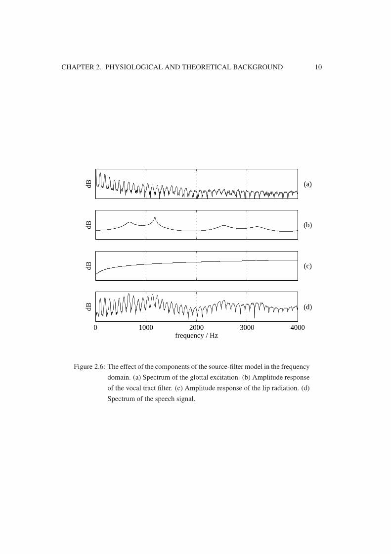
Figure 2.5 illustrates the speech processing mechanism as a series connection of threeseparate and independent processes: glottal excitation, vocal tract filter, and lip radiation.Figure 2.6 shows the effect of these three processes in the frequency domain.
Figure 2.5: Source-filter model.
CHAPTER 2. PHYSIOLOGICAL AND THEORETICAL BACKGROUND 10
dB (a)
dB (b)
dB (c)
0 1000 2000 3000 4000
dB
frequency / Hz
(d)
Figure 2.6: The effect of the components of the source-filter model in the frequencydomain. (a) Spectrum of the glottal excitation. (b) Amplitude responseof the vocal tract filter. (c) Amplitude response of the lip radiation. (d)Spectrum of the speech signal.

Chapter 3
Analysis Methods
Analysis of the vibrating vocal folds during phonation is challenging because the larynxis not easily accessible. However, several techniques have been developed that allow theexamination of the laryngeal activities during voicing.
In general, an analysis technique should reflect the vibratory pattern of the vocal folds orindicate the related acoustic phenomena. It should also be reliable, accurate, and verifiable.Additionally, it is generally desirable that an analysis method be non-invasive, which meansthat no clinical operations are necessary to attach the required measurement equipment inplace, and that the measurement setting interferes with normal speech of the subject as littleas possible. Examination methods of the glottal source differ with respect to these desiredcharacteristics—each method has its advantages and weaknesses.
This chapter describes the voice source analysis techniques that were used in this study.Some background is provided about the history of these methods. Other related techniquesare described briefly as well. Finally, parameters for quantifying the shape of pulses relatedto the glottal activity are introduced.
3.1 Inverse Filtering
The source-filter theory of speech production provides theoretical background for the in-verse filtering technique. If the transfer function of the vocal tract filter is known, an inversefilter can be constructed. In principle, the glottal excitation signal can then be reconstructedby feeding the speech signal through the inverse of the vocal tract filter.
In practice, the transfer function of the vocal tract filter can be approximated based on thespeech signal and general knowledge about the voice production mechanism. An approxi-mate inverse filter can then be constructed. Applying the inverse filter to the speech signalyields an estimate of the excitation signal, the glottal volume velocity waveform. This signal
11

CHAPTER 3. ANALYSIS METHODS 12
is also known as the flow glottogram (FGG) (Hertegård et al., 1992; Hertegård & Gauffin,1995).
Inverse filtering was first presented by Miller (1959), who applied analog electronic filtersto cancel two lowest formants and the lip radiation effect from a speech signal captured bya microphone.
Rothenberg (1973) introduced a different inverse filtering technique that uses the air flowat the mouth as the source signal. The subject’s mouth and nose are surrounded by a specialmask for measuring the flow waveform. This method allows the estimation of absoluteflow values including the DC component, as opposed to the inverse filtering of the pressuresignal captured by a microphone, which loses the absolute zero level of flow due to thelip radiation effect. Rothenberg’s technique is also less sensitive to low-frequency noise.However, the flow measurement mask causes an upper bound on the useful frequency rangeat approximately 1.6 kHz (Hertegard & Gauffin, 1992).
Successful inverse filtering is sensitive to phase distortion in the speech signal in thefrequency range of interest. Traditional tape recorders are problematic for signal storagein this sense since they cause substantial phase distortion, which must be compensatedfor (Childers et al., 1983). This problem has been overcome by tape recorders utilizingfrequency modulation (FM), which fulfills the requirement of phase linearity (Miller, 1959).
Digital filtering techniques provide obvious advantages over analog techniques. Accord-ing to Hunt et al. (1978), a digital inverse filtering approach was applied to speech alreadyby Holmes (1962). Since the 1970’s, inverse filtering has been increasingly realized usingdigital techniques (Hunt et al., 1978; Javkin et al., 1987). Nowadays, practically all inversefiltering methods in use are digital due to the flexibility, repeatability, and ease of imple-mentation of the digital techniques compared to analog filters. Digital sampling and storagetechniques also do not have the phase distortion problem, provided that the equipment is ofhigh quality and the frequency range of flat amplitude response and linear phase responseextends to low frequencies.
Digital inverse filtering methods can be categorized to manual and automatic techniques.Manual methods require the human operator to manually adjust filters to match the formantsof the speech signal, whereas automatic methods build a vocal tract model and automaticallyfind filter parameters, often by means of LPC analysis (Hertegård et al., 1992). There arealso semiautomatic methods that lie somewhere between these two extremes. For example,the method proposed by Alku (1992) basically finds the vocal tract filters automatically butthe user still controls a few parameters that affect the resulting flow signal. Södersten et al.(1999) compared an automatic and a manual inverse filtering method and reported highagreement between the airflow parameters calculated from the flow signals of these twomethods. However, noticeable differences were also encountered.

CHAPTER 3. ANALYSIS METHODS 13
Inverse filtering basically involves extracting two signals, the volume velocity waveformat the glottis, and the effect of the vocal tract filter, from a single source signal. The tech-nique thus implies strong assumptions about the glottal volume velocity waveform and thetransfer function of the acoustic vocal tract filter. Consequently, the result of inverse fil-tering has to be regarded as an estimate of the glottal flow. The actual volume velocitywaveform at the glottis is not known exactly.
Furthermore, the accuracy of inverse filtering deteriorates if the fundamental frequencyof speech is high because the sparse harmonic structure of the excitation spectrum interfereswith formants, which are local resonances in the spectrum. Nasalized vowels are also notsuitable for inverse filtering because their spectra contain antiformants that are difficult tocompensate for properly (Hertegård et al., 1992).
Despite these limitations of the method, inverse filtering has proved to be a valuabletool both for clinical use and for fundamental research of the voice production mechanism(Fritzell, 1992). It is a non-invasive technique that does not require bulky or expensiveequipment. The restrictions of an application may make inverse filtering the only practicalmeans of examining the voice source of a subject.
Figure 3.1 shows a typical example of a speech pressure signal and the correspondinginverse filtered glottal flow waveform.
Pres
sure
Flow
10 ms
Figure 3.1: Speech pressure waveform of a female speaker’s sustained /a/ voweland the corresponding inverse filtered glottal flow waveform.
3.2 Videostroboscopy and Videokymography
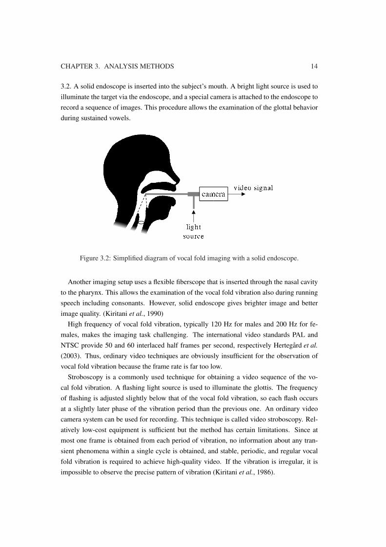
Image recording of the larynx provides valuable information about the physiological move-ments of laryngeal structures during phonation. The experimental setting is shown in Figure
CHAPTER 3. ANALYSIS METHODS 14
3.2. A solid endoscope is inserted into the subject’s mouth. A bright light source is used toilluminate the target via the endoscope, and a special camera is attached to the endoscope torecord a sequence of images. This procedure allows the examination of the glottal behaviorduring sustained vowels.
Figure 3.2: Simplified diagram of vocal fold imaging with a solid endoscope.
Another imaging setup uses a flexible fiberscope that is inserted through the nasal cavityto the pharynx. This allows the examination of the vocal fold vibration also during runningspeech including consonants. However, solid endoscope gives brighter image and betterimage quality. (Kiritani et al., 1990)
High frequency of vocal fold vibration, typically 120 Hz for males and 200 Hz for fe-males, makes the imaging task challenging. The international video standards PAL andNTSC provide 50 and 60 interlaced half frames per second, respectively Hertegård et al.(2003). Thus, ordinary video techniques are obviously insufficient for the observation ofvocal fold vibration because the frame rate is far too low.
Stroboscopy is a commonly used technique for obtaining a video sequence of the vo-cal fold vibration. A flashing light source is used to illuminate the glottis. The frequencyof flashing is adjusted slightly below that of the vocal fold vibration, so each flash occursat a slightly later phase of the vibration period than the previous one. An ordinary videocamera system can be used for recording. This technique is called video stroboscopy. Rel-atively low-cost equipment is sufficient but the method has certain limitations. Since atmost one frame is obtained from each period of vibration, no information about any tran-sient phenomena within a single cycle is obtained, and stable, periodic, and regular vocalfold vibration is required to achieve high-quality video. If the vibration is irregular, it isimpossible to observe the precise pattern of vibration (Kiritani et al., 1986).

CHAPTER 3. ANALYSIS METHODS 15
Videokymography provides means to obtain visual information of the vocal fold vibra-tion at much higher temporal resolution than videostroboscopy. Instead of covering theview of image with several hundreds of scan lines, the brightness along only a single scanline is recorded repeatedly. Scanning frequencies of almost 8000 Hz can be attained usingrelatively inexpensive systems based on ordinary video technology (Švec & Schutte, 1996).The resulting data sequence represents the behavior of the glottal source at one section ofthe vocal folds. It provides relatively high time resolution but does not give informationabout the vibration along the entire length of the vocal folds. An example of a kymogramis shown in Figure 3.3.
Figure 3.3: Kymogram displaying the vibration of the vocal folds along a singleline. The vertical dimension represents time increasing from left toright.
3.3 High-Speed Imaging
Precise visual observation of the vocal fold vibration pattern requires an imaging systemcapable of full images and sufficiently high frame rate. Such systems were initially realizedusing high-speed cinematography. Pictures were exposed on a light-sensitive film usinga high-speed shutter camera. According to various authors (e.g. Švec & Schutte (1996);Eysholdt et al. (1996); Wittenberg et al. (2001)), the method was first developed at the BellTelephone Laboratories in the 1930’s and described by Farnsworth (1940).
This approach had its limitations: large-scale equipment was required, real-time obser-vation of the obtained material was not possible due to the required film processing proce-dure, and frame-by-frame measurements of the vocal fold movements were time-consuming(Kiritani et al., 1986). Furthermore, mechanical noise generated by the system made simul-taneous recording of speech sound impossible (Eysholdt et al., 1996) or at least requiredspecial sound shielding (Kiritani et al., 1986).

CHAPTER 3. ANALYSIS METHODS 16
Digital high-speed camera systems were introduced in the 1980’s (Kiritani et al., 1986,1990). They provide significant benefits over traditional filming techniques: The physicalsize of the required equipment is modest, simultaneous sound recording is possible sincepractically no noise is generated by the equipment, the imagery is instantly accessible, andcomputer-based analysis of the image data is possible.
Temporal and spatial resolution has been a limiting factor with digital devices. In general,there is a trade-off between image resolution and frame rate due to limited data transferspeed. Another limitation on shortening the recording duration of a single image frame isthe illumination of the target. The light has to be fed to the larynx through an endoscopewith a limited diameter, and the power of the light source cannot be increased endlesslybecause this might cause the equipment to heat too much and cause burns in the subject’soral cavities. (Wittenberg et al., 2001)
Image resolutions of 100–300 pixels in each direction and frame rates of approximately2 kHz are common in systems in use. The amount of memory in the high-speed devicealso commonly limits the duration of continuous recording to a few seconds. Most high-speed systems are capable of only gray-scale imaging. Color cameras are also available butusing several color channels implies higher data rates and also increased requirement on theamount of light. (Wittenberg et al., 2001)
Modern digital high-speed cameras reach frame rates of up to 10,000 frames per secondat reasonable resolutions (Weinberger Vision, 2004).
Figures 2.2 and 2.4 show examples of digital high-speed images recorded at a frame rateof 1900 frames per second and a resolution of 256x64 pixels using a Weinberger Speedcamhigh-speed camera and an endoscope that was inserted to the mouth of the subject.
3.3.1 Detection of Vocal Fold Edges and Glottal Area
A widely used method to quantify the image information about the vibrating vocal folds is todetect the edges of the vocal folds and to calculate the area of glottal opening. The sequenceof detected glottal areas of successive image frames is called the glottal area function.The vocal fold edges and thus the glottal area can be detected using manual computer-aided methods (Childers et al., 1983), but automatic computer-based algorithms are alsoavailable, see e.g. Krishnamurthy & Childers (1981); Eysholdt et al. (1996); Larsson et al.(2000).
Usually the material obtained by laryngeal high-speed imaging does not provide absolutedistance measures. However, additional equipment can be used to obtain depth informationin the image, e.g. by using laser triangulation (Hertegård et al., 2003) or stereo imaging(Wittenberg et al., 2000). Depth information also makes it possible to determine absolutedistances from the image.

CHAPTER 3. ANALYSIS METHODS 17
3.4 Electroglottography
Electroglottography (EGG) is a non-invasive method for the examination of the vocal foldvibration. According to several authors (e.g. Colton & Conture (1990); Baken (1992);Henrich et al. (2004)), the method was first reported by Fabre (Fabre, 1940, 1957). Now ithas been used for clinical and research purposes for decades.
Electroglottography is based on measuring impedance across the neck of the speaker.When the vocal folds are closed, electric current can pass through them. When the folds areapart, an insulating air gap separates them, and the impedance across the larynx is higher.Thus, the impedance changes across the larynx indicate the variation of the contact areabetween the focal folds.
Electrodes are placed on the subject’s skin on each side of the larynx and a high-fre-quency alternating current is fed through them in order to measure the impedance betweenthe electrodes. The frequency is typically in the megahertz region and the current is lim-ited to a few milliamperes to ensure that the electric current is imperceptible and harmlessto the subject (Baken, 1992). The voltage between the electrodes is typically about 0.5volts (Marasek, 1997). Figure 3.4 shows the measurement setting with the electrodes on asubject’s skin.
The resulting electroglottographic signal, the electroglottogram, shows the impedancevariation as a function of time. Impedance variation due to vibrating vocal folds is rela-tively small, typically only 1–2 percent of the total measured impedance (Baken, 1992).Furthermore, the impedance varies considerably due to changing skin moistness and ver-tical movements of the larynx. Therefore, high-pass filtering is applied to the obtainedelectroglottographic signal in order to eliminate low-frequency noise and to extract onlythe variations caused by vocal fold vibration. Additionally, automatic gain control is oftenbuilt into EGG devices to maintain appropriate signal level despite considerable impedancechanges between subjects and also during a single recording session. These techniquescause phase and amplitude distortion that may influence the EGG waveform (Scherer et al.,1988, page 291). Consequently, the EGG signal cannot be considered an absolute measureof vocal fold contact, and care must be taken when interpreting the signal.
Despite its limitations, EGG yields useful information about the behavior of the vocalfolds during phonation. Electroglottography has been studied widely and its validity hasbeen assessed by numerous studies comparing EGG with stroboscopic methods, high-speedimaging, photoglottography, subglottal pressure measurements, and inverse filtering, seeHenrich et al. (2004) for references. The results show convincingly that the EGG signal isrelated to the contact area between the vocal folds.
Figure 3.5 shows a typical example of a high-quality electroglottogram recorded during

CHAPTER 3. ANALYSIS METHODS 18
Figure 3.4: EGG measurement setting. Electrodes have been placed on the sub-ject’s skin and a band has been adjusted around the neck to hold theelectrodes in place. The electroglottograph (Glottal Enterprises MC2-1) is on the right on top of the oscilloscope. (Photograph by Anne-Maria Laukkanen)
phonation. It has been high-pass filtered to eliminate the low-frequency components thatare not related to the vibration of the vocal folds.
Rothenberg (1981b) presented a model of the different phases of the EGG signal pe-riod and their relations to the physiological events occurring in the larynx. This model ispresented in Figure 3.6. Other similar models exist, see e.g. Childers et al. (1983). Suchmodels are, however, idealized simplifications that must not be interpreted literally. Manyauthors have pointed out that the EGG signal does not allow exact determination of theinstant of closure, and locating the instant of glottal opening from the EGG signal alone iseven much more inaccurate, see e.g. (Colton & Conture, 1990) and (Baken, 1992).
Titze introduced a mathematical model that describes the vibration pattern of the vocalfolds and predicts the contact area variation, see e.g. Titze (1990). A number of geometric

CHAPTER 3. ANALYSIS METHODS 19
0
EG
GD
iff.
EG
G
Figure 3.5: Electroglottogram of the normal phonation of a male subject. The up-per panel shows the EGG signal and the lower panel its first derivative.Upward change in the signal represents decreasing impedance and thusreduced contact between the vocal folds.
and kinematic parameters are used to describe the shape and movements of the vocal folds,and the model gives the corresponding contact area waveform. The model explains manyfeatures of the contact area waveform by relating them to the physiological pattern of vocalfold vibration: EGG pulse widening is caused by adduction of the vocal folds, and peakskewing is related to wedge-shaped vocal folds and vertical phase difference. A knee inrising and falling edges of an EGG pulse corresponds to the bulging of the contact surfacesof the vocal folds. Vertical phasing also explains the variation of the pulse waveform be-tween a triangular and a rectangular shape. Varying characteristics of real EGG pulses canbe explained as combinations of these effects.
By comparing the EGG waveform with high-speed filming, Childers et al. (1983) relatedthe initial point of vocal fold contact to a break in the negative slope of the EGG waveform,and the glottal opening to the instant at which the differentiated EGG (DEGG) waveformhas its absolute maximum. Such peaks of DEGG are clearly visible in Figure 3.5. Thisapproach was carried on by Henrich et al. (2004), who regarded the peaks of the DEGGsignal as reliable indicators of glottal opening and closing instants defined by reference tothe glottal air flow. However, often such peaks are imprecise or absent, or double peaksoccur. All these cases make this approach unusable.
In addition to resistance across the neck, the impedance measurement is also influencedby reactance (capacitance or inductance) of the examined load. Varying capacitance maybe hypothesized to exist in the glottis when the two vocal folds are separated by a thin insu-lating layer of air, as pointed out by Rothenberg (1981b). This hypothesis can be checked

CHAPTER 3. ANALYSIS METHODS 20
Figure 3.6: The phases of the EGG signal period and their relations to the glottalair flow and physiological events. The figure illustrates the Rothenbergmodel (Rothenberg, 1981b). 1–2: Vocal folds are maximally closed.2–3: Vocal folds are separating from lower margins towards upper mar-gins. 3–4: Upper margins are opening. 4–5: Upper margins are stillopening. Changed slope is due to phase differences along the length ofthe vocal folds. 5–6: Vocal folds are fully parted. The distance betweenthe vocal folds is varying but there is little change in contact area. 6–7:Lower margins are closing with a phase difference along the length ofthe vocal folds. 7–1: Vocal folds are closing from lower margins to-wards upper margins. The flow pulse begins closely after point 3 andterminates closely before point 7.
by changing the frequency of the alternating current used for impedance measurement:the current remains unchanged only if the load is purely resistive. According to Gauffin(Scherer et al., 1988, page 291), the impedance is essentially resistive in a wide frequencyrange.
3.5 Other Analysis Methods
Other analysis techniques are also used. For example, photoglottography (PGG) is a methodthat measures the degree of glottal opening by illuminating the glottis from above or belowand monitoring the light intensity on the other side in order to get an estimate of the glottalarea (Baer et al., 1983).
Titze et al. (2000) described a relatively new technique for examining the glottal source,the electromagnetic glottography (EMGG). It utilizes high-frequency electromagnetic

CHAPTER 3. ANALYSIS METHODS 21
waves to measure tissue motions and does not require skin contact. EMGG may be a viablealternative to traditional electroglottography.
Subglottal pressure is another quantity that is sometimes measured or estimated to exam-ine the laryngeal function. For example, Lecluse et al. (1975) included subglottal pressuremeasurements in their study of EGG devices and the behavior of vocal folds using excisedhuman larynxes, and Hertegård et al. (1995) measured subglottal pressure of a subject dur-ing phonation by means of tracheal puncture.
3.6 Studies Combining Several Analysis Methods
The analysis methods described above are commonly used for validating or evaluating theresults of each other. For example, Henrich et al. (2004) provided a list of comparativestudies that analyze the EGG signal using videostroboscopy, high-speed imaging, inversefiltering, and other methods. Some interesting studies utilizing several analysis techniquesare mentioned below but the list is by no means complete.
Rothenberg (1981b) recorded simultaneously electroglottogram and oral airflow, whichwas then inverse filtered to get an estimate of glottal flow. A seven-stage model of the EGGwaveform with physiological interpretations (see Figure 3.6) was presented as a result.
Baer et al. (1983) compared information obtained by simultaneous and synchronizedhigh-speed filming, acoustic recording, photoglottography, and electroglottography. Theresults indicated high agreement between photoglottography and film measurements withrespect to peak glottal opening and glottal closure, and EGG appeared to indicate vocal foldcontact reliably.
Childers et al. (1983, 1984) recorded synchronously electroglottogram, speech signal,and high-speed film. Glottal flow was obtained by inverse filtering the speech signal. Glottalarea as well as vocal fold contact area were measured from the film. The material was usedto evaluate the validity of electroglottography as an analysis method and to relate the phasesof the EGG waveform to laryngeal events.
Kiritani et al. (1986) compared digital high-speed image sequences with simultaneouslyacquired synchronized speech pressure and EGG signals.
Hertegård et al. (1992) and Hertegård & Gauffin (1995) analyzed simultaneously ob-tained videostroboscopy, inverse filtered flow waveform, and electroglottogram. They pro-vided a schematic illustration of the correspondence between the phases of the glottal vi-bration cycle as seen in the inverse filtered flow waveform and in the laryngeal image.
Schutte & Miller (2001) registered simultaneously electroglottogram, microphone sig-nal, and videokymography. They reported substantial agreement between the informationachieved by EGG and videokymography and showed how videokymography could help

CHAPTER 3. ANALYSIS METHODS 22
avoiding misinterpretations of the EGG signal.Granqvist et al. (2003) examined the relationship between vocal fold vibration and the
glottal flow by comparing simultaneous, synchronized recordings of oral pressure and airflow, sound pressure, inverse filtered glottal flow, EGG, and glottal area function extractedfrom digital high-speed image sequences.
Henrich et al. (2004) evaluated the validity of the differentiated EGG signal as an indi-cation of glottal opening and closure by comparing a simultaneously obtained EGG andhigh-speed recording.
Studies combining inverse filtering, digital high-speed imaging, and electroglottographyare rare. A search for publications of such studies was performed using search enginesaccessing several databases of scientific articles in February 2005. Relevant publicationswere found from only two research groups: Granqvist et al. (2003) utilized all these analy-sis methods synchronously but did not analyze the EGG signal in detail. Sakakibara et al.(2001, 2004) studied throat singing by means of inverse filtering, electroglottography, anddigital high-speed imaging.
3.7 Parametrization of Glottal Flow and Area
closure opening maximum closure
T
To
Tc
Figure 3.7: Schematic diagram of flow pulse phases. The waveform is generated bythe polynomial pulse shape model proposed by Rosenberg (1971). Thelength of the glottal cycle is denoted by T , the length of the openingphase by To, and the length of the closing phase by Tc.
The glottal cycle can be divided to a few phases that are illustrated on the glottal flowpulse in Figure 3.7. Related terminology is introduced below.
Closed phase is the part of the glottal cycle when the vocal folds are in contact along theirentire length and the area of glottal opening is thus zero. There is no air flow betweenthe vocal folds during the closed phase.

CHAPTER 3. ANALYSIS METHODS 23
Opening phase is the phase during which the vocal folds are at least partly separated andthe area of opening between them is increasing. The duration of the opening phase isdenoted by To in Figure 3.7.
Closing phase is the phase during which the vocal folds are separated and the area ofopening between them is decreasing. The duration of the closing phase is indicatedby Tc in Figure 3.7.
Open phase is the part of the glottal cycle during which the vocal folds are separated andair flows through the glottis. Using the symbols of Figure 3.7, the duration of theopen phase is To + Tc.
Closure refers to the instant when the vocal folds come into contact along their entirelength, or when the area of opening between them reaches zero.
Period length, or the length of the glottal cycle, is the time between the correspondinginstants of two successive cycles. This is denoted by T and is the reciprocal of thefundamental frequency f0.
These time measures are used as the basis for time-domain parameters that describe thepulse shape. The parameters used in this work are open quotient, closing quotient, andspeed quotient (Holmberg et al., 1988).
Open quotient (OQ) is defined as the ratio of the open phase length to the total length ofthe glottal cycle.
OQ =To + TcT
(3.1)
A related measure is the closed quotient (CQ), which is the ratio of the closed phaselength to the glottal cycle length. Thus, CQ = 1− OQ. In this work, OQ is used exclusivelyinstead of CQ.
Closing quotient (ClQ) is the ratio of the closing phase duration to the glottal cycle length.
ClQ =TcT
(3.2)
Speed quotient (SQ) is defined as the ratio of the opening phase length to the closingphase length.
SQ =ToTc
(3.3)
Figure 3.8 illustrates how these parameters reflect typical changes in the glottal flowwaveform. The same parameters can be calculated also from other glottal signals than theair flow waveform, e.g. the area of opening between the vocal folds. The resulting param-eter values may not necessarily reflect exactly the same properties of the glottal behavior

CHAPTER 3. ANALYSIS METHODS 24
because, for example, the maximum of air flow does not necessarily occur simultaneouslywith the maximum glottal area.
Parameter Small Large
OQ
ClQ
SQ
Figure 3.8: Synthetic glottal flow pulses that illustrate how the parameters reflect changesin the pulse waveform. Pulses have been generated using the polynomial glottalpulse model introduced by Rosenberg (1971).
Other parameters exist for describing the shape of a glottal pulse waveform. For example,the Normalized Amplitude Quotient (NAQ) (Alku et al., 2002) can be used to parametrizethe closing phase of the flow pulse.
A completely different approach to the parametrization of the flow pulse is to use a para-metric model for describing the glottal volume velocity waveform. A mathematical modelis fit to the observed waveform by finding the most suitable values for the model parameters.These parameters contain information about the most relevant properties of the pulse shape,and they can also be used to reconstruct an approximation of the original pulse waveform.Synthetic glottal pulses can be used for e.g. speech synthesis.
The most commonly used model of glottal volume velocity waveform is the LF model(Fant et al., 1985). It has four parameters that, together with the length of the glottal cycle,uniquely determine the pulse shape. To reconstruct the pulse waveform, a couple of con-struction parameters have to be solved from these specification parameters. This requires anumerical, iterative procedure that is computationally heavy. The computational complex-ity limits the usefulness of the LF model for practical applications (Veldhuis, 1998).
In general, parameters describing the glottal flow waveform can be used for a variety ofpurposes including fundamental research on speech production, clinical use, speech analy-sis, coding, and synthesis, automatic speech recognition, and automatic speaker verificationand identification (Strik, 1998). An example of the utilization of time-based pulse shape pa-rameters is the research reported by Lauri et al. (1997) and Vilkman et al. (1997), in which

CHAPTER 3. ANALYSIS METHODS 25
the effects of vocal loading were studied by means of inverse filtering and the glottal flowpulse parameters OQ, ClQ and SQ. Glottal flow parameters can also be used for quantifyingthe role of the glottal flow waveform in communicating emotion (Gobl & Chasaide, 2003;Airas & Alku, 2004).

Chapter 4
Material and Methods
This chapter describes the material that was studied in this research as well as methodsand techniques for processing the data. The material originates from two separate experi-ments that are referred to as the Huddinge experiment and the HUT experiment. They aredescribed in detail in this chapter. But first, the inverse filtering method IAIF is introduced.
4.1 Matlab Signal Processing and Programming Environment
All digital signal processing, programming, and data visualization was done using the Mat-lab software (The MathWorks, 2004). Matlab versions 6.5, 7.0, and 7.1 were used. TheMatsig signal processing class library for Matlab (Airas, 2004) was also utilized. Customscripts, functions, and user interfaces were developed for the purposes of the work.
4.2 Iterative Adaptive Inverse Filtering (IAIF)
Iterative Adaptive Inverse Filtering (IAIF) is a semi-automatic inverse filtering method de-veloped by Paavo Alku (Alku, 1992; Alku et al., 1999). The method takes a speech pressuresignal as input and generates an estimate of the corresponding glottal flow signal. Blockdiagram of the IAIF procedure is shown in Figure 4.1.
The IAIF algorithm has been improved from that described by Alku (1992) by replacingthe conventional linear predictive coding (LPC) technique with the discrete all-pole (DAP)modeling method (El-Jaroudi & Makhoul, 1991). DAP gives more accurate estimates ofvocal tract formants than the conventional LPC method (Bäckström et al., 2002).
The method operates in two repetitions, hence the word iterative in the name of themethod. These two phases are indicated by gray outlines in Figure 4.1. The first phasegenerates an estimate of the glottal excitation, which is subsequently used as input of the
26

CHAPTER 4. MATERIAL AND METHODS 27
Figure 4.1: Block diagram of the steps of the IAIF method. (Diagram by MattiAiras, MSc(Tech))
second phase to achieve a more accurate estimate. The steps of the method are described indetail below.
1. The input signal is first high-pass filtered to remove disturbing low-frequency fluctu-ations. The high-pass filtered signal is used as the input of subsequent stages. Thecut-off frequency can be adjusted. It should be lower than the fundamental frequencyof the speech signal in order to avoid filtering out relevant information.
2. A first-order DAP analysis is calculated. This step gives an initial estimate of thecombined effect of the glottal flow and the lip radiation effect on the speech spectrum.
3. The input signal is inverse filtered using the filter obtained in step 2. This step effec-tively removes the spectral tilt caused by the spectrum of the excitation signal and thelip radiation effect.
4. The output of the previous step is analyzed by DAP to obtain a model of the vocaltract transfer function. The order p of the DAP analysis is related to the number offormants to be modeled in the analysis frequency band, and it can be adjusted by theoperator of the IAIF method. As a rule of thumb, p should be an even integer that isobtained by adding a small number to the sampling frequency of the analyzed signalin kHz (Markel & Gray, 1976).
5. The input signal is inverse filtered using the inverse of the pth-order model from step4.

CHAPTER 4. MATERIAL AND METHODS 28
6. The output of the previous step is integrated in order to cancel the lip radiation effect.This yields the first estimate of the glottal flow and completes the first repetition.
7. The second repetition starts by calculating a gth-order analysis of the obtained glottalflow estimate. This gives a spectral model of the effect of glottal excitation on thespeech spectrum. The value of g is usually between 2 and 4.
8. The input signal is inverse filtered using the model of the excitation signal to eliminatethe glottal contribution.
9. Lip radiation is canceled by integrating the output of the previous step.
10. A new model of the vocal tract filter is formed by an rth order DAP analysis. Thevalue of r can be adjusted by the user but it is commonly set equal to the value of pin step 4.
11. The effect of the vocal tract is removed from the input signal by inverse filtering itwith the vocal tract model obtained in the previous step.
12. Finally, the lip radiation effect is canceled by integrating the signal. This yields thefinal estimate of the glottal flow, which is the output of the IAIF method.
The conversion from volume velocity at the mouth to the radiating pressure signal is com-monly modeled by a simple differentiation operation, which in the digital signal processingdomain is represented by the following transfer function:
L(z) = 1− z−1 (4.1)
When the source for inverse filtering is the pressure signal, this lip radiation effect hasto be canceled by the inverse filtering procedure in order to obtain the glottal flow wave-form. The inverse of L(z) above amounts to integration. However, this cannot be directlyused in practice since integration implies infinite gain at zero frequency and great amplifi-cation at low frequencies. This would lead to instability and undesired behavior in practicalimplementation. (Javkin et al., 1987)
Consequently, inverting the effect of lip radiation is typically realized by the followingleaky integrator
IL(z) =1
1− ρz−1(4.2)
where ρ is an adjustable parameter whose value is slightly below unity.The integration blocks of the IAIF method are realized using the leaky integrator. The
constant ρ can be varied within a small range below 1. The closer the value is to unity,the more exactly the leaky integration corresponds to the inverse effect of differentiation.

CHAPTER 4. MATERIAL AND METHODS 29
Decreasing ρ makes the integrator more leaky, which decreases low-frequency amplifica-tion and makes the output signal value approach the zero level faster. The parameter ρ iscontrolled by the user of the IAIF method to make the flow waveform most plausible byadjusting the waveform approximately horizontal in the closed phase.
IAIF applies the same filtering procedure to the entire signal to be processed, so the inputsignal is assumed to exhibit a stable vocal tract configuration. The method can be usedto inverse filter a lengthy segment of speech in so far as this assumption holds. However,typically the inverse filtered signal is no longer than a couple of hundreds of millisecondsto ensure minimal changes in the vocal tract transfer function. The signal should not be tooshort either: a minimum of a few periods is recommended to get reliable results.
4.2.1 HUT IAIF Toolbox
HUT IAIF Toolbox is a Matlab implementation of IAIF developed mainly by Matti Airasat the Laboratory of Acoustics and Audio Signal Processing at Helsinki University of Tech-nology. The inverse filtering procedure is controlled through the graphical interface shownin Figure 4.2.
First, a WAV audio file is chosen and a portion of it is selected for inverse filtering. Then,IAIF parameters are tuned to get a plausible glottal flow signal as a results. Controls forsetting the most relevant parameters are located in the IAIF parameters box of the userinterface. The Max # of formants slider adjusts the order of the DAP models: p and rare set to twice the chosen number of formants. g is 4 by default. Another settings windowallows setting p and r individually and also changing g, but typically this possibility is notused.Lip radiation is the ρ parameter used in the integrating stages of IAIF. The cut-off
frequency of the high-pass prefiltering stage is controlled by the Highpass slider but thecut-off can also be chosen to be automatically set to a slightly lower frequency than thefundamental frequency in the selected speech segment. The toolbox determines the funda-mental frequency automatically by calling the Matsig implementation of the YIN algorithm(de Cheveigné & Kawahara, 2002).
The input signal as well as the resulting flow estimate are shown in the signal window,see Figure 4.3. The upper panel shows the high-pass filtered speech signal and indicatesthe portion of it selected for inverse filtering. The lower panel displays the resulting flowestimate in blue. The gray signal is obtained by simply integrating the input signal. Thissignal window is updated automatically when the IAIF parameters are modified or the inputsignal selection is changed.
Additional features of HUT IAIF Toolbox include spectral display of signals and DAPmodels, automatic determination of inverse filtering parameters, and automatic NAQ pa-

CHAPTER 4. MATERIAL AND METHODS 30
Figure 4.2: The graphical user interface of HUT IAIF Toolbox, which is a Matlabimplementation of the IAIF method.
rameter calculation.
4.3 Huddinge Experiment
4.3.1 Recording Setup
The first set of data to be analyzed in this study was collected in an experiment that wascarried out at the Huddinge University Hospital of the Karolinska Institute in Stockholm,Sweden, in April 2004. There were three subjects, one female and two males. They allwere adults with healthy voices and long experience in voice research.
The experiment consisted of two parts. In the first part, the subjects produced sustained/æ/ vowels in three phonation modes: breathy, normal, and pressed. The duration of eachphonation was approximately one second. The phonations were produced in rapid succes-sion so that the entire sequence of three phonations took no longer than four seconds. Eachsubject repeated this at least three times.
In the second part, four sustained /æ/ vowels were produced with loudness increasing

CHAPTER 4. MATERIAL AND METHODS 31
Figure 4.3: The signals window of HUT IAIF Toolbox. The upper panel showsthe high-pass filtered speech pressure signal. The yellow rectangle onbackground indicates the signal segment selected for inverse filtering.In this case, the entire visible signal is selected. The lower panel dis-plays the integrated pressure signal in gray and the inverse filtered flowsignal in blue. The inverse filtering settings are shown in Figure 4.2.
from phonation to phonation. These vowels were slightly less than one second in durationand they were also produced in rapid succession to fit the whole sequence in a four-secondtime window. The subjects repeated this task three times.
The voice production in all these phonations was measured using three techniques simul-taneously. See also Figure 4.4.
1. Speech pressure signal was captured using a Brüel & Kjær condenser microphone4192 and a Brüel & Kjær microphone amplifier 2669. The microphone was placed ata distance of 10 centimeters from the subject’s mouth. The distance was controlledin the beginning of each recording.
2. Electroglottogram was recorded by means of a Glottal Enterprises MC2-1 electro-glottograph. The electrodes were placed on the subject’s neck and conducting paste

CHAPTER 4. MATERIAL AND METHODS 32
was applied between the electrodes and the skin. A flexible band was adjusted aroundthe neck over the electrodes to hold them in place.
3. Digital high-speed image sequence of the vocal folds was obtained via a rigid endo-scope and recorded by a Weinberger Speedcam +500 high-speed camera. A 300 Wxenon lamp (R. Wolf) was used as the light source. The endoscope was inserted intothe subject’s mouth and the operating physician held the subject’s tongue.
The video image sequence was digitized by a frame grabber card on a computer. Asequence of digital grayscale images with 256 gray levels was obtained. The reso-lution was 64x256 pixels and the frame rate approximately 1900 frames per second.The maximum length of continuous video recording was limited by the memory size(128 MB) of the frame grabber device to 8192 frames, or 4.3 seconds.
At the end of each phonation, the high-speed image capturing process was stoppedby pressing a foot pedal. The last 8192 frames before the instant of this pedal presswere then saved on hard disk without any compression.
The image from the high-speed camera was also shown in real time on a computerscreen.
For the synchronization of the microphone and EGG signals with the video image se-quence, an additional synchronization channel was included. Synchronization was arrangedby recording the state of the pedal, which stopped the imaging, on the synchronizationchannel. The beginning of the pedal pulse thus indicated the instant of the last image andprovided the primary means of synchronization.
Due to the lack of synchronization between the video frame rate and the sound card sam-pling rate, the pedal pulse alone would provide sufficient synchronization accuracy only in arelatively short time window at the end of the image sequence. Therefore, an improvementwas made to the synchronization method used in e.g. the study by Granqvist et al. (2003).The video signal from the high-speed camera was summed to the synchronization channelat a low amplitude. No image information could be obtained from this synchronization sig-nal, but the frame synchronization pulses in the video signal caused a strong spectral peakat the frequency of the frame rate. Consequently, this arrangement allowed exact extractionof the frame rate from the synchronization signal.
The three signals—pressure captured by the microphone, EGG, and the synchronizationsignal—were digitized by a multichannel sound card using 16 kHz sample rate and 16 bitsper sample. The data was then stored in a sound file on a computer hard disk. The durationsof these recordings varied between 8 and 40 seconds. The 4.3-second time span of thehigh-speed image sequence was completely covered in all recordings.

CHAPTER 4. MATERIAL AND METHODS 33
Figure 4.4: The Weinberger high-speed camera with the endoscope attached. Themicrophone is attached to the stand and is positioned in front of thesubject’s mouth. EGG electrodes are placed on the subject’s neck be-low a supporting band. (Photograph by Anne-Maria Laukkanen)
Each sequence of three phonations in different phonation modes or four phonations withincreasing loudness was stored separately. One sound file with three channels and oneimage sequence file was created for each such recording. Additional data files were alsoproduced containing information about the camera frame rate, resolution, etc.
Figure 4.5 shows an example of a recorded sound file of breathy, normal, and pressedphonation. The pedal pulse is clearly visible on the synchronization channel, and the rawvideo signal is seen as low-amplitude ripple on this channel.

CHAPTER 4. MATERIAL AND METHODS 34
Figure 4.5: Three-channel recording of breathy, normal, and pressed phonation.The video signal is seen as low-amplitude ripple on the synchronizationchannel. The pedal pulse indicating the instant of the last high-speedimage is clearly visible.
4.3.2 Data Selection and Preprocessing
The quality of the EGG signals turned out to be inconsistent. In many cases, the EGGsignal was too noisy to be used as a reliable source of information about the glottal behavior.Figure 4.6 shows an example of such a noisy EGG signal. Due to the apparently unreliablesignal quality, the EGG recordings of the Huddinge data were not used in this study, exceptfor the analysis of the signal synchronization accuracy as described in Section 4.3.7.
10 ms
Figure 4.6: Example of a noisy EGG signal.

CHAPTER 4. MATERIAL AND METHODS 35
An obvious discontinuity was detected in two of the high-speed image recordings. Thisindicated that something unexpected had happened to the image data. Consequently, thesetwo recordings were discarded altogether. Three to four recordings of each subject remainedfor the analysis of the different phonation modes, and three recordings of each subject wereavailable for the loudness variation cases.
In the loudness variation recordings, the first phonation was found to be too soft in manycases. Therefore, the weakest phonation was omitted and only the last three phonationswere examined in each recording.
A sequence of five consecutive glottal periods was then chosen for examination in eachof the phonations to be analyzed. Primarily, the periods were chosen approximately at themiddle of the phonation. However, this requirement was relaxed if, e.g., the signal was notstationary in the middle part of the phonation or if the high-speed image sequence began ata later time instant for the first phonation in a recording.
An analysis window was then marked around each five-cycle sequence. The windowextended up to a couple of periods to both directions from the sequence of five analysisperiods. The durations of the windows varied between 30 and 80 milliseconds dependingon the fundamental frequency of phonation.
4.3.3 Calculation of the Sound Pressure Level
The sound pressure level (SPL) of each analysis window was estimated from the micro-phone signal recording. A calibration signal for the SPL calculation was recorded at thedata collection session prior to starting the phonation measurements. Any changes in therecording setup, e.g. adjusting the gain setting, were followed by the recording of a newcalibration signal. Annotations were made indicating the calibration signal to be used witheach data recording.
The calibration signals were obtained by placing a calibrator device tightly against themicrophone and recording the microphone output in the same way as phonations wererecorded. A Brüel&Kjær Sound Level Calibrator, Type 4231, was used as the calibrator.It provided a sinusoidal pressure signal whose frequency was 1000 Hz ± 0.1 % and soundpressure level 94.00 dB ± 0.20 dB.
Sound pressure level is defined as
Lp = 20 log10
p
p0(4.3)
= 10 log10
p2
p20
where p is the effective root-mean-square (RMS) sound pressure, and the reference pressureis p0 = 20 µPa. Since the microphone signal is directly proportional to the sound pressure,

CHAPTER 4. MATERIAL AND METHODS 36
the sound pressure level can be expressed in terms of the digitized microphone signal x[n]as follows:
Lp = 10 log10
x2rms
x20
(4.4)
where x0 is the root-mean-square value of the microphone signal corresponding to the ref-erence pressure p0, and xrms is the root-mean-square value of the microphone signal in thetime range of interest:
xrms =
√√√√ 1N
k+N∑
n=k+1
(x[n])2 (4.5)
Since applying this to the calibration signal xc[n] has to yield Lp = 94 dB, the referencevalue x0 can be eliminated and the formula for the SPL is
Lp = 10 log10
1N
∑(x[n])2
1Nc
∑(xc[n])2 + 94 dB. (4.6)
The calibration signals were high-pass filtered using a digital 2048-tap linear-phase FIRfilter to remove low-frequency noise components. The choice of the exact cut-off frequencyhad very little effect on the RMS value of a filtered calibration signal as long as the cut-off was above a few herz and well below the calibration signal frequency 1 kHz. Thiswas verified by a simple experiment in which the cut-off frequency was varied between20 Hz and 700 Hz. Less than 0.05 % variation was found in the RMS values. Basedon this result, a cut-off frequency of 100 Hz was chosen. It seemed safe to assume that thefiltering removed disturbing low-frequency noise sufficiently without affecting considerablythe actual calibration signal.
The calibration signals were then examined visually and auditorily. A stable sequencewas cut from each signal and its root-mean-square value was computed and stored. Thedurations of these calibration sequences varied between 2.5 and 4.5 seconds.
Equation 4.6 was then applied to calculate the sound pressure levels of the analysis win-dows marked in the phonations. No frequency weighting was applied.
The correctness of the SPL calculation procedure was verified by two tests. First, a por-tion of each calibration signal was run through the same steps as the phonation recordings,including the high-pass filtering stage in the HUT IAIF Toolbox software. The obtainedSPL values were within 0.01 dB from 94 dB. Second, the signal values of one calibrationsignal were divided by two and the same test was repeated. The SPL dropped by 6 dB asexpected.

CHAPTER 4. MATERIAL AND METHODS 37
4.3.4 Inverse Filtering
Each analysis window was inverse filtered using the HUT IAIF Toolbox, which was de-scribed in Section 4.2.1. The cutoff frequency of the high-pass filter was set a few percentbelow the fundamental frequency of each phonation. The parameters of the IAIF methodwere adjusted manually as follows. The goal was to obtain a plausible flow waveform withapproximately constant value in the closed phase if possible. The number of formants,which controls the IAIF parameters p and r described in Section 4.2, was set to the lowestvalue that gave a reasonable result. It was varied between 6 and 11. The lip radiation coeffi-cient, indicated by ρ in Equation 4.2, was then adjusted to give an approximately horizontalclosed phase. The range of values was from 0.972 to 0.997.
Other parameters of the HUT IAIF Toolbox were not altered from their default values.Thus, p and r were always equal and g was 4. See section 4.2 for a detailed description ofIAIF and its parameters.
Parametrization of Flow Pulses
The flow waveforms obtained by inverse filtering were parametrized using open quotient(OQ), closing quotient (ClQ), and speed quotient (SQ), which were introduced in Section3.7. The instants of closure, opening, and maximum flow were marked manually in the flowpulses.
It turned out that the flow often showed pulse waveforms similar to the one shown inFigure 4.7. The instant of closure is followed by a relatively short closed phase with nearlyconstant flow. Then, the flow starts to increase gently. This phase ends abruptly at a kneethat begins a segment with more rapid flow increase. Thus, there are two instants that couldbe considered instants of glottal opening. From now on, these instants are referred to asthe primary opening, which is the end of the horizontal phase, and the secondary opening,which is the instant of abrupt increase of flow derivative.
To study this phenomenon and its relation to the glottal behavior visible in the imagesequence, the two opening instants were marked in flow pulses in which this phenomenonappeared. Two open quotients (OQ1 and OQ2) and speed quotients (SQ1 and SQ2) werethen calculated correspondingly:
OQ1 =To1 + Tc
T(4.7)
OQ2 =To2 + Tc
T(4.8)
SQ1 =To1Tc
(4.9)

CHAPTER 4. MATERIAL AND METHODS 38
T
Tc
To2
To1
Figure 4.7: Flow pulse with primary and secondary opening. The length of theglottal cycle is denoted by T . The interval from the primary opening tothe instant of maximum flow is indicated by To1 and the interval fromthe secondary opening to the instant of maximum flow by To2. Theclosing phase length is denoted by Tc.
SQ2 =To2Tc
(4.10)
If a flow pulse did not show two opening instants, the two opening marks were positionedat the same instant. In this case, OQ1 = OQ2 and SQ1 = SQ2.
4.3.5 Glottal Area Function
Automatic Detection of Glottal Area
The glottal area waveform in each high-speed video sequence was extracted automaticallyusing the custom-made software High-speed Toolbox, version 2.0. The software has beendeveloped by Hans Larsson. (Larsson et al., 2000)
The user interface of the software consists of several windows. The main window, shownin Figure 4.8 (a), is used for adjusting the video display and for controlling the analysisprocedure. The video image is displayed in a separate window as shown in Figure 4.8 (b).
The detection of glottal area is performed in the following steps:
1. The desired high-speed video file is opened, the file position slider is moved to theportion of interest, and the area calculation mode is activated.
2. The software detects automatically the range of interest within the image area basedon brightness variations in a sequence of successive frames. This area can be dis-

CHAPTER 4. MATERIAL AND METHODS 39
(a) (b)
Figure 4.8: The High-Speed Toolbox software (Larsson et al., 2000). (a) The mainwindow with user controls. (b) The related video frame display. Thedetected edge of glottal opening is also displayed on top of the videoimage.
played in the video window, and its borders can be manually dragged to desiredlocations.
3. Now, the software tries to detect the edges of the glottis in the active frame. It firsthigh-pass filters the selected range of interest in horizontal direction. Edge trackingis then performed based on maximal derivative in the image, an adjustable gray level,and the detected edge in the previously analyzed frame (Larsson et al., 2000). Thedetected edges of the glottis can be displayed on top of the video image, as shown inFigure 4.8 (b). The gray level utilized by the algorithm is adjusted using the Marklev slider in the main window in order to obtain correct edge positions. Movingin the video sequence is possible, so the results of edge detection can be checked indifferent phases of the vibration cycle.
4. After setting the area of interest and the gray level optimally, the area calculation isstarted. It takes a couple of minutes to process the entire sequence of eight thousandframes on a machine with AMD Athlon(tm) XP 2400+ processor.

CHAPTER 4. MATERIAL AND METHODS 40
5. The detected edges can now be examined for each frame, and the obtained area func-tion can be shown in a separate window. The edges can also be adjusted manually foreach frame individually using the mouse.
6. Finally, the resulting area function is saved to file.
The area detection procedure does not give an absolute area measure since the dimensionsof the glottis in the image are generally not known. The software supports absolute areameasurement by using a laser triangulation technique (Hertegård et al., 2003). However,this capability was not utilized in this study because no laser triangulation equipment wasused in the data recording setting.
Additionally, the High-Speed Toolbox software is capable of generating a kymogramover a selected portion of the file at a specified scan line in the image, but this feature wasnot used in this study.
Limitations of the Area Function
Care must be taken when interpreting the glottal area waveforms acquired by the High-Speed Toolbox software. Several issues limit the reliability of the obtained area function:
• The actual borders of the vocal folds are not easy to distinguish in the figure even bya human observer. The task is complicated by suboptimal illumination conditions,relatively low spatial resolution of the video image, and physiological phenomena.The mucosal wave, or the vertical phase difference of the vocal fold vibration, makesthe vocal fold edge often hard to follow accurately, especially because the lowermargin is often not well illuminated. Also, the opening phase is often gradual: Themiddle of the glottis starts to get darker but it is not easy to determine the instant whena gap actually opens between the vocal folds. Finally, a minor chink is frequentlyobserved, especially in the case of the female subject, in either the posterior or theanterior part of the glottis or in both parts. See Figure 4.9 for an example. However,there is no clear-cut boundary between cases where a chink exists and where the vocalfolds close completely.
• The automatic area detection is highly sensitive to the gray level adjustment madeby the operator of the software. Finding an optimal level setting often involves acompromise: If the gray level is set too low, dark areas surrounding the glottis areoften erroneously detected as part of the glottal opening in some of the frames. Ifthe level is set too high, the ability of the software to detect a narrow glottal openingdeteriorates.

CHAPTER 4. MATERIAL AND METHODS 41
Figure 4.9: Anterior and posterior chink in the most closed phase of the glottalcycle in female subject’s normal phonation.
• High-Speed Toolbox is relatively poor at detecting the edges of the vocal folds whenthe opening is narrow. Often, the instant of glottal opening would be placed manuallyat the previous frame compared to what the automatic algorithm yields. The sameapplies to the instant of closure, so the manual examination would commonly giveopen phases that are a couple of frames longer. Unfortunately, High-Speed Toolboxdoes not seem to allow setting the glottal area easily by hand for frames in which noopening has been found.
• Especially in pressed phonations, the vocal folds are often partially hidden by otherstructures above the glottis. An example is shown in Figure 4.10. In such cases, itis impossible to measure the actual area of opening between the vocal folds fromthe image data. The visible opening can be measured with some accuracy, but thismeasure does not necessarily correspond to the actual glottal opening that determinesthe air flow to the vocal tract.
Figure 4.10: Two examples of the glottis being partially hidden by supraglottalstructures in pressed phonation.
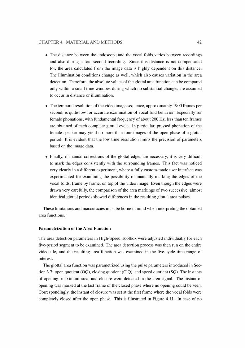
CHAPTER 4. MATERIAL AND METHODS 42
• The distance between the endoscope and the vocal folds varies between recordingsand also during a four-second recording. Since this distance is not compensatedfor, the area calculated from the image data is highly dependent on this distance.The illumination conditions change as well, which also causes variation in the areadetection. Therefore, the absolute values of the glottal area function can be comparedonly within a small time window, during which no substantial changes are assumedto occur in distance or illumination.
• The temporal resolution of the video image sequence, approximately 1900 frames persecond, is quite low for accurate examination of vocal fold behavior. Especially forfemale phonations, with fundamental frequency of about 200 Hz, less than ten framesare obtained of each complete glottal cycle. In particular, pressed phonation of thefemale speaker may yield no more than four images of the open phase of a glottalperiod. It is evident that the low time resolution limits the precision of parametersbased on the image data.
• Finally, if manual corrections of the glottal edges are necessary, it is very difficultto mark the edges consistently with the surrounding frames. This fact was noticedvery clearly in a different experiment, where a fully custom-made user interface wasexperimented for examining the possibility of manually marking the edges of thevocal folds, frame by frame, on top of the video image. Even though the edges weredrawn very carefully, the comparison of the area markings of two successive, almostidentical glottal periods showed differences in the resulting glottal area pulses.
These limitations and inaccuracies must be borne in mind when interpreting the obtainedarea functions.
Parametrization of the Area Function
The area detection parameters in High-Speed Toolbox were adjusted individually for eachfive-period segment to be examined. The area detection process was then run on the entirevideo file, and the resulting area function was examined in the five-cycle time range ofinterest.
The glottal area function was parametrized using the pulse parameters introduced in Sec-tion 3.7: open quotient (OQ), closing quotient (ClQ), and speed quotient (SQ). The instantsof opening, maximum area, and closure were detected in the area signal. The instant ofopening was marked at the last frame of the closed phase where no opening could be seen.Correspondingly, the instant of closure was set at the first frame where the vocal folds werecompletely closed after the open phase. This is illustrated in Figure 4.11. In case of no

CHAPTER 4. MATERIAL AND METHODS 43
complete closure, the instants of opening and closure were set at the frame with minimumarea of opening.
T
To T
c
Figure 4.11: Phases of a glottal area pulse. The figure shows glottal cycle length T ,opening time To, and closing time Tc derived from the area waveform.
All instants of opening, maximum area, and closure were checked manually by visualinspection of the image sequence. If necessary, the marks based on the automatically ac-quired area function were corrected. Indeed, changes were made in this manual checkingstage. The most frequent reason was the inability of High-Speed Toolbox to detect a narrowslit between the vocal folds. Therefore, the opening marks were often moved backward andthe closure marks forward by one frame.
Consequently, the automatically obtained area function was not directly used for parame-trization or analysis of the glottal behavior. The area function provided, however, an impor-tant visualization that improved the understanding of the glottal behavior and also served asa basis for the manual corrections.
4.3.6 Error Estimates of Individual Pulse Parameters
Due to the limited frame rate of the high-speed imaging system, samples of the glottal areacan be obtained relatively sparsely. If the closing, opening, and maximum instants of thearea function are assumed to be located correctly, each such instant is marked to the frameclosest to the true instant of the event. The maximum error of each measured time instantis thus one half of the time between two successive video frames.
This limits the precision of the pulse parameters OQ, ClQ, and SQ that are derived fromthe image material. It is important to assess the precision of these parameters to avoidmaking conclusions of minor variations that may actually be caused by measurement un-certainty.

CHAPTER 4. MATERIAL AND METHODS 44
The same source of uncertainty applies to the microphone and EGG signals, but the errorsare much smaller because the sample rate (16 kHz) is almost ten times higher than the framerate of the high-speed image sequence (1900 Hz).
Error Propagation
Suppose that a parameter y is calculated from measured quantities x1, x2, . . ., xn.
y = f(x1, x2, . . . , xn) (4.11)
Also suppose that absolute limits ∆xi of measurement errors are available. The truevalue of each measured quantity is thus known to be in the range xi ±∆xi. These errorswill cause an error ∆y in the calculated parameter y.
A general method for getting the formula of propagating error is based on the conceptof total differential (Vaari, 1994). If each variable xi changes by a small amount dxi, theeffect on y is given by the total differential
dy =(∂f
∂x1
)dx1 +
(∂f
∂x2
)dx2 + . . .+
(∂f
∂xn
)dxn. (4.12)
The error in y caused by measurement errors is obtained by replacing the differentials dxiby the corresponding error limits ∆xi. To get an upper bound for ∆y, all error estimatesas well as partial derivatives are assumed to be positive. This method gives the followingformula for the error estimate of y:
∆y =∣∣∣∣∂f
∂x1
∣∣∣∣∆x1 +∣∣∣∣∂f
∂x2
∣∣∣∣∆x2 + . . .+∣∣∣∣∂f
∂xn
∣∣∣∣∆xn (4.13)
If the error terms ∆xi are not considered absolute limits of error but statistical bounds,probable errors, or uncertainties, a different formula has to be used. According to Doebelin(1975), it can be shown (Scarborough, 1955) that a proper method for combining sucherrors is using the root-sum square formula:
Erss =
√(∂f
∂x1∆x1
)2
+(∂f
∂x2∆x2
)2
+ . . .+(∂f
∂xn∆xn
)2
(4.14)
This yields an error Erss that has the same meaning as the individual errors ∆xi. Theresulting error estimate is always smaller than that given by Equation 4.13 (Doebelin, 1975).In this work, however, this approach was not used.
Error Limits of Pulse Parameters
Figure 4.12 shows an idealized glottal pulse. The instants required for calculating pulseparameters from the waveform are indicated in the figure.

CHAPTER 4. MATERIAL AND METHODS 45
Figure 4.12: Idealized glottal pulse waveform. The instants required for calculat-ing time-based pulse parameters are indicated: closure (tc0 and tc1),opening (to1), and maximum (tm1).
Let us denote the time intervals estimated from the pulse as follows:
• Cycle length T = tc1 − tc0
• Opening time To = tm1 − to1
• Closing time Tc = tc1 − tm1
The instant of each event in the signal is assumed to be marked correctly to the sampleclosest to the actual event. Thus, the absolute limit of each time error can be assumed to behalf the time between two successive samples. This is denoted by ∆t.
∆to1 = ∆tc0 = ∆tc1 = ∆t =1
2fs(4.15)
An estimate of the fundamental frequency is obtained as the reciprocal of the cycle lengthestimate:
f0 =1T
=1
tc1 − tc0 . (4.16)
An upper bound on the absolute error of f0 can be obtained using the total differentialmethod.
∆f0 =
∣∣∣∣∣∂f0
∂tc0
∣∣∣∣∣∆tc0 +
∣∣∣∣∣∂f0
∂tc1
∣∣∣∣∣∆tc1 (4.17)
Solving the partial differentials yields
∆f0 =∣∣∣∣
1(tc1 − tc0)2
∣∣∣∣∆tc0 +∣∣∣∣
−1(tc1 − tc0)2
∣∣∣∣∆tc1. (4.18)
Using the notation introduced above, this can be rewritten as
∆f0 =1T 2
∆t+1T 2
∆t
=2T 2
∆t. (4.19)

CHAPTER 4. MATERIAL AND METHODS 46
This is a practical formula for the maximum error in the fundamental frequency estimatecaused by the limited sampling frequency.
Open quotient (OQ) is defined as the ratio of the open phase length to the cycle length.The open quotient estimate acquired from the pulse in Figure 4.12 is thus
OQ =tc1 − to1tc1 − tc0 . (4.20)
The total differential method gives the following upper bound on the absolute error propa-gated to the OQ estimate.
∆OQ =
∣∣∣∣∣∂OQ∂to1
∣∣∣∣∣∆to1 +
∣∣∣∣∣∂OQ∂tc0
∣∣∣∣∣∆tc0 +
∣∣∣∣∣∂OQ∂tc1
∣∣∣∣∣∆tc1 (4.21)
Solving the partial differentials yields
∆OQ =∣∣∣∣−1
tc1 − tc0
∣∣∣∣∆to1 +∣∣∣∣tc1 − to1
(tc1 − tc0)2
∣∣∣∣∆tc0 +∣∣∣∣to1 − tc0
(tc1 − tc0)2
∣∣∣∣∆tc1 (4.22)
which can be rewritten as
∆OQ =1T
∆t+To + Tc
T 2∆t+
T − To − TcT 2
∆t
=2T
∆t. (4.23)
Similarly, closing quotient (ClQ) is defined as the ratio of the closing phase length to thecycle length and is estimated from the time instants shown in Figure 4.12 by the formula
ClQ =tc1 − tm1
tc1 − tc0 . (4.24)
The total differential method yields the following estimate of the upper bound on the abso-lute error of ClQ.
∆ClQ =
∣∣∣∣∣∂ClQ∂tm1
∣∣∣∣∣∆tm1 +
∣∣∣∣∣∂ClQ∂tc0
∣∣∣∣∣∆tc0 +
∣∣∣∣∣∂ClQ∂tc1
∣∣∣∣∣∆tc1
=∣∣∣∣−1
tc1 − tc0
∣∣∣∣∆tm1 +∣∣∣∣tc1 − tm1
(tc1 − tc0)2
∣∣∣∣∆tc0 +∣∣∣∣tm1 − tc0
(tc1 − tc0)2
∣∣∣∣∆tc1
=1T
∆t+Tc
T 2∆t+
T − TcT 2
∆t
=2T
∆t (4.25)
Finally, the speed quotient (SQ) estimate is
SQ =tm1 − to1tc1 − tm1
. (4.26)

CHAPTER 4. MATERIAL AND METHODS 47
and its error limit is obtained as follows.
∆SQ =
∣∣∣∣∣∂SQ∂to1
∣∣∣∣∣∆to1 +
∣∣∣∣∣∂SQ∂tm1
∣∣∣∣∣∆tm1 +
∣∣∣∣∣∂SQ∂tc1
∣∣∣∣∣∆tc1
=∣∣∣∣−1
tc1 − tm1
∣∣∣∣∆to1 +∣∣∣∣tc1 − to1
(tc1 − tm1)2
∣∣∣∣∆tm1 +∣∣∣∣−(tm1 − to1)(tc1 − tm1)2
∣∣∣∣∆tc1
=1Tc
∆t+To + Tc
T 2c
∆t+To
Tc2 ∆t
= 2To + Tc
Tc2 ∆t
= 2To+TcT
Tc2
T 2T
∆t
= 2OQ
ClQ2T
∆t (4.27)
Error Limits of Averaged Pulse Parameters
Representative parameter values are commonly estimated by averaging the parameters cal-culated from a few successive glottal cycles:
y =1N
N∑
n=1
yn (4.28)
Absolute error limits of the mean can be obtained from the error limits of individual param-eter values yn using the total differential method. Since
∂y
∂yn=
1N, (4.29)
Equation 4.13 implies that the error bound of the mean is the mean of the individual errorbounds.
Applying this principle to the mean pulse parameters of successive glottal cycles givesthe upper bound on the error of the mean caused by low temporal resolution. The approachassumes that the time instants are perfectly assigned to the respective signal samples andthat all examined pulses are identical.
The glottal pulse parameters extracted from successive glottal periods are not completelyindependent. The closure instant is used as the end mark of one cycle and the beginningmark of the next cycle. Therefore, error in the timing of a closure instant affects both thepreceding and the following cycle. This interdependency is ignored in this error analysis.
Another commonly used method for estimating the error limits of the mean of measuredvalues is to calculate the standard error of the mean (SEM), which is derived from the

CHAPTER 4. MATERIAL AND METHODS 48
variance of individual measured values. It is calculated using the following formula (Vaari,1994; Klaucke et al., 2004; Pindyck & Rubinfeld, 1998):
SEM =
√∑(yi − y)2
N(N − 1)(4.30)
It can be stated with 95 percent confidence that the mean of the measured characteristic isbetween y − 1.96 SEM and y + 1.96 SEM (Pindyck & Rubinfeld, 1998).
According to Klaucke et al. (2004), the standard error of the mean can be used as anestimate of confidence if the characteristic to be measured is normally distributed, or if thedistribution is not normal but the sample size is greater than 30. In this study, only fiveconsecutive glottal cycles were averaged, and it is probably not safe to assume that thepulse parameters are normally distributed. Moreover, due to the relatively low frame rateof the imaging system, it is not uncommon that a pulse parameter estimation yields exactlythe same value from five successive cycles of the glottal area waveform. In such cases, theSEM equals zero and fails to give any useful information about the real uncertainty of theparameter value. However, also in these cases, the error limits derived from the temporalresolution using the total differential method give an appropriate estimate of the uncertaintycaused by the limited time resolution.
Consequently, two complementary error estimates were calculated for each average pulseparameter:
1. The uncertainty caused by the limited time resolution is quantified by the mean ofthe error bounds of individual parameter values. This does not take into account anyvariation between successive cycles nor errors in marking the time instants of eventsin the glottal waveforms.
2. The standard error of the mean (SEM) is calculated from the variance of individualparameter values and the 95 % confidence interval is derived from the SEM. Lowtemporal resolution of the glottal area data causes this measure to be useless in somecases, and the low number of samples in the calculation of mean also deteriorates thereliability of the SEM-based uncertainty estimate.
4.3.7 Synchronization
Pedal Pulse
Since the high-speed image sequence was stored separately from the other signals, explicitsynchronization was required. For the comparison of glottal area waveform with the corre-sponding glottal flow signal, it was essential to find exactly which area pulse corresponds

CHAPTER 4. MATERIAL AND METHODS 49
to each flow pulse. Much more accurate synchronization of the flow and area signals wouldbe necessary to assess temporal differences between the waveforms in detail.
The pedal pulse, which stopped the high-speed imaging, was recorded on the synchro-nization channel. The beginning of the pedal pulse was detected automatically from eachrecording by finding the position of maximum derivative of the synchronization signal. Thisindicated the instant of the last video frame.
An obvious source of uncertainty in this method is that the pedal pulse does not occur insynchrony with the video frames and, consequently, the time difference between the pulseand the last frame varies between 0 and 1 frames. Granqvist et al. (2003) examined thesynchronization error between the pedal pulse and the last frame in a similar experimentalsetup. They recorded a periodically varying light signal simultaneously by a light diodeand the high-speed camera. Comparison of these two recordings showed that the time shiftbetween the pedal pulse and the last video frame was 0.27 frames on average with standarddeviation of 0.39 frames.
Based on this result, the instant of the last frame was shifted backward from the beginningof the pedal pulse by 0.27 frames also in this study. Consequently, the timing of the lastframe was set slightly prior to the pedal pulse. However, this procedure does not removethe uncertainty indicated by the standard deviation of the time shift in the measurementsmade by Granqvist et al. (2003).
If the error is assumed to be caused purely by the random timing of the pulse betweentwo successive video frames, the theoretical standard deviation can be calculated easily.The probability density function of the pedal pulse f(x) is supposed to be uniform in thetime range from 0 to 1 frames and zero outside this range. Thus, the expected value of delayis
µ =∫ 1
0xf(x) dx =
12
(4.31)
and the standard deviation
σ =
√∫ 1
0(x− µ)2f(x) dx ≈ 0.29, (4.32)
which is less than the empirically measured value 0.39. Thus, there is more uncertaintyrelated to the timing of the last frame and the pedal pulse than just the interval between twosuccessive frames. In other words, the last frame may actually occur more than one frametime after the pedal pulse.
Video Frame Rate
Granqvist et al. (2003) also stated that the synchronization drifted as the distance from thepedal pulse increased because the sound card sample rate and the frame rate of the high-

CHAPTER 4. MATERIAL AND METHODS 50
speed camera were not synchronized. In this study, this source of timing error was reducedby including the video signal on the synchronization channel. This provided means tomeasure the video frame rate in the postprocessing stage. Figure 4.13 shows a short excerptof the synchronization signal. Despite the relatively low sample rate, the frame rate isevident.
1 ms
Figure 4.13: Video signal on the synchronization channel. The frame rate of ap-proximately 1900 Hz can be obtained accurately from the signal.
The frame rate was estimated from each synchronization signal by the following proce-dure:
1. Hanning window was applied to the synchronization signal of the entire recording.
2. Fast Fourier Transform (FFT) of one million points was computed from the win-dowed signal to get the spectrum.
3. The highest peak of the amplitude spectrum in the frequency range from 1880 Hz to1910 Hz was located. This was used as the estimate of frame rate.
Synchronization signals were examined by listening. This revealed that in many casesthe the microphone signal was audible also on the synchronization channel at a level al-most comparable to the video synchronization signal. The video synchronization tone atapproximately 2 kHz varied in intensity and timbre between recordings and also withineach recording. However, it was almost impossible to assess perceptually if there was alsovariation in the fundamental frequency of the synchronization signal.
The stability of the frame rate was examined by applying the frame rate estimation pro-cedure to different parts of each recording: the entire file, the duration of the stored videosequence (4.3 s), the first half of the stored video sequence (2.1 s), and the last half of thestored video sequence (2.1 s). The results showed that differences between the frame rateestimates of different portions of a recording differed by less than 0.1 Hz in most cases. In

CHAPTER 4. MATERIAL AND METHODS 51
all but two cases, the maximum difference was less than 0.3 Hz. For two recordings, themaximum difference was almost one frame per second, but also in these cases the differ-ence between the frame rate estimate of the entire file and the portion of the stored videorecording was less than 0.3 Hz.
The frame rates estimated from the entire recordings were between 1891.7 Hz and 1892.3Hz except for one recording whose frame rate was 1904.8 Hz. This deviant recording alsohad a break in the image sequence and was discarded. Another file showed an interestingphenomenon: very close to the moment of the pedal press, the frame rate jumped approxi-mately from 1892 Hz to 1898 Hz. Since this happened at the end of the image sequence, itwas considered harmless. Similar behavior was not found in any other recording.
As a result, the frame rate estimated from each entire recording was considered reliableenough to be used for the synchronization of high-speed images with the other signals. Thiswas supposed to give more accurate synchronization than using the frame rate saved to adata file during the recording since this was given at the precision of one Hz only. Indeed,visual inspection showed no considerable synchronization drift between the area and flowwaveforms during the 4.3-second time span of each image sequence. The uncertainty of theexact position of the pedal pulse relative to the last frame was considered larger than thatcaused by the inaccuracy of the frame rate estimate.
The video signal on the synchronization channel also opened up the possibility of moreexact timing of the last video frame by means of the video signal phase. However, it wasnot known at which point of the video frame cycle the image was actually obtained from thephoto sensors and whether this happened instantaneously for the entire image. Furthermore,there was no way or eliminating the uncertainty of whether one more frame occurs after thepedal pulse or not. Therefore, the video signal phase was not used for correcting the timingof the last frame relative to the pedal pulse.
Propagation Delay
Electroglottography and high-speed imaging indicate movements of laryngeal tissues prac-tically instantly, whereas a significant delay is associated with the propagation of the acous-tic signal from the vocal folds to the microphone. Therefore, to examine the laryngealevents originating in the larynx at the same instant of time, the microphone signal has tobe shifted relative to the other signals. The propagation delay is determined by the distancefrom the sound source to the microphone and the speed of sound in the medium.
The length of the vocal tract is typically approximately 17 centimeters for men and 15centimeters for women. During the recording, the distance from the subject’s mouth to themicrophone was tried to keep constant at 10 centimeters. Thus, the distance from the glottisto the microphone was 27 centimeters and 25 centimeters for male and female subjects,
CHAPTER 4. MATERIAL AND METHODS 52
respectively. The speed of sound was approximated to be 350 m/s, which is probably arelatively accurate approximation in the conditions where the air is warmed by the humanbody temperature.
Thus, the microphone signal was shifted for males by
∆t =0.27
350 ms
= 0.771 ms. (4.33)
Similarly for females, it was shifted by
∆t =0.25
350 ms
= 0.714 ms. (4.34)
This corresponds to 11–12 samples at the sample rate of 16 kHz.
Evaluation of Synchronization Accuracy
The accuracy of synchronization between the obtained signals was assessed by comparingthe waveforms. Especially, the instant of glottal closure was detected in the signals becauseit can be detected most reliably. It corresponds to the instant of major excitation of the vocaltract system within a pitch period because the glottis closes abruptly and opens more slowly(Strube, 1974).
Several algorithms have been proposed for locating the glottal closure instant (GCI) inthe acoustic signal automatically. One such method detects discontinuities of the differen-tiated speech signal (Ananthapadmanabha & Yegnanarayana, 1975). Many other methodsare primarily based on the linear prediction error, which is large at the location of glottalclosure (Strube, 1974; Ma et al., 1994). Several improvements to this basic principle havebeen developed utilizing e.g. maximum-likelihood epoch determination and Hilbert trans-form (Cheng & O’Shaughnessy, 1989), Frobenius norm approach (Ma et al., 1994), or thegroup delay function (Smits & Yegnanarayana, 1995). Since the detection of glottal closurewas used only for the evaluation of synchronization in this study, the instant of major exci-tation was estimated manually based on the instant of an abrupt change in the microphonesignal.
The instant of glottal closure occurs in the glottal flow signal at the position where theflow drops abruptly to the base level. This is illustrated in Figure 3.7.
In the electroglottographic signal, the glottal closure causes a steep, abrupt decrease inthe waveform, as shown in Figure 3.6. According to Henrich et al. (2004), the peak in thederivative of the EGG signal can be regarded as a reliable indication of the instant of glottalclosure in the modal register.
The glottal area signal, of course, drops to zero at the point of glottal closure.

CHAPTER 4. MATERIAL AND METHODS 53
These definitions of the glottal closure instant are based on different signals and may thusbe related to slightly different physiological events during the closing phase. However, timedifferences between those instants should not be large.
The maximum acoustic excitation located in the microphone signal seemed to coincidewith the glottal closure as detected from the inverse filtered flow signal. The peak of theDEGG waveform also matched well with the end of the glottal area pulse in general. How-ever, the closure was consistently marked at an earlier instant of time in the microphone andflow signals as compared to the EGG or area signals. In several cases, the timing differencewas as much as 0.5 milliseconds, which corresponds to more than 15 cm in distance, andthe pressure signal never seemed to lag the EGG signal. Furthermore, the distance from thesynchronization pulse was not found to have any consistent effect on the magnitude of thesynchronization offset.
An example of the evaluation of synchronization accuracy is shown in Figure 4.14. Theclosure instant of the flow waveform coincides with the location of excitation in the pressuresignal. Also, the DEGG peak occurs between the time instants of the last non-zero areasample and the following zero-valued area sample.
The observed synchronization shift has approximately the same magnitude as the uncer-tainty related to the alignment of the high-speed image sequence with the other signals. Theinstants of closure detected in the different signals are also related to different physiolog-ical phenomena and they may thus not occur exactly simultaneously, which causes someuncertainty in the evaluation of synchronization accuracy.
Due to the uncertainty of synchronization, accurate temporal within-period comparisonsbetween the area function and the inverse filtered flow waveform were not considered rea-sonable. However, the synchronization error was small compared to the cycle length, andthe area pulse corresponding to each flow pulse could thus be identified exactly. Conse-quently, pulse-by-pulse comparisons of signal waveforms were possible.

CHAPTER 4. MATERIAL AND METHODS 54
0
5 ms
Pres
sure
Dif
f. p
ress
.Fl
owE
GG
DE
GG
Are
a
Figure 4.14: Evaluation of signal synchronization. The figure shows the followingsignals from top to bottom: pressure captured by microphone, dif-ferentiated pressure, inverse filtered glottal flow, EGG, differentiatedEGG, and glottal area extracted from the high-speed image sequence.Propagation delay has been compensated for by shifting the pressuresignal and the flow signal. Two instants of closure, indicated by grayvertical lines, have been located manually in the flow waveform andin the EGG signal. The acoustic signal shows an abrupt change atthe closure instant found in the flow signal, whereas the closure inthe area function matches well with the instant of closure detectedin the electroglottogram. The mismatch between the two instants isapproximately 0.4 milliseconds, which is similar in magnitude to theuncertainty of the alignment of the high-speed image sequence. Theinstants detected in different signals are related to different physiolog-ical phenomena, which causes some uncertainty in this comparison.

CHAPTER 4. MATERIAL AND METHODS 55
4.4 HUT Experiment
4.4.1 Recording Setup
The second experiment was conducted in the anechoic chamber of the Laboratory of Acous-tics and Audio Signal Processing at Helsinki University of Technology in May 2003. Therewere 13 subjects, 6 females and 7 males. Most of them were young adults and none hadvoice disorders.
The subjects were asked to phonate sustained /a/ vowels five times in sequence, first inbreathy, then in normal, and finally in pressed phonation. The duration of each phonationwas approximately one second.
Phonations were captured by a Brüel & Kjær 4188 condenser microphone that was at-tached to a Brüel & Kjær Mediator 2238, which is a sound pressure level meter and alsofunctions as a microphone amplifier. The signal was recorded on a DAT tape. The distancefrom the subject’s mouth to the microphone was 40 cm, and special attention was paid tokeeping it constant. The distance was controlled and, if necessary, corrected during therecording session.
Electroglottogram was recorded simultaneously with the acoustic signal. A Glottal En-terprises MC2-1 electroglottograph was used. Another channel of the DAT tape was usedfor storing the EGG signal.
The signals were stored on the digitally on the tape using 48 kHz sample rate and 16 bitsper sample. The data were later moved to a computer hard disk.
The same material is used in another study that compares the flow waveforms obtainedby several operators of two different inverse filtering methods (Lehto et al., 2005).
4.4.2 Data Selection and Preprocessing
The sampling rate was reduced to 22.05 kHz using the downsampling feature of the CoolEdit Pro software version 1.2a.
A segment of ten successive glottal periods was selected for analysis from every subject’sbreathy, normal, and pressed phonation. Primarily, the segment was chosen from the thirdof the five phonations of the same phonation type, starting at 100 milliseconds after thebeginning of the phonation. However, this rule was not followed strictly in some caseswhere a more stable and more representative sample was obtained at another position orwhere the subject had made more than five phonations.

CHAPTER 4. MATERIAL AND METHODS 56
4.4.3 Calculation of the Sound Pressure Level
Sound pressure level was measured from each window of interest in the same way as de-scribed in Section 4.3.3. The Brüel&Kjær Sound Level Calibrator of type 4231 was usedalso in this experiment. A calibration file was recorded in the beginning of the recordingsession. Gain settings were not altered during the experiment, so this calibration file appliesto all recordings.
4.4.4 Inverse Filtering
The selected segments of the phonations were inverse filtered using the HUT IAIF Toolboxsoftware, which was introduced in Section 4.2.1.
First, the cutoff frequency of high-pass filtering was set automatically eight percent belowthe fundamental frequency of the phonation. The number of formants was then set to thelowest value that gave a reasonable glottal flow waveform. The value of this parametervaried between 7 and 15 for these signals. Finally, the lip radiation term was adjusted in therange from 0.97 to 0.9975 so that a horizontal closed phase appeared in the flow waveformif possible. Other parameters had default values.
The high-pass filtering phase reduced the length of the analyzed signal segment from 10periods by a couple of periods because part of the signal was required to fill the filter’sinternal memory, which is necessary for the filtering operation to stabilize.
4.4.5 Electroglottogram
The EGG signals obtained in this experiment were superior in quality to those obtainedfrom the Huddinge experiment. The sample electroglottogram in Figure 3.5 was acquiredfrom a normal phonation of a male subject in this experiment. It is a good example of avery clean EGG signal as compared to the one in Figure 4.6.
The EGG signals were high-pass filtered digitally using a 2048th-order linear-phase FIRfilter with cutoff frequency at 70 Hz. This removed low-frequency fluctuations that wereconsiderably large in the EGG signal.
4.4.6 Compensation of the Propagation Delay
The sound propagation from the glottis to the microphone was compensated in order toassess the glottal behavior at the same instant of time in both the inverse filtered flow wave-form and the EGG. Therefore, the EGG signal was delayed relative to the sound pressuresignal and the inverse filtered flow signal.
The vocal tract length was assumed to be 15 cm for female subjects and 17 cm for male

CHAPTER 4. MATERIAL AND METHODS 57
subjects. The distance from the subject’s mouth to the microphone was 40 cm in the record-ing setting, so the total travel distance was 55 cm and 57 cm for women and men, respec-tively. The speed of sound was supposed to be 350 m/s. The delay was thus approximately1.6 ms, or 35–36 samples at the sampling rate of 22.05 kHz.
After compensating for the sound propagation delay, the synchronization of the micro-phone and EGG signals was assessed by comparing the instants of closure detected manu-ally from the microphone signals, inverse filtered flow waveforms, and differentiated EGGsignals. Good agreement was found in these comparisons. Based on this observation andthe fact that the microphone distance was repeatedly controlled in the recording session,the synchronization was considered accurate enough for temporal comparisons of instantsdetected in the inverse filtered flow waveforms and the corresponding EGG waveforms.
4.4.7 Parametrization of Glottal Flow and EGG
Detailed behavior of the inverse filtered flow pulses and the EGG waveforms in the openingand closing phases were of major interest for this data set. Also, it was assumed that thecompensation of the sound propagation delay was quite accurate. Therefore, instead ofthe quotients introduced in Section 3.7, exact instants of significant events in the flow andEGG waveforms were detected. Automatic algorithms were developed and tuned for thispurpose.
Glottal Flow Waveform
Locating instants of significant events in the flow waveform was based on three signals:
1. The inverse filtered flow itself.
2. The first derivative of the flow. This was constructed by simply calculating the dif-ference of consecutive sample values.
3. A smoothed second derivative of the flow signal. Basically, this signal was producedby first applying a Gaussian mask to the signal to smooth it and then differentiatingthe result twice. Since these operations are linear, the same result can be obtained bydifferentiating the Gaussian mask twice and then applying it to the original signal.This procedure yields the mask shown in Figure 4.15. A similar mask shape can beobtained as a difference of two Gaussians with different standard deviations. This isknown as the Difference of Gaussians (DoG) operator, or the Mexican Hat operator.It is used in edge detection applications. (Owens, 1997)
The Gaussian mask was computed by
y = e−( t0.05T )2
(4.35)

CHAPTER 4. MATERIAL AND METHODS 58
Figure 4.15: Mask for calculating the smoothed second derivative. The shape isobtained by differentiating a Gaussian mask twice.
Flow
0
1st d
eriv
.
0
Smoo
thed
2nd
deri
v.
Figure 4.16: Significant instants detected from the glottal flow waveform. Inversefiltered flow is shown in the top panel, first derivative of the flowin the middle panel, and smoothed second derivative in the bottompanel. The detected instants are marked as follows: ©maximum flow,H negative peak of the flow derivative, O closure, M primary opening,and N secondary opening. Gray lines illustrate the regression linesthat have been fit to the opening phase of the flow waveform.
where T is the length of the glottal cycle.
Figure 4.16 shows an example of these three signals calculated from a single flow pulse.The following instants were detected from each flow period:
1. The instant of maximum flow was detected as the maximum of the inverse filteredflow signal within the cycle.
2. The instant of primary excitation was located as the minimum of the flow derivativebetween two successive flow maxima.

CHAPTER 4. MATERIAL AND METHODS 59
3. The range of flow variation during the cycle was defined as the range from the lowestflow level between two successive flow maxima to the flow level at the precedingmaximum. A threshold was set at 15 % above the bottom of this flow range. Theinstant of closure was then determined by searching forward from the instant of neg-ative peak of the flow derivative until a point was found where the flow was belowthe threshold and the flow derivative had a positive value.
4. For the detection of the primary opening instant, another flow range and thresholdwere defined. The minimum of the range was set at the average flow value during the10 % of the period length after the instant of closure, and the maximum was the flowlevel at the next flow maximum. A threshold was defined at 10 % above the bottomof this range. The instant of primary opening was then found in two stages: First, theflow signal was scanned backward from the next flow maximum until the flow valuedropped below the threshold. Then, the backward scanning was continued as longas either the flow derivative was positive or the preceding 5 % of the glottal periodcontained a flow value lower than 1 % of the flow range below the flow value at thecurrent scanning position. The instant of primary opening was then set at the pointwhere this search algorithm stopped. However, the opening instant was not allowedto occur before the instant of closure.
5. Finally, the instant of secondary opening was located at the largest local maximum ofthe smoothed second derivative of the flow signal in the time window starting 5 % ofthe period after the primary opening and extending up to the next flow maximum.
Furthermore, the sharpness of the knee in the flow waveform at the secondary openingwas assessed quantitatively. Two regression lines were fit to the flow signal using the least-squares criterion, one between the primary opening and the secondary opening, and theother between the secondary opening and the following flow maximum. Such regressionlines are shown in gray in Figure 4.16. The slopes of these two lines are denoted here by k1
and k2, respectively. The sharpness of the knee was quantified by
S =k1 − k2
flowmax − flowminT (4.36)
where flowmax is the value of the flow at its maximum, flowmin is the minimum flowvalue within the period, and T is the length of the glottal period.
Electroglottogram
Similarly, the instants corresponding to the glottal opening and closure were identified au-tomatically in each cycle of the electroglottogram. The detection was based on the first

CHAPTER 4. MATERIAL AND METHODS 60
derivative of the EGG signal (DEGG). Figure 4.17 illustrates the EGG waveform and itsderivative during one glottal cycle and also indicates the detected instants of closure andopening.
EG
G
0
DE
GG
Figure 4.17: Glottal closure and opening detected from the EGG waveform: clo-sure and × opening. The top panel shows the EGG waveform and thebottom panel its first derivative, the differentiated EGG.
1. The instant of glottal closure was determined in the time window between two suc-cessive flow maxima as the first local minimum of the DEGG signal that was lessthan 25 % above the global minimum in this time window.
2. The instant of glottal opening was located as the maximum of the DEGG signal inthe time window between the EGG closure instant and the next flow maximum.
The sharpness of the opening peak was also assessed by a quantitative measure. Themaximum value of the DEGG signal was searched in a time window of 40 % ofthe glottal cycle length around the opening peak, excluding the 10 % of the glottalcycle in the middle of that window. This value, denoted by DEGGwin, was thus themaximum of the DEGG in the neighborhood of the peak excluding the very closestvicinity. The dashed vertical lines in Figure 3.6 indicate the borders of this window.The sharpness of the opening peak was then quantified by the measure
P =DEGGmax −DEGGwinEGGmax −EGGmin T (4.37)
where DEGGmax is the maximum value of the opening peak in DEGG, EGGminandEGGmax are the minimum and maximum values of the EGG signal between twosuccessive flow maxima, and T is the cycle length. The purpose of the denominator inthe formula is to normalize the measure to variations in the EGG amplitude, whereasT normalizes variations in the fundamental frequency.
Chapter 5
Results
This chapter reports the results obtained using the material and methods described in theprevious chapter. Numerical data and graphical illustrations are provided. Special, unex-pected findings are also reported. Further analysis and explanations of the results is thetopic of Chapter 6.
5.1 Huddinge Experiment
The data files of the Huddinge experiment were numbered with consecutive numbers whenthe recordings were saved. Altogether, 20 recordings were successful and were examined.Each of them contained three phonations that were analyzed.
In this thesis, the three subjects are referred to as Female 1, Male 1, and Male 2. Eachrecording is denoted by a combination of subject and recording number, e.g. Male1-06. In-dividual phonations are indicated by the recording identification followed by the phonationtype: breathy, normal, or pressed for phonation modes, and soft, normal, or loud in case ofloudness variation. The loudness referred to as normal does not necessarily correspond tothe subject’s habitual way of speaking but it refers to the second last of the four phonationsin this phonation task. See Sections 4.3.1 and 4.3.2 for details of the recording setting anddata selection.
Table 5.1 lists all the recordings.
5.1.1 Sound Pressure Level Estimates
Sound pressure level estimates were calculated for each analyzed phonation from the signalin the analysis window as described in Section 4.3.3. Recording settings were changedseveral times during the experiment. Therefore, several calibration files were used for SPLcalculation.
61

CHAPTER 5. RESULTS 62
Table 5.1: Huddinge recordings. File numbers between 19 and 37 were used foranother type of experiment which is not included in this work.
Recording Subject File Phonation task
Male1-03 Male 1 finnl03a breathy, normal, pressedMale1-05 Male 1 finnl05a breathy, normal, pressedMale1-06 Male 1 finnl06a breathy, normal, pressedMale1-07 Male 1 finnl07a breathy, normal, pressedMale1-08 Male 1 finnl08a soft, normal, loudMale1-09 Male 1 finnl09a soft, normal, loudMale1-10 Male 1 finnl10a soft, normal, loudMale2-12 Male 2 finnl12a breathy, normal, pressedMale2-13 Male 2 finnl13a breathy, normal, pressedMale2-14 Male 2 finnl14a breathy, normal, pressedMale2-15 Male 2 finnl15a breathy, normal, pressedMale2-16 Male 2 finnl16a soft, normal, loudMale2-17 Male 2 finnl17a soft, normal, loudMale2-18 Male 2 finnl18a soft, normal, loudFemale1-38 Female 1 finnl38a breathy, normal, pressedFemale1-39 Female 1 finnl39a breathy, normal, pressedFemale1-40 Female 1 finnl40a breathy, normal, pressedFemale1-41 Female 1 finnl41a soft, normal, loudFemale1-42 Female 1 finnl42a soft, normal, loudFemale1-43 Female 1 finnl43a soft, normal, loud
Tables 5.2 and 5.3 show the results of SPL calculation. For each recording, the SPLis shown for all three phonations. The difference in SPL between each pair of successivephonations is also presented. Additionally, the table indicates the calibration file that isrelated to each recording according to the annotations made during the recording session.Figures 5.1 and 5.2 illustrates the SPL estimates graphically.
A listening check revealed that the background noise level changes notably betweenrecordings 07 and 08 but not between recordings 08 and 09 where the annotations indi-cate a change of the calibration signal. Similarly, listening indicated a change in noise levelbetween recordings 16 and 17. According to the notes, however, the calibration file was notchanged here. Since assigning calibration files to recordings by listening would involve toomuch guesswork, the results shown here are based on the annotations, but suspicious casesare marked by asterisks in Table 5.3. Fortunately, the SPL values are not salient results ofthis study.
In each recording, the SPL increases consistently from breathy to pressed phonation and

CHAPTER 5. RESULTS 63
Table 5.2: Sound pressure level estimates of vowels in different phonation types inthe Huddinge experiment. Sound pressure levels are given in dB withlinear weighting.
Recording Calibration file Breathy ∆ Normal ∆ Pressed
Male1-03 kalib 81.3 6.6 87.9 1.8 89.7Male1-05 kalib 82.7 4.6 87.3 1.4 88.7Male1-06 kalib 81.9 5.7 87.6 2.1 89.7Male1-07 kalib 80.3 5.6 85.9 2.7 88.6Male2-12 kalib2 71.6 3.1 74.7 4.3 79.0Male2-13 kalib2 73.3 7.7 81.0 3.3 84.3Male2-14 kalib2 70.7 10.5 81.2 3.5 84.7Male2-15 kalib2 77.0 5.5 82.5 6.4 88.9Female1-38 kalib3 77.2 5.0 82.2 15.0 97.2Female1-39 kalib3 72.7 7.6 80.3 9.9 90.2Female1-40 kalib3 75.8 3.5 79.3 2.7 82.0
Table 5.3: Sound pressure level estimates of phonations at different loudness in theHuddinge experiment. Sound pressure levels are given in dB with linearweighting. Three recordings are marked with an asterisk (*) indicatinga probable confusion with the calibration files.
Recording Calibration file Soft ∆ Normal ∆ Loud
Male1-08 kalib* 77.3 10.0 87.3 6.9 94.2Male1-09 kalib2 95.6 5.0 100.6 5.4 106.0Male1-10 kalib2 94.3 6.8 101.1 4.8 105.9Male2-16 kalib2 88.7 12.2 100.9 8.7 109.6Male2-17 kalib2* 74.0 17.4 91.4 10.4 101.8Male2-18 kalib2* 80.1 7.0 87.1 10.0 97.1Female1-41 kalib4 76.4 13.1 89.5 12.2 101.7Female1-42 kalib4 79.6 8.3 87.9 19.5 107.4Female1-43 kalib4 87.0 12.9 99.9 2.8 102.7
from soft to loud phonation as expected. Yet, there are considerable differences in SPLvalues between subjects but also between the phonations of the same subject within thesame phonation type. Some of the within-subject variation may be explained by errors inthe notes about calibration files, but remarkable variation still remains. This indicates thatthe phonations vary in their acoustic features even in consecutive recordings of the samesubject and the same phonation task.

CHAPTER 5. RESULTS 64
60 70 80 90 100 110
male1−03
male1−05
male1−06
male1−07
male2−12
male2−13
male2−14
male2−15
female1−38
female1−39
female1−40
dB
breathynormalpressed
Figure 5.1: Sound pressure level estimates of vowels in different phonation typesin the Huddinge experiment.

CHAPTER 5. RESULTS 65
60 70 80 90 100 110
male1−08
male1−09
male1−10
male2−16
male2−17
male2−18
female1−41
female1−42
female1−43
dB
softnormalloud
Figure 5.2: Sound pressure level estimates of phonations at different loudness inthe Huddinge experiment.

CHAPTER 5. RESULTS 66
5.1.2 Qualitative Observations
Figure 5.3 shows the pressure, flow, and area signals of phonation Male1-06-normal. Thehigh-speed images from three instants are also shown. The flow signal exhibits a clear two-stage opening phase. However, no glottal opening can be seen in the image taken shortlyprior to a secondary opening.
Pres
sure
Flow
Are
a
Figure 5.3: Phonation Male1-06-normal. No glottal opening can be seen in the vo-cal fold image in the middle even though the flow signal has increasedfrom the base level.
Figure 5.4 is a similar illustration of the phonation Male2-12-breathy. The glottis is notcompletely closed in this example. This was typical of the breathy phonations examined inthis study.
A minor opening between the vocal folds was commonly observed in the most closedphase of the glottal cycle in the female subject’s normal phonations. Figure 4.9 shows anexample of a chink at both the anterior and the posterior parts of the vocal folds. Occa-sionally, a probable chink was also seen in normal phonations of the subject Male 2 andin pressed phonations of the female subject. The existence of a minor chink complicated
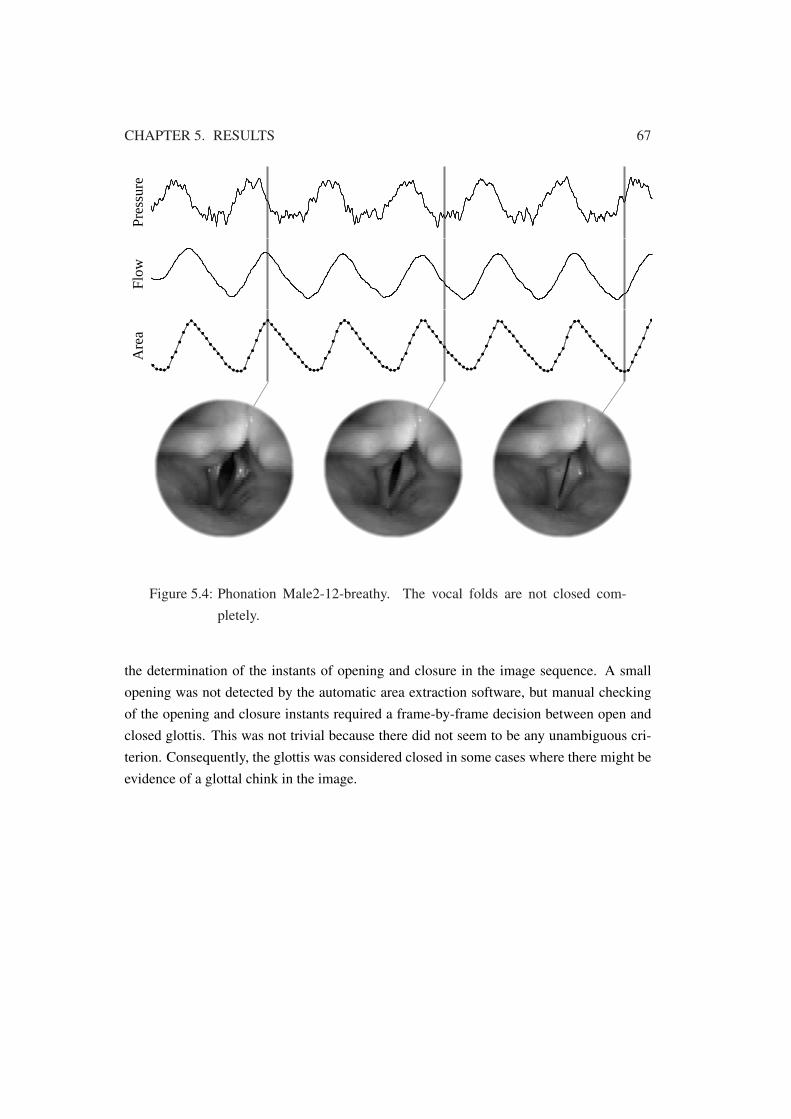
CHAPTER 5. RESULTS 67Pr
essu
reFl
owA
rea
Figure 5.4: Phonation Male2-12-breathy. The vocal folds are not closed com-pletely.
the determination of the instants of opening and closure in the image sequence. A smallopening was not detected by the automatic area extraction software, but manual checkingof the opening and closure instants required a frame-by-frame decision between open andclosed glottis. This was not trivial because there did not seem to be any unambiguous cri-terion. Consequently, the glottis was considered closed in some cases where there might beevidence of a glottal chink in the image.

CHAPTER 5. RESULTS 68
5.1.3 Pulse Parameters
Numerical parameters were calculated from each cycle of glottal flow and area within theanalysis windows. Error bounds were estimated for each parameter as described in Section4.3.6. Figure 5.5 shows the parameters obtained from the phonations of the subject Male 1at normal loudness. Error limits are illustrated by vertical lines with horizontal end markers.An example of the flow pulse waveform and the area pulse waveform in each phonation isalso shown. Appendix A contains similar figures of all examined cases.
140160180
0.4
0.6
0.20.30.4
0.51
1.52
2.5
Male1−08 Male1−08Male1−09 Male1−09Male1−10 Male1−10Flow Area
f 0 / H
zO
QC
lQS
QP
ulse
s
Figure 5.5: Parameters estimated from the phonations of the subject Male 1 at nor-mal loudness. Each column with five values for each parameter cor-responds to one recording from which five successive glottal periodshave been analyzed. For OQ and SQ, cross (×) denotes primary open-ing and dot (•) denotes secondary opening. Vertical lines with horizon-tal end markers indicate estimated error boundaries due to limited timeresolution. For each phonation, the flow waveform and the correspond-ing area pulse of one glottal cycle are also shown at the bottom of thefigure.
Originally, the aim was to calculate a set of representative parameters for each subject inall phonation type and loudness categories by averaging the parameter values of all the ana-lyzed periods of the subject and phonation task in question. However, successive recordingsof the same subject and phonation type turned out to have quite different characteristics in

CHAPTER 5. RESULTS 69
some cases. This is evident in Figure 5.5 where the fundamental frequency, pulse wave-form, and pulse parameters vary considerably from recording to recording. However, theparameter values extracted from successive glottal periods within a single recording aremuch more consistent.
The observed variation of parameters is not surprising. The speaking conditions were farfrom normal in the recording situation because of the endoscope that was inserted into thesubject’s mouth. Furthermore, several minutes elapsed between successive recordings dueto necessary preparations of the equipment.
Consequently, it seemed reasonable to apply averaging only to parameter values origi-nating from quite similar glottal pulses. This was particularly true for parameters differen-tiating between primary and secondary opening: there was no point in averaging e.g. OQ2
values over a collection of phonations that contained cases where a clear secondary openingwas found and cases where it was not found. Therefore, only one representative phonationwas chosen for each combination of speaker and phonation type, and the pulse parameterswere averaged from the five consecutive cycles in this phonation.
The phonations selected for further analysis of parameters are listed in Table 5.4. Theselection was based on the following criteria:
• Typical occurrence of the desired phonation type as assessed by subjective listening.
• High image quality and good visibility of the glottis.
• EGG signal quality.
Table 5.4: Phonations selected for parameter analysis.
Phonation Male 1 Male 2 Female 1
Breathy Male1-06-breathy Male2-12-breathy Female1-40-breathyNormal Male1-06-normal Male2-14-normal Female1-39-normalPressed Male1-06-pressed Male2-14-pressed Female1-39-pressedLoudness 1 Male1-09-soft Male2-16-soft Female1-42-softLoudness 2 Male1-10-normal Male2-17-normal Female1-42-normalLoudness 3 Male1-09-loud Male2-16-loud Female1-41-loud
5.1.4 Mean Pulse Parameters
Phonation Modes
Average parameters of the selected phonations in different phonation modes are shown inFigure 5.6. Propagated uncertainties due to limited temporal resolution are shown as ver-

CHAPTER 5. RESULTS 70
tical lines and SEM-based 95 % confidence intervals are shown as rectangles. Parametersderived from flow and area signals are drawn side by side using different colors.
Fundamental frequency (f0) shows only minor variation between phonation modes with-in subject. Frequencies detected from area and flow are in agreement.
Open quotient decreases consistently with increasing pressedness. There are consider-able differences between OQ values based on primary openings and those based on sec-ondary openings. In general, OQ2 seems to correspond more closely to OQ derived fromthe image data.
Closed quotient also decreases when the phonation type is changed from breathy to nor-mal and pressed phonation. ClQ values derived from the image data are close to thosederived from the flow signals, flow ClQ being slightly smaller.
Speed quotient is the most ambiguous of the parameters. The uncertainties of the detectedtime instants affect SQ more than the other pulse parameters. However, a rising tendency ofSQ with increasing pressedness is observed. Flow SQ2 is close to SQ derived from imagedata, whereas flow SQ1 is generally higher.
Loudness Variation
Average parameters of the selected phonations in the loudness variation recordings areshown in Figure 5.6. Error bounds due to limited temporal resolution are shown as ver-tical lines and SEM-based 95 % confidence intervals are shown as rectangles. Parametersderived from flow and area signals are drawn side by side using different colors.
The fundamental frequency of all the subjects rises when loudness is increased. Espe-cially Male 1 shows large relative increase of f0.
Open quotient values of the flow pulses of Male 2 and Female 1 decrease with increasingloudness. Flow OQ of Male 1, on the other hand, remains almost constant. Only minorvariation is observed in the area-based OQ values. Flow OQ2 of all the subjects is lowerthan OQ based on the image data.
There are no clear tendencies in the behavior of the ClQ parameters with increasingloudness. However, flow ClQ seems to be lower than area ClQ.
Flow SQ2 values are within the error bounds of area SQ values, whereas flow SQ1 valuesare larger for Male 2 and Female 1.

CHAPTER 5. RESULTS 71
Male 1 Male 2 Female 1
f 0/H
z
100
150
200
250
300
OQ
0.4
0.6
0.8
1
ClQ
0.2
0.4
0.6
SQ
0
1
2
3
4
5
brea
thy
norm
al
pres
sed
brea
thy
norm
al
pres
sed
brea
thy
norm
al
pres
sed
Figure 5.6: Pulse parameters estimated from breathy, normal, and pressed phona-tions. Area parameters are drawn in red, flow parameters based onthe primary opening in black, and flow parameters based on the sec-ondary opening in blue. Vertical line indicates the uncertainty causedby limited time resolution. Rectangle shows the estimate of uncertaintyderived from the standard error of the mean.

CHAPTER 5. RESULTS 72
Male 1 Male 2 Female 1
f 0/H
z
100
150
200
250
300
OQ
0.4
0.6
0.8
1
ClQ
0.2
0.4
0.6
SQ
0
1
2
3
4
5
soft
norm
al
loud soft
norm
al
loud soft
norm
al
loud
Figure 5.7: Pulse parameters estimated from the phonations in different loudnesscategories. Area parameters are drawn in red, flow parameters basedon the primary opening in black, and flow parameters based on the sec-ondary opening in blue. Vertical line indicates the uncertainty causedby limited time resolution. Rectangle shows the estimate of uncertaintyderived from the standard error of the mean.

CHAPTER 5. RESULTS 73
5.2 HUT Experiment
There were 13 subjects in the HUT experiment, six of which were women. One breathy,normal, and pressed phonation of each subject was examined. In this thesis, the subjects aredenoted by an identification consisting of the gender and a running letter: from Female Ato Female F and from Male A to Male G. The individual phonations are denoted by theidentification of the subject followed by the phonation type, e.g. MaleC-normal.
5.2.1 Sound Pressure Level Estimates
Sound pressure level estimates were calculated for each analysis window using the pro-cedure described in Section 4.3.3. The gain settings of the recording equipment were notaltered during the recording session, so only one calibration signal was necessary. Theresulting SPL values are listed in Table 5.5 and illustrated graphically in Figure 5.8.
Table 5.5: Sound pressure level estimates of phonations in different phonationtypes in the HUT experiment. Sound pressure levels are given in dBwith linear weighting.
Recording Breathy ∆ Normal ∆ Pressed
Female A 63.0 6.0 69.0 11.0 80.0Female B 71.9 0.6 72.5 7.5 80.0Female C 65.2 13.1 78.3 7.4 85.7Female D 65.7 6.4 72.1 12.3 84.4Female E 63.3 6.5 69.8 12.4 82.2Female F 64.4 3.1 67.5 14.0 81.5Male A 68.7 11.1 79.8 10.7 90.5Male B 63.5 13.4 76.9 4.9 81.8Male C 73.9 0.1 74.0 4.2 78.2Male D 65.0 5.9 70.9 -0.8 70.1Male E 60.3 6.7 67.0 6.7 73.7Male F 72.4 -2.2 70.2 5.6 75.8Male G 64.3 7.4 71.7 13.0 84.7
For most subjects, the SPL increases from breathy to pressed phonation, which is anexpected result in general. Several exceptions of this rule exist in the data, but this is ofcourse possible and does not imply any error in the measurements. There is considerablevariation in the SPL values between subjects.

CHAPTER 5. RESULTS 74
55 60 65 70 75 80 85 90 95
female A
female B
female C
female D
female E
female F
male A
male B
male C
male D
male E
male F
male G
dB
breathynormalpressed
Figure 5.8: Sound pressure level estimates of vowels in different phonation typesin the HUT experiment.
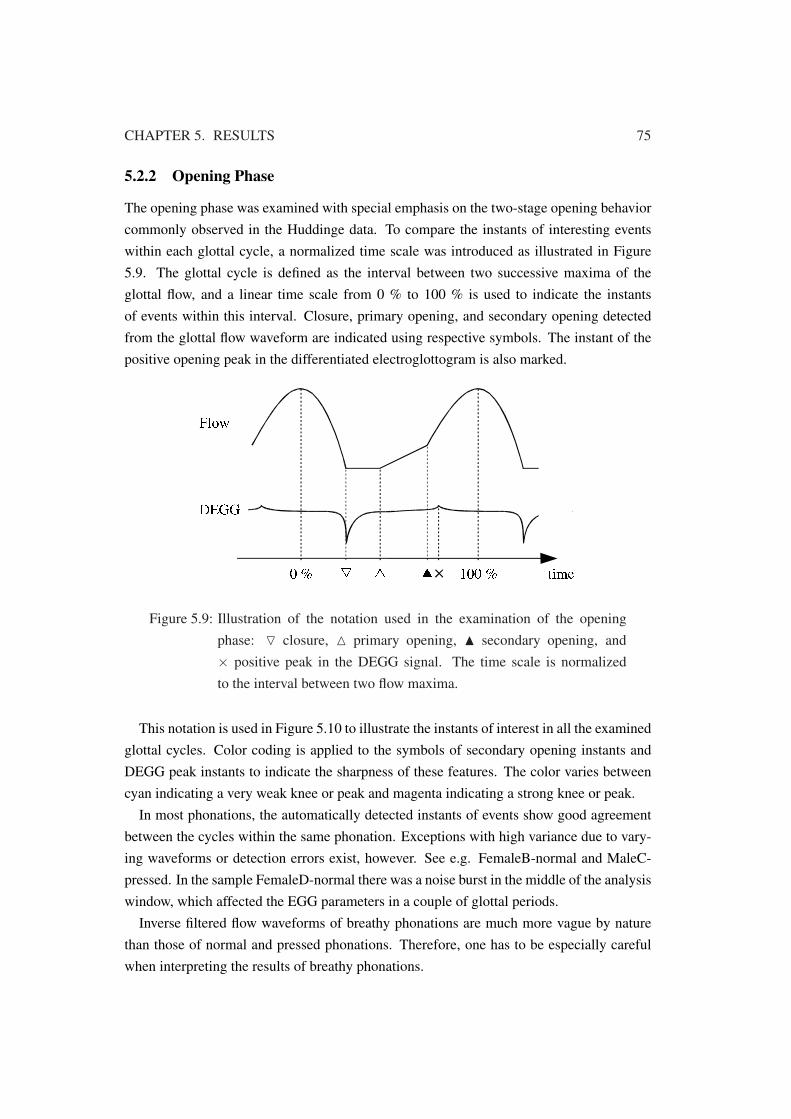
CHAPTER 5. RESULTS 75
5.2.2 Opening Phase
The opening phase was examined with special emphasis on the two-stage opening behaviorcommonly observed in the Huddinge data. To compare the instants of interesting eventswithin each glottal cycle, a normalized time scale was introduced as illustrated in Figure5.9. The glottal cycle is defined as the interval between two successive maxima of theglottal flow, and a linear time scale from 0 % to 100 % is used to indicate the instantsof events within this interval. Closure, primary opening, and secondary opening detectedfrom the glottal flow waveform are indicated using respective symbols. The instant of thepositive opening peak in the differentiated electroglottogram is also marked.
Figure 5.9: Illustration of the notation used in the examination of the openingphase: O closure, M primary opening, N secondary opening, and× positive peak in the DEGG signal. The time scale is normalizedto the interval between two flow maxima.
This notation is used in Figure 5.10 to illustrate the instants of interest in all the examinedglottal cycles. Color coding is applied to the symbols of secondary opening instants andDEGG peak instants to indicate the sharpness of these features. The color varies betweencyan indicating a very weak knee or peak and magenta indicating a strong knee or peak.
In most phonations, the automatically detected instants of events show good agreementbetween the cycles within the same phonation. Exceptions with high variance due to vary-ing waveforms or detection errors exist, however. See e.g. FemaleB-normal and MaleC-pressed. In the sample FemaleD-normal there was a noise burst in the middle of the analysiswindow, which affected the EGG parameters in a couple of glottal periods.
Inverse filtered flow waveforms of breathy phonations are much more vague by naturethan those of normal and pressed phonations. Therefore, one has to be especially carefulwhen interpreting the results of breathy phonations.

CHAPTER 5. RESULTS 76
In many cases, especially in the normal phonations of the male subjects, the instant ofprimary opening occurs very shortly after the closure. This suggests a flow waveform witha very short flat segment followed by a long, gently rising phase.
Some other cases show a very short distance between the primary and secondary opening,see e.g. FemaleA-breathy and MaleB-pressed. This indicates that the detection algorithmdid not find any secondary knee at a later position in the opening phase.
Phonations with strong secondary opening knees and sharp DEGG opening peaks showgood agreement between the instants of these phenomena. Strongest evidence of this isfound in normal phonations of the male subjects A to D and pressed phonations of all malesubjects except Male E.

CHAPTER 5. RESULTS 77
0 25 50 75 100
female A
female B
female C
female D
female E
female F
male A
male B
male C
male D
male E
male F
male G
Breathy
% of cycle
0 25 50 75 100
Normal
% of cycle
0 25 50 75 100
Pressed
% of cycle
0 Sharpness of secondary opening 3
0 Sharpness of DEGG peak 4
Figure 5.10: Significant instants detected from each glottal cycle: O closure, M pri-mary opening, N secondary opening, and × positive peak in DEGG.Time scale is normalized to the glottal cycle length between two suc-cessive flow maxima. Figure 5.9 illustrates the notation. Each rowrefers to one glottal cycle. Color coding indicates the sharpness ofeach DEGG peak and secondary opening knee in the flow waveform.

CHAPTER 5. RESULTS 78
5.2.3 Closing Phase
The behavior of the glottal flow and the electroglottogram during the closing phase wasstudied using the normalized time scale illustrated in Figure 5.11. The instant of maximumflow is used as the origin and the instant of closure determines the 100 % point.
Figure 5.11: The definition of the time scale of the closing phase that will be usedin subsequent illustrations. The instant of maximum flow determinesthe zero position and the instant of closure defines the 100 percentposition.
Figure 5.12 illustrates the instant of the minimum in the flow derivative, or maximumexcitation, and the instant of the negative closing peak in the differentiated EGG waveformin each examined glottal cycle.
It should be pointed out that the inverse filtered flow waveforms of breathy phonationsand the time instants derived from them are less reliable than those acquired from the normaland pressed phonations. This can also be seen in Figure 5.12 as a higher variability of thedetected instants.
The phonation FemaleC-pressed seems to deviate from the common pattern apparentin the column of pressed phonations. Visual examination of the waveforms revealed thatthe flow pulses of FemaleC-pressed showed a smooth closure whereas most other normaland pressed flow pulses had a very abrupt closure. This has shifted the detected instant ofclosure in FemaleC-pressed forward relative to the point of maximum excitation. A smoothclosure of the flow waveform also causes the relatively early instants detected from thephonations FemaleC-normal and FemaleB-pressed.

CHAPTER 5. RESULTS 79
25 50 75 100 125
female A
female B
female C
female D
female E
female F
male A
male B
male C
male D
male E
male F
male G
Breathy
% of closing phase
25 50 75 100 125
Normal
% of closing phase
25 50 75 100 125
Pressed
% of closing phase
Figure 5.12: Positions of minima in flow derivative and closing peaks in DEGGduring the closing phase. Each row indicates the instants of the mini-mum of flow derivative (H) and the negative DEGG peak ( ) withinone glottal cycle. The horizontal axis denotes the time scale of theclosing phase as shown in Figure 5.11.

CHAPTER 5. RESULTS 80
The position of the minimum in the differentiated flow waveform within the closing phasewas examined in more detail. Figure 5.13 shows the average position of this instant for eachsubject and phonation mode separately. The uncertainty of each mean value is indicated bythe 95 % confidence interval derived from the standard error of the mean (SEM), see Section4.3.6 for details. The use of SEM for this small number of samples requires the assumptionof normal distribution. In this case, that seems to be a reasonable approximation.
0
25
50
75
100
fem
ale
Afe
mal
e B
fem
ale
Cfe
mal
e D
fem
ale
Efe
mal
e F
mal
e A
mal
e B
mal
e C
mal
e D
mal
e E
mal
e F
mal
e G
% o
f cl
osin
g ph
ase
Figure 5.13: Position of the minimum flow derivative within the closing phase. Thevertical axis denotes the time scale of the closing phase as shown inFigure 5.11. Breathy phonation is drawn in red, normal phonationin black, and pressed phonation in blue. Vertical lines indicate 95 %confidence intervals derived from the measurements.
No clear trends can be seen in Figure 5.13 except that the maximum excitation occurs inmost cases during the last 25 % of the closing phase.
Finally, the relative timing of the minima in the flow derivative and the EGG derivativewas studied. Figure 5.14 illustrates the time difference ∆t that was measured from eachglottal cycle. The average time difference for every subject and phonation mode is shownin Figure 5.15 in milliseconds and in Figure 5.16 using the time scale normalized to theclosing phase length as illustrated in Figure 5.11. The uncertainty of each mean value isindicated by the 95 % confidence interval derived from the standard error of the mean. Thetime differences are assumed to be normally distributed.
No general rules can be found to predict how this time difference changes when thepressedness of phonation is increased. However, the difference is positive in all but one

CHAPTER 5. RESULTS 81
Figure 5.14: Time difference between the closing peaks in the differentiated flowwaveform and the differentiated electroglottogram. Positive ∆t indi-cates that the instant of minimum flow derivative precedes the instantof minimum DEGG.
0
1
2
fem
ale
Afe
mal
e B
fem
ale
Cfe
mal
e D
fem
ale
Efe
mal
e F
mal
e A
mal
e B
mal
e C
mal
e D
mal
e E
mal
e F
mal
e G
ms
Figure 5.15: Time difference between the minimum of flow derivative and the min-imum of DEGG in milliseconds. Breathy phonation is drawn in red,normal phonation in black, and pressed phonation in blue. Verticallines indicate 95 % confidence intervals derived from the measure-ments.
case. The closing peak in DEGG thus seems to occur after the minimum flow derivative.This hypothesis was tested statistically by performing Student’s t-tests (Laininen, 2000).

CHAPTER 5. RESULTS 82
0
25
50fe
mal
e A
fem
ale
Bfe
mal
e C
fem
ale
Dfe
mal
e E
fem
ale
Fm
ale
Am
ale
Bm
ale
Cm
ale
D
mal
e E
mal
e F
mal
e G
% o
f cl
osin
g ph
ase
Figure 5.16: Time difference between the minimum of flow derivative and the min-imum of DEGG. The time scale is normalized to the closing phaselength, see Figure 5.11. Breathy phonation is drawn in red, normalphonation in black, and pressed phonation in blue. Vertical lines indi-cate 95 % confidence intervals derived from the measurements.
The time difference ∆t was assumed to be normally distributed with unknown variance.The null hypothesis wasH0 : ∆t ≤ 0 and the alternative hypothesis wasH1 : ∆t > 0. Sig-nificance level of 5 % was chosen.
Each phonation mode was tested separately. Furthermore, the test was applied to absolutetime differences in milliseconds, and to time differences normalized by the duration of theclosing phase. P values acquired by the tests are shown in Table 5.6. In each case, theP value was very small and the null hypothesis was rejected at the 5 % significance level.Thus, the maximum excitation in the flow was found to occur before the closing peak in thedifferentiated EGG signal.
Table 5.6: P values obtained from the t-tests of the time difference between theinstants of minimum flow derivative and minimum EGG derivative.
Phonation mode P (difference in ms) P (difference in %)
Breathy 3.3−14 4.7−19
Normal 4.0−22 5.5−26
Pressed 8.9−30 4.5−20

CHAPTER 5. RESULTS 83
5.3 Observations on Inverse Filtering
5.3.1 Primary and Secondary Opening
As remarked in Section 4.3.4, unexpected two-stage opening behavior was often encoun-tered in the inverse filtered glottal flow waveforms. This phenomenon was analyzed quan-titatively by calculating two sets of parameters based on primary and secondary openinginstants.
To further examine the two-stage opening behavior, the phonation Male1-06-normal ofthe Huddinge material was selected for further analysis because it exhibited prominent pri-mary and secondary openings and a clean inverse filtered flow waveform. The microphonesignal of this phonation was inverse filtered using the following two additional methods:
• Inverse filtering based on closed-phase covariance analysis (Wong et al., 1979). Thebeginning of a closed phase of glottal vibration was detected from the derivative of theEGG signal, and a covariance analysis window was located closely after this point.The method was implemented and applied to the signal by professor Paavo Alku.
• Manual inverse filtering using the custom software DeCap developed by SvanteGranqvist (Granqvist et al., 2003). The software allows the operator to adjust man-ually the frequencies and bandwidths of formant filters and displays the resultingflow signal and its spectrum in real time. The test signal was inverse filtered by EvaBjörkner, who is an experienced user of the DeCap software.
Figure 5.17 illustrates the obtained inverse filtered signals together with the original mi-crophone signal, electroglottogram and its derivative, and the glottal area signal estimatedfrom the high-speed image sequence.
The closed-phase covariance analysis gave a flow waveform that is very similar to theone obtained by the IAIF method. Primary and secondary opening instants are evident inthe flow pulses. The glottal flow estimate acquired using the DeCap software also showsdistinct knees at the positions of primary and secondary opening found in the IAIF-basedflow. However, the slope of the DeCap flow signal is different: the flow decreases until thetime instant where the primary opening occurs in the IAIF-based waveform, and notableincrease of flow in the DeCap estimate begins only at the instant of secondary opening inthe IAIF signal. Thus, the DeCap waveform suggests an interpretation that the knee at theinstant of primary opening is caused by some phenomena during the closed phase and thatconsiderable increase of flow does not begin before the instant of secondary opening. Thepeaks of the differentiated EGG signal as well as the area waveform support this view.
It is worth pointing out that the flow waveform given by the IAIF method can be maderesemble the DeCap signal in Figure 5.17 by tuning the lip radiation parameter. The result-

CHAPTER 5. RESULTS 84
0
0
10 msPres
sure
IAIF
CP
DeC
apE
GG
DE
GG
Are
a
Figure 5.17: Comparison of flow waveforms obtained using different inverse fil-tering methods. The figure shows the following signals from top tobottom: original speech pressure signal captured by a microphone,flow waveform obtained using the IAIF method, flow waveform ob-tained by closed-phase covariance analysis, flow waveform obtainedusing the DeCap software, EGG, differentiated EGG, and glottal areaextracted from the high-speed image sequence.
ing waveform thus depends on the preferences of the user of the inverse filtering system.In the IAIF case in the figure, a maximally flat flow waveform after the closure has beenpreferred to a long closed phase.
Figure 5.18 shows another example where the closed phase of the inverse filtered flowwaveform is changed remarkably by modifying inverse filtering parameters. Both flowwaveforms were obtained by inverse filtering the phonation FemaleD-pressed with the HUT

CHAPTER 5. RESULTS 85
IAIF Toolbox software. The high-pass filter cut-off frequency was set to 183 Hz and themaximum number of formants to 11 in both cases. These same parameters were used toinverse filter that phonation for the analysis of the flow waveform in this study. However,the lip radiation parameter was set to two extreme values to get the waveforms in Figure5.18: it was 0.97 in the case (a) and 1.00 in the case (b).
Waveform (b) shows a hump at the beginning of the closed phase. Hertegård et al. (1992)and Hertegård & Gauffin (1995) analyzed this kind of characteristic of the flow waveformand related it to the existence of a mucosal wave, i.e. vertical phase difference along thevocal folds during the closing phase.
Waveform (a), on the other hand, shows a short, flat closed phase and a long openingphase with gradually increasing slope. The shape of the pulses resembles some flow wave-forms with a two-stage opening encountered in this study.
5 ms
Pres
sure
Flow
(a)
Flow
(b)
Figure 5.18: Flow waveforms obtained by inverse filtering a pressed female phona-tion with the IAIF method using two different lip radiation coeffi-cients, 0.97 in (a) and 1.00 in (b). All other parameters were identicalin these two cases.
Speculation arises whether the hump could be more generally converted into a two-phaseopening and vice versa by tuning the inverse filtering parameters, and whether these twocharacteristics of the flow pulse might be caused by the same underlying physiological oracoustical phenomena.

CHAPTER 5. RESULTS 86
Changes in the Flow Waveform
Figure 5.19 illustrates a portion of the phonation Male1-06-breathy. The microphone signalis shown in the top panel, and the two panels below it contain alternative glottal flow esti-mates. Flow (a) is obtained using IAIF with proper high-pass filtering at 101 Hz, maximumnumber of formants 9, and lip radiation coefficient 0.995. Flow (b) is acquired by usingthe same high-pass filtering and setting the maximum number of formants to 7 and the lipradiation coefficient to 0.99.
10 ms
0
Pres
sure
Flow
(a)
Flow
(b)
Are
a
Figure 5.19: Two different flow waveforms (a) and (b) are obtained from the pres-sure signal at the top by using different inverse filtering parameters.The glottal area function is shown for comparison at the bottom.
Flow (a) shows a nearly flat and relatively long closed phase, which in many cases is atypical feature of an expected flow pulse waveform. Flow (b) is almost sinusoidal withoutany flat closed phase. The waveforms differ drastically even though they have both beenachieved using parameter values that are within the range commonly used in this study.
The bottom panel of Figure 5.19 shows the related glottal area signal. Its individual val-ues are not very reliable but it indicates clearly that there was no complete closure duringthese glottal cycles. This observation was verified by visual inspection of the high-speed

CHAPTER 5. RESULTS 87
images. The flat closed phase present in flow (a) is thus not supported by the area func-tion. Furthermore, the flow (a) does not appear to be in phase with the area variation.Consequently, flow (b) seems to be a more plausible estimate of the behavior of the glottalvolume velocity in this breathy phonation than flow (a) even though flow (a) resembles thewaveforms commonly encountered in normal and pressed phonations.
This example illustrates the significance of the choices made by the operator of the in-verse filtering system. It also demonstrates the uncertainty related to the waveforms attainedby inverse filtering and to the pulse parameters derived from those waveforms.
Inability to Achieve a Plausible Flow Waveform
Among the almost one hundred segments of pressure signals that were inverse filteredwithin this study, one signal turned out to be especially problematic for the HUT IAIFToolbox implementation of the IAIF method. When inverse filtering the phonation MaleA-pressed, the software failed to produce a plausible flow waveform. No significant improve-ment was achieved by changing the parameters of the method. Finally, reducing the lengthof the analysis window slightly changed the resulting flow signal into an expected wave-form. Figure 5.20 shows the pressure signal of this phonation, the flow estimate obtainedfrom the entire segment, and the more appropriate flow waveform achieved by leaving ap-proximately one period out at the end of the segment but using exactly the same inversefiltering settings.
Besides, the flow estimate (b) in Figure 5.20 is another example of a flow waveform thatcould have been made to have a hump after the closure and a long, nearly flat closed phaseby tuning the lip radiation coefficient.

CHAPTER 5. RESULTS 88
10 ms
Pres
sure
Flow
(a)
Flow
(b)
Figure 5.20: Problematic signal segment for inverse filtering. The two panels onthe bottom show inverse filtered flow estimates obtained from the mi-crophone signal in the top panel. Flow (a) resulted from inverse filter-ing the entire signal segment, and flow (b) was acquired by reducingthe length of the analysis window by approximately one glottal cycle.All the inverse filtering parameters were identical.

Chapter 6
Conclusions
This chapter concludes the thesis by presenting the most relevant results of the project andrelating them to the results of earlier research. The most interesting detailed findings of thisstudy are also described. Finally, some suggestions are provided that might be useful infuture work within this field.
Due to the nature of this field of research, the results cannot be regarded as exact patternsthat exist uniformly in all examined cases. However, general observations can be foundfrom the material, and interesting details of observed behavior can be pointed out.
6.1 Conclusions about the Inverse Filtering Method
The primary goal of this study was to evaluate the inverse filtering method IAIF by com-paring the flow estimates obtained using it to information attained simultaneously by high-speed imaging and electroglottography. Data collected in the Huddinge experiment pro-vided the possibility of comparing inverse filtered flow waveforms with simultaneouslyrecorded image sequences of the vibrating vocal folds as well as EGG waveforms. Thematerial of the HUT experiment, on the other hand, allowed comparisons between flowand EGG waveforms with more reliable temporal synchronization and better EGG signalquality.
Based on the examined material, it can be stated in general that the inverse filteringmethod produced mostly reasonable estimates of glottal flow waveform.
The user-adjustable parameters of IAIF had a considerable effect on the obtained flowwaveforms. Not all parameter settings gave plausible flow estimates. Therefore, the roleof the operator of the inverse filtering software is crucial. Knowledge and experience onhuman speech production and inverse filtering is required for reliable utilization of theinverse filtering system.
89

CHAPTER 6. CONCLUSIONS 90
The Huddinge material was recorded in a clinical room environment without specificsound-absorbing arrangements. This did not seem to cause problems with inverse filtering.However, the effect of room reflections on the inverse filtered flow waveforms was notexplicitly evaluated in this study.
6.2 Detailed Observations
6.2.1 Incomplete Closure of Vocal Folds
Examination of the high-speed image material of the Huddinge experiment revealed thatthe vocal folds were not completely closed in the breathy phonations of any of the subjects.For the female subject, a minor anterior and posterior gap was commonly encounteredin all but the loudest and most pressed phonations. The male subjects, in general, had acomplete closure in all but the breathy phonations. Hertegård et al. (1992) observed similarbehavior. Their subjects were asked to phonate at different frequencies mostly in the normalphonation mode, and complete closure of vocal folds was found in all phonation samplesof the male subjects but in none of the samples of the female subjects.
6.2.2 Pulse Skewing
Closing quotients of glottal area waveforms were found to be generally greater than thoseof glottal flow pulses. This indicates that the closing phase of the area pulse is longer thanthe closing phase of the corresponding flow pulse, and the flow pulse is thus more skewedto the right. This corroborates earlier theoretical and empirical findings (Rothenberg, 1973,1981a; Stevens, 1998). The acoustic mass of the airways slows down the increase of thevolume velocity when the glottal area is increasing and causes a more rapid decrease of flowin the closing phase (Stevens, 1998). The air displaced by vocal folds may also contributeto the skewing of the flow pulse (Rothenberg, 1973, 1981a).
6.2.3 Flow Waveform in the Closed Phase and the Opening Phase
A two-stage opening phase was commonly encountered in the flow waveforms obtainedin this study. After an abrupt closure, a short, flat closed phase was found, followed by amoderately rising flow segment beginning at the instant of primary opening. At a later pointof time, the flow suddenly started to increase more rapidly. This instant was referred to asthe secondary opening.
Examination of the flow and EGG signals of the HUT experiment showed that the open-ing peak of the differentiated EGG signal often coincided with the automatically detectedinstant of secondary opening in the flow waveform in cases where the DEGG peak and the

CHAPTER 6. CONCLUSIONS 91
secondary opening of flow were evident. Consequently, in waveforms with clear primaryand secondary opening, the secondary opening seemed to correspond to the instant of rapidopening of the vocal folds as detected from the EGG signal. This finding was supportedby visual examination of some phonations of the Huddinge experiment having pronouncedprimary and secondary openings in the flow waveform: the instant of glottal opening, as ob-served visually in the image sequence, occurred near the position of the secondary openingin the flow waveform. The secondary opening thus appeared to be related to the physiolog-ical opening of the vocal folds.
The increase of glottal flow between the primary opening and the secondary openingcould be explained by the piston effect, which means the upward movement of the vocalfolds during the closed phase. Another explanation might be the leakage of air between thevocal folds before a pronounced opening of the vocal folds occurs. Both of these explana-tions have been suggested as reasons for non-zero DC air flow during the closed phase ofthe glottal cycle (Rothenberg, 1973, 1981a; Hertegård et al., 1992).
The two-stage opening phase of the flow waveform could also be caused by slightlyincorrect inverse filtering settings. A case study in Section 5.3.1 showed that tuning the in-tegration coefficient of the inverse filtering method could change the tilt of the closed phaseof the flow signal so that a waveform with a short, flat segment in the beginning of theclosed phase followed by a moderately rising slope was converted into a short segment ofdecreasing flow after the closure followed by a longer, almost horizontal closed phase. Thelatter flow waveform could be described as having a hump in the beginning of the closedphase, and it resembled those observed by Hertegård et al. (1992) and Hertegård & Gauffin(1995). They explained the hump after the closure by a mucosal wave traveling verticallyalong the vocal folds and by the displacement of intraglottal air volume. The signal exam-ined in Section 5.3.1 was particularly suitable for this kind of demonstration, and this resultmay thus not valid in general.
6.2.4 Closing Phase Phenomena
Two characteristics of the glottal closing phase were studied in detail from the HUT record-ings. Firstly, the instant of steepest descent in the glottal flow waveform was located. It wasfound to vary within the last half of the closing phase, most commonly occurring during thelast 25 % of the closing phase. This result is in line with many models of the glottal volumevelocity waveform, including the LF model (Fant et al., 1985), which allow the minimumof the flow derivative to occur at an adjustable point of time before the instant of closure.
Secondly, the time difference between the instants of steepest flow descent and the clos-ing dip in the differentiated EGG waveform was examined. The maximum excitation inthe flow was found to occur before the closing peak in DEGG. This is in agreement with

CHAPTER 6. CONCLUSIONS 92
the observations by Rothenberg (1981b). He stated that the termination of the flow pulse istypically accompanied by the onset of a sharp drop in the EGG waveform, and that the flowpulse terminates closely before the closure of lower vocal fold margins, which is indicatedby the beginning of the steep descent in the EGG waveform. Childers et al. (1983) foundthat the absolute minimum of the differentiated EGG aligned with the instant of glottalclosure. In one of their figures (Childers et al., 1983, page 211), the minimum of differ-entiated volume velocity waveform occurs after the minimum of DEGG, but this may becaused by timing errors of tape recorders also mentioned in their article. In two other fig-ures (Childers et al., 1983, pages 211 and 214), the signal minima seem to be simultaneousor the DEGG minimum occurs slightly later.
6.3 Sources of Error and Uncertainty
6.3.1 Signal Synchronization
In the recordings made in the Huddinge experiment, the synchronization of signals fromdifferent sources appeared to be less accurate than was expected. Comparisons betweenclosure instants detected from microphone, glottal flow, EGG, and area signals suggestedthat the compensation of sound propagation delay from the glottis to the microphone shouldbe smaller than that calculated from the vocal tract length and the microphone distance.This may be partly explained by the experimental setting: Glottal imaging requires that thesubject leans the head forward and the camera operator gently pulls the subject’s tongue.This might cause the effective vocal tract length to be reduced in comparison to a normalspeaking position. At least, it certainly draws the subject’s attention from controlling thedistance between the mouth and the microphone.
The closure instants located in the different signals are not related to exactly the samephysiological events, which may cause some error in this evaluation of synchronizationaccuracy. Some uncertainty was also involved in the alignment of the image sequencerelative to the other signals. However, the time difference between the detected instants ofclosure was larger on average than expected and it consistently suggested that compensationof propagation delay should be smaller.
A similar calculation of sound propagation delay was used by e.g. Baer et al. (1983)and Granqvist et al. (2003). The same compensation scheme also yielded better agreementbetween detectable signs of glottal closure in the flow and EGG signals of the HUT material.
Consequently, the alignment of the signals in the Huddinge material was considered un-reliable to some extent, and detailed temporal comparisons between the signals were notmade on those recordings.

CHAPTER 6. CONCLUSIONS 93
6.3.2 Estimation of Glottal Area
The detection of the area of glottal opening from high-speed image material is far fromtrivial. Even by visual examination, it is often difficult to find the exact position of thevocal fold edges that form the boundaries of the glottal opening. Furthermore, especially inpressed phonations, the visibility to the vocal folds is often limited by supraglottal tissuesthat hide the glottis partially.
An automatic detection algorithm does not provide an ultimate solution to this difficulttask. The High-Speed Toolbox software utilized for automatic area detection in this studyhad problems particularly in finding the edges of the glottis when the opening was narrow.Additionally, in cases with suboptimal illumination, dark areas around the glottis were oftendetected as a part of the glottal opening. The automatically detected area function was alsoaffected by the values of user-adjustable area detection parameters. Therefore, it was foundnecessary to check visually the instants of opening, maximum area, and closure in the imagesequences in order to achieve as accurate parameters of the area pulses as possible.
6.3.3 Time Resolution of High-Speed Image Sequences
The digital high-speed imaging system produced image sequences with approximately 1900frames per second. The fundamental frequency of speech was around 100 Hz in mostphonations of the male subjects, which yielded approximately 20 image frames per glottalcycle or less.
In cases with high fundamental frequency, however, the number of frames per cycle wasmuch smaller. Especially in the loud phonations of the female subject with f0 around300 Hz and OQ approximately 0.5, no more than 3–4 frames were available of the openphase of each cycle. This was obviously not enough for making useful cycle-by-cycleestimates of area pulse parameters from the image data.
Area pulse parameters were determined using the following convention: the instant ofopening was marked at the last frame with no visible opening, and the instant of closurewas set at the first frame showing complete closure. Consequently, the open phase lengthwas likely to be overestimated. This effect was emphasized by low temporal resolution.
Knowing these limitations of the glottal area data, it was essential to consider the errorlimits of the pulse parameters derived from the detected time instants.
An estimate of the glottal area pulse with a larger number of measurement points withina cycle could be achieved by combining the information from several successive cycles.A simple method would be estimating first the fundamental frequency of vibration andshifting a few consecutive area pulses by multiples of the glottal period length to make thepulses overlap in time. This approach was experimented briefly within the study. Due to the
CHAPTER 6. CONCLUSIONS 94
difficulty of defining exactly repeatable area detection criteria, and probably also becauseof varying illumination conditions and differences between successive cycles of vocal foldvibration, overlapping area estimates of consecutive area pulses did not always provide anunambiguous waveform but there were differences between successive pulses. Further-more, this approach has the same inherent limitation as stroboscopy: detailed informationabout the glottal activity during a single cycle is not achieved if the glottal pulse shape isestimated from several cycles.
Assuming accurate estimates of glottal area, it would be possible to estimate the instantof maximum opening at higher time resolution than the sampling interval by interpolatingthe area waveform between the points of highest sample values. The simplest method forpeak interpolation would be fitting a parabola to the three highest sample points and es-timating the peak position and amplitude as the maximum of this parabola. The methodlacks theoretical and physiological relation to vocal fold movement, but might improve theprecision of the position of the area pulse peak.
Some kind of extrapolation scheme would be necessary to improve the temporal preci-sion of instants of opening and closure as well. Linear extrapolation from the two non-zerosamples closest to the opening or closure would be simple but does not seem to yield satis-fying results, especially if the number of samples available from the open phase is small, inwhich case the benefit of extra precision would be greatest.
Better results might be achieved by fitting a model of the glottal area pulse to the obser-vations and estimating the pulse parameters from the model.
6.3.4 Estimation of Pulse Parameters
Pulse parameters were estimated from glottal flow and area signals by locating time instantsof specific events. In this approach, noise in the signals may distort the resulting parametervalues severely, and the sampling frequency also affects the results. Furthermore, manualdetection of such instants may have subjective bias, and automatic implementation of eventdetection easily leads to complex heuristic rules that lack theoretical and physiological ba-sis.
An alternative approach would be to fit a mathematical model to the data and estimateparameters from the fitted model. This would allow estimating amplitudes and time pointsbetween sample values, and the estimates would be more robust (Strik, 1996). A disadvan-tage of this approach is that fitting a predefined model to the data does not allow studyingsignal features that are not included in the chosen model.

CHAPTER 6. CONCLUSIONS 95
6.3.5 Suggestions for Technical Improvements
This section presents a list of practical suggestions that could improve the outcome of asimilar research project in the future.
• The microphone should be fastened to the subject in the recording setting to preventchanges in the microphone distance and to avoid speculations about the microphonedistance as a potential source of synchronization error.
• The quality of the EGG signal should be controlled before and during a recordingsession. If the signal is found to be weak or noisy, adjustments should be made toimprove the signal quality if possible.
• More specific measurements should be carried out to evaluate possible delays andinaccuracies in the Huddinge measurement equipment. This would be necessary toimprove the reliability and to decrease the uncertainty of the synchronization of thedifferent signal sources.
• The algorithm of automatic glottal area detection could be improved to better tracethe glottis when the opening is narrow.
• Methods for improving the time resolution of glottal area function should be consid-ered. A modern camera system would be capable of recording images at a higherframe rate. But with the existing equipment, interpolation methods or utilization ofseveral cycles for determining the pulse shape might improve the temporal precision.
6.4 Concluding Remarks
In this study, an combination of the following three voice analysis methods was utilized:inverse filtering, high-speed imaging, and electroglottography. Information obtained simul-taneously by these methods was used to evaluate the inverse filtering method IAIF. Theresults suggest that IAIF produces reasonable estimates of glottal volume velocity wave-form. However, experience is needed in the inverse filtering task.
The material of this study was also used to examine the behavior of the human voicesource. The glottal flow waveform was found to be more skewed to the right than thecorresponding glottal area pulse, which corroborates the results of earlier studies.
A two-stage opening phase was often encountered in the flow waveforms. In many suchcases, the flow estimate increased from the base level before the opening of the vocal foldswas indicated by high-speed images or the electroglottogram.

CHAPTER 6. CONCLUSIONS 96
Finally, two details of the closing phase were studied. The minimum of the differentiatedglottal flow waveform was found to take place mostly in the last 25 % of the closing phase,and it was also found to occur before the minimum of the differentiated EGG waveform.

Bibliography
Airas, M. (2004), ‘Matsig - an object-oriented signal processing class library forMATLAB’, web page. Referenced 22 December 2004.URL http://matsig.sourceforge.net/
Airas, M. & Alku, P. (2004), ‘Emotions in short vowel segments: Effects of the glottalflow as reflected by the normalized amplitude quotient’, in E. André, L. Dybkjær &W. Minker, eds., ‘Proceedings of Affective Dialogue Systems’, Kloster Irsee, Germany,pp. 13–24.
Alku, P. (1992), ‘Glottal wave analysis with pitch synchronous iterative adaptive inversefiltering’, Speech Communication, vol. 11, pp. 109–119.
Alku, P., Bäckström, T. & Vilkman, E. (2002), ‘Normalized amplitude quotient forparametrization of the glottal flow’, The Journal of the Acoustical Society of America,vol. 112, no. 2, pp. 701–710.
Alku, P., Tiitinen, H. & Näätänen, R. (1999), ‘A method for generating natural-soundingspeech stimuli for cognitive brain research’, Clinical Neurophysiology, vol. 110, pp.1329–1333.
Ananthapadmanabha, T. & Yegnanarayana, B. (1975), ‘Epoch extraction of voiced speech’,IEEE Transactions on Acoustics, Speech, and Signal Processing, vol. ASSP-23, no. 6,pp. 562–570.
Baer, T., Löfqvist, A. & McGarr, N. S. (1983), ‘Laryngeal vibrations: A comparison be-tween high-speed filming and glottographic techniques’, The Journal of the AcousticalSociety of America, vol. 73, no. 4, pp. 1304–1308.
Baken, R. J. (1992), ‘Electroglottography’, Journal of Voice, vol. 6, no. 2, pp. 98–110.
Bäckström, T., Alku, P. & Vilkman, E. (2002), ‘Time-domain parametrization of the clos-ing phase of glottal airflow waveform from voices over a large intensity range’, IEEETransactions on Speech and Audio Processing, vol. 10, no. 3, pp. 186–192.
97
BIBLIOGRAPHY 98
Cheng, Y. M. & O’Shaughnessy, D. (1989), ‘Automatic and reliable estimation of glottalclosure instant and period’, IEEE Transactions on Acoustics, Speech, and Signal Pro-cessing, vol. 37, no. 12, pp. 1805–1815.
Childers, D., Smith, A. & Moore, G. (1984), ‘Relationships between electroglottograph,speech, and vocal cord contact’, Folia Phoniatrica, vol. 36, pp. 105–118.
Childers, D. D., Naik, J. M., Larar, J. N., Krishnamurthy, A. K. & Moore, G. P. (1983),‘Electroglottography, speech, and ultra-high speed cinematography’, in I. R. Titze &R. C. Scherer, eds., ‘Vocal Fold Physiology, Biomechanics, Acoustics and PhonatoryControl’, The Denver Center for The Performing Arts, Denver, pp. 202–220.
Claes, T., Dologlou, I., ten Bosch, L. & Compernolle, D. V. (1998), ‘A novel feature trans-formation for vocal tract length normalization in automatic speech recognition’, IEEETransactions on Speech and Audio Processing, vol. 6, no. 6, pp. 549–557.
Colton, R. H. & Conture, E. G. (1990), ‘Problems and pitfalls of electroglottography’,Journal of Voice, vol. 4, no. 1, pp. 10–24.
de Cheveigné, A. & Kawahara, H. (2002), ‘YIN, a fundamental frequency estimator forspeech and music’, The Journal of the Acoustical Society of America, vol. 111, no. 4, pp.1917–1930.
Doebelin, E. O. (1975), Measurement Systems, Application and Design, McGraw-Hill, re-vised edn.
El-Jaroudi, A. & Makhoul, J. (1991), ‘Discrete all-pole modeling’, IEEE Transactions onSignal Processing, vol. 39, no. 2, pp. 411–423.
Eysholdt, U., Tigges, M., Wittenberg, T. & Pröschel, U. (1996), ‘Direct evaluation of high-speed recordings of vocal fold vibrations’, Folia Phoniatrica et Logopaedica, vol. 48, pp.163–170.
Fabre, P. (1940), ‘Sphygmographie par simple contact d’électrodes cutanées, introduisantdans l’arterè de faibles courants de haute fréquence détecteurs de ses variationsvolumétriques’, Comptes Rendus Soc Biol, vol. 133, pp. 639–641.
Fabre, P. (1957), ‘Un procédé électrique percutané d’inscription de l’accolement glottiqueau cours de la phonation: Glottographie de haute fréquence’, Bulletin de l’AcadémieNationale de Médicine, vol. 141, pp. 66–69.
Fant, G. (1960), Acoustic Theory of Speech Production, Mouton, The Hague.

BIBLIOGRAPHY 99
Fant, G., Liljencrants, J. & Lin, Q. (1985), ‘A four-parameter model of glottal flow’, SpeechTransmission Laboratory Quarterly Progress and Status Report (STL-QPSR), Royal In-stitute of Technology, Stockholm, vol. 4, pp. 1–13.
Farnsworth, D. (1940), ‘High-speed motion pictures of the human vocal cords’, Bell Labo-ratories Record, vol. 18, pp. 203–208.
Flanagan, J. L. (1972), Speech Analysis Synthesis and Perception, Springer-Verlag, secondedn.
Fritzell, B. (1992), ‘Inverse filtering’, Journal of Voice, vol. 6, no. 2, pp. 111–114.
Gobl, C. & Chasaide, A. N. (2003), ‘The role of voice quality in communicating emotion,mood and attitude’, Speech Communication, vol. 40, no. 1–2, pp. 189–212.
Granqvist, S., Hertegård, S., Larsson, H. & Sundberg, J. (2003), ‘Simultaneous analysisof vocal fold vibration and transglottal airflow; exploring a new experimental setup’,Speech, Music and Hearing, Quarterly Progress and Status Report (TMH-QPSR), RoyalInstitute of Technology, Stockholm, vol. 45, pp. 35–46.
Henrich, N., d’Alessandro, C., Doval, B. & Castellengo, M. (2004), ‘On the use of thederivative of electroglottographic signals for characterization of nonpathological phona-tion’, The Journal of the Acoustical Society of America, vol. 115, no. 3, pp. 1321–1332.
Hertegard, S. & Gauffin, J. (1992), ‘Acoustic properties of the rothenberg mask’, SpeechTransmission Laboratory Quarterly Progress and Status Report (STL-QPSR), Royal In-stitute of Technology, Stockholm, vol. 2–3, pp. 9–18.
Hertegård, S. & Gauffin, J. (1995), ‘Glottal area and vibratory patterns studied with simul-taneous stroboscopy, flow glottography, and electroglottography’, Journal of Speech andHearing Research, vol. 38, pp. 85–100.
Hertegård, S., Gauffin, J. & Karlsson, I. (1992), ‘Physiological correlates of the inversefiltered flow waveform’, Journal of Voice, vol. 6, no. 3, pp. 224–234.
Hertegård, S., Gauffin, J. & Åke Lindestad, P. (1995), ‘A comparison of subglottal andintraoral pressure measurements during phonation’, Journal of Voice, vol. 9, pp. 149–155.
Hertegård, S., Larsson, H. & Wittenberg, T. (2003), ‘High-speed imaging: applications anddevelopment’, Logopedics Phoniatrics Vocology, vol. 28, pp. 133–139.

BIBLIOGRAPHY 100
Holmberg, E., Hillman, R. & Perkell, J. (1988), ‘Glottal airflow and transglottal air pressuremeasurements for male and female speakers in soft, normal, and loud voice’, The Journalof the Acoustical Society of America, vol. 84, no. 2, pp. 511–529.
Holmes, J. (1962), ‘An investigation of the volume velocity waveform at the larynx duringspeech by means of an inverse filter’, in ‘Proceedings of the 4th International Congresson Acoustics’, Copenhagen.
Hunt, M. J., Bridle, J. S. & Holmes, J. N. (1978), ‘Interactive digital inverse filtering andits relation to linear prediction methods’, in ‘Proceedings of the IEEE International Con-ference on Acoustics, Speech, and Signal Processing (ICASSP ’78)’, vol. 3, pp. 15–18.
Javkin, H. R., Antonanzas-Barroso, N. & Maddieson, I. (1987), ‘Digital inverse filtering forlinguistic research’, Journal of Speech and Hearing Research, vol. 30, pp. 122–129.
Karjalainen, M. (2000), Kommunikaatioakustiikka, Otamedia Oy.
Kiritani, S., Honda, K., Imagawa, H. & Hirose, H. (1986), ‘Simultaneous high-speed dig-ital recording of vocal fold vibration and speech signal’, in ‘Proceedings of the IEEEInternational Conference on Acoustics, Speech, and Signal Processing’, vol. 11, Tokyo,Japan, pp. 1633–1636.
Kiritani, S., Imagawa, H. & Hirose, H. (1990), ‘Vocal cord vibration and voice sourcecharacteristics – observations by a high-speed digital recording’, in ‘Proceedings of theInternational Conference on Spoken Language Processing (ICSLP ’90)’, Kobe, Japan,pp. 61–64.
Klaucke, D., Sunderland, N., Gogstad, E. & Wren, S. (2004), ‘Standard deviation andstandard error of the mean’, web page. Referenced 24 January 2005.URL http://www.cdc.gov/epo/dih/MiniModules/sd_sem/page01.htm
Krishnamurthy, A. & Childers, D. (1981), ‘Vocal fold vibratory patterns: Comparisonof film and inverse filtering’, in ‘Proceedings of the IEEE International Conference onAcoustics, Speech, and Signal Processing (ICASSP ’81)’, vol. 6, pp. 133–136.
Laininen, P. (2000), Tilastollisen analyysin perusteet, 597, Otatieto, Helsinki, second edn.
Larsson, H., Hertegård, S., Lindestad, P. & Hammarberg, B. (2000), ‘Vocal fold vibrations:High-speed imaging, kymography, and acoustic analysis: A preliminary report’, TheLaryngoscope, vol. 110, pp. 2117–2122.
Laukkanen, A.-M. & Leino, T. (1999), Ihmeellinen ihmisääni, Gaudeamus.

BIBLIOGRAPHY 101
Lauri, E.-R., Alku, P., Vilkman, E., Sala, E. & Sihvo, M. (1997), ‘Effects of prolonged oralreading on time-based glottal flow waveform parameters with special reference to genderdifferences’, Folia Phoniatrica et Logopaedica, vol. 49, pp. 234–246.
Lecluse, F., Brocaar, M. & Verschuure, J. (1975), ‘The electroglottography and its relationto glottal activity’, Folia Phoniatrica, vol. 27, pp. 215–224.
Lehto, L., Airas, M., Björkner, E., Sundberg, J. & Alku, P. (2005), ‘Comparison of twoinverse filtering methods for determining the normalized amplitude quotient and closingquotient - voice source characteristics in different phonation types’, Journal of Voice.Manuscript in preparation.
Ma, C., Kamp, Y. & Willems, L. F. (1994), ‘A frobenius norm approach to glottal closuredetection from the speech signal’, IEEE Transactions on Speech and Audio Processing,vol. 2, no. 2, pp. 258–265.
Marasek, K. (1997), ‘EGG & voice quality’, web page. Referenced 20 December 2004.URL http://www.ims.uni-stuttgart.de/phonetik/EGG/
Markel, J. E. & Gray, A. (1976), Linear Prediction of Speech, Springer-Verlag.
Merriam-Webster (2004), ‘Merriam-Webster OnLine’, web page. Referenced 30 November2004.URL http://www.webster.com/
Miller, R. (1959), ‘Nature of the vocal cord wave’, The Journal of the Acoustical Society ofAmerica, vol. 31, no. 6, pp. 667–677.
Owens, R. (1997), ‘Classical feature detection’, web page. Referenced 23 December 2004.URL http://homepages.inf.ed.ac.uk/rbf/CVonline/LOCAL_COPIES/
OWENS/LECT6/node2.html
Pindyck, R. S. & Rubinfeld, D. L. (1998), Econometric Models and Economic Forecasts,McGraw-Hill, fourth edn.
Rabiner, L. R. & Gold, B. (1975), Theory and Application of Digital Signal Processing,Prentice-Hall.
Rosenberg, A. E. (1971), ‘Effect of glottal pulse shape on the quality of natural vowels’,The Journal of the Acoustical Society of America, vol. 49, no. 2, pp. 583–590.
Rothenberg, M. (1973), ‘A new inverse-filtering technique for deriving the glottal air flowwaveform during voicing’, The Journal of the Acoustical Society of America, vol. 53,no. 6, pp. 1632–1645.

BIBLIOGRAPHY 102
Rothenberg, M. (1981a), ‘Acoustic interaction between the glottal source and the vocaltract’, in K. Stevens & M. Hirano, eds., ‘Vocal fold physiology’, University of TokyoPress, Tokyo, pp. 305–323.
Rothenberg, M. (1981b), ‘Some relations between glottal air flow and vocal fold contactarea’, in C. Ludlow & M. Hart, eds., ‘Proceeding of the conference on the assessment ofvocal pathology’, vol. 11, American Speech-Language-Hearing Association, Rockville,MD, pp. 88–96.
Sakakibara, K.-I., Imagawa, H., Konishi, T., Kondo, K., Murano, E. Z., Kumada, M. & Ni-imi, S. (2001), ‘Vocal fold and false vocal fold vibrations in throat singing and synthesisof khöömei’, in ‘Proceedings of the International Computer Music Conference 2001’,International Computer Music Association, pp. 135–138.
Sakakibara, K.-I., Kimura, M., Imagawa, H., Niimi, S. & Tayama, N. (2004), ‘Physiolog-ical study of the supraglottal structure’, in ‘Proceedings of the International Conferenceon Voice Physiology and Biomechanics’, Association de Formation et de Recherche enOrthophonie Phoniatrie.
Scarborough, J. (1955), Numerical Mathematical Analysis, The Johns Hopkins Press, Bal-timore, 3rd edn.
Scherer, R. C., Druker, D. G. & Titze, I. R. (1988), ‘Electroglottography and direct mea-surement of vocal fold contact area’, in O. Fujimora, ed., ‘Vocal Physiology: Voice Pro-duction, Mechanisms and Functions’, Raven Press, New York, pp. 279–291.
Schutte, H. K. & Miller, D. G. (2001), ‘Measurement of closed quotient in a female singingvoice by electroglottography and videokymography’, in ‘Proceedings of the 5th Inter-national Conference on Advances in Quantitative Laryngoscopy, Voice and Speech Re-search’, Groningen.
Smits, R. & Yegnanarayana, B. (1995), ‘Determination of instants of significant excitationin speech using group delay function’, IEEE Transactions of Speech and Audio Process-ing, vol. 3, no. 5.
Stevens, K. N. (1998), Acoustic Phonetics, The MIT Press.
Story, B. H. (2002), ‘An overview of the physiology, physics and modeling of the soundsource for vowels’, Acoustical Science and Technology, vol. 23, no. 4, pp. 195–206.
Strik, H. (1996), ‘Comments on “Effects of bandwidth on glottal airflow waveforms esti-mated by inverse filtering” [J. Acoust. Soc. Am. 98, 763–767 (1995)]’, The Journal ofthe Acoustical Society of America, vol. 100, no. 2, pp. 1246–1249.

BIBLIOGRAPHY 103
Strik, H. (1998), ‘Automatic parametrization of differentiated glottal flow: Comparingmethods by means of synthetic flow pulses’, The Journal of the Acoustical Society ofAmerica, vol. 103, no. 5, pp. 2659–2669.
Strube, H. W. (1974), ‘Determination of the instant of glottal closure from the speech wave’,The Journal of the Acoustical Society of America, vol. 56, no. 5, pp. 1625–1629.
Švec, J. G. & Schutte, H. K. (1996), ‘Videokymography: High-speed line scanning of vocalfold vibration’, Journal of Voice, vol. 10, no. 2, pp. 201–205.
Södersten, M., Håkansson, A. & Hammarberg, B. (1999), ‘Comparison between automaticand manual inverse filtering procedures for healty female voices’, Logopedics Phoni-atrics Vocology, vol. 24, pp. 26–38.
The MathWorks (2004), ‘Matlab R©7.0.1’, web page. Referenced 22 December 2004.URL http://www.mathworks.com/products/matlab/
Titze, I. R. (1990), ‘Interpretation of the electroglottographic signal’, Journal of Voice,vol. 4, no. 1, pp. 1–9.
Titze, I. R. (1994), Principles of Voice Production, Prentice-Hall.
Titze, I. R., Story, B. H., Burnett, G. C., Holzrichter, J. F., Ng, L. C. & Lea, W. A. (2000),‘Comparison between electroglottography and electromagnetic glottography’, The Jour-nal of the Acoustical Society of America, vol. 107, no. 1, pp. 581–588.
Vaari, J. (1994), Fysiikan laboratoriotyöt, Suomen Fyysikkoseura, Jyväskylä.
Veldhuis, R. (1998), ‘A computationally efficient alternative for the Liljencrants–Fantmodel and its perceptual evaluation’, The Journal of the Acoustical Society of America,vol. 103, no. 1, pp. 566–571.
Vilkman, E., Lauri, E.-R., Alku, P., Sala, E. & Sihvo, M. (1997), ‘Loading changes in time-based parameters of glottal flow waveforms in different ergonomic conditions’, FoliaPhoniatrica et Logopaedica, vol. 49, pp. 247–263.
Weinberger Vision (2004), ‘Weinberger vision’, web page. Referenced 23 December 2004.URL http://www.weinbergervision.com/
Wittenberg, T., Bloss, H., Gick, S., Heppner, W., Tigges, M., Popp, I. & Schmidt, R.(2001), ‘Some thoughts about color-high-speed-cameras’, in ‘Proceedings of the 5th In-ternational Conference on Advances in Quantitative Laryngoscopy, Voice and SpeechResearch’, Groningen.

BIBLIOGRAPHY 104
Wittenberg, T., Tigges, M., Spinnler, K. & Eysholdt, U. (2000), ‘Some thoughts about3D and stereo in laryngoscopy’, in ‘Proceedings of the 4th International Workshop onAdvances in Quantitative Laryngoscopy, Voice and Speech Research’, Jena, pp. 116–123.
Wong, D. Y., Markel, J. D. & Gray, A. H. (1979), ‘Least squares glottal inverse filteringfrom the acoustic speech waveform’, IEEE Transactions on Acoustics, Speech, and Sig-nal Processing, vol. ASSP-27, no. 4, pp. 350–355.

Appendix A
Huddinge Data
This appendix contains graphical illustrations of the pulse parameters derived from all ex-amined flow and area pulses of the Huddinge material. Parameters are shown with errorbounds that indicate the uncertainty due to limited time resolution.
For each examined sequence of five consecutive glottal periods, the inverse filtered flowwaveform and the area pulse of the third of the five cycles are also shown. The flow and areapulses thus originate from the same glottal cycle, but they are not synchronized accuratelyin these illustrations.
In some cases, the area waveforms show obvious errors that are caused by incorrecttracing of the vocal fold edges by the automatic detection algorithm. Additionally, manyindividual area values were modified manually by tuning the area detection parameters forthose image frames. This was done primarily in order to make the maximum of each areapulse coincide with the image frame that indicated maximum opening by visual inspection.In addition, the instants of opening and closure in the area waveforms were treated similarlyto make them agree better with visual observations. This tuning of individual area valuesoccasionally caused noticeable discontinuities in the overall pulse shapes. Consequently,the area pulses adjusted with this procedure cannot always be considered fully reliable.
Due to obvious detection errors and especially the inability of the area estimation soft-ware to detect very narrow openings, the area pulse parameters were, after all, calculatedfrom manually marked instants of opening, maximum area, and closure. Thus, the parame-ters are not directly based on the area waveforms.
105

APPENDIX A. HUDDINGE DATA 106
100
120
0.8
1
0.4
0.6
0.51
1.5
Male1−03 Male1−03Male1−05 Male1−05Male1−06 Male1−06Male1−07 Male1−07Flow Area
f 0 / H
zO
QC
lQS
QP
ulse
s
100
110
120
0.6
0.8
0.2
0.3
0.4
123
Male1−03 Male1−03Male1−05 Male1−05Male1−06 Male1−06Male1−07 Male1−07Flow Area
f 0 / H
zO
QC
lQS
QP
ulse
s
100110120
0.4
0.6
0.8
0.1
0.2
0.3
12345
Male1−03 Male1−03Male1−05 Male1−05Male1−06 Male1−06Male1−07 Male1−07Flow Area
f 0 / H
zO
QC
lQS
QP
ulse
s
Figure A.1: Parameters estimated from breathy (top), normal (middle), and pressed(bottom) phonations of the subject Male 1. Each column with fivevalues of each parameter corresponds to one recording from which fivesuccessive glottal periods have been analyzed. For OQ and SQ, cross(×) denotes primary opening and dot (•) denotes secondary opening.Vertical lines indicate estimated error boundaries due to limited timeresolution. A sample pulse is shown for each phonation.

APPENDIX A. HUDDINGE DATA 107
859095
100105
0.95
1
1.05
0.4
0.6
0.5
1
1.5
Male2−12 Male2−12Male2−13 Male2−13Male2−14 Male2−14Male2−15 Male2−15Flow Area
f 0 / H
zO
QC
lQS
QP
ulse
s
90
100
110
0.50.60.70.80.9
0.150.2
0.250.3
0.35
123
Male2−12 Male2−12Male2−13 Male2−13Male2−14 Male2−14Male2−15 Male2−15Flow Area
f 0 / H
zO
QC
lQS
QP
ulse
s
90
100
0.40.60.8
0.1
0.2
0.3
2
4
Male2−12 Male2−12Male2−13 Male2−13Male2−14 Male2−14Male2−15 Male2−15Flow Area
f 0 / H
zO
QC
lQS
QP
ulse
s
Figure A.2: Parameters estimated from breathy (top), normal (middle), and pressed(bottom) phonations of the subject Male 2. Each column with five val-ues for each parameter corresponds to one recording from which fivesuccessive glottal periods have been analyzed. For OQ and SQ, cross(×) denotes primary opening and dot (•) denotes secondary opening.Vertical lines indicate estimated error boundaries due to limited timeresolution. A sample pulse is shown for each phonation.

APPENDIX A. HUDDINGE DATA 108
150160170180190
0.8
1
0.4
0.6
0.5
1
1.5
Female1−38 Female1−38Female1−39 Female1−39Female1−40 Female1−40Flow Area
f 0 / H
zO
QC
lQS
QP
ulse
s
150160170180190
0.6
0.8
0.2
0.4
123
Female1−38 Female1−38Female1−39 Female1−39Female1−40 Female1−40Flow Area
f 0 / H
zO
QC
lQS
QP
ulse
s
160180200
0.4
0.6
0.2
0.4
0123
Female1−38 Female1−38Female1−39 Female1−39Female1−40 Female1−40Flow Area
f 0 / H
zO
QC
lQS
QP
ulse
s
Figure A.3: Parameters estimated from breathy (top), normal (middle), and pressed(bottom) phonations of the subject Female 1. Each column with fivevalues of each parameter corresponds to one recording from which fivesuccessive glottal periods have been analyzed. For OQ and SQ, cross(×) denotes primary opening and dot (•) denotes secondary opening.Vertical lines indicate estimated error boundaries due to limited timeresolution. A sample pulse is shown for each phonation.

APPENDIX A. HUDDINGE DATA 109
100
120
140
0.4
0.6
0.8
0.150.2
0.250.3
0.35
123
Male1−08 Male1−08Male1−09 Male1−09Male1−10 Male1−10Flow Area
f 0 / H
zO
QC
lQS
QP
ulse
s
140160180
0.4
0.6
0.20.30.4
0.51
1.52
2.5
Male1−08 Male1−08Male1−09 Male1−09Male1−10 Male1−10Flow Area
f 0 / H
zO
QC
lQS
QP
ulse
s
180200220240260
0.4
0.6
0.8
0.2
0.4
0123
Male1−08 Male1−08Male1−09 Male1−09Male1−10 Male1−10Flow Area
f 0 / H
zO
QC
lQS
QP
ulse
s
Figure A.4: Parameters estimated from soft (top), normal (middle), and loud (bot-tom) phonations of the subject Male 1. Each column with five valuesof each parameter corresponds to one recording from which five suc-cessive glottal periods have been analyzed. For OQ and SQ, cross(×) denotes primary opening and dot (•) denotes secondary opening.Vertical lines indicate estimated error boundaries due to limited timeresolution. A sample pulse is shown for each phonation.

APPENDIX A. HUDDINGE DATA 110
100
120
0.50.60.70.80.9
0.150.2
0.250.3
0.35
123
Male2−16 Male2−16Male2−17 Male2−17Male2−18 Male2−18Flow Area
f 0 / H
zO
QC
lQS
QP
ulse
s
120
140
160
0.4
0.6
0.8
0.150.2
0.250.3
0.35
2
4
Male2−16 Male2−16Male2−17 Male2−17Male2−18 Male2−18Flow Area
f 0 / H
zO
QC
lQS
QP
ulse
s
150
200
0.4
0.6
0.10.20.3
0
2
4
Male2−16 Male2−16Male2−17 Male2−17Male2−18 Male2−18Flow Area
f 0 / H
zO
QC
lQS
QP
ulse
s
Figure A.5: Parameters estimated from soft (top), normal (middle), and loud (bot-tom) phonations of the subject Male 2. Each column with five valuesof each parameter corresponds to one recording from which five suc-cessive glottal periods have been analyzed. For OQ and SQ, cross(×) denotes primary opening and dot (•) denotes secondary opening.Vertical lines indicate estimated error boundaries due to limited timeresolution. A sample pulse is shown for each phonation.

APPENDIX A. HUDDINGE DATA 111
150
200
0.6
0.8
0.2
0.4
123
Female1−41 Female1−41Female1−42 Female1−42Female1−43 Female1−43Flow Area
f 0 / H
zO
QC
lQS
QP
ulse
s
200250300
0.40.60.8
0.2
0.4
0.6
0123
Female1−41 Female1−41Female1−42 Female1−42Female1−43 Female1−43Flow Area
f 0 / H
zO
QC
lQS
QP
ulse
s
250300350400450
0.5
1
0.20.40.6
0123
Female1−41 Female1−41Female1−42 Female1−42Female1−43 Female1−43Flow Area
f 0 / H
zO
QC
lQS
QP
ulse
s
Figure A.6: Parameters estimated from soft (top), normal (middle), and loud (bot-tom) phonations of the subject Female 1. Each column with five val-ues of each parameter corresponds to one recording from which fivesuccessive glottal periods have been analyzed. For OQ and SQ, cross(×) denotes primary opening and dot (•) denotes secondary opening.Vertical lines indicate estimated error boundaries due to limited timeresolution. A sample pulse is shown for each phonation.