analysis of l-band multi-channel sea clutter · analysis of l-band multi-channel sea clutter yunhan...
TRANSCRIPT

Analysis of L-band Multi-Channel Sea Clutter
Yunhan Dong and David Merrett
Electronic Warfare and Radar Division Defence Science and Technology Organisation
DSTO-TR-2455
ABSTRACT An L-band multi-channel sea clutter trial was conducted using a DSTO-built 16-channel receiving array (called XPAR) in May 2008 at Kangaroo Island, South Australia. This report presents a number of calibration techniques and analyses various properties of sea clutter including backscatter coefficient, spatial and temporal correlations, distributions and Doppler spectra. Observed phenomena are explained.
RELEASE LIMITATION
Approved for public release

Published by Electronic Warfare and Radar Division DSTO Defence Science and Technology Organisation PO Box 1500 Edinburgh South Australia 5111 Australia Telephone: (08) 7389 5555 Fax: (08) 7389 6567 © Commonwealth of Australia 2010 AR-014-829 August 2010 APPROVED FOR PUBLIC RELEASE
Analysis of L-band Multi-Channel Sea Clutter
Executive Summary In support of SEA1448, the ANZAC Anti-Ship Missile Defence (ASMD) program, the Microwave Radar Branch of Electronic Warfare and Radar Division of DSTO built an L-band phased 16-channel receiving array (called XPAR) and collected its first sea clutter in a trial conducted on 12-17 May 2008 at Kangaroo Island, South Australia. This report presents the processing and analysis of two vertically polarised sea clutter datasets collected during the trial. Calibration is critical to the quality of sea clutter data. XPAR calibration used a calibration dwell collected prior to the data dwell, and was carried out in three steps:
1. Amplitude calibration for uncompressed signal;
2. Phase calibration for uncompressed signal; and
3. Calibration of compressed signal. This calibration technique was found to be very effective and result in satisfactory calibration. It was identified that the data dwell was contaminated by interference due to the noise floor of the transmitter (the transmitter was not switched off during receiving). The interference signal can be modelled to consist of two components. One is a constant component dependent on channels but independent of pulses and range bins. The other is a Gaussian distributed random noise varying with pulses and range bins that is coupled to channels of XPAR with different coupling coefficients. The constant component has been estimated and removed from the data. The Gaussian component has also been estimated but could not be removed from the sea clutter data due to its nature of randomly varying from range bin to range bin and pulse to pulse. The existence of this Gaussian interference noise lifts the noise floor of the receiver (the lift can be as large as 8–10 dB in some channels) and reduces the clutter to noise ratio especially for far range bins. With regard to sea clutter analysis, we have made the following observations:
The measured backscatter coefficients of sea clutter are in good agreement with published values.
Sea clutter intensity at low grazing angle normally reduces at a rate faster than 4r where r is the range. The decrease in sea clutter intensity against range is found not only to vary with range but is also dependent on weather and sea surface conditions. The decrease is slower if the sea surface is rougher with higher sea waves. In contrast, a smoother sea surface with lower sea waves leads to a faster decrease.

The azimuth pattern of sea clutter is sinusoidal with its peak and trough approximately in the upwind and crosswind directions, respectively. The difference between the two is about 6–7 dB. The dataset collected in the downwind direction, however, does not show an obvious peak or trough in the downwind direction.
It has been demonstrated that the sea clutter collected by a floodlight transmitter and a multi-channel array is less spiky than what would be collected by a traditional single-aperture radar with pencil beams in transmit and receive. The difference lies in the beamwidth of the transmitter. The floodlight transmitter illuminates a wider angular region of sea surface and hence more sidelobe clutter power returns to average in the pencil beam receiver, than the sidelobe clutter received for a pencil-beam transmitter.
The spatial distribution of sea clutter is K-distributed. For the first dataset, the shape parameter varies from 1.5 to 7.5, with the smallest (spikiest sea clutter) and largest (least spiky) shape parameters approximately aligning with the crosswind and upwind directions, respectively. The analysis of the second dataset shows the shape parameter varies from 8.5 aligning with the downwind direction to either smaller or larger in other directions.
In general sea clutter with range separation greater than the radar’s range resolution is spatially uncorrelated. Similarly, sea clutter with azimuth separation greater than the radar’s azimuth resolution is also spatially uncorrelated. Long-term spatial correlation reveals sea wave structures in range. A detailed study will be difficult, as the correlation is dependent on the number of samples used in the averaging processing. The oscillation of correlation coefficients gradually fades with an increase in the number of samples used in the averaging processing.
The temporal correlation time of sea clutter is dependent on the environmental parameters. The mean correlation time is about 20 ms for the first dataset (with a sea state about 4) and longer than 100 ms for the second dataset (with a sea state about 3). Sea clutter in the upwind direction and crosswind directions tends to have a longer correlation time.
The temporal distribution of sea clutter is Rayleigh (for amplitude distribution) or exponential (for intensity distribution). If the observation time is short and only in the order of or a few multiples of correlation time, the mean may not be estimated accurately, and the resultant distribution appears to be narrower than the Rayleigh distribution. It is anticipated that if the observation time is of the order of seconds, the distribution would be Rayleigh. If the observation time is very long and on the order of tens of seconds or longer, the distribution will become the K-distribution, as the underlying mean of sea clutter has varied due to the propagation of sea waves.
The Doppler spectrum of sea clutter is a function of both radar and environmental parameters. Due to the poor frequency resolution of the datasets (about 10 Hz), only a single dominant component was observed and hence the spectrum were represented by a single Gaussian component representing the aggregate Doppler of backscatter. Statistically the centre frequency varies in a range of 0 to 20 Hz for the first dataset when the angle between the boresight of XPAR and the upwind direction is an acute angle, and has an approximately sinusoidal pattern in the azimuth with its peak in some other direction, possibly the current direction, rather than the upwind direction. For the second dataset the angle between the boresight of XPAR and the downwind direction is an acute angle, and the centre frequency varies from 0 to -6 Hz. The measured Doppler frequencies are low, suggesting that the scatterers move slower than the propagation of dominant wind waves. In addition the maximum Doppler does not happen in the upwind / downwind directions. The width of spectrum varies, typically from 6 to 22 Hz for the two

datasets studied. It has narrower widths in the upwind and crosswind wind directions, indicating that the sea clutter has a longer correlation time in these two directions than others, consistent with the correlation study in the time domain.
Future work:
In future trials, the transmitter should be switched off between pulses, to eliminate interference of the transmitter’s noise floor to the receiver channels.
The faulty component which caused the abnormal performance of channel 7 needs to be identified and replaced.
It has been seen in some datasets (not shown in this report) that amplitudes of the received pulses (uncompressed) oscillate. The problem needs to be further investigated.
Data with longer observing durations will be collected / processed in the future to improve the correlation and Doppler spectrum analysis and further lead to the time-frequency analysis.

Authors
Yunhan Dong Electronic Warfare and Radar Division Dr Yunhan Dong received his Bachelor and Master degrees in 1980s in China and PhD in 1995 at UNSW, Australia, all in electrical engineering. He then worked at UNSW from 1995 to 2000, and Optus Telecommunications Inc from 2000 to 2002. He joined DSTO as a Senior Research Scientist in 2002. His research interests are primarily in radar signal and image processing and clutter analysis. Dr Dong was a recipient of both the Postdoctoral Research Fellowships and Research Fellowships from the Australian Research Council.
____________________ ________________________________________________
David Merrett Electronic Warfare and Radar Division Mr David Merrett graduated from RMIT, Melbourne in 1994 with a B.Eng (Comms). He has since worked in radar hardware and systems engineering on a variety of defence-relevent projects including SAR and OTHR. He currently works for DSTO in the area of maritime phased array radar technology.
____________________ ________________________________________________

Contents
1. INTRODUCTION .....................................................................................................................1
2. CALIBRATION OF XPAR DATA.........................................................................................2 2.1 Calibration Using the Calibration Dwell ..................................................................3
2.1.1 Amplitude Calibration for the Uncompressed Signal ...........................3 2.1.2 Phase Calibration for the Uncompressed Signal.....................................4 2.1.3 Calibration of the Pulse Compressed Signal............................................6 2.1.4 Absolute Power level ...................................................................................9 2.1.5 Beamforming ...............................................................................................10
2.2 Interference from Transmitter and Their Removal...............................................12 2.3 Confirmation Using a Delayed Transponder.........................................................18
3. ANALYSIS OF SEA CLUTTER............................................................................................19 3.1 Backscatter Coefficient of Sea Clutter......................................................................20 3.2 Decrease of Sea Clutter Intensity (Power) against Range ...................................21 3.3 Beam Azimuth Pattern Correction ............................................................................24
4. DISTRIBUTIONS AND CORRELATIONS .....................................................................26 4.1 Spatial (Range) Probability Distribution ................................................................26 4.2 Spatial Correlation........................................................................................................29
4.2.1 Spatial Correlation in Range.....................................................................30 4.2.2 Spatial Correlation in Azimuth ................................................................31
4.3 Temporal Correlation...................................................................................................32 4.4 Temporal Probability Distribution...........................................................................33 4.5 Doppler Spectra of Sea Clutter ..................................................................................35
5. SUMMARY AND FUTURE WORK ...................................................................................44
6. ACKNOWLEDGMENT.........................................................................................................46
7. REFERENCES...........................................................................................................................46
APPENDIX A: ANOTHER DATASET STUDIED ........................................................ 49
APPENDIX B: GENETIC ALGORITHM AND PARTICLE SWARM ...................... 61 B.1. Genetic Algorithm ......................................................................... 61 B.2. Particle Swarm ................................................................................ 61 B.3. Application of PS to Array Beamforming ................................. 62 B.4. References........................................................................................ 68
DSTO-TR-2455
1
1. Introduction
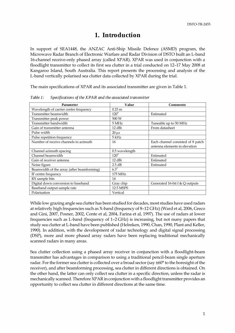
In support of SEA1448, the ANZAC Anti-Ship Missile Defence (ASMD) program, the Microwave Radar Branch of Electronic Warfare and Radar Division of DSTO built an L-band 16-channel receive-only phased array (called XPAR). XPAR was used in conjunction with a floodlight transmitter to collect its first sea clutter in a trial conducted on 12–17 May 2008 at Kangaroo Island, South Australia. This report presents the processing and analysis of the L-band vertically polarised sea clutter data collected by XPAR during the trial. The main specifications of XPAR and its associated transmitter are given in Table 1. Table 1: Specifications of the XPAR and the associated transmitter
Parameter Value Comments Wavelength of carrier centre frequency 0.23 m Transmitter beamwidth 120o Estimated Transmitter peak power 500 W Transmitter bandwidth 5 MHz Tuneable up to 50 MHz Gain of transmitter antenna 12 dBi From datasheet Pulse width 20 s Pulse repetition frequency 5 kHz Number of receive channels in azimuth 16 Each channel consisted of 8 patch
antenna elements in elevation Channel azimuth spacing 0.5 wavelength Channel beamwidth 120o Estimated Gain of receiver antenna 12 dBi Estimated Noise figure 2.5 dB Estimated Beamwidth of the array (after beamforming) 6.3o IF centre frequency 175 MHz RX sample bits 14 Digital down conversion to baseband Gray chip Generated 16-bit I & Q outputs Baseband output sample rate 12.5 MSPS Polarisation Vertical
While low grazing angle sea clutter has been studied for decades, most studies have used radars at relatively high frequencies such as X-band (frequency of 8–12 GHz) (Ward et al, 2006, Greco and Gini, 2007, Posner, 2002, Conte et al, 2004, Farina et al, 1997). The use of radars at lower frequencies such as L-band (frequency of 1–2 GHz) is increasing, but not many papers that study sea clutter at L-band have been published (Helmken, 1990, Chan, 1990, Plant and Keller, 1990). In addition, with the development of radar technology and digital signal processing (DSP), more and more phased array radars have been replacing traditional mechanically scanned radars in many areas. Sea clutter collection using a phased array receiver in conjunction with a floodlight-beam transmitter has advantages in comparison to using a traditional pencil-beam single aperture radar. For the former sea clutter is collected over a broad sector (say ±60° to the boresight of the receiver), and after beamforming processing, sea clutter in different directions is obtained. On the other hand, the latter can only collect sea clutter in a specific direction, unless the radar is mechanically scanned. Therefore XPAR in conjunction with a floodlight transmitter provides an opportunity to collect sea clutter in different directions at the same time.

DSTO-TR-2455
2
One of the key criteria for the success of phased array radars is their calibration. The calibration of XPAR data is presented in Section 2. For each dataset collection, XPAR first collected a calibration dwell, usually consisting of 20 pulses, with the transmitter turned off and transmitted pulses fed directly to the receiver. Amplitude calibration and phase calibration are carried out for the pulse uncompressed data. After pulse compression, the compressed data is further calibrated using the Wiener-Hopf filter to align outputs of the other channels with the reference channels. It was found that channels of XPAR in the data dwell have distorted noise levels, which was identified as being due to interference from the noise floor of the transmitter (the transmitter was not turned off during the receive period. A strong lesson learnt from this is that the transmitter must be turned off when receiving data). The interference is composed of a constant component and a Gaussian component. Only the constant component can be removed from the sea clutter data. A detailed interference model is presented and the estimation of the interference is discussed in detail. The interference signal can be totally removed from all channels, if channels only contain thermal noise (sea clutter-free range bins). Sea clutter processing and analysis are presented in Sections 3 and 4. The processing includes compensation of the transmit and receive azimuth patterns. In the sea clutter analysis, important properties including backscatter coefficient, spatial and temporal distributions, correlations and Doppler spectrum are analysed, with explanations for the observed phenomena.
2. Calibration of XPAR Data
Two datasets, named kix040 and kix022, have been processed and analysed in this report. Unless stated otherwise, results shown in this section and following sections are from kix040. Detailed analysis of kix022 is presented in Appendix A. When collecting each dataset, XPAR first collected a calibration dwell of 20 pulses before collecting the following data dwell. The calibration is carried out using a calibration dwell. During the calibration dwell, as shown in Figure 1, instead of feeding the transmit antenna, pulses were switched (with attenuation) to the receive feed. The received signal, after being processed and digitally down-sampled to the baseband, is then ready for calibration. During some data dwell collections, the transmitted signal was also fed to a so-called delayed transponder. The delayed transponder is a RF-to-fibre-to-RF unit with a fibre delay line equivalent to about 7 km in free space. The transmitted pulse after being delayed by the fibre line was radiated by the transponder (two L-band vertical dipoles) at front of the array as shown in Figure 2. This point source signal can be considered as a constant radar cross-section (RCS) signal for confirmation of the previous calibration. The distance between the delayed transponder and the array was 27.6 m which was largely confined by physical conditions of the test site.

DSTO-TR-2455
3
...
To TX
Calibrationdwell collection
Atennuation
Data dwellcollection
Ch 1 Ch 16
Figure 1: System calibration architecture
27.6m
Channel 16
Channel 1
Wavefront
Delayedtransponder
7.5
1 = 0.230m
Figure 2: Setup of delayed transponder and array for calibration
Subsection 2.1 discusses the details of calibration using the calibration dwell. The details of Wiener-Hopf filter are also given. Interferences from the transmitter (it was not turned off during the data collection) and their estimation and removal are discussed in Subsection 2.2. The confirmation of calibration using the delayed transponder is given in Subsection 2.3. 2.1 Calibration Using the Calibration Dwell
Calibration using the calibration dwell is composed of three steps:
1. Amplitude calibration for uncompressed signal;
2. Phase calibration for uncompressed signal; and
3. Calibration of compressed signal. 2.1.1 Amplitude Calibration for the Uncompressed Signal
Despite best efforts, the gain of each channel may be different and vary with time. During the trial a calibration dwell was collected prior to the data dwell as shown in Figure 3. The calibration dwell allows calibration to be carried out for the following data dwell. Figure 4 (a) shows amplitude profiles of individual channels for a single pulse. It can be seen that the performance of channel 7 is abnormal, and the gains of other channels differ from each other. Without loss of generality, channel 1 was selected as the reference channel, and the amplitude calibration is to multiply a constant to every other channel so that the integral of the amplitude over the pulse is equal to that of the reference channel. The resultant of amplitude calibration for uncompressed range profiles is shown in Figure 4 (b).

DSTO-TR-2455
4
Time
Calib dwell Data dwell
. . . . . .
Figure 3: Collection of the calibration dwell and data dwell in a run
50 100 150 200 250 300 3500
0.2
0.4
0.6
0.8
1
1.2
Range bin
Ampl
itude
of r
ecei
ved
sign
al
Channel 7
Other channels
50 100 150 200 250 300 350
0
0.2
0.4
0.6
0.8
1
1.2
Range bin
Ampl
itude
of r
ecei
ved
sign
al
Other channels
Channel 7
(a) (b)
Figure 4: Amplitude calibration for the uncompressed signal: (a) before amplitude calibration and (b) after amplitude calibration (note the abnormal performance of channel 7)
2.1.2 Phase Calibration for the Uncompressed Signal
Phase calibration involves two steps. The first step is to synchronise the sampling time while the second step removes the time independent phase term to align the phase of all channels. The chirp function is given by,
2
222exp)( t
T
Bt
Bjtf (1)
where B is the linear frequency modulation (LFM) bandwidth, T the pulse width and
Tt 0 the sampling time. Without loss of generality, channel 1 is defined as the reference channel with phase,
12
1 222)(
t
T
Bt
Bt Tt 0 (2)
where the term 1 accounts for relative phase of the signal and is independent of time. If there are N channels, the phase of the ith channel can be written as,
iiii ttT
Btt
Bt
2
222)( Ni ,,2 Tt 0 (3)
DSTO-TR-2455
5
where it , Ni ,,2 , denotes the time error for the ith channel which may occur in a not-well-
synchronised timing among channels (XPAR uses multiple sampling cards). The phase difference between the two is,
ii
ii tT
tBt
2)( 1 Ni ,,2 Tt 0 (4)
where
2
1 222 iiii t
T
Bt
B is independent of t .
Equation (4) indicates that by detecting the slope of the phase difference, the time error it can
be determined. However, in the implementation we assume, 0tmt ii (5)
where ,2,1,0 im and nst 100 which is the system’s ADC clock period. This is
suspected to be caused by any possible mis-synchronisation of the radar’s timing system. That is, the potential time errors between channels are multiple cycles of the ADC clock period. After im , Ni ,,2 , is determined, the digitised uncompressed range profile is resampled to
synchronise sampling time for all channels. The absolute phase difference term ii 1 ,
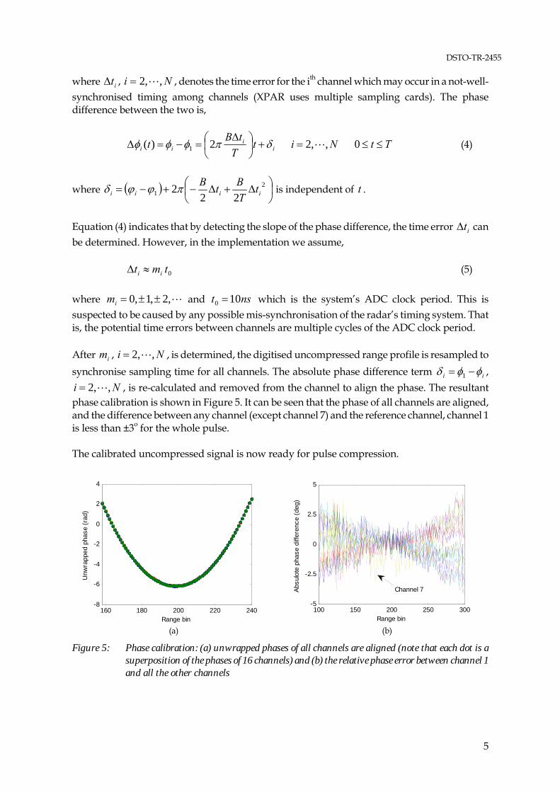
Ni ,,2 , is re-calculated and removed from the channel to align the phase. The resultant phase calibration is shown in Figure 5. It can be seen that the phase of all channels are aligned, and the difference between any channel (except channel 7) and the reference channel, channel 1 is less than ±3o for the whole pulse. The calibrated uncompressed signal is now ready for pulse compression.
160 180 200 220 240-8
-6
-4
-2
0
2
4
Range bin
Unw
rapp
ed p
hase
(rad
)
100 150 200 250 300
-5
-2.5
0
2.5
5
Range bin
Absu
lote
pha
se d
iffer
ence
(deg
)
Channel 7
(a) (b)
Figure 5: Phase calibration: (a) unwrapped phases of all channels are aligned (note that each dot is a superposition of the phases of 16 channels) and (b) the relative phase error between channel 1 and all the other channels

DSTO-TR-2455
6
2.1.3 Calibration of the Pulse Compressed Signal
After pulse compression, further calibration follows. It can be seen in Subsection 2.1.1 that although the integral of the amplitude over a pulse for all channels is equal, the amplitudes of channels for each range bin are different. Similar situation exists for the phase calibration in Subsection 2.1.2. Therefore, there is a need of further calibration after the signal is pulse compressed. The pulse-compressed range profile of a calibration pulse represents a return from a stationary point target. The desired goal of this calibration is to achieve an identical return in each channel from a calibration pulse. In the calibration, the pulse-compressed and pulse-averaged range profile of channel 1 is again used as the reference channel. Profiles of all other channels are calibrated using the Wiener-Hopf filtering technique. In the context of discrete finite-impulse-response (FIR) filtering, the Wiener-Hopf filter is also an adaptive least mean squares filter. The filter is also called Wiener filter whose details can be found elsewhere (Haykin, 2002, Chapter 2, Dong and Merrett, 2009). However for independence of this report, we repeat details of the filter here. For an input range sequence )(, kx pn , for channel n , pulse p and range bin k , the output of
the filter is,
2/)1(
2/)1(,, )()()(ˆ
M
Mmpnnpn mkxmwkx (6)
where M is the order of the filter. Equation (6) indicates that the output )(ˆ , kx pn of the filter is
estimated by a linear combination of )(, kx pn and its 1M neighbouring measurements, and
the M weights )(mwn for channel n are yet to be determined. The goal of the filter is to
minimise the mean square error (MMSE), 2
,1 |)(ˆ)(|min kxkxE pnwn
(7)
for all p and k . The sequence )(1 kx is the reference profile, i.e., pulse-averaged range profile of channel 1. The solution of (7) is not difficult to derive, which is, nn
Hn zRw 1 Nn ,,2 (8)
where )2/)1(()0()2/)1(( MwwMw nnnn w and the superscript H denotes
the Hermitian transpose.
Kk
Kkk
P
p
Hpnpnn kk
PK
0
0 1,, )()(
1
12
1xxR (9)
Kk
Kkk
P
ppnn kkx
PK
0
0 1,
*1 )()(
1
12
1xz (10)

DSTO-TR-2455
7
where the superscript * denotes complex conjugate. Note that in (10) )(*1 kx is a single element,
and )(, kpnx in (9) and (10) is a column vector, as
Tpnpnpnpn MkxkxMkxk )2/)1(()()2/)1(()( ,,,, x (11)
where the superscript T denotes transpose. In (9) and (10) 0k is the range bin that contains the
maximum value of the calibration pulse response. In this report the parameters used are 7M , 20K and 20P . After the weights were regressed, all range profiles were filtered
accordingly for channels 2 to 16 for all pulses. The range profiles of channel 1 remained unchanged. Figure 6 and Figure 7 show the effectiveness of the Wiener-Hopf filter. After filtering, it can be seen that the amplitude profile of the calibration pulse and its sidelobes for all channels (except channel 7) are almost identical, with minimal differences seen only in the sidelobe notches. Similar situation is also seen in their phase difference profiles with the notch bins having the maximum phase differences of less than 10° (except channel 7). Although channel 7 displayed abnormal performance compared to other channels, its calibrated profile is not as bad as initially thought and certainly still usable in beamforming. The zoomed-out signal range profiles with and without channel 7 are shown in Figure 8. It can be seen from Figure 8 (a) that all other 15 channels are almost identical for the mainlobe of the signal as well as its sidelobes down by 50 dB. The signal range profile of channel 7 is not as good as other channels, but still at an acceptance level as shown in Figure 8 (b). For a phased array radar, it is possible that some array element(s) may fail during operation. To minimise the beamforming distortion, weights used in the beamforming have to be updated accordingly. Two popular algorithms for finding the optimal weights, genetic algorithm (GA) and particle swarm (PS) algorithm, are introduced and discussed in Appendix B where examples of finding the optimal weights for element failure as well as for special sidelobe requirement are given.
60 65 70 75 80 85-10
0
10
20
30
40
50
Range bin
Rec
eive
d si
gnal
(dB)
Channel 7
60 65 70 75 80 85
-10
0
10
20
30
40
50
Range bin
Rec
eive
d si
gnal
(dB)
Channel 7
(a) (b)
Figure 6: Pulse compressed range profiles: (a) before Wiener-Hopf filtering and (b) after Wiener-Hopf filtering (note the profiles are the superposition of 16 channels)

DSTO-TR-2455
8
60 65 70 75 80 85-200
-100
0
100
200
Range bin
Phas
e di
ffere
nce
(deg
)
Channel 7
60 65 70 75 80 85
-40
-30
-20
-10
0
10
20
30
40
Range bin
Phas
e di
ffere
nce
(deg
)
Channel 7
(a) (b)
Figure 7: Phase difference between channel 1 and other channels for pulse compressed profiles: (a) before Wiener-Hopf filtering and (b) after Wiener-Hopf filtering
0 50 100 150-10
0
10
20
30
40
50
Range bin
Sign
al le
vel (
dB)
0 50 100 150
-10
0
10
20
30
40
50
Range bin
Sign
al le
vel (
dB)
(a) (b)
Figure 8: Signal range profiles: (a) superimposition of all channels without channel 7 (b) the profile of channel 7 (in green) is further superimposed
It is worth mentioning that due to the lower gain of channel 7, the dynamic range from the maximum signal level to the minimum noise level (thermal noise floor) is smaller than other channels. To match with other channels, the calibration processing increases the output level of channel 7 by multiplying a coefficient greater than unit. On the other hand, the dynamic range is unchangeable. As a result, the thermal noise floor of channel 7 after calibration will be higher than other channels. This is shown in Figure 9 where all channels except channel 7 have approximately the same noise level while the noise floor of channel 7 is higher than others. The relative noise floors for all 16 channels are shown in Figure 10. The noise floor is obtained by averaging all 20 calibration pulses and range bins between 500 and 2000. It can be seen that that while the noise floors of all 15 channels are at the same level with a small fluctuation of ±0.5 dB, the noise floor of channel 7 is 6.5 dB higher than the others.

DSTO-TR-2455
9
0 500 1000 1500 2000-50
-25
0
25
50
Range bin
Sign
al le
vel (
dB)
0 500 1000 1500 2000
-50
-25
0
25
50
Range bin
Sign
al le
vel (
dB) Channel 7
(a) (b)
Figure 9: Pulse compressed range profiles: (a) all channels without channel 7 (b) the profile of channel 7 is superimposed
2 4 6 8 10 12 14 16-22
-20
-18
-16
-14
-12
-10
Channel
Rel
ativ
e no
ise
leve
l (dB
)
Figure 10: Relative noise floors of all 16 channels averaged by 20 pulses and 1500 range bins
2.1.4 Absolute Power level
The average noise floor of each channel (except channel 7) shown in Figure 10 may be assumed to be equal to the thermal noise floor plus the noise figure of the channel. Its absolute value is, fn nBkTP 0100 log10 (12)
where k is the Boltzmann’s constant ( 231038.1 k Ws/K), 0T the room temperature in
Kelvin degrees ( KT 300 ), B the bandwidth of the channel (B=5 MHz) and fn the noise figure
of the channel which is estimated about 2.5 dB. This gives, dBPn 3.1345.2)1053001038.1(log10 623
100 (13)
Therefore the relative noise level of -19 dB shown in Figure 10 should be interpreted as -134.3 dB in the absolute level, that is, a constant of -115.3 dB should be added to all sea clutter range profiles shown in this report if the absolute level of sea clutter is required.
DSTO-TR-2455
10
2.1.5 Beamforming
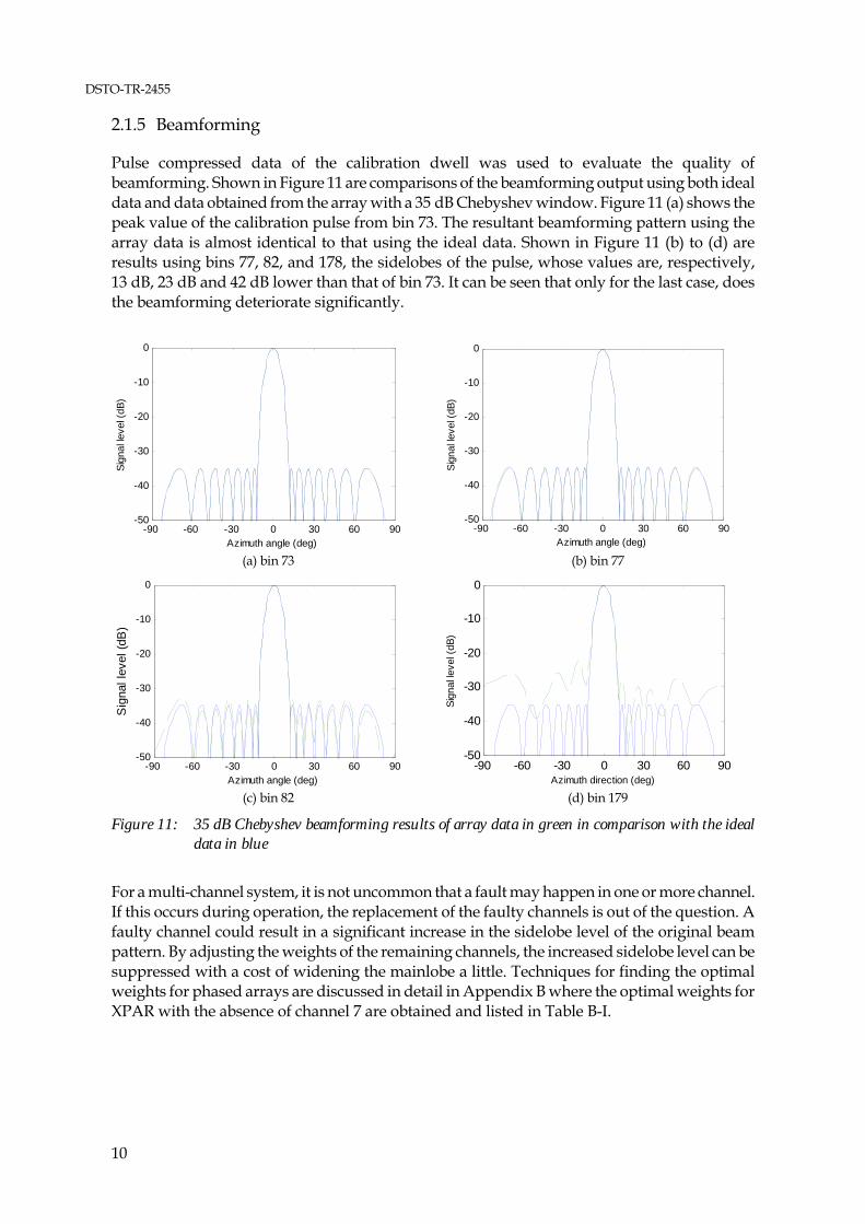
Pulse compressed data of the calibration dwell was used to evaluate the quality of beamforming. Shown in Figure 11 are comparisons of the beamforming output using both ideal data and data obtained from the array with a 35 dB Chebyshev window. Figure 11 (a) shows the peak value of the calibration pulse from bin 73. The resultant beamforming pattern using the array data is almost identical to that using the ideal data. Shown in Figure 11 (b) to (d) are results using bins 77, 82, and 178, the sidelobes of the pulse, whose values are, respectively, 13 dB, 23 dB and 42 dB lower than that of bin 73. It can be seen that only for the last case, does the beamforming deteriorate significantly.
-90 -60 -30 0 30 60 90-50
-40
-30
-20
-10
0
Azimuth angle (deg)
Sign
al le
vel (
dB)
-90 -60 -30 0 30 60 90
-50
-40
-30
-20
-10
0
Azimuth angle (deg)
Sign
al le
vel (
dB)
(a) bin 73 (b) bin 77
-90 -60 -30 0 30 60 90-50
-40
-30
-20
-10
0
Azimuth angle (deg)
Sig
nal l
evel
(dB
)
-90 -60 -30 0 30 60 90-50
-40
-30
-20
-10
0
Azimuth direction (deg)
Sign
al le
vel (
dB)
(c) bin 82 (d) bin 179
Figure 11: 35 dB Chebyshev beamforming results of array data in green in comparison with the ideal data in blue
For a multi-channel system, it is not uncommon that a fault may happen in one or more channel. If this occurs during operation, the replacement of the faulty channels is out of the question. A faulty channel could result in a significant increase in the sidelobe level of the original beam pattern. By adjusting the weights of the remaining channels, the increased sidelobe level can be suppressed with a cost of widening the mainlobe a little. Techniques for finding the optimal weights for phased arrays are discussed in detail in Appendix B where the optimal weights for XPAR with the absence of channel 7 are obtained and listed in Table B-I.

DSTO-TR-2455
11
Evaluation of beamforming with the exclusion of channel 7, using the optimal weights given in the last column of Table B-I, is shown in Figure 12. Data of the same four range bins of Figure 11 are used. It can be seen that for the first three cases, the deterioration to beam patterns is very minor, compared to the ideal pattern. Even for the last case, the degree of deterioration is much smaller compared to the last case of Figure 11, indicating that the deterioration for the last case of Figure 11 is mainly due to the data of channel 7. It can be imagined that once the hardware defect of channel 7 is fixed in the future, the calibration of the whole array can be further improved.
-90 -60 -30 0 30 60 90-25
-20
-15
-10
-5
0
Azimuth angle (deg)
Sig
nal l
evel
(dB
)
-90 -60 -30 0 30 60 90
-25
-20
-15
-10
-5
0
Azimuth angle (deg)
Sign
al le
vel (
dB)
(a) bin 73 (b) bin 77
-90 -60 -30 0 30 60 90-25
-20
-15
-10
-5
0
Azimuth angle (deg)
Sign
al le
vel (
dB)
-90 -60 -30 0 30 60 90
-25
-20
-15
-10
-5
0
Azimuth angle (deg)
Sign
al le
vel (
dB)
(c) bin 82 (d) bin 179
Figure 12: Comparison of beamforming results using array data in green and ideal data in blue. Channel 7 is excluded in beamforming and the optimal weights given in the last column of Table B-I are used in beamforming. Since channel 7 is close to the centre of the array, the minimum sidelobe level one can achieve is limited. A 20 dB sidelobe level is used in this beamforming (see Appendix B for more discussions).
This section has described the calibration of XPAR data using the calibration dwell data, and shown very satisfactory results. However, for the calibration dwell the input signal was directly injected to receiving channels and the transmitter was turned off. For the data dwell the transmitter was not switched off during the receive period, resulting in a different calibration quality for the data dwell which is examined and discussed in the following subsections.
DSTO-TR-2455
12
2.2 Interference from Transmitter and Their Removal
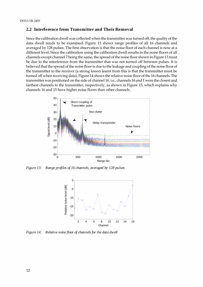
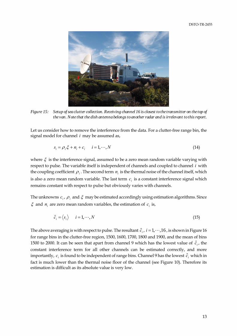
Since the calibration dwell was collected when the transmitter was turned off, the quality of the data dwell needs to be examined. Figure 13 shows range profiles of all 16 channels and averaged by 128 pulses. The first observation is that the noise floor of each channel is now at a different level. Since the calibration using the calibration dwell results in the noise floors of all channels except channel 7 being the same, the spread of the noise floor shown in Figure 13 must be due to the interference from the transmitter that was not turned off between pulses. It is believed that the spread of the noise floor is due to the leakage and coupling of the noise floor of the transmitter to the receiver (a strong lesson learnt from this is that the transmitter must be turned off when receiving data). Figure 14 shows the relative noise floor of the 16 channels. The transmitter was positioned on the side of channel 16, i.e., channels 16 and 1 were the closest and farthest channels to the transmitter, respectively, as shown in Figure 15, which explains why channels 16 and 15 have higher noise floors than other channels.
0 500 1000 1500 2000-30
-20
-10
0
10
20
30
40
50
Range bin
Sign
al le
vel (
dB)
Direct coupling of Transmitter pulse
Delay transponderNoise f loors
Sea clutter
Figure 13: Range profiles of 16 channels, averaged by 128 pulses
2 4 6 8 10 12 14 16
-20
-15
-10
-5
0
Channel
Rel
ativ
e no
ise
leve
l (dB
)
Figure 14: Relative noise floor of channels for the data dwell
DSTO-TR-2455
13
Figure 15: Setup of sea clutter collection. Receiving channel 16 is closest to the transmitter on the top of
the van. Note that the dish antenna belongs to another radar and is irrelevant to this report.
Let us consider how to remove the interference from the data. For a clutter-free range bin, the signal model for channel i may be assumed as, iiii cns Ni ,,1 (14)
where is the interference signal, assumed to be a zero mean random variable varying with respect to pulse. The variable itself is independent of channels and coupled to channel i with the coupling coefficient i . The second term in is the thermal noise of the channel itself, which
is also a zero mean random variable. The last term ic is a constant interference signal which
remains constant with respect to pulse but obviously varies with channels. The unknowns ic , i and may be estimated accordingly using estimation algorithms. Since
and in are zero mean random variables, the estimation of ic is,
ii sc ˆ Ni ,,1 (15)
The above averaging is with respect to pulse. The resultant ic , 16,,1i , is shown in Figure 16
for range bins in the clutter-free region, 1500, 1600, 1700, 1800 and 1900, and the mean of bins 1500 to 2000. It can be seen that apart from channel 9 which has the lowest value of ic , the
constant interference term for all other channels can be estimated correctly, and more importantly, ic is found to be independent of range bins. Channel 9 has the lowest ic which in
fact is much lower than the thermal noise floor of the channel (see Figure 10). Therefore its estimation is difficult as its absolute value is very low.

DSTO-TR-2455
14
2 4 6 8 10 12 14 16-60
-50
-40
-30
-20
-10
0
Channel
Sign
al le
vel (
dB)
Bin 1500Bin 1600Bin 1700Bin 1800Bin 1900Average ofBins 1500-2000
Figure 16: Constant interference signal dependent on channels but independent of range bins
Now let us estimate i . Let iii csu and note that iu is also a zero mean random variable.
Select the channel, which has the highest interference signal, i.e., the highest value of || i .
Without loss of generality, let this channel number be k , and the coupling coefficient 0|| j
kk e (i.e., zero phase reference. That is, the phase term of k is shifted to the unknown
interference , because there is no difference for finding or kje ). Since |||| kk n ,
the following initial estimates can be calculated,
2/1
2
2
||
||ˆ
k
k
u (16)
2
*
||ˆˆ
k
ki
i
uu Mi ,,1 , ki (17)
The above averaging is with respect to pulse. Since 2|| are the same for all channels, we
assume 1|| 2 , then initial values of (16) and (17) can be estimated.
The above initial estimates of i , Mi ,,1 , can be further improved by invoking correlation
properties and using a nonlinear least squares method (though Matlab’s lsqnonlin function) with a goal function of,
0Im
0Re**
**
jiji
jiji
uu
uu
Nji ,,1, and ji (18)
The estimated coupling coefficients are shown in Figure 17. It can be seen that the coupling coefficients are independent of range bins. It is interesting to note that the distribution pattern of the coupling coefficient against channel number is similar to the distribution pattern of the constant interference signal shown in Figure 16, which should not come as a surprise, because

DSTO-TR-2455
15
both the constant signal and random signal are generated by the transmitter and then coupled to the receiving channels by the same medium.
2 4 6 8 10 12 14 16-60
-50
-40
-30
-20
-10
0
Channel
| | (
dB)
Bin 1500Bin 1600Bin 1700Bin 1800Bin 1900
Figure 17: Estimated coupling coefficients
The estimate of the random interference signal which is dependent on time (pulse) and space
(range bin) can be achieved if the range bin is a clutter-free bin. The initial )(ˆ m may be estimated by,
N
ii
N
ii mu
m
1
1
)()(ˆ
Mm ,,1 (19)
where m is the pulse number. The initial estimate )(ˆ m , Mm ,,1 , is further improved again by invoking correlation properties and using a nonlinear least squares method (though Matlab’s lsqnonlin function) with a goal function of,
0Im
0Re
01||
0Im
0Re
0||
****
****
2
22
ijjijiji
ijjijiji
iii
uuuu
uuuu
u
Nji ,,1, and ji (20)
where 22 || ii n is the thermal noise floor of the channel determined by the calibration dwell
as shown in Figure 14. The above averaging is with respect to pulse for a given range bin.

DSTO-TR-2455
16
After finding the interference signals and ic and removing them from each channel, the
remaining signal component in should become mutually uncorrelated, and have a similar noise
floor to that shown in Figure 10. The actual thermal noise floors after the removal of interference signals and ic are shown in Figure 18 which is almost identical to Figure 10, indicating that
the interference signals have been successfully removed. The correlations between channels 15 and 16 are shown in Figure 191. It can be seen that the original data is highly correlated for all pulse offsets due to the constant interference signal ic .
After the removal of ic , Ni ,,1 , from each channel, the correlation is still high at the zero
pulse offset due to the random interference signal )(m , Mm ,,1 , coupled to channels. However when both interference signals are detected and removed from the data, the remaining thermal noise becomes totally uncorrelated.
2 4 6 8 10 12 14 16-22
-20
-18
-16
-14
-12
-10
Channel
Rel
ativ
e no
ise
leve
l (dB
)
Bin 1500Bin 1600Bin 1700Bin 1800Bin 1900
Figure 18: Relative noise floor after the interference signals are detected and removed
-100 -50 0 50 1000
0.2
0.4
0.6
0.8
1
No of pulse offset
Nor
mal
ised
cor
r coe
ff
-100 -50 0 50 100
0
0.2
0.4
0.6
0.8
1
No of pulse offset
Nor
mal
ised
cor
r coe
ff
(a) (b)
Figure 19: Normalised correlation between (a) 15s and 16s in red, 15u and 16u in blue, and (b) 15n
and 16n for range bin 1500
1 The cross-correlation coefficients were computed using Matlab’s function, xcorr(x, y, ‘coeff’), which returns biased coefficients (refer to Matlab for details). The calculation of unbiased coefficients is given in Subsection 4.2.
DSTO-TR-2455
17
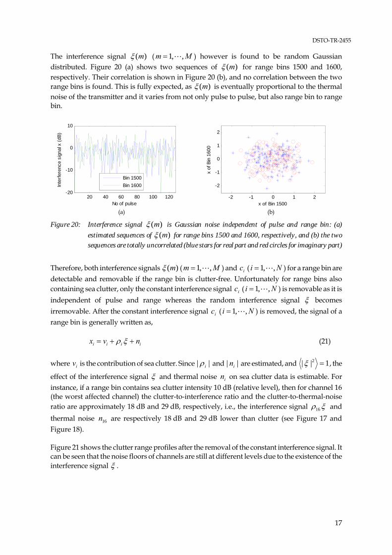
The interference signal )(m ( Mm ,,1 ) however is found to be random Gaussian distributed. Figure 20 (a) shows two sequences of )(m for range bins 1500 and 1600, respectively. Their correlation is shown in Figure 20 (b), and no correlation between the two range bins is found. This is fully expected, as )(m is eventually proportional to the thermal noise of the transmitter and it varies from not only pulse to pulse, but also range bin to range bin.
20 40 60 80 100 120-20
-10
0
10
No of pulse
Inte
rfere
nce
sign
al x
(dB)
Bin 1500Bin 1600
-2 -1 0 1 2
-2
-1
0
1
2
x of Bin 1500x
of B
in 1
600
(a) (b)
Figure 20: Interference signal )(m is Gaussian noise independent of pulse and range bin: (a) estimated sequences of )(m for range bins 1500 and 1600, respectively, and (b) the two sequences are totally uncorrelated (blue stars for real part and red circles for imaginary part)
Therefore, both interference signals )(m ( Mm ,,1 ) and ic ( Ni ,,1 ) for a range bin are
detectable and removable if the range bin is clutter-free. Unfortunately for range bins also containing sea clutter, only the constant interference signal ic ( Ni ,,1 ) is removable as it is
independent of pulse and range whereas the random interference signal becomes
irremovable. After the constant interference signal ic ( Ni ,,1 ) is removed, the signal of a
range bin is generally written as, iiii nvx (21)
where iv is the contribution of sea clutter. Since || i and || in are estimated, and 1|| 2 , the
effect of the interference signal and thermal noise in on sea clutter data is estimable. For
instance, if a range bin contains sea clutter intensity 10 dB (relative level), then for channel 16 (the worst affected channel) the clutter-to-interference ratio and the clutter-to-thermal-noise ratio are approximately 18 dB and 29 dB, respectively, i.e., the interference signal 16 and
thermal noise 16n are respectively 18 dB and 29 dB lower than clutter (see Figure 17 and
Figure 18). Figure 21 shows the clutter range profiles after the removal of the constant interference signal. It can be seen that the noise floors of channels are still at different levels due to the existence of the interference signal .

DSTO-TR-2455
18
0 500 1000 1500 2000-30
-20
-10
0
10
20
30
40
50
Range bin
Sign
al le
vel (
dB)
Direct coupling of transmitter pulse
Sea clutter
Delayed transponder
Noise f loors
Figure 21: Clutter range profiles of individual channels after the removal of the constant interference
signal and the calibration using the delayed transponder. The profiles are averaged by 128 pulses.
2.3 Confirmation Using a Delayed Transponder
As shown in Figure 2, transmitted pulses after being delayed by an optical fibre line are radiated by the transponder (two L-band vertical dipoles) at front of XPAR. Since the dipoles have a broad beamwidth, signals received by all channels can be assumed to have the same strength. The separation between the transponder and the array which was confined by conditions of the test site just marginally falls in the far field region. The phase difference caused by path lengths from the source (the transponder antenna) to the centre of the array and to the outer most channel reaches 21.1° (the far field criteria normally requires the phase difference less than 22.5°) In addition, the multi-path reflection/scattering by the ground surface is also unavoidable. If these effects are not considered to be dominant, the delayed transponder can be regarded as a stationary constant RCS target in the boresight direction and used for confirmation of beamforming. Figure 22 (a) shows a close-look of the response of a pulse from the delayed transponder. The phase differences between channel 1 and other channels are shown in Figure 22 (b). Magnitudes and phases of the mainlobe spread a few dB and a few tens degrees, respectively, amongst channels. These differences may attribute to the multi-path reflections from the path of transponder-ground-array, the direct path difference from transponder to channels, the interference from transmitter, as well as the background noise, i.e., the sea clutter. For lower sidelobes and notches where the signal level is comparable or below the level of the sea clutter (see Figure 21), both the amplitudes and phases of channels will not be identical. This is why the phase differences for the notch bins shown in Figure 22 (b) become significantly large. Results of beamformed transponder signal as a stationary constant target in the boresight direction are further shown in Figure 28 and Figure 29 in Section 3. It can be seen that the delayed transponder appears to be a good stationary target in the boresight direction.

DSTO-TR-2455
19
600 605 610 615 620 625 630-30
-20
-10
0
10
20
30
Range bin
Rel
ativ
e si
gnal
leve
l (dB
)
600 605 610 615 620 625 630-180
-135-90
-450
4590
135180
Range bin
Phas
e di
fere
nce
(deg
)
(a) (b)
Figure 22: Response of a pulse from the delayed transponder: (a) amplitude (b) phase difference between channel 1 and other channels
3. Analysis of Sea Clutter
Information of weather and the sea surface that is useful for sea clutter analysis was recorded accordingly during the trial. Weather parameters were recorded using a DSTO’s portable weather station set up next to the radar, and the data recorded by the Bureau of Meteorology’s (BOM) Weather Station at Cape Borda (about 35 km away from the test site) is also available. Sea waves were recorded by a directional wavebuoy deployed during the trial. The parameters for a dataset analysed in this report are given in Table 2. Note that the direction of the wind is defined as ‘originated from’. Another dataset is also analysed and the results are given in Appendix A. The significant wave height is the mean height of the highest one-third of the waves. The average wind speed is the wind speed averaged over every 30 minutes. The definition of gust given by BOM is that a gust is any sudden increase of wind of short duration, usually a few seconds. Table 2: Recorded weather and wave parameters
Dataset Average wind
direction wrt
North (°)
Relative to
boresight of array
(°)
Average wave
direction wrt
North (°)
Average wind speed (m/s)
Gust speed (m/s)
Temp (°C)
Significant wave height,
moH (m)
Max wave height,
maxH (m)
kix040 230 52 222 4.7 25 15.2 2.8 6.6
The boresight direction of XPAR is 178oN. Therefore, for instance, the upwind direction of kix040 is 52° relative to the boresight of XPAR as shown in Figure 23.
Ch 1 Ch 16
Boresightdirection
o178Winddirection
o230N
N
52o
Figure 23: Relative angle of the upwind direction to the boresight direction of XPAR

DSTO-TR-2455
20
This section first calculates the backscatter coefficient of sea clutter. Sea clutter intensity (power) decreasing with range and its dependence on the sea surface and weather conditions are shown. The beam azimuth pattern is corrected for beamformed sea clutter. Other popular sea clutter properties are presented in Section 4. 3.1 Backscatter Coefficient of Sea Clutter
Knowledge of the transmitter and receiver gains, peak transmit power, pulse compression ratio etc, allows the sea clutter backscattering coefficient 4
0F to be calculated using the radar
equation where F is the multipath propagation factor (Billingsley, 2002, pp. 24–25). According to the radar equation, the received power rP , after pulse compression, from a target with a RCS of at a range distance r is (Skolnik, 1990, Chapter 2, Lewis et al, 1982, Chapter 2),
Lr
FGGPP rttr 43
42
)4(
(22)
where is the pulse compression ratio ( Bt , t is the length of pulse and B is the LFM
bandwidth), tP is the transmitted power, tG and rG are the transmit and receive antenna gains,
respectively, is the radar carrier wavelength and L is the total system loss. For distributed scatterers, such as the sea surface, AFF 4
04 , where A is the area of the range cell, and
sec2B
crA for the pulse limited (range limited) case with range compression, is the
radar’s azimuth beamwidth, the grazing angle ( 1sec for low grazing angles) and c the speed of light. Finally we have,
3103
2
104
0 log102)4(
log10)( rB
c
L
GGPdBPF rtt
r
2 2dBm m (23)
Parameters of (23) may be found in Table 1. In addition the system loss L was estimated to be 3 dB. Since the height the radar relevant to the sea levels is known (61 m), the grazing angle corresponding to range can be calculated using the classical 4/3 Earth radius model (Long, 2001, Chapter 2). Note that the received power )(dBPr in (23) is the absolute level as discussed in Subsection 2.1.4, but not the relative level shown in Figure 21. The sea clutter backscatter coefficient against grazing angle for sea clutter dominant bins calculated by (23) is shown in Figure 24 which is in good agreement with values of 4
0F published in radar handbooks
(Nathanson, 1999, Chapter 7, Long, 2001, Chapter 6). For instance, according to Nathanson (1999, Chapter 7), typical 4
0F values of the L-band vertically polarised sea clutter at grazing
angle of 1° are −54 dB and −45 dB for sea states of 3 and 4, respectively. The sea states of the two datasets kix040 and kix022 used in this report are about 4 and 3 according to their wind and wave conditions which are given in Table 2 and Table A-I, respectively.

DSTO-TR-2455
21
0.8 1 1.2 1.4-60
-55
-50
-45
-40
Grazing angle (deg)
0 F
4 (dB)
Dataset A
Dataset B
Figure 24: Calculated sea clutter coefficient against grazing angle using (23) averaged by 16 channels
and 512 pulses. Blue and red curves are for datasets kix040 and kix022, respectively (details of kix022 can be found in Appendix A).
3.2 Decrease of Sea Clutter Intensity (Power) against Range
Figure 25 shows azimuth-range maps for range bins 250–750 after data is beamformed using a single pulse. In particular Figure 25 (a) is the result of a uniform beamforming processing window. As a result the response of the delayed transponder in range bin 615 is composed of not only a mainlobe at the zero degree azimuth (boresight of XPAR) but also sidelobes spreading over the whole azimuth. The sidelobes can be greatly depressed if a 35 dB Chebyshev window is applied as shown in Figure 25 (b). The response appears in range bin 579 at -39° azimuth (relative to the boresight of receive) is from an unknown target. Although the Chebyshev window suppresses the sidelobes, it also introduces distortions, broadens the mainlobe and reduces the azimuth resolution. The sea clutter analysis in this report uses a uniform window.
(a) Uniform window (b) 35dB Chebyshev window
Figure 25: Azimuth-range clutter maps resulted from (a) a uniform window and (b) a 35 dB Chebyshev window for range bins 250–750
Kix040
Kix022
DSTO-TR-2455
22
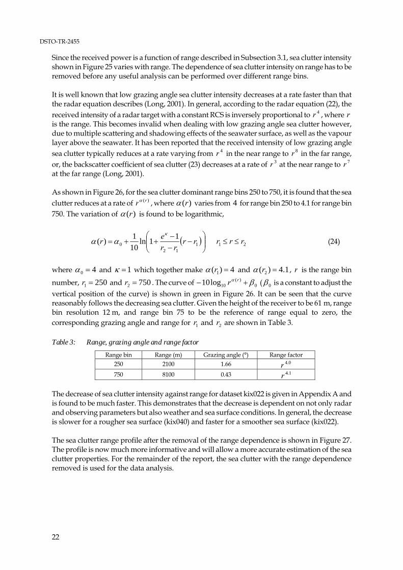
Since the received power is a function of range described in Subsection 3.1, sea clutter intensity shown in Figure 25 varies with range. The dependence of sea clutter intensity on range has to be removed before any useful analysis can be performed over different range bins. It is well known that low grazing angle sea clutter intensity decreases at a rate faster than that the radar equation describes (Long, 2001). In general, according to the radar equation (22), the received intensity of a radar target with a constant RCS is inversely proportional to 4r , where r is the range. This becomes invalid when dealing with low grazing angle sea clutter however, due to multiple scattering and shadowing effects of the seawater surface, as well as the vapour layer above the seawater. It has been reported that the received intensity of low grazing angle sea clutter typically reduces at a rate varying from 4r in the near range to 8r in the far range, or, the backscatter coefficient of sea clutter (23) decreases at a rate of 3r at the near range to 7r at the far range (Long, 2001). As shown in Figure 26, for the sea clutter dominant range bins 250 to 750, it is found that the sea clutter reduces at a rate of )(rr , where )(r varies from 4 for range bin 250 to 4.1 for range bin 750. The variation of )(r is found to be logarithmic,
112
0
11ln
10
1)( rr
rr
er
21 rrr (24)
where 40 and 1 which together make 4)( 1 r and 1.4)( 2 r , r is the range bin
number, 2501 r and 7502 r . The curve of 0)(
10log10 rr ( 0 is a constant to adjust the
vertical position of the curve) is shown in green in Figure 26. It can be seen that the curve reasonably follows the decreasing sea clutter. Given the height of the receiver to be 61 m, range bin resolution 12 m, and range bin 75 to be the reference of range equal to zero, the corresponding grazing angle and range for 1r and 2r are shown in Table 3. Table 3: Range, grazing angle and range factor
Range bin Range (m) Grazing angle (°) Range factor
250 2100 1.66 0.4r 750 8100 0.43 1.4r
The decrease of sea clutter intensity against range for dataset kix022 is given in Appendix A and is found to be much faster. This demonstrates that the decrease is dependent on not only radar and observing parameters but also weather and sea surface conditions. In general, the decrease is slower for a rougher sea surface (kix040) and faster for a smoother sea surface (kix022). The sea clutter range profile after the removal of the range dependence is shown in Figure 27. The profile is now much more informative and will allow a more accurate estimation of the sea clutter properties. For the remainder of the report, the sea clutter with the range dependence removed is used for the data analysis.

DSTO-TR-2455
23
0 200 400 600 800 1000 1200-20
-10
0
10
20
30
Range bin
Sign
al le
vel (
dB)
Figure 26: Sea clutter range profile averaged over 512 pulses and 16 channels in blue. The green curve
is the empirical curve of 0)(
10log10 rr .
250 350 450 550 650 750-40
-20
0
20
40
Range bin
Sign
al le
ve (d
B)
Figure 27: Sea clutter range profiles of 16 channels after the removal of the range dependence
A sea clutter channel-range map is shown in Figure 28 (a), where each channel’s measurement may be viewed as the data received by a radar with a broad beamwidth as wide as 120°. The azimuth-range map after beamforming is shown in Figure 28 (b). The 3D plots of azimuth-range sea clutter are shown in Figure 29. It can be seen that the behaviour of sea clutter after the removal of the range dependence is much easier to observe compared to Figure 25. In general the sea clutter azimuth-range map shows a random pattern in both the azimuth and range directions, consistent with random scattering from a rough sea surface.

DSTO-TR-2455
24
(a) sea clutter received by individual channels (b) beamformed sea clutter
Figure 28: Sea clutter (a) channel-range map before beamforming and (b) azimuth-range map after beamforming.
(a) Uniform window (b) 35dB Chebyshev window
Figure 29: 3D azimuth-range sea clutter obtained by the use of (a) a uniform window and (b) a 35 dB Chebyshev window
3.3 Beam Azimuth Pattern Correction
The beam azimuth pattern of both the transmit antenna and receive channels may be approximated as cos , oo 6060 , where is the azimuth angle relative to the boresight direction of the receiving array. Sea clutter beyond ±60° in azimuth suffers a rapid gain loss, and should not be used for detailed study. The beamformed sea clutter therefore needs a further correction to remove the effect of the beam azimuth pattern. Azimuth variations of sea clutter in range bins 300–550 before the correction are plotted in Figure 30 (a), in which the mean clutter for range bins 300–550 is also shown. The curve is generally a reflection of azimuth beam pattern of transmitter and receiver (i.e., 2cos ). The beam pattern drops approximately 3 dB at the azimuth angle ±60° for a transmitter or receiver having a cosine beam pattern. Therefore, there is approximately a 6 dB drop in sea clutter at ±60°. After the beam pattern correction (compensation), the variation of the clutter and its azimuth mean in the region of -60° to +60° is shown in Figure 30 (b). Details of the variation of the azimuth mean against azimuth angle, is further shown in Figure 31 in which the upwind and crosswind directions are also marked. According to other studies (Crisp, et al, 2006), the sea clutter azimuth pattern has the highest peak in the upwind direction, and troughs in the crosswind directions. Judging from the figure,

DSTO-TR-2455
25
it seems that a possible offset between the wind direction at the radar site (61 m above the sea surface and a few kilometres away from the spot the radar was measuring) and the wind direction on the sea was somehow about 20–30 degrees, that is, the actual upwind direction according to Figure 31 is about 200° if the sea clutter is assumed to have its peak in the upwind direction. Also the difference between the peak in the upwind direction and the trough in the crosswind direction is about 6–7 dB.
-90 -60 -30 0 30 60 90-30
-20
-10
0
10
20
30
Azimuth angle (deg)
Sign
al le
vel (
dB)
-60 -40 -20 0 20 40 60
-30
-20
-10
0
10
20
30
Azimuth angle (deg)
Sign
al le
vel (
dB)
(a) before beam pattern removed (b) after beam pattern removed
Figure 30: Sea clutter azimuthal distributions of range bins 300 to 550, as well as their mean azimuth distribution in thick blue curve
-60 -40 -20 0 20 40 607
8
9
10
11
12
13
14
15
Azimuth angle (deg)
Rel
ativ
e m
ean
clut
ter (
dB)
Upwinddirection
Crosswinddirection
Figure 31: Variation of sea clutter against azimuth (relative value, averaged over range bins 300–550)

DSTO-TR-2455
26
4. Distributions and Correlations
Figure 32 shows two sea clutter azimuth profiles for range bins 300 and 302, respectively2 received by 10 consecutive pulses. One can readily see two facts: (1) there is little correlation between the two range bins indicating that dominant scatterers in these two range bins are located at different azimuths and (2) the data of the same range bin and collected by 10 consecutive pulses are highly correlated with small differences between pulses. Spatial (range and azimuth) and temporal (pulse) distributions and correlations as well as Doppler spectral distributions are important properties which characterise sea clutter, and directly determines radar performance when detecting targets embedded in it. This section studies these properties of the sea clutter received by XPAR. However, there are limitations to the analysis of temporal correlation and Doppler spectrum using the current XPAR data. While the number of pulses used in the analysis was 512, the duration of the corresponding data collection time was relatively short (about 0.1 s), as XPAR’s pulse repetition frequency (PRF) was 5 kHz. As a consequence, correlation time longer than 0.1s becomes unmeasurable. Likewise, the resulted Doppler frequency resolution is 9.8 Hz, so slowly-varying events might not be observed accurately and the events with close Doppler frequencies become inseparable.
-60 -40 -20 0 20 40 60-20
-10
0
10
20
30
Azimuth angle (deg)
Rel
ativ
e se
a cl
utte
r int
ensi
ty (d
B)
Figure 32: Sea clutter azimuth profiles of range bins 300 (in blue) and 302 (in red) collected by 10
consecutive pulses
4.1 Spatial (Range) Probability Distribution
It is well known sea clutter spatial distribution is a function of many parameters including sea surface roughness (which in turn, is a function of meteorological parameters), radar frequency and radar illumination geometry, as well as radar resolution (Ward et al, 2006, Chapter 2). Sea clutter is also spikier at low grazing angle due to multi-path scattering and the shadowing effect.
2 The radar’s range resolution is 30m and the range bin interval is 12m, so the data of immediate range bins are not independent samples.

DSTO-TR-2455
27
One interesting point we want to discuss here is the probability distribution of the beamformed sea clutter data collected using a multi-channel receiver with a broad-beam floodlight transmitter (such as the XPAR system). The distribution appears to be less spiky than the distribution of sea clutter collected using a traditional (single aperture) narrow-beam transmit and narrow-beam receive radar system, supposing that both receivers have the same beam pattern. The difference lies in different beam patterns of transmitters as sketched in Figure 33 where the beamformed receiver beam pattern of the multi-channel receiver is assumed to be the same as that of the traditional single-aperture receiver. Different transmit beam patterns determine different levels of the sidelobe clutter entering into the radar due to different illumination levels although the receiver beam patterns are identical. Sidelobe clutter enters the radar with a higher level when using a broad-beam transmitter whereas sidelobe clutter enters the radar with a lower level when using a narrow-beam transmitter. For each range bin, the radar measurement is the vector summation of echoes entered into the mainlobe and sidelobes. As a result, the sea clutter is expected to be less spiky for the case of broad-beam transmitting, since there is more averaging in the summation of the mainlobe vector (sum of backscatter in the mainlobe) and the sidelobe vector (sum of backscatter in sidelobes).
Rx gain patternTx gain pattern
Rx gain patternTx gain pattern
(a) broad-beam transmitter and narrow-beam receiver (b) narrow-beam transmitter and narrow-beam receiver
Figure 33: Sidelobe clutter enters into radar at (a) a high level and (b) a low level due to different illumination by transmitters.
While sea clutter is less spiky when using a broad-beam transmitter (a good thing for target detection), target signals are also spreading/smearing in the azimuth (a bad thing for target detection). Consider a target present in a sidelobe position. Its signal enters into radar from the sidelobe at a high level because of high illumination of broad-beam transmitter, resulting in signal spreading/smearing in azimuth. Extending the above discussion, if a receiver beam pattern is also a broad-beam pattern, such as with XPAR before beamforming, the sea clutter is even less spiky, as scatterers in the sidelobe positions of the beamformed receiver are now in the mainlobe position of the broad-beam receiver, resulting in a further averaging through the summation. Obviously the azimuth resolution of the broad-beam receiver is very coarse. For XPAR, the azimuth resolution is 120° (i.e., ±60° relative to the boresight direction) before beamforming or 6.3° (Wirth, 2001) after beamforming. With the understanding of differences in the spatial distribution of sea clutter before and after beamforming, we now examine the spatial distribution of sea clutter collected by XPAR. The distribution is assumed to be K-distributed. The single-look K-distribution is given by (Ward et al, 2006, p. 109),

DSTO-TR-2455
28
/2)(
2)( 1
2/)1(
vzKvz
v
vzp v
v
(25)
where 2|| xz is the sea clutter intensity, zE , is the gamma function, 1vK is the
modified Bessel function of the second kind with the order of 1v and v is the shape parameter. The popularly used moment method (Blacknell, 1994) was utilised in estimating the shape parameter. It can been shown that the mean of single-look K-distributed sea clutter samples in the log domain is (Blacknell, 1994), 1ˆlnˆlnln 00 vvzz (26)
where 0 is the polygamma function of zero order and v is the estimate of the shape parameter. Listed in Table 4 are estimated values of the K-distributed shape parameter for sea clutter in range bins 300–550. The estimated shape parameter value for the data before beamforming (i.e., azimuth resolution of 120°) is 7.6. The estimated shape parameter values are 4.2 and 2.7 for beamformed (i.e., azimuth resolution of 6.3°) data in the azimuthal regions of -10° to +10° and -60° to +60°, respectively. The data before beamforming has a broad azimuthal resolution of 120°, so its distribution approaches Rayleigh and hence has a higher shape value. For the beamformed data, the mean varies with azimuth as shown in Figure 31. A wider azimuth region has a larger variation in mean (see Figure 31), resulting in a smaller estimated shape parameter (spikier) for the region. The specific shape values however, are dependent on many parameters, such as radar frequency, polarisation, grazing angle, as well as sea surface conditions and weather conditions. Figure 34 shows the estimated probability density function (pdf) of the normalised sea clutter intensity before beamforming and the associated K-distribution fit. The estimated pdfs of the beamformed sea clutter intensity are also well fitted by the K-distribution (with different shape parameters) and therefore are not shown in the report. Table 4: Estimated shape parameter values for sea clutter data in range bins 300–550 before and after
beamforming processing
Sea clutter data Shape parameter (K-distribution fit) Before beamforming (i.e., azimuth resolution of 120°) 7.6 Beamformed (i.e., azimuth resolution of 6.3°) clutter in the azimuth region of -10° to +10°
4.2
Beamformed (i.e., azimuth resolution of 6.3°) clutter in the azimuth region of -60° to +60°
2.7

DSTO-TR-2455
29
-40 -30 -20 -10 0 10 200
0.02
0.04
0.06
0.08
Normalised sea clutter intensity (dB)
-70 -60 -50 -40 -30 -20 -10 0 10 20
10-6
10-4
10-2
100
Normalised sea clutter intensity (dB)
pdf o
n lo
g sc
ale
(a) pdf on log scale (b) pdf on linear scale
Figure 34: The estimated pdf of the normalised sea clutter intensity in green dots and the K-distribution fit in blue curves: (a) pdf on linear scale to view the global fit and (b) pdf on log scale to view the tail fit
The variation of the shape parameter for beamformed sea clutter against radar azimuth is given in Table 5. The shape parameter is found to vary with the wind direction. Its trough (spikiest sea clutter) is in the crosswind direction and the peak (least spiky sea clutter) in the upwind direction. This is consistent with the features of the high grazing angle X-band sea clutter found by Crisp and his colleagues (2009). Studying sea clutter distribution in 360o azimuth collected by an airborne radar operated in the spotlight mode, Crisp and his colleagues (2009) found that the shape parameter has a sinusoidal variation in azimuth aligning with the wind direction and has its troughs in the crosswind directions and peaks in upwind and downwind directions. The spikiest sea clutter was previously found to be aligned with the swell direction (Ward, et al, 2006, page 26). Table 5: Shape parameter against azimuth direction (the upwind direction is 52°)
Azimuth -50°≤≤-30° -30°≤≤-10° -10°≤≤10° 10°≤≤30° 30°≤≤50° -60°≤≤60° Shape
parameter 1.52 3.34 4.17 6.30 7.57 2.68
4.2 Spatial Correlation
The autocorrelation coefficient is defined as,
2
*
|)(|
)()()(
txE
txtxE (27)
However in numerical calculation, the determination of the expectation may be an issue. The auto-correlation coefficient is calculated using the Matlab function, xcorr(x, ‘unbiased’)3, which is then normalised so that 1)0( . The explicit mathematical expression for the correlation coefficient used in this report is,
3 The Matlab function xcorr(x, ‘coeff’) returns biased correlation coefficients. The Matlab function xcov(x, ‘coeff’), returns biased correlation coefficients for )( xx .

DSTO-TR-2455
30
1
0
*
11
0
2
)()()(
|)(|1
)(kM
m
M
mmxkmx
kM
mxM
k 0k (28)
where k is the lagged number (e.g., range bins for spatial correlation or pulses for temporal correlation) and x is the complex sea clutter data. Note that with this definition, it is possible that 1)0(|)(| k for 0k , if (a) M is not large enough and/or (b) the sequence )(mx ,
1,,0 Mm is a non-stationary sequence. For instance, a sequence }1,2,3,4,3,2,1{ results in 1)0(06.1)1( . If, however, the sequence repeats a few times, say, 4, it results in
96.0)1( . Since XPAR’s PRF is high (5 kHz), clutter variation with respect to pulses appears ‘slow’. Using a total of 512 pulses (≈0.1 s) to calculate the temporal correlation using (28), we sometimes notice 1|)(| k for 0k , which may be interpreted as the number of samples not being large enough for the slowly varying data. The correlation calculation can be applied to a number of different measures, such as the amplitude, intensity and complex value (in-phase and quadrature data). Using different measures usually results in different correlation coefficients. For instance, a complex variable with constant amplitude and random phase would produce 0)0( k (fully uncorrelated) and 1)0( k (fully correlated) for complex and amplitude measures, respectively. There is also no need to subtract the mean before calculating the correlation unless there are reasons to do so. For instance, if the radar measures a stationary target, the measurement would be a constant signal plus zero mean thermal noise. If the mean is subtracted before calculating the correlation, the resultant correlation is measuring the noise instead of the desired target signal. 4.2.1 Spatial Correlation in Range
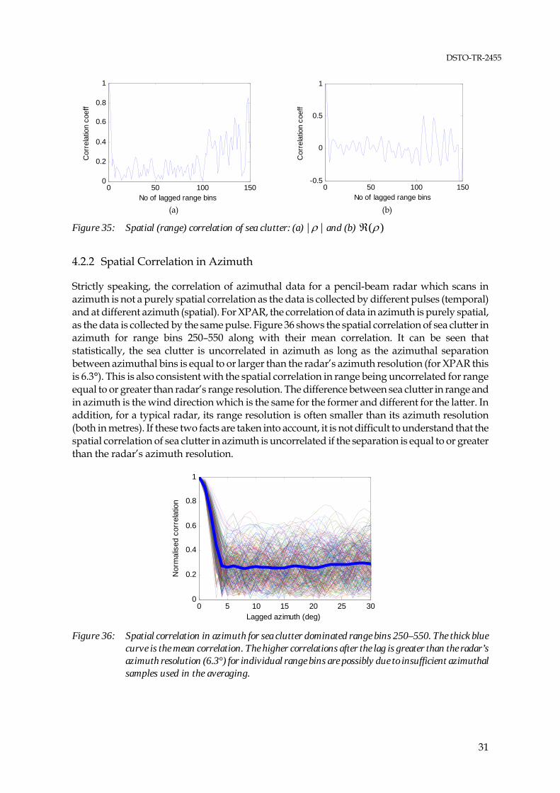
With a 5 MHz bandwidth, XPAR has a range resolution of 30 m. The actual sampling rate is 12.5 MHz, resulting in a 12 m range sampling interval causing consecutive range samples to be correlated due to over sampling. The normalised spatial correlation of range bins 250 to 400 at the azimuth 0° is shown in Figure 35 where both the absolute value and real part of the correlation coefficient, || and )( are shown. The estimated correlation coefficient indicates that the range bins whose interval is greater than 3 (greater than the radar range resolution) in general can be considered as uncorrelated as their correlation coefficient is below e/1 4. The correlation coefficient, though it is small, does not show a monotonically decreasing pattern but rather contains some features, revealing the structure of waves/swells in range (Dong 2007). The detailed analysis is difficult as the sea clutter in range is not wide-sense stationary for limited range observations, and the correlation shown in the figure is dependent on not only the time of the observation, but also the number of samples used in the averaging processing. The more the samples are used in the correlation calculation, the less oscillation of the tail. For instance, the higher correlation coefficient values for large lags shown in Figure 35 are possibly due to fewer samples used in the calculation.
4 This criterion is usually for a non-periodic correlation whose tail does not contain much information; the tail of spatial correlation of sea clutter reveals structures of waves and swells in range.
DSTO-TR-2455
31
0 50 100 1500
0.2
0.4
0.6
0.8
1
No of lagged range bins
Cor
rela
tion
coef
f
0 50 100 150
-0.5
0
0.5
1
No of lagged range bins
Cor
rela
tion
coef
f
(a) (b)
Figure 35: Spatial (range) correlation of sea clutter: (a) || and (b) )(
4.2.2 Spatial Correlation in Azimuth
Strictly speaking, the correlation of azimuthal data for a pencil-beam radar which scans in azimuth is not a purely spatial correlation as the data is collected by different pulses (temporal) and at different azimuth (spatial). For XPAR, the correlation of data in azimuth is purely spatial, as the data is collected by the same pulse. Figure 36 shows the spatial correlation of sea clutter in azimuth for range bins 250–550 along with their mean correlation. It can be seen that statistically, the sea clutter is uncorrelated in azimuth as long as the azimuthal separation between azimuthal bins is equal to or larger than the radar’s azimuth resolution (for XPAR this is 6.3°). This is also consistent with the spatial correlation in range being uncorrelated for range equal to or greater than radar’s range resolution. The difference between sea clutter in range and in azimuth is the wind direction which is the same for the former and different for the latter. In addition, for a typical radar, its range resolution is often smaller than its azimuth resolution (both in metres). If these two facts are taken into account, it is not difficult to understand that the spatial correlation of sea clutter in azimuth is uncorrelated if the separation is equal to or greater than the radar’s azimuth resolution.
0 5 10 15 20 25 300
0.2
0.4
0.6
0.8
1
Lagged azimuth (deg)
Nor
mal
ised
cor
rela
tion
Figure 36: Spatial correlation in azimuth for sea clutter dominated range bins 250–550. The thick blue
curve is the mean correlation. The higher correlations after the lag is greater than the radar’s azimuth resolution (6.3°) for individual range bins are possibly due to insufficient azimuthal samples used in the averaging.

DSTO-TR-2455
32
4.3 Temporal Correlation
The temporal correlation time is defined as the time taken for the temporal correlation coefficient to drop from 1 to 1/e. Figure 37 shows two azimuth-range maps of the temporal correlation time in milliseconds calculated by use of || and )( , respectively. For Figure 37 (a), while most pixels have a correlation time around 20 ms, a significant portion of pixels have much longer correlation times. Since the number of pulses used in the calculation is 512, the maximum correlation time shown in the figure is about 100 ms, including the correlation time for stationary targets such as the delayed transponder and the unknown target. The correlation time calculated by use of )( is generally much shorter, with the majority around 10 ms. Shown in Figure 38 are two histograms of the correlation time for sea clutter in range bins 250–500 at azimuth -60° to +60° calculated by || and )( , respectively. The last bar in the figure should be understood as the sum of the bars whose correlation time is equal to and greater than 100 ms (due to the limited temporal samples, correlation time greater than 100 ms becomes indiscriminative). On the other hand, the first bar in the figure indicates zero correlation time. It is possible that some sea clutter bins such as those containing only shadowed area, which are thermal noise only, are temporally uncorrelated.
Azimuth angle (deg)
Ran
ge b
in
-60 -40 -20 0 20 40 60250
350
450
550
650
750
0
10
20
30
40
50
60
70
80
90
100
Azimuth angle (deg)
Ran
ge b
in
-60 -40 -20 0 20 40 60250
350
450
550
650
750
0
10
20
30
40
50
60
70
80
90
100
(a) calculated by use of ρ| | (b) calculated by use of ρ( )
Figure 37: Range-azimuth maps of the temporal correlation time in milliseconds calculated by (a) || and (b) )( . The upwind direction is at azimuth 52° relative to the boresight of XPAR.
0 20 40 60 80 1000
0.01
0.02
0.03
0.04
0.05
Correlation time (ms)
0 10 20 30 40 50 60 70 80 90 100
0
0.03
0.06
0.09
Correlation time (ms)
(a) calculated by use of ρ| | (b) calculated by use of ρ( )
Figure 38: Histogram of the correlation time for sea clutter in range bins 250–550 at azimuth of -60° to +60°. The peak of the distribution is about (a) 20 ms and (b) 10 ms.

DSTO-TR-2455
33
The differences shown in Figure 37 (or Figure 38) warrant an explanation. Let us take a look at an example. Figure 39 (a) plots the variation with pulse for sea clutter in range bin 375 at 0° azimuth, and the associated correlation coefficients are shown in Figure 39 (b). The correlation coefficient || drops first below 1/e when the number of lagged pulses is 104, resulting in a correlation time of >20.8 ms. On the other hand, the correlation coefficient )( drops first below 1/e when the number of lagged pulses is 44, giving a correlation time of 8.8 ms. Since
)cos(||)( , where is the phase of , it is understood that in general )( drops
faster than || . This is why Figure 37 (or Figure 38) shows different properties of correlation time of the range-azimuth sea clutter. It also should be pointed out that since the correlation coefficient shown in Figure 39 (b) (either || or )( ) does not attenuate to zero after dropping below 1/e, but oscillates, the data cannot be said to be uncorrelated even though the data’s separation is much larger than the correlation length. Therefore, the correlation time shown in Figure 37 and Figure 38 is only indicative, since after the correlation time, the data does not necessarily become uncorrelated, as shown in Figure 39. One can also see that Figure 37 (b) clearly shows that statistically the correlation time of sea clutter in the upwind direction is much longer than that in other directions. This is due to the radar seeing more sea spikes (higher returns) in the upwind direction, and the correlation time of sea spikes is usually much longer than the other components, such as capillary waves (Ward, et al, 2006, Chapter 2).
0 128 256 384 512-30
-20
-10
0
10
20
30
Pulse
Sign
al le
vel (
dB)
0 100 200 300 400 500
-1
-0.5
0
0.5
1
No of lagged pulses
Cor
rela
tion
coef
f
(a) (b)
Figure 39: (a) Sea clutter variation with pulse and (b) the corresponding correlation coefficients calculated by || in green and )( in blue. The dashed red line is the threshold of 1/e.
4.4 Temporal Probability Distribution
A total of 512 temporal (pulse) samples for each range-azimuth bin are used to estimate the temporal probability distribution. However the number of the equivalent independent and identically distributed (iid) samples for each range-azimuth bin is much smaller due to correlation which would result in an inaccurate estimation (Dong and Crisp, 2009). In order to have an accurate estimation, more samples are needed. Suppose that all range-azimuth bins have an identical temporal distribution, we normalise data samples in each range-azimuth bin with respect to pulses, and then use all the samples from different range-azimuth bins to estimate the pdf. Figure 40 shows the estimated pdf of the normalised temporal range-azimuth sea clutter intensity collected by 512 pulses for range bins 250–550 and azimuthal region of -60° to +60°. It is seen that the distribution has a narrower shape than the exponential distribution, a distribution for intensity of Rayleigh distributed data.

DSTO-TR-2455
34
In general, the temporal distribution of sea clutter is expected to be Rayleigh according to the well known two-component K-distributed sea clutter model (Ward et al, 2006), in which the K-distributed clutter is composed of a fast-varying Rayleigh component (due to variation of speckle) modulated by a slow-varying gamma component (due to variation of underlying mean). Since the variation of underlying mean is slow (on the order of seconds to tens of seconds), during the observation period (0.1 s), the underlying mean can be assumed unchanged. The temporal distribution of sea clutter intensity difference from the exponential distribution needs an explanation. While there are as many as 512 temporal samples in each range-azimuth bin, the number of equivalent iid samples in each range-azimuth bin is rather small because of the temporal correlation. As a result, the mean of each range-azimuth bin cannot be estimated correctly since the data in each a range bin tends to have similar values rather than random values. After the normalisation by each bin’s mean, higher measurements (relative to its ‘true’ mean) will then become lower and vice versa, resulting in a narrower distribution in a short sampling duration. To verify this, a dataset consisting of 10,000 range bins was simulated. Each range bin contains 512 temporal samples collected at a PRF of 5000 Hz. These 512 samples are assumed to be Gaussian and have exponential correlation with a correlation time of 20 ms which is expressed by the spherically invariant random process (SIRP) (Rangaswamy et at, 1993, Antipov, 1998). After each range bin was normalised by its mean with respect to pulse, the pdf of 10,000 × 512 samples is shown in Figure 41. It can be seen that the distribution of the simulated data is very similar to the temporal distribution of sea clutter shown in Figure 40. Dataset kix022 has almost the same temporal distribution as dataset kix040.
-30 -15 0 150
0.02
0.04
0.06
0.08
0.1
0.12
Clutter intensity (dB)
-60 -45 -30 -15 0 15
10-6
10-4
10-2
100
Clutter intensity (dB)
Pdf o
n lo
g sc
ale
(a) (b)
Figure 40: Temporal distribution of sea clutter in range-azimuth bins, the data’s pdf in blue line-circle compared with the exponential distribution in green line. The pdfs are plotted on (a) linear scale to view the global distribution and (b) log scale to view the tails’ distribution.

DSTO-TR-2455
35
-30 -20 -10 0 100
0.02
0.04
0.06
0.08
0.1
0.12
Intensity (dB)
-60 -45 -30 -15 0 1510
-6
10-4
10-2
100
Intensity (dB)
Pdf o
n lo
g sc
ale
(a) Pdf on linear scale (b) Pdf on log scale
Figure 41: Shown in blue line-circle is the histogram of simulated data composed of 10,000 range bins. Each range bin has 512 temporal Gaussian samples sampled with a PRF of 5000 Hz and has an exponential correlation with a correlation time of 20 ms. Data in each range bin is normalised by its mean. The green curve is the pdf of an exponential distribution.
Based on the above analysis, we can conclude that the temporal distribution of sea clutter intensity/amplitude collected by the XPAR is exponential/Rayleigh distributed. Due to the short observation time, the mean of clutter intensity in each bin cannot be estimated accurately, and the resultant distribution appears to be narrower than the exponential distribution. The temporal distribution of sea clutter is therefore dependent on the observation time. If the observation time is in the order (or a few times) of the correlation time, the intensity distribution will be narrower than exponential as the mean of the data cannot be estimated accurately. It is understandable, for a slowly-varying Gaussian signal, fast sampling in a short period would result in almost identical samples (Dirac delta function like). The distribution will become exponential if the observation time is tens to hundreds of the correlation time and the mean can be estimated accurately. For a very long observing period, say, more than tens of seconds to minutes, the data will become the K-distributed as the underlying mean of sea clutter has varied due to the propagation of waves. 4.5 Doppler Spectra of Sea Clutter
The Doppler spectrum of sea clutter is a combination of radar parameters (frequency, polarisation and illumination geometry etc) and environmental parameters (such as directions and scales of wind and swell). Broadly speaking, therefore, the Doppler spectrum of sea clutter is not time stationary due to fluctuations in the environment over time. The Doppler spectrum (power spectrum density (PSD) in dB) map for sea clutter in range bins 250–750 at 0° azimuth (boresight of XPAR), calculated by 512 pulses is shown in Figure 42. It can be seen that the Doppler frequency of the delayed transponder (a stationary target) is centralised at zero Hertz. The peak of the Doppler frequency for sea clutter dominant bins is in the region 10–20 Hz, indicating that sea clutter was moving towards the radar. The PRF of the radar is 5000 Hz, so the unambiguous frequency band is -2500 Hz to 2500 Hz, and the figure only shows a portion of the frequency band to emphasise details of sea clutter’s Doppler spectra. The Doppler analysis and the temporal correlation analysis are cousin analyses and one in the frequency domain and the other in the time domain. For the temporal correlation

DSTO-TR-2455
36
analysis, it has been shown that the sampling period (about 0.1 s) was not long enough. The same issue exists in the Doppler analysis as the Doppler resolution, 5000/512 = 9.8 Hz, is relatively coarse for spectrum of sea clutter. On the other hand, a high PRF allows a large sea clutter free unambiguous Doppler spectral band which is advantageous in detecting targets with high velocities.
Frequency (Hz)
rang
e bi
n
-100 -75 -50 -25 0 25 50 75 100250
350
450
550
650
750
10
20
30
40
50
60
70
80
90
100
Figure 42: Doppler spectrum (in dB) of sea clutter in range bins 250–750 at 0° azimuth (boresight of
XPAR)
Figure 43 shows the Doppler spectrum (PSD in dB, relative value) of sea clutter in range bin 500 at 0° azimuth calculated by 512 pulses. The Doppler spectrum of sea clutter normally spans a few tens of hertz; a zoomed-in part of the spectrum is also shown in the figure to view the details of the spectrum. Reported Doppler spectra of L-band vertically polarised sea clutter typically often contain twin peaks (bimodality), and the separation between the two is less than 20 Hz (Helmken, 1990, Plant and Keller, 1990, Chan, 1990). Plant and Keller (1990), and Greco and Gini (2007) suggest that the separation of the twin peaks, representing receding and approaching Bragg components, is twofold of the Bragg resonant frequency. They believe that the radar captures both receding and approaching Bragg backscatters, and the offset of the centre of the two is due to the underlying current. Others consider two dominant scattering mechanisms for vertical polarisation, such as scattering from Bragg scatterers and whitecaps (Ward et al, 2006, chapter 2, Walker, 2000, 2001). Burst scattering from the crests of waves is believed not dominant at vertical polarisation (Ward et al, 2006, Walker, 2000, 2001). Lee et al (1998, 1995) have slightly different opinions, they observed through laboratory experiments with a water tank and as well as measurements on the sea surface that in addition to the Bragg scattering, fast backscatter (faster than the Bragg scattering) comes from the evolving broken waves which are composed of a disordered mass of water, foam and bubbles. They believe the following four scattering mechanisms contributing to microwave backscatter from ocean waves (Lee et al, 1995): (1) Bragg scattering at all angles relative to the wind and at all grazing angles contributes to the slow peak in the Doppler spectrum; (2) Scattering from the wave crest vicinity (from micro-breaking or macro-breaking events) provides energy at the fast (faster than the Bragg scattering) peak in the Doppler spectrum for upwind look directions at all grazing angles; (3) Preferential diffraction of the vertical polarisation into the shadow region and multipath scattering represent possible mechanisms to explain the deviation of polarisation ratio from the Rice’s theory; (4) Non-

DSTO-TR-2455
37
degenerate scatterers and possible multi-path scattering events which include a reflection at the Brewster-angle. Note that the studies and discussions by Ward et al (2006), Watts (1999), Walker (2000, 2001) and Lee at al (1995) are for X-band, but the concepts may principally apply to L-band. Wetzel (2008) believes that the question of microwave sea clutter theory remains unsettled. He questions the two-scale Bragg model even if it may work for some observations. Scattering by surface features, such as breaking waves at various scales, macro to micro, is increasingly recognised as an important contributor to sea clutter for low grazing angles and short pulses in particular. The major problem of characterising these features in a manner useful to quantitative predictions is still being investigated (Wetzel, 2008). Haykin et al (2002) describe sea clutter as a nonstationary complex nonlinear dynamical process with a discernible structure that exhibits a multitude of continuous-wave modulation processes including amplitude modulation, frequency modulation, spectral-width modulation, and bimodal frequency distribution (Haykin et al, 2002). According to Helmken’s L-band low grazing angle measurements (Helmken, 1990), the Doppler spectrum of sea clutter in the upwind direction appears bimodal, the strong and dominant component has a velocity of one quarter of the wind speed, and the second component moves at the wind speed. The second component tends to vanish in the crosswind directions (Helmken, 1990). Anderson and Morris (2008) measured low grazing angle sea clutter at multiple azimuth directions using a high resolution (0.15 m) and low PRF (50 Hz) X-band radar. Based on analysis of the range-time clutter image (not based on the analysis of Doppler spectra), they found that the velocity of the backscatter shows a sine wave pattern with the peak in the downwind direction. Specifically they found that the backscatter had a velocity of about 2.5 m/s in the downwind direction when the wind velocity was 15 m/s, giving the ratio of 1/6 for the backscatter velocity to the wind velocity. It can be seen that the form of low grazing angle sea clutter is complex. Some observations (possibly on a fully developed sea with no break waves) may be well explained by models such as Bragg scattering and two-scale rough surface models, while the others cannot. In fact, sea clutter often demonstrates two-scale (fast and slow) properties, and the fast-varying component is modulated by the slow-varying component (Greco and Gini, 2007). If the time-Doppler spectrum (see Greco and Gini, 2007) is observed, the slow-component can be seen to have a period of 7–10 s, which is believed to be the effect of swells. Therefore studies of sea clutter in a short duration, say, less than a second (such as our observations), are only able to reveal the properties of the fast-component, whereas those studies in a long duration, say, in a scale of minutes, if not carefully processed, such as using a very low PRF, may discover properties of the slow-component, but suppress properties of the fast-component.
-2500 -1250 0 1250 25000
10
20
30
40
50
60
70
Frequency (Hz)
Rel
ativ
e le
vel o
f PSD
(in
dB)
-200 -100 0 100 20010
20
30
40
50
60
70
Frequency (Hz)
Rel
ativ
e le
vel o
f PSD
(dB)
(a) whole frequency band (b) Partial frequency band
Figure 43: Doppler spectrum of sea clutter in range bin 500 at 0° azimuth (boresight of XPAR)

DSTO-TR-2455
38
According to Walker’s Doppler model, the vertically polarised sea clutter has two Gaussian distributed PSD components whose centre frequencies correspond to the Bragg backscatter and whitecap backscatter, respectively. The PSD expression given by Walker (2000, 2001) is,
222
22
21
21 )(
exp)(
exp)( ns
ffb
s
ffafp
(29)
where 1f and 2f are the centre frequencies of Bragg and whitecap scattering mechanisms, respectively, is , 1 2i , is the half spectrum width at the 1/e level in the corresponding
spectrum, and a , and b are the magnitude coefficients corresponding to the scattering mechanisms. The last term 2n is the noise floor (Walker’s model does not have this term, as only sea clutter is considered). The optimal parameters of the model to fit the measured Doppler spectrum may be found by non-linear optimisation processing. In this report, we use a non-linear minimisation function from the Optimisation Toolbox of Matlab, fminunc, which searches the minimum of the cost function in the gradient direction. The cost function is defined as the square of the error, the same as what Walker (2000) has suggested. The non-linear minimisation problem is, 20 ||);()(||min x
xfpfp for given 0x (30)
where x is the unknown parameter vector, and 0x is the initial value of x , );( xfp is the PSD
function whose expression is given in (29) and its parameter vector x yet to be estimated, and )(0 fp is the PSD of the data. It is worth noting that no matter what optimisation algorithms are
used, since the optimisation problem is nonlinear, the final parameters estimated by the algorithms might be dependent on the given initial parameters. For single polarised data, after the two-component decomposition, it is difficult to further confirm backscattering mechanisms, and in general, the slower Doppler component is believed to be due to the Bragg backscatter and the faster Doppler component is due to the backscatter of whitecaps (Lee, et, al, 1995, 1996). The frequency of the Bragg resonant scattering is given by (Lee, et al, 1995),
2/1cos2
w
w
gb k
k
gf
(31)
where gθ is the grazing angle, g is the gravitational acceleration, γ and ρ are the water surface
tension and density, respectively ( 0 078γ N/m. and 31026ρ kg/m for seawater in general), and
wk is the associated wavenumber of Bragg-resonant ripple,
g
wkcos4
(32)
Given a radar wavelength of 0.23 m and 1cos g , the Bragg resonant frequency is calculated
to be 3.7 Hz. The difference between the Bragg resonant frequency and the measured frequency

DSTO-TR-2455
39
is said due to the fact that the Bragg resonant ripples are carried by, possibly, either the current or a long wave that has a velocity component in radar’s looking direction. If the separation of two centre frequencies is small and the radar’s Doppler frequency resolution is coarse (the scenario of XPAR sea clutter), the above two-component model may be replaced by one Gaussian distributed Doppler spectrum model, representing the aggregate Doppler of scatterers. The mean Doppler spectrum of sea clutter averaged over range bins 250–550 at 0° azimuth is shown in Figure 44. The estimated parameters for the mean Doppler spectrum using both the two-component and one-component models are given in column II and III of Table 6, respectively. The fit of the estimated Doppler spectra to the measured Doppler spectrum is also shown in Figure 44 (a) and (b). It can be seen both models fit the measured data reasonably well for this case. The PSD on linear scale is plotted in the first row of Figure 44, so the fit for peak values can be viewed clearly. The PSD on log scale is plotted in the second row of Figure 44. Table 6: Estimated parameters for the mean Doppler spectrum of sea clutter in range bins 250–550 at
azimuth 0°
Parameter a (dB) 1f (Hz) 1s (Hz) b (dB) 2f (Hz) 2s (Hz) 2n (dB)* Two-component model 61.9 9.2 12.3 63.3 24.1 13.9 20.8 One-component model 64.4 18.3 17.9 - - - 20.8
* a , b and 2n are relative values.
-100 -50 0 50 1000
0.5
1
1.5
2
2.5x 10
6
Frequency (Hz)
Rel
ativ
e PS
D o
n lin
ear s
cale
-100 -50 0 50 1000
0.5
1
1.5
2
2.5x 10
6
Frequency (Hz)
Rel
ativ
e PS
D o
n lin
ear s
cale
-500 -250 0 250 50020
30
40
50
60
70
Frequency (Hz)
Rel
ativ
e PS
D (d
B)
-500 -250 0 250 50020
30
40
50
60
70
Frequency (Hz)
Rel
ativ
e PS
D (d
B)
(a) Two-component model (b) one-component model
Figure 44: The fit of (a) two-component model and (b) one-component model for the mean Doppler spectrum of sea clutter over range bins 250–500 at 0° azimuth (the green curve is the measured mean Doppler spectrum and the blue dotted curves are the model fit). For the model fit, the linear interpolation to half the sampling interval was used.
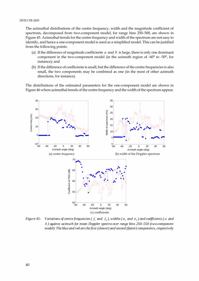
DSTO-TR-2455
40
The azimuthal distributions of the centre frequency, width and the magnitude coefficient of spectrum, decomposed from two-component model, for range bins 250–500, are shown in Figure 45. Azimuthal trends for the centre frequency and width of the spectrum are not easy to identify, and hence a one-component model is used as a simplified model. This can be justified from the following points:
(a) If the difference of magnitude coefficients a and b is large, there is only one dominant component in the two-component model (in the azimuth region of -60° to -50°, for instance); and
(b) If the difference of coefficients is small, but the difference of the centre frequencies is also small, the two components may be combined as one (in the most of other azimuth directions, for instance).
The distributions of the estimated parameters for the one-component model are shown in Figure 46 where azimuthal trends of the centre frequency and the width of the spectrum appear.
-60 -40 -20 0 20 40 60-10
0
10
20
30
40
Azimuth angle (deg)
Cen
tre fr
eq (H
z)
-60 -40 -20 0 20 40 600
5
10
15
20
25
30
35
Azimuth angle (deg)
Wid
th o
f spe
ctru
m (H
z)
(a) centre frequency (b) width of the Doppler spectrum
-60 -40 -20 0 20 40 6050
55
60
65
70
Azimuth angle (deg)
Coe
ffici
ent o
f PSD
(dB)
(c) coefficients
Figure 45: Variations of centre frequencies ( 1f and 2f ), widths ( 1σ and 2σ ) and coefficients ( a and b ) against azimuth for mean Doppler spectra over range bins 250–550 (two-component model): The blue and red are the first (slower) and second (faster) components, respectively

DSTO-TR-2455
41
-60 -40 -20 0 20 40 600
5
10
15
20
25
Azimuth angle (deg)
Cen
tre fr
eq (H
z)
-60 -40 -20 0 20 40 600
5
10
15
20
25
Azimuth angle (deg)
Wid
th o
f spe
ctru
m (H
z)
(a) Centre frequency (b) Width of the Doppler spectrum
Figure 46: Variations of centre frequency and width of the spectrum against azimuth for mean Doppler spectra over range bins 250–550 (one-component model)
The centre frequency and the width of the spectrum shown in Figure 45 and Figure 46 are for the mean spectrum over range bins 250–550. The fluctuations of the centre frequency and the width of the spectrum from range bin to range bin are shown in Figure 47. It can be seen that the centre frequency of the Doppler spectrum varies from range bin to range bin, even though the look azimuth is the same. The width of the spectrum also randomly varies, which is consistent with the random variation of correlation time shown in Figure 37 (the correlation time is inversely proportional to the width of the spectrum).
250 300 350 400 450 500 5500
5
10
15
20
25
30
35
Range bin
Cen
tre D
oppl
er fr
eq (H
z)
250 300 350 400 450 500 5505
10
15
20
25
30
35
Range bin
Wid
th o
f Spe
ctru
m (H
z)
(a) centre frequency (b) width of spectrum
Figure 47: Distribution of centre frequency and the width of the Doppler spectrum for range bins 250–550 at 0° azimuth
Based on the above observations, the following points can be drawn:
1. Both the centre frequency and the width of the Doppler spectrum vary from range bin to range bin even at the same azimuth.
2. The highest Doppler frequency does not seem to align with the upwind direction, but in some other direction. It is speculated that this might be due to the current of the ocean. If the centre frequency variation shown in Figure 46 (a) is approximated as a sinusoidal

DSTO-TR-2455
42
variation peaked at about -5°, then this direction might be the direction of the current. The associated velocity of the current is,
cc fv2
(33)
where cf is the Doppler frequency and the wavelength of radar. Given 23.0 m
and cf 18 Hz, the resultant velocity of the current is 2.1m/s. If the backscatter is modulated by a wind wave, according to the deep-water dispersion equation (Pond and Pickard, 1983), the associated wavelength c of the wave is,
22cc v
g
(34)
where g is the gravitational acceleration constant. The wavelength c varies as a
function of the Doppler frequency cf as shown in Figure 48. It can be seen that for
cf <10 Hz, the corresponding wavelengths are only in a range of centimetres to
decimetres, which relate to as ripples and capillary waves. Even when cf reaches
15–20 Hz, the corresponding wavelength is only 2–3 m, belonging to the category of short wind waves.
0 5 10 15 200
1
2
3
4
Doppler frequency (Hz)
Wav
elen
gth
(m)
Figure 48: Wavelength c varies as a function of the Doppler frequency cf
On the other hand, we may use the Pierson-Moskowitz spectrum to determine the dominant waves developed by wind in a fully developed open sea. The P-M formula is (Pierson and Moskowitz, 1964, Stewart, 2006),
4
05
2
exp)(
g
S (35)
where F 2 , F is the wave frequency in Hertz, 3101.8 , 74.0 ,
5.190 /Ug and 5.19U is the wind speed at a height of 19.5 m above the sea surface. For
most air flow over the sea the atmospheric boundary layer has nearly neutral stability,

DSTO-TR-2455
43
and 105.19 026.1 UU (Stewart, 2006), so there is not much difference between wind
speed measured at 10 m or 19.5 m above the sea surface. The P-M spectrum for a wind speed of 4.7 m/s is shown in Figure 49 where the dominant wave frequency is
33.0)2/( 5.190 UgF Hz.
0 0.2 0.4 0.6 0.80
0.002
0.004
0.006
0.008
0.01
0.012
Frequency (Hz)
Wav
e en
ergy
spe
ctra
l den
sity
(m2 /H
z)
Figure 49: Pierson-Moskowitz wave spectra for a fully developed sea at a wind speed of 4.7 m/s
The wave frequency (not to be confused with the Doppler frequency) for a wave with a wavelength c is (Pond and Pickard, 1983),
2/156.1/ cF (36) To summarise, for a fully developed sea, a wind speed of 4.7 m/s would generate in the upwind direction a dominant wave with a wave frequency of 0.33 Hz, and the wave would have a wavelength of 14.3 m. If the propagation of the wave is observed, the corresponding Doppler frequency would be 41 Hz. Therefore, the event of the scatterers modulated by dominant long wind waves was not observed. This probably explains why the highest Doppler is not in line with the upwind direction.
3. Since the correlation time is inversely proportional to the width of the spectrum, the correlation time in the upwind and crosswind directions should be longer than at other directions, which is consistent with the maps of correlation times shown in Figure 37. In fact if the Doppler spectrum (PSD) is assumed to the one-component Gaussian, then the temporal correlation is also a Gaussian (Lee, et al, 1995), as,
20 )2/exp(|)(| ttt (37)
where 10
st . Given s 6, 10, and 20 Hz, typical values of the width of Doppler
spectrum shown in Figure 46 (b), the corresponding correlation time will be 0.33, 0.2 and 0.1 s, respectively. The correlation time calculated by (37) seems to be much longer than the direct calculation in the time domain. Two factors may contribute to this discrepancy. One is an insufficient sampling time, which also causes the inaccuracy in the direct calculation as mentioned previously. The other is the assumption of the Doppler spectrum, where the true spectrum may not be a Gaussian distribution.
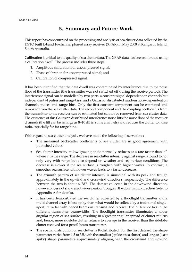
DSTO-TR-2455
44
5. Summary and Future Work
This report has concentrated on the processing and analysis of sea clutter data collected by the DSTO built L-band 16-channel phased array receiver (XPAR) in May 2008 at Kangaroo Island, South Australia. Calibration is critical to the quality of sea clutter data. The XPAR data has been calibrated using a calibration dwell. The process includes three steps:
1. Amplitude calibration for uncompressed signal;
2. Phase calibration for uncompressed signal; and
3. Calibration of compressed signal. It has been identified that the data dwell was contaminated by interference due to the noise floor of the transmitter (the transmitter was not switched off during the receive period). The interference signal can be modelled by two parts: a constant signal dependent on channels but independent of pulses and range bins, and a Gaussian distributed random noise dependent on channels, pulses and range bins. Only the first constant component can be estimated and removed from the sea clutter data. The second component and the coupling coefficients from the transmitter to the receiver can be estimated but cannot be removed from sea clutter data. The existence of this Gaussian distributed interference noise lifts the noise floor of the receiver channels (the lift can be as large as 8–10 dB in some channels) and reduces the clutter to noise ratio, especially for far range bins. With regard to sea clutter analysis, we have made the following observations:
The measured backscatter coefficients of sea clutter are in good agreement with published values.
Sea clutter intensity at low grazing angle normally reduces at a rate faster than 4r where r is the range. The decrease in sea clutter intensity against range is found to not only vary with range but also depend on weather and sea surface conditions. The decrease is slower if the sea surface is rougher, with higher waves. In contrast, a smoother sea surface with lower waves leads to a faster decrease.
The azimuth pattern of sea clutter intensity is sinusoidal with its peak and trough approximately in the upwind and crosswind directions, respectively. The difference between the two is about 6–7dB. The dataset collected in the downwind direction, however, does not show an obvious peak or trough in the downwind direction (refer to Appendix A for details).
It has been demonstrated the sea clutter collected by a floodlight transmitter and a multi-channel array is less spiky than what would be colleted by a traditional single-aperture radar with pencil beams in transmit and receive. The difference lies in the different transmitter beamwidths. The floodlight transmitter illuminates a wider angular region of sea surface, resulting in a greater angular spread of clutter returns and, hence, more sidelobe clutter returns to average in the receiver than the sidelobe clutter received for a pencil-beam transmitter.
The spatial distribution of sea clutter is K-distributed. For the first dataset, the shape parameter varies from 1.5 to 7.5, with the smallest (spikiest sea clutter) and largest (least spiky) shape parameters approximately aligning with the crosswind and upwind

DSTO-TR-2455
45
directions, respectively. The analysis of the second dataset shows the shape parameter varies from 8.5 aligning with the downwind direction to either smaller or larger in other directions.
Sea clutter in range whose range separation is greater than the radar’s range resolution is generally spatially uncorrelated. Similarly, sea clutter in azimuth is also spatially uncorrelated if the azimuth separation is greater than the radar’s azimuth resolution. Long-term spatial correlation reveals sea wave structures in range. A detailed study will be difficult, as the correlation is dependent on the number of samples used in the averaging processing. The oscillation of correlation coefficients gradually fades with an increase in the number of samples used in the averaging processing (This might suggest that the lengths of periodic waves/swells are limited, i.e., a certain periodic wave only exists in a certain range and disappears in other ranges).
The temporal correlation time of sea clutter is dependent on the environmental parameters. The mean correlation time is about 20 ms and longer than 100ms for first and second datasets, respectively. Sea clutter in the upwind direction and crosswind directions tends to have a longer correlation time.
The temporal distribution of sea clutter is Rayleigh (for amplitude distribution) or exponential (for intensity distribution). If the observation time is short and only in the order of or a few multiples of correlation time, the mean may not be estimated accurately, and the resultant distribution appears to be narrower than the Rayleigh distribution. It is anticipated that if the observation time is of the order of seconds, the distribution would be Rayleigh. If the observation time is very long and on the order of tens of seconds or longer, the distribution will become the K-distribution, as the underlying mean of sea clutter has varied due to the propagation of sea waves.
The Doppler spectrum of sea clutter is a function of both radar and environmental parameters. The Doppler spectrum of vertically polarised sea clutter has often been modelled by two Gaussian distributed components, one for the Bragg scattering and the other for the whitecap scattering. Due to limited frequency resolution (about 10 Hz) of the dataset, only a single dominant component was observed and hence the spectrum can be represented by a single Gaussian component representing the aggregate Doppler of backscatter. Statistically the centre frequency varies in a range of 0 to 20 Hz for the first dataset when the angle between the boresight of XPAR and the upwind direction is an acute angle, and has an approximately sinusoidal pattern in the azimuth with its peak in some other direction, possibly the current direction, rather than the upwind direction. For the second dataset the angle between the boresight of XPAR and the downwind direction is an acute angle, and the centre frequency varies from 0 to -6 Hz. Again the maximum Doppler (negative value) does not align with the downwind direction. The measured Doppler frequencies are low, suggesting that the scatterers move slower than the propagation of dominant wind waves. In addition the maximum Doppler does not happen in the upwind / downwind directions. The width of spectrum varies, typically from 6 to 22 Hz for the two datasets studied. It has narrower widths in the upwind and crosswind wind directions, indicating that the sea clutter has a longer correlation time in these two directions than others, consistent with the correlation study in the time domain.

DSTO-TR-2455
46
Future work:
In future trials, the transmitter should be switched off between pulses, to eliminate interference due to the transmitter’s noise floor in the receiving channel—this exists in the all current datasets.
The faulty component which caused the abnormal performance of channel 7 needs to be identified and replaced.
It has been seen in some datasets (not shown in this report) that amplitudes of the received pulses (uncompressed) oscillate. The problem needs to be further investigated.
Data with longer observing durations will be collected/processed in the future to improve the correlation and Doppler spectrum analysis and further lead to the time-frequency analysis.
6. Acknowledgment
The authors thank all members of the trial team. It was impossible to collect the trial data without their support. Drs Luke Rosenburg and Mark Preiss of Intelligence, Surveillance and Reconnaissance Division (ISRD) made detailed comments, various suggestions and many grammar corrections during the review processing. Dr Leigh Powis also made helpful comments for the first draft. Their valuable work is particularly acknowledged.
7. References
Anderson, S J, and Morris, J T, “Aspect dependence of the polarimetric characteristics of sea clutter: II. Variation with azimuth angle”, Proceeding of 2008 International Conference on Radar, pp. 608–612. Antipov, I. (1998), "Simulation of sea clutter returns", Technical Report, DSTO-TR-0679, Defence Science and technology Organisation, Australia. Billingsley, J B, Low-Angle Radar Land cluter: Measurements and Empirical Models, New York, William Andrew Publishing, 2002. Blacknell, D, “Comparison of parameter estimators for K-distribution”, IEE Proc. Radar, Sonar and Navig., 141 (1), pp. 45–52, 1994. Chan, H C, “Radar sea clutter at low grazing angles”, IEE Proceedings, Pt F, 137 (2), pp. 102–112, 1990. Conte, E, De Maio, A, and Galdi, C, “Statistical analysis of real clutter at different range resolutions”, IEEE Trans on AES, 40, (3), pp. 903–918, 2004.
DSTO-TR-2455
47
Crisp, D J, Stacy, N J S, and Goh, A S, “Ingara medium-high incidence angle polarimetric sea clutter measurements and analysis”, Technical Report, DSTO-TR0-1818, 2006. Crisp, D J, Rosenberg, L, Stacy, N J, and Dong, Y, “Modelling moderate grazing angle X-band ocean backscatter with the K-distribution”, Submitted to International Radar Conference 2009. Dong, Y, “High grazing angle and high resolution sea clutter: correlation and polarisation analyses”, Technical Report, DSTO-TR-1972, 2007. Dong, Y, and Crisp, D, “Comparison of estimation schemes for the K-distribution shape parameter”, to appear in Proceedings of 2009 International Radar Conference. Dong, Y, and Merrett, D, “Statistical measures of S-band sea clutter and targets”, technical report, DSTO-TR-2221, 2009. Farina, A, Gini, F., Greco, M V, and Verrazzani, L, “High resolution sea clutter data: statistical analysis of recorded live data”, IEE Proc. Radar, Sonar and Navig., 144, (3), pp. 121–130, 1997. Greco, M, and Gini, F, “Sea-clutter at high range resolutions and very low grazing angles”, IEEE Trans on AES, 38 (1), pp. 58–73, 2002. Greco, M, and Gini, F, “Sea-clutter nonlinearity: The influence of long waves” in Haykin, S (editor) Adaptive Radar Signal Processing, pp. 159–191, New York John Wiley and Sons, 2007. Haykin, S, Adaptive Filter Theory, 4th edition, New Jersey, Prentice Hall, 2002. Haykin, S, Bakker, R, and Currie, B W, “Uncovering nonlinear dynamics – the case study of sea clutter”, IEEE Proceedings, 90 (5), pp 860-881, 2002. Helmken, H F, “Low-grazing-angle radar backscatter from the ocean surface”, IEE Proceedings, Pt. F, 137 (2), pp. 113–117, 1990. Lee, P H Y, Barter, J D, Beach, K L, Hindman, C L, Lake, B M, Rungaldier, H, Shelton, J C, Williams, A B, Yee, R, and Yuen, H C, “X band microwave backscattering from ocean waves”, Journal of Geophysical Research (Ocean), 100 (C2), pp. 2591-2611, 1995. Lee, P H Y, Barter, J D, Caponi, E, Caponi, M, Hindman, C L, Lake, B M and Rungaldier, H, “Wind-speed dependence of small-grazing-angle microwave backscatter from sea surfaces”, IEEE Trans on Antenna and Propagation, 44 (3), pp. 333–340, 1996. Lee, P H Y, Barker, J D, Beach, K L, Lake, B M, Rungaldier, H, Thompson, Jr., H R, and Yee, R, “Scattering from breaking gravity waves without wind”, IEEE Trans on Antenna and Propagation, 46 (1), pp. 14–26, 1998. Lewis, B L, Kretschmer, Jr., F F, and Shelton, W W, Aspects of Radar Signal Processing, Dedham, Massachusetts, Artech House, 1982. Long, M W, Radar Reflectivity of Land and Sea, 3rd edition, New York, Artech House, 2001.
DSTO-TR-2455
48
Nathanson, F E, Reilly, J P, and Cohen, M N, Radar Design Principles Signal Processing and the Environment, SciTech Publishing Inc., 1999. Pierson W J, and Moskowitz, L, “A proposed spectral form for fully developed wind seas based on the similarity theory of S. A. Kitaigorodskii”, J Geophys. Res., 69 (24), pp. 5181–5190, 1964. Plant, W J, and Keller, W C, “Evidence of Bragg scattering in microwave Doppler spectra”, Journal of Geophysical Research, 95 (c5), pp. 16299–16310, 1990. Pond, S, and Pickard, G L, Introductory Dynamical Oceanography, 2nd edition, Amsterdam, Elsevier Butterworth-Heinemann, 1983. Posner, F L, “Spiky sea clutter at high range resolutions and very low grazing angles”, IEEE Trans on AES, 38, (1), pp. 58–73, 2002. Rangaswamy, M, Weiner, D, and Ozturk, A, “Non-Gaussian random vector identification using spherically invariant random processes”, IEEE Trans on AES, 29 (1), pp. 111–124, 1993. Skolnik, M I (editor in chief), Radar handbook, 2nd edition, New York, McGraw-Hill, 1990. Stewart, R H, http://oceanworld.tamu.edu/resources/ocng_textbook/chapter16/ chapter16_04.htm, 2006. Walker, D, “Experimentally motivated model for low grazing angle radar Doppler spectra of the sea surface”, IEE Proc. Radar, Sonar and Navig, 147 (3), pp. 114–120, 2000. Walker, D, “Doppler modelling of radar sea clutter”, IEE Proc. Radar, Sonar and Navig, 148 (2), pp. 73-80, 2001. Ward, K D, Tough, R J A, and Watts, S, Sea Clutter: Scattering the K Distribution and Radar Performance, Institute of Engineering Technology, 2006. Watts, S, “Radar detection statistics in spatially correlated sea clutter”, Statistical Signal Processing, IEE Colloquium on 6 Jan 1999. Wetzel, L B, “Sea clutter” in Skolnik (chief editor) Radar Handbook (3rd edition), Chapter 15, New York, McGraw-Hill, 2008. Wirth, W-D, Radar Techniques Using Array Antennas, London, IEE, 2001.

DSTO-TR-2455
49
Appendix A: Another Dataset Studied
This Appendix briefly summarises the results of another dataset, kix022. The dataset kix022 was collected on May 14 2008 at 10:06AM local time. Parameters of weather and waves recorded for kix022 are given in Table A1. Compared to the parameters of kix040 collected three days later, the differences in average wave direction and average wind speed for the two datasets were small. The differences in wind direction, the gust speed and the maximum wave height were significant. The angle between the boresight direction of XPAR and the downwind direction is shown in Figure A-I (note that the wind direction is defined ‘originated from’). XPAR therefore generally looked in downwind direction. Table A1: Parameters of weather and ocean wave for dataset kix022
Dataset Average wind
direction wrt
North (°)
Relative to
boresight of array
(°)
Average wave
direction wrt to
North (°)
Average wind speed (m/s)
Gust speed (m/s)
Tempe-rature (°C)
Significant wave height
moH (m)
Max wave height
maxH (m)
kix022 340 162 231 4.5 7.2 15.0 2.4 3.4
Ch 1 Ch 16
Boresightdirection
o178
Winddirection
o340
N
N
162o
Figure A1: Angle between the upwind and boresight directions
The noise floor of the calibration dwell, i.e., without the interference of the transmitter’s noise floor is plotted in Figure A2. Compared with Figure 10, it can be seen that both datasets have a similar noise floor distribution, the difference between the corresponding channels is less than 0.5 dB.

DSTO-TR-2455
50
2 4 6 8 10 12 14 16-22
-20
-18
-16
-14
-12
-10
Channel
Rel
ativ
e no
ise
leve
l (dB
)
Figure A2: Relative noise floor levels without the transmitter interference
Profiles of the constant interference component from the transmitter for range bins 1500, 1600, 1700, 1800 and 1900, respectively, are shown in Figure A3. A profile of the mean constant interference component averaged over range bins 1500 to 2000 is also shown in the figure. Again it can be seen that the constant interference signal is independent of range bins. The pattern and the level of the noise are however different from what is shown in Figure 16, which is understandable, as the relative positions between the transmitter and XPAR were different due to different stopping positions of the van (the transmitter was on the top of the van) on different days.
2 4 6 8 10 12 14 16-40
-30
-20
-10
0
Channel
Rel
ativ
e si
gnal
leve
l (dB
)
Bin 1500Bin 1600Bin 1700Bin 1800
Bin 1900Av e ofBins 1500-2000
Figure A3: Constant interference signal dependent on channels but independent of range bins
The profile of the relative noise floor of the data dwell after the removal of the constant interference signal is shown in Figure A4. Compared to Figure A3, it is seen that they both have a similar pattern, especially for channels that have higher noise levels dominated by the interference, as both the constant and random interference signals were coupled from the transmitter to XPAR via the same medium. The increase of the noise level for each channel due to the interference from the transmitter can be estimated by comparing Figures A4 and A2. For instance, the relative noise levels with and without the interference for channel 8 are

DSTO-TR-2455
51
approximately -18 dB and -18.5 dB, respectively, indicating a 0.5 dB increase in the noise level. Similarly one can find that the increase for channel 9 is about 8.5 dB.
2 4 6 8 10 12 14 16-20
-18
-16
-14
-12
-10
-8
Channel
Rel
ativ
e no
ise
leve
l (dB
)
Figure A4: Relative noise levels of XPAR after the removal of the constant interference signal. The
profile is averaged over range bins from 1500 to 2000 and 512 pulses.
Single channel clutter range profiles are shown in Figure A5. Compared to Figure 21, one sees that apart from different noise floor levels for different channels, the sea clutter profiles of kix022 drop much faster than that of kix040. A comparison of mean clutter range profiles for kix022 and kix040 is shown in Figure A6, from which it can be seen that the sea clutter approximately approaches the noise floor at range bin 650 for kix022 whereas it does not drops to the noise floor till range bin 850 for kix040. Since the radar parameters are the same, the differences must be attributed to changes in weather and ocean waves. The main differences included the wind direction and the gust speed. For kix040 the angle between the boresight of XPAR and the upwind direction was an acute angle of 52°, so the radar viewed the sea surface in the upwind direction. On the other hand, the angle was 162° for kix022, so the radar viewed the sea surface in the downwind direction. The gust wind was also significantly stronger for kix040 (25 m/s against 7.2 m/s). Also the difference was the maximum wave heights (6.6 m for kix040 against 3.4 m for ki022). It is thus anticipated that the sea surface was rougher for kix040 resulting in higher sea clutter, and a slower decrease against range.

DSTO-TR-2455
52
0 500 1000 1500 2000-30
-20
-10
0
10
20
30
40
50
Range bin
Rel
ativ
e si
gnal
leve
l (dB
)
Sea clutter
Noise f loors
Unknow n target
Transmitter pulse
Figure A5: Clutter range profiles of individual channels after the removal of the constant interference
signal. The profiles are averaged by 512 pulses.
0 200 400 600 800 1000-20
-10
0
10
20
30
40
Range bin
Rel
ativ
e se
a cl
utte
r int
ensi
ty (d
B)
Unknow ntargets
Delayedtransponder
Transmitter pulse
Kix022
Kix040
Figure A6: Comparison of sea clutter range profiles of kix040 and kix022
The azimuth-range clutter maps before the removal of the range dependent intensity and the compensation of beam azimuthal patterns of transmitter and receiver are shown in Figure A7. Two unknown targets located at range bin 579 with an azimuth angle -39° (it was seen in the kix040) and range bin 257 with azimuth angle -52° are also seen in the range profile in Figure A6. The delayed transponder was not used in this dataset.

DSTO-TR-2455
53
(a) Uniform window (b) 35dB Chebyshev window
Figure A7: Azimuth-range clutter maps resulted from (a) a uniform window and (b) a 35 dB Chebyshev window
The curve of intensity dropping against range found for sea clutter dominant range bins 250 to 450 is shown in Figure A8. Equation (18) was used to approximate the curve with the following parameters: 5.40 , 3 , 2501 r and 4502 r . The corresponding grazing angles and the
associated range factor are given in Table A2. Comparing Table A2 and Table 3, it becomes obvious that the dropping pattern is dependent on the weather and sea surface conditions even though the observation geometry and radar parameters remain unchanged.
0 100 200 300 400 500 600 700 800 900-20
-10
0
10
20
30
40
Range bin
Rel
ativ
e si
gnal
leve
l (dB
)
Figure A8: Sea clutter range profile averaged over 512 pulses and 16 channels in blue. The green curve
is the approximated intensity dropping curve.
Table A2: Range, grazing angle and Range factor
Range bin Range (m) Grazing angle (°) Range factor 250 2100 1.66 5.4r 450 4500 0.78 8.4r
The multi-channel sea clutter range profiles after the removal of the range effect for range bins 270–450 is shown in Figure A8. The choice of the region is to exclude the unknown target in range bin 257 and its neighbouring bins in the near range. The far range bin of the region is limited by the available bins containing dominant sea clutter.

DSTO-TR-2455
54
300 350 400 450-30
-20
-10
0
10
Range bin
Rel
ativ
e si
gnal
leve
l (dB
)
Figure A9: Sea clutter range profiles of 16 channels after removal of range effect
Figures A10 (a) and (b) show the sea clutter azimuthal distributions for range bins 270–450 before and after the compensation of the beam patterns. Their mean curves are also shown in the figure. The azimuth-range map of sea clutter is shown in Figure A11.
-90 -60 -30 0 30 60 90-30
-20
-10
0
10
20
30
Azimuth angle (deg)
Rel
ativ
e si
gnal
leve
l (dB
)
-60 -40 -20 0 20 40 60
-20
-10
0
10
20
30
Azimuth angle (deg)
Rel
ativ
e si
gnal
leve
l (dB
)
(a) before beam pattern is removed (b) after beam pattern is removed
Figure A10: Sea clutter azimuthal distributions for range bins 270 to 450. The thick blue curves are the corresponding mean clutter.
Azimuth angle (deg)
Ran
ge b
in
-60 -40 -20 0 20 40 60
280
300
320
340
360
380
400
420
440
-40
-30
-20
-10
0
10
20
Figure A11: Azimuth-range map of sea clutter after removal of the range effect and azimuth beam
pattern

DSTO-TR-2455
55
The mean curve shown in Figure A10 (b) is replotted in Figure A12 and the downwind direction relative to the boresight of the XPAR is indicated. According to a previous study (Crisp, at al, 2006), the sea clutter azimuth distribution often shows a second peak aligning with the downwind direction. The peak is lower than the first peak aligning with the upwind direction, but higher than the troughs aligning with the crosswind directions. Such a pattern is not observed in this dataset.
-60 -40 -20 0 20 40 6010
11
12
13
14
15
16
Azimuth angle (deg)
Rel
ativ
e m
ean
clut
ter (
dB)
Dow nw inddirection
Figure A12: Azimuth distribution of relative mean clutter
The spatial distribution of sea clutter in range bins 270 to 450 at azimuth -60° to 60°, after the removal of the range effect and the compensation of the beam patterns, is again assumed to be K-distributed. The variation of the estimated shape parameter with the azimuth angle is given in Table A3. It can be seen that the estimated shape parameter varies significantly. The symmetrical directions with respect to the downwind direction do not have the similar shape parameters. Instead, the shape parameter varies from being small at -50° to large at 50°. Table A3: Shape parameter against azimuth direction (the downwind direction is = 18°)
Azimuth -50°≤≤-30° -30°≤≤-10° -10°≤≤10° 10°≤≤30° 30°≤≤50° -60°≤≤60° Shape
parameter 2.85 8.54 7.78 50 43.7 5.1
The azimuth-range maps of correlation time are shown in Figure A13 (a) and (b) calculated by the use of || and )( , respectively. Given a total 512 pulses (about 100 ms), most pixels in figure A13 (a) has a correlation time of 100ms which means that the correlation coefficient never drops to 1/e for the length of sampling time considered. Therefore more pulse samples are needed in order to increase the calculation accuracy. The differences between the two maps are obvious, and reasons have been given previously. Compared to the correlation time of kix040, statistically kix022 has a much longer correlation time. The corresponding histograms of the calculated correlation time are shown in Figure A14. As shown when the correlation time is based on || , it has a dominant component of 100 ms, whereas when it is based on )( , it has a cluster in 30 ms but also has a significant component of 100 ms. According to the environmental parameters, the sea surface of ki022 should be much smoother than that of ki040, resulting in a longer correlation time. Again the last significant bar of 100 ms should be understood as the sum of the histograms equal to and greater than 100 ms.
Downwind direction

DSTO-TR-2455
56
Azimuth angle (deg)
Ran
ge b
in
-60 -40 -20 0 20 40 60
280
300
320
340
360
380
400
420
440
0
20
40
60
80
100
Azimuth angle (deg)
Ran
ge b
in
-60 -30 0 30 60
280
300
320
340
360
380
400
420
440
0
20
40
60
80
100
(a) calculated by use of || (b) calculated by use of )(
Figure A13: Range-azimuth maps of temporal correlation time in milliseconds calculated by use of (a) || and (b) )( .
0 50 1000
0.05
0.1
0.15
0.2
0.25
0.3
Azimuth angle (deg)
0 20 40 60 80 1000
0.02
0.04
0.06
0.08
0.1
Correlation time (ms)
(a) calculated by use of || (b) calculated by use of )(
Figure A14: Distribution of the correlation time for sea clutter in range bins 270–450 at azimuth of -60° to +60°. The distribution in (a) has a dominant component at 100 ms, whereas in (b) it has a cluster centred at 30 ms plus a large component at 100 ms.
The temporal distribution for the normalised sea clutter intensity (with respect to pulses) is shown in Figure A15. Again the distribution is narrower than the exponential distribution due to the inaccurate estimation of the mean. Since the correlation time is longer, the number of equivalent iid looks in 512 pulse samples is even smaller for ki022 which explains why the shape of the pdf of ki022 is even narrower than that of ki040. It is anticipated that the distribution would be exponential if the sampling time is longer to allow the mean to be estimated more accurately.

DSTO-TR-2455
57
-30 -20 -10 0 100
0.05
0.1
0.15
0.2
Normalised clutter intensity (dB)
-60 -40 -20 010
-6
10-4
10-2
100
Clutter intensity (dB)
(a) (b)
Figure A15: Temporal distribution of sea clutter in range-azimuth bins, the data’s pdf in blue line-circle compared with the exponential distribution in green line. The pdfs are plotted on (a) linear scale to view the global distribution and (b) log scale to view the tails’ distribution.
The Doppler-range map of sea clutter in range bins 270–450 at 0° azimuth is shown in Figure A16. It is seen that in general only one Doppler component dominates for each range bin. Figure A17 plots the Doppler spectra of sea clutter for range bins 270–450 at 0° azimuth. In fact both figures A16 and A17 show the same information, but in the latter range bins become indiscriminative.
Doppler freq (Hz)
Ran
ge b
in
-100 -50 0 50 100
300
350
400
450
-20
0
20
40
60
Figure A16: Doppler-range map of sea clutter for range bins 270–450 at 0° azimuth
-500 -250 0 250 500-20
0
20
40
60
80
Doppler freq (Hz)
Rel
ativ
e PS
D (d
B)
Figure A17: Doppler spectra of sea clutter for range bins 270–450 at 0° azimuth

DSTO-TR-2455
58
The mean Doppler spectrum of sea clutter over range bins 270–450 at 0° azimuth is shown in Figure A18, together with the fits of both the two-component and one-component models, respectively. The figure is plotted on the linear and log scales in the first and second rows, respectively, for each model. The associated estimated model parameters are given in Table A4. It can be seen that although the fit of the one-component model is not as good as the two-component model, the result is acceptable. The one-component model considers the aggregate Doppler of sea clutter. Compared to Figure 44 for kix040, the width of the Doppler spectrum of kix022 shown in Figure A18 is narrower. In the time domain, the correlation time for kix022 is longer. Physically the sea surface of the kix022 was smoother and the sea waves were lower.
-100 -50 0 50 1000
1
2
3
4x 10
6
Doppler frequency (Hz)
Rel
ativ
e PS
D o
n lin
ear s
cale
-100 -50 0 50 1000
1
2
3
4x 10
6
Doppler frequency (Hz)
Rel
ativ
e PS
D o
n lin
ear s
cale
-500 -250 0 250 50020
30
40
50
60
70
Doppler frequency (Hz)
Rel
ativ
e PS
D o
n lo
g sc
ale
-500 -250 0 250 50020
30
40
50
60
70
Doppler frequency (Hz)
Rel
ativ
e PS
D o
n lo
g sc
ale
(a) Two-component model (b) One-component model
Figure A18: The goodness-of-fit of (a) two-component model and (b) one-component model to the mean Doppler spectrum of sea clutter in range bins270–450 at 0° azimuth. The blue dotted curve is the measurement and the green curve is the model fit.
Table A4: Estimated parameters for the mean Doppler spectrum of sea clutter in range bins 270–450 at
0° azimuth
Parameter a (dB) 1f (Hz) 1s (Hz) b (dB) 2f (Hz) 2s (Hz) 2n (dB)* Two-component model 65.0 -9.39 6.26 63.9 0.38 6.00 27.5 One-component model 65.4 -5.51 10.30 - - - 27.5
* a , b and 2n are relative values.
Variations of the Doppler centre frequency and the width of spectrum against azimuth for the mean Doppler spectra of sea clutter in range bins 270–450 are shown in Figure A19. The centre of the trough of centre frequency shown in Figure A19 does not coincident with the downwind direction. There might be two possibilities. One is the downwind direction measured at the island not necessarily consistent with the actual downwind direction on the sea surface where

DSTO-TR-2455
59
the sea clutter was collected. The other is that there existed a current whose direction was different from the upwind direction. Nevertheless, the centre frequency of the Doppler in the downwind direction is about -5 Hz which then tends to 0 Hz in the cross-wind directions. Again these centre frequencies of Doppler cannot be directly linked the propagation velocities of the dominant sea waves. The Doppler frequencies of dominant sea waves, if observed, would be much faster, so the so-called fast event was not observed. The figure also shows that when the centre frequency approaches to zero hertz, the associated width of spectrum also becomes smaller (the similar situation was also observed for ki040). This implies that for these directions, the correlation time of sea clutter is longer. Since the correlation time is inversely proportional to the width of the spectrum (see (37)), if the width of spectrum is reduced to a half, the corresponding correlation time would be doubled.
-60 -40 -20 0 20 40 60-8
-6
-4
-2
0
2
Azimuth angle (deg)
Cen
tre fr
eq (H
z)
Dow nw inddirecion
-60 -40 -20 0 20 40 600
2
4
6
8
10
12
Azimuth angle
Wid
th o
f spe
ctru
m (H
z)
(a) Centre frequency (b) Width of the Doppler spectrum
Figure A19: Variations of centre frequency and width of spectrum against azimuth for mean Doppler spectra of range bins 270–450 (one-component model)

DSTO-TR-2455
60

DSTO-TR-2455
61
Appendix B: Genetic Algorithm and Particle Swarm
B.1. Genetic Algorithm
A genetic algorithm (GA) offers an alternative to solve optimisation problems (often with multiple variables and complicated functions). It is an optimisation algorithm inspired by the well-known biological processes of genetics and evolution (Haupt and Werner, 2007). Genetics is the study of the inheritance, evolution and variation of biological traits. Genetics and evolution result in a population that is adapted to succeed in its environment. In another words, the population is optimised for its environment. Numerical optimisation of GA is analogous to genetics in that they both seek to find better results within constraints on the variables. In general, a GA involves following steps:
1. Generate a random population consisting of a group of chromosomes. Each chromosome is composed of genes or variables;
2. Evaluate the fitness of each population member;
3. Invoke natural selection;
4. Select members for mating;
5. Generate offsprings from the parenting generation;
6. Mutate selected members;
7. Evaluate the fitness of the new generation of the population;
8. Terminate run or go to step 2. B.2. Particle Swarm
Particle swarm (PS) is an algorithm for finding optimal solutions through the interaction of individuals in a swarm of particles (Kennedy and Eberhart, 2001, Clerc and Kennedy, 2002). The algorithm, which is based on the analogy of social interactions, searches a space by adjusting the trajectories of the individual vectors, called particles, toward the optimal region. Individual particles are drawn stochastically toward the positions of their own previous best performance and the previous best performance of their neighbours. PS is similar to GA in that both are initialised with a population of random solutions. The former is unlike the latter in that each potential solution is also assigned a random velocity toward a possible better solution and travels through the problem space. The PS algorithm may be expressed as (Eberhart and Shi, 2000),
1()1()1()1()1()( 21 kxkpdckxkpdckvkv igiiii Ni ,,1 (B1)
)()1()( kvkxkx iii Ni ,,1 (B2)
Where ix and iv , are respectively the position vector and velocity vector for the ith particle; N
is the size of population; ,1,0k , is the number of iteration; ip is the previous best position
vector for the ith particle, and gp is the previous best position vector for the whole population;
1d and 2d are random numbers ranging from zero to one; and 729.0 and 4945.1c are

DSTO-TR-2455
62
two constriction factors used in the iteration. These two factors are said to provide best performance for the PS algorithm (Eberhart and Shi, 2000). In addition, a limiting maxv to the
velocity and a limiting maxx to the position are also used to contain all particles within the valid
space. It has been found that in general PS outperforms GA in terms of the converging speed, possibly due to the fact that the moving trajectories of particles are partially controlled and tend towards potentially better solutions. Some researchers found that the use of a hybrid algorithm of PS and GA could accelerate the convergence for array beamforming designs (Yeo and Lu, 2005). It should be pointed out that due to the nature of both the GA and PS algorithms, reinitialising the random number generator and running the algorithms again might produce different results. Changing the parameters, such as the population size, mutation rate, constriction factors will also affect the converging speed. The nature of random variables in GA and PS and the nature of nonlinear and complexity of the goal function sometimes make the final results unpredictable. They usually generate good results, but not necessarily the globally optimal results when optimising a complicated function containing multiple local optimal positions in the variable space. Often a careful selection of initial starting points helps. Since the globally optimal point is unknown, often the algorithms are run repeatedly with different initial points and the best of them (if converging to different points) is assumed to be the best or optimal. B.3. Application of PS to Array Beamforming
We have tested both the PS and GA algorithms for array beamforming and found that PS outperformed GA. In this section we show some results of array beamforming obtained by the PS algorithm.
1 1 2 2
d=
Figure B1: A 6-element array with two independent adjustable phasers
First consider a simple example. A 6-element half-wavelength spacing linear array, as shown in Figure B1, has two independent adjustable phasers, 1 and 2 . The goal is to minimise the sum of sidelobes at three azimuth directions, sin( 30 ) , sin(20.5 ) and sin(58.2 ) . According to the basics of array antennas, the optimisation problem is written as,
2
0
5
0,
,min
21 m kkmk zw
(B-3)

DSTO-TR-2455
63
where
TjjjjT eeeeww 2112 1150 w and
mkj
km ez sin, , 5,,0k , 2,1,0m , o300 , o5.201 and o2.582
This is a two-dimensional non-linear optimisation problem. One may perform a two-dimensional search over the entire plane of 2,0 21 to allocate the globally optimal point. If the search step is 1000/2 , the goal function (B3) needs to be evaluated 106 times to find the globally optimal point of (B1). Obviously with an increase in the number of variable dimensions and the complexity of goal function, such a direct search (also called an exhaustive search) might become unfeasible. The contour of the goal function of (B3) on the variable plane is shown in Figure B2. It can be seen the goal function contains a few locally optimal points. Shown in Figure B2 (a) is a run of PS with 30 initial particles (green stars), of which the best performance is the red star on the edge of the lower left corner of the plane. A search starts from this initial condition according to the algorithms defined in (B1) and (B2) seeking better solutions than the initial best solution. The search leads to the second position on the edge of the top left corner of the plane as shown in Figure B2 (b). Repeating the search results in the converging route toward to the globally optimal point. From this illustration, it can be seen that the first two red stars in Figure B2 (b) are actually in two locally optimal regions. The PS algorithm seems to have a capability to ‘jump out’ from local optimal regions and continue to travel to the globally optimal regions and converge. It is also possible that the particles are trapped in the local optimal regions and are unable to travel to the globally optimal region. An example of this is shown in Figure B3 where the best particles were trapped in a locally optimal region and were unable to ‘jump out’. Repeat runs with different random initial conditions often able to find the optimal resolution and exclude locally optimal points. The array factor with 021 and the optimised array factor according to (B3) are shown in Figure B4.
(a) (b)
Figure B2: Contour of the goal function on the variable plane and (a) initial 30 random positions in green stars of which the best is the red star, and (b) converging route toward the globally optimal position

DSTO-TR-2455
64
Figure B3: During the iteration best particles are trapped in a locally optimal region (red stars in the
top left corner of the plane) and fail to find the globally optimal position.
-1 -0.5 0 0.5 10
1
2
3
4
5
6
Normalised azimuth
Arra
y fa
ctor
Figure B4: Array factor with 021 in blue and the array factor in green which has the minimum sum of sidelobes at the three specified azimuth directions (indicated by the three red lines).
We further demonstrate the application of PS in beamforming designs by showing a few further examples below. The beam pattern of a 32 half-wavelength spacing linear array with 35 dB Chebyshev weights is shown in Figure B5. The objective is to find a set of weights so that the sidelobe level at specified regions is a further 10 dB down, while maintaining the mainlobe width with as little change as possible. The template of the mainlobe width and the sidelobe levels to achieve is shown in red broken lines in the figure. We let the goal (cost) function be, i
mainlobeiii
Tfsidelobes
iii
iii
TfTfL
)()()()()()(
(B4)
where
1
010 )exp(log20)(N
kiki kjwf is the beam pattern value in dB and )( iT is the
template value in dB as shown in figure at azimuth direction i ( 11 i ) and kw ,
1,,0 Nk , are the optimal weights to be found in the complex domain. Equation (B4)

DSTO-TR-2455
65
shows the total loss L containing two parts. The first part counts the loss only if the sidelobe is above the template, while the second part always counts the difference. The goal is to minimise the total loss L by choosing the 32 weights in the complex domain. The optimised beam pattern through PS is also shown in Figure B5. It can be seen that the required sidelobe levels are achieved with a little broadening of the mainlobe compared to that of the 35 dB Chebyshev weights.
-1 -0.8 -0.6 -0.4 -0.2 0 0.2 0.4 0.6 0.8 1-50
-45
-40
-35
-30
-25
-20
-15
-10
-5
0
Normalised azimuth
Beam
pat
tern
(dB)
Figure B5: Original beam pattern of 32 elements with 35 dB Chebyshev weights in light blue, the goal pattern to achieve in red and the pattern in dark blue is the realisation after the PS search of weights
The next example to be shown is array failure correction using the PS algorithm. Assume element 5 of a 32 half-wavelength spacing linear array is in failure. The goal is to find a proper set of weights so that the sidelobe level is maintained approximately at -35 dB with as little increase in the broadness of the mainlobe as possible. Using the same cost function of (B4), the optimised beam pattern is found and shown in red in Figure B6, together with the original beam pattern without element failure in blue and the beam pattern with element failure in green for comparison. It can be seen that the sidelobe of the array with the element failure has been corrected and suppressed to the required level. The associated cost is a slight broadness of the mainlobe. It has been found that channel 7 of the 16-channel XPAR array did not work properly during the sea clutter collection, and therefore it is worth to investigate the array’s performance without channel 7. Since the failure element is close to the centre of a small array, it makes the correction limited and it is difficult to lower the sidelobe level even with sacrificing the mainlobe width. Figure B7 shows the beam pattern of a 16 half-wavelength spacing element array with 20 dB sidelobe Chebyshev weights, as well as the beam pattern with the failure of element 7 without weight correction. Two beam patterns using the corrected weights optimised by PS are shown in Figure B8. The difference between the two lies in a slight difference in the selection of cost function. For first result, the cost of all sidelobes is the same, so all sidelobes are minimised to approximately the same level. In the second the cost of the first sidelobe is less than the others. The actual weights for these two results are given in Table B1. The Chebyshev 20 dB sidelobe weights are also given in the table for comparison.

DSTO-TR-2455
66
-1 -0.8 -0.6 -0.4 -0.2 0 0.2 0.4 0.6 0.8 1-45
-40
-35
-30
-25
-20
-15
-10
-5
0
Normalised azimuth
Beam
pat
tern
(dB)
Figure B6: Original beam pattern of 32 elements with 35 dB Chebyshev weights in blue, the beam pattern with element 5 failure in green and the beam pattern correction with element 5 failure in red after the PS search of weights.
-1 -0.8 -0.6 -0.4 -0.2 0 0.2 0.4 0.6 0.8 1-25
-20
-15
-10
-5
0
Normalised azimuth
Beam
pat
tern
(dB)
Figure B7: Beam pattern of 16 elements with 20 dB Chebyshev weights in blue and the associated
pattern due to failure of element 7 in red.

DSTO-TR-2455
67
-1 -0.8 -0.6 -0.4 -0.2 0 0.2 0.4 0.6 0.8 1-25
-20
-15
-10
-5
0
Normalised azimuth
Beam
pat
tern
(dB)
-1 -0.8 -0.6 -0.4 -0.2 0 0.2 0.4 0.6 0.8 1
-25
-20
-15
-10
-5
0
Normalised azimuth
Beam
pat
tern
(dB)
(a) (b)
Figure B8: Results of beam pattern correction using the PS algorithm. The blue one is the 20 dB Chebyshev pattern and the template in red is the goal pattern to achieve. Two corrected beam patterns are shown in green. The differences between the two are (a) all sidelobes are minimised to the same level and (b) the first sidelobe is allowed higher than the others.
Table B1: Weights found by the PS algorithm for the corrected beam patterns shown in Figure B8.
Chebyshev 20 dB sidelobe weights are also given for comparison.
Weights for Figure B8 (a) Weights for Figure B8 (b) No Chebyshev weights Real part Imaginary
part Real part Imaginary
part 1 0.86683 0.38613 -0.02301 0.32357 -0.01743 2 0.50431 0.44367 -0.02258 0.42894 -0.02511 3 0.62167 0.55155 -0.02527 0.56066 -0.03760 4 0.73338 0.56532 -0.03307 0.58773 -0.03928 5 0.83273 0.76317 -0.03612 0.76784 -0.04493 6 0.91351 0.92307 -0.04544 0.87332 -0.05671 7 0.97052 0.0 0.0 0.0 0.0 8 1.00000 0.99872 -0.05055 0.98585 -0.05689 9 1.00000 0.94405 -0.04466 0.95916 -0.04400 10 0.97052 0.94204 -0.05250 0.99896 -0.04561 11 0.91351 0.75417 -0.03341 0.87057 -0.03482 12 0.83273 0.65980 -0.03320 0.80034 -0.03479 13 0.73338 0.51868 -0.02733 0.66689 -0.02583 14 0.62167 0.63700 -0.03155 0.70187 -0.03256 15 0.50431 0.46978 -0.02370 0.46708 -0.02350 16 0.86683 0.30429 -0.01848 0.25354 -0.01745

DSTO-TR-2455
68
B.4. References
Clerc, M, and Kennedy, J, “The particle swarm – explosion, stability, and convergence in a multidimensional complex space”, IEEE Trans on Evolutionary Computation, vol. 6, no. 1, pp. 58-73, 2002.
Eberhart, R C, and Shi, Y, “Comparison inertia weights and constriction factors in particle swarm optimisation”, Proceedings of the 2000 Congress on Evolutionary Computation, pp. 84-88.
Haupt, R L, and Werner, D H, Genetic Algorithms in Electromagnetics, New Jersey, John Wiley & Sons, 2007.
Kennedy, J, and Eberhart, R, Swarm Intelligence, Morgan Kaufmann Publishers, San Francisco, 2001.
Yeo, B-K, and Lu, Y, “Adaptive array digital beamforming using complex-coded particle swarm optimisation genetic algorithm”, Proceedings of 2005 Asia-Pacific Microwave Conference.

Page classification: UNCLASSIFIED
DEFENCE SCIENCE AND TECHNOLOGY ORGANISATION
DOCUMENT CONTROL DATA 1. PRIVACY MARKING/CAVEAT (OF DOCUMENT)
2. TITLE Analysis of L-band Multi-Channel Sea Clutter
3. SECURITY CLASSIFICATION (FOR UNCLASSIFIED REPORTS THAT ARE LIMITED RELEASE USE (L) NEXT TO DOCUMENT CLASSIFICATION) Document (U) Title (U) Abstract (U)
4. AUTHOR(S) Yunhan Dong and David Merrett
5. CORPORATE AUTHOR DSTO Defence Science and Technology Organisation PO Box 1500 Edinburgh South Australia 5111 Australia
6a. DSTO NUMBER DSTO-TR-2455
6b. AR NUMBER AR-014-829
6c. TYPE OF REPORT Technical Report
7. DOCUMENT DATE August 2010
8. FILE NUMBER 2009/1054263
9. TASK NUMBER DMO 07/102
10. TASK SPONSOR DGMSS
11. NO. OF PAGES 68
12. NO. OF REFERENCES 36
13. URL on the World Wide Web http://www.dsto.defence.gov.au/corporate/reports/DSTO-TR-2455.pdf
14. RELEASE AUTHORITY Chief, Electronic Warfare and Radar Division
15. SECONDARY RELEASE STATEMENT OF THIS DOCUMENT
Approved for public release OVERSEAS ENQUIRIES OUTSIDE STATED LIMITATIONS SHOULD BE REFERRED THROUGH DOCUMENT EXCHANGE, PO BOX 1500, EDINBURGH, SA 5111 16. DELIBERATE ANNOUNCEMENT No Limitations 17. CITATION IN OTHER DOCUMENTS Yes 18. DSTO RESEARCH LIBRARY THESAURUS http://web-vic.dsto.defence.gov.au/workareas/library/resources/dsto_thesaurus.shtml Sea clutter, L-band sea clutter, Phased array, Beamforming 19. ABSTRACT An L-band multi-channel sea clutter trial was conducted using a DSTO-built 16-channel receiving array (called XPAR) in May 2008 at Kangaroo Island, South Australia. This report presents a number of calibration techniques and analyses various properties of sea clutter including backscatter coefficient, spatial and temporal correlations, distributions and Doppler spectra. Observed phenomena are explained.
Page classification: UNCLASSIFIED