analysis of laminated glass arches and … · figure 2.3 deflection versus load for laminated glass...
TRANSCRIPT
ANALYSIS OF LAMINATED GLASS ARCHES AND CYLINDRICAL SHELLS
A THESIS SUBMITTED TO THE GRADUATE SCHOOL OF NATURAL AND APPLIED SCIENCES
OF MIDDLE EAST TECHNICAL UNIVERSITY
BY
EBRU DURAL
IN PARTIAL FULFILLMENT OF THE REQUIREMENTS FOR
THE DEGREE OF DOCTOR OF PHILOSOPHY IN
ENGINEERING SCIENCES
JANUARY 2011
Approval of the thesis:
ANALYSIS OF LAMINATED GLASS ARCHES AND CYLINDRICAL SHELLS
Submitted by EBRU DURAL in partial fulfillment of the requirements for the degree of doctor of philosophy in Engineering Sciences Department, Middle East Technical University by, Prof. Dr. Canan Özgen ________________ Dean, Graduate School of Natural and Applied Sciences Prof. Dr. Turgut Tokdemir ________________ Head of Department, Engineering Sciences Prof. Dr. M. Zülfü Aşık ________________ Supervisor, Engineering Sciences Dept., METU
Examining Committee Members:
Prof. Dr. Gülin Ayşe Birlik ________________ Engineering Sciences Dept., METU Prof. Dr. M. Zülfü Aşık ________________ Engineering Sciences Dept., METU Prof. Dr. Uğurhan Akyüz ________________ Civil Engineering Dept., METU Assoc. Prof. Dr. Hakan I. Tarman ________________ Engineering Sciences Dept., METU
Assist. Prof. Dr. Mehmet Yetmez ________________ Mechanical Engineering Dept., ZKU
Date: 12.01.2011
iii
PLAGIARISM
I hereby declare that all information in this document has been obtained and presented in accordance with academic rules and ethical conduct. I also declare that, as required by these rules and conduct, I have fully cited and referenced all material and results that are not original to this work. Name, Last Name : Ebru DURAL Signature :
iv
ABSTRACT
ANALYSIS OF LAMINATED GLASS ARCHES AND CYLINDRICAL SHELLS
DURAL, Ebru
Ph. D, Department of Engineering Sciences
Supervisor: Prof. Dr. M. Zülfü AŞIK
January 2011, 244 pages
In this study, a laminated glass unit which consists of two glass sheets bonded
together by PVB is analyzed as a curved beam and as a cylindrical shell. Laminated
glass curved beams and shells are used in architecture, aerospace, automobile and
aircraft industries. Curved beam and shell structures differ from straight structures
because of their initial curvature. Because of mathematical complexity most of the
studies are about linear behavior rather than nonlinear behavior of curved beam and
shell units. Therefore it is necessary to develop a mathematical model considering
large deflection theory to analyze the behavior of curved beams and shells.
Mechanical behavior of laminated glass structures are complicated because they can
easily perform large displacement since they are very thin and the materials with the
elastic modulus have order difference. To be more precise modulus of elasticity of
glass is about 7*104 times greater than the modulus of elasticity of PVB interlayer.
Because of the nonlinearity, analysis of the laminated glass has to be performed by
considering large deflection effects. The mathematical model is developed for curved
beams and shells by applying both the variational and the minimum potential energy
principles to obtain nonlinear governing differential equations. The iterative
technique is employed to obtain the deflections. Computer programs are developed
v
to analyze the behavior of cylindrical shell and curved beam. For the verification of
the results obtained from the developed model, the results from finite element models
and experiments are used. Results used for verification of the model and the
explanation of the bahavior of the laminated glass curved beams and shells are
presented in figures.
Keywords: Laminated Glass, large deflection, curved beam, shell, nonlinear
behavior.
vi
ÖZ
LAMİNA CAM EĞRİSEL KİRİŞ VE SİLİNDİRİK KABUKLARIN
ÇÖZÜMLEMESİ
DURAL, Ebru
Doktora., Mühendislik Bilimleri Bölümü
Tez yöneticisi: Prof. Dr. M. Zülfü AŞIK
Ocak 2011, 244 sayfa
Bu çalışmada PVB ile birbirine bağlanmış iki cam levhadan oluşan lamina cam
eğrisel kiriş ve silindirik kabuk yapının çözümlenmesi yapılmıştır. Lamina cam
eğrisel kiriş ve kabuklar mimari, havacılık, otomobil ve uçak endüstrisinde
kullanılırlar. Eğrisel kirişler ve kabuk yapılar eğrilikleri nedeniyle düzlemsel
yapılardan farklıdırlar. Matematiksel karmaşıklıkları nedeniyle yapılan çalışmaların
bir çoğu eğrisel kiriş ve kabuk elemanların doğrusal olmayan davranışlarından
ziyade doğrusal olan davranışları ile ilgilidir. Dolayısıyla eğrisel kiriş ve kabukların
davranışını çözümlemek için büyük yerdeğiştirmeler kuramını dikkate alan bir
matematiksel model geliştirilmesi gerekmektedir. Lamina cam yapılar ince olmaları
nedeniyle kolayca büyük yerdeğiştirmeler gösterdiklerinden ve malzemelerin
elastisite modülleri arasındaki büyük farktan dolayı mekanik davranışları
karmaşıktır. Daha açıklayıcı şekilde ifade edilirse camın elastisite modülü PVB
aratabakanın elastisite modülünden yaklaşık 7*104 kez daha büyüktür. Doğrusal
olamayan davranışları nedeniyle lamina camların gerçekçi çözümlemesi büyük
yerdeğiştirmelerin etkisi gözönüne alınarak yapılması gerektiğinden eğrisel kiriş ve
vii
kabukların doğrusal olmayan hakim denklemlerini elde etmek için değişim ve
minimum potensiyel enerji ilkeleri kullanılarak matematiksel model geliştirilmiştir.
Yerdeğiştirmeleri elde etmek için tekrarlamalı çözüm yöntemi kullanılmıştır.
Türetilen doğrusal olmayan denklemleri sayısal çözmek için bilgisayar programı
geliştirilmiştir ve elde edilen sayısal sonuçları doğrulamak için yapılan deneylerden
ve sonlu elemanlar yönteminden elde edilen sonuçlar kullanılmıştır. Eğrisel kiriş ve
kabukların davranışını açıklayan ve geliştirilen modelleri doğrulayan sonuçlar
grafikler halinde verilmiştir.
Anahtar Kelimeler: Lamina cam, büyük yer değiştirme, eğrisel kiriş, kabuk,
doğrusal olmayan davranış.

viii
To My Family,
For your endless support and love

ix
ACKNOWLEDGEMENTS
I wish to express his deepest gratitude to his supervisor Prof. Dr. Mehmet Zülfü
AŞIK for his guidance, advice, criticism, encouragements and insight throughout the
research.
I would also like to appreciate to my friends, especially Volkan İşbuğa, Serap
Güngör Geridönmez, Pınar Demirci, Yasemin Kaya, Hakan Bayrak, Alper Akın,
Semih Erhan, for their friendship and encouragement during my thesis.
I owe appreciate to my husband Onur Dural for his boundless moral support giving
me joy of living.
Words cannot describe my gratitude towards the people dearest to me Nevra, Şeref,
Serap and Eren my family; my mother, my father, my sister and my brothers. Their
belief in me, although at times irrational, has been vital for this work. I dedicate this
thesis to them.
x
TABLE OF CONTENTS
ABSTRACT……………………………………………………..…………………..iv
ÖZ……………………………………………………………….….………………..vi
ACKNOWLEDGEMENTS…………………………….……….….……………...ix
TABLE OF CONTENTS………………………….………………..……………....x
LIST OF FIGURES………………..……………….……………...……………...xiii
LIST OF TABLES……………………………………………………………...xxxii
LIST OF SYMBOLS…………………………………………………………...xxxiii CHAPTERS
1.INTRODUCTION………………...…………...…….....………………………....1
1.1 Laminated Glass…………………………………..…………………………..1
1.2 Previous Research…………………………………………………………….3
1.2.1 Hooper’s analytical and experimental studies………………………….3
1.2.2 Mathematical Model developed by Vallabhan…………………………5
1.2.3 Experimental studies conducted by Behr……………………………...8
1.2.4 Norville developed a theoretical model………………………………12
1.2.5 Van Duser developed finite element model…………………………13
1.2.6 Minor conducted experiments about failure strength……………......14
1.2.7 Studies about shell structures………………………………………..14
1.2.8 Studies about curved beam ………………………………………….15
xi
1.3 Object and scope of the thesis……………………………………………….18
2. BEHAVIOR OF LAMINATED CURVED GLASS BEAMS……..…..……...21
2.1 Introduction to theory of curved beams……………………………………..21
2.2 Mathematical modelling…………………………………………..………...22
2.3 Numerical tests for the optimized number divisions and tolerance…………31
2.4 Experimental technique and verification of the model for curved beam........33
2.4.1 Finite element investigation…………………………………………..33
2.4.2 Experimental investigation……………………………………………38
2.5 Numerical results…………………..………………………………………..41
2.5.1 Simply supported curved beam…………………………………….....41
2.5.2 Fixed supported curved beam………………………………………...54
2.5.3 Simple-fixed supported curved beam…………………………….......63
2.6 Summary and Conclusion…………………………………………………...72
3. BEHAVIOUR OF LAMINATED GLASS CYLINDRICAL SHELL…….....74
3.1 Introduction to theory of shells……………………………………………...74
3.2 Nonlinear behavior of shells………………………………………..……….75
3.3 Mathematical model for laminated glass shell unit……………..…………..76
3.4 Finite difference expressions for field and boundary equations and the
iterative solution technique…..…….……………………………..…..…….……….88
3.4.1 Application of Finite Difference Method……………..………............88
3.4.2 Solution algorithm…………………………..………..……………...101
3.5 Verification of model………………………………………..………..........103
xii
3.6 Numerical solution and results……………………...…………..………….107
3.6.1 Numerical results for fixed supported cylindrical shell subjected
to uniform distributed load towards out of the top shell surface…………….107
3.6.2 Strength factor analysis of laminated glass unit………….…...……155
3.6.3 Numerical results for fixed supported cylindrical shell subjected
to uniform distributed load towards the top shell surface....…….………..156
3.6.4 Numerical results for hinged supported cylindrical shell subjected
to uniform distributed load towards out of the top shell surface…….........189
4. SUMMARY AND CONCLUSIONS………..……….….………………...236
4.1 Recommendations for future work……………………..………………….238
REFERENCES……………………………………………………………………239
CURRICULUM VITAE………………………………………………………….243
xiii
LIST OF FIGURES FIGURES
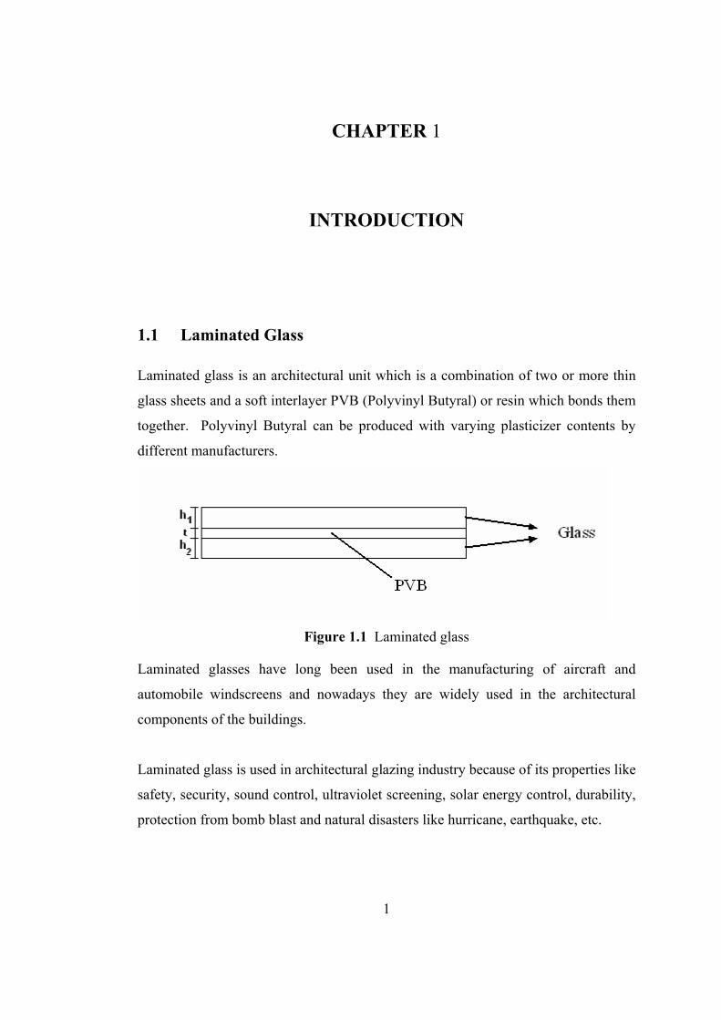
Figure 1.1 Laminated glass 1
Figure 2.1 Laminated Circular Glass Beam with an Interlayer PVB 23
Figure 2.2 Deformed and undeformed sections of laminated glass unit 25
Figure 2.3 Deflection versus load for laminated glass curved beam 32
Figure 2.4 Displacement versus load for laminated glass curved beam for different tolerances
32
Figure 2.5 Displacement versus load for laminated glass straight beam for
different tolerances 32
Figure 2.6 Central deflection values in the fixed supported laminated glass
curved beam 34
Figure 2.7 Maximum stress values in the fixed supported laminated glass
curved beam 35
Figure 2.8 Central deflection values in the monolithic simply supported
curved beam 35
Figure 2.9 Central deflection values in the laminated simply supported
curved beam 36
Figure 2.10 Maximum stress values in the laminated simply supported
curved beam 37
Figure 2.11 Deformed and undeformed shapes of the beam 37
Figure 2.12 A view of meshed finite element model 38
Figure 2.13 Laminated glass beam (Dimensions in mm) 39
Figure 2.14 Comparison of the stresses at center and on the bottom surface
of the laminated glass curved beam. (Strain gage 4) 40
xiv
Figure 2.15 Pictorial presentation of boundary conditions for the simply supported curved beam
41
Figure 2.16 Normalized maximum deflection versus load for simply
supported beam 42
Figure 2.17 Maximum deflection versus load 43
Figure 2.18 Maximum stresses versus load 43
Figure 2.19 Circumferential displacement (u1) of the top glass along the arc
length of the beam 44
Figure 2.20 Circumferential displacement (u2) of the bottom glass along the
arc length of the beam 44
Figure 2.21 Radial deflections for different load values 45
Figure 2.22 Deflections along the arc length of simply supported beam at
load P=2 kN 45
Figure 2.23 Variation of shear stress along the arc length of the beam 46
Figure 2.24 Membrane and bending stresses for the top surface of the top
ply 47
Figure 2.25 Membrane and bending stresses for the bottom surface of the
top ply 47
Figure 2.26 Membrane and bending stresses for the top surface of the
bottom ply 48
Figure 2.27 Membrane and bending stresses for the bottom surface of the
bottom ply 48
Figure 2.28 Stress on bottom surface of the top glass along the arc length of
the simply supported beam 49
Figure 2.29 Stress on top surface of the top glass along the arc length of the
simply supported beam 49
Figure 2.30 Stress on bottom surface of the bottom glass along the arc
length of the simply supported beam 50
xv
Figure 2.31 Stress on top surface of the bottom glass along the arc length of the simply supported beam
50
Figure 2.32 Maximum stresses versus load of the laminated glass 51
Figure 2.33 Stress on the top surface along the arc length of the simply
supported beam at load P=2 kN 52
Figure 2.34 Stress on the bottom surface along the arc length of the simply
supported beam at load P=2kN 52
Figure 2.35 Variation of strength factor of simply supported curved beam 53
Figure 2.36 Pictorial presentation of boundary conditions for the fixed
supported curved beam 54
Figure 2.37 Normalized maximum deflection versus load for fixed
supported beam 55
Figure 2.38 Maximum deflections versus load 56
Figure 2.39 Maximum stress versus load 56
Figure 2.40 Circumferential displacement (u1)of the top glass along the arc
length of the beam 57
Figure 2.41 Circumferential displacement (u2) of the bottom glass along the
arc length of the beam 57
Figure 2.42 Radial deflection for different load values 58
Figure 2.43 Comparison of deflections along the arc length of the fixed
supported beam at load P=2 kN 58
Figure 2.44 Variation of shear stress along the arc length of the beam 59
Figure 2.45 Stress on the bottom surface of the bottom glass along the arc
length of the fixed supported beam 60
Figure 2.46 Stress on the top surface of the bottom glass along the arc
length of the fixed supported beam 60
Figure 2.47 Stress on the bottom surface of the top glass along the arc
length of the fixed supported beam 61
xvi
Figure 2.48 Stress on the top surface of the top glass along the arc length of the fixed supported beam
61
Figure 2.49 Maximum stresses versus load of the laminated glass 62
Figure 2.50 Stress on the top surface along the arc length of fixed supported
beam at load P=2 kN 62
Figure 2.51 Stress on the bottom surface along the arc length of the fixed
supported beam at load P=2kN 62
Figure 2.52 Variation of strength factor with load in a curved beam 63
Figure 2.53 Pictorial presentation of boundary conditions for fixed and
simply supported curved beam 64
Figure 2.54 Maximum deflection versus load for fixed and simply
supported beam 64
Figure 2.55 Maximum stress versus load for fixed and simply supported
beam 65
Figure 2.56 Radial deflections along the beam fixed at one end and simply
supported at the other end for different load values 65
Figure 2.57 Circumferential deflection (u1) of the top glass along the arc
length of the beam 66
Figure 2.58 Circumferential deflection (u2) of the bottom glass along the
arc length of the beam 66
Figure 2.59 Stress on the top surface of top glass along the arc length of the
fixed at one end and simply supported at the other end beam 67
Figure 2.60 Stress on the bottom surface of top glass along the arc length
of the fixed at one end and simple supported at the other end beam
67
Figure 2.61 Stress on the top surface of bottom glass along the arc length of
the fixed at one end and simple supported at the other end beam 68
Figure 2.62 Stress on the bottom surface of bottom glass along the arc
length of the fixed at one end and simple supported at the other end beam
68
xvii
Figure 2.63 Variation of strength factor with load of the laminated curved beam fixed at one end and simply supported at the other end
69
Figure 2.64 Comparison of maximum displacements for different boundary
conditions 69
Figure 2.65 Comparison of maximum stresses for different boundary
conditions 70
Figure 2.66 Comparison of radial deflections along the arc length of the
beam 70
Figure 2.67 Comparison of maximum stresses on the top surface along the
arclength of the beam 71
Figure 2.68 Comparison of maximum stresses on the bottom surface along
the arc length of the beam 71
Figure 2.69 Comparison of strength factor 71
Figure 3.1 Laminated glass cylindrical shell 77
Figure 3.2 Pictorial presentation of boundary conditions for the fixed
supported laminated cylindrical glass shell 87
Figure 3.3 Comparison of central deflection values for monolithic case 104
Figure 3.4 Comparison of central deflection values for the laminated
cylindrical glass shell 106
Figure 3.5 Comparison of the stress values for the laminated cylindrical
glass shell 106
Figure 3.6 A view of contours of radial deflection obtained from
ABAQUS 107
Figure 3.7 Normalized maximum deflection versus load for clamped
cylindrical shell 108
Figure 3.8 Stress versus load for clamped cylindrical shell 109
Figure 3.9 Maximum deflection versus load 110
Figure 3.10 Maximum stress versus load 110
xviii
Figure 3.11 Circumferential displacement of the top glass unit along the center line at y=0
111
Figure 3.12 Circumferential displacement of the bottom glass unit along the
centerline at y=0 111
Figure 3.13 Axial displacement of the top glass unit along the center line at
θ=0 112
Figure 3.14 Axial displacement of the bottom glass unit along the center
line at θ=0 113
Figure 3.15 Radial deflection of the unit along the the centerline at y=0 113
Figure 3.16 Radial deflection of the shell along the diagonal 114
Figure 3.17 Circumferential displacement of the top glass shell along the
diagonal 114
Figure 3.18 Circumferential displacement of the bottom glass shell along
the diagonal 115
Figure 3.19 Axial displacement of the top glass shell along the diagonal 115
Figure 3.20 Axial displacement of the bottom glass shell along the diagonal 115
Figure 3.21 Maximum stress on the top surface of the top glass along the
center line at y=0 116
Figure 3.22 Minimum stress on the top surface of the top glass along the
center line at y=0 117
Figure 3.23 Maximum stress on the bottom surface of the bottom glass
along the center line at y=0 117
Figure 3.24 Minimum stress on the bottom surface of the bottom glass
along the center line at y=0 117
Figure 3.25 Maximum stress on the bottom surface of top shell along the
center line at y=0 118
Figure 3.26 Maximum stress on the top surface of bottom shell along center
line at y=0 119
xix
Figure 3.27 Minimum stress on the bottom surface of top shell along center line at y=0
119
Figure 3.28 Minimum stress on the top surface of bottom shell along center
line at y=0 120
Figure 3.29 Maximum stress on the top surface of the top glass along the
center line at θ=0 121
Figure 3.30 Minimum stress on the top surface of the top glass along the
center line at θ=0 121
Figure 3.31 Maximum stress on the bottom surface of the bottom shell
along the center line at θ=0 122
Figure 3.32 Minimum stress on the bottom surface of the bottom shell along
the center line at θ=0 122
Figure 3.33 Maximum stress on the top surface of the top shell along the
diagonal 122
Figure 3.34 Minimum stress on the top surface of the top shell along the
diagonal 123
Figure 3.35 Maximum stress on the bottom surface of the bottom shell
along the diagonal 123
Figure 3.36 Minimum stress on the bottom surface of the bottom shell along
the diagonal 123
Figure 3.37 Shear stress along θ direction 124
Figure 3.38 Shear stress along y direction 124
Figure 3.39 Contours of radial displacement (mm) for q=10 kPa 125
Figure 3.40 Contours of radial displacement (mm) for q=20 kPa 125
Figure 3.41 Contours of radial displacement (mm) for q=30 kPa 126
Figure 3.42 Contours of radial displacement (mm) for q=40 kPa 126
Figure 3.43 Contours of radial displacement (mm) for q=50 kPa 127
xx
Figure 3.44 Contours of maximum principal stresses (*104 kPa) on the top surface of the top shell for q= 10 kPa
128
Figure 3.45 Contours of maximum principal stresses (*104 kPa) on the top surface of the top shell for q= 30 kPa
128
Figure 3.46 Contours of maximum principal stresses (*104 kPa) on the top surface of the top shell for q= 50 kPa
129
Figure 3.47 Contours of maximum principal stresses (*104 kPa) on the top surface of the top shell for q= 70 kPa
129
Figure 3.48 Contours of maximum principal stresses (*104 kPa) on the top surface of the top shell for q= 90 kPa
130
Figure 3.49 Contours of maximum principal stresses (*104 kPa) on the top surface of the top shell for q= 100 kPa
130
Figure 3.50 Contours of minimum principal stresses (*104 kPa) on the top surface of the top shell for q= 10 kPa
131
Figure 3.51 Contours of minimum principal stresses (*104 kPa) on the top surface of the top shell for q= 30 kPa
131
Figure 3.52 Contours of minimum principal stresses (*104 kPa) on the top surface of the top shell for q= 50 kPa
132
Figure 3.53 Contours of minimum principal stresses (*104 kPa) on the top surface of the top shell for q= 70 kPa
132
Figure 3.54 Contours of minimum principal stresses (*104 kPa) on the top surface of the top shell for q= 90 kPa
133
Figure 3.55 Contours of minimum principal stresses (*104 kPa) on the top surface of the top shell for q= 100 kPa
133
Figure 3.56 Contours of maximum principal stresses (*104 kPa) on the bottom surface of the bottom shell for q= 5 kPa
134
Figure 3.57 Contours of maximum principal stresses (*104 kPa) on the bottom surface of the bottom shell for q= 20 kPa
135
xxi
Figure 3.58 Contours of maximum principal stresses (*104 kPa) on the bottom surface of the bottom shell for q= 30 kPa
135
Figure 3.59 Contours of maximum principal stresses (*104 kPa) on the bottom surface of the bottom shell for q= 50 kPa
136
Figure 3.60 Contours of maximum principal stresses (*104 kPa) on the bottom surface of the bottom shell for q= 70 kPa
136
Figure 3.61 Contours of maximum principal stresses (*104 kPa) on the bottom surface of the bottom shell for q= 90 kPa
137
Figure 3.62 Contours of maximum principal stresses (*104 kPa) on the bottom surface of the bottom shell for q= 100 kPa
137
Figure 3.63 Contours of minimum principal stresses (*104 kPa) on the bottom surface of the bottom shell for q= 10 kPa
138
Figure 3.64 Contours of minimum principal stresses (*104 kPa) on the bottom surface of the bottom shell for q= 30 kPa
139
Figure 3.65 Contours of minimum principal stresses (*104 kPa) on the bottom surface of the bottom shell for q= 50 kPa
139
Figure 3.66 Contours of minimum principal stresses (*104 kPa) on the bottom surface of the bottom shell for q= 70 kPa
140
Figure 3.67 Contours of minimum principal stresses (*104 kPa) on the bottom surface of the bottom shell for q= 90 kPa
140
Figure 3.68 Contours of minimum principal stresses (*104 kPa) on the bottom surface of the bottom shell for q= 100 kPa
141
Figure 3.69 Contours of maximum principal stresses (*104 kPa) on the bottom surface of the top shell for q= 10 kPa
142
Figure 3.70 Contours of maximum principal stresses (*104 kPa) on the bottom surface of the top shell for q= 30 kPa
143
Figure 3.71 Contours of maximum principal stresses (*104 kPa) on the bottom surface of the top shell for q= 50 kPa
143
xxii
Figure 3.72 Contours of maximum principal stresses (*104 kPa) on the bottom surface of the top shell for q= 70 kPa
144
Figure 3.73 Contours of maximum principal stresses (*104 kPa) on the bottom surface of the top shell for q= 90 kPa
144
Figure 3.74 Contours of maximum principal stresses (*104 kPa) on the bottom surface of the top shell for q= 100 kPa
145
Figure 3.75 Contours of maximum principal stresses (*104 kPa) on the top surface of the bottom shell for q= 10 kPa
145
Figure 3.76 Contours of maximum principal stresses (*104 kPa) on the top surface of the bottom shell for q= 20 kPa
146
Figure 3.77 Contours of maximum principal stresses (*104 kPa) on the top surface of the bottom shell for q= 30 kPa
146
Figure 3.78 Contours of maximum principal stresses (*104 kPa) on the top surface of the bottom shell for q= 50 kPa
147
Figure 3.79 Contours of maximum principal stresses (*104 kPa) on the top surface of the bottom shell for q= 70 kPa
147
Figure 3.80 Contours of maximum principal stresses (*104 kPa) on the top surface of the bottom shell for q= 90 kPa
148
Figure 3.81 Contours of maximum principal stresses (*104 kPa) on the top surface of the bottom shell for q= 100 kPa
148
Figure 3.82 Contours of minimum principal stresses (*104 kPa) on the bottom surface of the top shell for q= 10 kPa
149
Figure 3.83 Contours of minimum principal stresses (*104 kPa) on the bottom surface of the top shell for q= 30 kPa
149
Figure 3.84 Contours of minimum principal stresses (*104 kPa) on the bottom surface of the top shell for q= 50 kPa
150
Figure 3.85 Contours of minimum principal stresses (*104 kPa) on the bottom surface of the top shell for q= 70 kPa
150
xxiii
Figure 3.86 Contours of minimum principal stresses (*104 kPa) on the bottom surface of the top shell for q= 90 kPa
151
Figure 3.87 Contours of minimum principal stresses (*104 kPa) on the bottom surface of the top shell for q= 100 kPa
151
Figure 3.88 Contours of minimum principal stresses (*104 kPa) on the top surface of the bottom shell for q= 10 kPa
152
Figure 3.89 Contours of minimum principal stresses (*104 kPa) on the top surface of the bottom shell for q= 30 kPa
152
Figure 3.90 Contours of minimum principal stresses (*104 kPa) on the top surface of the bottom shell for q= 50 kPa
153
Figure 3.91 Contours of minimum principal stresses (*104 kPa) on the top surface of the bottom shell for q= 70 kPa
153
Figure 3.92 Contours of minimum principal stresses (*104 kPa) on the top surface of the bottom shell for q= 90 kPa
154
Figure 3.93 Contours of minimum principal stresses (*104 kPa) on the top surface of the bottom shell for q= 100 kPa
154
Figure 3.94 Strength factor for the fixed supported laminated cylindrical shell
156
Figure 3.95 Comparison of central deflection values for laminated glass
shell 158
Figure 3.96 Comparison of stress values for laminated glass shell 158
Figure 3.97 A view of radial deflection contours obtained from ABAQUS 159
Figure 3.98 Comparison of displacement of the laminated glass subjected to
uniform tension and compressive load 159
Figure 3.99 Maximum deflection versus load 160
Figure 3.100 Maximum stress versus load 160
Figure 3.101 Circumferential displacement of the top glass unit along the
center line at y=0 161
xxiv
Figure 3.102 Circumferential displacement of the bottom glass unit along the center line at y=0
161
Figure 3.103 Axial displacement of the top glass unit along the center line at
θ=0 162
Figure 3.104 Axial displacement of the bottom glass unit along the center
line at θ=0 163
Figure 3.105 Radial deflection of the unit at the center along the center line
at y=0 163
Figure 3.106 Radial deflection of the unit along the diagonal of shell 164
Figure 3.107 Circumferential displacement of the top glass shell along the
diagonal 164
Figure 3.108 Circumferential displacement of the bottom glass shell along
the diagonal 164
Figure 3.109 Axial displacement of the top glass shell along the diagonal 165
Figure 3.110 Axial displacement of the bottom glass shell along the diagonal 165
Figure 3.111 Maximum stress on the top surface of the top glass along the
center line at y=0 166
Figure 3.112 Maximum stress on the bottom surface of the bottom glass
along the center line at y=0 166
Figure 3.113 Minimum stress on the top surface of the top glass along the
center line at y=0 167
Figure 3.114 Minimum stress on the bottom surface of the bottom glass
along the center line at y=0 167
Figure 3.115 Maximum stress at the bottom surface of the top shell along the
center line at y=0 168
Figure 3.116 Maximum stress at the top surface of the bottom shell along the
center line at y=0 169
Figure 3.117 Minimum stress at the bottom surface of the top shell along the
center line at y=0 169
xxv
Figure 3.118 Minimum Stress at the top surface of the bottom shell along the center line at y=0
169
Figure 3.119 Maximum stress on the top surface of the top glass along the
center line at θ=0 170
Figure 3.120 Maximum stress on the bottom surface of the bottom glass
along the center line at θ=0 171
Figure 3.121 Minimum stress on the top surface of the top glass along the
center line at θ=0 171
Figure 3.122 Minimum stress on the bottom surface of the bottom glass
along the center line at θ=0 171
Figure 3.123 Contours of radial displacement (mm) for q=10 kPa 172
Figure 3.124 Contours of radial displacement (mm) for q=20 kPa 173
Figure 3.125 Contours of radial displacement (mm) for q=30 kPa 173
Figure 3.126 Contours of radial displacement (mm) for q=40 kPa 174
Figure 3.127 Contours of radial displacement (mm) for q=50 kPa 174
Figure 3.128 Contours of maximum principal stresses (*104 kPa) on the top
surface of the top shell for q= 10 kPa 175
Figure 3.129 Contours of maximum principal stresses (*104 kPa) on the top surface of the top shell for q= 30 kPa
176
Figure 3.130 Contours of maximum principal stresses (*104 kPa) on the top surface of the top shell for q= 40 kPa
176
Figure 3.131 Contours of maximum principal stresses (*104 kPa) on the top surface of the top shell for q= 50 kPa
177
Figure 3.132 Contours of maximum principal stresses (*104 kPa) on the top surface of the top shell for q= 70 kPa
177
Figure 3.133 Contours of maximum principal stresses (*104 kPa) on the top surface of the top shell for q= 90 kPa
178
xxvi
Figure 3.134 Contours of maximum principal stresses (*104 kPa) on the top surface of the top shell for q= 100 kPa
178
Figure 3.135 Contours of maximum principal stresses (*104 kPa) on the
bottom surface of the bottom shell for q= 10 kPa 179
Figure 3.136 Contours of maximum principal stresses (*104 kPa) on the
bottom surface of the bottom shell for q= 30 kPa 179
Figure 3.137 Contours of maximum principal stresses (*104 kPa) on the
bottom surface of the bottom shell for q= 40 kPa 180
Figure 3.138 Contours of maximum principal stresses (*104 kPa) on the
bottom surface of the bottom shell for q= 50 kPa 180
Figure 3.139 Contours of maximum principal stresses (*104 kPa) on the
bottom surface of the bottom shell for q= 70 kPa 181
Figure 3.140 Contours of maximum principal stresses (*104 kPa) on the
bottom surface of the bottom shell for q= 90 kPa 181
Figure 3.141 Contours of maximum principal stresses (*104 kPa) on the
bottom surface of the bottom shell for q= 100 kPa 182
Figure 3.142 Contours of minimum principal stresses (*104 kPa) on the top
surface of the top shell for q= 10 kPa 182
Figure 3.143 Contours of minimum principal stresses (*104 kPa) on the top
surface of the top shell for q= 30 kPa 183
Figure 3.144 Contours of minimum principal stresses (*104 kPa) on the top
surface of the top shell for q= 40 kPa 183
Figure 3.145 Contours of minimum principal stresses (*104 kPa) on the top
surface of the top shell for q= 50 kPa 184
Figure 3.146 Contours of minimum principal stresses (*104 kPa) on the top
surface of the top shell for q= 70 kPa 184
Figure 3.147 Contours of minimum principal stresses (*104 kPa) on the top
surface of the top shell for q= 90 kPa 185
Figure 3.148 Contours of minimum principal stresses (*104 kPa) on the top surface of the top shell for q= 100 kPa
185
xxvii
Figure 3.149 Contours of minimum principal stresses (*104 kPa) on the bottom surface of the bottom shell for q= 10 kPa
186
Figure 3.150 Contours of minimum principal stresses (*104 kPa) on the bottom surface of the bottom shell for q= 30 kPa
186
Figure 3.151 Contours of minimum principal stresses (*104 kPa) on the bottom surface of the bottom shell for q= 40 kPa
187
Figure 3.152 Contours of minimum principal stresses (*104 kPa) on the bottom surface of the bottom shell for q= 50 kPa
187
Figure 3.153 Contours of minimum principal stresses (*104 kPa) on the bottom surface of the bottom shell for q= 70 kPa
188
Figure 3.154 Contours of minimum principal stresses (*104 kPa) on the bottom surface of the bottom shell for q= 90 kPa
188
Figure 3.155 Contours of minimum principal stresses (*104 kPa) on the bottom surface of the bottom shell for q= 100 kPa
189
Figure 3.156 Pictorial presentation of boundary conditions for the hinged supported laminated cylindrical glass shell
190
Figure 3.157 Central deflection values for hinged cylindrical shell 199
Figure 3.158 Central stress values for hinged cylindrical shell 199
Figure 3.159 A view of radial deflection contour for hinged supported shell 200
Figure 3.160 Normalized maximum deflection versus load for hinged
supported shell 201
Figure 3.161 Stress versus load for hinged supported shell 201
Figure 3.162 Maximum deflection versus load 202
Figure 3.163 Maximum stress versus load 202
Figure 3.164 Circumferential displacement of the top glass unit along the
center line at y=0 203
Figure 3.165 Circumferential displacement of the bottom glass unit along the
center line at y=0 203
xxviii
Figure 3.166 Radial deflection along the center line at y=0 204
Figure 3.167 Axial displacement of the top glass along the center line at θ=0 204
Figure 3.168 Axial displacement of the top glass unit at the center along the center line at θ=0
205
Figure 3.169 Radial deflection along the diagonal 205
Figure 3.170 Circumferential displacement of the top glass shell along the
diagonal 206
Figure 3.171 Circumferential displacement of the bottom glass shell along
the diagonal 206
Figure 3.172 Axial displacement of the top glass shell along the diagonal 206
Figure 3.173 Axial displacement of the bottom glass shell along the diagonal 207
Figure 3.174 Maximum stress at the top surface of the top glass along the θ
direction of hinged supported shell 208
Figure 3.175 Minimum stress at the top surface of the top glass along the θ
direction of hinged supported shell 208
Figure 3.176 Maximum stress at the bottom surface of the bottom glass along
the θ direction of hinged supported shell 208
Figure 3.177 Minimum stress at the bottom surface of the bottom glass
along the θ direction of hinged supported shell 209
Figure 3.178 Maximum stress at the bottom surface of the top glass shell
along the centerline at y=0 210
Figure 3.179 Minimum stress at the bottom surface of the top glass shell
along the centerline at y=0 210
Figure 3.180 Maximum stress at the top surface of the bottom glass shell
along the centerline at y=0 210
Figure 3.181 Minimum stress at the top surface of the bottom glass shell along the centerline at y=0
211
Figure 3.182 Maximum stress at the top surface of the top glass along the
center line at θ=0 212
xxix
Figure 3.183 Minimum stress at the top surface of the top glass along the center line at θ=0
212
Figure 3.184 Maximum stress at the bottom surface of the bottom glass along
the center line at θ=0 212
Figure 3.185 Minimum stress at the bottom surface of the bottom glass along
the center line at θ=0 213
Figure 3.186 Maximum stress at the top surface of the top glass shell along
the diagonal 213
Figure 3.187 Minimum stress at the top surface of the top glass shell along
the diagonal 213
Figure 3.188 Maximum stress at the bottom surface of the bottom glass shell
along the diagonal 214
Figure 3.189 Minimum stress at the bottom surface of bottom glass shell
along the diagonal 214
Figure 3.190 Shear stress of the interlayer along the center line at y=0 215
Figure 3.191 Shear stress of the interlayer along along the center line at θ=0 215
Figure 3.192 Membrane stress along the center line at y=0 for 10 kPa 216
Figure 3.193 Bending stress along the center line at y=0 for 10 kPa 216
Figure 3.194 Membrane stress along the center line at θ=0 for 10 kPa 216
Figure 3.195 Bending stress along the center line at θ=0 for 10 kPa 217
Figure 3.196 Strength factor versus load for hinged supported shell 217
Figure 3.197 Contours of radial displacement (mm) for q=10 kPa 218
Figure 3.198 Contours of d radial displacement (mm) for q=20 kPa 219
Figure 3.199 Contours of radial displacement (mm) for q=30 kPa 219
Figure 3.200 Contours of radial displacement (mm) for q=40 kPa 220
Figure 3.201 Contours of radial displacement (mm) for q=50 kPa 220
xxx
Figure 3.202 Contours of maximum principal stresses (*104 kPa) on the top surface of the top shell for q= 10 kPa
221
Figure 3.203 Contours of maximum principal stresses (*104 kPa) on the top
surface of the top shell for q= 30 kPa 222
Figure 3.204 Contours of maximum principal stresses (*104 kPa) on the top surface of the top shell for q= 40 kPa
222
Figure 3.205 Contours of maximum principal stresses (*104 kPa) on the top surface of the top shell for q= 50 kPa
223
Figure 3.206 Contours of maximum principal stresses (*104 kPa) on the top surface of the top shell for q= 70 kPa
223
Figure 3.207 Contours of maximum principal stresses (*104 kPa) on the top surface of the top shell for q= 90 kPa
224
Figure 3.208 Contours of maximum principal stresses (*104 kPa) on the top surface of the top shell for q= 100 kPa
224
Figure 3.209 Contours of maximum principal stresses (*104 kPa) on the bottom surface of the bottom shell for q= 10 kPa
225
Figure 3.210 Contours of maximum principal stresses (*104 kPa) on the bottom surface of the bottom shell for q= 30 kPa
225
Figure 3.211 Contours of maximum principal stresses (*104 kPa) on the bottom surface of the bottom shell for q= 40 kPa
226
Figure 3.212 Contours of maximum principal stresses (*104 kPa) on the bottom surface of the bottom shell for q= 50 kPa
226
Figure 3.213 Contours of maximum principal stresses (*104 kPa) on the bottom surface of the bottom shell for q= 70 kPa
227
Figure 3.214 Contours of maximum principal stresses (*104 kPa) on the bottom surface of the bottom shell for q= 90 kPa
227
Figure 3.215 Contours of maximum principal stresses (*104 kPa) on the bottom surface of the bottom shell for q= 100 kPa
228
Figure 3.216 Contours of minimum principal stresses (*104 kPa) on the top surface of the top shell for q= 10 kPa
228
xxxi
Figure 3.217 Contours of minimum principal stresses (*104 kPa) on the top surface of the top shell for q= 30 kPa
229
Figure 3.218 Contours of minimum principal stresses (*104 kPa) on the top surface of the top shell for q= 40 kPa
229
Figure 3.219 Contours of minimum principal stresses (*104 kPa) on the top surface of the top shell for q= 50 kPa
230
Figure 3.220 Contours of minimum principal stresses (*104 kPa) on the top surface of the top shell for q= 70 kPa
230
Figure 3.221 Contours of minimum principal stresses (*104 kPa) on the top surface of the top shell for q= 90 kPa
231
Figure 3.222 Contours of minimum principal stresses (*104 kPa) on the top surface of the top shell for q= 100 kPa
231
Figure 3.223 Contours of minimum principal stresses (*104 kPa) on the bottom surface of the bottom shell for q= 10 kPa
232
Figure 3.224 Contours of minimum principal stresses (*104 kPa) on the bottom surface of the bottom shell for q= 30 kPa
232
Figure 3.225 Contours of minimum principal stresses (*104 kPa) on the bottom surface of the bottom shell for q= 40 kPa
233
Figure 3.226 Contours of minimum principal stresses (*104 kPa) on the bottom surface of the bottom shell for q= 50 kPa
233
Figure 3.227 Contours of minimum principal stresses (*104 kPa) on the bottom surface of the bottom shell for q= 70 kPa
234
Figure 3.228 Contours of minimum principal stresses (*104 kPa) on the bottom surface of the bottom shell for q= 90 kPa
234
Figure 3.229 Contours of minimum principal stresses (*104 kPa) on the bottom surface of the bottom shell for q= 100 kPa
235
xxxii
LIST OF TABLES
TABLES Table 2.1 Physical properties of laminated glass curved beam 31
Table 2.2 Comparison of results for the fixed supported laminated
curved beam
34
Table 2.3 Comparison of results for the simply supported laminated
curved beam
36
Table 2.4 Physical properties of laminated glass curved beam 39
Table 2.5 Comparison of central maximum stresses for experimental
and mathematical model results
40
Table 3.1 Comparison of deflections for the monolithic cylindrical
shell
101
Table 3.2 Physical properties of laminated glass shell unit 105
Table 3.3 Comparison of the results for the fixed supported laminated
cylindrical shell
105
Table 3.4 Strength Factor values in building codes 155
Table 3.5 Comparison of the results for the fixed supported laminated
cylindrical shell
157
xxxiii
LIST OF SYMBOLS h1, h2 Thickness of top and bottom glass ply
t Thickness of the interlayer
b Width of beam
h Distance between the midpoints of the top and bottom plies
N1, N2 Cross sectional force at the top and bottom glass ply
u1, u2 Circumferential displacement for the top and bottom ply in the θ
direction
v1, v2 Axial displacement for the top and bottom ply in the y direction
r1, r2 Radius of the top and bottom ply
A1, A2 Cross sectional area of top and bottom glass ply
w Lateral deflection of the top and bottom plies
E Modulus of elasticity of glass
G Shear modulus of interlayer
θ, r polar coordinates
P Point load applied at the middle of beam
q Uniformly distributed load applied over the length of beam
U Total strain energy
V Potential energy of applied loads
Total potential energy of the system
I1, I2 Cross sectional moment of inertia of the top ply
I Cross sectional moment of inertia of the laminated glass section

xxxiv
ı Shear strain in the interlayer for curved beam
θr, γyr Shear strain in the interlayer
Shear stress in the interlayer
U im Membrane strain energy for the top and bottom ply
U ib Bending strain energy for the top and bottom ply
U Shear strain energy for the interlayer
ir
iyr U,U Shear strain energy of the interlayer in the radial and circumferential
directions, respectively
yy ,, Bending strains
yy ,, Membrane strains
Ω Load potential function
Poisson ratio of the interlayer
im Membrane strain energy for the top and bottom ply
ib Bending strain energy for the top and bottom ply
top-top Top surface of the top glass top-bot Bottom surface of the top glass bot-top Top surface of the bottom glass bot-bot Bottom surface of the bottom glass
1
CHAPTER 1
INTRODUCTION
1.1 Laminated Glass Laminated glass is an architectural unit which is a combination of two or more thin
glass sheets and a soft interlayer PVB (Polyvinyl Butyral) or resin which bonds them
together. Polyvinyl Butyral can be produced with varying plasticizer contents by
different manufacturers.
Figure 1.1 Laminated glass
Laminated glasses have long been used in the manufacturing of aircraft and
automobile windscreens and nowadays they are widely used in the architectural
components of the buildings.
Laminated glass is used in architectural glazing industry because of its properties like
safety, security, sound control, ultraviolet screening, solar energy control, durability,
protection from bomb blast and natural disasters like hurricane, earthquake, etc.
2
Laminated glass can help to provide protection from injury, and prevents property
damage from man made and natural disasters by keeping the glass intact within the
frame. When laminated glass is broken, the polyvinyl butyral interlayer keeps the
glass shards together. The interlayer is also advantageous in other respects. Because
of shear damping performance of the PVB, laminated glass is an effective sound
control product. The ability of interlayer to reflect and/or absorb and re-radiate much
of the solar UV radiation, solar control can also be accomplished.
Laminated glass has some disadvantages: it has relatively low bending strength
compared with monolithic glass of the same overall thickness due to the presence of
the plastic interlayer.
Laminated glass units are used in architectural glazing products such as overhead
glazing, safety glazing and insulating glass because of their resistance to a wide
range of loading and environmental conditions. Laminated glass units have the
advantage of withstanding blast pressures, high wind pressures or missile impact
rather than ordinary glass units such as tempered, annealed or heat-strengthened
laminated glass.
Behavior of laminated glass unit is highly complicated because of two different types
of materials, glass and PVB. The modulus of elasticity of glass about 104 times
greater than the elasticity modulus of polyvinyl butyral and laminated glass unit is
very thin, and can easily show large displacement. Therefore, the equilibrium
equations governing their behavior are based on large deflection theory.
Glass unit used as a structural member could be layered, laminated or monolithic.
Layered glass consists of two glass sheets with no friction between them. Stress
distribution of each ply is symmetric with respect to their individual neutral axis. The
glass sheets share the load equally. ‘Plane sections before deformation remain plane
after deformation’ assumption is not valid for layered glass units because centers of
curvature of two plies are different.
3
Monolithic glass consists of one glass sheet. Stress distribution of monolithic glasses
is symmetric around the neutral axis of the glass unit. Because of single center of
curvature, ‘plane sections remain plane’ assumption is valid for monolithic glass
units.
Laminated glass consists of two or more glass sheets connected with an interlayer.
Stress distribution in the cross section of laminated glass is formed as constant
coupling stress of interlayer and the two triangular stress distribution of a layered
glass, which is symmetrical about the neutral axes of each ply. The size of coupling
stress depends on the shear modulus of the interlayer. While coupling stress is
compressive at the top ply, it is tensile at the bottom ply when pressure is applied
towards top ply.
1.2 Previous Research In literature, there are many studies concerned with behavior of laminated glass unit.
A brief summary of the studies is listed below.
1.2.1 Hooper’s Analytical and Experimental Studies
Hooper (1973) conducted the first study about laminated glass beams. In his study, a
mathematical model for the bending of laminated glass beams under four point
loading was derived. The relevant differential equation in terms of applied bending
moment and the axial force in one of the plies were solved using Laplace transform.
Hooper plotted three influence factors K1, K2 and K3 respectively proportional to the
axial force in one of the plies, shear strain in the interlayer and central deflection. He
noted that shear modulus of PVB can be written as a function of time which
approaches zero as time increases, since PVB is a viscoelastic material.
Hooper carried out two types of experiments. At first, tests on laminated glass beam
with soft and hard PVB interlayer under short and long loading durations was
conducted. For short-term loading tests, he bonded strain gages with thin lead wires
to inner and outer glass sheets of laminated glass beam. Then he placed the plastic
4
interlayer between the gaged glass layers and laminated them. He loaded the beams
via universal testing machine at an ambient temperature of o21 C. Gage readings
were taken at several loads. Short-term loading tests took about 3 minutes. Bending
stresses across the laminated glass section and central deflections were obtained. The
changes in shear modulus versus temperature were plotted for soft and hard
interlayer cases.
While load deformation curves were linear and creep deformation was negligible for
beams containing a soft interlayer they were slightly nonlinear and creep deformation
occurred for beams containing a hard interlayer. Results of strain gage readings were
in good agreement with the results of computed strains. Hooper found that shear
strain of the unit was increasing as the interlayer thickness was decreasing. Another
phenomenon observed was the modulus of hard interlayer being ten times higher
than that of soft interlayer.
In addition to above experiments Hooper also conducted creep experiments. In creep
experiments, the applied loads were in the form of dead weights and located at the
quarter points of small laminated glass beams at various temperatures. The
experiment duration was 80 days and measurements of central deflection and
ambient temperature were taken at intervals throughout this period. As results of
creep experiments Hooper plotted shear modulus- temperature graphs and he noted
that the severe degradation of shear modulus of soft interlayer began between 10-20
degrees Celsius whereas it began between 30-40 degrees Celsius for hard interlayer.
Hooper concluded that response of architectural laminated glass unit subjected to
sustained loading for long-term was the same for all types of PVB interlayer. If a
short-term load was applied to the already loaded section, then the stress field could
be calculated by using the combination of sustained and transient loading stresses.
Shear modulus of the soft and hard interlayer at different temperatures were
calculated and shear modulus-temperature graphs were plotted.
The results Hooper (1973) deduced from these studies were that bending resistance
of laminated glasses principally depend upon the thickness and shear modulus of the
interlayer. Creep deformation took place within the plastic interlayer if the applied
loads were sustained except at relatively low temperatures, which allowed the glass
5
layers to deflect as layered glass. But laminated glass would respond as a composite
member having an interlayer shear modulus appropriate to its temperature if it was
undergoing sustained loading.
Hooper advised that for the structural design, architectural laminates, which were
subjected to sustained loads like snow or self-weight loading, should be considered
as layered glass. For short term loading like wind loading, glass bending stresses
might be estimated on the basis of interlayer shear modulus corresponding to the
maximum temperature at which such loading was likely to occur, remembering that
solar radiation might well raise the temperature of glazed laminate to well above that
of surrounding atmosphere. If laminates were subjected to both sustained and
transient loading, the resulting stresses might be calculated by superposition method.
1.2.2 Mathematical Model Developed by Vallabhan
Vallabhan et al. (1983) determined that Von Karman plate theory assumptions were
acceptable for the nonlinear behavior of thin glass plates. Boundary conditions were
prescribed as simply supported. A computer model was developed by Vallabhan et
al. to analyze the nonlinear behavior of monolithic glass plates using finite difference
method. They compared nonlinear behavior of monolithic and layered glass using
the finite difference solution incorporating Von Karman plate theory.
Vallabhan et al. (1987) developed a nonlinear model for two plates placed without an
interlayer to determine the limits of laminated glass units.
Strength factor of glass unit/plate geometries for a wide range of pressures were
considered by them. Nonlinear theory of thin rectangular plates was used for strength
factor analysis. The ratio of maximum principal tensile stress in monolithic glass
system to the maximum principal tensile stress in layered glass system was defined
as the strength factor.
In analysis, they used nondimensional parameters of load, deflection, stress and
aspect ratio. They found that strength factor began to increase nonlinearly, starting
from the linear value of 0.5 to approach and exceed 1, when the pressure increased.
6
In 1993 Vallabhan et al. developed a new mathematical model for the nonlinear
analysis of laminated glass units using the principle of minimum potential energy
and variational calculus. Because of symmetry with respect to x and y axes only a
quarter of plate was considered. Five nonlinear governing differential equations and
boundary conditions were obtained via variational and energy methods. Von Karman
nonlinear plate theory was used for modelling the glass plates. The glass plies were
assumed to have both bending and membrane strain energies while the interlayer has
only shear strain energy. Finite difference method was used to solve the nonlinear
differential equations. All the nonlinear terms were collected on the right hand side
of the differential equation so the left hand side was obtained as linear. To verify the
results obtained from the mathematical model, detailed full-scale exp
eriments were conducted in the Glass Research and Testing Laboratory at Texas
Tech University. They conducted a series of tests on a special laminated unit size
(152.4152.4 cm.). The thicknesses of glass plies and interlayer are 0.47625 cm. and
0.1524 cm., respectively. To provide simply supported boundary conditions they
used round teflon fasteners. The results of mathematical model and experiments were
quite close.
Asik and Vallabhan (1995) studied the convergence of nonlinear plate solutions.
They solved nonlinear plate equations by using two methods. For both of the
methods they used classical Von Karman assumptions and finite difference method.
In the first method they used (Airy stress function) and w (lateral displacement) of
the plate to convert the plate equations. In the second method the same equations
were converted into displacements (u, v, w) of the middle surface of the plate.
Although the above two methods have the same assumptions, convergence
characteristics of them were different. As a conclusion they observed that both
methods yielded the same solution but first method’s convergence was faster than the
second one. They also observed that second model not only converged slowly but
also could diverge after a particular load. For coarser mesh as the displacement
diverged from the actual path the method stopped even at low pressures. However,
when they made fine mesh they could not observe this behavior.
7
Asik (2003) improved Vallabhan’s et al. model (1993) by using modified strongly
implicit (MSI) procedure to avoid the storage of full matrix that needed large
memory and to provide less calculation time. Minimizing the total potential energy
of the laminated glass unit with respect to five displacement parameters, the in-plane
displacements in x and y directions of the two plates and the common lateral
displacement, five nonlinear partial differential equations were obtained as in the
study of Vallabhan et al. (1993).
To write these governing differential equations in discrete form central finite
difference method was used. The discrete form of these equations was written in
matrix form. While symmetric banded coefficient matrix was obtained for lateral
displacement, full coefficient matrices were obtained for each one of in plane
displacements.
He used variable underrelaxation parameter for lateral displacement w while
overrelaxation factor was used for in plane displacements to overcome the
convergence difficulties and to decrease the number of iterations to reach the
solution.
Asik used modified strongly implicit (MSI) procedure for in-plane displacements.
Instead of full coefficient matrix with 2*(nx+1)2*(ny+1)2 elements, the coefficients of
finite difference equations were stored as vectors with totally 2*5*(nx+1)*(ny+1)
elements.
As a conclusion, he applied special solvers that provide advantage in storage and
computation time for nonlinear governing differential equations of a laminated glass.
The results of his study dictated that nonlinearity have to be considered for the
analysis of the behavior of laminated glass units. He observed that location of
maximum stress started to travel at the center and moved towards the corner of the
plate when the nonlinear terms in governing equations start to be affected under
increasing pressure.
8
1.2.3 Experimental Studies conducted by Behr
Behr et al. conducted a series of experiments in 1985 on layered, monolithic and
laminated glass units, to verify the theoretical model for a laterally loaded, thin plates
developed by Vallabhan and Wang (1983).
The experiments were conducted using laminated glass units having dimensions of
152.4243.84 cm. To obtain uniformly distributed load, air was evacuated from the
chamber using vacuum control. To represent the ideal support conditions in the
theoretical model round teflon beads which permit rotation and in-plane
displacement were used. To evaluate the structural behavior of laminated glass unit
tests were performed at temperatures between 0 C and 77 C. As a result of the
experiments, it is concluded that:
1-Stresses in the layered glass unit were larger near the corner and smaller near the
center than comparable stresses in the monolithic glass plate.
2-The maximum principle tensile stress near the corner of laminated glass unit at
room temperature and below were smaller than theoretically predicted stress in a
monolithic glass.
3-At levels above the room temperature, corner stress in laminated glass increased
when temperature was increasing. On the contrary, maximum principle tensile stress
at the center of laminated glass decreased with increasing temperature.
4-Larger principal stresses in layered and laminated glass unit at 77 C were %50
larger than the largest principal stresses of monolithic glass.
Finally, it was observed that stresses in layered glass were larger near the corner and
smaller near the center than monolithic glass plates. It was also observed that at room
temperature and below maximum principal stresses near the corner of laminated unit
were slightly smaller than the theoretically predicted stresses at the same location in
a monolithic glass plate.
It can be said that at room temperature laminated glass unit behaved like a
monolithic glass plate, whereas at higher temperatures it behaved like a layered glass
unit. So the behavior of laminated glass unit was bounded by these two limiting
9
cases. His test results also verified the accuracy of the Vallabhan’s et al. theoretical
model (1983).
Behr et al. (1986) conducted some experiments to consider laminated glass unit
structural behavior for different interlayer thickness and load durations. They
performed multiphased theoretical and experimental research program to develop
and verify analytical models, which define the behavior of laminated glass units used
in building application. Their research included the analysis of laminated glass unit
for a wide range of geometries, failure criteria definition of glass and the effects of
temperature, load duration, chemical and mechanical abrasion and ultraviolet
radiation to the failure criteria and analyze method.
To consider the effect of the interlayer thickness laminated glass unit with two
interlayer thicknesses 0.0762 cm and 0.1524 cm were tested for simply supported
boundary conditions and uniform lateral pressure.
It was concluded that the glass unit with a thicker interlayer have reduced flexural
stiffness. Interlayer thickness affected magnitude of the maximum stress by less than
%10 while the maximum difference in these two deflections was %5. As a result, it is
concluded that the effect of interlayer thickness on laminated glass unit did not
appear to be significant.
To consider the effect of long duration loading on laminated glass units a 152.4
243.80.71 cm unit was subjected to a lateral pressure of 1.4 kPa for 3500 seconds
or 1 hour. The tests were performed at C22 , C49 and C77 .
As a result of long duration loading tests at different temperatures they concluded
that, for all three test temperatures there was 20 % increase for corner stress, while
maximum lateral deflection at the center of the unit increased by 10 %. Conversely,
principal stresses at the center of laminated glass unit decreased slightly.
Behr et al. (1993) reported the results of theoretical and experimental studies
conducted over a 20-year time period by several researchers. Their objectives were to
review and assess information about the structural behavior of architectural
laminated glass and to provide a compendium of research results. They considered
the major structural characteristics of laminated glass like load deflection behavior,
10
load stress relationships, temperature effects, duration of loading, interlayer thickness
and aspect ratio.
They noted that temperature effect was significant for the behavior of laminated
glass units at 77 oC, but were not significant at room temperatures. Conversely,
Hooper’s test (1973) showed a severe degradation in effective shear modulus of
interlayer below the room temperature. Differences in PVB chemistry and
differences between the experiment procedures could explain the differences
between the results of Hooper and Behr.
They also considered the relationship of surface stress to lateral pressure in the
structural behavior of laminated, layered and monolithic glass. They concluded that
similarities existed between monolithic and laminated glass stresses at room
temperature and below but at elevated temperatures stresses of laminated glass
moved towards layered glass stresses.
The effect of duration of loading on the structural behavior of laminated glass was
considered by Behr et al. While dead loads and snow loads produce long duration
loading, wind loads produce load durations measured in seconds. Hooper (1973)
performed creep tests on small scale laminated glass beams under four point loading
of 49 o C, 25 o C and 14 o C. They observed very small amount of creep over the 80
day loading period and the behavior of laminated glass was nearly layered at 25 o C
while they observed no creep and layered behavior at 49o C. At 14 o C the behavior of
laminated glass unit was completely monolithic and substantial creep was observed
at 80 days load duration. So Hooper concluded that substantial creep was observed at
low temperatures.
Behr (1986) performed full scale creep tests under 1 hour on a laminated glass at
temperatures 22 o C, 49 o C and 77 o C. They made the following observations as a
result of their test:
1. The increase in corner stress was 22 % at 77o C and 49o C while it was 18% at 22o
C.
2. There was a decrease at the center principal stresses of laminated glass unit for all
three test temperatures over the 1 hour loading duration.
11
3. The increase in maximum lateral deflection at the corner of laminated glass unit
was 10% for all three test temperatures over the 1 hour load duration.
The results of Behr’s full scale laminated glass plate tests were different from the
Hooper’s small scale test results. The creep was pronounced for small scale
laminated glass beams. This difference was attributable to the difference in PVB
chemistry.
Behr noted that the impact resistance of laminated glass units increased when the
thickness of PVB interlayer increased.
Hooper (1973) observed a reduction in effective shear modulus of hard PVB as the
result of small scale beam tests. As the interlayer thickness increased from 0.38 mm
to 1.02 mm the shear modulus decreased from 15.2 MPa to 11.7 MPa. They did not
investigate the effect of interlayer thickness for soft PVB interlayer.
Behr et al. (1986) conducted tests on laminated glass unit with interlayer thicknesses
of 0.76 mm and 1.52 mm. They observed small differences in the stress and
deformation responses of the units. Laminated glass unit with 1.52 mm interlayer
thickness had higher stresses and deflections than laminated glass unit with 0.76 mm
interlayer thickness. The differences in maximum stresses were less than 10% while
they were below 5% for deflections.
In order to examine the structural behavior of laminated glass unit with large aspect
ratios, experiments were conducted at 0o C, 23o C and 49o C.
While center deflections of laminated glass beam specimens tested at 0o C were
lower than those in monolithic beams, they were almost equal at 23o C. At 49o C the
central deflections of laminated units were higher than the deflections of monolithic
beams but significantly less than those in layered beams. They sustained the
maximum load for 1 minute and they observed 11%, 18% and 9% increases for the
central deflections of laminated glass beams tested at 49o C, 23o C and 0o C,
respectively.
They observed that at room temperature and below, the stresses in laminated units
were equal to or lower than those in monolithic glass beams; While they were higher
than the stresses of monolithic glass beam at 49o C. Increase of stresses were
observed as 8%, 6% and 4% at 49o C, 23o C and 0o C, respectively when the constant
12
2.8 kPa load was held constant for sixty seconds. It was concluded that even at high
aspect ratios, under short term loading and below room temperature laminated glass
appeared to behave like monolithic glass.
1.2.4 Norville developed a theoretical model
Norville et al. (1999) developed a theoretical model, which explained the behavior of
laminated glass. The model was based on mechanics of materials and indicated that
the interlayer in laminated glass provided an increase in effective section modulus
with respect to monolithic glass beam having the same nominal thickness. The
increase in effective shear modulus resulted in lower flexural stresses and higher
fracture strengths. PVB’s function in laminated glass unit was assumed to maintain
spacing between the glass plies and transferring a fraction of the horizontal shear
force between the glass plies. Effective section modulus for laminated glass under
uniform loading as a function of the fraction of horizontal shear force transferred by
the PVB interlayer could be computed by using this model. The horizontal shear
force transferred by the interlayer between the glass plies was expressed as the
product of a shear force transfer parameter and the horizontal shear force of middle
fiber of monolithic glass beam. The laminated glass beam acted as a layered glass
beam when this parameter was zero. It behaved as a monolithic glass beam when the
parameter was 1.
Norville et al. performed laminated glass beam test to verify measurements of center
deflection reported by Behr (1993). The results were in close agreement and
deflections predicted by this model strongly supported the model’s validity. They
also performed laminated glass lite tests and observed that laminated glass series
with varying thickness, dimension and loading displayed mean fracture stress
ranging from 98% to 230% that of monolithic series of the same dimensions.
As a conclusion, they developed a theoretical model to investigate the behavior of
laminated glass under uniform loading. PVB was assumed to transfer a horizontal
shear force between the glass plies. They observed that, for the laminated glass, to
13
produce equivalent or greater section modulus than monolithic glass, the fraction of
shear force transfer was less than 1, and at 49oC behavior of the laminated glass was
far below the layered glass model. At room temperature, under short duration (<60
sec.) uniform loading, laminated glass constructions indicated lower stresses. In
addition, laminated glass units had equivalent or higher fracture strengths than
monolithic glass units with the same dimensions and thickness.
1.2.5 Van Duser developed a finite element model
Van Duser et al. (1999) presented a three dimensional finite element model based on
large deformation for stress analysis of laminated units. The analysis had capability
to predict the stress generated during biaxial flexure. They solved a laminated glass
subjected to uniform pressure using the commercial finite element model ABAQUS
(1997) to demonstrate the accuracy of their approach. They solved the models tested
by Vallabhan et al. (1993) to be able to compare their results. They also combined
stress analysis with a Weibull statistical probability of failure, to describe the load
bearing capacity of laminates of arbitrary shape and size under specific loading
conditions. As a result of their study they concluded that laminated glass polymer
units behaved in a complex manner due to large difference between stiffness of
materials, nonlinearity, large deflection, polymer viscoelasticity and additional
stiffening effect of polymer thickness. They also observed that stress development
might fall outside of the monolithic and layered limit because of the membrane
stresses of plate. The other finding of their study was that stress development was
influenced by temperature. At higher temperatures and loads principal stresses
shifted systematically towards the corner. They concluded that under almost all
conditions Weibull effective stress was lower for laminated plates than for the
equivalent monolithic one.
14
1.2.6 Minor conducted experiments about failure strength
Minor et al. (1990) conducted some tests to make comparisons between failure
strengths of monolithic and laminated glass units. They selected three sizes of
annealed monolithic glass samples: 152.4243.840.635 cm; 96.52193.040.635
cm and 167.64167.640.635 cm. These samples were used to evaluate the failure
strengths as function of several variables like; temperature, glass type (heat
treatment) and surface conditions. Laminated glass samples were selected as heat
strengthened and fully tempered. To apply uniform pressure to test specimens, an
accumulator was used to evacuate air from vacuum chamber. As a result, failure
strengths of laminated glass and annealed monolithic glass samples were compared.
At room temperature laminated glass strengths and monolithic glass strengths were
found to be equal whereas the strength of laminated glass decreased when
temperature were elevated. It is also observed that fully tempered and heat
strengthened laminated glass samples were 3 or 5 times stronger than annealed
laminated and monolithic glass samples.
1.2.7 Studies about Shell Structures
There are no studies about nonlinear behavior of laminated glass shell structures. But
some of the studies about shell structures are summarized below.
Turkmen (1999) studied cylindrically curved laminated composite panels subjected
to the blast shock wave. He obtained numerical and theoretical results for this
problem and considered the effect of curvature and fiber orientation angle. Love’s
theory for thin elastic shells was used for mathematical modeling. The resulting
equations were solved by using Runga-Kutta method. In addition to the numerical
analysis (Runge–Kutta Method), finite element program ANSYS was used to obtain
results for cylindrically curved shell. The results were compared and a good
agreement was found. Turkmen concluded that the central deflection of the clamped
cylindrical laminated shell decreased and response frequency of the panel increased
while the stiffness of the panel was increasing. Also the effect of damping and
loading conditions considered for this composite panel.
15
Schimmels and Plazatto (1994) analyzed nonlinear geometric behavior of laminated
shell geometry by using orthogonal curvilinear coordinates. They applied
transformation between Cauchy and Lagrangian coordinate system for isotropic and
composite shells. Using nonlinear strain displacement relations and minimum
potential energy theory nonlinear algebraic equations were obtained for
displacements. To solve the nonlinear equations they were converted to linear
equations and finite element method was used to solve these equations.
They verified their model by using the results of Sabir (1972). It is observed that the
fiber rotations became large enough to affect the material transformation matrix
when the shell displacement reached three times of the shell thickness.
Aksogan and Sofiyev (2001) considered the dynamic stability of a laminated
truncated conical shell with variable modulus of elasticity and densities in the
thickness direction subject to a uniform external pressure, which is a power function
of time. Analytical solutions were obtained for the critical dynamic and static loads
and pertinent wave numbers. To verify the results, the critical dynamic loads for a
truncated conical shell with a single layer, found analytically in the present study
were compared with those found experimentally by Sachenkov and Klementev
(1980). They also considered nonlinear free vibration of laminated non- homogenous
orthotropic cylindrical shells. The equations and basic relations were based on the
Donnel-Musthari shell equations. By using Galerkin method frequency of the
cylindrical shell was obtained from Donnel-Musthari shell equations as a function of
shell displacement and compared with the results in literature. It was observed that
the number and ordering of the layers affect the values of vibration frequencies both
in the homogenous and non-homogenous cases.
1.2.8 Studies about curved beam
D. J. Dawe (1974) presented finite element model for the solution of a circular arch
with radius R and thickness t. The strain energy of the system was written in terms of
16
tangential and normal components of displacements. To obtain the differential
equations which govern the behavior of the arch, the first variation of the energy was
used. By solving two differential equations, tangential and radial displacements were
obtained. Five circular arch models, which are given below where numerically
solved. Those models were:
i) Quintic-quintic model with twelve independent coefficients in the expressions of
displacement. Six of them were for normal displacement u and six for tangential
displacement w.
ii) Cubic-quintic model with ten independent coefficients in the expressions of
displacements (6 independent coefficients four u and 4 for w).
iii) Quintic-cubic model with 4 independent coefficients for tangential displacement
and 6 independent coefficients for normal displacement.
iv) Cubic-cubic model with 4 independent coefficients for tangential displacement
and normal displacement.
v) A constant strain, linear curvature element based on the coupled displacement
field.
To apply the described models a computer program which double precision
arithmetic throughout was used to solve arch problems. He obtained the
displacements, moments, force distribution of a deep clamped arc carrying a point
load. As a result of study he improved an independently interpolated model by
increasing the order of assumed displacement from cubic to quintic.
Rajasekaran and Padmanabhan (1989) derived the governing equations for curved
beams by employing large displacement theory. To obtain the governing equations
they ignored shear strains due to shear stress and shear strains in the planes normal to
middle surface. In the solution procedure, the large displacements and the small
strains were also assumed, and the length of the member was much larger than the
depth. To start the derivation they used three-dimensional small strain large
displacement relations in cylindrical coordinate system by ignoring the nonlinear
terms associated with displacement in z direction (w), since it was much smaller
compared to the displacement in x and y directions. They wrote the equilibrium
17
equations and boundary conditions by integrating the principle of virtual
displacement as the product of Kirchhoff stress tensor and Green’s strain tensor.
Palani and Rajasekaran (1992) presented a model for static and stability analysis of
thin walled curved beams made of composites by using straight beam element. In the
study, they used Euler-Lagrange equilibrium equations and the associated boundary
conditions derived by Rajasekaran and Padmanabhan (1989). To derive flexural
stiffness matrix they used straight beam element by employing suitable
transformations. While lateral displacement and angle of twist were represented by
first order Hermitian polynomial, axial displacement was represented by zeroth order
Hermitian polynomial for static analysis. The new curved beam model, which was
obtained by using straight beam, required less computational effort, and the results
were accurate and could be implemented in the programs like SAP. To verify the
model they compared their results obtained for curved beam subjected to uniformly
distributed radial loads with the results of Timoshenko and Gere (1961) and
Rajasekaran and Padmanabhan (1989).
Kang and Yoo (1994) presented a consistent formulation for thin walled curved
beams. They derived equilibrium equations governing the linear, large displacement
and buckling behavior using the principle of minimum potential energy. In their
study, it is assumed that:
1. Cross sections retained their original shapes.
2. The displacements were finite.
3. The shear stresses and strains were negligibly small.
4. The shear stress strains along the middle surface were negligibly
small.
5. The length of beam was much larger than the other dimensions of the
beam.
6. The radius of curvature was large.
To obtain the governing differential equations the total potential energy of the system
was defined as the summation of strain energy and potential energy due to applied
18
loads. By neglecting the nonlinear term of the equations, they obtained the equations
for linear behavior of a curved beam. The governing coupled differential equations of
displacement (i.e. longitudinal, radial and vertical displacement) and boundary
conditions of the curved beam were obtained via the first variation of total potential
energy. In their derivation, the curvature effect was included. Analytical solution to
the coupled equations obtained was not easy: In order to solve the equations an
approximation based on the binomial series was adopted by ignoring the higher order
terms. The derivation was more reliable than the previous derivation because of the
following three advantages: First, they preferred energy method instead of free body
method because free body method involved possibility of omitting some significant
terms. Secondly, their interpretations were appropriate for thin walled curved beam.
Lastly, their approximation was explicit and consistent.
Lin and Heish (2006) developed a closed form analytical solution for in plane
laminated curved beam of variable curvatures. Before their study there were only a
few paper devoted to laminated composite materials. Most of the studies were about
the isotropic beam. To analyze curved beams numerically and analytically,
approximate methods were applied for the displacement field by the previous
researchers. They obtained the set of equations, which were the general solutions of
axial force, shear force, moment, rotation angle and displacement field for laminated
curved beam in terms of angle of tangential slope.
To show the validity of the model they compared the results of their study with the
results of published articles for isotropic material. Also they solved various curved
laminated beams such as cycloid, exponential spiral, catenary, parabola and elliptic
under various loading cases.
1.3 Object and Scope of Thesis
Because of the high difference between the elasticity modulus of glass sheets and
interlayer, the classic assumption that ‘plane section for the whole system before
deformation remains plane after deformation’ is not realistic for laminated glass
19
units. Therefore, the existing theories in the literature cannot be employed for the
analysis of laminated curved glass beam and shell structures.
The aim of the present study is to investigate the behavior of laminated curved glass
beams and cylindrical shells. To develop a more realistic model it is assumed that
plane section before bending remains plane after bending for each individual sheet
and the interlayer translate a certain amount of shear between the glass sheets.
Deflection and stress resultant values, the level of nonlinearity on the bending
behavior and the effect of boundary conditions, strength factor of laminated curved
glass beams and shells are obtained. Mathematical model and computer program are
developed to analyze the nonlinear behavior of curved beams and shells. The model
is based on minimum potential energy principle and variational approach. To verify
the results of developed model nonlinear finite element analyses are performed for
curved beam and shell structures. Besides, results of curved beam experiments
previously conducted by Uzhan (2010) are used to verify the developed model.
Chapter 1, provides an introduction to the thesis and gives information about
laminated glass units and background for the studies of laminated glass unit.
Chapter 2, Laminated curved glass beams are analyzed. The total potential energy of
curved beam is expressed in terms of radial and circumferential displacement.
Minimum potential energy principle and variational approach are used to obtain three
nonlinear governing differential equations and boundary conditions. The equations
are converted into matrix form by using finite difference method. Using iterative
solution technique, the equations are solved. The results are verified by using finite
element method and by comparing with the results obtained from experiments
conducted in Experimental Mechanics Laboratory in the Department of Engineering
Sciences at Middle East Technical University by Uzhan (2010). The results of study
are given in graphs and interpreted in conclusion.
Chapter 3, Laminated glass shell structures are analyzed. The total potential energy
of shell is expressed in terms of radial and circumferential displacement. Minimum
potential energy principle and variational approach are used to obtain the five
nonlinear governing differential equations and boundary conditions. The equations
are converted into matrix form by using finite difference method. Using iterative
20
solution technique, the equations are solved. The results are verified by using finite
element method. The results of the study are given in graphs and interpreted in
conclusion.
Chapter 4, conclusions and recommendations obtained as result of study are given
21
CHAPTER 2
BEHAVIOR OF LAMINATED CURVED GLASS BEAMS
2.1 Introduction to Theory of Curved Beams
It has been quite a time since laminated glasses are in use. First laminated glasses
with flat shapes were used as their production was easy, and design parameters were
available. Nowadays, curved laminated glasses are also used in many modern
buildings. Also curved elements can be used for spring design, electrical machinery
blades, aerospace structures, design of arch bridges and highway constructions.
Curved beams are two dimensional structures which span the spaces. They are used
to support loads from above. Because of the downward pressure, curved beams can
carry much greater load than a straight beam. According to their structural behavior,
curved beams are classified as fixed, hinged, two-hinged or tree-hinged. To satisfy
fixed boundary conditions at the supports rotation is prevented. Fixed ended curved
beams are more suitable for large spans than hinged ended curved beams because of
their greater stiffness.
Because of lack of information about structural behavior of curved beams, they have
not been employed much in practice. A curved beam differs from a straight beam due
to its initial curvature. Because of mathematical complexity, most of the studies are
about the linear behavior rather than the nonlinear behavior of curved beams.
22
Therefore, it is necessary to develop a mathematical model considering large
deflection theory to predict the strength and behavior of curved beams.
In the present study, the behavior of the laminated glass curved beams is investigated
since the curved glass units are being used in modern buildings nowadays and to
author’s knowledge, there is not any significant research on the laminated glass
curved beams. Mathematical model is developed to predict the deflections and
stresses developing in the unit in polar coordinates. Minimum potential energy
principle is used to minimize the total potential energy which is the summation of
the bending and membrane energies in glasses and the energy due to the shear
deformation in the soft interlayer and force potential. Three nonlinear coupled
differential equations are derived through variational principles. Numerical model is
developed to solve the continuous form of the governing equations. Finite difference
method is employed for the discretization of the nonlinear partial differential
equations, and then those equations are solved iteratively. The model is verified by
using the data obtained from the finite element model and using previously done
experimental results by Uzhan [27]. Results are presented by the figures for the
verification of the model and the prediction of the behavior. Moreover, the behavior
of laminated glass beams is presented in comparison to the behavior of the
monolithic and layered glass beams as limiting cases since the design charts are
available only for monolithic glasses.
2.2 Mathematical Modeling
Behavior of the laminated curved beam- shown in Figure 2.1-, which contains two
thin glass sheets and an interlayer PVB placed in between the glass sheets, can be
represented by three nonlinear partial differential equations obtained for three
displacement components. Two of these equations are used to represent
circumferential displacements and the third one is for the radial displacement of the
unit.
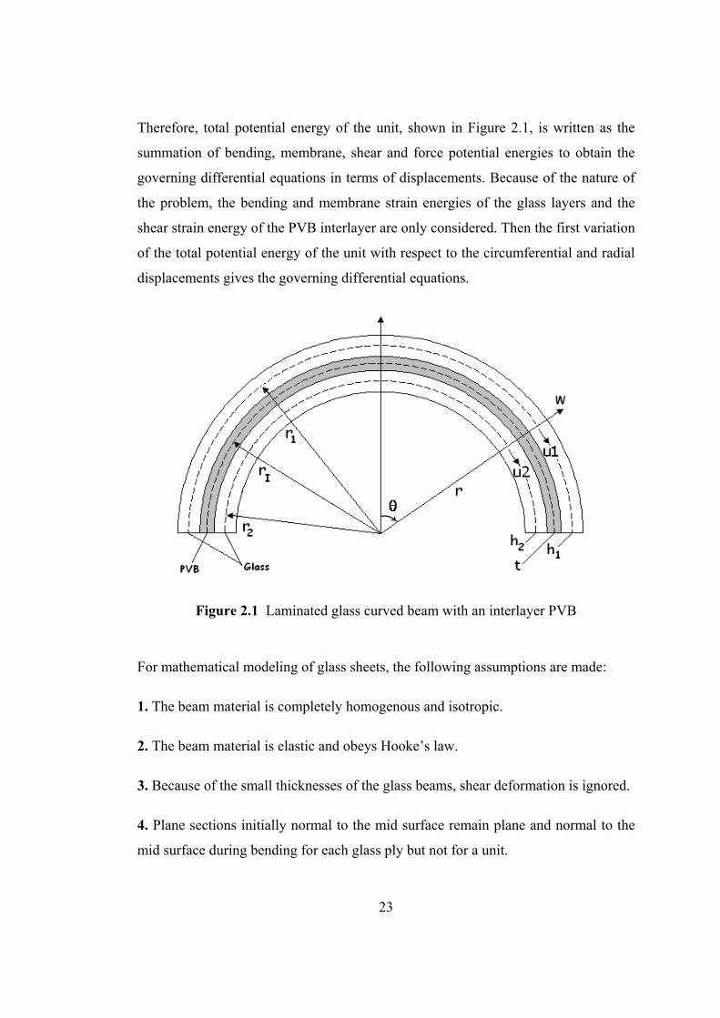
23
Therefore, total potential energy of the unit, shown in Figure 2.1, is written as the
summation of bending, membrane, shear and force potential energies to obtain the
governing differential equations in terms of displacements. Because of the nature of
the problem, the bending and membrane strain energies of the glass layers and the
shear strain energy of the PVB interlayer are only considered. Then the first variation
of the total potential energy of the unit with respect to the circumferential and radial
displacements gives the governing differential equations.
Figure 2.1 Laminated glass curved beam with an interlayer PVB
For mathematical modeling of glass sheets, the following assumptions are made:
1. The beam material is completely homogenous and isotropic.
2. The beam material is elastic and obeys Hooke’s law.
3. Because of the small thicknesses of the glass beams, shear deformation is ignored.
4. Plane sections initially normal to the mid surface remain plane and normal to the
mid surface during bending for each glass ply but not for a unit.
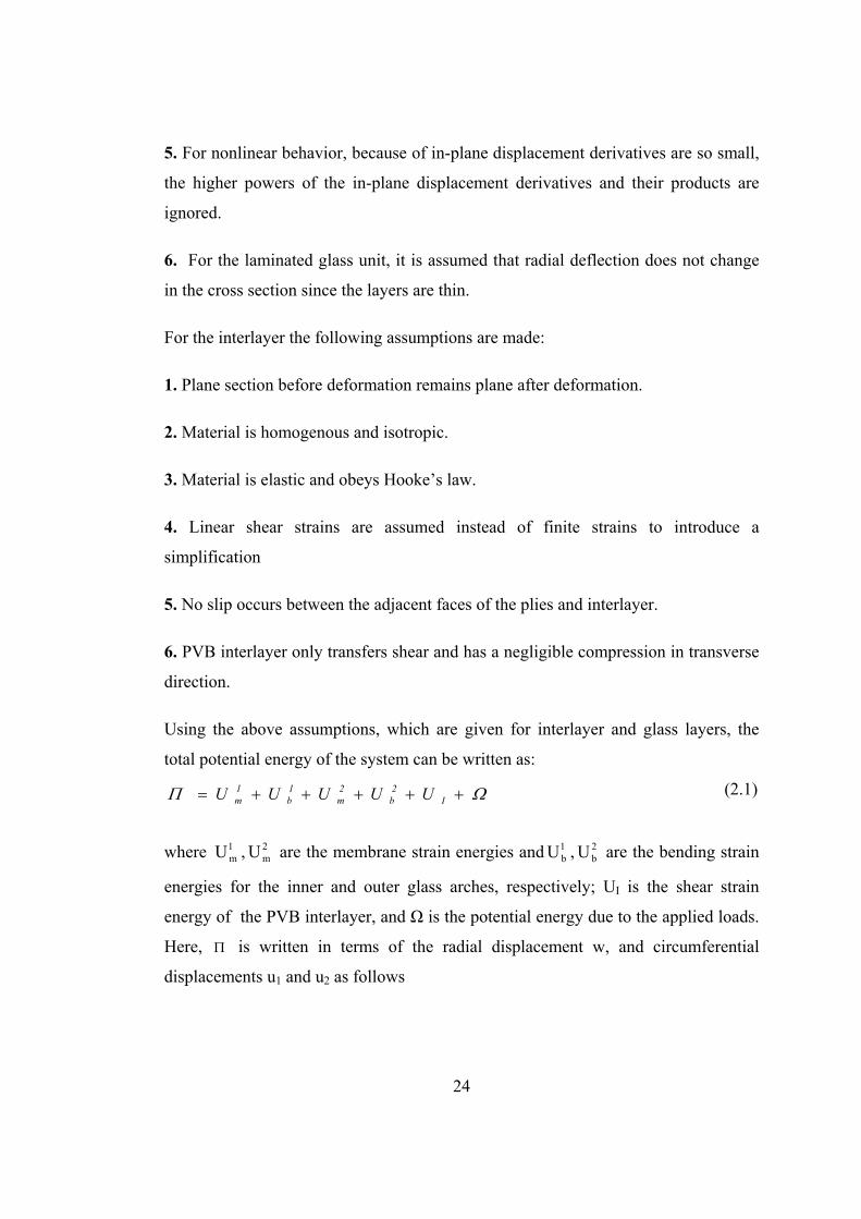
24
5. For nonlinear behavior, because of in-plane displacement derivatives are so small,
the higher powers of the in-plane displacement derivatives and their products are
ignored.
6. For the laminated glass unit, it is assumed that radial deflection does not change
in the cross section since the layers are thin.
For the interlayer the following assumptions are made:
1. Plane section before deformation remains plane after deformation.
2. Material is homogenous and isotropic.
3. Material is elastic and obeys Hooke’s law.
4. Linear shear strains are assumed instead of finite strains to introduce a
simplification
5. No slip occurs between the adjacent faces of the plies and interlayer.
6. PVB interlayer only transfers shear and has a negligible compression in transverse
direction.
Using the above assumptions, which are given for interlayer and glass layers, the
total potential energy of the system can be written as:
(2.1)
where 1mU , 2
mU are the membrane strain energies and 1bU , 2
bU are the bending strain
energies for the inner and outer glass arches, respectively; UI is the shear strain
energy of the PVB interlayer, and Ω is the potential energy due to the applied loads.
Here, is written in terms of the radial displacement w, and circumferential
displacements u1 and u2 as follows
I2
b2m
1b
1m UUUUU
25
(2.2)
where
Shear strain of the unit is obtained from deformed and undeformed geometry as seen
in Figure 2.2.
Figure 2.2 Deformed and undeformed sections of laminated glass unit
Shear strain for the interlayer is:
s
0qwds
VdV2)
I(G
21
2
1i VdV2)i
b(E
21
VdV2)i
m(E
21
2
1
1m r
w
2
1
r
w1u
1
2
22
2m r
w
2
1
r
w2u
22
θθ2b
r
wzε
t
d
dw
r
t
2
h
r
1
2
h
r
12u1u
I
2
2
1
1I
21
1b r
wz
h1
h2
t w
θ-axis
Undeformed Section u2
Deformed Section
u1
y-axis
26
Therefore the total potential energy of the system in extended form is:
(2.3)
Variation of total potential energy with respect to radial displacement, w, and
circumferential displacements, u1 and u2, gives following stationary equations.
01u
02u
0w
Therefore, three nonlinear coupled differential equations and boundary conditions for
a laminated glass curved beam are obtained:
0qrd
d
r
t
2
h
r
1
2
h
r
1Gbr
2N1Nd
dw
r
2N
r
1N
d
d
d
wdEI
d
d
1I
I
2
2
1
1I
212
2
2
(2.4)
0Gbrd
1dNII
(2.5)
0Gbrd
2dNII
(2.6)
s
0V
2
2
2
1
121
2
1i V
22
i21
V
2
2
ii21
qwdsdV)t
d
dwt
2
h
r
1
2
h
r
12u1u
(G
dV)r
wz(EdV)
r
w
2
1
r
wui(E
rI
27
in which
(2.7)
(2.8)
21 III in which 3
1
31
1r12
bhI ,
32
32
2 12r
bhI ;
where N1 and N2 are the outer and inner circumferential forces in glass arches,
respectively. I is the shear strain in the interlayer; G is the shear modulus of
interlayer; E is the elasticity modulus of glass; h1 and h2 are the thicknesses of outer
and inner glass arches; A1 and A2 are the cross section areas of outer and inner glass
arches, respectively; b is the width of the unit; q is a uniformly distributed load; and I
is the moment of inertia of the glass arches.
The governing equations (2.4) to (2.6) in terms of displacements are:
d
2du
d
1du
r
t
2
h
r
1
2
h
r
1
t
Gbr
)1w(r2
w
r
w2u
r
EAw
r
ww
r
w2u
r
EA
)1w(r2
w
r
w1u
r
EAw
r
ww
r
w1u
r
EA
qrw
2
r
t
22
h
r
1
21
h
r
1
tI
Gbr
4d
w4dEI
I
2
2
1
1
I
22
2
22
22
222
2
21
2
11
12
111
1
1I21
(2.9)
d
dw
r
t
2
h
r
1
2
h
r
12u
t
Gbr
)wr
11)(w(
r
EA1u
t
Gbr)1u(
r
EA
I
2
2
1
1
I
11
1I
1
1
(2.10)
)wr2
1
r
w1u(EA1N 2
211
1
)wr2
1
r
w2u(EA2N 2
222
2
28
d
dw
r
t
2
h
r
1
2
h
r
11u
t
Gbr
)wr
11)(w(
r
EA2u
t
Gbr)1u(
r
EA
I
2
2
1
1
I
22
2I
2
2
(2.11)
Boundary equations of curved beam could be obtained as follows:
At 1 and 2 (at supports of curved unit) for Equation (2.4)
~V
d
dw
r
t
2
h
r
1
2
h
r
12u1u
r
t
2
h
r
1
2
h
r
1
t
Gbr
d
dw2N1N
2d
w2dEI
d
d
I
2
2
1
1I
2
2
1
1
I
or radial deflection w is prescribed,
~M
2d
w2dEI
or
d
dw is prescribed,
for Eqs. (2.5) and (2.6)
~
1Nr2
w
r
w1u
r
EA2
1
2
11
1
or 1u is prescribed and
~2N
r2
w
r
w2u
r
EA2
2
2
22
2
or 2u is prescribed;
where ~V is the applied shear force,
~M is the applied moment and
~1N ,
~2N are the
applied axial forces for outer and inner glass arches, respectively.
For a simply supported laminated curved glass beam without applied forces at the
ends, as a special case, boundary conditions take the following form:
at 1 and 2 (at the supports): w = 0 and 0d
wd2
2
01u and 02u
29
For a fixed supported laminated curved glass beam without applied forces at the
ends, as a special case, boundary conditions take the following form:
at 1 and 2 (at the supports): w = 0 and 0d
dw
01u and 02u
Analytic solution of three governing nonlinear differential equations (2.9)-(2.11) is
difficult. Therefore, the numerical Finite Difference Method (FDM) is used to solve
the governing equations (2.9)-(2.11). The solution procedure given by Asik [24] is
modified for a curved beam. The nonlinear differential equations are converted into
algebraic equations by using central finite difference method and written in matrix
form. All nonlinear terms in the equations are placed on the right hand side. Then,
governing equations become:
RwA (2.12)
where A is a qui-diagonal matrix, and only the elements belonging to five diagonals
are stored as vectors. The right hand side vector, R includes applied load and other
terms are calculated at every discrete point on the right hand side of Equation (2.9).
Iterative procedure is employed since the equations are coupled and nonlinear. The
equations are modified at the boundaries of the unit. Applied load is considered in
small increments for convergence, where:
w = the radial displacement vector,
[A]=coefficient matrice for radial displacement.
For the radial deflection, the finite difference mesh size is chosen to be , n is the
number of subdivisions in the θ directions. In order to reduce the total number of
equations the radial deflection values at the fixed supported edges which are zero, are
not incorporated. Central finite difference expression of the field equation for the
radial deflection in the domain is:
iRHS
2iEw
1iDw
iCw
1iBw
2iAw
, (2.14)
for i=1, 2,…, n-1.
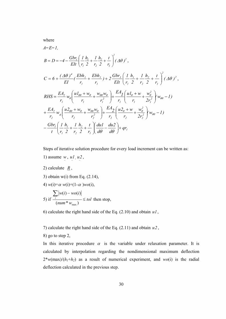
30
where
A=E=1,
2
2
I
2
2
1
1
I )(r
t
2
h
r
1
2
h
r
1
EIt
Gbr4DB
,
2
2
I
2
2
1
1
I
1
1
1
14
)(r
t
2
h
r
1
2
h
r
1
EIt
Gbr2)
r
Ebh
r
Ebh(
EI
)(6C
,
1I
2
2
1
1
I
22
2
222
222
2
21
2
112
111
2
qrd
2du
d
1du
r
t
2
h
r
1
2
h
r
1
t
Gbr
)1w(r2
w
r
w2u
r2
EA
r
ww
r
w2uw
r
EA
)1w(r2
w
r
w1u
r1
EA
r
ww
r
w1uw
r
EARHS
Steps of iterative solution procedure for every load increment can be written as:
1) assume w ,
1u ,
2u ,
2) calculate R ,
3) obtain w(i) from Eq. (2.14),
4) w(i)= w(i)+(1- )wo(i),
5) if tolwnum
iwoiwi
)*(
)()(
max
then stop,
6) calculate the right hand side of the Eq. (2.10) and obtain 1u ,
7) calculate the right hand side of the Eq. (2.11) and obtain 2u ,
8) go to step 2,
In this iterative procedure is the variable under relaxation parameter. It is
calculated by interpolation regarding the nondimensional maximum deflection
2*w(max)/(h1+h2) as a result of numerical experiment, and wo(i) is the radial
deflection calculated in the previous step.
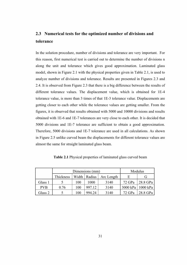
31
2.3 Numerical tests for the optimized number of divisions and
tolerance
In the solution procedure, number of divisions and tolerance are very important. For
this reason, first numerical test is carried out to determine the number of divisions n
along the unit and tolerance which gives good approximation. Laminated glass
model, shown in Figure 2.1 with the physical properties given in Table 2.1, is used to
analyze number of divisions and tolerance. Results are presented in Figures 2.3 and
2.4. It is observed from Figure 2.3 that there is a big difference between the results of
different tolerance values. The displacement value, which is obtained for 1E-4
tolerance value, is more than 3 times of that 1E-3 tolerance value. Displacements are
getting closer to each other while the tolerance values are getting smaller. From the
figures, it is observed that results obtained with 5000 and 10000 divisions and results
obtained with 1E-6 and 1E-7 tolerances are very close to each other. It is decided that
5000 divisions and 1E-7 tolerance are sufficient to obtain a good approximation.
Therefore, 5000 divisions and 1E-7 tolerance are used in all calculations. As shown
in Figure 2.5 unlike curved beam the displacements for different tolerance values are
almost the same for straight laminated glass beam.
Table 2.1 Physical properties of laminated glass curved beam
Dimensions (mm) Modulus Thickness Width Radius Arc Length E G
Glass 1 5 100 1000 3140 72 GPa 28.8 GPa PVB 0.76 100 997.12 3140 3000 kPa 1000 kPa
Glass 2 5 100 994.24 3140 72 GPa 28.8 GPa
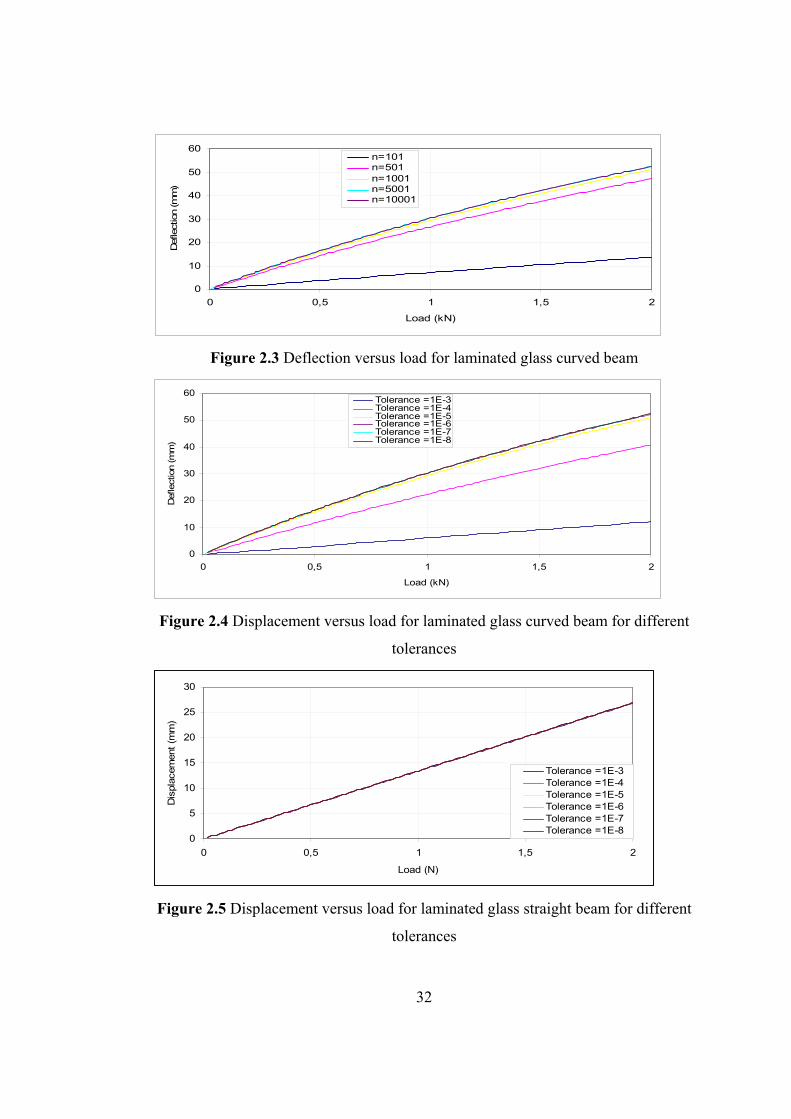
32
0
10
20
30
40
50
60
0 0,5 1 1,5 2
Load (kN)
Def
lect
ion
(mm
)
n=101n=501n=1001n=5001n=10001
Figure 2.3 Deflection versus load for laminated glass curved beam
0
10
20
30
40
50
60
0 0,5 1 1,5 2
Load (kN)
Def
lect
ion
(mm
)
Tolerance =1E-3Tolerance =1E-4Tolerance =1E-5Tolerance =1E-6Tolerance =1E-7Tolerance =1E-8
Figure 2.4 Displacement versus load for laminated glass curved beam for different
tolerances
0
5
10
15
20
25
30
0 0,5 1 1,5 2
Load (N)
Dis
plac
emen
t (m
m)
Tolerance =1E-3Tolerance =1E-4Tolerance =1E-5Tolerance =1E-6Tolerance =1E-7Tolerance =1E-8
Figure 2.5 Displacement versus load for laminated glass straight beam for different
tolerances
33
2.4 Experimental technique and verification of the model for the
curved beam
2.4.1 Finite Element Investigation
In order to verify the developed mathematical model, results are compared with those
of the finite element model for fixed end conditions. The two-dimensional model
developed for the finite element method is developed and solved with ABAQUS
version 6.7-1. Load is concentrated at midspan. Eight node plane stress element
(CPS8R) is used in meshing since it gives more accurate results where large
deformations are involved and leads to faster convergence. The dimensions of the
laminated glass model are 1m outer glass radius, 100 mm width and 5+0.76+5 mm
thickness. The physical properties of laminated glass curved beam are given in Table
2.1. To achieve perfect bound between the layers the surfaces constrained to each
other by using tie option. The Young’s modulus and Poisson’s ratio of glass are
taken to be 72 GPa and 0.25, respectively; but the shear modulus and Poisson’s ratio
of the interlayer are taken as 1000 kPa and 0.29, respectively. To achieve the fixed
end boundary condition for the model, vertical and horizontal degrees of freedom of
all the nodes at both ends of the beams are set to zero. Large deformation analysis is
performed by using nonlinear geometry.
A comparison of the deflections and stresses for laminated fixed supported beam are
presented in Table 2.2 and Figures 2.6 and 2.7. It is observed from Figure 2.6 that
there is almost no difference between the central deflections of the present and finite
element model; maximum error (difference) is about 4.68 %. Comparison of stresses
is presented in Figure 2.7. It is observed Figure 2.7 that the stresses in the finite
element model are higher than those in the model; however, this difference is 3.77%
at most. Therefore, the model developed to analyze the laminated glass beams gives
reliable results for the fixed supported laminated glass curved beams showing
nonlinear behavior.
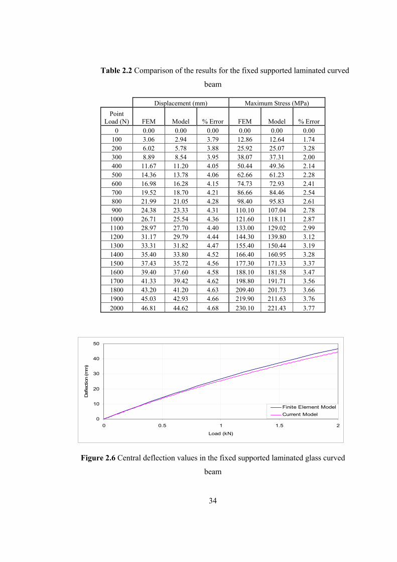
34
Table 2.2 Comparison of the results for the fixed supported laminated curved
beam
Displacement (mm) Maximum Stress (MPa)
Point Load (N) FEM Model % Error FEM Model % Error
0 0.00 0.00 0.00 0.00 0.00 0.00 100 3.06 2.94 3.79 12.86 12.64 1.74 200 6.02 5.78 3.88 25.92 25.07 3.28 300 8.89 8.54 3.95 38.07 37.31 2.00 400 11.67 11.20 4.05 50.44 49.36 2.14 500 14.36 13.78 4.06 62.66 61.23 2.28 600 16.98 16.28 4.15 74.73 72.93 2.41 700 19.52 18.70 4.21 86.66 84.46 2.54 800 21.99 21.05 4.28 98.40 95.83 2.61 900 24.38 23.33 4.31 110.10 107.04 2.78
1000 26.71 25.54 4.36 121.60 118.11 2.87 1100 28.97 27.70 4.40 133.00 129.02 2.99 1200 31.17 29.79 4.44 144.30 139.80 3.12 1300 33.31 31.82 4.47 155.40 150.44 3.19 1400 35.40 33.80 4.52 166.40 160.95 3.28 1500 37.43 35.72 4.56 177.30 171.33 3.37 1600 39.40 37.60 4.58 188.10 181.58 3.47 1700 41.33 39.42 4.62 198.80 191.71 3.56 1800 43.20 41.20 4.63 209.40 201.73 3.66 1900 45.03 42.93 4.66 219.90 211.63 3.76
2000 46.81 44.62 4.68 230.10 221.43 3.77
0
10
20
30
40
50
0 0.5 1 1.5 2
Load (kN)
Def
lect
ion
(mm
)
Finite Element Model
Current Model
Figure 2.6 Central deflection values in the fixed supported laminated glass curved
beam
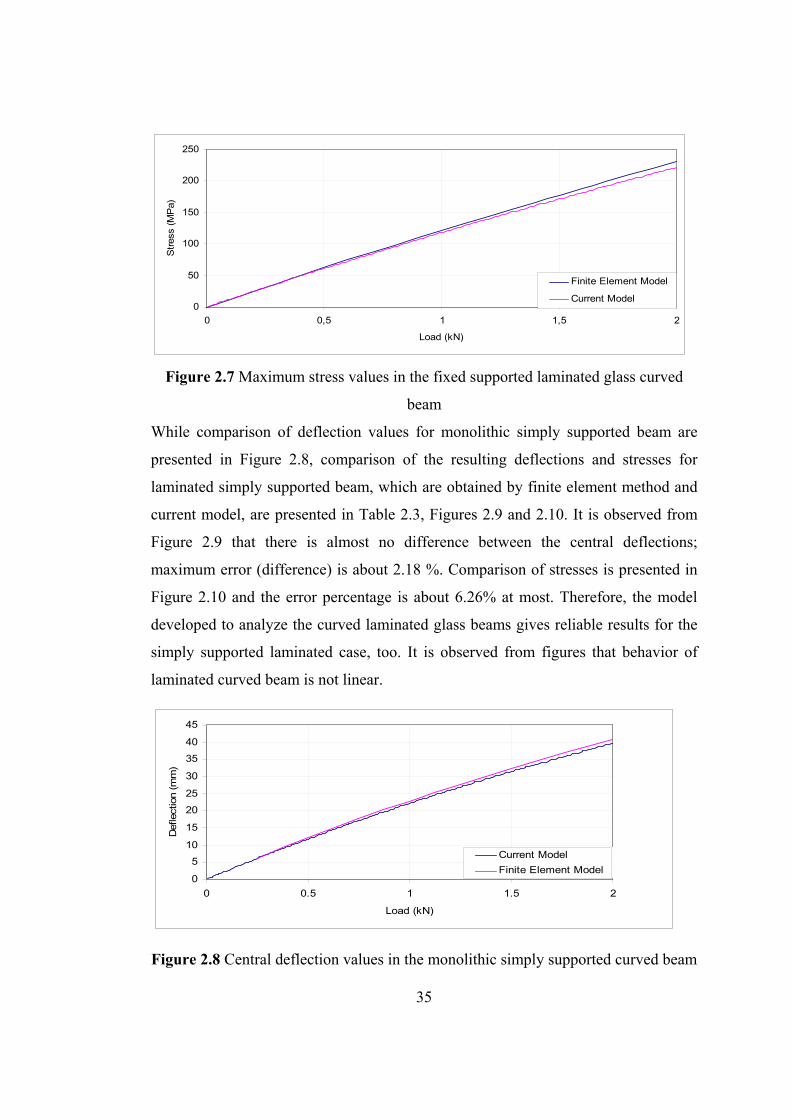
35
0
50
100
150
200
250
0 0,5 1 1,5 2
Load (kN)
Str
ess
(MP
a)
Finite Element Model
Current Model
Figure 2.7 Maximum stress values in the fixed supported laminated glass curved
beam
While comparison of deflection values for monolithic simply supported beam are
presented in Figure 2.8, comparison of the resulting deflections and stresses for
laminated simply supported beam, which are obtained by finite element method and
current model, are presented in Table 2.3, Figures 2.9 and 2.10. It is observed from
Figure 2.9 that there is almost no difference between the central deflections;
maximum error (difference) is about 2.18 %. Comparison of stresses is presented in
Figure 2.10 and the error percentage is about 6.26% at most. Therefore, the model
developed to analyze the curved laminated glass beams gives reliable results for the
simply supported laminated case, too. It is observed from figures that behavior of
laminated curved beam is not linear.
0
5
10
15
20
25
30
35
40
45
0 0.5 1 1.5 2
Load (kN)
Def
lect
ion
(mm
)
Current Model
Finite Element Model
Figure 2.8 Central deflection values in the monolithic simply supported curved beam
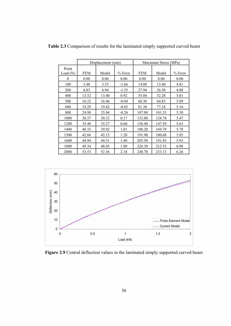
36
Table 2.3 Comparison of results for the laminated simply supported curved beam
Displacement (mm) Maximum Stress (MPa)
Point Load (N) FEM Model % Error FEM Model % Error
0 0.00 0.00 0.00 0.00 0.00 0.00
100 3.48 3.53 -1.66 14.08 13.40 4.81
200 6.83 6.94 -1.55 27.94 26.58 4.88
400 13.52 13.40 0.92 55.04 52.28 5.01
500 16.32 16.46 -0.84 68.30 64.83 5.09
600 19.29 19.42 -0.65 81.38 77.18 5.16
800 24.98 25.04 -0.26 107.00 101.33 5.30
1000 30.37 30.32 0.17 132.00 124.78 5.47
1200 35.48 35.27 0.60 156.40 147.59 5.63
1400 40.33 39.92 1.01 180.20 169.79 5.78
1500 42.66 42.15 1.20 191.90 180.68 5.85
1600 44.94 44.31 1.40 203.50 191.43 5.93
1800 49.34 48.45 1.80 226.30 212.53 6.08
2000 53.53 52.36 2.18 248.70 233.13 6.26
0
10
20
30
40
50
60
0 0.5 1 1.5 2
Load (kN)
Def
lect
ion
(mm
)
Finite Element Model
Current Model
Figure 2.9 Central deflection values in the laminated simply supported curved beam
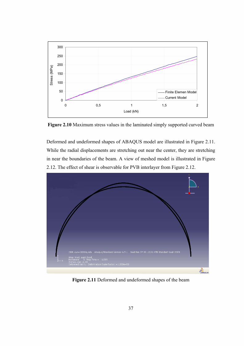
37
0
50
100
150
200
250
300
0 0,5 1 1,5 2
Load (kN)
Str
ess
(MP
a)
Finite Elemen Model
Current Model
Figure 2.10 Maximum stress values in the laminated simply supported curved beam
Deformed and undeformed shapes of ABAQUS model are illustrated in Figure 2.11.
While the radial displacements are stretching out near the center, they are stretching
in near the boundaries of the beam. A view of meshed model is illustrated in Figure
2.12. The effect of shear is observable for PVB interlayer from Figure 2.12.
Figure 2.11 Deformed and undeformed shapes of the beam
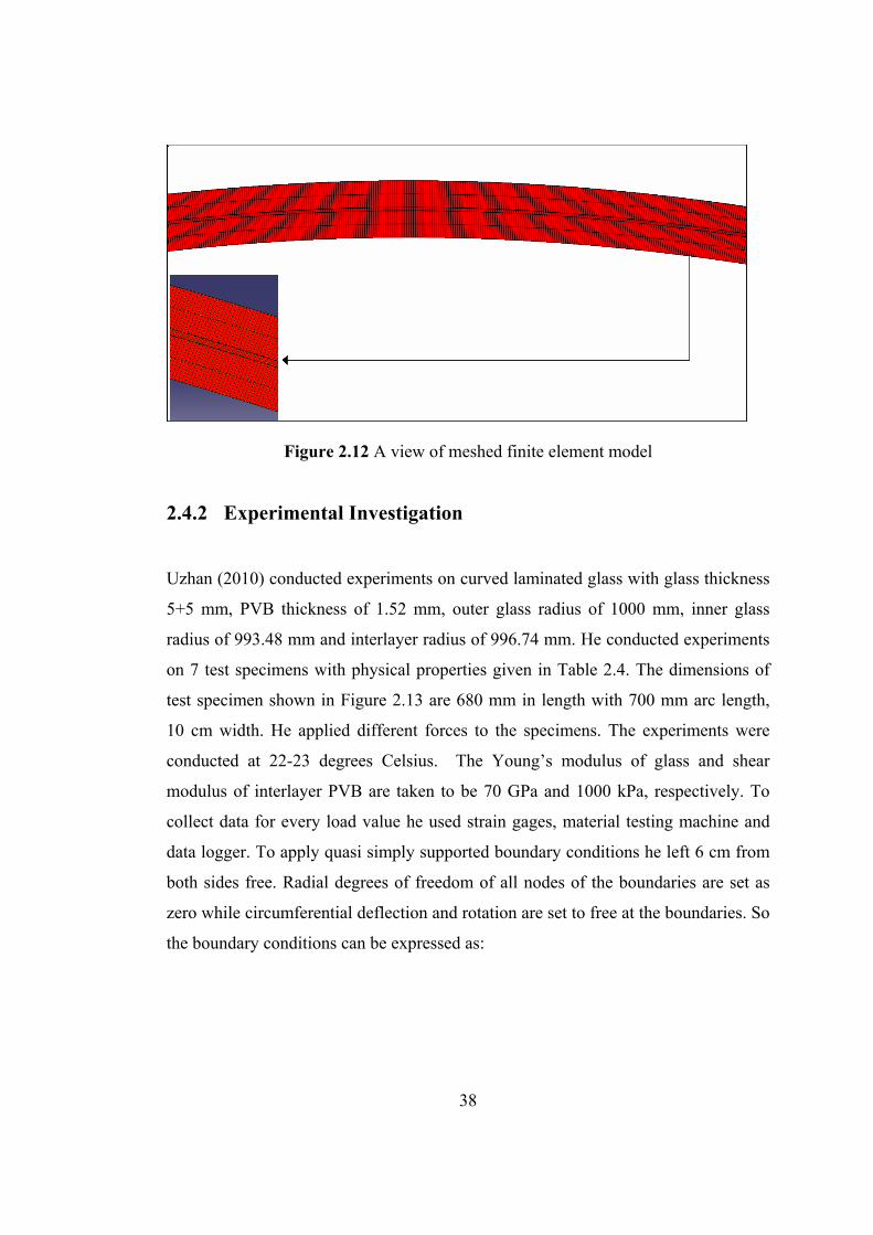
38
Figure 2.12 A view of meshed finite element model
2.4.2 Experimental Investigation Uzhan (2010) conducted experiments on curved laminated glass with glass thickness
5+5 mm, PVB thickness of 1.52 mm, outer glass radius of 1000 mm, inner glass
radius of 993.48 mm and interlayer radius of 996.74 mm. He conducted experiments
on 7 test specimens with physical properties given in Table 2.4. The dimensions of
test specimen shown in Figure 2.13 are 680 mm in length with 700 mm arc length,
10 cm width. He applied different forces to the specimens. The experiments were
conducted at 22-23 degrees Celsius. The Young’s modulus of glass and shear
modulus of interlayer PVB are taken to be 70 GPa and 1000 kPa, respectively. To
collect data for every load value he used strain gages, material testing machine and
data logger. To apply quasi simply supported boundary conditions he left 6 cm from
both sides free. Radial degrees of freedom of all nodes of the boundaries are set as
zero while circumferential deflection and rotation are set to free at the boundaries. So
the boundary conditions can be expressed as:
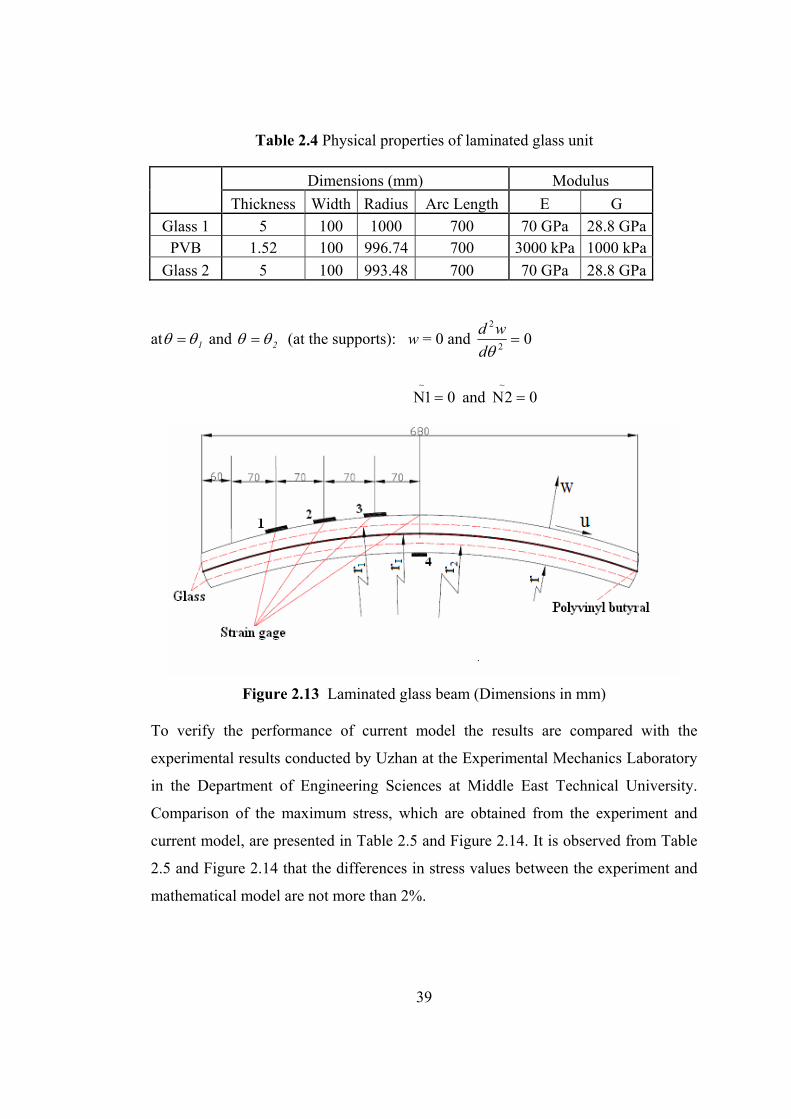
39
Table 2.4 Physical properties of laminated glass unit
Dimensions (mm) Modulus Thickness Width Radius Arc Length E G
Glass 1 5 100 1000 700 70 GPa 28.8 GPa PVB 1.52 100 996.74 700 3000 kPa 1000 kPa
Glass 2 5 100 993.48 700 70 GPa 28.8 GPa
at 1 and 2 (at the supports): w = 0 and 02
2
d
wd
01N~
and 02N~
Figure 2.13 Laminated glass beam (Dimensions in mm)
To verify the performance of current model the results are compared with the
experimental results conducted by Uzhan at the Experimental Mechanics Laboratory
in the Department of Engineering Sciences at Middle East Technical University.
Comparison of the maximum stress, which are obtained from the experiment and
current model, are presented in Table 2.5 and Figure 2.14. It is observed from Table
2.5 and Figure 2.14 that the differences in stress values between the experiment and
mathematical model are not more than 2%.
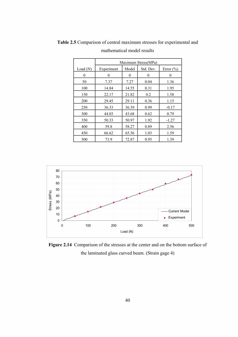
40
Table 2.5 Comparison of central maximum stresses for experimental and
mathematical model results
Maximum Stress(MPa)
Load (N) Experiment Model Std. Dev. Error (%)
0 0 0 0 0
50 7.37 7.27 0.04 1.36
100 14.84 14.55 0.31 1.95
150 22.17 21.82 0.2 1.58
200 29.45 29.11 0.36 1.15
250 36.33 36.39 0.99 -0.17
300 44.03 43.68 0.62 0.79
350 50.33 50.97 1.92 -1.27
400 59.8 58.27 0.89 2.56
450 66.62 65.56 1.03 1.59
500 73.9 72.87 0.95 1.39
0
10
20
30
40
50
60
70
80
0 100 200 300 400 500
Load (N)
Str
ess
(MP
a)
Current Model
Experiment
Figure 2.14 Comparison of the stresses at the center and on the bottom surface of
the laminated glass curved beam. (Strain gage 4)
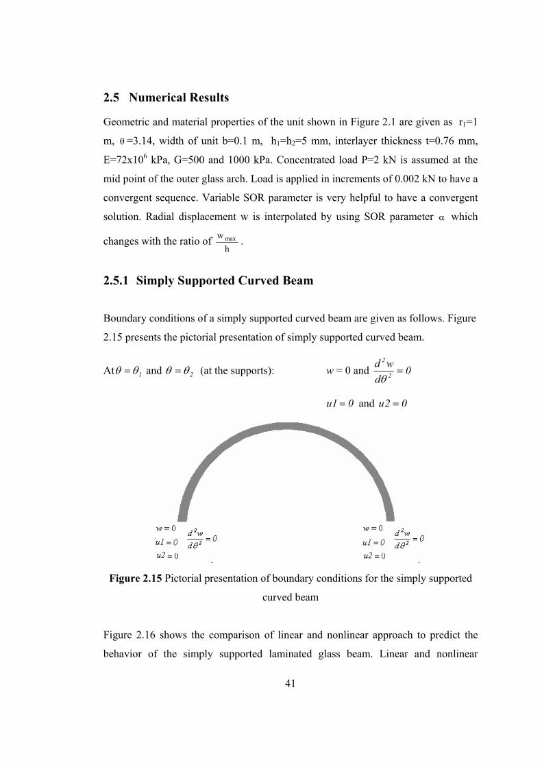
41
2.5 Numerical Results
Geometric and material properties of the unit shown in Figure 2.1 are given as r1=1
m, =3.14, width of unit b=0.1 m, h1=h2=5 mm, interlayer thickness t=0.76 mm,
E=72x106 kPa, G=500 and 1000 kPa. Concentrated load P=2 kN is assumed at the
mid point of the outer glass arch. Load is applied in increments of 0.002 kN to have a
convergent sequence. Variable SOR parameter is very helpful to have a convergent
solution. Radial displacement w is interpolated by using SOR parameter which
changes with the ratio of h
w max .
2.5.1 Simply Supported Curved Beam
Boundary conditions of a simply supported curved beam are given as follows. Figure
2.15 presents the pictorial presentation of simply supported curved beam.
At 1 and 2 (at the supports): w = 0 and 0d
wd2
2
01u and 02u
Figure 2.15 Pictorial presentation of boundary conditions for the simply supported
curved beam
Figure 2.16 shows the comparison of linear and nonlinear approach to predict the
behavior of the simply supported laminated glass beam. Linear and nonlinear
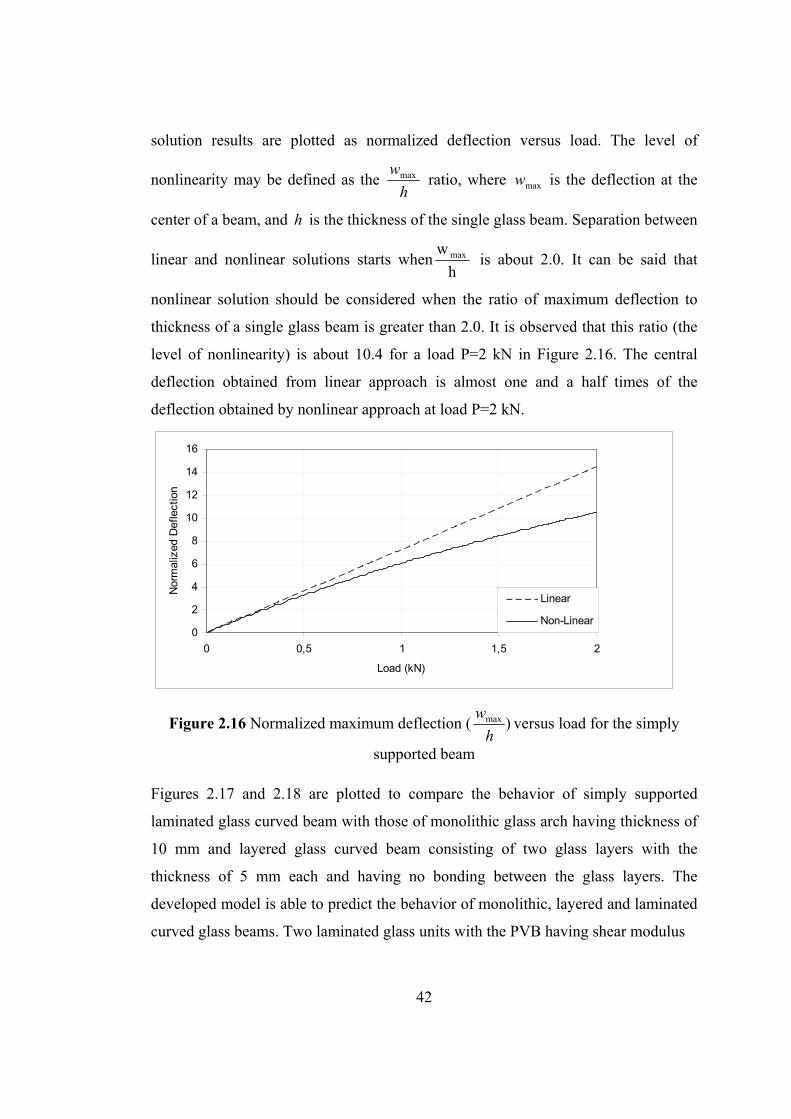
42
solution results are plotted as normalized deflection versus load. The level of
nonlinearity may be defined as the h
wmax ratio, where maxw is the deflection at the
center of a beam, and h is the thickness of the single glass beam. Separation between
linear and nonlinear solutions starts whenh
w max is about 2.0. It can be said that
nonlinear solution should be considered when the ratio of maximum deflection to
thickness of a single glass beam is greater than 2.0. It is observed that this ratio (the
level of nonlinearity) is about 10.4 for a load P=2 kN in Figure 2.16. The central
deflection obtained from linear approach is almost one and a half times of the
deflection obtained by nonlinear approach at load P=2 kN.
0
2
4
6
8
10
12
14
16
0 0,5 1 1,5 2
Load (kN)
Nor
mal
ized
Def
lect
ion
Linear
Non-Linear
Figure 2.16 Normalized maximum deflection ( )max
h
wversus load for the simply
supported beam Figures 2.17 and 2.18 are plotted to compare the behavior of simply supported
laminated glass curved beam with those of monolithic glass arch having thickness of
10 mm and layered glass curved beam consisting of two glass layers with the
thickness of 5 mm each and having no bonding between the glass layers. The
developed model is able to predict the behavior of monolithic, layered and laminated
curved glass beams. Two laminated glass units with the PVB having shear modulus
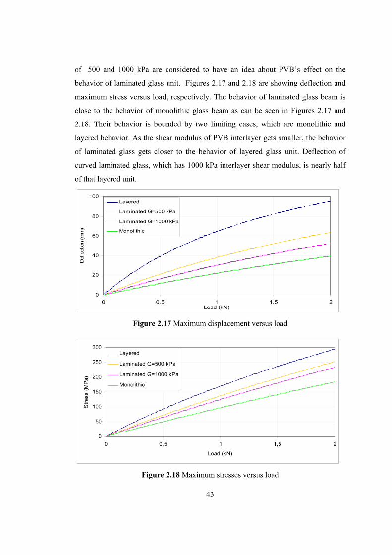
43
of 500 and 1000 kPa are considered to have an idea about PVB’s effect on the
behavior of laminated glass unit. Figures 2.17 and 2.18 are showing deflection and
maximum stress versus load, respectively. The behavior of laminated glass beam is
close to the behavior of monolithic glass beam as can be seen in Figures 2.17 and
2.18. Their behavior is bounded by two limiting cases, which are monolithic and
layered behavior. As the shear modulus of PVB interlayer gets smaller, the behavior
of laminated glass gets closer to the behavior of layered glass unit. Deflection of
curved laminated glass, which has 1000 kPa interlayer shear modulus, is nearly half
of that layered unit.
0
20
40
60
80
100
0 0.5 1 1.5 2Load (kN)
Def
lect
ion
(mm
)
Layered
Laminated G=500 kPa
Laminated G=1000 kPa
Monolithic
Figure 2.17 Maximum displacement versus load
0
50
100
150
200
250
300
0 0,5 1 1,5 2
Load (kN)
Str
ess
(MP
a)
Layered
Laminated G=500 kPa
Laminated G=1000 kPa
Monolithic
Figure 2.18 Maximum stresses versus load
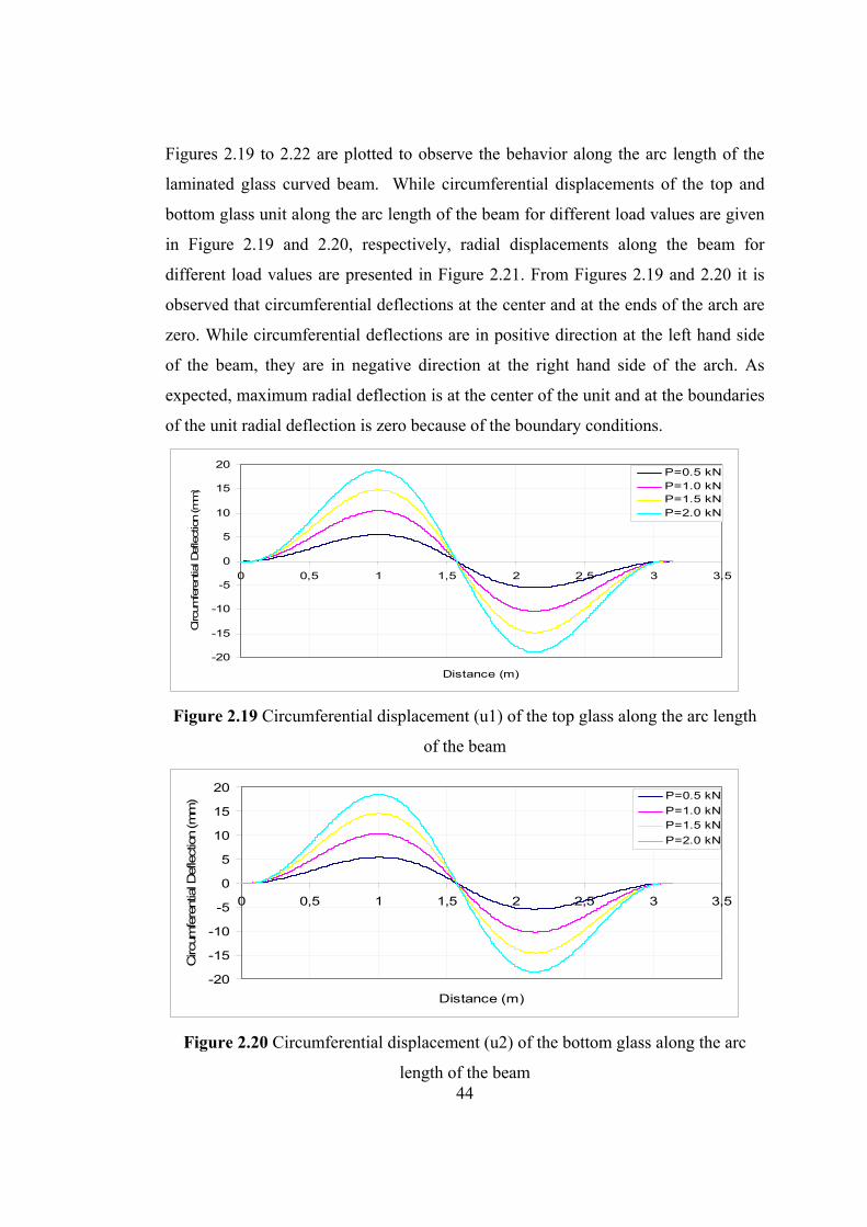
44
Figures 2.19 to 2.22 are plotted to observe the behavior along the arc length of the
laminated glass curved beam. While circumferential displacements of the top and
bottom glass unit along the arc length of the beam for different load values are given
in Figure 2.19 and 2.20, respectively, radial displacements along the beam for
different load values are presented in Figure 2.21. From Figures 2.19 and 2.20 it is
observed that circumferential deflections at the center and at the ends of the arch are
zero. While circumferential deflections are in positive direction at the left hand side
of the beam, they are in negative direction at the right hand side of the arch. As
expected, maximum radial deflection is at the center of the unit and at the boundaries
of the unit radial deflection is zero because of the boundary conditions.
-20
-15
-10
-5
0
5
10
15
20
0 0,5 1 1,5 2 2,5 3 3,5
Distance (m)
Circ
umfe
rent
ial D
efle
ctio
n (m
m)
P=0.5 kNP=1.0 kNP=1.5 kNP=2.0 kN
Figure 2.19 Circumferential displacement (u1) of the top glass along the arc length
of the beam
-20
-15
-10
-5
0
5
10
15
20
0 0,5 1 1,5 2 2,5 3 3,5
Distance (m)
Circ
umfe
rent
ial D
efle
ctio
n (m
m) P=0.5 kN
P=1.0 kNP=1.5 kN
P=2.0 kN
Figure 2.20 Circumferential displacement (u2) of the bottom glass along the arc
length of the beam
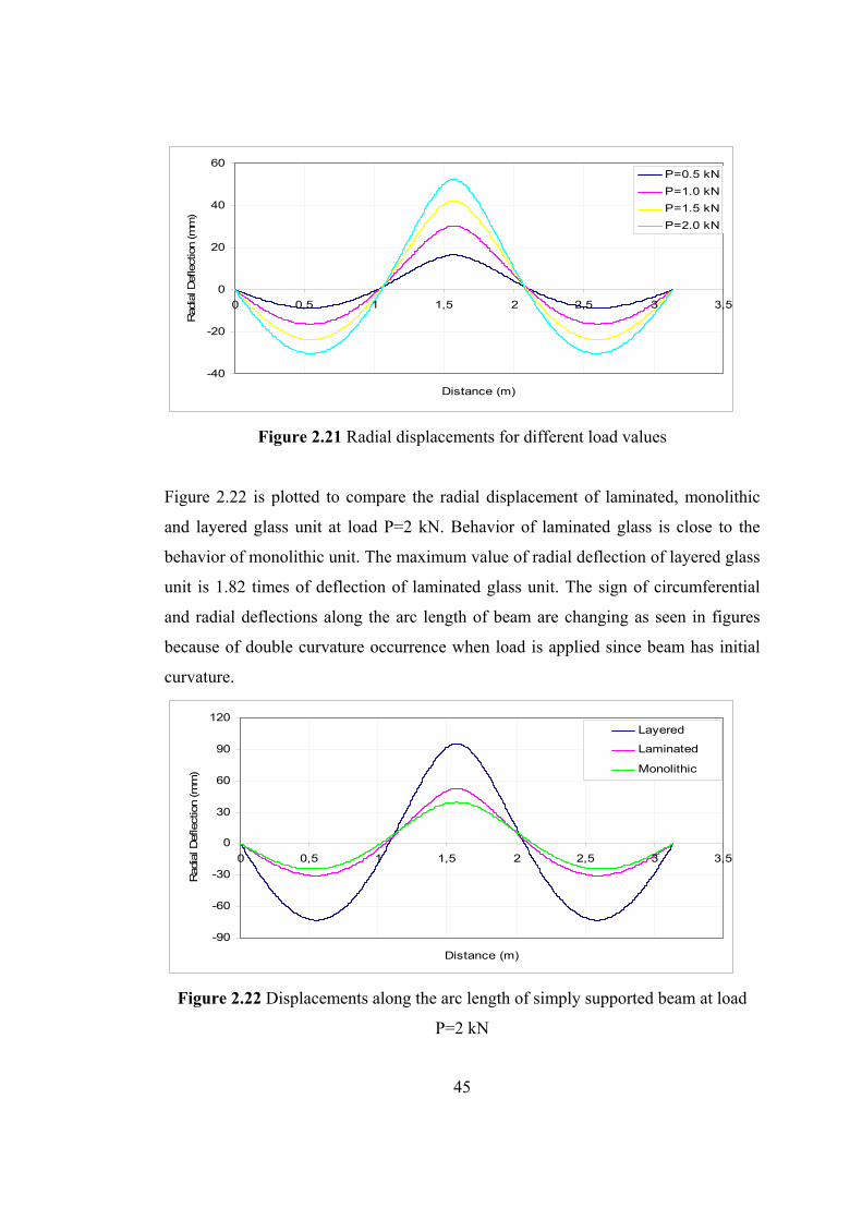
45
-40
-20
0
20
40
60
0 0,5 1 1,5 2 2,5 3 3,5
Distance (m)
Rad
ial D
efle
ctio
n (m
m)
P=0.5 kN
P=1.0 kN
P=1.5 kN
P=2.0 kN
Figure 2.21 Radial displacements for different load values
Figure 2.22 is plotted to compare the radial displacement of laminated, monolithic
and layered glass unit at load P=2 kN. Behavior of laminated glass is close to the
behavior of monolithic unit. The maximum value of radial deflection of layered glass
unit is 1.82 times of deflection of laminated glass unit. The sign of circumferential
and radial deflections along the arc length of beam are changing as seen in figures
because of double curvature occurrence when load is applied since beam has initial
curvature.
-90
-60
-30
0
30
60
90
120
0 0,5 1 1,5 2 2,5 3 3,5
Distance (m)
Rad
ial D
efle
ctio
n (m
m)
Layered
Laminated
Monolithic
Figure 2.22 Displacements along the arc length of simply supported beam at load
P=2 kN
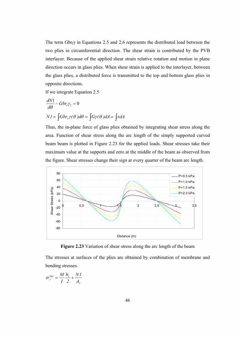
46
The term GbrIγ in Equations 2.5 and 2.6 represents the distributed load between the
two plies in circumferential direction. The shear strain is contributed by the PVB
interlayer. Because of the applied shear strain relative rotation and motion in plane
direction occurs in glass plies. When shear strain is applied to the interlayer, between
the glass plies, a distributed force is transmitted to the top and bottom glass plies in
opposite directions.
If we integrate Equation 2.5
01
IIGbrd
dN
dAdA)(Gd)(Gbr1N I
Thus, the in-plane force of glass plies obtained by integrating shear stress along the
area. Function of shear stress along the arc length of the simply supported curved
beam beam is plotted in Figure 2.23 for the applied loads. Shear stresses take their
maximum value at the supports and zero at the middle of the beam as observed from
the figure. Shear stresses change their sign at every quarter of the beam arc length.
-80
-60
-40
-20
0
20
40
60
80
0 0,5 1 1,5 2 2,5 3 3,5
Distance (m)
She
ar S
tres
s (k
Pa)
P=0.5 kPa
P=1.0 kPa
P=1.5 kPa
P=2.0 kPa
Figure 2.23 Variation of shear stress along the arc length of the beam
The stresses at surfaces of the plies are obtained by combination of membrane and
bending stresses.
1
1top1 A
1N
2
h
I
M
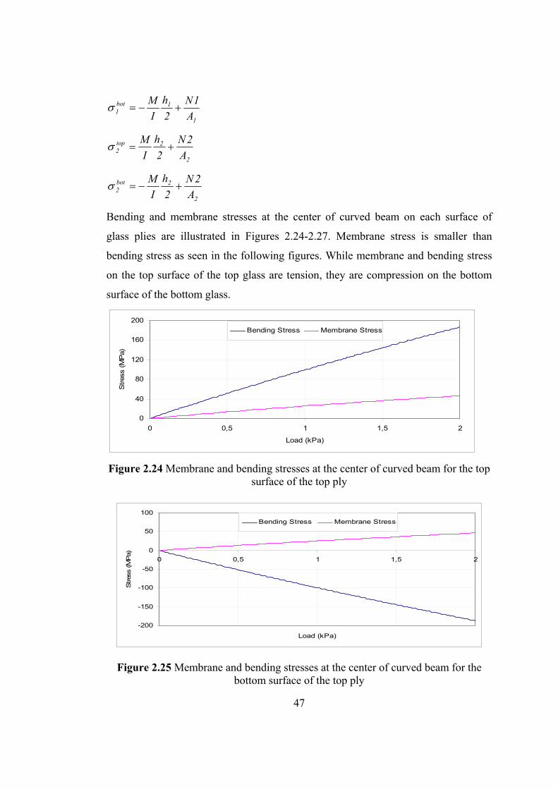
47
1
1bot1 A
1N
2
h
I
M
2
2top2 A
2N
2
h
I
M
2
2bot2 A
2N
2
h
I
M
Bending and membrane stresses at the center of curved beam on each surface of
glass plies are illustrated in Figures 2.24-2.27. Membrane stress is smaller than
bending stress as seen in the following figures. While membrane and bending stress
on the top surface of the top glass are tension, they are compression on the bottom
surface of the bottom glass.
0
40
80
120
160
200
0 0,5 1 1,5 2
Load (kPa)
Stres
s (M
Pa)
Bending Stress Membrane Stress
Figure 2.24 Membrane and bending stresses at the center of curved beam for the top surface of the top ply
-200
-150
-100
-50
0
50
100
0 0,5 1 1,5 2
Load (kPa)
Stres
s (M
Pa)
Bending Stress Membrane Stress
Figure 2.25 Membrane and bending stresses at the center of curved beam for the bottom surface of the top ply
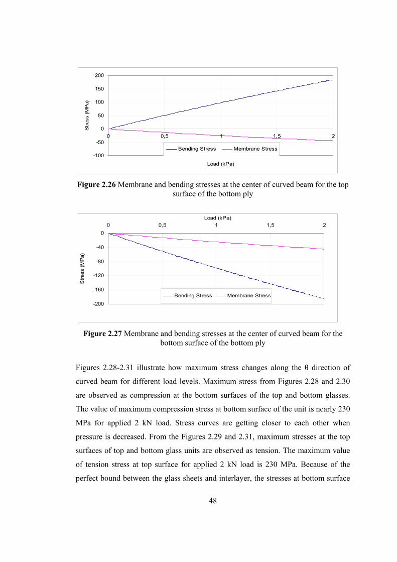
48
-100
-50
0
50
100
150
200
0 0,5 1 1,5 2
Load (kPa)
Str
ess
(MP
a)
Bending Stress Membrane Stress
Figure 2.26 Membrane and bending stresses at the center of curved beam for the top surface of the bottom ply
-200
-160
-120
-80
-40
0
0 0,5 1 1,5 2Load (kPa)
Str
ess
(MP
a)
Bending Stress Membrane Stress
Figure 2.27 Membrane and bending stresses at the center of curved beam for the bottom surface of the bottom ply
Figures 2.28-2.31 illustrate how maximum stress changes along the θ direction of
curved beam for different load levels. Maximum stress from Figures 2.28 and 2.30
are observed as compression at the bottom surfaces of the top and bottom glasses.
The value of maximum compression stress at bottom surface of the unit is nearly 230
MPa for applied 2 kN load. Stress curves are getting closer to each other when
pressure is decreased. From the Figures 2.29 and 2.31, maximum stresses at the top
surfaces of top and bottom glass units are observed as tension. The maximum value
of tension stress at top surface for applied 2 kN load is 230 MPa. Because of the
perfect bound between the glass sheets and interlayer, the stresses at bottom surface
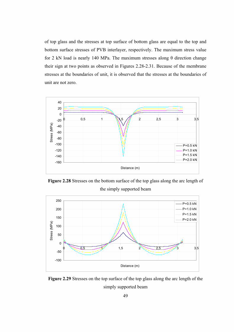
49
of top glass and the stresses at top surface of bottom glass are equal to the top and
bottom surface stresses of PVB interlayer, respectively. The maximum stress value
for 2 kN load is nearly 140 MPa. The maximum stresses along θ direction change
their sign at two points as observed in Figures 2.28-2.31. Because of the membrane
stresses at the boundaries of unit, it is observed that the stresses at the boundaries of
unit are not zero.
-160
-140
-120
-100
-80
-60
-40
-20
0
20
40
0 0,5 1 1,5 2 2,5 3 3,5
Distance (m)
Str
ess
(MP
a)
P=0.5 kN
P=1.0 kNP=1.5 kN
P=2.0 kN
Figure 2.28 Stresses on the bottom surface of the top glass along the arc length of
the simply supported beam
-100
-50
0
50
100
150
200
250
0 0,5 1 1,5 2 2,5 3 3,5
Distance (m)
Str
ess
(MP
a)
P=0.5 kN
P=1.0 kN
P=1.5 kN
P=2.0 kN
Figure 2.29 Stresses on the top surface of the top glass along the arc length of the
simply supported beam
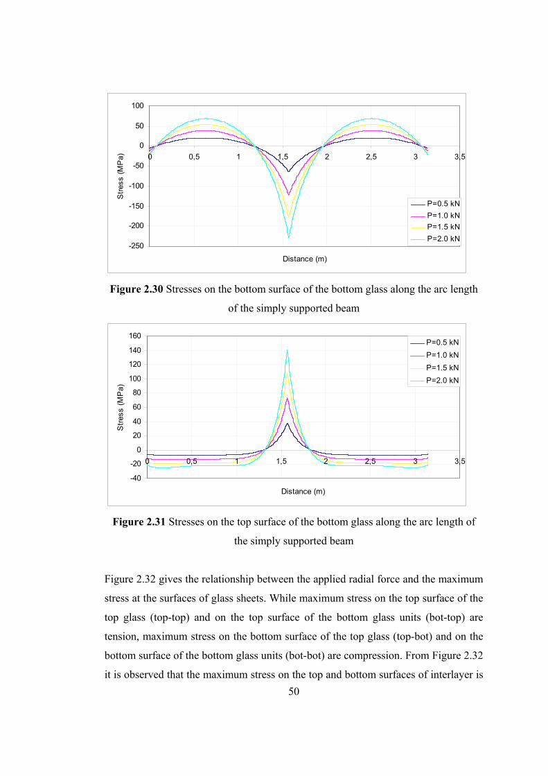
50
-250
-200
-150
-100
-50
0
50
100
0 0,5 1 1,5 2 2,5 3 3,5
Distance (m)
Str
ess
(MP
a)
P=0.5 kN
P=1.0 kN
P=1.5 kN
P=2.0 kN
Figure 2.30 Stresses on the bottom surface of the bottom glass along the arc length
of the simply supported beam
-40
-20
0
20
40
60
80
100
120
140
160
0 0,5 1 1,5 2 2,5 3 3,5
Distance (m)
Str
ess
(MP
a)
P=0.5 kN
P=1.0 kN
P=1.5 kN
P=2.0 kN
Figure 2.31 Stresses on the top surface of the bottom glass along the arc length of
the simply supported beam
Figure 2.32 gives the relationship between the applied radial force and the maximum
stress at the surfaces of glass sheets. While maximum stress on the top surface of the
top glass (top-top) and on the top surface of the bottom glass units (bot-top) are
tension, maximum stress on the bottom surface of the top glass (top-bot) and on the
bottom surface of the bottom glass units (bot-bot) are compression. From Figure 2.32
it is observed that the maximum stress on the top and bottom surfaces of interlayer is
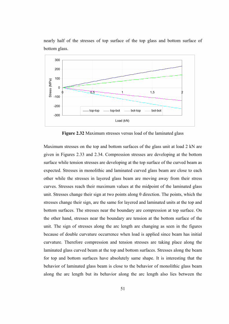
51
nearly half of the stresses of top surface of the top glass and bottom surface of
bottom glass.
-300
-200
-100
0
100
200
300
0 0,5 1 1,5 2
Load (kN)
Str
ess
(MP
a)
top-top top-bot bot-top bot-bot
Figure 2.32 Maximum stresses versus load of the laminated glass
Maximum stresses on the top and bottom surfaces of the glass unit at load 2 kN are
given in Figures 2.33 and 2.34. Compression stresses are developing at the bottom
surface while tension stresses are developing at the top surface of the curved beam as
expected. Stresses in monolithic and laminated curved glass beam are close to each
other while the stresses in layered glass beam are moving away from their stress
curves. Stresses reach their maximum values at the midpoint of the laminated glass
unit. Stresses change their sign at two points along θ direction. The points, which the
stresses change their sign, are the same for layered and laminated units at the top and
bottom surfaces. The stresses near the boundary are compression at top surface. On
the other hand, stresses near the boundary are tension at the bottom surface of the
unit. The sign of stresses along the arc length are changing as seen in the figures
because of double curvature occurrence when load is applied since beam has initial
curvature. Therefore compression and tension stresses are taking place along the
laminated glass curved beam at the top and bottom surfaces. Stresses along the beam
for top and bottom surfaces have absolutely same shape. It is interesting that the
behavior of laminated glass beam is close to the behavior of monolithic glass beam
along the arc length but its behavior along the arc length also lies between the
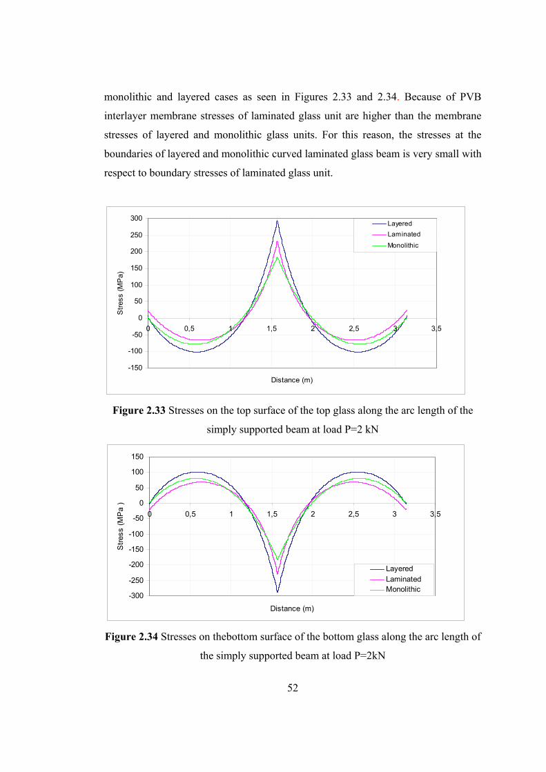
52
monolithic and layered cases as seen in Figures 2.33 and 2.34. Because of PVB
interlayer membrane stresses of laminated glass unit are higher than the membrane
stresses of layered and monolithic glass units. For this reason, the stresses at the
boundaries of layered and monolithic curved laminated glass beam is very small with
respect to boundary stresses of laminated glass unit.
-150
-100
-50
0
50
100
150
200
250
300
0 0,5 1 1,5 2 2,5 3 3,5
Distance (m)
Str
ess
(MP
a)
Layered
Laminated
Monolithic
Figure 2.33 Stresses on the top surface of the top glass along the arc length of the
simply supported beam at load P=2 kN
-300
-250
-200
-150
-100
-50
0
50
100
150
0 0,5 1 1,5 2 2,5 3 3,5
Distance (m)
Str
ess
(MP
a )
LayeredLaminatedMonolithic
Figure 2.34 Stresses on thebottom surface of the bottom glass along the arc length of
the simply supported beam at load P=2kN
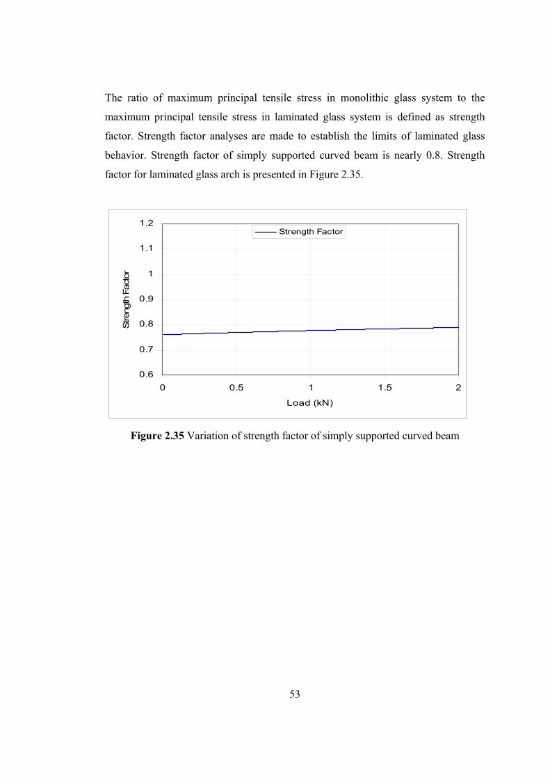
53
The ratio of maximum principal tensile stress in monolithic glass system to the
maximum principal tensile stress in laminated glass system is defined as strength
factor. Strength factor analyses are made to establish the limits of laminated glass
behavior. Strength factor of simply supported curved beam is nearly 0.8. Strength
factor for laminated glass arch is presented in Figure 2.35.
0.6
0.7
0.8
0.9
1
1.1
1.2
0 0.5 1 1.5 2
Load (kN)
Strength
Fact
or
Strength Factor
Figure 2.35 Variation of strength factor of simply supported curved beam
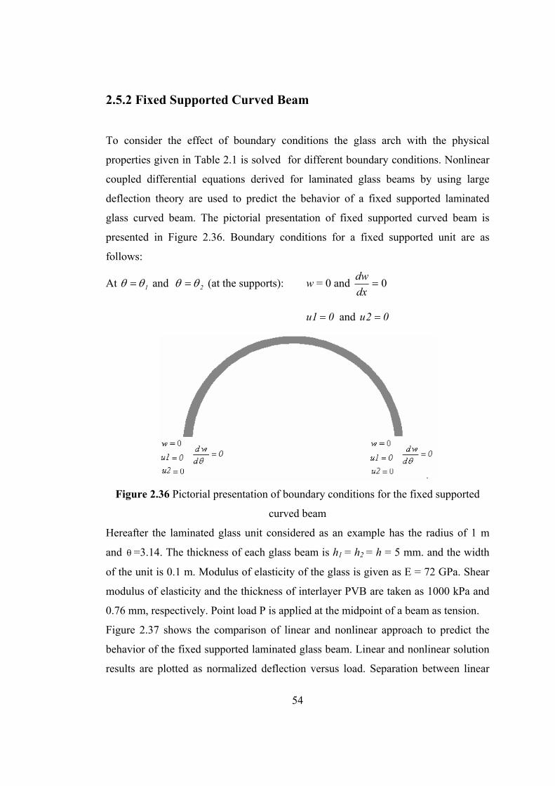
54
2.5.2 Fixed Supported Curved Beam
To consider the effect of boundary conditions the glass arch with the physical
properties given in Table 2.1 is solved for different boundary conditions. Nonlinear
coupled differential equations derived for laminated glass beams by using large
deflection theory are used to predict the behavior of a fixed supported laminated
glass curved beam. The pictorial presentation of fixed supported curved beam is
presented in Figure 2.36. Boundary conditions for a fixed supported unit are as
follows:
At 1 and 2 (at the supports): w = 0 and 0dx
dw
01u and 02u
Figure 2.36 Pictorial presentation of boundary conditions for the fixed supported
curved beam
Hereafter the laminated glass unit considered as an example has the radius of 1 m
and =3.14. The thickness of each glass beam is h1 = h2 = h = 5 mm. and the width
of the unit is 0.1 m. Modulus of elasticity of the glass is given as E = 72 GPa. Shear
modulus of elasticity and the thickness of interlayer PVB are taken as 1000 kPa and
0.76 mm, respectively. Point load P is applied at the midpoint of a beam as tension.
Figure 2.37 shows the comparison of linear and nonlinear approach to predict the
behavior of the fixed supported laminated glass beam. Linear and nonlinear solution
results are plotted as normalized deflection versus load. Separation between linear
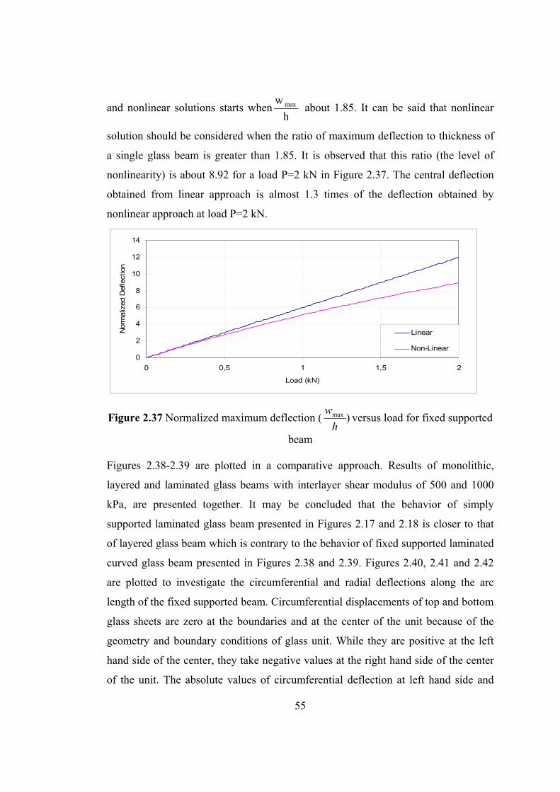
55
and nonlinear solutions starts whenh
w max about 1.85. It can be said that nonlinear
solution should be considered when the ratio of maximum deflection to thickness of
a single glass beam is greater than 1.85. It is observed that this ratio (the level of
nonlinearity) is about 8.92 for a load P=2 kN in Figure 2.37. The central deflection
obtained from linear approach is almost 1.3 times of the deflection obtained by
nonlinear approach at load P=2 kN.
0
2
4
6
8
10
12
14
0 0,5 1 1,5 2
Load (kN)
Nor
mal
ized
Def
lect
ion
Linear
Non-Linear
Figure 2.37 Normalized maximum deflection ( )max
h
wversus load for fixed supported
beam
Figures 2.38-2.39 are plotted in a comparative approach. Results of monolithic,
layered and laminated glass beams with interlayer shear modulus of 500 and 1000
kPa, are presented together. It may be concluded that the behavior of simply
supported laminated glass beam presented in Figures 2.17 and 2.18 is closer to that
of layered glass beam which is contrary to the behavior of fixed supported laminated
curved glass beam presented in Figures 2.38 and 2.39. Figures 2.40, 2.41 and 2.42
are plotted to investigate the circumferential and radial deflections along the arc
length of the fixed supported beam. Circumferential displacements of top and bottom
glass sheets are zero at the boundaries and at the center of the unit because of the
geometry and boundary conditions of glass unit. While they are positive at the left
hand side of the center, they take negative values at the right hand side of the center
of the unit. The absolute values of circumferential deflection at left hand side and
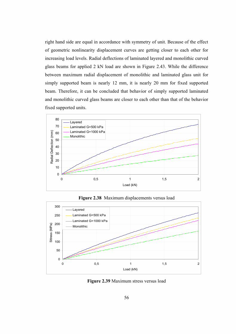
56
right hand side are equal in accordance with symmetry of unit. Because of the effect
of geometric nonlinearity displacement curves are getting closer to each other for
increasing load levels. Radial deflections of laminated layered and monolithic curved
glass beams for applied 2 kN load are shown in Figure 2.43. While the difference
between maximum radial displacement of monolithic and laminated glass unit for
simply supported beam is nearly 12 mm, it is nearly 20 mm for fixed supported
beam. Therefore, it can be concluded that behavior of simply supported laminated
and monolithic curved glass beams are closer to each other than that of the behavior
fixed supported units.
0
10
20
30
40
50
60
70
80
0 0,5 1 1,5 2
Load (kN)
Rad
ial D
efle
ctio
n (m
m)
Layered
Laminated G=500 kPa
Laminated G=1000 kPaMonolithic
Figure 2.38 Maximum displacements versus load
0
50
100
150
200
250
300
0 0,5 1 1,5 2
Load (kN)
Stt
ress
(M
Pa)
Layered
Laminated G=500 kPa
Laminated G=1000 kPa
Monolithic
Figure 2.39 Maximum stress versus load
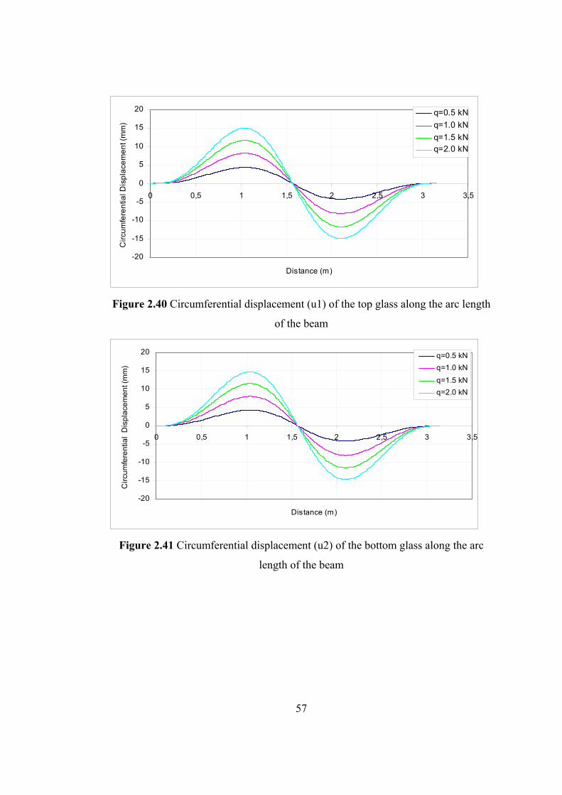
57
-20
-15
-10
-5
0
5
10
15
20
0 0,5 1 1,5 2 2,5 3 3,5
Distance (m)
Cir
cum
fere
ntia
l Dis
pla
cem
en
t (m
m)
q=0.5 kN
q=1.0 kN
q=1.5 kNq=2.0 kN
Figure 2.40 Circumferential displacement (u1) of the top glass along the arc length
of the beam
-20
-15
-10
-5
0
5
10
15
20
0 0,5 1 1,5 2 2,5 3 3,5
Distance (m)
Cir
cum
fere
ntia
l D
isp
lace
me
nt (
mm
)
q=0.5 kN
q=1.0 kN
q=1.5 kN
q=2.0 kN
Figure 2.41 Circumferential displacement (u2) of the bottom glass along the arc
length of the beam
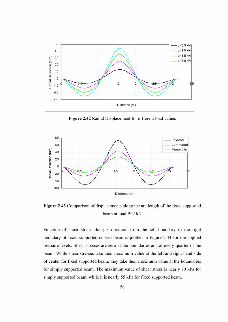
58
-30
-20
-10
0
10
20
30
40
50
0 0,5 1 1,5 2 2,5 3 3,5
Distance (m)
Ra
dia
l De
flect
ion
(m
m)
q=0.5 kN
q=1.0 kN
q=1.5 kN
q=2.0 kN
Figure 2.42 Radial Displacement for different load values
-60
-40
-20
0
20
40
60
80
0 0,5 1 1,5 2 2,5 3 3,5
Distance (m)
Radia
l Defle
ctio
n (m
m)
Layered
Laminated
Monolithic
Figure 2.43 Comparison of displacements along the arc length of the fixed supported
beam at load P=2 kN
Function of shear stress along θ direction from the left boundary to the right
boundary of fixed supported curved beam is plotted in Figure 2.44 for the applied
pressure levels. Shear stresses are zero at the boundaries and at every quarter of the
beam. While shear stresses take their maximum value at the left and right hand side
of center for fixed supported beam, they take their maximum value at the boundaries
for simply supported beam. The maximum value of shear stress is nearly 70 kPa for
simply supported beam, while it is nearly 55 kPa for fixed supported beam.
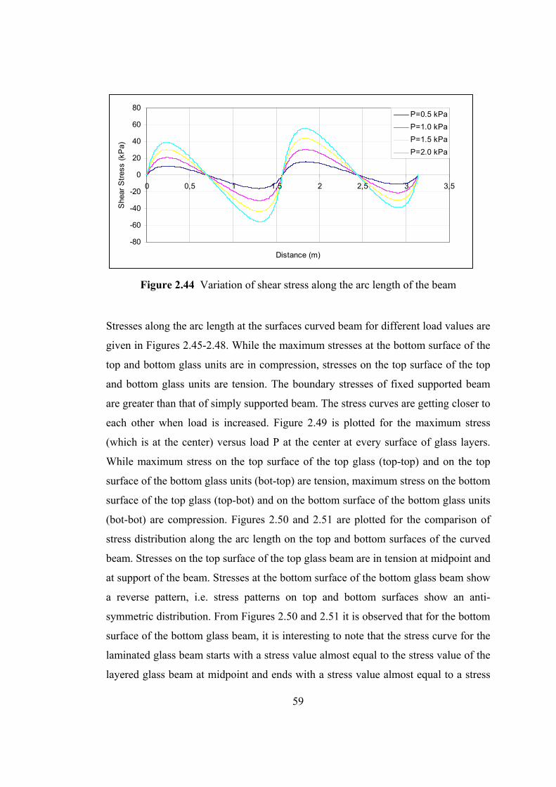
59
-80
-60
-40
-20
0
20
40
60
80
0 0,5 1 1,5 2 2,5 3 3,5
Distance (m)
She
ar S
tres
s (k
Pa)
P=0.5 kPa
P=1.0 kPa
P=1.5 kPa
P=2.0 kPa
Figure 2.44 Variation of shear stress along the arc length of the beam
Stresses along the arc length at the surfaces curved beam for different load values are
given in Figures 2.45-2.48. While the maximum stresses at the bottom surface of the
top and bottom glass units are in compression, stresses on the top surface of the top
and bottom glass units are tension. The boundary stresses of fixed supported beam
are greater than that of simply supported beam. The stress curves are getting closer to
each other when load is increased. Figure 2.49 is plotted for the maximum stress
(which is at the center) versus load P at the center at every surface of glass layers.
While maximum stress on the top surface of the top glass (top-top) and on the top
surface of the bottom glass units (bot-top) are tension, maximum stress on the bottom
surface of the top glass (top-bot) and on the bottom surface of the bottom glass units
(bot-bot) are compression. Figures 2.50 and 2.51 are plotted for the comparison of
stress distribution along the arc length on the top and bottom surfaces of the curved
beam. Stresses on the top surface of the top glass beam are in tension at midpoint and
at support of the beam. Stresses at the bottom surface of the bottom glass beam show
a reverse pattern, i.e. stress patterns on top and bottom surfaces show an anti-
symmetric distribution. From Figures 2.50 and 2.51 it is observed that for the bottom
surface of the bottom glass beam, it is interesting to note that the stress curve for the
laminated glass beam starts with a stress value almost equal to the stress value of the
layered glass beam at midpoint and ends with a stress value almost equal to a stress
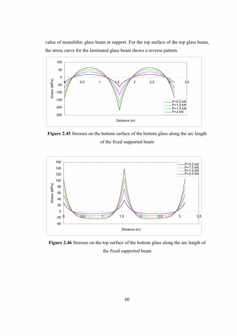
60
value of monolithic glass beam at support. For the top surface of the top glass beam,
the stress curve for the laminated glass beam shows a reverse pattern.
-250
-200
-150
-100
-50
0
50
100
0 0,5 1 1,5 2 2,5 3 3,5
Distance (m)
Str
ess
(MP
a)
P=0.5 kNP=1.0 kNP=1.5 kNP=2 kN
Figure 2.45 Stresses on the bottom surface of the bottom glass along the arc length
of the fixed supported beam
-40
-20
0
20
40
60
80
100
120
140
160
0 0,5 1 1,5 2 2,5 3 3,5
Distance (m)
Str
ess
(MP
a)
P=0.5 kNP=1.0 kNP=1.5 kNP=2.0 kN
Figure 2.46 Stresses on the top surface of the bottom glass along the arc length of
the fixed supported beam
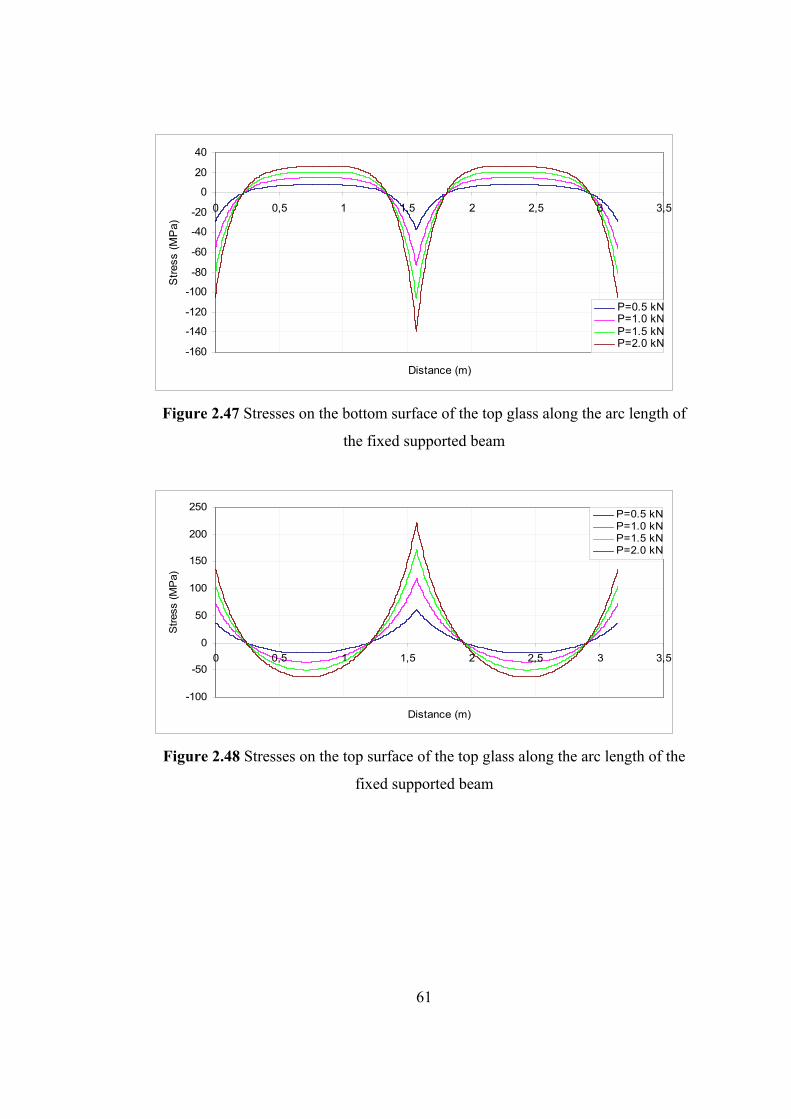
61
-160
-140
-120
-100
-80
-60
-40
-20
0
20
40
0 0,5 1 1,5 2 2,5 3 3,5
Distance (m)
Str
ess
(MP
a)
P=0.5 kNP=1.0 kNP=1.5 kNP=2.0 kN
Figure 2.47 Stresses on the bottom surface of the top glass along the arc length of
the fixed supported beam
-100
-50
0
50
100
150
200
250
0 0,5 1 1,5 2 2,5 3 3,5
Distance (m)
Str
ess
(MP
a)
P=0.5 kNP=1.0 kNP=1.5 kNP=2.0 kN
Figure 2.48 Stresses on the top surface of the top glass along the arc length of the
fixed supported beam
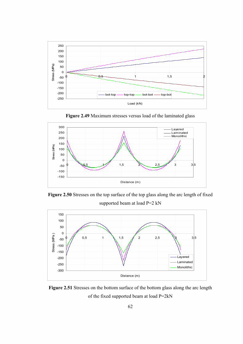
62
-250
-200
-150
-100
-50
0
50
100
150
200
250
0 0,5 1 1,5 2
Load (kN)
Stres
s (M
Pa)
bot-top top-top bot-bot top-bot
Figure 2.49 Maximum stresses versus load of the laminated glass
-150
-100
-50
0
50
100
150
200
250
300
0 0,5 1 1,5 2 2,5 3 3,5
Distance (m)
Stres
s (M
Pa)
LayeredLaminatedMonolithic
Figure 2.50 Stresses on the top surface of the top glass along the arc length of fixed
supported beam at load P=2 kN
-300
-250
-200
-150
-100
-50
0
50
100
150
0 0,5 1 1,5 2 2,5 3 3,5
Distance (m)
Str
ess
(MP
a )
Layered
Laminated
Monolithic
Figure 2.51 Stresses on the bottom surface of the bottom glass along the arc length
of the fixed supported beam at load P=2kN
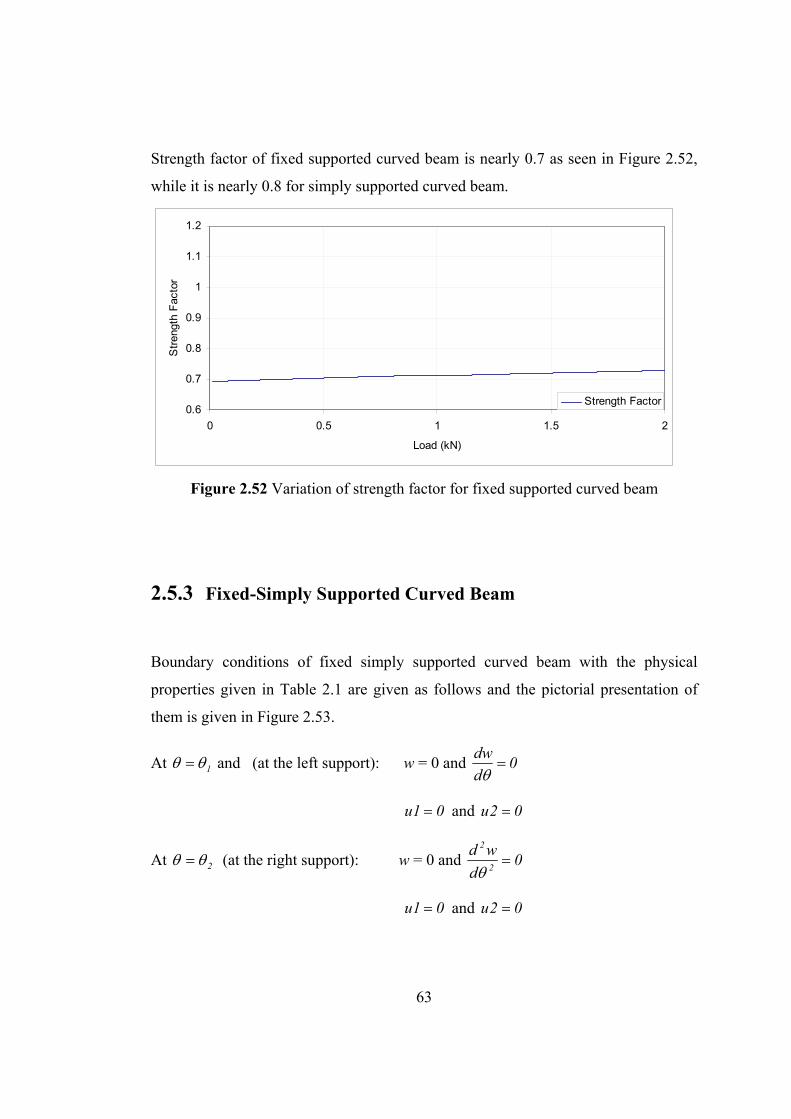
63
Strength factor of fixed supported curved beam is nearly 0.7 as seen in Figure 2.52,
while it is nearly 0.8 for simply supported curved beam.
0.6
0.7
0.8
0.9
1
1.1
1.2
0 0.5 1 1.5 2
Load (kN)
Str
engt
h F
acto
r
Strength Factor
Figure 2.52 Variation of strength factor for fixed supported curved beam
2.5.3 Fixed-Simply Supported Curved Beam
Boundary conditions of fixed simply supported curved beam with the physical
properties given in Table 2.1 are given as follows and the pictorial presentation of
them is given in Figure 2.53.
At 1 and (at the left support): w = 0 and 0d
dw
01u and 02u
At 2 (at the right support): w = 0 and 0d
wd2
2
01u and 02u
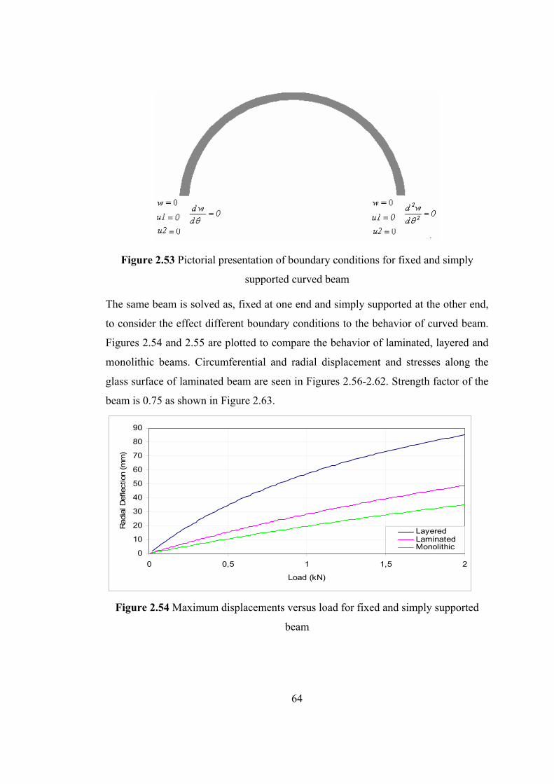
64
Figure 2.53 Pictorial presentation of boundary conditions for fixed and simply
supported curved beam
The same beam is solved as, fixed at one end and simply supported at the other end,
to consider the effect different boundary conditions to the behavior of curved beam.
Figures 2.54 and 2.55 are plotted to compare the behavior of laminated, layered and
monolithic beams. Circumferential and radial displacement and stresses along the
glass surface of laminated beam are seen in Figures 2.56-2.62. Strength factor of the
beam is 0.75 as shown in Figure 2.63.
0
10
20
30
40
50
60
70
80
90
0 0,5 1 1,5 2
Load (kN)
Rad
ial D
efle
ctio
n (m
m)
LayeredLaminatedMonolithic
Figure 2.54 Maximum displacements versus load for fixed and simply supported
beam
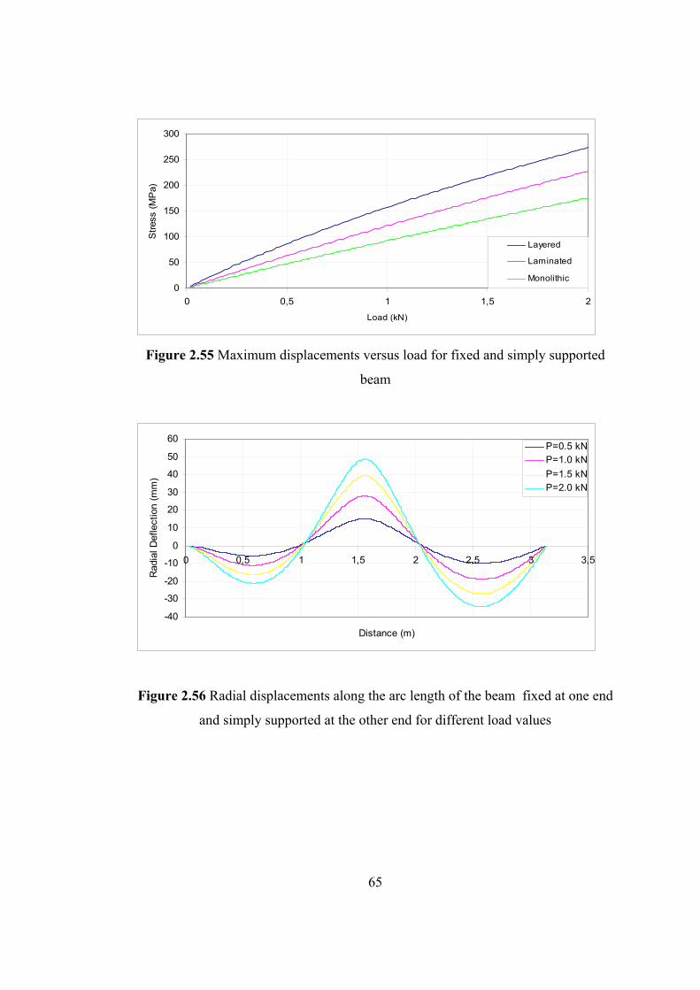
65
0
50
100
150
200
250
300
0 0,5 1 1,5 2
Load (kN)
Str
ess
(MP
a)
Layered
Laminated
Monolithic
Figure 2.55 Maximum displacements versus load for fixed and simply supported
beam
-40
-30
-20
-10
0
10
20
30
40
50
60
0 0,5 1 1,5 2 2,5 3 3,5
Distance (m)
Rad
ial D
efle
ctio
n (m
m)
P=0.5 kNP=1.0 kN
P=1.5 kNP=2.0 kN
Figure 2.56 Radial displacements along the arc length of the beam fixed at one end
and simply supported at the other end for different load values
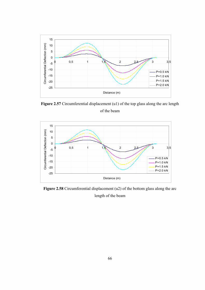
66
-25
-20
-15
-10
-5
0
5
10
15
0 0,5 1 1,5 2 2,5 3 3,5
Distance (m)
Circ
umfe
rent
ial D
efle
ctio
n (m
m)
P=0.5 kN
P=1.0 kN
P=1.5 kN
P=2.0 kN
Figure 2.57 Circumferential displacement (u1) of the top glass along the arc length
of the beam
-25
-20
-15
-10
-5
0
5
10
15
0 0,5 1 1,5 2 2,5 3 3,5
Distance (m)
Circ
umfe
rent
ial D
efle
ctio
n (m
m)
P=0.5 kN
P=1.0 kN
P=1.5 kNP=2.0 kN
Figure 2.58 Circumferential displacement (u2) of the bottom glass along the arc
length of the beam
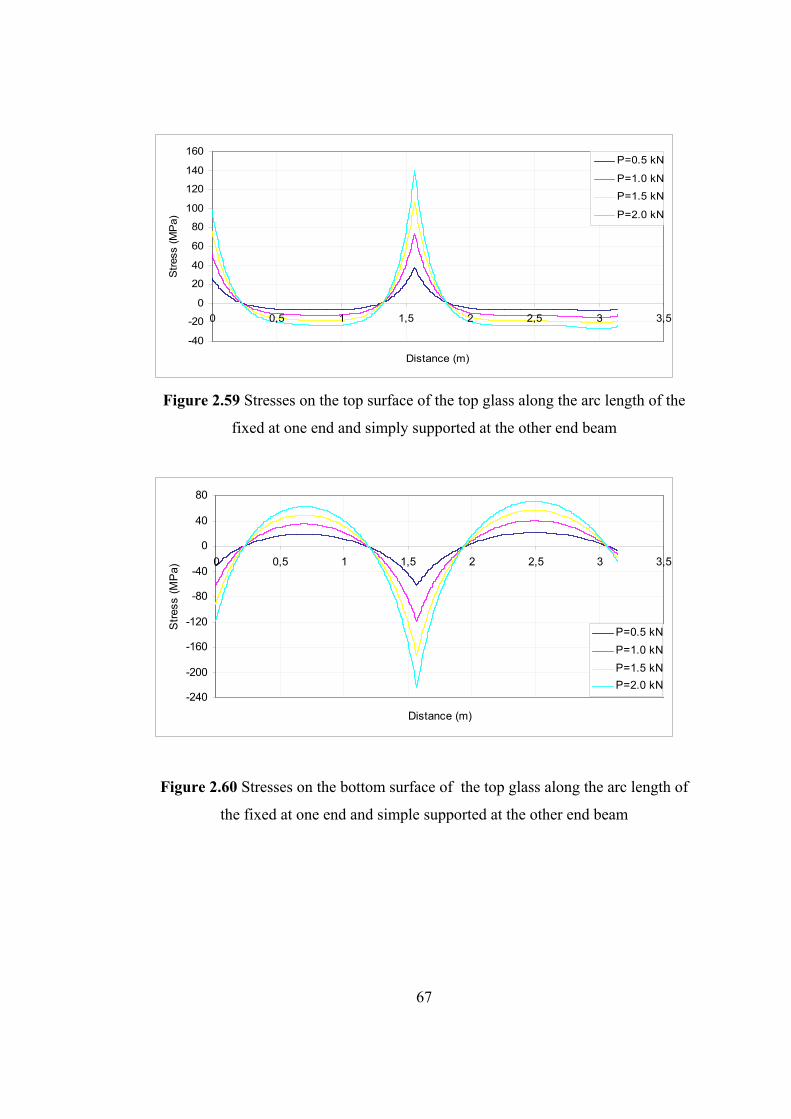
67
-40
-20
0
20
40
60
80
100
120
140
160
0 0,5 1 1,5 2 2,5 3 3,5
Distance (m)
Str
ess
(MP
a)P=0.5 kN
P=1.0 kN
P=1.5 kN
P=2.0 kN
Figure 2.59 Stresses on the top surface of the top glass along the arc length of the
fixed at one end and simply supported at the other end beam
-240
-200
-160
-120
-80
-40
0
40
80
0 0,5 1 1,5 2 2,5 3 3,5
Distance (m)
Str
ess
(MP
a)
P=0.5 kN
P=1.0 kN
P=1.5 kN
P=2.0 kN
Figure 2.60 Stresses on the bottom surface of the top glass along the arc length of
the fixed at one end and simple supported at the other end beam
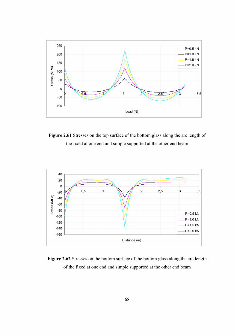
68
-100
-50
0
50
100
150
200
250
0 0,5 1 1,5 2 2,5 3 3,5
Load (N)
Str
ess
(MP
a)P=0.5 kN
P=1.0 kN
P=1.5 kN
P=2.0 kN
Figure 2.61 Stresses on the top surface of the bottom glass along the arc length of
the fixed at one end and simple supported at the other end beam
-160
-140
-120
-100
-80
-60
-40
-20
0
20
40
0 0,5 1 1,5 2 2,5 3 3,5
Distance (m)
Str
ess
(MP
a)
P=0.5 kN
P=1.0 kN
P=1.5 kN
P=2.0 kN
Figure 2.62 Stresses on the bottom surface of the bottom glass along the arc length
of the fixed at one end and simple supported at the other end beam
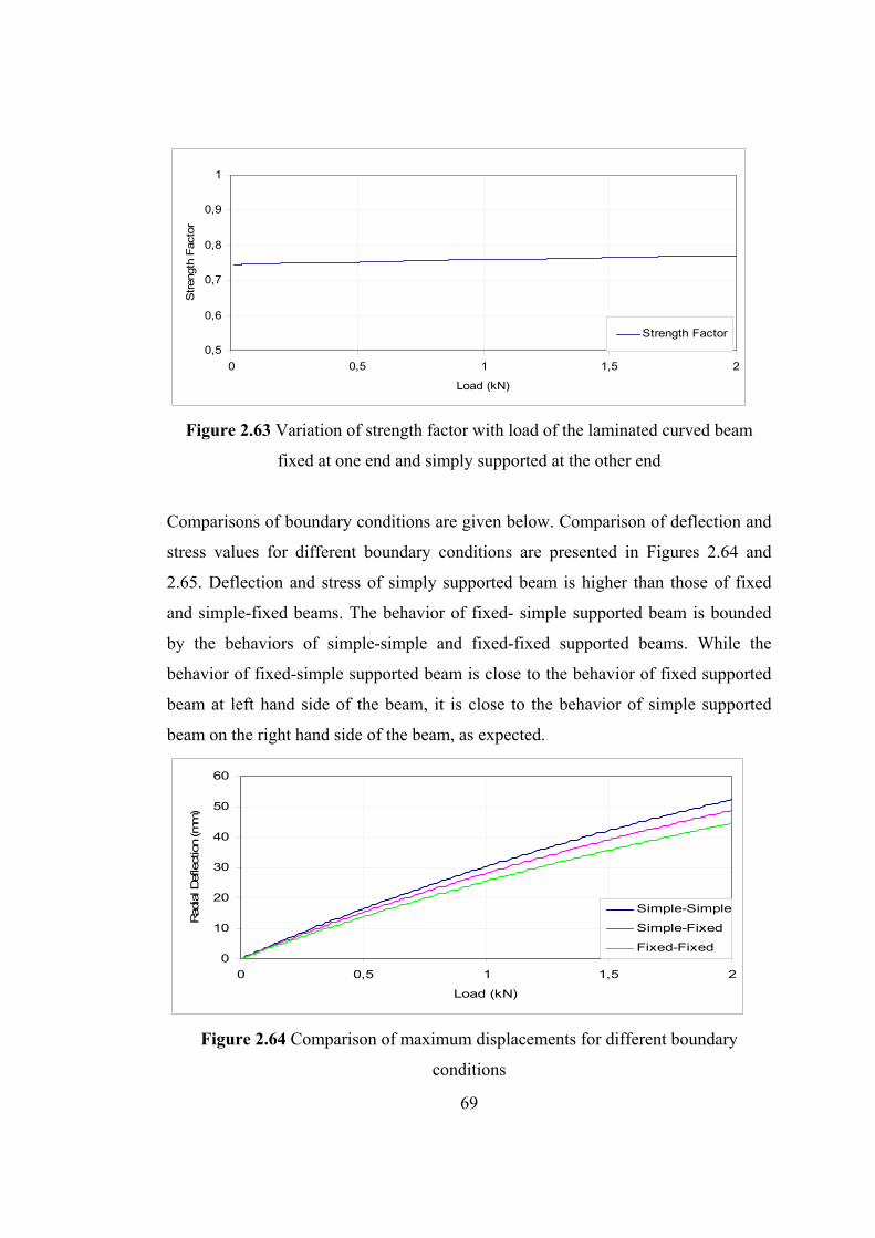
69
0,5
0,6
0,7
0,8
0,9
1
0 0,5 1 1,5 2
Load (kN)
Stren
gth
Fac
tor
Strength Factor
Figure 2.63 Variation of strength factor with load of the laminated curved beam
fixed at one end and simply supported at the other end
Comparisons of boundary conditions are given below. Comparison of deflection and
stress values for different boundary conditions are presented in Figures 2.64 and
2.65. Deflection and stress of simply supported beam is higher than those of fixed
and simple-fixed beams. The behavior of fixed- simple supported beam is bounded
by the behaviors of simple-simple and fixed-fixed supported beams. While the
behavior of fixed-simple supported beam is close to the behavior of fixed supported
beam at left hand side of the beam, it is close to the behavior of simple supported
beam on the right hand side of the beam, as expected.
0
10
20
30
40
50
60
0 0,5 1 1,5 2
Load (kN)
Rad
ial D
efle
ctio
n (m
m)
Simple-Simple
Simple-Fixed
Fixed-Fixed
Figure 2.64 Comparison of maximum displacements for different boundary
conditions
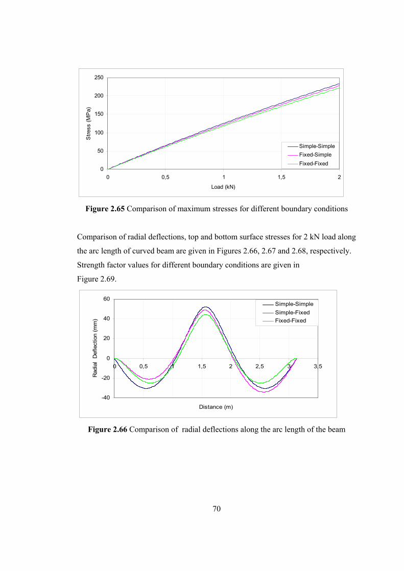
70
0
50
100
150
200
250
0 0,5 1 1,5 2
Load (kN)
Str
ess
(MP
a)
Simple-Simple
Fixed-Simple
Fixed-Fixed
Figure 2.65 Comparison of maximum stresses for different boundary conditions
Comparison of radial deflections, top and bottom surface stresses for 2 kN load along
the arc length of curved beam are given in Figures 2.66, 2.67 and 2.68, respectively.
Strength factor values for different boundary conditions are given in
Figure 2.69.
-40
-20
0
20
40
60
0 0,5 1 1,5 2 2,5 3 3,5
Distance (m)
Rad
ial
Def
lect
ion
(mm
)
Simple-Simple
Simple-Fixed
Fixed-Fixed
Figure 2.66 Comparison of radial deflections along the arc length of the beam
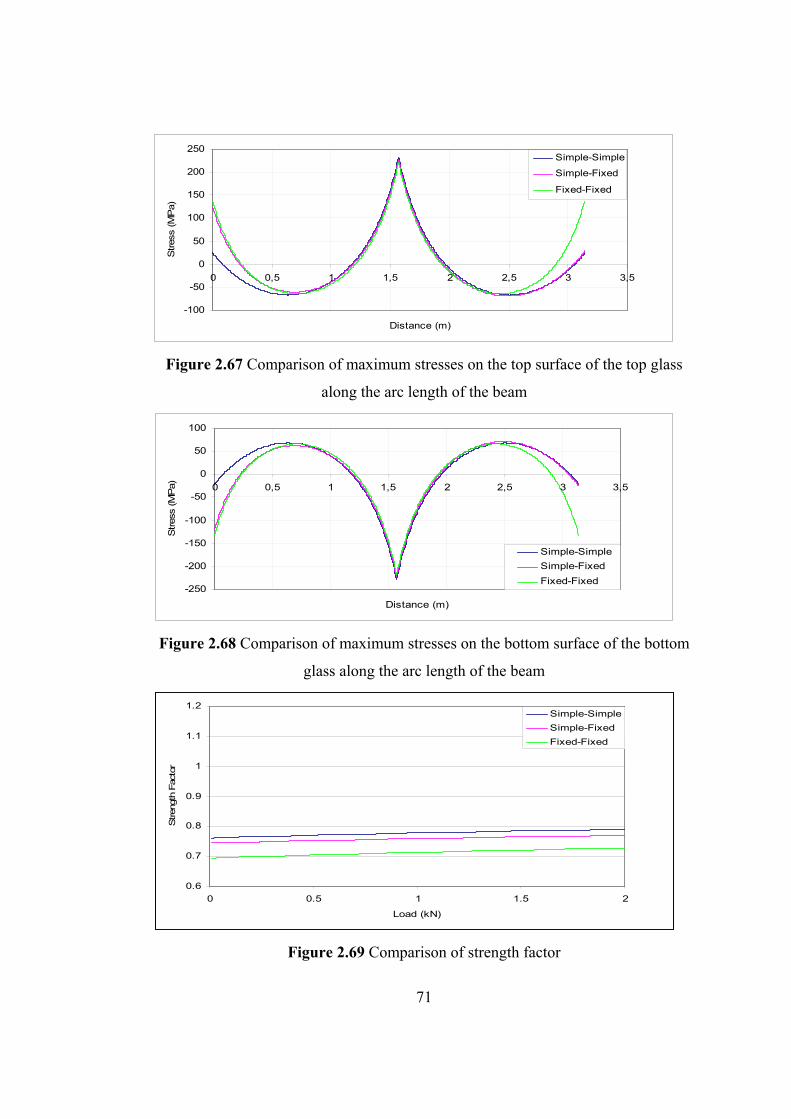
71
-100
-50
0
50
100
150
200
250
0 0,5 1 1,5 2 2,5 3 3,5
Distance (m)
Stres
s (M
Pa)
Simple-Simple
Simple-Fixed
Fixed-Fixed
Figure 2.67 Comparison of maximum stresses on the top surface of the top glass
along the arc length of the beam
-250
-200
-150
-100
-50
0
50
100
0 0,5 1 1,5 2 2,5 3 3,5
Distance (m)
Stres
s (M
Pa)
Simple-Simple
Simple-Fixed
Fixed-Fixed
Figure 2.68 Comparison of maximum stresses on the bottom surface of the bottom
glass along the arc length of the beam
0.6
0.7
0.8
0.9
1
1.1
1.2
0 0.5 1 1.5 2
Load (kN)
Stren
gth
Fac
tor
Simple-Simple
Simple-Fixed
Fixed-Fixed
Figure 2.69 Comparison of strength factor
72
2.6 Summary and Conclusion
A mathematical model with nonlinear partial differential equations and a numerical
solution technique are developed to predict the linear and nonlinear behavior of a
laminated glass curved beam. Governing nonlinear coupled differential equations
involving circumferential displacements u1 and u2 and radial displacement w are
derived by using minimum potential energy theorem and variational approach. To
develop nonlinear model and to obtain field and boundary equations large deflection
theory is used. In the numerical solution of the nonlinear partial differential
equations convergence difficulties are faced and to overcome these convergence
difficulties variable SOR (here is named as SUR: Successive Under Relaxation)
parameter is used. It also needs higher number of divisions and tolerance value than
those for straight beams. Model is verified by test results conducted by Uzhan [27] in
the mechanics laboratory of the Department of Engineering Sciences and by
generating and solving a commercial finite element program. The comparison of
results obtained from the current theoretical model, finite element model and
experiments on laminated glass curved beam are matching quite well.
The developed model simulates the layered and monolithic glass cases successfully.
Although the behavior of a laminated glass curved beam is bounded by the behavior
of monolithic and layered curved glass beams these bounds are violated at some parts
of the beam along its arc length, which is not the case in the behavior of straight
beams. On the other hand, the behavior of a curved laminated glass beam depends on
the shear modulus of interlayer PVB. It is possible to make the laminated glass arch
stronger than the monolithic glass arch by increasing the shear modulus of interlayer.
The present model provides valuable insight to the general behavior of laminated
glass curved beam. The effect of PVB’s shear modulus, the level of nonlinearity,
displacement, moment and stress functions are observed. To consider the effect of
boundary conditions to the behavior of curved beam the model is solved for different
boundary conditions. The results are compared in figures. Nonlinearity level of
simply supported beam is found to be higher than that of fixed supported beam.
73
Strength factor, which is employed to adjust laminated strengths by using available
design charts, is obtained for curved beams. Strength factor of fixed supported
laminated curved beam is found to be higher than that of simply supported beam.
While strength factor of simply supported curved beam is nearly 0.8, strength factor
of fixed supported curved beam is nearly 0.7.
74
CHAPTER 3
BEHAVIOR OF LAMINATED GLASS CYLINDRICAL
SHELLS
3.1 Introduction to Theory of Shells
Shell structures are load carrying elements which have a great importance in
engineering and in particular, in civil, mechanical, architectural and marine
engineering. Large span roofs, water tanks, concrete arch domes, liquid retaining
structures are examples of shell structures. A shell is said to be a curved structural
element whose thickness is small when compared with the other dimensions of shell
and with its radius of the curvature. Examples of the shell structures include pipes,
pressure vessels, roofs, dooms, sheds, airplane wings, car sheds, turbine disks and
bulkheads. Mid surface of the shell can be defined as the plane bisecting the shell
thickness. To describe the shape of the shell we specify the geometry of middle
surface and the thickness of the shell at each point.
When thickness of the shell is one-twentieth of radius of curvature or less they are
defined as thin otherwise they are defined as thick shells.
To analyze the shell structures, equations of elasticity, membrane and bending theory
are applied. Membrane forces are obtained for the given loading and then
superimposed on the bending theory for edge loads. The solution procedure of shell
is based on the following Love shell theory assumptions:
1- the shell is thin,
2- the displacement and rotations are small,
3- the normal shell datum surface before deformation remains normal after
deformation,
75
4- the transverse normal stress is negligible.
The above assumptions are often called Kirchhoff-Love shell theory, which is an
extension of Kirchhoff flat-plate theory.
3.2 Nonlinear Behavior of Shells
In the general case, nonlinearities are present when describing the response of a solid
body. There are two types of nonlinearities due to material and geometry. Material
nonlinearity is a result of changing material properties with the applied loads or
force-displacement or stress-strain law, which is not linear.
Geometric nonlinearity is a result of nonlinear kinematic quantities such as the
strain- displacement relations. Large strains, large displacements and large rotations
can cause geometric nonlinearity.
The lateral deflection of the shell is not small when compared with the thickness of
the shell. For this reason the mid-plane of the shell, develop stresses and the
differential equations become nonlinear.
The geometry of a cylindrical glass shell unit may be layered, laminated or
monolithic.
Layered glass consists of two glass sheets with no friction between them. Stress
distribution of each ply is symmetric with respect to their individual neutral axis. The
glass sheets share the load equally. ‘Plane sections before deformation remain plane
after deformation’ assumption is not valid for layered glass units because curvature
centers of plies are different.
Monolithic glass consists of one glass sheet. Stress distribution of monolithic glasses
is symmetric around the neutral axis of the glass unit. Because of single center of
curvature, ‘plane sections remain plane’ assumption is valid for monolithic glass
units.
Laminated glass consists of two or more glass sheets connected with an interlayer.
Stress distribution of laminated glass is the summation of constant coupling stress of
interlayer and the two triangular stress distribution of a layered beam, which is
76
symmetrical about the neutral axes of each ply. The size of coupling stress is
depending on the shear modulus of the interlayer. While coupling stress is
compressive at the top ply, it is tensile at the bottom ply.
3.3 Mathematical Model for Laminated Glass Shell Unit
Laminated glass unit consists of two thin glass shells and an interlayer placed in
between the glass sheets. The behavior of laminated glass unit which is subjected to
the radial pressures is highly nonlinear since the maximum value of radial
displacement in the units becomes larger than the thickness of it and shear modulus
of the interlayer is very small when compared with that of the glass shell. The effect
of nonlinear behavior is considered in the derivation of the field equations and
boundary conditions. Because of nonlinearity, the classic assumption that ‘plane
section before deformation remains plane after deformation’ is no longer valid. For
this reason, the existing theories can not be employed satisfactorily and a more
realistic new model is needed. Therefore, a new nonlinear shell theory has been
developed for the analysis of laminated glass shells by using minimum potential
energy theorem. The minimum potential energy theorem is a possible tool to obtain
the field equations and boundary conditions for the considered problem.
For mathematical modeling of glass shells, the following assumptions are made:
1. The shell material is completely homogenous and isotropic.
2. The material of the shell is elastic and obeys Hooke ’s law.
3. Because of small thickness of the shell shear deformation is ignored.
4. Normal to the mid-plane of the shell before deformation remains normal after
deformation.
5. For nonlinear behavior, in-plane displacement derivatives are so small that the
higher powers of the in-plane displacement derivatives and values of their product
are ignored.
6. For nonlinear behavior, membrane stresses are developed in the mid-plane, but are
still small when compared with the other shell dimensions. This causes the mid-plane
to be stretched under the effect of radial loads.
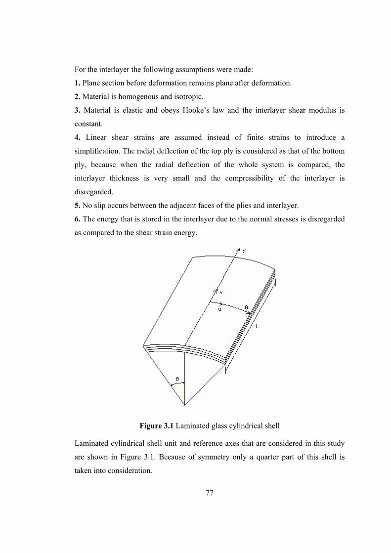
77
For the interlayer the following assumptions were made:
1. Plane section before deformation remains plane after deformation.
2. Material is homogenous and isotropic.
3. Material is elastic and obeys Hooke’s law and the interlayer shear modulus is
constant.
4. Linear shear strains are assumed instead of finite strains to introduce a
simplification. The radial deflection of the top ply is considered as that of the bottom
ply, because when the radial deflection of the whole system is compared, the
interlayer thickness is very small and the compressibility of the interlayer is
disregarded.
5. No slip occurs between the adjacent faces of the plies and interlayer.
6. The energy that is stored in the interlayer due to the normal stresses is disregarded
as compared to the shear strain energy.
Figure 3.1 Laminated glass cylindrical shell
Laminated cylindrical shell unit and reference axes that are considered in this study
are shown in Figure 3.1. Because of symmetry only a quarter part of this shell is
taken into consideration.
78
Using the above assumptions, which are given for glass layers and interlayer, the
total potential energy Π of the system, can be written as:
VUΠ
ΩUUUUUUΠ Ir
Iyr
2b
1b
2m
1m (3.1)
where,
1mU , 2
mU = membrane strain energy for the top and bottom shells, respectively,
1bU , 2
bU = bending strain energy for the top and bottom shells, respectively,
Ir
Iyr U,U = shear strain energy of the interlayer in y-r and r-θ planes, respectively,
= potential energy function due to applied loads.
According to Langhaar (1962), the bending strain energy functions are given as:
1
1
a
a
2y1y11
2y1
212
1311
b dyd)))(2
1())((2)()(
)1(24
rEhU
(3.2)
1
1
a
a
2y2y22
2y2
222
2322
b dyd)))(2
1())((2)()(
)1(24
rEhU
(3.3)
In the above equation 1 , y1 , y1 and 2 , y2 , y2 are the bending strains for the
top and bottom shells, respectively and they can be expressed as follows:
79
21
1 r
w 2
22 r
w
yyy1 w yyy2 w
y1
y1 wr
2
y2
y2 wr
2
The membrane strain energy functions can be expressed in terms of strains and they
are given as follows:
(3.4)
(3.5)
where,
1 , y1 , y1 and 2 , y2 , y2 are the nonlinear membrane strains and for
the top and bottom shell units, respectively.They can be expressed in terms of the
displacement as follows:
2yyy1 w2
11v
1
y
1yy1 r
ww
r
1v1u
dyd)))(2
1())((2)()(
)1(2
rEhU
1
1
a
a
2y1y11
2y1
21
2111
m
2
111 r
w
2
1
r
w1u
dyd)))(2
1())((2)()(
)1(2
rEhU
1
1
a
a
2y2y22
2y2
22
2222
m
2
222 r
w
2
1
r
w2u
2yyy2 w2
12v
2
y
2yy2 r
ww
r
2v2u
80
The average shear strains r and yr are obtained from Figure 2.2 which is plotted to
show deformed and undeformed sections of the shell unit
r
r
uwr
t/]2
h
r
1
2
h
r
1(
w2u1u[
w)
r
1( 2
2
1
1Ir
yyyr
r
v
y
wyr
t/]2
h
2
h(
y
w2v1v[
y
w 21yr
Making use of the shear strain equations, interlayer shear strain energy expressions
are written as:
t
)w
)r
t
2
h
r
1
2
h
r
1(2u1u(
I
2
2
1
1r
t
)y
w)t
2
h
2
h(2v1v( 21
yr
81
(3.6)
(3.7)
This problem has a uniformly distributed load and the load potential function can be
written as:
1
1
a
a
1 dydqwr
(3.8)
where,
i = 1, 2 denotes the top and bottom shells, respectively,
E = Young modulus of the glass shells,
G = interlayer shear modulus,
ih = thickness of the shell,
ir = radius of the shell,
= Poisson’s ratio of the glass,
Ir = radius of the interlayer,
t = thickness of the interlayer,
w = radial deflection of laminated glass unit for the top and bottom shell,
1u , 2u = circumferential displacements of top and bottom glass shells, respectively.
1v , 2v = axial displacements of top and bottom glass shells, respectively
dyd]t
)w
)r
t
2
h
r
1
2
h
r
1(2u1u(
[2
GtrU 2I
2
2
1
11
1
a
a
IIr
dyd]t
)y
w)t
2
h
2
h(2v1v(
[2
GtrU 2
211
1
a
a
IIyr
dVGUt a
a
rIr
0
21
12
1
dVGUt a
a
yrIyr
0
21
12
1
82
The total potential energy of the system is written by substituting the Equations
(3.2), (3.3), (3.4), (3.5), (3.7) and (3.8) into Equation (3.1).
dV)UUUUUU( Ir
Iyr
2b
1b
2m
1m
v
1
1
a
a
dyFtrd
Here F can be expressed as:
Minimum potential energy theorem, which states that corresponding to the
satisfaction of stable equilibrium of all geometric possible configurations of a body is
identified by minimum value for the potential energy, and variational approach are
used to solve this problem. The total potential energy of the system is written respect
to the radial and in plane displacements 1u , 2u , 1v , 2v and w. Euler Equation which
is given by Langhaar (1962), is applied to the total potential energy to obtain the
governing differential equations of the system.
1y2
22
2
yy22
22
32
2y2y22
2y2
22
22
2y1y11
2y1
21
11
y1
yy21
2
yy21
21
31
21
I
2
2
1
1
I
qwr2
wr
2
2
1yy
wr
w22w
2
r
w
)21(24
rEh
2
)1(2
)21(2
rEh
2
)1(2
)21(2
rEh
2w
r
2
2
1w
r
w22w
2
r
w
)21(24
rEh
2)y
w)t
2
h
2
h(2v1v(2)
w)
r
t
2
h
r
1
2
h
r
1(2u1u(
t2
GrF
83
Euler Equation in its most general form is:
0ui
F
yui
F
yui
F
ui
F
yui
F
u
F
yy2
2
y
2
2
2
yi
where,
ui denotes 1u , 2u , 1v , 2v and w respectively,
ui is the first derivative of ui with respect to θ,
yui is the first derivative of ui with respect to y,
ui is the second derivative of ui with respect to θ,
yyui is the second derivative of ui with respect to y,
yui is the second order cross derivative of ui .
Mathematical calculations give the following five nonlinear governing equations of
laminated glass shell unit, which are obtained with respect to radial and in-plane
displacement:
(3.9)
(3.10)
0)w
r
t
2
h
r
1
2
h
r
12u1u(
tr
Gr2N
r
1
y
)2N(
I
2
2
1
12
I
2
y
0)w
r
t
2
h
r
1
2
h
r
12u1u(
tr
Gr1N
r
1
y
)1N(
I
2
2
1
11
I
1
y
84
(3.11)
(3.12)
(3.13)
where,
0y
wt
2
h
2
h2v1v
tr
Gr
y
1N)1N(
r
1 21
1
Iyy
1
0y
wt
2
h
2
h2v1v
tr
Gr
y
2N)2N(
r
1 21
2
Iyy
2
0w
r
1
y
w
r
2
y
wr
112
Eh
w
r
1
y
w
r
2
y
wr
112
Eh
w
r
t
2
h
r
1
2
h
r
12u1u
r
1
r
1
t
Gr
w
r
t
2
h
r
1
2
h
r
12u1u
r
t
2
h
r
1
2
h
r
1
t
Gr
y
wt
2
h
2
h
y
2v
y
1vt
2
h
2
h
t
Gr
y
w2N21N2
w
r
2N
r
1N
y
wr2Nr1N1N1Nqr
4
4
32
22
4
24
4
22
32
4
4
31
22
4
14
4
12
31
I
2
2
1
121
I
2
2
I
2
2
1
1I
2
2
1
1
I
2
22121I
2
yy
2
2
212
2
2y1y1
)y11
()21(
1Eh
1N
)1y1
()21(
1Eh
y1N
)()1(2
Eh1N y1
1y
)y22
()21(
2Eh
2N
)2y2
()21(
2Eh
y2N
)()1(2
Eh2N y2
2y
85
The governing equations in extended form are as follows.
)r2
ν1(
y
2v)
r2
ν1(
y
w
y
w
y
w
2r2
ν)1(
θ
w
r
1
r
1w
)θ
w
r
t
2
h
r
1
2
h
r
11(u
trEh
)ν1(Gr2)u
trEh
)ν1(Gr
y2
ν1
θr
1(
2
2
2
2
2
2
2
2
32
22
I
2
2
1
122
2I
22
2I
2
2
2
2
22
)r2
ν1(
y
1u)
r2
ν1(
y
www
r2
ν)1(
y
w
ry
w
)y
wt
2
h
2
h2v(
trEh
)ν1(Gr1)v
trEh
)ν1(Gr
r2
ν1
y(
1
2
21
2
2
2
21
2
2
1
21
11
2I
11
2I
2
2
22
2
1
)r2
ν1(
y
2u)
r2
ν1(
y
www
r2
ν)1(
y
w
ry
w
)y
wt
2
h
2
h1(v
trEh
)ν1(Gr2)v
trEh
)ν1(Gr
r2
ν1
y(
2
2
22
2
2
2
22
2
2
2
2
11
2I
22
2I
2
2
22
2
2
1
)r2
ν1(
y
1v)
r2
ν1(
y
w
y
w)
θ
w
r
t
2
h
r
1
2
h
r
12u(
trEh
)ν1(Gr
y
w
r2
ν)1(
θ
w
r
1
r
1w1)u
trEh
)ν1(Gr
y2
ν1
θr
1(
1
2
1
2
I
2
2
1
111
2I
2
2
12
2
31
2111
2I
2
2
2
2
21
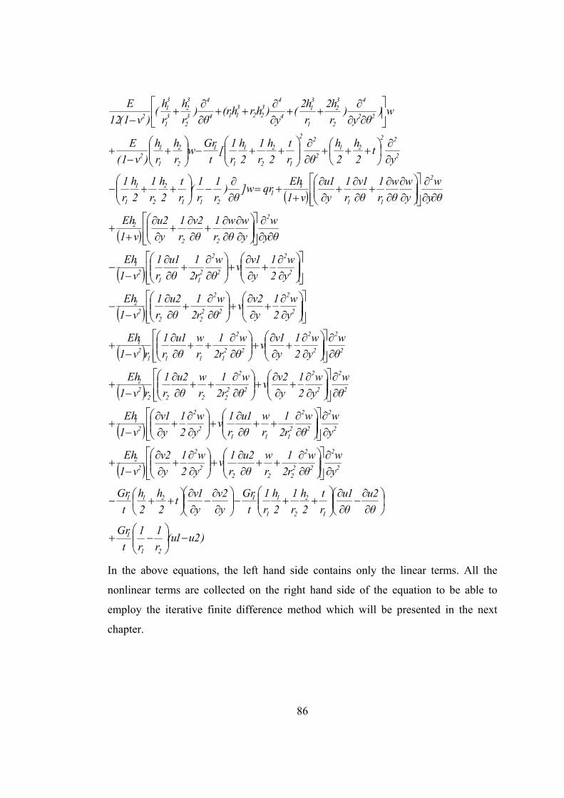
86
)2u1(ur
1
r
1
t
Gr
θ
2u
θ
1u
r
t
2
h
r
1
2
h
r
1
t
Gr
y
2v
y
1vt
2
h
2
h
t
Gr
y
w
θ
w
r2
1
r
w
θ
2u
r
1ν
y
w
2
1
y
2v
ν1
Eh
y
w
θ
w
r2
1
r
w
θ
1u
r
1ν
y
w
2
1
y
1v
ν1
Eh
θ
w
y
w
2
1
y
2vν
θ
w
r2
1
r
w
θ
2u
r
1
rν1
Eh
θ
w
y
w
2
1
y
1vν
θ
w
r2
1
r
w
θ
1u
r
1
rν1
Eh
y
w
2
1
y
2vν
θ
w
r2
1
θ
2u
r
1
ν1
Eh
y
w
2
1
y
1vν
θ
w
r2
1
θ
1u
r
1
ν1
Eh
θy
w
y
w
θ
w
r
1
θ
2v
r
1
y
2u
ν1
Eh
θy
w
y
w
θ
w
r
1
θ
1v
r
1
y
1u
ν1
Ehqr]w
θ)
r
1
r
1(
r
t
2
h
r
1
2
h
r
1
yt
2
h
2
h
θr
t
2
h
r
1
2
h
r
1[
t
Grw
r
h
r
h
)ν1(
E
w)θy
)r
h2
r
h2(
y)hrh(r
θ)
r
h
r
h(
)ν1(12
E
21
I
I
2
2
1
1
I21I
2
2
2
2
2222
2
2
22
2
2
2
2
2111
2
2
21
2
2
2
2
2
2
22222
22
2
2
2
2
2
2
21111
21
2
2
2
2
222
22
2
2
2
2
211
21
2
22
2
2
11
11
21I
2
2
1
1
2
22
212
22
I
2
2
1
1
I
2
2
1
12
22
4
2
32
1
31
4
4322
3114
4
32
32
31
31
2
In the above equations, the left hand side contains only the linear terms. All the
nonlinear terms are collected on the right hand side of the equation to be able to
employ the iterative finite difference method which will be presented in the next
chapter.
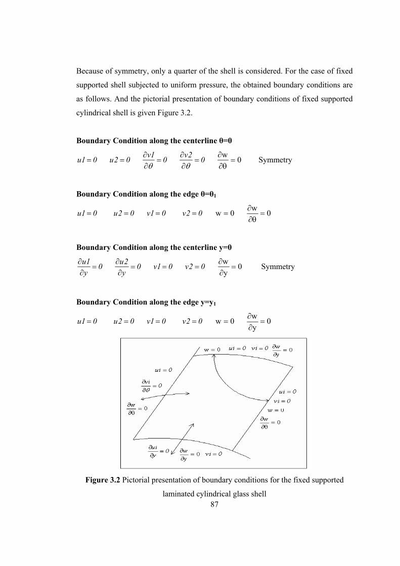
87
Because of symmetry, only a quarter of the shell is considered. For the case of fixed
supported shell subjected to uniform pressure, the obtained boundary conditions are
as follows. And the pictorial presentation of boundary conditions of fixed supported
cylindrical shell is given Figure 3.2.
Boundary Condition along the centerline θ=0
01u 02u 01v
02v
0w
Symmetry
Boundary Condition along the edge θ=θ1
01u 02u 01v 02v 0w 0w
Boundary Condition along the centerline y=0
0y
1u
0y
2u
01v 02v 0y
w
Symmetry
Boundary Condition along the edge y=y1
01u 02u 01v 02v 0w 0y
w
Figure 3.2 Pictorial presentation of boundary conditions for the fixed supported
laminated cylindrical glass shell
88
3.4 Finite Difference Expressions for Field and Boundary Equations
and The Iterative Solution Technique
3.4.1 Application of Finite Difference Method (FDM)
Due to symmetry of geometry only one quarter of the shell is considered in the
analysis. The governing differential equations of laminated glass shell unit are given
in Equations 3.7 through 3.11. It is found that the differential equations of u1, u2, v1
and v2 are linear while the field equation for radial displacement , w, is nonlinear.
Close form solution of these nonlinear governing differential equations is not known.
Therefore, to solve the equations an iterative technique has to be adopted.
Finite difference method is used to convert the governing differential equations into
discrete values of u1, u2, v1, v2 and w at every point of the finite difference mesh.
Nonlinear partial differential equations are arranged in such a way that the left-hand
side of the governing equations becomes linear; all the nonlinear terms are collected
on the right hand side of the equality. The equations in the matrix form are obtained
for radial and in-plane displacements. While full coefficient matrices are obtained for
in-plane displacements, symmetric banded coefficient matrix is obtained for radial
displacement. Because of the large memory necessity, the modified strongly implicit
procedure, which was proposed by Schneider and Zedan (1981) is employed for the
in plane displacements.
The algebraic equations for the radial displacement are stored in matrix A. Therefore,
the system of equation can be written as:
)2v,1v,2u,1u,w(fqwA 1
where,
w = the radial displacement vector,
q= applied pressure magnitude,
[A] = coefficient matrix for radial displacement.
89
[A] is symmetric and banded coefficient matrix, and the elements are stored in
banded forms. The right-hand side vector includes applied load and the other terms
calculated at every point inside the domain.
In this chapter, the coefficient matrices, and the corresponding right-hand side
vectors inside the domain as well as those at the boundaries are presented. For the
radial deflection, the finite difference mesh size is chosen to be nθ x ny, where nθ and
ny being the number of subdivisions in the θ and y directions, respectively. The size
of coefficient matrix A is (nθny, 2nθ+1). In order to reduce the total number of
equations the radial deflection value at the fixed supported edges which is zero, is not
incorporated. Finite difference expression for radial deflection field equation inside
the domain is:
For i=3,4,...nθ-2, j=3,4,...ny-2
(3.14)
where,
2
I
2
2
1
12
I
2
212y
I
2
2
1
12
2
32
1
31
2y
2232
32
31
31
424y
22
321
31
r
t
2
h
r
1
2
h
r
1
th
Gr2t
2
h
2
h
th
Gr2
r
h
r
h
1
E
r
h
r
h
hh16
E4
r
h
r
h
h12
E
h12
rhrhEC
2
212y
I
2
32
1
31
2y
224y
22
321
31 t
2
h
2
h
th
Gr
r
h
r
h
hh112
E4
h112
rhrhE4J
4
y2
2321
31
h112
rhrhEG
32
32
31
31
42112 r
h
r
h
h
EH
j,i1j,1i1j,1i1j,1i1j,1i2j,i
2j,i1j,i1j,ij,2ij,2ij,1ij,1ij,i
RHSFwFwFwFwGw
GwJwJwHwHwBwBwCw
90
I
2
2
1
121
I
2
I
2
2
1
12I
2
32
1
31
2y
2232
32
31
31
42
r
t
2
h
r
1
2
h
r
1
r
1
r
1
th2
Gr_
r
t
2
h
r
1
2
h
r
1
th
Gr
r
h
r
h
hh112
E4
r
h
r
h
h112
E4B
2
32
1
31
2y
22 r
h
r
h
hh16
EF
121
I
21I
I
2
2
1
1
I
2
2
2
2
222
22
2
2
2
2
211
21
2
θy22
2
θ2y222
2
y2θ22
22
2
θy12
2
θ1y112
2
y1θ11
21
i,j
qr2u1ur
1
r
1
t
Gr
y
2v
y
1vt
2
h
2
h
t
Gr_
2u1u
r
t
2
h
r
1
2
h
r
1
t
Gr
y
w
2
1
y
2vν
θ
w
r2
1
θ
2u
r
1
ν1
Eh
y
w
2
1
y
1vν
θ
w
r2
1
θ
1u
r
1
ν1
Eh
yθ
wν1
y
wνr
wν
r
1
ν1
Eh
yθ
wν1
y
wνr
θ
wν
r
1
ν1
EhRHS
The general equation is modified at the shell boundaries and the following equations
are obtained for fixed supported shell:
For i=1, j=1
422224,
1,12,1,,2,1,ji
jijijijijiji
RHSFww
Gw
Jw
Hw
Bw
C
91
For i=1, j=2
22222,
1,11,12,1,1,,2,1,ji
jijijijijijijiji
RHSFwFww
Gw
Jw
JHwBww
GC
For i=1, j=3,4,...ny-1
2
RHSFw
Fww2
Gw
2
Gw
2
Jw
2
JHwBww
2
C
j,i1j,1i
1j,1i2j,i2j,i1j,i1j,ij,2ij,1ij,i
For i=1, j=ny
2222,
1,12,1,,2,1,ji
jijijijijiji
RHSFww
Gw
JHwBww
GC
For i=2, j=1
22222,
1,11,11,2,,1,2,1,ji
jijijijijijijiji
RHSFwFwJwGww
Bw
Hw
Bw
HC
For i=2, j=2
jijiji
jijijijijijijijiji
RHSFwFw
FwFwGwJwJwHwBwBwwHGC
,1,11,1
1,11,12,1,1,,2,1,1,)(
For i=2, j=3,4,....ny-2
jijiji
jijijijijijijijijiji
RHSFwFw
FwFwGwGwJwJwHwBwBwwHC
,1,11,1
1,11,12,2,1,1,,2,1,1,)(
92
For i=2, j=ny-1
jijiji
jijijijijijijijiji
RHSFwFw
FwFwGwJwJwHwBwBwwHC
,1,11,1
1,11,12,1,1,,2,1,1,)(
For i=2, j=ny
jijijijijijijijiji RHSFwFwGwJwHwBwBwwHGC ,1,11,12,1,,2,1,1,)(
For i=3,4.… .nθ-2, j=1
222222,
1,11,12,1,,2,2,1,1,
ji
jijijijijijijijiji
RHSFwFwGwJww
Hw
Hw
Bw
Bw
C
For i=nθ-1, j=1
22222,
1,11,12,1,,2,1,1,ji
jijijijijijijiji
RHSFwFwGwJww
Hw
Bw
Bw
C
For i=nθ-1, j=3,4...ny-2
j,i1j,1i1j,1i
1j,1i1j,1i2j,i2j,i1j,i1j,ij,2ij,1ij,1ij,i
RHSFwFw
FwFwGwGwJwJwHwBwBwCw
For i=nθ, j=3,4,...ny-2
j,i1j,1i
1j,1i2j,i2j,i1j,i1j,ij,2ij,1ij,i
RHSFw
FwGwGwJwJwHwBww)HC(
For i=nθ, j=ny-1
jijijijijijijijiji RHSFwFwGwJwJwHwBwwHC ,1,11,12,1,1,,2,1,)(
93
For i=nθ, j=1
2
RHSFwGwJww
2
Hw
2
Bw)
2
HC( j,i
1j,1i2j,i1j,ij,2ij,1ij,i
For i=nθ-1, j=2
j,i1j,1i!j,1i1j,1i
1j,1i2j,i1j,i1j,ij,2ij,1ij,1ij,i
RHSFwFwFw
FwGwJwJwHwBwBww)GC(
For i=nθ, j=2
j,i1j,1i
1j,1i2j,i1j,i1j,ij,2ij,1ij,i
RHSFw
FwGwJwJwHwBww)HGC(
For i=nθ, j=ny
jijijijijijiji RHSFwGwJwHwBwwHGC ,1,12,1,,2,1,)(
For i=nθ-1, j=ny-1
jijiji
jijijijijijijijiji
RHSFwFw
FwFwGwJwJwHwBwBwCw
,1,11,1
1,11,12,1,1,,2,1,1,
For i=3,4,...nθ-2, j=2
j,i1j,1i1j,1i1j,1i1j,1i
2j,i1j,i1j,ij,2ij,2ij,1ij,1ij,i
RHSFwFwFwFw
GwJwJwHwHwBwBww)GC(
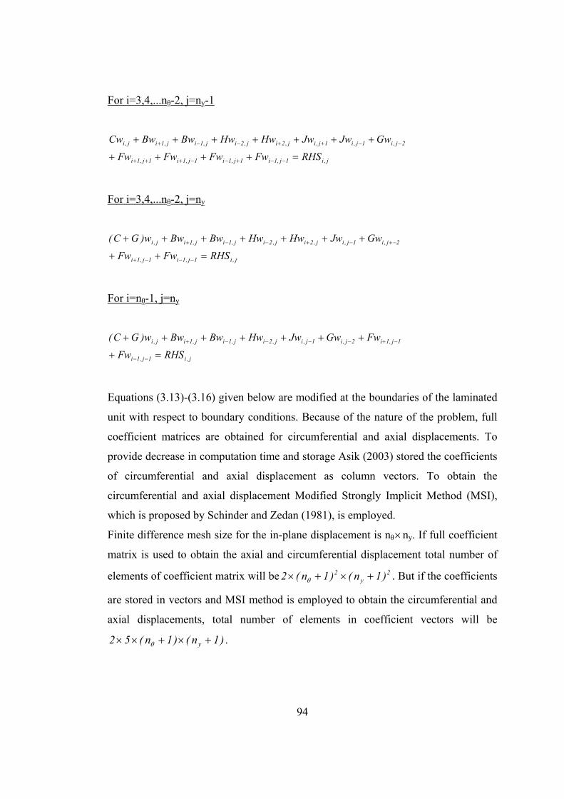
94
For i=3,4,...nθ-2, j=ny-1
j,i1j,1i1j,1i1j,1i1j,1i
2j,i1j,i1j,ij,2ij,2ij,1ij,1ij,i
RHSFwFwFwFw
GwJwJwHwHwBwBwCw
For i=3,4,...nθ-2, j=ny
j,i1j,1i1j,1i
2j,i1j,ij,2ij,2ij,1ij,1ij,i
RHSFwFw
GwJwHwHwBwBww)GC(
For i=nθ-1, j=ny
j,i1j,1i
1j,1i2j,i1j,ij,2ij,1ij,1ij,i
RHSFw
FwGwJwHwBwBww)GC(
Equations (3.13)-(3.16) given below are modified at the boundaries of the laminated
unit with respect to boundary conditions. Because of the nature of the problem, full
coefficient matrices are obtained for circumferential and axial displacements. To
provide decrease in computation time and storage Asik (2003) stored the coefficients
of circumferential and axial displacement as column vectors. To obtain the
circumferential and axial displacement Modified Strongly Implicit Method (MSI),
which is proposed by Schinder and Zedan (1981), is employed.
Finite difference mesh size for the in-plane displacement is nθny. If full coefficient
matrix is used to obtain the axial and circumferential displacement total number of
elements of coefficient matrix will be 2y
2 )1n()1n(2 . But if the coefficients
are stored in vectors and MSI method is employed to obtain the circumferential and
axial displacements, total number of elements in coefficient vectors will be
)1n()1n(52 y .
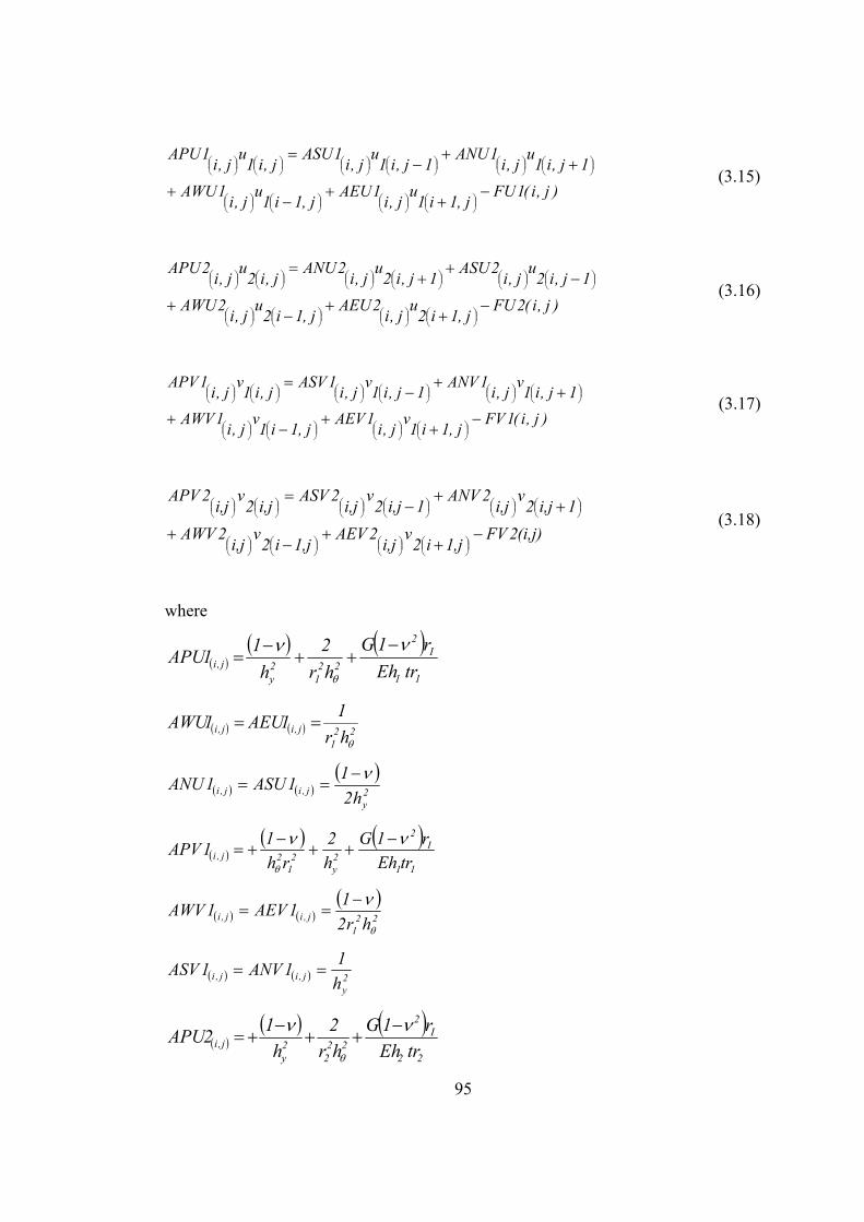
95
)j,i(1FUj,1i1
uj,i
1AEUj,1i1
uj,i
1AWU
1j,i1u
j,i1ANU
1j,i1u
j,i1ASU
j,i1u
j,i1APU
(3.15)
)j,i(2FUj,1i2
uj,i
2AEUj,1i2
uj,i
2AWU
1j,i2u
j,i2ASU
1j,i2u
j,i2ANU
j,i2u
j,i2APU
(3.16)
)j,i(1FVj,1i1
vj,i
1AEVj,1i1
vj,i
1AWV
1j,i1v
j,i1ANV
1j,i1v
j,i1ASV
j,i1v
j,i1APV
(3.17)
(i,j)2FV,j1i2
vi,j
2AEV,j1i2
vi,j
2AWV
1i,j2v
i,j2ANV
1i,j2v
i,j2ASV
i,j2v
i,j2APV
(3.18)
where
11
I2
221
2y
j,i trEh
r1G
hr
2
h
11APU
221
j,ij,ihr
11AEU1AWU
2y
j,ij,i h2
11ASU1ANU
11
I2
2y
21
2j,i trEh
r1G
h
2
rh
11APV
221
j,ij,i hr2
11AEV1AWV
2y
j,ij,i h
11ANV1ASV
22
I2
222
2y
j,i trEh
r1G
hr
2
h
12APU
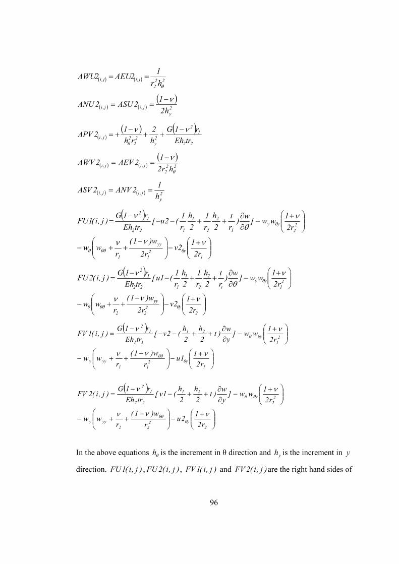
96
222
j,ij,ihr
12AEU2AWU
2y
j,ij,i h2
12ASU2ANU
22
I2
2y
22
2j,i trEh
r1G
h
2
rh
12APV
222
j,ij,i hr2
12AEV2AWV
2y
j,ij,i h
12ANV2ASV
1y2
1
yy
1
22
yyI
2
2
1
122
I2
r2
12v
r2
w)1(
rww
r2
1ww]
w)
r
t
2
h
r
1
2
h
r
1(2u[
trEh
r1G)j,i(1FU
2y2
2
yy
2
21
yyı
2
2
1
122
I2
r2
12v
r2
w)1(
rww
r2
1ww]
w)
r
t
2
h
r
1
2
h
r
1(1u[
trEh
r1G)j,i(2FU
1y2
11yyy
21
y21
11
I2
r2
11u
r
w)1(
rww
r2
1ww]
y
w)t
2
h
2
h(2v[
trEh
r1G)j,i(1FV
2y2
22yyy
22
y21
22
I2
r2
12u
r
w)1(
rww
r2
1ww]
y
w)t
2
h
2
h(1v[
trEh
r1G)j,i(2FV
In the above equations h is the increment in θ direction and yh is the increment in y
direction. )j,i(1FU , )j,i(2FU , )j,i(1FV and )j,i(2FV are the right hand sides of
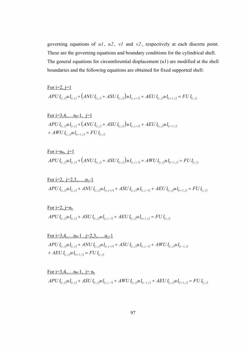
97
governing equations of 1u , 2u , 1v and 2v , respectively at each discrete point.
These are the governing equations and boundary conditions for the cylindrical shell.
The general equations for circumferential displacement (u1) are modified at the shell
boundaries and the following equations are obtained for fixed supported shell:
For i=2, j=1
j,ij,1ij,i1j,ij,ij,ij,ij,i 1FU1u1AEU1u1ASU1ANU1u1APU
For i=3,4,.…nθ-1, j=1
j,ij,1ij,i
j,1ij,i1j,ij,ij,ij,ij,i
1FU1u1AWU
1u1AEU1u1ASU1ANU1u1APU
For i=nθ, j=1
j,ij,1ij,i1j,ij,ij,ij,ij,i 1FU1u1AWU1u1ASU1ANU1u1APU
For i=2, j=2,3,.….ny-1
j,ij,1ij,i1j,ij,i1j,ij,ij,ij,i 1FU1u1AEU1u1ASU1u1ANU1u1APU
For i=2, j=ny
j,ij,1ij,i1j,ij,ij,ij,i 1FU1u1AEU1u1ASU1u1APU
For i=3,4,.…nθ-1 . j=2,3,.….ny-1
j,ij,1ij,i
j,1ij,i1j,ij,i1j,ij,ij,ij,i
1FU1u1AEU
1u1AWU1u1ASU1u1ANU1u1APU
For i=3,4,.…nθ-1, j= ny
j,ij,1ij,ij,1ij,i1j,ij,ij,ij,i 1FU1u1AEU1u1AWU1u1ASU1u1APU
98
For i=nθ, j=2,3,.….ny-1
j,ij,1ij,i1j,ij,i1j,ij,ij,ij,i 1FU1u1AWU1u1ASU1u1ANU1u1APU
For i=nθ, j=ny
j,ij,1ij,i1j,ij,ij,ij,i 1FU1u1AWU1u1ASU1u1APU
The general equations for circumferential displacement (u2) are obtained for fixed
supported shell as follows:
For i=2, j=1
j,ij,1ij,i1j,ij,ij,ij,ij,i 2FU2u2AEU2u2ASU2ANU2u2APU
For i=3,4,.…nθ-1, j=1
j,ij,1ij,i
j,1ij,i1j,ij,ij,ij,ij,i
2FU2u2AWU
2u2AEU2u2ASU2ANU2u2APU
For i=nθ, j=1
j,ij,1ij,i1j,ij,ij,ij,ij,i 2FU2u2AWU2u2ASU2ANU2u2APU
For i=2, j=2,3,.….ny-1
j,ij,1ij,i1j,ij,i1j,ij,ij,ij,i 2FU2u2AEU2u2ASU2u2ANU2u2APU
For i=2, j=ny
j,ij,1ij,i1j,ij,ij,ij,i 2FU2u2AEU2u2ASU2u2APU
For i=3,4,.…nθ-1 . j=2,3,.….ny-1
j,ij,1ij,i
j,1ij,i1j,ij,i1j,ij,ij,ij,i
2FU2u2AEU
2u2AWU2u2ASU2u2ANU2u2APU
99
For i=3,4,.…nθ-1, j= ny
j,ij,1ij,ij,1ij,i1j,ij,ij,ij,i 2FU2u2AEU2u2AWU2u2ASU2u2APU
For i=nθ, j=2,3,.….ny-1
j,ij,1ij,i1j,ij,i1j,ij,ij,ij,i 2FU2u2AWU2u2ASU2u2ANU2u2APU
For i=nθ, j=ny
j,ij,1ij,i1j,ij,ij,ij,i 2FU2u2AWU2u2ASU2u2APU
Modified axial displacement (v1) at the shell boundaries are obtained for fixed
supported shell as follows:
For i=1, j=2
j,ij,1ij,ij,i1j,ij,ij,ij,i 1FV1v1AWV1AEV1v1ANV1v1APV
For i=2,3,.…nθ-1, j=2
j,ij,1ij,ij,1ij,i1j,ij,ij,ij,i 1FV1v1AEV1v1AWV1v1ANV1v1APV
For i=nθ, j=2
j,ij,1ij,i1j,ij,ij,ij,i 1FV1v1AWV1v1ANV1v1APV
For i=1, j=3,4,.….ny-1
j,i
j,1ij,ij,i1j,ij,i1j,ij,ij,ij,i
1FV
1v1AWV1AEV1v1ANV1v1ASV1v1APV
For i=1, j=ny
j,ij,1ij,ij,i1j,ij,ij,ij,i 1FV1v1AWV1AEV1v1ASV1v1APV
100
For i=2,3,.…nθ-1, j=3,4,.….ny-1
j,ij,1ij,i
j,1ij,i1j,ij,i1j,ij,ij,ij,i
1FV1v1AEV
1v1AWV1v1ANV1v1ASV1v1APV
For i=2,3,.…nθ-1, j=ny
j,ij,1ij,ij,1ij,i1j,ij,ij,ij,i 1FV1v1AEV1v1AWV1v1ASV1v1APV
For i=nθ, j=3,4,.….ny-1
j,ij,1ij,i1j,ij,i1j,ij,ij,ij,i 1FV1v2AWV1v2ANV1v1ASV1v1APV
For i=nθ, j=ny
j,ij,1ij,i1j,ij,ij,ij,i 1FV1v1AWV1v1ASV1v1APV
Modified axial displacement (v2) at the shell boundaries are obtained for fixed
supported shell as follows:
For i=1, j=2
j,ij,1ij,ij,i1j,ij,ij,ij,i 2FV2v2AWV2AEV2v2ANV2v2APV
For i=2,3,.…nθ-1, j=2
j,ij,1ij,ij,1ij,i1j,ij,ij,ij,i 2FV2v2AEV2v2AWV2v2ANV2v2APV
For i=nθ, j=2
j,ij,1ij,i1j,ij,ij,ij,i 2FV2v2AWV2v2ANV2v2APV
For i=1, j=3.4.….ny-1
j,i
j,1ij,ij,i1j,ij,i1j,ij,ij,ij,i
2FV
2v2AWV2AEV2v2ANV2v2ASV2v2APV
101
For i=1, j=ny
j,ij,1ij,ij,i1j,ij,ij,ij,i 2FV2v2AWV2AEV2v2ASV2v2APV
For i=2,3,.…nθ-1, j=3,4,.….ny-1
j,ij,1ij,i
j,1ij,i1j,ij,i1j,ij,ij,ij,i
2FV2v2AEV
2v2AWV2v2ANV2v2ASV2v2APV
For i=2,3,.…nθ-1, j=ny
j,ij,1ij,ij,1ij,i1j,ij,ij,ij,i 2FV2v2AEV2v2AWV2v2ASV2v2APV
For i=nθ, j=3,4,.….ny-1
j,ij,1ij,i1j,ij,i1j,ij,ij,ij,i 2FV2v2AWV2v2ANV2v2ASV2v2APV
For i=nθ, j=ny
j,ij,1ij,i1j,ij,ij,ij,i 2FV2v2AWV2v2ASV2v2APV
3.4.2 Solution Algorithm Using finite difference method, governing differential equations 3.7 through 3.11 are
converted into algebraic equations at every point of the domain. The equations are
obtained in matrix form as:
)k(
)i(1)k()i( )2v,1v,2u,1u,w(fqwA (3.19)
In above equations w denotes the radial displacement vector while U denotes the
in-plane displacement vector for u1, u2, v1, v2and q designates the applied pressure.
Subscripts (i) denote the iteration number while superscripts (k) designate the
increment number.
Coefficient matrice [A] is linear while the right hand side vectors f1 is nonlinear. To
transform nonlinear algebraic equations into the set of quasi linear equations the
values of w, u1, u2, v1 and v2 from the (i-1)th iteration are put into right hand side of
equation 3.17 of the ith iteration. Value of radial displacement w for i th iteration is
102
obtained from equation 3.17. The new value of radial displacement is used to
calculate the right hand side of equation of equation of u1, u2, v1 and v2. Then
equations are solved to obtain u1, v1, and v2. The solution procedure is repeated
until convergence is achieved.
The steps of an iterative procedure are listed below:
1. assume w, u1, u2, v1, v2,
2. calculate RHS of governing equation for the radial displacement,
3. obtain w(i.j) from
RwA
4. recalculate ),,()1(),(),( 0 jiwjiwjiw
where is under relaxation parameter. This parameter is used in order to overcome
convergence difficulties. is calculated by interpolation regarding the non-
dimensional maximum displacement )/(*2 21)1,1( hhw as a result of numerical
experiment and ),(0 jiw is the radial displacement that is calculated in the previous
step. Radial displacement w is interpolated by using
h
wmax and in-plane
displacement is extrapolated by using 4.1
5. if
tolwnum
wwji
jioji
max
,,,
* then stop the iteration,
6. calculate )j,i(1FU and 1u from governing equation of 1u ,
7. calculate )j,i(2FU and 2u from governing equation of 2u ,
8. calculate )j,i(1FV and 1v from governing equation of 1v ,
9. calculate )j,i(2FV and 2v from governing equation of 2v ,
10. back to step 2.
The described iterative procedure is implemented by developing a computer code,
which is written in FORTRAN.
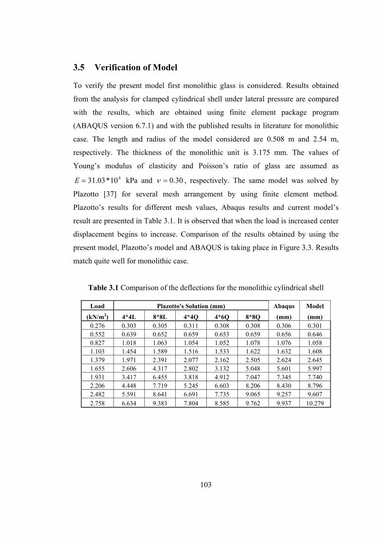
103
3.5 Verification of Model To verify the present model first monolithic glass is considered. Results obtained
from the analysis for clamped cylindrical shell under lateral pressure are compared
with the results, which are obtained using finite element package program
(ABAQUS version 6.7.1) and with the published results in literature for monolithic
case. The length and radius of the model considered are 0.508 m and 2.54 m,
respectively. The thickness of the monolithic unit is 3.175 mm. The values of
Young’s modulus of elasticity and Poisson’s ratio of glass are assumed as
410*03.31E kPa and 30.0 , respectively. The same model was solved by
Plazotto [37] for several mesh arrangement by using finite element method.
Plazotto’s results for different mesh values, Abaqus results and current model’s
result are presented in Table 3.1. It is observed that when the load is increased center
displacement begins to increase. Comparison of the results obtained by using the
present model, Plazotto’s model and ABAQUS is taking place in Figure 3.3. Results
match quite well for monolithic case.
Table 3.1 Comparison of the deflections for the monolithic cylindrical shell
Load Plazotto's Solution (mm) Abaqus Model
(kN/m2) 4*4L 8*8L 4*4Q 4*6Q 8*8Q (mm) (mm) 0.276 0.303 0.305 0.311 0.308 0.308 0.306 0.301 0.552 0.639 0.652 0.659 0.653 0.659 0.656 0.646 0.827 1.018 1.063 1.054 1.052 1.078 1.076 1.058 1.103 1.454 1.589 1.516 1.533 1.622 1.632 1.608 1.379 1.971 2.391 2.077 2.162 2.505 2.624 2.645 1.655 2.606 4.317 2.802 3.132 5.048 5.601 5.997 1.931 3.417 6.455 3.818 4.912 7.047 7.345 7.740 2.206 4.448 7.719 5.245 6.603 8.206 8.430 8.796 2.482 5.591 8.641 6.691 7.735 9.065 9.257 9.607
2.758 6.634 9.383 7.804 8.585 9.762 9.937 10.279
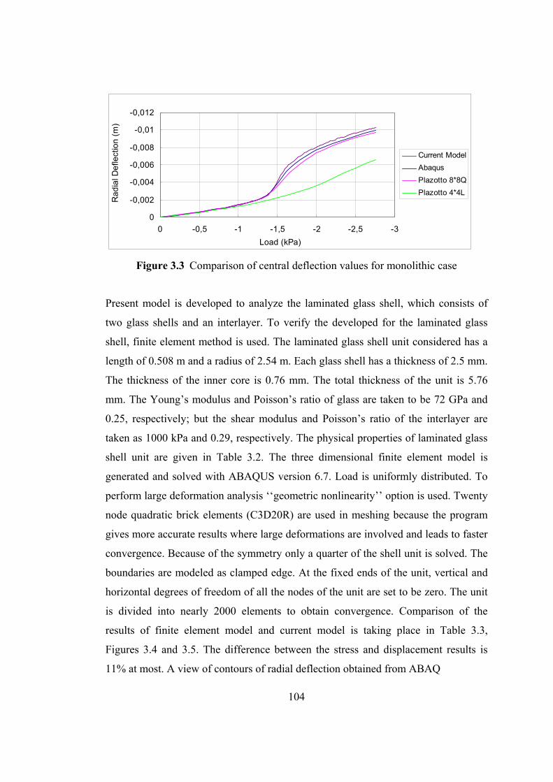
104
-0,012
-0,01
-0,008
-0,006
-0,004
-0,002
0
-3-2,5-2-1,5-1-0,50
Load (kPa)
Ra
dia
l De
flect
ion
(m
)
Current Model
Abaqus
Plazotto 8*8Q
Plazotto 4*4L
Figure 3.3 Comparison of central deflection values for monolithic case
Present model is developed to analyze the laminated glass shell, which consists of
two glass shells and an interlayer. To verify the developed for the laminated glass
shell, finite element method is used. The laminated glass shell unit considered has a
length of 0.508 m and a radius of 2.54 m. Each glass shell has a thickness of 2.5 mm.
The thickness of the inner core is 0.76 mm. The total thickness of the unit is 5.76
mm. The Young’s modulus and Poisson’s ratio of glass are taken to be 72 GPa and
0.25, respectively; but the shear modulus and Poisson’s ratio of the interlayer are
taken as 1000 kPa and 0.29, respectively. The physical properties of laminated glass
shell unit are given in Table 3.2. The three dimensional finite element model is
generated and solved with ABAQUS version 6.7. Load is uniformly distributed. To
perform large deformation analysis ‘‘geometric nonlinearity’’ option is used. Twenty
node quadratic brick elements (C3D20R) are used in meshing because the program
gives more accurate results where large deformations are involved and leads to faster
convergence. Because of the symmetry only a quarter of the shell unit is solved. The
boundaries are modeled as clamped edge. At the fixed ends of the unit, vertical and
horizontal degrees of freedom of all the nodes of the unit are set to be zero. The unit
is divided into nearly 2000 elements to obtain convergence. Comparison of the
results of finite element model and current model is taking place in Table 3.3,
Figures 3.4 and 3.5. The difference between the stress and displacement results is
11% at most. A view of contours of radial deflection obtained from ABAQ
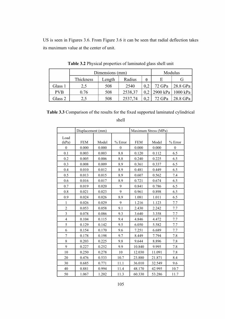
105
US is seen in Figures 3.6. From Figure 3.6 it can be seen that radial deflection takes
its maximum value at the center of unit.
Table 3.2 Physical properties of laminated glass shell unit
Dimensions (mm) Modulus Thickness Length Radius θ E G
Glass 1 2,5 508 2540 0,2 72 GPa 28.8 GPaPVB 0.76 508 2538,37 0,2 2900 kPa 1000 kPa
Glass 2 2,5 508 2537,74 0,2 72 GPa 28.8 GPa
Table 3.3 Comparison of the results for the fixed supported laminated cylindrical
shell
Displacement (mm) Maximum Stress (MPa)
Load (kPa) FEM Model % Error FEM Model % Error
0 0.000 0.000 0 0.000 0.000 0
0.1 0.003 0.003 8.8 0.120 0.112 6.5
0.2 0.005 0.006 8.8 0.240 0.225 6.5
0.3 0.008 0.009 8.9 0.361 0.337 6.5
0.4 0.010 0.012 8.9 0.481 0.449 6.5
0.5 0.013 0.015 8.9 0.607 0.562 7.4
0.6 0.016 0.017 8.9 0.721 0.674 6.5
0.7 0.019 0.020 9 0.841 0.786 6.5
0.8 0.021 0.023 9 0.961 0.898 6.5
0.9 0.024 0.026 8.9 1.081 1.011 6.5
1 0.026 0.029 9 1.216 1.123 7.7
2 0.053 0.058 9.1 2.430 2.242 7.7
3 0.078 0.086 9.3 3.640 3.358 7.7
4 0.104 0.115 9.4 4.846 4.472 7.7
5 0.129 0.142 9.5 6.050 5.582 7.7
6 0.154 0.170 9.6 7.251 6.689 7.7
7 0.178 0.198 9.7 8.449 7.794 7.8
8 0.203 0.225 9.8 9.644 8.896 7.8
9 0.227 0.252 9.9 10.840 9.995 7.8
10 0.250 0.278 10 12.030 11.091 7.8
20 0.476 0.533 10.7 23.880 21.871 8.4
30 0.685 0.771 11.1 36.010 32.549 9.6
40 0.881 0.994 11.4 48.170 42.995 10.7
50 1.067 1.202 11.3 60.330 53.286 11.7
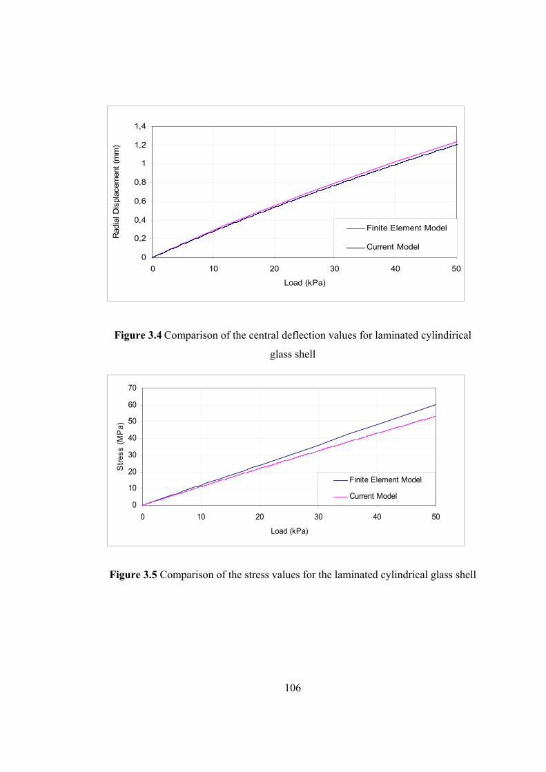
106
0
0,2
0,4
0,6
0,8
1
1,2
1,4
0 10 20 30 40 50
Load (kPa)
Rad
ial D
ispl
acem
ent
(mm
)
Finite Element Model
Current Model
Figure 3.4 Comparison of the central deflection values for laminated cylindirical
glass shell
0
10
20
30
40
50
60
70
0 10 20 30 40 50
Load (kPa)
Str
ess
(MP
a)
Finite Element Model
Current Model
Figure 3.5 Comparison of the stress values for the laminated cylindrical glass shell
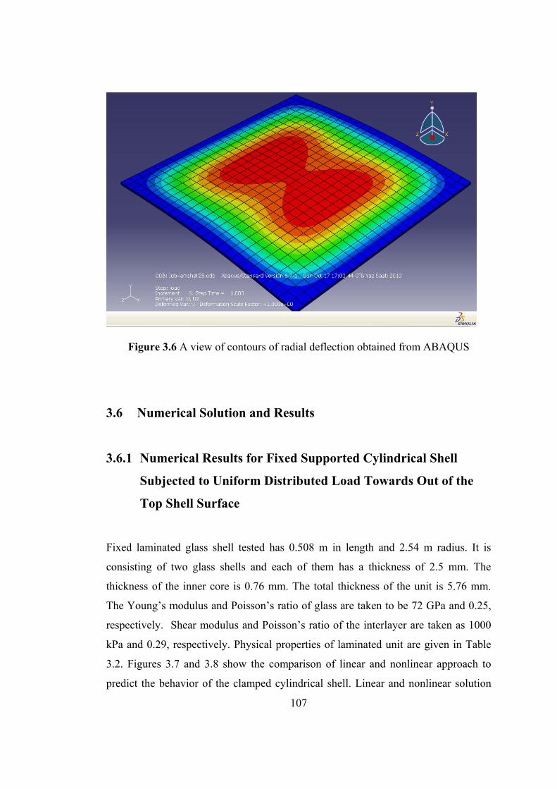
107
Figure 3.6 A view of contours of radial deflection obtained from ABAQUS 3.6 Numerical Solution and Results 3.6.1 Numerical Results for Fixed Supported Cylindrical Shell
Subjected to Uniform Distributed Load Towards Out of the
Top Shell Surface
Fixed laminated glass shell tested has 0.508 m in length and 2.54 m radius. It is
consisting of two glass shells and each of them has a thickness of 2.5 mm. The
thickness of the inner core is 0.76 mm. The total thickness of the unit is 5.76 mm.
The Young’s modulus and Poisson’s ratio of glass are taken to be 72 GPa and 0.25,
respectively. Shear modulus and Poisson’s ratio of the interlayer are taken as 1000
kPa and 0.29, respectively. Physical properties of laminated unit are given in Table
3.2. Figures 3.7 and 3.8 show the comparison of linear and nonlinear approach to
predict the behavior of the clamped cylindrical shell. Linear and nonlinear solution
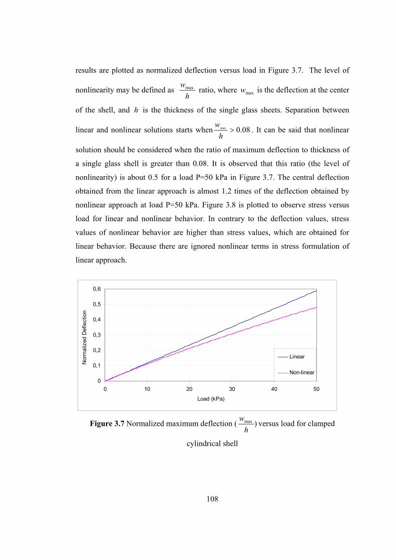
108
results are plotted as normalized deflection versus load in Figure 3.7. The level of
nonlinearity may be defined as h
wmax ratio, where maxw is the deflection at the center
of the shell, and h is the thickness of the single glass sheets. Separation between
linear and nonlinear solutions starts when 08.0max h
w. It can be said that nonlinear
solution should be considered when the ratio of maximum deflection to thickness of
a single glass shell is greater than 0.08. It is observed that this ratio (the level of
nonlinearity) is about 0.5 for a load P=50 kPa in Figure 3.7. The central deflection
obtained from the linear approach is almost 1.2 times of the deflection obtained by
nonlinear approach at load P=50 kPa. Figure 3.8 is plotted to observe stress versus
load for linear and nonlinear behavior. In contrary to the deflection values, stress
values of nonlinear behavior are higher than stress values, which are obtained for
linear behavior. Because there are ignored nonlinear terms in stress formulation of
linear approach.
0
0,1
0,2
0,3
0,4
0,5
0,6
0 10 20 30 40 50
Load (kPa)
Nor
mal
ized
Def
lect
ion
Linear
Non-linear
Figure 3.7 Normalized maximum deflection ( )max
h
wversus load for clamped
cylindrical shell
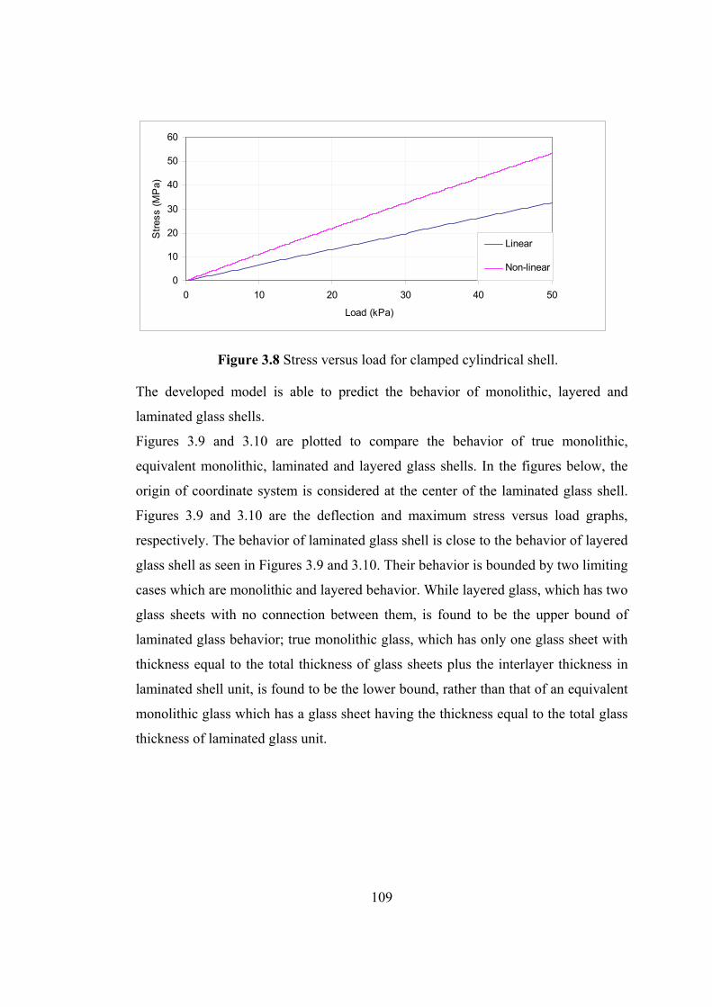
109
0
10
20
30
40
50
60
0 10 20 30 40 50
Load (kPa)
Str
ess
(MP
a)
Linear
Non-linear
Figure 3.8 Stress versus load for clamped cylindrical shell.
The developed model is able to predict the behavior of monolithic, layered and
laminated glass shells.
Figures 3.9 and 3.10 are plotted to compare the behavior of true monolithic,
equivalent monolithic, laminated and layered glass shells. In the figures below, the
origin of coordinate system is considered at the center of the laminated glass shell.
Figures 3.9 and 3.10 are the deflection and maximum stress versus load graphs,
respectively. The behavior of laminated glass shell is close to the behavior of layered
glass shell as seen in Figures 3.9 and 3.10. Their behavior is bounded by two limiting
cases which are monolithic and layered behavior. While layered glass, which has two
glass sheets with no connection between them, is found to be the upper bound of
laminated glass behavior; true monolithic glass, which has only one glass sheet with
thickness equal to the total thickness of glass sheets plus the interlayer thickness in
laminated shell unit, is found to be the lower bound, rather than that of an equivalent
monolithic glass which has a glass sheet having the thickness equal to the total glass
thickness of laminated glass unit.
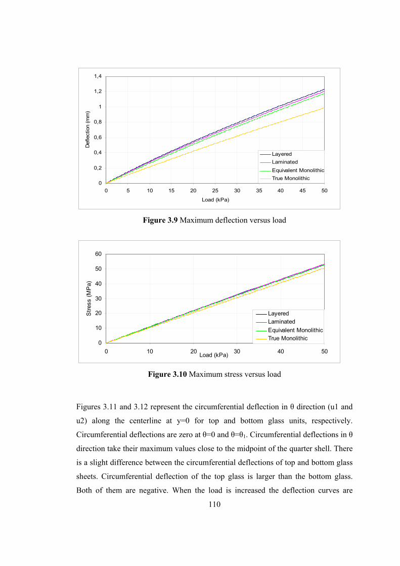
110
0
0,2
0,4
0,6
0,8
1
1,2
1,4
0 5 10 15 20 25 30 35 40 45 50
Load (kPa)
Def
lect
ion
(mm
)
Layered
Laminated
Equivalent Monolithic
True Monolithic
Figure 3.9 Maximum deflection versus load
0
10
20
30
40
50
60
0 10 20 30 40 50Load (kPa)
Str
ess
(MP
a)
LayeredLaminated
Equivalent MonolithicTrue Monolithic
Figure 3.10 Maximum stress versus load
Figures 3.11 and 3.12 represent the circumferential deflection in θ direction (u1 and
u2) along the centerline at y=0 for top and bottom glass units, respectively.
Circumferential deflections are zero at θ=0 and θ=θ1. Circumferential deflections in θ
direction take their maximum values close to the midpoint of the quarter shell. There
is a slight difference between the circumferential deflections of top and bottom glass
sheets. Circumferential deflection of the top glass is larger than the bottom glass.
Both of them are negative. When the load is increased the deflection curves are
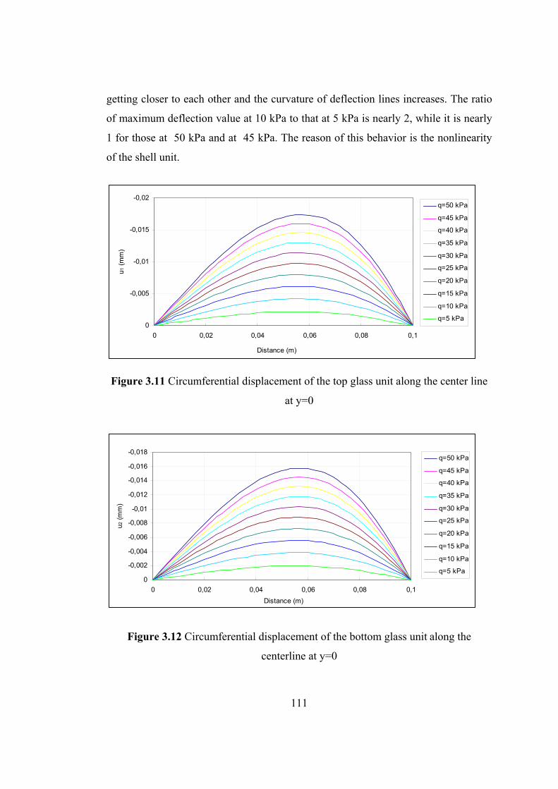
111
getting closer to each other and the curvature of deflection lines increases. The ratio
of maximum deflection value at 10 kPa to that at 5 kPa is nearly 2, while it is nearly
1 for those at 50 kPa and at 45 kPa. The reason of this behavior is the nonlinearity
of the shell unit.
-0,02
-0,015
-0,01
-0,005
0
0 0,02 0,04 0,06 0,08 0,1
Distance (m)
u1 (
mm
)
q=50 kPa
q=45 kPa
q=40 kPa
q=35 kPa
q=30 kPa
q=25 kPa
q=20 kPa
q=15 kPa
q=10 kPa
q=5 kPa
Figure 3.11 Circumferential displacement of the top glass unit along the center line
at y=0
-0,018
-0,016
-0,014
-0,012
-0,01
-0,008
-0,006
-0,004
-0,002
0
0 0,02 0,04 0,06 0,08 0,1
Distance (m)
u2 (
mm
)
q=50 kPa
q=45 kPa
q=40 kPa
q=35 kPa
q=30 kPa
q=25 kPa
q=20 kPa
q=15 kPa
q=10 kPa
q=5 kPa
Figure 3.12 Circumferential displacement of the bottom glass unit along the
centerline at y=0
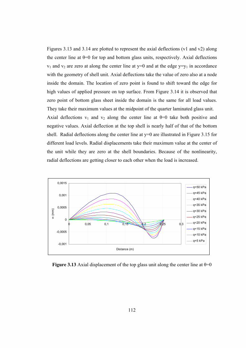
112
Figures 3.13 and 3.14 are plotted to represent the axial deflections (v1 and v2) along
the center line at θ=0 for top and bottom glass units, respectively. Axial deflections
v1 and v2 are zero at along the center line at y=0 and at the edge y=y1 in accordance
with the geometry of shell unit. Axial deflections take the value of zero also at a node
inside the domain. The location of zero point is found to shift toward the edge for
high values of applied pressure on top surface. From Figure 3.14 it is observed that
zero point of bottom glass sheet inside the domain is the same for all load values.
They take their maximum values at the midpoint of the quarter laminated glass unit.
Axial deflections v1 and v2 along the center line at θ=0 take both positive and
negative values. Axial deflection at the top shell is nearly half of that of the bottom
shell. Radial deflections along the center line at y=0 are illustrated in Figure 3.15 for
different load levels. Radial displacements take their maximum value at the center of
the unit while they are zero at the shell boundaries. Because of the nonlinearity,
radial deflections are getting closer to each other when the load is increased.
-0,001
-0,0005
0
0,0005
0,001
0,0015
0 0,05 0,1 0,15 0,2 0,25 0,3
Distance (m)
v1 (
mm
)
q=50 kPa
q=45 kPa
q=40 kPa
q=35 kPa
q=30 kPa
q=25 kPa
q=20 kPa
q=15 kPa
q=10 kPa
q=5 kPa
Figure 3.13 Axial displacement of the top glass unit along the center line at θ=0
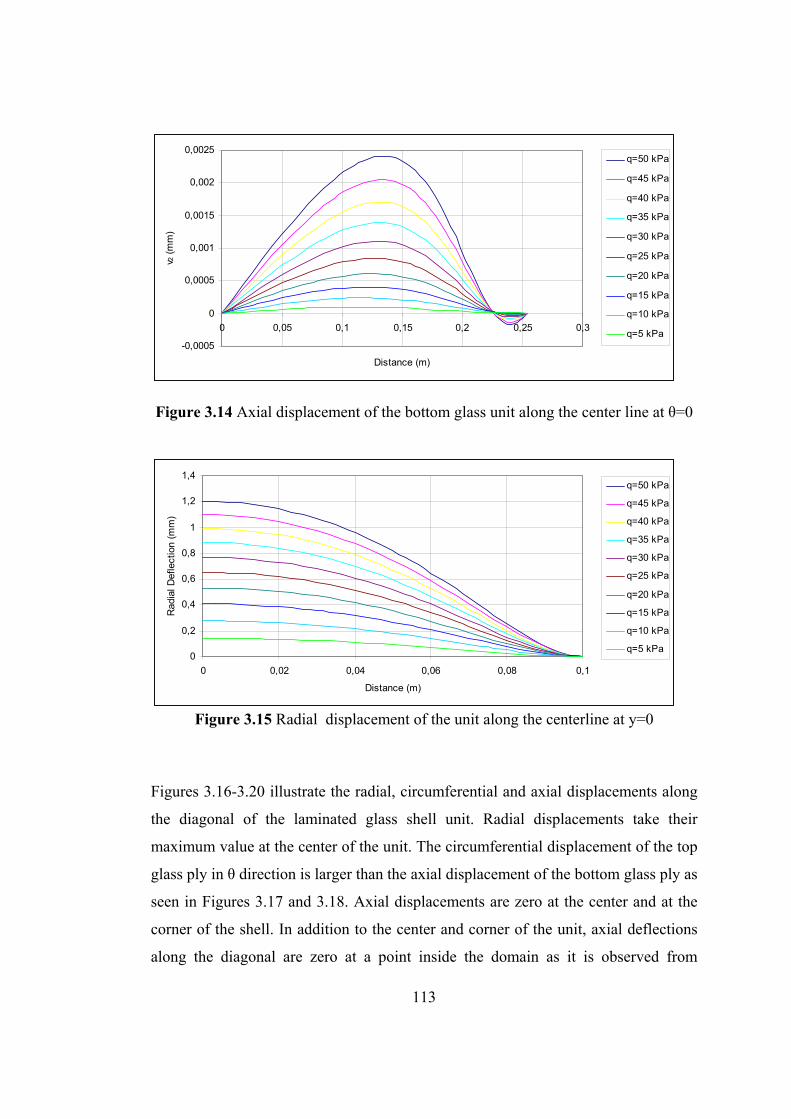
113
-0,0005
0
0,0005
0,001
0,0015
0,002
0,0025
0 0,05 0,1 0,15 0,2 0,25 0,3
Distance (m)
v2 (
mm
)q=50 kPa
q=45 kPa
q=40 kPa
q=35 kPa
q=30 kPa
q=25 kPa
q=20 kPa
q=15 kPa
q=10 kPa
q=5 kPa
Figure 3.14 Axial displacement of the bottom glass unit along the center line at θ=0
0
0,2
0,4
0,6
0,8
1
1,2
1,4
0 0,02 0,04 0,06 0,08 0,1
Distance (m)
Rad
ial D
efle
ctio
n (m
m)
q=50 kPa
q=45 kPa
q=40 kPa
q=35 kPa
q=30 kPa
q=25 kPa
q=20 kPa
q=15 kPa
q=10 kPa
q=5 kPa
Figure 3.15 Radial displacement of the unit along the centerline at y=0
Figures 3.16-3.20 illustrate the radial, circumferential and axial displacements along
the diagonal of the laminated glass shell unit. Radial displacements take their
maximum value at the center of the unit. The circumferential displacement of the top
glass ply in θ direction is larger than the axial displacement of the bottom glass ply as
seen in Figures 3.17 and 3.18. Axial displacements are zero at the center and at the
corner of the shell. In addition to the center and corner of the unit, axial deflections
along the diagonal are zero at a point inside the domain as it is observed from
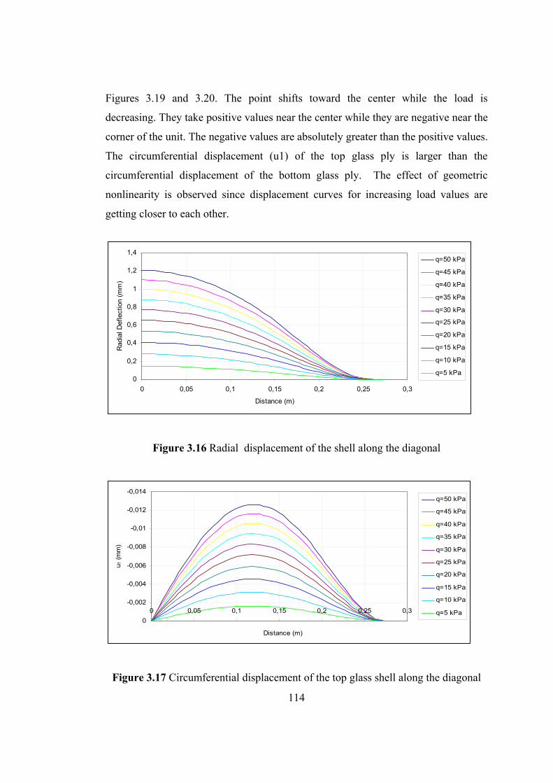
114
Figures 3.19 and 3.20. The point shifts toward the center while the load is
decreasing. They take positive values near the center while they are negative near the
corner of the unit. The negative values are absolutely greater than the positive values.
The circumferential displacement (u1) of the top glass ply is larger than the
circumferential displacement of the bottom glass ply. The effect of geometric
nonlinearity is observed since displacement curves for increasing load values are
getting closer to each other.
0
0,2
0,4
0,6
0,8
1
1,2
1,4
0 0,05 0,1 0,15 0,2 0,25 0,3
Distance (m)
Rad
ial D
efle
ctio
n (m
m)
q=50 kPa
q=45 kPa
q=40 kPa
q=35 kPa
q=30 kPa
q=25 kPa
q=20 kPa
q=15 kPa
q=10 kPa
q=5 kPa
Figure 3.16 Radial displacement of the shell along the diagonal
-0,014
-0,012
-0,01
-0,008
-0,006
-0,004
-0,002
0
0 0,05 0,1 0,15 0,2 0,25 0,3
Distance (m)
u 1 (
mm
)
q=50 kPa
q=45 kPa
q=40 kPa
q=35 kPa
q=30 kPa
q=25 kPa
q=20 kPa
q=15 kPa
q=10 kPa
q=5 kPa
Figure 3.17 Circumferential displacement of the top glass shell along the diagonal
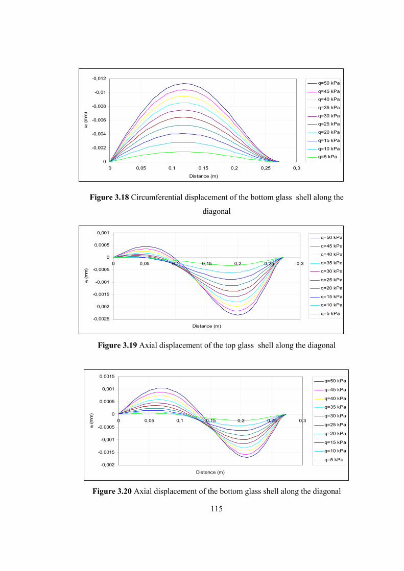
115
-0,012
-0,01
-0,008
-0,006
-0,004
-0,002
0
0 0,05 0,1 0,15 0,2 0,25 0,3
Distance (m)
u 2 (m
m)
q=50 kPa
q=45 kPa
q=40 kPa
q=35 kPa
q=30 kPa
q=25 kPa
q=20 kPa
q=15 kPa
q=10 kPa
q=5 kPa
Figure 3.18 Circumferential displacement of the bottom glass shell along the
diagonal
-0,0025
-0,002
-0,0015
-0,001
-0,0005
0
0,0005
0,001
0 0,05 0,1 0,15 0,2 0,25 0,3
Distance (m)
v 1 (m
m)
q=50 kPa
q=45 kPa
q=40 kPa
q=35 kPa
q=30 kPa
q=25 kPa
q=20 kPa
q=15 kPa
q=10 kPa
q=5 kPa
Figure 3.19 Axial displacement of the top glass shell along the diagonal
-0,002
-0,0015
-0,001
-0,0005
0
0,0005
0,001
0,0015
0 0,05 0,1 0,15 0,2 0,25 0,3
Distance (m)
v 2 (m
m)
q=50 kPa
q=45 kPa
q=40 kPa
q=35 kPa
q=30 kPa
q=25 kPa
q=20 kPa
q=15 kPa
q=10 kPa
q=5 kPa
Figure 3.20 Axial displacement of the bottom glass shell along the diagonal
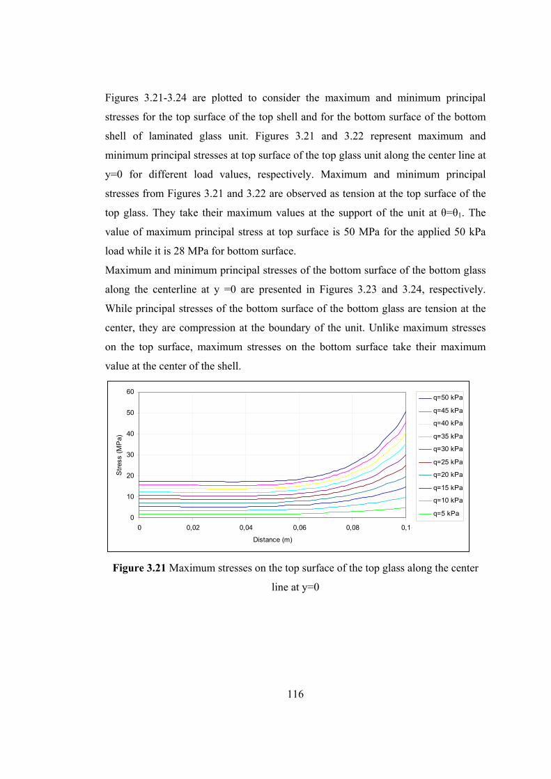
116
Figures 3.21-3.24 are plotted to consider the maximum and minimum principal
stresses for the top surface of the top shell and for the bottom surface of the bottom
shell of laminated glass unit. Figures 3.21 and 3.22 represent maximum and
minimum principal stresses at top surface of the top glass unit along the center line at
y=0 for different load values, respectively. Maximum and minimum principal
stresses from Figures 3.21 and 3.22 are observed as tension at the top surface of the
top glass. They take their maximum values at the support of the unit at θ=θ1. The
value of maximum principal stress at top surface is 50 MPa for the applied 50 kPa
load while it is 28 MPa for bottom surface.
Maximum and minimum principal stresses of the bottom surface of the bottom glass
along the centerline at y =0 are presented in Figures 3.23 and 3.24, respectively.
While principal stresses of the bottom surface of the bottom glass are tension at the
center, they are compression at the boundary of the unit. Unlike maximum stresses
on the top surface, maximum stresses on the bottom surface take their maximum
value at the center of the shell.
0
10
20
30
40
50
60
0 0,02 0,04 0,06 0,08 0,1
Distance (m)
Str
ess
(MP
a)
q=50 kPa
q=45 kPa
q=40 kPa
q=35 kPa
q=30 kPa
q=25 kPa
q=20 kPa
q=15 kPa
q=10 kPa
q=5 kPa
Figure 3.21 Maximum stresses on the top surface of the top glass along the center
line at y=0
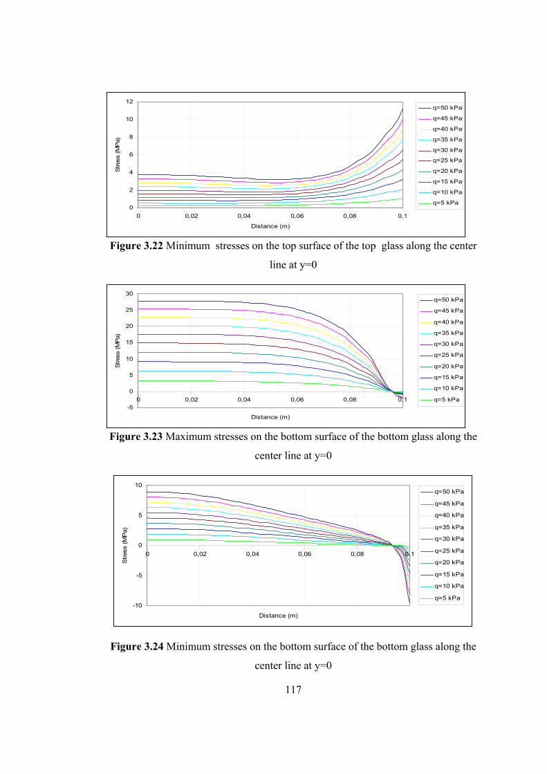
117
0
2
4
6
8
10
12
0 0,02 0,04 0,06 0,08 0,1
Distance (m)
Stres
s (M
Pa)
q=50 kPa
q=45 kPa
q=40 kPa
q=35 kPa
q=30 kPa
q=25 kPa
q=20 kPa
q=15 kPa
q=10 kPa
q=5 kPa
Figure 3.22 Minimum stresses on the top surface of the top glass along the center
line at y=0
-5
0
5
10
15
20
25
30
0 0,02 0,04 0,06 0,08 0,1
Distance (m)
Stres
s (M
Pa)
q=50 kPa
q=45 kPa
q=40 kPa
q=35 kPa
q=30 kPa
q=25 kPa
q=20 kPa
q=15 kPa
q=10 kPa
q=5 kPa
Figure 3.23 Maximum stresses on the bottom surface of the bottom glass along the
center line at y=0
-10
-5
0
5
10
0 0,02 0,04 0,06 0,08 0,1
Distance (m)
Stres
s (M
Pa)
q=50 kPa
q=45 kPa
q=40 kPa
q=35 kPa
q=30 kPa
q=25 kPa
q=20 kPa
q=15 kPa
q=10 kPa
q=5 kPa
Figure 3.24 Minimum stresses on the bottom surface of the bottom glass along the
center line at y=0
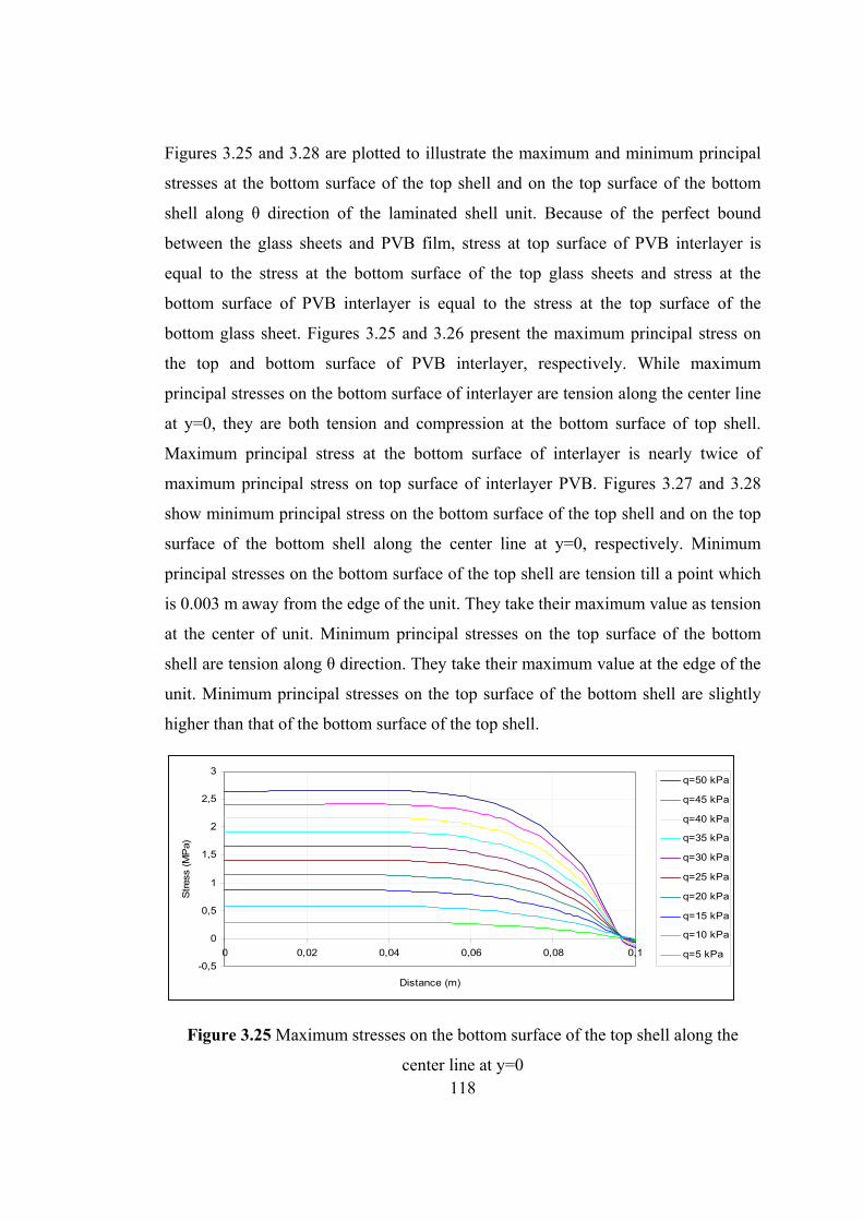
118
Figures 3.25 and 3.28 are plotted to illustrate the maximum and minimum principal
stresses at the bottom surface of the top shell and on the top surface of the bottom
shell along θ direction of the laminated shell unit. Because of the perfect bound
between the glass sheets and PVB film, stress at top surface of PVB interlayer is
equal to the stress at the bottom surface of the top glass sheets and stress at the
bottom surface of PVB interlayer is equal to the stress at the top surface of the
bottom glass sheet. Figures 3.25 and 3.26 present the maximum principal stress on
the top and bottom surface of PVB interlayer, respectively. While maximum
principal stresses on the bottom surface of interlayer are tension along the center line
at y=0, they are both tension and compression at the bottom surface of top shell.
Maximum principal stress at the bottom surface of interlayer is nearly twice of
maximum principal stress on top surface of interlayer PVB. Figures 3.27 and 3.28
show minimum principal stress on the bottom surface of the top shell and on the top
surface of the bottom shell along the center line at y=0, respectively. Minimum
principal stresses on the bottom surface of the top shell are tension till a point which
is 0.003 m away from the edge of the unit. They take their maximum value as tension
at the center of unit. Minimum principal stresses on the top surface of the bottom
shell are tension along θ direction. They take their maximum value at the edge of the
unit. Minimum principal stresses on the top surface of the bottom shell are slightly
higher than that of the bottom surface of the top shell.
-0,5
0
0,5
1
1,5
2
2,5
3
0 0,02 0,04 0,06 0,08 0,1
Distance (m)
Str
ess
(MP
a)
q=50 kPa
q=45 kPa
q=40 kPa
q=35 kPa
q=30 kPa
q=25 kPa
q=20 kPa
q=15 kPa
q=10 kPa
q=5 kPa
Figure 3.25 Maximum stresses on the bottom surface of the top shell along the
center line at y=0
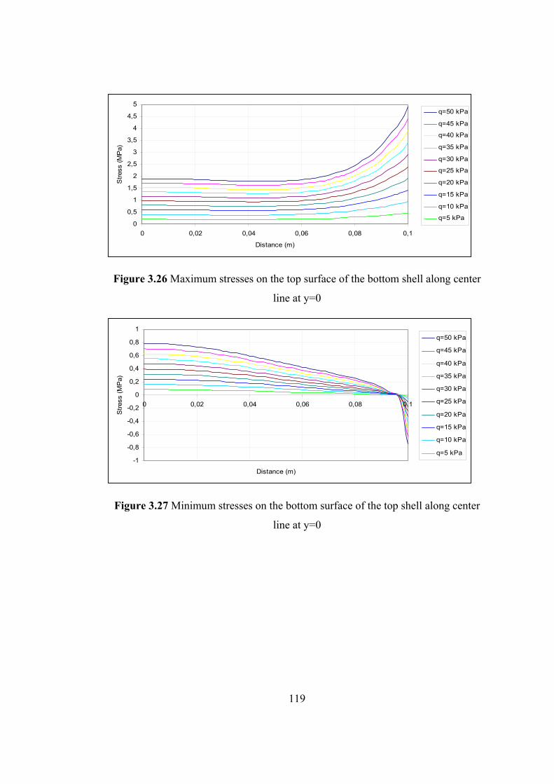
119
0
0,5
1
1,5
2
2,5
3
3,5
4
4,5
5
0 0,02 0,04 0,06 0,08 0,1
Distance (m)
Str
ess
(MP
a)q=50 kPa
q=45 kPa
q=40 kPa
q=35 kPa
q=30 kPa
q=25 kPa
q=20 kPa
q=15 kPa
q=10 kPa
q=5 kPa
Figure 3.26 Maximum stresses on the top surface of the bottom shell along center
line at y=0
-1
-0,8
-0,6
-0,4
-0,2
0
0,2
0,4
0,6
0,8
1
0 0,02 0,04 0,06 0,08 0,1
Distance (m)
Str
ess
(MP
a)
q=50 kPa
q=45 kPa
q=40 kPa
q=35 kPa
q=30 kPa
q=25 kPa
q=20 kPa
q=15 kPa
q=10 kPa
q=5 kPa
Figure 3.27 Minimum stresses on the bottom surface of the top shell along center
line at y=0
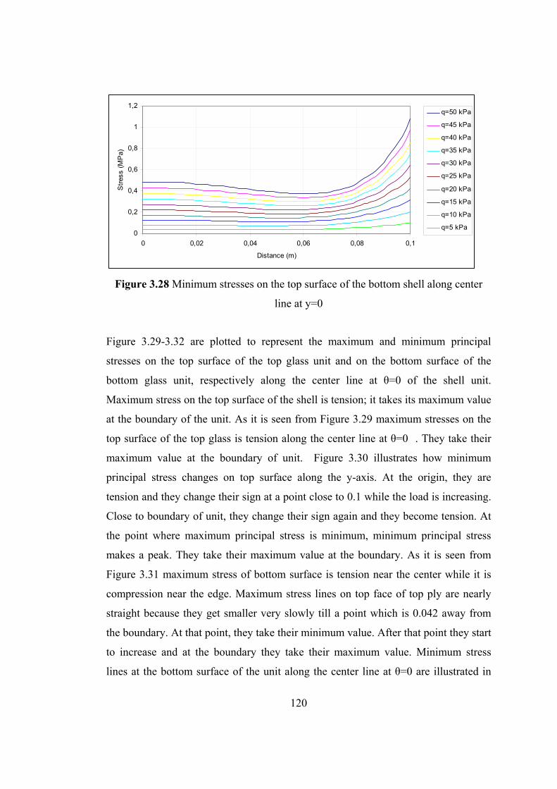
120
0
0,2
0,4
0,6
0,8
1
1,2
0 0,02 0,04 0,06 0,08 0,1
Distance (m)
Str
ess
(MP
a)q=50 kPa
q=45 kPa
q=40 kPa
q=35 kPa
q=30 kPa
q=25 kPa
q=20 kPa
q=15 kPa
q=10 kPa
q=5 kPa
Figure 3.28 Minimum stresses on the top surface of the bottom shell along center
line at y=0
Figure 3.29-3.32 are plotted to represent the maximum and minimum principal
stresses on the top surface of the top glass unit and on the bottom surface of the
bottom glass unit, respectively along the center line at θ=0 of the shell unit.
Maximum stress on the top surface of the shell is tension; it takes its maximum value
at the boundary of the unit. As it is seen from Figure 3.29 maximum stresses on the
top surface of the top glass is tension along the center line at θ=0 . They take their
maximum value at the boundary of unit. Figure 3.30 illustrates how minimum
principal stress changes on top surface along the y-axis. At the origin, they are
tension and they change their sign at a point close to 0.1 while the load is increasing.
Close to boundary of unit, they change their sign again and they become tension. At
the point where maximum principal stress is minimum, minimum principal stress
makes a peak. They take their maximum value at the boundary. As it is seen from
Figure 3.31 maximum stress of bottom surface is tension near the center while it is
compression near the edge. Maximum stress lines on top face of top ply are nearly
straight because they get smaller very slowly till a point which is 0.042 away from
the boundary. At that point, they take their minimum value. After that point they start
to increase and at the boundary they take their maximum value. Minimum stress
lines at the bottom surface of the unit along the center line at θ=0 are illustrated in
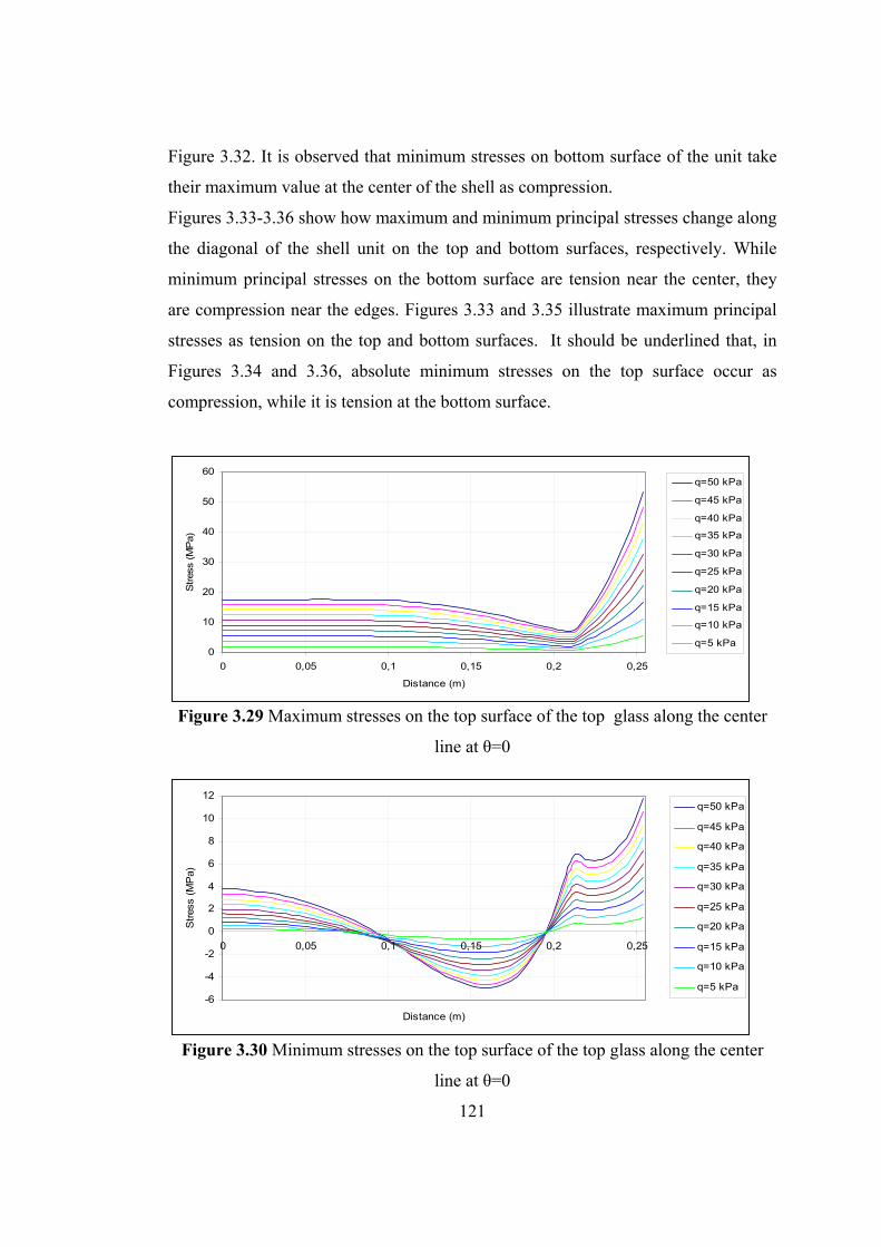
121
Figure 3.32. It is observed that minimum stresses on bottom surface of the unit take
their maximum value at the center of the shell as compression.
Figures 3.33-3.36 show how maximum and minimum principal stresses change along
the diagonal of the shell unit on the top and bottom surfaces, respectively. While
minimum principal stresses on the bottom surface are tension near the center, they
are compression near the edges. Figures 3.33 and 3.35 illustrate maximum principal
stresses as tension on the top and bottom surfaces. It should be underlined that, in
Figures 3.34 and 3.36, absolute minimum stresses on the top surface occur as
compression, while it is tension at the bottom surface.
0
10
20
30
40
50
60
0 0,05 0,1 0,15 0,2 0,25
Distance (m)
Stres
s (M
Pa)
q=50 kPa
q=45 kPa
q=40 kPa
q=35 kPa
q=30 kPa
q=25 kPa
q=20 kPa
q=15 kPa
q=10 kPa
q=5 kPa
Figure 3.29 Maximum stresses on the top surface of the top glass along the center
line at θ=0
-6
-4
-2
0
2
4
6
8
10
12
0 0,05 0,1 0,15 0,2 0,25
Distance (m)
Str
ess
(MP
a)
q=50 kPa
q=45 kPa
q=40 kPa
q=35 kPa
q=30 kPa
q=25 kPa
q=20 kPa
q=15 kPa
q=10 kPa
q=5 kPa
Figure 3.30 Minimum stresses on the top surface of the top glass along the center
line at θ=0
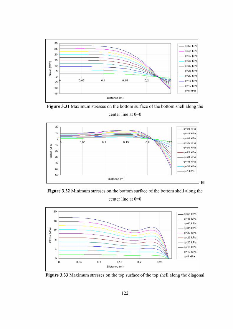
122
-15
-10
-5
0
5
10
15
20
25
30
0 0,05 0,1 0,15 0,2 0,25
Distance (m)
Stres
s (M
Pa)
q=50 kPa
q=45 kPa
q=40 kPa
q=35 kPa
q=30 kPa
q=25 kPa
q=20 kPa
q=15 kPa
q=10 kPa
q=5 kPa
Figure 3.31 Maximum stresses on the bottom surface of the bottom shell along the
center line at θ=0
-60
-50
-40
-30
-20
-10
0
10
20
0 0,05 0,1 0,15 0,2 0,25
Distance (m)
Stres
s (M
Pa)
q=50 kPa
q=45 kPa
q=40 kPa
q=35 kPa
q=30 kPa
q=25 kPa
q=20 kPa
q=15 kPa
q=10 kPa
q=5 kPa
Fi
Figure 3.32 Minimum stresses on the bottom surface of the bottom shell along the
center line at θ=0
0
4
8
12
16
20
0 0,05 0,1 0,15 0,2 0,25
Distance (m)
Stres
s (M
Pa)
q=50 kPa
q=45 kPa
q=40 kPa
q=35 kPa
q=30 kPa
q=25 kPa
q=20 kPa
q=15 kPa
q=10 kPa
q=5 kPa
Figure 3.33 Maximum stresses on the top surface of the top shell along the diagonal
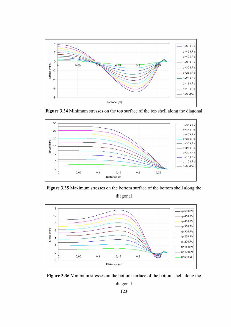
123
-8
-6
-4
-2
0
2
4
0 0,05 0,1 0,15 0,2 0,25
Distance (m)
Str
ess
(MP
a)q=50 kPa
q=45 kPa
q=40 kPa
q=35 kPa
q=30 kPa
q=25 kPa
q=20 kPa
q=15 kPa
q=10 kPa
q=5 kPa
Figure 3.34 Minimum stresses on the top surface of the top shell along the diagonal
0
5
10
15
20
25
30
0 0,05 0,1 0,15 0,2 0,25
Distance (m)
Stres
s (M
Pa)
q=50 kPa
q=45 kPa
q=40 kPa
q=35 kPa
q=30 kPa
q=25 kPa
q=20 kPa
q=15 kPa
q=10 kPa
q=5 kPa
Figure 3.35 Maximum stresses on the bottom surface of the bottom shell along the
diagonal
-2
0
2
4
6
8
10
12
0 0,05 0,1 0,15 0,2 0,25
Distance (m)
Stres
s (M
Pa)
q=50 kPa
q=45 kPa
q=40 kPa
q=35 kPa
q=30 kPa
q=25 kPa
q=20 kPa
q=15 kPa
q=10 kPa
q=5 kPa
Figure 3.36 Minimum stresses on the bottom surface of the bottom shell along the
diagonal
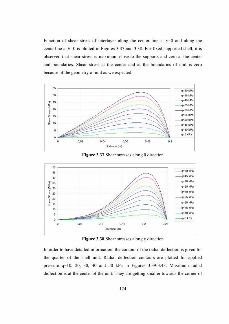
124
Function of shear stress of interlayer along the center line at y=0 and along the
centerline at θ=0 is plotted in Figures 3.37 and 3.38. For fixed supported shell, it is
observed that shear stress is maximum close to the supports and zero at the center
and boundaries. Shear stress at the center and at the boundaries of unit is zero
because of the geometry of unit as we expected.
0
5
10
15
20
25
30
35
0 0,02 0,04 0,06 0,08 0,1
Distance (m)
She
ar S
tres
s (M
Pa)
q=50 kPa
q=45 kPa
q=40 kPa
q=35 kPa
q=30 kPa
q=25 kPa
q=20 kPa
q=15 kPa
q=10 kPa
q=5 kPa
Figure 3.37 Shear stresses along θ direction
0
5
10
15
20
25
30
35
40
45
50
0 0,05 0,1 0,15 0,2 0,25
Distance (m)
She
ar S
tres
s (M
Pa)
q=50 kPa
q=45 kPa
q=40 kPa
q=35 kPa
q=30 kPa
q=25 kPa
q=20 kPa
q=15 kPa
q=10 kPa
q=5 kPa
Figure 3.38 Shear stresses along y direction
In order to have detailed information, the contour of the radial deflection is given for
the quarter of the shell unit. Radial deflection contours are plotted for applied
pressure q=10, 20, 30, 40 and 50 kPa in Figures 3.39-3.43. Maximum radial
deflection is at the center of the unit. They are getting smaller towards the corner of
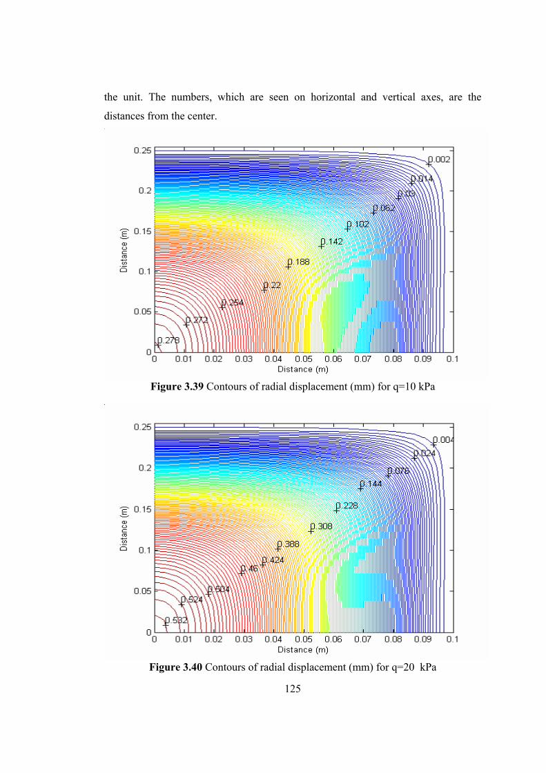
125
the unit. The numbers, which are seen on horizontal and vertical axes, are the
distances from the center.
Figure 3.39 Contours of radial displacement (mm) for q=10 kPa
Figure 3.40 Contours of radial displacement (mm) for q=20 kPa
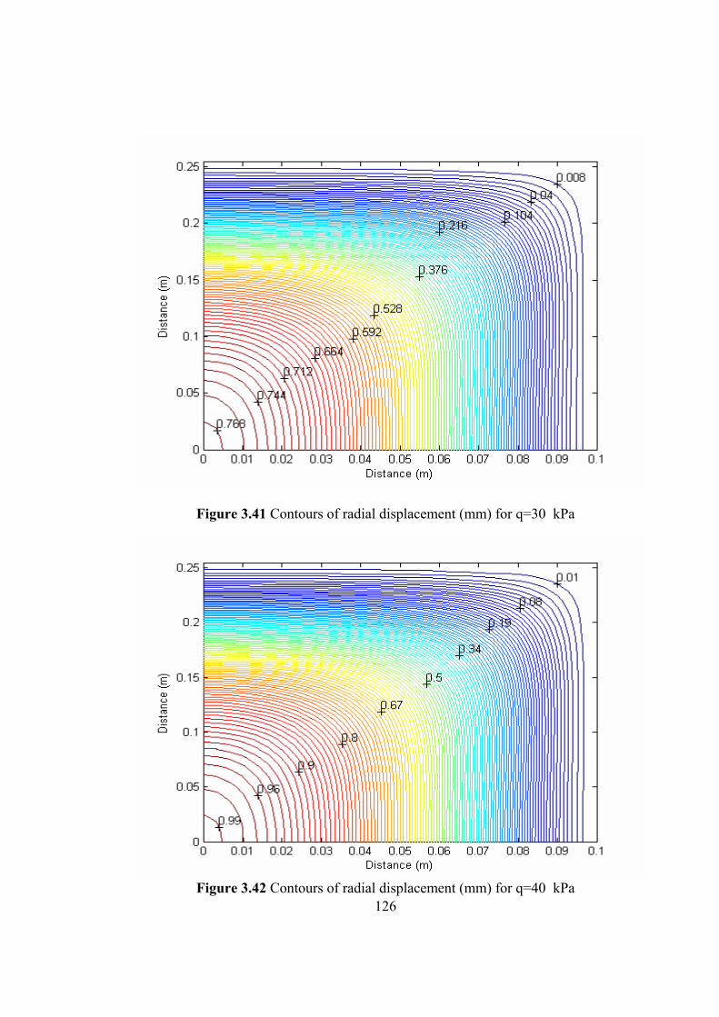
126
Figure 3.41 Contours of radial displacement (mm) for q=30 kPa
Figure 3.42 Contours of radial displacement (mm) for q=40 kPa
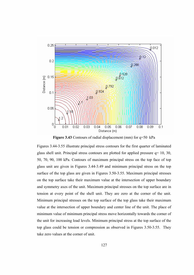
127
Figure 3.43 Contours of radial displacement (mm) for q=50 kPa
Figures 3.44-3.55 illustrate principal stress contours for the first quarter of laminated
glass shell unit. Principal stress contours are plotted for applied pressure q= 10, 30,
50, 70, 90, 100 kPa. Contours of maximum principal stress on the top face of top
glass unit are given in Figures 3.44-3.49 and minimum principal stress on the top
surface of the top glass are given in Figures 3.50-3.55. Maximum principal stresses
on the top surface take their maximum value at the intersection of upper boundary
and symmetry axes of the unit. Maximum principal stresses on the top surface are in
tension at every point of the shell unit. They are zero at the corner of the unit.
Minimum principal stresses on the top surface of the top glass take their maximum
value at the intersection of upper boundary and center line of the unit. The place of
minimum value of minimum principal stress move horizontally towards the corner of
the unit for increasing load levels. Minimum principal stress at the top surface of the
top glass could be tension or compression as observed in Figures 3.50-3.55. They
take zero values at the corner of unit.
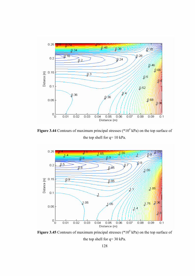
128
Figure 3.44 Contours of maximum principal stresses (*104 kPa) on the top surface of
the top shell for q= 10 kPa.
Figure 3.45 Contours of maximum principal stresses (*104 kPa) on the top surface of
the top shell for q= 30 kPa.
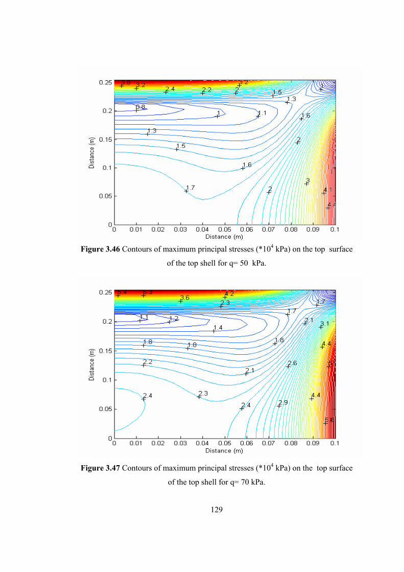
129
Figure 3.46 Contours of maximum principal stresses (*104 kPa) on the top surface
of the top shell for q= 50 kPa.
Figure 3.47 Contours of maximum principal stresses (*104 kPa) on the top surface
of the top shell for q= 70 kPa.
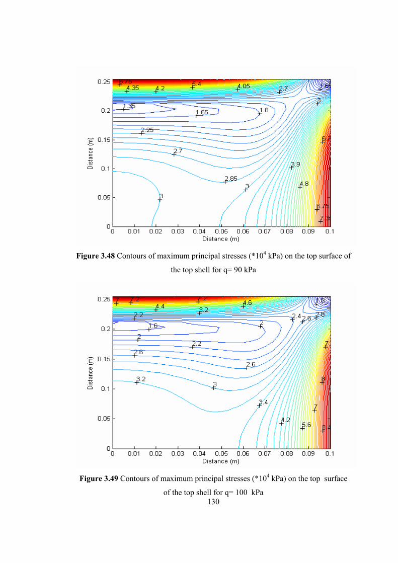
130
Figure 3.48 Contours of maximum principal stresses (*104 kPa) on the top surface of
the top shell for q= 90 kPa
Figure 3.49 Contours of maximum principal stresses (*104 kPa) on the top surface
of the top shell for q= 100 kPa
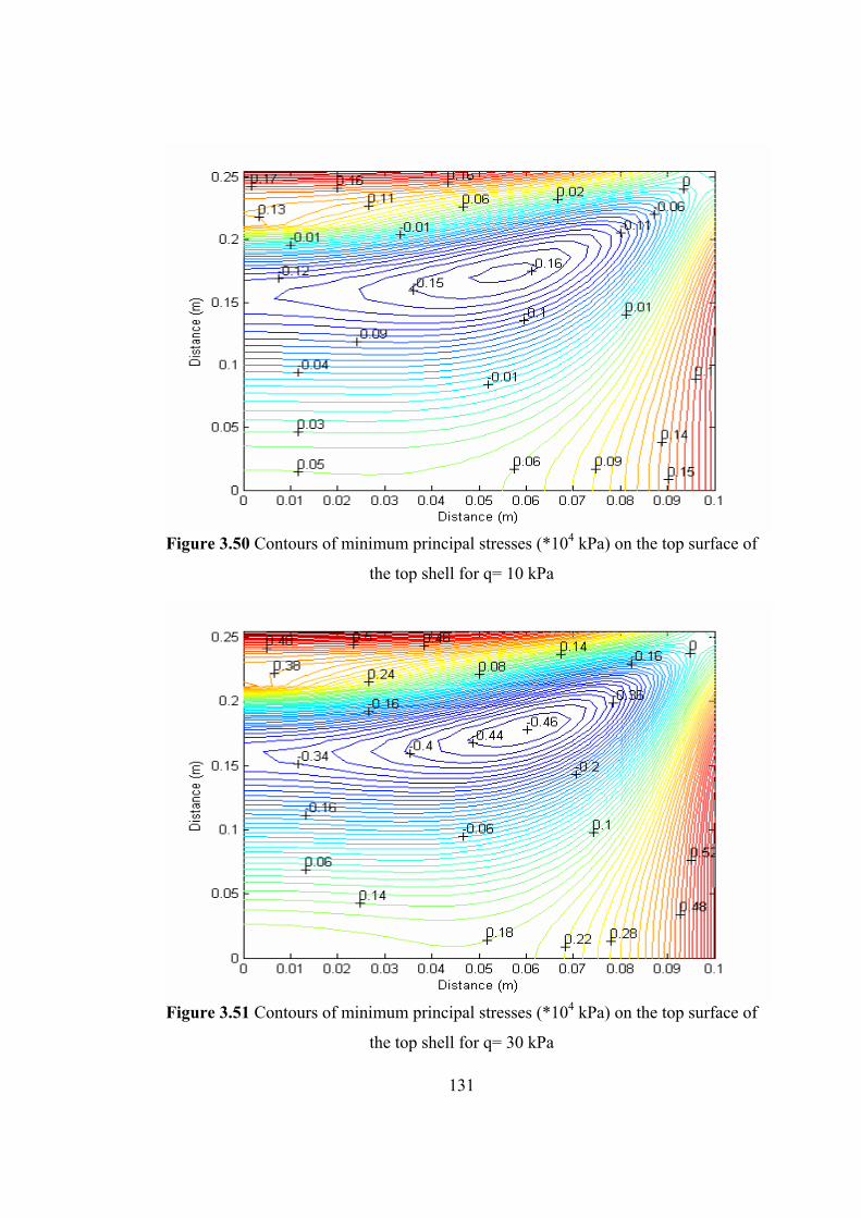
131
Figure 3.50 Contours of minimum principal stresses (*104 kPa) on the top surface of
the top shell for q= 10 kPa
Figure 3.51 Contours of minimum principal stresses (*104 kPa) on the top surface of
the top shell for q= 30 kPa
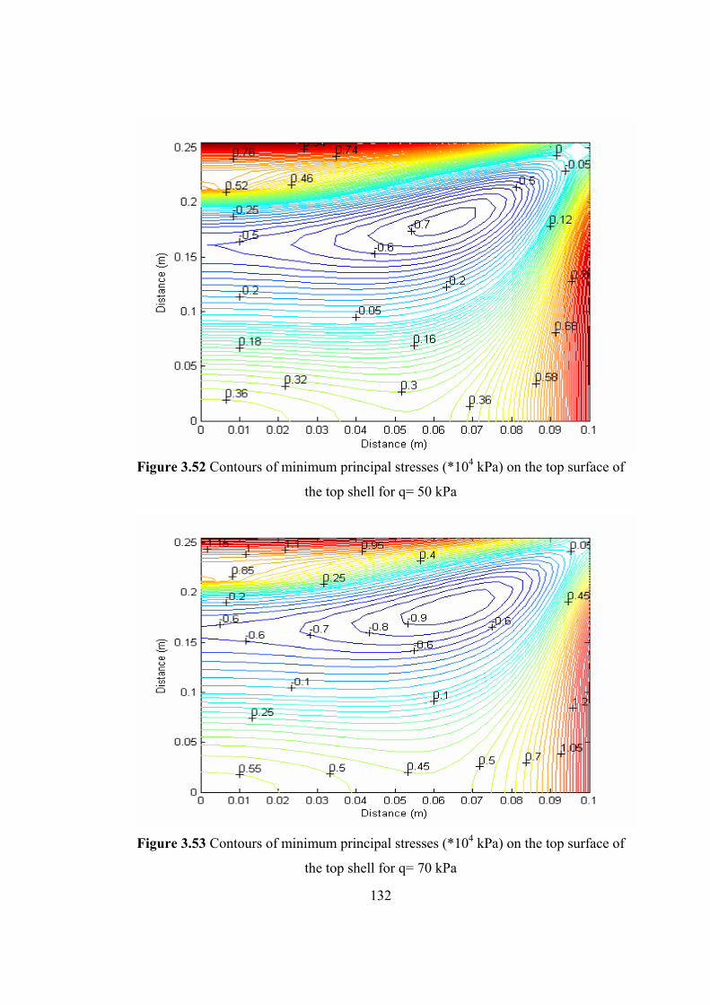
132
Figure 3.52 Contours of minimum principal stresses (*104 kPa) on the top surface of
the top shell for q= 50 kPa
Figure 3.53 Contours of minimum principal stresses (*104 kPa) on the top surface of
the top shell for q= 70 kPa
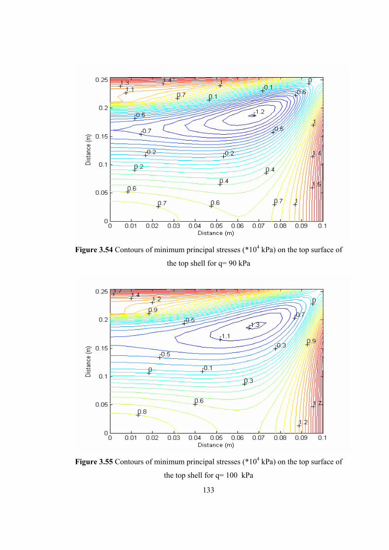
133
Figure 3.54 Contours of minimum principal stresses (*104 kPa) on the top surface of
the top shell for q= 90 kPa
Figure 3.55 Contours of minimum principal stresses (*104 kPa) on the top surface of
the top shell for q= 100 kPa
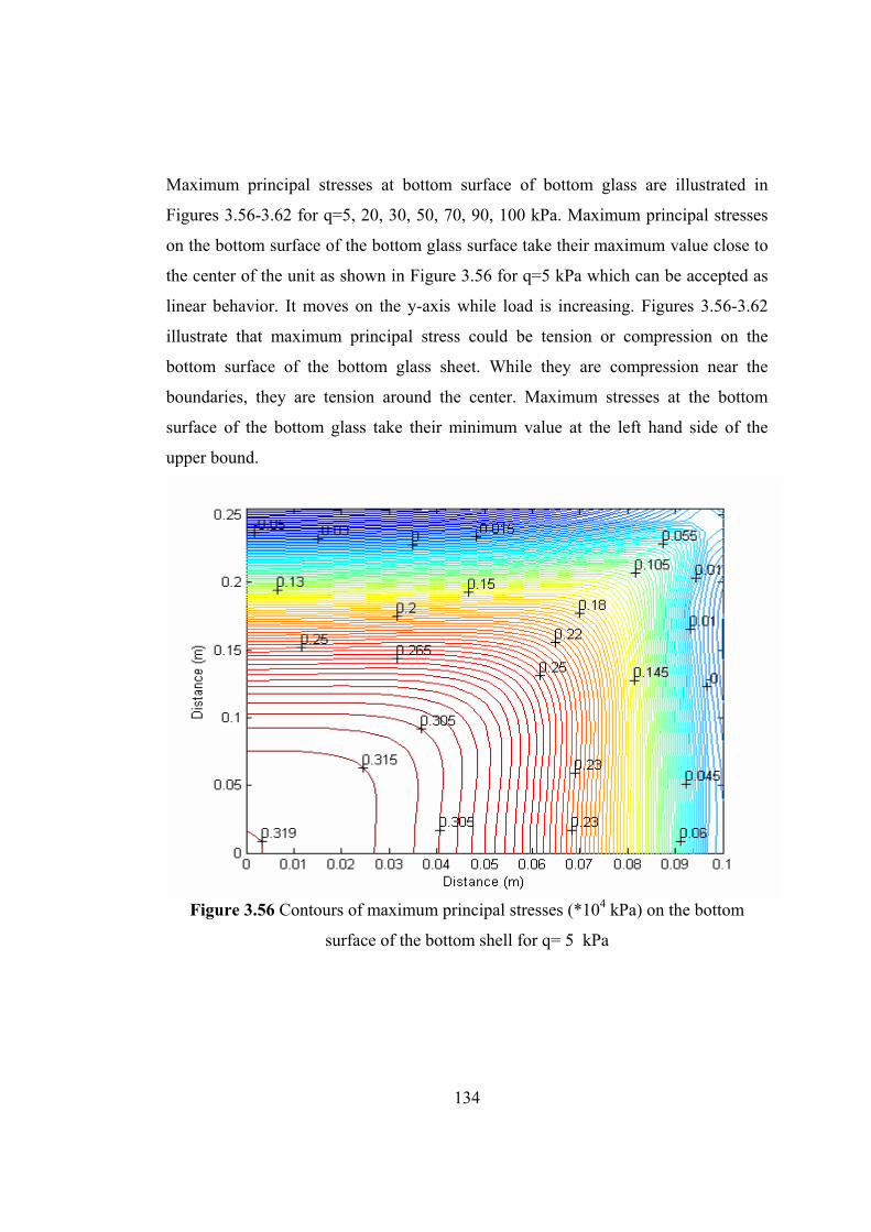
134
Maximum principal stresses at bottom surface of bottom glass are illustrated in
Figures 3.56-3.62 for q=5, 20, 30, 50, 70, 90, 100 kPa. Maximum principal stresses
on the bottom surface of the bottom glass surface take their maximum value close to
the center of the unit as shown in Figure 3.56 for q=5 kPa which can be accepted as
linear behavior. It moves on the y-axis while load is increasing. Figures 3.56-3.62
illustrate that maximum principal stress could be tension or compression on the
bottom surface of the bottom glass sheet. While they are compression near the
boundaries, they are tension around the center. Maximum stresses at the bottom
surface of the bottom glass take their minimum value at the left hand side of the
upper bound.
Figure 3.56 Contours of maximum principal stresses (*104 kPa) on the bottom
surface of the bottom shell for q= 5 kPa
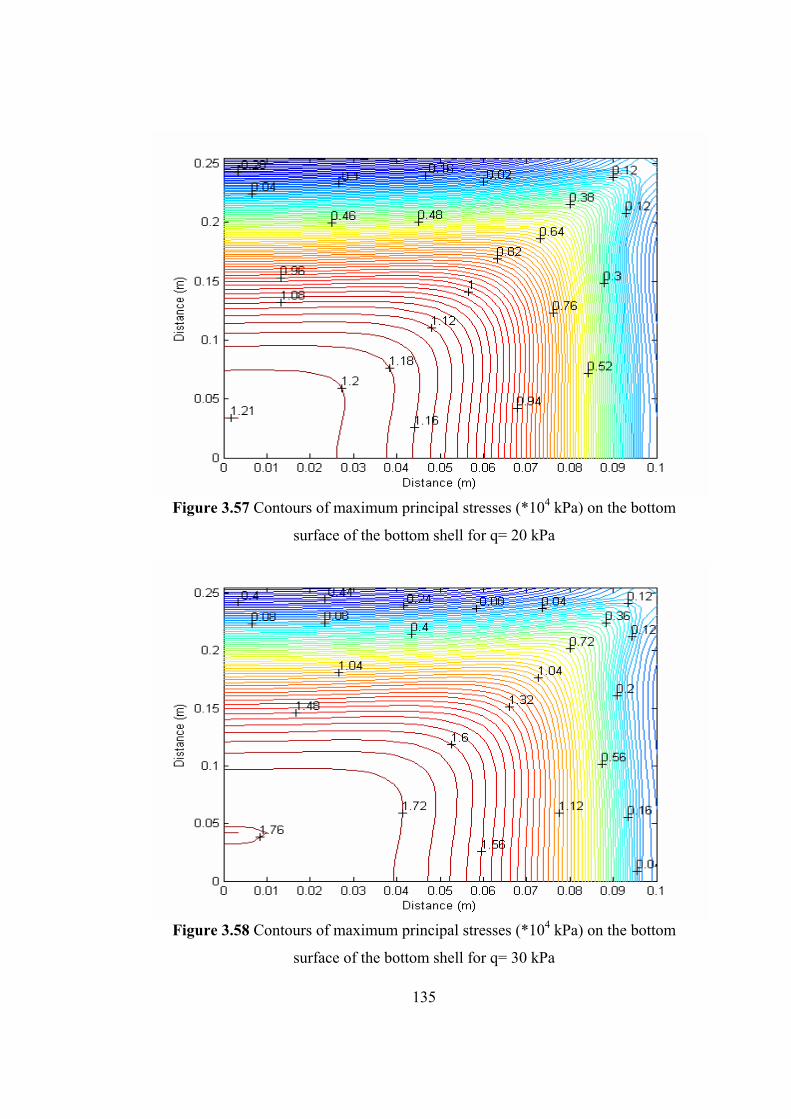
135
Figure 3.57 Contours of maximum principal stresses (*104 kPa) on the bottom
surface of the bottom shell for q= 20 kPa
Figure 3.58 Contours of maximum principal stresses (*104 kPa) on the bottom
surface of the bottom shell for q= 30 kPa
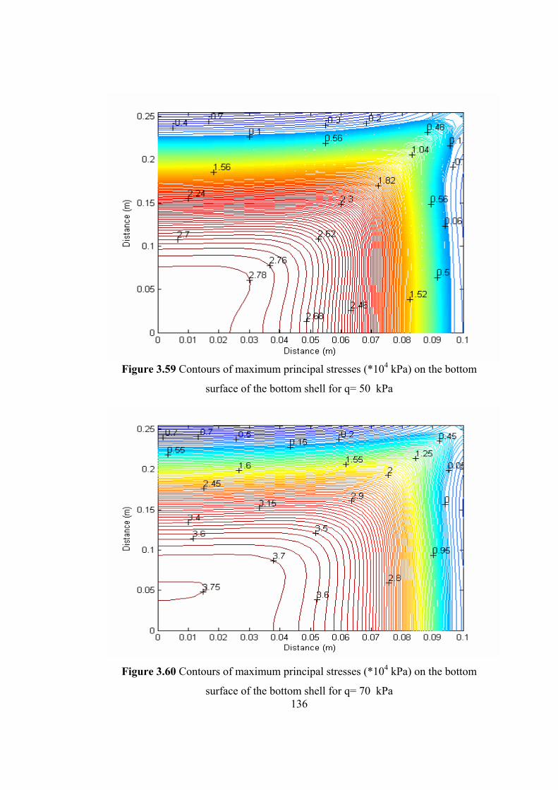
136
Figure 3.59 Contours of maximum principal stresses (*104 kPa) on the bottom
surface of the bottom shell for q= 50 kPa
Figure 3.60 Contours of maximum principal stresses (*104 kPa) on the bottom
surface of the bottom shell for q= 70 kPa
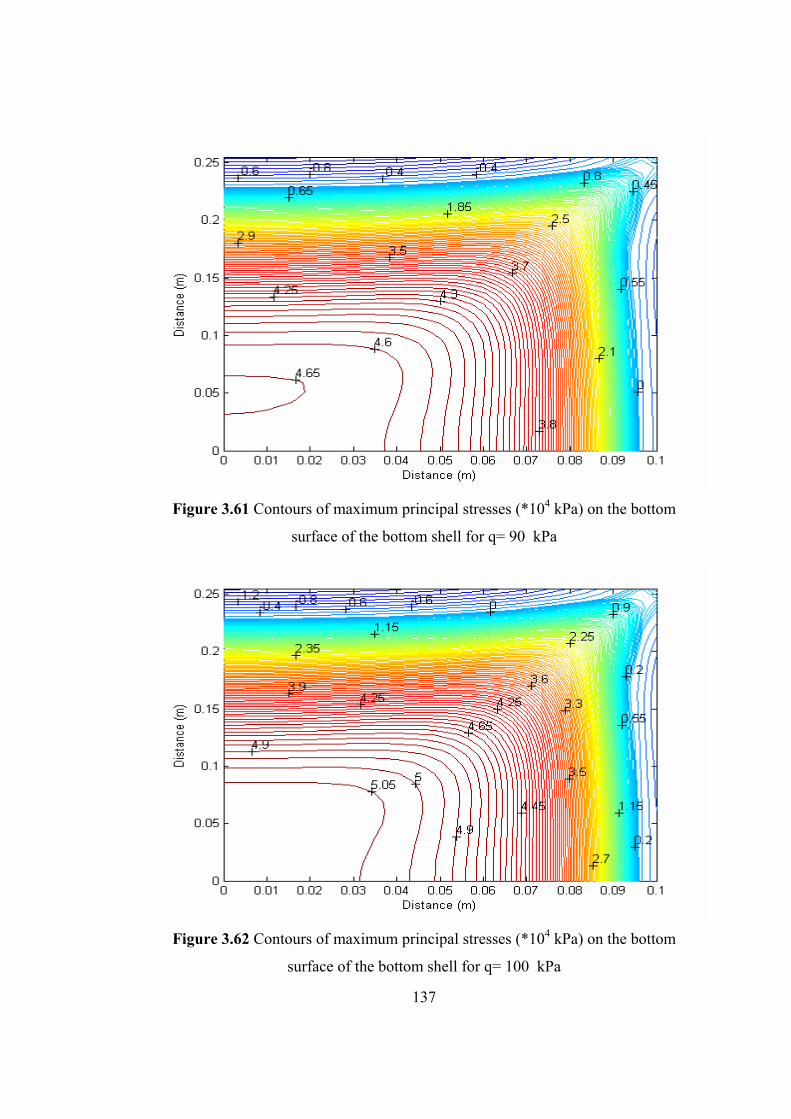
137
Figure 3.61 Contours of maximum principal stresses (*104 kPa) on the bottom
surface of the bottom shell for q= 90 kPa
Figure 3.62 Contours of maximum principal stresses (*104 kPa) on the bottom
surface of the bottom shell for q= 100 kPa
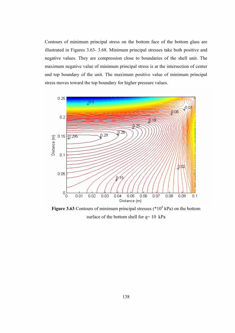
138
Contours of minimum principal stress on the bottom face of the bottom glass are
illustrated in Figures 3.63- 3.68. Minimum principal stresses take both positive and
negative values. They are compression close to boundaries of the shell unit. The
maximum negative value of minimum principal stress is at the intersection of center
and top boundary of the unit. The maximum positive value of minimum principal
stress moves toward the top boundary for higher pressure values.
Figure 3.63 Contours of minimum principal stresses (*104 kPa) on the bottom
surface of the bottom shell for q= 10 kPa
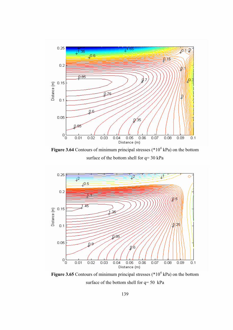
139
Figure 3.64 Contours of minimum principal stresses (*104 kPa) on the bottom
surface of the bottom shell for q= 30 kPa
Figure 3.65 Contours of minimum principal stresses (*104 kPa) on the bottom
surface of the bottom shell for q= 50 kPa
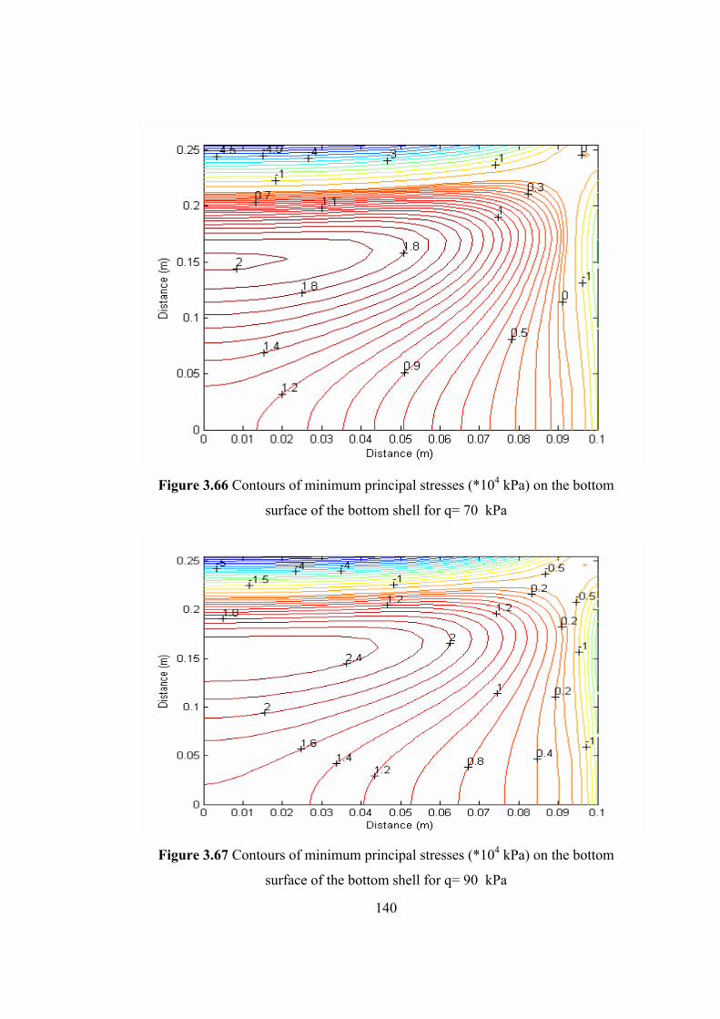
140
Figure 3.66 Contours of minimum principal stresses (*104 kPa) on the bottom
surface of the bottom shell for q= 70 kPa
Figure 3.67 Contours of minimum principal stresses (*104 kPa) on the bottom
surface of the bottom shell for q= 90 kPa
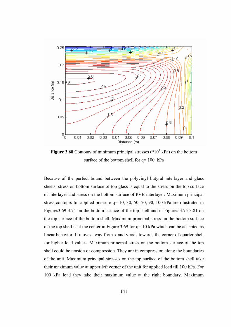
141
Figure 3.68 Contours of minimum principal stresses (*104 kPa) on the bottom
surface of the bottom shell for q= 100 kPa
Because of the perfect bound between the polyvinyl butyral interlayer and glass
sheets, stress on bottom surface of top glass is equal to the stress on the top surface
of interlayer and stress on the bottom surface of PVB interlayer. Maximum principal
stress contours for applied pressure q= 10, 30, 50, 70, 90, 100 kPa are illustrated in
Figures3.69-3.74 on the bottom surface of the top shell and in Figures 3.75-3.81 on
the top surface of the bottom shell. Maximum principal stress on the bottom surface
of the top shell is at the center in Figure 3.69 for q= 10 kPa which can be accepted as
linear behavior. It moves away from x and y-axis towards the corner of quarter shell
for higher load values. Maximum principal stress on the bottom surface of the top
shell could be tension or compression. They are in compression along the boundaries
of the unit. Maximum principal stresses on the top surface of the bottom shell take
their maximum value at upper left corner of the unit for applied load till 100 kPa. For
100 kPa load they take their maximum value at the right boundary. Maximum
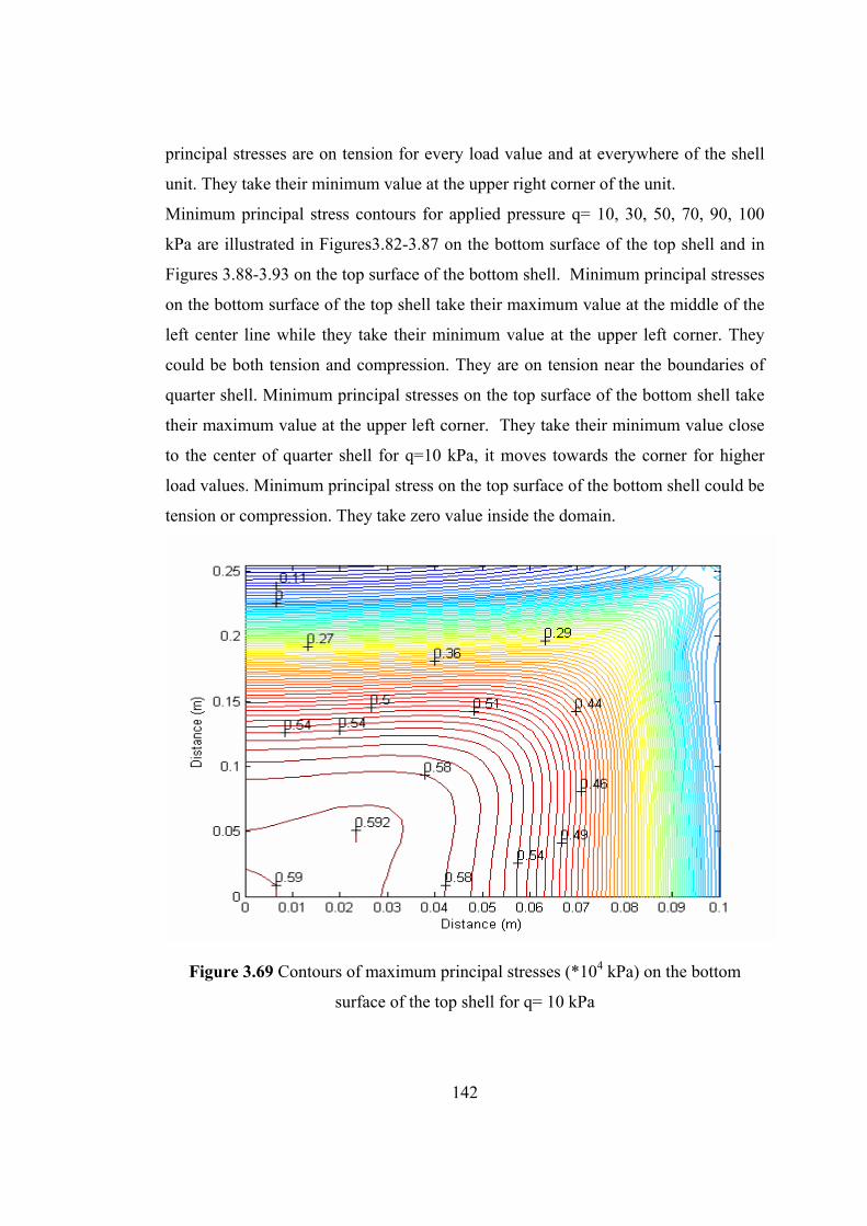
142
principal stresses are on tension for every load value and at everywhere of the shell
unit. They take their minimum value at the upper right corner of the unit.
Minimum principal stress contours for applied pressure q= 10, 30, 50, 70, 90, 100
kPa are illustrated in Figures3.82-3.87 on the bottom surface of the top shell and in
Figures 3.88-3.93 on the top surface of the bottom shell. Minimum principal stresses
on the bottom surface of the top shell take their maximum value at the middle of the
left center line while they take their minimum value at the upper left corner. They
could be both tension and compression. They are on tension near the boundaries of
quarter shell. Minimum principal stresses on the top surface of the bottom shell take
their maximum value at the upper left corner. They take their minimum value close
to the center of quarter shell for q=10 kPa, it moves towards the corner for higher
load values. Minimum principal stress on the top surface of the bottom shell could be
tension or compression. They take zero value inside the domain.
Figure 3.69 Contours of maximum principal stresses (*104 kPa) on the bottom
surface of the top shell for q= 10 kPa
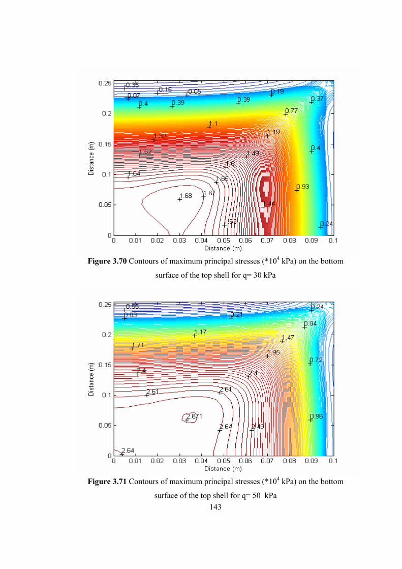
143
Figure 3.70 Contours of maximum principal stresses (*104 kPa) on the bottom
surface of the top shell for q= 30 kPa
Figure 3.71 Contours of maximum principal stresses (*104 kPa) on the bottom
surface of the top shell for q= 50 kPa
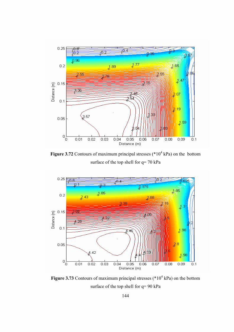
144
Figure 3.72 Contours of maximum principal stresses (*104 kPa) on the bottom
surface of the top shell for q= 70 kPa
Figure 3.73 Contours of maximum principal stresses (*104 kPa) on the bottom
surface of the top shell for q= 90 kPa
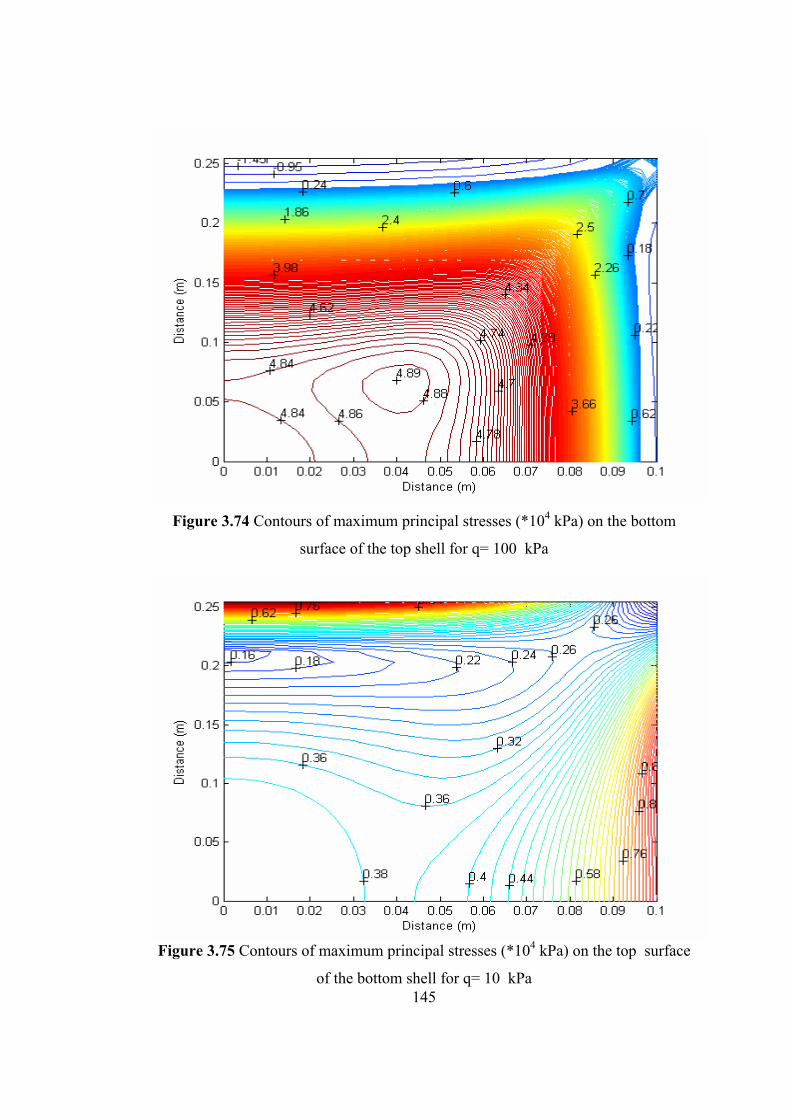
145
Figure 3.74 Contours of maximum principal stresses (*104 kPa) on the bottom
surface of the top shell for q= 100 kPa
Figure 3.75 Contours of maximum principal stresses (*104 kPa) on the top surface
of the bottom shell for q= 10 kPa
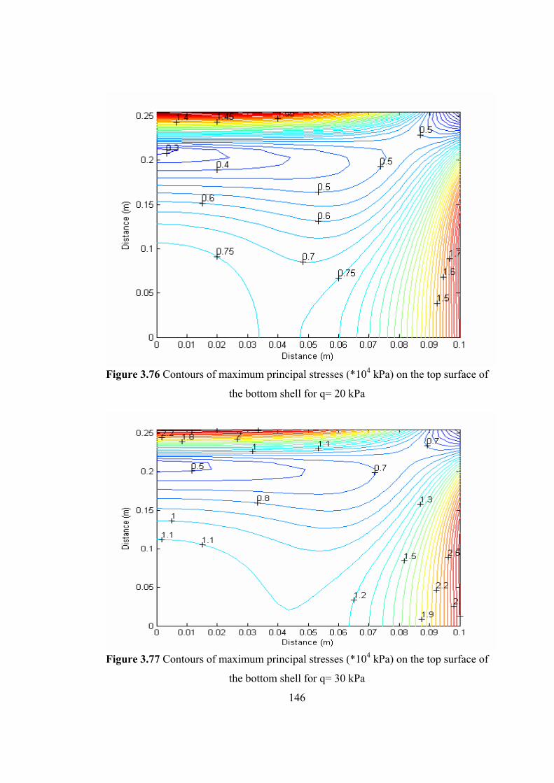
146
Figure 3.76 Contours of maximum principal stresses (*104 kPa) on the top surface of
the bottom shell for q= 20 kPa
Figure 3.77 Contours of maximum principal stresses (*104 kPa) on the top surface of
the bottom shell for q= 30 kPa
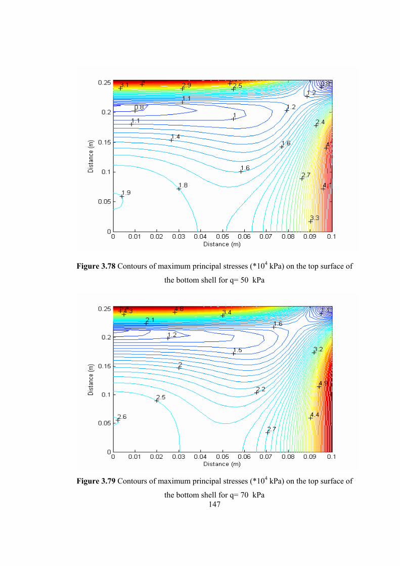
147
Figure 3.78 Contours of maximum principal stresses (*104 kPa) on the top surface of
the bottom shell for q= 50 kPa
Figure 3.79 Contours of maximum principal stresses (*104 kPa) on the top surface of
the bottom shell for q= 70 kPa
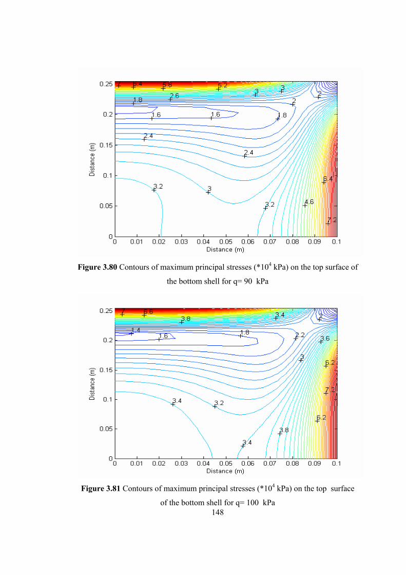
148
Figure 3.80 Contours of maximum principal stresses (*104 kPa) on the top surface of
the bottom shell for q= 90 kPa
Figure 3.81 Contours of maximum principal stresses (*104 kPa) on the top surface
of the bottom shell for q= 100 kPa
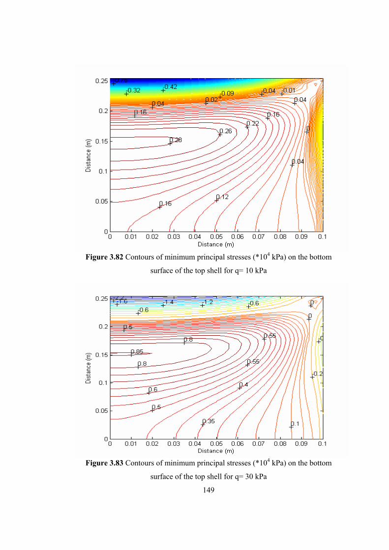
149
Figure 3.82 Contours of minimum principal stresses (*104 kPa) on the bottom
surface of the top shell for q= 10 kPa
Figure 3.83 Contours of minimum principal stresses (*104 kPa) on the bottom
surface of the top shell for q= 30 kPa
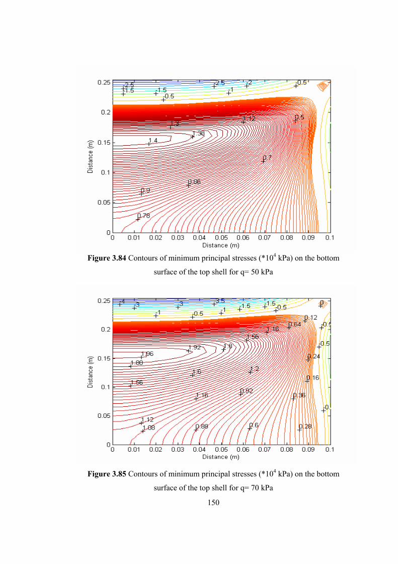
150
Figure 3.84 Contours of minimum principal stresses (*104 kPa) on the bottom
surface of the top shell for q= 50 kPa
Figure 3.85 Contours of minimum principal stresses (*104 kPa) on the bottom
surface of the top shell for q= 70 kPa
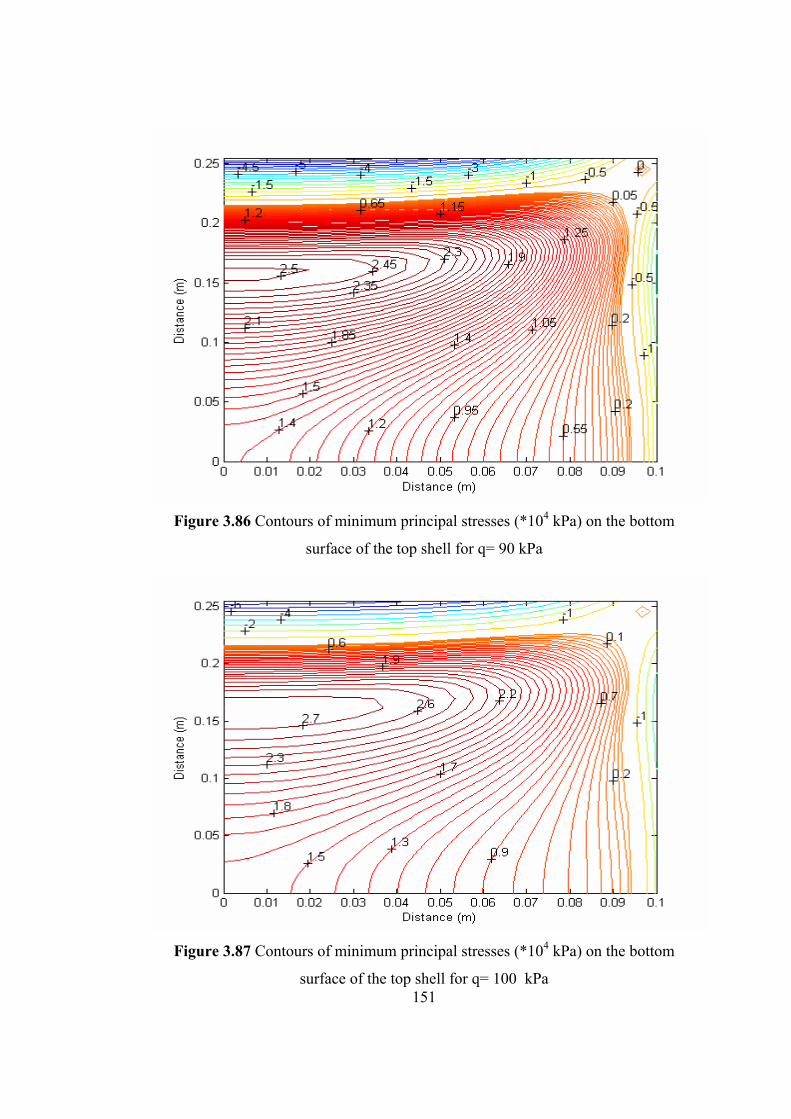
151
Figure 3.86 Contours of minimum principal stresses (*104 kPa) on the bottom
surface of the top shell for q= 90 kPa
Figure 3.87 Contours of minimum principal stresses (*104 kPa) on the bottom
surface of the top shell for q= 100 kPa
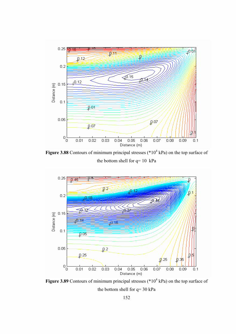
152
Figure 3.88 Contours of minimum principal stresses (*104 kPa) on the top surface of
the bottom shell for q= 10 kPa
Figure 3.89 Contours of minimum principal stresses (*104 kPa) on the top surface of
the bottom shell for q= 30 kPa
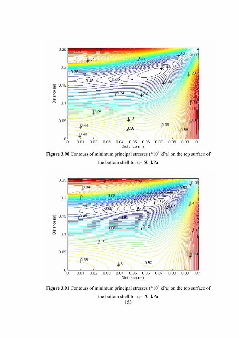
153
Figure 3.90 Contours of minimum principal stresses (*104 kPa) on the top surface of
the bottom shell for q= 50 kPa
Figure 3.91 Contours of minimum principal stresses (*104 kPa) on the top surface of
the bottom shell for q= 70 kPa
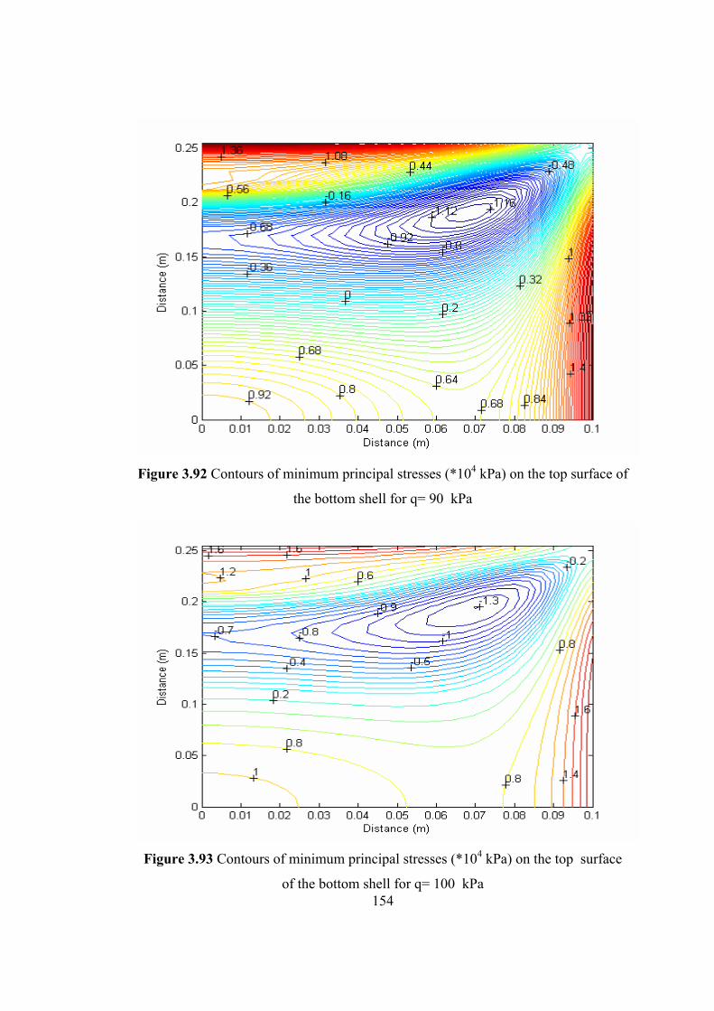
154
Figure 3.92 Contours of minimum principal stresses (*104 kPa) on the top surface of
the bottom shell for q= 90 kPa
Figure 3.93 Contours of minimum principal stresses (*104 kPa) on the top surface
of the bottom shell for q= 100 kPa
155
3.6.2 Strength Factor Analysis of Laminated Glass Unit
Theoretical stress analyses of monolithic and laminated glass units are conducted in
order to establish the limits of behavior of laminated glass units. The strength factor
(type factor) is defined as the ratio of maximum principal stress in monolithic glass
unit to the maximum principal stress in laminated glass unit. If the PVB interlayer is
strong enough to transfer 100 percent of shear between the glass sheets, then strength
factor 1.0 will mean that radial pressure resistance of monolithic and laminated glass
units are similar. Displacements and stress of laminated and monolithic glass units
are compared as in order to access the strength factor value of laminated glass unit.
The strength factor value for laminated unit is computed by using the formula below.
Unit Glass Laminated in StressPrincipal Maximum
Unit Glass c Monolithiin StressPrincipal MaximumFactor Strength
Because of large deformations in addition to the bending stresses, membrane stresses
occur while the radial pressures are increasing and this causes variation to the
strength factor.
For monolithic and laminated glass units, which have the same nominal glass
thickness, strength factor values are assigned in Table 3.4 below:
Table 3.4 Strength Factor values in building codes
Code Strength Factor Uniform Building Code 1985
Basic/National Building Code 1984 0.6
Standart Building Code 1986 Uniform Building Code 1988 Basic/National Building Code 1987
Standart Building Code 1988
0.75
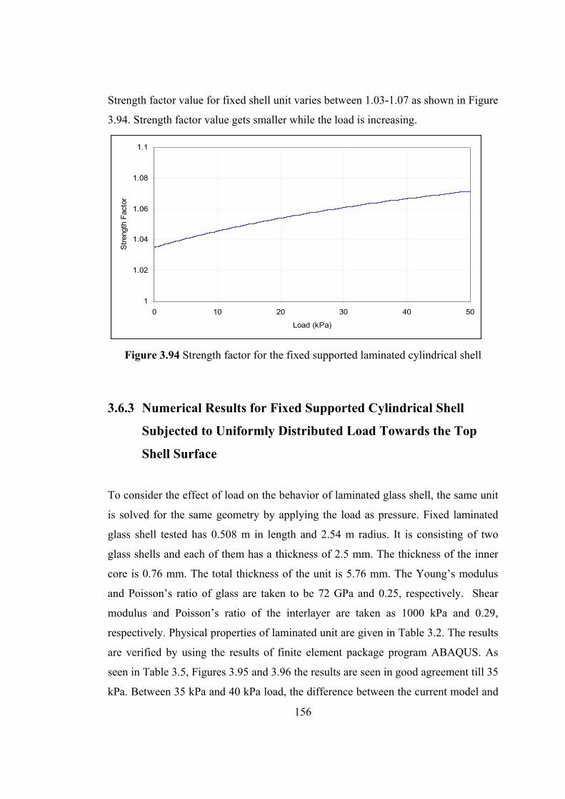
156
Strength factor value for fixed shell unit varies between 1.03-1.07 as shown in Figure
3.94. Strength factor value gets smaller while the load is increasing.
1
1.02
1.04
1.06
1.08
1.1
0 10 20 30 40 50
Load (kPa)
Str
engt
h F
acto
r
Figure 3.94 Strength factor for the fixed supported laminated cylindrical shell
3.6.3 Numerical Results for Fixed Supported Cylindrical Shell
Subjected to Uniformly Distributed Load Towards the Top
Shell Surface
To consider the effect of load on the behavior of laminated glass shell, the same unit
is solved for the same geometry by applying the load as pressure. Fixed laminated
glass shell tested has 0.508 m in length and 2.54 m radius. It is consisting of two
glass shells and each of them has a thickness of 2.5 mm. The thickness of the inner
core is 0.76 mm. The total thickness of the unit is 5.76 mm. The Young’s modulus
and Poisson’s ratio of glass are taken to be 72 GPa and 0.25, respectively. Shear
modulus and Poisson’s ratio of the interlayer are taken as 1000 kPa and 0.29,
respectively. Physical properties of laminated unit are given in Table 3.2. The results
are verified by using the results of finite element package program ABAQUS. As
seen in Table 3.5, Figures 3.95 and 3.96 the results are seen in good agreement till 35
kPa. Between 35 kPa and 40 kPa load, the difference between the current model and
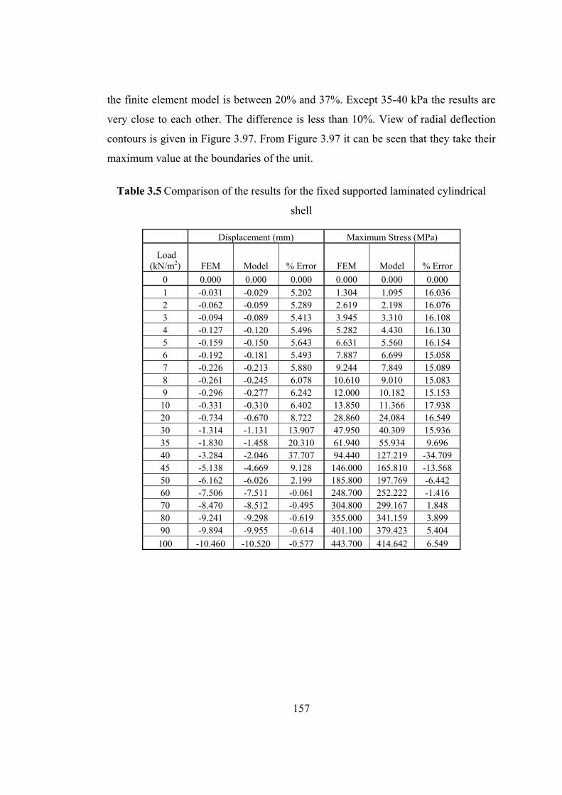
157
the finite element model is between 20% and 37%. Except 35-40 kPa the results are
very close to each other. The difference is less than 10%. View of radial deflection
contours is given in Figure 3.97. From Figure 3.97 it can be seen that they take their
maximum value at the boundaries of the unit.
Table 3.5 Comparison of the results for the fixed supported laminated cylindrical
shell
Displacement (mm) Maximum Stress (MPa)
Load (kN/m2) FEM Model % Error FEM Model % Error
0 0.000 0.000 0.000 0.000 0.000 0.000 1 -0.031 -0.029 5.202 1.304 1.095 16.036 2 -0.062 -0.059 5.289 2.619 2.198 16.076 3 -0.094 -0.089 5.413 3.945 3.310 16.108 4 -0.127 -0.120 5.496 5.282 4.430 16.130 5 -0.159 -0.150 5.643 6.631 5.560 16.154 6 -0.192 -0.181 5.493 7.887 6.699 15.058 7 -0.226 -0.213 5.880 9.244 7.849 15.089 8 -0.261 -0.245 6.078 10.610 9.010 15.083 9 -0.296 -0.277 6.242 12.000 10.182 15.153
10 -0.331 -0.310 6.402 13.850 11.366 17.938 20 -0.734 -0.670 8.722 28.860 24.084 16.549 30 -1.314 -1.131 13.907 47.950 40.309 15.936 35 -1.830 -1.458 20.310 61.940 55.934 9.696 40 -3.284 -2.046 37.707 94.440 127.219 -34.709 45 -5.138 -4.669 9.128 146.000 165.810 -13.568 50 -6.162 -6.026 2.199 185.800 197.769 -6.442 60 -7.506 -7.511 -0.061 248.700 252.222 -1.416 70 -8.470 -8.512 -0.495 304.800 299.167 1.848 80 -9.241 -9.298 -0.619 355.000 341.159 3.899 90 -9.894 -9.955 -0.614 401.100 379.423 5.404
100 -10.460 -10.520 -0.577 443.700 414.642 6.549
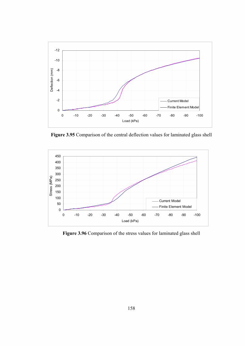
158
-12
-10
-8
-6
-4
-2
0
-100-90-80-70-60-50-40-30-20-100
Load (kPa)
De
flect
ion
(m
m)
Current Model
Finite Element Model
Figure 3.95 Comparison of the central deflection values for laminated glass shell
0
50
100
150
200
250
300
350
400
450
-100-90-80-70-60-50-40-30-20-100
Load (kPa)
Str
ess
(MP
a)
Current Model
Finite Element Model
Figure 3.96 Comparison of the stress values for laminated glass shell
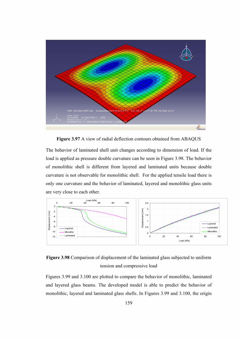
159
Figure 3.97 A view of radial deflection contours obtained from ABAQUS
The behavior of laminated shell unit changes according to dimension of load. If the
load is applied as pressure double curvature can be seen in Figure 3.98. The behavior
of monolithic shell is different from layered and laminated units because double
curvature is not observable for monolithic shell. For the applied tensile load there is
only one curvature and the behavior of laminated, layered and monolithic glass units
are very close to each other.
Figure 3.98 Comparison of displacement of the laminated glass subjected to uniform
tension and compressive load
Figures 3.99 and 3.100 are plotted to compare the behavior of monolithic, laminated
and layered glass beams. The developed model is able to predict the behavior of
monolithic, layered and laminated glass shells. In Figures 3.99 and 3.100, the origin
-12
-10
-8
-6
-4
-2
0
-100-80-60-40-200Load (kPa)
Dis
plac
emen
t (m
m)
Layered
Monolihic
Laminated 0
0,5
1
1,5
2
2,5
0 20 40 60 80 100
Load (kPa)
Dis
palc
emen
t (m
m)
Layered
Laminated
Monolithic
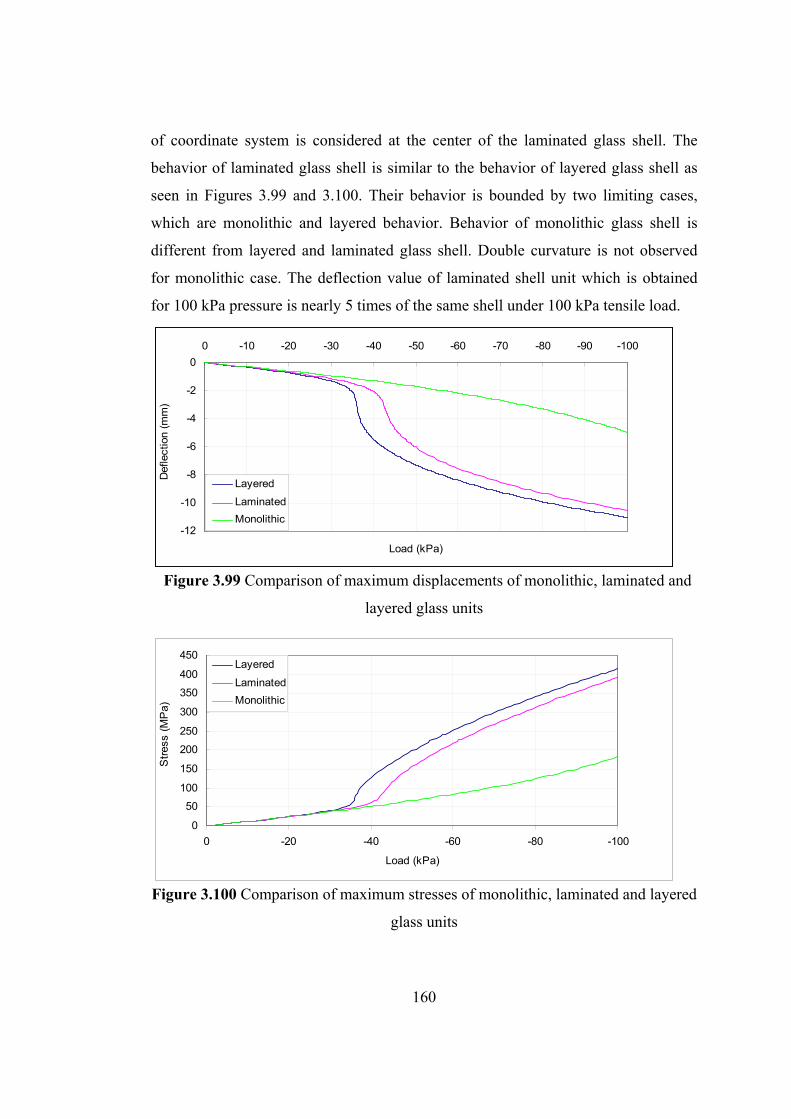
160
of coordinate system is considered at the center of the laminated glass shell. The
behavior of laminated glass shell is similar to the behavior of layered glass shell as
seen in Figures 3.99 and 3.100. Their behavior is bounded by two limiting cases,
which are monolithic and layered behavior. Behavior of monolithic glass shell is
different from layered and laminated glass shell. Double curvature is not observed
for monolithic case. The deflection value of laminated shell unit which is obtained
for 100 kPa pressure is nearly 5 times of the same shell under 100 kPa tensile load.
-12
-10
-8
-6
-4
-2
0
-100-90-80-70-60-50-40-30-20-100
Load (kPa)
Def
lect
ion
(mm
)
Layered
Laminated
Monolithic
Figure 3.99 Comparison of maximum displacements of monolithic, laminated and
layered glass units
0
50
100
150
200
250
300
350
400
450
-100-80-60-40-200
Load (kPa)
Str
ess
(MP
a)
Layered
Laminated
Monolithic
Figure 3.100 Comparison of maximum stresses of monolithic, laminated and layered
glass units
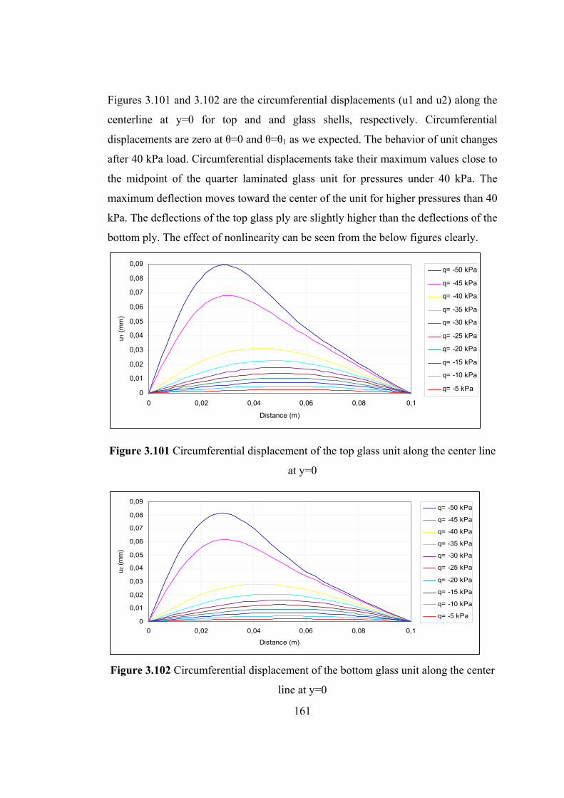
161
Figures 3.101 and 3.102 are the circumferential displacements (u1 and u2) along the
centerline at y=0 for top and and glass shells, respectively. Circumferential
displacements are zero at θ=0 and θ=θ1 as we expected. The behavior of unit changes
after 40 kPa load. Circumferential displacements take their maximum values close to
the midpoint of the quarter laminated glass unit for pressures under 40 kPa. The
maximum deflection moves toward the center of the unit for higher pressures than 40
kPa. The deflections of the top glass ply are slightly higher than the deflections of the
bottom ply. The effect of nonlinearity can be seen from the below figures clearly.
0
0,01
0,02
0,03
0,04
0,05
0,06
0,07
0,08
0,09
0 0,02 0,04 0,06 0,08 0,1
Distance (m)
u1 (
mm
)
q= -50 kPa
q= -45 kPa
q= -40 kPa
q= -35 kPa
q= -30 kPa
q= -25 kPa
q= -20 kPa
q= -15 kPa
q= -10 kPa
q= -5 kPa
Figure 3.101 Circumferential displacement of the top glass unit along the center line
at y=0
0
0,01
0,02
0,03
0,04
0,05
0,06
0,07
0,08
0,09
0 0,02 0,04 0,06 0,08 0,1
Distance (m)
u 2 (
mm
)
q= -50 kPa
q= -45 kPa
q= -40 kPa
q= -35 kPa
q= -30 kPa
q= -25 kPa
q= -20 kPa
q= -15 kPa
q= -10 kPa
q= -5 kPa
Figure 3.102 Circumferential displacement of the bottom glass unit along the center
line at y=0
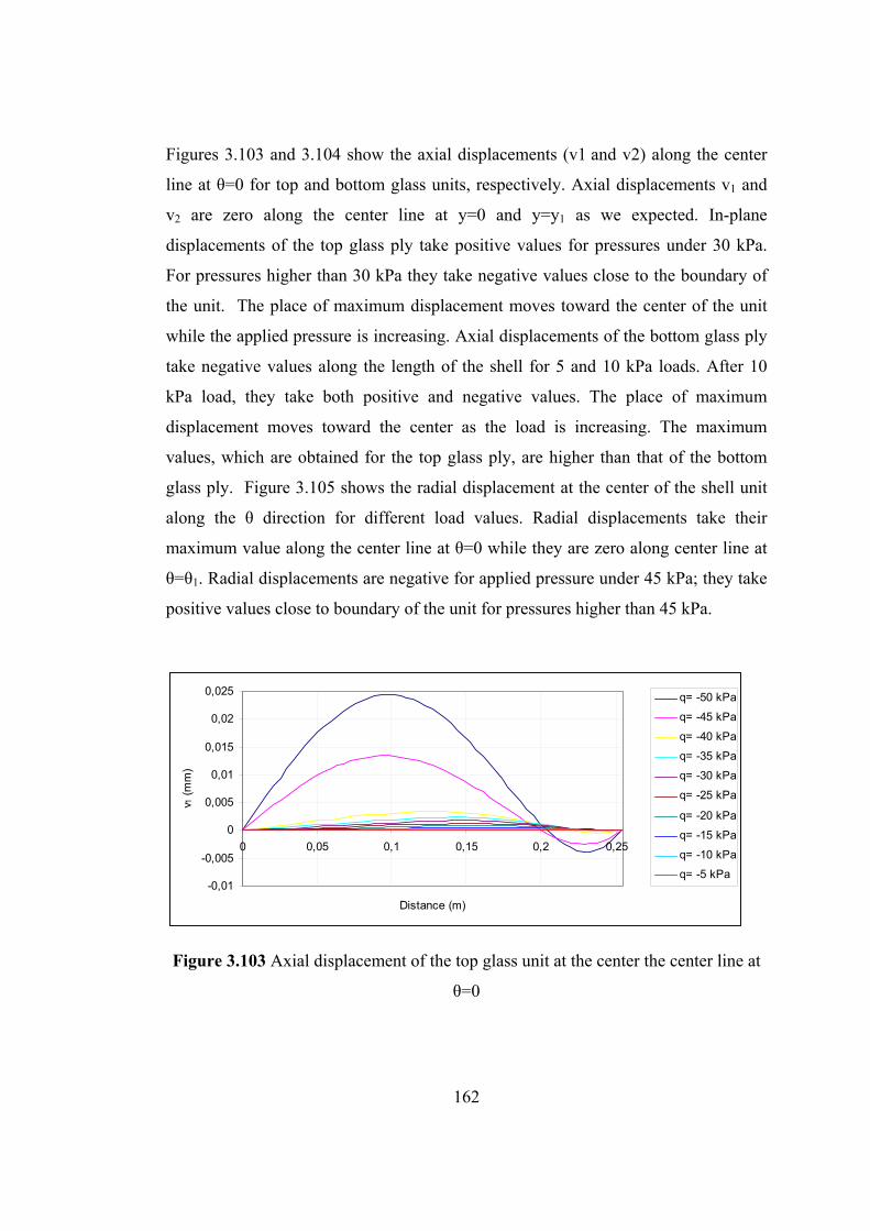
162
Figures 3.103 and 3.104 show the axial displacements (v1 and v2) along the center
line at θ=0 for top and bottom glass units, respectively. Axial displacements v1 and
v2 are zero along the center line at y=0 and y=y1 as we expected. In-plane
displacements of the top glass ply take positive values for pressures under 30 kPa.
For pressures higher than 30 kPa they take negative values close to the boundary of
the unit. The place of maximum displacement moves toward the center of the unit
while the applied pressure is increasing. Axial displacements of the bottom glass ply
take negative values along the length of the shell for 5 and 10 kPa loads. After 10
kPa load, they take both positive and negative values. The place of maximum
displacement moves toward the center as the load is increasing. The maximum
values, which are obtained for the top glass ply, are higher than that of the bottom
glass ply. Figure 3.105 shows the radial displacement at the center of the shell unit
along the θ direction for different load values. Radial displacements take their
maximum value along the center line at θ=0 while they are zero along center line at
θ=θ1. Radial displacements are negative for applied pressure under 45 kPa; they take
positive values close to boundary of the unit for pressures higher than 45 kPa.
-0,01
-0,005
0
0,005
0,01
0,015
0,02
0,025
0 0,05 0,1 0,15 0,2 0,25
Distance (m)
v1 (
mm
)
q= -50 kPa
q= -45 kPa
q= -40 kPa
q= -35 kPa
q= -30 kPa
q= -25 kPa
q= -20 kPa
q= -15 kPa
q= -10 kPa
q= -5 kPa
Figure 3.103 Axial displacement of the top glass unit at the center the center line at
θ=0
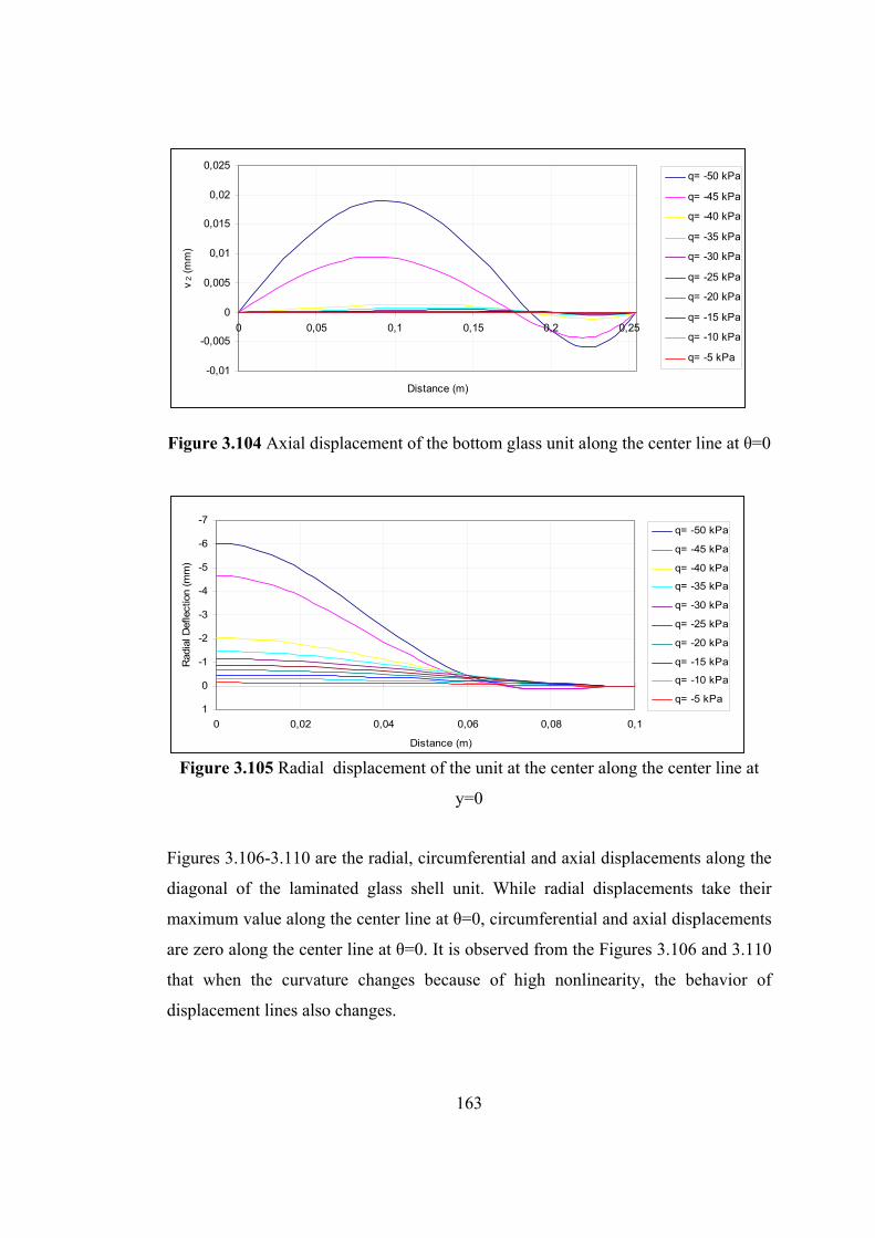
163
-0,01
-0,005
0
0,005
0,01
0,015
0,02
0,025
0 0,05 0,1 0,15 0,2 0,25
Distance (m)
v 2
(mm
)q= -50 kPa
q= -45 kPa
q= -40 kPa
q= -35 kPa
q= -30 kPa
q= -25 kPa
q= -20 kPa
q= -15 kPa
q= -10 kPa
q= -5 kPa
Figure 3.104 Axial displacement of the bottom glass unit along the center line at θ=0
-7
-6
-5
-4
-3
-2
-1
0
1
0 0,02 0,04 0,06 0,08 0,1
Distance (m)
Rad
ial D
efle
ctio
n (m
m)
q= -50 kPa
q= -45 kPa
q= -40 kPa
q= -35 kPa
q= -30 kPa
q= -25 kPa
q= -20 kPa
q= -15 kPa
q= -10 kPa
q= -5 kPa
Figure 3.105 Radial displacement of the unit at the center along the center line at
y=0
Figures 3.106-3.110 are the radial, circumferential and axial displacements along the
diagonal of the laminated glass shell unit. While radial displacements take their
maximum value along the center line at θ=0, circumferential and axial displacements
are zero along the center line at θ=0. It is observed from the Figures 3.106 and 3.110
that when the curvature changes because of high nonlinearity, the behavior of
displacement lines also changes.
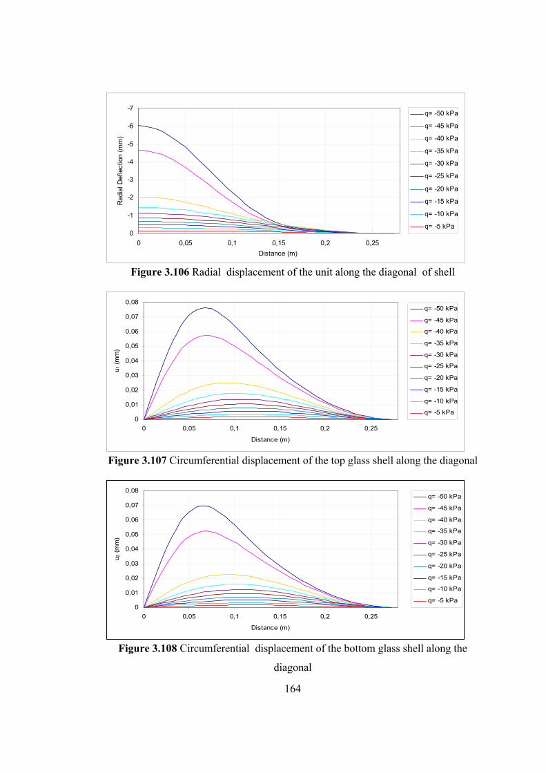
164
-7
-6
-5
-4
-3
-2
-1
0
0 0,05 0,1 0,15 0,2 0,25
Distance (m)
Rad
ial D
efle
ctio
n (m
m)
q= -50 kPa
q= -45 kPa
q= -40 kPa
q= -35 kPa
q= -30 kPa
q= -25 kPa
q= -20 kPa
q= -15 kPa
q= -10 kPa
q= -5 kPa
Figure 3.106 Radial displacement of the unit along the diagonal of shell
0
0,01
0,02
0,03
0,04
0,05
0,06
0,07
0,08
0 0,05 0,1 0,15 0,2 0,25
Distance (m)
u 1 (
mm
)
q= -50 kPa
q= -45 kPa
q= -40 kPa
q= -35 kPa
q= -30 kPa
q= -25 kPa
q= -20 kPa
q= -15 kPa
q= -10 kPa
q= -5 kPa
Figure 3.107 Circumferential displacement of the top glass shell along the diagonal
0
0,01
0,02
0,03
0,04
0,05
0,06
0,07
0,08
0 0,05 0,1 0,15 0,2 0,25
Distance (m)
u 2 (
mm
)
q= -50 kPa
q= -45 kPa
q= -40 kPa
q= -35 kPa
q= -30 kPa
q= -25 kPa
q= -20 kPa
q= -15 kPa
q= -10 kPa
q= -5 kPa
Figure 3.108 Circumferential displacement of the bottom glass shell along the
diagonal
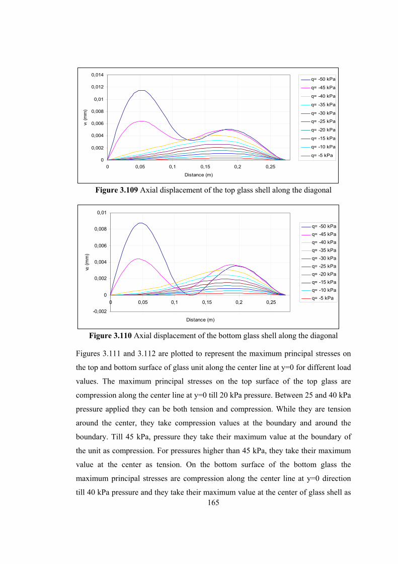
165
0
0,002
0,004
0,006
0,008
0,01
0,012
0,014
0 0,05 0,1 0,15 0,2 0,25
Distance (m)
v 1 (
mm
)q= -50 kPa
q= -45 kPa
q= -40 kPa
q= -35 kPa
q= -30 kPa
q= -25 kPa
q= -20 kPa
q= -15 kPa
q= -10 kPa
q= -5 kPa
Figure 3.109 Axial displacement of the top glass shell along the diagonal
-0,002
0
0,002
0,004
0,006
0,008
0,01
0 0,05 0,1 0,15 0,2 0,25
Distance (m)
v2 (
mm
)
q= -50 kPa
q= -45 kPa
q= -40 kPa
q= -35 kPa
q= -30 kPa
q= -25 kPa
q= -20 kPa
q= -15 kPa
q= -10 kPa
q= -5 kPa
Figure 3.110 Axial displacement of the bottom glass shell along the diagonal
Figures 3.111 and 3.112 are plotted to represent the maximum principal stresses on
the top and bottom surface of glass unit along the center line at y=0 for different load
values. The maximum principal stresses on the top surface of the top glass are
compression along the center line at y=0 till 20 kPa pressure. Between 25 and 40 kPa
pressure applied they can be both tension and compression. While they are tension
around the center, they take compression values at the boundary and around the
boundary. Till 45 kPa, pressure they take their maximum value at the boundary of
the unit as compression. For pressures higher than 45 kPa, they take their maximum
value at the center as tension. On the bottom surface of the bottom glass the
maximum principal stresses are compression along the center line at y=0 direction
till 40 kPa pressure and they take their maximum value at the center of glass shell as
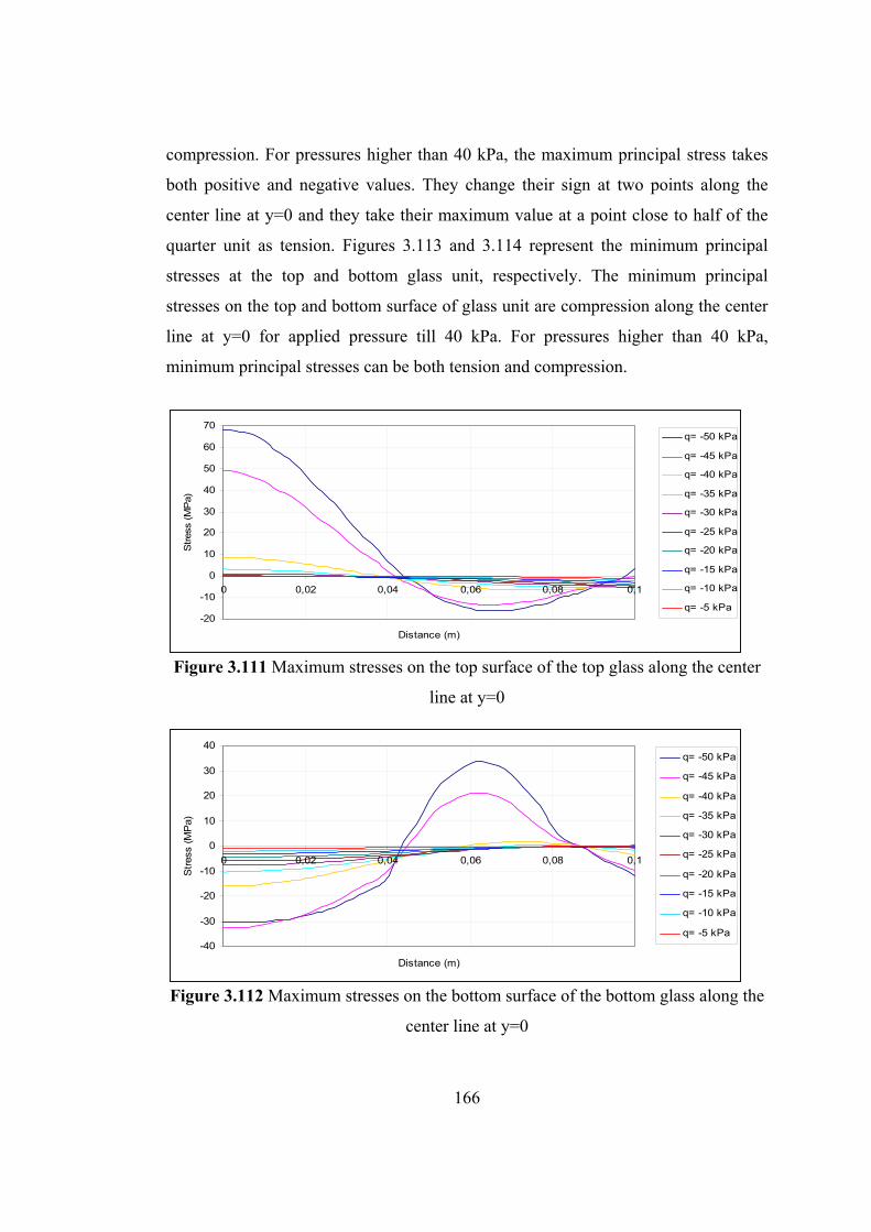
166
compression. For pressures higher than 40 kPa, the maximum principal stress takes
both positive and negative values. They change their sign at two points along the
center line at y=0 and they take their maximum value at a point close to half of the
quarter unit as tension. Figures 3.113 and 3.114 represent the minimum principal
stresses at the top and bottom glass unit, respectively. The minimum principal
stresses on the top and bottom surface of glass unit are compression along the center
line at y=0 for applied pressure till 40 kPa. For pressures higher than 40 kPa,
minimum principal stresses can be both tension and compression.
-20
-10
0
10
20
30
40
50
60
70
0 0,02 0,04 0,06 0,08 0,1
Distance (m)
Stres
s (M
Pa)
q= -50 kPa
q= -45 kPa
q= -40 kPa
q= -35 kPa
q= -30 kPa
q= -25 kPa
q= -20 kPa
q= -15 kPa
q= -10 kPa
q= -5 kPa
Figure 3.111 Maximum stresses on the top surface of the top glass along the center
line at y=0
-40
-30
-20
-10
0
10
20
30
40
0 0,02 0,04 0,06 0,08 0,1
Distance (m)
Str
ess
(MP
a)
q= -50 kPa
q= -45 kPa
q= -40 kPa
q= -35 kPa
q= -30 kPa
q= -25 kPa
q= -20 kPa
q= -15 kPa
q= -10 kPa
q= -5 kPa
Figure 3.112 Maximum stresses on the bottom surface of the bottom glass along the
center line at y=0
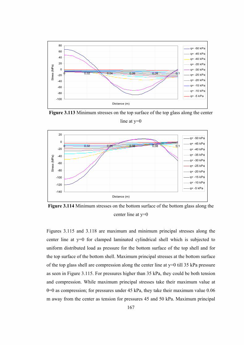
167
-100
-80
-60
-40
-20
0
20
40
60
80
0 0,02 0,04 0,06 0,08 0,1
Distance (m)
Stres
s (M
Pa)
q= -50 kPa
q= -45 kPa
q= -40 kPa
q= -35 kPa
q= -30 kPa
q= -25 kPa
q= -20 kPa
q= -15 kPa
q= -10 kPa
q= -5 kPa
Figure 3.113 Minimum stresses on the top surface of the top glass along the center
line at y=0
-140
-120
-100
-80
-60
-40
-20
0
20
0 0,02 0,04 0,06 0,08 0,1
Distance (m)
Str
ess
(MP
a)
q= -50 kPa
q= -45 kPa
q= -40 kPa
q= -35 kPa
q= -30 kPa
q= -25 kPa
q= -20 kPa
q= -15 kPa
q= -10 kPa
q= -5 kPa
Figure 3.114 Minimum stresses on the bottom surface of the bottom glass along the
center line at y=0
Figures 3.115 and 3.118 are maximum and minimum principal stresses along the
center line at y=0 for clamped laminated cylindrical shell which is subjected to
uniform distributed load as pressure for the bottom surface of the top shell and for
the top surface of the bottom shell. Maximum principal stresses at the bottom surface
of the top glass shell are compression along the center line at y=0 till 35 kPa pressure
as seen in Figure 3.115. For pressures higher than 35 kPa, they could be both tension
and compression. While maximum principal stresses take their maximum value at
θ=0 as compression; for pressures under 45 kPa, they take their maximum value 0.06
m away from the center as tension for pressures 45 and 50 kPa. Maximum principal
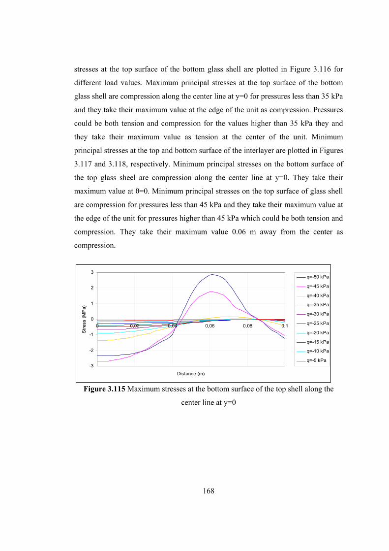
168
stresses at the top surface of the bottom glass shell are plotted in Figure 3.116 for
different load values. Maximum principal stresses at the top surface of the bottom
glass shell are compression along the center line at y=0 for pressures less than 35 kPa
and they take their maximum value at the edge of the unit as compression. Pressures
could be both tension and compression for the values higher than 35 kPa they and
they take their maximum value as tension at the center of the unit. Minimum
principal stresses at the top and bottom surface of the interlayer are plotted in Figures
3.117 and 3.118, respectively. Minimum principal stresses on the bottom surface of
the top glass sheel are compression along the center line at y=0. They take their
maximum value at θ=0. Minimum principal stresses on the top surface of glass shell
are compression for pressures less than 45 kPa and they take their maximum value at
the edge of the unit for pressures higher than 45 kPa which could be both tension and
compression. They take their maximum value 0.06 m away from the center as
compression.
-3
-2
-1
0
1
2
3
0 0,02 0,04 0,06 0,08 0,1
Distance (m)
Str
ess
(MP
a)
q=-50 kPa
q=-45 kPa
q=-40 kPa
q=-35 kPa
q=-30 kPa
q=-25 kPa
q=-20 kPa
q=-15 kPa
q=-10 kPa
q=-5 kPa
Figure 3.115 Maximum stresses at the bottom surface of the top shell along the
center line at y=0
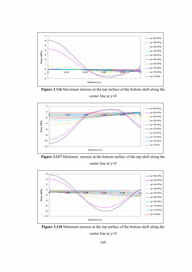
169
-2
-1
0
1
2
3
4
5
6
7
0 0,02 0,04 0,06 0,08 0,1
Distance (m)
Stres
s (M
Pa)
q=-50 kPa
q=-45 kPa
q=-40 kPa
q=-35 kPa
q=-30 kPa
q=-25 kPa
q=-20 kPa
q=-15 kPa
q=-10 kPa
q=-5 kPa
Figure 3.116 Maximum stresses at the top surface of the bottom shell along the
center line at y=0
-12
-10
-8
-6
-4
-2
0
2
0 0,02 0,04 0,06 0,08 0,1
Distance (m)
Stres
s (M
Pa)
q=-50 kPa
q=-45 kPa
q=-40 kPa
q=-35 kPa
q=-30 kPa
q=-25 kPa
q=-20 kPa
q=-15 kPa
q=-10 kPa
q=-5 kPa
Figure 3.117 Minimum stresses at the bottom surface of the top shell along the
center line at y=0
-10
-8
-6
-4
-2
0
2
4
6
0 0,02 0,04 0,06 0,08 0,1
Distance (m)
Stres
s (M
Pa)
q=-50 kPa
q=-45 kPa
q=-40 kPa
q=-35 kPa
q=-30 kPa
q=-25 kPa
q=-20 kPa
q=-15 kPa
q=-10 kPa
q=-5 kPa
Figure 3.118 Minimum stresses at the top surface of the bottom shell along the
center line at y=0
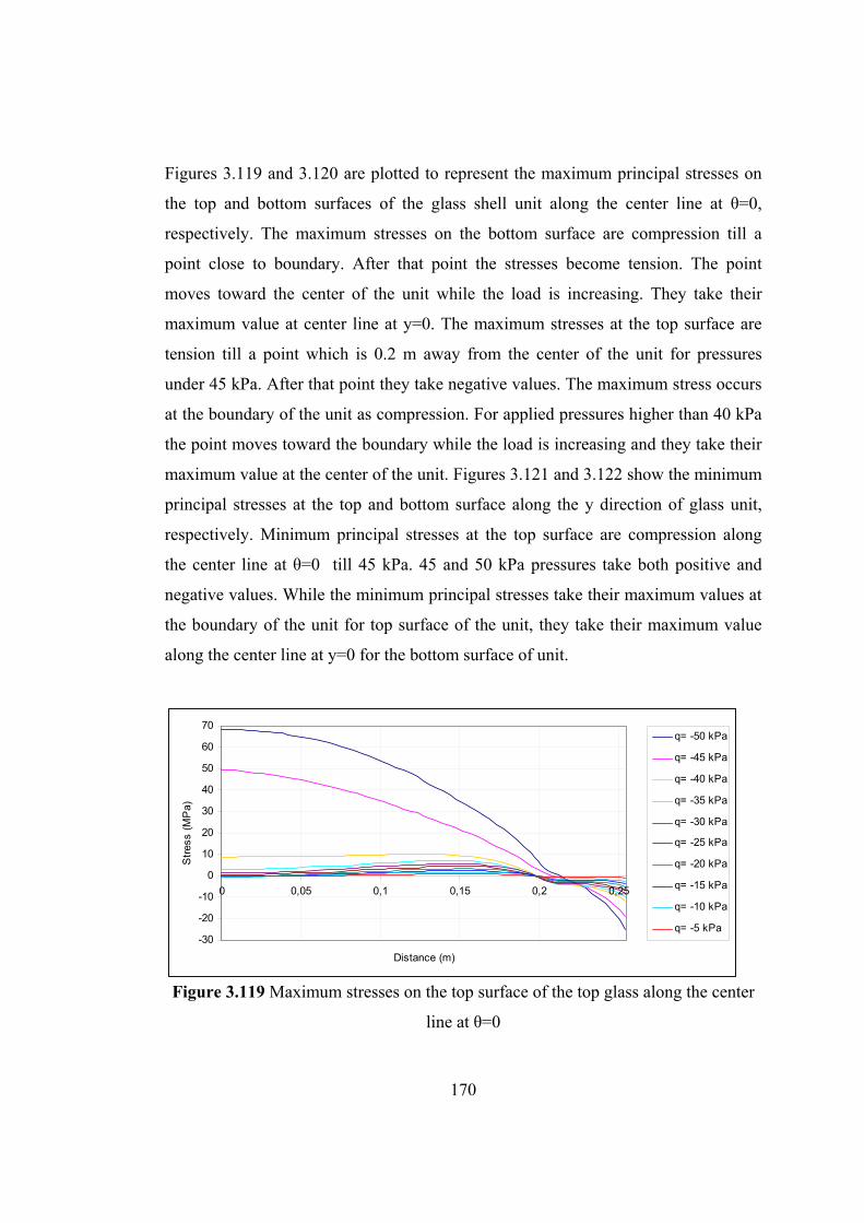
170
Figures 3.119 and 3.120 are plotted to represent the maximum principal stresses on
the top and bottom surfaces of the glass shell unit along the center line at θ=0,
respectively. The maximum stresses on the bottom surface are compression till a
point close to boundary. After that point the stresses become tension. The point
moves toward the center of the unit while the load is increasing. They take their
maximum value at center line at y=0. The maximum stresses at the top surface are
tension till a point which is 0.2 m away from the center of the unit for pressures
under 45 kPa. After that point they take negative values. The maximum stress occurs
at the boundary of the unit as compression. For applied pressures higher than 40 kPa
the point moves toward the boundary while the load is increasing and they take their
maximum value at the center of the unit. Figures 3.121 and 3.122 show the minimum
principal stresses at the top and bottom surface along the y direction of glass unit,
respectively. Minimum principal stresses at the top surface are compression along
the center line at θ=0 till 45 kPa. 45 and 50 kPa pressures take both positive and
negative values. While the minimum principal stresses take their maximum values at
the boundary of the unit for top surface of the unit, they take their maximum value
along the center line at y=0 for the bottom surface of unit.
-30
-20
-10
0
10
20
30
40
50
60
70
0 0,05 0,1 0,15 0,2 0,25
Distance (m)
Str
ess
(MP
a)
q= -50 kPa
q= -45 kPa
q= -40 kPa
q= -35 kPa
q= -30 kPa
q= -25 kPa
q= -20 kPa
q= -15 kPa
q= -10 kPa
q= -5 kPa
Figure 3.119 Maximum stresses on the top surface of the top glass along the center
line at θ=0
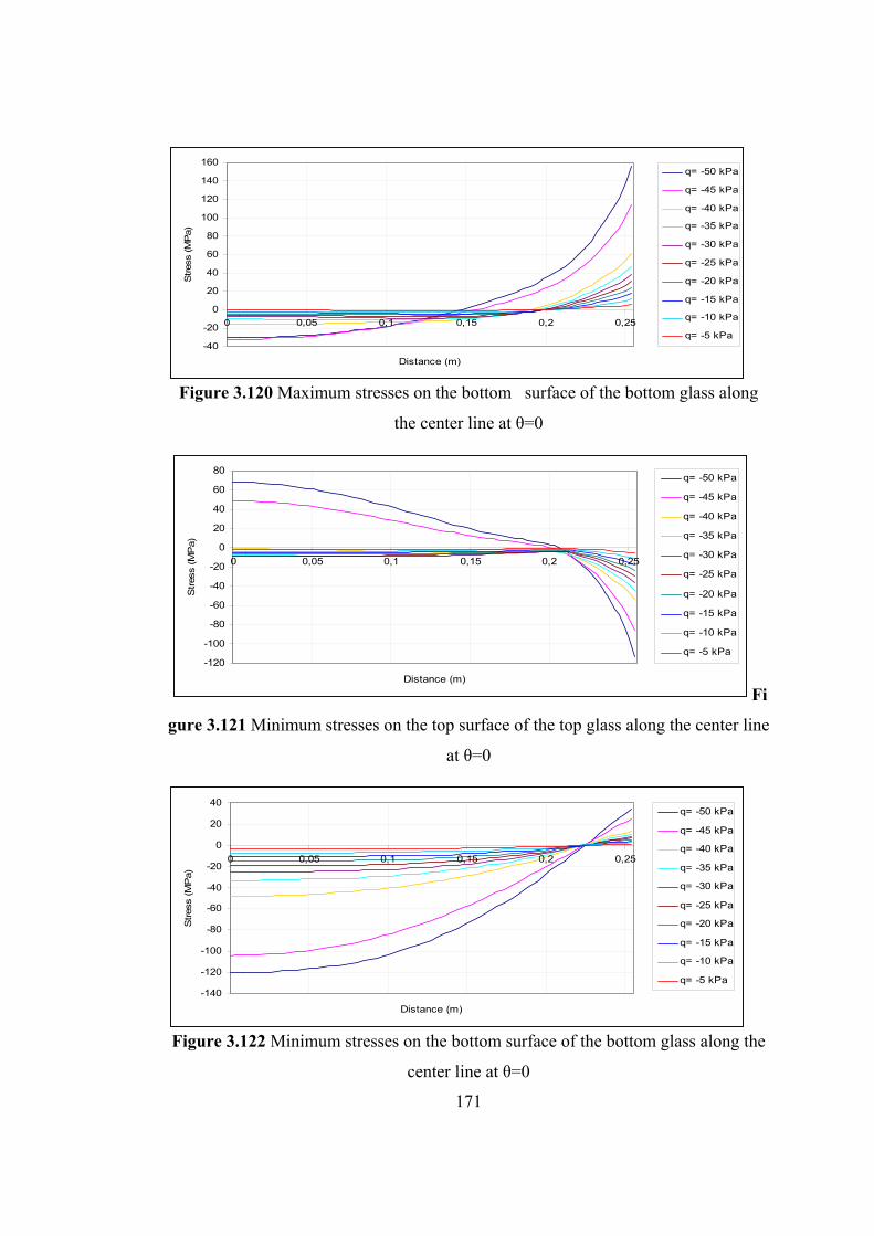
171
-40
-20
0
20
40
60
80
100
120
140
160
0 0,05 0,1 0,15 0,2 0,25
Distance (m)
Stres
s (M
Pa)
q= -50 kPa
q= -45 kPa
q= -40 kPa
q= -35 kPa
q= -30 kPa
q= -25 kPa
q= -20 kPa
q= -15 kPa
q= -10 kPa
q= -5 kPa
Figure 3.120 Maximum stresses on the bottom surface of the bottom glass along
the center line at θ=0
-120
-100
-80
-60
-40
-20
0
20
40
60
80
0 0,05 0,1 0,15 0,2 0,25
Distance (m)
Stres
s (M
Pa)
q= -50 kPa
q= -45 kPa
q= -40 kPa
q= -35 kPa
q= -30 kPa
q= -25 kPa
q= -20 kPa
q= -15 kPa
q= -10 kPa
q= -5 kPa
Fi
gure 3.121 Minimum stresses on the top surface of the top glass along the center line
at θ=0
-140
-120
-100
-80
-60
-40
-20
0
20
40
0 0,05 0,1 0,15 0,2 0,25
Distance (m)
Stres
s (M
Pa)
q= -50 kPa
q= -45 kPa
q= -40 kPa
q= -35 kPa
q= -30 kPa
q= -25 kPa
q= -20 kPa
q= -15 kPa
q= -10 kPa
q= -5 kPa
Figure 3.122 Minimum stresses on the bottom surface of the bottom glass along the
center line at θ=0
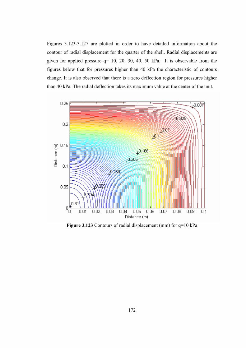
172
Figures 3.123-3.127 are plotted in order to have detailed information about the
contour of radial displacement for the quarter of the shell. Radial displacements are
given for applied pressure q= 10, 20, 30, 40, 50 kPa. It is observable from the
figures below that for pressures higher than 40 kPa the characteristic of contours
change. It is also observed that there is a zero deflection region for pressures higher
than 40 kPa. The radial deflection takes its maximum value at the center of the unit.
Figure 3.123 Contours of radial displacement (mm) for q=10 kPa
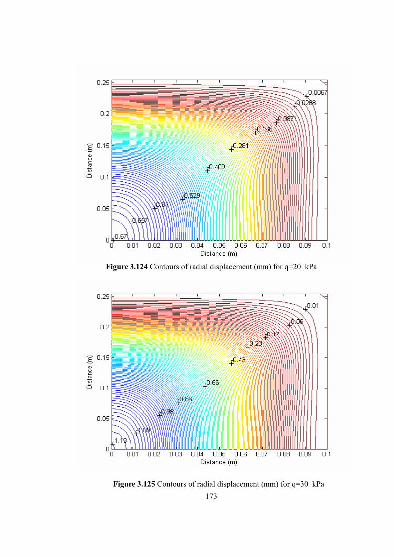
173
Figure 3.124 Contours of radial displacement (mm) for q=20 kPa
Figure 3.125 Contours of radial displacement (mm) for q=30 kPa
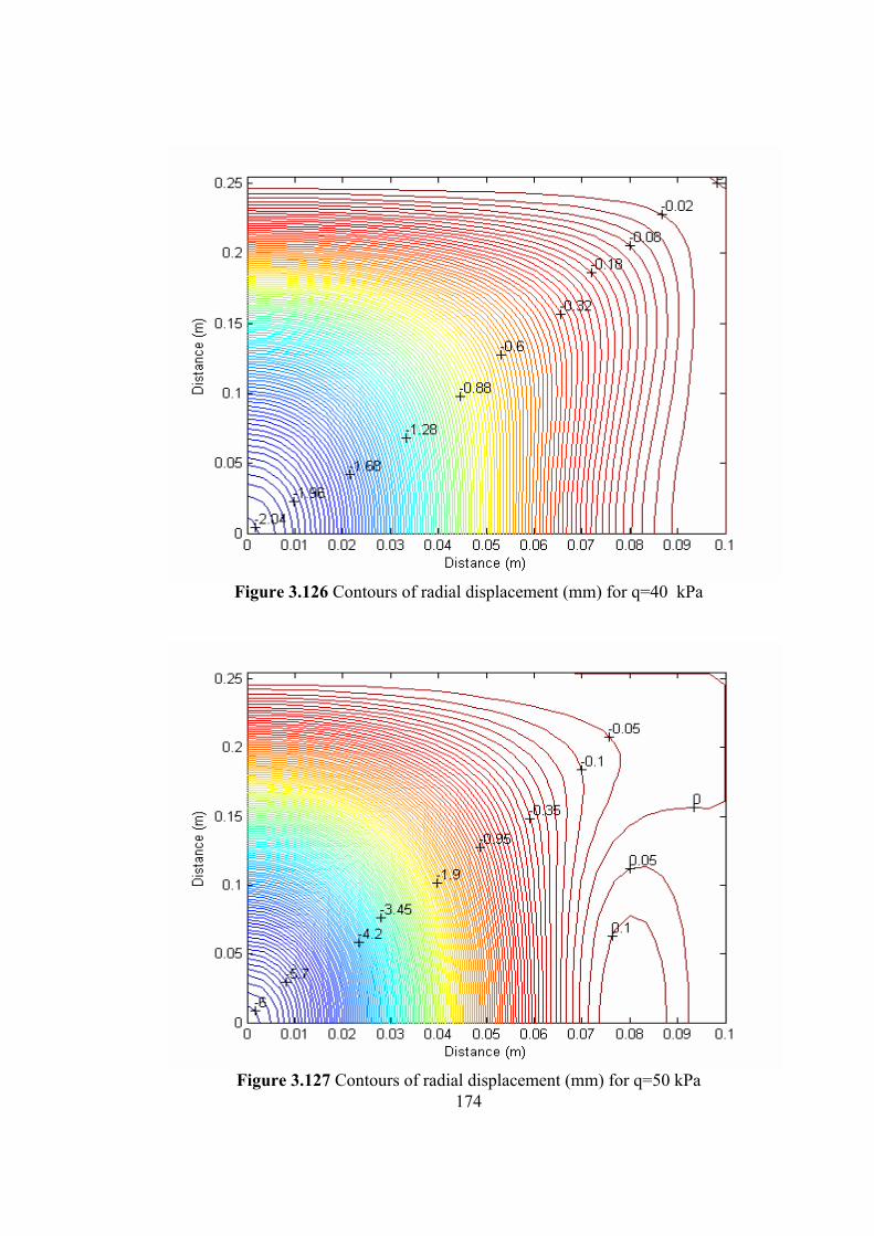
174
Figure 3.126 Contours of radial displacement (mm) for q=40 kPa
Figure 3.127 Contours of radial displacement (mm) for q=50 kPa
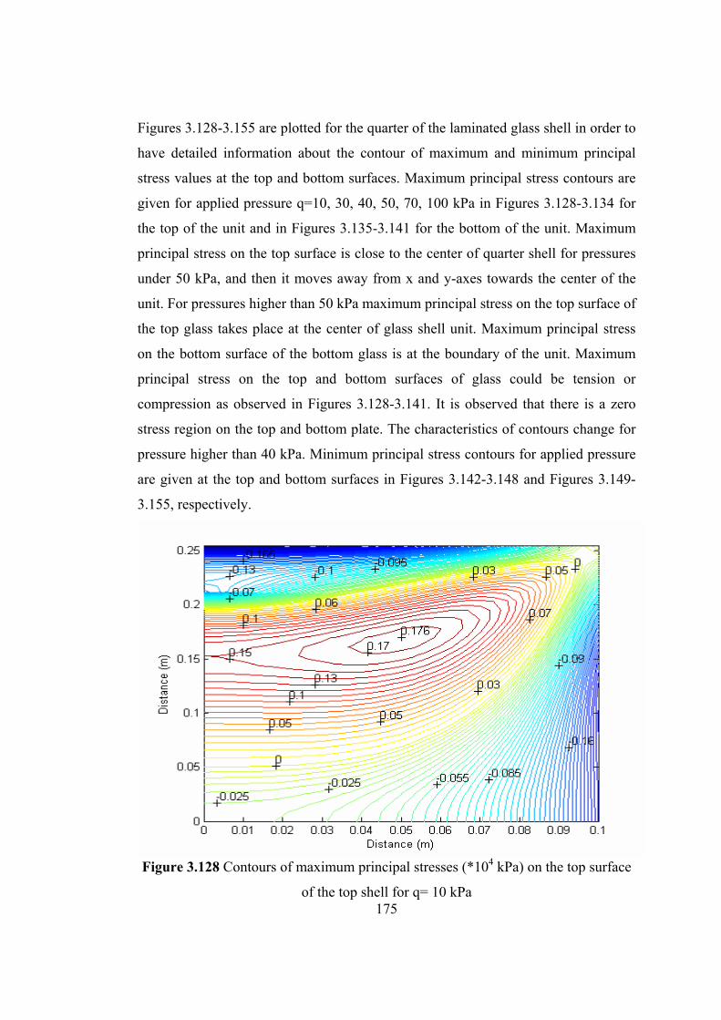
175
Figures 3.128-3.155 are plotted for the quarter of the laminated glass shell in order to
have detailed information about the contour of maximum and minimum principal
stress values at the top and bottom surfaces. Maximum principal stress contours are
given for applied pressure q=10, 30, 40, 50, 70, 100 kPa in Figures 3.128-3.134 for
the top of the unit and in Figures 3.135-3.141 for the bottom of the unit. Maximum
principal stress on the top surface is close to the center of quarter shell for pressures
under 50 kPa, and then it moves away from x and y-axes towards the center of the
unit. For pressures higher than 50 kPa maximum principal stress on the top surface of
the top glass takes place at the center of glass shell unit. Maximum principal stress
on the bottom surface of the bottom glass is at the boundary of the unit. Maximum
principal stress on the top and bottom surfaces of glass could be tension or
compression as observed in Figures 3.128-3.141. It is observed that there is a zero
stress region on the top and bottom plate. The characteristics of contours change for
pressure higher than 40 kPa. Minimum principal stress contours for applied pressure
are given at the top and bottom surfaces in Figures 3.142-3.148 and Figures 3.149-
3.155, respectively.
Figure 3.128 Contours of maximum principal stresses (*104 kPa) on the top surface
of the top shell for q= 10 kPa
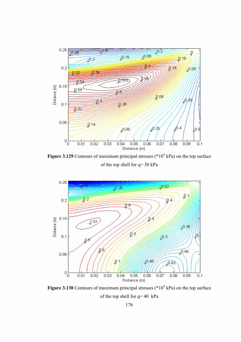
176
Figure 3.129 Contours of maximum principal stresses (*104 kPa) on the top surface
of the top shell for q= 30 kPa
Figure 3.130 Contours of maximum principal stresses (*104 kPa) on the top surface
of the top shell for q= 40 kPa
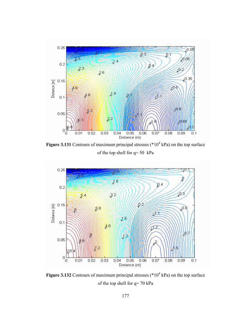
177
Figure 3.131 Contours of maximum principal stresses (*104 kPa) on the top surface
of the top shell for q= 50 kPa
Figure 3.132 Contours of maximum principal stresses (*104 kPa) on the top surface
of the top shell for q= 70 kPa
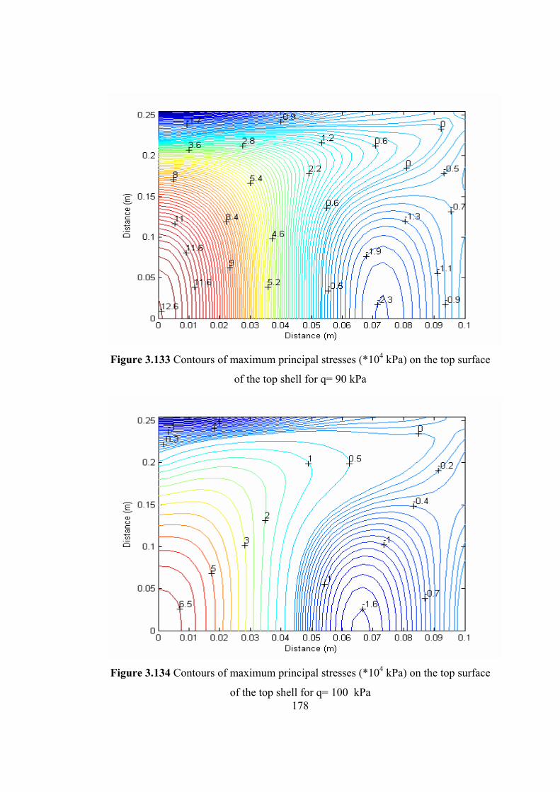
178
Figure 3.133 Contours of maximum principal stresses (*104 kPa) on the top surface
of the top shell for q= 90 kPa
Figure 3.134 Contours of maximum principal stresses (*104 kPa) on the top surface
of the top shell for q= 100 kPa
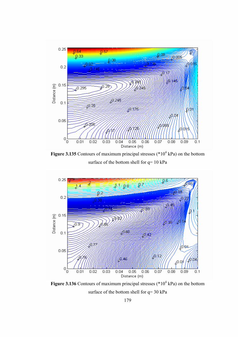
179
Figure 3.135 Contours of maximum principal stresses (*104 kPa) on the bottom
surface of the bottom shell for q= 10 kPa
Figure 3.136 Contours of maximum principal stresses (*104 kPa) on the bottom
surface of the bottom shell for q= 30 kPa
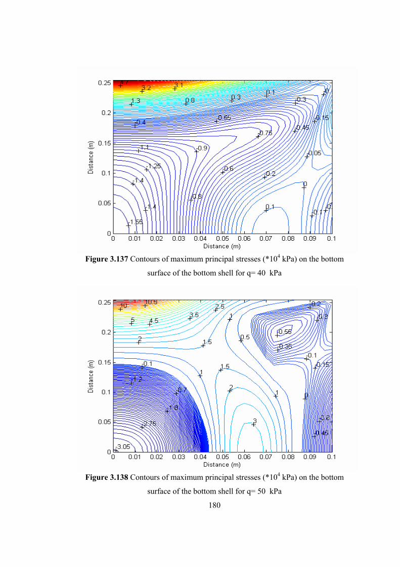
180
Figure 3.137 Contours of maximum principal stresses (*104 kPa) on the bottom
surface of the bottom shell for q= 40 kPa
Figure 3.138 Contours of maximum principal stresses (*104 kPa) on the bottom
surface of the bottom shell for q= 50 kPa
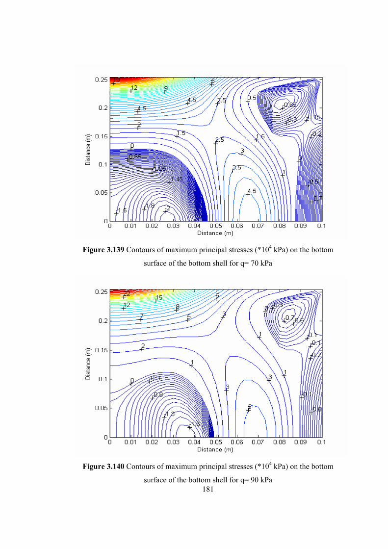
181
Figure 3.139 Contours of maximum principal stresses (*104 kPa) on the bottom
surface of the bottom shell for q= 70 kPa
Figure 3.140 Contours of maximum principal stresses (*104 kPa) on the bottom
surface of the bottom shell for q= 90 kPa
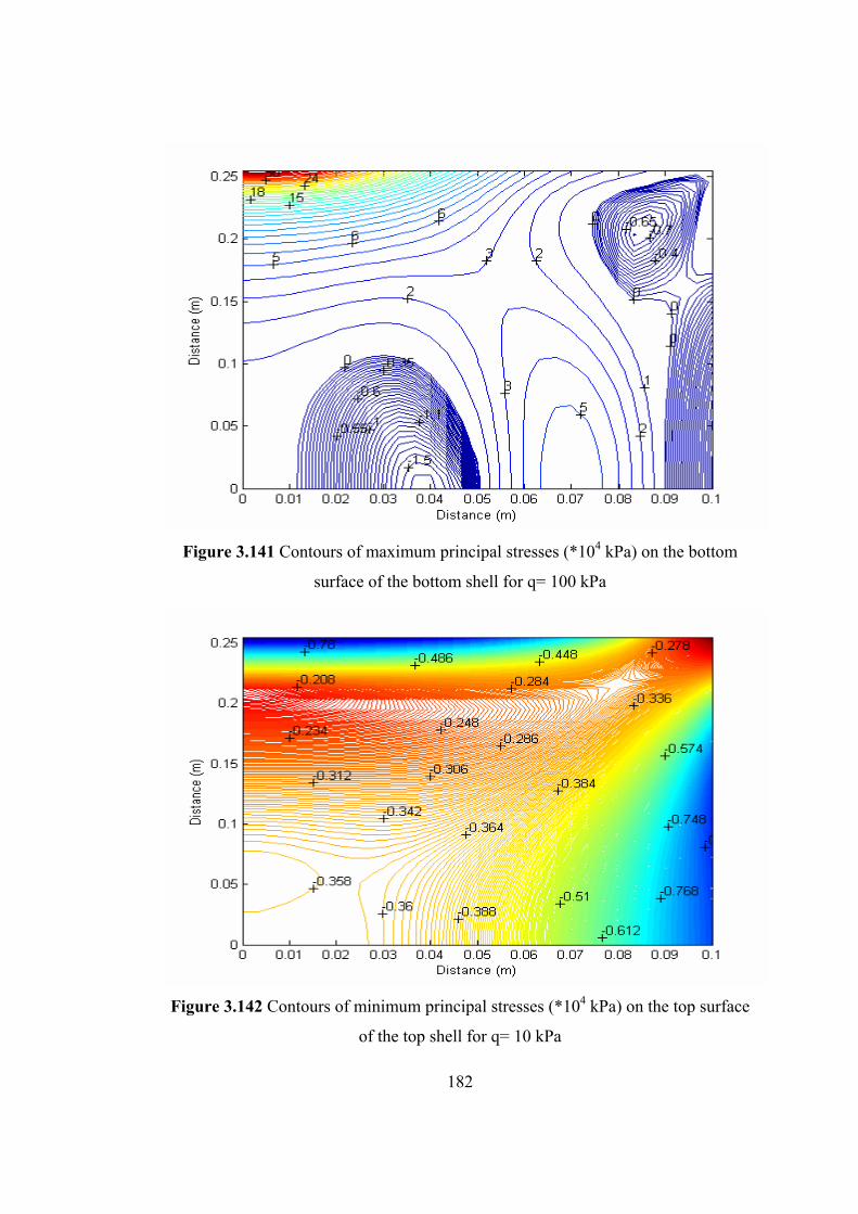
182
Figure 3.141 Contours of maximum principal stresses (*104 kPa) on the bottom
surface of the bottom shell for q= 100 kPa
Figure 3.142 Contours of minimum principal stresses (*104 kPa) on the top surface
of the top shell for q= 10 kPa
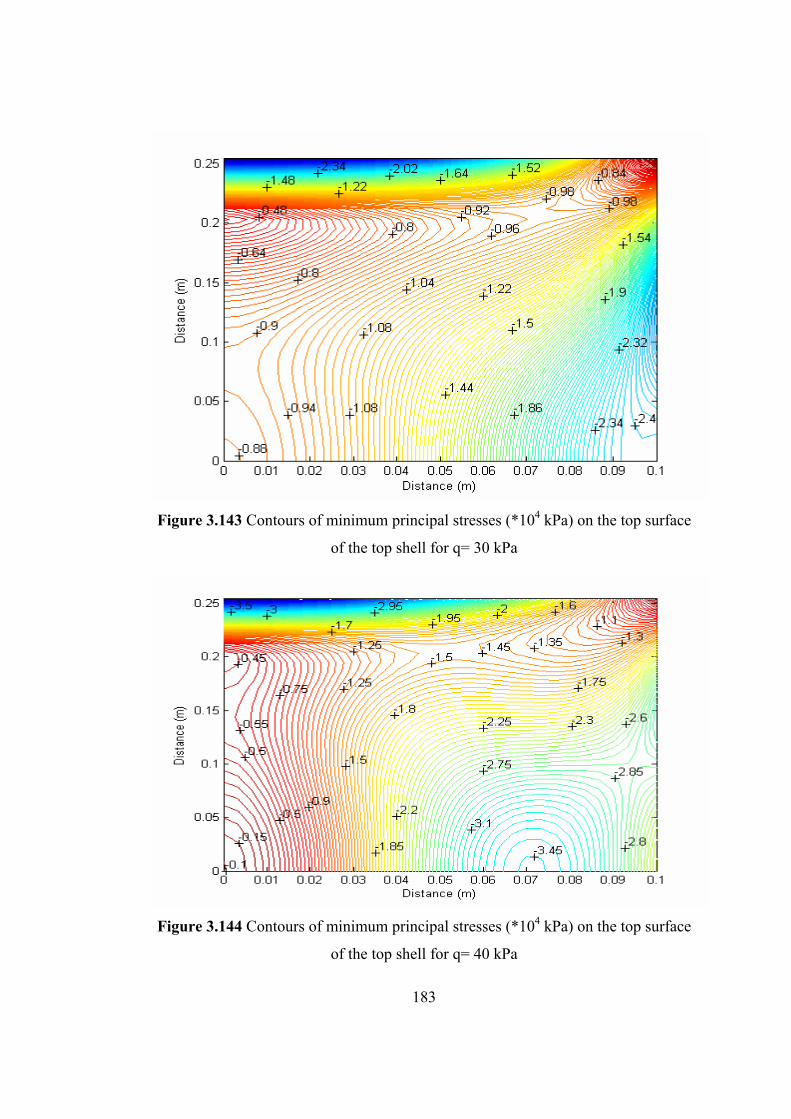
183
Figure 3.143 Contours of minimum principal stresses (*104 kPa) on the top surface
of the top shell for q= 30 kPa
Figure 3.144 Contours of minimum principal stresses (*104 kPa) on the top surface
of the top shell for q= 40 kPa
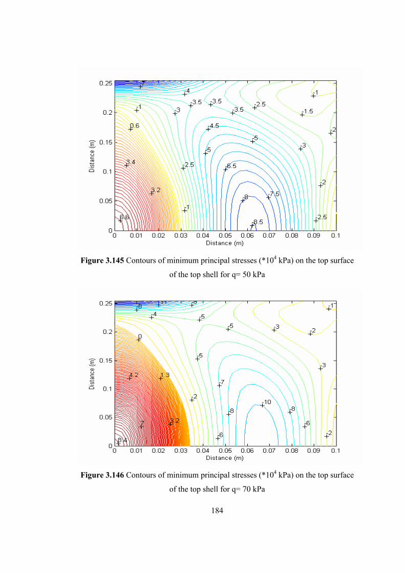
184
Figure 3.145 Contours of minimum principal stresses (*104 kPa) on the top surface
of the top shell for q= 50 kPa
Figure 3.146 Contours of minimum principal stresses (*104 kPa) on the top surface
of the top shell for q= 70 kPa
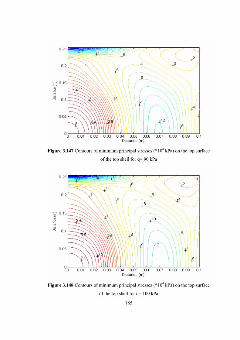
185
Figure 3.147 Contours of minimum principal stresses (*104 kPa) on the top surface
of the top shell for q= 90 kPa
Figure 3.148 Contours of minimum principal stresses (*104 kPa) on the top surface
of the top shell for q= 100 kPa
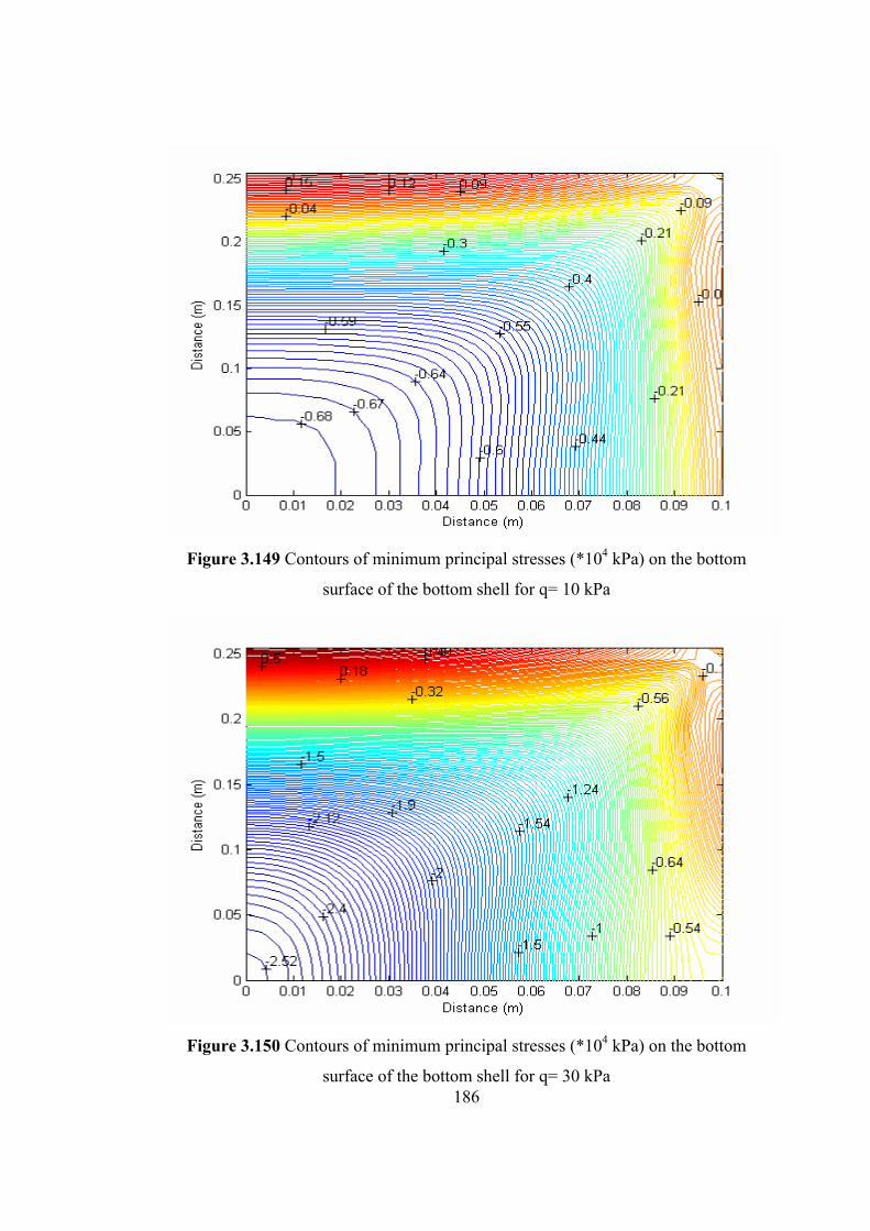
186
Figure 3.149 Contours of minimum principal stresses (*104 kPa) on the bottom
surface of the bottom shell for q= 10 kPa
Figure 3.150 Contours of minimum principal stresses (*104 kPa) on the bottom
surface of the bottom shell for q= 30 kPa
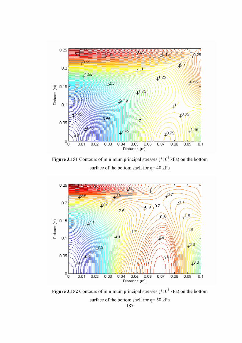
187
Figure 3.151 Contours of minimum principal stresses (*104 kPa) on the bottom
surface of the bottom shell for q= 40 kPa
Figure 3.152 Contours of minimum principal stresses (*104 kPa) on the bottom
surface of the bottom shell for q= 50 kPa
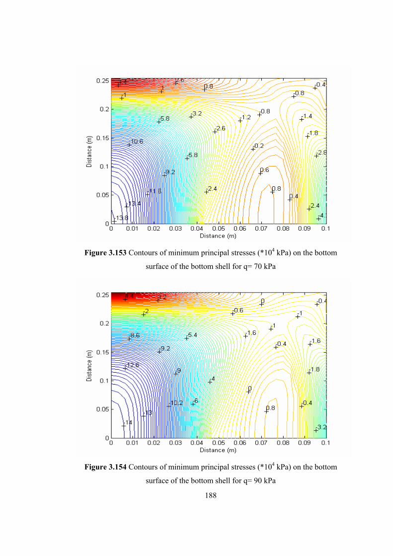
188
Figure 3.153 Contours of minimum principal stresses (*104 kPa) on the bottom
surface of the bottom shell for q= 70 kPa
Figure 3.154 Contours of minimum principal stresses (*104 kPa) on the bottom
surface of the bottom shell for q= 90 kPa
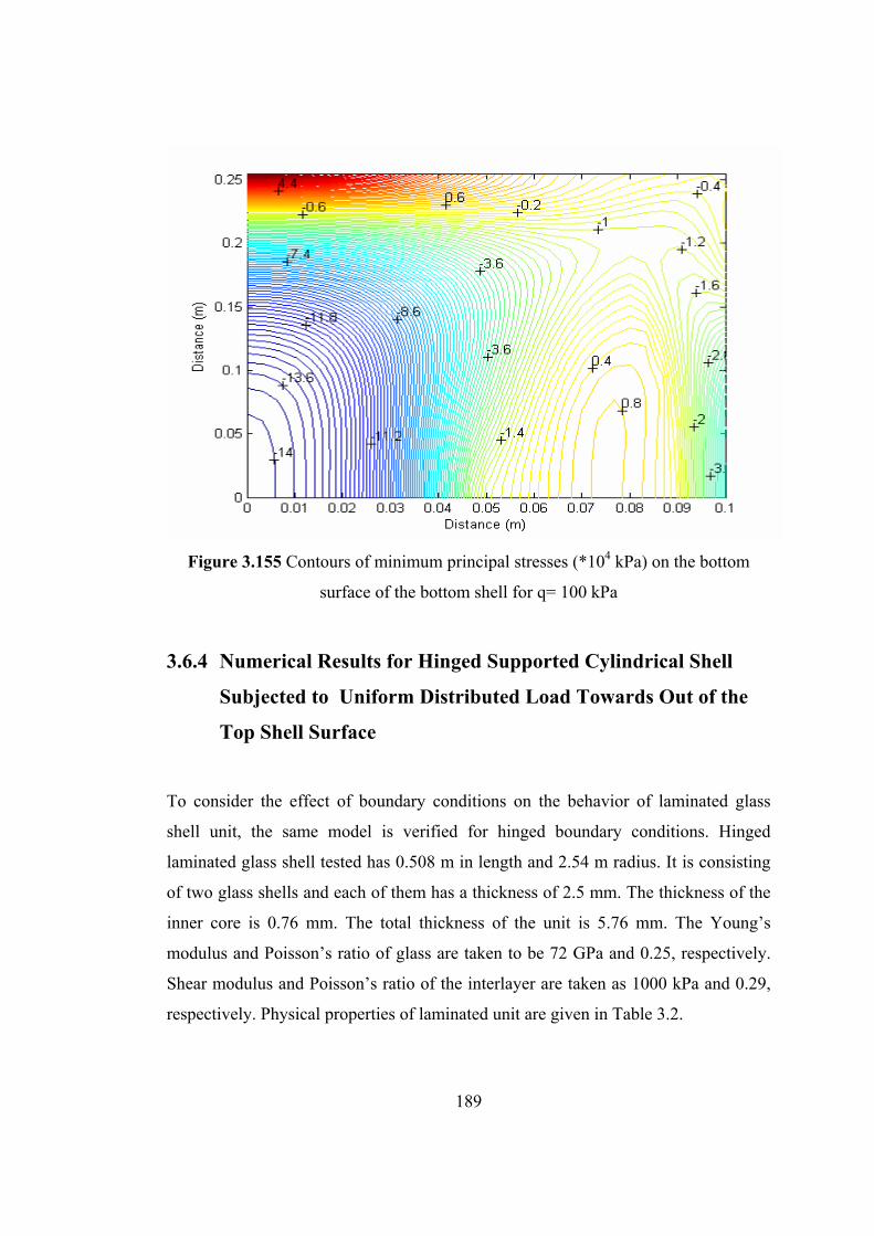
189
Figure 3.155 Contours of minimum principal stresses (*104 kPa) on the bottom
surface of the bottom shell for q= 100 kPa
3.6.4 Numerical Results for Hinged Supported Cylindrical Shell
Subjected to Uniform Distributed Load Towards Out of the
Top Shell Surface
To consider the effect of boundary conditions on the behavior of laminated glass
shell unit, the same model is verified for hinged boundary conditions. Hinged
laminated glass shell tested has 0.508 m in length and 2.54 m radius. It is consisting
of two glass shells and each of them has a thickness of 2.5 mm. The thickness of the
inner core is 0.76 mm. The total thickness of the unit is 5.76 mm. The Young’s
modulus and Poisson’s ratio of glass are taken to be 72 GPa and 0.25, respectively.
Shear modulus and Poisson’s ratio of the interlayer are taken as 1000 kPa and 0.29,
respectively. Physical properties of laminated unit are given in Table 3.2.
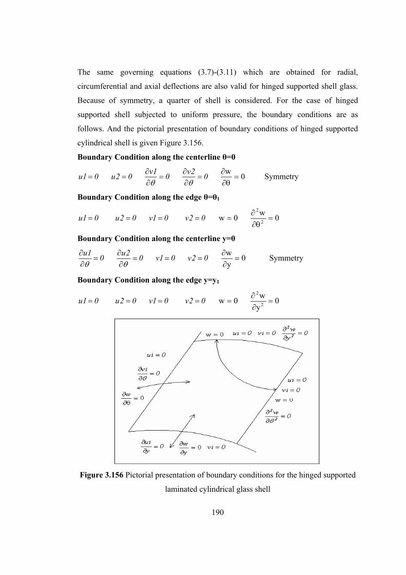
190
The same governing equations (3.7)-(3.11) which are obtained for radial,
circumferential and axial deflections are also valid for hinged supported shell glass.
Because of symmetry, a quarter of shell is considered. For the case of hinged
supported shell subjected to uniform pressure, the boundary conditions are as
follows. And the pictorial presentation of boundary conditions of hinged supported
cylindrical shell is given Figure 3.156.
Boundary Condition along the centerline θ=0
01u 02u 01v
02v
0w
Symmetry
Boundary Condition along the edge θ=θ1
01u 02u 01v 02v 0w 0w2
2
Boundary Condition along the centerline y=0
01u
02u
01v 02v 0y
w
Symmetry
Boundary Condition along the edge y=y1
01u 02u 01v 02v 0w 0y
w2
2
Figure 3.156 Pictorial presentation of boundary conditions for the hinged supported
laminated cylindrical glass shell
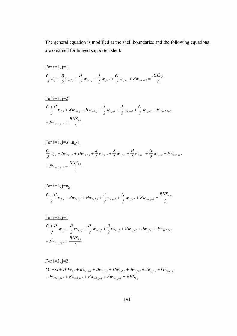
191
The general equation is modified at the shell boundaries and the following equations
are obtained for hinged supported shell:
For i=1, j=1
4
RHSFww
2
Gw
2
Jw
2
Hw
2
Bw
4
C i,j1,j1i2i,j1i,j,j2i,j1ii,j
For i=1, j=2
2
RHSFw
Fww2
Gw
2
Jw
2
JHwBww
2
GC
j,i1j,1i
1j,1i2j,i1j,i1j,ij,2ij,1ij,i
For i=1, j=3...ny-1
2
RHSFw
Fww2
Gw
2
Gw
2
Jw
2
JHwBww
2
C
j,i1j,1i
1j,1i2j,i2j,i1j,i1j,ij,2ij,1ij,i
For i=1, j=ny
2
RHSFww
2
Gw
2
JHwBww
2
GC j,i1j,1i2j,i1j,ij,2ij,1ij,i
For i=2, j=1
2
RHSFw
FwJwGww2
Bw
2
Hw
2
Bw
2
HC
j,i1j,1i
1j,1i1j,i2j,ij,1ij,2ij,1ij,i
For i=2, j=2
j,i1j,1i1j,1i1j,1i1j,1i
2j,i1j,i1j,ij,2ij,1ij,1ij,i
RHSFwFwFwFw
GwJwJwHwBwBww)HGC(
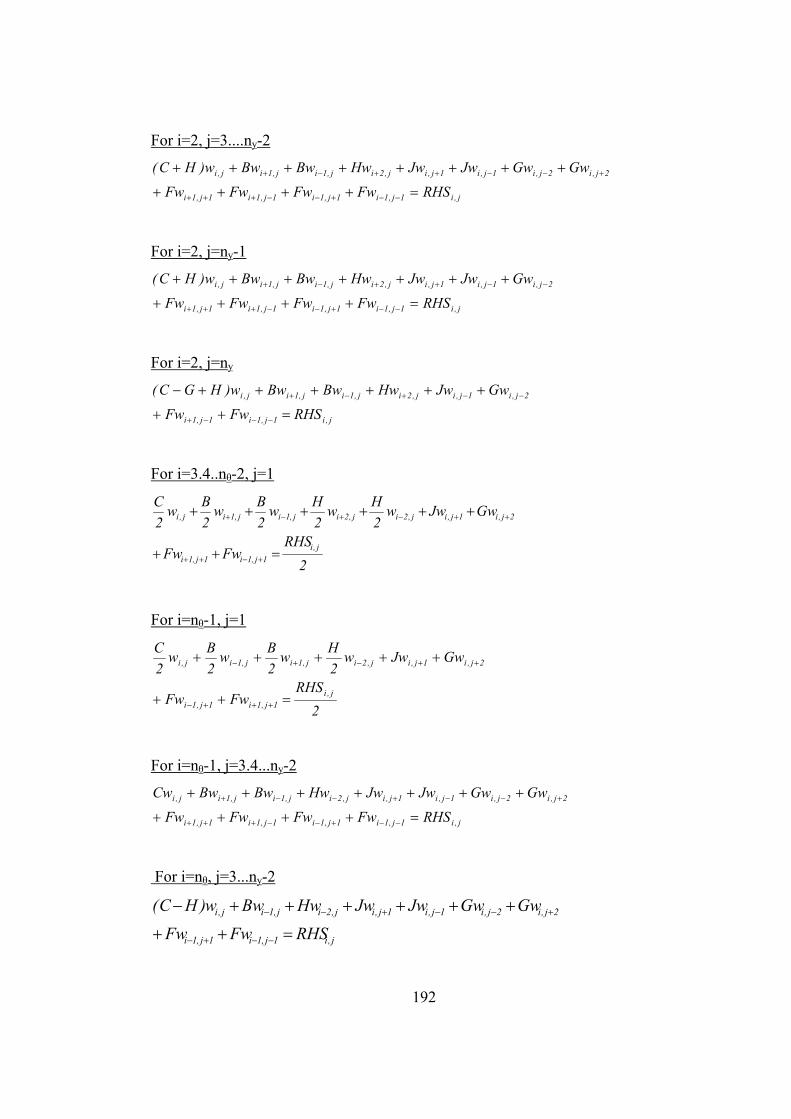
192
For i=2, j=3....ny-2
j,i1j,1i1j,1i1j,1i1j,1i
2j,i2j,i1j,i1j,ij,2ij,1ij,1ij,i
RHSFwFwFwFw
GwGwJwJwHwBwBww)HC(
For i=2, j=ny-1
j,i1j,1i1j,1i1j,1i1j,1i
2j,i1j,i1j,ij,2ij,1ij,1ij,i
RHSFwFwFwFw
GwJwJwHwBwBww)HC(
For i=2, j=ny
j,i1j,1i1j,1i
2j,i1j,ij,2ij,1ij,1ij,i
RHSFwFw
GwJwHwBwBww)HGC(
For i=3.4..nθ-2, j=1
2
RHSFwFw
GwJww2
Hw
2
Hw
2
Bw
2
Bw
2
C
j,i
1j,1i1j,1i
2j,i1j,ij,2ij,2ij,1ij,1ij,i
For i=nθ-1, j=1
2
RHSFwFw
GwJww2
Hw
2
Bw
2
Bw
2
C
j,i1j,1i1j,1i
2j,i1j,ij,2ij,1ij,1ij,i
For i=nθ-1, j=3.4...ny-2
j,i1j,1i1j,1i1j,1i1j,1i
2j,i2j,i1j,i1j,ij,2ij,1ij,1ij,i
RHSFwFwFwFw
GwGwJwJwHwBwBwCw
For i=nθ, j=3...ny-2
j,i1j,1i1j,1i
2j,i2j,i1j,i1j,ij,2ij,1ij,i
RHSFwFw
GwGwJwJwHwBww)HC(
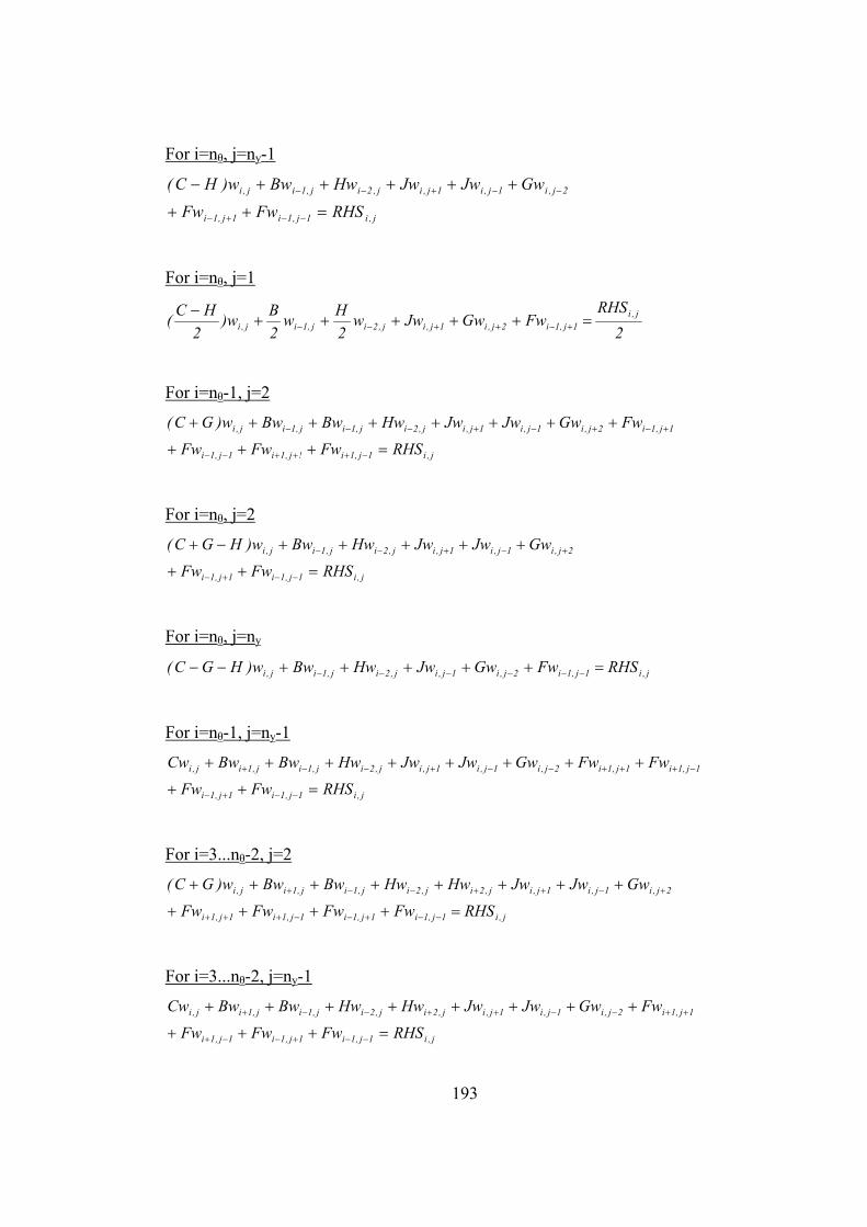
193
For i=nθ, j=ny-1
j,i1j,1i1j,1i
2j,i1j,i1j,ij,2ij,1ij,i
RHSFwFw
GwJwJwHwBww)HC(
For i=nθ, j=1
2
RHSFwGwJww
2
Hw
2
Bw)
2
HC( j,i
1j,1i2j,i1j,ij,2ij,1ij,i
For i=nθ-1, j=2
j,i1j,1i!j,1i1j,1i
1j,1i2j,i1j,i1j,ij,2ij,1ij,1ij,i
RHSFwFwFw
FwGwJwJwHwBwBww)GC(
For i=nθ, j=2
j,i1j,1i1j,1i
2j,i1j,i1j,ij,2ij,1ij,i
RHSFwFw
GwJwJwHwBww)HGC(
For i=nθ, j=ny
j,i1j,1i2j,i1j,ij,2ij,1ij,i RHSFwGwJwHwBww)HGC(
For i=nθ-1, j=ny-1
j,i1j,1i1j,1i
1j,1i1j,1i2j,i1j,i1j,ij,2ij,1ij,1ij,i
RHSFwFw
FwFwGwJwJwHwBwBwCw
For i=3...nθ-2, j=2
j,i1j,1i1j,1i1j,1i1j,1i
2j,i1j,i1j,ij,2ij,2ij,1ij,1ij,i
RHSFwFwFwFw
GwJwJwHwHwBwBww)GC(
For i=3...nθ-2, j=ny-1
j,i1j,1i1j,1i1j,1i
1j,1i2j,i1j,i1j,ij,2ij,2ij,1ij,1ij,i
RHSFwFwFw
FwGwJwJwHwHwBwBwCw
194
For i=3...nθ-2, j=ny
i,j1,j1i
1,j1i2i,j1i,j,j2i,j2i,j1i,j1ii,j
RHSFw
FwGwJwHwHwBwBwG)w(C
For i=nθ-1, j=ny
i,j1,j1i1,j1i2i,j1i,j,j2i,j1i,j1ii,j RHSFwFwGwJwHwBwBwG)w(C
The general equations for circumferential displacements (u1) are modified at the
shell boundaries and the following equations are obtained for hinged supported shell.
For i=2, j=1
j,ij,1ij,i1j,ij,ij,ij,ij,i1FU1u1AEU1u 1ASU1ANU1u1APU
For i=3.4…nθ-1, j=1
j,ij,1ij,i
j,1ij,i1j,ij,ij,ij,ij,i
1FU1u1AWU
1u1AEU1u 1ASU1ANU1u1APU
For i=nθ, j=1
j,ij,1ij,i1j,ij,ij,ij,ij,i1FU1u1AWU1u 1ASU1ANU1u1APU
For i=2, j=2.3.….ny-1
j,ij,1ij,i1j,ij,i1j,ij,ij,ij,i1FU1u1AEU1u1ASU1u1ANU1u1APU
For i=2, j=ny
j,ij,1ij,i1j,ij,ij,ij,i1FU1u1AEU1u1ASU1u1APU
For i=3.4.…nθ-1 , j=2.3.….ny-1
j,ij,1ij,i
j,1ij,i1j,ij,i1j,ij,ij,ij,i
1FU1u1AEU
1u1AWU1u1ASU1u1ANU1u1APU
195
For i=3.4.…nθ-1, j=ny
j,ij,1ij,ij,1ij,i1j,ij,ij,ij,i1FU1u1AEU1u1AWU1u1ASU1u1APU
For i=nθ, j=2.3.….ny-1
j,ij,1ij,i1j,ij,i1j,ij,ij,ij,i1FU1u1AWU1u1ASU1u1ANU1u1APU
For i=nθ, j=ny
j,ij,1ij,i1j,ij,ij,ij,i1FU1u1AWU1u1ASU1u1APU
The general equations for circumferential displacements (u2) are modified at the
shell boundaries and the following equations are obtained for hinged supported shell.
For i=2, j=1
j,ij,1ij,i1j,ij,ij,ij,ij,i2FU2u2AEU2u 2ASU2ANU2u2APU
For i=3.4.…nθ-1, j=1
j,ij,1ij,i
j,1ij,i1j,ij,ij,ij,ij,i
2FU2u2AWU
2u2AEU2u 2ASU2ANU2u2APU
For i=nθ, j=1
j,ij,1ij,i1j,ij,ij,ij,ij,i2FU2u2AWU2u 2ASU2ANU2u2APU
For i=2, j=2.3.….ny-1
j,ij,1ij,i1j,ij,i1j,ij,ij,ij,i2FU2u2AEU2u2ASU2u2ANU2u2APU
For i=2, j=ny
j,ij,1ij,i1j,ij,ij,ij,i2FU2u2AEU2u2ASU2u2APU
For i=3.4.…nθ-1 , j=2.3.….ny-1
j,ij,1ij,i
j,1ij,i1j,ij,i1j,ij,ij,ij,i
2FU2u2AEU
2u2AWU2u2ASU2u2ANU2u2APU
196
For i=3.4.…nθ-1, j=ny
j,ij,1ij,ij,1ij,i1j,ij,ij,ij,i2FU2u2AEU2u2AWU2u2ASU2u2APU
For i=nθ, j=2.3.….ny-1
j,ij,1ij,i1j,ij,i1j,ij,ij,ij,i2FU2u2AWU2u2ASU2u2ANU2u2APU
For i=nθ, j=ny
j,ij,1ij,i1j,ij,ij,ij,i2FU2u2AWU2u2ASU2u2APU
Modified axial displacements (v1) at the shell boundaries are obtained for hinged
supported shell as shown below:
For i=1, j=2
j,ij,1ij,ij,i1j,ij,ij,ij,i1FV1v 1AWV1AEV1v1ANV1v1APV
For i=2.3.…nθ-1, j=2
j,ij,1ij,ij,1ij,i1j,ij,ij,ij,i1FV1v1AEV1v1AWV1v1ANV1v1APV
For i=nθ, j=2
j,ij,1ij,i1j,ij,ij,ij,i1FV1v1AWV1v1ANV1v1APV
For i=1, j=3.4.….ny-1
j,i
j,1ij,ij,i1j,ij,i1j,ij,ij,ij,i
1FV
1v 1AWV1AEV1v1ANV1v1ASV1v1APV
For i=1, =ny
j,ij,1ij,ij,i1j,ij,ij,ij,i1FV1v 1AWV1AEV1v1ASV1v1APV
For i=2.3.…nθ-1, =3.4.….ny-1
j,ij,1ij,i
j,1ij,i1j,ij,i1j,ij,ij,ij,i
1FV1v1AEV
1v1AWV1v1ANV1v1ASV1v1APV
197
For i=2.3.…nθ-1, j=ny
j,ij,1ij,ij,1ij,i1j,ij,ij,ij,i1FV1v1AEV1v1AWV1v1ASV1v1APV
For i=nθ, j=3.4.….ny-1
j,ij,1ij,i1j,ij,i1j,ij,ij,ij,i1FV1v1AWV1v1ANV1v1ASV1v1APV
For i=nθ, j=ny
j,ij,1ij,i1j,ij,ij,ij,i1FV1v1AWV1v1ASV1v1APV
Modified axial displacements (v2) at the shell boundaries are obtained for hinged
supported shell as shown below:
For i=1, j=2
j,ij,1ij,ij,i1j,ij,ij,ij,i2FV2v 2AWV2AEV2v2ANV2v2APV
For i=2.3.…nθ-1, j=2
j,ij,1ij,ij,1ij,i1j,ij,ij,ij,i2FV2v2AEV2v2AWV2v2ANV2v2APV
For i=nθ, j=2
j,ij,1ij,i1j,ij,ij,ij,i2FV2v2AWV2v2ANV2v2APV
For i=1, j=3.4.….ny-1
j,i
j,1ij,ij,i1j,ij,i1j,ij,ij,ij,i
2FV
2v 2AWV2AEV2v2ANV2v2ASV2v2APV
For i=1, =ny
j,ij,1ij,ij,i1j,ij,ij,ij,i2FV2v 2AWV2AEV2v2ASV2v2APV
For i=2.3.…nθ-1, =3.4.….ny-1
j,ij,1ij,i
j,1ij,i1j,ij,i1j,ij,ij,ij,i
2FV2v2AEV
2v2AWV2v2ANV2v2ASV2v2APV
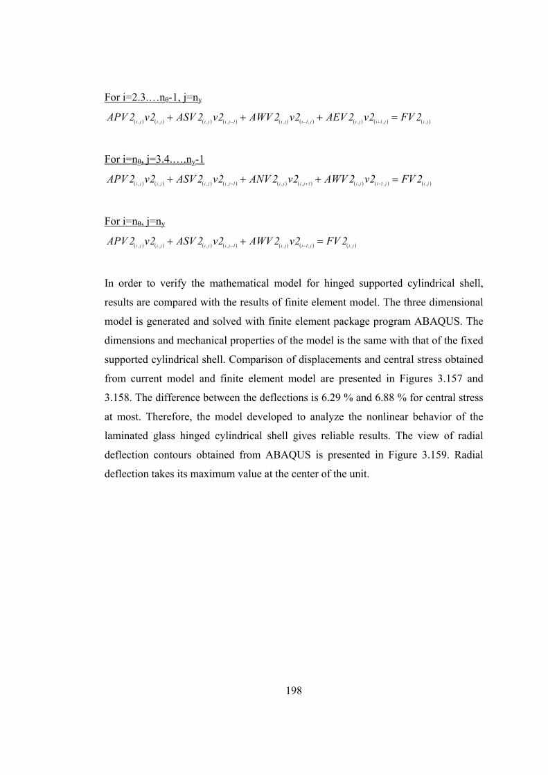
198
For i=2.3.…nθ-1, j=ny
j,ij,1ij,ij,1ij,i1j,ij,ij,ij,i2FV2v2AEV2v2AWV2v2ASV2v2APV
For i=nθ, j=3.4.….ny-1
j,ij,1ij,i1j,ij,i1j,ij,ij,ij,i2FV2v2AWV2v2ANV2v2ASV2v2APV
For i=nθ, j=ny
j,ij,1ij,i1j,ij,ij,ij,i2FV2v2AWV2v2ASV2v2APV
In order to verify the mathematical model for hinged supported cylindrical shell,
results are compared with the results of finite element model. The three dimensional
model is generated and solved with finite element package program ABAQUS. The
dimensions and mechanical properties of the model is the same with that of the fixed
supported cylindrical shell. Comparison of displacements and central stress obtained
from current model and finite element model are presented in Figures 3.157 and
3.158. The difference between the deflections is 6.29 % and 6.88 % for central stress
at most. Therefore, the model developed to analyze the nonlinear behavior of the
laminated glass hinged cylindrical shell gives reliable results. The view of radial
deflection contours obtained from ABAQUS is presented in Figure 3.159. Radial
deflection takes its maximum value at the center of the unit.
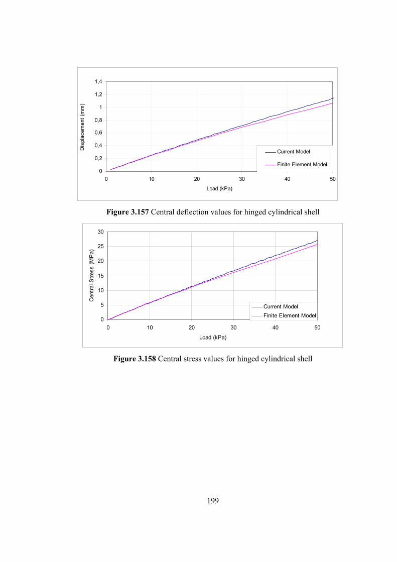
199
0
0,2
0,4
0,6
0,8
1
1,2
1,4
0 10 20 30 40 50
Load (kPa)
Dis
plac
emen
t (m
m)
Current Model
Finite Element Model
Figure 3.157 Central deflection values for hinged cylindrical shell
0
5
10
15
20
25
30
0 10 20 30 40 50
Load (kPa)
Cen
tral
Str
ess
(MP
a)
Current Model
Finite Element Model
Figure 3.158 Central stress values for hinged cylindrical shell
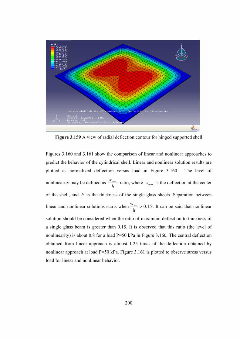
200
Figure 3.159 A view of radial deflection contour for hinged supported shell
Figures 3.160 and 3.161 show the comparison of linear and nonlinear approaches to
predict the behavior of the cylindrical shell. Linear and nonlinear solution results are
plotted as normalized deflection versus load in Figure 3.160. The level of
nonlinearity may be defined as h
wmax ratio, where maxw is the deflection at the center
of the shell, and h is the thickness of the single glass sheets. Separation between
linear and nonlinear solutions starts when 15.0h
wmax . It can be said that nonlinear
solution should be considered when the ratio of maximum deflection to thickness of
a single glass beam is greater than 0.15. It is observed that this ratio (the level of
nonlinearity) is about 0.8 for a load P=50 kPa in Figure 3.160. The central deflection
obtained from linear approach is almost 1.25 times of the deflection obtained by
nonlinear approach at load P=50 kPa. Figure 3.161 is plotted to observe stress versus
load for linear and nonlinear behavior.
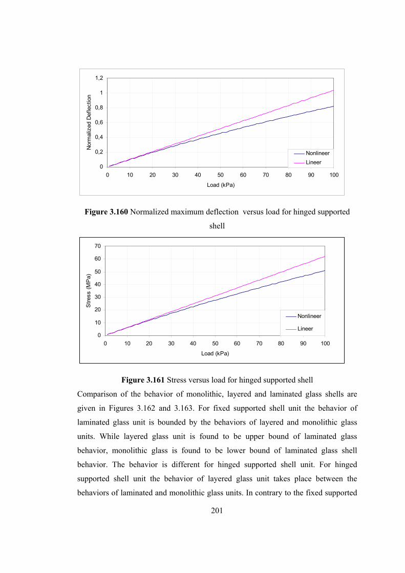
201
0
0,2
0,4
0,6
0,8
1
1,2
0 10 20 30 40 50 60 70 80 90 100
Load (kPa)
Nor
mal
ized
Def
lect
ion
Nonlineer
Lineer
Figure 3.160 Normalized maximum deflection versus load for hinged supported
shell
0
10
20
30
40
50
60
70
0 10 20 30 40 50 60 70 80 90 100
Load (kPa)
Str
ess
(MP
a)
Nonlineer
Lineer
Figure 3.161 Stress versus load for hinged supported shell
Comparison of the behavior of monolithic, layered and laminated glass shells are
given in Figures 3.162 and 3.163. For fixed supported shell unit the behavior of
laminated glass unit is bounded by the behaviors of layered and monolithic glass
units. While layered glass unit is found to be upper bound of laminated glass
behavior, monolithic glass is found to be lower bound of laminated glass shell
behavior. The behavior is different for hinged supported shell unit. For hinged
supported shell unit the behavior of layered glass unit takes place between the
behaviors of laminated and monolithic glass units. In contrary to the fixed supported
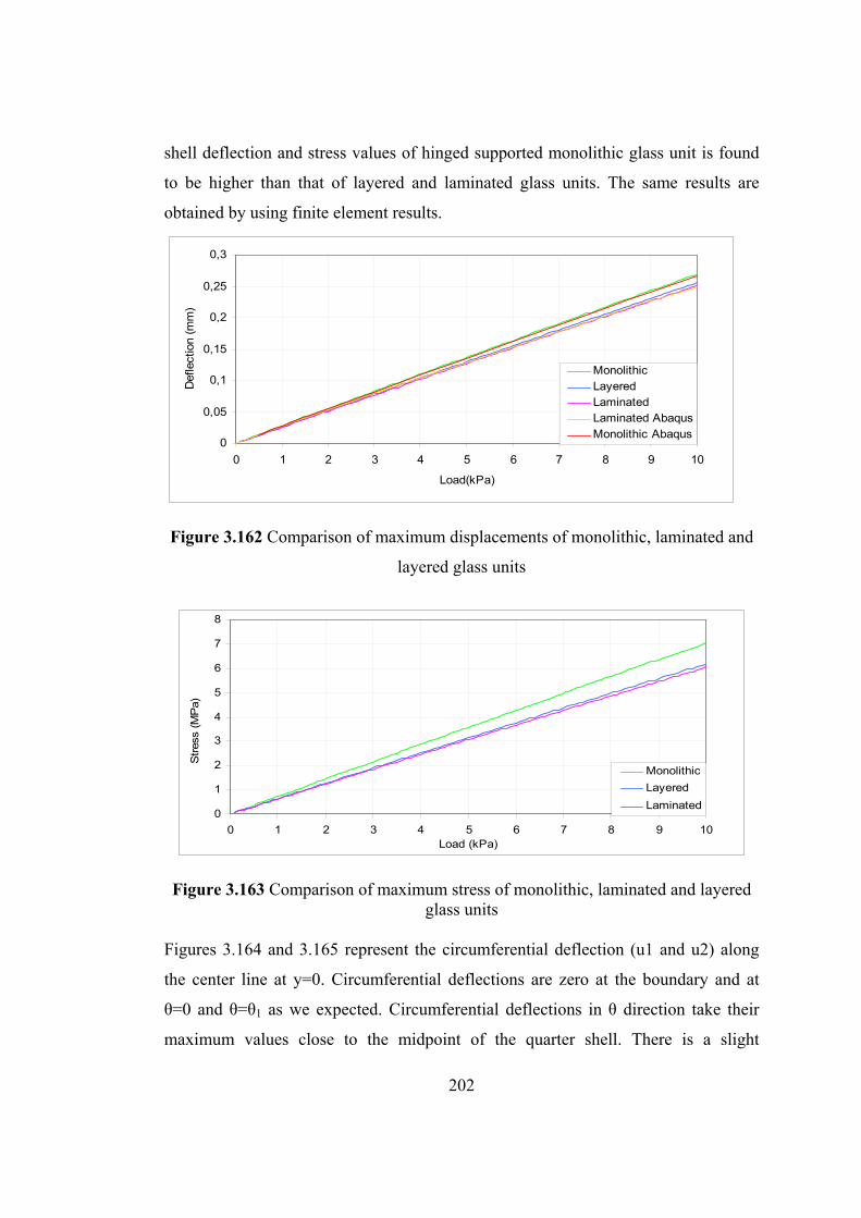
202
shell deflection and stress values of hinged supported monolithic glass unit is found
to be higher than that of layered and laminated glass units. The same results are
obtained by using finite element results.
0
0,05
0,1
0,15
0,2
0,25
0,3
0 1 2 3 4 5 6 7 8 9 10
Load(kPa)
Def
lect
ion
(mm
)
MonolithicLayeredLaminatedLaminated AbaqusMonolithic Abaqus
Figure 3.162 Comparison of maximum displacements of monolithic, laminated and
layered glass units
0
1
2
3
4
5
6
7
8
0 1 2 3 4 5 6 7 8 9 10Load (kPa)
Str
ess
(MP
a)
Monolithic
Layered
Laminated
Figure 3.163 Comparison of maximum stress of monolithic, laminated and layered glass units
Figures 3.164 and 3.165 represent the circumferential deflection (u1 and u2) along
the center line at y=0. Circumferential deflections are zero at the boundary and at
θ=0 and θ=θ1 as we expected. Circumferential deflections in θ direction take their
maximum values close to the midpoint of the quarter shell. There is a slight
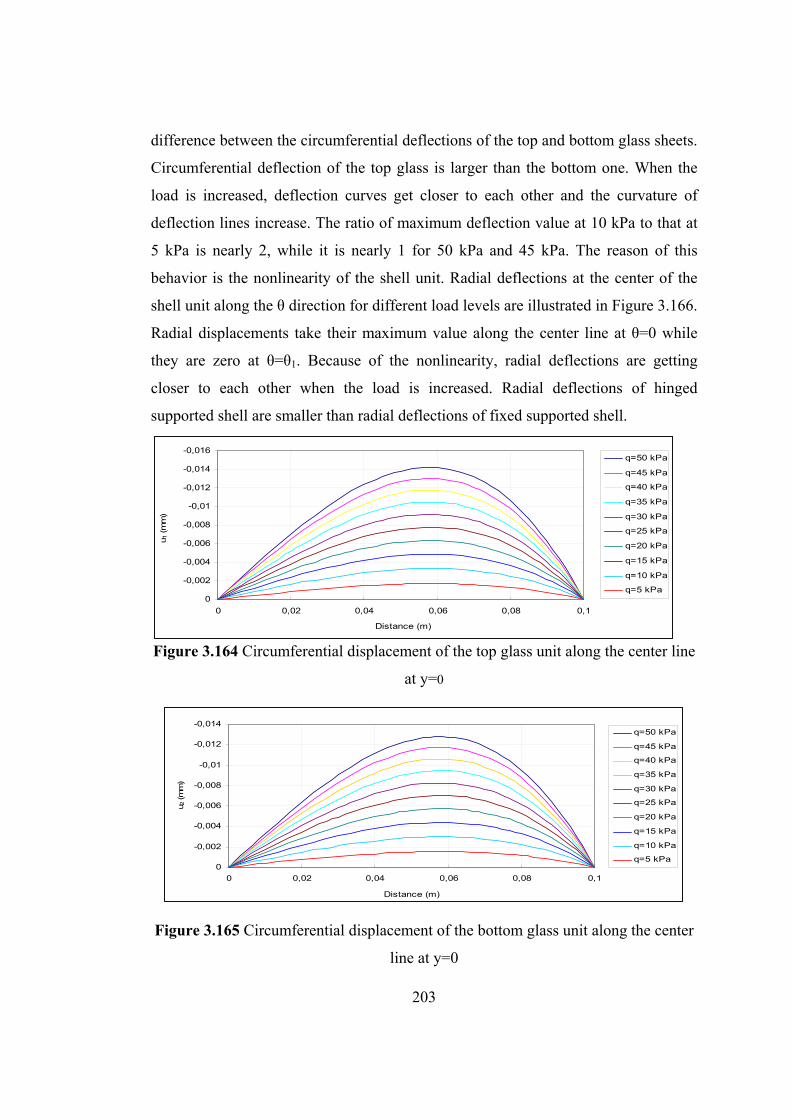
203
difference between the circumferential deflections of the top and bottom glass sheets.
Circumferential deflection of the top glass is larger than the bottom one. When the
load is increased, deflection curves get closer to each other and the curvature of
deflection lines increase. The ratio of maximum deflection value at 10 kPa to that at
5 kPa is nearly 2, while it is nearly 1 for 50 kPa and 45 kPa. The reason of this
behavior is the nonlinearity of the shell unit. Radial deflections at the center of the
shell unit along the θ direction for different load levels are illustrated in Figure 3.166.
Radial displacements take their maximum value along the center line at θ=0 while
they are zero at θ=θ1. Because of the nonlinearity, radial deflections are getting
closer to each other when the load is increased. Radial deflections of hinged
supported shell are smaller than radial deflections of fixed supported shell.
-0,016
-0,014
-0,012
-0,01
-0,008
-0,006
-0,004
-0,002
0
0 0,02 0,04 0,06 0,08 0,1
Distance (m)
u 1 (m
m)
q=50 kPa
q=45 kPa
q=40 kPa
q=35 kPa
q=30 kPa
q=25 kPa
q=20 kPa
q=15 kPa
q=10 kPa
q=5 kPa
Figure 3.164 Circumferential displacement of the top glass unit along the center line
at y=0
-0,014
-0,012
-0,01
-0,008
-0,006
-0,004
-0,002
0
0 0,02 0,04 0,06 0,08 0,1
Distance (m)
u 2 (m
m)
q=50 kPa
q=45 kPa
q=40 kPa
q=35 kPa
q=30 kPa
q=25 kPa
q=20 kPa
q=15 kPa
q=10 kPa
q=5 kPa
Figure 3.165 Circumferential displacement of the bottom glass unit along the center
line at y=0
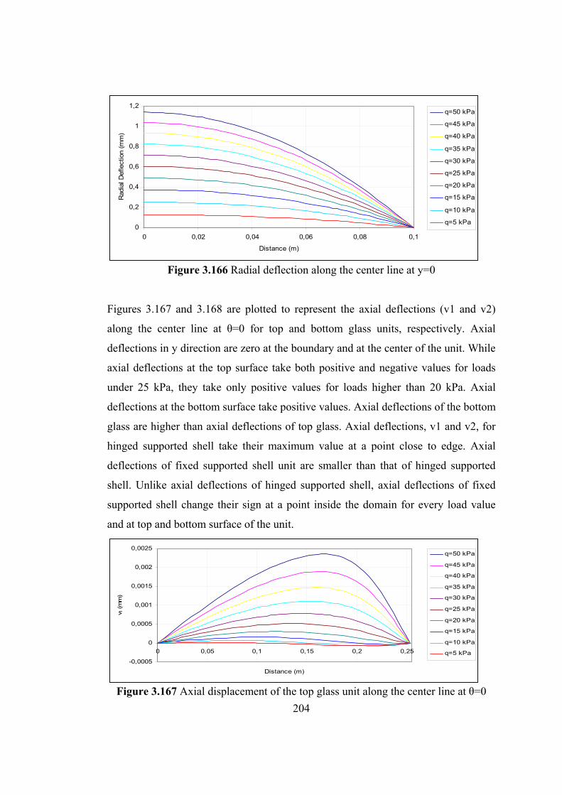
204
0
0,2
0,4
0,6
0,8
1
1,2
0 0,02 0,04 0,06 0,08 0,1
Distance (m)
Rad
ial D
efle
ctio
n (m
m)
q=50 kPa
q=45 kPa
q=40 kPa
q=35 kPa
q=30 kPa
q=25 kPa
q=20 kPa
q=15 kPa
q=10 kPa
q=5 kPa
Figure 3.166 Radial deflection along the center line at y=0
Figures 3.167 and 3.168 are plotted to represent the axial deflections (v1 and v2)
along the center line at θ=0 for top and bottom glass units, respectively. Axial
deflections in y direction are zero at the boundary and at the center of the unit. While
axial deflections at the top surface take both positive and negative values for loads
under 25 kPa, they take only positive values for loads higher than 20 kPa. Axial
deflections at the bottom surface take positive values. Axial deflections of the bottom
glass are higher than axial deflections of top glass. Axial deflections, v1 and v2, for
hinged supported shell take their maximum value at a point close to edge. Axial
deflections of fixed supported shell unit are smaller than that of hinged supported
shell. Unlike axial deflections of hinged supported shell, axial deflections of fixed
supported shell change their sign at a point inside the domain for every load value
and at top and bottom surface of the unit.
-0,0005
0
0,0005
0,001
0,0015
0,002
0,0025
0 0,05 0,1 0,15 0,2 0,25
Distance (m)
v 1 (m
m)
q=50 kPa
q=45 kPa
q=40 kPa
q=35 kPa
q=30 kPa
q=25 kPa
q=20 kPa
q=15 kPa
q=10 kPa
q=5 kPa
Figure 3.167 Axial displacement of the top glass unit along the center line at θ=0
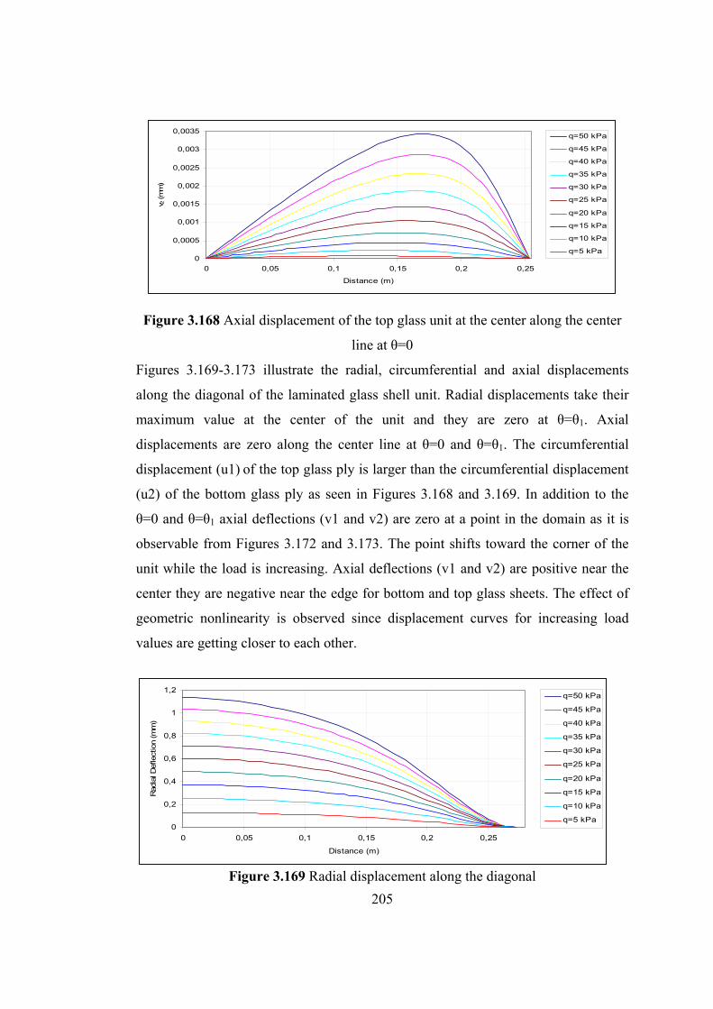
205
0
0,0005
0,001
0,0015
0,002
0,0025
0,003
0,0035
0 0,05 0,1 0,15 0,2 0,25
Distance (m)
v 2 (m
m)
q=50 kPa
q=45 kPa
q=40 kPa
q=35 kPa
q=30 kPa
q=25 kPa
q=20 kPa
q=15 kPa
q=10 kPa
q=5 kPa
Figure 3.168 Axial displacement of the top glass unit at the center along the center
line at θ=0
Figures 3.169-3.173 illustrate the radial, circumferential and axial displacements
along the diagonal of the laminated glass shell unit. Radial displacements take their
maximum value at the center of the unit and they are zero at θ=θ1. Axial
displacements are zero along the center line at θ=0 and θ=θ1. The circumferential
displacement (u1) of the top glass ply is larger than the circumferential displacement
(u2) of the bottom glass ply as seen in Figures 3.168 and 3.169. In addition to the
θ=0 and θ=θ1 axial deflections (v1 and v2) are zero at a point in the domain as it is
observable from Figures 3.172 and 3.173. The point shifts toward the corner of the
unit while the load is increasing. Axial deflections (v1 and v2) are positive near the
center they are negative near the edge for bottom and top glass sheets. The effect of
geometric nonlinearity is observed since displacement curves for increasing load
values are getting closer to each other.
0
0,2
0,4
0,6
0,8
1
1,2
0 0,05 0,1 0,15 0,2 0,25
Distance (m)
Rad
ial D
efle
ctio
n (m
m)
q=50 kPa
q=45 kPa
q=40 kPa
q=35 kPa
q=30 kPa
q=25 kPa
q=20 kPa
q=15 kPa
q=10 kPa
q=5 kPa
Figure 3.169 Radial displacement along the diagonal
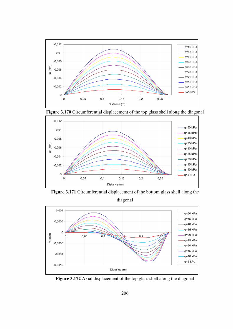
206
-0,012
-0,01
-0,008
-0,006
-0,004
-0,002
0
0 0,05 0,1 0,15 0,2 0,25
Distance (m)
u 1 (
mm
)q=50 kPa
q=45 kPa
q=40 kPa
q=35 kPa
q=30 kPa
q=25 kPa
q=20 kPa
q=15 kPa
q=10 kPa
q=5 kPa
Figure 3.170 Circumferential displacement of the top glass shell along the diagonal
-0,012
-0,01
-0,008
-0,006
-0,004
-0,002
0
0 0,05 0,1 0,15 0,2 0,25
Distance (m)
u2 (
mm
)
q=50 kPa
q=45 kPa
q=40 kPa
q=35 kPa
q=30 kPa
q=25 kPa
q=20 kPa
q=15 kPa
q=10 kPa
q=5 kPa
Figure 3.171 Circumferential displacement of the bottom glass shell along the
diagonal
-0,0015
-0,001
-0,0005
0
0,0005
0,001
0 0,05 0,1 0,15 0,2 0,25
Distance (m)
v 1 (
mm
)
q=50 kPa
q=45 kPa
q=40 kPa
q=35 kPa
q=30 kPa
q=25 kPa
q=20 kPa
q=15 kPa
q=10 kPa
q=5 kPa
Figure 3.172 Axial displacement of the top glass shell along the diagonal
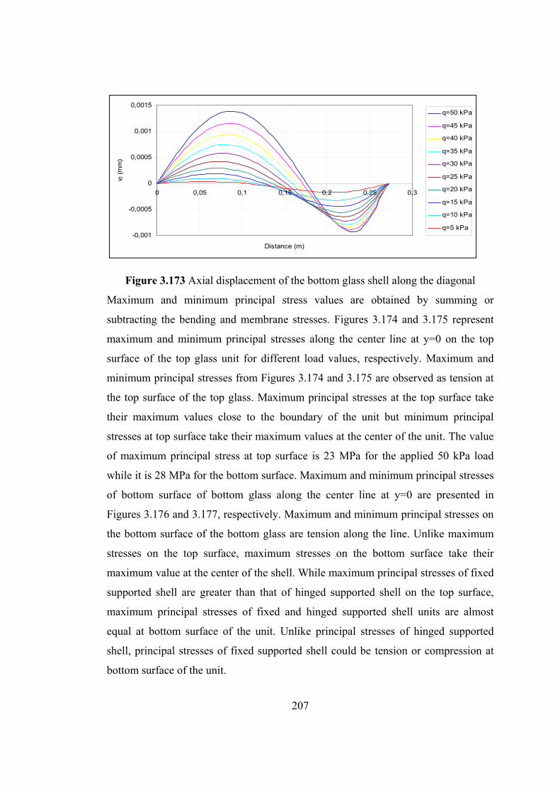
207
-0,001
-0,0005
0
0,0005
0,001
0,0015
0 0,05 0,1 0,15 0,2 0,25 0,3
Distance (m)
v 2 (
mm
)q=50 kPa
q=45 kPa
q=40 kPa
q=35 kPa
q=30 kPa
q=25 kPa
q=20 kPa
q=15 kPa
q=10 kPa
q=5 kPa
Figure 3.173 Axial displacement of the bottom glass shell along the diagonal
Maximum and minimum principal stress values are obtained by summing or
subtracting the bending and membrane stresses. Figures 3.174 and 3.175 represent
maximum and minimum principal stresses along the center line at y=0 on the top
surface of the top glass unit for different load values, respectively. Maximum and
minimum principal stresses from Figures 3.174 and 3.175 are observed as tension at
the top surface of the top glass. Maximum principal stresses at the top surface take
their maximum values close to the boundary of the unit but minimum principal
stresses at top surface take their maximum values at the center of the unit. The value
of maximum principal stress at top surface is 23 MPa for the applied 50 kPa load
while it is 28 MPa for the bottom surface. Maximum and minimum principal stresses
of bottom surface of bottom glass along the center line at y=0 are presented in
Figures 3.176 and 3.177, respectively. Maximum and minimum principal stresses on
the bottom surface of the bottom glass are tension along the line. Unlike maximum
stresses on the top surface, maximum stresses on the bottom surface take their
maximum value at the center of the shell. While maximum principal stresses of fixed
supported shell are greater than that of hinged supported shell on the top surface,
maximum principal stresses of fixed and hinged supported shell units are almost
equal at bottom surface of the unit. Unlike principal stresses of hinged supported
shell, principal stresses of fixed supported shell could be tension or compression at
bottom surface of the unit.
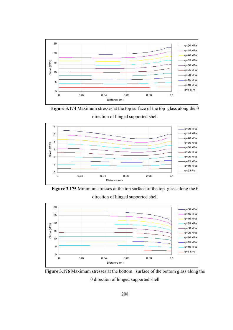
208
0
5
10
15
20
25
0 0,02 0,04 0,06 0,08 0,1
Distance (m)
Stres
s (M
Pa)
q=50 kPa
q=45 kPa
q=40 kPa
q=35 kPa
q=30 kPa
q=25 kPa
q=20 kPa
q=15 kPa
q=10 kPa
q=5 kPa
Figure 3.174 Maximum stresses at the top surface of the top glass along the θ
direction of hinged supported shell
0
1
2
3
4
5
6
0 0,02 0,04 0,06 0,08 0,1
Distance (m)
Stres
s (M
Pa)
q=50 kPa
q=45 kPa
q=40 kPa
q=35 kPa
q=30 kPa
q=25 kPa
q=20 kPa
q=15 kPa
q=10 kPa
q=5 kPa
Figure 3.175 Minimum stresses at the top surface of the top glass along the θ
direction of hinged supported shell
0
5
10
15
20
25
30
0 0,02 0,04 0,06 0,08 0,1
Distance (m)
Stres
s (M
Pa)
q=50 kPa
q=45 kPa
q=40 kPa
q=35 kPa
q=30 kPa
q=25 kPa
q=20 kPa
q=15 kPa
q=10 kPa
q=5 kPa
Figure 3.176 Maximum stresses at the bottom surface of the bottom glass along the
θ direction of hinged supported shell
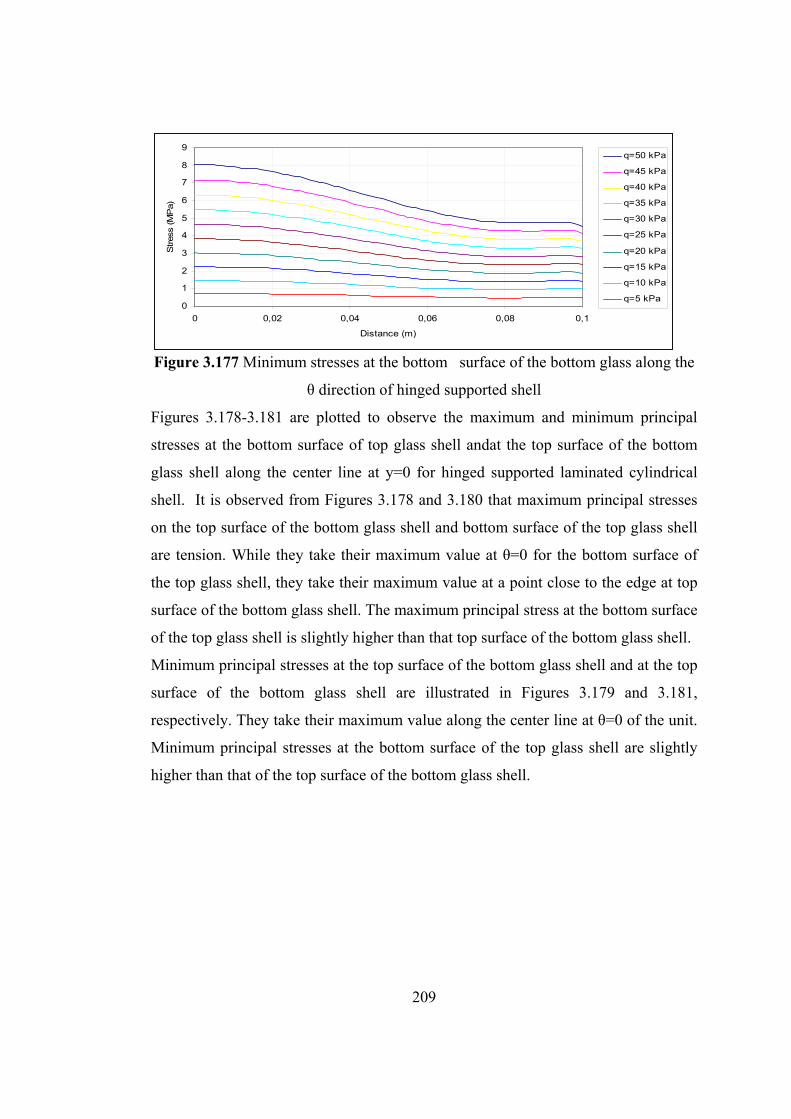
209
0
1
2
3
4
5
6
7
8
9
0 0,02 0,04 0,06 0,08 0,1
Distance (m)
Stres
s (M
Pa)
q=50 kPa
q=45 kPa
q=40 kPa
q=35 kPa
q=30 kPa
q=25 kPa
q=20 kPa
q=15 kPa
q=10 kPa
q=5 kPa
Figure 3.177 Minimum stresses at the bottom surface of the bottom glass along the
θ direction of hinged supported shell
Figures 3.178-3.181 are plotted to observe the maximum and minimum principal
stresses at the bottom surface of top glass shell andat the top surface of the bottom
glass shell along the center line at y=0 for hinged supported laminated cylindrical
shell. It is observed from Figures 3.178 and 3.180 that maximum principal stresses
on the top surface of the bottom glass shell and bottom surface of the top glass shell
are tension. While they take their maximum value at θ=0 for the bottom surface of
the top glass shell, they take their maximum value at a point close to the edge at top
surface of the bottom glass shell. The maximum principal stress at the bottom surface
of the top glass shell is slightly higher than that top surface of the bottom glass shell.
Minimum principal stresses at the top surface of the bottom glass shell and at the top
surface of the bottom glass shell are illustrated in Figures 3.179 and 3.181,
respectively. They take their maximum value along the center line at θ=0 of the unit.
Minimum principal stresses at the bottom surface of the top glass shell are slightly
higher than that of the top surface of the bottom glass shell.
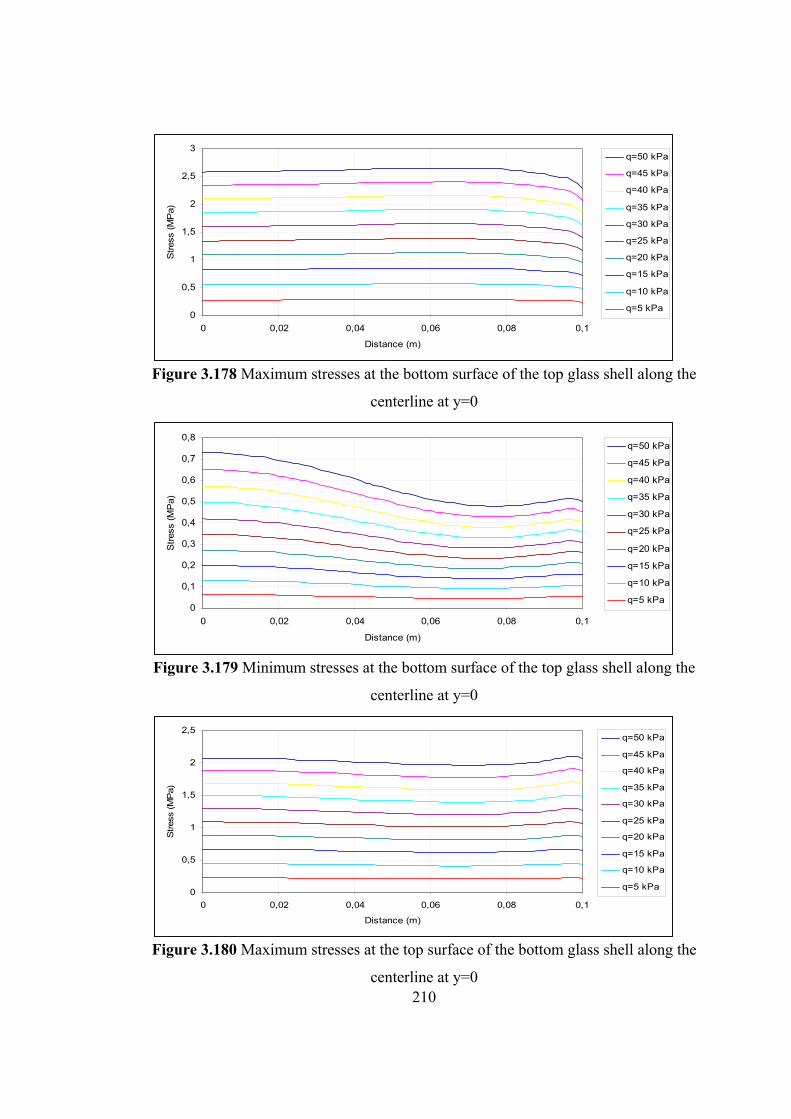
210
0
0,5
1
1,5
2
2,5
3
0 0,02 0,04 0,06 0,08 0,1
Distance (m)
Str
ess
(MP
a)
q=50 kPa
q=45 kPa
q=40 kPa
q=35 kPa
q=30 kPa
q=25 kPa
q=20 kPa
q=15 kPa
q=10 kPa
q=5 kPa
Figure 3.178 Maximum stresses at the bottom surface of the top glass shell along the
centerline at y=0
0
0,1
0,2
0,3
0,4
0,5
0,6
0,7
0,8
0 0,02 0,04 0,06 0,08 0,1
Distance (m)
Str
ess
(MP
a)
q=50 kPa
q=45 kPa
q=40 kPa
q=35 kPa
q=30 kPa
q=25 kPa
q=20 kPa
q=15 kPa
q=10 kPa
q=5 kPa
Figure 3.179 Minimum stresses at the bottom surface of the top glass shell along the
centerline at y=0
0
0,5
1
1,5
2
2,5
0 0,02 0,04 0,06 0,08 0,1
Distance (m)
Stres
s (M
Pa)
q=50 kPa
q=45 kPa
q=40 kPa
q=35 kPa
q=30 kPa
q=25 kPa
q=20 kPa
q=15 kPa
q=10 kPa
q=5 kPa
Figure 3.180 Maximum stresses at the top surface of the bottom glass shell along the
centerline at y=0
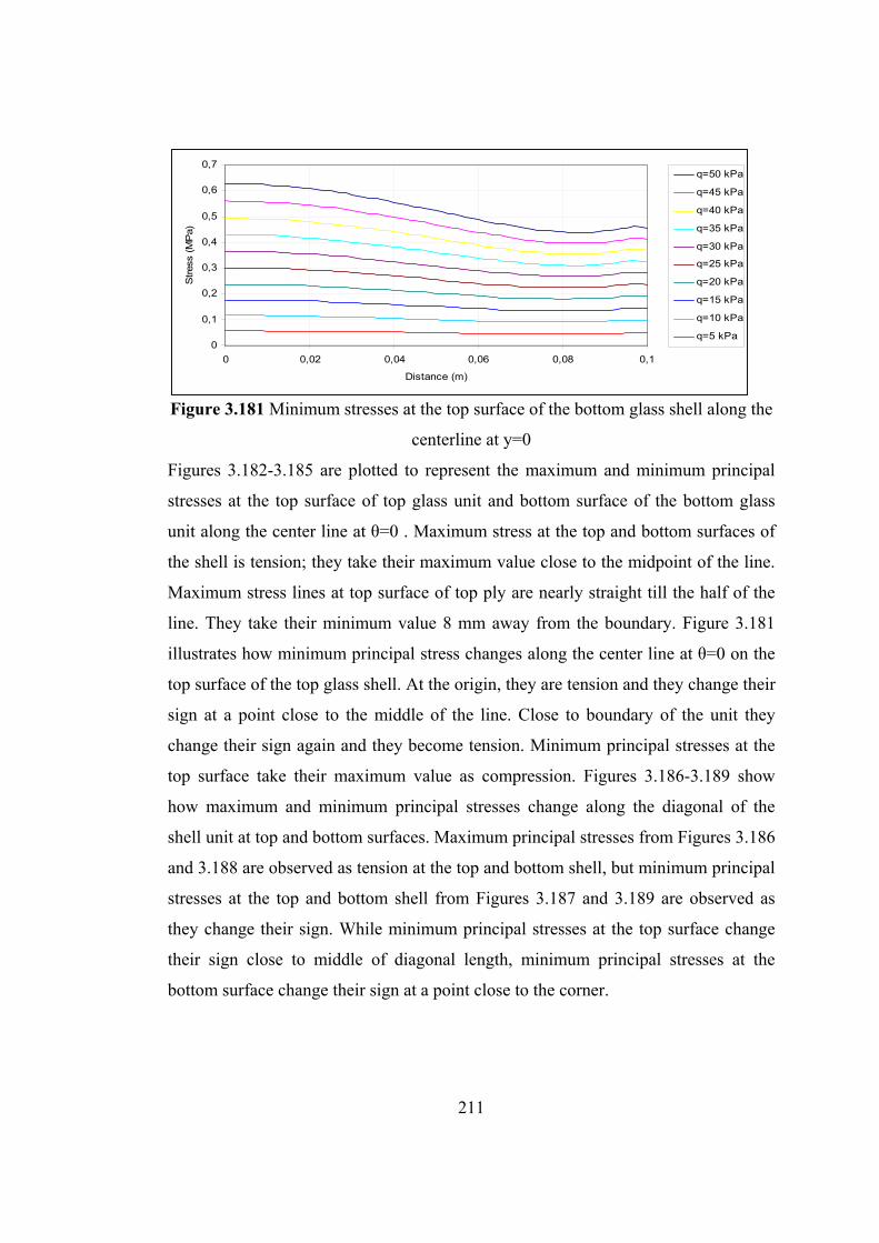
211
0
0,1
0,2
0,3
0,4
0,5
0,6
0,7
0 0,02 0,04 0,06 0,08 0,1
Distance (m)
Stres
s (M
Pa)
q=50 kPa
q=45 kPa
q=40 kPa
q=35 kPa
q=30 kPa
q=25 kPa
q=20 kPa
q=15 kPa
q=10 kPa
q=5 kPa
Figure 3.181 Minimum stresses at the top surface of the bottom glass shell along the
centerline at y=0
Figures 3.182-3.185 are plotted to represent the maximum and minimum principal
stresses at the top surface of top glass unit and bottom surface of the bottom glass
unit along the center line at θ=0 . Maximum stress at the top and bottom surfaces of
the shell is tension; they take their maximum value close to the midpoint of the line.
Maximum stress lines at top surface of top ply are nearly straight till the half of the
line. They take their minimum value 8 mm away from the boundary. Figure 3.181
illustrates how minimum principal stress changes along the center line at θ=0 on the
top surface of the top glass shell. At the origin, they are tension and they change their
sign at a point close to the middle of the line. Close to boundary of the unit they
change their sign again and they become tension. Minimum principal stresses at the
top surface take their maximum value as compression. Figures 3.186-3.189 show
how maximum and minimum principal stresses change along the diagonal of the
shell unit at top and bottom surfaces. Maximum principal stresses from Figures 3.186
and 3.188 are observed as tension at the top and bottom shell, but minimum principal
stresses at the top and bottom shell from Figures 3.187 and 3.189 are observed as
they change their sign. While minimum principal stresses at the top surface change
their sign close to middle of diagonal length, minimum principal stresses at the
bottom surface change their sign at a point close to the corner.
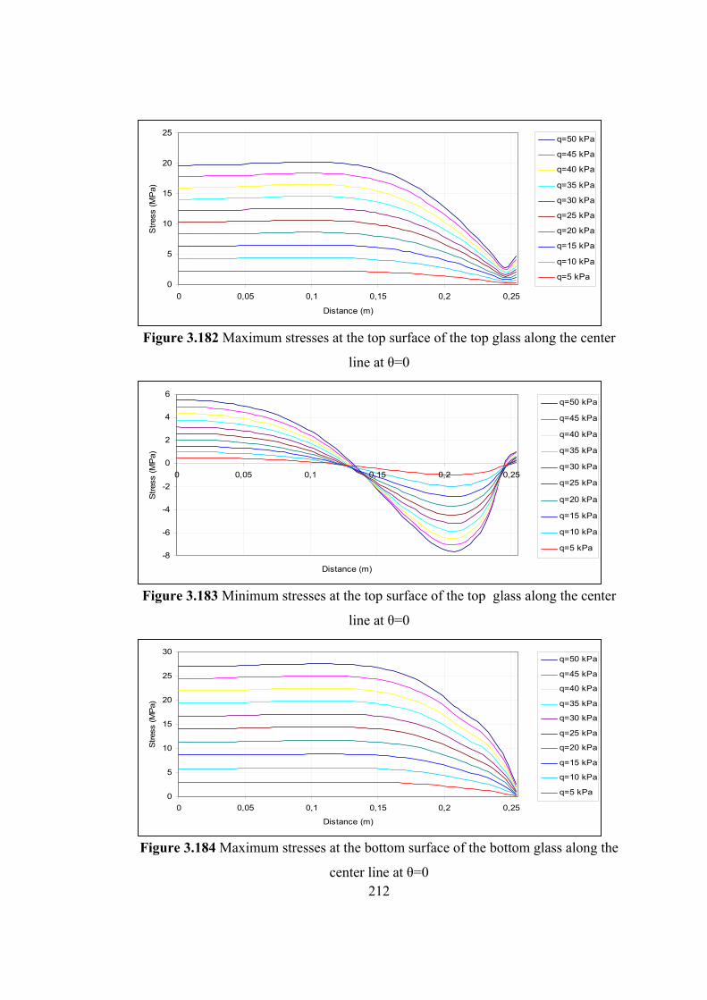
212
0
5
10
15
20
25
0 0,05 0,1 0,15 0,2 0,25
Distance (m)
Str
ess
(MP
a)
q=50 kPa
q=45 kPa
q=40 kPa
q=35 kPa
q=30 kPa
q=25 kPa
q=20 kPa
q=15 kPa
q=10 kPa
q=5 kPa
Figure 3.182 Maximum stresses at the top surface of the top glass along the center
line at θ=0
-8
-6
-4
-2
0
2
4
6
0 0,05 0,1 0,15 0,2 0,25
Distance (m)
Str
ess
(MP
a)
q=50 kPa
q=45 kPa
q=40 kPa
q=35 kPa
q=30 kPa
q=25 kPa
q=20 kPa
q=15 kPa
q=10 kPa
q=5 kPa
Figure 3.183 Minimum stresses at the top surface of the top glass along the center
line at θ=0
0
5
10
15
20
25
30
0 0,05 0,1 0,15 0,2 0,25
Distance (m)
Stres
s (M
Pa)
q=50 kPa
q=45 kPa
q=40 kPa
q=35 kPa
q=30 kPa
q=25 kPa
q=20 kPa
q=15 kPa
q=10 kPa
q=5 kPa
Figure 3.184 Maximum stresses at the bottom surface of the bottom glass along the
center line at θ=0
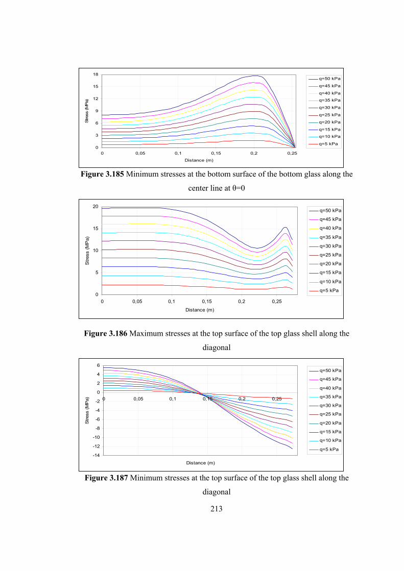
213
0
3
6
9
12
15
18
0 0,05 0,1 0,15 0,2 0,25
Distance (m)
Stres
s (M
Pa)
q=50 kPa
q=45 kPa
q=40 kPa
q=35 kPa
q=30 kPa
q=25 kPa
q=20 kPa
q=15 kPa
q=10 kPa
q=5 kPa
Figure 3.185 Minimum stresses at the bottom surface of the bottom glass along the
center line at θ=0
0
5
10
15
20
0 0,05 0,1 0,15 0,2 0,25
Distance (m)
Str
ess
(MP
a)
q=50 kPa
q=45 kPa
q=40 kPa
q=35 kPa
q=30 kPa
q=25 kPa
q=20 kPa
q=15 kPa
q=10 kPa
q=5 kPa
Figure 3.186 Maximum stresses at the top surface of the top glass shell along the
diagonal
-14
-12
-10
-8
-6
-4
-2
0
2
4
6
0 0,05 0,1 0,15 0,2 0,25
Distance (m)
Stres
s (M
Pa)
q=50 kPa
q=45 kPa
q=40 kPa
q=35 kPa
q=30 kPa
q=25 kPa
q=20 kPa
q=15 kPa
q=10 kPa
q=5 kPa
Figure 3.187 Minimum stresses at the top surface of the top glass shell along the
diagonal
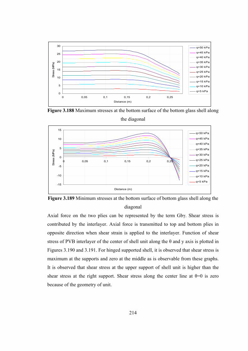
214
0
5
10
15
20
25
30
0 0,05 0,1 0,15 0,2 0,25
Distance (m)
Stres
s (M
Pa)
q=50 kPa
q=45 kPa
q=40 kPa
q=35 kPa
q=30 kPa
q=25 kPa
q=20 kPa
q=15 kPa
q=10 kPa
q=5 kPa
Figure 3.188 Maximum stresses at the bottom surface of the bottom glass shell along
the diagonal
-15
-10
-5
0
5
10
15
0 0,05 0,1 0,15 0,2 0,25
Distance (m)
Stres
s (M
Pa)
q=50 kPa
q=45 kPa
q=40 kPa
q=35 kPa
q=30 kPa
q=25 kPa
q=20 kPa
q=15 kPa
q=10 kPa
q=5 kPa
Figure 3.189 Minimum stresses at the bottom surface of bottom glass shell along the
diagonal
Axial force on the two plies can be represented by the term Gbγ. Shear stress is
contributed by the interlayer. Axial force is transmitted to top and bottom plies in
opposite direction when shear strain is applied to the interlayer. Function of shear
stress of PVB interlayer of the center of shell unit along the θ and y axis is plotted in
Figures 3.190 and 3.191. For hinged supported shell, it is observed that shear stress is
maximum at the supports and zero at the middle as is observable from these graphs.
It is observed that shear stress at the upper support of shell unit is higher than the
shear stress at the right support. Shear stress along the center line at θ=0 is zero
because of the geometry of unit.
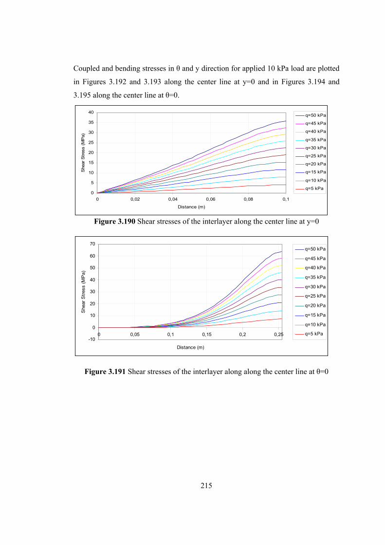
215
Coupled and bending stresses in θ and y direction for applied 10 kPa load are plotted
in Figures 3.192 and 3.193 along the center line at y=0 and in Figures 3.194 and
3.195 along the center line at θ=0.
0
5
10
15
20
25
30
35
40
0 0,02 0,04 0,06 0,08 0,1
Distance (m)
She
ar S
tres
s (M
Pa)
q=50 kPa
q=45 kPa
q=40 kPa
q=35 kPa
q=30 kPa
q=25 kPa
q=20 kPa
q=15 kPa
q=10 kPa
q=5 kPa
Figure 3.190 Shear stresses of the interlayer along the center line at y=0
-10
0
10
20
30
40
50
60
70
0 0,05 0,1 0,15 0,2 0,25
Distance (m)
She
ar S
tres
s (M
Pa)
q=50 kPa
q=45 kPa
q=40 kPa
q=35 kPa
q=30 kPa
q=25 kPa
q=20 kPa
q=15 kPa
q=10 kPa
q=5 kPa
Figure 3.191 Shear stresses of the interlayer along along the center line at θ=0
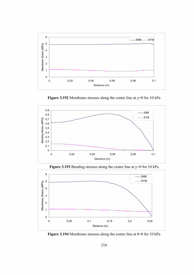
216
0
1
2
3
4
5
6
0 0,02 0,04 0,06 0,08 0,1
Distance (m)
Mem
bran
e S
tres
s (M
Pa)
SθM SYM
Figure 3.192 Membrane stresses along the center line at y=0 for 10 kPa
0
0,1
0,2
0,3
0,4
0,5
0,6
0,7
0,8
0,9
0 0,02 0,04 0,06 0,08 0,1
Distance (m)
Ben
ding
Str
ess
(MP
a)
SθB
SYB
Figure 3.193 Bending stresses along the center line at y=0 for 10 kPa
0
1
2
3
4
5
6
0 0,05 0,1 0,15 0,2 0,25
Distance (m)
Mem
bran
e S
tres
s (M
Pa)
SθM
SYM
Figure 3.194 Membrane stresses along the center line at θ=0 for 10 kPa
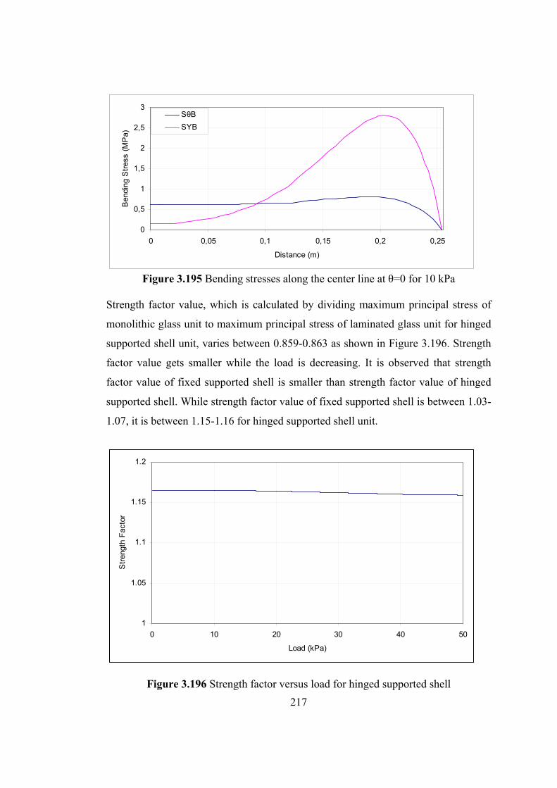
217
0
0,5
1
1,5
2
2,5
3
0 0,05 0,1 0,15 0,2 0,25
Distance (m)
Ben
ding
Str
ess
(MP
a)SθB
SYB
Figure 3.195 Bending stresses along the center line at θ=0 for 10 kPa
Strength factor value, which is calculated by dividing maximum principal stress of
monolithic glass unit to maximum principal stress of laminated glass unit for hinged
supported shell unit, varies between 0.859-0.863 as shown in Figure 3.196. Strength
factor value gets smaller while the load is decreasing. It is observed that strength
factor value of fixed supported shell is smaller than strength factor value of hinged
supported shell. While strength factor value of fixed supported shell is between 1.03-
1.07, it is between 1.15-1.16 for hinged supported shell unit.
1
1.05
1.1
1.15
1.2
0 10 20 30 40 50
Load (kPa)
Str
engt
h F
acto
r
Figure 3.196 Strength factor versus load for hinged supported shell
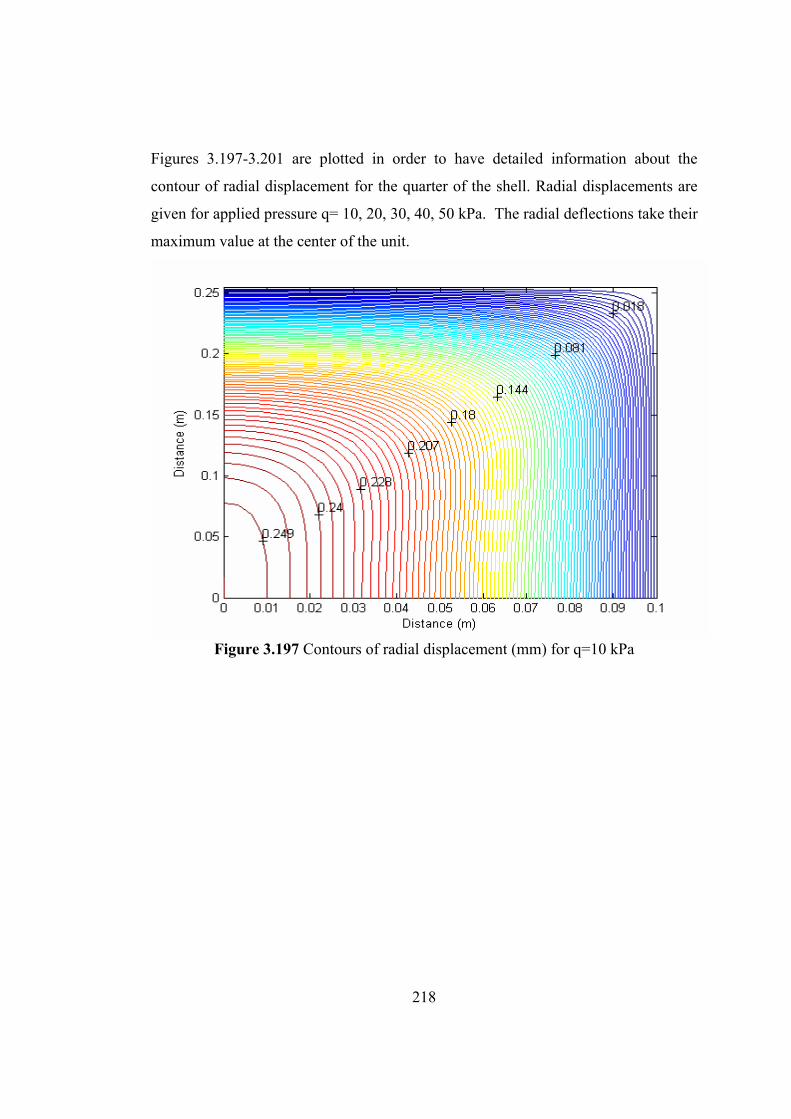
218
Figures 3.197-3.201 are plotted in order to have detailed information about the
contour of radial displacement for the quarter of the shell. Radial displacements are
given for applied pressure q= 10, 20, 30, 40, 50 kPa. The radial deflections take their
maximum value at the center of the unit.
Figure 3.197 Contours of radial displacement (mm) for q=10 kPa
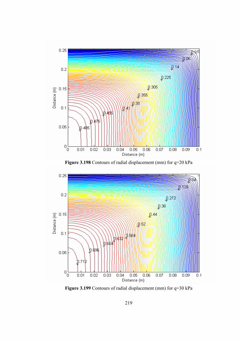
219
Figure 3.198 Contours of radial displacement (mm) for q=20 kPa
Figure 3.199 Contours of radial displacement (mm) for q=30 kPa
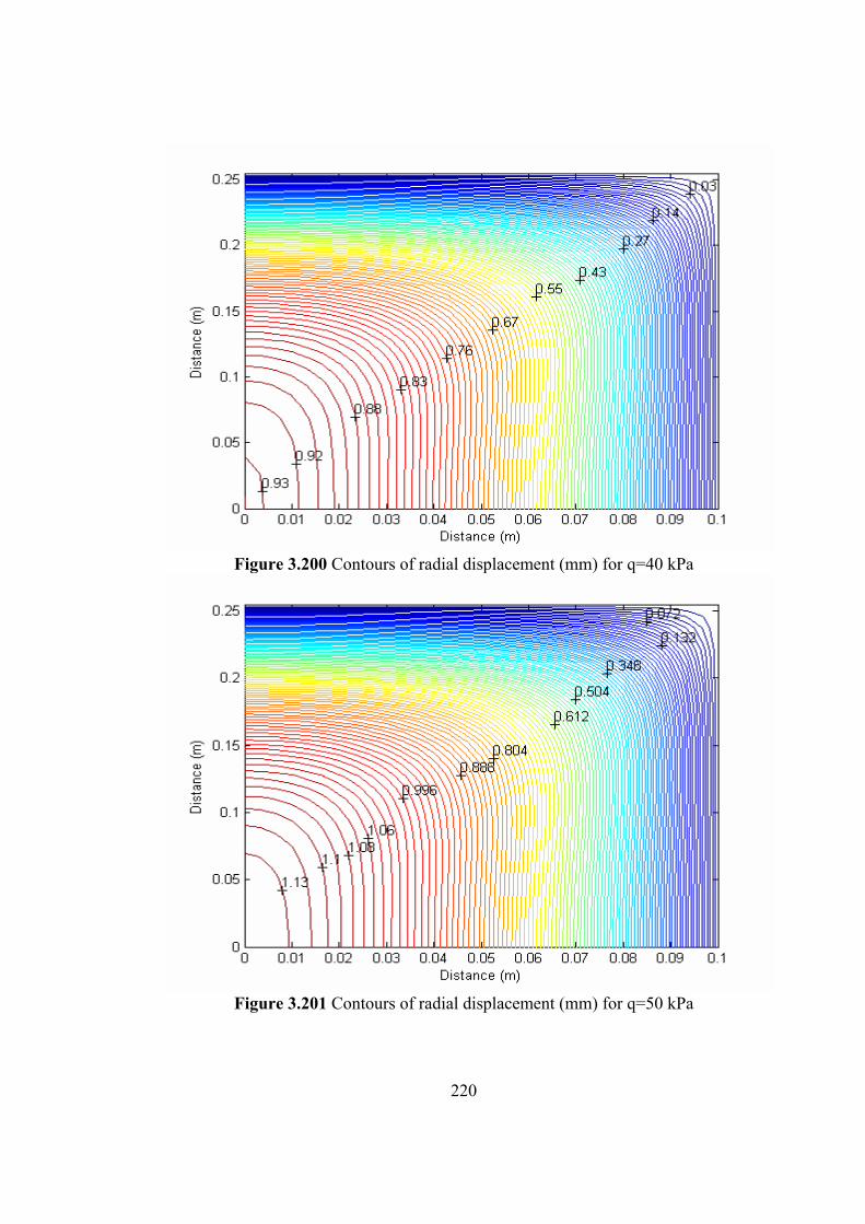
220
Figure 3.200 Contours of radial displacement (mm) for q=40 kPa
Figure 3.201 Contours of radial displacement (mm) for q=50 kPa
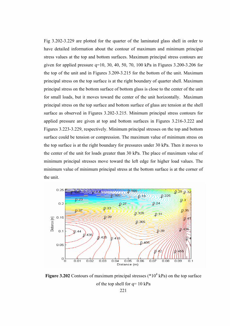
221
Fig 3.202-3.229 are plotted for the quarter of the laminated glass shell in order to
have detailed information about the contour of maximum and minimum principal
stress values at the top and bottom surfaces. Maximum principal stress contours are
given for applied pressure q=10, 30, 40, 50, 70, 100 kPa in Figures 3.200-3.206 for
the top of the unit and in Figures 3.209-3.215 for the bottom of the unit. Maximum
principal stress on the top surface is at the right boundary of quarter shell. Maximum
principal stress on the bottom surface of bottom glass is close to the center of the unit
for small loads, but it moves toward the center of the unit horizontally. Maximum
principal stress on the top surface and bottom surface of glass are tension at the shell
surface as observed in Figures 3.202-3.215. Minimum principal stress contours for
applied pressure are given at top and bottom surfaces in Figures 3.216-3.222 and
Figures 3.223-3.229, respectively. Minimum principal stresses on the top and bottom
surface could be tension or compression. The maximum value of minimum stress on
the top surface is at the right boundary for pressures under 30 kPa. Then it moves to
the center of the unit for loads greater than 30 kPa. The place of maximum value of
minimum principal stresses move toward the left edge for higher load values. The
minimum value of minimum principal stress at the bottom surface is at the corner of
the unit.
Figure 3.202 Contours of maximum principal stresses (*104 kPa) on the top surface
of the top shell for q= 10 kPa
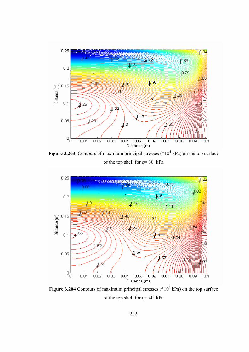
222
Figure 3.203 Contours of maximum principal stresses (*104 kPa) on the top surface
of the top shell for q= 30 kPa
Figure 3.204 Contours of maximum principal stresses (*104 kPa) on the top surface
of the top shell for q= 40 kPa
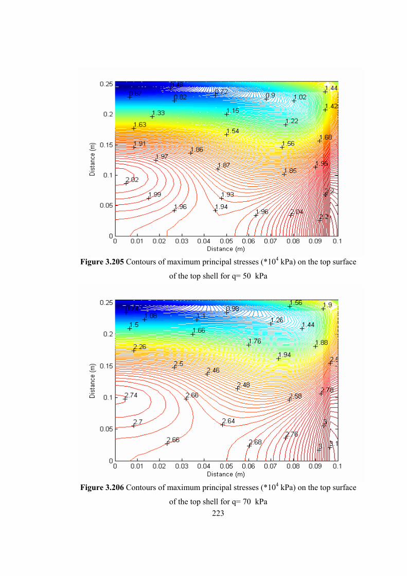
223
Figure 3.205 Contours of maximum principal stresses (*104 kPa) on the top surface
of the top shell for q= 50 kPa
Figure 3.206 Contours of maximum principal stresses (*104 kPa) on the top surface
of the top shell for q= 70 kPa
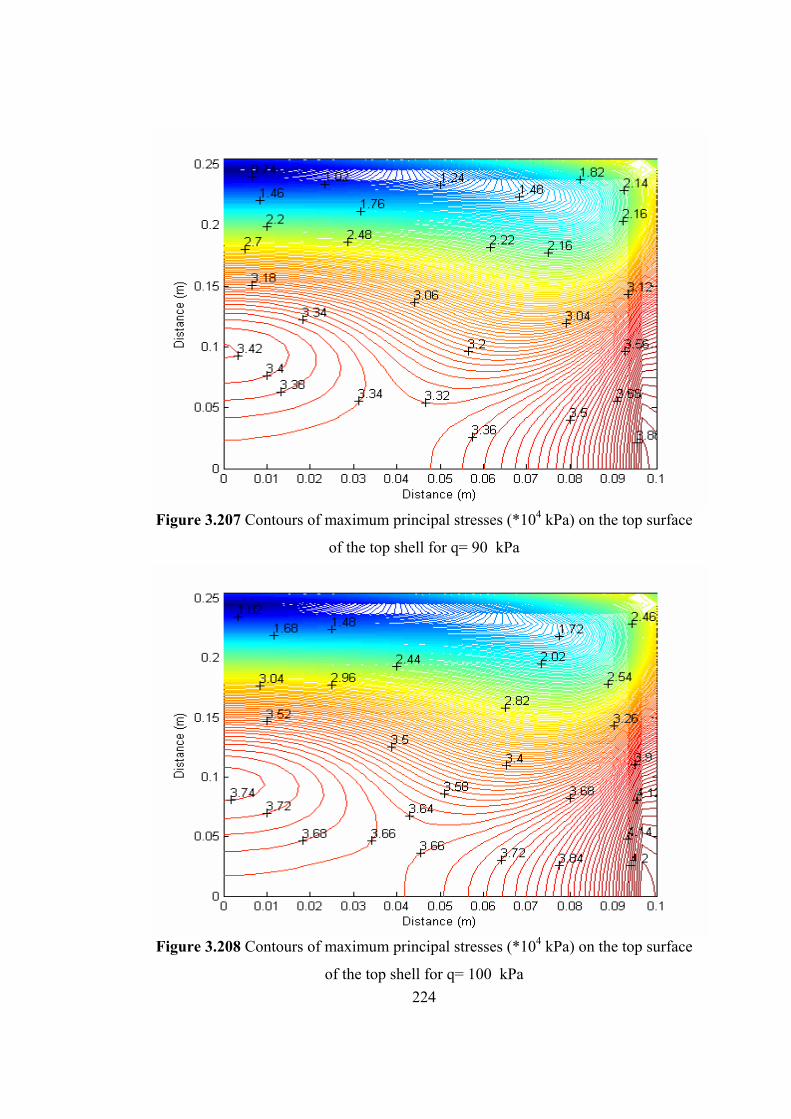
224
Figure 3.207 Contours of maximum principal stresses (*104 kPa) on the top surface
of the top shell for q= 90 kPa
Figure 3.208 Contours of maximum principal stresses (*104 kPa) on the top surface
of the top shell for q= 100 kPa
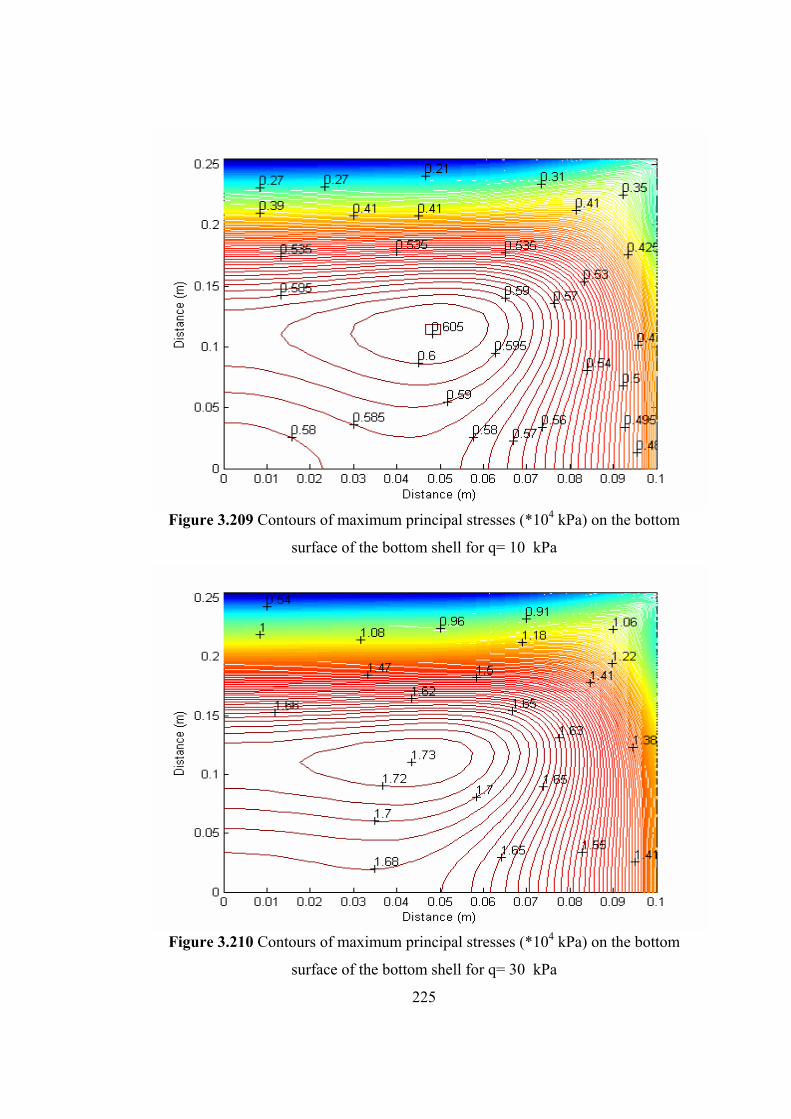
225
Figure 3.209 Contours of maximum principal stresses (*104 kPa) on the bottom
surface of the bottom shell for q= 10 kPa
Figure 3.210 Contours of maximum principal stresses (*104 kPa) on the bottom
surface of the bottom shell for q= 30 kPa
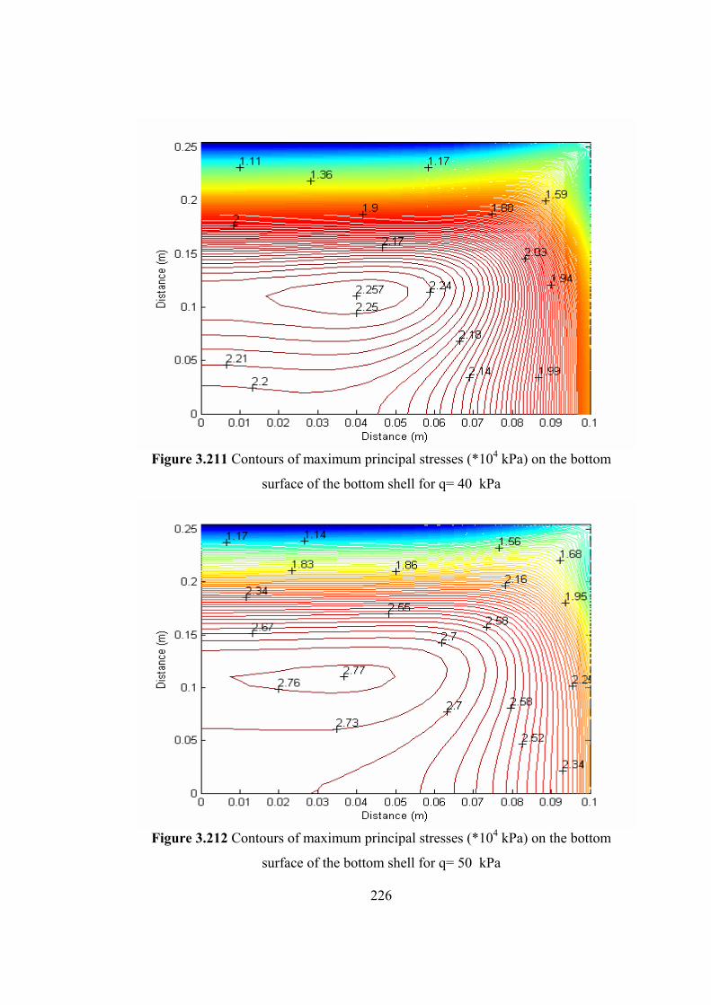
226
Figure 3.211 Contours of maximum principal stresses (*104 kPa) on the bottom
surface of the bottom shell for q= 40 kPa
Figure 3.212 Contours of maximum principal stresses (*104 kPa) on the bottom
surface of the bottom shell for q= 50 kPa
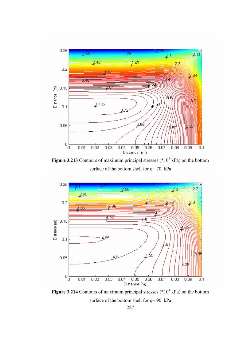
227
Figure 3.213 Contours of maximum principal stresses (*104 kPa) on the bottom
surface of the bottom shell for q= 70 kPa
Figure 3.214 Contours of maximum principal stresses (*104 kPa) on the bottom
surface of the bottom shell for q= 90 kPa
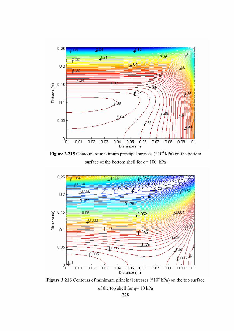
228
Figure 3.215 Contours of maximum principal stresses (*104 kPa) on the bottom
surface of the bottom shell for q= 100 kPa
Figure 3.216 Contours of minimum principal stresses (*104 kPa) on the top surface
of the top shell for q= 10 kPa
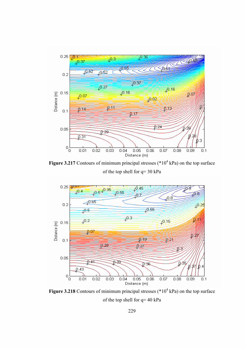
229
Figure 3.217 Contours of minimum principal stresses (*104 kPa) on the top surface
of the top shell for q= 30 kPa
Figure 3.218 Contours of minimum principal stresses (*104 kPa) on the top surface
of the top shell for q= 40 kPa
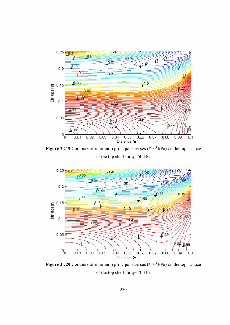
230
Figure 3.219 Contours of minimum principal stresses (*104 kPa) on the top surface
of the top shell for q= 50 kPa
Figure 3.220 Contours of minimum principal stresses (*104 kPa) on the top surface
of the top shell for q= 70 kPa
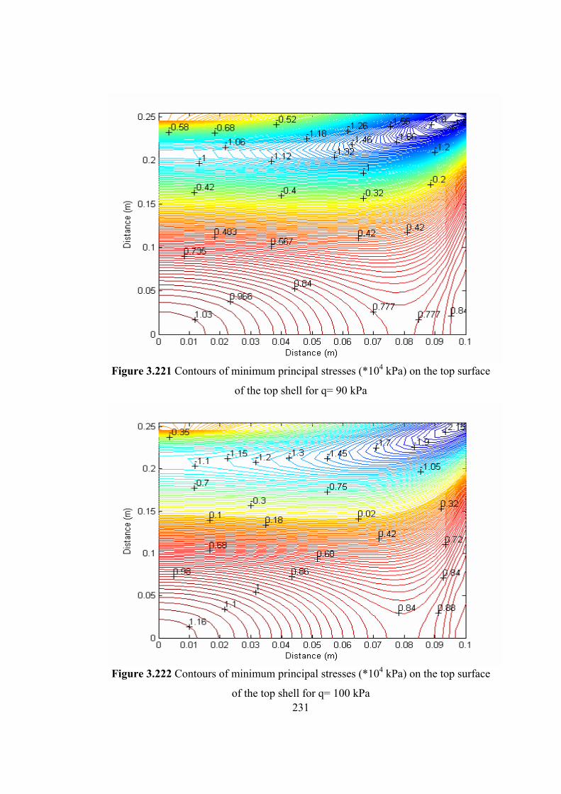
231
Figure 3.221 Contours of minimum principal stresses (*104 kPa) on the top surface
of the top shell for q= 90 kPa
Figure 3.222 Contours of minimum principal stresses (*104 kPa) on the top surface
of the top shell for q= 100 kPa
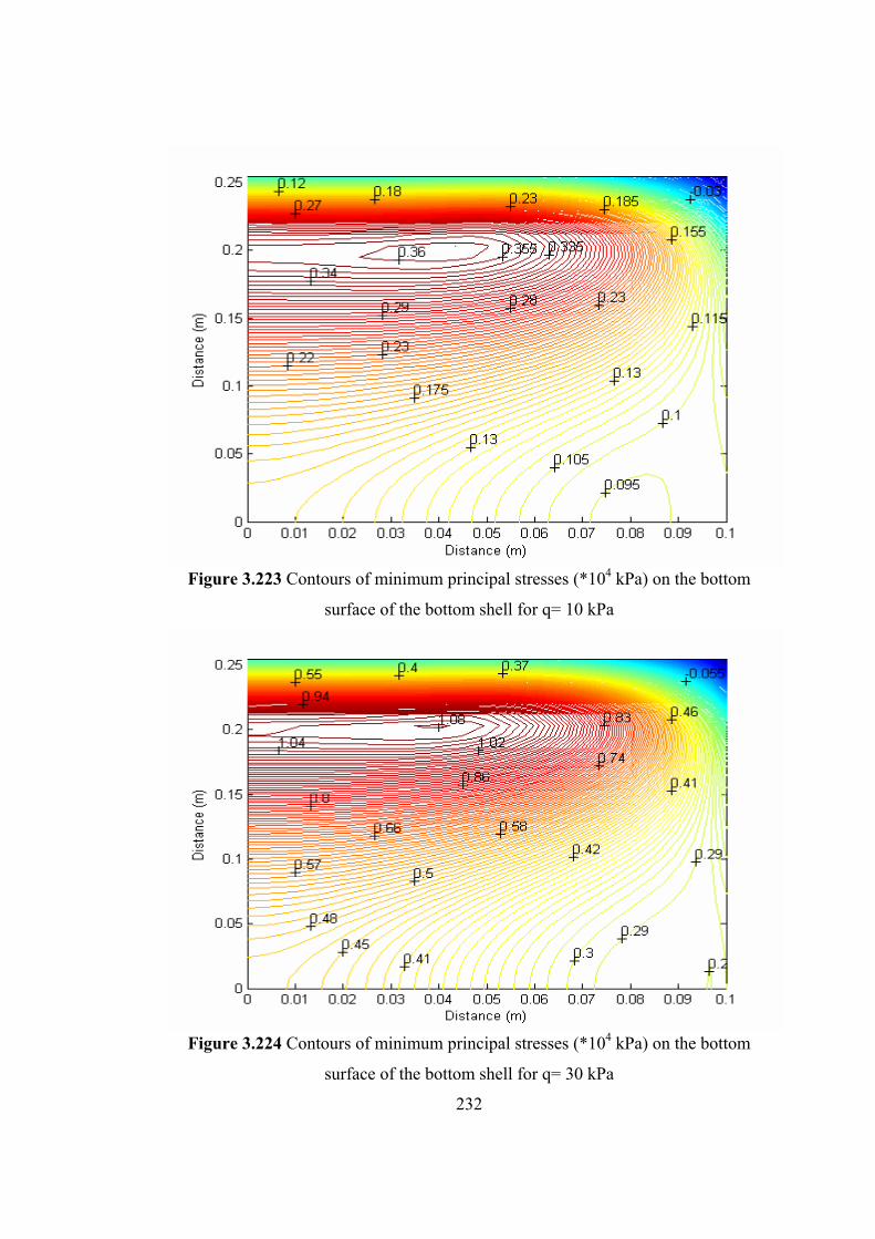
232
Figure 3.223 Contours of minimum principal stresses (*104 kPa) on the bottom
surface of the bottom shell for q= 10 kPa
Figure 3.224 Contours of minimum principal stresses (*104 kPa) on the bottom
surface of the bottom shell for q= 30 kPa
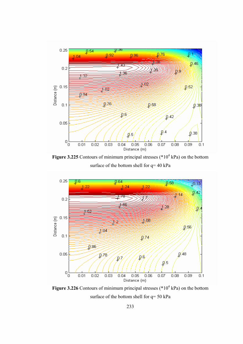
233
Figure 3.225 Contours of minimum principal stresses (*104 kPa) on the bottom
surface of the bottom shell for q= 40 kPa
Figure 3.226 Contours of minimum principal stresses (*104 kPa) on the bottom
surface of the bottom shell for q= 50 kPa
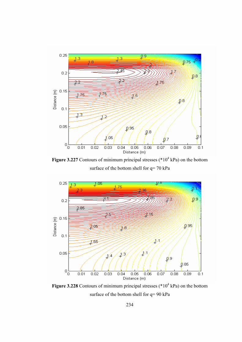
234
Figure 3.227 Contours of minimum principal stresses (*104 kPa) on the bottom
surface of the bottom shell for q= 70 kPa
Figure 3.228 Contours of minimum principal stresses (*104 kPa) on the bottom
surface of the bottom shell for q= 90 kPa
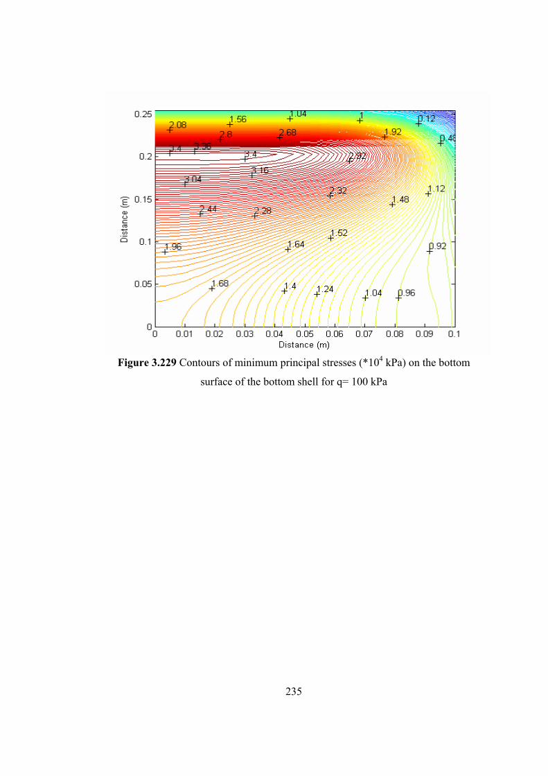
235
Figure 3.229 Contours of minimum principal stresses (*104 kPa) on the bottom
surface of the bottom shell for q= 100 kPa
236
CHAPTER 4
SUMMARY AND CONCLUSIONS
In this study, analysis of laminated glass curved beam and shell units is carried out
by using a mathematical model. Laminated glass units with two thin glass sheets and
an interlayer PVB which connects them undergo very complex and highly nonlinear
behavior under applied loads. Therefore, nonlinear theory has to be used for the true
behavior of laminated units. Nonlinearity is due to the geometry of the unit that
causes membrane stresses when the unit undergoes large deflection. The steps of the
analysis go through the stages of writing total potential energy of laminated glass
unit in terms of displacements, deriving the nonlinear governing differential
equations using variational approach and minimum potential energy theorem,
converting the nonlinear equations from continuous form to discrete form by using
finite difference method and solving the equations by using special solvers that
provide advantages in storage and computation time. For the circumferential
displacements modified strongly implicit (MSI) procedure that provides substantial
decrease in storage and computation time by storing only the finite difference
coefficients is used. To overcome the convergence difficulties variable
underrelaxation parameter is used for radial deflection w. Underrelaxation factor
helps to generate a convergent sequence for the solution and to decrease the number
of iterations to reach the solution. And also load needs to be applied in incremental
steps for the convergent solution. From the results of the analysis, it is observed that
nonlinear analysis is necessary for the true behavior of laminated glass curved beam
and shell units.
Computer programs based on the derived formulation are developed for laminated
glass curved beams and cylindrical shells. To verify the results of the developed
237
model for curved beams experimental results and finite element results are used. The
finite element model is generated and solved by using finite element package
program ABAQUS. Results of developed model reasonably agree with the finite
element results and experimental results.
The developed models are capable of simulating layered and monolithic units in
addition to the laminated units by equating shear modulus of interlayer to zero. To
determine the strength of laminated glass curved beams and shells deflections,
moments and stress functions of laminated glass unit are obtained. It is observed that
the behavior of laminated glass curved beam units approach to the behavior of
monolithic glass unit for high values of the interlayer shear modulus. The behavior of
laminated glass arch is bounded by the behavior of monolithic and layered curved
glass arches. However, these bounds are violated at some parts of the curved beam
along its length, which is not the case in the behavior of straight beams. While the
behavior of laminated glass unit is bonded by two limiting cases, which are
monolithic and layered behavior, for the fixed supported cylindrical shell, the
behavior of layered glass unit takes place between the behaviors of laminated and
monolithic units for the hinged supported cylindrical shell unit. In contrary to the
behavior of the fixed supported monolithic glass unit stress and deflection values of
the hinged supported monolithic glass unit are found to be higher than that of layered
and laminated glass units. These results are agree with the results obtained by using
the finite element method. It is possible to conclude that the monolithic systems enter
the nonlinear region later than the layered and laminated glass systems. For the
laminated glass curved beams, the effect of PVB’s shear modulus, the level of
nonlinearity, displacement, moment and stress functions are investigated. To
consider the effect of the boundary conditions to the behavior of the curved beam the
model is solved for different boundary conditions. The comparison of results are
given in figures. Nonlinearity level of simply supported beam is found to be higher
than that of fixed supported beam. Strength factor, which is employed to adjust
laminated strengths by using available design charts, is obtained for curved beams. It
is observed that strength factor of the fixed supported laminated curved beam is
238
higher than that of the simply supported beam. While the strength factor of the
simply supported curved beam is nearly 0.8, the strength factor of the fixed
supported curved beam is nearly 0.7.
Because of high nonlinearity levels, double curvature is observed for laminated
shells at high-pressure levels when applied towards to the top surface of the top glass
shell. Stress and displacement contours are plotted for laminated shell unit. Because
of nonlinearity it is observed form the figures that when the pressure is increasing,
location of maximum principal stress changes. It immigrates towards the corner of
laminated unit as the nonlinearity increases. To provide additional insight to the
behavior of laminated glass curved beams and shells strength factor which is defined
as the ratio of maximum principal stress in monolithic glass to the maximum
principal tensile stress in laminated glass is analyzed. By adjusting strength factor,
strength of laminated glass unit can be obtained by glass design charts, which are
available for monolithic and annealed glasses. Strength factor for the fixed supported
cylindrical glass shell is between 1.03-1.07, while it is between 1.15-1.16 for the
hinged supported cylindrical glass shell.
4.1 Recommendations for future work
The present model may be modified for laminated glass shells, which have curvature
in two directions. Experiments for the verification of developed model may be
conducted. The effect of delamination in the laminated glass may be investigated.
The effects of temperature, aspect ratio, interlayer thickness, glass thickness and
applied loads on the behavior of laminated curved glass beams and shells may be
studied. Dynamic model can be developed for the laminated glass curved beams and
shells. The behavior of the laminated glass shells and curved beams under impact
load may be analyzed for future studies.
239
REFERENCES
[1] Behr, R.A., Minor, J.E., Linden, M.P., Vallabhan, C.V.G. (1985). “Laminated
Glass units under uniform lateral pressure.” Journal of Structural Engineering,
111(5), 1037-1050.
[2] Behr, R.A., Linden, M.P., and Minor, J.E. (1986). “Load duration and interlayer
thickness effects on laminated glass.” Journal of Structural Engineering, 112(6),
1441-53.
[3] Behr, R.A., Karson, M.J., and Minor, J.E. (1991). “Reliability analysis of window
glass failure pressure data.” Structural Safety, 11, 43-58.
[4] Behr, R.A., Minor, J.E., Norville, H.S. (1993). “Structural behavior of
architectural laminated glass.” Journal of Structural Engineering, 119(1), 202-
222.
[5] Edel, M.T. (1997). “The effect of temperature on the bending of laminated glass
beams.” M.S. Thesis, Texas A&M University, College Station, TX.
[6] Hildebrand, F.B. (1965). “Methods of Applied Mechanics.” Prentice-Hall, Inc.,
Englewood Cliffs, N.J.
[7] Hooper, J.A. (1973). “On the bending of architectural laminated glass.” Int. J.
Mech. Sci., 15, 309-323.
[8] Langhaar, H.L. (1962). “Energy Methods in Applied Mechanics.” John Wiley and
Jones, Inc., New York.
[9] Linden, M.P., Minor, J.E., Behr, R.A., and Vallabhan, C.V.G. (1983).
“Evaluation of laterally loaded laminated glass by theory and experiment.”
Report, Glass Res. And Testing Lab., Texas Tech.
240
[10] Linden, M.P., Minor, J.E., and Vallabhan, C.V.G. (1984). “Evaluation of
laterally loaded laminated glass units by theory and experiment.” Supplemental
Report No. 1, Glass Res. And Testing Lab., Texas Tech.
[11] Minor, J.E., and Reznik, P.L. (1990). “Failure strengths of laminated glass.”
Journal of Structural Enginering, 116(4), 1030-1039.
[12] Norville, H.S., King, K.W., Swofford J.L. (1998). “Behavior and strength of
laminated glass.” Journal of Engineering Mechanics, 124(1), 46-53.
[13] Reddy, J.N. (1984). “Energy and Variational Methods in Applied Mechanics.”
John Wiley and Jones, Inc., New York.
[14] Tuzcu, İ.E. (1998). “Thickness and strength factor analyses of simply supported
laminated glass units.” M.S. Thesis, Middle East Technical University,
Ankara.
[15] Tezcan, S. (2001). “Behavior of laminated glass beams.” M.S. Thesis, Middle
East Technical University, Ankara.
[16] Vallabhan, C.V., Minor, J.E., Nagalla S.R. (1987). “Stresses in layered glass
units and monolithic glass plates.” Journal of Structural Engineering, 113(1),
36-43.
[17] Vallabhan, C.V., Ramasamudra, M. (1991). “Properties of PVB (Saflex)
interlayer used in laminated glass.” Glass Res. And Testing Lab., Texas Tech.
[18] Vallabhan, C.V., Das, Y.C, Magdi, M., Asik, M., Bailey, J.R. (1993). “Analysis
of laminated glass units.” Journal of Structural Engineering, 119(5), 1572-
1585.
[19] Van Duser, A., Jagota, A., Bennison, S.J. (1999). “Analysis of glass/polyvinyl
butyral laminates subjected to uniform pressure.” Journal of Engineering
Mechanics, 125(4), 435-442.
241
[20] Magdi, M. (1990). “Mathematical model for laminated window glass units.”
M.S. Thesis, Texas Tech University , Lubbock.
[21] Vallabhan, C.V.G., Asik, M.Z. and Kandil, K. (1997) “ Analysis of structurally
glazed systems.” Journal of Composite Structures 65(2), 231-239.
[22] Aşık, M.Z. and Vallabhan, C.V.G. (1997). “On the Convergence of Nonlinear
Plate Equations .” Computers & Structures, 65 (2), 225-229 .
[23] Asik M.Z. (2003). “Laminated Glass Plates: Revealing of Nonlinear Behavior.”
Computers & Structures, 81 (28-29), 2659-2671.
[24] Asik M.Z., Tezcan S. (2005). “ A Mathematical Model for the Behavior of
Laminated Glass Beams.” Computers & Structures, 83 (21-22), 1742-1753.
[25] Asik M.Z., Tezcan S. (2006) “ Laminated Glass Beams: Strength Factor and
Temperature Effect. ” Computers & Structures, 84, (5-6), 364-373.
[26] Asik M.Z., Dural E. (2007). “Effect of Support Conditions on the Vibration of
the Laminated Composite Beams. ” Journal of Vibration and Control, 13, (9-
10), 1361-1368.
[27] Uzhan T. (2010). “Experimental Analysis of Curved Laminated Glass Beams. ”
M.S. Thesis, Middle East Technical University, Ankara.
[28] Dawe D.J. (1974) “Numerical studies using circular arch finite elements” Computers and Structures, 4, 729-740.
[29] Rajasekaran S., Padmanabhan S. (1989). “Equations of curved beams”, Journal
of Engineering Mechanics, 115 (5), 1094-1111.
[30] Kang Y.J., You C.H., (1994) “Thin walled curved beams. 1 Formulation of
nonlinear equations. ” Journal of Engineering Mechanics, 120 (10), 2072-2100.
242
[31] Lin K.C., Heish C.M. (2007). “The closed form general solutions of 2-D curved
laminated glass beams of variable cross section” Composite Structures, 79 (4) ,
606-618.
[32] Schimmels S.A., Palazotto A.N. (1994). “Nonlinear Geometric and Material
Behavior of Shell Structures with Large Strains.” Journal of Engineering
Mechanics, 120(2), 320-345.
[33] Turkmen H.S. (1999). “Structural Response of Cylindrically Curved Laminated
Composite Shells Subjected to Blast Loading.” Journal of Sound and
Vibration, 249(4), 663-678.
[34] Aksogan O., Sofiyev A.H. (2002). “The dynamic stability of a laminated
truncated conical shell with variable elasticity moduli and densities subject to a
time-dependent external pressure.” The Journal of Strain Analysis for
Engineering Design, 37 (3), 201-210.
[35] Ugural, A.C. (1999). “Stresses in Plates and Shells.” McGraw- Hill.
[36] Timeshenko S., Krieger S.(1959) “Theory of Plates and Shells.” McGraw- Hill.
[37] Palazotto A.N., Dennis S.T. (1992). “Nonlinear Analysis of Shell Structures.”
American Institute of Aeronautics and Astronautics.
[38] Palani G.S., Rajasekaran S. (1992). “Finite element analysis of thin walled
curved beams made of composites” Journal of Structural Engineering, 118 (8),
2039-2062.
243
CURRICULUM VITAE
PERSONAL INFORMATION
Surname, Name: Dural, Ebru Nationality: Turkish (TC) Date and Place of Birth: 10 March 1979, Erzurum Marital Status: Married Phone: +90 312 210 44 57 Fax: +90 312 210 44 62 email: [email protected] EDUCATION Degree Institution Year of Graduation
BS Ataturk University Civil Engineering 2002
High School Mehmet Akif Ersoy High School, Erzurum 1997
WORK EXPERIENCE
Year Place Enrollment
2002-Present METU Department of Engineering Sciences Research Assistant
PUBLICATIONS
1. Asik, M.Z., and Dural, E. (2006). “Effect of Support Conditions on the Vibration
of the Laminated Composite Beams.” Mathematical Methods in Engineering
International Symposium.
2. Asik, M.Z., and Dural, E. (2006). “A Mathematical Model for the Nonlinear
Analysis of a Laminated Cylindrical Glass Shells.” 7th World Congress on
Computational Mechanics, Los Angeles, USA.
3. Asik, M.Z., Dural, E. and Bayar, G. (2007). “Nonlinear Analysis of a Laminated
Glass Arch.”, 3rd International Conference on Structural Engineering, Mechanics
and Computation, Cape Town, South Africa.
244
4. Asik, M.Z., and Dural, E. (2008). “A Computational Model For The Prediction Of
The Nonlinear Behavior Of a Laminated Cylindrical Glass Shell.”, The 15th ICCES
Conference, Hawai, USA.
5. Asik, M.Z., and Dural, E. (2008). “Effect of Support Conditions on the Behavior of
the Laminated Glass Arch.”, 8th World Congress on Computational Mechanics, 5th.
European Congress on Computational Methods in Applied Sciences and
Engineering, Venice, Italy.
6.Dural, E and Asik, M.Z. (2009). “Kompozit Cam Eğrisel Kirişlerin Doğrusal
Olmayan Davranışları.” XVI. Ulusal Mekanik Kongresi, Kayseri, Turkey.
7. Asik, M.Z., and Dural, E. (2010). “Nonlinear Analysis of a Laminated Cylindrical
Glass Shell.” The Ninth International Congress on Advances in Civil Engineering,
Trabzon, Turkey.
8. Asik, M.Z., and Dural, E. (2006). “Effect of Support Conditions on the Vibration
of the Laminated Composite Beams.” Journal of Vibration and Control September
2007 vol. 13 no. 9-10 1361-1368.
9. Asik, M.Z., Dural, E. , Uzhan, T. and Yetmez, M.(2010). “Experimental and
Mathematical Analysis of Curved Laminated Glass Beam.” International Conference
on Theoretical, Applied, Computational and Experimental Mechanics
, IIT Kharagpur, India
HOBBIES
Swimming, Reading, Computer Technologies, Movies, Music