Analysis of microarray data

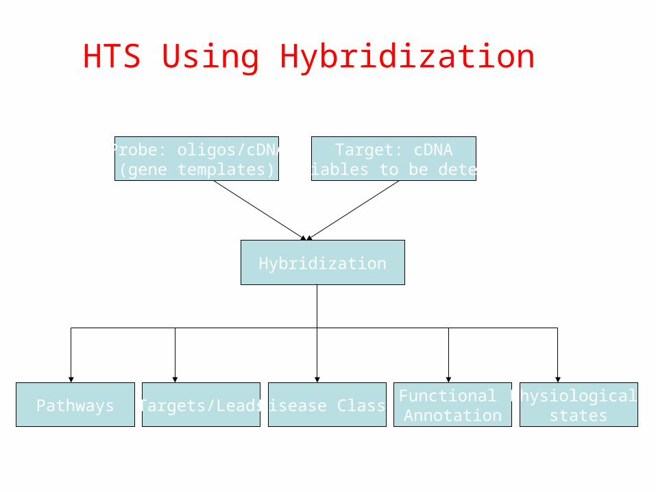
HTS Using Hybridization

Target: cDNA (variables to be detected)

Probe: oligos/cDNA(gene templates) +

Hybridization

PathwaysFunctional Annotation

Analysis of outcome

Microarray Chip

Samples

Targets/Leads Disease Class.Physiological

states

Timeline for drug discovery

Discovery (5 yrs)5000 Gene expression

study

Pre-Clinical (1 yr)

50

Clinical (6 yrs)

5

Review (2 yrs)

1

Marketed

Microarray for Yeast

Figure from DeRisi et al. (See next slide).

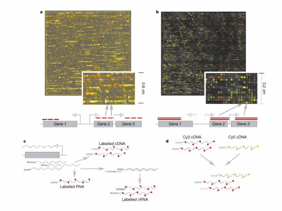
cDNA Microarrays

• Use robot to spot glass slides at precise points with complete gene/EST sequences

• Able to measure qualitatively relative expression levels of genes

– Differential expression by use of simultaneous, two-colour fluorescence hybridisation

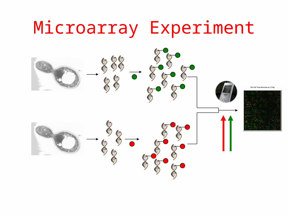
Microarray Experiment

RT-PCR

RT-PCR

LASER

DNA “Chip”

High glucose

Low glucose

Microarray for Yeast

Figure from DeRisi et al. (See next slide).

cDNA Microarrays

• Use robot to spot glass slides at precise points with complete gene/EST sequences

• Able to measure qualitatively relative expression levels of genes

– Differential expression by use of simultaneous, two-colour fluorescence hybridisation

Microarray Experiment

RT-PCR

RT-PCR

LASER

DNA “Chip”

High glucose

Low glucose

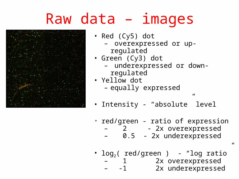
Raw data – images• Red (Cy5) dot

– overexpressed or up-regulated• Green (Cy3) dot

– underexpressed or down-regulated• Yellow dot

– equally expressed

• Intensity - “absolute” level

• red/green - ratio of expression– 2 - 2x overexpressed– 0.5 - 2x underexpressed

• log2( red/green ) - “log ratio”– 1 2x overexpressed– -1 2x underexpressed

cDNA plotted microarray

Microarray Expression Value Representation

expression value types

primary images composite imagese.g., green/red ratios

primaryspots

compositespots

primarymeasurements

derivedvalues

Source: MGED

Analysing Expression Data

• Measure gene expression levels under various conditions

– The more experiments the finer the classification

• Clustering reveals groupings of genes and/or experiments / tissues / treatments

– Hypothesize similar regulatory mechanisms and perhaps role

• Analysis of expression data needs to be integrated with other types of biological analysis and knowledge

Gene 1

Gene 2

Gene n

Condition 1 Condition m

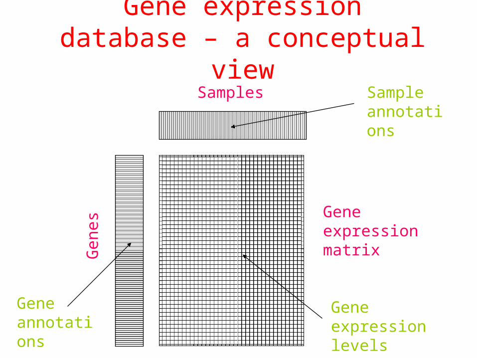
Gene expression database – a conceptual view

SamplesG

enes

Gene expression levels

Sample annotations

Gene annotations

Gene expression matrix

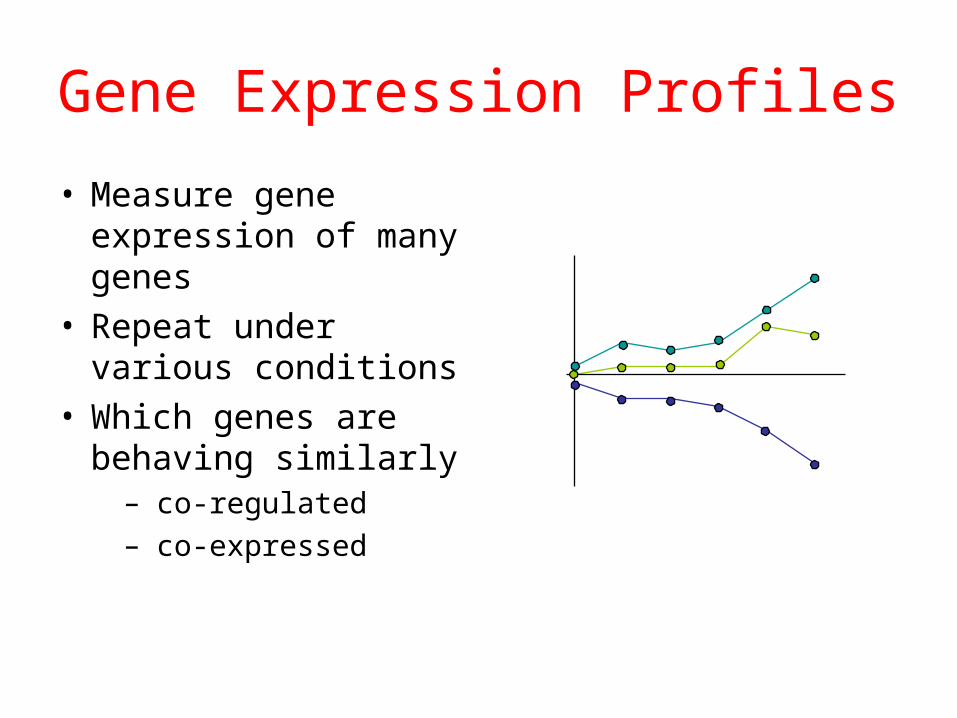
Gene Expression Profiles

• Measure gene expression of many genes

• Repeat under various conditions

• Which genes are behaving similarly

– co-regulated– co-expressed

Bioinformatics in microarray data

• Array design

• Data extraction (Pixel to matrix)

• Background correction

• Data normalization

• Data analysis

Data normalization

expression of gen x in experiment i expression of gen x in reference

Logarithm of ratio - treats induction and repression of identical

magnitude as numerical equal but with opposite sign.

Xi log(Ei / Ri).

Levels of analysis

Level 1: Which genes are induced / repressed? Gives a good understanding of the biology.

Methods: Factor-2 rule, t-test.Level 2: Which genes are co-regulated? Inference of function.

-Clustering algorithms,-Support Vector Machines.

Level 3: Which genes regulate others? Reconstruction of networks.

- Transcriptions factor binding sites,- Bayesian networks.

Analysis of multiple experiments

Xi log(Ei / Ri).

.,...,1 XX m

X

Expression of gene x in m experiments can berepresented by an exression vector with m elementer

1) The vector can be normalized so that = 0, 2 = 1 Gener whith low expression and low variation can be correlated to gens with high expression and high variation.2) Discretization: up regulation: +1

no regulation: 0down regulation: -1

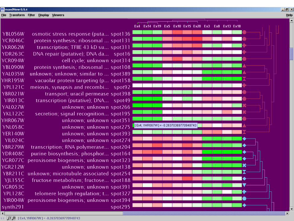
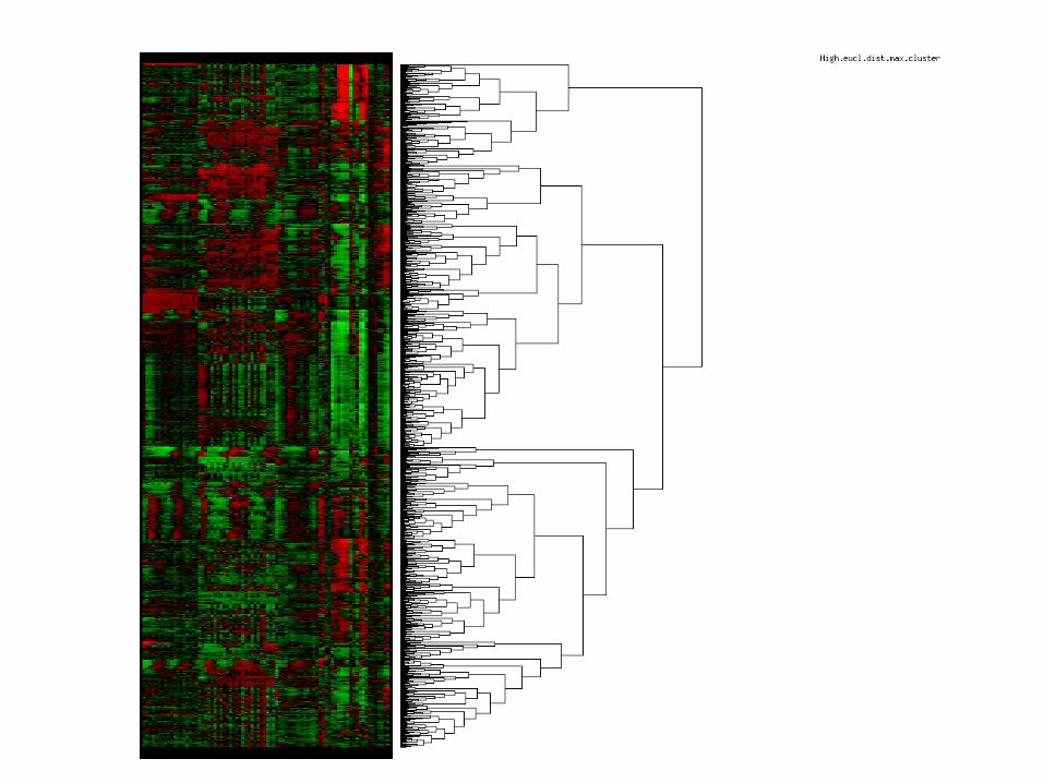
Clustering

Hierachical clustering: - Transforms n (genes) * m (experiments) matrix into a diagonal n * n similarity (or distance) matrix

Similarity (or distance) measures:Euclidic distancePearsons correlation coefficent

Ud fra denne matrix kan man bygge et dendrogram, ved

Eisen et al. 1998 PNAS 95:14863-14868

Key Terms in Cluster Analysis

• Distance & Similarity measures

• Hierarchical & non-hierarchical

• Single/complete/average linkage

• Dendrograms & ordering

Distance Measures: Minkowski Metric

r rp

iii

p

p

yxyxd

yyyy

xxxx

pyx

||),(

)(

)(

1

21

21

by defined is metric Minkowski The

:features have both and objects two Suppose

Most Common Minkowski Metrics

||max),(

||),(

1

||),(

2

1

1

2 2

1

iipi

p

iii

p

iii

yxyxd

r

yxyxd

r

yxyxd

r

) distance sup"(" 3,

distance) (Manhattan 2,

) distance (Euclidean 1,

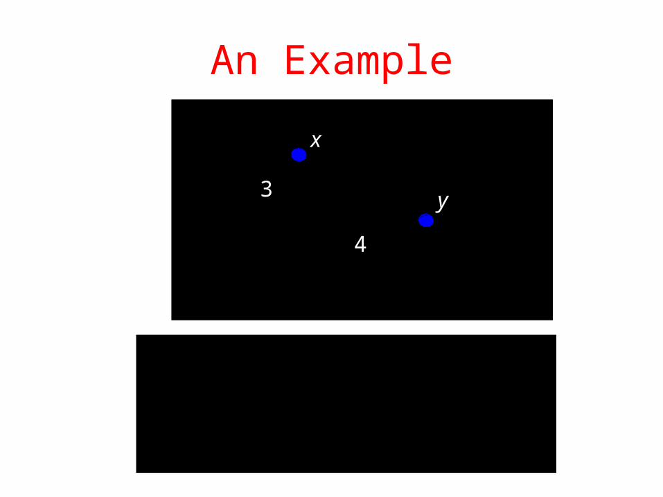
An Example

.4}3,4{max

.734

.5342 22

:distance sup"" 3,

:distance Manhattan 2,

:distance Euclidean 1,

4

3

x

y

Taken from http://www.icgeb.trieste.it/~netsrv/courseware/biorithms/index.htm

Similarity Measures: Correlation Coefficient

. and :averages

)()(

))((),(

1

1

1

1

1 1

22

1

p

iip

p

iip

p

i

p

iii

p

iii

yyxx

yyxx

yyxxyxs

1),( yxs

Similarity Measures: Correlation Coefficient

Time

Gene A

Gene B Gene A

Time

Gene B

Expression LevelExpression Level

Expression Level

Time

Gene A

Gene B

Distance-based Clustering

• Assign a distance measure between data • Find a partition such that:

– Distance between objects within partition (i.e. same cluster) is minimized

– Distance between objects from different clusters is maximised

• Issues :– Requires defining a distance (similarity) measure in situation

where it is unclear how to assign it– What relative weighting to give to one attribute vs another?– Number of possible partition is super-exponential

Hierarchical Clustering Techniques

At the beginning, each object (gene) is a cluster. In each of the subsequent steps, two closest clusters will merge into one cluster until there is only one cluster left.

Hierarchical ClusteringGiven a set of N items to be clustered, and an NxN distance (or similarity) matrix, the basic process hierarchical clustering is this:

1.Start by assigning each item to its own cluster, so that if you have N items, you now have N clusters, each containing just one item. Let the distances (similarities) between the clusters equal the distances (similarities) between the items they contain.

2.Find the closest (most similar) pair of clusters and merge them into a single cluster, so that now you have one less cluster.

3.Compute distances (similarities) between the new cluster and each of the old clusters.

4.Repeat steps 2 and 3 until all items are clustered into a single cluster of size N.

The distance between two clusters is defined as the distance between

• Single-Link Method / Nearest Neighbor (NN): minimum of pairwise dissimilarities

• Complete-Link / Furthest Neighbor (FN): maximum of pairwise dissimilarities

• Unweighted Pair Group Method with Arithmetic Mean (UPGMA): average of pairwise dissimilarities

• Their Centroids.• Average of all cross-cluster pairs.

Computing Distances• single-link clustering (also called the connectedness or minimum method) : we consider the distance between one cluster and another cluster to be equal to the shortest distance from any member of one cluster to any member of the other cluster. If the data consist of similarities, we consider the similarity between one cluster and another cluster to be equal to the greatest similarity from any member of one cluster to any member of the other cluster.

• complete-link clustering (also called the diameter or maximum method): we consider the distance between one cluster and another cluster to be equal to the longest distance from any member of one cluster to any member of

the other cluster.

• average-link clustering : we consider the distance between one cluster and another cluster to be equal to the average distance from any member of one cluster

to any member of the other cluster.

Single-Link Method

ba

453652

cba

dcb

Distance Matrix

Euclidean Distance

453,

cba

dc

453652

cba

dcb4,, cbad

(1) (2) (3)

a,b,ccc d

a,b

d da,b,c,d

Complete-Link Method

ba

453652

cba

dcb

Distance Matrix

Euclidean Distance

465,

cba

dc

453652

cba

dcb6,,

badc

(1) (2) (3)

a,b

cc d

a,b

d c,da,b,c,d

Compare Dendrograms

a b c d a b c d

2

4

6

0

Single-Link Complete-Link

Ordered dendrograms

2 n-1 linear orderings of n elements (n= # genes or conditions)

Maximizing adjacent similarity is impractical. So order by:•Average expression level, •Time of max induction, or•Chromosome positioning

Eisen98

Serum stimulation of human fibroblasts (24h) Cholesterol biosynthesis

Celle cyclusI-E responseSignalling/ Angiogenesis

Wound healning

k-means clustering

Tavazoie et al. 1999 Nature Genet. 22:281-285

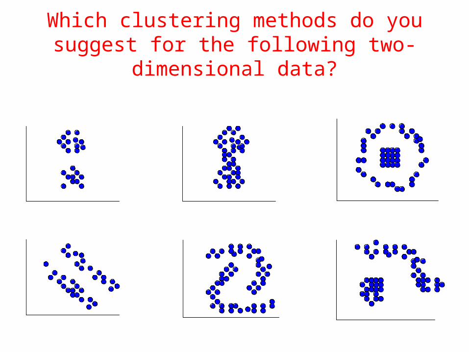
Which clustering methods do you suggest for the following two-dimensional data?

Clustering by K-means

•Given a set S of N p-dimension vectors without any prior knowledge about the set, the K-means clustering algorithm forms K disjoint nonempty subsets such that each subset minimizes some measure of dissimilarity locally. The algorithm will globally yield an optimal dissimilarity of all subsets. •K-means algorithm has time complexity O(RKN) where K is the number of desired clusters and R is the number of iterations to converges.

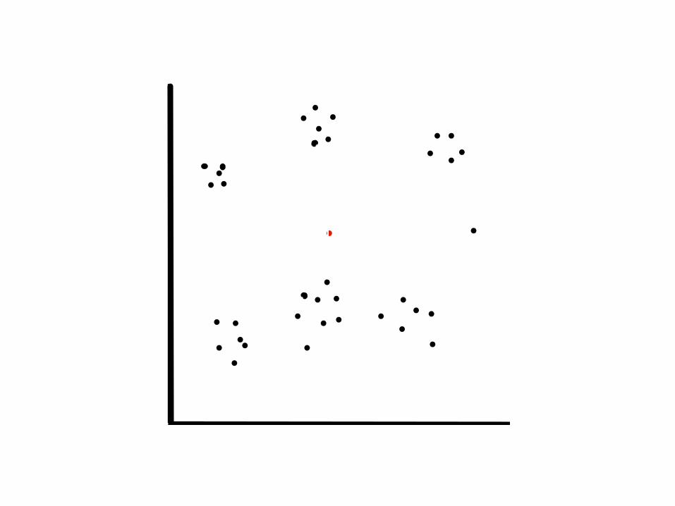
•Euclidean distance metric between the coordinates of any two genes in the space reflects ignorance of a more biologically relevant measure of distance. K-means is an unsupervised, iterative algorithm that minimizes the within-cluster sum of squared distances from the cluster mean. •The first cluster center is chosen as the centroid of the entire data set and subsequent centers are chosen by finding the data point farthest from the centers already chosen. 200-400 iterations.

K-Means Clustering Algorithm

1) Select an initial partition of k clusters

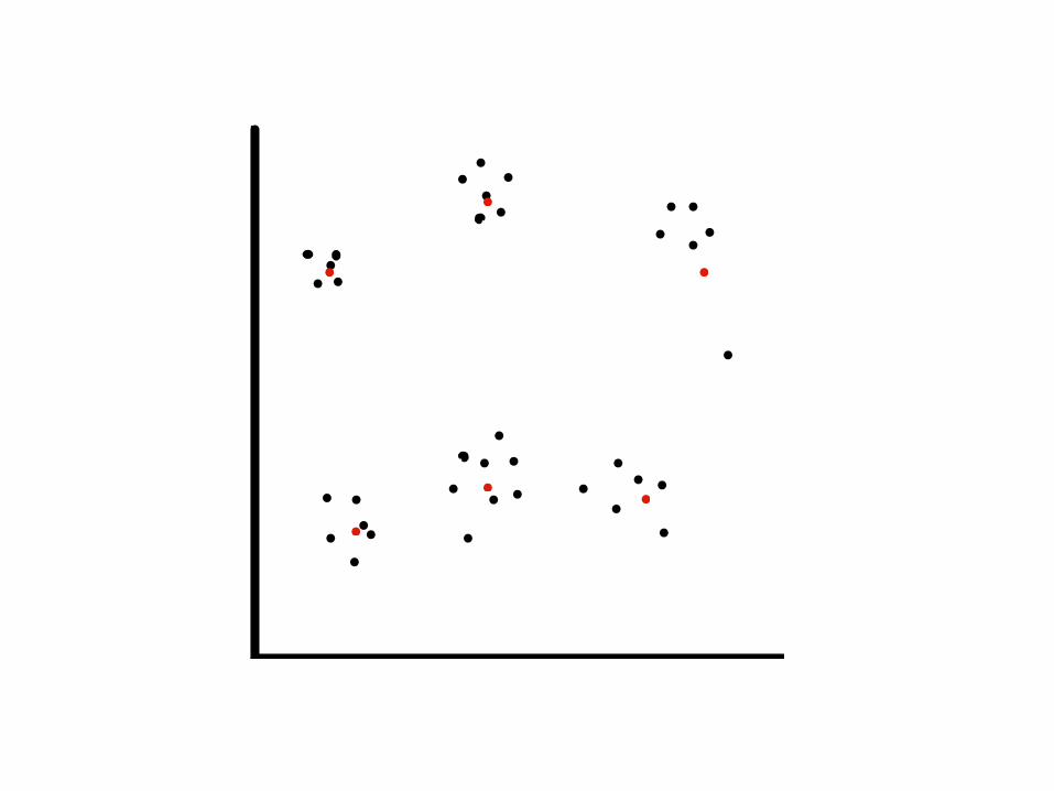
2) Assign each object to the cluster with the closest center:

3) Compute the new centers of the clusters:

4) Repeat step 2 and 3 until no object changes cluster

SXXnXSC n

n

ii

,...,,/)( 1

1

1. centroide

1. centroide

2. centroide

3. centroide

4. centroide

5. centroide

6. centroide

k = 6

1. centroide

2. centroide

3. centroide

4. centroide

5. centroide

6. centroide

k = 6

1. centroide2. centroide

3. centroide

4. centroide

5. centroide

6. centroide

k = 6

Self organizing maps

Tamayo et al. 1999 PNAS 96:2907-2912

1. centroide 2. centroide 3. centroide

4. centroide 5. centroide 6. centroide

k = 6

k = 6

k = 6

k = 6

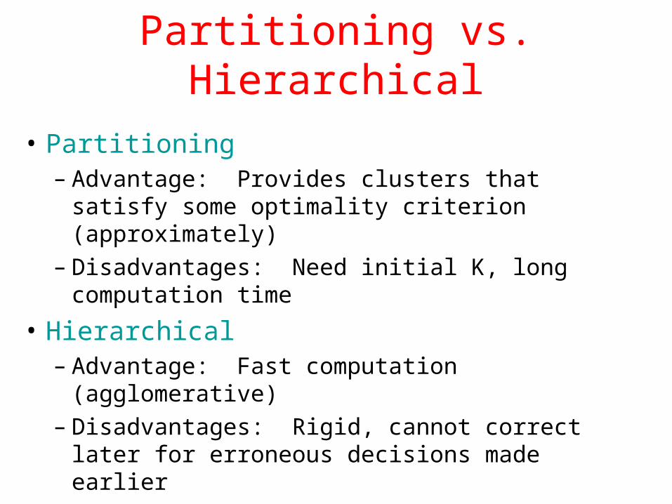
Partitioning vs. Hierarchical

• Partitioning– Advantage: Provides clusters that satisfy some

optimality criterion (approximately)– Disadvantages: Need initial K, long computation

time

• Hierarchical– Advantage: Fast computation (agglomerative)– Disadvantages: Rigid, cannot correct later for

erroneous decisions made earlier

Generic Clustering Tasks

• Estimating number of clusters

• Assigning each object to a cluster

• Assessing strength/confidence of cluster assignments for individual objects

• Assessing cluster homogeneity

Clustering and promoter elements

Harmer et al. 2000 Science 290:2110-2113

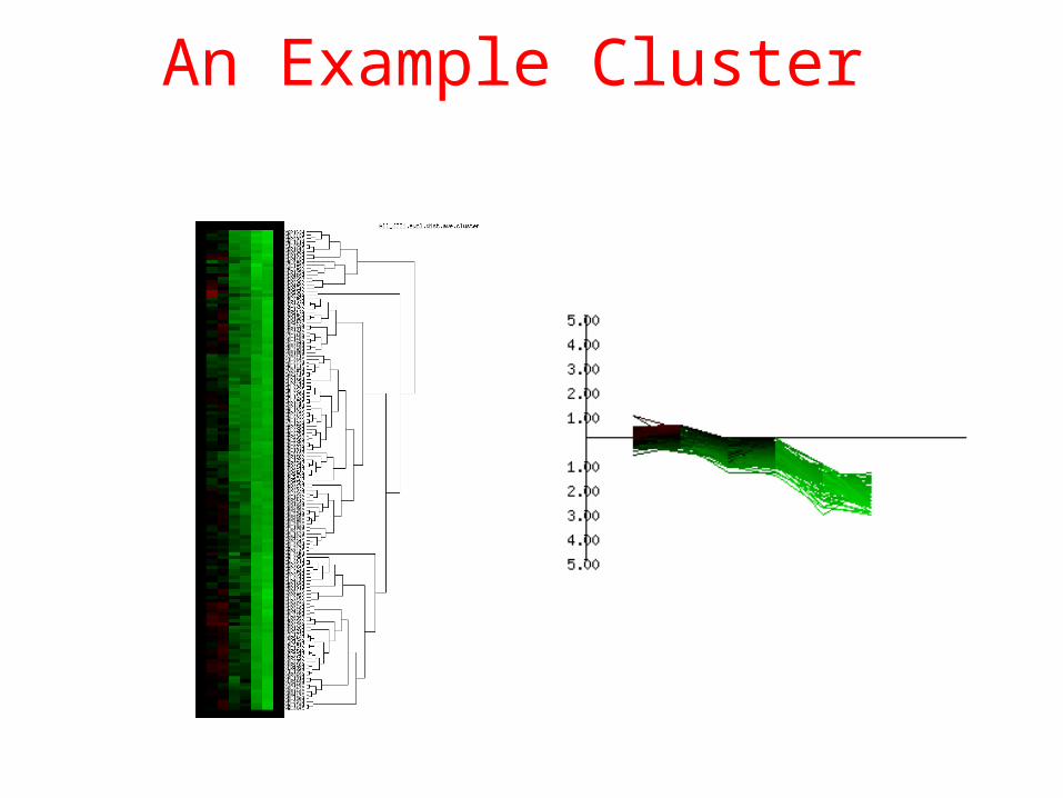
An Example Cluster

(DeRisi et al, 1997)

Cluster of co-expressed genes, pattern discovery in regulatory regions

600 basepairs

Expression profiles

Upstream regions

Retrieve

Pattern over-represented in cluster

Some Discovered PatternsPattern Probability Cluster No. TotalACGCG 6.41E-39 96 75 1088ACGCGT 5.23E-38 94 52 387CCTCGACTAA 5.43E-38 27 18 23GACGCG 7.89E-31 86 40 284TTTCGAAACTTACAAAAAT 2.08E-29 26 14 18TTCTTGTCAAAAAGC 2.08E-29 26 14 18ACATACTATTGTTAAT 3.81E-28 22 13 18GATGAGATG 5.60E-28 68 24 83TGTTTATATTGATGGA 1.90E-27 24 13 18GATGGATTTCTTGTCAAAA 5.04E-27 18 12 18TATAAATAGAGC 1.51E-26 27 13 18GATTTCTTGTCAAA 3.40E-26 20 12 18GATGGATTTCTTG 3.40E-26 20 12 18GGTGGCAA 4.18E-26 40 20 96TTCTTGTCAAAAAGCA 5.10E-26 29 13 18

Vilo et al. 2001

Results

• Over 6000 “interesting” patterns• Many from homologous upstreams - Removed

– Leaves 1500 patterns

• These patterns clustered into 62 groups– Found alignments, consensus, and profiles

• Of 62 clusters - 48 had patterns matching SCPD (experimentally mapped) binding site database

Jaak Vilo

Jaak Vilo

The "GGTGGCAA" Cluster ORF Gene Description

YBL041W PRE7 20S proteasome subunit(beta6) YBR170C NPL4 nuclear protein localization factor and ER translocation component YDL126C CDC48 microsomal protein of CDC48/PAS1/SEC18 family of ATPases YDL100C similarity to E.coli arsenical pump-driving ATPase YDL097C RPN6 subunit of the regulatory particle of the proteasome YDR313C PIB phosphatidylinositol(3)-phosphate binding protein YDR330W similarity to hypothetical S. pombe protein YDR394W RPT3 26S proteasome regulatory subunit YDR427W RPN9 subunit of the regulatory particle of the proteasome YDR510W SMT3 ubiquitin-like protein YER012W PRE1 20S proteasome subunit C11(beta4) YFR004W RPN11 26S proteasome regulatory subunit YFR033C QCR6 ubiquinol--cytochrome-c reductase 17K protein YFR050C PRE4 20S proteasome subunit(beta7) YFR052W RPN12 26S proteasome regulatory subunit YGL048C RPT6 26S proteasome regulatory subunit YGL036W MTC2 Mtf1 Two hybrid Clone 2 YGL011C SCL1 20S proteasome subunit YC7ALPHA/Y8 (alpha1) YGR048W UFD1 ubiquitin fusion degradation protein YGR135W PRE9 20S proteasome subunit Y13 (alpha3) YGR253C PUP2 20S proteasome subunit(alpha5) YIL075C RPN2 26S proteasome regulatory subunit YJL102W MEF2 translation elongation factor, mitochondrial YJL053W PEP8 vacuolar protein sorting/targeting protein YJL036W weak similarity to Mvp1p YJL001W PRE3 20S proteasome subunit (beta1) YJR117W STE24 zinc metallo-protease YKL145W RPT1 26S proteasome regulatory subunit YKL117W SBA1 Hsp90 (Ninety) Associated Co-chaperone YLR387C similarity to YBR267w YMR314W PRE5 20S proteasome subunit(alpha6) YOL038W PRE6 20S proteasome subunit (alpha4) YOR117W RPT5 26S proteasome regulatory subunit YOR157C PUP1 20S proteasome subunit (beta2) YOR176W HEM15 ferrochelatase precursor YOR259C RPT4 26S proteasome regulatory subunit YOR317W FAA1 long-chain-fatty-acid--CoA ligase YOR362C PRE10 20S proteasome subunit C1 (alpha7) YPR103W PRE2 20S proteasome subunit (beta5) YPR108W RPN7 subunit of the regulatory particle of the proteasome

From Gifford 2001 Science 293:2049-205034 genes, 140 experiments

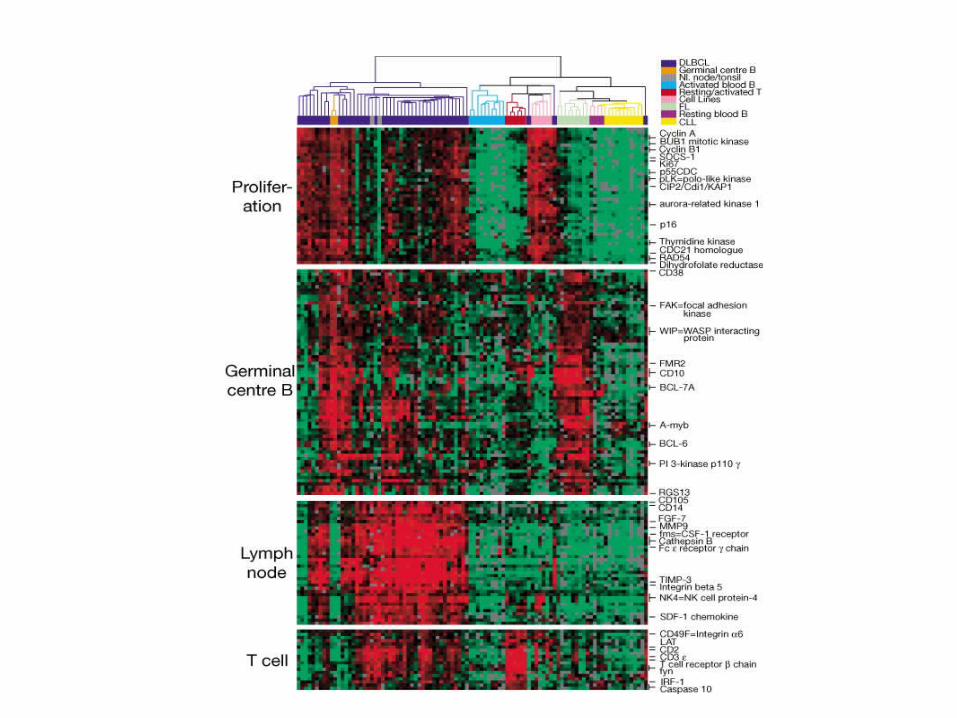
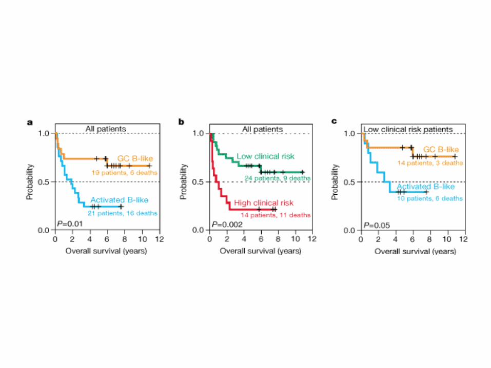
Two sided clustering

Alizadeh et al. 2000 Nature 403:505-5011

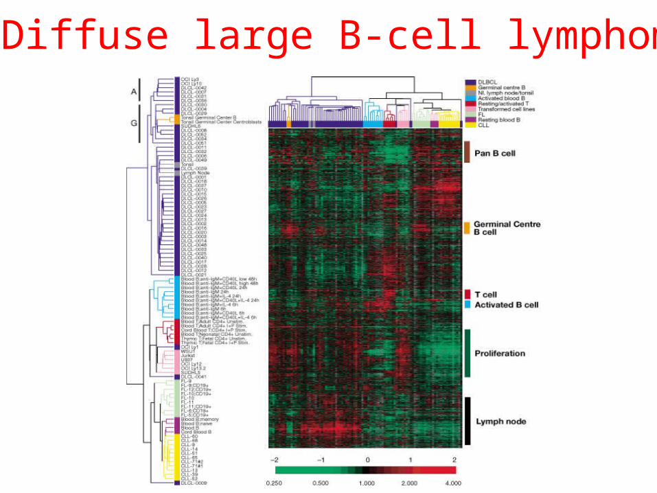
Diffuse large B-cell lymphoma

Principal Component Analysis

(Singular Value Decomposition) Alter et al. 2000 PNAS 97:10101-10106

Bayesian Networks Analysis

Friedman et al. 2000 J. Comp. Biol., 7:601-620

P(X1,..., Xn ) P(Xi PaG( Xi)).i1

n

- Kan kun representere acykliske relationer.

Principal Component Analysis

ˆ e ˆ u ̂ ̂ v T .

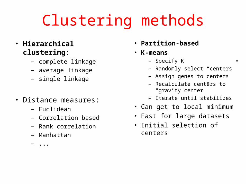
Clustering methods

• Hierarchical clustering:– complete linkage– average linkage– single linkage

• Distance measures:– Euclidean– Correlation based– Rank correlation– Manhattan– ...

• Partition-based• K-means

– Specify K– Randomly select “centers”– Assign genes to centers– Recalculate centers to

“gravity center”– Iterate until stabilizes

• Can get to local minimum• Fast for large datasets• Initial selection of centers