Analysis of Model-driven vs. Data-driven Approaches to Engaging Student Learning in Introductory Geoscience Laboratories

Laura A. Lukes

Thesis submitted to the faculty of the Virginia Polytechnic Institute and State University

in partial fulfillment of the requirements for the degree of

Master of Science in

Geosciences

Barbara Bekken, Chair Susan Eriksson James Spotila

6 May 2004 Virginia Polytechnic Institute and State University

Blacksburg, Virginia

Keywords: (Education - Undergraduate, Education (general), Geoscience, Plate Tectonics, Surficial Geology, History & Philosophy of Science, Geochronology, Areal Geology, Geology) Copyright 2004, Laura A. Lukes.

Analysis of Model-driven vs. Data-driven Approaches to Engaging Student Learning in Introductory Geoscience Laboratories

Laura A. Lukes

Abstract

Increasingly, teachers are encouraged to use data resources in their classrooms, which are

becoming more widely available on the web through organizations such as Digital Library for Earth System Education, National Science Digital Library, Project Kaleidoscope, and the National Science Teachers Association. As "real" data becomes readily accessible, studies are needed to assess and describe how to effectively use data to convey both content material and the nature of scientific inquiry and discovery. In this study, we created two introductory undergraduate physical geology lab modules for calculating plate motion. One engages students with a model-driven approach using contrived data. Students are taught a descriptive model and work with a set of contrived data that supports the model. The other lab exercise uses a data-driven approach with real data. Students are given the real data and are asked to make sense of it. They must use the data to create a descriptive model. Student content knowledge and understanding of the nature of science were assessed in a pretest-posttest experimental design using a survey containing 11 Likert-like scale questions covering the nature of science and 9 modified true/false format questions covering content knowledge. Survey results indicated that students gained content knowledge and increased their understanding of the nature of science with both approaches. Lab observations and written interviews indicate these gains resulted from students experiencing different pedagogical approaches used in each of the two labs.

Dedication

To my grandparents, who both passed away while I was working on this degree. Without their involvement in my life, I would have never had the strength to follow my dreams.

To my mom, who always provided a map showing the way with exits clearly labeled, just in

case...

iii

Acknowledgements

I would like to thank the Department of Geosciences at Virginia Tech and my committee for making this unique project possible. The National Science Foundation (EAR 02229628)

indirectly provided funding for my early research on the San Andreas.

iv

Table of Contents

List of Tables and Figures - p. vi Preface - p.1 Introduction - p. 3 Using data in the classroom - p. 4 Methods - p. 6 Results - p. 16 Discussion - p. 29 Implications - p. 32 References - p. 33 Appendices - p. 36

v

List of Tables and Figures Table 1- Nature of science survey questions - p. 7 Table 2- Content survey questions - p. 8 Table 3- Highlights of Session I demographics - p. 11 Table 4- Highlights of Session II demographics - p. 13 Table 5- Significant mean changes, data-driven population - p. 18 Table 6- Significant mean changes, model-driven population - p. 24 Figure 1- Nature of science results, Session I - p. 17 Figure 2- Content results by question, Session I - p. 20 Figure 3- Content results by total score, Session I - p. 21 Figure 4- Nature of science results, Session II - p. 23 Figure 5- Content results by question, Session II - p. 26 Figure 6- Content results by total score, Session I - p. 27

vi

Preface A study of this nature is unprecedented in the Department of Geosciences here at Virginia Tech. As a result, I felt it was worthwhile to offer a brief explanation of how this study came to fruition. My Master’s research project began with an investigation of the mechanisms and rates of uplift within the San Andreas Fault zone (SAF) in southern California under the tutelage of Jim Spotila. The overall goal of the project was to test different models of transpression by examining uplift rates along a section of the SAF that was both oblique to regional plate motion and free of local geometrical anomalies. The presence of any local geometrical anomalies could cause a localized transpression effect, thus potentially undermining the validity of regional transpression models.

The Portal Ridge/Leona Valley area in southern CA was chosen as such a test site because: 1) it is located in the “Big Bend” region of the SAF, which is approximately 27 degrees oblique to regional plate motion as determined by NUVEL-1A data and 2) has no known local geometrical fault anomalies. The plan was to establish/constrain the rock uplift history of the area and compare it to other areas along the fault, thus providing evidence to support or refute existing models of transpression. We would constrain exhumation rates in the Portal Ridge/Leona Valley area by approximating rock uplift rates using (U-Th)/He dating of exposed granite and gneiss samples. A field reconnaissance trip was made in spring 2003. We observed geomorphic surfaces, noted potential structural evidence of recent uplifts, and collected samples for dating. I spent the summer of 2003 reading journal articles about models for transpression and (U-Th)/He dating techniques. I began to think about the uncertainties associated with science and how we, as students, are taught to deal with datasets in general. To me, the SAF project seemed to be aimed at collecting a dataset and determining the model of transpression which best “fit” the data. This approach seemed strikingly similar to what I remembered learning to do with data in school. In lab assignments, my fellow students and I would be asked to collect and analyze data. That data should, we were told, work out in support of the predetermined model being taught in class that week. We were constantly aware of the "end product" that the data supported. This idea and approach, however, seemed counterintuitive and in direct conflict with that which I remember being taught in school about scientific methods and science’s purported objectivity. That is, the scientific method tells us that we should observe, test, and conclude/ propose our own model based on our data, rather than trying to use the data to get to a predicted conclusion.

In reality, the SAF project was approaching the problem using scientific methods. We were asking, "How is transpression being accommodated along the SAF?" Our objectives included collecting data that could be used to propose a hypothesis for how transpression was being accommodated. Once this hypothesis was constrained by the data, then it could be compared with existing hypotheses. I was having difficulty reconciling the differences between the investigative approach the study was actually employing and the model-driven approach I had been taught in school. I found myself wrestling more with the nature of science than with the SAF problem itself. This preoccupation, combined with my increasing interest and passion for both teaching and learning philosophies, led me into the study outlined and presented in this paper. To ensure that my time spent investigating the SAF was incorporated into my new research direction, the

1

SAF topic provided the geologic subject of the treatment lab assignments in this project. Jim Spotila’s research team is still pursuing the SAF project. Since my departure from the project, the samples from the field reconnaissance trip, which I participated in, have been processed and are currently under investigation (Spotila et al, 2003).

2

Introduction The National Science Education Standards (1996) focused on the need for science

literacy in students (National Research Council, 1996). The standards clearly outline and define science literacy as it relates to Earth science, emphasizing the link between science literacy and student inquiry through work with data (National Research Council, 1996). The geoscience education community has in turn provided data-rich resources for use in the classroom to promote science literacy, through such programs as Digital Library for Earth System Education, National Science Digital Library, and Project Kaleidoscope. However, as National Science Foundation's Geoscience Education: A Recommended Strategy report notes, there remains uncertainty regarding how students can most effectively learn from these increasingly available resources because, according to Somerville (1997), a gap exists in our research knowledge of geoscience education at every level.

The heightened emphasis on using data to improve science literacy in students has inspired a culture of buzzwords and phrases in the geoscience education community that work to connect science literacy with the data resources available to educators, including teachers at the undergraduate level. These phrases, such as "data-rich experiences" and "using data in the classroom" (DLESE, 2003?), are road signs for teachers trying to keep up with the standards, guiding them to the appropriate data-rich resources and guidelines for using them. Currently within these resources, a data-rich classroom experience has been defined rather broadly to include the use of raw, derived and/or simulated data (DLESE, 2003?), making it unclear which types of data are the most effective tools to use in "data-rich experiences." This ambiguity combined with the community's reliance on anecdotal evidence for effective teaching methods in Earth sciences (Somerville, 1997) has lead us to investigate the effectiveness of different types of data-rich experiences and their components, namely the different approaches to using data and the different types of data.

The goals of this study are three fold. First, we aim to constrain the definition of an effective data-rich experience in reference to Earth science education. Second, we plan to provide formal evidence, both qualitative and quantitative, of the benefits of engaging students with data. And lastly, we hope to suggest effective ways to use data in established curricula. To achieve these goals, we evaluated and compared the effectiveness of using a data-driven approach with real scientific data to a model-driven approach with contrived data in two separate two-week lab modules. We assessed whether either format resulted in significantly better gains in the student understanding of the nature of science. Additionally, we compared the effectiveness of both types of data and their associated approaches at conveying content knowledge to students. We noted if real data, because of its nature, clarified or confused content knowledge, as compared to contrived data, which is designed to lead students to a specific conceptual model that encompasses only the content knowledge for which the students are responsible. We used the results to further define how to use datasets whether real or contrived more effectively in the classroom.

3

Using data in the classroom In general, data that are used in the classroom can be split readily into two end-member

groups: real and contrived. The difference between the two data types lies in their method of construction. Real data are data that have been collected in order to investigate something; these data contain outliers, errors, and variability. Contrived data are either real data that have been simplified or streamlined or are data that have been created altogether. Defining data this way is incomplete, however, because data are meaningless unless they serve some purpose and are used as a means to an end.

In terms of education and using data in the classroom, the definition of data types must therefore incorporate the way in which the data are used. This brings up the data-model connection that is briefly addressed by the National Science Education Standards (National Research Council, 1996). In general, data are used in one of two ways in a classroom setting. Either data are used to support a conceptual or descriptive model or they are used to support the process of recognizing trends and patterns that will lead to a model. In other words, the connection between the data and the model can be either model-driven (the former) or data-driven (the latter).

Science teachers, including those at the undergraduate level, tend to teach models. Commonly, they incorporate data into their curricula by employing a model-driven approach. In other words, a conceptual model for how the world works is presented to students first and then they are shown evidence (data) in support of the model. Teachers use the data to confirm that the model that they are teaching accurately describes the phenomena under investigation. For example, if Professor Smith were teaching the beginning undergraduate student about how the North American-Pacific plate boundary behaves in southern California, she would tell him or her that the North American-Pacific plate boundary is behaving as a transform fault undergoing transpression. She would then present the student with data (slip data or otherwise) that shows that the plate motion is not accommodated by strike-slip motion alone. Students hearing the model are likely to believe that the model is real or "correct" rather than seeing it as an explanation/description based on and supported by the data (Magolda, 1992). The typical student's response would be “Hey, the San Andreas fault is undergoing transpression in southern California!” For more examples of this approach, simply open an introductory physical geology textbook. It is largely model driven. The opposite end-member to the model-driven approach is the data-driven approach. The National Science Education Standards insist that teachers employ, what we are calling, a data-driven approach to effectively model scientific inquiry thereby improving student understanding of the nature of science and leading their students into science literacy (National Research Council, 1996). A teacher using a data-driven approach, would first ask a question, then ask what data are needed, present some data, ask students to describe trends and patterns in the data, and encourage students to create a model to explain trends and patterns in the data. For our previous North American-Pacific plate boundary example, Professor Smith would ask the student to describe how the North-American-Pacific plate boundary behaves tectonically. The student might even be asked to describe what data he or she would need to answer such a question. The teacher would then provide the student with appropriate data (for example, recorded offsets and uplift data) and ask him or her to create a model based on what the data supports. By struggling with the data, students acknowledge that their model is neither perfect nor absolute. They experience a more authentic method of scientific practice and thereby ideally improving their science literacy.

4

But how do these approaches relate to the data types discussed previously? While both approaches can use either type of data, each approach has a more commonly associated data type. Because a teacher is trying to convey a model in the model-driven approach, it makes sense for teachers employing this approach to use data that are “tweaked,” or streamlined (contrived), so that it better illustrates the model. The use of real data in this context has the potential to confound the content which the teacher is trying to convey by bringing to light numerous variables and uncertainties. Similarly, when one is employing a data-driven approach, it makes sense to use data that has variability and may potentially expose the shortcomings of the models the students create. Is one approach and its associated data type more effective at conveying content knowledge and the nature of science to students than the other?

The inherent differences in purpose (approaches) can potentially limit the effectiveness of communicating the nature of science and/or content material to students. Addressing the subjectivity, creativity, and uncertainty associated with the methods of science is unavoidable with the use of real data and leads students to their own non-absolute conclusions. These same aspects of science are essentially eliminated with the use of contrived data, unless the data is contrived in such a way to specifically address these issues. Additionally, the confusing nature of real data can confound content understanding, leading to frustration of the student. This raises concerns about the effectiveness of contrived data-rich experiences in communicating the nature of science.

A review of the extensive research on the understanding the nature of science is beyond the scope of this paper. The reader is directed to Lederman (1992) who provides a thorough review of the research. Previous research on the nature of science has focused primarily on either defining the nature of science and how it should be presented in education [(Alters, 1997); (Bell et al, 2000); (Lederman, 1992); (Matthews, 1998); (Osbourne et al, 2003)], developing assessment instruments [(Flammer, 1997); (Lederman, 1992); (Lederman, 2002)] and their associated results or investigating the role teacher understanding of the nature of science affects student understanding [(Bell et al, 2003); (Lederman et al, 1987); (Lederman, 1990); (Palmquist et al, 1997); (Pomeroy, 1993)], or the effectiveness of specific curriculum [(Abd-El-Khalick, 1998); (Lederman et al, 1985)]. The impact of the previously mentioned differences in end-member data types on student understanding of the nature of science and content learning outcomes has been, both qualitatively and quantitatively, poorly studied. Our study is different than previous research on the nature of science in that we are looking specifically at the impact of both the different approaches to using data and the types of data used.

5

Methods Introduction

We chose a basic pretest-posttest experimental design (Gall et al, 2003). Three treatments were employed: the existing lab assignment (control), a new data-driven lab assignment with real data, and a new model-driven lab assignment with contrived data. Due to logistical issues, the three treatments were not run during the same semester. Instead, the experiment included two sessions: Session I, which transpired during fall semester 2003, and Session II, which transpired during spring semester 2004.

Session I served as test run for the data-driven lab and our experimental design in general. The data-driven lab was administered during Session I, along with the existing lab, which acted as a proxy for a control group. We used data from the existing lab population to determine the significance of any results from the data-driven lab population. Additionally, we used the test run of Session I to identify problems and errors in the data-driven lab exercise. While relevant to understanding our research, our findings and discussion focus primarily on the results from Session II rather than Session I.

Session II served as our forum for comparing the model-driven and data-driven approaches and their associated data types. Both the improved data-driven and the model-driven labs were administered. Because of the different sample populations, sample data, result data, and discussions have been separated by session. Both sessions, however, follow the same experimental design and use essentially the same instrument of measurement. Instrument

A survey was designed to assess the effectiveness of the two approaches on student content knowledge and understanding of the nature of science. The pretest and posttest survey instrument consisted of three parts: demographics, nature of science, and content. The demographics section inquired about student interest and perception of earth science in addition to the standard population characteristics. The nature of science section consisted of 11 statements with a 5-choice Likert-like scale response format from strongly disagree to strongly agree. The nature of science questions (Table 1) were based on two preexisting science knowledge surveys from the Lewis Center for Educational Research and the Evolution and Nature of Science Institutes (Flammer, 1997). Our section on the nature of science covered topics such as subjectivity, uncertainty, creativity, and absoluteness; see Table 1 for the complete list of topics. For clarification purposes, the nature of science questions were slightly modified in the Session II (Table 1). The content section consisted of 9 statements based on the content covered by the new labs with a modified true/false format to which students responded "agree," "disagree," or "I don’t know" (see Table 2).

6

Table 1. Nature of science survey questions Brackets [ ] containing italicized text indicate revisions added to the survey questions for Session II. * indicates a negatively worded statement. Responses to these questions were recoded. **indicates a statement that was negatively worded statement in Session I, but a positively worded statement in Session II. [11]* Science can prove anything, solve any problem, or answer any question. [12] Science involves dealing with many uncertainties. [13] Science requires creative activity [such as creating models for how something works]. [14]* Something that is “proven scientifically” is considered by scientists as being a fact, and therefore no longer subject to change. [15] Science can be done poorly. [16] Science can study things and events from millions of years ago. [17] Knowledge of what science is, what it can and cannot do, and how it works, is important for all educated people. [18]* Anything done scientifically can [always] be relied upon to be accurate and reliable. [19] Science [is subjective and therefore] can be influenced by race, gender, nationality, and/or religion of the scientist. [20] Different scientists may [can] get different [but equally valid] solutions to the same problem. [21]** Disagreement between scientists is one of the weaknesses of science [strengths of science because it leads to discussion and revision, which helps reduce human error and subjectivity in scientific endeavors].

7

Table 2. Content survey questions (Sessions I & II) [22] Scientists can directly measure movement along a strike-slip fault. (agree) [23] The plate motion associated with transform plate boundaries can uplift mountains. (agree) [24] (U-Th)/He dating can be used for determining when a rock formed. (disagree) [25] Plate boundaries are always parallel to plate motion. (disagree) [26] A vector has direction but no magnitude. (disagree) [27] He is a by-product of the radioactive decay of U into Th. (agree) [28] The entire length of the San Andreas fault zone is oriented in the same direction. (disagree) [29] If a plate is said to be moving at an average rate of 50mm/yr, that means that the plate moved 50mm last year. (disagree) [30] Scientists cannot directly measure the uplift of mountains. (disagree)

8

Topics covered by this section focused on the North American-Pacific plate boundary

and the techniques associated with estimating plate motion based on data from the San Andreas. This topic was chosen for three main reasons. First, plate tectonics is in an ideal representative for the data-model connection problem. The theory of plate tectonics is a model for how the world works. However, when the data supporting this model are examined, the plates do not behave exactly as this model suggests. The San Andreas, in particular, does not behave as a simple transform boundary in which plates slide past each other. Second, the subject is a good control because the students have not done anything with this subject in the physical geology labs. Lastly the subject was used because information on this subject was readily available to the research team. One of the investigators is involved in a NSF funded research project on this issue and one of the investigators had done some work on this project prior to this study. Treatment A: Existing lab exercise (EL) The existing lab exercise is a two week long lab in which students use the geologic skills they acquired throughout the course to map and interpret the geologic history of a contrived area called “Geoville.” The students are presented with a blank map and strategically arranged rock samples with recorded attitudes. They must identify the rocks, plot attitudes, and construct a geologic map of the fictitious area. After they have made geologic, topographic, and structural maps of the area, they choose which sites are suitable for building a house. At no point in the lab is the nature or methods of science addressed explicitly. Treatment B: Data-driven lab exercise with real data

The data-driven lab exercise was designed to fit into the two-week time slot of the existing lab it was replacing. The exercise explores the San Andreas transform plate boundary. It includes both the concept of transpression and how data can be collected from the San Andreas to calculate relative plate motion. The students observe the topography of the "bend" region of the San Andreas in southern California. Based on their observations, they create a model for how the boundary is behaving tectonically (undergoing transpression). They use this model as a basis for calculating the relative plate motion of the Pacific plate. Using offset stream channel data from a study on the rates of slip at Wallace Creek (Sieh and Jahns, 1984), the students approximate the rate of slip along the San Andreas. This rate, a vector, is then plotted on graph paper. Then, they use a real set of (U-Th)/He data (a low temperature thermochronometer that estimates exhumation from several kilometers depth) from an uplift study in the San Gabriel Mountains (Spotila et al, 2002) to approximate a rate of convergence for the Pacific Plate. This rate, also a vector, is added to the rate of slip to calculate the rate and orientation of Pacific plate motion. The students then compare their plate motion to that of NUVEL-1A plate motion data for the Pacific plate (DeMets et al, 1994). They discuss the validity of their seemingly “incorrect” conclusions and reflect on the methods and nature of science and its methods and assumptions used in their investigation and of science in general.

By using real data, the major concepts of the nature and methods of science imbedded in the survey are incorporated into the exercise by the nature of the data itself. In order to ensure that students genuinely reflect on their data and the nature and methods of science, several parts of the lab explicitly address the concepts covered in the survey through written questions, as well as, group and class discussions. The version offered in the spring was slightly modified for clarity purposes (see the appendix for complete lab exercises).

9

Treatment C: Model-driven lab exercise with contrived data

The model-driven lab exercise is designed to follow the data-driven lab exercise as closely as possible in terms of content, length, and format. However, there are several key differences. The students use modified data that leads them to a final plate motion vector that works out "correctly." Similarly, the map that they use for calculating rate of slip is a cartoon map that deliberately leads them to a specific answer. Further, we explicitly told the students that they wouldn't be using the "real" data contained in their lab for approximating uplift rates. Instead they were given a separate handout containing, as we informed them, modified data that "worked out better." The lab is designed so that they do not reflect on the variability of data and solutions in the lab, with one exception in which an ambiguity in the lab forces them to make a choice regarding a measurement. At the beginning of the exercises, the teaching assistants present the students with the models that explain the behavior of the San Andreas. Rather than creating models and modifying those models, as they must do in the data-driven lab, students "plug and chug" data into the models given to them. A full description and copy of the lab assignment may be found in the appendix. Sample: Session I

The student participants consisted of 352 total introductory physical geology lab students from 21 lab sections, ranging from 13 per class to 28 per class, with a mean of 22 per class. They have been chosen because of 1) the ease of experiment implementation (the curriculum of the physical geology labs is fixed between sections and the lab exercises use a format that facilitates testing) and 2) the introductory level of specific geological content knowledge and understanding of scientific methodology would allow us to observe change in knowledge more readily.

Seven male teaching assistants, all of who are geological sciences graduate students, taught the lab sections. They ranged from having 0-5 semesters of prior teaching experience. Three of the seven teaching assistants taught 9 sections of the existing/control lab (3 sections each, totaling 161 students). Four of the seven teaching assistants taught 12 sections of the original data-driven lab (3 sections each, totaling 191 students, Table 3).

10

Table 3. Highlights of demographic data (Session I) Existing/control lab Male-female distribution was even. Class Rank: Sophomores (48.4%)

Freshmen (29.8%) Colleges represented: Engineering (28.6%)

Humanities (23%) Architecture and Urban studies (15.5%) Science (11.8%) Business (9.9%) Other (11.2%).

Ethnicity: White (83.2%) Asian (9.3%) African (3.7%) Hispanic (1.2%) Other (1.8%).

Usefulness of the class: 57.1% would have some use for them in the future 37.9% would have no use 4.9% would have a great deal of use.

Original data-driven lab Male-female distribution was approximately 64:36. Class Rank: Freshmen (32.5%)

Sophomores (44.5%) Colleges represented: Engineering (29.8%)

Humanities (22.5%) Science (14.1%) Architecture and Urban studies (12.6%) Business (7.9%) Other (11.2%)

Ethnicity: White (79.1%) Asian (8.4%) African (6.8%) Hispanic (1.0%) Other (4.7%).

Usefulness of the class: 46.1% would have some use for them in the future 42.9% said it would have no use 11.0% said it would have a great deal of use

11

Sample: Session II

The student participants consisted of 160 introductory physical geology lab students from 9 lab sections, ranging from 15 per class to 27 per class, with a mean of 23 per class. They have been chosen to keep the Session II data comparable to the data collected in Session I.

Four male and one female teaching assistants (none from Session I), all of who are geological sciences graduate students, taught the lab sections. They ranged from having 0-5 semesters of prior teaching experience. Three of the five teaching assistants taught 5 sections of the modified data-driven lab with real data (2 teaching assistants taught 2 sections each and 1 teaching assistant taught 1 section, totaling 87 students). The 2 remaining teaching assistants taught 4 sections of the model-driven lab (1 teaching assistant taught 1 section, while the other teaching assistant taught 3, totaling 73 students, Table 4).

12

Table 4. Highlights of demographic data (Session II) Modified Data-driven lab Male-female distribution was 62:25. Class Rank: Freshmen (37%)

Sophomores (32%) Colleges represented: Engineering (32%)

Humanities (20%) Architecture and Urban studies (15%) Science (9%) Business (9%) Other (15%).

Ethnicity: White (82%) Asian (3%) African (2%) Hispanic (3%) Other (10%).

Usefulness of the class: 52% would have some use for them in the future 41% would have no use 7% would have a great deal of use.

Model-driven lab Male-female distribution was approximately 41:32. Class Rank: Freshmen (45%)

Sophomores (29%) Colleges represented: Engineering (23%)

Humanities (18%) Architecture and Urban studies (18%) Science (16%) Business (12%) Other (13%)

Ethnicity: White (81%) African (11%) Asian (5%) Hispanic (3%)

Usefulness of the class: 59% said it would have no use 37% would have some use for them in the future 4% said it would have a great deal of use

13

Procedures: Session I Physical geology laboratory teaching assistants chose whether to use either the existing lab or the data-driven lab in their sections. No teaching assistant did both treatments. Teaching assistants were trained in how to run the labs and the testing. I worked with each teaching assistant to ensure that the labs were taught as consistently as possible. For example, the model-driven teaching assistants were instructed to emphasize and teach the model first, while the data-driven teaching assistants were instructed to not deal with the model at all in the beginning, but rather focus on student ideas and data trends. The existing and data-driven labs were offered the last two weeks of the semester. Prior to the beginning of the exercises, we administered the survey to the students. After the survey, students worked on either the existing lab or the data-driven lab, depending upon which teaching assistant they had. Upon completing the lab (existing or data-driven), the students retook the survey. Students received no feedback on their pretest responses. Teaching assistants did not discuss the pre/posttests with the students and did not see student responses.

We eliminated students who had taken only the pretest or posttest, as well as students who responded with the same response for each question (indicating they did take the test seriously). The remaining students’ data was then recoded and statistically analyzed using SPSS software (ANOVA was used to test for statistical significance differences between pretest groups in each session and between pretest and posttest for each individual group). The score equivalent for each positively worded nature of science statement was as follows: strongly disagree = 1, disagree = 2, neutral = 3, agree = 4, strongly agree = 5. For negatively worded statements, the opposite was used. A score of 5, therefore, indicates a greater understanding of the methods of science. The content responses were also recoded. A correct response received a score of 1 and an incorrect response or "I don't know" response received a score of 0. The scores for each individual content question were then totaled. Each student, therefore, received a total content score (out of 9).

In order to ensure consistent treatment and survey administration as well as identify any potential threats to validity, one of each of the teaching assistant’s three lab sections was observed the first week. Observations made included student interest, motivation, understanding, and seriousness of approach to the survey and lab material. Those teaching assistants administering the data-driven lab exercise were observed both weeks in the same section. We also reviewed the written answers to the nature of science questions embedded in their lab exercises to supplement the survey results. These questions included reflection on the validity of different results, impact of human choices on objective results, and human error. Procedures: Session II

In order to be able to compare the effectiveness of our data-driven assignment on student understanding of content and the nature of science, the model-driven and modified data-driven exercises were offered in Session II. This part of the study followed an experimental design similar to that used in Session I. However, we added a questionnaire that served as a written interview after the posttest survey. Responses to the questionnaire were tallied and trends were noted based on the most popular and repeated responses. These were added to provide supplementary evidence to clarify any survey results. The experimental labs were offered in the middle of the semester rather than at the end. This timing took advantage of the natural flow of

14

course content into that covered by the experimental lab exercises. The data-driven lab was revised slightly for clarification purposes. All of the lab classes were observed both weeks.

15

Results Session I

As mentioned previously, ANOVA was used to compare pretest groups between treatments and pre/posttest groups within each treatment. In short, ANOVA compares mean variance within and between each group (using the f-test) and determines the probability (p) that the differences we observed between groups are due to chance, rather than representing an effect of group defining factor. P-values less than 0.05 are considered statistically significant, that is, we can reject the null hypothesis that the two groups being compared are the same (Garson, 2004). For example, if we are comparing the pretest and posttest scores for question 12 in the data-driven group and p=0.002, that means that there is a statistically significant difference between the pretest and posttest scores, indicating that the treatment had an effect. It also means that there is a 0.2% chance that the difference that we observed between the pretest and posttest is due to chance or random error. Conversely, if p=0.532, the difference between the groups would not be considered statistically significant and there would be a 53.2% chance that the difference we observed between groups is due to chance or random error.

Pretest student knowledge of the nature of science in both the existing and data-driven lab groups was comparable (p > 0.05), with the exception of the question about the relationship between creativity and science (question 13, Table 1). It was statistically significantly different in the populations (p = 0.005, see Figures 1A and 1B). Student knowledge of the nature of science within the existing lab group (pretest/posttest comparison) only showed significant (p<0.03) mean change for questions 11 and 19 (3.12 to 3.43 and 3.05 to 3.39 respectively, see Figures 1B and 1C), which deal with the inability of science to prove anything absolutely and the subjectivity of science respectively. Student knowledge of the nature of science within the data-driven population, on the other hand, showed significant mean change for 7 of the 11 questions. Mean response increased for 6 of the questions (shift to greater understanding), while mean response decreased for one question (Table 5).

16

Figure 1. Illustrates the data-driven and existing lab population responses to the nature of science questions by percentage. Pretest and posttest responses for the data-driven population are represented in 4A and 4C respectively. Pretest and posttest responses for the existing lab population are represented in 4B and 4D respectively. Survey questions denoted with an asterix are questions whose answers were recoded because they were negatively worded.

B.

0%

20%

40%

60%

80%

100%

11* 12 13 14* 15 16 17 18* 19 20 21*Survey Question

% o

f Exi

stin

g la

b po

pula

tion

Strongly AGREEAGREENEUTRALDISAGREEStrongly DISAGREE

A.

0%

20%

40%

60%

80%

100%

11* 12 13 14* 15 16 17 18* 19 20 21*Survey Question

% o

f Dat

a-dr

iven

pop

ulat

ion

Strongly AGREEAGREENEUTRALDISAGREEStrongly DISAGREE

C.

0%

10%

20%

30%

40%

50%

60%

70%

80%

90%

100%

11* 12 13 14* 15 16 17 18* 19 20 21*

Survey Question

% o

f Dat

a-dr

iven

pop

ulat

ion

Strongly AGREEAGREENEUTRALDISAGREEStrongly DISAGREE

D.

0%

10%

20%

30%

40%

50%

60%

70%

80%

90%

100%

11* 12 13 14* 15 16 17 18* 19 20 21*

Survey Question

% o

f Exi

stin

g la

b po

pula

tion

Strongly AGREEAGREENEUTRALDISAGREEStrongly DISAGREE

17

Table 5. Data-driven population, Session I, Significant mean changes p<0.01 except for 16, which was p<0.05. Question # Question Topic Pretest Mean Posttest Mean 11 inability of science to prove anything 2.96 3.40 12 uncertainties 4.04 4.34 14 changeability of science 3.70 4.01 18 accuracy and reliability 3.26 3.58 19 subjectivity 3.12 3.43 20 different but equally valid solutions 4.15 4.43 16 science can study old things 4.32 4.11

18

Pretest content knowledge (total score) in both groups was reasonably comparable (p = 0.087). The existing lab group showed no significant change (p = 0.353) in mean total content score (3.84 to 4.02, see Figure 3B). When the content questions were examined individually, none of the questions showed remarkable differences in percentages of correct responses between the pretest and posttest (see Figure 2B). Changes in percentage of population were considered remarkable if they changed by an additional 20%. There is a significant shift (p = 0.000) in mean total content scores from 4.15 to 6.06 for the data-driven population (see Figure 3A). When the content questions were examined individually, 5 out of the 9 questions showed remarkable increases in the number of and therefore the percentage of students who answered the questions correctly for the data-driven group (see Figure 2A).

19

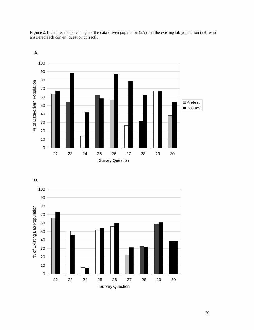
Figure 2. Illustrates the percentage of the data-driven population (2A) and the existing lab population (2B) who answered each content question correctly.

A.

0

10

20

30

40

50

60

70

80

90

100

22 23 24 25 26 27 28 29 30Survey Question

% o

f Dat

a-dr

iven

Pop

ulat

ion

PretestPosttest

B.

0

10

20

30

40

50

60

70

80

90

100

22 23 24 25 26 27 28 29 30Survey Question

% o

f Exi

stin

g La

b P

opul

atio

n

PretestPosttes

20

Figure 3. Illustrates the distribution of the percentage of the data-driven (3A) and existing lab (3B) populations as represented by their total content scores in the pretest and posttest.

A.

0

5

10

15

20

25

30

0 1 2 3 4 5 6 7 8 9

Total Score (out of 9)

% o

f Dat

a-dr

iven

Pop

ulat

ion

PRETESTPOSTTEST

B.

0

5

10

15

20

25

30

0 1 2 3 4 5 6 7 8 9

Total Score (out of 9)

% o

f Exi

stin

g La

b Po

pula

tion

PRETESTPOSTTEST

21

Qualitative data included observations of the classrooms. Students in the data-driven group had a mild frustration with vectors and having to make their own choices and interpretations. Some of the data-driven teaching assistants never really summed up student interpretations and conclusions, but all of them seemed to address individual groups' concerns about subjectivity and other aspects of the nature of science. Session II

Pretest student knowledge of the nature of science in both the data-driven and model-driven groups was comparable with the exception of questions 16 and 20 (science can study things from millions of years ago and scientists can come up with different but equally valid solutions to the same problem). The mean responses to these two questions were significantly different (p = 0.012 and p = 0.003 respectively, see Figures 4A and 4B). Within the model-driven population (pretest/posttest comparison), only questions 11 and 18 (science can prove anything, etc. and anything done scientifically can always be relied on to be accurate and reliable) did not show significant mean change (p > 0.05) between the pretest and posttest (Figures 4B and 4D). Table 6 summarizes the statistically significant mean changes. The data-driven population only showed significant change (p<0.01) for questions 12, 13, and 20 (involves uncertainties, requires creative activities, and different, but equally valid solutions). Mean response to these questions increased 3.86 to 4.70, 3.92 to 4.36, and 4.05 to 4.37, respectively (Figures 4A and 4C).

22

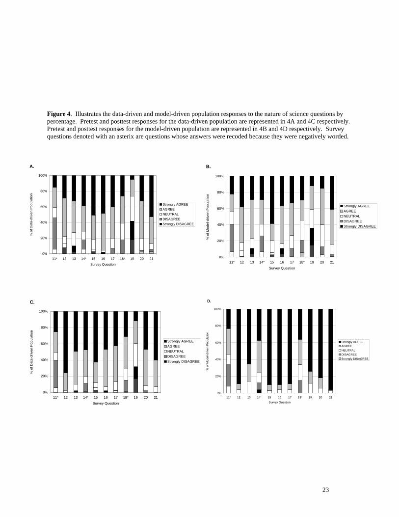
Figure 4. Illustrates the data-driven and model-driven population responses to the nature of science questions by percentage. Pretest and posttest responses for the data-driven population are represented in 4A and 4C respectively. Pretest and posttest responses for the model-driven population are represented in 4B and 4D respectively. Survey questions denoted with an asterix are questions whose answers were recoded because they were negatively worded.

B.

0%

20%

40%

60%

80%

100%

11* 12 13 14* 15 16 17 18* 19 20 21

Survey Question

% o

f Mod

el-d

riven

Pop

ulat

ion

Strongly AGREEAGREENEUTRALDISAGREEStrongly DISAGREE

A.

0%

20%

40%

60%

80%

100%

11* 12 13 14* 15 16 17 18* 19 20 21

Survey Question

% o

f Dat

a-dr

iven

Pop

ulat

ion

Strongly AGREEAGREENEUTRALDISAGREEStrongly DISAGREE

D.

0%

20%

40%

60%

80%

100%

11* 12 13 14* 15 16 17 18* 19 20 21

Survey Question

% o

f Mod

el-d

riven

Pop

ulat

ion

Strongly AGREEAGREENEUTRALDISAGREEStrongly DISAGREE

C.

0%

20%

40%

60%

80%

100%

11* 12 13 14* 15 16 17 18* 19 20 21

Survey Question

% o

f Dat

a-dr

iven

Pop

ulat

ion

Strongly AGREEAGREENEUTRALDISAGREEStrongly DISAGREE

23

Table 6. Model-driven population, Session II, Significant mean changes p=0.000. Question # Question Topic Pretest Mean Posttest Mean 12 uncertainties 4.11 4.85 13 creativity 3.90 4.52 14 changeability of science 3.55 3.96 15 can be done poorly 4.30 4.88 16 study things from millions of years ago 4.05 4.86 17 science is important for all people 3.93 4.85 19 subjectivity 3.03 4.62 20 different but equally valid solutions 3.60 4.77 21 disagreement is one of its strengths 4.19 4.93

24

Pretest content knowledge between the two groups was statistically different in their

pretest scores (p = 0.391). However, both groups showed a significant (p=0.000) positive shift from pretest to posttest in mean total score. The mean score of the model-driven group shifted from 3.67 to 6.19 (Figure 6B). The mean score of the data-driven group shifted from 3.92 to 6.11 (Figure 6A). When the content questions were examined individually for the model-driven group, 5 out of the 9 questions showed remarkable increases in the number of, and therefore the percentage, of students who answered the questions correctly (Figure 5B). Changes in percentage of population were considered remarkable if they changed by an additional 20%. When the content questions were examined individually for the data-driven group, only 4 out of the 9 questions showed remarkable increases. However, two questions, showed just under an additional 20% of the population (Figure 5A).

25

Figure 5. Illustrates the percentage of the data-driven population (5A) and the model-driven population (5B) who answered each content question correctly.

A.

0102030405060708090

100

22 23 24 25 26 27 28 29 30

Survey Question

% o

f Mod

el-d

riven

Pop

ulat

ion

PretestPosttest

B.

0102030405060708090

100

22 23 24 25 26 27 28 29 30Survey Question

% o

f Mod

el-d

riven

Pop

ulat

ion

PretestPosttest

26

Figure 6. Illustrates the distribution of the percentage of the data-driven (6A) and model-driven (6B) populations as represented by their total content scores in the pretest and posttest.

A.

0

5

10

15

20

25

30

35

0 1 2 3 4 5 6 7 8 9

Total Score (out of 9)

% o

f Dat

a-dr

iven

Pop

ulat

ion

PRETESTPOSTTEST

B.

0

5

10

15

20

25

30

35

0 1 2 3 4 5 6 7 8 9

Total Score (out of 9)

% o

f Mod

el-d

riven

Pop

ulat

ion

PRETESTPOSTTEST

27

Qualitative results included both class observations and written questionnaire responses by the students. First, students in the data-driven group were mildly frustrated in the beginning with the subjectivity of picking data points and having to make their own choices, but they quickly adjusted to having to make reasonable decisions and propose models and solutions. Second, students in the model-driven group were easily frustrated when they were working on a part of the exercise that was not "plug and chug." This frustration transformed into open hostility towards the teaching assistant when at one point in the lab they were forced to make a choice about where to make a measurement. Third, in general, students in the data-driven group worked with their teaching assistants to come to some reasonable conclusion at several points in the lab. In particular, they would listen to teaching assistants' explanations, but not necessarily accept it or write it down immediately. The model-driven group, on the other hand, appeared to view their teaching assistants as their answer source. They constantly asked if they were doing it right. When the teaching assistants explained something or talked about the nature of science (when the measurement of the mountains brought it up), the students would write the teaching assistants' response down immediately "as correct," without reflecting on it themselves.

Student responses to the questionnaire at the end of the exercises indicated that the majority of students in both groups felt that the data in their lab exercises were realistic (85.1% of the data-driven group and 70.0% of the model-driven group). Responses from both the model-driven and data-driven groups also indicated that the students gained in understanding that science is not always accurate, can contain errors, is subjective, and involves many uncertainties. Overall, the comments on the questionnaires did not speak to any other aspects of content knowledge or methods of science. However, almost all of the students in each group commented on the difficulty of calculating, drawing, and using vectors.

28

Discussion Session I

We considered ANOVA to be a valid test for significance, despite some skewness of the distributions, because the largest variance was not four or more times greater than the smallest variance for the distributions being compared (Howell, 1997). Skewness values for the distributions also, with a few exceptions, fell between -1 and +1, which is generally acceptable. Additionally, the results of the significance tests make sense upon inspection of the data. Those questions, which were found to be statistically significantly different, are also strikingly different in their graphical representation.

Because the existing lab showed no significant change in content knowledge and the nature of science (overall), it is reasonable to use the group as a proxy control group. And since the pretest scores of the existing lab group are statistically similar to the posttest scores of the existing lab group, we can infer that apparent testing effect has been minimized in our experiment. We were pleasantly surprised to learn that the majority of students came into the experiment with a solid understanding of the nature of science, as evidenced by the dominance of agree and strongly agree responses. It seems unlikely, therefore, that we would observe dramatic changes in student understanding of the nature of science. What we observed instead was a more subtle change from agree to strongly agree (look at the response to questions 12, 14, and 20 in Figures 1A and 1C).

While the changes in student understanding of the nature of science was not as dramatic as we had anticipated, positive change was still recorded, indicating that working with a data-driven approach with real data does have a positive influence on student understanding of the nature of science. The notable mean shift in student content knowledge also indicates that a data-driven approach with real data is effective at conveying content material. Observations of the students working on this lab seemed to support these conclusions. Session II Despite the statistically significant difference between the model-driven and data-driven groups in the pretest, they both showed reasonably comparable increases in mean total content knowledge scores (2.19 for data-driven and 2.52 for model-driven). It seems reasonable, therefore, to conclude that both approaches were approximately equally effective at conveying content material to students. It is important to remember that the significance test does not exclude the possibility that they are comparable. As illustrated in Figures 4A and B, the model-driven approach was clearly more effective at conveying the nature of science to students than the data-driven approach. We suggest that this dramatic change results from the pre-existing model-driven mindset that students enter into when they are taught with a model-driven approach. Students misinterpret models as facts because the models are presented up front as being "accepted truths." When students are presented with a concept, such as "science deals with many uncertainties," while they are in this mode of "what is said is true," they more readily accept it as true. The teacher is all-knowing and responsible for disseminating knowledge in the model-driven approach. Additionally, if students are at a developmental stage where they see science as having absolute truths (Magolda, 1992), they are more likely to trust and accept the teacher's authority and opinion over their own.

This also explains why students in the data-driven approach group did not gain as much in their understanding of the nature of science. Students are responsible for gaining knowledge through their own logic in the data-driven approach. They are not reliant on the teacher, and thus

29

they do not accept the teacher's opinions or comments on the nature of science as readily as do those with a model-driven mindset. The observations of students made during the labs support this. Students in the data-driven group questioned the nature of science and the science they were doing throughout the lab. They would ask the teacher what he thought, but they didn't immediately accept it and write it down, as those in the model-driven group did. Though mildly resistant at first, it appeared that the data-driven students entered into a mindset in which they accepted their role in creating models, interpreting the data, and drawing their own conclusions. The model-driven students, on the other hand, were focused on the teacher's interpretation of the data and conclusions. They repeatedly demanded to know what the teacher wanted them know.

When we look at the dramatic increase in correct responses to the nature of science questions in the model-driven group, it is important to reflect on what the geoscience education community wants students to be able to do with the nature of science. Do we just want them to be able to parrot the correct responses when they are asked about the nature of science? By testing students this way, we aren't assessing whether or not they can use what they know about the nature of science to think critically about science. They may be able to tell us that science can done poorly, but may not be able to look at a study and assess its worth based on whether it was done poorly or not. We recommend that future studies include a component that assesses student ability to apply these aspects of the nature of science. While we feel that this is an important issue that needs to be investigated further, we also need to address the shortcomings of the study. We believe that the comparison between approaches was validly accomplished in the experimental labs. However, we feel that the contrived nature of the data in the model-driven lab was somewhat compromised. One measurement, out of many measurements and calculations the students did in the lab, became "real" for the students. They were not given an exact location on a map to measure the width of a mountain range. Instead, they had to decide for themselves where to measure (see Treatment C in the Methods section). As noted in the classroom observations, this resulted in widespread frustration (more so than the same measurement in the data-driven group). Discussion then ensued about subjectivity.

While we believe that this potentially skewed some of the nature of science posttest results in the model-driven group, we don't believe that its significance is so great that it accounts for all of the observed change, because if this were the case, results should have been comparable with the data-driven group that openly dealt with subjectivity. Also, when one considers that the majority of the students in the model-driven approach thought that, according to their questionnaire comments, the data were realistic despite being told explicitly that the data were modified to work out better, it is apparent that some other factor is resulting in the dramatic difference between the groups. These students believed the parts in which their measurements were contrived (so that they concluded with specific answers) were indeed real. When they had to make a choice about which number to use, they didn't consider any of their choices to be valid (based on classroom observation). Instead, they demanded that the teaching assistant tell them which value or measuring point was "right." As noted by our observations, students in the data-driven group that had to make choices from the beginning did not have this openly hostile reaction to this part of the lab. Instead, they acknowledge the subjectivity of their choices, but accepted them as reasonable. We suspect that the two approaches evoke different attitudes in the students, which in turn impacts what they get out of the exercise.

Despite the apparent effectiveness of the model-driven approach as indicated by the quantitative assessment data, we believe that based on the qualitative assessment data, the data-

30

driven approach may be more effective than the model-driven approach. The quantitatively observed changes in students' understanding of the concepts surveyed, such as uncertainty, creativity, different, but equally valid results, and poor science combined with the observation of students transitioning into a more independent role in the lab experience indicate that the data-driven approach has the potential to be more effective than the model-driven approach. Students have to struggle more in a data-driven exercise, as they are constantly required to reflect on what they are doing and how they did it. Students in our data-driven group were observed to have the most difficulty with these parts of the exercise. Therefore it seems logical that they would need to be exposed to this approach consistently during a course to get more out of it. It is difficult to switch from always being told how the Earth works and why it works that way, to having to figure out how the Earth works from uncertain, "messy" data.

Despite these challenges, students working through the data-driven lab exercises adjusted more successfully to thinking on their own than did their model-driven counterparts. Students in the data-driven group did not develop openly hostile reactions to having to think on their own, presumably because they were forced to think on their own constantly throughout the lab exercise and were repeatedly asked by their teacher what they thought and why. Observing the data-driven students openly embracing independent thinking by the end of the exercise indicates that they became more accepting of the contextual nature of scientific methodology. Observation and study of a longer term project than this one would elucidate to what degree that data-driven approach may be more effective in communicating the nature and methods of science.

31

Implications The results do not speak to any radical changes in the way teachers are using data

resources in their classrooms, but they do indicate an apparent difference in the approaches to using data in short, one time assignment formats. Teachers need to be aware that just because they are using real data doesn't mean the assignment will be more effective at conveying content knowledge and/or nature of science concepts, or that it will seem more real to students. Further study needs to be done to determine the effectiveness of a more long-term timeframe when using datasets, specifically with these two different approaches. Perhaps over a longer time scale, the data-driven exercises would be more effective than the model-driven exercises, as it would allow the students more time to adjust to the role that data plays in scientific endeavors.

Studies addressing these issues are especially important as the education community transitions from a paper-based to a computer-based electronic community. Organizations, such as the DLESE, National Science Digital Library (NSDL), and Earthscope, to name a few, are providing data-rich resources and making them readily available to teachers online. As teachers are encouraged to use the resources provided by these web-based clearinghouses, it is important that they also be given researched guidelines for effectively implementing these data in the classroom. Investigating the effectiveness of these resources is in fact one of the stated goals of DLESE (DLESE, 2001). We hope that this study will encourage future studies of data-rich experiences in the classroom. We believe that these two approaches and their commonly associated data types are different enough that they will vary in their effectiveness at conveying both content knowledge and the nature of science to students. We hope, therefore, that the results of our study will help DLESE constrain its definition of a data-rich experience, which currently includes the spectrum of these end member approaches and their commonly associated data types.

32

References Abd-El-Khalick, F., Bell, R., & Lederman, N., 1998, The nature of science and instructional

practice: making the unnatural natural, Science Education, vol. 82, p. 417-436. Alters, B., 1997, Whose nature of science? Journal of Research in Science Teaching, vol. 34, n.

1, p. 39-55. Alters, B., 1997, Nature of science: a diversity or uniformity of ideas? Journal of Research in

Science Teaching, vol. 34, n. 10, p. 1105-1108. Akerson, V., & Abd-El-Khalick, F., 2003, Teaching elements of nature of science: A yearlong

case study of a fourth-grade teacher, Journal of Research in Science Teaching, vol. 40, n. 10, p. 1025-1049.

Bell, R., Blair, L., Crawford, B., & Lederman, N., 2003, Just do it? impact of a science

apprenticeship program on high school students' understandings of the nature of science and scientific inquiry, Journal of Research in Science Teaching, vol. 40, n. 5, p. 487-509.

Bell, R., Lederman, N., & Abd-El-Khalick, F., 2000, Developing and acting upon one's

conception of the nature of science: a follow-up study, Journal of Research in Science Teaching, vol. 37, n. 6, p. 563-581.

Bianchini, J., & Colburn, A., 2000, Teaching the nature of science through inquiry to prospective

elementary teachers: a tale of two researchers, Journal of Research in Science Teaching, vol. 37, n. 2, p. 177-209.

Busch, R., editor, 2003, Laboratory Manual in Physical Geology (6th edition), New Jersey,

Prentice Hall, 271 p. Collier, M., 1999, A Land in Motion, Los Angeles, CA, University of California Press, 118 p. DLESE, History of DLESE (discussing link to NSF/Geoscience Directorate),

http://www.dlese.org/about/history.html#geo (17 April, 2004).

DLESE, October 2001, Strategic Plan, Version 12.0, http://www.dlese.org/documents/plans/stratplanver12.html (17 April, 2004).

DLESE, 2003?, Using data in the classroom,

http://www.dlesecommunity.carleton.edu/research_education/usingdata/index.html (17 April, 2004).

Dhingra, K., 2003, Thinking about television science: How students understand the nature of

science from different program genres, Journal of Research in Science Teaching, vol. 40, n. 2, p. 234-256.

33

Flammer, L., 1997, Evolution and Nature of Science Institutes Publication (ENSIWeb):

Teaching the nature of science: science knowledge survey, http://www.indiana.edu/~ensiweb/lessons/unt.n.s.html (17 April, 2004).

Gall, M., Gall, J., & Borg, W., 2003, Educational Research (7th edition), White Plains, NY,

Longman Publishers, p. 365-430. Gordon, R., 1998, Balancing real-world problems with real-world results, Phi Delta Kappan, p.

390-393. Howell, D. C., 1997, Statistical methods for psychology (4th Edition), University of Vermont:

Duxbury Press, p. 321-322. Lederman, N., 1992, Students’ and teachers’ conceptions of the nature of science: a review of the

research, Journal of Research in Science Teaching, vol. 29, n. 4, p. 331-359. Lederman, N., Abd-El-Khalick, F., Bell, R., & Schwartz, R., 2002, Views of nature of science

questionnaire: toward valid and meaningful assessment of learners' conceptions of nature of science, Journal of Research in Science Teaching, vol. 39, n. 6, p. 497-521.

Lederman, N. & Druger, M., 1985, Classroom factors related to changes in students’ conceptions

of the nature of science, Journal of Research in Science Teaching, vol. 22, n. 7, p. 649-662.

Lederman, N., & O’Malley, M., 1990, Students’ perceptions of tentativeness in science:

development, use, and sources of change, Science Education, vol. 74, n. 2, p. 225-239. Lederman, N., & Zeidler, D., 1987, Science teachers conceptions of the nature of science: do

they really influence behavior? Science Education, vol. 71, n. 5, p. 721-734. Lewis Center for Educational Research, Science knowledge survey,

www.lewiscenter.org/force/1070/subprojects/Instructor/IPB10%20Main%20Page/IPB10%201st%20Quarter/SciKnowSur.prn.pdf (July 2003).

Magolda, M. B., 1992, Knowing and Reasoning in College. U.S., Jossey-Bass Publishing, p.

139. Matthews, M., 1998, In defense of modest goals when teaching about the nature of science,

Journal of Research in Science Teaching, vol. 35, n. 2, p. 161-174. National Research Council, 1996, National Science Education Standards, Ch. 6 Science Content,

http://www.nap.edu/readingroom/books/nses/6a.html#pslsesss (22 April, 2004).

34

Osborne, J., Collins, S., Ratcliffe, M., Millar, R. & Duschl, R., 2003, What ideas-about-science should be taught in school science? A Delphi study of the expert community, Journal of Research in Science Teaching, vol. 40, n. 7, p. 692-720.

Palmquist, B. & Finley, F., 1998, A response to Bell, Lederman, and Abd-El-Khalick’s explicit

comments, Journal of Research in Science Teaching, vol. 35, n. 9, p. 1063-1064. Palmquist, B. & Finley, F., 1997, Preservice teachers’ views of the nature of science during a

postbaccalaureate science teaching program, Journal of Research in Science Teaching, vol. 34, n. 6, p. 595-615.

Pomeroy, D., 1993, Implications of teachers’ beliefs about the nature of science: comparison of

the beliefs of scientists, secondary science teachers, and elementary teachers, Science Education, vol. 77, n. 3, p. 261-278.

Schwartz, R., & Lederman, N., 2002, It's the nature of the beast : The influence of knowledge

and intentions on learning and teaching nature of science, Journal of Research in Science Teaching, vol. 39, n. 3, p. 205-236.

Sieh, K.E., and Jahns, R.H., 1984, Holcene activity of the San Andreas Fault at Wallace Creek,

California: Geological Society of America Bulletin, v. 95, p. 883-896. Sieh, K. E., and Wallace, R. E., 1987, The San Andreas fault at Wallace Creek, San Luis Obispo

County, California: Geological Society of America Centennial Field Guide--Cordilleran Section, p. 233-238.

Smith, M., Lederman, N., Bell, R., McComas, W., & Clough, M., 1997, How great is the

disagreement about the nature of science: a response to Alters, Journal of Research in Science Teaching, vol. 34, n. 10, p. 1101-1103.

Somerville, R., 1996?, NSF GEO Report: Geoscience Education: A Recommend Strategy

(section entitled “Research on Geoscience Education”) http://www.geo.nsf.gov/adgeo/geoedu/97_171.htm (17 April, 2004).

Spotila, J., House, M., Blythe, A., Niemi, N., & Bank, G., 2002, Controls on the erosion and

geomorphic evolution of the San Bernardino and San Gabriel mountains, southern California. Geological Society of America Special Paper, vol. 365, p. 205-230.

Stewart, J. & Rudolph, J., 2001, Considering the nature of scientific problems when designing

science curricula, Science Education, vol. 85, p. 207-222. Uyeda, S., Madden, J., Brigham, L., Luft, J., and Washburne, J., 2002, Solving authentic science

problems, The Science Teacher, p. 24-29.

35

List of Appendices Appendix A: Survey Instrument Appendix B: Observation sheet Appendix C: Student Questionnaire (used in Session II) Appendix D: Data-driven lab exercise (Session II) Appendix E: Model-driven lab exercise (Session II) Appendix F: Summary of student questionnaire responses (Session II) Appendix G: Summary of statistical results (Sessions I & II)

36

Appendix A: Survey instrument [ ] indicate additions made for Session II (only the nature of science questions were affected). Student Survey This survey consists of three parts (background, understanding of the nature of science, and content knowledge) with 30 questions in total. Please answer all the questions honestly. Thank you for your time and effort! INSTRUCTIONS: Write and fill in the corresponding bubbles for your student ID number on the top of the OPSCAN form. Answer the following question on your OPSCAN sheet. Part I: Background Read each statement and complete it with the choice that best fits. Fill in the corresponding bubble on the opscan answer sheet. _______1. I am: 1. Male 2. Female _______2. My class standing is: 1. freshman 2. sophomore 3. junior 4. senior 5. other _______3. My GPA falls in the following range: 1. 4.0-3.7 2. 3.6-2.7 3. 2.6-1.7 4. 1.6-0.0 _______4. My major program of study is part of the following college: 1. Agriculture and Life Sciences 2. Architecture and Urban Studies 3. Business 4. Engineering 5. Liberal Arts and Human Sciences 6. Natural Resources 7. Science 8. University Studies 9. Veterinary Medicine _______5. I describe my ethnic group/race as: 1. African American 2. Asian 3. Hispanic

37

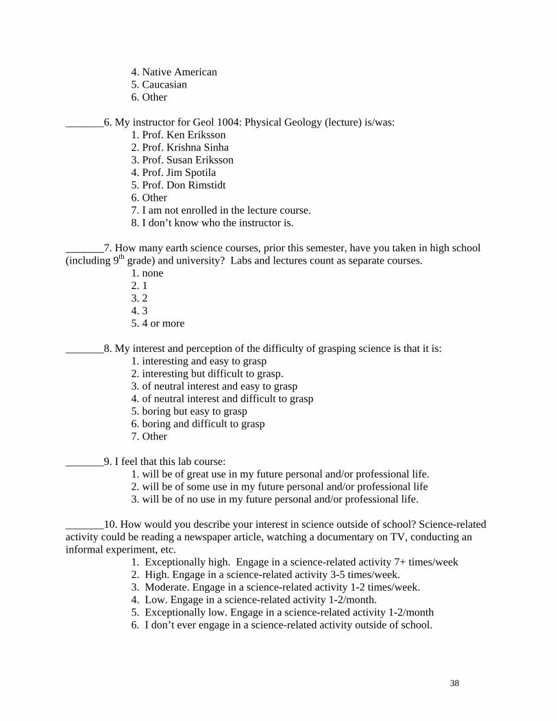
4. Native American 5. Caucasian 6. Other _______6. My instructor for Geol 1004: Physical Geology (lecture) is/was: 1. Prof. Ken Eriksson 2. Prof. Krishna Sinha 3. Prof. Susan Eriksson 4. Prof. Jim Spotila 5. Prof. Don Rimstidt 6. Other 7. I am not enrolled in the lecture course. 8. I don’t know who the instructor is. _______7. How many earth science courses, prior this semester, have you taken in high school (including 9th grade) and university? Labs and lectures count as separate courses. 1. none 2. 1 3. 2 4. 3 5. 4 or more _______8. My interest and perception of the difficulty of grasping science is that it is: 1. interesting and easy to grasp 2. interesting but difficult to grasp. 3. of neutral interest and easy to grasp

4. of neutral interest and difficult to grasp 5. boring but easy to grasp 6. boring and difficult to grasp 7. Other

_______9. I feel that this lab course: 1. will be of great use in my future personal and/or professional life. 2. will be of some use in my future personal and/or professional life 3. will be of no use in my future personal and/or professional life. _______10. How would you describe your interest in science outside of school? Science-related activity could be reading a newspaper article, watching a documentary on TV, conducting an informal experiment, etc. 1. Exceptionally high. Engage in a science-related activity 7+ times/week 2. High. Engage in a science-related activity 3-5 times/week. 3. Moderate. Engage in a science-related activity 1-2 times/week. 4. Low. Engage in a science-related activity 1-2/month. 5. Exceptionally low. Engage in a science-related activity 1-2/month 6. I don’t ever engage in a science-related activity outside of school.

38

Part II: The Nature of Science Read each statement and decide the extent to which you agree or disagree with the statement. Fill in the corresponding bubble on the opscan answer sheet. Source: www.lewiscenter.org _______11. Science can prove anything, solve any problem, or answer any question.

1. Strongly disagree 2. Somewhat disagree 3. Neutral 4. Somewhat agree 5. Strongly agree

_______12. Science involves dealing with many uncertainties.

1. Strongly disagree 2. Somewhat disagree 3. Neutral 4. Somewhat agree 5. Strongly agree

_______13. Science requires creative activity, [such as creating models for how something works.]

1. Strongly disagree 2. Somewhat disagree 3. Neutral 4. Somewhat agree 5. Strongly agree

_______14. Something that is “proven scientifically” is considered by scientists as being a fact, and therefore no longer subject to change.

1. Strongly disagree 2. Somewhat disagree 3. Neutral 4. Somewhat agree 5. Strongly agree

_______15. Science can be done poorly.

1. Strongly disagree 2. Somewhat disagree 3. Neutral 4. Somewhat agree 5. Strongly agree

_______16. Science can study things and events from millions of years ago.

1. Strongly disagree

39

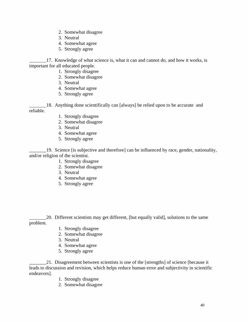
2. Somewhat disagree 3. Neutral 4. Somewhat agree 5. Strongly agree

_______17. Knowledge of what science is, what it can and cannot do, and how it works, is important for all educated people.

1. Strongly disagree 2. Somewhat disagree 3. Neutral 4. Somewhat agree 5. Strongly agree

_______18. Anything done scientifically can [always] be relied upon to be accurate and reliable.

1. Strongly disagree 2. Somewhat disagree 3. Neutral 4. Somewhat agree 5. Strongly agree

_______19. Science [is subjective and therefore] can be influenced by race, gender, nationality, and/or religion of the scientist.

1. Strongly disagree 2. Somewhat disagree 3. Neutral 4. Somewhat agree 5. Strongly agree

_______20. Different scientists may get different, [but equally valid], solutions to the same problem.

1. Strongly disagree 2. Somewhat disagree 3. Neutral 4. Somewhat agree 5. Strongly agree

_______21. Disagreement between scientists is one of the [strengths] of science [because it leads to discussion and revision, which helps reduce human error and subjectivity in scientific endeavors].

1. Strongly disagree 2. Somewhat disagree

40

3. Neutral 4. Somewhat agree 5. Strongly agree

Part III: Content Knowledge Read each statement. Based on your knowledge of geology, decide if you agree or disagree with it, or don’t know enough about it to make a decision. _______22. Scientists can directly measure movement along a strike-slip fault. 1. Agree 2. Disagree 3. I don’t know. _______23. The plate motion associated with transform plate boundaries can uplift mountains. 1. Agree 2. Disagree 3. I don’t know. _______24. (U-Th)/He dating can be used for determining when a rock formed. 1. Agree 2. Disagree 3. I don’t know. _______25. Plate boundaries are always parallel to plate motion. 1. Agree 2. Disagree 3. I don’t know. _______26. A vector has direction but no magnitude. 1. Agree 2. Disagree 3. I don’t know. _______27. He is a by-product of the radioactive decay of U into Th. 1. Agree 2. Disagree 3. I don’t know. _______28. The entire length of the San Andreas fault zone is oriented in the same direction. 1. Agree 2. Disagree 3. I don’t know.

41

_______29. If a plate is said to be moving at an average rate of 50mm/yr, that means that the plate moved 50mm last year. 1. Agree 2. Disagree 3. I don’t know. _______30. Scientists cannot directly measure the uplift of mountains. 1. Agree 2. Disagree 3. I don’t know.

42

Appendix B: Observation Sheet TA code: _________ Student interest in content: _____majority _____about half _____less than half _____only a few _____no one Student comprehension about what to do: _____majority _____about half _____less than half _____only a few _____no one Student participation in class discussions: _____majority _____about half _____less than half _____only a few _____no one Student attention during mini-lectures: _____majority _____about half _____less than half _____only a few _____no one Student attitude towards TA: Group/Table Dynamics: _____everyone working through problems _____about half

_____one or two doing the work, others copying

TA attitude towards students:

43

TA attitude about course/content: ** How clearly teaching assistants explained content and how they dealt with the nature of science issues was also recorded, as well as student comments.

44

Appendix C: Student Questionnaire (used in Session II)* *Students were given more space between questions for their answers.

What did you think of the new lab? List everything you feel that you learned from this lab: List everything that you feel you learned about science and scientific research in general from this lab: Describe any parts that you found frustrating (what did they ask you to do and why was it frustrating)? Describe any parts/activities of the lab that you feel contained confusing instructions: For the next questions, Circle your response and make any comments you wish: Did you come away from this lab with a greater appreciation for the complexity and difficulty of measuring relative plate motions?

Yes No Other:__________ Did you come away from this lab with a greater understanding of the uncertainties and subjectivity that geoscientists struggle with when modeling how the world works?

Yes No Other:__________

Do you feel that the data you used was realistic and represented actual data from a formal geological study?

Yes No Other:__________

45

Overall, did you feel like you understood where the lab was going and what you needed to do?

Yes No Other:__________ Overall, how did this lab compare to the labs you've done up until this point in the course?

46

Appendix D: Data-driven lab exercise (Session II)

Lab 10: Applying Geologic Methods to Real Issues Up to now, most of your effort in this course has been to observe and record information and then to use this information to make interpretations. In this lab, you will have an opportunity to use these skills by tackling a real and ongoing geoscientific research problem using real data. You will be able to see how geoscientists struggle with these data in formulating ideas (models) that help us appreciate how the world might work. These models that we create are hypotheses and they are dynamic—always undergoing revision to better fit the ever-increasing data that we collect. It is through this iterative process of carefully observing the world around us, interpreting our observations using scientific reasoning and openly communicating with other scientists that we progress with our ideas. In this lab, we’ll examine how this is done in an ongoing research project in our department here at Tech. Keep in mind though that as with any scientific investigation, you might also end up with more questions. Don’t expect answers all of the time or even most of the time—science doesn’t always yield answers. Part l: The Nature of the Geosciences Personal Viewpoint: Now that you have had this opportunity to study the Earth from the observation and record-keeping perspective of a geoscientist, what do you think about the “nature of the geosciences”? Please take a few thoughtful minutes to reflect on the following questions: How do you define science? (Science is the study of…) Aside from the obvious content differences between the different branches of science, do the methods that geoscientists use differ from those used in the other sciences? If yes or no, please elaborate on how the different branches of science do/don’t differ in the methods that each one uses. Remember, methods are “how” scientists go about doing things. During this laboratory course, you have been introduced to one of the most powerful tools that we use to study the Earth—that of careful observation. You have also reasoned through these lab exercises deductively or empirically (an event can be explained by an immediately preceding event). Science can only address questions using this form of reasoning. Now, in this lab, you

47

will have the opportunity to tackle a real geoscientific research problem. It is through these types of problems that we gain in our appreciation of the types of questions that science can and can’t answer. Part ll: The San Andreas Fault: A Big Rip in our Continent TA Presentation and Discussion: Let’s begin a trip together to look at one of the most active fault regions in North America—the San Andreas Fault System. If you could know any one thing about the San Andreas Fault, I’ll bet you would want to know when and where the next “big one” would occur. So would most geoscientists and probably most of the population of California! While we can’t “know” when this will happen, we can estimate the likelihood of a large quake occurring based on the amount of strain being stored in the rocks adjacent to the fault and our model for how that strain will be released. This stored potential energy can be estimated in part by studying the rate of motion of the two plates that rub shoulders along this transform boundary—the Pacific Plate and the North American Plate. When you think about it this way, calculating these rates and directions of motion becomes far more than an exercise in curiosity—it becomes a necessity for helping us understand how much strain a fault can store before it lets go causing a potentially devastating earthquake. How do scientists calculate plate motions? What models do geologists use to calculate plate motions? If you think about this problem for long, you begin to realize that all plates are moving at different rates and in different directions. Nowhere are they “fixed” relative to a global frame of reference such as the axis of rotation of the globe. The best we can do is to measure relative plate motion between plates and their spreading centers. By determining this relative motion, we can determine rates of slip along other plate boundaries such as along the San Andreas Fault. Thought Exercise: We need to know how fast and in what direction plates move away from a mid-ocean ridge. What data would you need in order to calculate the rate of movement and the relative motion of the two plates that are being formed along a mid-ocean ridge? As you may recall from lecture, the Earth's magnetic field periodically reverses polarity. Such episodes occur relatively rapidly over perhaps a few hundred to a thousand years. As magma erupts from the mid-ocean spreading centers, it cools quickly to form basaltic oceanic crust. Magnetic materials within the cooling lava align with the earth’s magnetic field and become “frozen” in that orientation. When the poles reverse, rocks that cool after the reversal become magnetized in the opposite orientation. This process has produced magnetic “stripes” in the ocean floor. The boundary that separates rocks magnetized in one orientation from those of

48

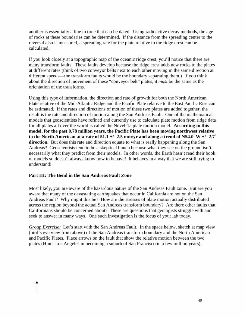
another is essentially a line in time that can be dated. Using radioactive decay methods, the age of rocks at these boundaries can be determined. If the distance from the spreading center to the reversal also is measured, a spreading rate for the plate relative to the ridge crest can be calculated. If you look closely at a topographic map of the oceanic ridge crest, you’ll notice that there are many transform faults. These faults develop because the ridge crest adds new rocks to the plates at different rates (think of two conveyor belts next to each other moving in the same direction at different speeds—the transform faults would be the boundary separating them.) If you think about the direction of movement of these “conveyor belt” plates, it must be the same as the orientation of the transforms. Using this type of information, the direction and rate of growth for both the North American Plate relative of the Mid-Atlantic Ridge and the Pacific Plate relative to the East Pacific Rise can be estimated. If the rates and directions of motion of these two plates are added together, the result is the rate and direction of motion along the San Andreas Fault. One of the mathematical models that geoscientists have refined and currently use to calculate plate motion from ridge data for all plates all over the world is called the Nuvel-1a plate motion model. According to this model, for the past 0.78 million years, the Pacific Plate has been moving northwest relative to the North American at a rate of 51.1 +/- 2.5 mm/yr and along a trend of N54.0• W +/- 2.7•

direction. But does this rate and direction equate to what is really happening along the San Andreas? Geoscientists tend to be a skeptical bunch because what they see on the ground isn’t necessarily what they predict from their models. In other words, the Earth hasn’t read their book of models so doesn’t always know how to behave! It behaves in a way that we are still trying to understand! Part III: The Bend in the San Andreas Fault Zone Most likely, you are aware of the hazardous nature of the San Andreas Fault zone. But are you aware that many of the devastating earthquakes that occur in California are not on the San Andreas Fault? Why might this be? How are the stresses of plate motion actually distributed across the region beyond the actual San Andreas transform boundary? Are there other faults that Californians should be concerned about? These are questions that geologists struggle with and seek to answer in many ways. One such investigation is the focus of your lab today. Group Exercise: Let’s start with the San Andreas Fault. In the space below, sketch at map view (bird’s eye view from above) of the San Andreas transform boundary and the North American and Pacific Plates. Place arrows on the fault that show the relative motion between the two plates (Hint: Los Angeles in becoming a suburb of San Francisco in a few million years).

49

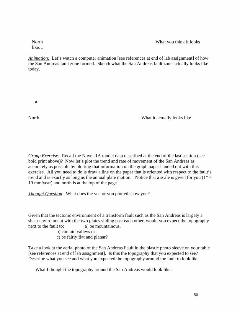
North What you think it looks like…

Animation: Let’s watch a computer animation [see references at end of lab assignment] of how the San Andreas fault zone formed. Sketch what the San Andreas fault zone actually looks like today. North What it actually looks like… Group Exercise: Recall the Nuvel-1A model data described at the end of the last section (see bold print above)? Now let’s plot the trend and rate of movement of the San Andreas as accurately as possible by plotting that information on the graph paper handed out with this exercise. All you need to do is draw a line on the paper that is oriented with respect to the fault’s trend and is exactly as long as the annual plate motion. Notice that a scale is given for you (1” = 10 mm/year) and north is at the top of the page. Thought Question: What does the vector you plotted show you? Given that the tectonic environment of a transform fault such as the San Andreas is largely a shear environment with the two plates sliding past each other, would you expect the topography next to the fault to: a) be mountainous,

b) contain valleys or c) be fairly flat and planar?

Take a look at the aerial photo of the San Andreas Fault in the plastic photo sleeve on your table [see references at end of lab assignment]. Is this the topography that you expected to see? Describe what you see and what you expected the topography around the fault to look like.

What I thought the topography around the San Andreas would look like:

50

What the topography around the San Andreas actually looks like:

Is there a discrepancy here? If yes, could our simple transform/shearing model of how the fault “is supposed to work” be incomplete? If you feel there is a disconnect between the model you have learned that describes how transform faults look and work and what you actually see in the photo, you’ve observed what many skeptical geoscientists have observed. The fault just isn’t behaving properly in this area! Turn over your photo sleeve to look at the tectonic map of North America [see references at end of lab assignment]. This photo was taken along the San Andreas Fault to the southwest of the “R” in “SAN ANDREAS FAULT” on the map. Group Exercise: Can you imagine how the crust and surface rocks near a bend in a transform fault accommodate strike-slip plate motion? How might movement along the fault affect topography near the bend? To get an idea, use the pieces of cut felt on your table to model movement on the fault. Orient the felt such that the fault is trending northwest. Slowly and very slightly drag the left-hand piece of felt toward the northwest. (This motion replicates the right-lateral motion on the San Andreas Fault.) How does the topography change near the bend in the fault? As you play with the felt, there will probably be several possible geometries of folds and uplifts that develop. Based on your observations of how the felt accommodates this motion, create/sketch a revised block model for how the San Andreas behaves tectonically. What about the fault/plate boundary causes this uplift in felt to occur? Group/Class Exercise: Your observations of how the crust behaves combined with your interpretation of these observations form a descriptive model (a hypothesis) of how the surface and shallow crust might accommodate motion along the San Andreas at the bend. Think this through and describe this model carefully because this is what you will test in the remainder of this exercise. Describe how the upper crust might be accommodating plate motion near the bend in the San Andreas Fault based on your block model above. Use the following terms in your

51

description: strike slip motion, convergence, orientation of the plate boundary, and orientation of the plate motion. The descriptive model (an idea) that you have just formulated should explain why the San Andreas Fault zone is mountainous along the bend in the fault just north of Los Angeles. As you have discovered through this simple exercise, it is the bend that results in a component of convergence. This compressive stress from convergence has lifted the rocks up forming mountains (the San Gabriel and San Bernardino Mountains rise to 10,000 feet above the Los Angeles basin showing that this is indeed a significant process). The term that geoscientists apply to the stress that compresses rocks across a bend in a transform fault is called transpression. Thought Question: If instead of deviating to the west, the bend had deviated to the east instead. To model this with your felt, turn it over such that the felt is oriented to the northeast and move the felt right-laterally. Can you describe or sketch the kind of structure that would form? Interestingly, there is a structure like this to the southeast of the San Andreas bend that we have been studying. Death Valley is the lowest point in North America and it is, in part, a “pull-apart” basin. Death Valley has formed along another right-lateral strike-slip fault zone, the Eastern California Shear Zone that bends easterly. Movement along the bend in this transform-type shear zone has resulted in tensional (pull-apart) instead of compressional stresses. Geoscientists refer to this stress environment as transtensional. Part IV: Determining Rates of Slip along the San Andreas Fault Now that we have an idea (a descriptive model or hypothesis) about how the crust behaves near the bend in the San Andreas, we can test our hypothesis by examining the offset rates in the vicinity of the bend to see whether these rates “add up” to equal the movement along the San Andreas Fault determined by the Nuvel-1a model. Thought Question: If the rate and direction of offset that we measure equals the NUVEL-1A data for total plate motion, what does that tell us about our revised model (the one you sketched and described in Part III)?

52

Group/Class Exercise: How might you determine the rate of slip along a transform fault such as the San Andreas? Think of at least two types of information that you would need to know and the kinds of features that might provide it.

Information needed: Features that might provide this information:

Sketch a block diagram showing how you would calculate the rate of slip on a transform fault: If you said you needed to find features that have been offset by the fault that also can be reliably dated, you’re on the right track. Features such as rocks, stream drainages, even mineral deposits are offset along the length of the San Andreas. The trick is getting an age on that feature that reliably indicates when it was last connected across the fault. So, if you know how long ago the feature was last connected across the fault and then if you measure the distance that now separates it, you can estimate an average rate of slip along the fault in that location. So let’s try estimating the rate at which the Pacific plate is moving northwest relative to the North American plate along a portion of the San Andreas in the Carrizo Plain area just north of the bend. We’ll look at the Wallace Creek drainage (see the topographic map of Wallace Creek in the photo sleeve on your table) [see references at end of lab assignment]. Notice that Wallace Creek drains across the San Andreas Fault from northeast to southwest. Its downstream portion has been offset periodically by the fault. During the late 1970’s, a graduate student studied these offset stream channels by trenching them and dating the layers of sediment using radiocarbon methods. Results from his research were published thereafter (Sieh and Jahns, 1984).

Group Exercise: Based on the "Evolution of Wallace Creek" sketches from Sieh and Jahns 1984 work [see references at end of lab assignment], how long ago was the downstream drainage in the lower left hand side of the topographic map aligned with the upstream and active portion of Wallace Creek? years ago. How long ago was the downstream drainage nearer the center of map aligned with the active portion of Wallace Creek? years ago To determine the average rate of slip per year, we need to measure the offset distance. Look at the geologic map of Wallace Creek on the opposite side of the photo sleeve from the topographic

53

map [see references at end of lab assignment]. Notice that the geologic map displays the older channel gravels in red and the younger gravels in pink. The next step is to estimate the displacement distance of these two offset downstream channel deposits. Using the map for scale and a ruler, measure the displacement of both the older (red) and younger (pink) stream gravels. Convert this distance from feet to millimeters (1”=2.54 cm). Offset distance of older channel: _________ft = _________ mm Offset distance of younger channel: _________ft = _________ mm Thought Question: How did you choose each point on either side of the fault from which you measured stream offset? Compare your choice to that of the people at another table. Did they pick different points? Is your neighbor’s choice and corresponding “solution” any less valid than yours? Why or why not? Now, use the offset distance and age information to determine the rate of strike-slip motion on the San Andreas Fault. Rates of motion are given in millimeters/year.

Calculate rate of slip for the older channel:

Calculate rate of slip for the younger channel: Are these two rates the same, similar or quite different? . What does this tell you about the rate of slip over time?

Calculate the average slip rate for the two channels and use this value for plotting.

Your final step is to use your protractor/ruler to measure the orientation of the San Andreas Fault. Notice that the north arrow on your maps is not pointing to the top of the page.

Orientation of the fault: Now you can combine the rate of slip and direction of slip into a line on your graph paper just like the one you plotted using the Nuvel-1a data. These lines are vectors because they combine direction and rate information. As you plot this vector, make sure that:

1) the arrow points to the northwest because that is the trend of the Pacific Plate relative to the North American Plate

54

2) the “tail” of this vector is positioned on the same point as the tail of the Nuvel-1a vector

3) the vectors are labeled. Label this vector as the “measured offset vector”. If you haven’t done so already, label the “Nuvel-1a vector” too.

Does this vector have the same magnitude and direction as the NUVEL-1A vector that you plotted earlier? Assuming that the NUVEL-1A data is “right,” what does this tell you about your revised model? Part V: Determining Rates of Convergence across the San Andreas Fault Remember the uplift and folding that we predicted near the bend in the San Andreas from the felt exercise? Geoscientists have studied structures in the hills and mountains adjacent to the bend in the San Andreas Fault and have found that they are made up of folds, reverse faults and even wedges and blocks of rocks that are being squeezed upward. Our model assumes that this evidence of compression is caused by the bend in the fault. In this exercise, we’re going to estimate uplift rates adjacent to the fault in the San Gabriel Mountains. Then we’ll convert these uplift rates to a vector representing a rate of convergence and then add that vector to the offset vector we just plotted to see whether the data “adds up” to equal the Nuvel-1a model vector. Thought Exercise: Looking at the offset and the NUVEL-1A vectors that you plotted, what would the magnitude and direction of the convergence vector have to be in order to equal the NUVEL-1A? Why do we “want” the sum of the offset and convergence vectors and the NUVEL-1A vector to be equal? Group Discussion: Can you think of any ways in which a geologist might measure uplift rates? What information do you need to be able to calculate an uplift rate?

55

TA Presentation and Discussion: Measuring rates of uplift using 4He ages. After your TA has completed his/her presentation, write a general equation to calculate uplift rate below and then test your comprehension by answering the following questions.

1) What happens to the temperature of a rock as it is lifted up from depth toward Earth’s surface?

a. Stays the same b. Increases c. Decreases

2) As a result of this temperature change, what happens to the rate of vibration of atoms that make up the apatite mineral?

a. Stays the same b. Increases c. Decreases

3) Where do the 4He atoms in the apatite come from? a. Radioactive decay of uranium b. Radioactive decay of calcium c. Radioactive decay of phosphorus

4) Why is apatite used for 4He dating? a. Apatite is used because it contains small amounts of uranium b. Apatite is used because it is very rare c. Apatite is used because it is present in bones that are caught up in the fault

5) At what temperature do 4He atoms get “trapped” in an apatite mineral? a. Below 200°C b. Below 70°C c. Below 70°F

6) If the temperature of rocks just below Earth’s surface is 10°C and the geothermal gradient is 30°C/km, how deep is the 4He atom “trapping” temperature?

a. Approximately 1 km below the surface b. Approximately 2 km below the surface c. Approximately 3 km below the surface

7) If an apatite grain in a rock at the Earth’s surface has a 4He age of 10 million years in an area where the geothermal gradient has been measured at 30°C/km (and rocks just below the surface are 10°C), what is its uplift rate?

a. It has been uplifted at a rate of 0.5 mm/yr b. It has been uplifted at a rate of 0.2 mm/yr c. It has been uplifted at a rate of 0.1 mm/yr

8) Scientists calculate that the Himalayas are lifting up at a rate of approximately 10 mm/yr (this is considered fast). How does the uplift rate from question 7 compare to this one?

a. About the same b. Half as fast c. An order of magnitude slower d. Almost two orders of magnitude slower

9) What assumptions did you make in order to do this calculation? Circle all that apply. a. Uplift is and has been occurring at a constant rate over the time frame of 4He

ages.

56

b. A temperature of 10°C reasonably approximates the temperature of rocks just below Earth’s surface for this area.

c. The geothermal gradient increases uniformly to the depth of the trapping temperature and has been constant over the time frame of the 4He ages.

d. The helium atoms are trapped at exactly the trapping temperature. Above that temperature, they all leak out, below that temperature, they are all trapped.

e. The way in which 4He atoms were counted in order to estimate an age is reasonably accurate and precise.

If you circled every point in number 9, you’re right and you were right to be skeptical too! So are most geoscientists. That is why many lines of reasoning and research are brought to bear on an issue as challenging and complex as understanding the tectonics of the San Andreas System. But let’s continue with our study and calculate uplift rates for rocks near the bend in the San Andreas. In the 1990s, several researchers measured 4He ages in apatite grains in rocks collected from the San Gabriel Mountains northwest of the bend in the San Andreas Fault. The location of these sites by sample number and the references to the scientists who did the work are shown on the photo in the sleeve labeled “Sampling Sites from the San Gabriel Mountains” [see references at end of lab assignment]. Using their experimentally determined 4He ages listed in the table below, calculate uplift rates as you did in problem 7 above. Assume a geothermal gradient of 30°C and surface temperature of 15°C. Notice that the surface temperature is different than in the examples on the previous page. Please show your work for the first one, sample #44; then repeat the process to fill in the table.

Rate of Uplift = Depth to the 70°C geotherm/age

Sample Number 4He Age (millions of yrs) Rate of Uplift (mm/yr)

40 42.8 0.043 44 23.2 47 40.6 56 34.6 57 42.4 62 6.6 0.273 66 7.6 67 8.9 74 5.2 75 10.9 0.168

57

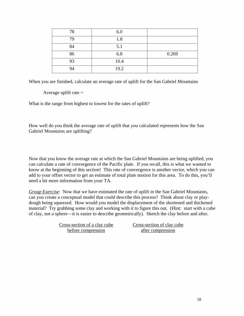
78 6.0 79 1.8 84 5.1 86 6.8 0.269 93 10.4 94 19.2

When you are finished, calculate an average rate of uplift for the San Gabriel Mountains

Average uplift rate = What is the range from highest to lowest for the rates of uplift? How well do you think the average rate of uplift that you calculated represents how the San Gabriel Mountains are uplifting? Now that you know the average rate at which the San Gabriel Mountains are being uplifted, you can calculate a rate of convergence of the Pacific plate. If you recall, this is what we wanted to know at the beginning of this section! This rate of convergence is another vector, which you can add to your offset vector to get an estimate of total plate motion for this area. To do this, you’ll need a bit more information from your TA. Group Exercise: Now that we have estimated the rate of uplift in the San Gabriel Mountains, can you create a conceptual model that could describe this process? Think about clay or play-dough being squeezed. How would you model the displacement of the shortened and thickened material? Try grabbing some clay and working with it to figure this out. (Hint: start with a cube of clay, not a sphere—it is easier to describe geometrically). Sketch the clay before and after.

Cross-section of a clay cube before compression

Cross-section of clay cube after compression

58

Now that you have modeled compression and noted that the clay has thickened upward (uplifted), can you think of a way of relating what you have observed to a mathematical equation using the changing width and height of squares? If you found this a bit challenging, to relate uplift to shortening mathematically, that’s okay. We’ll show you how scientists have created a simple geometrical model to try to relate convergence (the process that results in compression) to uplift. TA Presentation/Discussion: Your TA will walk you through this calculation of convergence using the presentation slides (copied below). Basically, to calculate how much the ground has been “shortened” by convergence, we need to know two more things: 1) the width of the rock that has been uplifted (displaced upward) and 2) the depth to the base of the uplifted rock “blocks” in this area. We’ll explain that point in a moment but first let’s measure the width of the mountains in three places so that an average width can be calculated.

Width of the mountains southeast of their widest = ________ km Width of the mountains at their widest point = ________ km Width of the mountains northwest of the widest = ________ km Average width of mountains = km = ______ _ mm (1 km = 1,000,000 mm) Average uplift rate = _________ mm/yr (calculated on the previous page)

59

As the crust undergoes compression, blocks of rock are wedged upward along faults. We need to know the depth to the zone where the rock’s properties are not such that it will move upward as a block. For this region, we will assume that below approximately 1 km, the rocks no longer behave as coherent blocks like the model above suggests. (Remember to convert km to mm, 1 km = 1000 m = 1,000,000 mm). Finally, you can calculate a convergence rate using the two equations in the diagram above!

(Convergence rate) * (depth of block) = (width of mountains) * (uplift rate)

Convergence rate = ____ _____mm/yr

Orientation of convergence ______________(trend of a line perpendicular to fault)

60

Now you can add the rate of convergence vector to the measured offset vector that you plotted on your graph paper previously. To add this vector to the offset vector, place the tail of the convergence vector on the arrow of the measured offset vector. If you are at all confused, please see the diagram that reviews adding vectors on the following page.

When you have finished adding the vectors, what is the orientation and magnitude of your total plate motion vector? Compare your vector with that of another person’s. Write down the orientation and magnitude of their vector below. How different are they? Do you think that theirs is any less valid than yours? Why or why not?

61

Part VI: Comparing Datasets Group Exercise: Now that you have finally arrived at a total plate motion vector, how does it compare to the Nuvel-1a vector? With you group, discuss how you might explain any differences in 1) vector magnitude and 2) vector orientation. What does this tell you about your model for how the plate boundary behaves? Class Discussion: Where is the missing motion? Part VII: Parting Thoughts Thought Exercise: Which tasks in lab allowed you to come up with answers different from your neighbors? How do human choices impact “objective” results? What opportunities were there for human error in this lab? How variable do you think human error can be? (If two people make the same kind of error, will they have the same amount of error?)

62

When something’s true value is unknown, how would you determine which value is closest to the true value when several people got different answers? How accurately can humans create models that accurately represent how the real world works? Based on your work today, how certain do you think geologists are about how the San Andreas Fault behaves? TA Presentation: As you have witnessed during this exercise, doing science does not always result in neat, clean, tidy answers. In fact, for those of us who pursue a career in science, it is usually this way. Our results are only as good as our ability to gather data precisely and accurately, to make reasonably fitting assumptions, to refine models as new data becomes available and to keep an open mind to new ways and means for learning about the natural world. Science is not as objective as it seems. As we have seen in this exercise, there are many subjective choices and assumptions. How well we do science depends on how honestly we recognize the subjectivity of what we do and how earnestly we strive toward that objective ideal. At the end of the day, we must always remember that objectivity is an ideal for which we strive but we also are human. By the way: Suppose your roommate asked you if California is going to fall into the sea during an earthquake. What would you tell him or her?

63

Plot of Nuvel-1a Plate Motion Vector and Offset and Convergence Vectors Scale: 1” = 10 mm or 1 square = 1 mm

North

64

References Cited (to view the figures and data sources used in these labs see the following references): Computer Animation of the N.E. Pacific and W. North America Plate History, 38 Ma to Present. http://transfer.lsit.ucsb.edu/geol/projects/emvc/cgi-bin/dc/list.cgi?list (8 April, 2004) Aerial photo of San Andreas at Wallace Creek Collier, M., 1999, A Land in Motion, Los Angeles, CA, University of California Press, 118 p. Tectonic map of North America Collier, M., 1999, A Land in Motion, Los Angeles, CA, University of California Press, 118 p. Topographic map of Wallace Creek http://www.scec.org/wallacecreek/exercises/fig1.gif (April 12, 2004) or Sieh, K. E., and Wallace, R. E., 1987, The San Andreas fault at Wallace Creek, San Luis Obispo

County, California: Geological Society of America Centennial Field Guide--Cordilleran Section, p. 233-238.

Evolution of Wallace Creek sketches http://www.scec.org/wallacecreek/paper/ (April8, 2004) or Sieh, K.E., and Jahns, R.H., 1984, Holcene activity of the San Andreas Fault at Wallace Creek,

California: Geological Society of America Bulletin, v. 95, p. 883-896. Geologic Map of Wallace Creek http://www.scec.org/wallacecreek/exercises/fig2.gif (April8, 2004) or Sieh, K.E., and Jahns, R.H., 1984, Holcene activity of the San Andreas Fault at Wallace Creek,

California: Geological Society of America Bulletin, v. 95, p. 883-896. He data and Sampling Sites Spotila, J., House, M., Blythe, A., Niemi, N., & Bank, G., 2002, Controls on the erosion and

geomorphic evolution of the San Bernardino and San Gabriel mountains, southern California. Geological Society of America Special Paper, vol. 365, p. 205-230.

65

Appendix E: Model-driven lab exercise Lab 10: Applying Geologic Methods to Real Issues In the last lab, we looked at the basic structural relationships between rock units. We learned to recognize them as recorded in cross sectional and map views. Today, we will be investigating how these structures can be used to investigate plate motion at plate boundaries. Specifically, we will be using motion along the San Andreas Fault zone to determine the rate at which the Pacific plate is moving in reference to a fixed North American plate. We will begin by exploring the nature of transform plate boundaries and the San Andreas Fault zone. Part l: Transform Plate Boundaries Group Exercise: Let’s start with thinking about the three general types of plate boundaries: convergent, divergent, and transform. You’ve briefly learned about them previously in lab. In the space below, sketch a map view (bird’s eye view from above) of a transform plate boundary. Label the following: Plate A, Plate B, transform fault, and plate motion (draw arrows on the fault that show the relative motion between the plates). What type of motion occurs on the fault (reverse, normal, and/or strike-slip)? ________________ The San Andreas fault zone in southern California is a real life example of this type of plate boundary. It is the boundary between the Pacific and North American plates. Given that the tectonic environment of a transform fault, such as the San Andreas, is largely a shear environment with two plates sliding past each other, would you expect the topography next to the fault to: a) be mountainous,

b) contain valleys or c) be fairly flat and planar?

66

Why? Part ll: The San Andreas Fault: A Big Rip in our Continent Most likely, you are aware of the hazardous nature of the San Andreas Fault zone, but are you aware that many of the devastating earthquakes that occur in California are not on the San Andreas Fault? Why might this be? How are the stresses of plate motion actually distributed across the region beyond the actual San Andreas transform boundary? Are there other faults that Californians should be concerned about? These are the questions that geologists struggle with and seek to answer in many ways. One such investigation is the focus of your lab today. TA Demo/Mini Lecture: Evolution of the San Andreas Fault zone. Your TA will show a computer animation and a map of the San Andreas [see reference list at end of lab assignment]. Group Exercise: Let’s start with the San Andreas Fault. In the space below, sketch at map view (bird’s eye view from above) of the San Andreas transform boundary and the North American and Pacific Plates. Place arrows on the fault that show the relative motion between the two plates (Hint: Los Angeles in becoming a suburb of San Francisco in a few million years).

North In Part I, you discussed what you thought the topography next to a transform fault would look like. Take a look at the aerial photo of the San Andreas Fault in the plastic photo sleeve on your table [see reference list at end of lab assignment]. Is this the topography that you expected to see? Describe what you see and what you expected the topography around the fault to look like.

What I thought the topography around the San Andreas would look like: What the topography around the San Andreas actually looks like:

67

Is there a discrepancy here? If yes, what does this suggest about the nature of the Pacific-North American plate boundary? If you feel there is a disconnect between the model you have learned that describes how transform faults look and work and what you actually see in the photo, you’ve observed what many skeptical geoscientists have observed. The fault just isn’t behaving properly in this area! Turn over your photo sleeve to look at the tectonic map of North America. This photo was taken along the San Andreas Fault to the southwest of the “R” in “SAN ANDREAS FAULT” on the map [see reference list at end of lab assignment]. Describe what is happening to the orientation of the fault in this area. What is the relationship between the orientation of the fault, the orientation of plate motion, and the occurrence of uplift? Group Exercise: Can you imagine how the crust and surface rocks near a bend in a transform fault accommodate strike-slip plate motion? How might movement along the fault affect topography near the bend? To get an idea, use the pieces of cut felt on your table to model movement on the fault. Orient the felt such that the fault is trending northwest. Slowly and very slightly drag the left-hand piece of felt toward the northwest. (This motion replicates the right-lateral motion on the San Andreas Fault.) How does the topography change near the bend in the fault? As you play with the felt, there will probably be several possible geometries of folds and uplifts that develop. Sketch a few of the results showing how the felt accommodates his motion below.

68

Which of the three types of plate boundaries would you expect to observe this kind of topography? Group/Class Exercise: Your observations of how the crust behaves combined with your interpretation of these observations form a descriptive model (a hypothesis) of how the surface and shallow crust might accommodate motion along the San Andreas at the bend. Think this through and describe this model carefully because this is what you will test in the remainder of this exercise. Describe how the upper crust might be accommodating plate motion near the bend in the San Andreas Fault based on your block model above. Use the following terms in your description: strike slip motion, convergence, orientation of the plate boundary, and orientation of the plate motion. The descriptive model (an idea) that you have just formulated should explain why the San Andreas Fault zone is mountainous along the bend in the fault just north of Los Angeles. As you have discovered through this simple exercise, it is the bend that results in a component of convergence. This compressive stress from convergence has lifted the rocks up forming mountains (the San Gabriel and San Bernardino Mountains rise to 10,000 feet above the Los Angeles basin showing that this is indeed a significant process). The term that geoscientists apply to the stress that compresses rocks across a bend in a transform fault is called transpression. Thought Question: If instead of deviating to the west, the bend had deviated to the east instead. To model this with your felt, turn it over such that the felt is oriented to the northeast and move the felt right-laterally. Can you describe or sketch the kind of structure that would form?

69

Interestingly, there is a structure like this to the southeast of the San Andreas bend that we have been studying. Death Valley is the lowest point in North America and it is, in part, a “pull-apart” basin. Death Valley has formed along another right-lateral strike-slip fault zone, the Eastern California Shear Zone that bends easterly. Movement along the bend in this transform-type shear zone has resulted in tensional (pull-apart) instead of compressional stresses. Geoscientists refer to this stress environment as transtensional. Part III: Calculating Plate Motion If you could know any one thing about the San Andreas Fault, I’ll bet you would want to know when and where the next “big one” would occur. So would most geoscientists and probably most of the population of California! While we can’t “know” when this will happen, we can estimate the likelihood of a large quake occurring based on the amount of strain being stored in the rocks adjacent to the fault and our model for how that strain will be released. This stored potential energy can be estimated in part by studying the rate of motion of the two plates that rub shoulders along this transform boundary—the Pacific Plate and the North American Plate. When you think about it this way, calculating these rates and directions of motion becomes far more than an exercise in curiosity—it becomes a necessity for helping us understand how much strain a fault can store before it lets go causing a potentially devastating earthquake. How do scientists calculate plate motions? What models do geologists use to calculate plate motions? If you think about this problem for long, you begin to realize that all plates are moving at different rates and in different directions. Nowhere are they “fixed” relative to a global frame of reference such as the axis of rotation of the globe. The best we can do is to measure relative plate motion between plates and their spreading centers. By determining this relative motion, we can determine rates of slip along other plate boundaries such as along the San Andreas Fault. TA Presentation and Discussion: As you may recall from lecture, the Earth's magnetic field periodically reverses polarity. Such episodes occur relatively rapidly over perhaps a few hundred to a thousand years. As magma erupts from the mid-ocean spreading centers, it cools quickly to form basaltic oceanic crust. Magnetic materials within the cooling lava align with the earth’s magnetic field and become “frozen” in that orientation. When the poles reverse, rocks that cool after the reversal become magnetized in the opposite orientation. This process has produced magnetic “stripes” in the ocean floor. The boundary that separates rocks magnetized in one orientation from those of another is essentially a line in time that can be dated. Using radioactive decay methods, the age of rocks at these boundaries can be determined. If the distance from the spreading center to the reversal also is measured, a spreading rate for the plate relative to the ridge crest can be calculated. If you look closely at a topographic map of the oceanic ridge crest, you’ll notice that there are many transform faults. These faults develop because the ridge crest adds new rocks to the plates at different rates (think of two conveyor belts next to each other moving in the same direction at different speeds—the transform faults would be the boundary separating them.) If you think

70

about the direction of movement of these “conveyor belt” plates, it must be the same as the orientation of the transforms. Using this type of information, the direction and rate of growth for both the North American Plate relative of the Mid-Atlantic Ridge and the Pacific Plate relative to the East Pacific Rise can be estimated. If the rates and directions of motion of these two plates are added together, the result is the rate and direction of motion along the San Andreas Fault. One of the mathematical models that geoscientists have refined and currently use to calculate plate motion from ridge data for all plates all over the world is called the Nuvel-1a plate motion model. According to this model, for the past 0.78 million years, the Pacific Plate has been moving northwest relative to the North American at a rate of 51.1 +/- 2.5 mm/yr and along a trend of N54.0• W +/- 2.7•

direction. But does this rate and direction equate to what is really happening along the San Andreas? Geoscientists tend to be a skeptical bunch because what they see on the ground isn’t necessarily what they predict from their models. In other words, the Earth hasn’t read their book of models so doesn’t always know how to behave! It behaves in a way that we are still trying to understand! Thought Exercise: We need to know how fast and in what direction plates move away from a mid-ocean ridge. What data would you need in order to calculate the rate of movement and the relative motion of the two plates that are being formed along a mid-ocean ridge? Group Exercise: Based on what you know about how transform plate boundaries behave and how plate motion is calculated from mid-ocean ridges, outline how you would calculate plate motion using only information gathered at a transform plate boundary (in this case, at the San Andreas fault zone). Part IV: Determining Rates of Slip along the San Andreas Fault Now that we have an idea (a descriptive model or hypothesis) about how the crust behaves near the bend in the San Andreas, we can test our hypothesis by examining the offset rates in the vicinity of the bend to see whether these rates “add up” to equal the movement along the San Andreas Fault determined by the Nuvel-1a model. Let’s begin by measuring offset rates along the San Andreas.

71

Group/Class Exercise: How might you determine the rate of slip along a transform fault such as the San Andreas? Think of at least two types of information that you would need to know and the kinds of features that might provide it.

Information needed: Features that might provide this information:

If you said you needed to find features that have been offset by the fault that also can be reliably dated, you’re on the right track. Features such as rocks, stream drainages, even mineral deposits are offset along the length of the San Andreas. The trick is getting an age on that feature that reliably indicates when it was last connected across the fault. So, if you know how long ago the feature was last connected across the fault and then if you measure the distance that now separates it, you can estimate an average rate of slip along the fault in that location. So let’s try estimating the rate at which the Pacific plate is moving northwest relative to the North American plate along a portion of the San Andreas in the Carrizo Plain area just north of the bend. We’ll look at the Wallace Creek drainage (see the topographic map of Wallace Creek in the photo sleeve on your table) [see reference list at end of lab assignment]. Notice that Wallace Creek drains across the San Andreas Fault from northeast to southwest. Its downstream portion has been offset periodically by the fault. During the late 1970’s, a graduate student studied these offset stream channels by trenching them and dating the layers of sediment using radiocarbon methods. Results from his research were published thereafter (Sieh and Jahns, 1984). Group Exercise: Based on the evolution of Wallace Creek sketches [see reference list at end of lab assignment], how long ago was the downstream drainage in the lower left hand side of the topographic map aligned with the upstream and active portion of Wallace Creek? years ago. How long ago was the downstream drainage nearer the center of map aligned with the active portion of Wallace Creek? years ago Now that we have the ages of the stream channels, the next step in determining the average rate of slip per year, is to measure the stream offset distances. The amount of offset of the stream channel corresponds with the movement along the fault. Look at the cartoon map of Wallace Creek on the following page. It has been created using modified and simplified data (the scale and orientation have been modified) from the study mentioned above to more clearly illustrate how vectors are used to calculate plate motion. Using the cartoon map on the following page for scale and a ruler, measure the displacement of both the older (Channel B) and younger (Channel A) stream gravels. Convert this distance from feet to millimeters (1”=2.54 cm).

72

Offset distance of older channel (B): _________ft = _________ mm Offset distance of younger channel (A): _________ft = _________ mm Now, use the offset distance and age information to determine the rate of strike-slip motion on the San Andreas Fault. Rates of motion are given in millimeters/year.

Calculate rate of slip for the older channel:

Calculate rate of slip for the younger channel: Are these two rates the same, similar or quite different? . What does this tell you about the rate of slip over time?

Calculate the average slip rate for the two channels and use this value for plotting.

73

Your final step is to use your protractor/ruler to measure the orientation of the San Andreas Fault. Notice that the north arrow on your maps is not pointing to the top of the page.

Orientation of the fault: [**USE N65W**] Now you can combine the rate of slip and direction of slip into a line (a vector) on your graph paper. Notice the scale is given for you (1”+10mm/yr) and North is at the top of the page. This line is a vector because it combines direction and rate information. As you plot this vector, make sure that:

4) the arrow points to the northwest because that is the trend of the Pacific Plate relative to the North American Plate

5) the “tail” of this vector is positioned somewhere in the lower right hand corner 6) the vector is labeled. Label this vector as the “measured offset vector”.

Now we need to calculate the convergence across the San Andreas fault. Part V: Determining Rates of Convergence across the San Andreas Fault Remember the uplift and folding that we predicted near the bend in the San Andreas from the felt exercise? Geoscientists have studied structures in the hills and mountains adjacent to the bend in the San Andreas Fault and have found that they are made up of folds, reverse faults and even wedges and blocks of rocks that are being squeezed upward. Our model assumes that this evidence of compression is caused by the bend in the fault. In this exercise, we’re going to estimate uplift rates adjacent to the fault in the San Gabriel Mountains. Then we’ll convert these uplift rates to a vector representing a rate of convergence and then add that vector to the offset vector we just plotted to see whether the data “adds up” to equal the Nuvel-1a model vector. Group Discussion: Can you think of any ways in which a geologist might measure uplift rates? What information do you need to be able to calculate an uplift rate?

74

TA Presentation and Discussion: Measuring rates of uplift using 4He ages. After your TA has completed his/her presentation, write a general equation to calculate uplift rate below and then test your comprehension by answering the following questions.

10) What happens to the temperature of a rock as it is lifted up from depth toward Earth’s surface?

a. Stays the same b. Increases c. Decreases

11) As a result of this temperature change, what happens to the rate of vibration of atoms that make up the apatite mineral?

a. Stays the same b. Increases c. Decreases

12) Where do the 4He atoms in the apatite come from? a. Radioactive decay of uranium b. Radioactive decay of calcium c. Radioactive decay of phosphorus

13) Why is apatite used for 4He dating? a. Apatite is used because it contains small amounts of uranium b. Apatite is used because it is very rare c. Apatite is used because it is present in bones that are caught up in the fault

14) At what temperature do 4He atoms get “trapped” in an apatite mineral? a. Below 200°C b. Below 70°C c. Below 70°F

15) If the temperature of rocks just below Earth’s surface is 10°C and the geothermal gradient is 30°C/km, how deep is the 4He atom “trapping” temperature?

a. Approximately 1 km below the surface b. Approximately 2 km below the surface c. Approximately 3 km below the surface

16) If an apatite grain in a rock at the Earth’s surface has a 4He age of 10 million years in an area where the geothermal gradient has been measured at 30°C/km (and rocks just below the surface are 10°C), what is its uplift rate?

a. It has been uplifted at a rate of 0.5 mm/yr b. It has been uplifted at a rate of 0.2 mm/yr c. It has been uplifted at a rate of 0.1 mm/yr

17) Scientists calculate that the Himalayas are lifting up at a rate of approximately 10 mm/yr (this is considered fast). How does the uplift rate from question 7 compare to this one?

a. About the same b. Half as fast c. An order of magnitude slower d. Almost two orders of magnitude slower

18) What assumptions did you make in order to do this calculation? Circle all that apply.

75

a. Uplift is and has been occurring at a constant rate over the time frame of 4He ages.

b. A temperature of 10°C reasonably approximates the temperature of rocks just below Earth’s surface for this area.

c. The geothermal gradient increases uniformly to the depth of the trapping temperature and has been constant over the time frame of the 4He ages.

d. The helium atoms are trapped at exactly the trapping temperature. Above that temperature, they all leak out, below that temperature, they are all trapped.

e. The way in which 4He atoms were counted in order to estimate an age is reasonably accurate and precise.

If you circled every point in number 9, you’re right and you were right to be skeptical too! So are most geoscientists. That is why many lines of reasoning and research are brought to bear on an issue as challenging and complex as understanding the tectonics of the San Andreas System. But let’s continue with our study and calculate uplift rates for rocks near the bend in the San Andreas. In the 1990s, several researchers measured 4He ages in apatite grains in rocks collected from the San Gabriel Mountains northwest of the bend in the San Andreas Fault. The location of these sites by sample number and the references to the scientists who did the work are shown on the photo in the sleeve labeled “Sampling Sites from the San Gabriel Mountains” [see reference list at end of lab assignment]. To focus our efforts on understanding how to use uplift data to calculate plate motion, you will be using contrived data based loosely on their experimentally determined 4He ages listed in the table below to calculate uplift rates as you did in problem 7 above. This tweaked data can be found in the table below. Assume a geothermal gradient of 30°C and surface temperature of 15°C. Notice that the surface temperature is different than in the examples on the previous page. Please show your work for the first one, sample #44; then repeat the process to fill in the table.

Rate of Uplift = Depth to the 70°C geotherm/age

Sample Number 4He Age (millions of yrs) Rate of Uplift (mm/yr)

40 12.8 44 3.2 47 10.6 56 4.6 57 12.4

76

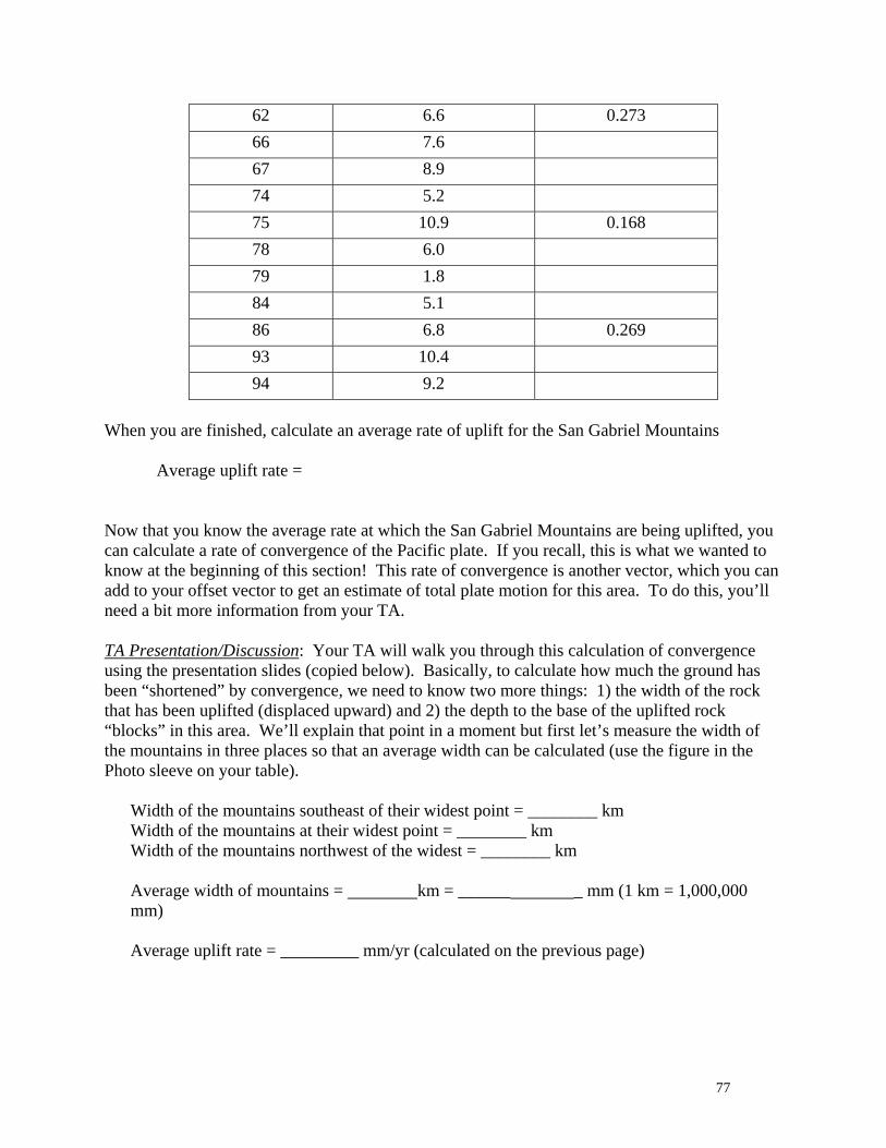
62 6.6 0.273 66 7.6 67 8.9 74 5.2 75 10.9 0.168 78 6.0 79 1.8 84 5.1 86 6.8 0.269 93 10.4 94 9.2

When you are finished, calculate an average rate of uplift for the San Gabriel Mountains

Average uplift rate = Now that you know the average rate at which the San Gabriel Mountains are being uplifted, you can calculate a rate of convergence of the Pacific plate. If you recall, this is what we wanted to know at the beginning of this section! This rate of convergence is another vector, which you can add to your offset vector to get an estimate of total plate motion for this area. To do this, you’ll need a bit more information from your TA. TA Presentation/Discussion: Your TA will walk you through this calculation of convergence using the presentation slides (copied below). Basically, to calculate how much the ground has been “shortened” by convergence, we need to know two more things: 1) the width of the rock that has been uplifted (displaced upward) and 2) the depth to the base of the uplifted rock “blocks” in this area. We’ll explain that point in a moment but first let’s measure the width of the mountains in three places so that an average width can be calculated (use the figure in the Photo sleeve on your table).

Width of the mountains southeast of their widest point = ________ km Width of the mountains at their widest point = ________ km Width of the mountains northwest of the widest = ________ km Average width of mountains = km = ______ _ mm (1 km = 1,000,000 mm) Average uplift rate = _________ mm/yr (calculated on the previous page)

77

As the crust undergoes compression, blocks of rock are wedged upward along faults. We need to know the depth to the zone where the rock’s properties are not such that it will move upward as a block. For this region, we will assume that below approximately 1 km, the rocks no longer behave as coherent blocks like the model above suggests. (Remember to convert km to mm, 1 km = 1000 m = 1,000,000 mm). Finally, you can calculate a convergence rate using the two equations in the diagram above!

(Convergence rate) * (depth of block) = (width of mountains) * (uplift rate)

Convergence rate = ____ _____mm/yr

78

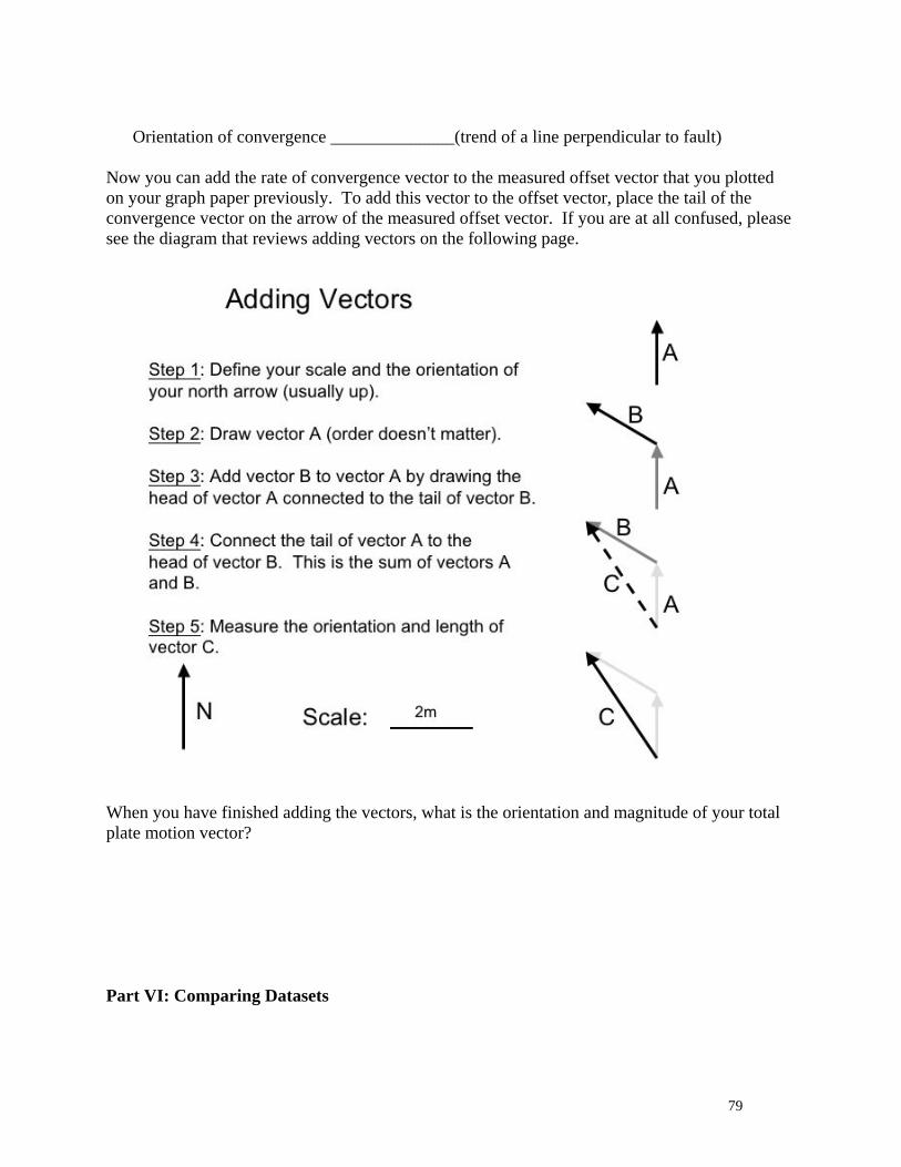
Orientation of convergence ______________(trend of a line perpendicular to fault)

Now you can add the rate of convergence vector to the measured offset vector that you plotted on your graph paper previously. To add this vector to the offset vector, place the tail of the convergence vector on the arrow of the measured offset vector. If you are at all confused, please see the diagram that reviews adding vectors on the following page.

When you have finished adding the vectors, what is the orientation and magnitude of your total plate motion vector? Part VI: Comparing Datasets

79

Group Exercise: Recall the Nuvel-1A model data described at the end of Part III? Now let’s plot the trend and rate of movement of the San Andreas as accurately as possible by plotting that information on the graph paper handed out with this exercise. All you need to do is draw a line on the paper that is oriented with respect to the fault’s trend and is exactly as long as the annual plate motion. Notice that a scale is given for you (1” = 10 mm/year) and north is at the top of the page. Make sure that you start your vector at the same point you started your first vector. According to this model, for the past 0.78 million years, the Pacific Plate has been moving northwest relative to the North American at a rate of 51.1 +/- 2.5 mm/yr and along a trend of N54.0• W +/- 2.7• direction. Group Exercise: How does the total plate motion vector you calculated using transform plate boundary data compare to the NUVEL-1A plate motion vector that was calculated using divergent mid-ocean ridge data? With you group, discuss how you might explain any differences in 1) vector magnitude and 2) vector orientation. Thought Question: If you calculated a slip vector that equaled the NUVEL-1A vector in both magnitude and orientation, what would that tell you about the transform boundary? (Hint: What does it indicate isn’t happening?) Class Discussion: Where is the missing motion?

80

Part VII: Parting Thoughts Thought Exercise: As you may or may not have noticed during this exercise, much of the data you used had been modified to better illustrate how a geometric model to accommodate transpression can be used to calculate plate motion. Doing science does not always result in neat, clean, tidy answers such as those that you have calculated in this exercise. In fact, for those of us who pursue a career in science, it usually never does. If the data that you used had not been modified and didn’t work out as “perfectly” (e.g., plate motion could not be explained using a simple combination of uplift and offset data), would you be more likely to question the plate tectonic models that we use to understand plate motion? By the way: Suppose your roommate asked you if California is going to fall into the sea during an earthquake. What would you tell him or her?

81

Plot of Nuvel-1a Plate Motion Vector and Offset and Convergence Vectors Scale: 1” = 10 mm or 1 square = 1 mm

North

82

References Cited (to view the figures and data sources used in these labs see the following references): Computer Animation of the N.E. Pacific and W. North America Plate History, 38 Ma to Present. http://transfer.lsit.ucsb.edu/geol/projects/emvc/cgi-bin/dc/list.cgi?list (April8, 2004) Aerial photo of San Andreas at Wallace Creek Collier, M., 1999, A Land in Motion, Los Angeles, CA, University of California Press, 118 p. Tectonic map of North America Collier, M., 1999, A Land in Motion, Los Angeles, CA, University of California Press, 118 p. Topographic map of Wallace Creek http://www.scec.org/wallacecreek/exercises/fig1.gif (April 12, 2004) or Sieh, K. E., and Wallace, R. E., 1987, The San Andreas fault at Wallace Creek, San Luis Obispo County, California: Geological Society of America Centennial Field Guide--Cordilleran Section, p. 233-238. Evolution of Wallace Creek sketches http://www.scec.org/wallacecreek/paper/ (April8, 2004) or Sieh, K.E., and Jahns, R.H., 1984, Holcene activity of the San Andreas Fault at Wallace Creek, California: Geological Society of America Bulletin, v. 95, p. 883-896. He data and Sampling Sites Spotila, J., House, M., Blythe, A., Niemi, N., & Bank, G., 2002, Controls on the erosion and

geomorphic evolution of the San Bernardino and San Gabriel mountains, southern California. Geological Society of America Special Paper, vol. 365, p. 205-230.

83

Appendix F: Summary of student questionnaire responses (Session II) Letter - # - Approach = TA - section - approach

A-1-data Data real? (Yes-No) 12-2 86% Science: (~8 made comments) subjective, error, scientists will come up with different results "scientists can try to predict plate motion, but there are always other factors that they do not include" "data isn't always accurate" "research is subjective, depends on the researcher" E-1-data Data real? (Yes-No) 14-7 67% Science: (majority~12 made comments) subjective, error, scientists will argue/discuss different results and come up with the one that works the best "scientists probably argue over measurements" "results are only as accurate as the measurements" "scientific research is prone to error" "it isn't exact" Other: Lab hard, calculations hard D-1-data Data real? (Yes-No) 16-5 76% Science: (16 made comments) Subjective, error, different, but valid results "not everything can be 100% proven" "it is difficult to get an exact, guaranteed answer." "scientific research can sometimes be subjective to the researcher." "very subjective, but can still be accurate" Other: "I don't think the lab gave us much of a flavor of what it is to be a geologist making these measurements in the field, though I know that is difficult to do in a classroom." Calculations and plotting difficult, different teaching style refreshing "it was harder, but i learned more." Liked teacher-student interactions "required deeper understanding in order to keep up. If you didn't understand, it was hard to get anything done."

84

"learned to think more about what we did" "I liked it better because it was much more realistic." "had more of a geology feel than simply classifying rocks" A-2-data Data Real? (Yes-No) 17-4 81% Science: (18 made comments) Error, need for many data points, accuracy, revisions "how to find error and improve methods" "there are tons of variables and its hard to be accurate" "that it is hard to get accurate and exactly the same results as others" "models vary, answers vary, science is an uncertainty" Other: Frustrated with not knowing exactly where to measure (having to decide themselves) Repetitive 1 or 2 thought the math/vectors was difficult "a refreshment on the scientific method" D-2-data Data real? (Yes-No) 15-6 71% Science: Human error, debate/differing opinion, uncertain, flexible "science is usually a best guess with the best resources available" "is founded on the debate of research" "nothing is certain, everything can be revised and changed" "it should never be considered 100% correct" B-1-modelData real? (Yes-No) 12-9 57% Science: (~5 made comments) subjective, error/inaccurate "there is more than one right answer to a problem" Other: calculations hard, confusing/not explained well "did not [learn much about science and scientific research] because we didn't use natural data" required a lot more TA assistance than other labs didn't understand the overall purpose too complex, resulting in understanding little to nothing lab wording confusing C-1-model

85

Data real? (Yes-No) 17-7 71% Science: ( 8 made comments) Not accurate/error, scientists make assumptions "It involves a lot of guessing and estimating" "not all data is accurate" "that is always rests on certain assumptions' Other: Vectors/calculations hard B-2-model Data real? (Yes-No) 11-8 61% Science: (only 3 made comments) Error "it can be not perfect even with advanced tools" Other: Lab hard, calculations hard, confusing because TA didn't explain things clearly B-3-model Data real? (Yes-No) 11-5 69% Science: (only 5 made comments) "it is not always accurate and precise" "science is not perfect" "mistakes can be made and many tests need to be done" "there are many uncertainties" Other: "it was more work with more calculations, but gave a more realistic approach" "it was more difficult to understand, but when you get it, it is very easy to apply to other geologic areas" "a bunch of guess work versus facts (previous labs)" vectors hard, 2 comments about TA clarification

86

Appendix G: Summary of statistical results (Sessions I & II) Existing Lab pre/posttest mean comparison (Session I) Time 0 = pretest Time 1 = posttest NOS# refers to nature of science question from survey Content = total content score (out of 9)

Report

3.12 4.02 3.47 3.71 4.25 4.17 3.97 3.34 3.05 4.13 3.47 3.84161 161 161 161 161 161 161 161 160 161 161 160

1.23 .86 1.13 1.15 1.03 1.05 1.01 1.10 1.21 .92 1.25 1.74.211 -1.068 -.615 -.610 -1.548 -1.449 -1.010 -.237 -.249 -1.349 -.203 -.066

-1.215 1.486 -.300 -.682 2.053 1.658 .762 -.890 -.945 2.184 -1.153 .0091.509 .737 1.276 1.330 1.053 1.095 1.018 1.199 1.457 .839 1.563 3.0303.43 4.12 3.61 3.82 4.40 4.11 3.89 3.48 3.39 4.22 3.50 4.02160 161 161 161 161 161 161 160 161 161 161 158

1.15 .92 1.02 1.24 .95 1.08 1.00 1.06 1.16 .93 1.25 1.74-.055 -1.224 -.585 -.848 -1.890 -1.249 -.895 -.204 -.518 -1.789 -.269 .074

-1.287 1.577 -.170 -.365 3.563 .965 .607 -.994 -.503 3.810 -1.126 -.3551.329 .847 1.040 1.536 .903 1.158 .995 1.132 1.352 .862 1.564 3.0123.28 4.07 3.54 3.77 4.33 4.14 3.93 3.41 3.22 4.18 3.48 3.93321 322 322 322 322 322 322 321 321 322 322 318

1.20 .89 1.08 1.20 .99 1.06 1.00 1.08 1.20 .92 1.25 1.74.064 -1.134 -.618 -.728 -1.698 -1.340 -.946 -.225 -.379 -1.558 -.235 .003

-1.269 1.464 -.206 -.532 2.646 1.248 .645 -.925 -.777 2.888 -1.142 -.1711.439 .792 1.159 1.432 .981 1.124 1.005 1.167 1.429 .850 1.559 3.020

MeanNStd. DeviationSkewnessKurtosisVarianceMeanNStd. DeviationSkewnessKurtosisVarianceMeanNStd. DeviationSkewnessKurtosisVariance

TIME0

1

Total

NOS11 NOS12 NOS13 NOS14 NOS15 NOS16 NOS17 NOS18 NOS19 NOS20 NOS21 CONTENT

87

ANOVA Table

7.565 1 7.565 5.330 .022452.759 319 1.419460.324 320

.795 1 .795 1.004 .317253.416 320 .792254.211 321

1.503 1 1.503 1.298 .255370.472 320 1.158371.975 321

.898 1 .898 .626 .429458.634 320 1.433459.531 321

1.643 1 1.643 1.679 .196313.118 320 .978314.761 321

.376 1 .376 .334 .564360.335 320 1.126360.711 321

.447 1 .447 .444 .506322.050 320 1.006322.497 321

1.707 1 1.707 1.464 .227371.832 319 1.166373.539 320

9.348 1 9.348 6.657 .010447.948 319 1.404457.296 320

.699 1 .699 .821 .365272.211 320 .851272.910 321

.112 1 .112 .072 .789500.311 320 1.563500.422 321

2.618 1 2.618 .867 .353954.718 316 3.021957.336 317

(Combined)Between GroupsWithin GroupsTotal

(Combined)Between GroupsWithin GroupsTotal

(Combined)Between GroupsWithin GroupsTotal

(Combined)Between GroupsWithin GroupsTotal

(Combined)Between GroupsWithin GroupsTotal

(Combined)Between GroupsWithin GroupsTotal

(Combined)Between GroupsWithin GroupsTotal

(Combined)Between GroupsWithin GroupsTotal

(Combined)Between GroupsWithin GroupsTotal

(Combined)Between GroupsWithin GroupsTotal

(Combined)Between GroupsWithin GroupsTotal

(Combined)Between GroupsWithin GroupsTotal

NOS11 * TIME

NOS12 * TIME

NOS13 * TIME

NOS14 * TIME

NOS15 * TIME

NOS16 * TIME

NOS17 * TIME

NOS18 * TIME

NOS19 * TIME

NOS20 * TIME

NOS21 * TIME

CONTENT * TIME

Sum ofSquares df Mean Square F Sig.

Data-driven pre/posttest mean comparison (Session I)

88

Time 0 = pretest Time 1 = posttest NOS# refers to nature of science question from survey Content = total content score (out of 9)

Report

2.96 4.04 3.75 3.70 4.30 4.32 4.07 3.26 3.12 4.15 3.60 4.14191 191 191 191 191 191 191 191 191 191 191 191

1.21 .93 .96 1.23 1.01 1.03 .92 1.02 1.15 .80 1.23 1.641.461 .872 .923 1.518 1.013 1.052 .847 1.047 1.328 .645 1.504 2.676

-1.103 .807 -.300 -.244 3.079 3.019 .320 -.932 -.649 1.163 -.899 .054.388 -1.064 -.531 -.870 -1.799 -1.840 -.842 -.217 -.384 -.960 -.429 -.3163.40 4.34 3.92 4.01 4.37 4.11 3.98 3.58 3.43 4.43 3.73 6.14188 188 188 188 188 188 187 188 188 188 188 188

1.19 .92 .97 1.06 1.05 1.01 .95 1.05 1.13 .83 1.23 1.721.419 .855 .940 1.134 1.100 1.020 .908 1.101 1.284 .685 1.504 2.943

-1.428 3.875 1.048 .013 2.835 1.703 .293 -1.023 -.420 4.188 -.924 .411-.039 -1.865 -1.013 -.908 -1.850 -1.361 -.796 -.242 -.551 -1.865 -.541 -.5903.18 4.19 3.84 3.85 4.34 4.22 4.03 3.42 3.27 4.29 3.66 5.13379 379 379 379 379 379 378 379 379 379 379 379

1.22 .94 .97 1.16 1.03 1.02 .94 1.05 1.15 .83 1.23 1.951.486 .883 .936 1.348 1.054 1.045 .877 1.096 1.327 .683 1.504 3.806

-1.329 1.914 .269 -.011 2.880 2.176 .292 -.949 -.566 2.217 -.922 -.226.164 -1.401 -.760 -.922 -1.813 -1.571 -.818 -.210 -.457 -1.348 -.481 -.234

MeanNStd. DeviationVarianceKurtosisSkewnessMeanNStd. DeviationVarianceKurtosisSkewnessMeanNStd. DeviationVarianceKurtosisSkewness

TIME0

1

Total

NOS11 NOS12 NOS13 NOS14 NOS15 NOS16 NOS17 NOS18 NOS19 NOS20 NOS21 CONTENT

89

ANOVA Table

18.858 1 18.858 13.094 .000542.942 377 1.440561.799 378

8.146 1 8.146 9.433 .002325.553 377 .864333.699 378

2.620 1 2.620 2.812 .094351.238 377 .932353.858 378

9.359 1 9.359 7.052 .008500.366 377 1.327509.726 378

.380 1 .380 .360 .549398.063 377 1.056398.443 378

4.295 1 4.295 4.146 .042390.529 377 1.036394.823 378

.754 1 .754 .860 .354329.926 376 .877330.680 377

9.581 1 9.581 8.925 .003404.714 377 1.074414.296 378

9.130 1 9.130 6.991 .009492.331 377 1.306501.462 378

7.376 1 7.376 11.092 .001250.698 377 .665258.074 378

1.519 1 1.519 1.010 .315566.924 377 1.504568.443 378379.800 1 379.800 135.225 .000

1058.865 377 2.8091438.665 378

(Combined)Between GroupsWithin GroupsTotal

(Combined)Between GroupsWithin GroupsTotal

(Combined)Between GroupsWithin GroupsTotal

(Combined)Between GroupsWithin GroupsTotal

(Combined)Between GroupsWithin GroupsTotal

(Combined)Between GroupsWithin GroupsTotal

(Combined)Between GroupsWithin GroupsTotal

(Combined)Between GroupsWithin GroupsTotal

(Combined)Between GroupsWithin GroupsTotal

(Combined)Between GroupsWithin GroupsTotal

(Combined)Between GroupsWithin GroupsTotal

(Combined)Between GroupsWithin GroupsTotal

NOS11 * TIME

NOS12 * TIME

NOS13 * TIME

NOS14 * TIME

NOS15 * TIME

NOS16 * TIME

NOS17 * TIME

NOS18 * TIME

NOS19 * TIME

NOS20 * TIME

NOS21 * TIME

CONTENT * TIME

Sum ofSquares df Mean Square F Sig.

Existing Lab and Data-driven lab pretest mean comparison (Session I)

90

Time 0 = pretest Time 1 = posttest NOS# refers to nature of science question from survey Content = total content score (out of 9)

Report

3.12 4.02 3.47 3.71 4.25 4.17 3.97 3.34 3.05 4.13 3.47 3.84161 161 161 161 161 161 161 161 160 161 161 1601.23 .86 1.13 1.15 1.03 1.05 1.01 1.10 1.21 .92 1.25 1.74

1.509 .737 1.276 1.330 1.053 1.095 1.018 1.199 1.457 .839 1.563 3.030-1.215 1.486 -.300 -.682 2.053 1.658 .762 -.890 -.945 2.184 -1.153 .009

.211 -1.068 -.615 -.610 -1.548 -1.449 -1.010 -.237 -.249 -1.349 -.203 -.0662.96 4.04 3.75 3.70 4.30 4.32 4.07 3.26 3.12 4.15 3.60 4.15191 191 191 191 191 191 191 191 191 191 191 1891.21 .93 .96 1.23 1.01 1.03 .92 1.02 1.15 .80 1.23 1.64

1.461 .872 .923 1.518 1.013 1.052 .847 1.047 1.328 .645 1.504 2.680-1.103 .807 -.300 -.244 3.079 3.019 .320 -.932 -.649 1.163 -.899 .071

.388 -1.064 -.531 -.870 -1.799 -1.840 -.842 -.217 -.384 -.960 -.429 -.3293.03 4.03 3.62 3.70 4.28 4.26 4.03 3.30 3.09 4.14 3.54 4.01352 352 352 352 352 352 352 352 351 352 352 3491.22 .90 1.05 1.20 1.01 1.04 .96 1.06 1.18 .86 1.24 1.69

1.486 .808 1.101 1.428 1.029 1.074 .925 1.115 1.384 .732 1.531 2.856-1.167 1.053 -.136 -.409 2.529 2.255 .608 -.907 -.802 1.820 -1.038 -.010

.305 -1.061 -.631 -.763 -1.673 -1.640 -.940 -.219 -.321 -1.183 -.323 -.210

MeanNStd. DeviationVarianceKurtosisSkewnessMeanNStd. DeviationVarianceKurtosisSkewnessMeanNStd. DeviationVarianceKurtosisSkewness

TRT0

1

Total

NOS11 NOS12 NOS13 NOS14 NOS15 NOS16 NOS17 NOS18 NOS19 NOS20 NOS21 CONTENT

91

ANOVA Table

2.410 1 2.410 1.625 .203519.180 350 1.483521.591 351

.025 1 .025 .031 .860283.566 350 .810283.591 351

6.941 1 6.941 6.401 .012379.559 350 1.084386.500 351

.028 1 .028 .020 .889501.245 350 1.432501.273 351

.210 1 .210 .203 .652360.946 350 1.031361.156 351

1.984 1 1.984 1.852 .174375.005 350 1.071376.989 351

.951 1 .951 1.028 .311323.819 350 .925324.770 351

.474 1 .474 .424 .515390.799 350 1.117391.273 351

.432 1 .432 .311 .577483.830 349 1.386484.262 350

.040 1 .040 .055 .816256.858 350 .734256.898 351

1.622 1 1.622 1.059 .304535.821 350 1.531537.443 351

8.362 1 8.362 2.944 .087985.627 347 2.840993.989 348

(Combined)Between GroupsWithin GroupsTotal

(Combined)Between GroupsWithin GroupsTotal

(Combined)Between GroupsWithin GroupsTotal

(Combined)Between GroupsWithin GroupsTotal

(Combined)Between GroupsWithin GroupsTotal

(Combined)Between GroupsWithin GroupsTotal

(Combined)Between GroupsWithin GroupsTotal

(Combined)Between GroupsWithin GroupsTotal

(Combined)Between GroupsWithin GroupsTotal

(Combined)Between GroupsWithin GroupsTotal

(Combined)Between GroupsWithin GroupsTotal

(Combined)Between GroupsWithin GroupsTotal

NOS11 * TRT

NOS12 * TRT

NOS13 * TRT

NOS14 * TRT

NOS15 * TRT

NOS16 * TRT

NOS17 * TRT

NOS18 * TRT

NOS19 * TRT

NOS20 * TRT

NOS21 * TRT

CONTENT * TRT

Sum ofSquares df Mean Square F Sig.

Model-driven lab pre/posttest mean comparison (Session II)

92

Time 0 = pretest Time 1 = posttest NOS# refers to nature of science question from survey Content = total content score (out of 9)

Report

3.18 4.11 3.90 3.55 4.30 4.05 3.93 3.59 3.03 3.60 4.19 3.671273 73 73 73 73 73 73 73 73 73 73 73

1.31 .94 1.03 1.28 1.01 1.04 1.00 1.22 1.27 .95 .86 1.95121.704 .877 1.060 1.640 1.019 1.080 1.009 1.495 1.610 .909 .740 3.807

-1.339 1.206 1.108 -.961 1.750 1.746 .008 -.836 -1.047 .218 1.852 -.534.084 -1.163 -1.138 -.477 -1.476 -1.409 -.790 -.423 -.136 -.599 -1.192 -.0523.34 4.85 4.52 3.96 4.88 4.86 4.85 3.86 4.62 4.77 4.93 6.1918

73 73 73 73 73 73 73 73 73 73 73 731.31 .46 .73 1.10 .41 .45 .46 1.07 .70 .54 .35 2.0115

1.728 .213 .531 1.207 .165 .203 .213 1.148 .490 .292 .120 4.046-1.234 9.412 -.070 .579 12.247 10.904 9.412 -1.023 .903 4.348 26.723 .019

-.250 -3.167 -1.181 -1.080 -3.504 -3.399 -3.167 -.486 -1.555 -2.294 -5.205 -.8603.26 4.48 4.21 3.75 4.59 4.46 4.39 3.73 3.82 4.18 4.56 4.9315146 146 146 146 146 146 146 146 146 146 146 146

1.31 .82 .94 1.21 .82 .90 .90 1.15 1.30 .97 .75 2.34491.711 .679 .886 1.456 .671 .802 .819 1.331 1.678 .938 .565 5.499

-1.315 3.054 1.582 -.448 5.073 4.245 1.544 -.826 -.522 .565 4.124 -.846-.082 -1.771 -1.294 -.755 -2.236 -2.037 -1.479 -.484 -.801 -1.073 -1.941 -.245

MeanNStd. DeviationVarianceKurtosisSkewnessMeanNStd. DeviationVarianceKurtosisSkewnessMeanNStd. DeviationVarianceKurtosisSkewness

TIME0

1

Total

PROVE UNCERT CREATIVE CHANGE POORLY OLD IMPORT ACCURATE SUBJECT DIFFER ARGUE CONTENT

93

ANOVA Table

.986 1 .986 .575 .450247.123 144 1.716248.110 145

19.973 1 19.973 36.654 .00078.466 144 .54598.438 14513.870 1 13.870 17.436 .000

114.548 144 .795128.418 145

6.164 1 6.164 4.331 .039204.959 144 1.423211.123 145

12.082 1 12.082 20.406 .00085.260 144 .59297.342 14523.842 1 23.842 37.153 .00092.411 144 .642

116.253 14530.747 1 30.747 50.313 .00088.000 144 .611

118.747 1452.740 1 2.740 2.073 .152

190.301 144 1.322193.041 145

92.164 1 92.164 87.772 .000151.205 144 1.050243.370 145

49.486 1 49.486 82.362 .00086.521 144 .601

136.007 14519.973 1 19.973 46.408 .00061.973 144 .43081.945 145

231.890 1 231.890 59.057 .000565.425 144 3.927797.315 145

(Combined)Between GroupsWithin GroupsTotal

(Combined)Between GroupsWithin GroupsTotal

(Combined)Between GroupsWithin GroupsTotal

(Combined)Between GroupsWithin GroupsTotal

(Combined)Between GroupsWithin GroupsTotal

(Combined)Between GroupsWithin GroupsTotal

(Combined)Between GroupsWithin GroupsTotal

(Combined)Between GroupsWithin GroupsTotal

(Combined)Between GroupsWithin GroupsTotal

(Combined)Between GroupsWithin GroupsTotal

(Combined)Between GroupsWithin GroupsTotal

(Combined)Between GroupsWithin GroupsTotal

PROVE * TIME

UNCERT * TIME

CREATIVE * TIME

CHANGE * TIME

POORLY * TIME

OLD * TIME

IMPORT * TIME

ACCURATE * TIME

SUBJECT * TIME

DIFFER * TIME

ARGUE * TIME

CONTENT * TIME

Sum ofSquares df Mean Square F Sig.

Data-driven pre/posttest mean comparison (Session II)

94

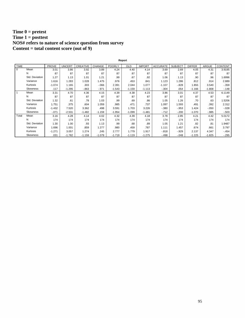
Time 0 = pretest Time 1 = posttest NOS# refers to nature of science question from survey Content = total content score (out of 9)

Report

3.01 3.86 3.92 3.89 4.24 4.40 4.14 3.69 2.69 4.05 4.31 3.919587 87 87 87 87 87 87 87 87 87 87 87

1.27 1.13 1.01 1.21 .99 .67 .92 1.06 1.13 .90 .96 1.69961.616 1.283 1.028 1.475 .976 .453 .841 1.123 1.286 .812 .914 2.889

-1.074 1.165 .303 -.066 2.391 2.044 1.077 -1.107 -.828 1.855 3.540 -.359.117 -1.295 -.863 -.971 -1.543 -1.159 -1.113 -.304 .054 -1.166 -1.808 -.1483.31 4.70 4.36 4.15 4.39 4.38 4.23 3.86 3.01 4.37 4.53 6.1149

87 87 87 87 87 87 87 87 87 87 87 871.32 .61 .78 1.03 .99 .69 .86 1.05 1.26 .70 .63 1.5206

1.751 .375 .604 1.059 .985 .471 .737 1.097 1.593 .491 .392 2.312-1.432 7.520 3.362 .498 3.591 1.703 3.226 -.380 -.953 1.424 -.050 -.028

-.071 -2.531 -1.482 -1.159 -1.954 -1.099 -1.481 -.712 -.200 -1.070 -.985 -.5033.16 4.28 4.14 4.02 4.32 4.39 4.18 3.78 2.85 4.21 4.42 5.0172174 174 174 174 174 174 174 174 174 174 174 174

1.30 1.00 .93 1.13 .99 .68 .89 1.05 1.21 .82 .81 1.94871.696 1.001 .859 1.277 .980 .459 .787 1.111 1.457 .674 .661 3.797

-1.271 3.057 1.274 .245 2.777 1.779 1.917 -.818 -.929 2.137 4.347 -.454.031 -1.782 -1.159 -1.079 -1.719 -1.119 -1.275 -.498 -.048 -1.225 -1.825 -.295

MeanNStd. DeviationVarianceKurtosisSkewnessMeanNStd. DeviationVarianceKurtosisSkewnessMeanNStd. DeviationVarianceKurtosisSkewness

TIME0

1

Total

PROVE UNCERT CREATIVE CHANGE POORLY OLD IMPORT ACCURATE SUBJECT DIFFER ARGUE CONTENT

95

ANOVA Table

3.885 1 3.885 2.307 .131289.609 172 1.684293.494 173

30.626 1 30.626 36.947 .000142.575 172 .829173.201 173

8.299 1 8.299 10.167 .002140.391 172 .816148.690 173

3.040 1 3.040 2.400 .123217.908 172 1.267220.948 173

.971 1 .971 .991 .321168.644 172 .980169.615 173

.023 1 .023 .050 .82479.402 172 .46279.425 173

.368 1 .368 .466 .496135.747 172 .789136.115 173

1.293 1 1.293 1.165 .282190.966 172 1.110192.259 173

4.506 1 4.506 3.130 .079247.609 172 1.440252.115 173

4.506 1 4.506 6.917 .009112.046 172 .651116.552 173

2.075 1 2.075 3.178 .076112.299 172 .653114.374 173209.661 1 209.661 80.623 .000447.287 172 2.601656.948 173

(Combined)Between GroupsWithin GroupsTotal

(Combined)Between GroupsWithin GroupsTotal

(Combined)Between GroupsWithin GroupsTotal

(Combined)Between GroupsWithin GroupsTotal

(Combined)Between GroupsWithin GroupsTotal

(Combined)Between GroupsWithin GroupsTotal

(Combined)Between GroupsWithin GroupsTotal

(Combined)Between GroupsWithin GroupsTotal

(Combined)Between GroupsWithin GroupsTotal

(Combined)Between GroupsWithin GroupsTotal

(Combined)Between GroupsWithin GroupsTotal

(Combined)Between GroupsWithin GroupsTotal

PROVE * TIME

UNCERT * TIME

CREATIVE * TIME

CHANGE * TIME

POORLY * TIME

OLD * TIME

IMPORT * TIME

ACCURATE * TIME

SUBJECT * TIME

DIFFER * TIME

ARGUE * TIME

CONTENT * TIME

Sum ofSquares df Mean Square F Sig.

Model-driven and Data-driven pretest mean comparison (Session II)

96

Time 0 = pretest Time 1 = posttest NOS# refers to nature of science question from survey Content = total content score (out of 9)

Report

3.18 4.11 3.90 3.55 4.30 4.05 3.93 3.59 3.03 3.60 4.19 3.671273 73 73 73 73 73 73 73 73 73 73 73

1.31 .94 1.03 1.28 1.01 1.04 1.00 1.22 1.27 .95 .86 1.95121.704 .877 1.060 1.640 1.019 1.080 1.009 1.495 1.610 .909 .740 3.807

-1.339 1.206 1.108 -.961 1.750 1.746 .008 -.836 -1.047 .218 1.852 -.534.084 -1.163 -1.138 -.477 -1.476 -1.409 -.790 -.423 -.136 -.599 -1.192 -.0523.01 3.86 3.92 3.89 4.24 4.40 4.14 3.69 2.69 4.05 4.31 3.9195

87 87 87 87 87 87 87 87 87 87 87 871.27 1.13 1.01 1.21 .99 .67 .92 1.06 1.13 .90 .96 1.6996

1.616 1.283 1.028 1.475 .976 .453 .841 1.123 1.286 .812 .914 2.889-1.074 1.165 .303 -.066 2.391 2.044 1.077 -1.107 -.828 1.855 3.540 -.359

.117 -1.295 -.863 -.971 -1.543 -1.159 -1.113 -.304 .054 -1.166 -1.808 -.1483.09 3.98 3.91 3.73 4.27 4.24 4.04 3.64 2.84 3.84 4.26 3.8063160 160 160 160 160 160 160 160 160 160 160 1601.29 1.05 1.02 1.25 1.00 .87 .96 1.13 1.21 .95 .91 1.8171

1.653 1.106 1.036 1.569 .990 .764 .923 1.287 1.453 .900 .833 3.302-1.193 1.402 .625 -.615 1.980 3.085 .445 -.883 -.952 .677 2.720 -.441

.105 -1.296 -.982 -.722 -1.493 -1.584 -.951 -.388 .000 -.845 -1.537 -.122

MeanNStd. DeviationVarianceKurtosisSkewnessMeanNStd. DeviationVarianceKurtosisSkewnessMeanNStd. DeviationVarianceKurtosisSkewness

TRT1

2

Total

PROVE UNCERT CREATIVE CHANGE POORLY OLD IMPORT ACCURATE SUBJECT DIFFER ARGUE CONTENT

97

ANOVA Table

1.102 1 1.102 .665 .416261.673 158 1.656262.775 159

2.432 1 2.432 2.215 .139173.468 158 1.098175.900 159

.009 1 .009 .009 .924164.766 158 1.043164.775 159

4.511 1 4.511 2.910 .090244.933 158 1.550249.444 159

.143 1 .143 .143 .705157.301 158 .996157.444 159

4.793 1 4.793 6.490 .012116.700 158 .739121.494 159

1.691 1 1.691 1.843 .177145.002 158 .918146.694 159

.402 1 .402 .311 .578204.292 158 1.293204.694 159

4.528 1 4.528 3.158 .077226.566 158 1.434231.094 159

7.798 1 7.798 9.107 .003135.296 158 .856143.094 159

.558 1 .558 .668 .415131.936 158 .835132.494 159

2.447 1 2.447 .740 .391522.546 158 3.307524.994 159

(Combined)Between GroupsWithin GroupsTotal

(Combined)Between GroupsWithin GroupsTotal

(Combined)Between GroupsWithin GroupsTotal

(Combined)Between GroupsWithin GroupsTotal

(Combined)Between GroupsWithin GroupsTotal

(Combined)Between GroupsWithin GroupsTotal

(Combined)Between GroupsWithin GroupsTotal

(Combined)Between GroupsWithin GroupsTotal

(Combined)Between GroupsWithin GroupsTotal

(Combined)Between GroupsWithin GroupsTotal

(Combined)Between GroupsWithin GroupsTotal

(Combined)Between GroupsWithin GroupsTotal

PROVE * TRT

UNCERT * TRT

CREATIVE * TRT

CHANGE * TRT

POORLY * TRT

OLD * TRT

IMPORT * TRT

ACCURATE * TRT

SUBJECT * TRT

DIFFER * TRT

ARGUE * TRT

CONTENT * TRT

Sum ofSquares df Mean Square F Sig.

98