Analysis of optically thin linesobserved by IRIS

Release 1.0

Vanessa Polito and Paola Testa

Oct 28, 2019

CONTENTS

1 Introduction 1

2 Formation of optically thin lines 32.1 Excitation and de-excitation of atomic levels . . . . . . . . . . . . . . . . . . . . . . . . . . . . . . 32.2 Ionization/Recombination . . . . . . . . . . . . . . . . . . . . . . . . . . . . . . . . . . . . . . . . 42.3 Line intensity and contribution function . . . . . . . . . . . . . . . . . . . . . . . . . . . . . . . . . 62.4 Non-equilibrium effects . . . . . . . . . . . . . . . . . . . . . . . . . . . . . . . . . . . . . . . . . 7

3 Optically-thin lines observed by IRIS 113.1 O I . . . . . . . . . . . . . . . . . . . . . . . . . . . . . . . . . . . . . . . . . . . . . . . . . . . . 113.2 Cl I . . . . . . . . . . . . . . . . . . . . . . . . . . . . . . . . . . . . . . . . . . . . . . . . . . . . 123.3 Si IV . . . . . . . . . . . . . . . . . . . . . . . . . . . . . . . . . . . . . . . . . . . . . . . . . . . 123.4 O IV, S IV . . . . . . . . . . . . . . . . . . . . . . . . . . . . . . . . . . . . . . . . . . . . . . . . 123.5 Fe XII . . . . . . . . . . . . . . . . . . . . . . . . . . . . . . . . . . . . . . . . . . . . . . . . . . . 143.6 Fe XXI . . . . . . . . . . . . . . . . . . . . . . . . . . . . . . . . . . . . . . . . . . . . . . . . . . 14

4 Analysis of IRIS line profiles 174.1 Line fitting . . . . . . . . . . . . . . . . . . . . . . . . . . . . . . . . . . . . . . . . . . . . . . . . 174.2 Wavelength calibration . . . . . . . . . . . . . . . . . . . . . . . . . . . . . . . . . . . . . . . . . . 214.3 Radiometric calibration . . . . . . . . . . . . . . . . . . . . . . . . . . . . . . . . . . . . . . . . . 23

5 Plasma diagnostics using IRIS lines 255.1 Density diagnostics . . . . . . . . . . . . . . . . . . . . . . . . . . . . . . . . . . . . . . . . . . . . 255.2 Plasma motions: Doppler shifts and non-thermal line widths . . . . . . . . . . . . . . . . . . . . . . 275.3 Opacity using ratio of Si IV lines . . . . . . . . . . . . . . . . . . . . . . . . . . . . . . . . . . . . 32

i

ii

CHAPTER

ONE

INTRODUCTION

The very high temperatures (millions of Kelvin (K)) reached in the solar atmosphere mean that the chromosphere,transition region (TR) and corona strongly emit at UV and X-ray wavelengths. In particular, the contribution to theUV spectrum from different layers of the solar atmosphere can be summarized as follows:

• EUV (~100-1200 Å): mainly from the hot corona and TR

• FUV (~1200-2000 Å): mainly from TR & chromosphere

• NUV (~2000-3900 Å): mainly from chromosphere & photosphere

In contrast to the dense chromosphere (with electron number densities 𝑁e of about 1010.5 − 1014𝑐𝑚−3, e.g. Avert &Loser 2008, ApJS, 175, 229 ), the tenuous corona (with 𝑁e ~ 108𝑐𝑚−3 , e.g. Warren & Brooks, 2009, ApJ, 700, 1 )is mostly optically-thin to visible, UV and X-ray radiation, which means that photons at these wavelengths will not beabsorbed while passing through the coronal plasma and will eventually reach the observer. The focus of this tutorialis on lines formed under these optically-thin conditions, whereas the analysis of optically thick lines observed by IRISis discussed in detail in ITN 39.

1

Analysis of optically thin lines observed by IRIS, Release 1.0

Figure 1.1: Example of SUMER full-disk spectral atlas for the average quiet Sun (black), an equatorial coronal hole(blue), and a sunspot (red) in the spectral interval 1380-1422 Å. The figure shows emission lines superimposed on acontinuum emission. All the identified lines are labeled in the spectrum. From Curdt et al. 2001, A&A, 375, 591.

At UV and X-ray wavelengths below 1600 Å, the solar spectrum is dominated by emission lines and continuumbackground emission (see Fig. 1.1). This latter is mainly due to:

• Free-free, or Bremsstrahlung emission: produced by the deceleration of a free electron in the Coulomb fieldof an ion.

• Free-bound emission: a free electron is captured by an ion into a bound state.

Emission lines result from the spontaneous decay of an excited electron from one energy level to a lower energylevel within an atom or an ion, the excess energy being carried on by a photon. The details of line formation will bediscussed in Section 2. An introduction to the most important IRIS lines which can be formed under optically thinconditions is presented in Section 3. Section 4 will introduce some of the tools to analyze the spectra of these lineswhereas in Section 5 we will describe in details some of the diagnostics that can be obtained from them.

2 Chapter 1. Introduction

CHAPTER

TWO

FORMATION OF OPTICALLY THIN LINES

This section aims to provide a basic overview of the atomic processes which give rise to the UV optically-thin linespectra observed by IRIS and some of the tools to derive important atomic physics parameters for the IRIS lines. Fora more complete review on solar UV spectroscopy, the reader is referred to e.g. the book by Phillips et al. 2009 or therecent review by Del Zanna & Mason 2018, LRSP, 15, 5.

The intensity of an emission line strongly depends on:

• the number of emitting ions in the z-th ionization state of the element: 𝑋+z

• the fraction of the ions 𝑋+z which are in an energy level j giving rise to a particular spectral line: 𝑋+zj

For each ion in the solar plasma, there is a continuous interplay between the processes that change its ionization state(ionization/recombination, see Sect.2.1) and processes that populate/depopulate its excited levels (excitation/de-excitation, see Sect.2.2). In the low density plasma in the upper solar atmosphere, the timescales for ionization andrecombination are usually much longer than those for excitation and de-excitation, so that the two sets of processescan often be de-coupled (e.g. Mariska 1992, Del Zanna & Mason 2018, LRSP, 15, 5). The intensity of an optically-thin line is proportional to the product of the contribution function, which contains the information on the relevantatomic processes, and the emission measure, which is determined by the physical conditions of the local plasma (seeSect.2.3). The freely available CHIANTI atomic database (Dere et al. 1997, A&AS, 125, 149, Del Zanna et al. 2015,A&A, 582, 56, see also the CHIANTI user guide ) provides a comprehensive set of atomic data covering the UV andX-ray wavelength ranges along with IDL routines to calculate the emission of optically thin, collisionally-dominatedplasma for equilibrium conditions. A Phython version of CHIANTI is also available here.

It should be noted that the atomic processes are often evaluated assuming that the emitting plasma is in equilibriumconditions. However, during transient heating phenomena or in inhomogeneous plasma conditions, this assumptionmight not be longer valid. The most important non-equilibrium conditions which can be found in the solar atmosphere(i.e. non-equilibrium ionization and non-thermal equilibrium) will be briefly discussed in Sect. 2.4.

2.1 Excitation and de-excitation of atomic levels

In the upper solar atmosphere, the most important contributors to the level excitation are collisions between ions andfree electrons (e.g. Phillips et al. 2009). By colliding with an electron, an ion can be excited from a lower energystate i to a higher one j:

𝑋+zi + 𝑒− > 𝑋+z

j + 𝑒′

Other processes, such as proton-ion collisions and photo-excitation, can also contribute to change the ion energy statebut are usually less important (however, see e.g. Seaton 1964, MNRAS, 127, 191, Doschek 1971, ApJ, 170, 573).

Spontaneous radiative decay and collisional de-excitations are the main de-excitation mechanisms:

𝑋+zj − > 𝑋+z

i +ℎ𝑐

𝜆

3

Analysis of optically thin lines observed by IRIS, Release 1.0

𝑋+zj + 𝑒′− > 𝑋+z

i + 𝑒

where ℎ𝑐𝜆 is the energy of the emitted photon. For allowed transitions, the excitation is usually followed by de-

excitation through spontaneous decay. The collisional de-excitation becomes important at sufficiently high density forforbidden lines, where the probability of spontaneous radiative decay is very small.

In the coronal model approximation (i.e. in the low-density limit when all the population of an ion is assumed to bein the ground state), spontaneous radiative decay and electron collision excitation are mainly competing to change theion energy state.

2.2 Ionization/Recombination

An ion undergoes an ionization process when it is subject to a perturbation resulting in one of its bound electronsbecoming free and leaving the ion. Correspondingly, if an electron is captured by an ion, the latter undergoes arecombination process. The balance between the ionization and recombination processes in a plasma determines thefractional abundances of all the ionization stages of each element in the plasma. In the solar atmosphere, there arethree main ionization–recombination pair of processes :

• Photoionization <-> Radiative recombination

• Collisional ionization <-> Three-body recombination

• Excitation-autoionization <-> Dielectric recombination

The abundance 𝑁(𝑋+z)/𝑁(𝑋) of each ion at the z-th ionization stage of an element X can be obtained by solvingthe equations which describe the interplay between the ionization and recombination processes. The time requiredto reach equilibrium in a coronal plasma of density 109 cm-3 may be of the order of 100 s or more depending on theelement (e.g. Smith et al., 2010, ApJ, 718, 583). Plasma regions which remain stable on longer timescales than thetypical ion equilibration times are considered to be in a so-called ionization equilibrium. Figure 2.1 shows the ionfractional abundances for most of the strongest optically-thin lines observed by IRIS, obtained using the IDL routineread_ioneq.pro.

pro read_ioneq

Purpose: reads files containing the ionization equilibrium values

Usage:

read_ioneq, ioneq_file, logt_ioneq, ioneq, ioneq_ref

Parameters

• ioneq_file: input ionization file, e.g. !xuvtop+'/ioneq/chianti.ioneq'

• logt_ioneq: output array of temperatures in a logarithmic scale

• Ioneq: output 3D array (T,element,ion) of the fractional abundance of the ion in ionization equilibrium. Forexample, the ionization balance of Si IV will be: ioneq_si4=ioneq[*,13,3]

• ioneq_ref: reference in the scientific literature

Note: Note that the ionization balances in CHIANTI version 8 and earlier are calculated in low-density (coronalmodel) approximation. Taking into account the effects of high densities on the ionization equilibrium (in particularthe suppression of dielectric recombination) may affect the ionization balances significantly. See an example of thehigh-density effects on the formation of the IRIS TR lines in Figure 2.2, as studied by Polito et al. 2016, ApJ, 594, 64.See also Nikolic et al, ApJ, 768, 1 ; Young et al. 2018, ApJ, 857, 5 and chapter 3.5.6 of Del Zanna & Mason 2018,LRSP, 15, 5 for more on this topic. See also Sect. 5.1. NB:CHIANTI version 9.0 allows for the exploration of thedensity sensitivity of some of the satellite lines in a limited wavelength range. Young et al. 2019.

4 Chapter 2. Formation of optically thin lines

Analysis of optically thin lines observed by IRIS, Release 1.0

Fig. 1: Figure 2.1. Ionization equilibrium balances for some of the optically-thin lines observed by IRIS, obtainedusing the CHIANTI routine read_ioneq.pro and atomic data included in CHIANTI v.8.

Fig. 2: Figure 2.2. Ionization equilibrium balances for the TR lines observed by IRIS calculated taking into accountthe effect of high densities on the line formation using atomic data from the OPEN-ADAS database. From Polito et al.2016, ApJ, 594, 64.

2.2. Ionization/Recombination 5

Analysis of optically thin lines observed by IRIS, Release 1.0

2.3 Line intensity and contribution function

In optically-thin conditions, the number of photons in a spectral line observed at a distance d is given by the sum of allthe photons emitted by each plasma volume dV along the line-of-sight. Considering a photon of energy ℎ𝑐

𝜆 emitted byspontaneous radiative decay from the energy level j to i, the total emissivity 𝜖ji of the j -> i transition will be given by:

𝜖ji =ℎ𝑐

𝜆𝐴ji𝑁(𝑋+z

j )

where 𝐴ji is the Einstein coefficient of spontaneous emission of the transition j -> i and 𝑁(𝑋+zj ) is the number density

of the the 𝑋+𝑧 ion in the excited level j. The Aij value depends on the atomic number of the ion and is usually muchlarger for allowed transitions, smaller for intercombination transitions and very small for forbidden transitions. Theintensity of an optically thin spectral line at wavelength 𝜆 is thus given by:

𝐼(𝜆) =1

4𝜋𝑑2

∫Δ𝑉

ℎ𝑐

𝜆𝐴ji𝑁(𝑋+z

j ) d𝑉 [𝑒𝑟𝑔 𝑐𝑚−2𝑠−1]

𝑁(𝑋+zj ) can be expressed as:

𝑁(𝑋+zj ) =

𝑁(𝑋+zj )

𝑁(𝑋+z)

𝑁(𝑋+z)

𝑁(𝑋)𝐴b(𝑋)

𝑁(𝐻)

𝑁e𝑁e

where𝑁(𝑋+z

j )

𝑁(𝑋+z) and 𝑁(𝑋+z)𝑁(𝑋) represent the relative level and ion populations respectively and 𝑁e is the plasma number

electron density. 𝐴b(𝑋) = 𝑁(𝑋)/𝑁(𝐻) is the abundance of the element X relative to hydrogen and 𝑁(𝐻)/𝑁e is thehydrogen abundance relative to the free electron density, which in the solar atmosphere is usually taken as ~0.83.

Using the equations above, we can define the contribution function 𝐺(𝑇,𝑁e, 𝜆) as:

𝐺(𝑇,𝑁e, 𝜆) =𝑁(𝑋+z

j )

𝑁(𝑋+z)

𝑁(𝑋+z)

𝑁(𝑋)𝐴b(𝑋)

𝑁(𝐻)

𝑁e

𝐴ji

𝑁e

ℎ𝑐

𝜆[𝑒𝑟𝑔 𝑐𝑚3𝑠−1]

The contribution function contains all the information on the atomic processes which contribute to give rise to theemission line. Figure 2.3 shows the contribution functions for a set of spectral lines observed by IRIS, which havebeen calculated using the IDL routine gofnt.pro (see below) and atomic data available in CHIANTI v.8.

pro gofnt

Purpose: calculates contribution functions (line intensity per unit emission measure)

Usage:

gofnt,Ion,Wmin,Wmax,Temperature,G,Desc,density=density, lower_levels=lower_levels,→˓upper_levels=upper_levels [+keywords]

Parameters

• Ion: the CHIANTI style name of the ion, i.e., si_4 for SI IV

• Wmin: minimum wavelength (Å) in the wavelength range of interest

• Wmax: maximum wavelength (Å) in the wavelength range of interest

The lower/upper level of the transition can be also specified, in addition with the abundance and ionization equilibriumfiles. For example, the calling sequence for calculating the contribution function for the Si IV 1402.77Å will be:

gofnt, 'si_4', 1402., 1404., t_si_4_1403, gof_si_4_1403, desc_si_4_1403, dens=dens,lower_levels=1,upper_levels=2,abund_name=abund_name,ioneq_name=ioneq_name

6 Chapter 2. Formation of optically thin lines

Analysis of optically thin lines observed by IRIS, Release 1.0

where one can choose e.g. abund_name=!xuvtop+'/abundance/sun_photospheric_2009_asplund.abund for photospheric abundances from Asplund et al. 2009.The idl routine which_line.pro can be used to find the lower/upper levels of a specific atomic transition giventhe input wavelength in Angstrom.

pro which_line

Usage:

which_line, ionname, wvl,[+keywords]

Fig. 3: Figure 2.3 Contribution functions (in a log scale) for a set of spectral lines observed by IRIS. Calculated usingthe CHIANTI routine gofnt.pro , assuming photospheric element abundances from Asplund et al. 2009, ARA&A,47, 481 and an electron number density Ne of 1011 cm-3 .

The intensity of an emission line can thus be re-written as:

𝐼(𝜆) =1

4𝜋𝑑2

∫Δ𝑉

𝐺th(𝑇,𝑁e)𝑁e𝑁H 𝑑𝑉 [𝑒𝑟𝑔 𝑐𝑚−2𝑠−1𝑠𝑟−1]

The quantity 𝑁e𝑁H𝑑𝑉 = 𝑑(EM) defines the differential emission measure (DEM) of the plasma in the volume dV.The total EM of the plasma is given by integrating over the total emitting volume V:

𝐸𝑀 =

∫𝑉

𝑁e𝑁H𝑑𝑉 [𝑐𝑚−3]

2.4 Non-equilibrium effects

The spectra of optically-thin lines are often interpreted assuming equilibrium conditions, i.e. the physical conditionsof the plasma are time-independent and are described assuming that the particles possess an isotropic, Maxwelliandistribution of velocity. Departures from these conditions can occur during highly dynamic phenomena and can leadto non-equilibrium ionization and non-thermal particle distributions. Both effects can be important for plasmadiagnostics, as mentioned in Sect. 5.

Non-equilibrium ionization: If the temperature of the plasma changes on a very short timescale, an ion populationmay be present at much different temperatures than those at which it would normally form in equilibrium. Under non-equilibrium ionization conditions, one needs to solve the set of all time-dependent ionization balance equations to de-termine the ion populations over time. The intensity of a spectral line can be significantly different in non-equilibrium

2.4. Non-equilibrium effects 7

Analysis of optically thin lines observed by IRIS, Release 1.0

than in equilibrium ionization (see Figure 2.4). The literature o time-dependent ionization is vast, including earlierwork by e.g. Raymond & Dupree 1978, ApJ, 222, 379, Noci at al. 1989, ApJ, 338, 1131, and more recently bye.g. Bradshaw & Mason 2003, A&A, 401, 699, Doyle et al. 2013, A&A, 557, Olluri et al. 2013, ApJ, 767, 43,Martínez-Sykora et al. 2016, ApJ, 871, 46.

4 4.5 5 5.5 60

1e-08

2e-08

3e-08

4e-08

5e-08

cont

ribu

tion

func

tion 0.2 sec

0.5 sec

1 sec

2 sec

10 sec

EQ

Si IV 1394 contribution function

4 4.5 5 5.5 6log Te

0

1e-10

2e-10

3e-10

4e-10

5e-10

6e-10

cont

ribu

tion

func

tion

O IV 1401 contribution function

0.2 sec

0.5 sec

1 sec

2 sec10 sec

EQ

Fig. 4: Figure 2.4: Contribution functions for Si IV (top) and OIV (bottom) in ionization equilibrium (violet curve)and time-dependent ionization at different times, as marked. From Doyle et al. 2013, A&A, 557, 9.

Non-thermal particle distributions: The assumption of Maxwellian distribution for the electron and ion velocitiesin a plasma is valid if the energy redistribution through particle collisions takes place on a sufficiently short timescale. In low density and inhomogeneous hot plasma, such as in the outer solar atmosphere, or in the presence ofdynamic phenomena such as flares, the timescales for equilibration may be longer. The presence of non-Maxwelliandistributions can significantly alter the properties and ionization balance of the plasma (see e.g. Figure 2.5). 𝜅 (orgeneralized Lorentzian) distributions provide a very convenient tool to describe the non-thermal behavior of the parti-cles, as they are characterized by only three independent parameters (n, T, and 𝜅). The KAPPA-package (Dzifcákováet al. 2015, ApJS, 217, 14) provides a collection of atomic data based on the CHIANTI database for non-Maxwellian𝜅-distributions.

8 Chapter 2. Formation of optically thin lines

Analysis of optically thin lines observed by IRIS, Release 1.0

Fig. 5: Figure 2.5: Contribution functions for the Si IV 1402.77 Å (left) and OIV 1401.16 Å (right) lines for Maxwellianas non-Maxwellian distributions with different values of 𝜅 , as indicated by the legend. From Dudík, et al. 2014, ApJ,780, 12.

2.4. Non-equilibrium effects 9

Analysis of optically thin lines observed by IRIS, Release 1.0

10 Chapter 2. Formation of optically thin lines

CHAPTER

THREE

OPTICALLY-THIN LINES OBSERVED BY IRIS

The IRIS spectra contain several lines which can be formed under optically thin conditions (e.g., ITN 26 http://iris.lmsal.com/itn26/). In Figure 3.1 we show a reference spectrum on which we highlight (blue boxes) the position ofsome of the strongest and most interesting optically thin lines observable with IRIS.

Fig. 1: Figure 3.1: IRIS reference spectra in the FUV bands, in which position of the most prominent optically thinlines are highlighted in blue.

In the following sections, we provide an overview of the strongest optically-thin lines observed by IRIS, and theirdiagnostic potential. We note that some of these lines (e.g. Si IV) can also be formed under optically thick conditions.

3.1 O I

Recent studies of the mechanism of formation of the IRIS OI 1355.598Å emission line (‘ from Lin & Carlsson 2015,ApJ, 813, 34) have shown that this line is mostly formed under optically thin conditions formed throughout the wholechromosphere. Lin & Carlsson (2015) also show that its Doppler shift is a good diagnostic of the velocity averagedover its formation region (see Figure 3.2).

Being optically thin, the line width of the IRIS OI 1355Å line provides a good diagnostic of non-thermal motions inthe chromosphere (e.g., Chae et al. 1998, ApJ, 505, 957).

11

Analysis of optically thin lines observed by IRIS, Release 1.0

Fig. 2: Figure 3.2. Correlation between O I 1355 Doppler shifts and velocity of plasma emitting this line, from Bifrostsimulations ( Lin & Carlsson 2015, ApJ, 813, 34 ).

3.2 Cl I

The formation of the IRIS Cl I 1351.657Å line is affected by a fluorescence effect driven by the C II 1335.7Å line(Shine 1983, ApJ, 266, 882). The IRIS Cl I 1351.657Å line is very prominent in on-disk observations, and also in theso-called IRIS bombs (e.g., Peter et al. 2014, Science, 346, 315). (See also, e.g., Ayres et al. 2003, ApJ, 583, 963, forstellar observations of this Cl I 1351 line.)

3.3 Si IV

The Si IV lines at 1393.755Å and 1402.770Å are, for many targets, some of the strongest lines in the IRIS FUVspectra.

They are often optically thin, and provide very good diagnostics of transition region structuring and dynamics.However, in some cases, a departure from optically thin regime can be observed for these Si IV lines. The1393.755Å/1402.770Å intensity ratio is a diagnostic for opacity effects (e.g., Peter et al. 2014, Science, 346, 315,see also Sect. 5.3): a ratio ~2 can indicate that the lines are optically thin, while values different than 2 may indicatesome degree of optical thickness.

The Si IV 1402.770Å line is typically unblended. The Ni II (1393.330Å, at ~90 km/s from the Si IV 1393Å line core),and CO (1393.51Å) are possible blends for the Si IV 1393.755Å line.

The ratio of Si IV to OIV has sometimes been used as density diagnostic (e.g. Young et al. 2018). See Sect. 5.2 forfurther discussion.

3.4 O IV, S IV

Three O IV emission lines (1399.780Å, 1401.157Å, 1404.806Å) can be observed with IRIS, and provide useful diag-nostics of e.g., plasma densities (see e.g., Dudik et al. 2014, ApJL, 780, 12 ). The O IV 1404.806Å line is howeverblended with a S IV line (at 1404.808Å) formed at a similar temperature. The intensity of the S IV 1404.808Å linecan be estimated by measuring another S IV unblended line at 1406.016Å (see also Sect. 5.1).

The IRIS O IV lines, when compared with the nearby Si IV 1402.77Å line, are weaker than predicted by equilibriummodels. The discrepancy is due to several possible effects:

• non-equilibrium ionization (e.g., Olluri et al. 2013, ApJ, 767, 43, Martinez-Sykora et al. 2016, ApJ, 817, 46)

• density effects (e.g., Peter et al. 2014, Science, 346, 315 , Doschek et al., 2016, ApJ, 832, 77)

• non-Maxwellian electron distribution (e.g., Dudik et al. 2017, ApJ, 842, 19)

12 Chapter 3. Optically-thin lines observed by IRIS

Analysis of optically thin lines observed by IRIS, Release 1.0

Fig. 3: Figure 3.3. Si IV 1402.77Å peak line intensity map for an active region (from single Gaussian fits to theobserved line profiles — see sec. 4.1; De Pontieu et al., 2015, 799, 12).

3.4. O IV, S IV 13

Analysis of optically thin lines observed by IRIS, Release 1.0

Fig. 4: Figure 3.4. Intensity map for an active region for 4 different optically thin transition region lines observed withIRIS: Si IV 1402Å, O IV 1399Å, O IV 1401Å, S IV 1406Å ( Polito et al., 2016, A&A, 594, 64).

3.5 Fe XII

The IRIS 1349.400Å line is a weak forbidden line with a peak formation temperature of ~1.5MK. These line isgenerally too weak to be routinely observed with IRIS. However, using appropriate observation strategies (e.g., longerexposures, lossless compression) it can be observed, at least for dense plasmas. This is the case for instance of thedense upper transition region of hot coronal loops (moss), as shown by Testa et al., 2016, ApJ, 827, 99 .

3.6 Fe XXI

The IRIS FeXXI 1354.067Å line is a hot (peak formation temperature of ~11MK) coronal line that can be observedduring flares:

• above loop top (reconnection region): ~200 km/s red shift (Tian et al. 2014)

• in post-flare loops: emission often strong, zero or small Doppler shift; oscillations detected (Tian et al. 2016)

• at loop footpoints (at or near ribbons): entirely blueshifted by up to ~300 km/s (e.g., Young et al., 2015, ApJ,799, 218; Li et al. 2015, ApJ, 811, 7; Polito et al. 2015, ApJ, 803, 84 ; Graham & Cauzzi 2015, ApJ, 807, 22)

14 Chapter 3. Optically-thin lines observed by IRIS

Analysis of optically thin lines observed by IRIS, Release 1.0

Fig. 5: Figure 3.5. Fe XII 1349.4Å line intensity map for an active region ( from Testa et al., 2016, ApJ, 827, 99).

Fig. 6: Figure 3.6: Example of Fe XII 1349.4Å emission line (in the blue box) in an IRIS FUV spectrum of an activeregion above the limb (red line).

3.6. Fe XXI 15

Analysis of optically thin lines observed by IRIS, Release 1.0

Fig. 7: Figure 3.7. Fe XXI 1354.07Å line intensity map for a flare (right panel), compared with emission observed bySDO/AIA in the 131Å passband which is also sensitive to FeXXI emission ( from Young et al., 2015, ApJ, 799, 218).

Fig. 8: Figure 3.8: Example of Fe XXI 1354.07Å emission line (in the blue box) in IRIS FUV spectra of a flare: thebroad Fe XXI line is visible both in the flare ribbons (black line), and in the flare loop (red line).

16 Chapter 3. Optically-thin lines observed by IRIS

CHAPTER

FOUR

ANALYSIS OF IRIS LINE PROFILES

The analysis of line profiles provides crucial information on the physical conditions of the emitting source. In the solaratmosphere, the optically thin lines are mostly observed to have a Gaussian shape caused by the thermal broadeningdue to the motion of the atoms in the plasma. A set of routines which can be used to perform Gaussian (single ormulti-component) fits are described in Sect. 4.1.

The parameters that can be derived through a Gaussian fit are:

• Doppler shift: due to motions along the line-of-sight. It requires an accurate wavelength calibration (seeSect.4.2)

• Line width: includes instrumental broadening, thermal and non-thermal motions (see also Sect. 5.2)

• Intensity: is a measure of the amount of emitting plasma. To express the intensity into physical units, a radio-metric calibration needs to be performed (see Sect.4.3).

Note: If the ions have a non-Maxwellian distribution of velocities, the line profile may not be Gaussian but rather ageneralized Lorentzian (see e.g. Dudík et al. 2017, ApJ, 842, 19). However, in the rest of this tutorial we will focuson Gaussian line profiles, which represent the simplest and the most commonly observed case. Note that this does notmean that the optically thin lines are always observed to have a symmetric Gaussian profile: if flows are present in theatmosphere, the line profile might be asymmetric (see Sect. 5.2). Nevertheless, in the following we will assume thatsuch asymmetric line profiles can be fitted as a superposition of different Gaussian components.

4.1 Line fitting

Figure 4.1 shows an example of the single Gaussian fit (light blue) of the observed IRIS Fe XXI line profile (black).The Gaussian function 𝑓(𝜆) is given by the following formula:

𝑓(𝜆) = 𝐼p𝑒− (𝜆−𝜆0)2

2𝜎2

where 𝐼p is the peak of the line, 𝜆0 is the expected at-rest centroid wavelenght of the line and and 𝜆 its observedcentroid. 𝜎 is the standard deviation, which is related to the Full Width Half Maximum (FWHM) of the line by:

𝑤𝐹𝑊𝐻𝑀 = 2√

2𝑙𝑛2𝜎

Using the FWHM of the fitted Gaussian function, it is possible to derive the non-thermal line width 𝑤𝑛𝑡ℎ :

𝑤𝑛𝑡ℎ =√

𝑤2𝐹𝑊𝐻𝑀 − 𝑤2

𝑡ℎ − 𝑤2𝐼

17

Analysis of optically thin lines observed by IRIS, Release 1.0

where 𝑤𝑡ℎ is the thermal width and 𝑤𝐼 is the instrumental width expressed in FWHM. The thermal width dependson the temperature T and massm ion of the emission ion and is given by:

𝑤𝑡ℎ =𝜆

𝑐

√8𝑙𝑛(2)𝑘𝐵𝑇

𝑚𝑖𝑜𝑛

where k B is the Boltzmann constant.

Note: The IRIS instrumental width (FWHM) is about 26 mÅ for the FUV channel (De Pontieu et al. 2014, SoPh,289, 2733).

The routine iris_nonthermalwidth.pro can be used to estimate the non-thermal width given the parametersof the line fit. See ITN 26, useful code for an explanation of this routine and Sect. 5.2 for more details on the possiblephysical interpretations of the non-thermal broadening in spectral lines.

The total intensity of a line can be obtained by integrating the area underneath the Gaussian function:

𝐼TOT =√

2𝜋𝐼p · 𝜎

Further, measuring the line centroid provides information about the velocity of the emitting source. If the emissionsource is moving towards the observer, the center of the line profile will be shifted towards shorter wavelength, i.e. itwill be blue-shifted. If the source is moving away from the observer, the line will be red-shifted. The Doppler shiftvelocity of the moving source can be calculated the following formula:

𝑣 =𝜆− 𝜆0

𝜆0· 𝑐 [𝑘𝑚 · 𝑠−1]

where c is the speed of light ~ 3x105 km s-1

Finally, the goodness of the fit can be expressed by the 𝜒2 parameter:

𝜒2 =1

𝜈

𝑁−1∑𝑖=0

𝐼obs(𝜆𝑖) − 𝐼fit(𝜆𝑖)

𝑒𝑟𝑟2

where 𝐼obs and err represent the observed spectrum and relative uncertainties and 𝐼fit is the Gaussian fit. N is the totalnumber of spectral bins in the IRIS raster, 𝑛 = 𝑁 −𝑁fit − 1 the number of degrees of freedom in the fit and 𝑁fit thenumber of free parameters in the fit (i.e. NTERMS in the gaussfit.pro routine described below in Sect. 4.1).

Fig. 1: Figure 4.1: Example of Gaussian fit of the Fe XXI 1354.08 Å line observed by IRIS using the routine gaussfit.pro.

18 Chapter 4. Analysis of IRIS line profiles

Analysis of optically thin lines observed by IRIS, Release 1.0

4.1.1 Single-Gaussian fitting

There are several IDL routines which can perform a single Gaussian fit of a line, some of them are listed below. In thefollowing, wvl and sp indicate the wavelength array and spectrum of the IRIS line respectively.

function gaussfitPurpose: Computes a non-linear least-squares fit to a function f (x) with from three to six unknown parameters.

Usage:

yfit = gaussfit (wvl, sp, A, NTERMS=nterms [+keywords])

Parameters

• A: is the variable that contains the coefficients of the fit

• NTERMS is an integer value between 3 and 6 used to specify the function for the fit.

For example, if NTERMS=5,

𝑓(𝑥) = 𝐴 [0] · 𝑒𝑥𝑝−𝑧2

2 + 𝐴 [3] + 𝐴 [4] ·𝑋

where 𝐴 [0] is the peak value, 𝑧 = 𝑥−𝐴[1]𝐴[2] with 𝐴 [1] being the peak centroid and 𝐴 [2] the gaussian 𝜎. Using the

results of the fit, the FWHM and totally intensity of the line can be calculated as follows:

𝐹𝑊𝐻𝑀 = 2√

2𝑙𝑛2 ·𝐴 [2]

𝐼TOT =√

2𝜋 ·𝐴 [0] ·𝐴 [2]

See the IDL documentation http://www.harrisgeospatial.com/docs/GAUSSFIT.html for a list of all the keywords andmore details on this routine.

function mpfitpeak

Similar to gaussfit.pro but can be used also to fit a Lorentzian or Moffet function.

Usage:

yfit = mpfitpeak (wvl, sp, A, NTERMS=nterms [+keywords])

See the IDL documentation http://www.harrisgeospatial.com/docs/mpfitpeak.html for more details on thempfitpeak.pro routine.

4.1.2 Multi-gaussian fitting

For a double-(or multi-) Gaussian fit (see Figure 4.2 ), the following routines may be used:

function cfit and xcfitPurpose: Given a structure describing the set of components to be fitted, finds the best fit of the sum of compo-nents to the supplied data

Usage:

yfit = cfit(wvl, sp, A, fit [,SIGMAA] [+keywords])

Parameters:

• A : Array of parameter values before/after fit. If defined on entry, then these values are used as initialvalues for the fit, unless the reset keyword is set.

4.1. Line fitting 19

Analysis of optically thin lines observed by IRIS, Release 1.0

Fig. 2: Figure 4.2: Example of a multi-Gaussian fit for the IRIS OI 1355.6 spectral window. The Fe XXI 1354.08 Å, CI 1354.30 Å and O I 1355.60 Å lines are indicated by the respective labels. The Fe XXI line has been fitted with twoGaussian components (indicated by the dotted blue lines): one at-rest dominant component and one fainter componenton the blue wing of the line. In addition, the C I line is partially blended on the red wing of the Fe XXI line. Adaptedfrom: Polito et al. 2015, ApJ, 803, 84.

20 Chapter 4. Analysis of IRIS line profiles

Analysis of optically thin lines observed by IRIS, Release 1.0

• fit : Fit structure containing one tag for each component in the fit.

• sigmaa : Errors for each of the parameter values included in A.

xcfit.pro is the widget-based version of cfit.pro which allows the interactive design of the fit struc-ture. See https://hesperia.gsfc.nasa.gov/ssw/gen/idl/fitting/cfit.pro, https://hesperia.gsfc.nasa.gov/ssw/gen/idl/fitting/xcfit.pro and http://darts.jaxa.jp/pub/solar/sswdb/soho/cds/lrg_data/info/swnote/cds_swnote_47.pdf.

4.1.3 2D automatic fitting

To perform an automatic fit over the 2D X- and Y- spatial arrays in a IRIS raster for a particular spectral line, one caneither use the routines described above and repeat the fit for each of the pixels or use some dedicated routines to handle2D data arrays, as described below.

pro iris_auto_fit

Purpose: automatically fits single or multiple Gaussians to two-dimensional spatial arrays.

Usage:

iris_auto_fit, windata, fitdata, /perpixel [+keyword]

Parameters:

• windata: the window data cube

• fitdata: a structure containing the fit (see below)

To extract information from the FITDATA structure, one can use:

IDL> intensity = eis_get_fitdata(fitdata, /int)IDL> velocity = eis_get_fitdata(fitdata, /vel)IDL> width = eis_get_fitdata(fitdata, /wid).

iris_auto_fit is adapted from eis_auto_fit, which was originally written by Dr Peter Young for the analysisof Hinode/EIS data. More information can be found at: http://www.pyoung.org/quick_guides/iris_auto_fit.html. Anexample of automatic fit of the IRIS Fe XXI line profile is shown in Figure 4.3

4.2 Wavelength calibration

When measuring Doppler shifts in spectral lines, it is important to perform an accurate absolute calibration of thewavelength array.

Note: The wavelength calibration is automatically performed in IRIS level 2 data. However, this should be alwayschecked manually using the centroid positions of strong neutral lines, which are not supposed to vary significantlyover time (within an uncertainty of 5–10 km s -1). Suitable lines for performing the wavelength calibration are the OI 1335.60 Å line for the FUVS detector, the S I 1401.515 Å line (when strong enough) for the FUVL detector and theNi I 2799.474 Å line in the NUV.

See also Sect. 6.1 of ITN 26, Calibration of IRIS observation.

4.2. Wavelength calibration 21

Analysis of optically thin lines observed by IRIS, Release 1.0

Fig. 3: Figure 4.3 Intensity (left panel, in logarithmic scale), Doppler shift (middle panel) and width (right panel) ofthe IRIS Fe XXI line obtained by using the automatic fitting routine iris_win_fit.pro applied to IRIS data. Adaptedfrom Figure 12 of ‘Young et al 2015, ApJ, 799, 218.

22 Chapter 4. Analysis of IRIS line profiles

Analysis of optically thin lines observed by IRIS, Release 1.0

4.3 Radiometric calibration

The intensities of IRIS spectral lines should always be converted in physical units (e.g. from DN to erg cm -2 s -1 sr -1

or phot cm -2 s -1 arcsec -1) before comparing the intensities of different lines and/or using them as plasma diagnosticstools (see Sect. 5).

The calibration data is included in the IRIS solarsoft branch, and Sect. 6.2 of ITN 26, Calibration of IRIS observationshows in details how to perform the radiometric calibration of IRIS lines. In addition, one might use the IDL routineiris_calib.pro written by Dr. Peter Young.

pro iris_calib

Purpose: converts an IRIS DN value to erg cm -2 s -1 sr -1

Usage:

iris_calib, int, wavelength, date, texp=texp, [+keywords]

Parameters

• int: the total intensity of the line in DN

• wavelength : the wavelength of the line in Angstrom

• date: the date of the observation in a standard SSW format.

• texp: the exposure time in seconds. If not specified, then 1 second is assumed.

Note: The exposure time texp can be different for each exposure in the same sequence, when the Automatic Expo-sure Control (AEC) is switched on. See the note in Sect. 6.2 of ITN 26, Calibration of IRIS observation for moreinformation.

4.3. Radiometric calibration 23

Analysis of optically thin lines observed by IRIS, Release 1.0

24 Chapter 4. Analysis of IRIS line profiles

CHAPTER

FIVE

PLASMA DIAGNOSTICS USING IRIS LINES

Spectral lines represent the richest source of information on the physical properties of the observed plasma, which canbe evaluated using plasma diagnostic tools. The most relevant diagnostics provided by the IRIS optically-thin linesare described in the following sections.

5.1 Density diagnostics

The intensity ratio of spectral lines with a different dependence on the electron number density represents a reliabledensity diagnostic. Ideally, lines from the same ion should be used, in order to remove the uncertainties associatedwith the ion fractional abundance and chemical abundance. In addition, the lines should have a similar temperaturedependence, so that their ratio will be mostly independent on the plasma temperature.

The density sensitivity of line ratios from a single ion requires the existence of metastable levels (which can decayradiatively only via forbidden transitions with small A-values, see Sect. 2.3) within the ion. For an allowed lineexcited from the ground state, the intensity is proportional to 𝑁2

e , whereas for forbidden transitions, the radiativedecay rate is so small that collisional de-excitation can become an important de-populating mechanism and in thatcase the intensity will be proportional to 𝑁e. Density diagnostics based on either the ratio of two forbidden transitions,two allowed transitions or an allowed and a forbidden transition can be found. The density sensitivity of two forbiddenlines arises from the relative importance of collisional and radiative de-excitation. The ratio of two allowed lines couldalso be density sensitive if one of the lines is excited from a metastable state. For more details on density sensitive lineratios see e.g. Gabriel & Mason, 1982 and Phillips et al. 2009.

The best density-sensitive line ratios observed by IRIS is given by the intersystem (spin-forbidden) O IV transitionsat 1399.77 Å and 1401.16 Å included in the Si IV 1403 Å spectral window. These lines are particularly suitable fordensity measurements as their ratio is largely independent of the electron temperature, and only weakly dependent onthe electron distribution Dudík et al. 2014, ApJ, 780,12. The other advantage is that the lines are close in wavelength,minimizing any calibration effects.

Some useful routines for estimating the density are described below.

pro dens_plotter

Purpose: A widget-based routine to allow the analysis of density sensitive ratios .

Usage:

dens_plotter, ‘o_4’

Electron density diagnostics can be obtained by comparing the observed and theoretical O IV 𝜆 1399.77/1401.16 ratioas a function of density, as shown in Figure 5.1.

(see also the CHIANTI user guide ) .

pro iris_ne_oiv

25

Analysis of optically thin lines observed by IRIS, Release 1.0

Fig. 1: Figure 5.1. Left panel: density sensitive line ratio involving two IRIS O IV lines, calculated using theoreticalemissivities from CHIANTI v.8. Right Panel: level diagrams of the O IV multiplets around 1400 Å observed by IRIS.The grey arrows indicate each forbidden transition and the wavelengths are expressed in Å.

Purpose: derives the electron density from the O IV 1401.16 Å and 1399.77 Å line pairs.

See ITN 26, useful codes for a description of this routine.

Note: Note that the line intensities should be converted from DN to physical units before calculating the ratios (seeSect.4.3 and ITN 26, Calibration of IRIS observation).

Note: Most of the density diagnostic techniques assume that the emitting plasma is thermal and in ionization equi-librium, which might not always be the case in the solar atmosphere. In particular, if the plasma is outside ionizationequilibrium, the estimated density may vary significantly (see e.g. Olluri et al. 2013, ApJ, 767, 43; Martínez-Sykora,Juan et al. 2016, ApJ, 871, 46 ; Dzifcáková & Dudík 2018, A&A, 610, 67).

The IRIS Si IV 1403 Å spectral window also includes the O IV line at 1404.81 Å, which is blended with the S IVtransition at 1404.85 Å, and the S IV line at 1406.06 Å (Figure 5.2), which is included in selected linelists (largelinelists since October 2013, flare linelists since May 2015).The S IV line ratio is sensitive to higher electron densities(up to ~1013 cm-3) compared to the O IV line ratios (up to ~1012 cm-3) and therefore is particularly useful to diagnosevery high densities, which might occur during flares and energetic events. The O IV + S IV line around 1404 Å canbe de-blended using the other O IV lines observed by IRIS, taking into account that the importance of the S IV to theO IV line in the blend varies with the plasma density and temperature. For instance, Polito et al. 2016, ApJ, 594, 64used the observed 𝜆 1399.77/1401.16 ratio to de-blend the O IV + S IV lines and obtain density estimates using the SIV 𝜆 1404.85/1406.06 ratio for different solar features.

Line ratios involving an O IV forbidden transition and a Si IV allowed transition have been sometimes used to provideelectron densities during solar flares and transient brightenings (e.g. Cheng at al., 1981, ApJ, 248, 39 ; Peter et al.2014, Sci, 346, 315 ; Doschek et al. 2016, ApJ, 832, 77). The validity of using the O IV to Si IV ratios has beendebated because these ratios tend to give very high densities compared to the more reliable ones obtained from the OIV ratios alone (see Hayes & Shine, 1987, ApJ, 312, 943). In particular, Judge, 2015, ApJ, 808, 11 recalled severalissues related to the use of this ratio, including the fact that O IV and Si IV are formed at quite different temperaturesin equilibrium and thus a change in their ratio could also imply a change in the temperature rather than in the plasmadensity. In addition, the chemical abundances of O and Si are not known with accuracy and could be varying duringthe observed events. Further, these ions show a very different response to transient ionization because of their differentformation processes. Finally, as mentioned in Section 2.2, it should be noted that taking into account the effect of high-densities on the ionization balance will cause the fractional ion abundances of O IV and Si IV to depart significantly

26 Chapter 5. Plasma diagnostics using IRIS lines

Analysis of optically thin lines observed by IRIS, Release 1.0

Fig. 2: Figure 5.2: Example of a IRIS spectrum around 1400 Å showing the O IV and S IV multiplet and the O IV +S IV blend around 1404.82 Å. The strongest photospheric lines visible in this spectral window (S I and Fe II) are alsoshown. Adapted from Polito et al. 2016, ApJ, 594, 64.

from the values calculated at low densities, i.e. in CHIANTI (Polito et al. 2016, ApJ, 594, 64 ; Young et al. 2018,ApJ, 857, 5).

Nevertheless, as pointed out by e.g. Doschek et al. 2016, ApJ, 832, 77 and Young et al. 2018, ApJ, 857, 5, onelimitation in the use of the O IV lines is that they are normally observed to be extremely weak (the O IV 1399.7 linein particular). In that case, the Si IV to O IV ratio might still be used to provide some estimate for the electron density,keeping in mind the issues described above.

Note: The O IV lines are partially blended with some photospheric lines, especially during the impulsive phase offlares (e.g. Polito et al. 2016, ApJ, 816, 89). The strongest of those lines is the S I neutral line at 1401.51 Å on the redwing of the O IV 1401.16 Å line. Most of the times, the S I narrow line can be separated from the broad neighbor OIV line and used to perform wavelength calibration (see Sect. 4.2). Further, the photospheric Fe II lines at 1405.61 Åand 1405.80 Å are blended with the S IV 1406.06 Å line. It is important to remove these blends before measuringthe line intensities and use their ratios to estimate the density.

5.2 Plasma motions: Doppler shifts and non-thermal line widths

IRIS spectral lines provide useful diagnostics of plasma motions. In sec. 4.1 we briefly discuss the line fitting of IRISspectral lines, when they can be approximated with Gaussian profiles. The Gaussian fit provides the line center (i.e.,the line Doppler shift, when compared with the line rest wavelength), and line width.

Doppler shift of a spectral line indicates that the emitting plasma has a velocity 𝑣 along the line-of-sight either to-ward/away from the observer, causing a blueshift/redshift (∆𝜆/𝜆0 = 𝑣/𝑐). Fig. 5.3, 5.4, 5.5, show some examples ofvelocity maps obtained from IRIS observations of a variety of targets (coronal jets, post flare loops, flare loops).

The spectral line width provides additional diagnostics of plasma motions. As discussed in sec. 4.1, intrinsic thermalbroadening (𝑤2

𝑡ℎ = 8𝑙𝑛(2)𝜆𝑘𝐵𝑇/𝑚𝑖𝑜𝑛𝑐 if expressed as FWHM, where 𝑘𝐵 is the Boltzmann constant, 𝑇 is thetemperature of the emitting plasma, and 𝑚𝑖𝑜𝑛 is the mass of the ion emitting the line), instrumental broadening

5.2. Plasma motions: Doppler shifts and non-thermal line widths 27

Analysis of optically thin lines observed by IRIS, Release 1.0

Fig. 3: Figure 5.3. Total intensity (left panel) and Doppler velocity (right panel) in the Si IV 1394Å line for a coronaljet observed by IRIS. The velocity map suggests helical motions of the jet plasma (from Cheung et al., 2015, ApJ, 801,83).

28 Chapter 5. Plasma diagnostics using IRIS lines

Analysis of optically thin lines observed by IRIS, Release 1.0

Fig. 4: Figure 5.4. Fe XII 1349.4 Å line intensity (top) and Doppler shift (bottom) map for post flare loops ( from Testaet al., 2016, ApJ, 827, 99).

(𝑤𝑖𝑛𝑠𝑡𝑟), and the so-called “non-thermal line width” (𝑤𝑛𝑡ℎ) contribute to the observed line width 𝑤:

𝑤 =√𝑤2

𝑡ℎ + 𝑤2𝑖𝑛𝑠𝑡𝑟 + 𝑤2

𝑛𝑡ℎ

The non-thermal line width 𝑤𝑛𝑡ℎ (i.e., broadening in excess of the thermal and instrumental brodening) can be causedby several different processes, including for example fine scale unresolved flows, waves, turbulence (see e.g., Chaeet al., 1998, 505, 957 and De Pontieu et al., 2015, 799, 12 , Testa et al., 2016, ApJ, 827, 99 for a discussion). Someexamples of thermal FWHM (calculated at the peak formation temperature of the ions 𝑇𝑝, without taking into accountthe instrumental width) for some of the IRIS lines discussed in this tutorial are reported in the following table:

Line Wavelength (Å) log Tp [K] FWHM (Å)Si IV 1402.77 4.9 0.05O IV 1401.16 5.15 0.09Fe XII 1349.40 6.2 0.16Fe XXI 1354.08 7.05 0.43

Note: A large number of papers in the literature analyze and discuss the “non-thermal line width” properties of solaremission lines. However we note several different definitions are used by different authors. In particular, some authorsdefine 𝑤𝑛𝑡ℎ as the FWHM of the line (𝐹𝑊𝐻𝑀 = 2

√2 ln 2𝜎, where 𝜎 is the Gaussian 𝜎), others refer to the 𝑤1/𝑒

(𝑤1/𝑒 =√

2𝜎), while others might use the Gaussian 𝜎.

Another useful spectroscopic diagnostics is provided by possible line asymmetries. Several approaches can be usedto quantify the degree of asymmetry in line profiles, such as, for instance, determining the “red-blue asymmetry” ofthe line (De Pontieu et al., 2009, 701, 1 , Polito, Testa & De Pontieu 2019, ApJL, 879,17): the blue wing emissionintegrated over a narrow velocity range is subtracted from that over the same range in the red wing. The range ofintegration is then sequentially stepped outward from the centroid to build an RB asymmetry profile as a function ofoffset velocity (De Pontieu et al., 2009, 701, 1). This analysis can provide diagnostics of faint flows, and diagnosetheir spatial and temporal distribution. In Figure 5.7 we show an example of these line asymmetries observed withIRIS, in this case used to diagnose and study type II spicules.

5.2. Plasma motions: Doppler shifts and non-thermal line widths 29

Analysis of optically thin lines observed by IRIS, Release 1.0

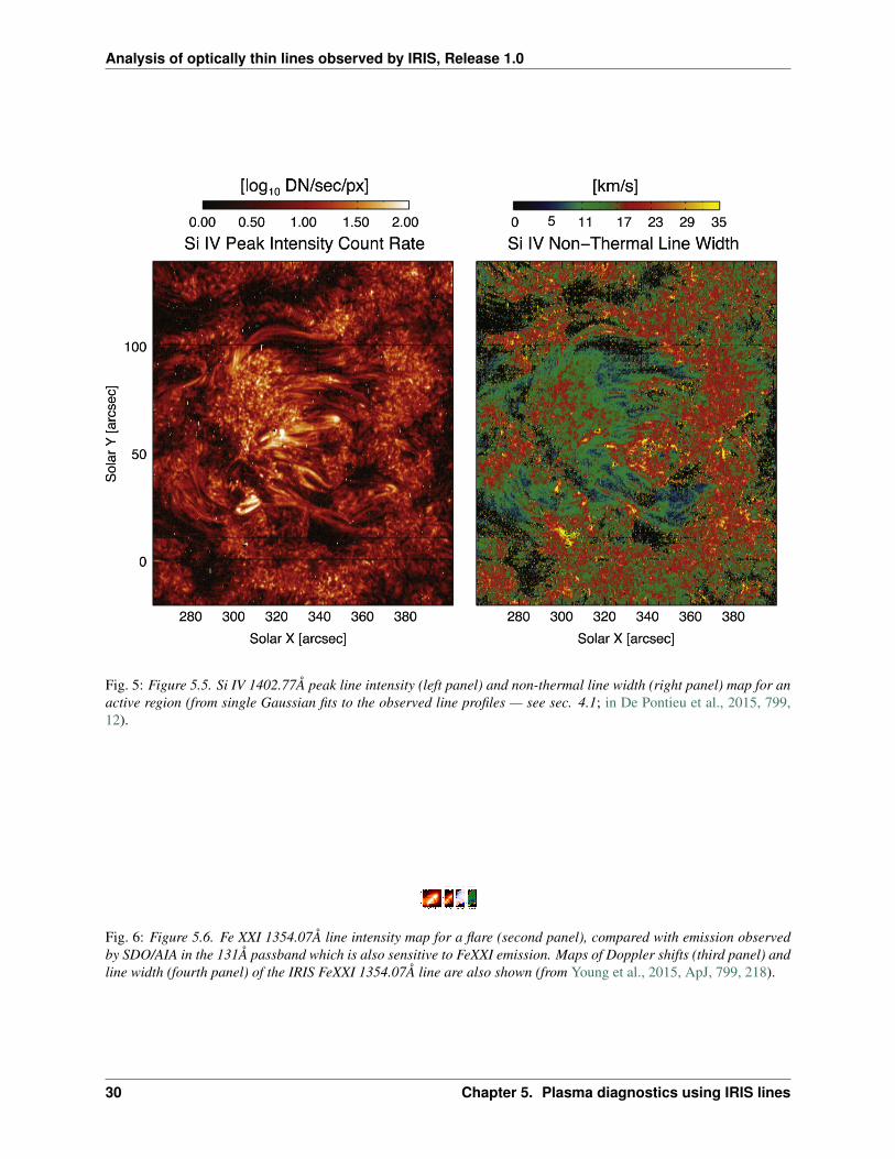
Fig. 5: Figure 5.5. Si IV 1402.77Å peak line intensity (left panel) and non-thermal line width (right panel) map for anactive region (from single Gaussian fits to the observed line profiles — see sec. 4.1; in De Pontieu et al., 2015, 799,12).

Fig. 6: Figure 5.6. Fe XXI 1354.07Å line intensity map for a flare (second panel), compared with emission observedby SDO/AIA in the 131Å passband which is also sensitive to FeXXI emission. Maps of Doppler shifts (third panel) andline width (fourth panel) of the IRIS FeXXI 1354.07Å line are also shown (from Young et al., 2015, ApJ, 799, 218).

30 Chapter 5. Plasma diagnostics using IRIS lines

Analysis of optically thin lines observed by IRIS, Release 1.0

Fig. 7: Figure 5.7. Examples of Si IV 1394Å and CII 1336Å line profiles showing asymmetries, produced by type IIspicules (from Rouppe van der Voort et al., 2015, ApJL, 799, 3).

5.2. Plasma motions: Doppler shifts and non-thermal line widths 31

Analysis of optically thin lines observed by IRIS, Release 1.0

5.3 Opacity using ratio of Si IV lines

IRIS observes two Si IV lines at 1393.75 Å and 1402.77 Å whose ratio can be used to test whether the ion is formedunder optically thin or thick conditions. In particular, a ratio close to 2 is compatible with the lines being optically thin(see e.g., Peter et al. 2014, Science, 346, 315 and Yan et al. 2015, ApJ, 811. 48). However, it is possible that the linesare optically thick and still have a ratio of about 2, so one cannot use the line ratio to conclusively state that the linesare optically thin.

While the 1402.77 Å line is largely free of blends, the 1393.75 Å line is blended with a Ni II 1393.33 Å line at around~90 km/s from at the Si IV core and with an unidentified transition, which is only visible during flares. These blendsshould be removed from the line intensity before calculating the 𝜆 1393.755/1402.770 ratio.

32 Chapter 5. Plasma diagnostics using IRIS lines